Distributed Subdata Selection for Big Data via Sampling-Based Approach

Haixiang Zhang

Center for Applied Mathematics, Tianjin University, Tianjin 300072, China

HaiYing Wang∗

Department of Statistics, University of Connecticut, Storrs, Mansfield, CT 06269, USA

Abstract

With the development of modern technologies, it is possible to gather an extraordinarily large number of

observations. Due to the storage or transmission burden, big data are usually scattered at multiple locations.

It is difficult to transfer all of data to the central server for analysis. A distributed subdata selection

method for big data linear regression model is proposed. Particularly, a two-step subsampling strategy with

optimal subsampling probabilities and optimal allocation sizes is developed. The subsample-based estimator

effectively approximates the ordinary least squares estimator from the full data. The convergence rate

and asymptotic normality of the proposed estimator are established. Simulation studies and an illustrative

example about airline data are provided to assess the performance of the proposed method.

Keywords: Allocation sizes, Big data, Distributed subsampling, Optimal subsampling, Regression

diagnostic

1. Introduction

Nowadays, big data analysis has become an interesting and important research field. The most common

feature of big data is the abundant number of observations (large n), which lays heavy burden on storage and

computation facilities. To deal with this difficulty, many efforts have been devoted in the literature. There

are mainly three directions from the view of statistical applications: divide-and-conquer, online updating,5

and subsampling. The basic idea of divide-and-conquer approach is to split the whole data into many small

data sets, and conduct statistical inference separately over each individual data set. The final estimator

can be obtained by merging estimators from all small data sets. For example, Zhao et al. (2016) considered

a partially linear framework for modeling massive heterogeneous data. Battey et al. (2018) studied the

topic on hypothesis testing and parameter estimation with a divide and conquer algorithm. Jordan et al.10

(2019) presented a communication-efficient surrogate likelihood framework for distributed statistical inference

problems. Shi et al. (2018) studied the divide and conquer method for cubic-rate estimators under massive

∗Corresponding author215 Glenbrook Rd. U-4120, Storrs, Mansfield, CT 06269, USA;Tel: 1.860.486.6142; Fax: 1.860.486.4113.Email address: haiying.wang@uconn.edu (HaiYing Wang)

Preprint submitted to Computational Statistics & Data Analysis August 28, 2020

data framework. Volgushev et al. (2019) proposed a two-step distributed method for quantile regression with

massive data sets. The online updating method focuses on big data that observations are not available all

at once. Instead, they arrive in chunks from a data stream. Schifano et al. (2016) developed some iterative15

estimating algorithms and statistical inference procedures for linear models and estimating equations with

streaming data. Wang et al. (2018a) proposed an online updating method that could incorporate new

variables for big data streams. Xue et al. (2019) proposed an online updating approach for testing the

proportional hazards assumption with big survival data.

Another popular method is the subsampling approach, where the basic idea is to select a subsample for20

the purpose of statistical inference. Ma et al. (2015) proposed an algorithmic leveraging-based sampling

procedure. Wang et al. (2018b) and Wang (2019) developed some optimal subsampling methods for logistic

regression with massive data. Wang et al. (2019) provided a novel information-based optimal subdata

selection approach. Ai et al. (2019) studied the optimal subsampling algorithms for big data generalized

linear models. Wang & Ma (2020) considered the optimal subsampling for quantile regression in big data.25

For the above-mentioned subsampling methods, one common assumption is that the data is stored in one

location. However, massive data are often partitioned across multiple servers due to the storage burden or

privacy limit. For example, Wal-mart stores generate a large number of data from different locations around

the world, and it is difficult to transmit these data to a central location; the clinical information of patients are

usually stored at different hospitals, and it is impractical to touch these data simultaneously due to personal30

privacy. To deal with this problem, we propose a distributed subdata selection method in the framework

of linear models. The main features of our approach are as follows: First, we focus on the subsampling

method for several distributed big data, where each data source has a huge number of observations. Second,

we present the optimal subsampling probabilities and allocation sizes that minimize the asymptotic mean

squared error of the resultant estimator. Third, we establish consistency and asymptotic normality of the35

proposed estimator, which are useful for statistical inference.

The remainder of this article is organized as follows: In Section 2, we propose a distributed subdata selec-

tion algorithm in the framework of sampling technique. We establish consistency and asymptotic normality

of the subsample estimator based on a general subsampling algorithm. In Section 3, we provide an optimal

sampling criterion with the focus on developing subsampling probabilities and allocation sizes, which mini-40

mize the asymptotic mean squared error of the resultant estimator. Then we develop a two-step algorithm

to approximate the optimal subsampling procedure. In Section 4, we conduct an extensive simulation study

to verify the effectiveness of our method. An application to airline data is presented in Section 5. In Section

6, we provide concluding remarks and future research topics. All proof details are given in the Appendix.

2. Distributed Subdata Selection Algorithm45

Given a covariate X ∈ Rp, we consider the linear regression model

Y = βTX + ε, (2.1)

2

where β = (β1, · · · , βp)T is a vector of regression coefficients, ε is an error term with E(ε) = 0 and V ar(ε) =

σ2. We assume that X is nonrandom, and the first component of X is 1 (β1 is the intercept). Assume that

there are K large data sources, denoted as Fn = {(Yik,Xik), i = 1, · · · , nk; k = 1, · · · ,K}, which are stored

separately at different locations. Here the sample size of the kth data source nk is much larger than the

dimension of the covariate X (nk � p), and n =∑Kk=1 nk is the total sample size.50

If we are able to analyze the full data Fn, the ordinary least squares (OLS) estimator for β is

βOLS = arg minβS(β) = arg min

β

1

2n

K∑k=1

nk∑i=1

(Yik − βTXik)2. (2.2)

It is straightforward to deduce an explicit expression of the OLS estimator with full data,

βOLS = Γ−1Ψ, (2.3)

where

Γ =1

n

K∑k=1

nk∑i=1

XikXTik, and Ψ =

1

n

K∑k=1

nk∑i=1

YikXik.

Due to storage capacity or network limitation, it is impractical to send raw data to a central server for

statistical analysis. If the estimate of β is the only thing we care about, then sending some summary

statistics from each data locations would be sufficient. However, practical data analysis seldom ends with

an estimate. For example, regression diagnostic is an integrated part of regression analysis, and it requires

to access the raw data. In addition, calculating∑nki=1 XikX

Tik still takes O(nkp

2) CPU time on each data55

location. Our aim is to select a subdata with subsample size r � n from the K data sets, where each data set

{(Yik,Xik), i = 1, · · · , nk} provides rk observations. In Algorithm 1, we present our distributed subsampling

procedure towards multiple large-scale data sets.

To establish asymptotic properties of the subsample-based estimators, we need the following regularity

conditions. Here we point out that we allow πik and rk to be dependent on the responses, hence they may60

be random.

Condition (C.1). As n→∞, Γ goes to a positive-definite matrix, where Γ is defined in (2.3).

Condition (C.2). 1n2

K∑k=1

nk∑i=1

‖Xik‖4rkπik

= OP

( K∑k=1

n2k

n2rk

)and 1

n2

K∑k=1

nk∑i=1

Y 2ik‖Xik‖2rkπik

= OP

( K∑k=1

n2k

n2rk

), where ‖ · ‖

is the Euclidean norm.

Condition (C.3). 1n3

K∑k=1

nk∑i=1

Y 3ik‖Xik‖3r2kπ

2ik

= oP (1) and 1n3

K∑k=1

nk∑i=1

‖Xik‖6r2kπ

2ik

= oP (1).65

Condition (C.1) is a common assumption in linear regression models; Conditions (C.2) and (C.3) are used

to determine the convergence rate of β, together with its asymptotic distribution. These regularity conditions

are mild and can be satisfied in many practical situations. For example, if we consider the uniform sampling

with nk = n/K, rk = r/K and πik = 1/rk, then the condition 1n2

∑Kk=1

∑nki=1

‖Xik‖4rkπik

= OP

(∑Kk=1

n2k

n2rk

)is

ensured by the moment restriction with 1n

∑Kk=1

∑nki=1 ‖Xik‖4 = O(1).70

Below we establish the convergence rate, together with the asymptotic normality of β, which play an

important role in determining the optimal subsampling probabilities πik and optimal allocation sizes rk for

i = 1, · · · , nk and k = 1, · · · ,K.

3

Algorithm 1 Distributed Subsampling Algorithm

• Sampling: Assign subsampling probabilities πik, i = 1, · · · , nk for the kth data source {(Yik,Xik), i =

1, · · · , nk} with∑nki=1 πik = 1, where k = 1, · · · ,K. Given total sampling size r, draw a random subsample

of size rk from the kth data source according to {πik; i = 1, · · · , nk}, where rk is the allocation size with∑Kk=1 rk = r. We denote the corresponding responses, covariates, and subsampling probabilities as Y ∗ik, X∗ik

and π∗ik, respectively, i = 1, · · · , rk, and k = 1, · · · ,K.

• Estimation: Minimize the following weighted least squares criterion function S∗(β) to get an estimate β

based on the subsample {(Y ∗ik,X∗ik), i = 1, · · · , rk; k = 1, · · · ,K},

S∗(β) =1

2

K∑k=1

1

nrk

{rk∑i=1

1

π∗ik(Y ∗ik − βTX∗ik)2

}. (2.4)

By solving β = arg minβS∗(β), we get a weighted least squares estimator with closed-form β = Γ∗−1Ψ∗,

where

Γ∗ =

K∑k=1

rk∑i=1

1

nrkπ∗ikX∗ik(X∗ik)T , and Ψ∗ =

K∑k=1

rk∑i=1

1

nrkπ∗ikY ∗ikX

∗ik. (2.5)

Theorem 1. If Conditions (C.1) - (C.3) hold, and suppose that n−2∑Kk=1 n

2k/rk = o(1), then with proba-

bility approaching one, for any δ > 0, there exists a finite ∆δ > 0 such that

P

||β − βOLS || ≥

{K∑k=1

n2kn2rk

}1/2

∆δ Fn

< δ. (2.6)

Moreover, conditional on Fn in probability, as r →∞ and n→∞ we have

Σ−1/2(β − βOLS)d−→ N(0, I), (2.7)

whered−→ denotes convergence in distribution,

Σ = Γ−1ΦΓ−1 = OP |Fn

(K∑k=1

n2kn2rk

)(2.8)

and

Φ =

K∑k=1

1

n2rk

nk∑i=1

(Yik − βTOLSXik)2XikXTik

πik. (2.9)

Remark 1. The condition n−2∑Kk=1 n

2k/rk = o(1) indicates that K can go to infinity, and the consistency

of β still holds in this situation. This condition is very reasonable. For example, with the uniform sampling75

where nk = n/K and rk = r/K, we know that n−2∑Kk=1 n

2k/rk = 1/r goes to zero as r →∞.

3. Optimal Subsampling Criterion

Given the subsampling size r, we need to specify the subsampling probabilities πik together with the

allocation sizes rk in Algorithm 1. An easy choice is to adopt the uniform subsampling with πik = {n−1k }nki=1

4

and rk = [r/K], for i = 1, · · · , nk and k = 1, · · · ,K, where [·] denotes the rounding operation to the80

closest integer. However, this uniform subsampling method may not be optimal, and it is more suitable to

propose a nonuniform subsampling procedure for better performance. As suggested by Wang et al. (2018b),

we can determine the optimal subsampling probabilities and optimal allocation sizes by “minimizing” the

asymptotic variance-covariance matrix Σ in (2.8). Here we adopt the idea of A-optimality from Kiefer

(1959) to define the “minimizing” of matrix Σ. Specifically, this is to minimize the trace of covariance85

matrix, tr(Σ), to derive the optimal sampling strategy. However, the calculation burden of Γ−1 is heavy.

For two positive definite matrices M1 and M2, we define the partial ordering as M1 ≥ M2 if and only if

M1 −M2 is a nonnegative definite matrix. This definition is called the Loewner-ordering. Note that the

covariance matrix Σ in (2.8) depends on πik and rk through Φ in (2.9), while Γ does not involve πik and

rk, i = 1, · · · , nk, k = 1, · · · ,K. Moreover, for two given S(1) , {(π(1)ik , r

(1)k )| i = 1, · · · , nk; k = 1, · · · ,K}90

and S(2) , {(π(2)ik , r

(2)k )| i = 1, · · · , nk; k = 1, · · · ,K}, it can be checked that Σ(S(1)) ≥ Σ(S(2)) if and only

if Φ(S(1)) ≥ Φ(S(2)). From this point of view, we only focus on minimizing tr(Φ) to specify the optimal

subsampling rule (Wang et al., 2018b). The following theorem presents the explicit expressions for optimal

subsampling probabilities and optimal allocation sizes.

Theorem 2. In Algorithm 1, the optimal subsampling probabilities (OSP) minimizing tr(Φ) are

πOSPik =|Yik − βTOLSXik|‖Xik‖∑nkj=1 |Yjk − βTOLSXjk|‖Xjk‖

, for i = 1, · · · , nk and k = 1, · · · ,K. (3.1)

For a given subsample size r, the optimal allocation sizes (OAS) rk are

rOASk = r ·∑nki=1 |Yik − βTOLSXik|‖Xik‖∑K

`=1

∑n`i=1 |Yi` − βTOLSXi`|‖Xi`‖

, for k = 1, · · · ,K. (3.2)

For practical implementation, we can use [rOASk ] as the allocation sizes for k = 1, · · · ,K, where [ · ] denotes95

the rounding operation to the closest integer. Furthermore, we need to provide βOLS for the subsampling

probabilities πOSPik and allocation sizes rOASk , where i = 1, · · · , nk and k = 1, · · · ,K. However, βOLS is

unavailable beforehand. To deal with this problem, we can use a pilot estimator β0 to replace βOLS . In

addition, for those data points with Yik being close to βTOLSXik, the corresponding subsampling probabilities

are very small. To protect the weighted criterion function S∗(β) from being inflated, we can truncate the100

|Yik − βTOLSXik| by max(|Yik − βTOLSXik|, c), where c > 0 is a specified low-bound, e.g. c = 10−6. To

summarize the above procedure, we present the implementation details in Algorithm 2.

Algorithm 2 first takes a pilot subsample of size r0 and then selects a second subsample of size r. We do

not recommend combining the two step subsamples for data analysis. The reason is that if we could conduct

statistical analysis with size r0 + r, then we could have had a better subsample by setting the second step105

sample size to r0 + r directly. Below we establish the consistency and asymptotic normality of β based on

the subsampling procedure in Algorithm 2. First we need the following regularity moment conditions:

Condition (C.4). 1n

∑Kk=1

∑nki=1 |Yik|6 = OP (1) and 1

n

∑Kk=1

∑nki=1 ‖Xik‖6 = O(1).

5

Algorithm 2 Two-Step Strategy

Step 1.

• Take a subsample size r0 by using uniform subsampling probability πik = {1/nk}nki=1 to take r0k =

[r0/K] data points from each of the K distributed units. Send the r0 data points to the central unit

and obtain a pilot estimator β0.

• Send β0 to the K distributed units to calculate uik = max(|Yik − βT0 Xik|, c)‖Xik‖, U0k =∑nki=1 uik,

and

πik(β0) =uikU0k

, for i = 1, · · · , nk and k = 1, · · · ,K. (3.3)

• Send U0k, k = 1, ...,K, to the central unit to calculate

rk(β0) =rU0k∑Kj=1 U0j

, for k = 1, · · · ,K. (3.4)

(If the distributed units can communicate, then U0k’s are shared by all units and each rk(β0) is

calculated in each distributed unit.)

• Send rk(β0)’s to the corresponding K distributed units.

Step 2.

• Draw a subsample of size rk(β0) with replacement using the subsampling probabilities πik(β0) for

i = 1, · · · , nk from the k-th unit for k = 1, · · · ,K.

• Denote the selected subsamples and associated probabilities as {(Y ∗ik,X∗ik, π∗ik), i = 1, · · · , r0k, k =

1, · · · ,K}. Send them to the central unit. Let

S∗β0

(β) =1

2

K∑k=1

1

nrk(β0)

rk(β0)∑i=1

1

π∗ik(β0)(Y ∗ik − βTX∗ik)2. (3.5)

An explicit expression of the subsample-based estimator is β = Γ∗−1(β0)Ψ∗(β0), where

Γ∗(β0) =

K∑k=1

rk(β0)∑i=1

1

nrk(β0)π∗ik(β0)X∗ik(X∗ik)T , and Ψ∗(β0) =

K∑k=1

rk(β0)∑i=1

1

nrk(β0)π∗ik(β0)Y ∗ikX

∗ik.

• Perform necessary regression diagnostics based on the selected subsample.

6

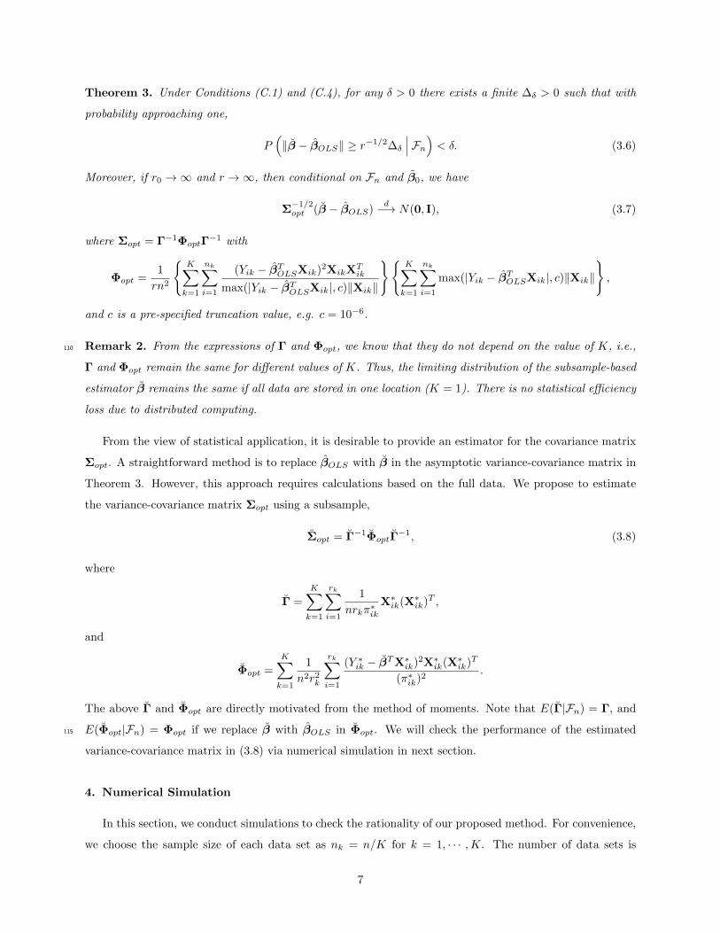
Theorem 3. Under Conditions (C.1) and (C.4), for any δ > 0 there exists a finite ∆δ > 0 such that with

probability approaching one,

P(‖β − βOLS‖ ≥ r−1/2∆δ Fn

)< δ. (3.6)

Moreover, if r0 →∞ and r →∞, then conditional on Fn and β0, we have

Σ−1/2opt (β − βOLS)

d−→ N(0, I), (3.7)

where Σopt = Γ−1ΦoptΓ−1 with

Φopt =1

rn2

{K∑k=1

nk∑i=1

(Yik − βTOLSXik)2XikXTik

max(|Yik − βTOLSXik|, c)‖Xik‖

}{K∑k=1

nk∑i=1

max(|Yik − βTOLSXik|, c)‖Xik‖

},

and c is a pre-specified truncation value, e.g. c = 10−6.

Remark 2. From the expressions of Γ and Φopt, we know that they do not depend on the value of K, i.e.,110

Γ and Φopt remain the same for different values of K. Thus, the limiting distribution of the subsample-based

estimator β remains the same if all data are stored in one location (K = 1). There is no statistical efficiency

loss due to distributed computing.

From the view of statistical application, it is desirable to provide an estimator for the covariance matrix

Σopt. A straightforward method is to replace βOLS with β in the asymptotic variance-covariance matrix in

Theorem 3. However, this approach requires calculations based on the full data. We propose to estimate

the variance-covariance matrix Σopt using a subsample,

Σopt = Γ−1ΦoptΓ−1, (3.8)

where

Γ =K∑k=1

rk∑i=1

1

nrkπ∗ikX∗ik(X∗ik)T ,

and

Φopt =

K∑k=1

1

n2r2k

rk∑i=1

(Y ∗ik − βTX∗ik)2X∗ik(X∗ik)T

(π∗ik)2.

The above Γ and Φopt are directly motivated from the method of moments. Note that E(Γ|Fn) = Γ, and

E(Φopt|Fn) = Φopt if we replace β with βOLS in Φopt. We will check the performance of the estimated115

variance-covariance matrix in (3.8) via numerical simulation in next section.

4. Numerical Simulation

In this section, we conduct simulations to check the rationality of our proposed method. For convenience,

we choose the sample size of each data set as nk = n/K for k = 1, · · · ,K. The number of data sets is

7

K = 2 and 100, respectively. The vector of regression coefficients is β = (0.5, · · · , 0.5)′ with p = 5 and 50,120

respectively. Denote X = (1, X′)′ with X = (X2, · · · , Xp)′. Let ΣX = (0.5|i−j|) be a covariance matrix with

1 ≤ i, j ≤ p− 1. We consider the following three cases for the generation of covariate X:

Case I: The X has a multivariate normal distribution, that is, X ∼ N(0,ΣX).

Case II: The X has a multivariate lognormal distribution, that is, X ∼ LN(0,ΣX).

Case III: The X has a multivariate t distribution with degrees of freedom v = 2, that is, X ∼ t2(0,ΣX).125

We generate the error term ε from N(0, 1). The r0 in Step 1 of Algorithm 2 is chosen as r0 = 500, and the

subsample size r = 500, 800 and 1000, respectively. All the simulation results in Tables 1 and 2, together

with Figures 4.2 and 4.3 are based on 1000 replications with total sample size n = 106.

In Tables 1 and 2, we present the results of β1, which include the estimated biases (BIAS) given by

the sample mean of the estimates minus the OLS estimator in (2.2), the sampling standard error (SE) of130

the estimates, the sample mean of the estimated standard errors (ESE), and the empirical 95% coverage

probabilities (CP) based on normal approximation. From the results in Tables 1 and 2, we can see that

the subsample-based estimators are unbiased, the estimated and empirical standard errors are similar, and

the coverage probabilities of the 95% confidence intervals are satisfactory. Furthermore, the performances

of subsample-based estimators become better as r increases. Results for other components of β are similar135

and thus are omitted.

Table 1: Simulation results on the two-step subsample estimator β1 with K = 2†.

p = 5 p = 50

r BIAS SE ESE CP BIAS SE ESE CP

Case I 500 −0.0021 0.0385 0.0389 0.958 −0.0067 0.0470 0.0435 0.927

800 −0.0008 0.0298 0.0305 0.960 −0.0053 0.0349 0.0335 0.933

1000 −0.0014 0.0281 0.0276 0.949 0.0002 0.0299 0.0297 0.945

Case II 500 0.0051 0.0740 0.0742 0.952 0.0115 0.1789 0.1728 0.942

800 −0.0022 0.0576 0.0584 0.955 0.0007 0.1382 0.1304 0.931

1000 0.0016 0.0522 0.0520 0.954 0.0016 0.1219 0.1172 0.940

Case III 500 −0.0024 0.0470 0.0469 0.948 0.0043 0.0696 0.0674 0.939

800 −0.0011 0.0381 0.0377 0.949 −0.0027 0.0581 0.0556 0.941

1000 −0.0002 0.0380 0.0373 0.945 −0.0006 0.0490 0.0477 0.947

†“BIAS” denotes the biases of subsample estimates; “ SE” denotes the sampling standard error of the estimates; “ESE” denotes

the sample mean of the estimated standard errors; “CP” denotes the empirical 95% coverage probabilities.

8

Table 2: Simulation results on the two-step subsample estimator β1 with K = 100†.

p = 5 p = 50

r BIAS SE ESE CP BIAS SE ESE CP

Case I 500 −0.0021 0.0397 0.0388 0.941 −0.0036 0.0470 0.0434 0.928

800 0.0005 0.0305 0.0306 0.956 −0.0046 0.0357 0.0337 0.932

1000 0.0006 0.0269 0.0272 0.954 0.0014 0.0317 0.0301 0.931

Case II 500 0.0002 0.0720 0.0745 0.966 0.0212 0.1826 0.1706 0.938

800 0.0025 0.0564 0.0583 0.956 −0.0207 0.1395 0.1319 0.925

1000 −0.0002 0.0537 0.0528 0.943 0.0068 0.1199 0.1169 0.942

Case III 500 −0.0030 0.0525 0.0501 0.942 0.0032 0.0870 0.0829 0.939

800 0.0014 0.0390 0.0376 0.939 0.0006 0.0590 0.0566 0.940

1000 −0.0026 0.0344 0.0337 0.942 0.0062 0.0574 0.0560 0.948

†“BIAS” denotes the biases of subsample estimates; “ SE” denotes the sampling standard error of the estimates; “ESE” denotes

the sample mean of the estimated standard errors; “CP” denotes the empirical 95% coverage probabilities.

In addition to parameter estimates, we also consider the usefulness of a subsample in regression diag-

nostics. Figure 4.1 is a residual plot with residuals vs. fitted values for Case I, where K = 2, p = 5 and

r = 1000. The residual plot from the subsample has a similar pattern with that from full data, which reveals

potential usefulness of the OSC-based subsample in regression diagnostics.140

(a) Fitted values vs. residuals with subsample. (b) Fitted values vs. residuals with full data.

Figure 4.1: Residual plots with K = 2, p = 5 and r = 1000 (Case I).

9

400 600 800 1000 1200

0.02

0.03

0.04

0.05

0.06

r

AS

E

OSC UNIF LEV

(a) Case I with K = 2, p = 5.

400 600 800 1000 1200

0.03

0.04

0.05

0.06

0.07

r

AS

E

OSC UNIF LEV

(b) Case I with K = 100, p = 50.

400 600 800 1000 1200

0.01

50.

020

0.02

50.

030

0.03

50.

040

r

AS

E

OSC UNIF LEV

(c) Case II with K = 2, p = 5.

400 600 800 1000 1200

0.01

00.

020

0.03

00.

040

r

AS

E OSC UNIF LEV

(d) Case II with K = 100, p = 50.

400 600 800 1000 1200

0.00

00.

010

0.02

00.

030

r

AS

E

OSC UNIF LEV

(e) Case III with K = 2, p = 5.

400 600 800 1000 1200

0.00

0.01

0.02

0.03

0.04

r

AS

E

OSC UNIF LEV

(f) Case III with K = 100, p = 50.

Figure 4.2: The ASEs for different subsampling methods.

10

400 600 800 1000 1200

0.02

0.06

0.10

0.14

r

AS

E

UNIF LEV

(a) Intercept with K = 2, p = 5.

400 600 800 1000 1200

0.00

50.

010

0.01

50.

020

0.02

50.

030

r

AS

E

UNIF LEV

(b) Slope with K = 2, p = 5.

400 600 800 1000 12000.00

0.05

0.10

0.15

0.20

0.25

0.30

r

AS

E

UNIF LEV

(c) Intercept with K = 100, p = 50.

400 600 800 1000 1200

0.01

00.

015

0.02

00.

025

0.03

0

r

AS

E UNIF LEV

(d) Slope with K = 100, p = 50.

Figure 4.3: ASEs of UNIF and LEV for estimating the intercept and slope parameters with Case II.

To investigate the superiority of our optimal subsampling criterion (OSC), we compare the OSC with

uniform subsampling (UNIF), whose subsampling probabilities πik = 1/nk and allocation sizes rk = [r/K],

for i = 1, · · · , nk and k = 1, · · · ,K. Moreover, we also consider the leverage-based subsampling (LEV;

Ma, et al., 2015). To ensoure the best performance of the LEV method in parameter estimation, exact full

data statistical leverage scores are used to derive the subsampling probabilities, i.e., πik = hik/∑nkj=1 hjk for145

i = 1, ..., nk, where hik = XTik(XT

fullXfull)−1Xik and Xfull is the full data design matrix. The allocation

sizes are taken as rk = [r/K], k = 1, · · · ,K. Let SElj denote the estimated standard error for βj in the

lth repetition of the simulation, and define SEl = 1p

∑pj=1 SElj . Here we calculate the average of SEl

based on 1000 repetition of the simulation i.e., ASE =∑1000l=1 SEl/1000. For p = 5 and 50, the results are

11

presented in Figure 4.2. It is seen that the ASEs of OSC are much smaller than those of the UNIF and150

LEV methods. The performances of LEV are better than UNIF in Cases I and III, while the LEV has a

much larger ASE than UNIF in Case II. In Case II the covariate distribution is skewed, and we see that the

UNIF out performs the LEV. To better understand this unexpected performance of the LEV method with

asymmetrically distributed covariates, we calculated ASE’s of the intercept and slope estimators separately.

Figure 4.3 shows the results for the LEV and UNIF methods in Case II. We see that the LEV has a much155

larger ASE than the UNIF towards the estimation of the intercept, which leads to the corresponding results

in Case II of Figure 4.2.

We also use simulation to evaluate the computation efficiency of our method. First we generate data

using the same mechanism as the above situation with Case I. All computations are carried out on a laptop

running R software with 16GB random-access memory (RAM). Given a pilot subsample size r0, we select160

r0k = [r0/K] data points from each of the K data units and send them back to the central place to obtain

a pilot estimator β0. The pilot β0 is then send to all data units to calculate U0k and πik(β0) as in (3.3).

Only the K scalars U0k’s need to be send to the central unit to calculate scalars rk(β0)’s as in (3.4), which

are then send to distributed units as subsample sizes. From each data unit, rk(β0) data points are selected

and they are sent to the central unit along with their associate πik(β0)’s for final data analysis. In Table 3,165

we report the required CPU times (in seconds) to obtain β with K = 2, r0 = 1000, p = 5, 50, 300 and 500,

where Algorithm 2 is implemented on a single core. Of note, these times are CPU times for implementing

each method in the RAM, while the times to generate data are not counted. Moreover, these times are the

mean CPU times of 10 repetitions. For the LEV method, the leverage scores are approximated using the

fast algorithm in Drineas et al. (2012). The computing times for the UNIF and the full data methods are170

also reported for comparison. For the full data method, Γk’s and Ψk’s for k = 1, · · · ,K, are calculated

from each data block, and then the estimator is calculated as βOLS = (∑Kk=1 Γk)−1

∑Kk=1 Ψk. That is to

say the CPU times for full data method mainly consist of the calculation of the summary statistics, and

the communication cost is negligible. It is seen from the results that the UNIF is much faster than the

other methods. The reason is that there is no need for UNIF to calculate subsampling probabilities and175

allocation sizes, so it requires less RAM and CPU times as well. Our proposed OSC method has significant

computational advantages over the LEV and full data methods. In Table 4, we show the comparisons of

ASEs for OSC and UNIF methods when the computation times are similar in Case III, where K = 2 and

r0 = 1000. The results indicate that the OSC and UNIF may have similar estimation efficiency with similar

CPU times. However, since UNIF uses larger sample sizes, it requires larger memory. Hence, our proposed180

method achieves the same estimation efficiency with less computing resources.

12

Table 3: The CPU times of subsampling methods with r = 1000 (seconds)†.

Method n = 3× 105 n = 5× 105 106

p=5 OSC 0.043 0.068 0.129

UNIF 0.008 0.016 0.033

LEV 0.739 1.288 3.462

Full data 0.061 0.111 0.255

p=50 OSC 0.180 0.325 0.610

UNIF 0.016 0.018 0.022

LEV 1.452 2.469 4.963

Full data 1.200 2.134 3.809

p=300 OSC 0.965 1.403 5.293

UNIF 0.061 0.062 0.161

LEV 3.906 6.593 21.865

Full data 21.037 32.589 85.873

p=500 OSC 1.827 2.359 5.934

UNIF 0.180 0.181 0.203

LEV 6.562 10.636 32.853

Full data 53.996 85.730 178.572

† “OSC” denotes our optimal subsampling criterion;“UNIF” denotes uniform sampling;

“LEV” denotes leverage-based subsampling.

Table 4: Comparisons of CPU times between OSC and UNIF with Case III (in seconds)†.

n = 3× 105 n = 5× 105

CPU r ASE CPU r ASE

p = 5 OSC 0.034 17500 0.00246 0.069 27500 0.00192

UNIF 0.033 45000 0.00234 0.059 75000 0.00172

p = 50 OSC 0.204 17500 0.00209 0.278 15000 0.00214

UNIF 0.211 35000 0.00241 0.236 35000 0.00236

p = 300 OSC 1.348 5500 0.00695 1.762 7500 0.00552

UNIF 1.210 7500 0.00680 1.580 9700 0.00579

p = 500 OSC 3.922 6000 0.00784 5.186 7000 0.00663

UNIF 4.086 7500 0.00736 4.747 9000 0.00651

† “OSC” denotes the optimal subsampling criterion;“UNIF” denotes uniform sampling;

“CPU” denotes computation time.

13

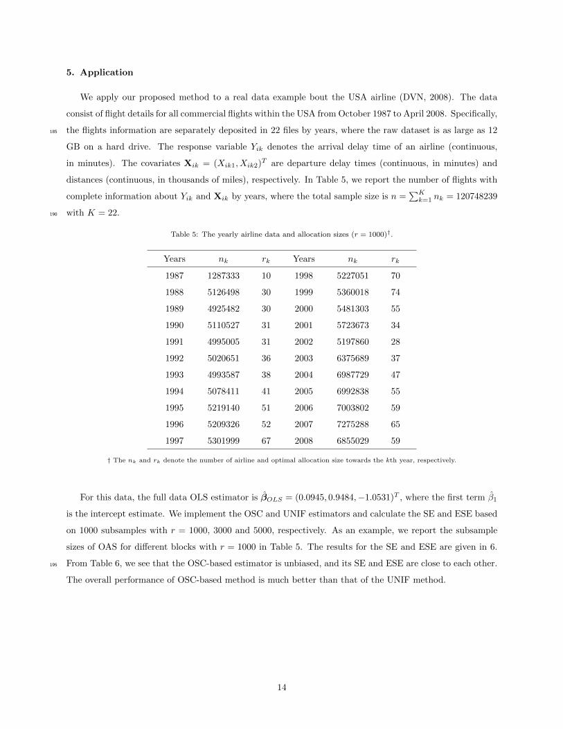
5. Application

We apply our proposed method to a real data example bout the USA airline (DVN, 2008). The data

consist of flight details for all commercial flights within the USA from October 1987 to April 2008. Specifically,

the flights information are separately deposited in 22 files by years, where the raw dataset is as large as 12185

GB on a hard drive. The response variable Yik denotes the arrival delay time of an airline (continuous,

in minutes). The covariates Xik = (Xik1, Xik2)T are departure delay times (continuous, in minutes) and

distances (continuous, in thousands of miles), respectively. In Table 5, we report the number of flights with

complete information about Yik and Xik by years, where the total sample size is n =∑Kk=1 nk = 120748239

with K = 22.190

Table 5: The yearly airline data and allocation sizes (r = 1000)†.

Years nk rk Years nk rk

1987 1287333 10 1998 5227051 70

1988 5126498 30 1999 5360018 74

1989 4925482 30 2000 5481303 55

1990 5110527 31 2001 5723673 34

1991 4995005 31 2002 5197860 28

1992 5020651 36 2003 6375689 37

1993 4993587 38 2004 6987729 47

1994 5078411 41 2005 6992838 55

1995 5219140 51 2006 7003802 59

1996 5209326 52 2007 7275288 65

1997 5301999 67 2008 6855029 59

† The nk and rk denote the number of airline and optimal allocation size towards the kth year, respectively.

For this data, the full data OLS estimator is βOLS = (0.0945, 0.9484,−1.0531)T , where the first term β1

is the intercept estimate. We implement the OSC and UNIF estimators and calculate the SE and ESE based

on 1000 subsamples with r = 1000, 3000 and 5000, respectively. As an example, we report the subsample

sizes of OAS for different blocks with r = 1000 in Table 5. The results for the SE and ESE are given in 6.

From Table 6, we see that the OSC-based estimator is unbiased, and its SE and ESE are close to each other.195

The overall performance of OSC-based method is much better than that of the UNIF method.

14

Table 6: Subsample estimator and (SE, ESE) for the airline data†.

β OSC UNIF

r = 1000 β1 0.1166 (1.2541, 1.2489) −0.1714 (1.1272, 0.7129)

β2 0.9479 (0.0108, 0.0108) 0.9940 (0.1377, 0.0294)

β3 −0.9984 (1.3725, 1.3897) −1.1700 (1.0399, 0.9530)

r = 3000 β1 0.1333 (0.7568, 0.7355) −0.1310 (0.9320, 0.4988)

β2 0.9478 (0.0067, 0.0069) 0.9829 (0.1309, 0.0338)

β3 −1.0759 (0.8108, 0.7927) −1.1082 (0.6425, 0.5673)

r = 5000 β1 0.0876 (0.5606, 0.5451) −0.0413 (0.8769, 0.4732)

β2 0.9482 (0.0050, 0.0051) 0.9709 (0.1259, 0.0409)

β3 −1.0527 (0.6043, 0.5973) −1.0978 (0.4867, 0.4478)

† β1 is an intercept; “OSC” denotes optimal subsampling criterion;“UNIF” denotes uniform subsampling.

Finally, we use a subsample to create a residual plot to check the appropriateness of using a linear

regression model on the data. For comparison, we also use a server with 128G RAM to create the same plot

from the full data. We present the results in Figure 5.1, where OSC-based subsample size r= 5000. It is seen

that there is some potential cluster pattern in the data, and the subsample residual plot also identifies this.200

This indicates that a more complicated model, such as a mixture model, may improve the goodness-of-fit.

However, this is beyond the scope of the current paper and we will investigate it in a future project. In fact,

the R square statistic for the whole data is R2 = 0.7607 (calculated on the server), which is not very small,

indicating that a linear regression is still a useful model for the data. The clustering patter for the data is

more evident if we plot the fitted values against the observed responses as shown in Figure 5.2.205

15

(a) Residual plot from a subsample of r = 5000. (b) Residual plot from the full data.

Figure 5.1: Residual plots from an OSC-based subsample (r= 5000) and from the full data.

(a) Fitted values vs. observed responses in a subsam-

ple of r = 5000.

(b) Fitted values vs. observed responses in the full

data.

Figure 5.2: Fitted values vs. observed responses in an OSC-based subsample (r= 5000) and in the full data.

6. Concluding Remarks

In this paper, we have proposed an optimal subsampling method for distributed and massive data in the

context of linear models. The convergence rate and asymptotic normality of the subsample-based estimators

were established. The optimal subsampling probabilities and optimal allocation sizes were provided. We have

16

also used numerical results to show that the OSC-based subsample selection procedure was more efficient210

than the UNIF-based method in parameter estimation. Simulations and a real data example have revealed

the effectiveness of our method.

There are several topics to investigate in the future. First, we have illustrated the usefulness of OSC-

based subsample in regression diagnostics by numerical studies. However, it is difficult to theoretically

validate that the OSC-based subsample is optimal towards regression diagnostics. The optimal subsample215

selection for regression diagnostics with big data needs further research. Second, it is interesting to extend

our distributed subsampling method to other models, such as the logistic regression of Wang et al. (2018b)

and the generalized linear models in Ai et al. (2019). Third, a larger πi indicates that the data point

(Xi, Yi) contains more information about β, but it has a smaller weight in the object function (2.4). To

improve contributions of those more informative points for parameter estimation, it is desirable to propose220

an un-weighted estimator as Wang (2019) in the framework of distributed subsampling.

Acknowledgements

The authors would like to thank the Editor, the Associate Editor and the reviewer for their constructive

and insightful comments that greatly improved the manuscript. The corresponding author’s work was

supported by NSF grant DMS-1812013.225

17

7. Appendix

Below, we give the proofs for Theorems 1 − 3. Note that from Cauchy-Schwarz inequality Condition

(C.2) implies that 1n2

K∑k=1

nk∑i=1

Yik‖Xik‖3rkπik

= OP

( K∑k=1

n2k

n2rk

), and from Holder’s inequality, Condition (C.3)

implies that 1n3

K∑k=1

nk∑i=1

Y 2ik‖Xik‖4r2kπ

2ik

= oP (1) and 1n3

K∑k=1

nk∑i=1

Yik‖Xik‖5r2kπ

2ik

= oP (1). We first establish the following

lemma.230

Lemma 1. If Conditions (C.1) and (C.2) hold, then conditionally on Fn we have

Γ∗ − Γ = OP |Fn

{ K∑k=1

n2kn2rk

}1/2 , (A.1)

Ψ∗ −Ψ = OP |Fn

{ K∑k=1

n2kn2rk

}1/2 , (A.2)

and

∂S∗(βOLS)

∂β= OP |Fn

{ K∑k=1

n2kn2rk

}1/2 . (A.3)

Proof. It is straightforward to deduce that E(Γ∗|Fn) = Γ holds. Moreover, for any component Γ∗j1j2 of Γ∗

with 1 ≤ j1 ≤ j2 ≤ p, we have

V ar(Γ∗j1j2 |Fn) =

K∑k=1

n2kn2rk

{1

n2k

nk∑i=1

1

πik(Xikj1Xikj2)

2 −( 1

nk

nk∑i=1

Xikj1Xikj2

)2}

≤K∑k=1

n2kn2rk

{1

n2k

nk∑i=1

‖Xik‖4

πik

}

= OP |Fn

(K∑k=1

n2kn2rk

), (A.4)

where the equality (A.4) holds by Condition (C.2). Then Markov’s inequality leads to (A.1). Similarly, we

know E(Ψ∗|Fn) = Ψ. Besides, for any component Ψ∗j of Ψ∗ with 1 ≤ j ≤ p,

V ar(Ψ∗j |Fn) = E(Ψ∗j −Ψj |Fn)2

=

K∑k=1

n2kn2rk

1

n2k

nk∑i=1

1

πikY 2ikX

2ikj −

(1

nk

nk∑i=1

YikXikj

)2

≤K∑k=1

n2kn2rk

{1

n2k

nk∑i=1

1

πikY 2ik‖Xik‖2

}

= OP |Fn

(K∑k=1

n2kn2rk

),

where the last equality is due to Condition (C.2). Thus, (A.2) holds using the Markov’s inequality.

18

Finally, direct calculation yields that

E

(∂S∗(βOLS)

∂βFn

)=∂S(βOLS)

∂β= 0. (A.5)

By Condition (C.2), for j = 1, · · · , p, we can derive that

V ar

(∂S∗(βOLS)

∂βjFn

)=

K∑k=1

n2kn2rk

{ nk∑i=1

(Yik − βTOLSXik)2X2ikj

n2kπik−[ 1

nk

nk∑i=1

(Yik − βTOLSXik)Xikj

]2}≤

K∑k=1

n2kn2rk

nk∑i=1

Y 2ik‖Xik‖2 − 2Yik‖Xik‖3‖βOLS‖+ ‖βOLS‖2‖Xik‖4

n2kπik

= OP |Fn

(K∑k=1

n2kn2rk

). (A.6)

Using (A.5), (A.6) and Markov’s inequality, (A.3) holds. This ends the proof. �

Proof of Theorem 1. Note that

∂S∗(βOLS)

∂β= −

K∑k=1

1

rk

{rk∑i=1

(Y ∗ik − βTOLSX∗ik)X∗iknπ∗ik

}

= −(Ψ∗ − Γ∗Γ−1Ψ). (A.7)

From (A.1) in Lemma 1,

Γ∗−1 − Γ−1 = Γ∗−1(Γ− Γ∗)Γ−1 = OP |Fn

{ K∑k=1

n2kn2rk

}1/2 . (A.8)

After some direct calculation, by (A.3), (A.7) and (A.8) we can deduce the expression

β − βOLS = Γ∗−1Ψ∗ − Γ−1Ψ

= −Γ∗−1∂S∗(βOLS)

∂β

= −Γ−1∂S∗(βOLS)

∂β+ (Γ−1 − Γ∗−1)

∂S∗(βOLS)

∂β

= −Γ−1∂S∗(βOLS)

∂β+OP |Fn

(K∑k=1

n2kn2rk

)(A.9)

= OP |Fn

{ K∑k=1

n2kn2rk

}1/2 .

Thus, the convergence rate of β in (2.6) is established. In what follows, we need to establish the asymptotic

distribution of ∂S∗(βOLS)∂β . Since

∂S∗(βOLS)

∂β= −

K∑k=1

1

rk

{rk∑i=1

(Y ∗ik − βTOLSX∗ik)X∗iknπ∗ik

}

19

= −K∑k=1

rk∑i=1

ζ∗ik,

where ζ∗ik =(Y ∗ik−β

TOLSX

∗ik)X

∗ik

nrkπ∗ik, i = 1, · · · , rk, and k = 1, · · · ,K. Given Fn, the ζ∗ik are independent, and for

every η > 0,

K∑k=1

rk∑i=1

E{‖ζ∗ik‖2I(‖ζ∗ik‖ > η) Fn

}≤

K∑k=1

rk∑i=1

1

ηE{‖ζ∗ik‖3I(‖ζ∗ik‖ > η) Fn

}≤

K∑k=1

rk∑i=1

1

ηE{‖ζ∗ik‖3 Fn

}=

K∑k=1

1

r2kηn3

nk∑i=1

(Yik − βTOLSXik)3‖Xik‖3

π2ik

≤K∑k=1

1

n3r2k

{1

η

nk∑i=1

Y 3ik‖Xik‖3 − 3Y 2

ik‖βOLS‖‖Xik‖4 + 3Yik‖βOLS‖2‖Xik‖5 − ‖βOLS‖3‖Xik‖6

π2ik

}

= oP |Fn(1),

where the last equation is from Condition (C.3). Moreover, we have that

K∑k=1

rk∑i=1

Cov(ζ∗ik|Fn) =

K∑k=1

n2kn2rk

{ nk∑i=1

(Yik − βTOLSXik)2XikXTik

n2kπik

−[ 1

nk

nk∑i=1

(Yik − βTOLSXik)Xik

][ 1

nk

nk∑i=1

(Yik − βTOLSXik)XTik

]}= Φ−∆1, (A.10)

where

∆1 =1

n2

K∑k=1

1

rk

[ nk∑i=1

(Yik − βTOLSXik)Xik

][ nk∑i=1

(Yik − βTOLSXik)XTik

]. (A.11)

For convenience, we denote Xk and Yk as the design matrix and responses of kth data sets, k = 1, · · · ,K.

Similarly, let Xfull and Yfull be the design matrix and responses of full data. It is straightforward to

deduce that

E

[nk∑i=1

(Yik − βTOLSXik)Xik

]= E(XT

kYk −XTkXkβOLS) = 0.

Hence,

E

{[nk∑i=1

(Yik − βTOLSXik)Xik

][nk∑i=1

(Yik − βTOLSXik)XTik

]}= Cov(XT

kYk −XTkXkβOLS). (A.12)

Notice that

XTkYk −XT

kXkβOLS = XTkYk −XT

kXk(XTfullXfull)

−1K∑`=1

XT` Y`

20

= XTkYk −XT

kXk(XTfullXfull)

−1XTkYk︸ ︷︷ ︸

R1

−XTkXk(XT

fullXfull)−1

K∑` 6=k

XT` Y`︸ ︷︷ ︸

R2

.

In view of the following expressions,

Cov(R1) = σ2XTk {I− 2Xk(XT

fullXfull)−1XT

k + Xk(XTfullXfull)

−1XTkXk(XT

fullXfull)−1XT

k }Xk,

and

Cov(R2) = σ2XTkXk(XT

fullXfull)−1

K∑6=k

XT` X`(X

TfullXfull)

−1XTkXk,

we have

Cov(XTkYk −XT

kXkβOLS) = σ2{XTkXk −XT

kXk(XTfullXfull)

−1XTkXk} (A.13)

= σ2

{nk∑i=1

XikXTik −

nk∑i=1

XikXTik(XT

fullXfull)−1XikX

Tik

}.

Noting that XTfullXfull is positive-definite for large n and thus

∥∥XikXTik(XT

fullXfull)−1XikX

Tik

∥∥ ≤ ∥∥XikXTik

∥∥ , (A.14)

we know that ∥∥∥Cov(XTkYk −XT

kXkβOLS)∥∥∥ ≤ 2σ2

nk∑i=1

‖Xik‖2. (A.15)

Thus, from (A.11), (A.12) and (A.15),

E(∆1) ≤ 2σ2

n2

K∑k=1

nk∑i=1

‖Xik‖2

rk≤ 2σ2

n2

K∑k=1

nk∑i=1

‖Xik‖4

rk= o(1), (A.16)

where the last step is from Condition (C.2). Since ∆1 is positive semidefinite, we know that ∆1 = op(1),

and therefore (A.10) implies that

K∑k=1

rk∑i=1

Cov(ζ∗ik) = Φ + oP (1).

From the Lindeberg-Feller central limit theorem in Proposition 2.27 of van der Vaart (1998) and Slutsky’s

theorem, conditionally on Fn,

Φ−1/2∂S∗(βOLS)

∂β

d−→ N(0, I). (A.17)

By Conditions (C.2) and (C.3), it can be proved that

Σ = Γ−1ΦΓ−1 = OP |Fn

(K∑k=1

n2kn2rk

).

21

Therefore, (A.9), (A.17) and the Slutsky’s theorem lead to the asymptotic distribution in (2.7). This ends

the proof. �

Proof of Theorem 2. From (2.8) and (2.9), it can be calculated that

tr(Φ) =

K∑k=1

1

rkn2

nk∑i=1

[1

πik(Yik − βTOLSXik)2‖Xik‖2

]

=

K∑k=1

1

rkn2·

(nk∑i=1

πik

)·nk∑i=1

[1

πik(Yik − βTOLSXik)2‖Xik‖2

]

≥K∑k=1

1

rkn2

[nk∑i=1

|Yik − βTOLSXik|‖Xik‖

]2(A.18)

=

(K∑k=1

rkr

)·K∑k=1

1

rkn2

[nk∑i=1

|Yik − βTOLSXik|‖Xik‖

]2

≥

{K∑k=1

1

nr1/2

nk∑i=1

|Yik − βTOLSXik|‖Xik‖

}2

,

where the inequality (A.18) is from the Cauchy-Schwarz inequality and the equality of it holds if and only235

if when πik are proportional to |Yik − βTOLSXik|‖Xik‖, namely πik = C1|Yik − βTOLSXik|‖Xik‖ for some

constant C1 > 0. Similarly, the last equality holds if and only if when rk = C2

∑nki=1 |Yik − βTOLSXik|‖Xik‖

for some C2 > 0. This completes the proof. �

Proof of Theorem 3. First, we need to prove the following two conclusions

Γ∗(β0)− Γ = OP |Fn(r−1/2), (A.19)

∂S∗β0

(βOLS)

∂β= OP |Fn(r−1/2), (A.20)

where Γ∗(β0) =∑Kk=1

∑rk(β0)i=1

1nrk(β0)π∗ik(β0)

X∗ik(X∗ik)T . By direct calculation,

E(Γ∗(β0)|Fn) = Eβ0{E(Γ∗(β0)|Fn, β0)} = Eβ0

(Γ|Fn) = Γ. (A.21)

Here Eβ0denotes the expectation with respect to the distribution of β0 given Fn. For any component

Γ∗j1j2(β0) of Γ∗(β0) with 1 ≤ j1 ≤ j2 ≤ p,

V ar(Γ∗j1j2(β0)|Fn, β0) =

K∑k=1

1

rk(β0)

1

n2

nk∑i=1

1

πik(β0)(Xikj1Xikj2)2 −

(nk∑i=1

1

nXikj1Xikj2

)2

≤K∑k=1

1

rk(β0)

{1

n2

nk∑i=1

1

πik(β0)‖Xik‖4

}

≤ 1

r

(1

n

K∑k=1

nk∑i=1

‖Xik‖3

c

){1

n

K∑k=1

nk∑i=1

(|Yik − βT0 Xik|+ c)‖Xik‖

}

= OP (r−1), (A.22)

22

where the equality (A.22) is from Condition (C.4). Thus,

V ar(Γ∗j1j2(β0)|Fn) = Eβ0{V ar(Γ∗j1j2(β0)|Fn, β0)} = OP |Fn(r−1). (A.23)

From (A.21) and (A.23) together with Markov’s inequality, (A.19) follows. Note that

∂S∗β0

(βOLS)

∂β= −

K∑k=1

1

rk(β0)·

rk(β0)∑i=1

(Y ∗ik − βTOLSX∗ik)X∗iknπ∗ik(β0)

= −[Ψ∗(β0)− Γ∗(β0)Γ−1Ψ].

Similar to (A.21) and (A.23), by Condition (C.4) we can get that

E

∂S∗β0

(βOLS)

∂βFn

= 0, and V ar

∂S∗β0

(βOLS)

∂βFn

= OP |Fn(r−1). (A.24)

Then, (A.20) holds from (A.24) and Markov’s inequality.

Next, we begin to prove the convergence rate of β. From (A.19),

Γ−1 − Γ∗−1(β0) = Γ∗−1(β0){Γ∗(β0)− Γ}Γ−1

= OP |Fn(r−1/2). (A.25)

By careful calculation, we can derive that

β − βOLS = Γ∗−1(β0)Ψ∗(β0)− Γ−1Ψ

= −Γ∗−1(β0)∂S∗

β0(βOLS)

∂β

= −Γ−1∂S∗

β0(βOLS)

∂β+ {Γ−1 − Γ∗−1(β0)}

∂S∗β0

(βOLS)

∂β

= −Γ−1∂S∗

β0(βOLS)

∂β+OP |Fn

(r−1)

(A.26)

= OP |Fn

(r−1/2

).

Lastly, we start to establish the asymptotic distribution of β. Note that

∂S∗β0

(βOLS)

∂β= −

K∑k=1

1

rk(β0)·

rk(β0)∑i=1

(Y ∗ik − βTOLSX∗ik)X∗iknπ∗ik(β0)

= −

K∑k=1

rk(β0)∑i=1

ζ∗ik(β0),

where ζ∗ik(β0) = 1rk(β0)

·{

(Y ∗ik−βTOLSX

∗ik)X

∗ik

nπ∗ik(β0)

}, for i = 1, · · · , nk, and k = 1, · · · ,K. Given Fn and β0, the

ζik(β0) are independent. For every η > 0,

K∑k=1

rk(β0)∑i=1

E{‖ζ∗ik(β0)‖2I(‖ζ∗ik(β0)‖ > η) Fn, β0

}

23

≤K∑k=1

rk(β0)∑i=1

1

ηE{‖ζ∗ik(β0)‖3I(‖ζ∗ik(β0)‖ > η) Fn, β0

}

≤K∑k=1

rk(β0)∑i=1

1

ηE{‖ζ∗ik(β0)‖3 Fn, β0

}≤

K∑k=1

1

r2k(β0)η

nk∑i=1

|Yik − βTOLSXik|3‖Xik‖3

n3π2ik(β0)

=1

ηr2

K∑k=1

nk∑i=1

1

n

|Yik − βTOLSXik|3‖Xik‖max(|Yik − βT0 Xik|2, c2)

·

(1

n

K∑k=1

nk∑i=1

max(|Yik − βT0 Xik|, c)‖Xik‖

)2

≤ 1

ηr2

{1

n

K∑k=1

nk∑i=1

|Yik − βTOLSXik|3‖Xik‖c2

}·

(1

n

K∑k=1

nk∑i=1

(|Yik − βT0 Xik|+ c)‖Xik‖

)2

= OP (r−2),

where the last equality is from Condition (C.4). Moreover, we can prove that

K∑k=1

rk∑i=1

Cov{ζ∗ik(β0)|Fn, β0} =

K∑k=1

n2kn2rk(β0)

{ nk∑i=1

(Yik − βTOLSXik)2XikXTik

n2kπik(β0)

−[ 1

nk

nk∑i=1

(Yik − βTOLSXik)Xik

][ 1

nk

nk∑i=1

(Yik − βTOLSXik)XTik

]}= Φβ0

+ ∆2,

where

Φβ0=

K∑k=1

1

rk(β0)

nk∑i=1

(Yik − βTOLSXik)2XikXTik

n2πik(β0),

and

∆2 =1

r

[1

n

K∑k=1

1∑nki=1 max(c, |Yik − βT0 Xik|)‖Xik‖

{nk∑i=1

(Yik − βTOLSXik)Xik

}{nk∑i=1

(Yik − βTOLSXik)XTik

}]︸ ︷︷ ︸

R3

× 1

n

K∑k=1

nk∑i=1

max(|Yik − βT0 Xik|, c)‖Xik‖︸ ︷︷ ︸R4

.

Note that

‖R3‖ ≤

∥∥∥∥∥ 1

cn

K∑k=1

1∑nki=1 ‖Xik‖

{nk∑i=1

(Yik − βTOLSXik)Xik

}{nk∑i=1

(Yik − βTOLSXik)XTik

}∥∥∥∥∥ .Similar to (A.16), we can derive that

E(R3) ≤ 2σ2

nc

K∑k=1

∑nki=1 ‖Xik‖2∑nki=1 ‖Xik‖

≤ 2σ2

nc

K∑k=1

nk∑i=1

‖Xik‖2 = O(1),

24

where the equality is from Condition (C.4). Hence, R3 = OP (1). In addition, we have

‖R4‖ ≤1

n

K∑k=1

nk∑i=1

(|Yik − βTOLSXik|+ c)‖Xik‖ = OP (1). (A.27)

Then, we know that ∆2 = OP (r−1), and

K∑k=1

rk∑i=1

Cov{ζ∗ik(β0)|Fn, β0} = Φβ0+ oP (1).

240

By the Lindeberg-Feller central limit theorem in Proposition 2.27 of van der Vaart (1998) and Slutsky’s

theorem, conditionally on Fn and β0, we have

Φ−1/2β0

∂S∗β0

(βOLS)

∂β

d−→ N(0, I). (A.28)

Note that

Φopt =1

r

[1

n

K∑k=1

nk∑i=1

(Yik − βTOLSXik)2XikXTik

max(|Yik − βTOLSXik|, c)‖Xik‖

]︸ ︷︷ ︸

E1

[1

n

K∑k=1

nk∑i=1

max(|Yik − βTOLSXik|, c)‖Xik‖

]︸ ︷︷ ︸

E2

,

and

Φβ0=

1

r

[1

n

K∑k=1

nk∑i=1

(Yik − βTOLSXik)2XikXTik

max(|Yik − βT0 Xik|, c)‖Xik‖

]︸ ︷︷ ︸

E3

[1

n

K∑k=1

nk∑i=1

max(|Yik − βT0 Xik|, c)‖Xik‖

]︸ ︷︷ ︸

E4

.

The distance between Φopt and Φβ0can be described as

‖Φopt −Φβ0‖ ≤ r−1‖E1 − E3‖ · ‖E2‖+ r−1‖E2 − E4‖ · ‖E3‖. (A.29)

By Condition (C.4) and ‖β0 − βOLS‖ = OP (r−1/20 ), we can deduce that ‖E2‖ = OP (1) and

r−1‖E1 − E3‖ ≤1

r

[1

c2n

K∑k=1

nk∑i=1

(Yik − βTOLSXik)2‖Xik‖2]· ‖β0 − βOLS‖ = OP (r−1r

−1/20 ).

Similarly, we have r−1‖E2 − E4‖ = OP (r−1r−1/20 ) and ‖E3‖ = OP (1). Therefore,

‖Φopt −Φβ0‖ = OP

(r−1r

−1/20

). (A.30)

Now the asymptotic property of β is from (A.26), (A.28) and (A.30)

Σ−1/2opt (β − βOLS) = −Σ

−1/2opt Γ−1

∂S∗β0

(βOLS)

∂β+ oP |Fn(1)

= −Σ−1/2opt Γ−1Φ

1/2

β0Φ−1/2β0

∂S∗β0

(βOLS)

∂β+ oP |Fn(1).

Furthermore, we notice that

Σ−1/2opt Γ−1Φ

1/2

β0(Σ−1/2opt Γ−1Φ

1/2

β0)T = Σ

−1/2opt Γ−1Φβ0

Γ−1Σ−1/2opt

25

= Σ−1/2opt Γ−1ΦoptΓ

−1Σ−1/2opt + Σ

−1/2opt Γ−1(Φβ0

−Φopt)Γ−1Σ

−1/2opt

= I +OP |Fn

(r−1/20

),

where the last equality is from (A.30) and the fact that Σopt = OP |Fn(r−1). This ends the proof. �

References

(2008). Data Expo 2009: Airline on time data. URL: https://doi.org/10.7910/DVN/HG7NV7. doi:10.

7910/DVN/HG7NV7.

Ai, M., Yu, J., Zhang, H., & Wang, H. (2019). Optimal subsampling algorithms for big data regressions.245

Statistica Sinica,, . doi:10.5705/ss.202018.0439.

Battey, H., Fan, J., Liu, H., Lu, J., & Zhu, Z. (2018). Distributed testing and estimation under sparse high

dimensional models. The Annals of Statistics, 46 , 1352–1382. doi:10.1214/17-aos1587.

Drineas, P., Magdon-Ismail, M., Mahoney, M., & Woodruff, D. (2012). Faster approximation of matrix

coherence and statistical leverage. Journal of Machine Learning Research, 13 , 3475–3506.250

Jordan, M. I., Lee, J. D., & Yang, Y. (2019). Communication-efficient distributed statistical inference.

Journal of the American Statistical Association, 114 , 668–681. doi:10.1080/01621459.2018.1429274.

Kiefer, J. (1959). Optimum experimental designs. Journal of the Royal Statistical Society, Series B , 21 ,

272–319.

Ma, P., Mahoney, M., & Yu, B. (2015). A statistical perspective on algorithmic leveraging. Journal of255

Machine Learning Research, 16 , 861–911.

Schifano, E. D., Wu, J., Wang, C., Yan, J., & Chen, M.-H. (2016). Online updating of statistical inference

in the big data setting. Technometrics, 58 , 393–403.

Shi, C., Lu, W., & Song, R. (2018). A massive data framework for m-estimators with cubic-rate. Journal of

the American Statistical Association, 113 , 1698–1709. doi:10.1080/01621459.2017.1360779.260

van der Vaart, A. (1998). Asymptotic Statistics. Cambridge University Press, London.

Volgushev, S., Chao, S.-K., & Cheng, G. (2019). Distributed inference for quantile regression processes. The

Annals of Statistics, 47 , 1634–1662. doi:10.1214/18-aos1730.

Wang, C., Chen, M.-H., Wu, J., Yan, J., Zhang, Y., & Schifano, E. (2018a). Online updating method with

new variables for big data streams. Canadian Journal of Statistics, 46 , 123–146. doi:10.1002/cjs.11330.265

26

Wang, H. (2019). More efficient estimation for logistic regression with optimal subsample. Journal of Machine

Learning Research,, 20 , 1–59.

Wang, H., & Ma, Y. (2020). Optimal subsampling for quantile regression in big data. Biometrika, ..

doi:10.1093/biomet/asaa043.

Wang, H., Yang, M., & Stufken, J. (2019). Information-based optimal subdata selection for big data linear270

regression. Journal of the American Statistical Association, 114 , 393–405.

Wang, H., Zhu, R., & Ma, P. (2018b). Optimal subsampling for large sample logistic regression. Journal of

the American Statistical Association, 113 , 829–844. doi:10.1080/01621459.2017.1292914.

Xue, Y., Wang, H., Yan, J., & Schifano, E. D. (2019). An online updating approach for testing the propor-

tional hazards assumption with streams of survival data. Biometrics, 76 , 171–182. doi:10.1111/biom.275

13137.

Zhao, T., Cheng, G., & Liu, H. (2016). A partially linear framework for massive heterogeneous data. The

Annals of Statistics, 44 , 1400–1437. doi:10.1214/15-aos1410.

27