DistributedQuantum Computing with QMPIThomas HänerMicrosoft Quantum

Switzerland

Damian S. SteigerMicrosoft Quantum

Switzerland

Torsten HoeflerETH ZürichSwitzerland

Matthias TroyerMicrosoft Quantum

USA

ABSTRACTPractical applications of quantum computers require millions ofphysical qubits and it will be challenging for individual quantumprocessors to reach such qubit numbers. It is therefore timely toinvestigate the resource requirements of quantum algorithms in adistributed setting, where multiple quantum processors are inter-connected by a coherent network. We introduce an extension ofthe Message Passing Interface (MPI) to enable high-performanceimplementations of distributed quantum algorithms. In turn, theseimplementations can be used for testing, debugging, and resourceestimation. In addition to a prototype implementation of quantumMPI, we present a performance model for distributed quantum com-puting, SENDQ. The model is inspired by the classical LogP model,making it useful to inform algorithmic decisions when program-ming distributed quantum computers. Specifically, we considerseveral optimizations of two quantum algorithms for problems inphysics and chemistry, and we detail their effects on performancein the SENDQ model.

1 INTRODUCTIONQuantum computing promises to solve certain computational tasksexponentially faster than classical computers, with application do-mains ranging from cryptography [48] to chemistry and mate-rial science [33]. A host of case studies investigate the minimalrequirements for quantum computers to yield a practical advan-tage [20, 29, 44, 47, 57]. While the resource requirements seemgenerally feasible, e.g., for applications in computational cataly-sis [57] and for breaking RSA [20], such applications require mil-lions of physical qubits. Given current projections [19, 39], it willbe challenging for individual quantum processors to achieve suchqubit numbers. Consequently, these applications may require thatcomputations are distributed across multiple entangled quantumprocessors.

In a distributed setting, multiple smaller quantum chips are con-nected coherently, allowing for inter-node communication of quan-tum information. For example, IBM’s roadmap for large scale de-vices containing more than 1 million qubit is planned as a set ofindividual systems with quantum interconnects linking many dilu-tion refrigerators [19] and Google Quantum AI have communicatedplans to connect 100 tiles of 10,000 physical qubits each to reach amillion physical qubits [39]. For an overview of possible paths todistributed quantum computing, we refer the reader to reviews onthe topic [2, 55].

RelatedWork. There exists a host of software frameworks, pro-gramming languages, and compilers for quantum computing [1,

6, 21, 26, 50, 52]. However, to the best of our knowledge, no exist-ing framework for quantum computing allows for development ofdistributed algorithms.

Moreover, progress has been made on simulations and appli-cations of a quantum internet [12, 13, 60]. Yet, as with today’sclassical internet applications, these works do not aim to providea framework for high-performance distributed quantum comput-ing. Instead, typical use cases of a quantum internet are securecommunication, clock synchronization and leader election [43, 60].

There exists a large body of theoretical work to estimate the re-source requirements of non-local operations [10, 17], of distributedquantum algorithm primitives such as distributed arithmetic [35]and the quantum Fourier transform [64], and of entire applicationsin cryptography [20, 36, 63] and computational chemistry [15].

Finally, there is related work on theoretical models of distributedquantum computing. Beals et al. [3] introduce the Q PRAM model,the shared quantum memory equivalent of the PRAM model withglobal load/store access as a model for distributed quantum com-puting. They analyze several quantum algorithms in the Q PRAMmodel. In contrast to our work, however, their focus is on asymp-totic runtimes, and not on performance.

While we consider systems where each node has a sufficientnumber of physical qubits to encode several logical qubits, wenote that there are alternative approaches. For example, Nickersonet al. [40] propose a protocol for distributed quantum computingin which small cells of only 5 to 50 physical qubits are connected.In this setting, even a single logical qubit is spread over differentnodes, and the distribution is a hardware implementation detail notexposed to the user.

Contributions. In order to bridge the gap between theoreticaldistributed quantum algorithms and software frameworks for quan-tum computing, we propose Quantum MPI (QMPI), an extension ofthe classical MPI standard [58] to quantum computing. The focus ofQMPI is to provide the primitives that are necessary to implementhigh-performance distributed quantum algorithms. To reason aboutthe performance of distributed quantum algorithms, we developthe SENDQ model and we present examples that illustrate how thismodel may be leveraged to inform algorithmic decisions.

Specifically, our contributions are as follows:

• We define Quantum MPI (QMPI) as an extension to classicalMPI. QMPI supports all classical MPI functionality on com-putational basis states (including their inverses to enablereversibility) as well as general-purpose point-to-point andcollective functions that entangle and move qubits betweennodes.

1

arX

iv:2

105.

0110

9v1

[qu

ant-

ph]

3 M

ay 2

021

• We present a quantum communication model (SENDQ) thatis inspired by the classical LogP model [11] to model theperformance of distributed quantum algorithms and fosteralgorithmic optimizations.

• We implement quantum-specific optimizations, such as usingasynchronously pre-established entangled quantum statesto optimize point-to-point and collective quantum communi-cation with zero quantum communication depth and purelyclassical communication.

• We discuss potential applications of quantum MPI to prob-lems from physics and chemistry, and we show how suchapplications can be optimized using the SENDQ model.

QMPI adds support for quantum message passing to existingquantum programming languages, thus enabling programmers toimplement distributed quantum algorithms. In combination withSENDQ, the resulting implementations can be used to investigatetypical workloads at application scale. The results of such inves-tigations are crucial for making informed architectural decisionsalong the road to practical distributed quantum computing.

2 QUANTUM COMPUTINGThis section serves as a brief introduction to quantum computingand our notation. For a more detailed treatment of this subject, werefer the reader to the textbook by Nielsen and Chuang [41].

Quantum States and Dirac Notation. A quantum computerconsists of multiple quantum bits (qubits) whose quantum statemay be represented as a complex superposition over all classicalbitstrings. Specifically, the state |𝜓 ⟩ (“ket𝜓 ”) of an 𝑛-qubit quantumcomputer may be written as

|𝜓 ⟩ =2𝑛−1∑︁𝑖=0

𝛼𝑖 |𝑖𝑛−1 · · · 𝑖0⟩ ,

where 𝑖𝑘 denotes the 𝑘th bit of the integer 𝑖 , and 𝛼𝑖 ∈ C such that∑𝑖 |𝛼𝑖 |2 = 1. When measuring all qubits at once, the probability of

observing the integer 𝑖 is given by |𝛼𝑖 |2. This also explains the nor-malization condition, since the probability of observing any integershould be equal to 1. The “ket” notation |·⟩ denotes column vectors,whereas row vectors are denoted by “bra”: ⟨·|. Therefore, the dot-product between two state vectors |𝜓 ⟩ , |𝜙⟩ can be written as ⟨𝜓 |𝜙⟩and the projector onto |𝜓 ⟩ is 𝑃 |𝜓 ⟩ := |𝜓 ⟩ ⟨𝜓 |. By identifying each ofthe computational basis states |𝑖𝑛−1 · · · 𝑖0⟩ with the correspondingstandard basis vector 𝑒𝑖 ∈ C2

𝑛, i.e., (𝑒𝑖 ) 𝑗 = 𝛿𝑖 𝑗 where 𝛿𝑖 𝑗 denotes

the Kronecker delta, |𝜓 ⟩ can be written as a column vector withentries ( |𝜓 ⟩)𝑖 = 𝛼𝑖 .

Quantum Gates. A computation can be performed by applyinga sequence of quantum instructions to the qubits. Such quantuminstructions consist of a list of qubit indices that the instruction actsupon, and a so-called quantum gate, akin to classical gates suchas AND, XOR, etc.. In the same way that quantum states can berepresented as column vectors, quantum gates may be representedas (complex) unitary matrices𝑈 of dimension 2𝑛 × 2𝑛 . A matrix issaid to be unitary iff𝑈 †𝑈 = 𝑈𝑈 † = 1, where𝑈 † denotes the Her-mitian conjugate of𝑈 . Then, matrix-vector multiplication modelsthe application of a quantum gate.

We will be using the following gates in this paper. The Hadamardgate 𝐻 = 1√

2

(1 11 −1

), the 𝑆 gate 𝑆 =

(1 00 𝑖

), the Pauli gates 𝑋 =

(a)

=𝐻 𝐻

(b)

𝐻

𝑍

Figure 1: (a) A CNOT may be written in terms of a CZ usingHadamard gates. (b) If the target qubit is known to be re-set to |0⟩ by the CNOT, then this reset may be implementedmore efficiently using only single-qubit gates and classicalcontrol.

(0 11 0

), 𝑌 =

(0 −𝑖𝑖 0

), 𝑍 =

(1 00 −1

), the controlled Pauli gates, e.g.,

controlled X (or controlled NOT, CNOT)

𝐶𝑋 = |0⟩ ⟨0| ⊗ 12 + |1⟩ ⟨1| ⊗ 𝑋 =

(1 0 0 00 1 0 00 0 0 10 0 1 0

),

(where ⊗ denotes the Kronecker product), and Pauli rotation gates

𝑅𝑃 (\ ) = 𝑒−0.5𝑖\𝑃 ,

where 𝑃 is a single-qubit Pauli gate 𝑃 ∈ {𝑋,𝑌, 𝑍 }.Quantum Circuits. To illustrate a sequence of quantum gates

acting on qubits, we use circuit diagrams such as the one in Fig. 1.Each horizontal line corresponds to a qubit and boxes/symbolson these lines represent gates, with time advancing from left toright. We use double-lines to denote classical information such asmeasurement outcomes. Controlled gates (such as CNOT) are drawnwith as a filled circle • on the control qubit and a line connectingthe control qubit to the target qubit gate. Moreover, the Pauli Xgate (or NOT gate) is drawn as a ⊕-symbol, since it corresponds toaddition modulo two, and the controlled Z gate is sometimes drawnas two •-symbols connected by a line (to illustrate its symmetrywith respect to control and target qubit).

We will be using a circuit primitive called fanout, which canbe viewed as copying in a quantum superposition. Let us assumea qubit 𝑞𝑐 = 𝛼 |0⟩ + 𝛽 |1⟩ in a superposition of classical values 0and 1. Fanout adds auxiliary qubits and transforms the state to𝛼 |0...0⟩ + 𝛽 |1...1⟩., thus it is now in a superposition of multiplecopies of the classical values 0 and 1. Note that this is not the sameas cloning the qubit. One application of fanout is to to parallelizecomputations [25] by fanning out control qubits so that gates can beexecuted in parallel even when they are executed conditionally onthe same control qubit(s). Gates that are controlled on 𝑞𝑐 and thatact on distinct qubits may now be applied in parallel by choosingqubit 𝑞𝑐 or any of the auxiliary qubits as a control qubit. Aftercompletion of the controlled gates, all auxiliary qubits need toreverted back to 0 by reverse fanout. Locally, this is again done bya simple CNOT gate, see Fig. 2.

Fanout is just one example of classical computation applied toa superpositions of states. More generally, any reversible classicalcomputation can be applied in superposition, and this includesmany MPI operations to be discussed later, including reductions.

EPR Pairs and Quantum Teleportation. When distributinga quantum algorithm to multiple nodes, some multi-qubit gatesact on qubits that are located on different nodes. This situationcan be resolved through either gate or qubit teleportation. We willbriefly review the latter and we refer the reader to the work byYimsiriwattana and Lomonaco Jr [64] for a more detailed discussion.

2

𝑞𝑐

𝑛

𝑚

𝑈1

𝑈2

=|0⟩

𝑈1

𝑈2

|0⟩

Figure 2: Fanout of control qubit 𝑞𝑐 to apply the controlledgates𝑈1 and𝑈2 in parallel.

Node 1

Node 2

|𝜓 ⟩ |𝜓 ⟩𝑍

𝑚𝑢

send

𝑋

𝑚𝑓

𝐻

send

(a) Fanout(1 → 2) (b) Unfanout(1 → 2)

(c) Complete teleportation

Node 1

Node 2

Fanout(1→2) Unfanout(2→1)

|𝜓 ⟩ 𝐻

𝑋

𝑚𝑓

𝑍

𝑚𝑢sendsend

|𝜓 ⟩

Figure 3: Quantum circuits illustrating fanout/unfanout andteleportation of a qubit in state |𝜓 ⟩ from node 1 to node 2using an EPR pair. Quantum teleportation can be seen as afanout to node 2, followed by an unfanout from node 2 tonode 1. For teleportation, 1 EPR pair is used and 2 bits ofclassical information are sent to node 2.

The fundamental resource to enable communication of quantumdata are Einstein-Podolsky-Rosen (EPR) pairs [16], which consistof two qubits in the state

1√2( |00⟩ + |11⟩).

In a circuit diagram, we depict EPR pairs as two filled circles thatare interconnected with a serpentine line .

When two nodes share a EPR pair, another qubit may be movedfrom one node to the other using the EPR pair and classical com-munication. The basic idea is to first fan out the qubit to the othernode and to then remove (using measurement) the qubit from thefirst node. Fanout may be achieved using a parity measurementbetween the local EPR pair qubit and the qubit to send, followed bya conditional fix-up operation, as shown in Fig. 3(a). We computethe parity using a CNOT gate between the qubit to send and thelocal share of the EPR pair, and then we measure the parity. If theoutcome is 0, no further action is required. However, if the parityis 1, the other node must fix its "fanout" qubit (its share of the EPRpair) by flipping the qubit using an X gate.

At this point, the qubit has been fanned out successfully to thesecond node. If both qubits were located on the same node, wecould use a CNOT to reset the first qubit to |0⟩, resulting in thequbit having moved from the original position to where the secondqubit of the EPR pair was located. It turns out that the same istrue in the remote setting: Because the CNOT resets the qubitto |0⟩, we may use the principle of deferred measurement [41]to implement this uncomputing CNOT using just local gates andclassical communication, as illustrated in Fig. 1 and Fig. 3(b): Allthat is needed is a measurement in the X-basis (apply Hadamard,thenmeasure) and, if the outcome is 1, we apply a Z gate to the qubiton the second node. This completes the Unfanout(2→1) section ofthe quantum circuit for teleportation in Fig. 3(c). Note that onlyclassical communication and no quantum communication is neededfor the unfanout, see Fig. 3(b).

3 DISTRIBUTED QUANTUM COMPUTINGIn order to run practical quantum applications, a fault tolerantquantum computer is necessary as current error rates for physicaltwo-qubit gates are on the order of 10−3−10−4 [30], while practicalapplications in chemistry and cryptography require around 1010

Toffoli (or doubly-controlled NOT) gates [20, 22, 29, 57].Overhead from Fault Tolerance. In order to store quantum

information for the duration of computation without any errors,quantum error correction (QEC) uses many physical qubits to en-code each logical qubit such that the error rates are low enough.Additionally, we require to implement quantum gates in a fault tol-erant way to execute the quantum program on these logical qubits.Logical qubits and fault tolerant gates require a significant over-head in terms of physical qubits and runtime. A modular quantumcomputer design might be beneficial to handle the large numberof qubits, the cooling requirements for some technologies, and thenecessary control electronics and hence we are considering dis-tributed quantum computing in this work. The logical clock cycleis optimistically assumed to be 10`𝑠 for midterm quantum com-puters in the paper by von Burg et al. [57]. This number heavilydepends on the choice of qubit technology and the physical errorrates. For example state-of-the-art ion trap physical two-qubit gatestake already 1.6`𝑠 [46] so the logical gate times for this technologywill be slower than the estimated 10`𝑠 . Lekitsch et al. [30] estimatea logical gate time of 235`𝑠 for ion traps which results in a run-time of 110 days to factor a 2048-bit number. Such slow logicalgate times at least initially allow us to hide the latency of classicalcommunication in a distributed setting.

A standard set of universal quantum fault-tolerant gates arethe single-qubit Pauli, Hadamard, and 𝑆 gates, the single-qubit𝑇 :=

√𝑆 gate, and the two-qubit CNOT gate. Only the CNOT

gates will require communication by either teleporting the involvedqubits onto the same quantum node or by fanout of the controlqubit to the other node. Both of which can be achieved by sharinglogical EPR pairs. When using the surface code, which is currentlyviewed to be the most promising approach to enable fault-tolerantquantum computing, the most costly (local) operation is the 𝑇 gate.In contrast to other gates, 𝑇 gates require distillation, which isperformed in so-called magic state factories [8]. The overhead dueto these factories limits the parallelism on a fixed-size chip, since

3

such factories are expected to require tens of thousands of physicalqubits when assuming physical error rates of 10−3 [31].

Quantum-Coherent Interconnects. The physical implemen-tation of connecting different quantum nodes by, e.g., creating adistributed EPR pair, depends on the underlying technology. Usingoptical photons is a natural choice given their property to travellong distance with little perturbation. There is a large number oftheoretical proposals [38, 53, 62] and also first experimental pro-totypes: optical photons have been used to demonstrate entangle-ment sharing between ion traps 20m apart from each other [24]or between atomic qubits [37]. In superconducting transmon qubitarchitectures, it is necessary to convert microwave photons, whichare are used to perform two-qubit operations locally, to opticalphotons [18]. However, such transducers are still challenging tobuild. Therefore, alternative approaches are also being pursued, e.g.,directly coupling two quantum nodes with microwave photons ina cryogenic waveguide [32, 65].

In addition to the physical implementation for entanglementsharing between nodes, a protocol for fault tolerance is required [5,14, 54, 56].

Inter-Node Communication. With entanglement sharing inplace, it is possible to establish EPR pairs between nodes throughthe quantum-coherent interconnect. In turn, this enables quan-tum teleportation between nodes, thus allowing for sending andreceiving quantum information with move semantics.

However, we note that an additional mode of operation is pos-sible: Instead of fully moving a qubit from one node to the other,the qubit may also be fanned out to the other node, thus exposingits value on multiple nodes at once. This is also referred to as anentangled copy, which may be used, e.g., to reduce the delay ofcertain quantum circuits, see Fig. 2 for an example.

In this second mode of operation, one may support all function-ality of classical MPI. However, due to reversibility constraints, theinverse of each function must be available as well [4]. For exam-ple, reductions must be performed in a reversible manner. To thisend, depending on the reduction operation, additional work qubitsmay be required. These must be stored and managed by the imple-mentation until the inverse of the reduction is applied, allowing touncompute these work qubits.

4 QUANTUMMPITo allow programmers to express distributed algorithms in theirquantum programming language of choice, we propose QuantumMPI (QMPI) – a quantum extension of the classical message-passinginterface (MPI) standard.

4.1 Communicators and Interaction with MPIQMPI leverages MPI for classical communication. As such, the com-munication of classical and quantum data is completely separated:The first is handled by MPI, whereas QMPI handles the latter.

While some nodes in MPI_COMM_WORLD may be purely classical,such nodes must not be part of any communicator that is passedto a QMPI function. QMPI_COMM_WORLD, which is of type MPI_Comm,contains all quantum (i.e., not purely classical) nodes. All quantumnodes must support classical MPI since otherwise, teleportationwould not be possible, as it requires communicating classical bits.

4.2 DatatypesQubits may be allocated using QMPI_Alloc_qmem(n), where 𝑛 de-notes the number of qubits to allocate. QMPI_Alloc_qmem returns aQMPI_QUBIT_PTR qptr, which points to the first qubit. Qubits maybe deallocated using QMPI_Free_qmem.

QMPI defines one basic quantum-specific datatype, QMPI_QUBIT,which represents a single quantum bit. Given that qubits will bea scarce resource initially, we leave the construction of more com-plex data types such as quantum integers and quantum floating-point numbers to the programmer: Such data types may be con-structed from QMPI_QUBIT using QMPI_Type_* functions such asQMPI_Type_contiguous, as in classical MPI.

Aswe do not expect classical communication to be a bottleneck inthe near term and in order to keep classical communication separatefrom quantum communication (the first using MPI, the secondusing QMPI), we do not allow for mixing of quantum and classicaldatatypes in the first version of QMPI. However, as protocols forquantum error correction and entanglement sharing are optimized,a tighter integration of QMPI with MPI may become critical toperformance, and this restriction could thus be dropped if neededin a future version.

4.3 EPR pairsThe basic building block and most time consuming part for allquantum communication is the creation of EPR pairs between qubitson the sending and receiving ranks. Established EPR pairs allow forhigher-level communication primitives such as entangled copying(fanout) or moving (teleportation) of qubits between two nodes thatshare an EPR pair.

In order to request that an EPR pair be created between twonodes, each node invokes

QMPI_Prepare_EPR(qubit, dest, tag, comm),

where qubit is a fresh qubit in |0⟩, dest refers to the rank of a QMPIprocess running on the other node, tag is the message tag, and commis the communicator (e.g., QMPI_COMM_WORLD). Upon completion,the quantum state of the two qubits (located on different nodes) is1√2( |00⟩ + |11⟩).As is the case for other communication primitives, asynchro-

nous versions (e.g., QMPI_Iprepare_EPR) are available to allow forrequesting EPR pairs ahead of time.

4.4 General Point to Point CommunicationAs discussed in Section 3, QMPI supports communication in twomodes, one with copy semantics, the other with move semantics.Both modes rely on EPR pairs to move and to fan out qubits to othernodes. Qubits are moved from one node to another using quantumteleportation, whereas fanout exposes their values on multiplenodes simultaneously. QMPI provides functionality for fanning outand sending/receiving qubit (the latter with move semantics) via thetwo pairs of functions QMPI_Send / Recv and QMPI_Send_move/ Recv_move. In addition, there are the inverses of QMPI_Send /Recv, denoted by QMPI_Unsend / Unrecv, respectively. The reasonfor this addition is that the uncomputation can be performed moreefficiently: The qubit can simply be measured after applying aHadamard gate and, if the outcome is nonzero, the other node must

4

Table 1: Classical and quantum resources required for entangled copy, move, reduce, scan, and their respective inverse opera-tions (or uncomputation) in brackets. Stated are the resources required per qubit in themessage and for 𝑁 nodes (reduce/scan).

copy [uncopy] move [unmove] reduce [unreduce] scan [unscan]

Quantumcomm. (EPRpairs)

1 [0] 1 [1] 𝑁 − 1 [0] 𝑁 − 1 [0]

Classicalcomm. (bits) 1 [1] 2 [2] 𝑁 − 1 [𝑁 − 1] 𝑁 − 1 [𝑁 − 1]

Table 2: Point to point communication primitives in QMPI.In addition to blocking, also non-blocking variants are avail-able, as in classical MPI. Resource requirements are given interms of entangled copy andmove from Table 1. (a): Same asSendrecv with move semantics, (b): Resources may alreadyhave been used.

Operation Reverse operation Resources

QMPI_Send, QMPI_Bsend,QMPI_Ssend,QMPI_Rsend

QMPI_Unsend,QMPI_BunsendQMPI_Sunsend,QMPI_Runsend

copy

QMPI_Recv, QMPI_Mrecv QMPI_Unrecv,QMPI_Munrecv copy

QMPI_Sendrecv QMPI_Unsendrecv copyQMPI_Sendrecv_replace(𝑎) QMPI_Unsendrecv_replace moveQMPI_Cancel(𝑏) —

QMPI_Send_move,QMPI_Bsend_move,QMPI_Ssend_move,QMPI_Rsend_move

QMPI_Unsend_move,QMPI_Bunsend_move,QMPI_Sunsend_move,QMPI_Runsend_move

move

QMPI_Recv_move,QMPI_Mrecv_move

QMPI_Unrecv_move,QMPI_Munrecv_move move

apply a Pauli Z gate to its qubit, as shown in Fig. 1(b). Therefore,uncomputing a fanned-out qubit can be achieved by communicatingonly a single bit of classical information without needing an EPRpair. The resource requirements for entangled copy/fanout, move,and their respective inverses can also be found in Table 1. Table 2lists all point-to-point primitives and the required resources interms of the costs for entangled copy and move from Table 1.

4.5 Collective OperationsIn addition to general point-to-point communication, QMPI pro-vides collective operations. QMPI_Bcast is an example of a simpleQMPI collective implementing fanout. Its main purpose is to exposethe value of a qubit on multiple nodes (and then uncomputing thatvalue again with its inverse, QMPI_Unbcast), similar to copying aclassical value with the corresponding MPI routine. In the quantumcase, collective communications allow even more optimizationsbeyond what is possible classically. In particular QMPI_Bcast canbe implemented with constant quantum time. As discussed byWatts

Table 3: Collective communication in QMPI. In addition tothe blocking calls, also non-blocking variants [23] are avail-able, as in classical MPI. Resource requirements are givenin terms of entangled copy, move, reduce, and scan from Ta-ble 1. (a): For in-place: Move resources, (b): Operation mustbe reversible.

Operation Reverse operation Resources

QMPI_Bcast QMPI_Unbcast copyQMPI_Gather,QMPI_Gatherv

QMPI_Ungather,QMPI_Ungatherv copy

QMPI_Scatter,QMPI_Scatterv

QMPI_Unscatter,QMPI_Unscatterv copy

QMPI_Allgather,QMPI_Allgatherv

QMPI_Unallgather,QMPI_Unallgatherv copy

QMPI_Alltoall,QMPI_Alltoallv,QMPI_Alltoallw

QMPI_Unalltoall,QMPI_Unalltoallv,QMPI_Unalltoallw

copy/move(𝑎)

QMPI_Reduce QMPI_Unreduce reduce(𝑏)

QMPI_Allreduce QMPI_Unallreduce reduce(𝑏) + copyQMPI_Reduce_scatter,QMPI_Reduce_scatter-_block

QMPI_Unreduce_scatter,QMPI_Unreduce_scatter-_block

reduce(𝑏)

QMPI_Scan,QMPI_Exscan

QMPI_Unscan,QMPI_Unexscan scan(𝑏)

QMPI_Gather_move,QMPI_Gatherv_move

QMPI_Ungather_move,QMPI_Ungatherv_move move

QMPI_Scatter_move,QMPI_Scatterv_move

QMPI_Unscatter_move,QMPI_Unscatterv_move move

QMPI_Alltoall_move,QMPI_Alltoallv_move,QMPI_Alltoallw_move

QMPI_Unalltoall_move,QMPI_Unalltoallv_move,QMPI_Unalltoallw_move

move

et al. [59, Theorem 17], this can be done by first creating EPR pairson all edges of a spanning tree of the nodes in the communicatoras the only quantum communication step, which can be done inparallel in constant time. This is followed by local parity measure-ments among the entangled qubits at each node, the time for whichis logarithmic in the maximum degree of a node in the spanningtree, which is typically a small constant. The last step consists ofcollective classical communication and computation to identifywhich qubits need to be changed by a Pauli 𝑋 gate. The logarithmic

5

complexity of QMPI_Bcast is thus due to (fast) classical commu-nication, while the (slow) quantum communication is of constanttime.

Another collective operation, QMPI_Scatter_move /QMPI_Gather_move is an example of a QMPI collective withmove semantics. A typical use case for this function is a section inthe quantum algorithm where multiple rotation gates are appliedto distinct qubits, all of which are located on the same node. Inorder to increase the number of local rotation factories per rotationqubit, the rotation qubits may be scatter-moved to separate nodes.After all rotations have been applied in parallel, the qubits maybe gathered on the original node, allowing the computation toadvance.

A QMPI collective with entangled copy semantics that is alsoworth a quick discussion is QMPI_Reduce (and its inverse QMPI_Un-reduce). It differs from a classical MPI reduction only in that thereduction operation is reversible and that it must be uncomputedeventually (to free scratch space and to allow for interference in thequantum algorithm). In this first version, the QMPI implementationleaves all memory management to the user and QMPI_Reduce onlyaccepts reversible operations1.

An example operation is QMPI_PARITY, which computes theparity of all qubits in the reduction. We note that there is a hostof different methods that the QMPI implementation may choosefrom, depending on the situation (available scratch space, size ofreduction, etc.). We refer to Section 7 for a selection of differentalgorithms for computing the parity.

Table 3 shows a complete list of all QMPI collectives and therequired resources in terms of entangled copy, move, reduce, andscan from Table 1.

4.6 Communication ResourcesThe tables with all point-to-point and collective operations givethe resource requirements in terms of four basic primitives (andtheir inverses for uncomputing communicated data): entangledcopy, move, reduce, and scan. Table 1 can be used to translate fromthese basic primitives to the number of EPR pairs to be established,and the number of classical bits to be communicated. We note thatthe stated numbers for reduce and scan are representative of oneparticular implementation, and there are a host of different tradeoffsto consider in practice.

In particular, the stated numbers for reduce and scan are valid ifsufficient logical qubits are available to store intermediate results.Using a linear communication schedule, both reduce and scan canbe performed using a single output register per node and a totalof 𝑁 − 1 EPR pairs per qubit to send, and uncomputation only re-quires classical communication. In contrast, a binary-tree reductioneither requires more local storage, or intermediate results must beuncomputed, and later recomputed during QMPI_Unreduce, whichalso increases EPR pair usage. Similar considerations apply for thescan primitive.

For a more detailed discussion of the tradeoffs involved in opti-mizing collectives such as QMPI_Bcast and QMPI_Reduce, we referthe reader to Section 7.1.

1Future versions may support automatic compilation from a non-reversibleimplementation.

4.7 Future Extension: Persistent RequestsPersistent communication requests allow further optimization be-yond what is possible classically. All required EPR pairs can beprepared before starting communication and, in particular, beforethe data to be sent is available. Point-to-point or collective quan-tum communication can then be performed with purely classicalcommunication. This allows for overlaying quantum communica-tion with computation performed prior to the communication start,which once more is impossible classically. Of course, this optimiza-tion is possible only if sufficient qubits are available to store theestablished EPR pairs and if there is sufficient time to establish allEPR pairs before the communication is started.

5 THE SENDQ MODELAnalogously to classical performance models such as the LogPmodel [11], whose parameters characterize the performance of thenetwork interconnecting classical nodes, our SENDQ model cap-tures the features of a distributed quantum computer that are mostessential to performance. We envision an architecture where multi-ple nodes are interconnected with both a classical and a quantum-coherent network, the latter of which may be used to send andreceive quantum information. In particular, the quantum-coherentnetwork is used to establish EPR pairs between two nodes.

We anticipate a relatively low logical clock speed for quantumcomputers due to the overhead introduced by the quantum errorcorrection (QEC) protocol (cf. Section 3). As a consequence, wedo not expect that classical communication will have a significanteffect on performance and we thus choose to ignore classical com-munication in our model.

To account for optimizations that overlay communication withlocal computation, it is crucial to model the performance of bothlocal and nonlocal operations. Our proposed model thus consists oftwo sets of parameters – one to model (coherent) communication,and the other to model local computation.

In order to model the communication performance, we choosethe following parameters.

• 𝑆 : The number of qubits used to store EPR pairs (per node).• 𝐸: (Upper bound on) the time it takes for a node to establish

an EPR pair with any other node. Any node can be involvedin at most one EPR pair creation at any point. We assumelatencies are negligible.

• 𝑁 : The number of nodes.

The local computation can bemodeled using an abstract quantumcircuit model that only considers width and depth of the circuit.The parameters are thus

• 𝐷 : The delay incurred due to local computation• 𝑄 : The number of logical qubits available for computation (per

node)

5.1 Discussion of parametersWe now briefly discuss the parameters that make up our perfor-mance model for distributed quantum computing.

Parameter S. Our model of quantum communication includesa parameter for local storage, namely the number of logical qubits

6

𝑆 dedicated to buffering of EPR pairs. This is different from classi-cal performance models such as the LogP model [11], which doesnot contain such parameters. This parameter is important becauseperformance models with unlimited local storage allow for a sim-ple and unrealistic exploit. Namely, all required EPR pairs may beshared and stored locally ahead of time. As a consequence, all quan-tum communication could then be implemented in constant time(ignoring the delay of classical communication), see Section 7.1 foran in-depth explanation for the example of QMPI_Bcast.

Parameter E. 𝐸 specifies the upper bound on the time it takes toestablish a logical EPR pair with any other node, assuming exclusivecommunication. A logical EPR pair may be established by sharingmany physical EPR pairs, followed by a distillation protocol. As weignore latency, 𝐸−1 can be seen as the EPR pair injection bandwidthper node into the quantum network.

Parameter N. The number of quantum nodes in the distributedquantum computer is denoted by 𝑁 .

Parameters D and Q. Our model also includes parameters tomodel local compute as an integral part because logical qubits forcomputation can also be used for storing EPR pairs when unused.In general, only the total number of qubits 𝑄 + 𝑆 is constant oneach node. Depending on the algorithm, one may choose 𝑄 and 𝑆to be fixed to a constant value in order to simplify the model evenfurther. The delay 𝐷 can be specified in more detail if desired. Forexample, a common choice for a fault tolerant quantum computeris to ignore the delays of all gates and measurements except forthe most costly rotation gates (arbitrary rotations and 𝑇 gates), asdiscussed in Section 3. Note that we consider the number of logicalqubits per node 𝑄 equivalent to the number of compute elements,i.e., the number of qubits onto which operations can be appliedin parallel. This is due to the fact that current schemes for faulttolerance require full parallelism on all qubits in order to just storeinformation and this parallelism can be used to apply gates.

For the applications presented in this paper, we assume thatall parameters are constant throughout the execution of a givenquantum algorithm.

6 PROTOTYPE IMPLEMENTATION OF QMPIWe have implemented a QMPI prototype in C++ using MPI andmulti-threading leveraging the C++ standard library. Our prototypesupports a variety of standard quantum gates and the point-to-pointas well as collective functions described in the previous section.The current implementation only supports qubit types, and nohigher-level datatypes that may be constructed from qubits.

At the core of the library is a full state simulator that allows usersto test and debug their distributed quantum algorithms. To ensurethat the state vector faithfully represents the quantum state of thedistributed quantum computer at any point throughout the com-putation, all ranks forward quantum operations to rank 0, whichthen applies the operation to the state vector. Qubit allocations,deallocations, and measurements are handled similarly. Rank 0runs a separate thread that waits to receive gate operations to exe-cute. Consequently, all ranks (including rank 0) may be used in aquantum computation.

The following example shows how to establish an EPR pairbetween two QMPI ranks. The simulation output is as expected:

node 1:

node 2:

node 3:

node 4:

Measure

&fix

up

=

2𝐸 time

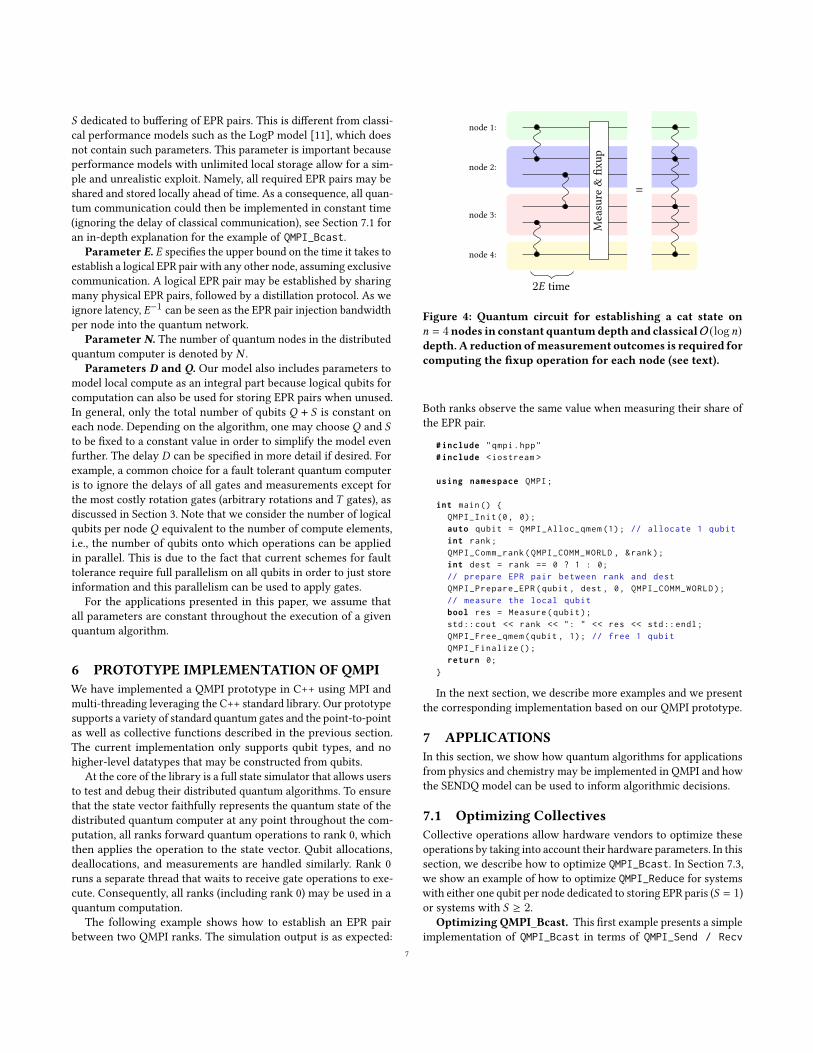
Figure 4: Quantum circuit for establishing a cat state on𝑛 = 4nodes in constant quantumdepth and classicalO(log𝑛)depth. A reduction ofmeasurement outcomes is required forcomputing the fixup operation for each node (see text).

Both ranks observe the same value when measuring their share ofthe EPR pair.

#include "qmpi.hpp"

#include <iostream >

using namespace QMPI;

int main() {

QMPI_Init(0, 0);

auto qubit = QMPI_Alloc_qmem (1); // allocate 1 qubit

int rank;

QMPI_Comm_rank(QMPI_COMM_WORLD , &rank);

int dest = rank == 0 ? 1 : 0;

// prepare EPR pair between rank and dest

QMPI_Prepare_EPR(qubit , dest , 0, QMPI_COMM_WORLD);

// measure the local qubit

bool res = Measure(qubit);

std::cout << rank << ": " << res << std::endl;

QMPI_Free_qmem(qubit , 1); // free 1 qubit

QMPI_Finalize ();

return 0;

}

In the next section, we describe more examples and we presentthe corresponding implementation based on our QMPI prototype.

7 APPLICATIONSIn this section, we show how quantum algorithms for applicationsfrom physics and chemistry may be implemented in QMPI and howthe SENDQ model can be used to inform algorithmic decisions.

7.1 Optimizing CollectivesCollective operations allow hardware vendors to optimize theseoperations by taking into account their hardware parameters. In thissection, we describe how to optimize QMPI_Bcast. In Section 7.3,we show an example of how to optimize QMPI_Reduce for systemswith either one qubit per node dedicated to storing EPR paris (𝑆 = 1)or systems with 𝑆 ≥ 2.

Optimizing QMPI_Bcast. This first example presents a simpleimplementation of QMPI_Bcast in terms of QMPI_Send / Recv

7

and shows how it can be analyzed and optimized using SENDQ.For simplicity, we assume that only one qubit is sent.

A log-depth implementation of broadcast can be achieved byconstructing a binary tree of calls to QMPI_Send / Recv: In the 𝑘-thstep (starting with 𝑘 = 0), 2𝑘 nodes send the broadcast message to1 other node, thus doubling the number of nodes that have receivedthe message at every step. Since each node communicates with (atmost) one node at every step, only one EPR pair must be establishedbetween each pair of nodes that communicates. As a result, 𝑆 = 1is sufficient and the runtime of a broadcast is 𝐸 ⌈log2 𝑁 ⌉.

This implementation may be optimized by realizing that a catstate, which is an 𝑛-qubit generalization of an EPR pair, that is,

|cat(𝑛)⟩ := 1√2( |0 · · · 0︸︷︷︸

𝑛

⟩ + |1 · · · 1︸︷︷︸𝑛

⟩),

can be prepared in constant depth [25]. In QMPI, |cat(𝑛)⟩ can beprepared by first connecting all 𝑛 nodes with EPR pairs along theedges of a spanning tree, and then combining the individual EPRpairs using a parity-measurement of the different EPR pair qubitson each node (no parity-measurement is performed on leaf nodes),see Fig. 4 for a simplified diagram of this process. The measure-ment outcomes are used to compute whether or not a given nodemust apply a Pauli X correction. Specifically, each node 𝑘 applies𝑋𝑟1⊕···⊕𝑟𝑘−1 to the qubit that will be part of the cat state, where 𝑟𝑖denotes the outcome of the (in-place) parity measurement on node𝑖 , and

⊕𝑘−1𝑖=1 𝑟𝑖 can be computed with a classical MPI_Exscan.

This procedure can be extended to an implementation of QMPI_B-cast by also performing a parity measurement between the qubitto broadcast and the one EPR pair qubit on the root node. Thisimplementation runs in quantum time

2𝐸 + 𝐷𝑀 + 𝐷𝐹 ,

where 𝐷𝑀 and 𝐷𝐹 denotes the time it takes to perform a localtwo-qubit parity measurement and to apply an X gate (the fixupoperation), respectively. The classical QMPI_Exscan, which is usedto determine whether or not a local X gate correction is needed,can be performed in O(log𝑁 ) classical communication steps [45].

7.2 Transverse-field Ising modelIn this second example, we show how to simulate the time evolu-tion of a transverse-field Ising model (TFIM) with 𝑛 spins, whoseHamiltonian is given by

𝐻TFIM =∑︁⟨𝑖, 𝑗 ⟩

𝐽𝑖 𝑗𝜎(𝑖)𝑧 𝜎

( 𝑗)𝑧 −

𝑛−1∑︁𝑖=0

Γ𝑖𝜎(𝑖)𝑥 ,

where 𝜎 (𝑖)𝑥 , 𝜎

(𝑖)𝑧 denotes a Pauli X and Z, respectively, acting on

spin index 𝑖 < 𝑛, 𝐽𝑖 𝑗 denotes the coupling constant, and Γ𝑖 is the(local) strength of the transverse field. The first sum runs over allconnected spins 𝑖, 𝑗 , which we denote by ⟨𝑖, 𝑗⟩.

Time evolution under this Hamiltonian can be used as a build-ing block to solve optimization problems leveraging the adiabatictheorem [7]: One first maps the optimization problem to a classicalIsing model (thus defining the connectivity and the parameters 𝐽𝑖 𝑗 ).Then, starting with 𝐽𝑖 𝑗 = 0, Γ𝑖 = 1 and in the ground state of thecorresponding Hamiltonian (which is |+⟩⊗𝑛), one slowly changes

the parameters to Γ𝑖 = 0 and 𝐽𝑖 𝑗 equal to the computed values, aim-ing to remain in the groundstate of all intermediate Hamiltonians.Upon success, a final measurement of all qubits yields the solutionof the optimization problem.

In the following, we assume linear nearest-neighbor connectivityfor the spins and 𝐽𝑖 𝑗 = 𝐽 , Γ𝑖 = Γ for simplicity. The time evolutionoperator for the Hamiltonian 𝐻 is given by 𝑈 (𝑡) = 𝑒−𝑖𝑡𝐻 , where𝑡 is the time to evolve and 𝑖2 = −1. One possible approach toimplement a TFIM simulation on a quantum computer is to firstmap each spin to a qubit. 𝑈 (𝑡) may then be implemented by firstdecomposing it using a Trotter-Suzuki expansion. For example, afirst-order approximation is

𝑈 (𝑡) ≈(𝑒𝑖𝛿𝑡𝐻1𝑒𝑖𝛿𝑡𝐻2

) 𝑡𝛿𝑡

,

for small 𝛿𝑡 and 𝐻1 := −𝐽 ∑⟨𝑖, 𝑗 ⟩ 𝜎(𝑖)𝑧 𝜎

( 𝑗)𝑧 , 𝐻2 := Γ

∑𝑖 𝜎

(𝑖)𝑥 . The

individual terms in 𝐻1 commute, and so do the terms within 𝐻2.Therefore,

𝑒−𝑖𝛿𝑡𝐻1 =∏⟨𝑖, 𝑗 ⟩

𝑒−𝑖𝛿𝑡 𝐽 𝜎(𝑖 )𝑧 𝜎

( 𝑗 )𝑧 , and 𝑒−𝑖𝛿𝑡𝐻2 =

∏𝑖

𝑒𝑖𝛿𝑡Γ𝜎(𝑖 )𝑥 .

Each term in the first product can be implemented by computingthe parity between spin 𝑖 and 𝑗 using a CNOT gate, followed by arotation gate 𝑅𝑧 (\ ) = 𝑒−0.5𝑖\𝜎𝑧 and another CNOT gate to uncom-pute the parity. The terms in the second product are just rotationgates 𝑅𝑥 (\ ) = 𝑒−0.5𝑖\𝜎𝑥 acting on qubit 𝑖 .

The complete code for the simulation can be found in the ap-pendix, see Listing 1. While the prototype implementation usesblocking send/receive calls, we note that one would use an asyn-chronous version in practice: The EPR pairs could be establishedwhile applying the local operations.

Analysis with SENDQ. Each Trotter step requires 𝑁 EPR pairs,where 𝑁 denotes the number of nodes, and each node prepares anEPR pair with the two nodes that contain adjacent spins. We assumethat rotation gates cannot be executed in parallel due to the cost(in space) of 𝑇 -state factories. Since the delay of each rotation gate𝐷𝑅 is much larger than the logical gate time, we ignore the cost ofCNOTs. As a result, the delay of one Trotter step is approximately

𝐷Trotter = 2𝑛

𝑁𝐷𝑅 = 2𝑄𝐷𝑅,

assuming that 𝑛 is divisible by 𝑁 .To ensure that communication is not a bottleneck (assuming

asynchronous send/receive implementations), the time spent onlocal gates should be at least as large as the time it takes to establishtwo EPR pairs. For 𝑆 ≥ 2, this means that

𝐷Trotter ≥ 2𝐸.

In turn, this allows us to inform our choice of the number ofnodes 𝑁 if sufficient space is available per node to temporarily storethe two EPR pairs: 𝑁 should be chosen such that

𝐸−1𝑛𝐷𝑅 ≥ 𝑁 .

If, on the other hand, space per node is a limiting factor and 𝑆 = 1while 𝑄 ≥ 2, then one may return to the 𝑆 ≥ 2 case by increasingthe number of nodes to 𝑁 ≥ ⌈ 𝑛

𝑄−1 ⌉.We now address the case where increasing the number of nodes

is not an option. Specifically, we show that our model correctly8

predicts an overhead for 𝑆 = 1 compared to 𝑆 ≥ 2 even with anoptimized communication schedule that allows for halting localcomputations at any point, e.g., during execution of a local rotationgate. With 𝑆 = 1, a request for EPR pair creation can only be initi-ated once the buffer qubit has been cleared. As a result, there is anadditional delay𝐷𝑅 between EPR pair creation requests because therotation must be applied before the remote qubit can be unreceived.The delay per Trotter step with an optimized schedule for initiatingEPR pair creation requests is thus

max (𝐷Trotter, 2𝐸 + 2𝐷𝑅) ,in contrast to the 𝑆 ≥ 2 case, where the delay per Trotter step ismax (𝐷Trotter, 2𝐸).

This TFIM example shows that SENDQ can be used to modelvarious tradeoffs in the implementation of a distributed quantumalgorithm. Crucially, smaller 𝑆 results in longer runtimes, even ifthe communication schedule is optimized.

7.3 ChemistrySimulation of molecules is currently one of the most promisingapplications to first show a quantum advantage for a practical prob-lem compared to classical supercomputers. The goal is to determinethe energy eigenstates of molecules described by a Hamiltonian 𝐻 .This then allows, for example, to investigate and optimize chemicalcatalysis [57].

For large molecules the best quantum algorithms to find groundstate energies are based on phase estimation of a unitary operatorwhich depends only on the Hamiltonian of the molecule 𝐻 . For agiven molecule, the full quantum circuit is known at circuit compi-lation time, i.e., there are no branches in the program dependingto measurements during runtime which influence performance.Hence, one can use expensive quantum circuit optimization tech-niques to reduce the quantum resources and increase performanceahead of time. We will highlight a few optimization possibilities fora distributed quantum computer.

We consider the algorithm of expressing the Hamiltonian 𝐻

of a molecule of interest in second quantization, expressed in abasis of 𝑛 spin-orbitals. This algorithm requires at least 𝑛 dataqubits which might be distributed onto different nodes. We performphase estimation on the time evolution operator of the system,𝑒−𝑖𝑡𝐻 , which we implement using a Trotter-Suzuki expansion fromSection 7.2. The majority of the algorithm is only one primitiveoperation, namely, a time evolution operator of the form:

𝑒−𝑖𝑡𝑍𝑖1𝑍𝑖2 · · ·𝑍𝑖𝑘 , {𝑖1, . . . , 𝑖𝑘 } ⊆ {0, . . . , 𝑛 − 1}, 𝑡 ∈ R. (1)

The qubit indices and parameter 𝑡 involved in each of these opera-tors depend on the molecule and on the choices of how to representits Hamiltonian.

Analysis with SENDQ. For a given molecule to be simulated,there are several choices to be made when mapping the problem toa quantum computer. In particular, different choices lead to differ-ent Hamiltonians, even if they all describe the same molecule. Forexample, the fermionic Hamiltonian needs to be transformed intoa Hamiltonian that acts on qubits. This can be achieved using theJordan-Wigner transformation [27, 42, 49], the Bravyi-Kitaev en-coding [9], or by using more than 𝑛 data qubits [61]. For example, aJordan-Wigner transformation will result in operations as in Eq. (1),

0 10 20 30 40 50 60

Number of qubits per term

100

101

102

103

104

105

Num

ber

of

term

s

Jordan-Wigner

Bravyi-Kitaev

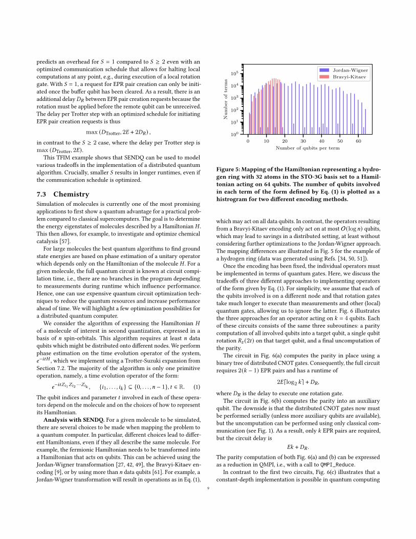
Figure 5: Mapping of the Hamiltonian representing a hydro-gen ring with 32 atoms in the STO-3G basis set to a Hamil-tonian acting on 64 qubits. The number of qubits involvedin each term of the form defined by Eq. (1) is plotted as ahistrogram for two different encoding methods.

which may act on all data qubits. In contrast, the operators resultingfrom a Bravyi-Kitaev encoding only act on at most O(log𝑛) qubits,which may lead to savings in a distributed setting, at least withoutconsidering further optimizations to the Jordan-Wigner approach.The mapping differences are illustrated in Fig. 5 for the example ofa hydrogen ring (data was generated using Refs. [34, 50, 51]).

Once the encoding has been fixed, the individual operators mustbe implemented in terms of quantum gates. Here, we discuss thetradeoffs of three different approaches to implementing operatorsof the form given by Eq. (1). For simplicity, we assume that each ofthe qubits involved is on a different node and that rotation gatestake much longer to execute than measurements and other (local)quantum gates, allowing us to ignore the latter. Fig. 6 illustratesthe three approaches for an operator acting on 𝑘 = 4 qubits. Eachof these circuits consists of the same three subroutines: a paritycomputation of all involved qubits into a target qubit, a single qubitrotation 𝑅𝑧 (2𝑡) on that target qubit, and a final uncomputation ofthe parity.

The circuit in Fig. 6(a) computes the parity in place using abinary tree of distributed CNOT gates. Consequently, the full circuitrequires 2(𝑘 − 1) EPR pairs and has a runtime of

2𝐸 ⌈log2 𝑘⌉ + 𝐷𝑅,

where 𝐷𝑅 is the delay to execute one rotation gate.The circuit in Fig. 6(b) computes the parity into an auxiliary

qubit. The downside is that the distributed CNOT gates now mustbe performed serially (unless more auxiliary qubits are available),but the uncomputation can be performed using only classical com-munication (see Fig. 1). As a result, only 𝑘 EPR pairs are required,but the circuit delay is

𝐸𝑘 + 𝐷𝑅 .

The parity computation of both Fig. 6(a) and (b) can be expressedas a reduction in QMPI, i.e., with a call to QMPI_Reduce.

In contrast to the first two circuits, Fig. 6(c) illustrates that aconstant-depth implementation is possible in quantum computing

9

𝑞0

𝑞1

𝑞2

𝑞3

𝑅𝑧 (2𝑡)

(a) In-place

𝑞0

𝑞1

𝑞2

𝑞3

|0⟩ 𝑅𝑧 (2𝑡) 𝐻

𝑍 ⊗4

(b) Out-of-place

𝑞0

𝑞1

𝑞2

𝑞3

|0⟩

𝐻

𝐻

𝐻

𝐻

𝐻

𝐻

𝐻

𝐻

𝐻

𝐻 𝑅𝑧 (2𝑡) 𝐻

𝑍 ⊗4

(c) Constant-depth

Figure 6: Three different methods to implement𝑒−𝑖𝑡𝑍0𝑍1 · · ·𝑍𝑘−1 for 𝑘 = 4.

using a parallel implementation of the multi-target CNOT. Specifi-cally, this involves fanning out the control qubit using QMPI_Bcastto each node, which requires 𝑘 EPR pairs to establish a cat state,see Section 7.1, and, thus, 𝑆 ≥ 2 is needed [25, 28]. The delay ofthis constant-depth implementation is

2𝐸 + 𝐷𝑅 .

As the full quantum circuit is known at circuit generation time,a compiler may choose the optimal method for each term, giventhe available resources at that point in the program. See Fig. 7for an example of a straight forward implementation without anyadvanced optimization applied to it.

8 CONCLUSIONS AND OUTLOOKWe introduce QMPI, an extension of MPI to distibuted quantumcomputing. This enables the development of portable high-per-formance distributed quantum programs. Complementary, we in-troduce the machine-independent SENDQ performance model fordistributed quantum computing. The model is motivated by tech-nological trends in building large-scale fault-tolerant quantum ma-chines. These considerations allowed us to simplify the model by,e.g., not modeling the overhead due to classical communication asthe clock cycle rate of logical quantum operations is expected to besignificantly lower. As a consequence, we end up with a deliberatelysimple model with only a small set of general parameters.

12 4 8 16 32 64

Number of nodes

0.00

0.25

0.50

0.75

1.00

1.25

1.50

Num

ber

of

EP

Rpair

s

×107

BK (in-place)

BK (const.-depth)

JW (in-place)

JW (const.-depth)

Figure 7: Number of EPR pairs required for communicationto simulate one first-order Trotter step for a hydrogen ringof 32 atoms in the STO-3G basis set as a function of thenumber of nodes. We used either the Bravyi-Kitaev (BK) orthe Jordan-Wigner (JW) encoding, see also Fig. 5. One im-plementation uses the in-place circuit of Fig. 6(a) which wecompare to the circuit in Fig. 6(c). The constant-depth cir-cuit requires more local resources such as 𝑆 ≥ 2 and we addi-tionally assumed that the rotation can be performed on anauxiliary qubit on one of the nodes already storing one ofthe involved orbitals. We did not consider advanced optimi-sations and the spin-orbitals are fixed in our example to aspecific node for the full duration.

The SENDQ model thus allows us to expose different tradeoffsof distributed quantum algorithms in a machine-agnostic fashionand without having to deal with unnecessary details. We illustrateuse cases from quantum chemistry and from condensed matterphysics. Our model encourages algorithm designers to start think-ing about qubit placement in a distributed setting, and overlayingcommunication with local computation.

The high-level modeling of the quantum network without speci-fying details allows hardware developers to explore implementationchoices such as different quantum network topologies, and to quan-tify their impact in terms of the effect on the runtime of large-scalequantum computing applications.

ACKNOWLEDGMENTSWe thank Vadym Kliuchnikov for helpful discussions. This projectreceived support from the Microsoft Swiss Joint Research Center.

REFERENCES[1] Gadi Aleksandrowicz, Thomas Alexander, Panagiotis Barkoutsos, Luciano Bello,

Yael Ben-Haim, D Bucher, FJ Cabrera-Hernández, J Carballo-Franquis, A Chen,CF Chen, et al. 2019. Qiskit: An open-source framework for quantum computing.Accessed on: Mar 16 (2019).

[2] David Awschalom, Karl K. Berggren, Hannes Bernien, Sunil Bhave, Lincoln D.Carr, Paul Davids, Sophia E. Economou, Dirk Englund, Andrei Faraon, MartinFejer, Saikat Guha, Martin V. Gustafsson, Evelyn Hu, Liang Jiang, JungsangKim, Boris Korzh, Prem Kumar, Paul G. Kwiat, Marko Lončar, Mikhail D. Lukin,David A.B. Miller, Christopher Monroe, Sae Woo Nam, Prineha Narang, Jason S.Orcutt, Michael G. Raymer, Amir H. Safavi-Naeini, Maria Spiropulu, Kartik Srini-vasan, Shuo Sun, Jelena Vučković, Edo Waks, Ronald Walsworth, Andrew M.

10

Weiner, and Zheshen Zhang. 2021. Development of Quantum Interconnects(QuICs) for Next-Generation Information Technologies. PRX Quantum 2 (Feb2021), 017002. Issue 1. https://doi.org/10.1103/PRXQuantum.2.017002

[3] Robert Beals, Stephen Brierley, Oliver Gray, Aram W Harrow, Samuel Kutin,Noah Linden, Dan Shepherd, and Mark Stather. 2013. Efficient distributed quan-tum computing. Proceedings of the Royal Society A: Mathematical, Physical andEngineering Sciences 469, 2153 (2013), 20120686.

[4] Charles H Bennett. 1973. Logical reversibility of computation. IBM journal ofResearch and Development 17, 6 (1973), 525–532.

[5] Charles H. Bennett, Gilles Brassard, Sandu Popescu, Benjamin Schumacher,John A. Smolin, and William K. Wootters. 1996. Purification of Noisy Entangle-ment and Faithful Teleportation via Noisy Channels. Phys. Rev. Lett. 76 (Jan 1996),722–725. Issue 5. https://doi.org/10.1103/PhysRevLett.76.722

[6] Benjamin Bichsel, Maximilian Baader, Timon Gehr, and Martin Vechev. 2020. Silq:A high-level quantum language with safe uncomputation and intuitive semantics.In Proceedings of the 41st ACM SIGPLAN Conference on Programming LanguageDesign and Implementation. 286–300.

[7] Max Born and Vladimir Fock. 1928. Beweis des adiabatensatzes. Zeitschrift fürPhysik 51, 3-4 (1928), 165–180.

[8] Sergey Bravyi and Alexei Kitaev. 2005. Universal quantum computation withideal Clifford gates and noisy ancillas. Physical Review A 71, 2 (2005), 022316.

[9] Sergey B. Bravyi and Alexei Yu. Kitaev. 2002. Fermionic Quantum Computation.Annals of Physics 298, 1 (2002), 210–226. https://doi.org/10.1006/aphy.2002.6254

[10] Daniel Collins, Noah Linden, and Sandu Popescu. 2001. Nonlocal content ofquantum operations. Phys. Rev. A 64 (Aug 2001), 032302. Issue 3. https://doi.org/10.1103/PhysRevA.64.032302

[11] David Culler, Richard Karp, David Patterson, Abhijit Sahay, Klaus Erik Schauser,Eunice Santos, Ramesh Subramonian, and Thorsten Von Eicken. 1993. LogP:Towards a realistic model of parallel computation. In Proceedings of the fourthACM SIGPLAN symposium on Principles and practice of parallel programming.1–12.

[12] Axel Dahlberg, Matthew Skrzypczyk, Tim Coopmans, Leon Wubben, FilipRozpędek, Matteo Pompili, Arian Stolk, Przemysław Pawełczak, Robert Knegjens,Julio de Oliveira Filho, et al. 2019. A link layer protocol for quantum networks. InProceedings of the ACM Special Interest Group on Data Communication. 159–173.

[13] Axel Dahlberg and Stephanie Wehner. 2018. SimulaQron—a simulator for devel-oping quantum internet software. Quantum Science and Technology 4, 1 (2018),015001.

[14] Sebastian Debone, Runsheng Ouyang, Kenneth Goodenough, and David Elkouss.2020. Protocols for creating and distilling multipartite GHZ states with Bell pairs.IEEE Transactions on Quantum Engineering (2020).

[15] Stephen DiAdamo, Marco Ghibaudi, and James Cruise. 2021. Dis-tributed Quantum Computing and Network Control for Accelerated VQE.arXiv:2101.02504 [quant-ph]

[16] A. Einstein, B. Podolsky, and N. Rosen. 1935. Can Quantum-Mechanical De-scription of Physical Reality Be Considered Complete? Phys. Rev. 47 (May 1935),777–780. Issue 10. https://doi.org/10.1103/PhysRev.47.777

[17] J. Eisert, K. Jacobs, P. Papadopoulos, and M. B. Plenio. 2000. Optimal localimplementation of nonlocal quantum gates. Phys. Rev. A 62 (Oct 2000), 052317.Issue 5. https://doi.org/10.1103/PhysRevA.62.052317

[18] Moritz Forsch, Robert Stockill, AndreasWallucks, Igor Marinković, Claus Gärtner,Richard A Norte, Frank van Otten, Andrea Fiore, Kartik Srinivasan, and SimonGröblacher. 2020. Microwave-to-optics conversion using a mechanical oscillatorin its quantum ground state. Nature Physics 16, 1 (2020), 69–74.

[19] Jay Gambetta. 2020. IBM’s Roadmap For Scaling Quantum Technology. https://www.ibm.com/blogs/research/2020/09/ibm-quantum-roadmap/. Accessed:16.03.2021.

[20] Craig Gidney and Martin Ekerå. 2019. How to factor 2048 bit rsa integers in 8hours using 20 million noisy qubits. arXiv preprint arXiv:1905.09749 (2019).

[21] Alexander S Green, Peter LeFanu Lumsdaine, Neil J Ross, Peter Selinger, andBenoît Valiron. 2013. Quipper: a scalable quantum programming language. InProceedings of the 34th ACM SIGPLAN conference on Programming language designand implementation. 333–342.

[22] Thomas Häner, Samuel Jaques, Michael Naehrig, Martin Roetteler, and MathiasSoeken. 2020. Improved quantum circuits for elliptic curve discrete logarithms.In International Conference on Post-Quantum Cryptography. Springer, 425–444.

[23] Torsten Hoefler, Prabhanjan Kambadur, Richard L Graham, Galen Shipman,and Andrew Lumsdaine. 2007. A case for standard non-blocking collectiveoperations. In European Parallel Virtual Machine/Message Passing Interface Users’Group Meeting. Springer, 125–134.

[24] Julian Hofmann, Michael Krug, Norbert Ortegel, Lea Gérard, MarkusWeber, Wenjamin Rosenfeld, and Harald Weinfurter. 2012. Her-alded Entanglement Between Widely Separated Atoms. Science337, 6090 (2012), 72–75. https://doi.org/10.1126/science.1221856arXiv:https://science.sciencemag.org/content/337/6090/72.full.pdf

[25] Peter Høyer and Robert Špalek. 2005. Quantum fan-out is powerful. Theory ofcomputing 1, 1 (2005), 81–103.

[26] Ali JavadiAbhari, Shruti Patil, Daniel Kudrow, JeffHeckey, Alexey Lvov, Frederic TChong, andMargaret Martonosi. 2015. ScaffCC: Scalable compilation and analysisof quantum programs. Parallel Comput. 45 (2015), 2–17.

[27] P. Jordan and E. Wigner. 1928. Über das Paulische Äquivalenzverbot. Zeitschriftfür Physik 47, 9 (1928), 631–651. https://doi.org/10.1007/BF01331938

[28] Vadym Kliuchnikov and Alexander Vaschillo. 2021. Layout based on cat states.In preparation (2021).

[29] Joonho Lee, Dominic Berry, Craig Gidney, William J Huggins, Jarrod R Mc-Clean, Nathan Wiebe, and Ryan Babbush. 2020. Even more efficient quantumcomputations of chemistry through tensor hypercontraction. arXiv preprintarXiv:2011.03494 (2020).

[30] Bjoern Lekitsch, Sebastian Weidt, Austin G Fowler, Klaus Mølmer, Simon J Devitt,Christof Wunderlich, andWinfried K Hensinger. 2017. Blueprint for a microwavetrapped ion quantum computer. Science Advances 3, 2 (2017), e1601540.

[31] Daniel Litinski. 2019. Magic state distillation: Not as costly as you think. Quantum3 (2019), 205.

[32] Paul Magnard, Simon Storz, Philipp Kurpiers, Josua Schär, Fabian Marxer, JanisLütolf, T Walter, J-C Besse, M Gabureac, K Reuer, et al. 2020. Microwave quantumlink between superconducting circuits housed in spatially separated cryogenicsystems. Physical Review Letters 125, 26 (2020), 260502.

[33] Sam McArdle, Suguru Endo, Alán Aspuru-Guzik, Simon C. Benjamin, and XiaoYuan. 2020. Quantum computational chemistry. Rev. Mod. Phys. 92 (Mar 2020),015003. Issue 1. https://doi.org/10.1103/RevModPhys.92.015003

[34] Jarrod R McClean, Nicholas C Rubin, Kevin J Sung, Ian D Kivlichan, Xavier Bonet-Monroig, Yudong Cao, Chengyu Dai, E Schuyler Fried, Craig Gidney, BrendanGimby, et al. 2020. OpenFermion: the electronic structure package for quantumcomputers. Quantum Science and Technology 5, 3 (2020), 034014.

[35] Rodney Van Meter, WJ Munro, Kae Nemoto, and Kohei M Itoh. 2008. Arithmeticon a distributed-memory quantum multicomputer. ACM Journal on EmergingTechnologies in Computing Systems (JETC) 3, 4 (2008), 1–23.

[36] Rodney Doyle Van Meter III. 2006. Architecture of a quantum multicomputeroptimized for shor’s factoring algorithm. arXiv preprint quant-ph/0607065 (2006).

[37] David L Moehring, Peter Maunz, Steve Olmschenk, Kelly C Younge, Dzmitry NMatsukevich, L-M Duan, and Christopher Monroe. 2007. Entanglement of single-atom quantum bits at a distance. Nature 449, 7158 (2007), 68–71.

[38] C. Monroe, R. Raussendorf, A. Ruthven, K. R. Brown, P. Maunz, L.-M. Duan, andJ. Kim. 2014. Large-scale modular quantum-computer architecture with atomicmemory and photonic interconnects. Phys. Rev. A 89 (Feb 2014), 022317. Issue 2.https://doi.org/10.1103/PhysRevA.89.022317

[39] Hartmut Neven. 2020. Google Quantum AI updates at Quantum Summer Sympo-sium 2020. https://www.youtube.com/watch?v=TJ6vBNEQReU Online; posted3-September-2020, accessed 25-March-2021.

[40] Naomi H. Nickerson, Joseph F. Fitzsimons, and Simon C. Benjamin. 2014. FreelyScalable Quantum Technologies Using Cells of 5-to-50 Qubits with Very Lossyand Noisy Photonic Links. Phys. Rev. X 4 (Dec 2014), 041041. Issue 4. https://doi.org/10.1103/PhysRevX.4.041041

[41] Michael A Nielsen and Isaac Chuang. 2002. Quantum computation and quantuminformation.

[42] Gerardo Ortiz, James E Gubernatis, Emanuel Knill, and Raymond Laflamme. 2001.Quantum algorithms for fermionic simulations. Physical Review A 64, 2 (2001),022319.

[43] Stefano Pirandola, Ulrik L Andersen, Leonardo Banchi, Mario Berta, DariusBunandar, Roger Colbeck, Dirk Englund, Tobias Gehring, Cosmo Lupo, CarloOttaviani, et al. 2020. Advances in quantum cryptography. Advances in Opticsand Photonics 12, 4 (2020), 1012–1236.

[44] Markus Reiher, NathanWiebe, KrystaM Svore, DaveWecker, andMatthias Troyer.2017. Elucidating reaction mechanisms on quantum computers. Proceedings ofthe National Academy of Sciences 114, 29 (2017), 7555–7560.

[45] Peter Sanders and Jesper Larsson Träff. 2006. Parallel prefix (scan) algorithms forMPI. In European Parallel Virtual Machine/Message Passing Interface Users’ GroupMeeting. Springer, 49–57.

[46] VM Schäfer, CJ Ballance, K Thirumalai, LJ Stephenson, TG Ballance, AM Steane,and DM Lucas. 2018. Fast quantum logic gates with trapped-ion qubits. Nature555, 7694 (2018), 75–78.

[47] Artur Scherer, Benoît Valiron, Siun-Chuon Mau, Scott Alexander, Eric Van denBerg, and Thomas E Chapuran. 2017. Concrete resource analysis of the quantumlinear-system algorithm used to compute the electromagnetic scattering crosssection of a 2D target. Quantum Information Processing 16, 3 (2017), 1–65.

[48] Peter W Shor. 1994. Algorithms for quantum computation: discrete logarithmsand factoring. In Proceedings 35th annual symposium on foundations of computerscience. Ieee, 124–134.

[49] Rolando Somma, GerardoOrtiz, James EGubernatis, Emanuel Knill, and RaymondLaflamme. 2002. Simulating physical phenomena by quantum networks. PhysicalReview A 65, 4 (2002), 042323.

[50] Damian S Steiger, Thomas Häner, and Matthias Troyer. 2018. ProjectQ: an opensource software framework for quantum computing. Quantum 2 (2018), 49.

[51] Qiming Sun, Timothy C. Berkelbach, Nick S. Blunt, George H. Booth, ShengGuo, Zhendong Li, Junzi Liu, James D. McClain, Elvira R. Sayfutyarova, Sandeep

11

Sharma, Sebastian Wouters, and Garnet Kin-Lic Chan. 2017. PySCF: the Python-based simulations of chemistry framework. , e1340 pages. https://doi.org/10.1002/wcms.1340 arXiv:https://onlinelibrary.wiley.com/doi/pdf/10.1002/wcms.1340

[52] Krysta Svore, Alan Geller, Matthias Troyer, John Azariah, Christopher Granade,Bettina Heim, Vadym Kliuchnikov, Mariia Mykhailova, Andres Paz, and MartinRoetteler. 2018. Q# enabling scalable quantum computing and developmentwith a high-level dsl. In Proceedings of the Real World Domain Specific LanguagesWorkshop 2018. 1–10.

[53] Yuta Tsuchimoto, Patrick Knüppel, Aymeric Delteil, Zhe Sun, Martin Kroner,and Ata ç Imamoğlu. 2017. Proposal for a quantum interface between photonicand superconducting qubits. Phys. Rev. B 96 (Oct 2017), 165312. Issue 16. https://doi.org/10.1103/PhysRevB.96.165312

[54] S. J. van Enk, J. I. Cirac, and P. Zoller. 1997. Ideal Quantum Communication overNoisy Channels: A Quantum Optical Implementation. Phys. Rev. Lett. 78 (Jun1997), 4293–4296. Issue 22. https://doi.org/10.1103/PhysRevLett.78.4293

[55] Rodney Van Meter and Simon J Devitt. 2016. The path to scalable distributedquantum computing. Computer 49, 9 (2016), 31–42.

[56] Rod Van Meter, Kae Nemoto, and W Munro. 2007. Communication links fordistributed quantum computation. IEEE Trans. Comput. 56, 12 (2007), 1643–1653.

[57] Vera von Burg, Guang Hao Low, Thomas Häner, Damian S Steiger, Markus Reiher,Martin Roetteler, and Matthias Troyer. 2020. Quantum computing enhancedcomputational catalysis. arXiv preprint arXiv:2007.14460 (2020).

[58] David W Walker and Jack J Dongarra. 1996. MPI: a standard message passinginterface. Supercomputer 12 (1996), 56–68.

[59] Adam Bene Watts, Robin Kothari, Luke Schaeffer, and Avishay Tal. 2019. Ex-ponential Separation between Shallow Quantum Circuits and Unbounded Fan-in Shallow Classical Circuits. In Proceedings of the 51st Annual ACM SIGACTSymposium on Theory of Computing (Phoenix, AZ, USA) (STOC 2019). As-sociation for Computing Machinery, New York, NY, USA, 515–526. https://doi.org/10.1145/3313276.3316404

[60] Stephanie Wehner, David Elkouss, and Ronald Hanson. 2018. Quantum internet:A vision for the road ahead. Science 362, 6412 (2018).

[61] James D. Whitfield, Vojt ěch Havlíček, and Matthias Troyer. 2016. Local spinoperators for fermion simulations. Phys. Rev. A 94 (Sep 2016), 030301. Issue 3.https://doi.org/10.1103/PhysRevA.94.030301

[62] Ze-Liang Xiang, Mengzhen Zhang, Liang Jiang, and Peter Rabl. 2017. Intracityquantum communication via thermal microwave networks. Physical Review X 7,1 (2017), 011035.

[63] Anocha Yimsiriwattana and Samuel J Lomonaco Jr. 2004. Distributed quantumcomputing: A distributed Shor algorithm. In Quantum Information and Computa-tion II, Vol. 5436. International Society for Optics and Photonics, 360–372.

[64] Anocha Yimsiriwattana and Samuel J Lomonaco Jr. 2004. Generalized GHZ statesand distributed quantum computing. arXiv preprint quant-ph/0402148 (2004).

[65] Youpeng Zhong, Hung-Shen Chang, Audrey Bienfait, Étienne Dumur, Ming-HanChou, Christopher R Conner, Joel Grebel, Rhys G Povey, Haoxiong Yan, David ISchuster, et al. 2021. Deterministic multi-qubit entanglement in a quantumnetwork. Nature 590, 7847 (2021), 571–575.

A EXAMPLE IMPLEMENTATIONSA.1 Moving QubitsHere, we give an example implementation of QMPI_Send_moveand QMPI_Recv_move in our QMPI prototype. The sender executesQMPI_Send_move, which sends a qubit (with move semantics), andthe receiver calls the corresponding QMPI_Recv_move. Both of thesefunctions can be implemented using EPR-pair preparation and localquantum operations as follows:

void QMPI_Send_move(QMPI_QUBIT_PTR qubit , int dest , inttag , MPI_Comm comm) {

auto epr_qubit = QMPI_Alloc_qmem (1);

QMPI_Prepare_EPR(epr_qubit , dest , tag , comm);

CNOT(qubit , epr_qubit);

int r=0;

r = Measure(epr_qubit);

H(qubit);

r |= 2 * Measure(qubit);

QMPI_Free_qmem(epr_qubit , 1);

MPI_Send (&r, 1, MPI_INT , dest , tag , comm);

}

void QMPI_Recv_move(QMPI_QUBIT_PTR qubit , int src , inttag , MPI_Comm comm) {

QMPI_Prepare_EPR(qubit , src , tag , comm);

int r;

MPI_Recv (&r, 1, MPI_INT , src , tag , comm ,

MPI_STATUS_IGNORE);

if (r&1)

X(qubit);

if (r&2)

Z(qubit);

}

We note that these functions may also be implemented by rely-ing on QMPI_Send / Recv and their inverses: Once the value of aqubit is shared between two nodes, it is no longer possible to distin-guish sender from receiver. Therefore, the two involved nodes mayexchange roles when calling the inverses of QMPI_Send / Recv,resulting in a slightly less efficient implementation of teleportation(since measurement results are communicated using two one-bitmessages instead of one two-bit message).

A.2 Transverse-field Ising Model (TFIM).As a second code example, we provide an implementation of timeevolution under a TFIM Hamiltonian below. Note that the codealso includes annealing from a fully transverse-field model to afully classical Ising model. We note that the code can be signifi-cantly optimized by using asynchronous communication primitives.However, we use blocking calls only to simplify the presentation.

#include "qmpi.hpp"

#include <iostream >

using namespace QMPI;

void tfim_time_evolution(double const& J, double const&g, double const& time , QMPI_QUBIT_PTR qubits ,

unsigned num_spins , unsigned num_trotter) {

int rank , size;

QMPI_Comm_size(QMPI_COMM_WORLD , &size);

QMPI_Comm_rank(QMPI_COMM_WORLD , &rank);

auto dt = time/num_trotter;

for (unsigned step =0; step < num_trotter; ++step) {

for (unsigned site = 0; site < num_spins -1; ++site)

{

CNOT(qubits+site , qubits+site +1);

Rz(qubits+site+1, 2.0 * J * dt);

CNOT(qubits+site , qubits+site +1);

}

if (size == 1) { // single rank: no communication

required

CNOT(qubits+num_spins -1, qubits);

Rz(qubits , 2.0 * J * dt);

CNOT(qubits+num_spins -1, qubits);

}

else {

for (unsigned odd = 0; odd < 2; ++odd) {

if ((rank &1) == odd) {

QMPI_Send(qubits , (rank -1+ size)%size , 0,

QMPI_COMM_WORLD);

QMPI_Unsend(qubits , (rank -1+ size)%size , 0,

QMPI_COMM_WORLD);

}

else {

auto tmpqubit = QMPI_Alloc_qmem (1);

QMPI_Recv(tmpqubit , (rank +1)%size , 0,

QMPI_COMM_WORLD);

CNOT(qubits+num_spins -1, tmpqubit);

Rz(tmpqubit , 2.0 * J * dt);

CNOT(qubits+num_spins -1, tmpqubit);

12

QMPI_Unrecv(tmpqubit , (rank +1)%size , 0,

QMPI_COMM_WORLD);

QMPI_Free_qmem(tmpqubit , 1);

}

}

}

for (unsigned site = 0; site < num_spins; ++site)

Rx(qubits+site , -2.0*g*dt);

}

}

int main() {

QMPI_Init(0, 0);

int rank , size;

QMPI_Comm_size(QMPI_COMM_WORLD , &size);

QMPI_Comm_rank(QMPI_COMM_WORLD , &rank);

// Number of spins per node:

unsigned num_local_spins = 2;

// Number of annealing steps:

double num_annealing_steps = 100;

// Trotter number

unsigned num_trotter = 1;

double time = 1; // time to evolve per annealing step

// Parameters of transverse -field Ising model

double J = 0.; // coupling strength

double g = 1.; // transverse field

// allocate spins:

auto qubits = QMPI_Alloc_qmem(num_local_spins);

// init to ground state

for (unsigned i = 0; i < num_local_spins; ++i)

H(qubits+i);

// run annealing schedule

for (unsigned step = 0; step < num_annealing_steps;

++step) {

J = step * 1.0/ num_annealing_steps;

g = 1.0-J;

tfim_time_evolution(J, g, time , qubits ,

num_local_spins , num_trotter);

}

// Measure

std::vector <int > res(num_local_spins);

for (unsigned i = 0; i < num_local_spins; ++i)

res[i] = Measure(qubits+i);

QMPI_Free_qmem(qubits , num_local_spins);

// Gather all (classical) results and output

std::vector <int > allres(num_local_spins*size);

MPI_Gather (&res[0], num_local_spins , MPI_INT , &allres

[0], num_local_spins , MPI_INT , 0, QMPI_COMM_WORLD)

;

if (rank == 0) {

std::cout << "Measurements: ";

for (auto r : allres)

std::cout << r << " ";

std::cout << std::endl;

}

QMPI_Finalize ();

return 0;

}

Listing 1: QMPI code for TFIM time evolution and annealing.

13