distributed people counting using a wireless sensor network
TRANSCRIPT

Research Collection
Student Paper
Distributed People Counting Using a Wireless Sensor Network
Author(s): Senti, Patrick
Publication Date: 2011
Permanent Link: https://doi.org/10.3929/ethz-a-009935810
Rights / License: In Copyright - Non-Commercial Use Permitted
This page was generated automatically upon download from the ETH Zurich Research Collection. For moreinformation please consult the Terms of use.
ETH Library

Distributed Computing
Distributed People CountingUsing a Wireless Sensor Network
Semester Thesis
Patrick Senti
patricksenti at student.ethz.ch
Distributed Computing Group
Computer Engineering and Networks Laboratory
ETH Zurich
Supervisors:
Philipp Sommer
Prof. Dr. Roger Wattenhofer
February 2011 - August 2011

ii
Acknowledgements
This thesis would not have been possible without the support by Philipp Sommer andProf. Dr. Roger Wattenhofer, who provided me the opportunity to engage in this work.I thank Philipp Sommer for supporting my initial idea that lead to this thesis, and forhis valuable feedback to intermediary results and to the draft of this report. He alsoprovided helpful insights to implement a functional hardware/software prototype of thepeople-counting sensor node. I am thankful to Prof. Dr. Roger Wattenhofer for theopportunity to complement my studies programme, CAS in Computer Science (Dis-tributed Systems), by this work and in the focus area of his research group.

iv
Abstract
People observation and counting is of interest in many commercial and non-commercialscenarios. The number of people entering and leaving shops, the occupancy of officebuildings or the passenger count of commuter trains provide useful information to shopmerchants and marketers, security officials or train operators. To this end, this thesisdevelops a distributed people counting system, covering algorithms and their imple-mentation on wireless sensor nodes.
The algorithms presented address the people counting problem by interpreting theinfrared sensor signal as system state. In particular, a dynamically configurable FSM isproposed based on regular expressions. In combination with several parameters relatedto sensor signal patterns the algorithms are adjustable to a range of deployment sce-narios. The algorithms are provided as both a simulation model and the correspondingsensor node implementation.
The prototype implementation provides a setup where each sensor node is equippedwith one passive, dual-element infrared sensor (PIR). For evaluation, a prototyping pro-cessor board and low-cost PIR sensors were used to build two wireless sensor nodesfrom commercially available components. A feature of this implementation is that eachsensor node is able to count, on-system and in real-time, the number of passers-by goingin each direction, while requiring relatively little compute power.
A wireless sensor network is described to monitor the count values of distributednodes and collect these data at a base station. The base station transmits the count datato a web-based data collection server, where it can be made available for further useto applications and client devices, such as smartphones. To enable the configuration ofthe sensor nodes to specific installation scenarios, and for the purpose of performanceanalysis, a validation framework is presented.
A stochastic state estimation model is considered to resolve the problem of rela-tively noisy people count measurements by sensors. In particular, the Kalman Filteris explored as a first approximation, and the corresponding model is evaluated usingMATLAB.
Keywords: people counting, pir sensor, dual-element pir sensor, pattern matching, reg-ular expression, kalman filter, wireless sensor network

vi
Contents
Acknowledgements iii
Abstract v
1 Motivation and Related Work 1
1.1 Motivation . . . . . . . . . . . . . . . . . . . . . . . . . . . . . . . . . 1
1.2 People Counting Technology . . . . . . . . . . . . . . . . . . . . . . . 2
1.3 Related Work . . . . . . . . . . . . . . . . . . . . . . . . . . . . . . . 3
1.4 Scope and Outline . . . . . . . . . . . . . . . . . . . . . . . . . . . . . 4
2 Problem Definition 5
2.1 People Counting using Dual-Element PIR Sensors . . . . . . . . . . . . 5
2.2 Monitoring, Data Collection of Distributed People Counting Sensor Nodes 5
2.3 Estimation of Space Occupancy . . . . . . . . . . . . . . . . . . . . . 6
3 Theoretical Background 7
3.1 Digital Filters . . . . . . . . . . . . . . . . . . . . . . . . . . . . . . . 7
3.2 Automata and Regular Languages . . . . . . . . . . . . . . . . . . . . 8
3.3 Stochastic State Estimation . . . . . . . . . . . . . . . . . . . . . . . . 11
4 People Counting Algorithm for PIR Sensors 13
4.1 PIR Sensor Signal Basics . . . . . . . . . . . . . . . . . . . . . . . . . 13
4.2 Deriving a People Count . . . . . . . . . . . . . . . . . . . . . . . . . 16
4.3 Basic Algorithm . . . . . . . . . . . . . . . . . . . . . . . . . . . . . 17
4.4 Signal Filter . . . . . . . . . . . . . . . . . . . . . . . . . . . . . . . . 19
4.5 Peak Detection . . . . . . . . . . . . . . . . . . . . . . . . . . . . . . 19
4.6 Counting Algorithm as a DFA . . . . . . . . . . . . . . . . . . . . . . 21
4.7 Counting Algorithm as a Regular Expression . . . . . . . . . . . . . . 24
4.8 Finalized COUNT Algorithm . . . . . . . . . . . . . . . . . . . . . . . 25

viii CONTENTS
4.9 Summary of Parameters . . . . . . . . . . . . . . . . . . . . . . . . . . 26
5 Implementation 27
5.1 System Overview . . . . . . . . . . . . . . . . . . . . . . . . . . . . . 27
5.2 People Counting Sensor Node . . . . . . . . . . . . . . . . . . . . . . 28
5.3 Space Model, Monitor and Observer . . . . . . . . . . . . . . . . . . . 33
5.4 Validation Framework . . . . . . . . . . . . . . . . . . . . . . . . . . . 36
5.5 Space Occupancy Estimator . . . . . . . . . . . . . . . . . . . . . . . 36
6 Evaluation 41
6.1 COUNT Algorithm Performance . . . . . . . . . . . . . . . . . . . . . 41
6.2 PCSN Performance . . . . . . . . . . . . . . . . . . . . . . . . . . . . 43
7 Conclusion 47
7.1 Future Work . . . . . . . . . . . . . . . . . . . . . . . . . . . . . . . . 47
8 Appendix 49
8.1 Evaluation Parameters . . . . . . . . . . . . . . . . . . . . . . . . . . 49
8.2 Technology Overview . . . . . . . . . . . . . . . . . . . . . . . . . . . 50
8.3 Circuit Diagram . . . . . . . . . . . . . . . . . . . . . . . . . . . . . . 51
8.4 Implementation Reference . . . . . . . . . . . . . . . . . . . . . . . . 52
8.5 Screenshots . . . . . . . . . . . . . . . . . . . . . . . . . . . . . . . . 54
Bibliography 55
CHAPTER 1
Motivation and Related Work
1.1 Motivation
The purpose of this thesis is to evaluate the use of passive infrared (PIR) sensors forpeople counting, with the sensors deployed in a wireless network. The people countingproblem is an interesting problem as it serves as the basis for many commercial andsecurity applications.
The specific application that motivated this thesis is the allocation of free space incommuter trains: When boarding commuter trains in a densely populated sub-urbanarea, commuters often find themselves boarding the train into the same passenger caras many others. Consequently it may be difficult to find a free seating place. While thetrain can appear overcrowded from a passenger’s local perspective, there might in factbe a lot of free seats elsewhere. The situation can also fluctuate with different trains anddays such that it becomes unpredictable for the individual commuter to find an “ideal”place. Using sensor nodes to count passengers automatically could help to improve thesituation: observing the train occupancy would enable a system to indicate availableseats to passengers, even prior to boarding. Directing commuters towards free seatswould allow more convenience for commuters and make better use of the resourcesallocated by the train company. More generally, such a system could be integrated in abroader scenario linking multiple transport types (trains, buses, private cars) such thatpassengers could find the best route at any given time.
While preparing for the thesis, it became clear that a cost-efficient, distributed so-lution to the people counting problem is a precondition to the realization of the aboveapplication scenario. A first review of the research literature indicated that many tech-nologies used are either too costly (e.g. video cameras), or apply wireless sensornetworks (WSN) primarily to in-network data analysis and distributed counting algo-rithms, rather than the communication of actual people counts. In consequence, suchsystems hold an inherent level of complexity that increases the cost of deployment andoperation for commercial scenarios. This background motivated us to focus the thesison finding methods and algorithms, such that all processing and signal analysis, in re-spect to the counting process, shall be integrated on each sensor node, and the sensornetwork shall be applied to communicating final count data.
2 CHAPTER 1. MOTIVATION AND RELATED WORK
1.2 People Counting Technology
People counting is a widely studied and commercially exploited subject. This sectionbriefly reviews the typical technologies used for people counting:
Video Cameras In [1] the authors describe an approach to people counting (and local-ization) using multiple video cameras. The focus lies on extracting the size andmoving patterns of individuals passing. By means of motion histograms based onframe-differenced images, the histograms classify detected movements. Proba-bilistic correlation is applied to determine a people count. The results of multiplecameras are joined in order to form a movement vector for each individual rec-ognized. In contrast, [2] proposes a solution based on a single ceiling-mountedcamera, which identifies people by background extraction of the camera image.A non-background “blob” is recognized, and its size is estimated and comparedto previously established bounds of people’s pixel dimensions. A people count isderived from the results of this analysis. The system reaches a claimed accuracyof 98.5%. The major disadvantage of a camera-based system is that it requires anambient light source and relatively powerful compute resources to perform imageprocessing.
Ultrasonic Sensors The authors of [3] introduce a system employing ultrasonic sen-sors. Per each observed area a three-node sensor cluster is established, wherebyeach sensor node mounts an ultrasonic sensor. Multiple clusters are joined tocover a wider area. Nodes in each cluster communicate sensor readings by anRF link to the cluster’s coordinator node. The latter contributes its own sensormeasurements. By means of a distributed algorithm, nodes decide on whether tocount a detected person. The sensor nodes require clock synchronization at themillisecond level in order to correlate the data exchanged. Despite the availabilityof clock synchronization protocols this imposes a disadvantage to this approach.The system achieves an overall counting accuracy of 90% using a probabilisticestimate of the total count, despite individual clusters achieving only around 50-70% accuracy.
Infrared Sensor Arrays A system using infrared (IR) arrays and pattern recognitionalgorithms is described in [4]. IR arrays combine a matrix of IR sensors to formarray detectors. As the name suggests the sensor signals are provided as a matrix,where each element of the matrix corresponds to one IR sensor. Pattern recog-nition algorithms are able to detect people moving across the sensor’s view at aclaimed accuracy of 95%. This holds true even if two pedestrian’s paths cross, orpeople walk in parallel. IR arrays provide a cost-effective solution and also op-erate without any ambient light source. IR arrays are widely used in commercialsystems1.
1e.g. http://www.pyreos.com/products/people-and-door-counting.html
1.3. RELATED WORK 3
Infrared Motion Sensors A people counting system based on PIR motion detectors ispresented in [5]. For each passage monitored, three PIR sensors are installed ata distance of 0.8m. The sensors are connected to a coordinator by a wireless RFlink. Sensors detect motion events and send these data to the coordinator. Thecoordinator infers a people count from correlating the number, phase and time-difference of peaks found in the signal. The system achieves a rate of 100% todetect the direction of movement, and accurately detects 89% of the number ofpeople passing. PIR sensors provide an alternative to IR sensor arrays, howeverthe cost and effort of employing multiple sensor nodes for each entry/exit point isa cost-side disadvantage. The goal of this thesis is to develop a system based onjust one PIR sensor and one sensor node per each observed entry/exit point.
Sensor Fusion Results of a building occupancy estimation system applying differenttypes of sensors is found in [6]. The system consists of camera, CO2 and PIR sen-sors. It uses a Hidden Markovian Model (HMM) based on an Extended KalmanFilter (EKF) in order to derive building occupancy. The approach integrates his-torical data and current sensor readings to estimate the true state of the system,adjusting for sensor noise (false observations) and stochastic processes, e.g. un-certain people movement patterns.
1.3 Related Work
This section reviews different approaches specifically applying PIR sensors.
In [7] the authors evaluate a system of multiple PIR sensors2 mounted in two parallelrows to detect the pedestrian’s moving direction. The sensors are connected to TmoteSky nodes and transmit their data to a base station computer for analysis by an echo-stateneural network. The neural network is trained to recognize moving patterns and derivespeople counts accordingly. In this thesis we will present an algorithm that recognizespatterns of movement by analysing the output of only one PIR sensor, and where theanalysis is carried out by the sensor node itself. As a result, there is no subsequentanalysis step to be executed at the base station. This approach is motivated by the lesscomplex setup in terms of network protocol and hardware requirements.
Several authors point out that PIR sensor signals contain noise, and thus motivatethe need for signal filtering [8, 9]. A moving average filter is proposed in [9] combinedwith a movement detection algorithm that adapts to different noise levels in an outsideenvironment. The authors observe that signal noise is generally of lower frequency thanthe signal of moving targets, and that the noise level depends on weather conditions.To counter this effect, their algorithm adapts an estimated noise level by probabilisticmethods. This contrasts to our experience using dual-element PIR sensors: such sensorsautomatically compensate for changes in the environment, and the noise level in generalis of higher frequency than an actual signal.
2Commercially available from Hygrosens, the same vendor that provided the PIR sensors for this thesis.
4 CHAPTER 1. MOTIVATION AND RELATED WORK
[8] develops signal processing algorithms for two dual-element PIR sensors mountedsuch that their field-of-view (FOV) is shifted to face opposite directions. The algo-rithms extract a sensor signal for each passing person by finding and separating higher-frequency windows. The direction of movement is derived as a function of the phaseshift of the two sensors’ signals. Accordingly, the people count per each direction is thenumber of identified windows for each direction. The authors observe that in case ofmultiple people walking in a queue the peaks are no longer separable by this approach.Our algorithm presented in Section 4.7 is able to detect multiple people walking in aqueue as it does not rely on separating signal frequencies (other than for noise reduc-tion) or signal phase shift. Instead, it identifies the direction of movement based on thepattern of the first detected movement, and counts the number of subsequent peaks.
Distributed people counting systems using wirelessly connected sensor nodes arediscussed in [3, 5, 7, 9]. The systems employ existing networking algorithms and pro-tocols, available as part of the hardware platforms and operating system used (TmoteSky, Mica2, TinyOS). The ZigBee protocol and corresponding commercial RF modulesare proposed in [5] because the protocol features a low-power operation mode, useslow data rates and enables to cover a wide area by means of multi-hop data collection.The same reasons motivate the use of a ZigBee RF module for our data monitoring andcollection approach presented in Section 5.3.
Estimating the real state of a system based on uncertain measurements, such as peo-ple counts by PIR sensors, is addressed in [10]. In the context of a building evacuationscenario a non-linear stochastic process and sensor model is developed. An ExtendedKalman Filter (EKF) is used to estimate the true state of room occupancy based onpreviously observed occupancy patterns and current measured sensor data. Likewise, alinear Kalman Filter is employed in [11] for a person tracking and localization applica-tion. Motivated by these results, Section 5.5 proposes our solution approach to estimatethe true room occupancy.
1.4 Scope and Outline
The main focus of the thesis is on the development of a self-contained People CountingSensor Node (PCSN), based on low-cost hardware and using a single dual-element PIRsensor. The distributed nature of people counting scenarios is taken into account by thedescription and realization of a web-based data collection server, as well as by providinga solution sketch for the problem of stochastic state estimation.
The remainder of the document is organized as follows. Chapter 2 introduces anddefines the problems addressed. In Chapter 3, theoretical background to our solution ap-proach is presented. The development of algorithms and the technical realization of thedistributed people counting system are the subject of Chapters 4 and 5. An evaluationof the proposed algorithm and its sensor node implementation is presented in Chapter6. The thesis concludes in Chapter 7 with a brief discussion of findings.

CHAPTER 2
Problem Definition
2.1 People Counting using Dual-Element PIR Sensors
We first define the term People Counting:
Definition 1 (People Counting). The process of counting the number of people passingin and out of an observed area during a period of discrete time k0, ...,kn. At each instanceof time k the process results in two counts ck,in and ck,out subject to the condition ck,out ≤∑
k−1j=0(c j,in− c j,out).
Next we define the term Dual-Element PIR Sensors. In particular we emphasize thedifference of one-element and two-element PIR Sensors. Note that for the remainder ofthis document the term PIR Sensor refers to dual-element PIR Sensors.
Definition 2 (PIR Sensor). Passive Infrared Sensors (PIR) are commonly known asmovement detectors. Such sensors measure the amount of infrared light radiating fromobjects passing in their view; a change in the measurement exceeding some definedthreshold is considered a movement. Dual-element PIR sensors connect two pyroelec-tric detector elements. The sensor signal is equal to the difference of the elements’voltages. Combined with Fresnel lenses, focusing infrared light coming from differ-ent angels, such sensors allow for the extraction of directional information of movingobjects [12].
Using Definition 1 and Definition 2 let us define the first problem as follows:
Problem 3 (People Counting using PIR Sensors). Given a system compromised of amicrocontroller connected to a dual-element PIR sensor, determine the count valuesck,in and ck,out at discrete-time instances k.
2.2 Monitoring, Data Collection of Distributed People Count-ing Sensor Nodes
Let us define the notion of a People Counting Sensor Node (PCSN) and then give theproblem of monitoring a distributed set of such nodes:

6 CHAPTER 2. PROBLEM DEFINITION
Definition 4 (People Counting Sensor Nodes, PCSN). A device solving Problem 3.Distributed PCSNs are defined as a set of a predefined number of such devices connectedto a base station by radio. Multiple base stations can be combined to form a network ofdistributed PCSNs.
Next we define the terms Observed Space and Space Occupancy:
Definition 5 (Observed Space, Space Occupancy). A defined spatial area SA with pre-defined entry and exit points j, each of which is observed by a PCSN c j. All PC-SNs observing an area SA are connected to the same base station. The occupancyof an observed space is defined as the total number of people present in this spaceocck = ∑
ki=0 ∑
Nj=1(c j,k,in−c j,k,out) where N is the number of the PCSNs observing space
SA.
Based on Definition 4 and Definition 5 we give the following problems:
Problem 6 (Monitoring). Given a set of distributed PCSNs C = {c j : 1 ≤ j ≤ N}, atthe base station monitor and display the count states c j,k,in and c j,k,out of each PCSNc j ∈C at discrete-time instances k. k shall be chosen such that there is no interferenceby multiple PCSNs, in order to combine a collective state of all monitored devices.
Next we extend the concept of monitoring to a network of distributed PCSNs:
Problem 7 (Data Collection). Given a network of distributed PCSNs, collect the countstates of all PCSNs assigned to an observed space SA and derive a combined occupancystate for this area.
2.3 Estimation of Space Occupancy
Definition 8 (State Estimation). The process of estimating the true (internal, process)state of a system at discrete-time instances k in light of noisy measurements, wherethe process and measurement noises are within the bounds of some defined probabilitydistribution function.
Deriving from Definition 5 and Definition 8 we define the following problem:
Problem 9 (Estimation of Space Occupancy). Given the data collection of monitoringresults of observed spaces (measurement state), for each space estimate the true occu-pancy (process state).
CHAPTER 3
Theoretical Background
This chapter provides a brief review of the theoretical background to the algorithms de-scribed in Chapter 4. The following sections are based on [13, 14, 15, 16] as referencedin the respective context.
3.1 Digital Filters
This section reviews the purpose and mathematical background of digital filters. Thepurpose of a filter is to separate certain frequencies in a signal in order to either removeundesired noise or extract information. Digital filters are relevant to the system pre-sented in this thesis to reduce noise present in the sensor signal, and to extract relevantinformation from this signal.
There are several basic types of filters:
• low-pass filters remove all frequencies below a specified frequency.
• high-pass filters remove all frequencies above a specified cut-off frequency.
• band-pass filters remove all frequencies above and below specified lower andhigher pass frequencies, and thus let a certain band of frequencies pass the filter.
• band-reject filters work the same way, but reject the band of frequencies withinthe specified lower and higher bounds.
While filters separate frequencies represented in the frequency domain, all filters usedin this thesis operate on the signal in the time domain. Such filters can be implementedby two distinct methods which are described in the following sections.
8 CHAPTER 3. THEORETICAL BACKGROUND
3.1.1 Finite Impulse Response Filters
FIR (finite impulse response) [13] digital filters are based on mathematical convolutionof the filter’s kernel and the input signal, i.e.
y[k] =M−1
∑j=0
h[k] · [k− j] (3.1.1)
where x[k] is the sensor signal of discrete time k as converted by the ADC1, h is thefilter kernel, M is the size in samples of h, and y[k] holds the convoluted sum, that is thefiltered sample of discrete time k. The filter kernel defines the impulse response of thefilter, which is its output if the input is a delta function δ . A delta function is an inputsignal whose samples ui are zero except for sample u0. Convolution of a signal and afilter kernel result in the filtered output signal y.
3.1.2 Infinite Impulse Response Filters
IIR filters [13] apply recursion rather than convolution to calculate the filter’s output,defined as
y[i] = a0x[i]+a1x[i−1]+ ...+anx[i−n]+b1y[i−1]+ ...+bny[i−n] (3.1.2)
where a,b are the vectors of recursion coefficients. Using recursion coefficients a,ballow a IIR filter to “simulate” a mathematical convolution with less computationaleffort. IIR filters calculate the current output sample y[i] by taking into account boththe signal samples x[·] and previously calculated output samples y[i− n], 1 ≤ n ≤ 12,instead of only unfiltered samples as a FIR filter does. Each coefficient is said to be apole of the filter, and the number of coefficients is the number of poles (or order) ofthe filter. A single-pole low-pass filter is calculated by using coefficients a,b such thata0 = 1−x, b1 = x where 0 < x < 1. According to [13], single-pole filters are analogousto a lower-pass filter implemented as a RC-network in hardware: “x is the amount ofdecay between adjacent samples (...), the higher the value of x, the slower the decay.”
Note that the IIR filter described in Section 4.4 is a four-pole Butterworth filterwhose filter coefficients are based on applying the Laplace-transform and z-transformto an impulse response [13].
3.2 Automata and Regular Languages
This section reviews the concepts of automata and regular languages. Both conceptsare relevant to the people counting system and in particular in relation to a solution ofProblem 3.
1Analog Digital Converter
3.2. AUTOMATA AND REGULAR LANGUAGES 9
3.2.1 Deterministic Finite Acceptors
A Deterministic Finite Acceptor (DFA) [14] is an automaton that accepts a series ofdiscrete-time events e1, ...,en iff there is a transition function δ defined for the transitionfrom the current state to the next state as a result of event ek. Formally, the DFA acceptsthe input symbol yk generated by event ek iff δ is defined for
δ (qi,yk) = qi+1, i≥ 0 (3.2.1)
where qi defines the current state of the automaton. The automaton is formally specifiedby
M = (Q,Σ,δ ,q0,F) (3.2.2)
where Q is the set of all internal states, Σ is the set of valid input symbols (generated bysome event ek), δ : Q×Σ→Q is the transition function, q0 ∈Q is the initial state, andF ⊆Q is the set of final states.
Alternatively, Σ can be given as Σ∗ to denote a set of strings of symbols in Σ. Thenthe transition function becomes δ ∗ : Q×Σ∗→Q, and is said to be the extended transi-tion function where the second argument is a string rather than just one symbol.
DFAs are often referred to as Finite State Machines (FSM), and we will use the twoterms interchangeably.
3.2.2 Regular Languages and Regular Expressions
An automaton M that accepts all strings defined by symbols in Σ is said to generatethe language L(M) = {w ∈ Σ∗ : δ ∗(q0,w) ∈ F). A language L is said to be regular iffthere exists some DFA such that L = L(M). A regular language is therefore an exactrepresentation of a DFA, and the two concepts can be used interchangeably.
A regular expression r defines a language L by combining the set of symbols w ∈ Σ
using the following notation. If Σ = {a,b,c} then let the regular expression r defineL(r) as follows:
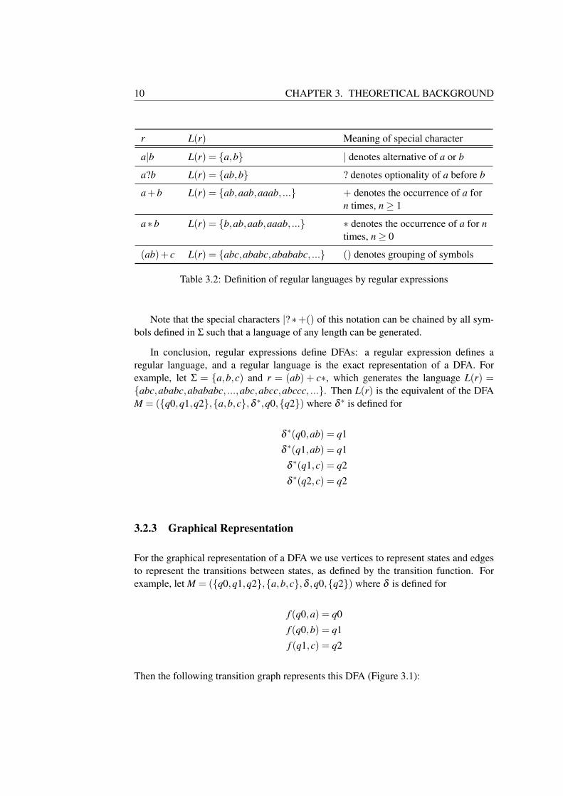
10 CHAPTER 3. THEORETICAL BACKGROUND
r L(r) Meaning of special character
a|b L(r) = {a,b} | denotes alternative of a or b
a?b L(r) = {ab,b} ? denotes optionality of a before b
a+b L(r) = {ab,aab,aaab, ...} + denotes the occurrence of a forn times, n≥ 1
a∗b L(r) = {b,ab,aab,aaab, ...} ∗ denotes the occurrence of a for ntimes, n≥ 0
(ab)+ c L(r) = {abc,ababc,abababc, ...} () denotes grouping of symbols
Table 3.2: Definition of regular languages by regular expressions
Note that the special characters |?∗+() of this notation can be chained by all sym-bols defined in Σ such that a language of any length can be generated.
In conclusion, regular expressions define DFAs: a regular expression defines aregular language, and a regular language is the exact representation of a DFA. Forexample, let Σ = {a,b,c) and r = (ab) + c∗, which generates the language L(r) ={abc,ababc,abababc, ...,abc,abcc,abccc, ...}. Then L(r) is the equivalent of the DFAM = ({q0,q1,q2},{a,b,c},δ ∗,q0,{q2}) where δ ∗ is defined for
δ∗(q0,ab) = q1
δ∗(q1,ab) = q1
δ∗(q1,c) = q2
δ∗(q2,c) = q2
3.2.3 Graphical Representation
For the graphical representation of a DFA we use vertices to represent states and edgesto represent the transitions between states, as defined by the transition function. Forexample, let M = ({q0,q1,q2},{a,b,c},δ ,q0,{q2}) where δ is defined for
f (q0,a) = q0
f (q0,b) = q1
f (q1,c) = q2
Then the following transition graph represents this DFA (Figure 3.1):

3.3. STOCHASTIC STATE ESTIMATION 11
q0
a
q1b
q2c
Figure 3.1: A graphical representation of a DFA as a transition graph.
3.3 Stochastic State Estimation
This section reviews the definition and mathematical concepts of discrete-time stochas-tic systems. In particular, we review the Kalman Filter as a means to minimize theestimated error in a prediction of the future system state. Stochastic state estimationis relevant to the people counting system in order to improve the counting accuracy ofmultiple sensors, as stated in Problem 9. Section 5.5 makes use of the material presentedhere.
3.3.1 Discrete-time Stochastic System
The people counting system presented in this thesis can be seen as a discrete-timestochastic system [15], defined in its general form as
xk+1 = f (xk,uk,k)+wk (3.3.1)
yk = g(xk,uk,k)+ vk (3.3.2)
where matrix xk denotes the state of the system at discrete-time instance k, which in ourcase consists of the true “in” and “out” or “occupancy” scalar values. Matrix yk denotesthe measured state at discrete time k, consisting of the measured “in” and “out” counts(and possibly other information that is of relevance and can be measured). Functionf (·) denotes the state transition function describing the process transition of state xkto state xk+1, using input (control) values uk. Function g(·) relates the state xk to themeasurement yk. wk,vk represent the process and measurement noises, respectively.
In words, given the linear or non-linear functions f (·) and g(·), stochastic stateestimation attempts to predict the future state of a system. For the linear case the abovestate equations are transformed into the following equations:
xk+1 = Akxk +Bkuk +wk (3.3.3)
yk = Hkxk + vt (3.3.4)
where A is the state transition matrix, B is the input transition matrix, and H is themeasurement matrix which relates the current state xk to the measurement yk. Note thatall variables in these equations are matrices.
12 CHAPTER 3. THEORETICAL BACKGROUND
3.3.2 The Kalman Filter
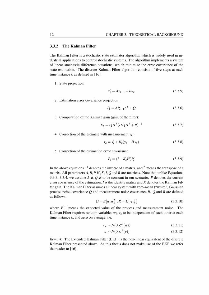
The Kalman Filter is a stochastic state estimator algorithm which is widely used in in-dustrial applications to control stochastic systems. The algorithm implements a systemof linear stochastic difference equations, which minimize the error covariance of thestate estimation. The discrete Kalman Filter algorithm consists of five steps at eachtime instance k as defined in [16]:
1. State projection:
x′k = Axk−1 +Buk (3.3.5)
2. Estimation error covariance projection:
P′k = APk−1AT +Q (3.3.6)
3. Computation of the Kalman gain (gain of the filter):
Kk = P′kHT (HP′kHT +R)−1 (3.3.7)
4. Correction of the estimate with measurement yk :
xk = x′k +Kk(yk−Hxk) (3.3.8)
5. Correction of the estimation error covariance:
Pk = (I−KkH)P′k (3.3.9)
In the above equations −1 denotes the inverse of a matrix, and T means the transpose of amatrix. All parameters A,B,P,H,K, I,Qand R are matrices. Note that unlike Equations3.3.3, 3.3.4, we assume A,B,Q,R to be constant in our scenario. P denotes the currenterror covariance of the estimation, I is the identity matrix and K denotes the Kalman Fil-ter gain. The Kalman Filter assumes a linear system with zero-mean (“white”) Gaussianprocess noise covariance Q and measurement noise covariance R. Q and R are definedas follows:
Q = E[wkwTk ], R = E[vkvT
k ] (3.3.10)
where E[·] means the expected value of the process and measurement noise. TheKalman Filter requires random variables wk,vk to be independent of each other at eachtime instance k, and zero on average, i.e.
wk ∼ N(0,σ2(w)) (3.3.11)
vk ∼ N(0,σ2(v)) (3.3.12)
Remark. The Extended Kalman Filter (EKF) is the non-linear equivalent of the discreteKalman Filter presented above. As this thesis does not make use of the EKF we referthe reader to [16].
CHAPTER 4
People Counting Algorithm for PIRSensors
The focus of this chapter is to analyse the signals by PIR sensors, and to develop analgorithm for people counting. The chapter is organized as follows. To solve Problem 3,we start by analysing the signal patterns of PIR sensors, in particular focusing on thoseaspects relevant to the people counting problem. Algorithms are developed step-by-step, taking into account the insights gained in the process. All algorithms are formallyspecified and described in pseudo-code.
4.1 PIR Sensor Signal Basics
Typical commercially sold PIR sensors emit a binary signal, where a HIGH (binary 1)signal indicates no movement, and a LOW (binary 0) signal indicates the detection ofmovement by the sensor. For our application this information is of little value, as weneed to detect the direction of the movement. Therefore we use PIR sensors providedby Hygrosens, which in addition to the digital signal also provide an analogue output(details see Section 8.2).
PIR sensors are built from two infrared segments, arranged along a horizontal split.The sensor’s analogue signal equals the difference of the infrared radiation received oneach side of the horizontal split, which allows to detect on where in the sensor’s fieldof view a movement originated. Figure 4.1 illustrates the unfiltered analogue signalemitted from the sensor in the event of a single person passing from left to right andback again. The signal as shown was sampled at 50Hz. The pattern reflects the IRradiation, as seen by the sensor, for a single person moving from left to right (range3000− 4000ms), and right to left (range 6000− 7500ms). The continuous signal isinterpolated for readability.
As is easily visible from the figure the signal pattern has several different compo-nents:
1. Signal amplitude. The signal amplitude is a function of the distance of the sensed

14 CHAPTER 4. PEOPLE COUNTING ALGORITHM FOR PIR SENSORS
Figure 4.1: Unfiltered PIR sensor analogue output for a single person traversing fromleft to right and back again. The midpoint of the signal indicates no movement, whereassignal peaks above and below the midpoint refer to maximum incident IR radiation tothe respective side of the PIR sensor.
object passing in front of the sensor. In general, the closer the object to the sensor,the higher the amplitude [17], although the speed of the passing object may alsoinfluence the amplitude [8].
2. Signal frequency. The signal frequency is an indication of the speed of the passingobject. According to the vendor documentation, the signal frequency for our PIRsensors has a bandwidth from 0.2Hz to 10Hz.
3. The phase of the signal (as visible in the time-domain). The phase is an indicationof the side of the sensor where a movement was detected.
The direction of movement can be detected by analysing the phase of the signal. Wesimply approximate this information by using the fact that the PIR sensors output asignal at ≈ VCC/2 while no movement is detected, and the side S of the movement isgiven by
S =
le f t ifs≥VCC/2+ vright ifs≤VCC/2− vsilent otherwise
(4.1.1)
where s indicates the signal’s amplitude and v is a noise threshold above and below VCC2
[5]. Based on our experiments a threshold of v ∼ 260mV works best. Note that sides

4.1. PIR SENSOR SIGNAL BASICS 15
right, left are relative to the mounting direction and can in practice be exchanged foreach other.
The PIR sensors used in the prototype cover a detection range of r = 12m at ahorizontal angle of ±50°. Consider Figure 4.2: assuming the typical installation sce-nario will use sensors ceiling- or side-mounted in entrance doorways of maximumheight/width of 2.5m, we can estimate the distance in relation to the sensor’s rangeas follows. Let the maximal distance dmax =
(2.5−h)sin(180−90−50) , 0.5 ≤ h < 2.5 → 0.02 ≤
dmax < 3.2m, where h is the person height. Then the maximum fraction r′ of the sen-sor’s range covered by our application will be r′ = dmax
r ≤13 r. Even though the sensor’s
amplitude is not strictly linear to the distance [18], we consider the sampled signal forany movement will be in the range vadc = 80 < d(1− r′) · 2adcw
2 e ≤2adcw
2 = 512, whereadcw = 10 is the precision of the ADC in bits and vadc = dadcw · v
VCCe is the signal noiseconverted to its digital representation. Therefore we choose to ignore the variation of thesample signal (due to person height) for the purpose of this discussion. Note we use thesignal noise v as a lower bound because the sensors report the difference of the incidentIR radiation between the two IR elements rather than an absolute value for each. Thus,in practice, the signal can be well below the theoretical minimum of d2
3 ·2adcw
2 e= 342 atr′ = 1
3 , however, we consider all signals above the noise level as by Equation 4.1.1.
We will later show that the signal frequency is of marginal importance in our appli-cation since we are only interested in the fact that a passage has occurred, but not in howfast this happened. However, the frequency bandwidth is of relevance to the samplingfrequency of the sensor as it provides a natural bound in terms of the Nyquist frequency.Hence, the sample frequency shall be at least fmax · 2 ≥ 20Hz where 0.2 ≤ f ≤ 10 isthe PIR sensor’s frequency spectrum. Based on our experiments f = 50Hz yields asufficient resolution and sample spacing in the time domain.
Figure 4.2: Assumed maximal distances and minimal person height. The distancesallow to approximate the sensor signal strength to fall within a limited range despitepeople height. That is, we can ignore variation in the signal due to person height. Notethat this may no longer be true if the door height exceeds the given limits.

16 CHAPTER 4. PEOPLE COUNTING ALGORITHM FOR PIR SENSORS
4.2 Deriving a People Count
Consider again Figure 4.1 depicting the PIR sensor output for one person, passing oncein each direction. We can see two distinct peaks at the lowest and highest points of theamplitude range. The peaks signify the moment of strongest incident IR radiation onthe left or right side of the sensor’s field-of-view, respectively. The passages from leftto right and vice versa are clearly visible: for each passage, the signal peaks on the fromside, next on the to (opposite) side. From this analysis, the people count seems to equalthe number of transitions t( f rom, to). Unfortunately, this rule is not always applicablein the case of multiple people passing in a queue and with little distance, as will bediscussed next.
Consider Figure 4.3. It depicts the signal output for four people passing by the sen-sor from left to right. Unlike the single-person example, no specific left/right passagesare visible, except for the first. Further, and unlike the single-person passage, the sig-nal does not provide clues to separate one person from the other. Clearly, counting thetransitions as in the first example will produce false positives.
Looking further, the signal contains several high frequency ranges. The signal fre-quency corresponds to the angular speed of each person passing by. Since we are in-terested in the number of people we might simply count the number of distinct high-frequency areas. However, this turns out to be impractical as we can see in Figure 4.4:applying a high-pass filter correctly yields the high-frequency areas, but these areasare too close to each other to count the number of passers-by. Therefore we concludethat isolating the high-frequency areas of a sampled signal is not practical to solve ourproblem.
Let us consider again Figure 4.3, but this time focus on low-frequency peaks. Fourpeaks are clearly visible in the amplitude range of 0 ≤ s ≤ 200 and two peaks in therange 900≤ s≤ 1023: each of these peaks is a result of one person passing the sensor ata distance close enough to yield an amplitude above the silent threshold level. The fourpeaks exactly reflect the number of people arriving at the passage’s opposite side. Recallthat samples are spaced 1
50 s = 20ms apart, and consider the distance between thesepeaks: each person takes between 0.5s and 1s to pass. This is reasonable considering thesensor’s range we are interested in, the installation height, a walking speed of ∼ 5km/h,and an average person height of 1.7m.
In conclusion, to count the number of people passing in a queue at short distance,the sensor signal must be interpreted from the first detected passage, coming from asilent state. The first change in amplitude indicates the from direction, and the imme-diate subsequent amplitude peak on the opposite side indicates the to direction. Anysubsequent low-frequency peak indicates one more person passing in line. The countingsequence completes with a silent phase.

4.3. BASIC ALGORITHM 17
Figure 4.3: Signal pattern for four people in a row traversing from right to left.
4.3 Basic Algorithm
As shown in the last section the raw sensor signal allows for a visual analysis by count-ing the number of low-frequency peaks on one side of the sensor, after detecting thefirst passage. The COUNT algorithm (Algorithm 1) applies this insight. Assume thesignal has been analysed for low-frequency peaks outside the silent amplitude range.The algorithm works in two stages:
1. Identify a first passage left/right or right/left. This becomes the direction of move-ment.
2. Count the number of transitions c = (direction) by counting the peaks on the toside of the sensor.
While this basic algorithm works correctly for the previously identified patterns of PIRsignals, it is not sufficient for practical applications due to several reasons:
1. Distortions and noise in the signal are not accounted for and will lead to falsepeak identification and thus invalid count values. An example is given in Fig-ure 4.5, where a single person has passed the sensor yet yielding two peaks onthe to side of the amplitude range. Such a pattern may be caused by a rela-tively slow moving person, where the sensor indicates IR radiation at differentangles. This kind of distortion can be eliminated by filtering the signal to in-clude only the relatively low-frequency components indicating amplitude shifts.

18 CHAPTER 4. PEOPLE COUNTING ALGORITHM FOR PIR SENSORS
Figure 4.4: Signal pattern for four people in a row traversing from right to left, withhigh-pass filter applied (filtered signal adjusted for visual overlay).
2. The first transition from an identified from peak to an adjoint to peak must happenwithin a limited amount of time, that is below time distance t ≤ tdmax. If too muchtime passes between these two peaks the algorithm should ignore the previouspeak and assume it has started from a silent position. Applying this rule simplifiesthe handling of fast changes in the direction of movement, such as when a groupof people passes by the sensor in one direction first, followed by another groupthat walks in the opposite direction.
3. Multiple peaks in short distance such as in Figure 4.5 may cause false counts. Tolimit the number of counts within a sequence, a minimal time distance t ≥ tdmin
between peaks must be observed.
4. To distinguish people standing/waiting in the sensor’s field of view, vs. someoneactually passing it, an absolute distance of peaks in terms of the signal’s amplitude|s(t)− s(t−1)| ≥ amin should be observed (Figure 4.6).
The following sections discuss improvements to the COUNT algorithm to alleviate theseproblems. In particular, Section 4.4 introduces signal filtering to reduce distortionsand noise; Section 4.5 provides a peak detection algorithm; Section 4.6 describes theimplementation of the algorithm as a finite state machine, and Section 4.7 extends thisidea by using regular expressions to enable run-time adjustments of the state machine.
4.4. SIGNAL FILTER 19
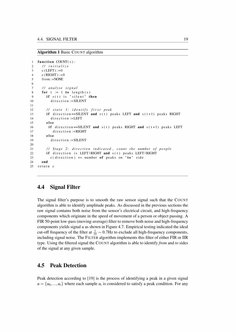
Algorithm 1 Basic COUNT algorithm
1 f u n c t i o n COUNT( s ) :2 / / i n i t i a l i z e3 c ( LEFT ) :=04 c (RIGHT) :=05 from :=NONE67 / / a n a l y s e s i g n a l8 f o r t := 1 to l e n g t h ( s )9 i f s ( t ) i s " s i l e n t " then
10 d i r e c t i o n := SILENT1112 / / s t a t e 1 : i d e n t i f y f i r s t peak13 i f d i r e c t i o n ==SILENT and s ( t ) peaks LEFT and s ( t +1) peaks RIGHT14 d i r e c t i o n :=LEFT15 e l s e16 i f d i r e c t i o n ==SILENT and s ( t ) peaks RIGHT and s ( t +1) peaks LEFT17 d i r e c t i o n :=RIGHT18 e l s e19 d i r e c t i o n := SILENT2021 / / S t a g e 2 : d i r e c t i o n i n d i c a t e d , c o u n t t h e number o f p e o p l e22 i f d i r e c t i o n i s LEFT | RIGHT and s ( t ) peaks LEFT | RIGHT23 c ( d i r e c t i o n ) += number of peaks on " to " s i d e24 end25 r e t u r n c
4.4 Signal Filter
The signal filter’s purpose is to smooth the raw sensor signal such that the COUNT
algorithm is able to identify amplitude peaks. As discussed in the previous sections theraw signal contains both noise from the sensor’s electrical circuit, and high-frequencycomponents which originate in the speed of movement of a person or object passing. AFIR 50-point low-pass (moving-average) filter to remove both noise and high-frequencycomponents yields signal u as shown in Figure 4.7. Empirical testing indicated the idealcut-off frequency of the filter at 1
35 ∼ 0.7Hz to exclude all high-frequency components,including signal noise. The FILTER algorithm implements this filter of either FIR or IIRtype. Using the filtered signal the COUNT algorithm is able to identify from and to sidesof the signal at any given sample.
4.5 Peak Detection
Peak detection according to [19] is the process of identifying a peak in a given signalu = {u0, ...,ut} where each sample ut is considered to satisfy a peak condition. For any

20 CHAPTER 4. PEOPLE COUNTING ALGORITHM FOR PIR SENSORS
Figure 4.5: PIR signal with multiple peaks for a single person traversing in one di-rection. The pattern yields two peaks, and thus causes the basic COUNT algorithm(Algorithm 1) to count two people. This can be alleviated by applying a filter to thesensor signal, such that there is only one peak.
given sample ut we derive the standard deviation
σt =
√1
2sw
t+sw
∑i=t−sw
(u′i−m) (4.5.1)
of all samples u′ = {us : t− sw < s < t+ sw}, where sw is the number of samples beforeand after ut (i.e. window width), m is the mean of all samples in u′, that is
m =1
2sw+1
2sw+1
∑i=1
u′i (4.5.2)
A peak is identified for all samples ut whose variance vt = |ut −m| ≥ σ . Statistically,the idea is to identify all samples which exceed the threshold of one standard deviationof their ±sw neighbours. All peaks within the signal are identified accordingly as P ={pt : ut ∈ u, vt ≥ σ}. The PEAK algorithm (Algorithm 2) is implemented accordingly.Note that
p[t] =
{u[t] if peak identified⊥ otherwise
, ⊥denotes no peak. (4.5.3)
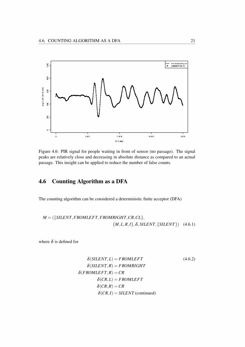
4.6. COUNTING ALGORITHM AS A DFA 21
Figure 4.6: PIR signal for people waiting in front of sensor (no passage). The signalpeaks are relatively close and decreasing in absolute distance as compared to an actualpassage. This insight can be applied to reduce the number of false counts.
4.6 Counting Algorithm as a DFA
The counting algorithm can be considered a deterministic finite acceptor (DFA)
M = ({SILENT,FROMLEFT,FROMRIGHT,CR,CL},{M,L,R, I},δ ,SILENT,{SILENT}) (4.6.1)
where δ is defined for
δ (SILENT,L) = FROMLEFT (4.6.2)
δ (SILENT,R) = FROMRIGHT
δ (FROMLEFT,R) =CR
δ (CR,L) = FROMLEFT
δ (CR,R) =CR
δ (CR, I) = SILENT (continued)

22 CHAPTER 4. PEOPLE COUNTING ALGORITHM FOR PIR SENSORS
Figure 4.7: Filtered signal using a FIR 50-point moving average filter. Note both theinput signal and the filter output have been interpolated to form continuous lines forvisual emphasis of the differences.
δ (FROMRIGHT,L) =CL
δ (CL,R) = FROMRIGHT
δ (CL,L) =CL
δ (CL, I) = SILENT
δ (FROMLEFT, I) = SILENT
δ (FROMRIGHT, I) = SILENT
Using the output of the PEAK algorithm (Algorithm 2), COUNT assigns each peak pt ∈Pa character ct ∈ Σ according to the rules of Equation 4.1.1, where t is the discrete time.The symbol I (“ignore”) is used to denote a peak pt which has too large a time distanceto the previous peak, that is for its peak time pti it holds that pti− pti−1 > tdmax. Twoassociated counters cright ,cle f t keep track of the number of transitions to states CR andCL, respectively.
In words, SILENT is the initial state and a state transition to SILENT occurs uponprocessing a sample whose time distance to the previous peak is larger than the thresh-old, tdmax. A state transition to FROMLEFT occurs upon detecting a peak on the leftof the signal amplitude range, and a state transition to CR occurs subsequently as manytimes as required, until a transition to SILENT is raised. The same applies respectivelyto the states FROMRIGHT and CL.
4.6. COUNTING ALGORITHM AS A DFA 23
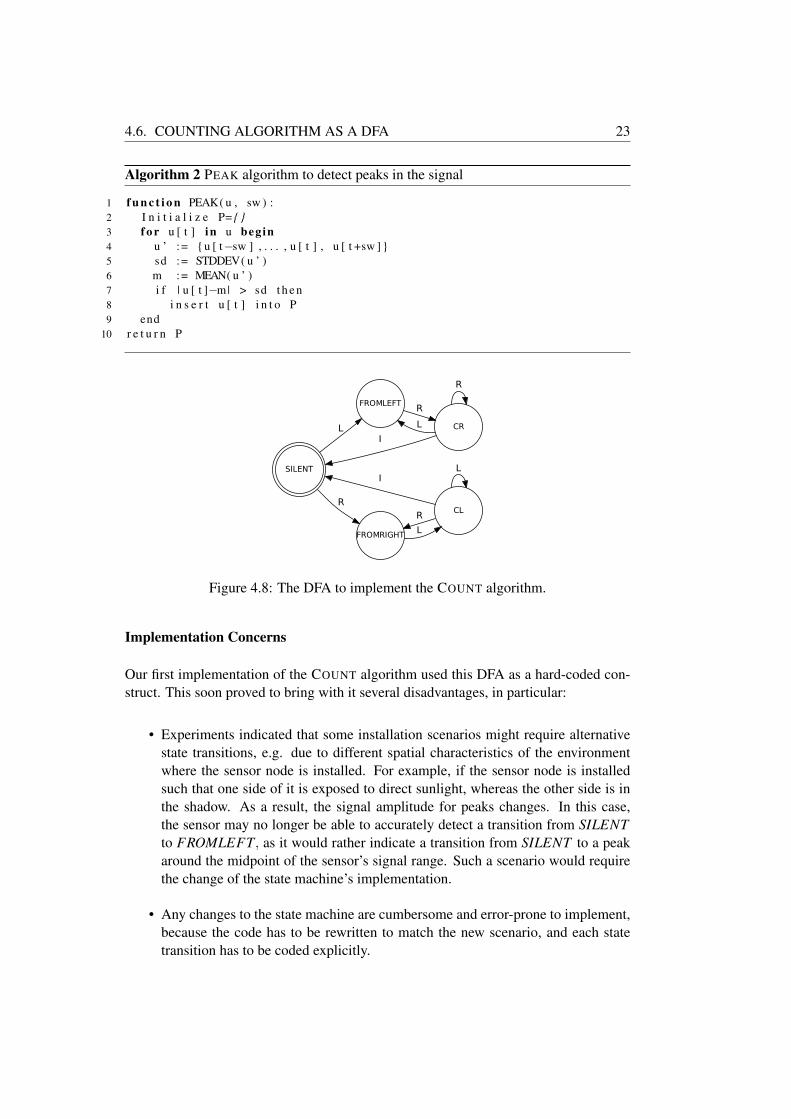
Algorithm 2 PEAK algorithm to detect peaks in the signal
1 f u n c t i o n PEAK( u , sw ) :2 I n i t i a l i z e P={ }3 f o r u [ t ] in u begin4 u ’ := {u [ t−sw ] , . . . , u [ t ] , u [ t +sw ] }5 sd := STDDEV( u ’ )6 m := MEAN( u ’ )7 i f | u [ t ]−m| > sd t h e n8 i n s e r t u [ t ] i n t o P9 end
10 r e t u r n P
SILENT
FROMLEFT
L
FROMRIGHT
R
CR
R
I
L
R
CL
L
I
R
L
Figure 4.8: The DFA to implement the COUNT algorithm.
Implementation Concerns
Our first implementation of the COUNT algorithm used this DFA as a hard-coded con-struct. This soon proved to bring with it several disadvantages, in particular:
• Experiments indicated that some installation scenarios might require alternativestate transitions, e.g. due to different spatial characteristics of the environmentwhere the sensor node is installed. For example, if the sensor node is installedsuch that one side of it is exposed to direct sunlight, whereas the other side is inthe shadow. As a result, the signal amplitude for peaks changes. In this case,the sensor may no longer be able to accurately detect a transition from SILENTto FROMLEFT, as it would rather indicate a transition from SILENT to a peakaround the midpoint of the sensor’s signal range. Such a scenario would requirethe change of the state machine’s implementation.
• Any changes to the state machine are cumbersome and error-prone to implement,because the code has to be rewritten to match the new scenario, and each statetransition has to be coded explicitly.
24 CHAPTER 4. PEOPLE COUNTING ALGORITHM FOR PIR SENSORS
As an alternative the next section considers an implementation where the FSM is im-plemented by means of a regular expression.
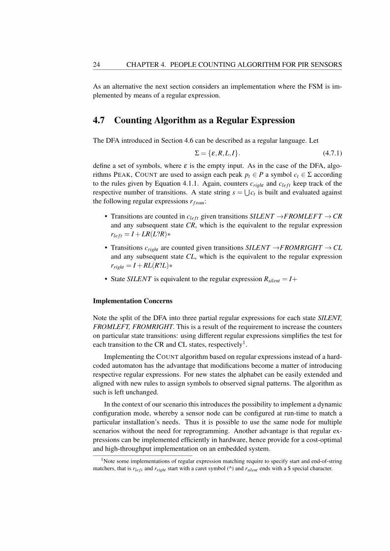
4.7 Counting Algorithm as a Regular Expression
The DFA introduced in Section 4.6 can be described as a regular language. Let
Σ = {ε,R,L, I}. (4.7.1)
define a set of symbols, where ε is the empty input. As in the case of the DFA, algo-rithms PEAK, COUNT are used to assign each peak pt ∈ P a symbol ct ∈ Σ accordingto the rules given by Equation 4.1.1. Again, counters cright and cle f t keep track of therespective number of transitions. A state string s =
⋃ct is built and evaluated against
the following regular expressions r f rom:
• Transitions are counted in cle f t given transitions SILENT →FROMLEFT →CRand any subsequent state CR, which is the equivalent to the regular expressionrle f t = I +LR(L?R)∗
• Transitions cright are counted given transitions SILENT →FROMRIGHT →CLand any subsequent state CL, which is the equivalent to the regular expressionrright = I +RL(R?L)∗
• State SILENT is equivalent to the regular expression Rsilent = I+
Implementation Concerns
Note the split of the DFA into three partial regular expressions for each state SILENT,FROMLEFT, FROMRIGHT. This is a result of the requirement to increase the counterson particular state transitions: using different regular expressions simplifies the test foreach transition to the CR and CL states, respectively1.
Implementing the COUNT algorithm based on regular expressions instead of a hard-coded automaton has the advantage that modifications become a matter of introducingrespective regular expressions. For new states the alphabet can be easily extended andaligned with new rules to assign symbols to observed signal patterns. The algorithm assuch is left unchanged.
In the context of our scenario this introduces the possibility to implement a dynamicconfiguration mode, whereby a sensor node can be configured at run-time to match aparticular installation’s needs. Thus it is possible to use the same node for multiplescenarios without the need for reprogramming. Another advantage is that regular ex-pressions can be implemented efficiently in hardware, hence provide for a cost-optimaland high-throughput implementation on an embedded system.
1Note some implementations of regular expression matching require to specify start and end-of-stringmatchers, that is rle f t and rright start with a caret symbol (^) and rsilent ends with a $ special character.

4.8. FINALIZED COUNT ALGORITHM 25
4.8 Finalized COUNT Algorithm
Taking into account the previous sections, we can now specify the finalized COUNT
algorithm (Algorithm 3) as follows. The algorithm uses four stages:
1. Apply a low-pass filter to the input signal to reduce signal noise and extract theinformation indicating an object passing by the sensor.
2. Identify the signal peaks pt as those samples that identify either the beginning ofa traversal, or a subsequent peak on the opposite side.
3. Assign each peak a character of the regular language alphabet Σ of the countingstate machine, and build a state string s =
⋃ct .
4. Use the regular expressions Rright , Rle f t , Rsilent to identify patterns in the statestring. On a match, count the respective traversal (or ignore the peak in the caseof a SILENT state).
Algorithm 3 The finalized COUNT algorithm (part 1)
1 FUNCTION COUNT( s ) :2 # i n i t i a l i z e3 c ( l e f t , r i g h t ) = 04 c ( r i g h t , l e f t ) = 05 pt_max = 100 # max# samples between two peaks6 s = " " # s t a t e s t r i n g7 s i = 0 # s t a t e s t r i n g i n d e x8 MIDPOINT = ADC(VCC/ 2 ) # d e f i n e t h e ADC m i d p o i n t9 MIDTHRES = 80 # +/− 80 (2 x80 <= 169)
10 ABSTHRES = 150 # minimal a m p l i t u d e d i s t a n c e11 MAXDIST = 100 # maximal t ime d i s t a n c e12 MATCH_LEFT = / I +LR( L?R) * /13 MATCH_RIGHT = / I +RL(R?L ) * /14 MATCH_SILENT = / I +$ / # on ly match a t end of s t r i n g15 # S t a g e s 1 ,216 y = FILTER ( s )17 p = PEAK( y )18 # S t a g e 3 ,4 a n a l y s e s i g n a l19 f o r ( each peak t in p )20 i f p t [ t ] − p t [ t −1] <= MAXDIST and ( p t−p t [ t −1] > ABSTHRES) then21 # S t a g e 322 s i = s i + 123 i f p [ t ] − MIDPOINT > 0 then s [ s i ] = "L"24 i f p [ t ] − MIDPOINT < 0 then s [ s i ] = "R"25 i f abs ( p [ t ] − MIDPOINT) <= MIDTHRES then s [ s i ] = "M"26 ( c o n t i n u e d )
26 CHAPTER 4. PEOPLE COUNTING ALGORITHM FOR PIR SENSORS
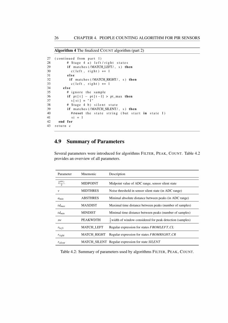
Algorithm 4 The finalized COUNT algorithm (part 2)
27 ( c o n t i n u e d from p a r t 1 )28 # S t a g e 4 a ) l e f t / r i g h t s t a t e s29 i f matches ( / MATCH_LEFT/ , s ) then30 c ( l e f t , r i g h t ) += 131 e l s e32 i f matches ( / MATCH_RIGHT/ , s ) then33 c ( l e f t , r i g h t ) += 134 e l s e35 # i g n o r e t h e sample36 i f p t [ t ] − p t [ t −1] > pt_max then37 s [ s i ] = " I "38 # S t a g e 4 b ) s i l e n t s t a t e39 i f matches ( / MATCH_SILENT / , s ) then40 # r e s e t t h e s t a t e s t r i n g ( b u t s t a r t in s t a t e I )41 s i = 142 end f o r43 r e t u r n c
4.9 Summary of Parameters
Several parameters were introduced for algorithms FILTER, PEAK, COUNT. Table 4.2provides an overview of all parameters.
Parameter Mnemonic Description
2ADCw
2 MIDPOINT Midpoint value of ADC range, sensor silent state
v MIDTHRES Noise threshold in sensor silent state (in ADC range)
amin ABSTHRES Minimal absolute distance between peaks (in ADC range)
tdmax MAXDIST Maximal time distance between peaks (number of samples)
tdmin MINDIST Minimal time distance between peaks (number of samples)
sw PEAKWDTH 12 width of window considered for peak detection (samples)
rle f t MATCH_LEFT Regular expression for states FROMLEFT,CL
rright MATCH_RIGHT Regular expression for states FROMRIGHT,CR
rsilent MATCH_SILENT Regular expression for state SILENT
Table 4.2: Summary of parameters used by algorithms FILTER, PEAK, COUNT.
CHAPTER 5
Implementation
In this chapter we discuss the implementation of the algorithms in the C-language inorder to program a sensor node, an embedded system with limited computing and mem-ory resources. An overview of the validation framework is presented, which enables thecomparison and validation of the performance of algorithms as implemented in the Cand R programming languages.
In solving Problem 6 and Problem 7 the technical aspects of a monitoring applica-tion and a data collection server are summarised. To conclude, we present a solutionsketch to the space occupancy estimation Problem 9. The Appendix lists reference in-formation and technical details.
5.1 System Overview
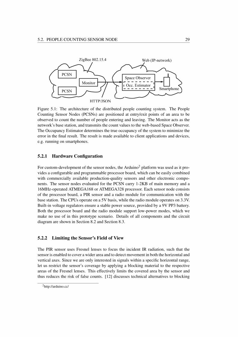
Figure 5.1 depicts the architecture of the system. The system consists of the followingelements.
People Counting Sensor Nodes A People Counting Sensor Node (PCSN) uses a double-element passive infrared sensor (PIR) connected to a microcontroller. The micro-controller continuously analyses the PIR’s output signal to detect and count thenumber of people passing it. A successful pass is a traversal from one side of thePIR’s field of view (FOV) to the other. Each pass increases the count in either theleft or the right direction as seen from the PCSN’s installation point. The PCSNperiodically transmits the determined number of passes to a base station in theSensor Network.
Sensor Network The Wireless Sensor Network (WSN) is a hierarchical or mesh-styletopology of sensor nodes, in particular PCSNs. Each PCSN is connected to a basestation via the ZigBee network protocol1. The protocol provides the infrastructurefor node connection, routing and data collection. The WSN’s base station has a
1Specified by the ZigBee Alliance (http://www.zigbee.org) and based on the IEEE 802.15.4 standardfor low-rate wireless personal area networks.
28 CHAPTER 5. IMPLEMENTATION
double role: First, it acts as the sink node in the sensor network. Second, it isthe gateway to the web-based space observer. It collects the count data from allPCSNs and forwards these to the web-based Space Observer.
Space Model and Monitor The Space Model defines the physical distribution of PC-SNs to cover a specific area for which to count people and derive the occupancylevel. The Monitor is an application installed on the WSN’s base station to col-lect all count data of associated PCSNs, and to forward these observations to theweb-based space observer.
Web-based Space Observer The Space Observer allows for the definition of multiple(spatial) spaces. For each space the server records the “in” and “out” countsand calculates the current occupancy of each defined space by use of the ProcessEstimator. The occupancy is measured as an absolute number and related as apercentage to the known capacity of an area.
Occupancy Estimator The space model serves as the basis for the Occupancy Esti-mator to estimate the occupancy of each space. Because the PCSNs’ count dataare diluted by measurement noise (false counts), the occupancy of a space cannotsimply be calculated. Instead, a stochastic process is assumed, and the occupationis estimated by the use of a stochastic process estimator, such as the Kalman Filter(Section 5.5). The space model defines a space as some spatial area that is ob-served by sensors for the number of people entering (“in”) and leaving (“out”) thearea. The stochastic process assumes noisy measurements of in and out counts(the process measurement), and derives an estimation of the actual occupation(process state) for each space. This data can then be used to display an occupa-tion of spaces to the user e.g. via smartphone user interface.
Smartphone User Interface The Smartphone User Interface is supposed to signifysome end-user device capable of querying the web-based space observer. It islisted here for completeness but is not realized as part of this thesis.
Validation Framework The validation framework provides the means to analyse thePCSN’s performance off-line. That is, the validation framework provides algo-rithms implemented in the R-language and allows to analyse their respective C-language implementation output based on previously recorded data.
5.2 People Counting Sensor Node
For programming the prototype sensor nodes, the algorithms were transformed fromtheir R language implementation into the C language. This chapter first introduces thehardware setup, and next outlines the changes applied due to the specific constraints ofthe sensor node as an embedded system.
5.2. PEOPLE COUNTING SENSOR NODE 29
PCSN
PCSN
Monitor
ZigBee 802.15.4
Space Observer
Occ. Estimator
Web (IP-network)
HTTP/JSON
Smartphone
Figure 5.1: The architecture of the distributed people counting system. The PeopleCounting Sensor Nodes (PCSNs) are positioned at entry/exit points of an area to beobserved to count the number of people entering and leaving. The Monitor acts as thenetwork’s base station, and transmits the count values to the web-based Space Observer.The Occupancy Estimator determines the true occupancy of the system to minimize theerror in the final result. The result is made available to client applications and devices,e.g. running on smartphones.
5.2.1 Hardware Configuration
For custom-development of the sensor nodes, the Arduino2 platform was used as it pro-vides a configurable and programmable processor board, which can be easily combinedwith commercially available production-quality sensors and other electronic compo-nents. The sensor nodes evaluated for the PCSN carry 1-2KB of main memory and a16MHz-operated ATMEGA168 or ATMEGA328 processor. Each sensor node consistsof the processor board, a PIR sensor and a radio module for communication with thebase station. The CPUs operate on a 5V basis, while the radio module operates on 3.3V.Built-in voltage regulators ensure a stable power source, provided by a 9V PP3 battery.Both the processor board and the radio module support low-power modes, which wemake no use of in this prototype scenario. Details of all components and the circuitdiagram are shown in Section 8.2 and Section 8.3.
5.2.2 Limiting the Sensor’s Field of View
The PIR sensor uses Fresnel lenses to focus the incident IR radiation, such that thesensor is enabled to cover a wider area and to detect movement in both the horizontal andvertical axes. Since we are only interested in signals within a specific horizontal range,let us restrict the sensor’s coverage by applying a blocking material to the respectiveareas of the Fresnel lenses. This effectively limits the covered area by the sensor andthus reduces the risk of false counts. [12] discusses technical alternatives to blocking
2http://arduino.cc/

30 CHAPTER 5. IMPLEMENTATION
IR radiation such as constructing a blind cover. For the purpose of our experiments wehave found white adhesive office-supply gum to be sufficient.
5.2.3 Need for Iterative Algorithms
The algorithms considered so far operate on the full length of a given signal. On thesensor node this is unrealistic since the available memory and CPU processing capacityare limited. It is essential that the algorithms FILTER, COUNT, PEAK are modified, suchthat they process one sample at a time and only use a small amount of memory in doingso.
Processing Scheme The algorithms for the sensor node follow an iterative processingscheme, such that the signal u[k] is transformed into output c[k] as
c[k] =COUNT (PEAK(FILT ER(u[k]))) (5.2.1)
where u[k] denotes the sample at time k as given by the ATMEGA328’s internalanalogue-digital converter (ADC), and FILTER, PEAK, COUNT are the modified low-pass filter, peak detection and counter algorithms, respectively. c[k] is a vector to containthe transition counts, c[k] = [cle f t ,cright ]. The ADC converts the analogue input signalprovided by the sensor at a rate of 50Hz using a timer interrupt. Upon completion ofthe conversion, the sampled signal is transferred and processed as defined above.
Ring Buffer for Iterative Algorithms To process the input signal iteratively, FILTER,PEAK, COUNT need to access both the current input sample u[k] and a certain numberof previously calculated (filtered) output samples y[k]. Due to the memory constraintson the sensor node, it is infeasible to hold all calculated output samples in memory.Ring buffers are implemented for the input u, filter output y and peak p vectors. Eachring buffer is a vector of dimension b which denotes the buffer size as the maximumnumber of items stored in the buffer. The ring buffer operates such that the accessedsample index i = k is calculated as the ring buffer’s vector index i′ given by
i′ =
{imodb if i≥ 0b+ i otherwise
, |i| ≤ b (5.2.2)
5.2.4 Iterative FILTER algorithm
A first C-language implementation of the FILTER algorithm using the FIR kernel demon-strated that this implementation is infeasible given the limits of the sensor nodes. Thealgorithm in principle would work sufficiently fast, and does not as such exhaust thememory. For the filter to work, the data structure requires an array of 50+100−1= 149entries in order to store both, the samples and the filter kernel. Each sample takes 4 bytes

5.2. PEOPLE COUNTING SENSOR NODE 31
of memory (of type float). However, the sensor node also stores the count vector, debugstrings and requires other temporary storage. Thus, the total heap memory requirementin excess of 1KB memory would break the limits of the ATMEGA168-based sensornode, which served as a test board.
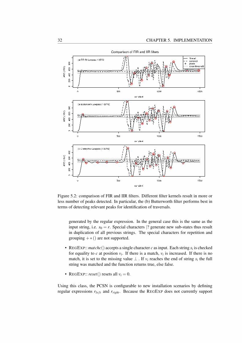
Based on experiments using the R Signal3 package [20], a recursive implementationof an infinite impulse response (IIR) was chosen. Several different filters were consid-ered and compared; Figure 5.2 depicts a comparison of several filters applied to thesame input signal.
The figure depicts in (a) the FIR low-pass filter described in Section 4.4 and the re-sulting output signal. (b) shows the result of a four-pole Butterworth low-pass filter, (c)represents the result of a Chebychev four-pole filter. The peaks shown are those foundby the PEAK algorithm. All filters use the same cut-off frequency ( 1
35 of the Nyquistfrequency f/2, equals 0.71Hz at sampling frequency f = 50Hz). The Chebychev filterhas a band-pass ripple of 1%, which is clearly visible in (c) around samples 0-500, 600-650, and 1250-1500. This ripple is a potential source for the false detection of peaks inthe filtered signal. The Butterworth filter performs best in this respect among all filters(0% ripple), and also matches the result of FIR filter (a) closely.
5.2.4.1 Iterative PEAK and COUNT algorithms
The PEAK and COUNT algorithms are modified such that they accept a single inputsample u[k], process and store the result y[k] into the respective ring buffer. PEAK
accesses FILTER’s output from ring buffer y, and then stores the identified peaks p[k] inring buffer p. COUNT accesses ring buffer p and updates the count values in vector c.Note that vector c is not a ring-buffer as it holds the scalar sum of the transition counts.
5.2.4.2 Iterative Regular Expression
Building the state string s on the PCSN may lead to buffer overflow or overwritingof previous states in the ring buffer. The following approach solves this problem byusing a simplified regular expression evaluator, REGEXP: it accepts single charactersiteratively. Thus, there is no need to buffer s. REGEXP is implemented as a C++ classand works as follows4:
• REGEXP:: make() accepts a regular expression r as an input string. It parses theregular expression and builds an internal representation of the DFA. The internalrepresentation equals the language L(r), i.e. the set S = {s0, ...,sn} of all strings
3A MATLAB-equivalent implementation of digital signal processing functions4REGEXP was implemented as a proof of concept and is not optimized for space nor time complexity.
For example, matchc() has a worst-case time complexity O(n2) where n is the number of states in the DFA.An improved version using a more efficient internal encoding could perform significantly better, e.g. usinga binary tree to store and access states, reducing matchc()’s worst-time complexity to O(n logn).
32 CHAPTER 5. IMPLEMENTATION
Figure 5.2: comparison of FIR and IIR filters. Different filter kernels result in more orless number of peaks detected. In particular, the (b) Butterworth filter performs best interms of detecting relevant peaks for identification of traversals.
generated by the regular expression. In the general case this is the same as theinput string, i.e. s0 = r. Special characters |? generate new sub-states thus resultin duplication of all previous strings. The special characters for repetition andgrouping +∗ () are not supported.
• REGEXP:: matchc() accepts a single character c as input. Each string si is checkedfor equality to c at position vi. If there is a match, vi is increased. If there is nomatch, it is set to the missing value ⊥ . If vi reaches the end of string si the fullstring was matched and the function returns true, else false.
• REGEXP:: reset() resets all vi = 0.
Using this class, the PCSN is configurable to new installation scenarios by definingregular expressions rle f t and rright . Because the REGEXP does not currently support

5.3. SPACE MODEL, MONITOR AND OBSERVER 33
repetition or grouping, several changes to the C-language implementation of the COUNT
algorithms were necessary:
• The algorithm tracks the states FROMLEFT and FROMRIGHT explicitly.
• The regular expressions are redefined to rle f t = LRL?, rright = RLR?, a match isonly attempted if the time distance pti− pti−1 ≤ tdmax (to compensate for themissing character I in the regular expressions).
• The regular expression Rsilent is replaced by a direct test for the maximal timedistance tdmax.
• Each time a match occurs on either rle f t or rright the respective instance of REG-EXP is reset. This is the equivalent of matching the start of the string the nexttime around.
5.2.5 Operation Modes of the PCSN
The PCSN implements two modes of operation: a LOGGER mode, which is used tosample unfiltered values, and a COUNT ER mode which is used to operate the sensornode as an independent people counter. The LOGGER mode is designed to be usedfor experimental data collection: all sensor values are transmitted to and stored by aPC for subsequent analysis. In this mode, the PCSN does not filter or process thedata in any way. In COUNT ER mode the PCSN only transmits (a) the scalar countvalues cle f t , cright , and (b) string s since the last peak was processed. Note that fordebugging purpose, s is amended by + and − signs to mark transitions to CL and CRstates, respectively.
The PCSN accepts a configuration value SERIAL and RF. The SERIAL configura-tion implies use of the sensor node’s USB port to transmit the data. The RF configura-tion implies use of the ZigBee radio transmission module.
5.3 Space Model, Monitor and Observer
5.3.1 Monitoring Model
The PCSN is designed to be installed such that the PIR sensor’s left/right sides corre-spond to an observed space’s entry/exit directions, respectively. If multiple PCSNs arecombined, a larger spatial area can be observed, and the occupancy of the area can bederived from the total of the count.
Thus, the monitoring model is defined as follows:
Definition 10 (Monitoring Model). A spatial area S of size SA subdivided by N sub-areas Si,0 < i ≤ N of size SA(i) such that SA = ∑SA(i). Each sub-area Si has a pre-determined maximal occupancy (number of passengers), and is monitored by a set of

34 CHAPTER 5. IMPLEMENTATION
PCSNs Ci : {c0, ...,ck}. Each node is positioned to monitor one entry/exit point of therespective sub-area.
By Definition 10, all nodes in a set Ni form a segment of the sensor network witha local root node acting as the base station for this segment. A segment is defined asfollows:
Definition 11 (Monitoring Segment). A set of PCSNs interconnected as a spanning tree,where the root node is said to be the base station. At an appropriate frequency, nodessend their acquired data to the root node. In general, a recursive hierarchy of nodes maybe used to represent segments of segments.
5.3.2 Sensor Monitor (Base Station)
Each base station implements a Sensor Monitor which connects to one or multiple PC-SNs operated in COUNT ER mode. The Sensor Monitor receives count data via a radiolink. A prototype implementation of two PCSNs connected to a base station has beenimplemented as a Java application (SENSMON). For this purpose, both the base sta-tion and the PCSNs are extended by RF modules using the ZigBee 802.15.4 networkingprotocol.
For each PCSN connected, SENSMON displays a visual representation of the countvalues, symbolising in/out counts for an observed area, respectively. Upon receptionof a new count value, SENSMON updates the display accordingly (see screenshot inSubsection 8.5.1).
An extension to SENSMON was added to enable the interfacing with the Data Col-lection Server described in Subsection 5.3.4.
5.3.3 Sensor Network Data Transmission
The ZigBee 802.15.4 protocol supports star, meshed and hierarchical network topolo-gies. Note that the RF modules used for the prototype implementation only support thestar topology, which is sufficient for the purpose of the prototype. Each RF module isassigned a pre-defined node ID. A hardware configuration setting defines the role ofeach RF module in the network (client or controller).
A simple application protocol layer was developed to enable the binary transmissionof arbitrary data structures. It is based on the open-source library xbee-arduino5, whichimplements an application programming interface (API) to the RF modules. The appli-cation protocol layer provides the following functions and a message data structure:
• RFMESSAGE is the message data structure for both, requests and responses. Thestructure contains a 1-byte field for application use, e.g. to indicate the type of
5http://code.google.com/p/xbee-arduino/

5.3. SPACE MODEL, MONITOR AND OBSERVER 35
message exchanged, and a payload field of maximum size RFMESSAGESIZE(defaults to 10 bytes). The payload field can be accessed as an array of bytes, asa string of characters, as a 16-bit integer or an unsigned byte.
• getRequest() to receive a packet from the MAC layer; returns a pointer to theRFMESSAGE structure.
• sendResponse() to send a reply package; uses a RFMESSAGE structure to mar-shal payload data in little endian coding.
If configured for RF transmission, the PCSN invokes the sendResponse() function pe-riodically to transmit the content of the transition count vector c. The periodicity isconfigurable. If a period (default: 1000ms) has elapsed, the transmission is scheduled,immediately following completion of the COUNT algorithm. The sendResponse() func-tion transmits the payload data via serial interface to the RF module, which subsequentlyand asynchronously transmits the data.
5.3.4 Data Collection Server
In order to utilize the count data collected by a base station, the data needs to be servedfrom some central source. For this purpose a prototype implementation of a web-baseddata collection server (DCS) has been implemented as a Python web application.
DCS implements the model as specified in Subsection 5.3.1, that is it knows aboutspatial areas, called Spaces. For each Space it manages an occupancy count, which isthe delta of all of the in/out counts received for a particular Space. The occupancy countis adjusted based on observations as reported by base stations. An observation is eithera pre-calculated occupancy value, an in or out count, or a delta count (delta = in−out).For each observation DCS records a SpaceEvent, which is a log of all observationsreceived.
DCS provides the following set of JSON-enabled web services. JSON was chosenas the protocol since there are implementations for many programming languages andplatforms, and thus enables arbitrary clients, e.g. smartphones or tablet PCs, to interactwith the server.
• Observe (/observer/observe) to report an observation for a Space
• Query (/observer/query) to query the occupancy count for a Space
In addition to these web services, the DCS also provides a set of XML-based low-level web services to support the querying, inserting and updating of specific Spaceand SpaceEvent objects (see screenshot in Subsection 8.5.2). These web services alsoprovide a query interface to search for and list objects qualifying for certain criteria.The provision of JSON and XML web services are enabled by two open-source libraries(details see Section 8.2).
36 CHAPTER 5. IMPLEMENTATION
5.4 Validation Framework
Validation of the PCSN requires the capability to analyse raw (unfiltered) sensor read-ings off-line, to configure and test the FILTER, PEAK AND COUNT algorithms. For thispurpose, a validation framework was developed:
PC Logger Script This bash script is used as the PC-counterpart to the LOGGERmode of the PCSN. It captures the node’s output into an ASCII file.
Analysis Routines Using the R statistical package, a collection of routines was devel-oped to analyse the sensor data captured. These routines include implementationsof the FILTER, PEAK, COUNT algorithms in the R-language. Further routinesprovide for analysis and visualization of runs of these algorithms, e.g. to com-pare the performance of different types of filters. For example, Figure 5.2 wascreated by the routine plotby f ilter(): it accepts a set of different filters and thefull input signal of an experiment to produce a visualization. Similarly, routineex.run() executes these algorithms for multiple experiments and filters, and thusit allows to compare the performance of the algorithms for multiple scenarios ina single step. Several helper functions made it possible to work efficiently whentranslating algorithms from R- to C-language - e.g. routine f ilter2c() translatesan IIR filter object into the corresponding C structure.
Algorithm Test Driver Recall the sensor node implementation of the algorithms. Inorder to evaluate the performance of these routines, a PC-based test driver wasdeveloped. It reads the experiment data output by the LOGGER mode of thePCSN. Then it calls the C implementations of the algorithms iteratively, as if theywere executed on a sensor node. The outputs of each algorithm are subsequentlystored in a log file to be analysed by the R routine testccode. This yields a direct,visual comparison of the performance of the R and C implementations. Figure5.3 depicts an example.
5.5 Space Occupancy Estimator
Remark. This section provides a solution outline to the problem of state estimation inrelation to the people counting scenario. As a first approximation, the idea is to linearizethe people counting problem by making several assumptions about the people countingprocess and measurement system. In a more realistic setting, these assumptions arelikely to be inaccurate. In particular, the assumptions about the probability distributionfunctions of the process and measurement noises are likely unrealistic in a real scenario[6].
The counting algorithm presented in Chapter 4 has a fundamental limitation: itscounting is only accurate in regards to some probability function:
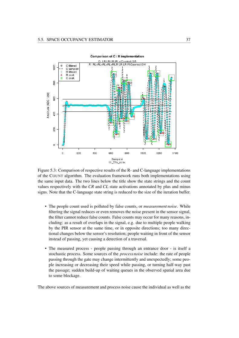
5.5. SPACE OCCUPANCY ESTIMATOR 37
Figure 5.3: Comparison of respective results of the R- and C-language implementationsof the COUNT algorithm. The evaluation framework runs both implementations usingthe same input data. The two lines below the title show the state strings and the countvalues respectively with the CR and CL state activations annotated by plus and minussigns. Note that the C-language state string is reduced to the size of the iteration buffer.
• The people count used is polluted by false counts, or measurement noise. Whilefiltering the signal reduces or even removes the noise present in the sensor signal,the filter cannot reduce false counts. False counts may occur for many reasons, in-cluding: as a result of overlaps in the signal, e.g. due to multiple people walkingby the PIR sensor at the same time, or in opposite directions; too many direc-tional changes below the sensor’s resolution; people waiting in front of the sensorinstead of passing, yet causing a detection of a traversal.
• The measured process - people passing through an entrance door - is itself astochastic process. Some sources of the processnoise include: the rate of peoplepassing through the gate may change intermittently and unexpectedly; some peo-ple increasing or decreasing their speed while passing, or turning half-way pastthe passage; sudden build-up of waiting queues in the observed spatial area dueto some blockage.
The above sources of measurement and process noise cause the individual as well as the

38 CHAPTER 5. IMPLEMENTATION
aggregate people count of any people counting system to be limited within the boundsof process noise, accuracy of the sensor and performance of the algorithms used.
For the purpose of this discussion we view the people counting process (Definition1) as a linear system, where the future state solely depends on the present occupancy(state) and the in and out counts (measurements) at discrete-time instance k.
Consider the model of spatial areas of Definition 10. Assume that for each area SA
and discrete-time instance k, the system collects N measurements of occupation definedas
occk,i = occk,i−1 +deltak, deltak,i = (ink,i−outk,i), 0≤ i < N,occ0 = 0 (5.5.1)
Then let us model the state space of each spatial area as a column vector
xk,i =
[occk,i
deltak,i
](5.5.2)
(w.l.g. we will subsequently drop the index i).
Further assume we have prior knowledge of the rate of change αk that deltak issubject to, at timesteps k. ak is assumed to be derived from previously establishedmeasurements or defined by the probability distribution function. Then we define theprocess model as
occk+1 = occk +αk ·deltak +w (5.5.3)
where k denotes the discrete-time instance and w is the process noise. Similarly, wedefine the measurement model as
deltak+1 = αk ·deltak +w (5.5.4)
Since we know α , it is reasonable to assume that we also have a notion of previousoccupation levels at time instance k. We can use this knowledge to (re-)initialize thestate by “injecting” a control input uk in case of drastic error of the state estimate (suchas an occupation less than zero). Transforming these equations into a linear differenceequation, we have process equation
xk+1 =
[0 αk0 αk
]xk +
[10
]uk +w (5.5.5)
and measurement equation
yk =
[01
]xk + v (5.5.6)
The process and noise covariance matrices w and v are assumed to be normally dis-tributed. These equations form the basis for the Kalman Filter to predict the true spaceoccupation.
A simulation was implemented using MATLAB based on the above assumptionsand equations as follows:
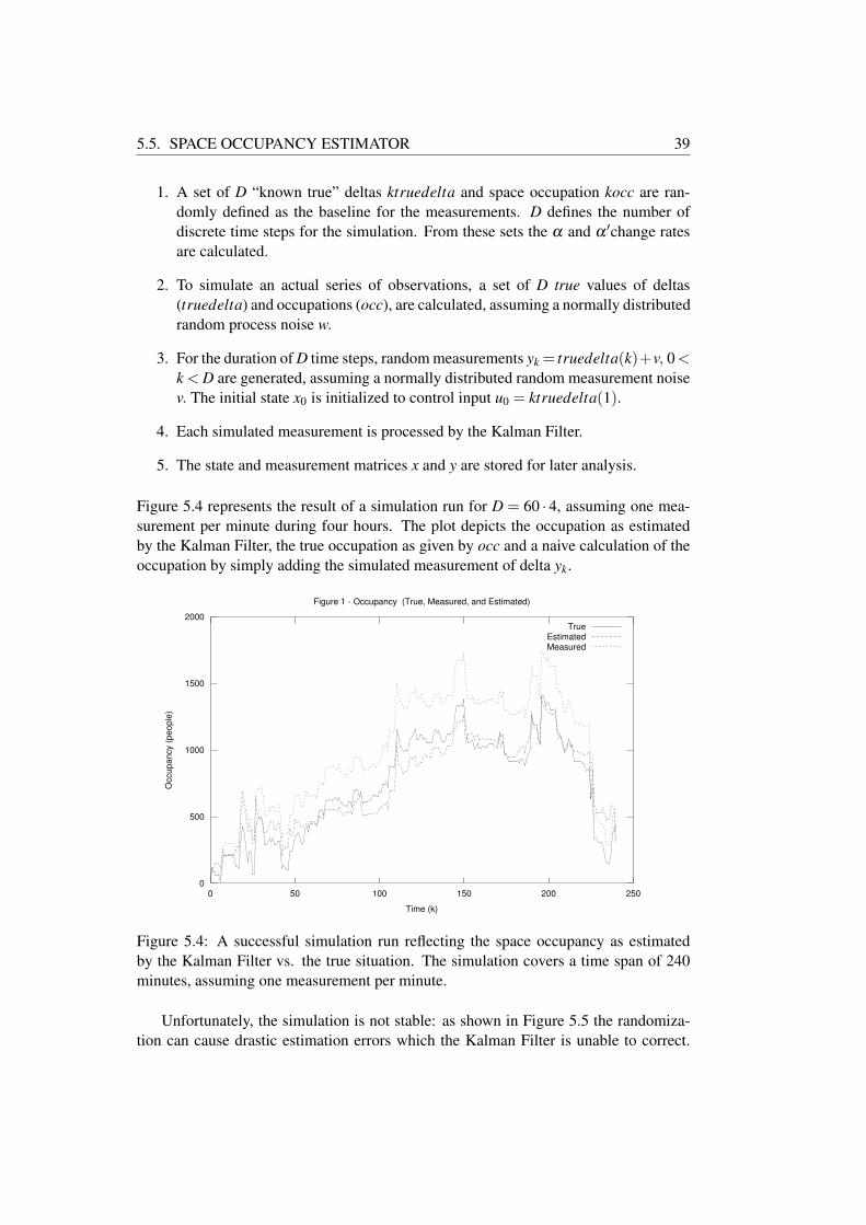
5.5. SPACE OCCUPANCY ESTIMATOR 39
1. A set of D “known true” deltas ktruedelta and space occupation kocc are ran-domly defined as the baseline for the measurements. D defines the number ofdiscrete time steps for the simulation. From these sets the α and α ′change ratesare calculated.
2. To simulate an actual series of observations, a set of D true values of deltas(truedelta) and occupations (occ), are calculated, assuming a normally distributedrandom process noise w.
3. For the duration of D time steps, random measurements yk = truedelta(k)+v, 0<k < D are generated, assuming a normally distributed random measurement noisev. The initial state x0 is initialized to control input u0 = ktruedelta(1).
4. Each simulated measurement is processed by the Kalman Filter.
5. The state and measurement matrices x and y are stored for later analysis.
Figure 5.4 represents the result of a simulation run for D = 60 · 4, assuming one mea-surement per minute during four hours. The plot depicts the occupation as estimatedby the Kalman Filter, the true occupation as given by occ and a naive calculation of theoccupation by simply adding the simulated measurement of delta yk.
0
500
1000
1500
2000
0 50 100 150 200 250
Occupancy (
people
)
Time (k)
Figure 1 - Occupancy (True, Measured, and Estimated)
TrueEstimatedMeasured
Figure 5.4: A successful simulation run reflecting the space occupancy as estimatedby the Kalman Filter vs. the true situation. The simulation covers a time span of 240minutes, assuming one measurement per minute.
Unfortunately, the simulation is not stable: as shown in Figure 5.5 the randomiza-tion can cause drastic estimation errors which the Kalman Filter is unable to correct.
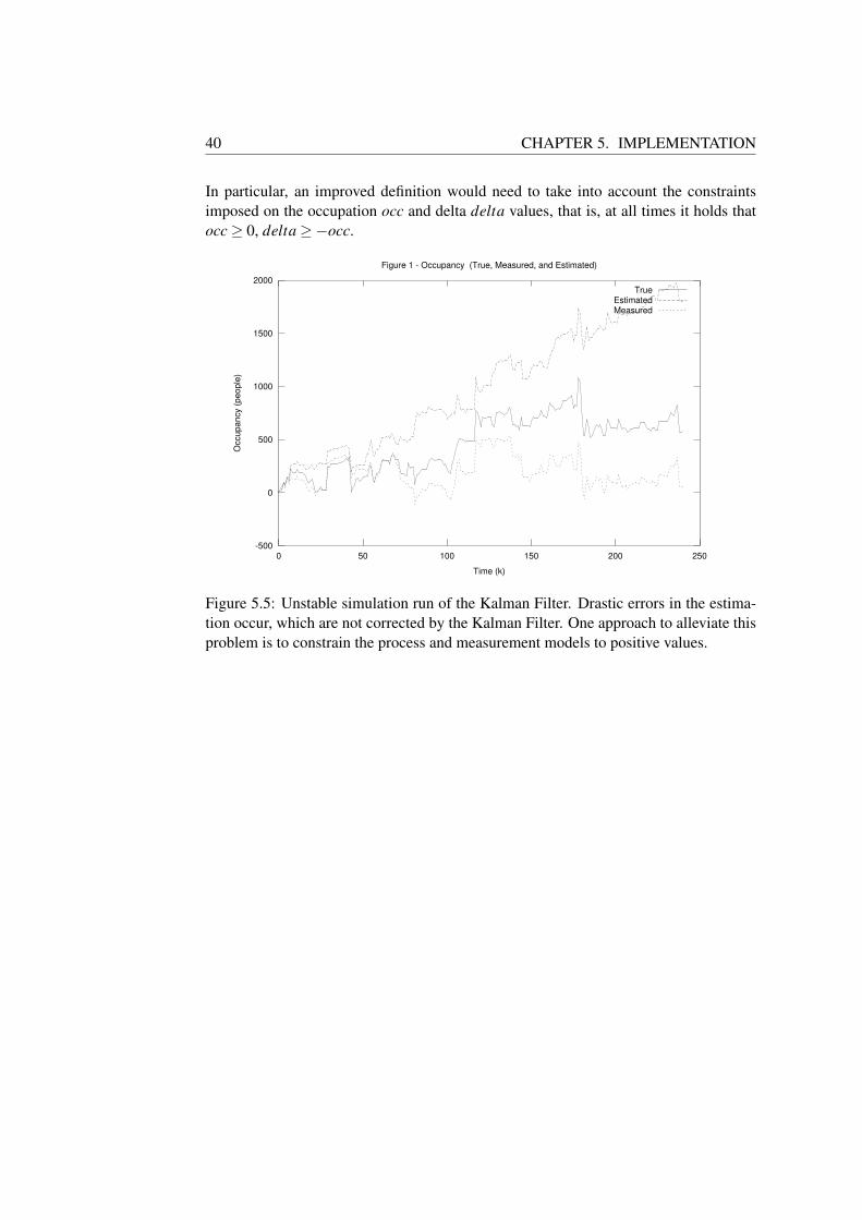
40 CHAPTER 5. IMPLEMENTATION
In particular, an improved definition would need to take into account the constraintsimposed on the occupation occ and delta delta values, that is, at all times it holds thatocc≥ 0, delta≥−occ.
-500
0
500
1000
1500
2000
0 50 100 150 200 250
Occupancy (
peo
ple
)
Time (k)
Figure 1 - Occupancy (True, Measured, and Estimated)
TrueEstimatedMeasured
Figure 5.5: Unstable simulation run of the Kalman Filter. Drastic errors in the estima-tion occur, which are not corrected by the Kalman Filter. One approach to alleviate thisproblem is to constrain the process and measurement models to positive values.
CHAPTER 6
Evaluation
To evaluate the algorithm and the PCSN’s performance, two distinct series of experi-ments were conducted. The first series was used to capture sensor data resulting fromseveral different movement patterns, including single-person passages and multiple peo-ple passing in line. For evaluation, the sensor output was subsequently processed by theC-implementations of the COUNT, PEAK and FILTER algorithms, using the test driver.Recall from Section 4.6 that the C implementation uses a restricted regular expressionas a realization of the FSM. To understand the impact of this limitation, one evaluationapplied the R implementation based on a fully specified DFA. All experiments weretimed in order to gauge the effect of higher rates of passages. The same experimentswere conducted using different timing parameters in order to simulate people walkingup-close or at larger distances from one person to the next. The evaluation was con-ducted in an office room, where the PCSN observed the room’s door to an adjacenthallway.
The second series of experiments consisted of two installation scenarios a,b of twoinstalled PCSNs. In scenario a, the PCSNs were installed at two opposite doors ofa meeting room, to count people walking in and out of this room. The nodes wereconfigured to periodically transmit (interval 1000ms), via the ZigBee RF link, theirrespective count values to the Monitor application set-up at the base station. In scenariob, the PCNSs were mounted to count people entries and exits at the main entranceof building ETZ at ETH. A concurrent manual count provided the baseline for lateranalysis.
6.1 COUNT Algorithm Performance
The following experiments were conducted for each of the time distances d indicatedin Table 6.1. The time distances give an approximate indication of how close to eachother the participants walked in line. The speed at which to walk was not regulated,however, the lower the distance in between passing events, the quicker each precedingindividual would make space for the next. A timer-based, toggling-LED installed inview of the participants indicated the time to start walking. As a result of slightly

42 CHAPTER 6. EVALUATION
differing reaction latencies to this signal among participants the time distances shouldbe considered approximate values.
Experiment [code] Time distance d between passing
(seconds)
One Person walking back and forth [1cd] 10,5,2.5,1
Queue of four people, all same direction [queue] 10,5,2.5,1,0.5
Queue of four people in each direction [cd] 10,5,2.5,1
Opposite passage of two or more people [od] 10,5,2.5,1
Table 6.1: Experiments
Consider Figure 6.1. The graph depicts the COUNT algorithm’s results cin, cout foreach experiment and in relation to expected count values cexpin, cexpout. The queueexperiment indicates good performance for distances of d = 10,2.5,1s, whereas theperformance for all other distances and experiments is rather poor. The algorithms’performance can be improved by changing the respective parameters. For reference, thealgorithm parameters for all experiments are provided in the appendix (Table 8.1).
Figure 6.1: Experiment results using algorithm parameters (a) of Table 8.1. The resultsare acceptable for some scenarios, however, fail in other scenarios.
Careful consideration of different parameter settings and the cut-off frequency ofthe Butterworth low-pass filter resulted in an improved performance as shown in Figure6.2. These results are mainly due to the parameters MAXDIST , PEAKWDT H, as wellas the filter’s cut-off frequency. The decrease in MAXDIST causes the algorithm toconsider an ignore state sooner, and widening PEAKWDT H results in improved peakdetection. Increasing the cut-off frequency of the low-pass filter helps in detecting morepeaks, in particular for distances smaller than 5s.

6.2. PCSN PERFORMANCE 43
Figure 6.2: Experiment results using improved parameters (b) of Table 8.1. In particu-lar, setting the cut-off frequency of the low-pass filter at 1Hz, and changing the COUNT
algorithm’s parameters to more appropriate values (e.g. MAXDIST, PEAWIDT H) pro-duces improved results for most scenarios and time distances.
The people count (y-axis) indicates the total count in each direction. Despite theimproved parameters, some problems persist. Let us consider distance d = 2.5s of thequeue experiment. In this case, the cut-off frequency c f = 1Hz causes the filter to“over-smooth” the signal, and in turn the algorithm misses to consider relevant peaks.As a result, the directional counts are invalid, and the total count overshoots by 25%.A similar pattern is responsible for the result at distance d = 0.5s. Both cases can bealleviated by setting a higher cut-off frequency, and by applying the regular expressionas implemented by the R version of the COUNT algorithm. However, these changesresult in a much diminished performance for all other experiments.
Consider Figure 6.3 for a normalized comparison of algorithm performance at vari-ous cut-off frequencies and respective parameters. Across experiments, the parameters(b) in Table 8.1 work best. For some installation scenarios parameters (c) might be ap-plicable, e.g. in an area of high-frequency pedestrian or passenger volumes and wherethere is mostly one-directional traffic.
6.2 PCSN Performance
For scenario a, two PCSNs were configured using parameters (a) of Table 8.1. Cor-responding to the respective evaluation of the algorithms (Figure 6.1), the combinedcounts were accurate for distances t = 10,5s, and increasingly erroneous for other dis-tances. Note that people left the room at timed intervals, while the distances at theroom entrance were chosen at random by the participants arriving in line. The doors are2.1mx0.8m (height x width) in dimension, which is within the assumed specifications
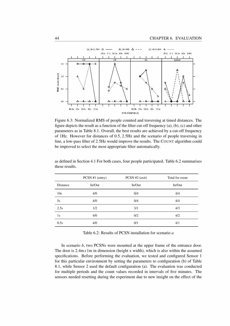
44 CHAPTER 6. EVALUATION
Figure 6.3: Normalized RMS of people counted and traversing at timed distances. Thefigure depicts the result as a function of the filter cut-off frequency (a), (b), (c) and otherparameters as in Table 8.1. Overall, the best results are achieved by a cut-off frequencyof 1Hz. However for distances of 0.5, 2.5Hz and the scenario of people traversing inline, a low-pass filter of 2.5Hz would improve the results. The COUNT algorithm couldbe improved to select the most appropriate filter automatically.
as defined in Section 4.1 For both cases, four people participated. Table 6.2 summarisesthese results.
PCSN #1 (entry) PCSN #2 (exit) Total for room
Distance In/Out In/Out In/Out
10s 4/0 0/4 4/4
5s 4/0 0/4 4/4
2.5s 1/2 3/1 4/3
1s 4/0 0/2 4/2
0.5s 4/0 0/1 4/1
Table 6.2: Results of PCSN installation for scenario a
In scenario b, two PCSNs were mounted at the upper frame of the entrance door.The door is 2.4mx1m in dimension (height x width), which is also within the assumedspecifications. Before performing the evaluation, we tested and configured Sensor 1for this particular environment by setting the parameters to configuration (b) of Table8.1, while Sensor 2 used the default configuration (a). The evaluation was conductedfor multiple periods and the count values recorded in intervals of five minutes. Thesensors needed resetting during the experiment due to new insight on the effect of the

6.2. PCSN PERFORMANCE 45
environment. Due to a technical problem and the battery running empty, Sensor 2’svalues were only recorded for one period. Table 6.3 summarises the results of scenariob.
Time Manual Count Sensor 1 Count Sensor 2 Count Notes
0:00 4 / 3 3 / 4 not recorded
0:05 4 / 1 6 / 4 not recorded left: group
0:10 1 / 2 7 / 4 not recorded
0:15 2 / 3 12 / 4 not recorded
0:20 1 / 3 13 / 4 not recorded right: group
0:25 0 / 2 16 / 4 not recorded
Total 12 / 14 16 / 4 not recorded
Reset sensor regular expression Rle f t
0:30 2 / 2 3 / 0 0 / 1
0:35 2 / 3 4 / 0 0 / 2 right: group
0:40 2 / 1 7 / 0 1 / 2
0:45 1 / 2 10 / 0 2 / 2
Total 6 / 6 7 / 0 2 / 2
Reset sensor viewing angle to 50° /20°
0:45 3 / 1 3 / 1 out of battery
0:55 2 / 0 5 / 1 out of battery
1:00 4 / 4 9 / 2 out of battery right: group
1:05 4 / 4 13 / 2 out of battery right: group
1:10 4 / 1 16 / 4 out of battery
Total 14 / 9 16 / 4 out of battery
Table 6.3: Results of the evaluation at a building entrance door. The results indicate theneed for further analysis of the impact of differences in temperature on the two sides ofthe sensor and the traversal pattern of groups of people.
The first evaluation period clearly showed that the directional counts did not work asexpected. Instead, the sensors counted some traversals as if they happened in the samedirection. Closer inspection of the entrance area provided the insight that one side ofthe entrance door was warmed by sunlight. As a result, the signal by the dual-elementsensors were biased towards the cooler side, and thus were wrongly interpreted by thealgorithm.

46 CHAPTER 6. EVALUATION
In order to compensate for this effect, we changed the covering of the PIR sensorssuch that the field of view included up to 40° on the cooler side, while we limited theother side to 20°. In a first attempt, the algorithm’s regular expression was changed tocompensate for the temperature difference by setting Rle f t = LL?R?. Using this expres-sion, however, resulted in lower sensitivity on the side warmed by sun-light. The nextstep was to reset the sensor’s viewing angle, which improved the directional count, butstill did not yield the accuracy expected.
It is apparent from the data that the moving pattern for groups is different than inthe previous section. We assumed that groups would pass the sensor in line. The exper-iments conducted in this scenario indicate, in contrast, that groups approach the sensorby two or more people at once, and only then start to pass the sensor one-by-one. Wedid not analyse the sensor signal in this particular scenario. The count values indicatethat group passages are either counted as none, or as two people. Concluding from thisexperiment, there is a need to further analyse the impact of differences in temperatureon the two sides of the sensor, to better understand the impact of the environment (e.g.door height, room height), and the traversal pattern of groups of people.
CHAPTER 7
Conclusion
The goal of this thesis was to develop a distributed people counting system by inexpen-sive hardware. Dual-element PIR sensors were chosen for their simplicity and effec-tiveness. This type of sensor has several advantages: it operates at low-power levels,no ambient light source is required and the effects of slow changes to the environmentare cancelled automatically. In contrast to other approaches used for people counting,e.g. cameras or infrared arrays, interpreting a PIR sensor signal imposes relatively lowrequirements in regards to compute power.
We have considered the people counting problem from different perspectives. Thisincluded the development of algorithms to parse PIR sensor signals, the collection ofresults from a distributed network of sensor nodes, and the estimation of a total spaceoccupancy based on such measurements. The algorithms developed apply a novel ap-proach to the people counting problem. In particular, the application of a configurableFSM, based on regular expressions and combined with several other parameters enablesa sensor node to adopt to a range of deployment scenarios. The prototype implementa-tion of these algorithms on sensor nodes demonstrated their feasibility for deploymentin a wireless sensor network. Using a number of base stations as the gateway to theweb-based data collection server, a setup covering larger areas is possible.
7.1 Future Work
While the evaluation demonstrates the adaptability of the people counting algorithmto various movement patterns, it reveals several open problems. In a real-life setting,people cannot be expected to pass an observed passage at presumed or timed intervals.In consequence, the FILTER and COUNT algorithms should be able to detect the rate ofpassages, and adopt the algorithm parameters and filter strategy automatically.
Further, the COUNT algorithm should be changed such that it automatically com-pensates for temperature differences on either side of the sensor, e.g. by estimating asignal bias to either side, and by evaluating the relative maximum strength of the sensorsignal amplitude. The algorithm could also be improved to derive and take into accounta probabilistic estimate in relation to the ratio of directional changes it detects.

48 CHAPTER 7. CONCLUSION
In some scenarios the calculated total occupancy for some observed space may bewithin acceptable limits of accuracy, despite each sensor node’s count values. Stochasticstate estimation combined with previously recorded statistics can be applied to solve thisproblem in principle. However, our solution approach using a linear Kalman Filter isnot sufficiently stable. Future work should include evaluation of non-linear estimationmodels.
The prototype implementation of the PCSN does not make use of the dynamic char-acteristics of the counting algorithms. While the prototype code exposes parametersto configure the various operating modes and to change run-time parameters, effectingthese changes requires re-programming of each sensor node by USB cable. For real-istic and productive use, the PCSN needs to be extended such that the algorithms canbe configured through ZigBee. That is, the PCSN requires a management mode, whichcan be activated from the base station in order to dynamically apply changes to filtercoefficients and other parameters. This includes the extension of the iterative regularexpression algorithm to support character repetition and grouping.
The ZigBee protocol was chosen for its low-rate, low-power capabilities. The pro-totype PCSNs do not realize a low-power mode, and hence are inefficient to operateon battery. In a productive scenario, a low-power mode is required to include both theCPU and the RF module. The PIR sensors ability to detect motion independent of a hostprocessor could be exploited as a trigger to wake-up the node.
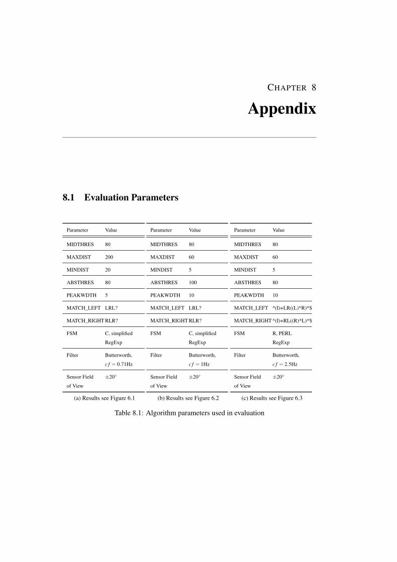
CHAPTER 8
Appendix
8.1 Evaluation Parameters
Parameter Value
MIDTHRES 80
MAXDIST 200
MINDIST 20
ABSTHRES 80
PEAKWDTH 5
MATCH_LEFT LRL?
MATCH_RIGHT RLR?
FSM C, simplified
RegExp
Filter Butterworth,
c f = 0.71Hz
Sensor Field
of View
±20°
(a) Results see Figure 6.1
Parameter Value
MIDTHRES 80
MAXDIST 60
MINDIST 5
ABSTHRES 100
PEAKWDTH 10
MATCH_LEFT LRL?
MATCH_RIGHT RLR?
FSM C, simplified
RegExp
Filter Butterworth,
c f = 1Hz
Sensor Field
of View
±20°
(b) Results see Figure 6.2
Parameter Value
MIDTHRES 80
MAXDIST 60
MINDIST 5
ABSTHRES 80
PEAKWDTH 10
MATCH_LEFT ^(I)+LR((L)*R)*$
MATCH_RIGHT ^(I)+RL((R)*L)*$
FSM R, PERL
RegExp
Filter Butterworth,
c f = 2.5Hz
Sensor Field
of View
±20°
(c) Results see Figure 6.3
Table 8.1: Algorithm parameters used in evaluation

50 Appendix
8.2 Technology Overview
The following table provides a list of all third-party technology used for the prototypeimplementation.
Area Description Details [software license] Vendor/Source
Hardware Sensor Node
Prototype
Name: Arduino UNOMicrocontroller: ATmega328Operating Voltage: 5VFlash Memory: 32KB, SRAM: 2KBEEPROM: 1KB
Clock Speed: 16MHz
SparkFun Electronicswww.sparkfun.com
Product ID 9950
Sensor Node
Testboard
Microcontroller: ATmega168Operating Voltage: 5VFlash Memory: 16KB, SRAM: 1KB
EEPROM: 512 bytes
Dshop Electronicswww.dshop.ch
Product ID ARD2K
Sensor Node
RF Module
ZigBee, 3V
break-out
regulated
DigiKey XBee Series 1Frequency: 2.4GHzStandard: IEEE 802.15.4Operating Voltage: 3.3V, 50mAData Rate: 250kbps
Range: 100m
SparkFun Electronicswww.sparkfun.com
Product ID 8664 (XBee module),
9132 (XBee break-out regulated)
PIR Sensor Operating Voltage: 3-12V / 1.4mARange: 4-12mCoverage angle: v :±30°/h :±50°
Signal bandwidth: 0.2Hz−10Hz
Conrad Electronicswww.conrad.ch
Product ID 172500-62
Software Sensor Node Arduino Development EnvironmentGCC 4.4.5 [GPL]avr-libc 1.6.8 [Copyleft]
XBee API 0.2 [GPL]
www.arduino.comhttp://gcc.gnu.org/http://www.nongnu.org/avr-libc
http://code.google.com/p/xbee-
arduino/
Sensor
Monitor
Processing 1.5 [GNU]OpenJDK Java 1.6 [GNU]
Xbee API 0.9 [GNU]
http://processing.org/http://openjdk.java.net/
http://code.google.com/p/xbee-api/
Data
Collection
Server
Python 2.6.6 [PSF]appengine-rest-server [Apache]pyrest [MIT]
mpmath [BSD]
http://python.org/http://code.google.com/p/appengine-rest-server/http://code.google.com/p/pyrest/
http://code.google.com/p/mpmath/
State
Estimator
kalmanf.m [MATLAB Central] www.mathworks.com
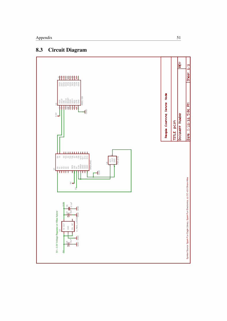
AR
DU
INO
V_R
EG
_LD
OS
MD
GN
D
10uF
0.1u
F
GN
DG
ND
10uF
GN
D
XB
EE
-1B
3
9V
3.3V
PIR
-STD
GN
D
GN
D
RX TX D2
*D3
D4
*D5
*D6
D7
D8
*D9
*D10
*D11
D12
D13
A0
A1
A2
A3
A4
A5
VIN
RE
S
5V AR
EF
GN
DG
ND
GN
D
3.3V
U1
IN GN
DOU
T
U2 E
NB
P
C4
C5
C6
VD
D1
DO
UT
2
DIN
3
DIO
124
RE
SE
T5
RS
SI
6
DIO
117
RE
S8
DTR
9
GN
D10
DIO
411
CTS
12D
IO9
13R
ES
14D
IO5
15R
TS16
DIO
317
DIO
218
DIO
119
DIO
020
U3
VC
C3
GN
D1
OU
T2
U4
5V
5V
3.3V
Sym
bol S
ourc
e: S
park
Fun
Eag
le L
ibra
ry, S
park
Fun
Ele
ctro
nics
, (c)
CC
v3.
0 S
hare
-Alik
e
5V >
3.3
V V
olta
ge R
egul
ator
on
XB
ee X
plor
er
Appendix 51
8.3 Circuit Diagram

52 Appendix
8.4 Implementation Reference
The following table provides a summary of all implemented program modules and func-tions by the validation framework and the prototype.
Area Program/Function Description Programming
Language
Validation
Framework
(Simula-
tion)
countlib.r R implementation of algorithms and helper functions R
ex.run() Run the algorithms for experiment data using
different filters, display count results in tabular
format
R
ex.plotbyfilter() Run algorithms using different filters, plot results R
testccode Run R algorithms and visually compare output to C
implementation’s result
R
hots() Identify peaks in signal using standard deviation
around sw points
R
count() Count peaks according to FSM specification (several
variants of count exist: count_fix, count_fsm,
count_dynfsm) for execution of simple algorithm,
hard coded FSM, regular expression based FSM)
R
count_c() R implementation of C version of count() (restricted
Regular Expression)
R
filter.CArma R implementation of C version of filter() R
filter2c Output C data structure of coefficients of a R filter
defined by the signal package
R
logger.sh Logging routine to act as counterpart to the sensor
node’s LOGGER mode
Bash
Sensor
Node
filter.h Algorithm implementation for C-language C
hots() Identify peaks in signal using standard deviation
around sw points
C
count() Count peaks according to simplified regular
expression
C
filter() IIR signal filter implementation C
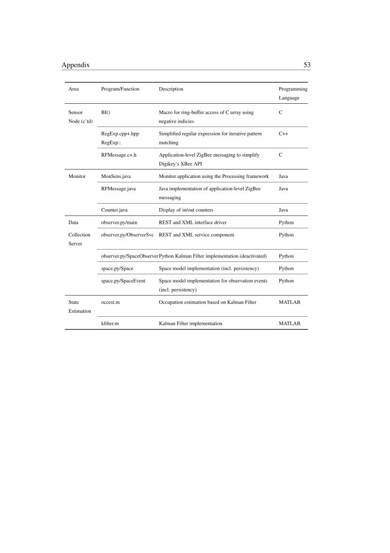
Appendix 53
Area Program/Function Description Programming
Language
Sensor
Node (c’td)
BI() Macro for ring-buffer access of C array using
negative indicies
C
RegExp.cpp+.hpp
RegExp::
Simplified regular expression for iterative pattern
matching
C++
RFMessage.c+.h Application-level ZigBee messaging to simplify
Digikey’s XBee API
C
Monitor MonSens.java Monitor application using the Processing framework Java
RFMessage.java Java implementation of application-level ZigBee
messaging
Java
Counter.java Display of in/out counters Java
Data observer.py/main REST and XML interface driver Python
Collection
Server
observer.py/ObserverSvc REST and XML service component Python
observer.py/SpaceObserverPython Kalman Filter implementation (deactivated) Python
space.py/Space Space model implementation (incl. persistency) Python
space.py/SpaceEvent Space model implementation for observation events
(incl. persistency)
Python
State
Estimation
occest.m Occupation estimation based on Kalman Filter MATLAB
kfilter.m Kalman Filter implementation MATLAB
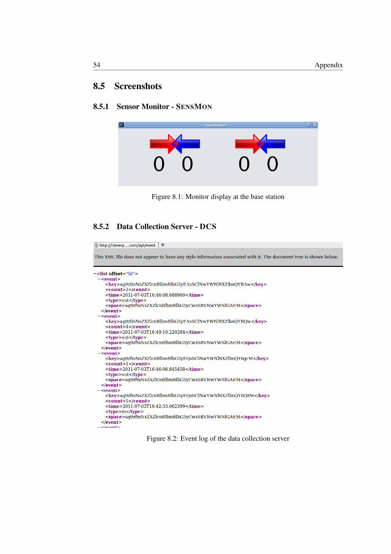
54 Appendix
8.5 Screenshots
8.5.1 Sensor Monitor - SENSMON
Figure 8.1: Monitor display at the base station
8.5.2 Data Collection Server - DCS
Figure 8.2: Event log of the data collection server

Bibliography
[1] T. Teixeira and A. Savvides. Lightweight People Counting and Localizing in In-door Spaces Using Camera Sensor Nodes. In Proceedings of Conference on Dis-tributed Smart Cameras, 2007, ICDSC, pages 36 –43.
[2] S. Velipasalar, Ying-Li Tian, and A. Hampapur. Automatic Counting of Inter-acting People by using a Single Uncalibrated Camera. In Proceedings of IEEEInternational Conference on Multimedia and Expo, 2006, pages 1265 –1268.
[3] Quanbin Chen, Min Gao, Jian Ma, Dian Zhang, Lionel M. Ni, and Yunhao Liu.Moving Object Counting using Ultrasonic Sensor Networks. International Journalof Sensor Networks, 2008, pages 55–65, volume 3.
[4] K. Hashimoto, K. Morinaka, N. Yoshiike, C. Kawaguchi, and S. Matsueda. PeopleCount System using Multi-Sensing Application. In Proceedings of InternationalConference on Solid State Sensors and Actuators, 1997. TRANSDUCERS, pages1291 –1294, volume 2.
[5] P. Zappi, E. Farella, and L. Benini. Enhancing the Spatial Resolution of PresenceDetection in a PIR based Wireless Surveillance Network. In Proceedings of IEEEConference on Advanced Video and Signal Based Surveillance, 2007, AVSS, pages295 –300.
[6] S. Meyn, A. Surana, Yiqing Lin, S.M. Oggianu, S. Narayanan, and T.A. Frewen.A Sensor-Utility-Network Method for Estimation of Occupancy in Buildings. InProceedings of IEEE Conference on Decision and Control, held jointly with theChinese Control Conference, 2009, CDC/CCC, pages 1494 –1500.
[7] Emi Mathews and Axel Poigné. Evaluation of a "Smart" Pedestrian CountingSystem based on Echo State Networks. Journal on Embedded Systems, EURASIP,pages 8:1–8:9, January.
[8] Muhammad Tahir, Peter Hung, Ronan Farrell, Sean McLoone, and Tim McCarthy.Lightweight Signal Processing Agorithms for Human Activity Monitoring usingDual PIR-Sensor Nodes. In Proceedings of the China-Ireland information andcommunications technologies conference, CCIT, 2009, pages 150–156.
[9] Lin Gu, Dong Jia, Pascal Vicaire, Ting Yan, Liqian Luo, Ajay Tirumala, Qing Cao,Tian He, John A. Stankovic, Tarek Abdelzaher, and Bruce H. Krogh. LightweightDetection and Classification for Wireless Sensor Networks in Realistic Environ-ments. In Proceedings of Conference on Embedded networked sensor systems,2005, SenSys, pages 205–217.

56 Appendix
[10] Robert Tomastik, Satish Narayanan, Andrzej Banaszuk, and Sean Meyn. Model-Based Real-Time Estimation of Building Occupancy During Emergency Egress.In Pedestrian and Evacuation Dynamics 2008, pages 215–224. Springer, 2010.
[11] V. Vaidehi, S. Vasuhi, K.S. Ganesh, C. Theanammai, N.T. Naresh Babu, N. Uthi-ravel, P. Balamuralidhar, and G. Chandra. Person Tracking using Kalman Filter inWireless Sensor Network. In Proceedings of Second International Conference onAdvanced Computing (ICoAC), 2010, pages 60 –65.
[12] Jian-Shuen Fang, Qi Hao, David J Brady, Mohan Shankar, Bob D Guenther,Nikos P Pitsianis, and Ken Y Hsu. Path-dependent Human Identification usinga Pyroelectric Infrared Sensor and Fresnel-lens Arrays. Optics Express, pages609–624, volume 14, 2006.
[13] Steven Smith. Digital Signal Processing, pages 107–111, 116–121, 319–322,333–342. Newnes, 2003.
[14] Peter Linz. An Introduction to Formal Languages and Automata, Fifth Edition,pages 38–46. Jones & Bartlett Learning, 2011.
[15] Christos G. Cassandras and Stephane Lafortune. Introduction to Discrete EventSystems, pages 23–31,61–72. Springer, 2007.
[16] Greg Welch and Gary Bishop. An Introduction to the Kalman Filter. Universityof North Carolina at Chapel Hill, Department of Computer Science, 1995.
[17] Zhiqiang Zhang, Xuebin Gao, J. Biswas, and Jian Kang Wu. Moving TargetsDetection and Localization in Passive Infrared Sensor Networks. In Proceedingsof International Conference on Information Fusion, 2007, pages 1 –6.
[18] P. Zappi, E. Farella, and L. Benini. Pyroelectric InfraRed Sensors based DistanceEstimation. In Proceedings of IEEE Sensors, 2008, pages 716 –719.
[19] G. Palshikar. Simple Algorithms for Peak Detection in Time-Series. In Proceed-ings of 1st IIMA International Conference on Advanced Data Analysis. BusinessAnalytics and Intelligence, 2009.
[20] Tom Short. R Signal Processing Package, 2011. R package version 0.6-2.