distributed operations planning in the lumber …distributed operations planning in the lumber...

______________________________ Distributed Operations Planning in the Lumber Supply Chain: Models and Coordination

Jonathan Gaudreault Pascal Forget Jean-Marc Frayret Alain Rousseau Sophie D’Amours

February 2009

CIRRELT-2009-07

Distributed Operations Planning in the Lumber Supply Chain: Models and Coordination

Jonathan Gaudreault1,2,*, Pascal Forget1,3, Jean-Marc Frayret1,2, Alain Rousseau1, Sophie D’Amours1,3

1 Interuniversity Research Centre on Enterprise Networks, Logistics and Transportation

(CIRRELT) 2 Mathematics and Industrial Engineering Department, École Polytechnique de Montréal, C.P.

6079, succursale Centre-ville, Montréal, Canada H3C 3A7 3 Département de génie mécanique, Université Laval, Pavillon Adrien-Pouliot, 1065, avenue de la

médecine, Québec, Canada G1V 0A6 Abstract. Agent-based technology provides a natural approach to model supply chain

networks. Each production unit, represented by an agent, is responsible for planning its

operations and uses communication to coordinate with the others. In this paper, we study

a softwood lumber supply chain made of three planning units (sawing unit, drying unit and

finishing unit). We define the problems and propose agent-specific mathematical models

to plan and schedule operations. Then, in order to coordinate these plans between the

three agents, we propose different coordination mechanisms. Using these developments,

we show how an agent-based simulation tool can be used to integrate planning models

and evaluate different coordination mechanisms.

Keywords. Distributed operations planning, coordination, optimization, agent, supply

chain, lumber.

Acknowledgements. This work was funded by the FORAC Research Consortium and the

Natural Sciences and Engineering Research Council of Canada (NSERC). The authors

would also like to acknowledge the impressive work of many FORAC research assistants

who have worked on the development of the agent-based platform.

Results and views expressed in this publication are the sole responsibility of the authors and do not necessarily reflect those of CIRRELT. Les résultats et opinions contenus dans cette publication ne reflètent pas nécessairement la position du CIRRELT et n'engagent pas sa responsabilité. _____________________________

* Corresponding author: [email protected] Dépôt légal – Bibliothèque et Archives nationales du Québec, Bibliothèque et Archives Canada, 2009

© Copyright Gaudreault, Forget, Frayret, Rousseau, D’Amours and CIRRELT, 2008

1. INTRODUCTION

Canadian lumber companies are confronted with the need to reengineer the way they manage and plan their supply chain operations. Supply chains are global networks of organizations where material and information flow in many directions within and across organizational boundaries through complex business networks of suppliers, manufacturers and distributors, to the external customers. These organizations can be part of the internal supply chain, which consists of members of the same company, or part of the external supply chain, which includes members of different companies. They must all cooperate to exchange materials and information to maximize customer satisfaction at the lowest possible cost.

In that regard, the lumber supply chain is similar to other industries: lumber material flows from forest contractors, to sawing facilities, to value-added mills (referred to as secondary transformation), and through the many channels of distributors and wholesalers to finally reach the markets. However, lumber operational planning represents a major challenge. Unlike the traditional manufacturing industry which has a convergent product structure (i.e., assembly), the lumber industry needs to master industry-specific operational processes. These are characterized by: (1) a divergent product structure (i.e., trees are broken down into many products), (2) the highly heterogeneous nature of its raw material and (3) radically different planning problems must be solved by each production center.

Distributed planning is an interesting approach for supply chain operational planning since it enables the use of specific optimization strategies and information available only locally. Unlike centralized planning approaches, which generally cannot take into account specific operational details, distributed planning makes it possible to create detailed models of specific planning problems.

Building on Gaudreault et al. (2008), this paper aims to propose planning models for the lumber production units and to compare different coordination mechanisms. In Section 2, we present a description of the softwood lumber production processes and planning strategy used by practitioners. Next, in Section 3, a literature review is provided on lumber planning, supply chain and coordination. Then, we propose in Section 4 a distributed planning system, including specific planning models for each production unit and coordination mechanisms to ensure coherence between agents. Section 5 presents the experimentation of the models and coordination mechanisms in an industrial application. We show how agent-based tools can be used to compare them. Finally, Section 6 concludes the paper.

2. SOFTWOOD LUMBER PRODUCTION AND PLANNING

2.1 Production Units

This section introduces the three different production units involved in softwood lumber production: (1) the sawing facility, where logs are cut into various sizes of rough pieces of lumber; (2) the drying facility, which reduces the lumber moisture content and (3) the finishing facility, where lumber is planed (surfaced), trimmed and sorted. Figure 1 presents the different production units.

Figure 1. Production units and products in a lumber supply chain


CIRRELT-2009-07 1

This paper does not look into the log supply problem. In practice, forest is harvested by entrepreneurs responsible for felling trees and crosscutting them into logs. We consider that log supply to the sawing unit is known, which is the current practice in the industry.

2.1.1 Sawing Unit

Logs often remain for long periods in a sawmill yard before being processed. They are stored in huge lots according to certain physical characteristics (species, length, average diameter, etc.), each lot representing a specific class of logs.

Logs are then broken down into various sizes of rough pieces of lumber. Different dimensions of lumber will be obtained at the same time from a single log, which is called co-production. Most of the time, sawmills have access to data regarding past production, allowing them to forecast the expected quantities of the different types of lumber to be produced from a specific quantity of logs of a given log class. This information defines a production matrix (Figure 2). Arcs show the quantity of each type of lumber expected when sawing a given volume from a specific log class.

Figure 2. Example of a production matrix

In most sawmills, the production line can be set up in different modes; each setup is associated to a specific production matrix. This gives the production manager some control over the production output mix. Certain log classes may be incompatible with certain setups. For example, in most sawmills fir and spruce cannot be processed in the same production shift; they are associated with different setups. Therefore, the planning decisions the production manager must make are the following: (1) decide how the plant will be set up for each production shift, and (2) decide which quantities of each log class to consume at each production shift.

Once logs are sawn, green pieces of lumber are assembled into bundles of the same dimension (2”x3”, 2”x4”, etc.) and length (8-foot, 12-foot, 16-foot, etc.), and generally of the same species (spruce, fir, etc.) in order to be dried.

2.1.2 Drying Unit

Lumber drying is a transformation operation which aims at decreasing the lumber moisture content in order to meet customer requirements. These requirements are usually specified by industry standards, although some customers may require specific levels of moisture content. Softwood lumber drying is a rather complex process to carry out. It takes days and it is done in batches within large kiln dryers. Bundles of lumbers of different length can be dried in the same batch (e.g. 8-foot and 16-foot), but lumbers must be of the same dimension and species (although there are some exceptions). A bundle must be assembled as a rectangular prism filling the kiln dryer almost entirely. There are many constraints related to the stability of this stacking. For these reasons, each sawmill defines its own set of loading patterns that can be used. Figure 3 shows two examples of loading patterns.


CIRRELT-2009-07 2

Figure 3. Examples of small loading patterns (actual kilns and patterns contain a few hundred bundles)

Under certain circumstances, special sections of the wood yard may be used to perform air drying. Air drying, which precedes kiln drying, may take several weeks but allows the reduction of the drying time in the kiln. Air drying also plays a role in increasing the overall quality of the finished product (obtained after finishing).

For a given batch of green lumber, there are different possible alternative operations that can be used for air-drying and kiln-drying. Figure 4 presents an example of four possible alternative combinations of operations. For air drying, these are mostly differentiated according to their durations. For kiln operations, they are different w.r.t. air temperature, humidity parameters, and duration. The planning decisions for this production unit are the following: (1) what drying activities to perform, (2) what loading pattern to use, and (3) when to perform them.

Figure 4. Example of drying processes available for a given batch of lumber

2.1.3 Finishing Operations

At the finishing facility, lumbers are first planed (or surfaced). They are then sorted according to their grade (i.e. quality) with respect to the residual moisture content and physical defects. Lumber may be trimmed in order to produce a shorter lumber of a higher grade and value. This process is usually optimized by hardware to produce products with the highest value, with no consideration for the actual customer demand. This causes the production of multiple product types at the same time (co-production) from a single product type in input (divergence). It is important to note that the co-production cannot be avoided from a planning point of view; it is embedded within the transformation process. It is common to obtain more than 20 different types of products from a single product. The expected products mix to obtain from a batch depends on the drying process used. Therefore, in the planning models introduced hereafter, we consider the output product associated with each of the drying processes (path in Figure 4) as a different kind of input for the finishing process.

There is also a setup cost each time the facility processes a different dimension (e.g. from 2”x3” to 2”x6”). Consequently, most sawmills allow such a setup only between production shifts as they prefer campaigns (a batch of products of the same dimension but variable length) with a duration of more than one shift.

To sum up, the decisions that must be taken in order to plan the finishing operations are the following: (1) which campaign to realize (i.e. which lumber dimensions), (2) when and for how long and (3) for each campaign, which quantities of each length to process. Figure 6 shows a simple example of a production plan, including the campaigns (2”x3”, 2”x6” and 2”x4”) and the time spent on each length.


CIRRELT-2009-07 3

Figure 5. Production plan for a finishing line for six consecutive production shifts

2.2 Lumber Production Planning

Due to the highly heterogeneous nature of the resource and the inherent complexity of forecasting production throughput, the dominant thinking in the North American lumber industry is to produce the maximum volume with the available resource. This can be identified as a push production mode, where demand from specific clients is not taken into account. Production is oriented towards large batches to take advantage of economy of scale, resulting in large inventories, low flexibility and low agility. The production manager has as main objective to feed the production line continuously, in order to maximize the production rate and the throughput. He also tries to forecast the quantity of output products as precisely as possible. This way, he can give clear information to the sales department about what will be available and when.

While this planning approach has the advantage of maximizing the throughput value, it does not take client needs into account. On-hand inventory can be different from what final clients really want, leading to missed sales opportunities. Also, when unforeseen events occur (such as kiln dryer breakdown, unplanned maintenance or power outage) production can be very different from what has been forecasted. In these cases, it becomes difficult to fulfill promised deliveries.

Using their current planning tools (generally in-house spreadsheet applications), it is difficult for production managers to adjust a production plan that proposes a solution to such problems. Also, they cannot try multiple alternative planning scenarios. This is why some Canadian lumber producers are investigating the possibility of evolving from a push production mode to a pull mode.

In order to design such a pull production system, some characteristics of the problem must be taken into account. For example, it takes days to produce a batch of green lumber that is ready to be dried because of co-production at the sawing unit. The relatively large size of kiln dryers and the constraint to dry similar products together also imposes some important production lead times. Furthermore, due to co-production at the finishing unit, a single batch of green lumber to be dried and finished contributes to fulfill many customer orders for different product types. Also, because the volume of each customer order for a specific product is usually larger than the amount produced with one single batch, many batches are usually needed to fulfill one particular need. These specific issues have raised the need for a tightly integrated process planning and scheduling (Bartak et al, 2002).

3. LITERATURE REVIEW

3.1 Lumber Production Planning

Few authors have worked on the specific problem of softwood lumber production planning. Among them, Maness et al (1993) have proposed a mixed programming model that simultaneously determines the optimal bucking and sawing policies based on demand and final product price (integration of stem bucking and log sawing). This model was later modified to handle several periods (Maness et al, 2002). These works focus on the identification of new cutting patterns/policies.

Taking a more global view of the supply chain, Singer et al (2007) recently presented a model for optimizing planning decisions in the sawmill industry. They modeled a simplified internal supply chain, including two transformation stages and two inventory stages. The objective was to demonstrate how collaboration can benefit the partners, by transferring timber and using the competitive advantages of each. Other interesting studies have been presented about the integrated supply chain planning in the wood furniture industry (Ouhimmou et al, 2005) and in the OSB panel industry (Feng et al, 2008).

3.2 Supply Chains Planning

Supply chain operations planning is a complex issue. Companies usually deal with this by implementing and using information and decision support systems, which address various planning tasks. Some companies also adopt just-in-time approaches to control the pace of production and replenishment. When organizational units are part of the same company, centralized information and planning systems are sometimes used. Gathering information in a centralized management


CIRRELT-2009-07 4

system and redistributing plans can ensure synchronization and optimization of plans. Decision support systems, such as Advanced Planning and Scheduling (APS) systems are sophisticated sets of decision support applications using operational research (OR) techniques to find solutions to complex planning problems (Frayret, 2002). APS systems are considered by many as state of the art manufacturing and supply chain planning and scheduling practices. The reader is referred to Stadtler (2005) and Stadtler et al (2005) for a thorough description of APS.

However, even in an internal supply chain, the planning problem is complex and difficult to handle. In fact, currently available software solutions generally do not provide the necessary support to network organizations and are clearly insufficient in planning and coordinating activities in heterogeneous environments (Stadtler, 2005). Planning, scheduling and traditional control mechanisms are insufficiently flexible to react to rapid changes in production modes and client needs (Maturana et al, 1999). In other words, traditional systems have not been developed to work in decentralized, dynamic and heterogeneous environments, like supply chains. Collaboration and coordination mechanisms are needed to ensure synchronization and consistency throughout the supply chain. This has opened the way to an entirely new research domain, where researchers are interested in coordination and decision-making between supply chain partners to optimize the supply chain performance (Strader et al, 1998).

3.3 Coordination in Supply Chains

An important management challenge in supply chains is the need for partners to perform different planning tasks locally and to simultaneously manage their interdependencies. Supply chain coordination has been studied by several authors. Bhatnagar et al (1993) differentiate between the inter-function coordination, referred to as the general coordination problem, and the multi-plant coordination of the same function. The general coordination problem is usually subdivided into three classes of coordination problems, namely, supply and production planning, production and distribution planning, and inventory and distribution planning. Thomas and Griffin (1996) present a review of the literature concerned with the coordination of these functions, while Bhatnagar et al (1993) focus on issues concerning the multi-plant coordination problem.

This work focuses on the multi-plant coordination problem and proposes three operations planning models linked by their material flow variables (i.e., delivery and order variables), and coordination mechanisms to make sure the resulting operations plans are coherent with each other.

4. DISTRIBUTED PLANNING FOR THE LUMBER SUPPLY CHAIN

In this section, we present a distributed-APS system for the lumber supply chain. The local problems associated to each production unit (sawing, drying and finishing) are modeled and solved separately. This specific structure is neither unique nor optimal: it would be possible to design a more centralized structure with a single agent responsible for the planning of all production operations. However, due to the complexity and the specificities of those problems, it seems difficult to take advantage of a single generic planning algorithm, as it is likely that only aggregated information could be handled with such an agent. Also, distributed planning allows replicating the natural interactions existing between these production units.

First, different Mixed Integer Programming (MIP) models for the operations planning and scheduling of the three production centers are proposed. These models can be used individually or collectively. Then, we propose different coordination mechanisms to ensure the coherence and feasibility of the production plans.

4.1 Planning and Scheduling Models

In order to plan individually or collectively the operations of the different production centers, planning and scheduling models have been developed. The following subsections present the optimization models developed specifically for the sawing unit, the drying unit and the finishing unit.

4.1.1 Sawing Model

The following defines the proposed planning and scheduling model for the sawing unit. Each processing activity is modeled as an association between a quantity of logs to consume, expected production, and machine usage. More than one processing activity can be used during the same production shift, but with some limitations imposed by setup constraints (see Section 2.1.1).

Sets T the number of periods in the planning horizon. The index t refers to the periods t = 1,…,T; P set of products p;


CIRRELT-2009-07 5

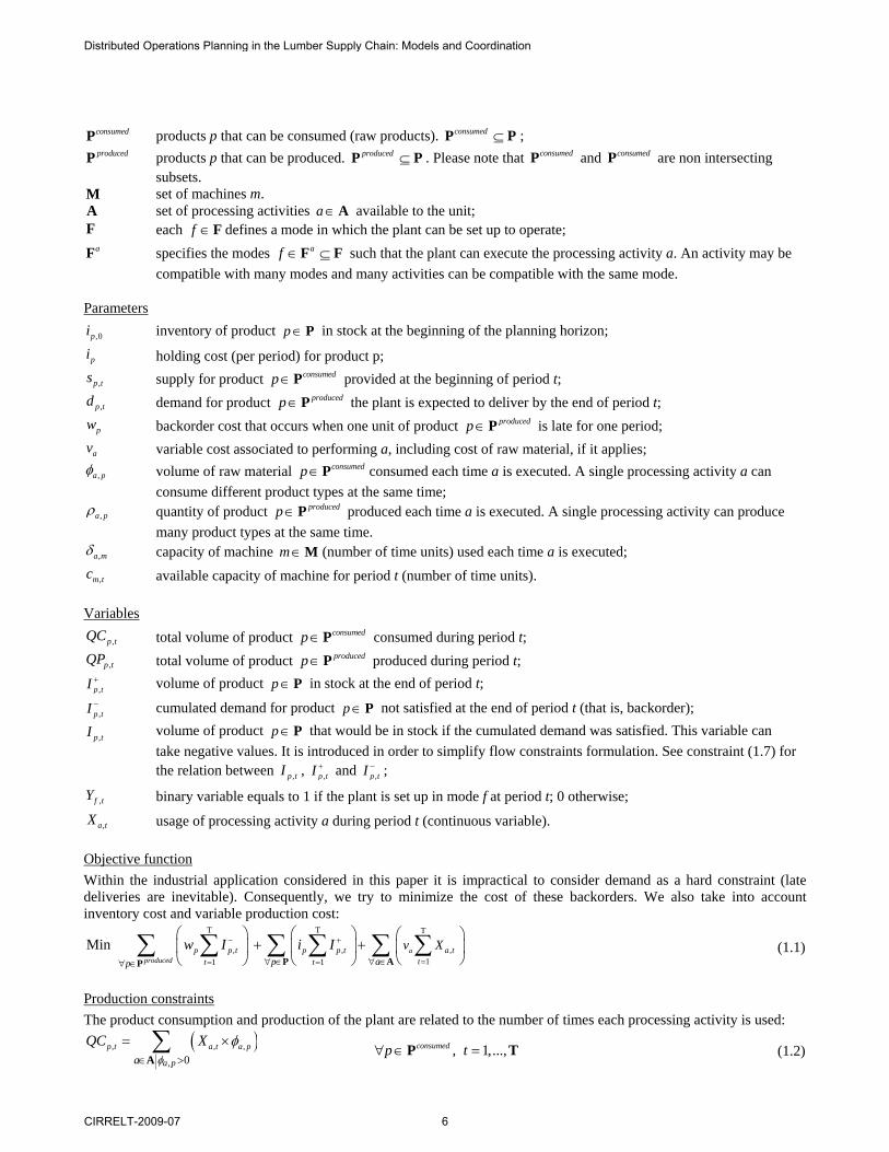
consumedP products p that can be consumed (raw products). consumed ⊆P P ; producedP products p that can be produced. produced ⊆P P . Please note that consumedP and consumedP are non intersecting

subsets. M set of machines m. A set of processing activities a∈A available to the unit; F each f ∈F defines a mode in which the plant can be set up to operate;

aF specifies the modes af ∈ ⊆F F such that the plant can execute the processing activity a. An activity may be compatible with many modes and many activities can be compatible with the same mode.

Parameters

,0pi inventory of product p∈P in stock at the beginning of the planning horizon;

pi holding cost (per period) for product p;

,p ts supply for product consumedp∈P provided at the beginning of period t;

,p td demand for product producedp∈P the plant is expected to deliver by the end of period t;

pw backorder cost that occurs when one unit of product producedp∈P is late for one period;

av variable cost associated to performing a, including cost of raw material, if it applies;

,a pφ volume of raw material consumedp∈P consumed each time a is executed. A single processing activity a can consume different product types at the same time;

,a pρ quantity of product producedp∈P produced each time a is executed. A single processing activity can produce many product types at the same time.

,a mδ capacity of machine m∈M (number of time units) used each time a is executed;

,m tc available capacity of machine for period t (number of time units).

Variables

,p tQC total volume of product consumedp∈P consumed during period t;

,p tQP total volume of product producedp∈P produced during period t;

,p tI + volume of product p∈P in stock at the end of period t;

,p tI − cumulated demand for product p∈P not satisfied at the end of period t (that is, backorder);

,p tI volume of product p∈P that would be in stock if the cumulated demand was satisfied. This variable can take negative values. It is introduced in order to simplify flow constraints formulation. See constraint (1.7) for the relation between ,p tI , ,p tI + and ,p tI − ;

,f tY binary variable equals to 1 if the plant is set up in mode f at period t; 0 otherwise;

,a tX usage of processing activity a during period t (continuous variable).

Objective function Within the industrial application considered in this paper it is impractical to consider demand as a hard constraint (late deliveries are inevitable). Consequently, we try to minimize the cost of these backorders. We also take into account inventory cost and variable production cost:

T T T

, , ,11 1

Min aproduced

p p t p p t a ttt tp ap

v Xw I i I− +

== =∀ ∈ ∀ ∈∀ ∈

⎛ ⎞ ⎛ ⎞ ⎛ ⎞+ +⎜ ⎟ ⎜ ⎟ ⎜ ⎟

⎝ ⎠⎝ ⎠ ⎝ ⎠∑∑ ∑ ∑ ∑ ∑

P AP

(1.1)

Production constraints The product consumption and production of the plant are related to the number of times each processing activity is used:

( ), , ,

, 0p t a t a p

a paQC X

φφ

∈ >

= ×∑A

, 1,...,consumedp t∀ ∈ =P T (1.2)


CIRRELT-2009-07 6

( ), ,,, 0

a t a pp ta pa

QP Xρ

ρ∈ >

= ×∑A

, 1,...,producedp t∀ ∈ =P T (1.3)

At each period t of the planning horizon, the sawing line can be set up in only one mode and thus can only use the processing activities compatible with that mode:

, 1f tf

Y∈

≤∑F

1,...,t∀ = T (1.4)

, ,0a

a t f tf

X Y∈

⎛ ⎞⎜ ⎟≤ ≤ ∞×⎜ ⎟⎝ ⎠

∑F

, 1,...,a t∀ ∈ =A T (1.5)

where ∞ is a significantly large number

The number of times each processing activity is executed is constrained by the capacity of each machine: ( ), , ,a t a m m t

a

X cδ∈

× ≤∑A

, 1,...,m t∀ ∈ =M T (1.6)

Flow constraints Constraint (1.7) and (1.8) together with the objective function allow the computation of backorder level. Of course, no backorder is allowed for raw products (1.9).

, , ,p t p t p tI I I+ −= − , 1,...,Tp t∀ ∈ =P (1.7)

, ,0; 0p t p tI I+ −≥ ≥ , 1,...,Tp t∀ ∈ =P (1.8)

, 0;p tI − = , 1,...,Tconsumedp t∀ ∈ =P (1.9)

Constraints (1.10) and (1.11) establish the relation between inventory, supply and consumption of logs. ,1 ,0 ,1 ,1p p p pI i s QC= + − consumedp∀ ∈P (1.10)

, , 1 , ,p t p t p t p tI I s QC−= + − , 2,...,Tconsumedp t∀ ∈ =P (1.11)

Constraints (1.12) and (1.13) establish the relation between inventory, demand and production. ,1 ,0 ,1p p pI i d= − producedp∀ ∈P (1.12)

, , 1 , 1 ,p t p t p t p tI I QP d− −= + − , 2,...,Tproducedp t∀ ∈ =P (1.13)

Model implementation and resolution For real industrial problems, this model was easily solved using the MIP solver ILOG CPLEX 9.1. Near optimal solutions can be found in a few minutes.

4.1.2 Drying Model

Drying is a multi-stage process (see Section 2.1.2). In the proposed model we chose not to model directly the alternative combination of activities (paths in Figure 4). Instead, we modeled the individual activities. The connection between the activities (i.e. a valid precedence relationship between two activities) is enforced by the stocks level constraints for intermediary products (an intermediary product needed by an activity, must first be produced by its predecessor).

Figure 6 presents the main idea involved in this model. We have different activity types a∈A . Each type of activity can be executed on a compatible machine am∈ ⊆M M , and has a specified duration aδ . The parameters ,a pφ and ,a pρ specify the consumption and production for products p∈P . In this context, building a plan can be seen as deciding which activities to perform, when to do them and which machines to use. A solution can be represented by a Gantt chart of activities (see Figure 6). Each type of activity can be inserted as many times as needed in the plan. Inserted activities have an impact on product inventories ( ),p tI by increasing or decreasing it since they produce and consume different products.

Demand from the finishing unit ( ),p td also influences product inventories. These kinds of models are referred to as a timetable models or time-line models (Bartak, 1999a; 1999b; 2002).


CIRRELT-2009-07 7

Figure 6. Illustration of the drying model

Sets This drying model uses notation similar to the sawing model. The following sets have the same meaning in both models: periods ( )T , products ( )consumed producedP, P , P and machines ( )M . Because drying processes allow intermediary products

which can be both produced and consumed, consumedP and producedP may now intersect. Consequently, in order to simplify the presentation of flow constraints, we will consider each product p∈P as a resource that can be consumed, produced, supplied and shipped.

The following defines other sets used by the drying model: A set of all types of drying activities a;

consumepA subset of activities which consume the product p. consume

p ⊆A A ; producepA subset of activities which produce the product p. produce

p ⊆A A ;

mA subset containing all types of activities that can be processed on machine m∈M . m ⊆A A ;

aM subset of machines that can carry out activity a. { }a mm a= ∈ ∈M M A .

Parameters The following parameters have the same meaning as in the sawing model although they are now defined for every product p∈P : supply ( ),p ts , demand ( ),p td , initial inventory and costs ( ),0 , ,p p pi i w , material consumption and

production of activities ( ), ,,a p a pφ ρ . However, we will suppose that ,p td is equal to zero for all products that can be

consumed. The parameter av also has the same meaning as in the sawing model. In addition, we define these parameters:

,m tc 1, if machine m is available during period t, 0 otherwise;

aδ number of consecutive periods needed to realize activity a.

Variables The following variables have the same meaning as in the sawing model although they are now defined for every product p∈P : ,p tQC , ,p tQP , ,p tI + , ,p tI − , ,p tI . In addition, we define this decision variable:

( , ), a m tX Binary decision variable taking value 1 if an activity of type a starts on machine m at period t, 0 otherwise. It is defined for each couple ( , ) | ma m a∈A .


CIRRELT-2009-07 8

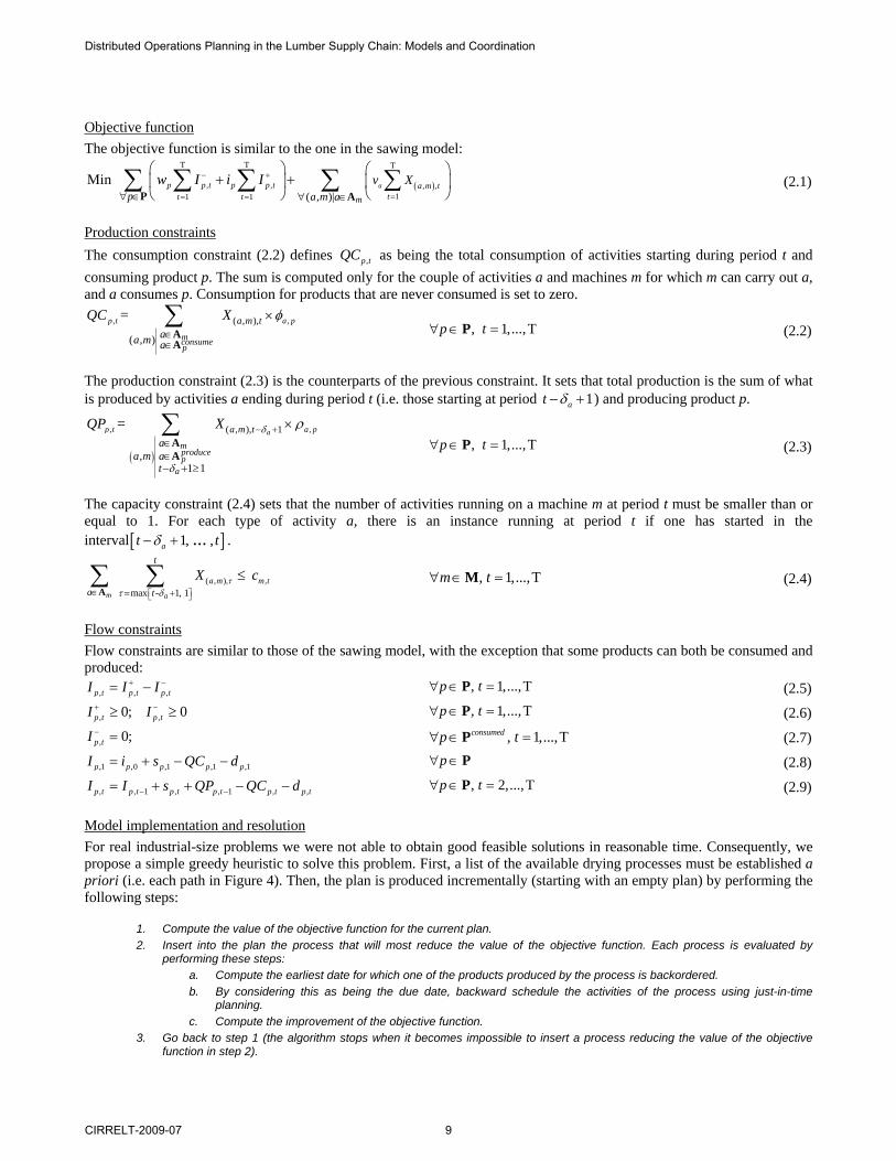
Objective function The objective function is similar to the one in the sawing model:

( )

T T T

, , , ,11 1 ( , )|

Min ap p t p p t a m ttt t mp a m a

v Xw I i I− +

== =∀ ∈ ∀ ∈

⎛ ⎞ ⎛ ⎞+ +⎜ ⎟ ⎜ ⎟

⎝ ⎠⎝ ⎠∑∑ ∑ ∑ ∑

P A (2.1)

Production constraints The consumption constraint (2.2) defines ,p tQC as being the total consumption of activities starting during period t and consuming product p. The sum is computed only for the couple of activities a and machines m for which m can carry out a, and a consumes p. Consumption for products that are never consumed is set to zero.

, ,

( , ),

( , )

=p t a p

mconsumep

a m taa m a

QC X φ∈∈

×∑AA

, 1,...,Tp t∀ ∈ =P (2.2)

The production constraint (2.3) is the counterparts of the previous constraint. It sets that total production is the sum of what is produced by activities a ending during period t (i.e. those starting at period 1at δ− + ) and producing product p.

( )

, ,( , ), 1

,1 1

= ap t a p

mproducep

a

a m ta

a m at

QP X δ

δ

ρ− +∈∈− + ≥

×∑AA

, 1,...,Tp t∀ ∈ =P (2.3)

The capacity constraint (2.4) sets that the number of activities running on a machine m at period t must be smaller than or equal to 1. For each type of activity a, there is an instance running at period t if one has started in the interval [ ]1, ,...at tδ− + .

( , ), ,max - 1, 1m a

a m m t

t

a t

X cττ δ⎡ ⎤⎣ ⎦∈ = +

≤∑ ∑A

, 1,...,Tm t∀ ∈ =M (2.4)

Flow constraints Flow constraints are similar to those of the sawing model, with the exception that some products can both be consumed and produced:

, , ,p t p t p tI I I+ −= − , 1,...,Tp t∀ ∈ =P (2.5)

, ,0; 0p t p tI I+ −≥ ≥ , 1,...,Tp t∀ ∈ =P (2.6)

, 0;p tI − = , 1,...,Tconsumedp t∀ ∈ =P (2.7)

,1 ,0 ,1 ,1 ,1p p p p pI i s QC d= + − − p∀ ∈P (2.8)

, , 1 , , 1 , ,p t p t p t p t p t p tI I s QP QC d− −= + + − − , 2,...,Tp t∀ ∈ =P (2.9)

Model implementation and resolution For real industrial-size problems we were not able to obtain good feasible solutions in reasonable time. Consequently, we propose a simple greedy heuristic to solve this problem. First, a list of the available drying processes must be established a priori (i.e. each path in Figure 4). Then, the plan is produced incrementally (starting with an empty plan) by performing the following steps:

1. Compute the value of the objective function for the current plan. 2. Insert into the plan the process that will most reduce the value of the objective function. Each process is evaluated by

performing these steps: a. Compute the earliest date for which one of the products produced by the process is backordered. b. By considering this as being the due date, backward schedule the activities of the process using just-in-time

planning. c. Compute the improvement of the objective function.

3. Go back to step 1 (the algorithm stops when it becomes impossible to insert a process reducing the value of the objective function in step 2).


CIRRELT-2009-07 9

4.1.3 Finishing Model

In practice, the three steps of the finishing process (i.e., planing, sorting and trimming) are performed on a single production line. For planning purposes, this line can be considered as a single machine, whose production rate is equal to that of the machine which is the bottleneck on the line.

As stated in Section 2.1.3, a finishing production plan is a sequence of campaigns (see Figure 5). Each one has a product family associated to it (e.g. 2”x4”), which is related to a specific setup for the plant. During the campaign, different types of products corresponding to the family can be processed (e.g. 2”x4”-8’, 2”x4”-10’). However, they must be processed in a specific order.

It the following model, binary decision variables specify how the plant is setup at each period. A setup cost ( )ζ must be accounted each time there are two consecutive periods with a different setup (that is, each time a new campaign begins). Other decision variables in the model represent the quantities of each length (e.g. 8’, 10’) to process at each period (rather than the quantity to process at each campaign as imposed by the problem). To compensate for this “relaxation”, a constraint states that all the consumption of the campaign takes place at its beginning, and its production at the end. On the other hand, we have to maintain two different inventories: one in the yard (similar to the sawing and drying problems) and one in the plant.

Sets This finishing model uses notation similar to previous models. The following sets have the same meaning: T , P , consumedP , and producedP . Similar to the sawing model, each f ∈F defines a mode in which the plant can be set up to operate. Each mode corresponds to a product family (e.g. 2″x4″). In addition, we define the following sets:

consumedfP products p that can be consumed when the plant is set up in mode f. consumed consumed

fp∈ ⊆P P ; producedfP finished products p that can be produced when the plant is set up in mode f. produced produced

fp∈ ⊆P P ; FP set of couples ( ) ( ) ( ), consumed

ff p f p∈ ∧ ∈F P .

Parameters The following parameters have the same meaning as in the sawing model: ,p ts , ,p td , ,0pi , pi , and pw . In addition, we define these parameters:

( ), ' ,f p pρ volume of product producedp∈P produced when one unit of product ' consumedp ∈P is consumed while the plant is set up in mode f. Defined for couples ( ), 'f p ∈FP ;

( ),f pδ time needed to consume one unit of product consumedp∈P when the plant is set up in mode f. Defined for couples ( ),f p ∈FP ;

( ),f pv cost of processing one unit of product consumedp∈P . Defined for couples ( ),f r ∈FP ;

tc capacity of the plant (number of time unit) for period t; ζ cost of performing a setup change.

Variables The following variables have the same meaning as in the sawing model. Variable ,f tY identify in which mode the plan is set

up. The variables ,p tI + , ,p tI − and ,p tI corresponds to the inventory in the yard. Variable ,p tQC corresponds to a quantity transferred in the plant at the beginning of a campaign. Variable ,p tQP to a quantity transferred from the plant to the yard at the end of the campaign.

In addition, we define these variables: ,f tBS 1, if the plant is set up for mode f at period t and it was not the case at period t-1. 0, otherwise. Said

otherwise, this variable is equal to 1 if a campaign using mode f begins at period t; tBS 1, if a campaign (of any mode) begins at period t. 0, otherwise;

tBE 1, if a campaign (of any mode) ends at period t. 0, otherwise.

( ), ,f p tUC volume of raw product p to process at period t while the plant is set up in mode f. The product must be already in the plant to be processed. Defined for couples ( ),f p ∈FP .


CIRRELT-2009-07 10

,p tUP volume of product p produced at period t. The product remains in the plant and is not available to satisfy demand until the end of the campaign. It will be released and thus be considered a production of the plant only when the campaign is over. Defined for producedp∈P ;

,p tUI volume of product p in the plant at the end of period t. Defined for p∈P .

Objective function The objective function is similar to the one in the sawing model although in this problem the setup costs are taken into account. Production costs depend both on how the plant is set up and the raw material consumed.

( ) ( )( )

T T T T

, , , ' , ' ,1 11 1 , '

Min produced

tp p t p p t f p f p tp t tt tp f p

BS v UCw I i I ζ− +

∀ ∈ = == =∀ ∈ ∀ ∈

⎛ ⎞ ⎛ ⎞ ⎛ ⎞+ + +⎜ ⎟ ⎜ ⎟ ⎜ ⎟

⎝ ⎠⎝ ⎠ ⎝ ⎠∑ ∑∑ ∑ ∑ ∑ ∑

P P FP (3.1)

Production constraints First, the plant can only be set up in one mode at a time (3.2) and a product can be processed (consumed) only if the plant is configured in a compatible mode (3.3).

, 1f tf

Y∈

≤∑F

1,...,Tt∀ = (3.2)

( ) ( ),, ,0 f tf p tUC Y≤ ≤ ∞ ( ), , 1,...,Tf p t∀ ∈ =FP (3.3)where ∞ is a significantly large number.

Constraints (3.4) to (3.6) state a batch can start or end only if the plant is set up in a compatible mode. Constraint (3.7) ensures that a specific batch will run until it has ended.

,1 ,1f fBS Y= f∀ ∈F (3.4)

, ,f t f tBS Y≤ , 1,...,Tf t∀ ∈ =F (3.5)

, ,f t f tBE Y≤ , 1,...,Tf t∀ ∈ =F (3.6)

, , 1 , 1 ,f t f t f t f tY Y BE BS− −= − + , 2,...,Tf t∀ ∈ =F (3.7)

Variables tBS and tBE respectively take value 1 if and only if a batch is starting (3.8) or ending (3.9) at period t.

,t f tf

BS BS∈

=∑F

1,...,Tt∀ = (3.8)

,t f tf

BE BE∈

=∑F

1,...,Tt∀ = (3.9)

Raw products can enter the plant only at the beginning of a compatible campaign (3.10). Finished products are released only at the end of the campaign (3.11). No products can be left inside the plant at the end of the campaign (3.12).

, ,consumedf

p t f tf p

QC BS∈ ∈

⎛ ⎞⎜ ⎟≤ ∞⎜ ⎟⎝ ⎠

∑F P

, 1,...,Tp t∀ ∈ =P (3.10)

, ,producedf

p t f t

f p

QP BE∈ ∈

⎛ ⎞⎜ ⎟≤ ∞⎜ ⎟⎜ ⎟⎝ ⎠

∑F P

, 1,...,Tp t∀ ∈ =P (3.11)

( ), 1p t tUI BE≤ ∞ − , 1,...,Tp t∀ ∈ =P (3.12)

The following are the flow conservation constraints for the raw products inside the plant:

( )( )( )

,1 ,1 , ,1,

p p f pf F f p

UI QC UC∈ ∈

= − ∑FP

consumedp∀ ∈P (3.13)

( )( )( )

, , 1 , , ,,

p t p t p t f p tf F f p

UI UI QC UC−∈ ∈

= + − ∑FP

, 1,...,Tconsumedp t∀ ∈ =P (3.14)

, 0p tUI ≥ , 1,...,Tconsumedp t∀ ∈ =P (3.15)


CIRRELT-2009-07 11

These are the flow conservation constraints for the finished products inside the plant: ,1 ,1 ,1p p pUI UP QP= − producedp∀ ∈P (3.16)

, , 1 , ,p t p t p t p tUI UI UP QP−= + − , 2,...,Tproducedp t∀ ∈ =P (3.17)

, 0p tUI ≥ , 1,...,Tconsumedp t∀ ∈ =P (3.18)

These constraints establish the relation between consumption and production inside the plant:

( ) ( )( )

, , ' , , ' ,, '

p t f p t f p pf p

UP UC ρ∈

= ×∑FP

, 1,...,Tp t∀ ∈ =P (3.19)

Finally, the capacity of the finishing line must be respected:

( ) ( )( )( )

, , ,,

tf p t f pf p

UC cδ∈

× ≤∑FP

1,...,Tt∀ = (3.20)

Flow constraints (yard) The constraints for the product flow in the yard are the same as in the sawing model. Therefore, we reuse constraints (1.7) to (1.13) in order to establish the relations between ,0pi , ,p tI , ,p tI + , ,p tI − , ,1ps , ,p td , ,1pQC and ,p tQP .

Model implementation and resolution As for the drying model, we were not able to obtain good feasible solutions in reasonable time for real industrial problems. Again, we proposed a simple greedy heuristic to solve this problem. Each time the finishing line is available, we start a campaign for the product family f ∈F for which it is most urgent to start production (i.e. the family with the smallest “first period with unsatisfied orders minus expected production time”). Because of setup costs, we want this campaign to have the longest possible duration (i.e. satisfying as many future orders as possible). However, the campaign must be over before the next delivery date. We also need to leave room for the production of other families. Here is the detailed pseudocode:

1. Let t be the first period for which the finishing line and some raw material are available.

2. For each mode f ∈F :

a. Let ft be the first period where an order for a product producedfp∈P is not satisfied according to the current

production plan.

b. Let us suppose a campaign ending at 1t fe t= − that allows satisfying the demand for all producedfp∈P at period

ft (without considering raw material availability). Let fs be the start time of this campaign according to the

needed production duration.

c. If there is no raw material consumedfp∈P available at fs , increase fs until some is ( fe remains unchanged).

3. Sort the modes f in increasing order of fs .

4. Considering the modes f ∈F for which we have some raw material consumedfp∈P available at period t , select the one

with the smallest fs . Insert a campaign for this mode into the plan:

a. It begins at t .

b. It has the longest possible duration (according to raw material availability) but without trespassing ft (next

delivery date for current family) or the next fs in the vector of step 3 (starting date of a campaign for the next most

urgent family). c. The consumed products/quantities are established as follows:

i. Quantifies of producedfp∈P needed to satisfy the next unsatisfied order for this family.

ii. If room is available, the quantities for the next order of this family, etc. 5. Go back to step 1.

4.2 Coordination Mechanisms

In a distributed planning system, it is necessary to deploy a coordination mechanism between the different production units in order to integrate the different plans so as to make sure they are coherent with each other (in terms of material


CIRRELT-2009-07 12

availability) but also to guarantee a certain level of collective performance. Such a strategy defines which information is transmitted from one agent to the other, when it is transmitted and what the sequence used to propagate the information is.

The most common class of coordination mechanisms (both in literature and industrial practice) can be described as hierarchical. In this approach there is a sequence (naturally defined or specified in a long-term agreement) specifying the order in which the partners must plan their operations. Schneeweiss (2003) describes many problems using real industrial applications to illustrate the challenge of distributed decision making. In this section, we describe three different coordination mechanisms, which are (1) upstream planning, (2) two-phase planning and (3) bottleneck-first planning. Then, a modification to the last two mechanisms is proposed in order to push alternative products.

4.2.1 Upstream Planning

The most common hierarchical approach is referred to as upstream planning (Bhatnagar et al, 1993; Dudek et al, 2005). Agents plan their operations one after the other, beginning with the agent that is closest to the customer (right-hand side agent in Figure 7). Knowing demand from the external customer, this agent plans its activities. This allows identifying the supply need of the production unit (in the model, its supply parameter ,p ts is transformed into a variable). This supply need

is then transferred to its supplier and becomes demand for the latter ( ),p td . All this presupposes that each agent is always able to satisfy any demand. Of course, this assumption cannot be met in all contexts. This is why it cannot be used in our application and is furthermore not implemented.

Figure 7. Upstream planning

4.2.2 Two-phase Planning

One variant of this approach, particularly relevant in a process industry with strong supply constraints, is to apply two planning phases: one upstream and the other downstream (see Figure 8). This approach involves each agent twice. The agent first makes a temporary plan to compute its supply needs and sends this information to its supplier. In turn, the supplier tries to satisfy this demand and responds with a supply plan that does not necessarily meet all demand (e.g., some deliveries may be planned to be late or some products can be replaced by substitutes). When informed of the supply granted by its supplier, the initial agent has to revise its production plan in order to account for supply constraints. The task flow forms a loop with two phases: one upstream where demand is tentatively propagated and the other downstream where final supply is propagated.

Figure 8. Two-phase planning

4.2.3 Bottleneck-first Planning

A truncated version of the two-phase planning approach is illustrated in Figure 9. The external customer demand is transmitted directly to the drying agent instead of going through the finishing agent. This modification is inspired by the proposition from Goldratt et al (1992) to plan the production bottleneck first. In the lumber supply chain, the drying


CIRRELT-2009-07 13

production center is often the bottleneck because of the investment needed to deploy kiln dryers. Kiln drying duration can span from 12 to 60 hours, immobilizing and having a tremendous impact on the flexibility of the supply chain.

Figure 9. Bottleneck-first planning

Because demand for finished products is transmitted to the drying agent, it must have a definition of the finishing processes. This is done by adding the finishing activities in the graph of activities (Figure 4). By doing so, the drying agent has a simplified representation of the finishing unit processes.

4.2.4 Pushing alternative products

In our context, internal demand (demand from one unit to another) cannot be considered as a hard constraint. When a production unit cannot satisfy all the demand of a partner, it might be useful to propose alternative products to this partner. With this option in mind, a simple modification to the previous mechanisms (two-phase and bottleneck-first) is proposed.

In the downstream phase, the unit uses available production capacity to produce alternative products and “push” them to the next unit (hoping it will be able to use them). To do this, we simply run the planning model of the agent another time: we remove the already used capacity and raw material, and provide the model high demand for other products. In the objective function, these products are weighted ( )pw using their respective expected market value.

5. INDUSTRIAL APPLICATION

This section presents work that was done with an industrial partner in order to validate the models (Section 5.1). We then show how an agent-based simulation platform was used in order to study the impact of different coordination mechanisms. The planning models were embedded in an agent-based platform (Section 5.2) and simulations were done in order to evaluate the coordination mechanisms according to the supply chain performance (Section 5.3). Finally, Section 5.4 discusses related work.

5.1 Process Modeling and Industrial Validation

In order to carry out validation of the proposed planning models, we developed a case study with a lumber company which includes production processes, products, orders, on-hand inventory, selling prices, resource costs, forecasted supply, capacity and work-in-process inventories. Processes were modeled in collaboration with the company’s production manager. Customer data and on-hand inventory data were extracted from the partner’s ERP system. Finally, the partner’s sales team provided the data about product prices and resource costs.

Each planning model was assessed using real industrial data in an off-line planning mode. Each week, the partner’s production manager sent us updated production data, which we used to generate a production plan. The production manager gave feedback concerning the quality and feasibility of the plans. This interactive validation phase allowed us to review and adjust the planning parameters as well as the planning models. This validation process took about one year and many corrections were made to the models.

5.2 Agent-based Planning Platform

In order to develop an Advanced Planning and Scheduling (APS) system for the lumber supply chain, the FORAC Research Consortium of Université Laval (Québec, Canada) has developed an agent-based planning platform. In brief, this platform aims to address: (1) the ability to plan and coordinate operations throughout the supply chain; and (2) the ability to analyze the dynamics and simulate different supply chain scenarios through simulation. It allows the user, whether a production manager or a researcher, to evaluate and compare different planning models, coordination mechanisms or supply chain


CIRRELT-2009-07 14

configurations, according to user specified performance measures. Essentially, each planning model is embedded within a software agent that has the capacity to manipulate data, solve its planning model, and exchange information with other agents according to coordination mechanisms. To allow specification of coordination mechanisms, the platform relies on the concepts of conversation protocols that are commonly used in multi-agent systems. The interested reader is referred to Frayret et al (2007) for a more thorough description of the design specifications and functions of this platform.

5.3 Simulation

We simulated the coordination mechanism using the agent-based planning platform described previously. A virtual supply chain was built, based on the industrial case. The planning agents (i.e., sawing, drying and finishing) were set up according to these data. The studied case has a total of 393 types of production activities and 114 products, including 45 finished products available to the external customer. Orders were generated using a probabilistic demand generator (Lemieux et al, 2008), for a 50-day planning horizon. This generator created random demand, according to predetermined settings such as distribution functions, minimum/maximum limits and seasonality as well. However, we did not simulate the replenishment of the sawing unit; we considered unlimited log supply.

Table 1 presents the performance of four coordination mechanisms (two-phase planning and bottleneck-first; with or without the option of pushing alternative products). The performance indicators used to compare the mechanisms are: (a) the percentage of late deliveries, (b) the average tardiness for late deliveries and (c) the average tardiness per ordered unit (that is, “a” multiplied by “b”).

Results show a clear advantage to bottleneck-first planning over two-phase planning. This is due to the advantage of planning production of the bottleneck (here the drying agent) first, which sets the total capacity of the entire supply chain. Also, pushing alternative products allowed an additional reduction of backorders for both coordination mechanisms. The hybrid approach of bottleneck-first planning with the ability to push alternative products gave the best results in this case.

Two-phase planning Bottleneck-first planning Satisfy demand Satisfy demand

+push alt. products Satisfy demand Satisfy demand +push alt. products

Late deliveries (%) 49.94 % 28.27 % 44.18 % 26.20 %

Average tardiness (days) per late unit volume delivered 4.58 1.74 0.95 0.16

Average tardiness (days) per unit volume ordered 2.29 0.49 0.42 0.04

Table 1. Coordination mechanisms evaluation

5.4 Related Work

The previous section showed how such methodology can be used to study the impacts of different coordination mechanisms on a supply chain. However, the results should not be used as generic prescriptions for the lumber industry as they are specific to this case study. The best coordination mechanism to use depends on various factors; moving the bottleneck or changing the mix of alternative products can have a major impact on the performance of the mechanisms.

As an illustration of this, Cid-Yanez et al (To appear) used the platform and the planning model introduced here in order to study the impact of moving upward the point up to where demand information is transmitted (i.e., the decoupling point, called the push-pull limit; beyond that point agent just push products). Nine supply chain configurations were investigated under six different environmental conditions in order to carry out a complete mixed level design of 54 simulation runs. Each of these configurations was a combination of a decoupling point position and a capacity level committed to contracts with customers. Similarly, the environmental conditions were designed as a combination of supply type (i.e., log diameter distribution) and lumber market prices.


CIRRELT-2009-07 15

Figure 10. Studied decoupling point positions

This study demonstrated the advantage in terms of logistic performance of setting up the decoupling point position as far upward as possible. However, this also illustrated the cost of such a practice in terms of total value creation. In other words, setting up the models presented in this paper so as to maximize customer demand satisfaction instead of simply producing the most valuable products at each stage and pushing them downward, has the effect of decreasing the overall value of total production. Consequently, making a commitment to regularly meet a customer’s demand, is a service that must be paid through adding a premium to the market price.

6. CONCLUSION

This paper described the production planning problems and models for three production units in the North American softwood lumber industry. The models can be used individually or in a distributed supply chain context. Different coordination mechanisms have been described. We showed how the planning models can be integrated in an agent-based planning platform in order to evaluate and compare the coordination mechanisms.

Different improvements can be made to the models and coordination mechanisms. For example, an agent could exploit information about partner’s preference regarding alternative products. Also, it might be interesting to use simulation tools to evaluate the robustness of the system in a context where unexpected events happen.

Finally, other coordination mechanisms are studied in order to offer alternatives to the ones presented in this paper. Forget et al (2008) have proposed an intelligent planning agent model, called multi-behavior agent, which can adapt its coordination mechanisms according to specific states in its environment. Also, Gaudreault et al (To appear) have proposed a distributed planning algorithm based on distributed constraint optimization, where agents are requested to submit multiple local plans in order for the collective to find the best arrangements of plans.

7. REFERENCES

1. Bartak, R. (1999a). Conceptual Models for Combined Planning and Scheduling. Proceedings of the CP99 Workshop on Large Scale Combinatorial Optimization and Constraints. Alexandria, USA, pp. 2-14.

2. Bartak, R. (1999b). On the Boundary of Planning and Scheduling: A Study. Proceedings of the Eighteenth Workshop of the UK Planning and Scheduling Special Interest Group (PlanSIG), Manchester, UK, pp. 28-39.

3. Bartak, R. (2002). Visopt ShopFloor: on the edge of planning and scheduling. Proceedings of the Principles and Practice of Constraint Programming International Conference, LNCS#2470, Ithaca, USA, pp. 587-602.

4. Bhatnagar, R., Chandra, P. and Goyal, S.K. (1993). Models for multi-plant coordination. European Journal of Operational Research, 67(2): 141-160.

5. Cid-Yanez, F., Frayret J.M., Leger, F. and Rousseau, A. Agent-Based Simulation and Analysis of Demand-driven


CIRRELT-2009-07 16

Production Strategies in the Lumber Industry. International Journal of Production Research (To appear). 6. Dudek, G. and Stadtler, H. (2005). Negotiation-based collaborative planning between supply chains partners.

European Journal of Operational Research, 163(3): 668-687. 7. Feng, Y., D'Amours, S. and Beauregard, R. (2008). The value of Sales and Operations Planning in Oriented Strand

Board Industry with Make-to-Order Manufacturing System: Cross functional integration under deterministic demand and spot market recourse. International Journal of Production Economics, 115: 189-209.

8. Forget, P., D’Amours, S. and Frayret, J. M. (2008). Multi-Behavior Agent Model for Planning in Supply Chains: An Application to the Lumber Industry. Robotics and Computer-Integrated Manufacturing, 24: 664-679.

9. Frayret, J.M. (2002). A conceptual framework to operate collaborative manufacturing networks. Ph.D. thesis, Université Laval.

10. Frayret, J.M., D’Amours, S., Rousseau, A., Harvey, S. and Gaudreault, J. (2007). Agent-based Supply Chain Planning in the Forest Products Industry. International Journal of Flexible Manufacturing Systems, 19(4): 358-391.

11. Gaudreault, J., Forget, P., Frayret, J.-M., Rousseau, A., D’Amours, S., 2008. A multi-agent and OR-based approach to operations planning in the lumber industry, 13th Annual International Conference on Industrial Engineering Theory, Applications & Practice, September 7- 10, Las Vegas, Nevada.

12- Gaudreault, J., Frayret, J.M., Pesant, G. Distributed Search for Supply Chain Coordination, Computers in Industry, Part 2 of the Special Issue on Advances in Collaborative Engineering, from Concurrent Engineering to Collaborative Manufacturing (To appear).

13. Goldratt, E.M. and Cox, J. (1992). The goal: a process of ongoing improvement. North River Press, New York, USA. 14. Lemieux, S., D'Amours, S., Gaudreault, J. and Frayret, J.M. (2008). Intégration d'outils APS dans une simulation

multi-agent. Proceedings of the MOSIM’08 Conference, Paris, France, pp. 1037-1045. 15. Maness, T.C. and Adams, D.M. (1993). The combined optimization of log bucking and sawing strategies. Wood and

Fiber Science, 23(2): 296–314. 16. Maness, T.C. and Norton, S. E. (2002). Multiple period combined optimization approach to forest production

planning. Scandinavian Journal of Forest Research, 17(5): 460-471. 17. Maturana, F., Shen, W. and Norrie, D.H. (1999). MetaMorph: an adaptive agent-based architecture for intelligent

manufacturing. International Journal of Production Research, 37(10): 2159-2173. 18. Ouhimmou, M., D’Amours, S., Beauregard, R., Ait-Kadi, D. and Singh, C.S. (2008). Furniture supply chain tactical

planning optimization using a time decomposition approach. European Journal of Operational Research, 189: 952-970.

19. Schneeweiss, C. (2003). Distributed Decision Making. Springer, New York, USA. 20. Singer, M. and Donoso, P. (2007). Internal supply chain management in the Chilean sawmill industry. International

Journal of Operations and Production Management, 27(5): 524-541. 21. Stadtler, H. (2005). Supply chain management and advanced planning - basics, overview and challenges. European

Journal of Operational Research, 163(3): 575-588. 22. Stadtler, H. and Kilger, C. (2005). Supply Chain Management and Advanced Planning. Springer, New York, USA. 23. Strader, T.J., Lin, F. R. and Shaw, M.J. (1998). Simulation of Order Fulfillment in Divergent Assembly Supply

Chains. Journal of Artificial Societies and Social Simulation, 1(2). 24. Thomas, D.J., and Griffin, P.M. (1996). Coordinated supply chain management. European Journal of Operational

Research, 94(1): 1-15.


CIRRELT-2009-07 17

distributed operations planning in the lumber …distributed operations planning in the lumber...

Documents