distributed monitoring of concurrent and asynchronous … · partners of the project are france...

Distributed Monitoring of Concurrent andAsynchronous Systems*

ERIC FABRE

Campus de Beaulieu, IRISA/INRIA, 35042, Rennes Cedex, France

ALBERT BENVENISTE. [email protected]


STEFAN HAAR


CLAUDE JARD

Campus de Ker-Lann, IRISA/ENS-Cachan, 35170, Bruz, France

Abstract. In this paper we study the diagnosis of distributed asynchronous systems with concurrency.

Diagnosis is performed by a peer-to-peer distributed architecture of supervisors. Our approach relies on Petri

net unfoldings and event structures, as means to manipulate trajectories of systems with concurrency. This

article is an extended version of the paper with same title, which appeared as a plenary address in the

Proceedings of CONCUR’2003.

Keywords: asynchronous, concurrent, distributed, unfoldings, event structures, fault diagnosis, fault

management

1. Introduction

In this paper we consider fault diagnosis of distributed and asynchronous Discrete Event

Systems (DES). The type of system we consider is depicted in Figure 1. It consists of a

distributed architecture in which each supervisor is in charge of its own domain, and the

different supervisors cooperate at constructing a set of coherent local views for their

respective domains. Each domain is a networked system, in which alarms are collected

and processed locally by the supervisor (shown as a larger gray circle). The different

domains are interconnected by a network, represented by the BIP-cloud.^ The situation is

summarized as follows:

REQUIREMENTS 1

1. The overall system is composed of several subsystems. Each subsystem has its own

supervisor.

Discrete Event Dynamic Systems: Theory and Applications, 15, 33–84, 2005# 2005 Springer Science + Business Media, Inc. Manufactured in The Netherlands.

* This work was supported by the RNRT project MAGDA2, funded by the Ministere de la Recherche; other

partners of the project are France Telecom R&D, Alcatel, Ilog, and Paris-Nord University.

. Corresponding author.

2. The communications between the subsystems, and within each subsystem, are

asynchronous.

3. Each supervisor has knowledge of the local model of its subsystem, together with

relevant information regarding the interface with adjacent subsystems.

4. Each supervisor collects data from sensors that are local to its subsystem. Sensors

from different sites are not synchronized.

5. The duty of each supervisor is to construct a B local projection^ of the global

diagnosis, for the overall system.

6. To this end, the different supervisors act as peers, by exchanging information,

asynchronously, with the other supervisors.

The above requirements were motivated by our application to distributed fault man-

agement in telecommunications networks and services (Aghasaryan et al., 2002, 2004;

Fabre et al., 2004a, 2004b). Since faults in this context are typically transient, providing

explanations in the form of Bcorrelation scenarios^ showing the causal relations between

faults and alarms, is essential. Therefore, we concentrate on constructing such scenarios,

leaving aside the additional questions of fault isolation and diagnosability.

To serve as a background for the reader, here are some figures that are borrowed from

our realistic example reported in (Fabre et al., 2004a): each subsystem is an

asynchronous network of automata, each automaton has a handful of states, and there

are from hundreds to thousands of such automata in the network. Each root fault can

cause hundreds of correlated alarms that travel throughout each subsystem and are

collected by the corresponding local supervisor. Supervised domains may very well be

orders of magnitude larger in the future. Thus, scalability is a major concern. It is

important that the type of algorithm we develop takes this context into account. Never

Figure 1. Three domains with cooperating supervisors.

34 FABRE ET AL.

constructing the overall diagnoses but rather only their local projections, ensures

scalability, from subsystems to the overall system. This motivated Requirement 1.5.

In this paper, we address the problem of distributed monitoring of DES according to

Requirements 1. Our approach has the following features:

� We follow a model-based approach, that is, our algorithms use a model of the underlying

system. In this direction, the diagnoser approach by Lafortune et al. (Sampath et al.,

1995, 1996) is a very elegant technique that consists in Bpre-computing^ all possible

diagnoses, for each possible history of events, in the form of an enriched observer of the

system for monitoring. Diagnosers provide the fastest on-line algorithms for diagnosis,

at the price of excessive memory requirements. Given our context, we do not adopt this

approach. We follow instead a more Binterpreted^ approach, in which the set of all

possible Bcorrelation scenarios^ relating hidden faults and the observed alarms are

computed, on-line. Thus, we trade off speed for memory. The closest approach to ours

we know of in this respect is that of Lamperti and Zanella (2003).

� An asynchronous network of automata can be seen and handled as a single automaton.

However, the resulting automaton has an infinite number of states unless we assume

bounded buffering of the communications. Even so, its size is exponentially larger

than its components and becomes quickly unacceptable. An important source of

reduction in the size of the objects handled consists in taking advantage of the

concurrency that is typically exhibited between the different components. To this end,

in a given history of the system, events that are not causally related are simply not

ordered. Thus, a history is a partial order of events.

� Histories can share prefixes. To reduce the data structures handled by the algorithms,

it is desirable to represent shared prefixes only once. Unfoldings and event structures

were concepts introduced in the early eighties by Winskel (1982) for this purpose. An

impressive theoretical apparatus has been developed since then (Winskel, 1985, 1987)

to provide proper notions of parallel composition, based on tools from category

theory. Our algorithms represent both the system for supervision, and the Bcorrelation

scenarios^ relating faults and alarms, by means of unfoldings and event structures.

The mathematical framework that comes with this was essential in formally proving

our algorithms.

Less importantly, we use safe Petri nets to model asynchronous systems with

concurrency. Executions of safe Petri nets are naturally represented by means of

unfoldings or event structures.

� In the algorithms we develop, the different supervisors act as peers, with no overall

synchronization or scheduling. They read local alarms, receive messages from and

send messages to other peers, using fully asynchronous communications.

� Limitations of our approach are the following:

Y We do not address fault tolerance, i.e., the loss of alarms or communication

messages between peers. This extension is a mild one, however.

DISTRIBUTED MONITORING OF CONCURRENT AND ASYNCHRONOUS SYSTEMS 35

Y We assume that a model of the system is at hand. Given our context, such a model

cannot be constructed by hand. How to construct Bautomatically^ such a model in

the context of telecommunications network and service management, is reported

in (Aghasaryan et al., 2004).

Y We assume that our model is valid. Overcoming this limitation is a more difficult

and less classical problem.

Y Last but not least, we do not address dynamic reconfiguration, i.e., the fact that the

system structure itself is subject to changes. Clearly, this is a needed extension for

our motivating application. Clearly also, pre-compiled approaches such as that of

diagnosers cannot handle this. In contrast, our more Binterpreted^ approach is

better suited at addressing dynamic reconfiguration.

The paper is organized as follows. The problem of distributed diagnosis is extensively

discussed in Section 2, based on a toy example. In particular, we introduce the

architecture of our distributed algorithm and motivate the mathematical apparatus on

event structures that we introduce in Section 3. Using this framework, we formally set

the problem of distributed diagnosis of asynchronous systems in Section 4. To overcome

the sophistication of distributed diagnosis, we structure it into a higher level orchestration

based on a small set of primitive operations on event structures. These primitives are

introduced and studied in Section 5. Then, the orchestration is presented in Section 6, and

the overall algorithms for both off-line and on-line distributed diagnosis are formally

analysed. Finally, related work is discussed in Section 7 and conclusions are drawn.

2. Discussing distributed diagnosis using a toy example

In this study we consider a distributed system with asynchronous communications and

concurrency, both between and within the different subsystems. Several mathematical

frameworks could be considered for this purpose, and indeed used to develop our

approach. We have chosen safe Petri nets as our mathematical framework, for the

following reasons: 1) safe Petri nets are a natural model of systems with local states,

asynchronous communications, and internal concurrency, 2) safe Petri nets can be

composed, 3) unfoldings and event structures have been extensively studied to represent

executions of safe Petri nets with concurrency, and 4) safe Petri nets are a convenient

support for the intuition. In this section, we present and discuss a toy illustrative example

used throughout the paper. Also, we introduce the minimal mathematical framework on

safe Petri nets and their unfoldings that is needed to properly understand this example.

2.1. Prerequisites on safe Petri nets

Basic references are (Cassandras and Lafortune, 1999; Desel and Esparza, 1995; Reisig,

1985). A net is a triple N ¼ ðP; T ;!Þ, where P and T are disjoint sets of places and

transitions, and ! � (P � T ) [ (T � P) is the flow relation. Let and � denote the

reflexive and irreflexive transitive closures of the flow relation !, respectively. Places

36 FABRE ET AL.

and transitions are called nodes, generically denoted by x. For x 2 P [ T, we denote by�x = {y : y! x} the preset of node x, and by x� = {y : x! y} its post-set. For X P [ T,

we write �X = [x2X�x and X � = [x2X x�.

For N a net, a marking of N is a multi-set M of places, i.e., a map M : P 7! {0, 1, 2,

. . . }. A Petri net is a pair P ¼ ðN; M0Þ, where N is a net having finite sets of places and

transitions, and M0 is an initial marking. A transition t 2 T is enabled at marking M if

M( p) 9 0 for every p 2 �t. Such a transition can fire, leading to a new marking M 0 = M

j�t + t�, denoted by M[tiM 0. Petri net P is safe if M(P) � {0, 1} for every reachable

marking M. Throughout this paper, we consider only safe Petri nets, hence marking

M can be regarded as a subset of places.

For N ¼ ðP; T ;!Þ a net, a labeling is a map � : T 7! A, where A is some finite

alphabet. A net N ¼ ðP; T ;!; �Þ equipped with a labeling � is called a labeled net. The

language LP of labeled Petri net P is the subset of A* consisting of the words �(t1) �(t2)

�(t3), . . . , where M0[t1iM1[t2iM2[t3iM3 . . . ranges over the set of finite firing sequences

of P. Note that LP is prefix closed. For N i ¼ fPi; Ti;!i; �ig; i 2 f1; 2g, two labeled

nets, their synchronous product (or simply Bproduct,^ for short) is defined as follows:

N 1 � N 2 ¼def ðP; T ;!; �Þ;where:

P ¼ P1 ] P2; where ] denotes the disjoint union

T ¼ft ¼def

t1 2 T1 j�1ðt1Þ 2 A1 =A2g ðiÞ[ ft ¼def ðt1; t2Þ 2 T1 � T2 j�1ðt1Þ ¼ �2ðt2Þg ðiiÞ[ ft ¼def

t2 2 T2 j�2ðt2Þ 2 A2 =A1g; ðiiiÞ

8><>:

p! t iff

p 2 P1 and p!1 t1 for case (i)

9i 2 f1; 2g : p 2 Pi and p!i ti for case (ii)

p 2 P2 and p!2 t2 for case (iii)

8<:

and t! p is defined symmetrically. In cases (i,iii) only one net fires a transition and this

transition has a private label, while the two nets synchronize on transitions with identical

labels in case (ii). Petri nets and occurrence nets inherit the above notions of labeling and

product.

For N i ¼ fPi; Ti;!ig; i 2 f1; 2g, two nets such that T1 7 T2 = ;, their parallel

composition is the net

N 1 jj N 2 ¼def ðP1 [ P2; T1 [ T2;!1 [ !2Þ: ð1Þ

Petri nets and occurrence nets inherit this notion. For Petri nets, we adopt the convention

that the resulting initial marking is equal to M1,0 [ M2,0, the union of the two initial

markings. Note that any safe Petri net is the parallel composition of its elementary nets

consisting of a single transition together with its pre-set and post-set.

2.2. Presenting the running example, and the problem

Our running example involves two interacting components. Both components can fail,

independently. In addition, the 2nd component uses the services of the 1st one, therefore

it fails delivering its service when the 1st component fails. Alarms reported do not

distinguish between a true failure and a failure to delivery service due to the other

component. Thus, nondeterminism results in the interpretation of alarm messages.


Our example is shown in Figure 2, in the form of a labeled Petri net with two

components interacting via parallel composition (1); these components are numbered 1

and 2. Component 2 uses the services of component 1, and therefore may fail to deliver

its service when component 1 is faulty. The two components interact via their shared

places 3 and 7, represented by the gray zone; note that this Petri net is safe.

Component 1 has two private states: safe, represented by place 1, and faulty,

represented by place 2. Upon entering its faulty state, component 1 emits an alarm �. The

fault of component 1 is temporary, thus self-repair is possible and is represented by the

label �. Component 2 has three private states, represented by places 4, 5, 6. State 4 is

safe, state 6 indicates that component 2 is faulty, and state 5 indicates that component 2

fails to deliver its service, due to the failure of component 1. Fault 6 is permanent and

cannot be repaired.

The failure of component 2 caused by a fault of component 1 is modeled by the shared

place 3. The monitoring system of component 2 only detects that component 2 fails to

deliver its service, it does not distinguish between the different reasons for this. Hence

the same alarm � is attached to the two transitions posterior to 4. Since fault 2 of

component 1 is temporary, self-repair can also occur for component 2, when in faulty

state 5. This self-repair is not synchronized with that of component 1, but bears the same

label �. Finally, place 7 guarantees that fault propagation, from component 1 to 2, is

possible only when the latter is in safe state.

The initial marking consists of the three states 1, 4, 7. Labels (alarms �, � or self-

repair �) attached to the different transitions or events, are generically referred to as

alarms in the sequel.

Three different setups can be considered for diagnosis, assuming that messages are not lost:

Setup S1: The successive alarms are recorded in sequence by a single supervisor, in

charge of fault monitoring. The sensor and communication infrastructure guarantees

that causality is respected: for any two alarms such that � causes �0, � is recorded

before �0.

Figure 2. Running example in the form of a Petri net P.

38 FABRE ET AL.

Setup S2: Each sensor records its local alarms in sequence, while respecting causality.

The different sensors perform independently and asynchronously, and a single

supervisor collects the records from the different sensors. Thus any interleaving of the

records from different sensors is possible, and causalities among alarms from different

sensors are lost.

Setup S3: The fault monitoring is distributed, with different supervisors cooperating

asynchronously. Each supervisor is attached to a component, records its local alarms in

sequence, and can exchange supervision messages with the other supervisors,

asynchronously.

2.2.1. A simple solution?

For setup S1, there is a simple solution. Call A the recorded alarm sequence. Try to fire

this sequence in the Petri net from the initial marking. Each time an ambiguity occurs

(two transitions may be fired explaining the next event in A), a new copy of the trial (a

new Petri net) is instantiated to follow the additional firing sequence. Each time no

transition can be fired in a trial to explain a new event, the trial is abandoned. Then, at

the end of A, all the behaviors explaining A have been obtained. Setup S2 can be handled

similarly, by exploring all interleavings of the two recorded alarm sequences. However,

this direct approach does not represent efficiently the set of all solutions to the diagnosis

problem.

In addition, this direct approach does not work for Setup S3. In this case, no

supervisor knows the entire net and no global interleaving of the recorded alarm

sequences is available. Maintaining a coherent set of causally related local diagnoses

becomes a difficult problem for which no straightforward solution works. The approach

we propose in this paper addresses both the Setup S3 and the efficient representation of

all solutions, for all setups. In the next section, we discuss this special representation,

called unfolding.

2.3. Unfoldings: a data structure to represent all runs

Running example, continued. Figure 3, 1st diagram, shows a variation of the net Pof Figure 2. The labels �, �, � have been discarded, and transitions are i, ii, iii, iv, v, vi.

Places constituting the initial marking are indicated by thick circles.

To allow for a compact representation of all runs of a Petri net, the two following

key ideas are used: 1) represent each run as a partial oder (rather than a sequence) of

events, and 2) represent only once shared prefixes of different runs. This we explain

next.

The mechanism of constructing a run of P in the form of a partial order is illustrated

in the 1st and 2nd diagrams. Initialize any run of P with the three conditions labeled by

the places in the initial marking (1, 7, 4). Append to the pair (1, 7) a copy of the

transition (1, 7)! i! (2, 3). Append to the new place labeled 2 a copy of the transition

(2) ! iii ! (1). Append, to the pair (3, 4), a copy of the transition (3, 4)! iv ! (7, 5)

(this is the step shown). We have constructed (the prefix of) a run of P. Now, all runs can

be constructed in this way. Different runs can share some prefix.


In the 3rd diagram we show (prefixes of) all runs, by superimposing their shared parts.

The gray part of this diagram is a copy of the run shown in the 2nd diagram. The

alternative run on the extreme left of this diagram (it involves successive transitions

labeled ii, iii, i) shares only its initial places with the run in gray. On the other hand,

replacing, in the gray run, the transition labeled iv by the one labeled v yields another

run which shares with the gray one its transitions respectively labeled by i and by iii.

This 3rd diagram is a branching process of P, we denote it by B; it is a net without cycle,

in which the preset of any condition contains exactly one event. Nodes of B are labeled

by places/transitions of P in such a way that the two replicate each other, locally around

transitions. Branching processes can be extended, by inductively continuing the process

of Figure 3. The resulting limit is called the unfolding of P, denoted by UP .

Causality, conflict, concurrency. When dealing with unfoldings, to distinguish from the

corresponding concepts in Petri nets, we shall from now on refer to conditions/events

instead of places/transitions. Conditions or events are generically called nodes. Since

unfoldings represent executions of Petri nets, they satisfy some particular properties:

� Causality. Unfoldings possess no cycle. Thus the transitive closure of the! relation is a

partial order, we denote it by and call it the causality relation. For example, the branch (1)

! (ii)! (2) sitting on the top left of the third diagram of Figure 3 yields the causality (1)

(2). Causality is the proper concept of Btime^ for executions of Petri nets.

� Conflict. Unfoldings are such that the preset of any condition contains exactly one

event. However, its post-set can contain two or more different events, as shown by the

subnet (1) ! (ii, i) sitting on the top left of the third diagram of Figure 3. This

indicates that the initial condition labeled by (1) can be followed, in one execution,

Figure 3. A Petri net (left), and representing its runs in a branching process. Petri nets are drawn by using

directed arrows. Since occurrence nets are acyclic, we draw them using non-directed branches to be interpreted

as implicitly directed toward bottom. Symbol # on the 3rd diagram indicates a source of conflict.

40 FABRE ET AL.

by an event labeled by ii, or, in a different execution, by an event labeled by i. A

condition having a post-set with two events or more indicates the branching of

different executions, from the considered condition. Conditions or events belonging

to different executions are called in conflict. The conflict relation is denoted by the

symbol #. Clearly, the conflict relation is closed under causality: if x#x 0 holds for two

nodes, and x y, x0 y 0, then y#y0 follows. Thus sources of conflict are important,

Figure 3 shows an example.

� Concurrency. Executions are represented by maximal sets of nodes involving no

conflict. In an execution, nodes can be either causally related, or concurrent. Thus two

nodes x, y are concurrent iff none of the following conditions hold: x#y, x y, y x.

Thus concurrency is an ancillary relation, derived from knowing both the causality

and conflict relations. Concurrent nodes model Bindependent progress^ within an

execution. Concurrency is an important concept in distributed systems.

As the above introduced concepts are subtle, we formalized them now.

Occurrence nets, homomorphisms, and unfoldings: formal definition. Two nodes x, x0 of

a net N are in conflict, written x#x0, if there exist distinct transitions t, t0 2 T, such that �t

7�t0 m ; and t x, t0 x0. An occurrence net is a net O ¼ B;E;!ð Þ satisfying the

following additional properties:

(i) Ox 2 B [ E : K[x#x] (no node is in conflict with itself);

(ii) Ox 2 B [ E : K[x� x] ( is a partial order);

(iii) Ox 2 B [ E : j{y : y � x}j G V ( is well founded);

(iv) Ob 2 B : j�bj e 1 (each place has at most one input transition).

We will assume that the set of minimal nodes of O is contained in B, and we denote by

min(B) or min(O) this minimal set. Specific terms are used to distinguish occurrence nets

from general nets. B is the set of conditions, E is the set of events, � is the causality relation.

Nodes x and x0 are concurrent, written x � x0, if neither x x0, nor x x0, nor x#x0

hold. A co-set is a set X of pairwise concurrent conditions. A configuration is a sub-net �of O, which is conflict-free (no two nodes are in conflict), causally closed (if x0 x and x

2 �, then x0 2 �), and contains min(O). In the sequel, we will only consider well-formed

configurations, i.e., configurations � such that every event contained in � has its entire

post-set also contained in �Vthis will not be mentioned any more.

A homomorphism from a net N to a net N 0 is a map ’ : P [ T 7! P0 [ T 0 such that: (i)

’ (P) � P 0, ’(T ) � T 0, and (ii) for every transition t of N , the restriction of ’ to �t is a

bijection between �t and �’(t), and the restriction of ’ to t� is a bijection between t� and

’ (t)�. Reverting the dashed curved arrow relating the 1st and 2nd diagrams of Figure 3

yields an illustration of this notion.

A branching process of Petri net P is a pair B ¼ O; ’ð Þ, where O is an occurrence net,

and ’ is a homomorphism from O to P regarded as nets, such that: (i) the restriction of ’to min Oð Þ is a bijection between min Oð Þ and M0 (the set of initially marked places), and


(ii) for all e, e0 2 E, �e = �e0 and ’ (e) = ’ (e0) together imply e = e0. By abuse of

notation, we shall sometimes write minðBÞ instead of min(O). The set of all branching

processes of Petri net P is uniquely defined, up to an isomorphism (i.e., a renaming of

the conditions and events), and we shall not distinguish isomorphic branching processes.

For B;B0 two branching processes, B0 is a prefix of B, written B0 v B, if there exists an

injective homomorphism from B0 into B, such that min B0ð Þð Þ ¼ min Bð Þ, and the

composition ’ � coincides with ’0, where � denotes the composition of maps. By

theorem 23 of Engelfriet (1991), there exists (up to an isomorphism) a unique maximum

branching process according to Í,

we denote it by UP and call it the unfolding of P: ð2Þ

Maximal configurations of UP are called runs of P. The unfolding of P possesses the

following universal property: for every occurrence net O, and every homomorphism

� : O 7! P such that � min Oð Þ � M0ð , there exists an injective homomorphism

� : O 7! UP , such that: � = ’ � � where ’ denotes the homomorphism associated to

UP . This decomposition expresses that UP Bmaximally unfolds^ P. If P is itself an

occurrence net and M0 ¼ min Pð Þ holds, then UP identifies with P. Figure 3 illustrates

the incremental construction of the unfolding of a Petri net.

Having this material at hand, in the next subsections we discuss diagnosis under the

three setups S1, S2, and S3.

2.4. Asynchronous diagnosis with a single sensor and supervisor

Here we consider setup S1, and our discussion is supported by Figure 4 and Figure 5. The

1st diagram of Figure 4 is the alarm sequence �, �, �, �, �, � recorded at the unique

sensor. It is represented by a cycle-free, linear Petri net, whose conditions are not

labeledVconditions have no particular meaning, their only purpose is to indicate the

ordering of alarms. Denote by A0 ¼ � ! �! � the shaded prefix of A.

The 2nd diagram of Figure 4 shows the net UA0 �P , obtained by unfolding the product

A0 � P using the procedure explained in the Figure 3. The net UA0 �P shows how

successive transitions of P synchronize with transitions of A0 having identical label, and

therefore explain them. The curved branches of this diagram indicate the contribution of

A0 to this unfolding, whereas the straight branches indicate the contribution of P. This

unfoldings reveals that three different explanations exist for A0. Note the source of

conflict (marked by #) that is attached to a condition labeled by ii; this conflict

propagates, by causality, to the conflict between the two events labeled by � that is

marked by a larger #.

We are not really interested in showing the contribution of A0 to this unfolding. Thus

we project it away. The result is shown on the 1st diagram of Figure 5. The dashed line

labeled # originates from the corresponding conflict in UA0 �P that is due to two different

conditions explaining the same alarm �, cf. above. Thus we need to remove, as possible

explanations of the prefix, all runs of the 3rd diagram that contain the #-linked pair of

events labeled �. All remaining runs are valid explanations of the subsequence �, �, �.

However, the reader will notice the duplicated path 4 ! � ! 6. As this duplication is

42 FABRE ET AL.

unnecessary, we fuse the two isomorphic paths of the form 4 ! � ! 6. The latter

Btrimming^ operation will be systematically applied from now on when discussing our

example.

Finally, the net shown in the 2nd diagram of Figure 5 contains a prefix consisting of

the nodes filled in dark gray. The white nodes correspond to runs that can explain the

Figure 4. Asynchronous diagnosis with a single sensor: showing an alarm sequence A (1st diagram) and the

explanation of the prefix A0 ¼ � ! �! � in the form of the unfolding UA0 �P (2nd diagram).

Figure 5. Erasing the places related to the alarm sequence A0 in the 2nd diagram of Figure 4 yields the 1st

diagram of this figure. A full explanation of A is given in the 2nd diagram of this figure.


prefix A0 but not the entire A. The gray prefix is the union of the two runs �1 and �2 of

P, that explain A entirely, namely:1

�1 ¼

ð1; 7Þ ! � ! ð2; 3Þ[ ð3; 4Þ ! �! ð7; 5Þ[ ð2Þ ! �! ð1Þ[ ð5Þ ! �! ð4Þ[ ð1; 7Þ ! � ! ð2; 3Þ[ ð3; 4Þ ! �! ð7; 5Þ

8>>>>>><>>>>>>:

�2 ¼

ð1; 7Þ ! � ! ð2; 3Þ[ ð3; 4Þ ! �! ð7; 5Þ[ ð2Þ ! �! ð1Þ[ ð5Þ ! �! ð4Þ[ ð1Þ ! � ! ð2Þ[ ð4Þ ! �! ð6Þ

8>>>>>><>>>>>>:

ð3Þ

Warning: a flash forward to event structures. The reader is kindly asked to confront the

diagrams of Figure 5 with the formal definition of occurrence nets as provided in Section

2.3. She or he will recognize that these diagrams are not occurrence nets: the additional

conflict shown on the 1st diagram is not explained by the topological structure of the net,

since the two conflicting events share in their past an event, not a condition. The same

remark holds for the 2nd diagram.

We kindly ask our gentle reader to wait until Section 3.1, where the adequate notion of

event structure is introduced to properly encompass the last two diagramsVfor the

moment, we shall continue to freely use diagrams of this kind.

Finally, referring to the 1st diagram, it seems reasonable to fuse the two isomorphic

paths of the form 4 ! � ! 6. This is indeed what our operation of event structure

trimming will perform, see Section 3.2.

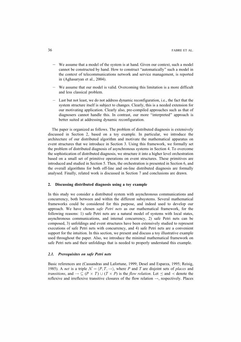
2.5. Asynchronous diagnosis with two concurrent sensors and a single supervisor

Focus on setup S2, in which alarms are recorded by two independent sensors, and then

collected at a single supervisor for explanation. Figure 6 shows the same alarm history as

in Figure 4, except that it has been recorded by two independent sensors, respectively

attached to each component. The supervisor knows the global model of the system, we

recall it in the 1st diagram of Figure 6.

The two Brepair^ actions are now distinguished since they are seen by different

sensors, this is why we use different labels: �1, �2. This distinction reduces the am-

biguity: in Figure 6 we suppress the white filled path (2) ! � ! (1) that occurred in

Figure 5. On the other hand, alarms are recorded as two concurrent sequences, one for

each sensor, call the whole an alarm pattern. Causalities between alarms from different

components are lost. This leads to further ambiguity, as shown by the additional

configuration �3 that can explain the alarm pattern in Figure 6, compare with Figure 5.

The valid explanations for the entire alarm pattern are the three configurations �1, �2 and

�3 filled in dark gray in the 3rd diagram. To limit the complexity and size of the figures,

we will omit the Blong^ configuration �3 in the sequel.

1 Strictly speaking, our projection operation creates two respective clones of �1 and �2 by exchanging, in (3),

the two lines explaining the �-alarms. But the two resulting pairs of isomorphic configurations are fused by our

Btrimming[ operation, hence we did not show these clones.

44 FABRE ET AL.

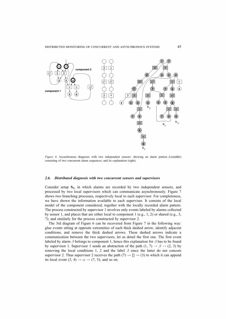
2.6. Distributed diagnosis with two concurrent sensors and supervisors

Consider setup S3, in which alarms are recorded by two independent sensors, and

processed by two local supervisors which can communicate asynchronously. Figure 7

shows two branching processes, respectively local to each supervisor. For completeness,

we have shown the information available to each supervisor. It consists of the local

model of the component considered, together with the locally recorded alarm pattern.

The process constructed by supervisor 1 involves only events labeled by alarms collected

by sensor 1, and places that are either local to component 1 (e.g., 1, 2) or shared (e.g., 3,

7); and similarly for the process constructed by supervisor 2.

The 3rd diagram of Figure 6 can be recovered from Figure 7 in the following way:

glue events sitting at opposite extremities of each thick dashed arrow, identify adjacent

conditions, and remove the thick dashed arrows. These dashed arrows indicate a

communication between the two supervisors, let us detail the first one. The first event

labeled by alarm � belongs to component 1, hence this explanation for � has to be found

by supervisor 1. Supervisor 1 sends an abstraction of the path (1, 7) ! � ! (2, 3) by

removing the local conditions 1, 2 and the label � since the latter do not concern

supervisor 2. Thus supervisor 2 receives the path (7) ! [] ! (3) to which it can append

its local event (3, 4) ! � ! (7, 5); and so on.

Figure 6. Asynchronous diagnosis with two independent sensors: showing an alarm pattern A (middle)

consisting of two concurrent alarm sequences, and its explanation (right).


Fig

ure

7.

Dis

trib

ute

dd

iag

no

sis:

con

stru

ctin

gtw

oco

her

ent

loca

lv

iew

so

fth

eb

ran

chin

gp

roce

ssU P

;Ao

fF

igu

re6

by

two

sup

erv

iso

rsco

op

erat

ing

asy

nch

ron

ou

sly

(fo

rsi

mp

lici

ty,

con

fig

ura

tio

n�

3o

fF

igu

re6

has

bee

no

mit

ted

.)

46 FABRE ET AL.

Discussion: handling asynchronous communications. The cooperation between the two

supervisors needs only asynchronous communication. Each supervisor can simply Bemit

and forget.^ Diagnosis can progress concurrently and asynchronously at each supervisor.

For example, supervisor 1 can construct the branch [1 ! � ! 2! �1! 1! � ! 2]

as soon as the corresponding local alarms are collected, without ever synchronizing with

supervisor 2. Assume some (finite but possibly unbounded) communication delay between

the two supervisors. Consider the explanations of the second occurrence of alarm � by the

1st supervisor (there are three of them). The left most two do not require any synchronization

with the supervisor 2. Thus they can be produced as soon as the local alarm sequence �, �1,

� has been observed, independently from what supervisor 2 is doing, i.e., concurrently with

supervisor 2. In contrast, the right most explanation needs to synchronize with supervisor 2,

since it waits for the abstraction (3)![]!(7) sent by supervisor 2. Thus this third

explanation may suffer from some (finite but possibly unbounded) communication delay.

However this will not impact the production of the first two explanations. This perfectly

illustrates how a concurrency approach allows to handle asynchronous communications. This

should be compared with the approaches proposed in (Debouk et al., 2000; Genc and

Lafortune, 2003) where essentially synchronous communications, from sensors to super-

visors and between the different supervisors, is required.

3. Event structures and their use in asynchronous diagnosis

In Section 2.4 we announced the need to consider event structures. This section is

devoted to their introduction for the purpose of asynchronous diagnosis.

3.1. Prime event structures

Running example, continued. Figure 8 shows in (a) the 1st diagram of Figure 5. Focus

for the moment on the topological structure of this diagram by ignoring labels, and add

an initial event: this yields the net (b). In net (b), sources of conflicts are either

mentioned explicitly, or inferred from the graph topology by searching for downward

branching conditions. This dual way of indicating confict is not elegant. Thus, we

prefer to omit conditions and represent explicitly all sources of conflicts between

eventsVconflict will be inherited by causality. Performing this yields the event

structure depicted in (c), where the down-going branches indicate causality, and sources

of conflict are explicitly indicated. In this structure, the information regarding labels has

been lost. We shall show later how to add it properly to diagram (c). ÍWe are now ready to introduce the mathematics of event structures.

Prime event structures: formal definition. Event structures havebeen introduced in (Nielsen

et al., 1981), and further extensively studied by G. Winskel (1982, 1987) and several authors

since then. Several classes of event structures have been proposed, by relaxing the conditions

required on the conflict relation and/or exchanging the causality relation for a more general

Benabling^ relation. Equipping prime event structures with parallel composition has been


recognized quite complex. An inductive definition is presented in (Degano et al., 1988).

Indirect, non inductive, definitions have been proposed by G. Winskel (1987). F. Vaandrager

(1989) has proposed a simple direct, non inductive, definition, in categorical style. This

definition suits our needs. Here we summarize the results from Vaandrager (1989), with

minimal changes in the notations.

A prime event structure2 is a triple E ¼ E;; #ð Þ, where E is a set of events, is a

partial order on E such that for all e 2 E, the set {e0 2 E j e0 e} is finite, and # is a

symmetric and irreflexive relation on E such that for all e1, e2, e3 2 E, e1#e2 and e2 e3

imply e1#e3.3 Each subset of events F � E induces a substructure E jF ¼ F;F ; #F Þð , by

restricting to F the relations and #.

As usual, we write e � e0 for e e0 and e m e0. We write dee for the set {e0 2 Eje0 e}

and we call it the configuration generated by e. For E ¼ E;; #ð Þ an event structure, a

subset X of E is called causally closed if e 2 X implies dee � X. Subset X is called

conflict-free if no pair of elements of X are in conflict, i.e., X � X 7 # = ;. A

configuration is a causally closed conflict-free subset of E. Each event structure

E ¼ E;; #ð Þ induces a concurrency relation defined by e � e0 iff neither e e0 nor e0 e nor e#e0 holds. A subset X of concurrent events is called a co-set.

Morphisms. We will use partial functions. We indicate that is a partial function from X to Y

by writing : X 7!? Y. The domain of is denoted by dom( ). Since (x) may not be defined

for x 2 X, we indicate this by writing (x) = ?, thus symbol B?^ is to be interpreted as

Bundefined.^

2 From now on, when referring to prime event structures, we shall omit the term Bprime,[ unless it is required

for the point being discussed.3 Obviously, restricting an occurrence net to its set of events yields a prime event structure. This is the usual

way of associating nets and event structures, and explains the name.

Figure 8. The informal labeled occurrence net (a), taken from Figure 4, 3rd diagram (conditions are figured by

circles and events are figured by boxes). Erasing the labels of events and adding an initial event yields the net

(b). The resulting event structure is shown in diagram (c).

48 FABRE ET AL.

For : X 7!? Y and X 0 � X ; set ðX 0Þ ¼def f ðxÞ j x 2 X 0g: ð4Þ

A morphism from E1 to E2 is a partial function : E1 7!? E2 such that:

8ðe1; e2Þ 2 E1 � E2 : e2 �2 ðe1Þ ) 9e01 2 E1; e01 �1 e1 and ðe01Þ ¼ e2 ð5Þ

8e1; e01 2 E1 : ðe1Þ#2 ðe01Þ or ðe1Þ ¼ ðe01Þ ) e1#1e01 or e1 ¼ e01 ð6Þ

Conditions (5,6) state that morphisms can erase but cannot create causalities and conflicts.

Condition (5) can be equivalently reformulated as follows:

8e1 2 E1 : e1ð Þ defined) e1ð Þd e � e1d eð Þ ð7Þ

and the following result is proved in Vaandrager (1989):

X is a configuration of E1 ) ðX Þ is a configuration of E2; ð8Þit shows that morphisms are indeed a natural notion. In (Vaandrager, 1989) it is proved that

prime event structures with morphisms of event structures form a category E with the usual

composition of partial functions as composition and the identity functions on events as identity

morphisms.

3.2. Labeled event structures and trimming

As discussed at the end of Section 2, we are mainly interested in event structures

originating from net unfoldings. The homomorphism ’ mapping unfolding UP to P yields

a natural labeling of the events of UP in terms of transitions of P. Thus, net unfoldings

induce naturally event structures in which events are labeled by transitions of P.

However, as seen from the illustrative example of Section 2, interactions between

components and supervisors occur via shared places, and diagnosis is naturally expressed

in terms of sequences of markings. Therefore transitions of the underlying Petri nets

play little role in distributed diagnosis. Hence, we shall rather label events of UP by

the post-set of their associated transition. Formally,

we label event e 2 UP by ’ðeÞ� 2 PowðPÞ; ð9Þ

where Pow denotes the power set.

Running example, continued. Diagram (c) of Figure 9 shows how labels of the form (9)

can be inserted in our case. The reader is invited to reconsider Figures 4Y7 by making

systematically the changes (a) 7!(b) 7!(c). ÍThe above discussion motivates the special kind of labeling we formally introduce now.

Labeling. For E ¼ E;; #ð Þ an event structure, a labeling is a map

� : E 7!Pow Pð Þn ;f g ð10Þ


where P is some finite alphabet; we extend (10) by convention by putting �(?) = ;.Labeled event structures are denoted by E ¼ E;; #; �;Pð Þ, and P is called the label set,

by abuse of notationVthe reader is kindly asked to remember that labels are subsets, not

elements of label set P. We shall not distinguish labeled event structures that are

identical up to a bijection that preserves labels, causalities, and conflicts; such event

structures are considered equal, denoted by the equality symbol =. The notions of

substructure and morphism need to be revisited to accommodate for labeling.

Substructure. Let E ¼ E;; #; �;Pð Þ be a labeled event structure, and let F � E and

Q � P. Pair (F, Q) induces the substructure

E jF;Q ð11Þ

having EF,Q ¼def{e 2 F j �(e)7Q m ;} as set of events, and �F,Q(e) = �(e)7Q as labeling

map. The causality and conflict relations are inherited by restriction.

Morphisms. For Ei ¼ Ei;i; #i; �i;Pið Þ; i 2 1; 2f g two labeled event structures such

that P2 � P1, a morphism is a partial function : E1 7!? E2 satisfying conditions (5,6),

plus the following monotonicity condition regarding labels:

8e1 2 E1 \ dom ð Þ : �2 e1ð Þð Þ ¼ �1 e1ð Þ \ P2: ð12Þ

By (12) and since events different from ? must have a non empty label, we know that

dom( ) � {e1 2 E1 j �1(e1) 7 P2 m ;}. A morphism satisfying

dom ð Þ ¼ e1 2 E1 j�1 e1ð Þ \ P2 6¼ ;f g ð13Þis called a strong morphism. Strong morphisms compose. Thus we can consider two

categories of labeled event structures, namely:

� The category Es

of labeled event structures equipped with strong morphisms.

Figure 9. Adding labels to event structures. Following (9), the event structure of Figure 5 has been enriched

with the labels of the postset of each event.

50 FABRE ET AL.

� The category Ew

of labeled event structures equipped with weak morphisms, i.e.,

morphisms satisfying (12) but not necessarily (13).

Most results we give below apply to both categories. To avoid mentioning

systematically Bstrong^ or Bweak,^ we will simply refer to the category of labeled

event structures E equipped with morphisms. This will refer either to Es

or to Ew

, in a

consistent manner. A few results will hold for only one of these two categories; we will

make this explicit in each case.

Trimming and Reduction. When discussing our example, we have indicated that

unnecessary replicas of parts of the diagnosis can occur. Here we discuss how to

remove these. Figure 10 shows in (a) a replica of 1st diagram of Figure 5 with its

suggestion for Btrimming.^ Diagram (b) shows the labeled event structure corresponding

to (a). Finally, diagram (c) shows the result of applying, to (b), the trimming operator

defined next. ÍLet E ¼ E;; #; �;Pð Þ be a labeled event structure. Denote by ! the successor relation,

i.e., the transitive reduction of the relation . For e 2 E, we denote by �e the preset of e

in (E, !). Then, E is called trimmed iff it satisfies the following condition:

8e; e0 2 E :�e ¼ �e0

and �ðeÞ ¼ �ðe0Þ

�) e ¼ e0: ð14Þ

Informally, E is trimmed iff any two configurations that have produced identical label

histories are identical. Any labeled event structure E ¼ E;; #; �;Pð Þ can be made

trimmed as explained next. Consider the following equivalence relation on confi-

gurations:

� ) �0 iff� and �0 are isomorphic;when seen as labeled partial orders.

�ð15Þ

Figure 10. Illustrating trimming.


The equivalence class of � modulo õ is denoted by �õ; it represents the label history of

the configuration �. Define the function trim by:

trim : E 3 e 7! ed e)

Informally, trim(e) is the label history causing event e to occur. Define:

trimðEÞ ¼ ðEu;u; #u; �u;PÞ; ð16Þ

where

Eu ¼ trimðEÞu ¼ �

f1#u f2 iff e1#e2 holds 8ðe1; e2Þ such that

fi ¼ trimðeiÞ holds, for i 2 f1; 2g�uð f Þ ¼ �ðeÞ iff f ¼ trimðeÞ:

ð17Þ

Informally, trim Eð Þ is obtained by inductively superimposing events that satisfy the

conditions listed on the left hand side of the bracket in (14); trim Eð Þ is a trimmed event

structure, and trim is a (total) morphism from E onto trim Eð Þ. The map trim satisfies the

following self-reproducing property on labels:

fd e ) ed e if f ¼ trim eð Þ; ð18Þ

meaning that configurations df e and dee possess identical label histories.

For E ¼ E;; #; �;Pð Þ a labeled event structure and Q � P, we write by abuse of

notation (cf. (11))

EjQ ¼def EjEQ;Q ð19Þ

where EQ = {e 2 E j �(e) 7 Q m ;}. Define the reduction of E over Q by:

RQðEÞ ¼def

trimðEjQÞ: ð20Þ

3.3. Event structures obtained from unfoldings

Let P ¼ P; T ;!;M0ð Þ be a Petri net, UP its unfolding, and ’ the associated net

homomorphism. Denote by

EP ¼ ðE;; #; �;PÞ ð21Þ

the trimmed event structure obtained by

1. labeling the events e of UP by �(e) ¼def ’ (e�);

2. erasing the conditions in UP and restricting relations and # accordingly;

3. adding an extra event e0 such that e0 e for each event e of UP and labeling e0 by

�(e0) = M0;

4. trimming the so obtained labeled event structure.

52 FABRE ET AL.

4. Distributed diagnosis: formal problem setting

We are now ready to formally state the problem of distributed diagnosis. We are given

the following labeled Petri nets:

P ¼ P;T ;!;M0; �ð Þ : the underlying Btrue^ system. P is subject to faults, thus

places from P are labeled by faults, taken from some finite alphabet (the non-

faulty status is just one particular Bfault^). The labeling map � associates, to each

transition of P, a label belonging to some finite alphabet A of alarm labels.

For its supervision, P produces so-called alarm patterns, i.e., sets of causally related

alarms.

Q ¼ PQ; TQ;!;MQ0 ; �Q� �

: Q represents the behavior of P, as observed via the

sensor system. Thus we require that: (i) The labeling maps of Q and P take their

values in the same alphabet A of alarm labels, and (ii) LQ - LP , i.e., the language

of Q contains the language of P. In general, however, Q 6¼ P. For example,

if a single sensor is assumed, which collects alarms in sequence by preserving

causalities, then Q is the net which produces all linear extensions of runs

of P. In contrast, if several independent sensors are used, then the causalities

between events collected by different sensors are lost. Configurations of Q are called

alarm patterns.

4.1. Global diagnosis

Consider the map: A 7! UA�P , where A ranges over the set of all finite alarm patterns.

This map filters out, during the construction of the unfolding UP , those configurations

which are not compatible with the observed alarm pattern A. We can replace the

unfolding UA�P by the corresponding event structure EA�P . Then, we can project

away, from EA�P , the events labeled by places from A (see Benveniste et al.

(2003a)VTheorem 1 for details). Thus we can state:

DEFINITION 1 Global diagnosis is represented by the following map:

A 7! RPðEA�PÞ; ð22Þwhere A ranges over the set of all finite configurations of Q.

4.2. Distributed diagnosis

Assume that Petri net P decomposes as P ¼ ki2 IPi. The different subsystems Pi interact

via some shared places, and their sets of transitions are pairwise disjoint. In particular,

the alphabet A of alarm labels decomposes as A = [i2 I Ai, where the Ai are pairwise

disjoint. Next, we assume that each subsystem Pi possesses its own local sets of sensors,

and the local sensor subsystems are independent, i.e., do not interact. Thus Q also

decomposes as Q ¼ ki2 IQi, and the Qi possess pairwise disjoint sets of places.


Consequently, in (22), A decomposes as A ¼ ki2 IAi, where the Ai, the locally recorded

alarm patterns, possess pairwise disjoint sets of places too.

As stated in the introduction, distributed diagnosis consists in computing the local

view, by each supervisor, of global diagnosis. This is formalized next.

DEFINITION 2 Distributed diagnosis is represented by the following map:

A 7! ½RPiðEA�PÞ0i2 I ; ð23Þwhere A ranges over the set of all finite prefixes of runs of Q. Our objective is therefore

to compute RPiEA�Pð Þ½ 0i2 I without performing global diagnosis, i.e., without computing

EA�P .

As advocated in the introduction, in order to scale up to large distributed systems, it is

requested that computing the local view, by each supervisor, of the global diagnosis, is

performed without computing the global diagnosis. In other words, we want to compute

RPiEA�Pð Þ without computing EA�P . The reader should notice that, in general,

RPiEA�Pð Þ 6¼ EAi �Pi

, expressing the fact that the different supervisors must cooperate

at establishing a coherent distributed diagnosis.

4.3. The need for a higher-level Borchestration^

The distributed diagnosis algorithm illustrated in Figure 7 is easy to understand, for our

running example. But this running example is very simple, for the following reasons:

firstly, it involves only two components, and, second, interaction occurs through the two

alternating places 3 and 7 and the interaction pattern 7! � ! 3! �! 7! � ! 3 . . .

involves no concurrency and no conflict.

Now, distributed diagnosis with several supervisors and more complex interaction

than in our toy example, results in a really messy algorithm. To scale up, we need to

better structure our algorithm. In Section 6 we provide a high-level orchestration of

distributed diagnosis. In this orchestration, details are hidden in the form of a set of

primitive operations on certain event structures. The orchestration will be formally

analyzed and proved correct. Before this, in Section 5 we formally introduce our set of

primitive operations.

5. Event structures and their use in distributed diagnosis

Running example, continued. Figure 11 shows three prefixes of the mid diagram of

Figure 7. Diagram (a) illustrates local diagnosis performed by supervisor 1 and 2,

independently, based on the observation of A1 ¼ �; �1f g and A2 ¼ �f g; it consists

in computing E1;1 ¼def EA1 �P1, at supervisor 1, and E2;1 ¼def EA2 �P2

at supervisor 2.

In (b) a messageM1;2 ¼ RP1 \ P2E1;1

� �is sent by supervisor 1 to supervisor 2; it consists

of the graph (7) ! [] ! (3) sitting at the extremity of the thick right going arrow;

this graph is Bcomposed^ with E2;1, this yields the result E2;2 shown in (b). Using E2;2,

supervisor 2 can now reuse its alarm pattern A2 and further extend E2;2; the result is

54 FABRE ET AL.

shown in (c), call it E2;3. Finally, (d) is the mirror of (b): a message M2;1 ¼RP1 \ P2

E2;3

� �is sent by supervisor 2 to supervisor 1; it consists of the longer graph (7)

! []! (3)! []! (7) sitting at the extremity of the double thick left going arrow; this

message is Bcomposed^ with E1;1 by supervisor 1, by gluing the common prefix (7)! []

! (3); this yields E1;2 shown in (d). ÍThroughout this discussion, we have used two operations: 1) the Bcomposition^ of a

received message M with the diagnosis currently available at the receiver, and 2) the

Bextension^ of a prefix of local diagnosis by re-unfolding the alarms, e.g., from E2;1 to

E2;2. The first operation will be formalized by considering the trimmed composition of

labeled event structures, studied in Section 5.1. The second operation, we call it the

Bextended unfolding,^ will be studied in Section 5.2. As we shall see, they are sufficient

to express and formally study distributed diagnosis in all cases.

5.1. Composition of labeled event structures

Focus again on Figure 11, diagrams (c) and (d). The update, from (c) to (d), shows

the kind of composition operator we need in order to formally specify our algorithm.

This operator performs two things. First, it glues the two isomorphic graphs (7) ! []

Figure 11. The detailed mechanism of off-line diagnosisVcompare with Figure 7.


! (3) occurring in thick in the left and right parts of diagram (c): this is a parallel

composition in which isomorphic parts are glued together by synchronizing events

with same label and isomorphic causes. This parallel composition will be formally

introduced below under the name of Bstrong parallel composition,^ denoted by �s.

Next, concentrate on diagram (d). Besides gluing together the two isomorphic graphs (7)

! []! (3), it extends it by appending the thick path (3)! []! (7) to the condition (3).

This is a different kind of parallel composition that performs a Bcontinuation^ of the

strong parallel composition by configurations that exist only in one component. Such

continuations will be formally defined below. Finally, combining these elementary

operations will yield a primitive called the Btrimmed composition^ and denoted by the

symbol k.

5.1.1. Parallel composition of event structures without labels

This is a classical notion, first introduced by Winskel (1982). We follow closely (Vaandrager,

1989) with minimal changes in the notations. Let Ei ¼ Ei;i; #ið Þ; i 2 1; 2f g, be two labeled

event structures. Set

E1 �? E2 ¼def fðe1; ?Þ j e1 2 E1g[ fð?; e2Þ j e2 2 E2g[ fðe1; e2Þ j e1 2 E1 and e2 2 E2g

where ? denotes a special event undefined. Denote by p1 and p2 the projections

given by pi (e1, e2) = ei for i 2 {1, 2}, respectively. Call a subset � of E1 �? E2 a pre-

configuration iff:

(i) For i 2 {1, 2}, pi (�) is a configuration of Ei;

(ii) �, the transitive closure of relation e 7(� � �), is a partial order, where e �(E1 �? E2) is defined by:

f 2 f 0 , �1ð f Þ 1 �1ð f 0Þ or �2ð f Þ 2 �2ð f 0Þ: ð24Þ

If � moreover has a unique maximal element w.r.t. �, then � is called a complete prime.

Then, the parallel composition of E1 and E2, denoted by E1 � E2, is the structure (E, , #)

with:

E ¼ f� j � is a complete primeg;� �0 , � � �0;�#�0 , � [ �0 is not a pre-configuration.

ð25Þ

It is proved in (Vaandrager, 1989) that the so defined E1 � E2 is also a prime event

structure. To conform with the usual notation for events, we shall denote by e the events of

E1 � E2 (instead of � as in (25)). With this updated notation, two canonical projections

are associated with the parallel composition: the first projection

P1 : E 7!? E1 is defined by 8e 2 E : P1ðeÞ ¼def�1ðmaxðeÞÞ; ð26Þ

56 FABRE ET AL.

and the second projection P2 is defined similarly. Note that this definition is consistent

since � is a complete prime.

Comments. The intuition behind (25) is that the product event structure is defined

indirectly through its configurations. If E1 and E2 execute in parallel, then events of E1

and E2 can either occur in isolation (this corresponds to pre-events of the form

(e1, ?) or (?, e2)), or an event of E1 can synchronize with an event of E2 (in which case

we have a pre-event of the form (e1, e2)). Now, at any stage of the execution of E1 � E2,

a set of pre-events has occurred; the notion of pre-configuration gives a characterization

of these sets. Condition (i) says that if we project a pre-configuration onto one of the two

components, the result must be a configuration of this component. Condition (ii) says

that the events of the component may occur only once and that both components must

agree on the causal relations between events in the parallel composition. Once the finite

configurations of the parallel composition have been defined, then a standard procedure

can be used to turn this into a prime event structure, namely by identifying events

of the composition with configurations having a unique maximal element. ÍThe following results are borrowed from (Vaandrager, 1989). They express that the

parallel composition of event structures is the proper notion of composition:

1. The two projections Pi, i 2 {1, 2} associated with the parallel composition of event

structures are morphisms.

2. The parallel composition E1; E2ð Þ 7! E1 � E2 with projections P1 and P2 is a

product in the category E of event structures. This product is associative and

commutative.

Statement 2 means that the parallel composition satisfies the following universal

property:

In (27), symbols i, Pi, for i 2 {1, 2}, and , denote morphisms, P1 and P2 are the

two projections associated with the composition E1 � E2, and the second diagram

commutes.

5.1.2. Parallel composition of event structures with labels

As explained in Section 3.2, formulas (12,13), two categories Es

and Ew

can be

considered, depending on the classes of morphisms. Each category has its associated

product that we define next.

Define the strong and the weak parallel composition of two labeled event structures

Ei ¼ Ei;i; #i; �i;Pið Þ; i 2 1; 2f g, denoted by E1 �s E2 and E1 �w E2, respectively. Both


are variations of the case without labels. Two events ei 2 Ei, i 2 {1, 2} are called

strongly, resp. weakly compatible, respectively written

resp.e1 ffls e2

e1 fflw e2

oiff:

�1ðe1Þ � P1nP2 and e2 ¼ ?resp. �1ðe1Þ � P1 and e2 ¼ ?

�or

�2ðe2Þ � P2nP1 and e1 ¼ ?resp. �2ðe2Þ � P2 and e1 ¼ ?

�or

�1ðe1Þ \ P1 \ P2 ¼ �2ðe2Þ \ P1 \P2 6¼ ;:

8>>>>>><>>>>>>:

ð28Þ

The first two cases correspond to an event that involves a single component, whereas the

third case corresponds to two non silent events synchronizing (their labels agree on the

shared places). Note the difference in the rules for (s and (w : for (s, a component can

progress alone by means of a private event only, whereas, for (w, the event does not

need to be private. Define

E1 �s E2¼deffðe1; e2Þ 2 E1 �? E2 j e1 ffls e2g;

E1 �w E2¼deffðe1; e2Þ 2 E1 �? E2 j e1 fflw e2g;

ð29Þ

with the convention �(?) = ;. Then the two parallel compositions E1 �s E2 and E1 �w E2

are defined via (25), but with E1 �s E2 and E1 �w E2 replacing E1 �? E2, respectively,

and, for both cases:

�ðeÞ ¼ �1ðP1ðeÞÞ [ �2ðP2ðeÞÞ; ð30Þ

where the projections Pi are defined in (26). The parallel composition is illustrated on

Figure 12. By construction,

E1 �s E2 v E1 �w E2; and PiðE1 �w E2Þ ¼ Ei; for i 2 f1; 2g: ð31Þ

Universal property (27) adapts for �s with strong morphisms, and for �w with weak

morphisms.

5.1.3. Continuations

Consider an event structure E ¼ E;; #; �;Pð Þ, a prefix F v E having F as its set of

events, and Q � P. The continuation of F by E through Q, written

F�Q E; ð32Þ

is the prefix of E consisting of the following set of events: 1) the events of F , 2) the

events e of E such that the restriction deejF,Q is a maximal configuration of F Qj (see

(11)). By definition F v F�Q E� �

v E.

The continuation is illustrated in Figure 12. For this discussion, call F the bottom left

diagram, E the bottom right one, and take Q = {3, 7}. Then, F Qj is depicted in thick in

the two bottom diagrams (except that we did not adjust the labels). The configuration of

E in light gray is a continuation of the configuration {7} of F Qj ; since configuration {7}

58 FABRE ET AL.

is not maximal in F Qj , the configuration of E in light gray is discarded in constructing

F �Q E, shown on the top right diagram.

5.1.4. Trimmed composition

Our final primitive operation for use in orchestrations will be the trimmed composition of

an indexed family Ei; i 2 I , of labeled event structures, defined by:

ki2 I Ei ¼deftrim

�Ps

i2 I Ei

��Q Pw

i2 I Ei

�Þ; ð33Þ

Figure 12. Parallel composition of labeled event structures. The first two diagrams show two components that

are prefixes of the ones of Figure 7. The two diagrams sitting on the bottom show the �s- and �w-compositions.

The resulting k-composition is shown on the top right diagram.


where Ps and Pw refer to the �s and �w compositions, respectively, and

Q ¼ interact Pið Þi2 I ¼def [ i; jð Þ 2 I � I :i 6¼ j Pi \ Pj

� �:

ð34Þ

Note that k, regarded as a binary operator, is not associative. This is why we define the

trimmed composition as an n-ary operator directly.

Running example, continued. Construction E1 k E2 is illustrated in Figure 12. Recall

that 3 and 7 are the shared places. The third diagram of this figure shows the �s-

composition; the branch [3] ! [7, 5] that is offered by component 2 finds no counterpart

in component 1, hence it does not appear in the �s-composition. For the k trimmed

composition, it is allowed to continue maximal configurations of the �s-composition

with configurations that exist in the more permissive �w-product. Now, the branch [3]![7, 5] ! [4] that is offered by component 2 contributes to the �w-product. It

continues the configuration [7]! [3] that is maximal in the restriction E1 � s E2ð Þ jP1 \ P2.

Therefore it gives raise, in the k-composition, to the extension [2, 3] ! [7, 5] ! [4] of

the �s-product.

Note that, projecting away, from this k-composition, the labels 5, 6, 4 that are private

to the 2nd component yields exactly the left diagram of Figure 11-(d).

Star closure. Consider again Figure 11. In (d), diagram E1;1 is receiving � ¼def(7)! []

! (3) as an Becho^ of its own message sent in (b). This means that, in (d), a composition

�k� occurs. And this scheme is repeated throughtout the different steps of the informal

algorithms shown in Figure 7. Therefore, we need to pay attention to how E k E relates

to E, for E an arbitrary event structure.

Despite the notation that seems to refer to the conjunction in logic, the operator k is

not idempotent: we do have E v E k E, but equality does not hold in general. The reason

is the following: assume that E contains two different configurations �1 and �2 such that

there exists a bijective map �, from the set of events of �1 to the set of events of �2,

which is label preserving and such that �; �ð Þ j�1

� � �[ j�2

generates a partial

orderVsaid differently, the two orders on each configuration do not contradict each

other. Then, � ¼def{(e1, �(e1)) j e1 2 �1} is a preconfiguration of E �s E that has no

counterpart in E. Thus, as soon as such pathological pairs of non-contradictory

configurations exist in E, we have E 6¼ E �s E and thus also E 6¼ E k E. The above

discussion also reveals that the gap between E and E ; j E is indeed small, since it consists

only in Breshuffling^ pairs of non-contradictory configurations to form new ones. This

leads to considering the star closure of event structures we introduce next.

Write En ¼defE j . . .j jj E (n times). The sequence Enð Þn51 is increasing for the prefix

order, and converges to a unique event structure,

we denote it by E* and call it the star closure of E: ð35Þ

The star closure E* is the minimal (for prefix order) solution of the fixpoint equation

X ¼ E Xk . It satisfies E*� �n ¼ E* for each n Q 1, and, for each event structure F , we

have F v E kF iff F v E*.

60 FABRE ET AL.

Important properties of event structures and their composition are collected in

Appendices A.1 and A.2.

5.2. Extended unfoldings

In Section 3.3 we have introduced the event structure EP associated to the unfolding

of a Petri net P. In this section we generalize EP to situations in which the considered

Petri net P is unfolded, starting from a given initial labeled event structure I . This

construction was used in step (c) of Figure 11.

Let P ¼ P; T ;! ;M0ð Þ be a Petri net. For M � P, call PM the Petri net P in which M

has been substituted for the initial marking M0 of P (note that we do not require that M

should be reachable from M0). Write for short EM ¼def EPM . Each event e 2 EM represents

some set Te of transitions of P (Te may not be a singleton, due to the trimming performed

when mapping UP to EP). For each t 2 Te, t� = �(e).

Let I be a labeled event structure having Q - P as label set. Denote by � the labeling

map of I . For I a co-set of I such that �(i) 7 P m ; holds for each event i 2 I, set M ¼def

[i2 I (� (i) 7 P). A total map � : M 7! I such that p 2 � (�(p)) is called a representation

of M by I. Denote by Mz� I the set of all such representations. We shall Bappend^ EM to

I via � as follows.

Denote by e0,M the minimal event of EM . Denote by EI ;�;M the event structure obtained

by taking the disjoint union of I and EMn e0;M

� , and adding the following causalities:

For each event i of I and each event e of EM such that e 2 e�0, M, set

e 2 i� in EI ;�;M if 9t 2 Te; 9p 2�t; such that i ¼ � pð Þ:

Let I be the set of all co-sets I of I such that � (i) 7 P m ; holds for each event i 2 I. The

unfolding of P from I , written EIP , is defined by:

EIP ¼def

trim I [[

I2 I;�2M ,! �I

EI ;�;M

" # !; where M ¼def

[i2 I

� ið Þ ð36Þ

Note that the trimming is essential here, since the expression in parentheses in formula

(36) exhibits lots of redundancies. The extended unfolding satisfies the following

properties, where S denotes an arbitrary label set:

I v I0 and 9P00 : P0 ¼ P jj P00 ) I v EIP v EI0

P0 ð37Þ

RS EIP� �

¼ RS ERS Ið ÞP

� �ð38Þ

Running example, continued. The right hand side of diagram (c) of Figure 11

shows E2;3 ¼ EIP for I E2;2 and P A2;1 � P2 where symbol @ denotes

substitution. ÍImportant properties of extended unfoldings are found in Appendix A.3.


5.3. Detailed Implementation of the Primitives

In this section, we provide effective implementations of our primitives by means of

pattern matching rules.

Parallel compositions �s and �w. Recall that the parallel compositions �s and

�w of labeled event structures are defined via formulas (25,29,30). Write X ï e if X -�e, and say that X enables e. The parallel composition E1 �sE2 is constructed by

inductively applying the following rule, in which X denotes a (possibly empty) co-set

of E1 �sE2:

P1ðX Þ ‘ e1 and P2ðX Þ ‘ e2

e1 ffls e2

X is minimal having the above properties

9=; ) X ¼ �ðe1; e2Þ; ð39Þ

meaning that event (e1, e2) is a new extension of E1 �s E2 beyond co-set X. The rule for

�w is identical, except that (s is replaced by (w.

Trimming. The event structure trim Eð Þ is constructed by inductively applying the

following rule, in which Xi, i 2 {1, 2} denote (possibly empty) co-sets of trim(E ):

trimðX1Þ ¼ trimðX2Þ8i 2 f1; 2g : Xi ¼ �ei

�ðe1Þ ¼ �ðe2Þ

9=; ) trimðe1Þ ¼ trimðe2Þ ð40Þ

The following canonical form can be considered for a labeled trimmed event structure.

Its events have the special inductive form (X, ‘ ), where X is a co-set of E and ‘ 2 Pow (P).

The causality relation is simply encoded by the preset function �(X, ‘ ) = X, and the

labeling map is ’ (X, ‘ ) = ‘. Events with empty preset have the form (nil, ‘ ). The conflict

relation is specified separately.

Trimmed Composition k. The trimmed composition E1 jj E2 is constructed by

inductively applying the following two rules, in which X denotes a (possibly empty) co-set

of E1 jj E2:


e1 ffls e2


9=; ) X ¼ � ðe1; e2Þ; ð41Þ


e1 fflw e2


9=; ) X ¼ � ðe1; e2Þ; ð42Þ

62 FABRE ET AL.

As the reader can easily check, rules (41) and (42) overlap. To ensure that only maximal

configurations obtained by using �s are further extended by means of �w, we give higher

priority to rule (41), thus making the choice between the two rules deterministic.

Extended Unfolding. The extended unfolding EIP is constructed by inductively applying

the following rule, where I is the initial condition and X denotes a co-set of EIP :

�ðX Þ - m

m ¼ �t in Petri net Pt� ¼ ‘ in Petri net P


9>>=>>; ) X ¼ � ðX ; ‘Þ; ð43Þ

6. Orchestration of distributed diagnosis

We are now ready to state our orchestration. Throughout this section, we assume the

setup of Section 4.2. Petri net P ¼ P; T ;!;M0ð Þ decomposes as P ¼ jj i2 IPi, where

Pi ¼ Pi; Ti;!;Mi;0

� �.

Completeness. Let P ¼ P; T ;!;M0ð Þ be a safe Petri net, and let Q � P. P is called Q-

complete if, for every place p 2 Q such that �p [ p� m ;, there exists a place p 2 Q such

that (i) p� ¼ �p n p�, (ii) �p ¼ p� n �p, and (iii) M0ðpÞ þM0ðpÞ ¼ 1, where M0 denotes

the initial marking. We say that P is complete if it is P-complete. If P is not Q-complete,

we can make it Q-complete by adding the missing places and arcs. The so obtained

completion P produces an event structure EP such that ðEPÞ jP ¼ EP , i.e., erasing the

place p from the event structure generated by P yields the event structure generated by

P, see Section 3.3. Informally said, completion does not change the behaviour of the

Petri net. Our example P ¼ P1 jj P2 of Figure 2 satisfies this property with Q = {3, 7},

since places 3 and 7 are complementary.

Distributed conflict. We say that P1 jj P2 has no distributed conflict if:

8p 2 P1 \ P2 9i 2 1; 2f g : p� � Ti: ð44Þ

Note that our example of Figure 2 satisfies (44). This is a reasonable assumption in our

context, since shared places aim at representing the propagation of faults between

components; having distributed conflict would have little meaning in this case. The

following assumption will be used in the sequel:

ASSUMPTION 1 Decomposition P ¼ jj i 2 IPi involves no distributed conflict and P is

complete.

For jj i 2 IPi a parallel composition of safe Petri nets satisfying Assumption 1, then

8p 2 Pi \ Pj if i 6¼ j then p� Ti )�p Tj: ð45Þ


6.1. Off-line orchestration of distributed diagnosis

In this section we study off-line diagnosis, meaning that some finite alarm pattern A is

given for diagnosis. The structure of the interaction between the different components Pi,

for i 2 I, will play an important role for our distributed diagnosis algorithm. This is

captured by the notion of interaction graph we introduce next.

Equip I � I with the following undirected graph structure: draw a branch (i, j) iff Pi 7

Pj m ;, i.e., the ith and jth subsystems interact directly via shared places. Denote by GI the

resulting interaction graph. For i 2 I, denote by N(i) the neighborhood of i, composed of

the set of j’s such that j 6¼ i and ði; jÞ 2 GI . Note that N(i) does not contain i.

Algorithm 1 shown in Figure 13 performs distributed diagnosis (see (23)). It consists

of a chaotic, unsupervised, cooperation between the different supervisors acting as peers.

It is expressed in terms of the primitives EIP (to continue local diagnosis), RQ (to model

the relevant information for the interfaces of a subsystem), and k (to compose messages

from other supervisors with current local diagnosis). This algorithm is analysed in the

following two theorems.

ALGORITHM 1 Each site i maintains and updates, for each neighbor j, a message Mi; j

toward j. Thus there are two messages per edge (i, j) of GI , one in each direction. The

algorithm consists of chaotic iterations as follows:

Figure 13. Algorithm 1. Symbol := denotes assignment.

64 FABRE ET AL.

THEOREM 1 Algorithm 1 is monotonic (i.e., the Ei’s andMi; j’s are increasing w.r.t. the

prefix order), confluent, and converges in finitely many iterations.

Proof: The monotony of Algorithm 1 results from the following properties: 1)

I v EIP , by (37), and 2) monotony of k, by (60) from Corollary 1 of Appendix A.2.

For the proof of the confluence, it will be convenient to encode schedulings of

the three possible choices (2b), (2c), and (2a) by words. To this end, consider the

alphabet

@ ¼ ai j i 2 If g [ bi; j; bj;i j i; jð Þ 2 G��

[ ci j i 2 If g; ð47Þ

where a, b, c refer to the three different steps of Algorithm 1, and the index

refers to the edge (i, j) or the node i that is selected in the corresponding step. @*

denotes the Kleene closure of @. Denote by E �ð Þ the collection ðEiÞi 2 I obtained

after having applied scheduling � 2 @*. Clearly, Eð�Þ v Eð� < �0Þ and E �0ð Þv E � < �0ð Þ, where the prefix relation is taken componentwise and � I �0 is the

concatenation of � and �0. From this, the confluence follows immediately. This proves

the theorem. ÍSo far we did not use the structure of the interaction between the different components.

The next theorem makes deeper use of this structure. For this result we use the notion of

star closure of the k composition, introduced in (35).

THEOREM 2 Assume Assumption 1 is enforced and the interaction graph GI is a tree.

Then, if ðEiÞi 2 I denotes the limit of Algorithm 1, we have

8i 2 I : RPiEA�Pð Þ v Ei v RPi

E=A�P� �

: ð48Þ

Proof: See Appendix B.4. ÍTheorem 2 expresses that Algorithm 1 computes all solutions (23) of distributed

diagnosis, plus some extra configurations that are obtained by re-shuffling non

contradictory solutions as explained in (35).

Note that hierarchical architectures satisfy the assumptions of Theorem 2, but this

result covers more architectures than just hierarchical ones. When GI is not a tree, further

Bechoes^ result from messages confluing through different routes. The resulting case is

studied, in a more abstract context, in (Fabre, 2003).

6.2. On-line orchestration of distributed diagnosis

Now, instead of our local alarm patterns ðAiÞi2I being given once and for all, we are

given, for each i 2 I, a local set Ai of alarm patterns. We assume that Ai is totally


ordered by the prefix relation. In the sequel, the statement Bupdate Ai^ means that we

take the next alarm pattern of Ai, for the prefix order.

Running example, continued. Referring to Figure 6 or Figure 7, the total ordering of

alarm patterns is depicted by regarding the partially ordered alarm pattern as a labeled

graph directed downwards. Figure 14 shows three prefixes of the mid diagram of

Figure 7. Diagram (a) illustrates local diagnosis performed by supervisor 1 and 2,

independently, based on the observation of A1;1¼ f�g and A2;1 ¼ �f g; it consists in

computing EA1;1 �P1, at supervisor 1, and EA2;1 �P2

at supervisor 2. In (b) a messageM1;2

is sent by supervisor 1 to supervisor 2. Using this message, supervisor 2 can now reuse its

A2;1 and extend EA2;1 �P2; the result is shown in (c), it is equal to RP2

EA1 �Pð Þ, namely

the local view, by supervisor 2, of the global diagnosis having observed

A1¼def A1;1 k A2;1. ÍTo adjust for this situation, Algorithm 1 is modified to Algorithm 2 of Figure 15.

Algorithm 2 is said to be fairly executed if it is applied in such a way that each of the

three cases (a), (b), or (d), with every node i, and case (c) with every edge (i, j), are

selected infinitely many times.

Figure 14. Illustrating on-line diagnosis. The four diagrams are prefixes of the mid diagram of Figure 7;

referring to Algorithm 2, (a) illustrates case 2(a) illustrates the transmission of a message, and (c) illustrates

case 2(b), and (d) illustrates once more case 2(a).

66 FABRE ET AL.

THEOREM 3 Assume Assumption 1 is enforced, GI is a tree, and Algorithm 2 is fairly

executed. Then, for any given A ¼ jj i2 IAi, where Ai 2 Ai, after sufficiently many

iterations, one has 8i 2 I : Ei w RPiEA�Pð Þ.

Theorem 3 expresses that, modulo a fairness assumption and with some delay,

Algorithm 2 provides, as a prefix of the current event structure it computes, the diagnosis

RPiEA�Pð Þ of any given alarm pattern A.

Proof: Monotony of Algorithm 2 is proved in the same way as for Algorithm 1. To

study the confluence of Algorithm 2, we reuse the method and notations of the proof of

Theorem 1. In particular, we adapt in an obvious way, to Algorithm 2, the coding (47)

used for the schedulings of Algorithm 1.

Denote by E �ð Þ the collection Eið Þi2 I obtained after having applied scheduling � 2 @*.

Clearly, E �ð Þ v E � < �0ð Þ and Eð�Þ v E � < �0Þð , where the prefix relation is taken

componentwise and � I �0 is the concatenation of � and �0. This is a kind of confluence

property for our on-line algorithm.

Using this property, we can chose any particular scheduling. Systematically apply (2a)

until Ai has been read for each i 2 I, then switch to the other cases, the resulting

Figure 15. Algorithm 2.


scheduling just yields the batch Algorithm 1. Hence, for this scheduling, Theorem 3 is

just Theorem 2. Í

7. Related work

This paper provides contributions to two different topics: distributed diagnosis, and event

structures. For each topic we discuss related work.

7.1. Distributed diagnosis

Fault diagnosis in discrete event systems has attracted significant attention, see (Debouk

et al., 2000) and (Sampath et al., 1995) for the diagnoser approach. Distributed diagnosis

has been less investigated. A first class of studies consider synchronous communications.

In (Genc and Lafortune, 2003) distributed diagnosis for Petri nets with synchronous

communication is studied. Trading local computations for communications is analysed in

(Boel and van Schuppen, 2002). In (Su et al., 2002; Su, 2004), distributed diagnosis with

synchronous product is studied in the linguistic framework of Wonham and Ramadge.

Global and local consistency are introduced; global consistency means that local

diagnoses are projected versions of global diagnosis, whereas local consistency only

requires that local diagnoses agree on their mutual interfacesVthe latter is an interesting

concept, not considered in our paper.

Pencole et al. (2002) study a more hybrid architecture consisting of synchronously

communicating automata and a supervisor that communicates with the subsystems

asynchronously. The solutions computed involve additional non-determinism due to the

asynchrony of the communications with the supervisor.

The book (Lamperti and Zanella, 2003) proposes a different approach, more in the

form of a simulation guided by the observed alarms, for a model of communicating

automata, see also (Baroni et al., 1999). The considered systems are networks of

automata interconnected by finitely buffered communications. The problem addressed is

that of constructing all correlation scenarios that causally relate faults and observed

alarms, for given finite alarm sequences. Monolithic and distributed diagnosis are both

considered. This approach shares similarities with ours. In particular, the active spaces

resemble our unfoldings, without, however, the handling of concurrency. A very

interesting idea is proposed to handle unobservable transitions (which we did not

consider here): cast in our framework, it consists in not unfolding unobservable loops in

the executions of the systems. This allows to keep active spaces finite, even in the

presence of loops of unobservable transitions. This is a nice idea that could be reused in

our framework. Also, the modular construction of active spaces is studied. The

associated architecture is not peer-to-peer but fully hierarchical: there is a single

coordinator that communicates with the local diagnosers and performs the fusion of

local diagnoses. Even though this is a simpler situation than ours, distributed

algorithms are (and have to be) complicated. Still, they are described at a fine grain

level, and not by using higher level primitives as we did.

68 FABRE ET AL.

Our results were announced in (Aghasaryan et al., 2002). Asynchronous diagnosis using

unfoldings was presented in (Benveniste et al., 2003a). Modeling and diagnosis of distributed

systems was first introduced in (Fabre et al., 2002; Fabre et al., 2002a, 2002b). Diagnosability

for systems with concurrency is discussed in (Haar et al., 2003). A systematic study of chaotic

algorithms such as used in this paper is performed in (Fabre, 2003), including the case of GI

not being a tree. A first version of this paper was given in (Fabre et al., 2003).

7.2. Event structures

Event structures and unfoldings were first introduced by Glynn Winskel in his thesis, see

also (Nielsen et al., 1981) and the seminal paper (Winskel, 1982). Unfoldings were

subsequently studied in (McMillan, 1992; Engelfriet, 1991; Esparza and Romer, 1999),

with applications to model checking.

Equipping prime event structures with parallel composition has been recognized

difficult. An inductive definition is presented in (Degano et al., 1988). Indirect, non

inductive, definitions have been proposed by G. Winskel, (1987). F. Vaandrager, (1989)

has proposed a simple direct, non inductive, definition, in categorical style. This is the

construction we used here.

Categorical properties of event structures and unfoldings were given in (Winskel,

1985). In particular, the mapping P 7! UP is shown to satisfy UP1 �P2¼ UP1

� s UP2,

expressing that P 7! UP is a functor. Unfortunately, there exists no simple way to

compute UP1 kP2, as we have seen. That unfoldings are functors w.r.t. the synchronous

product of nets and unfoldings suggests another approach to distributed diagnosis, in

which subystems interact via shared transitions, not places. This gives rise to a different

distributed algorithm, in which local diagnosers Bover-estimate^ solutions, and peer-to-

peer cooperations between supervisors aim at keeping only local solutions that

Bsynchronize well,^ i.e., agree on their interfaces. In contrast, in our distributed

algorithm, local diagnosers Bunder-estimate^ solutions (see (66)), and peer-to-peer

cooperations between supervisors aim at extending local solutions to reach global

consistency. Such an approach by synchronous product is precisely studied in (Fabre,

2002b). Despite the use of synchronous products, we insist that the approach of (Fabre,

2002b) assumes asynchronous communication, since partial order models are considered.

Regarding event structures per se, this paper has introduced the following new special

constructs: the �w-composition (the �s-composition is classical and simply denoted �),

the continuation, the k-composition, the generalized unfolding, and the reduction. These

special operations were needed to overcome the fact that no simple Bcategorical^ way of

computing UP1 kP2exist.

8. Conclusion

For the context of fault management in SDH/SONET telecommunications networks, a

prototype software implementing the method was developed in our laboratory, using Java

threads to emulate concurrency. This software was subsequently deployed at Alcatel on a


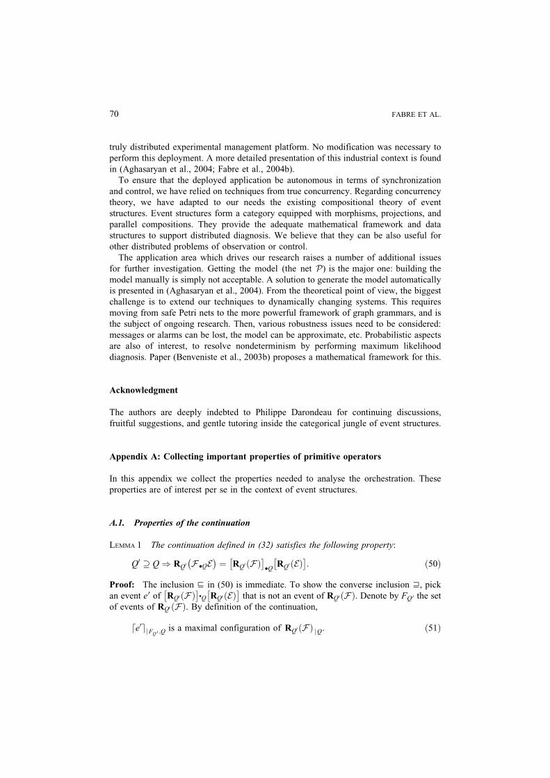
truly distributed experimental management platform. No modification was necessary to

perform this deployment. A more detailed presentation of this industrial context is found

in (Aghasaryan et al., 2004; Fabre et al., 2004b).

To ensure that the deployed application be autonomous in terms of synchronization

and control, we have relied on techniques from true concurrency. Regarding concurrency

theory, we have adapted to our needs the existing compositional theory of event

structures. Event structures form a category equipped with morphisms, projections, and

parallel compositions. They provide the adequate mathematical framework and data

structures to support distributed diagnosis. We believe that they can be also useful for

other distributed problems of observation or control.

The application area which drives our research raises a number of additional issues

for further investigation. Getting the model (the net P) is the major one: building the

model manually is simply not acceptable. A solution to generate the model automatically

is presented in (Aghasaryan et al., 2004). From the theoretical point of view, the biggest

challenge is to extend our techniques to dynamically changing systems. This requires

moving from safe Petri nets to the more powerful framework of graph grammars, and is

the subject of ongoing research. Then, various robustness issues need to be considered:

messages or alarms can be lost, the model can be approximate, etc. Probabilistic aspects

are also of interest, to resolve nondeterminism by performing maximum likelihood

diagnosis. Paper (Benveniste et al., 2003b) proposes a mathematical framework for this.

Acknowledgment

The authors are deeply indebted to Philippe Darondeau for continuing discussions,

fruitful suggestions, and gentle tutoring inside the categorical jungle of event structures.

Appendix A: Collecting important properties of primitive operators

In this appendix we collect the properties needed to analyse the orchestration. These

properties are of interest per se in the context of event structures.

A.1. Properties of the continuation

LEMMA 1 The continuation defined in (32) satisfies the following property:

Q0 - Q) RQ0 F �QE� �

¼ RQ0 Fð Þ �

�Q RQ0 Eð Þ �

: ð50Þ

Proof: The inclusion Í in (50) is immediate. To show the converse inclusion Ï, pick

an event e0 of RQ0 Fð Þ �

�Q RQ0 Eð Þ �

that is not an event of RQ0 Fð Þ. Denote by FQ 0 the set

of events of RQ0 Fð Þ. By definition of the continuation,

e0d ejFQ 0 ;Qis a maximal configuration of RQ0 Fð Þ jQ: ð51Þ

70 FABRE ET AL.

On the other hand, there exists an event e of E such that e0 = RQ 0 (e). Using (51) and the

assumption that Q0 - Q, we deduce that deejF,Q is a maximal configuration of F jQ,

which proves (50).

A.2. Properties of labeled event structures and their parallel composition

PROPOSITION 1 For the following statements, E ¼ E;; #; � , PÞð denotes a labeled

event structure, and Ei ¼ Ei; i; #i; �i, Pið Þ; i 2 1; 2f g denote two labeled event

structures. The following formulas hold:

8Q � P : RQ trim Eð Þð Þ ¼ RQ Eð Þ ð52Þ

trim½trimðE1Þ �s trimðE2Þ0 ¼ trimðE1 �s E2Þtrim½trimðE1Þ �w trimðE2Þ0 ¼ trimðE1 �w E2Þ

�ð53Þ

8Q - P1 \ P2 :RQðE1 �s E2Þ ¼ trim½RQðE1Þ �s RQðE2Þ0RQðE1 �w E2Þ ¼ trim½RQðE1Þ �w RQðE2Þ0

�ð54Þ

Proof: See Appendix B.1. ÍCOROLLARY 1 In the following statements, symbol 1 ¼def ; denotes the empty event

structure. E; E0; E00; Ei denote arbitrary trimmed event structures with respective label sets

P, P0, P00, Pi. Label set Q is arbitrary unless otherwise specified. The following

properties hold:

E k 1 ¼ E ð55Þ

RP Eð Þ ¼ E ð56Þ

RP1RP2Eð Þð Þ ¼ RP1 \ P2

Eð Þ ð57Þ

Q - interact Pið Þi2 I ) RQ ki2 I Eið Þ ¼ki2 I RQ Eið Þ ð58Þ

1 v E ð59Þ

P0 ¼ P00 and E0 v E00 ) E0 k E v E00 k E ð60Þ

E v E0 ) 8Q : RQ Eð Þ v RQ E0ð Þ ð61Þ

Proof: To prove (55), note that E �s 1 ¼ E �w 1 ¼ E. Property (56) is immediate.

For (57), note that RP1 \ P2Eð Þ ¼def

trim EP1 \ P2ð Þ ¼ trim EP2

ÞP1ð Þ ¼def

RP1EP2ð Þ ¼ RP1

�RP2Eð Þð Þ; by Proposition 1, formula (52). For (58), note that RQ jj i 2 IEið Þ¼def

RQ Psi2 IEi

��Q0 Pw

i2 IEi

�� , where Q0 = interact (Pi)i2 I. Using (50) and the assumption

that Q - Q0, we get RQ Psi2 IEi

��Q0 Pw

i2 IEi

�� ¼ RQ Ps

i2 IEi

�� Q0 RQ Pw

i2 IEi

�� Now,

by formula (54) of Proposition 1, RQ Psi2 IEi

� �¼ trim Ps

i2 I RQ Eið Þ �

, and similarly with

Pw instead of Ps. This proves (58). Finally, monotonicity properties (59)Y(61) are

immediate. Í


LEMMA 2 The following properties hold:

8j 2 I :Pj ki2 I Eið Þ ¼ Ej and RPjki2 I Eið Þ w Ej ð62Þ

Proof: Let �j be a maximal configuration of Ej: Let Cs�j

be the set of maximal

configurations of Psi2 IEi such that Pj (�) Í �j. The following two exclusive cases

can occur.

1. There exists a maximal configuration � of Psi2 IEi that satisfies Pj(�) = �j and is also

a maximal configuration of Pwi2 IEi. Then, � is also a configuration of j i2 IEij and

Pj (�) = RPj (�) = �j holds.

2. For each � 2 C�js , Pj(�) m �j. Then �j

+ = �jj Pj (�) is non empty, and co-set min(�j+)

satisfies: Oe 2 min (�j+)¼def �j�(e) 7 Q m ;. Thus, configuration � cannot be extended

at all in the �s-product. Hence, �jQ is maximal in Psi2 IEi j Q . Thus, while performing

the k-composition, �jQ can be further extended by any maximal configuration � of

Pwi2 I Ei having � as its prefix. It remains to chose � such that Pj �ð Þ ¼ �j, and �

also satisfies RPj �ð Þ ¼ �j. This finishes the proof. Í

A.3. Properties of event structures related to unfoldings

In this paragraph we collect important properties involving the parallel composition of

event structures obtained from unfoldings.

PROPOSITION 2 Let P ¼ P1 jj P2. We have

EP v trim RP1EPð Þ � s RP2

EPð Þð Þ: ð63Þ

Proof: See Appendix B.2. ÍCOROLLARY 2 Let P ¼ k i2 IPi be a Petri net, and let Pi be the set of places of Pi. The

following property holds:

EP v ki2 I RPiEPð Þ ð64Þ

Proof: To show (64), note that Proposition 2 generalizes to more than two components,

whence EP v trim ðPsi2 I RPi

EPÞð Þ. Then, Proposition 3 used with substitution I EP ,

together with the fact that trim Psi2 I Ei

� �v jj i2 IEi, proves (64). Í

PROPOSITION 3 Assume that decomposition P ¼ k i2 IPi: satisfies assumption 1. Let Ibe a prefix of EP , and assume that I i ¼def

RPiIð Þ satisfies jj i2 II i v EP : For i 2 I

consider Ei ¼ EI i

Pi, the unfolding of Pi from I i: Then, we have:

ki2 I Ei v EP : ð65Þ

72 FABRE ET AL.

Fig

ure

16

.Il

lust

rati

ng

pro

po

siti

on

3.


Note that, for I ¼ ;, (65) boils down to

ki2 I EPiv EP : ð66Þ

Proof: See Appendix B.3. ÍRunning example, continued. Proposition 3 is illustrated in Figure 16. The first two

diagrams are taken from Figure 6; they show the two components together with the alarm

pattern recorded with two independent sensors. The 3rd diagram is a copy of the last

diagram of Figure 6 in which we discarded the long configuration �3, for readibility

purposes. The prefix filled in grey in this diagram shows the part of the diagnosis that

can be inferred by each supervisor locally, i.e., by observing its own alarms, knowing its

local model only, and without cooperating with the other supervisor. In contrast, the

white suffix requires the two supervisors to cooperate. The last diagram shows an event

structure translation of the third one, by showing RP EA�Pð Þ, and its prefix

RP1EA1 �P1ð Þ k RP2

EA2 �P2ð Þ (in grey).

Appendix B: Proofs

B.1. Proof of proposition 1:

Proof of formula (52)' By expanding the definition of the reduction, this formula is

rewritten

trim F jQ� �

¼ trim E jQ� �

; where F ¼deftrim Eð Þ ð67Þ

For this proof we need to make precise the context in which we consider trimming and

configurations: trimE ; ed eE ; and �)E , shall respectively denote the trimming function, the

configuration generated by event e, and the equivalence class of configuration � modulo

õ, in the context of E. The reader is referred to (19) for the definition of E jQ.

Set EQ = {e 2 E j� (e) 7 Q m ;}. Then E jQ possesses EQ as event set, �Q = � 7 Q as

labeling map, and inherits the causality and conflict relations from E, by restriction. For

e 2 EQ, write e ¼deftrimE jQ eð Þ. Write EQ ¼def

trim E jQ� �

. Using the self-reproducing

property (18), we get

ed eEQ) ed eEQ

: ð68Þ

On the other hand, for e 2 E, we have f ¼deftrimE eð Þ ¼ ed eE

� �)E , f has label �(e), and

F has its causality and conflict relations defined by (17). Thus F jQ has FQ ¼def

trimE eð Þ j e 2 EQ

� as set of events, and inherits the causality and conflict relations

from F , by restriction. Then, by (17), the label of trimE eð Þ in the context of F jQis equal to �(e) 7 Q = �Q(e). For f 2 FQ, set g ¼def

trimF jQ fð Þ and G ¼deftrim F jQ

� �.

Using twice the self-reproducing property (18)Vonce for each trimming operationVwe get

gd eG ) fd eF jQ ; dfeF ) ed eE ð69Þ

74 FABRE ET AL.

Restrict to Q the 2nd equivalence in (69), this yields fd eFQ) ed eEQ

. Combining the latter

formula with (68) and (69) yields dgeG õ deeEQ, which proves (67).

Proof of Formula (53)' We only prove the �s case, the �w case is proved in exactly

the same way.

Events e of E ¼def E1 �s E2 are defined by (25,28), and (29). Write e ¼deftrimE eð Þ and

E ¼deftrim Eð Þ. Using (25,28,29), and the self-reproducing property (18), yields

ed eE ) ed eE ; Pi ed eE� �

¼ eid eEi; for i 2 1; 2f g: ð70Þ

On the other hand, write Ei ¼deftrim Eið Þ and ei ¼def

trimEi

eið Þ for i 2 {1, 2}. Next, write

F ¼defE1 � E2 and F ¼def

trim Fð Þ; for f an event of F , write f ¼deftrimF fð Þ. We have

fd eF ) fd eF , Pi fd eF� �

¼ eid eEi) eid eEi

; for i 2 1; 2f g: ð71Þ

Formulas (70) and (71) together yield dfeF õ deeE, which proves formula 53.

Proof of Formula (54)' We only prove the �s case, the �w case is proved in exactly

the same way.

Assume the following formula is proved:

E1 � s E2ð Þ jQ ¼ E1ð Þ jQ � s E2ð Þ jQ: ð72Þ

Then, using formula (53), we get

RQðE1 � s E2Þ ¼ trim ððE1 � s E2ÞjQÞ

¼ trim ððE1ÞjQ � s ðE2ÞjQÞ

¼ trim ðtrimððE1ÞjQÞ � s trimððE2ÞjQÞÞ

¼ trim ðRQðE1Þ � s RQðE2ÞÞ

which proves (54). Thus it remains to prove (72).

The reader is referred to the definition (25,28,29,30) for the parallel composition of

labeled event structures. For i 2 {1, 2}, denote by Ei,Q the restriction of Ei to the subset

of events ei such that �i(ei) 7 Q m ;, and define, for ei 2 Ei: �i,Q(ei) ¼def �i(ei) 7 Q.

Similarly, we denote by EQ the restriction of E to the subset of events e such that �(e) 7

Q m ;, and define, for e 2 E: �Q(e) ¼def �(e) 7 Q.

We first focus on labels. We can equip Ei,Q with labeling map �i,Q, or alternatively

with labeling map �i, for i 2 {1, 2}. By the definition (28) of (s, and using the special

condition that Q - P1 7 P2, we get, for every pair (e1, e2) 2 E1,Q �? E2,Q:

e1 ffls e2 w.r.t. labeling maps ð�1;Q; �2;QÞ; written e1 ffls;Q e2

me1 ffls e2 w.r.t. labeling maps ð�1; �2Þ; simply written e1 ffls e2


Consequently,

E1;Q � s;Q E2;Q ¼ E1 �s E2½ 0Q ð73Þ

where �s,Q and �s are defined in (29) by using (s,Q and (s, respectively, and [I]Q

denotes the restriction to events having a label that intersects Q.

We then focus on (24,25). Pre-configurations associated to the right hand side of (72)

are the subsets � of E1,Q �s,Q E2,Q satisfying the two conditions (i,ii) stated before (25),

where piQ denotes the projection from E1,Q �s,Q E2,Q onto Ei,Q. We explicit these two

conditions next:

(i)Q For i 2 {1,2}, piQ (�) is a configuration of Eið ÞjQ;

(ii)Q Q� , the transitive closure of relation e

Q7 (� � �), is a partial order, where the

relation eQ � E1,Q �s,Q E2,Q is defined by:

e 2Q e0 , �Q1 ðeÞ

Q1 �

Q1 ðe0Þ or�Q

2 ðeÞ Q2 �

Q2 ðe0Þ;

where Qi

denotes the causality relation on Eið Þ jQ.

On the other hand, pre-configurations associated to E1 �s E2 are the subsets � of E1 �s

E2 satisfying the two conditions (i,ii) stated before (25), where pi denotes the projection

from E1 �s E2 onto Ei. We repeat these two conditions next:

(i) For i 2 {1, 2}, pi(�) is a configuration of Ei;

(ii) �, the transitive closure of relation e 7 (� � �), is a partial order, where the

relation e � E1 �s E2 is defined by:

e 2 e0 , �1ðeÞ 1 �1ðe0Þ or�2ðeÞ 2 �2ðe0Þ:

Thus, the configurations of E1 �s E2ð Þ jQ have the form �Q ¼def � 7 EQ, where � satisfies

the above two conditions (i,ii). Now, with � as above, we have piQ (� 7 EQ) = pi (�) 7

Ei,Q, and thus:

�Qi ð�QÞ is a configuration of ðEiÞjQ

iff �i ð�Þ is a configuration of Ei:ð74Þ

Similarly, the two relations eQ and e coincide on E1,Q �s,Q E2,Q = [E1 �s E2]Q (cf. (73)).

Thus:

�Q is a pre-configuration of ðE1 � s E2Þ jQiff it is a pre-configuration of ðE1Þ jQ � s ðE2Þ jQ

: ð75Þ

Finally, (73), (74), and (75) together with conditions (i)Q, (ii)Q, (i), and (ii), prove (72).

This in turn proves (54).

76 FABRE ET AL.

B.2. Proof of Proposition 2:

Equivalently, it is enough to show that

8� configuration of EP ;9�0 configuration of RP1

ðEPÞ � s RP2ðEPÞ such that �0 ) �:ð76Þ

This is shown by structural induction. Assume that (76) holds for each configuration �contained in some finite prefix F such that F v EP . Select e 2 EP such that e =2 F and

e 2 �F . Since e is an event of the unfolding of P, it represents a unique transition t of

this Petri net, and �(e) = t�. Furthermore, if X ¼def �e is the preset of e in EP , then �(X) -�t. Since transitions are private, we can assume, say, that t is a transition of P1 only.

Set � ¼defed e jF , we have X = max(�). Let �0 satisfy (76), such a �0 exists by induction

hypothesis. Set X 0 ¼defmax(�0), we have X 0 õ X.

Denote by Pi the canonical projections RP1EPð Þ �s RP2

EPð Þ 7! RPiEPð Þ, for i 2 {1, 2},

and set Xi ¼def Pi(X). The following cases can occur (recall that t is a transition of P1 only):

(a) t� 7 P2 = ;.Equivalently, �(e) = t� 7 (P1 7 P2) = ;. Then, e0 ¼def

(RP1 (e), ?) is an event of

RP1EPð Þ � s RP2

EPð Þ such that �0 [ {e0} õ � [ {e}.

(b) t� 7 P2 m ;.Note that �(d�ee) 7 (P1 7 P2) m ; holds, since EP has a unique minimal event labeled

by the initial marking. Therefore, there exists some maximal event f 2 �ed e such that

� fð Þ\ P1\ P2ð Þ 6¼ ;. Let Y be the co-set consisting of those f ’s, set � ¼def dYe, and let �0

satisfy (76), such a �0 exists by induction hypothesis. Set Y 0 ¼defmax(�0), we have Y 0 õ Y.

Denote by [Y,e] the postfix of dee consisting of the events posterior to or included in Y,

and set ]Y,e[ ¼def[Y,e] \ (Y [ {e}). By construction, Y ; e½ 0 jP2

¼ Y jP2[ ef g jP2

, and

½Y ; e0 jP1¼ Y ; e0 ½ [ Y jP1

[ ef g jP1, see (19) for the definition of the restriction E jQ. Thus

�00 ¼def �0

[ fðRP1ðe1Þ; ?Þ j e1 20Y ; e½g

[ feg

is a preconfiguration of E1 �s E2, where Ei is the set of events of RPiEPð Þ,

for i 2 1; 2f g. This pre-configuration �00 is a complete prime that is, by construction,

õ-equivalent to dee.

This shows (76).

B.3. Proof of Proposition 3:

Let us prove first the following property, where symbol � denotes equally �s or �w:

8� configuration of E1 � E2;

9�0 configuration of EP1 jj P2such that �0 ) �:

ð77Þ


This is shown by structural induction. Assume that (77) holds for each configuration �contained in some finite prefix F such that F v E1 � E2. With no loss of generality we

can also assume I v F . Select e =2 F such that X ¼def �e � F , and denote by � the

smallest configuration that contains X. Using the induction hypothesis, let �0 be a

configuration of EP1jj P

2such that �0 õ �.

Decompose e as e = (e1, e2), where ei = Pi (e) for i 2 {1, 2} (see (26) for the definition of

Pi). Apply rule (39). We must have, say, P1(X ) = �e1 and P2(X ) - �e2. There exists a

transition t1 of net P1 such that �t1 = �(�e1) and t�1 ¼ � e1ð Þ. Then, the following cases can

occur:

(a) e2 = ? and thus �e2 = ;. Hence firing t1 alone yields a valid transition of P1 kP2, and

t1 can be fired from �e and yields e = (e1, ?).

(b) e2 m ?. Then there exists a transition t2 of net P2 such that �t2 = �(�e2) and t2� =

�(e2). Since events e1 and e2 are compatible (see (28)), we must have �(e1) 7 P1 7

P2 = �(e2) 7 P1 7 P2 m ;. Pick p 2 �(e2) 7 P1 7 P2. Since there is no distributed

conflict (see (44)), we must have either p� T1 or p� T2. If the former occurs,

then, by (45), �p T2 must occur. But this contradicts the assumption that p 2 �(e2)

7 P1 7 P2. Hence case (b) cannot occur.

Therefore, � [ {e} is õ-equivalent to a configuration of EP1 kP2, which shows (77) by

induction.

Now, by definition of the k operator, each configuration of E1 k E2 is õ-equivalent to

some configuration of E1 � w E2. Since both �s and �w are associative, property (77) is

valid for more than two components. This proves Proposition 3.

B.4. Proof of Theorem 2

Since we already know that Algorithm 1 is confluent, we can choose any particular

scheduling of the steps (2b), (2c), or (2a), of Algorithm 1. To specify the particular

scheduling we use for our analysis, we use the following notational conventions: (ai)

shall denote the application of step (2a) where node i is selected. Same convention holds

regarding notation (ci); finally, (bi, j) shall denote the application of step (2b) where

directed edge (i, j) is selected.

Select one node i0 and regard it as the origin of the tree GI . Since GI is a tree,

we can label its nodes by the length ‘i of the unique path linking node i 2 I to

the particular node i0. Using ‘ and the alphabet @ defined in (47), define the

special scheduling �G shown in Figure 17, and illustrated in Figure 18. The expert

reader will recognize the scheduling used for on-line smoothing algorithms in

control.

The proof proceeds according to four successive steps. Our analysis of Algorithm 1

applied with scheduling �G proceeds by induction over the successive rounds (1;2;3).

For each considered round, call E@i and Ei the ith event structures before and after the

considered round, respectively. Also, E1i denotes the limit of Algorithm 1.

78 FABRE ET AL.

Step 1. The following invariant holds at the end of each round (1;2;3) of Algorithm 1,

applied with scheduling �G: for all i 2 I,

RPi

�jj k 2 IEI k

Ak �Pk

�v Ei v RPi

�jj k 2 I ½EI k

Ak �Pk02�; where I k ¼def E@k : ð78Þ

Proof: The proof of (78) is by induction. Applying round 1 of �G yields

Eþi ¼def EIP with the substitutions

I E@iP Ai � Pi

�

Next, apply round 2 of �G. While performing this, mark Mi; j in formula (46) with a

running multiset Ji, j 2 (I 7! N), initialized with Ok 2 I : Ji, j (k) = 0, and updated as

follows:

Mi; j :¼ RPi \PjEþi k k k 2NðiÞn j Mk;i

�� Ji; j :¼ Ji; j þ �i þ @k 2 NðiÞn j Jk;i;

where �iðkÞ ¼def1 if k ¼ i; and ¼ 0 otherwise.

ð79Þ

After having completed round (2.i) of scheduling �G, we have:

Ji; jðkÞ ¼ 1 if k is a vertex of GiI ; ¼ 0 otherwise, ð80Þ

Figure 18. Illustrating the Binward iteration^ of the scheduling of Figure 17. The numbers shown give the ‘distance.

Figure 17. Special scheduling �G. Symbol B;^ indicates sequencing.


where GiI denotes the subtree of GI comprising the nodes k 2 I such that ‘k 5 ‘i and i

belongs to the path linking k to the origin i0, see Figure 18. We claim that the following

invariant holds throughout round 2 of �G:

Mi; j ¼ RPjðkk2 supp ðJi; jÞ Eþk Þ; where supp Ji; j

� �¼def

k j Ji; j kð Þ > 0�

: ð81Þ

Property (81) holds if i is a leaf of the tree GI , since Ji,j = �i in this case. Assume that (81)

holds for all nodes i sitting at a distance ‘i 5 n, we shall prove that it also holds for all

nodes i sitting at a distance ‘i 5 n@ 1; this will prove the invariance of (81) by inward

induction. Select such a node i, and denote by kj the unique node of GI that sits next to

any node k in the path linking node k to the origin i0. We have

Mi; j

¼ RPi \PjEþi k kk 2NðiÞn j Mk;i

�� ðby ð46ÞÞ

¼ RPi \PjEþi k kk 2NðiÞn j Rpi

ðkk 2 suppðJk;k@ ÞEþh Þ

�� ðbÞ

¼ RPi \Pj

�Eþi k

hRPi

�kk 2NðiÞn j ðkk 2 suppðJk;k@ Þ E

þh Þ�i�

ðby ð58ÞÞ

¼ RPi \Pj

�RpiðEþi Þ k

hRPiðkk 2NðiÞn j ðkk 2 suppðJk;k@ Þ E

þh ÞÞi�

ðby ð56ÞÞ

¼ RPi \Pj

�Rpiðkh2 suppðJi; jÞ E

þh Þ�

ðeÞ

¼ RPi \Pj

�kh2 suppðJi; jÞ E

þh

�ðby ð57ÞÞ

¼ RPj

�kh2 suppðJi; jÞ E

þh

�ðgÞ

where (b) follows from the induction hypothesis, (e) follows from the identity Ji, j = �i +

@k 2 N(i)\ j Jk,kj, and (g) follows from the fact that, for each h such that Ji, j (h) 9 0, the

label set of Eþh has empty intersection with Pj \ Pi. Thus (81) is proved by inward

induction over the set of nodes of the tree GI .

The reader should have noticed that the assumption that GI is a tree has been used in

applying (58) for proving the third equality: the label set of kk 2 suppðJk;k@ ÞEþh is equal to

Pk ¼def [k 2 suppðJk;k@ Þ Ph, and Pk \ Pk0 � Pi for k m k0 belonging both to N(i) \ j.

Using (81), we deduce that performing step (2.ii) after round (2.i) of scheduling �Gyields at site j an updated event structure such that

Ej ¼ Eþj khki2Nð jÞMi; j

i¼ Eþj k

hki2Nð jÞn j@RPj

ð kk 2 supp ðJi; jÞEþk Þi

¼ Eþj khRPjð ki2Nð jÞn j@ð kk 2 suppðJi; jÞE

þk ÞÞi

ðby ð58ÞÞ

¼ RPjðEþj Þ k

hRPjð ki2Nð jÞn j@ ðkk 2 supp ðJi; jÞE

þk ÞÞi

ðby ð56ÞÞ

¼ RPj

�Eþj k

hki2Nð jÞn j@ ð kk 2 supp ðJi; jÞE

þk Þi�

ðby ð58ÞÞ

¼ RPjð k k 2 suppð Jj; j@ ÞEþk Þ;

ð82Þ

80 FABRE ET AL.

since Jj, jj = �j + @k 2N( j) j jj Jk,kj. Again, in applying (58) we have used the assumption

that GI is a tree. Taking j = i0 in (82) yields in particular

Ei0 ¼ RPi0kk 2 I Eþk Þ:�

So far each vertex of GI was visited only once, thus all encountered multisets had

multiplicity 0 or 1. Performing the Boutward^ round 3 of scheduling �G yields multisets

Ji,j with multiplicity 1 or 2. Using the convention E0 ¼def1, rewrite (82) as follows:

Ej ¼ RPjkk 2 I Eþk

�Jj; j@ kð Þ� �

: ð83Þ

This new form (83) for the invariant also holds for the Boutward^ round 3 of scheduling

�G (the proof is identical to that performed for the inward round). Since 1 e Jj, jj(k) e 2

holds at the end of round 3, (78) follows. ÍStep 2. For each i 2 I,

RPiEA�Pð Þ v E1i ð84Þ

(Recall that E1i denotes the limit of Algorithm 1.)

Proof. By (78), and since ðE1i Þi2I is a fixpoint of Algorithm 1, we get

8i 2 I : E1i ¼ RPikk 2 GI

EI k

Ak �Pk

� �; where I k ¼

def E1k ð85Þ

Let F be the maximal prefix of E1A�P such that RPiðFÞ v E1i holds for each i 2 I . F is

not trivial since it contains at least the minimal co-set of EA�P . Assume that F is a strict

prefix of EA�P . Then, there exists an event e 2 EA�P such that e =2 F but �e � F . Event

e represents some transition ti of component Pi, for some i 2 I. Consequently, �(e) � Pi.

Therefore:

� e 2 EFAi �Piholds, whence RPiðeÞ 2 E

1i follows, by construction of E1i .

� For k 2 I such that �(e) 7 Pk = ;, we have RPkðeÞ ¼ ?, whence RPk

ðeÞ 2 E1k trivially

holds in this case.

� Pick j 2 I such that �(e) 7 Pj m ;. Since e 2 EFAi �Piholds, then RPj

ðeÞ 2 RPjðEFAi �Pi

Þ:But (38) implies RPj

ðEFAi �PiÞ ¼ RPj

ðERPj ðFÞAi �Pi

v RPjðEE

1j

Ai �PiÞ, which implies RPj

ðeÞ 2RPjðkk 2 IE

E1kAk �Pk

Þ, by (62).

Thus, e 2 F holds, a contradiction. This proves (84). ÍStep 3. The following invariant holds at the end of each round (1;2;3) of Algorithm 1,

applied with scheduling �G: for each i 2 I:

Ei v RPiE*A�P

� �: ð86Þ


Proof: By (66), (86) holds after the first round (without the need for taking the star

closure). Assume it holds after some given round, we shall prove that it also holds after the

next round. To this end, we reuse the notations of step 1. By step 1, we know that, Oi 2 I,

Ei v RPikk 2 I E

I k

Ak �Pk

h i2� �

; where I k ¼def E@k :

By induction hypothesis, E@i v RPiðE*A�PÞ: Denoting by jIj the cardinal of I, we have

8i 2 I : Ei v RPikk2I E

RPiE =A�Pð Þ

Ak �Pk

� �2 !

by 37ð Þð Þ

¼ RPikk2I E

E =A�PAk �Pk

h i2� �

by 38ð Þð Þ

¼ RPiE=A�P �2� Ij j� �

;

since EE=A�PAk�Pk

¼ EA�P* holds, for each k. Finally, since the trimmed composition is idempotent

when applied to star closures, ½EA�P* 02�jI j ¼ EA�P* holds, which proves (86). ÍStep 4 Setting, for all i 2 I, E max

i ¼defRPiðEA�P* Þ yields a stationary point of

Algorithm 1.

Proof' We only provide an outline, since the detailed arguments are similar to some

arguments used in previous steps. First, as seen just before, note that round 1 will not

modify Emaxi . Then, just repeat the calculations performed in step 1 and note that powers

of EA�P* appear, which are equal to EA�P* . ÍSteps 1Y4 together prove Theorem 2.

References

Aghasaryan, A., Dousson, C., Fabre, E., Pencole, Y., and Osmani, A. 2002. Modeling fault propagation in

telecommunications networks for diagnosis purposes. In XVIII World Telecommunications Congress, Paris,

France, 22Y27 September, Available: http://www.irisa.fr/sigma2/benveniste/pub/topic_distribdiag.html.

Aghasaryan, A., Jard, C., and Thomas, J. 2004. UML Specification of a generic model for fault diagnosis of

telecommunication networks. In 2004 International Conference on Telecommunications, Fortalezza, Brasil,

2Y7 August.

Baroni, P., Lamperti, G., Pogliano, P., and Zanella, M. 1999. Diagnosis of large active systems. Artificial

Intelligence 110: 135Y183.

Benveniste, A., Fabre, E., Jard, C., and Haar, S. 2003a. Diagnosis of asynchronous discrete event systems, a net

unfolding approach. IEEE Trans. on Automatic Control, 48(5), May. Preliminary version available from

http://www.irisa.fr/sigma2/benveniste/pub/IEEE_TAC_AsDiag_2003.html.

Benveniste, A., Haar, S., and Fabre, E. 2003b. Markov nets: Probabilistic models for distributed and concurrent

systems. IEEE Trans. on Automatic Control, November. Extended version available as IRISA Report 1538,

May 2003; available electronically at ftp://ftp.irisa.fr/techreports/2003/PI-1538.ps.gz.

Boel, R. K., and van Schuppen, J. H. 2002. Decentralized failure diagnosis for discrete-event systems with

costly communication between diagnosers. In Proc. of 6th Int. Workshop on Discrete Event Systems,

WODES’ 2002, pp. 175Y181.

82 FABRE ET AL.

Cassandras, C., and Lafortune, S. 1999. Introduction to Discrete Event Systems. Kluwer Academic Publishers.

Debouk, R., Lafortune, S., and Teneketzis, D. 2000. Coordinated decentralized protocols for failure diagnosis

of discrete event systems. Discrete Event Dynamic Systems: Theory and Application. 10(1/2), 33Y86.

Degano, P., De Nicola, R., and Montanari, U. 1988. On the Consistency of BTruly Concurrent^ Operational and

Denotational Semantics. In Proc. 3rd Symp. on Logics in Computer Science, IEEE, pp. 133Y141.

Desel, J., and Esparza, J. 1995. Free Choice Petri Nets. Cambridge University Press.

Engelfriet, J. 1991. Branching processes of Petri nets. Acta Informatica 28: 575Y591.

Esparza, J., and Romer, S. 1999. An unfolding algorithm for synchronous products of transition systems. In

Proc. of CONCUR’99, LNCS Vol. 1664, Springer Verlag.

Fabre, E. 2002a. Compositional models of distributed and asynchronous dynamical systems. In Proc. of the

2002 IEEE Conf. on Decision and Control, Las Vegas, December, pp. 1Y6.

Fabre, E. 2002b. Monitoring distributed systems with distributed algorithms. In Proc. of the 2002 IEEE Conf.

on Decision and Control, Las Vegas, December, pp. 411Y416.

Fabre, E. 2003. Convergence of the turbo algorithm for systems defined by local constraints. IRISA Res. Rep.

1510.

Fabre, E., Benveniste, A., and Jard, C. 2002. Distributed diagnosis for large discrete event dynamic systems. In

Proc. of the IFAC Congress, July.

Fabre, E., Benveniste, A., Haar, S., and Jard, C. 2003. Distributed monitoring of concurrent and asynchronous

systems. In R. Amadio and D. Lugiez (eds.), Proc. of 14th Int. Conf. on Concurrency Theory, CONCUR’

2003, LNCS 2761, pp. 1Y26.

Fabre, E., Benveniste, A., Haar, S., and Jard, C. 2004a. Distributed monitoring of concurrent and asynchronous

systems. Extended version of this paper. IRISA Res. Rep. 1636, also INRIA Res. Rep. 4842, version 2, July.

Fabre, E., Benveniste, A., Haar, S., Jard, C., and Aghasaryan, A. 2004b. Algorithms for distributed fault

management in telecommunications. In 2004 International Conference on Telecommunications, Fortalezza,

Brasil, 2Y7 August.

Genc, S., and Lafortune, S. 2003. Distributed diagnosis of discrete-event systems using Petri nets. In W.M.P.

van der Aalst and E. Best (eds.), Proc. of ICATPN 2003, LNCS 2679, pp. 316Y336.

Haar, S., Benveniste, A., Fabre, E., and Jard, C. 2003. Partial order diagnosability of discrete event systems

using Petri net unfoldings. In Proceedings of the 42nd Int. IEEE Conference on Decision and Control, Maui,

9Y12 December.

Lamperti, G., and Zanella, M. 2003. Diagnosis of Active Systems. Kluwer Academic Publishers.

McMillan, K. 1992. Using Unfoldings to avoid the state explosion problem in the verification of asynchronous

circuits. In 4th Workshop on Computer Aided Verification, pp. 164Y174.

Nielsen, M., Plotkin, G., and Winskel, G. 1981. Petri nets, event structures, and domains. Part I. Theor. Comp.

Sci. 13: 85Y108.

Pencole, Y., Cordier, M.-O., and Roze, L. 2002. A decentralized model-based diagnostic tool for complex

systems. In International Journal on Artificial Intelligence Tools. World Scientific Publishing Company,

11(3): 327Y346.

Reisig, W. 1985. Petri Nets. Springer Verlag.

Sampath, M., Sengupta, R., Lafortune, S., Sinnamohideen, K., and Teneketzis, D. 1995. Diagnosability of

discrete-event systems. IEEE Trans. Autom. Control 40(9): 1555Y1575.

Sampath, M., Sengupta, R., Sinnamohideen, K., Lafortune, S., and Teneketzis, D. 1996. Failure diagnosis using

discrete event models. IEEE Trans. Syst. Technol. 4(2): 105Y124, March.

Su, R., Wonham, W.M., Kurien, J., and Koutsoukos, X. 2002. Distributed diagnosis for qualitative systems. In

6th International Workshop on Discrete Event Systems (WODES’02), Zaragoza, Spain, 2Y4 October, pp.

169Y174.

Su, R. 2004. Distributed Diagnosis for Discrete-Event Systems. Ph.D. Thesis, Department of Electrical and

Computer Engineering, University of Toronto, June.

Vaandrager, F. 1989. A simple definition for parallel composition of prime event structures. CWI Report CS-

R8903, March.

Winskel, G. 1982. Event structure semantics for CCS and related languages. In M. Nielsen and M. Schmidt

(eds.), Proceedings of ICALP 82, LNCS 140, pp. 561Y576, Springer-Verlag. Extended version as DAIMI

Research Report, University of Aarhus, 67 pp., April 1983.


Winskel, G. 1985. Categories of Models for Concurrency. Seminar on Concurrency, Carnegie-Mellon

University, July 1984. LNCS 197: 246Y267.

Winskel, G. 1987. Event structures. In W. Brauer, W. Reisig and G. Rozenberg (eds.), Petri Nets: Applications

and Relationships to Other Models of Concurrency. Advances in Petri Nets 1986, Part II, Springer-Verlag.

LNCS 255: 325Y392.

84 FABRE ET AL.

distributed monitoring of concurrent and asynchronous … · partners of the project are france...

Documents