distributed microphone array system for two-way audio communication
TRANSCRIPT

HELSINKI UNIVERSITY OF TECHNOLOGYFaculty of Electronics, Communication and AutomationDepartment of Signal Processing and Acoustics
Mika Ristimäki
Distributed Microphone Array System for Two-WayAudio Communication
Master’s Thesis submitted in partial fulfillment of the requirements for the degree ofMaster of Science in Technology.
Espoo, June 15, 2009
Supervisor: Professor Matti KarjalainenInstructors: M.Sc. Matti Hämäläinen
HELSINKI UNIVERSITY ABSTRACT OF THEOF TECHNOLOGY MASTER’S THESISAuthor: Mika Ristimäki
Name of the thesis: Distributed Microphone Array System for Two-way Audio CommunicationDate: June 15, 2009 Number of pages: 66
Faculty: Electronics, Communication and AutomationProfessorship: S-89
Supervisor: Prof. Matti KarjalainenInstructors: M.Sc. Matti Hämäläinen
In this work a distributed microphone array system for two-way audio communication is pre-sented. The goal of the system is to locate the dominant speaker and capture the speech signalwith highest possible quality. In the presented system each microphone array works as a Poly-nomial Beamformer (PBF) thus enabling continuous beam steering. The output power of eachPBF beam is used to determine the direction of the dominant speech source. Finally, a SpatialLikelihood Function (SLF) is formed by combining the output beam powers of each micro-phone array and the speaker is determined to be in the point that has highest value of SLF. Theaudio signal capture is done by steering the closest microphone array to the direction of thespeaker.
The presented audio capture front-end was evaluated with simulated and measured data. Theevaluation shows that the implemented system gives approximately 40 cm localization accuracyand 15 dB attenuation of interference sources. Finally the system was implemented to run inreal-time in the Pure Data signal processing environment.
Keywords: Microphone arrays, Localization, Pure Data, Audio Communication, Distributedsignal processing
i
TEKNILLINEN KORKEAKOULU DIPLOMITYÖN TIIVISTELMÄTekijä: Mika Ristimäki
Työn nimi: Hajautettu mikrofoniryhmäjärjestelmä kahdensuuntaisessaäänikommunikaatiossa
Päivämäärä: 27.9.2009 Sivuja: 66
Tiedekunta: Elektroniikka, tietoliikenne ja automaatioProfessuuri: S-89
Työn valvoja: Prof. Matti KarjalainenTyön ohjaajat: DI Matti Hämäläinen
Tässä työssä esitellään hajautettu mikrofoniryhmäjärjestelmä kahdensuuntaisessa äänikom-munikaatiossa. Järjestelmän tavoitteena on paikallistaa hallitseva puhuja ja tallentaa puhesig-naali mahdollisimman korkealaatuisesti. Työssä esiteltävässä järjestelmässä jokainen mikro-foniryhmä toimii polynomirakenteella parametrisoituna keilanmuodostajana (PBF), joka mah-dollistaa jatkuvan keilanohjauksen. Hallitsevan puhelähteen suunta päätellään PBF:n jokaisenkeilan ulostulotehoista. Lopuksi yhdistämällä jokaisen PBF:n kaikkien keilojen ulostulotehotmuodostetaan avaruudellinen todennäköisyysfunktio (SLF), jonka suurin arvo määrää puhu-jan paikan. Puhesignaali tallennetaan ohjaamalla puhujaa lähinnä olevan PBF:n keila puhujansuuntaan.
Tässä työssä esiteltävän järjestelmän toiminta arvioitiin simuloidulla ja mitatulla datalla.Arvionti näyttää, että toteutettu järjestelmä pystyy paikallistamaan puhujan noin 40 cmpaikannustarkkuudella ja järjestelmä vaimentaa muista suunnista tulevia häiriölähteitä noin 15dB. Lopuksi järjestelmä toteutettiin reaaliakaisena systeeminä Pure Data signaalinkäsittely-ympäristössä.
Avainsanat: Mikrofoniryhmät, Keilanmuodostus, Lokalisaatio, Pure Data, Äänikommunikaa-tio, Hajautettu signaalinkäsittely.
ii

Acknowledgements
This Master’s thesis has been done in Nokia Research Center (NRC) in Helsinki. First Iwould like to thank Martin Schrader and Jyri Huopaniemi for giving me a very valuableopportunity to work in one of the best industrial research centers. The experience has beenunforgettable. My warmest gratitude goes for my instructor Matti Hämäläinen for givingme a deep insight into the world of array signal processing and helping with all the basicsthat I’ve supposedly have learned while drowsing in the university lectures. Also, I wouldlike to thank my supervisor Professor Matti Karjalainen for several valuable advices.
I wish to extend my arm in appreciation for all my colleagues at NRC especially for JuliaTurku for sharing the office with me for over an year and giving me tips for my thesis andhelping with many other things, Johan Kildal for providing the atmosphere a little bit ofSouth-European flavor, Riitta Väänänen for helping me with a lot of practicalities in myfirst days of work and last but not least I would like to thank Jarmo Hiipakka for givingme insight into some Matlab magic. I also would like to thank the Pasi Pertilä, TeemuKorhonen and Antti Löytynoja from Tampere University of Technology Audio ResearchGroup for helping me with the measurements.
Finally I would like to thank my family, especially my Dad Hemmo and Mom Ulla whohave been extremely supportive and caring in everything I have chosen to do in my wholelife.
The last, but the most valuable thank you from all my heart goes to my beautiful and intelli-gent wife Isabel, who has been taking care of with love all the late hours that I have workedwith my thesis. Te amo de todo mi corazón...
Espoo, June 15, 2009
Mika Ristimäki
iii

Contents
Abbreviations vi
1 Introduction 1
2 Spatial Audio Communication System 4
2.1 Introduction . . . . . . . . . . . . . . . . . . . . . . . . . . . . . . . . . . 4
2.2 Audio Capture . . . . . . . . . . . . . . . . . . . . . . . . . . . . . . . . . 4
2.3 Echo Cancellation . . . . . . . . . . . . . . . . . . . . . . . . . . . . . . . 5
2.4 Audio Streaming . . . . . . . . . . . . . . . . . . . . . . . . . . . . . . . 7
2.5 Audio Rendering . . . . . . . . . . . . . . . . . . . . . . . . . . . . . . . 7
2.6 Spatial Audio Communication Systems . . . . . . . . . . . . . . . . . . . 8
2.7 Implementation of the Experimental Audio Communication Platform . . . 9
2.7.1 Pure Data Environment . . . . . . . . . . . . . . . . . . . . . . . . 9
2.7.2 Two-way Communication System . . . . . . . . . . . . . . . . . . 10
2.7.3 Wide-band Acoustic Echo Control . . . . . . . . . . . . . . . . . . 12
3 Microphone Array Techniques 14
3.1 Beamforming . . . . . . . . . . . . . . . . . . . . . . . . . . . . . . . . . 14
3.1.1 Background . . . . . . . . . . . . . . . . . . . . . . . . . . . . . . 14
3.1.2 Basic Beamforming Theory . . . . . . . . . . . . . . . . . . . . . 15
3.1.3 Beamformer Evaluation . . . . . . . . . . . . . . . . . . . . . . . 18
3.1.4 Polynomial Beamformer . . . . . . . . . . . . . . . . . . . . . . . 18
iv

3.2 Direction of Arrival Estimation . . . . . . . . . . . . . . . . . . . . . . . . 20
3.2.1 Beamformer Based Speaker Localization Framework . . . . . . . . 21
3.2.2 Noise Power Estimation . . . . . . . . . . . . . . . . . . . . . . . 24
3.2.3 Spatial Likelihood Function . . . . . . . . . . . . . . . . . . . . . 26
3.3 Distributed Microphone Arrays . . . . . . . . . . . . . . . . . . . . . . . . 29
3.3.1 Background . . . . . . . . . . . . . . . . . . . . . . . . . . . . . . 29
3.3.2 Sound Source Localization from Multiple DOA Estimates . . . . . 29
4 Experimentation 34
4.1 Microphone Array Design . . . . . . . . . . . . . . . . . . . . . . . . . . 34
4.1.1 Geometry . . . . . . . . . . . . . . . . . . . . . . . . . . . . . . . 34
4.1.2 PBF Design . . . . . . . . . . . . . . . . . . . . . . . . . . . . . . 36
4.2 Measurements . . . . . . . . . . . . . . . . . . . . . . . . . . . . . . . . . 37
4.2.1 Measurement Environment . . . . . . . . . . . . . . . . . . . . . . 37
4.2.2 Hardware . . . . . . . . . . . . . . . . . . . . . . . . . . . . . . . 37
4.2.3 The System Geometry . . . . . . . . . . . . . . . . . . . . . . . . 38
4.2.4 Source Material . . . . . . . . . . . . . . . . . . . . . . . . . . . . 38
4.2.5 Outcome of the Measurements . . . . . . . . . . . . . . . . . . . . 38
4.3 PBF Performance . . . . . . . . . . . . . . . . . . . . . . . . . . . . . . . 40
4.3.1 Simulated PBF Performance . . . . . . . . . . . . . . . . . . . . . 40
4.3.2 Measured PBF Performance . . . . . . . . . . . . . . . . . . . . . 41
4.4 Speech Source Localization Performance . . . . . . . . . . . . . . . . . . 45
4.4.1 Noise Power Estimation . . . . . . . . . . . . . . . . . . . . . . . 45
4.4.2 Simulated Source Localization Performance . . . . . . . . . . . . . 45
4.4.3 Measured Source Localization Performance . . . . . . . . . . . . . 52
5 Conclusions and Future Work 56
v
Abbreviations
AEC Acoustic Echo ControlRES Residual Echo SuppressionDMAS Distributed Microphone Array SystemDOA Direction Of ArrivalDSB Delay-and-Sum BeamformerFIR Finite Impulse ResponseGCC Generalized Cross-CorrelationGEM Graphics Environment for MultimediaGSC Generalized Sidelobe CancellerHRTF Head Related Transfer FunctionLCMV Linearly Constrained Minimum VarianceMMSE Minimum Mean Square ErrorMSE Mean Square ErrorPBF Polynomial BeamformerPd Pure DataQMF Quadrature Mirror FilterRMSE Root Mean Square ErrorRTCP Real-Time Control ProtocolRTP Real-time Transfer ProtocolSACS Spatial Audio Communication SystemSLF Spatial Likelihood FunctionSNR Signal-to-Noise RatioSTD Standard DeviationTCP Transmission Control ProtocolUDP User Datagram ProtocolVAD Voice Activity DetectorVBAP Vector Base Amplitude PanningWFS Wave Field Synthesis
vi
Chapter 1
Introduction
One of the key elements in our evolution to humans has been the ability to convey informa-tion by speech. It has been the root of literacy and thus it has given us the ability to passour knowledge forward in easy and energy-efficient manner.
In today’s globalizing world communication over large distances is increasingly impor-tant. Also due to the increasing awareness of the environment and global warming it isdesired to use telecommunication methods instead of traveling in order to convey informa-tion. Although during the internet era new communication methods have emerged, suchas e-mail and instant messaging, in most cases speech, or more generally, audio commu-nication can still be considered the preferred way of communication. However, most ofthe present-day audio communication systems are still unable to capture and reproduce theaudio signal in such way that the communication process would seem as natural as face-to-face conversation. Usually these single-channel audio communication systems do not usethe full frequency range of human auditory system in audio capture or playback, the signalis corrupted with noise and reverberation and normal conversation flow is disturbed by longend-to-end delay of the system. In worst case scenario these problems make the receivedspeech unintelligible. These problems are even more emphasized in a teleconferencingsituation where many participants are present in the same environment.
To improve the audio communication quality, first the sound source should be capturedso that the interferences are minimized in the captured signal. In teleconferencing situationthe degradation happens mainly because of noise sources and reverberation inside the room.However, these effects can be reduced by using an array of microphones instead of just onemicrophone. A microphone array enables the use of beamforming [13, 75], where thesound source can be captured from specific spatial direction while at the same time thesignals captured from other directions are attenuated. For that reason beamforming is oftenalso called spatial filtering. More generally a microphone array processing can be seen
1
CHAPTER 1. INTRODUCTION 2
as spatial sampling, where an acoustical environment is not sampled only in time but alsoin various points in space. This provides more information about the spatial and temporalproperties of the acoustical pressure wave.
The roots of microphone array signal processing are in antenna array theory [24, 33],where signal processing of multiple sensors was already a widely researched topic beforethe first microphone array applications by Flangan et al. over 20 years ago [29]. Since thenmicrophone arrays have been applied for example in sound source localization [21], speechenhancement [22], speech recognition [87], hearing aids [67], blind source separation [14],surround sound recording [53], etc.
Microphone arrays can be designed by using several different design criteria dependingon application, location, physical constraints, etc. The design can vary from huge micro-phone arrays of hundreds [71] or even over a thousand [85] microphones to small arraysof just a few closely spaced microphones. These small arrays are also the interest of thisthesis. Also, various different geometric shapes have been used in the literature. The firsttype of microphone arrays were equally-spaced linear or rectangular arrays described in[29], where a microphone array is used to enhance the capture in large rooms. Also non-uniformly spaced and logarithmically spaced linear arrays have been researched for exam-ple in [70] and [78], respectively. In [65] Rafaely uses a spherical microphone array andspherical harmonics for plane-wave decomposition and in [47] a hemispherical microphonearray is used.
To further improve parameter estimation and sound source capture, multiple microphonearrays can be placed at various different spatial locations inside a room, thus creating aDistributed Microphone Array System (DMAS). Because the intensity of a pressure waveis inversely proportional to the squared distance, the Signal-to-Noise Ratio (SNR) decreasesthe further a sound source is from a microphone array. By using a distributed system theeffects of decreased SNR can be reduced, thus also improving the accuracy of parameterestimation.
In this thesis a distributed microphone array front-end to improve the spatial capture oftwo-way audio communication is presented. The goal of the system is to track the dominantsound source and to steer the beam of the nearest microphone array to the direction of theactive speaker. The localization is done by measuring the energy of several possible speechsource directions. The directions are defined by the outputs of Polynomial Beamformer[44]. Finally, the speaker location is estimated by fusing the sound source Direction OfArrival (DOA) data of each individual microphone array. The audio capture can also bedone by combining the beams from all the microphone arrays [41]. Other properties of adistributed system, such as time synchronization of each array and the array localization,are presumed known.
CHAPTER 1. INTRODUCTION 3
This thesis is organized so that in Chapter 2 a framework for a multi-channel audio com-munication system is presented and also the implementation of an experimental two-wayaudio communication platform is described. In Chapter 3 an overview of beamforming isgiven and relevant beamforming techniques are discussed in detail. Also, an algorithm forestimation of the speech source direction of arrival is presented and finally the fusing of theDOA data in distributed microphone array system is discussed. In Chapter 4 the measure-ments that were done to experiment with the proposed system are described and also theresults of the experiments with simulated and measured data are shown. The conclusionsare drawn in Section 5, where also the suggestions for future work are given.
Chapter 2
Spatial Audio CommunicationSystem
In this chapter the essential building blocks for a Spatial Audio Communication System(SACS) are discussed. First, in Chapter 2.1 an introduction to the SACS paradigm is given.In Chapter 2.2 audio capture methods for SACS are discussed and in Chapter 2.3 differentmethods for acoustic echo cancellation for SACS are described. Chapters 2.4 and 2.5 dis-cuss the transmission and rendering of the audio data, respectively. A short overview forprevious SACSs is given in Chapter 2.6 and finally an experimental SACS implementationis described in Chapter 2.7.
2.1 Introduction
To improve the quality and the naturalness of an audio communication system a multi-channel or Spatial Audio Communication System (SACS) is needed. A SACS consists ofa multi-channel capture front-end to capture the acoustical wave field, audio compressionto transmit the signal efficiently over a network and a multi-channel reproduction systemto render the captured wave field. Without any additional notes, in this work SACS alwaysrefers to a two-way audio communication setup, where both ends of the communicationchain can work as a transmitting and receiving end. A basic block diagram of a SACS isshown in Figure 2.1 as presented in [66].
2.2 Audio Capture
The purpose of the spatial audio capture or front-end of SACS is to capture the source sig-nals without any deterioration in the sound quality due to multi-path propagation or external
4

CHAPTER 2. SPATIAL AUDIO COMMUNICATION SYSTEM 5
Figure 2.1: A Spatial Audio Communication System (SACS)
noise sources. Also the capture system is used to estimate the sound source locations and tocapture the surrounding ambience signal. An ideal way to capture the source signals wouldbe the use of blind signal separation algorithms [57]. In blind signal separation multiplemixed source signals are separated from each other, without a priori information about thesignals. However, instead of simple additive mixing, in acoustic signals the mixing processis convolutive and time-varying, which makes the blind signal separation methods not yetrobust enough to work reliably under real-world time-varying conditions [23].
Therefore, the most common way to enhance the quality of the source signal capture isto use beamforming techniques. In beamforming the directivity pattern of the microphonesis electronically steered so that the sensitivity of the microphones is largest to the direc-tion of the desired signal sources. Additionally at the same time, beamforming enablesthe suppression of interfering sources under the condition that they are not at the same di-rection with the desired signals. More detailed description about beamforming is given inChapter 3.1. A good overview of adaptive beamforming can be found also from [36].
2.3 Echo Cancellation
The biggest problem of SACS has been the lack of efficient solutions for the fundamentalecho problem. When the far-end signal is played from N loudspeakers, all the M micro-phones capture the direct signals from the loudspeakers and also the reflections of thesessignals from room structures. This undesired signal should be removed from the capturedsignal before it is sent back to the far-end of the SACS. This Acoustic Echo Cancellation

CHAPTER 2. SPATIAL AUDIO COMMUNICATION SYSTEM 6
(AEC) problem is far from trivial to solve but essential for SACS performance. The basicprinciple of a single-channel echo canceller using adaptive filtering is shown in Figure 2.2.As can be seen from the figure, in AEC techniques the impulse response of the echo pathbetween the loudspeaker and the microphone is estimated by using adaptive filtering andthis estimation is used to filter the far-end signal. The filtered signal is subtracted from thecaptured signal ideally producing an echo-free signal. However, in multi-channel case thereare N ×M echo paths, which in itself makes the Multi-Channel AEC (MC AEC) compu-tationally very expensive. Additionally, all the loudspeaker signals are usually from thesame source and thus highly correlated. This so called non-uniqueness problem preventsor dramatically slows the convergence of adaptive estimation of the acoustic echo pathswhen the single-channel AEC algorithms are applied to a MC AEC case [73]. However,some solutions have been proposed for the adaptive MC AEC problem as presented e.g. in[8, 16, 73]. Because the non-uniqueness problem happens due to the correlated loudspeakersignals, one of the most used methods in MC AEC is to try to decorrelate the loudspeakerssignals. This decorrelation can be done e.g. by adding independent noise signals to theloudspeaker signals, using decorrelation filters or interleaving comb filters [73]. Also, MCAEC techniques in conjunction with beamforming have been presented e.g. in [15, 40].
Figure 2.2: A single-channel adaptive echo canceller
When using high sampling rates for high quality SACS, another problem with echo can-cellation rises that is due to the length of the required echo cancellation filter. The filterlength can increase so that efficient filtering becomes computationally heavy and slowlyconverging. For example when sampling rate of 32 kHz is used in a moderately reverberantroom (T60 = 0.5s), the filter should be 16000 taps long to attenuate all the echo. How-ever, in [80] Wallin et al. suggest a hybrid AEC and Residual Echo Suppression (RES) toavoid the use of long AEC filters. They suggest that microphone signal is divided into twosubbands and then adaptive filtering is used only for the lower subband and suppressiontechniques for the higher subband. The acoustical echo suppression techniques are compu-

CHAPTER 2. SPATIAL AUDIO COMMUNICATION SYSTEM 7
tationally much lighter than adaptive filtering but on the other hand sometimes suppressionintroduces audible distortions. Therefore Wallin et al. suggest that it is enough to use sup-pression in the higher frequency band because most of the acoustic energy is in the lowersubband. This way the computational complexity of the AEC system can be kept low whilemaintaining the perceived sound quality high. Also, it has to be noted that it is not alwaysnecessary to remove all the echo and for some applications, such as acoustic opening [32],only the removal of direct sound may be sufficient.
2.4 Audio Streaming
Nowadays the most popular way to transmit audio data is to do it over an Internet Pro-tocol (IP) network. Two main protocols for audio data transfer over IP are TransmissionControl Protocol (TCP) [59] and User Datagram Protocol [58] (UDP). The main differencebetween TCP and UDP is that TCP is connection-oriented protocol that guarantees that thesent data packet is received. On the other hand UDP is connectionless protocol that onlysends the packet without concern if the packet is received or not. Because of received packetconfirmations and resending, TCP increases the end-to-end latency of the communicationsystem, which is undesired for real-time communication. Moreover, occasional missingaudio packets do not reduce the communication system quality significantly, which makesUDP more suitable for real-time audio data transfer protocol. However, because of its unre-liable nature, UDP in itself can be insufficient for robust audio data transfer, and thereforeReal-Time Transfer Protocol (RTP) [68] and Real-Time Control Protocol (RTCP) can beused on top of UDP to provide more reliable end-to-end transmission, while maintaininglow latency performance.
Although broadband internet connections are increasingly popular, a CD quality audiodata can still be considered to have a relatively high network bandwidth consumption. Toreduce the bit-rate of the audio signals and thus enable the usage of the system under lowbandwidth conditions, an audio compression method is needed. However, it should be notedthat the algorithmic latency of the compression method has to be low in order to maintainacceptable end-to-end latency in the communication system.
2.5 Audio Rendering
Similarly as in audio capture, the goal of spatial rendering is to reproduce the far-end soundfield in the listening location. However it should be noted that for all SACSs complete360 spatialization is not always the desired property but sufficient spatialization of the far-end sound sources could be enough. This way other features of SACS can be optimized
CHAPTER 2. SPATIAL AUDIO COMMUNICATION SYSTEM 8
such as the need for external hardware and mobility. Many different techniques exist tospatialize a sound field. For a wavefield reconstruction, Wave Field Synthesis (WFS) [9]has been proposed. WFS is based on the Huygens’ principle, which states that any wavefront can be created by using a superposition of elementary spherical waves. In WFS theelementary spherical waves are created by multiple loudspeakers. In practice however,several artifacts emerge [74] and nearly perfect wavefront reconstruction would require avery large loudspeaker array where the loudspeakers are placed only a few centimeters fromeach other.
Various amplitude panning methods have also been suggested. In amplitude panning thegain of each loudspeaker is modified in order to create virtual sound sources. Most com-mon amplitude panning methods are Ambisonics (and its higher-order variants) [49] andVector Base Amplitude Panning (VBAP) [63]. In Ambisonics the loudspeakers are usu-ally placed in symmetrical setups and the sound source is played from all the loudspeakerssimultaneously. In VBAP multiple loudspeakers are divided into pairs (2D) or in triplets(3D) and only one pair or triplet is used at a time to render the virtual sound source betweenthe loudspeakers. VBAP can be used with arbitrary loudspeaker setups and the localizationaccuracy can be increased by increasing the number of loudspeakers. A short overview ofmulti-channel reproduction methods can be found in [64].
Also binaural technology [54] can be considered. Binaural technology is based on a set oftransfer functions, called Head Related Transfer Functions (HRTF), that are estimated fromdifferent source directions to the ear canal. HRTFs can then be used to create virtual sourcesaround the listener. Binaural technology is mainly suitable for headphone use, where thesound is played directly to the ear canal, because the estimation of HRTFs is also made inthe ear canals. However, binaural playback techniques for stereo loudspeakers also exist.An overview of HRTF techniques for 3D audio and virtual acoustics can be found e.g. in[39].
2.6 Spatial Audio Communication Systems
Although a successful commercial SACS is still yet to come, it has been under active re-search for two decades. One of the first teleconference systems to adopt the SACS prin-ciples was a two-channel stereophonic audio communication system presented by Botroset al. in [12]. Even though their system was not fully multi-channel system, they showedthat a stereophonic communication system improved the speech intelligibility and made thelocalization of the far-end speaker possible. Another type of two-channel audio communi-cation system utilizing binaural technology was presented in [86]. In this so called binauraltelephony the microphones are placed in the ears of a listener or a dummy head and the cap-

CHAPTER 2. SPATIAL AUDIO COMMUNICATION SYSTEM 9
tured sound field is also reproduced using headphones. In [25] Evans et al. compared thebinaural reproduction system with multi-channel loudspeaker reproduction system usingthe Ambisonics technique. Evans et al. argue that SACS utilizing the Ambisonics methodwill always have a very narrow market, because of Ambisonics’ extensive need for externalhardware (loudspeakers and amplifiers), fixed placement of the loudspeakers and the sys-tems need for calibration, thus significantly reducing the portability of the communicationsystem. The first extensive SACS framework was proposed by Herbordt et al. [34] wheremost of the research areas, excluding multi-channel audio coding, concerning the SACSparadigm are discussed and also a SACS using adaptive beamforming, multi-channel echocancellation and Wave Field Synthesis for rendering is presented. A similar approach ispresented in [32] where also various capture methods are compared.
2.7 Implementation of the Experimental Audio CommunicationPlatform
An audio communication system testing and validation is difficult to do with just usingsimulated conversational setups, and therefore a real-time two-way audio communicationsystem is needed. In this chapter an implementation of a Spatial Audio CommunicationSystem (SACS) made on top of Pure Data (Pd) audio and video signal processing softwareis presented. The details of the experimental audio communication system are provided inthe Chapters 2.7.1 and 2.7.2.
2.7.1 Pure Data Environment
Pure Data1 is a cross-platform open-source software that is used for audio, video and graph-ical signal processing [61]. It was originally developed by Miller Puckette for audio signalprocessing. However, after its release also video and graphical signal processing extensionshave been added to Pd.
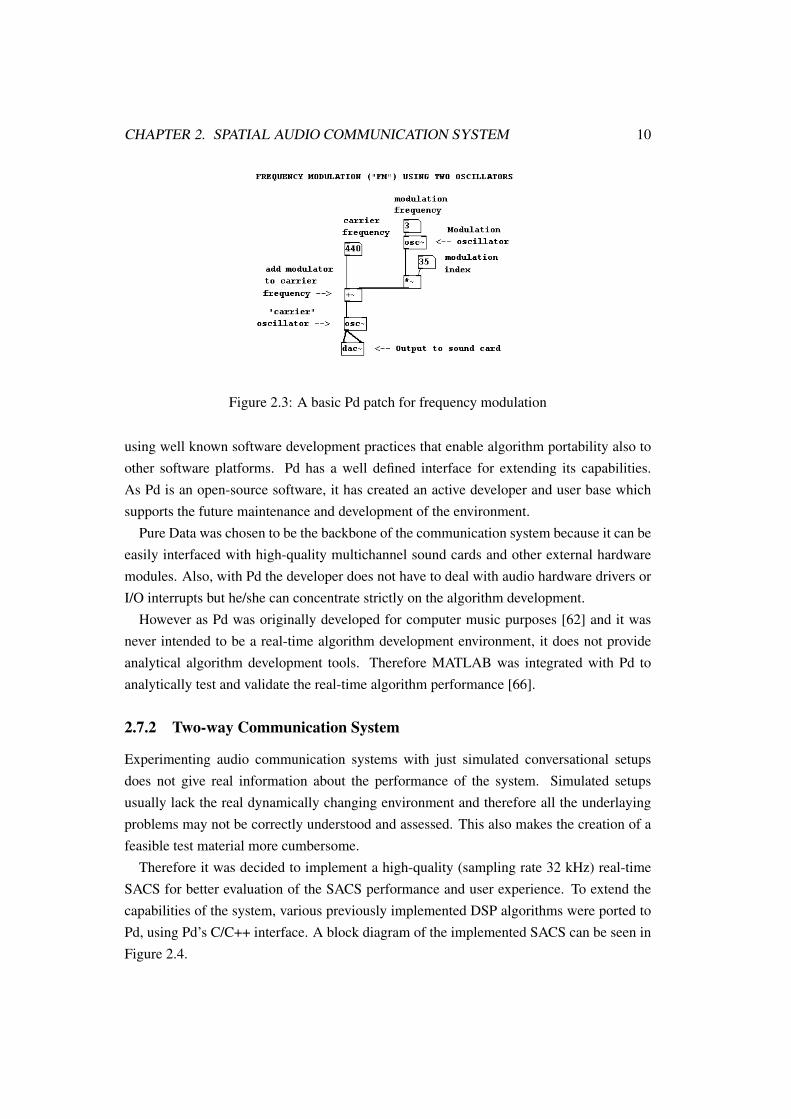
Pure Data can be considered as a graphical programming environment. The startingpoint in Pd is an empty patch or canvas, into which the developer implements the signalprocessing algorithm. The algorithms are developed by using elemental signal processingtasks (e.g. add, multiply, cosine, oscillator) called objects, that are connected to othersignal processing objects with patch cords. By creating networks of these signal processingobjects, complex algorithms can be implemented. An example of and Pd patch can be seenin Figure 2.3 where a simple frequency modulation algorithm is presented.
New signal processing objects or so called Pd externals can also be written in C/C++1http://puredata.info
CHAPTER 2. SPATIAL AUDIO COMMUNICATION SYSTEM 10
Figure 2.3: A basic Pd patch for frequency modulation
using well known software development practices that enable algorithm portability also toother software platforms. Pd has a well defined interface for extending its capabilities.As Pd is an open-source software, it has created an active developer and user base whichsupports the future maintenance and development of the environment.
Pure Data was chosen to be the backbone of the communication system because it can beeasily interfaced with high-quality multichannel sound cards and other external hardwaremodules. Also, with Pd the developer does not have to deal with audio hardware drivers orI/O interrupts but he/she can concentrate strictly on the algorithm development.
However as Pd was originally developed for computer music purposes [62] and it wasnever intended to be a real-time algorithm development environment, it does not provideanalytical algorithm development tools. Therefore MATLAB was integrated with Pd toanalytically test and validate the real-time algorithm performance [66].
2.7.2 Two-way Communication System
Experimenting audio communication systems with just simulated conversational setupsdoes not give real information about the performance of the system. Simulated setupsusually lack the real dynamically changing environment and therefore all the underlayingproblems may not be correctly understood and assessed. This also makes the creation of afeasible test material more cumbersome.
Therefore it was decided to implement a high-quality (sampling rate 32 kHz) real-timeSACS for better evaluation of the SACS performance and user experience. To extend thecapabilities of the system, various previously implemented DSP algorithms were ported toPd, using Pd’s C/C++ interface. A block diagram of the implemented SACS can be seen inFigure 2.4.

CHAPTER 2. SPATIAL AUDIO COMMUNICATION SYSTEM 11
Figure 2.4: The block diagram of the implemented communication system
As can be seen from the block diagram, various capture and rendering methods havebeen implemented. The audio capture can be done in single-channel mono format or withthe Distributed Microphone Array System (DMAS) presented in Chapter 3. Similarly, audiorendering can be done in single-channel format and two different spatial rendering methodshave been implemented. Binaural rendering is intended for headphone use but can also beused for closely placed loudspeakers. For multiple loudspeakers, Vector Base AmplitudePanning (VBAP) can be used as a rendering method.
The communication is done by transmitting single-channel audio stream over IP net-work. The audio transfer is based on netsend∼/netreceive∼ [3] Pd externals made by OlafMatthes. These externals enable the multichannel transfer of raw audio data using TCP andUDP. While TCP causes more latency to the end-to-end connection than UDP, in experi-ments it has been noted that in this audio transfer implementation TCP protocol providesmore robust audio data transfer in the current network environment. Also, to reduce the re-quired network bandwidth the externals were modified to support audio transfers using ansuper-wideband audio codec. The audio codec can be configured for low bandwidth situa-tion by decreasing the data bitrate at the expense of audio quality. A video feed transmissionwas also implemented using Graphics Environment for Multimedia (GEM) extension for Pdand H.264 video codec.

CHAPTER 2. SPATIAL AUDIO COMMUNICATION SYSTEM 12
2.7.3 Wide-band Acoustic Echo Control
As stated in Chapter 2, echo cancellation is essential for good SACS performance. For thisSACS implementation a single-channel adaptive echo cancellation algorithm described in[55] was ported to Pd as a Pd external. However, because the sampling rate of the SACSwas set to 32 kHz, an extremely long adaptive filter would have been required for sufficientecho attenuation. Therefore, a hybrid echo canceller was implemented as suggested inChapter 2.3.
As shown in Figure 2.5 the hybrid echo canceller/suppressor was implemented by firstdividing the input signal to two sub-bands of 0 - 8 kHz and 8 - 16 kHz. To further reduce thelength of the required adaptive filter, the lower sub-band was still divided to two sub-bandsof 0 - 4 kHz and 4 - 8 kHz. The adaptive filtering was used only for the lowest sub-band andsuppression was used for the higher sub-bands. Previously implemented Quadrature MirrorFilter (QMF) [76] was ported to Pd and used to filter the signal to sub-bands.
Figure 2.5: The hybrid adaptive echo cancellation/suppression
However, the use of QMF to filter the signals is not optimal for hybrid echo cancella-tion/suppression [30]. In QMF the bandpass filters overlap in the transition band in order tohave minimal attenuation in all the frequency band. This overlap also extends the cutoff fre-quency of the bandpass filters and therefore the sub-band signals are not strictly bandlimitedto half sampling rate. During the downsampling this causes aliasing in the transition band.This property of QMFs deteriorates the AEC performance as can be seen from Figure 2.6,

CHAPTER 2. SPATIAL AUDIO COMMUNICATION SYSTEM 13
where in Figure 2.6(a) the echo is not attenuated from the transition bands. Figure 2.6(b)shows a spectrogram of a full-band AEC with the same filter length as in left image. Infull-band AEC, filtering is used for the whole bandwidth.
(a) Hybrid AEC and RES (b) Full band AEC
Figure 2.6: Spectrogram of the outputs of hybrid AEC and full band AEC. Input signal iswhite Gaussian noise.
The echo cancellation was placed after the DMAS for computational purposes. In [40]Hämäläinen and Myllylä compare different echo cancellation and beamformer integrationschemas. In their paper they conclude that when echo cancellation is placed after the beam-former (so called ’AEC-last’ configuration), the AEC performance deteriorates rapidlywhen even small changes occur in the steering direction of the beamformer. Thereforethey suggest an ’AEC-middle’ configuration, where the AEC is placed between the PBFpre-filter and the post-filter. However, due to the computational limitations this can not bedone in real-time in the implemented SACS. Similar AEC and microphone array integrationstrategies are also proposed by Kellermann in [46].
However, the main objective of this work is presented in the following chapters, wherethe theory and evaluation of a Distributed Microphone Array System (DMAS) is described.The goal of the proposed DMAS design is to function as an audio capture front-end in theexperimental audio communication platform described in this chapter.

Chapter 3
Microphone Array Techniques
In this Chapter the microphone array techniques for a Spatial Audio Communication Sys-tem (SACS) front-end are described. In Chapter 3.1 theory of beamforming is reviewedand more detailed description of Polynomial Beamformer (PBF) is given. After that inChapter 3.2 a framework for speech source Direction Of Arrival (DOA) estimation basedon beamforming is presented. Finally in the last Chapter 3.3, the data fusion from severalmicrophone arrays is discussed and a method for distributed speech source localization ispresented.
3.1 Beamforming
In beamforming the directivity of a sensor array is altered in order to maximize the arraysensitivity to the direction of the desired source while at the same time minimizing the arraysensitivity in the direction of interfering noise sources. It can also be considered as spatialfiltering where signals are separated by their physical location.
In the following, first an introduction to beamforming techniques is given in 3.1.1. Next,a review of the basic beamforming theory is given in Chapter 3.1.2 and measures for beam-former evaluation are presented in Chapter 3.1.3. Finally, the theory of Polynomial Beam-former (PBF) structure for continuous beam steering is described in Chapter 3.1.4.
3.1.1 Background
In general, beamforming techniques are widely used in antenna, sonar and radar applica-tions. In principle, the idea in beamforming is to place FIR filters in each sensor channelthus enabling spatial and temporal control over the beamformer response. Beamformingtechniques can be divided between data independent [83] and data dependent [79] beam-forming. In data independent beamforming the signal processing is not dependent on the
14
CHAPTER 3. MICROPHONE ARRAY TECHNIQUES 15
statistics of the sensor data whereas in data dependent beamforming the estimated statisticsof the sensor data it taken into account when optimizing the array response.
The first applications of the data independent beamforming techniques to wideband speechsignals were made by Flanagan et al. [29], where they introduced a beamforming techniqueand microphone array design criteria for large auditoriums. However, their design was onlyeffective for narrow band signals and therefore various generalizations to wideband signalshave been proposed e.g in [19, 28, 81].
Most data dependent beamformer designs are based on so called Minimum Mean SquareError (MMSE) design or Linearly Constrained Minimum Variance (LCMV) design. MMSEbeamformer design is based on minimizing the Mean Square Error (MSE) between desiredresponse and the actual response of the beamformer. The main problem with MMSE designis that it requires estimates separately for the interference signal and the source signal cross-correlations, which in general can be difficult to estimate. Also, MMSE design does notguarantee undistorted output signal [36, 72].
In LCMV design the estimation of the desired signal is avoided by using the estimate ofthe overall microphone signal cross-correlations and imposing constraints on the estimatedposition of the desired source signal. The beamformer response can be derived by mini-mizing the beamformer output variance subject to the constraints. The most widely usedLCMV beamforming techniques are based on the so called Generalized Sidelobe Canceller(GSC) that was introduced by Griffiths and Jim [31]. Various extensions and improvementsto GSC have been proposed e.g in [35, 37].
Although GSC based beamformers perform well if the direction of the desired sourceis known, they are not suitable for situations where several source directions have to betaken into account. This is because the constraints are dependent on a priori known sourcelocations. Also, slow convergence of the adaptive filtering used in most of the GSC basedbeamformers makes the beamformer response unpredictable in dynamically changing envi-ronments. Furthermore, in this work the beamformer output is used for speaker localization,which makes the use of data dependent beamforming unpractical. Therefore here the inter-est is in data independent beamformers and especially in Polynomial Beamformer (PBF)which parameterizes the beamformer FIR filter coefficients and thus enables continuousbeam steering.
3.1.2 Basic Beamforming Theory
Consider a point source S at location ps = [ps,xps,yps,z] radiating harmonic spherical pres-sure waves in a lossless (no turbulence or temperature changes) and noisy environment. Anarbitrary microphone array of M ideal omnidirectional microphones measures the pressurewave at pm = [pm,x pm,y pm,z], where m = [1, 2, . . . ,M ]. In this work it is assumed

CHAPTER 3. MICROPHONE ARRAY TECHNIQUES 16
that the Euclidean distance between ps and pm is long enough in order to approximate thepressure wave with a plane wave. The output of mth microphone in discrete time domain is
xm(n) = sm(n) + ϑm(n), (3.1)
where sm(n) is the source signal as captured by themth microphone and ϑm(n) is the noisesignal in themth microphone. The source signal and the noise signal are assumed to be zeromean and uncorrelated.
Figure 3.1: A basic beamformer structure
A basic filter-and-sum beamformer structure is shown in Figure 3.1. Thus, the output ofthe beamformer can be written as
y(n) =M∑m=1
L−1∑k=0
hm(k)xm(n− k), (3.2)
where hm(k) is the impulse response of themth beamforming filter and L is the filter length.In the most trivial case the filters hm(k) can be just delays. In this case, the delays areadjusted so that the phase of the source signal is aligned to be the same at each microphonelocation. The output of this so called Delay-and-Sum Beamformer (DSB) [42] is
y(n) =M∑m=1
xm(n− τm), (3.3)
where τm = (|ps − pm| − |ps − p1|)/c.The main problem with DSB is that the output beam pattern is frequency dependent. In
high frequencies the beam is narrower than in the low frequencies. In low frequencies thewavelength is larger, thus resulting in a wider beam. This is demonstrated in Figure 3.2

CHAPTER 3. MICROPHONE ARRAY TECHNIQUES 17
where a response of a equally-spaced linear delay-and-sum beamformer steered to the end-fire [20] steering direction is shown. In the figure also a phenomenon called spatial aliasingcan be seen in the high frequencies. Spatial aliasing is similar as temporal aliasing, whereduring sampling, the frequency components over Nyquist frequency, i.e. half sampling rate,are folded back to the desired frequency band. Similarly, spatial aliasing occurs if the inter-sensor spacing is larger than half wavelength of the highest frequency in the beamformerdesign bandwidth.
Figure 3.2: Response of a delay-and-sum beamformer.
In order to improve the DSB directivity and the frequency independence of the beampattern, various methods have been suggested. For example a microphone array can be cre-ated by nesting several equally-spaced linear subarrays with different inter-sensor spacings,and using each subarray only for desired narrow-band frequency range. With this so calledharmonic nesting constant beamwidth for wide bandwidth can be achieved, by combiningthe output of each subarray. This approach has been used e.g in [28] and in [19], whereFIR filters are also used to control the frequency variations inside each subarray. By usingunequally-spaced array and FIR low-pass filters a constant beamwidth for entire spatial re-gion can be created as demonstrated by Ward et al. in [81, 82]. In their microphone arrayand beamformer design method, Ward et al. use low-pass filters to control the effectiveaperture size of an unequally-spaced linear array.

CHAPTER 3. MICROPHONE ARRAY TECHNIQUES 18
3.1.3 Beamformer Evaluation
To compare different beamformer designs, different performance measures have been de-veloped. These measures include array gain, beampattern, directivity index and outputpower [11].
The most obvious reason for using an array of microphones instead of just one micro-phone is to improve the signal-to-noise ratio (SNR) of the output signal. This quality canbe measured with array gain that can be formulated as:
G =SNRarraySNRsensor
, (3.4)
where SNRarray refers to the signal-to-noise ratio at the output of the microphone arrayand SNRsensor is the signal-to-noise ratio in the output of just one sensor.
Beampattern or the beamformer spatial-temporal transfer function gives the beamformerresponse to a wavefront coming from a specific direction and specific frequency. An ex-ample of beamformer beampattern can be seen in Figure 3.2. It also should be noted that,in general 3D setup where the beampattern depends on azimuth and elevation angles, thebeampattern can not be plotted in one single plot.
Output power is the measure of - as the name suggests - the total output power of thebeamformer. This can be obtained from the beampattern by summing the beampattern overall the frequencies.
Directivity index is used to measure how well the beamformer suppresses signals fromother directions compared to the steering direction. If |H(ω, θ, φ)|2 is used to denote thepower spectrum of the beamformer as the function of frequency ω and azimuth θ and ele-vation φ angles, the directivity of the beamformer is
DI(ω) = 10 log10
|H(ω, θ, φ)|2
14π
∫ π
0
∫ 2π
0|H(ω, θ, φ)|2 sin(φ)dθdφ
. (3.5)
Other measures to analyze beamformer performance also exist but are not discussed here infurther detail. For a short description of these measures, the reader is advised to take lookat [11].
3.1.4 Polynomial Beamformer
Essentially Polynomial Beamformer (PBF) [40, 44] is a filter-and-sum beamformer withadjustable filter characteristics. In PBF the FIR filter coefficients are approximated by usinga polynomial function basis. The PBF approximation method is based on the well known

CHAPTER 3. MICROPHONE ARRAY TECHNIQUES 19
Farrow structure [27], where Taylor polynomials are used for continuous delay control invariable digital delay line. In the following the PBF filter structure is shortly reviewed.
To steer a filter-and-sum beamformer to multiple desired look directions Di, where i =[1, 2, . . . , ND] and Di defines both azimuth and elevation angles, M×ND FIR filters haveto be optimized. Thus, the output of the beamformer (3.2) becomes
y(n,Di) =M∑m=1
L−1∑k=0
hm,k(Di)xm(n− k). (3.6)
In PBF the FIR filters are approximated as polynomial functions of order P
hm,k(Di) = F0(Di)a0(m, k) + F1(Di)a1(m, k) + . . .+ FP (Di)aP (m, k), (3.7)
where FP is a scalar function of the continuous steering parameter Di. When FP is chosento be a Taylor polynomial, equation (3.7) is equivalent with the Farrow filter structure.
By inserting hm,k(Di) from equation (3.7) to (3.6), the output of PBF can be written as
y(n,Di) =M∑m=1
L−1∑k=0
P∑p=0
Fp(Di)ap(m, k)xm(n− k), (3.8)
and by reordering the terms, the output of the PBF comes
y(n,Di) =P∑p=0
Fp(Di)M∑m=1
L−1∑k=0
ap(m, k)xm(n− k). (3.9)
From (3.9) it can be seen that the PBF filter structure can be divided into two parts: thepre-filter and the post-filter. The pre-filter can be defined as
y′p(n) =M∑m=1
L−1∑k=0
ap(m, k)xm(n− k) (3.10)
and it creates P fixed intermediate beams. The post-filter
y(n,Di) =P∑p=0
Fp(Di)y′p(n) (3.11)
is then used to dynamically steer the intermediate beams to the desired look directionsas shown in Figure 3.3. Because the post-filter calculations can be done very efficientlythe PBF structure enables an easy way to create a desired number of parallel beams bycontrolling just one (2D) or two (3D) parameters. More detailed analysis of the computa-tional performance and also a comparison with traditional filter-and-sum beamformer canbe found in [44] and a PBF implemented as a GSC beamformer structure is presented in[56].

CHAPTER 3. MICROPHONE ARRAY TECHNIQUES 20
Figure 3.3: The Polynomial Beamformer (PBF) structure
The optimization of the pre-filter coefficients ap(m, k) is done by defining Ωd desiredsource signal locations and Ωn interference source locations. Next, ΩS = Ωd∪Ωn definesall the source positions and Ωφ defines the beamformer look directions. Now the MeanSquare Error (MSE) between desired PBF output response and the actual response is definedas
eMSE =∑S∈Ωs
∑f∈Ωf
∑D∈Ωφ
(|Y (z,D)| − |Y (z,D)|)2
|ΩS | · |Ωf | · |Ωφ|, (3.12)
where Ωf defines the frequencies and Y (z,D) and Y (z,D) are the beamformer outputsin the frequency domain for the desired output response and the actual output responserespectively. The pre-filter coefficients are optimized by minimizing the MSE function[43, 44].
3.2 Direction of Arrival Estimation
The goal of sound source localization algorithms is to estimate the source position of theincident sound wave captured by a microphone array. Most common sound source local-ization methods are based on the Time Difference of Arrival (TDOA) of the sound wavealthough other methods also exist. In most of the TDOA algorithms the delay between areference microphone and another microphone in the array is estimated by using Gener-alized Cross Correlation (GCC), where an inverse Fourier transform of a weighted crosscorrelation spectrum between microphone pairs is calculated [17]. Various techniques havebeen proposed to estimate the sound source location from the TDOA estimates [18, 38, 84]
However, the sound source location can not only be estimated by TDOA but also bymeasuring the signal amplitudes or energies. Usually the energy-based sound source local-ization methods are based on the well known phenomenon that the intensity of a acousticwave is inversely proportional to the squared distance. Some localization techniques thatuse this phenomenon are presented in [10, 69].

CHAPTER 3. MICROPHONE ARRAY TECHNIQUES 21
This Chapter starts with a theoretical discussion of the speech source localization frame-work in Chapter 3.2.1. In Chapter 3.2.2 a noise power estimation method is presented thatis necessary when the direction of the beam with the largest SNR is desired. Finally, inChapter 3.2.3 the creation of Spatial Likelihood Function (SLF) from the framework datais described.
3.2.1 Beamformer Based Speaker Localization Framework
In this work the sound source location is estimated by using steerable beamforming. Aa similar approach as was proposed by Kellermann in [45]. The presented localizationalgorithm is based on [77] and it uses the PBF structure to generate a set of beams fromwhich the beam with the largest signal power is defined. The Direction Of Arrival (DOA)of the sound source is then estimated to be in the steering direction of that beam. Finally,also the range of the sound source can be estimated by fusing the multiple DOA estimatesproduced by multiple microphone arrays.
When using a steerable beamformer the straightforward manner to estimate the dominantspeaker direction is to find the beam with the largest signal power. However, especially inlow Signal-to-Noise Ratio (SNR) conditions, for example inside a car, it is more beneficialto find the beam with the largest SNR than the beam with largest signal power. But ingeneral the beam with largest SNR is not steered to the direction of active speaker. Forexample if the noise source is in the same direction as the speaker, it is not likely that thebeam steered to that direction has the largest SNR. As the proposed system is intendedfor office use where generally the SNR is high, it is more likely that the speaker is at thesteering direction of the beam with highest signal power. However, in the following bothcases are considered.
As in the previous chapter let us consider that a beamformer output consists ofND beamssteered to (θi, φi) directions, where i = [1, 2, . . . , ND]. Now the output of the ith beam ofthe PBF can be written as
y(n,Di) =P∑p=0
Fp(Di)M∑m=1
L−1∑k=0
[ap(m, k)sm(n− k) + ap(m, k)ϑm(n− k)]
=P∑p=0
Fp(Di)M∑m=1
L−1∑k=0
ap(m, k)sm(n− k)
+P∑p=0
Fp(Di)M∑m=1
L−1∑k=0
ap(m, k)vm(n− k)
= ys(n,Di) + yϑ(n,Di). (3.13)
From equation (3.13) it can be seen that the source signal and the noise signal still have

CHAPTER 3. MICROPHONE ARRAY TECHNIQUES 22
a simple additive relation and are uncorrelated in each beam if sm(n) and ϑm(n) also areuncorrelated.
When the speech and noise signals are uncorrelated the total signal power of the ith beambecomes
Ws(n,Di) = E|y(n,Di)|2 = E|ys(n,Di) + yϑ(n,Di)|2
= Eys(n,Di)2+ 2Eys(n,Di)yϑ(n,Di)︸ ︷︷ ︸=0
+Eyϑ(n,Di)2
= Eys(n,Di)2+ Eyϑ(n,Di)2. (3.14)
When the signal power estimate of the ith beam in equation (3.14) is divided by the noisepower, we have
Wr(n,Di) =E|y(n,Di)|2Eyϑ(n,Di)2
=Eys(n,Di)2Eyϑ(n,Di)2
+ 1. (3.15)
As can be seen from equation (3.15), Wr(n,Di) is proportional to the SNR of the ith
beam, while Ws(n,Di) gives the total output power of the ith beam. Now a choice canbe made as to what quantity will be used for speech source DOA estimation. In generalthe choice depends on the acoustical environment and the actual application where speakerlocalization is utilized but based on our experimentation it can be said that if the microphoneoutput signal SNR is low, then Wr will give better results than Ws, which leads to beamlevel estimate,
W (n,Di) =
Ws(n,Di), if SNR > δ dBWr(n,Di), otherwise
(3.16)
where δ is a SNR threshold value. However additional work has to be done in order todetermine the desired value of δ.
Also, to make the DOA estimation more robust against rapid changes in acoustic powerthe beam level estimate is averaged over time instead of calculating the instantaneous beamlevel. The averaging is done by smoothing the beam level estimate with a first-order recur-sive system
P (n,Di) = βP (n− 1,Di) + (1− β)W (n,Di). (3.17)
For sufficient smoothing, the smoothing constant β should be set to values between β =[0.90...0.95] and a step size between [30ms− 70ms] should be used.
This information can be used in finding the DOA of speech signal by calculatingP (n,Di)of each beam and finding its largest value. However, since the absolute value of the beamlevel is not necessary for the localization algorithm and to make the previous beam levels

CHAPTER 3. MICROPHONE ARRAY TECHNIQUES 23
Figure 3.4: The speech tracker
also comparable the beam level estimate of each beam is normalized with the average beamlevel. Now we have
Pavg(n,Di) = NDP (n,Di)∑ND−1
i=0 P (n,Di). (3.18)
Finally, the normalized beam level estimates Pavg(n,Di) have to be compared in orderto find the beam B with the highest beam level P (n)
B = arg maxDi
Pavg(n,Di) (3.19)
P (n) = Pavg(n,B) (3.20)
and thus also the estimate for the speech source direction. However, when tracking aspeaker in a two-way communication system the tracking should be done only during thenear-end speech activity and the far-end speech pauses. Therefore a voice activity detector(VAD), such as [52], is needed for robust speaker tracking. In here the voice activities areassumed to be known.
Thus, during the far-end speech pause and near-end speech activity, first the beam withthe highest normalized beam level P (n) is calculated. Then a decision of a new speaker di-rection is made by comparing the relative level difference betweenPavg(n,B) andPavg(n−1,B) to a threshold value γ. The new speaker direction is decided by,
D(n) =
B, if Pavg(n,B)
Pavg(n−1,B) > γ
D(n− 1), otherwise(3.21)

CHAPTER 3. MICROPHONE ARRAY TECHNIQUES 24
The threshold value γ can be chosen freely but the choice depends on the overall SNR.In low SNR conditions the possible dynamic range is reduced, which suggests the use oflower values of γ. However, experience has show that values near 1 dB provide satisfactoryresults in high SNR conditions. A block diagram of the presented tracking system can befound from Figure 3.4.
3.2.2 Noise Power Estimation
When using Wr as the beam level estimate the critical part of the localization algorithm isthe estimation of the noise power that is needed for successful estimation of the SNRs ofeach beam. The obvious way to estimate the noise power is to calculate the total signalpower when speech is not present i.e during a speech pause. This approach however re-quires a VAD whose performance can be unpredictable especially in low SNR conditionsor in non-stationary noise. Therefore during false speech pause detection the noise powerestimate can have very large variance. As already stated before, the speaker localizationrequires a VAD for robust speaker localization, which suggests that the noise power estima-tion can also be done using the VAD approach. However, the robustness requirements forVAD in power comparison phase of the tracker and in the noise estimation deviate largely.The false activity detection in power comparison does not cause large deterioration in thetracker performance but this is not the case in noise power estimation.
Therefore an algorithm for noise power estimation that does not require VAD is presentedhere. The described noise power estimation method is based on the minimum statisticsapproach by Rainer Martin [50, 51]. In minimum statistics the noise power spectrum isestimated by tracking the minimum value of a smoothed power spectrum of the signalinside a sufficiently long search window. This minimum value gives a biased noise powerestimate for each frequency bin. By analyzing the statistics of the minimum value noisepower estimator, the mean of the estimate can be found and it can be used to produce anunbiased estimate of the noise power.
However, because in the speaker localization framework only the beam’s SNR relative toSNR of other beams is of interest, the unbiased estimate of the noise power is not needed.Also, instead of the power spectrum, the noise power in the full frequency band is estimated.Before search for the minimum value the signal power estimate can also be smoothed sim-ilarly as in equation (3.17) and we get
Es(n,Di) = α(n,Di)Es(n− 1,Di) + [1− α(n,Di)]Ws(n,Di), (3.22)
where α(n,Di) is an adaptive smoothing parameter. In the most trivial case α(n,Di) canbe a constant. Finally, a biased noise power estimator can be formulated as
σ2n(n,Di) = minEs(n,Di), Es(n− 1,Di), ... , Es(n−Q+ 1,Di), (3.23)

CHAPTER 3. MICROPHONE ARRAY TECHNIQUES 25
where Q defines the length of the search window.
Figure 3.5: Noise power estimates. Red: instantaneous signal power, Blue: smoothedsignal power α(n,Di) = 0.90, Black: minimum tracked noise power estimate, searchwindow length Q = 96.
In Figure 3.5 a minimum tracked noise power estimate is shown. In the left figure thenoise power is estimated from the smoothed signal power and in the right figure there is nosmoothing. As can be seen from Figure 3.5, the smoothing widens the power peaks duringspeech activity and therefore causes inaccurate noise power estimates. On the other handif the smoothing is omitted from the signal power computation, also the inaccuracy due tothe wide power peaks is avoided, but instead the variance of the noise power estimate isincreased and the estimate is more biased as can be seen from the left figure. However,this can be avoided by using adaptive smoothing parameter as suggested in [51]. The opti-mal smoothing parameter can be derived by assuming a speech pause and minimizing theconditional mean square error
NMSE(n,Di) = minE[(Es(n,Di)− σ2
n)2|Es(n− 1,Di)], (3.24)
where E is the expectation operator.This leads to the optimal smoothing parameter
αopt(n,Di) =1
1 +(Es(n− 1,Di)σ2n(n,Di)
− 1)2 (3.25)
As can be seen from equation (3.25) the smoothing parameter should be adapted so thatthe value of the parameter is close to one during speech pause and close to zero during

CHAPTER 3. MICROPHONE ARRAY TECHNIQUES 26
speech activity. The detailed derivation of the optimal smoothing parameter as well as itspractical estimation can be found in [51]. Minimum tracker noise power estimate withadaptive smoothing parameter is shown in Figure 3.6.
Figure 3.6: Noise power estimation with adaptive smoothing parameter
3.2.3 Spatial Likelihood Function
As described in Chapter 3.2.1, speaker localization framework gives an estimate for themost likely speaker direction, but in many cases it is also useful to analyze the likelihoodof other speaker directions [5]. This is especially useful when fusing data from severalindividual estimations. The Spatial Likelihood Function (SLF) [5] or Spatial Responseessentially describes a probability Pr(φ(p)|x), where φ(p) is the event that the speakeris located at point p and x is a vector containing the input data of all the microphones.Therefore Pr(φ(p)|x) can be thought as a a posteriori probability for a sound source tolocate in point p in space. However, generally the absolute value of SLF can be difficult tomeasure and therefore there exist methods for measuring
SLF (p) = (ψ(Pr(p)), (3.26)
where ψ(·) is a monotonically non-decreasing function. Using ψ(·) does not impose furtherproblems, because only the relative values of SLF at different source directions or locations

CHAPTER 3. MICROPHONE ARRAY TECHNIQUES 27
are of interest and using monotonically non-decreasing function does not violate the com-parison of these values. In this work whenever likelihood or SLF is referred it is related tolikelihood as defined in equation (3.26).
For the energy-based localization framework the SLF is produced by mapping the valuesof Pavg(n,Di) to the corresponding directions. This can be formulated so that first theazimuth and elevation angles for each possible source location p relative to array at pm arecalculated as
θx,y,z = arctan[py−pm,ypx−pm,x
]φx,y,z = arctan
[pz−pm,z√
(px−pm,x)2+(py−pm,y)2
].
(3.27)
Next, all possible source points ps in space that are included in the area covered bysteering direction (Di) are given a value Pavg(n,Di), i.e.
SLF (n,p) =
Pavg(n,Di), if
θx,y,z −∆θ ≤ θi < φx,y,z + ∆θ
∧φx,y,z −∆φ ≤ φi < φx,y,z + ∆φ
0, otherwise
(3.28)
where (θi, φi) are the steering angles of the ith beam and ∆θ, ∆φ are tolerance parametersthat define the beam width in SLF calculations. For example when the steering directionsare equally spaced in azimuth plane, the tolerance parameter can be calculated as: 2∆θ =2π/Nθ, where Nθ is the number of beams in the azimuth plane. However, it is not obviousthat SLF (n,p) can be used as an estimate for the likelihood function but this can be provensimilarly as cross-correlation based SLF is proven in [5].
Essentially SLF (n,p) is an observational estimate of Pr(x|φ(p)), which describes theprobability of the input data to be x, in case of an event that the speaker is located at pointp. The relation between Pr(x|φ(p)) and Pr(φ(p)|x) is found with with Bayes’ theoremwhich states that
Pr(φ(p)|x) =Pr(x|φ(p))Pr(φ(p))
Pr(x)(3.29)
From equation (3.29) it can be seen that Pr(x) is not dependent on p and therefore doesnot change the relative values of SLF at different points in space. Also, φ(p) describes thea priori probability for the event that the speaker is located at point p. If it is assumed thatall the possible points in space are possible source locations, φ(p) is constant over p, whichmakes the SLF only a constant scaling of the observational estimate Pr(x|φ(p)).
Figure 3.7 shows an example of an SLF that is produced with tracking framework de-scribed in Chapter 3.2.1. The red line marks the 0 direction and the angle increasesclockwise. Larger values indicate higher speech source likelihood and thus the speakeris estimated to locate at the direction of 130.

CHAPTER 3. MICROPHONE ARRAY TECHNIQUES 28
Figure 3.7: Example of a Spatial Likelihood Function, from recordings with circular mi-crophone array of eight microphones [40].
CHAPTER 3. MICROPHONE ARRAY TECHNIQUES 29
3.3 Distributed Microphone Arrays
In this Chapter few possibilities of distributed signal processing are discussed. In Chap-ter 3.3.1 a short introduction and motivation for distributed signal processing is given. Thefusing of the speech source DOA data of each microphone array in order to obtain thespeech source location estimate is described in Chapter 3.3.2.
3.3.1 Background
As already stated, in beamforming the array sensitivity is increased to the direction of thedesired source, while at the same time noise sources from other directions are attenuated.However, the attenuation of signal energy due to the distance that the acoustic wave travels,decreases the SNR of the microphone array and therefore also the parameter estimationerror increases. An obvious solution for this is to place microphone arrays at differentpoints in a room, thus decreasing the effect of attenuated signal energy. Also, by combiningthe DOA data of each microphone array the direction and/or position of sound source canbe estimated more accurately.
In distributed signal processing each processing unit, e.g. one microphone array, is calleda node. Node is responsible for all the local signal capture and processing. The commu-nication between individual nodes depends of the topology of the sensor network which intheory can change very frequently [7]. One of the most common topologies is so called startopology, where each node sends its data to a master node that combines the data from theindividual nodes and, when necessary, sends the combined data forward. The main prob-lems in distributed audio signal processing, where the sensor topology can be assumed tobe constant, are the transfer and the fusion of the data of each processing node. In this worktransferring the data from node to node is assumed to be perfect, i.e. the internal clocks ofeach node are synchronized with each other, there are no latencies in the transfer, etc.
3.3.2 Sound Source Localization from Multiple DOA Estimates
The fusion of the individual microphone array data can be done in several ways. In [48]Liu et al. estimate the sound source position by finding the intersection of several DOAlines from each microphone array. In the case of non-intersecting lines, the sound sourceposition is defined to be the point that has minimal overall distance from the lines. In idealconditions this method gives optimal sound source position estimate, but errors due to noisesources, inaccurate microphone calibration, etc. can lead to erroneous DOA estimates andtherefore also erroneous sound source position estimate.
Figure 3.8 presents an example of a simulated setup of four microphone arrays, whereeach microphone array consists of 10 ideal cardioid microphones, thus creating cardioid

CHAPTER 3. MICROPHONE ARRAY TECHNIQUES 30
shaped beams in 36 intervals. The DOA estimates for each microphone array are formedby using the localization framework presented in Chapter 3.2.1 and finally the DOA esti-mates are combined by searching the minimal overall distance from the DOA lines. The leftfigure presents conditions with ideal microphone calibration whereas in the right figure themicrophone gains are uniformly distributed between ±0.5 dB. The input signal is Englishfemale speaker. The blue square shows the real speaker position and black star shows theestimated speaker position. The microphone array positions are marked with red circles.
The fusion of DOA data can also be done by using the Spatial Likelihood Function pre-sented in Section 3.2.3. This way also the likelihood of other DOA estimates is taken intoaccount in the sound source position estimation. By using not only the most likely DOAestimate, but also the likelihood of other DOA estimates, the sound source localization canbe made more robust against estimation errors.
The most straightforward way for combining the SLFs of each array is to sum the SLFsof each individual array to form a global estimate of the SLF function as shown in [5]. Nowa global SLF is
SLF (n,p) =1NM
NM∑i=1
SLFi(n,p), (3.30)
where NM is the number of microphone arrays and SLFi(n,p) is the SLF generated bythe ith array. Now the speaker position estimate can found by searching a maximum ofSLF (n,p), i.e.,
p(n) = arg maxpSLF (n,p) (3.31)
However, when SLF is created using the localization framework as presented in Sec-tion 3.2.1, it should be noted that in general there are several source points with the samemaximum value of SLF (n,p). This is due to the finite DOA estimate resolution whichcreates areas with the same SLF values. The final speaker position estimate can be foundas a midpoint of all the points with maximum SLF value
ps(n) =1NP
NP−1∑i=0
pi(n), (3.32)
where NP is the number of points with the same maximum SLF value and pi is the coordi-nates of the ith maximum value.
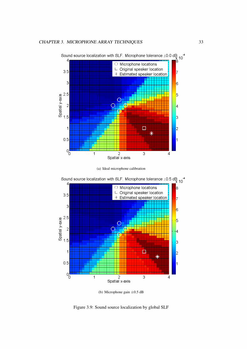
An example of global SLF can be seen in Figure 3.9, where the simulated setup is thesame as in Figure 3.8. Here the sound source position is estimated by using the likelihoodof all DOA estimates and thus forming a global SLF. Similarly as in Figure 3.8, the leftfigure shows the global SLF with ideal microphone calibration and in the right figure themicrophone gains are uniformly distributed between ±0.5 dB. Also as in Figure 3.8, the

CHAPTER 3. MICROPHONE ARRAY TECHNIQUES 31
(a) Ideal microphone calibration
(b) Microphone gain ±0.5 dB
Figure 3.8: Sound source localization by searching the point with minimal overall distancefrom several DOA lines.
CHAPTER 3. MICROPHONE ARRAY TECHNIQUES 32
square shows the real speaker position, star shows the estimated speaker position and themicrophone array positions are marked with circles.
As can be seen from Figures 3.8 and 3.9, in some situations the global SLF provides morerobust speaker localization when there are errors in microphone calibration. The search ofsmallest distance can cause large speech source localization estimation errors, when evenone of the individual DOA estimations deviates significantly from DOA estimates of othermicrophone arrays. In the case of global SLF this error is reduced by averaging over allthe DOA estimates from all the microphone arrays. More thorough comparison of the twomethods is presented in Chapter 4.4.2.
Also other methods for generating the global SLF have been proposed. A MaximumLikelihood (ML) estimate of the sound source location by using acoustic energy is presentedin [69] and in [6] ML estimate is formulated by using relative time delays. A different kindof approach is presented in [60] where a kinematic model for speaker state (position andvelocity) is generated and sequential Kalman filtering is used to fuse the state estimates ofeach microphone array.
CHAPTER 3. MICROPHONE ARRAY TECHNIQUES 33
(a) Ideal microphone calibration
(b) Microphone gain ±0.5 dB
Figure 3.9: Sound source localization by global SLF

Chapter 4
Experimentation
In the following chapters the implemented microphone array and its performance is dis-cussed. First in Chapter 4.1, the design of the implemented microphone array and the mo-tivation for the chosen design is discussed. Next, in the Chapter 4.2, the measurements toevaluate the system performance in normal acoustic conditions are presented and the nexttwo Chapters 4.3 and 4.4 discuss the system performance in simulated and in measuredconditions.
4.1 Microphone Array Design
4.1.1 Geometry
In this thesis the interest is in small microphone arrays and therefore it was decided to usejust a few microphones for each microphone array. By restricting the number of micro-phones, also the hardware requirements can be held under control when using multiple mi-crophone arrays. Four microphones was chosen to be an adequate number of microphonesfor each array.
For this work a circular microphone array with one microphone in the center was chosen.This way a microphone array with microphones placed in corners of equilateral triangleand in the circumcenter of the triangle is formed. The radius of the circle with center in thecircumcenter of the triangle was chosen to be 35 mm, which makes the spatial aliasing limitto be approximately 5 kHz. The microphones were placed on top of a chipboard piece andthe resulting microphone array can be seen in Figure 4.1 and the microphone locations areshown in Table 4.1. The final Distributed Microphone Array System (DMAS) presented inthis work uses three of the aforementioned microphone arrays of four microphones. Threemicrophone arrays is sufficient to cover an area of a normal office room while also main-taining the total number of microphones in control.
34

CHAPTER 4. EXPERIMENTATION 35
Figure 4.1: The prototype microphone array
Mic x[mm] y[mm] z[mm]
1 0 0 0
2 35 0 0
3 35cos(2π3 ) 35sin(2π
3 ) 0
4 35cos(−2π3 ) 35sin(−2π
3 ) 0
Table 4.1: Microphone locations in millimeters.

CHAPTER 4. EXPERIMENTATION 36
4.1.2 PBF Design
The PBF filter coefficients can be optimized for arbitrary shaped microphone arrays andwith arbitrary beam steering properties. For this application the PBF was designed for ateleconference-like situation where the speakers are sitting around a table and the micro-phone arrays are placed on top of the table. Therefore it was decided to use fixed steeringangle for elevation while maintaining continuous steering in azimuth plane. The PBF fil-ter coefficients were optimized for elevation angles between 15 and 25. In practice thismeans that if the speaker’s mouth lies 0.5 m above the table surface, the optimum results areachieved when the microphone arrays is 1.07 m - 1.87 m from the speaker. The samplingrate of the PBF was chosen to be 8 kHz and the component tolerance was set to 0.5 dB.
When PBF is used for speaker localization, the most notable error source is the exis-tence of a systematic bias error in the beamformer output power. This is demonstrated inFigure 4.2, where the output power of the PBF is plotted. As can be seen from the Fig-ure 4.2(a) the DOA of the maximum output power is deviated over 10 from the real sourceDOA. This is due to the low order of the PBF polynomial that is used to approximate thebeamformer filter coefficients. In real world situations also microphone calibration errorscan cause systematic error in the PBF output. In Figure 4.2(b) a higher order polynomialis used and the systematic error is reduced significantly. In the figures black star shows theDOA with the highest output power and blue square shows the real DOA.
(a) Order of the PBF polynomial P = 4 (b) Order of the PBF polynomial P = 6
Figure 4.2: The bias error in the PBF output power.
When only one microphone array is used, the bias error does not effect the PBF perfor-mance, because the input signal is always filtered with the beam that provides the largestoutput power. However, when biased PBF outputs from multiple microphone arrays that

CHAPTER 4. EXPERIMENTATION 37
can have different bias errors in different directions are used to track a sound source, thebias errors are also present in the output of the whole distributed microphone array system.This deteriorates the performance of the whole system and therefore it has to be made surethat sufficiently high polynomials are used and that the microphones are calibrated. There-fore in this work, polynomials of order 6 are used to approximate the beamformer filtercoefficients.
4.2 Measurements
A set of measurement were made to experiment and to test the distributed microphone arraysystem and they are described in the following chapters. The measurements were made incollaboration with the Audio Research Group in the Department of Signal Processing inTampere University of Technology (TUT).
4.2.1 Measurement Environment
Measurements were made in a listening room in the TUT audio laboratory. The room alsoincluded table, sofa and several audio equipment. The reverberation time T60 of the roomwas measured to be 0.25 s. Although this reverberation time is lower than in normal officeor living room it is appropriate for testing and validating the system described in this work.The noise level of the room was below the sensitivity of B & K 2232 sound pressure meter.
4.2.2 Hardware
Commercial high quality audio hardware was used in the measurement. The microphoneswere required to be small enough to be suitable for microphone arrays and omnidirectionalso that unwanted attenuation of signal energy does not happen due to the sound sourcelocation. The selected microphones were DPA 4060-BM pre-polarized omnidirectionalminiature condenser microphones [1].
The microphones were connected to a Presonus Firepod microphone pre-amplifier andA/D converter [4], that was run with a desktop PC computer with Windows XP operat-ing system. Cubase recording software was used to capture the microphone signals. Themicrophone signals were sampled using 48 kHz sampling frequency and 32 bits for eachsample. Similarly Adobe Audition was used to play the source signals. The playbackPC used RME-Hammerfall Multiface D/A converter that was connected to four Genelec1029 A loudspeakers [2] for playback.

CHAPTER 4. EXPERIMENTATION 38
4.2.3 The System Geometry
In the measurement setup the microphone arrays were placed to simulate a teleconference-like situation, where all the microphones are on top of a table that is located between thespeakers. Therefore, the microphone array locations were arbitraryly chosen but restrictedto be on the table. The room layout and measurement geometry can be seen in Figure 4.3.
Figure 4.3: The recording setup.
4.2.4 Source Material
Several simulated conversational setups were created by using prerecorded speech samplesfrom the TIMIT speech database. The speech samples include male and female speakersspeaking in English. Also the impulse responses from each loudspeaker to each microphonewere measured by using Farina’s method [26].
4.2.5 Outcome of the Measurements
After the measurements some artifacts were found in the measured signals. Most promi-nently, as can be seen from Figure 4.4, a low frequency noise was present in the measure-ment data. The low frequency interference appears in all the measured data and is mostlikely due to the air conditioning system or other structural properties of the measurementroom. However, the impulse response estimation method is able to push the interferenceout of the final impulse response estimate and therefore the impulse responses are not dete-riorated by the low-frequency noise.
Also, the signals were measured with two different SNR levels. The source signal soundpressure was measured by playing white noise from the loudspeakers and measuring the
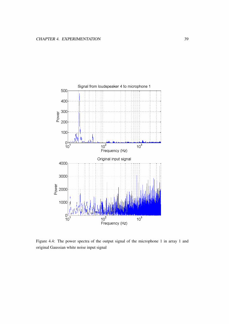
CHAPTER 4. EXPERIMENTATION 39
Figure 4.4: The power spectra of the output signal of the microphone 1 in array 1 andoriginal Gaussian white noise input signal

CHAPTER 4. EXPERIMENTATION 40
sound pressure 30 cm from the loudspeaker. The SNR was modified by changing the outputlevel of the loudspeaker. In high SNR conditions the sound pressure was approximately 81dB and in low SNR conditions the sound pressure was approximately 30 dB lower. Thesound pressure measurements were made A-weighted by using a B & K 2232 sound levelmeter.
No separate microphone calibration measurements were made and therefore the mea-sured impulse responses were used for microphone calibration. The calibration was doneby assuming that all the microphones of one array are placed at location of the array’s centermicrophone and calculating the power of the impulse responses from all the loudspeakers toall the microphones. The impulse response’s powers were averaged over all the loudspeak-ers and finally the gain coefficient for each microphone was defined so that the power ofthe impulse responses is the same at each microphone. However, in reality the microphonesare not located at the same point in space and therefore the used calibration method is notideal. The arrays are located approximately 1.5 m from the loudspeakers, which results inapproximately 0.2 dB error in the microphone calibration, which is under the componenttolerance used in the PBF design.
4.3 PBF Performance
The implemented four-microphone Polynomial Beamformer performance is discussed inthe following chapters. First the PBF performance in simulated setup is presented andfinally performance in real acoustical environment is discussed.
4.3.1 Simulated PBF Performance
The PBF performance is first evaluated by simulating an anechoic environment. The geom-etry of the simulated setup is equivalent with the recording setup and also 48 kHz samplingrate was used in the simulations in order to make the results comparable. The simulationswere made by using a synthesized baseband signal as the microphone input signal. How-ever, the PBF was designed for 8 kHz sampling rate and therefore the microphone signalshad to be downsampled before the PBF processing. The magnitude responses of the originaland downsampled input signals can be seen in Figure 4.5.
When the source is placed at the location of the loudspeaker 4 and the microphone ar-ray 1 (as shown in Figure 4.3) is used to capture the signal, the beam pattern of the fourmicrophone PBF and DSB can be seen in Figure 4.6.
As can be seen from the figure, the PBF design provides significantly more spatial at-tenuation than the DSB. The implemented array aperture is not sufficient for DSB to makeseparation of low frequency signals. The same behavior is also shown in Figure 4.7 where

CHAPTER 4. EXPERIMENTATION 41
(a) Synthesized input signal (b) Input signal after downsampling to 8 kHz
Figure 4.5: Magnitude responses of the input signal.
the directivity and the output power of the PBF and DSB are presented.Figure 4.7(a) emphasizes what already was seen in Figure 4.6, that the PBF provides ap-
proximately 4 dB better directivity than DSB already at 500 Hz. Also in PBF the directivityis constant over wide frequency range. It should be noted that the strange behavior in direc-tivity near 4 kHz is not because of imperfections in the beamformer design but is due to theimperfect anti-aliasing filtering during downsampling. The output powers in Figure 4.7(b)show that with PBF, a sidelobe attenuation of approximately 7 dB can be achieved whereaswith DSB the sidelobe attenuation is only 3 dB. Also, PBF gives 10 dB more of maximumattenuation (difference between maximum and minimum) than DBF. The beam pattern andthe output power are normalized with the output power of the microphone 1 that is locatedat the phase center of the array.
4.3.2 Measured PBF Performance
The PBF performance in real acoustic environment was evaluated by doing measurementsthat are described in Chapter 4.2. It has to be noted that most of the beamformer perfor-mance measures are not well-defined in multi-path propagation conditions and thereforethey can not be used to evaluate the beamformer performance. However some observationcan be made by looking at the directivity and total output power of the beamformer.
Figure 4.8 shows the total output power and the directivity of the PBF (blue) and DSB(red), when the source is played from loudspeaker 4 and captured with microphone array 1.The measured impulse response of the signal path from the loudspeaker to each microphoneis used as the PBF input signal. The output powers are normalized with the output powerof the microphone 1.
As can be seen from Figure 4.8(b), the PBF maximum attenuation is approximately 2.5dB more than with DSB, but also PBF reduces the signal power almost 2 dB compared to

CHAPTER 4. EXPERIMENTATION 42
(a) PBF beam pattern, steered towards loudspeaker 4 from microphone array 1
(b) DSB beam pattern, steered towards loudspeaker 4 from microphone array 1
Figure 4.6: Beam patterns of the implemented microphone array used as PBF and DSB.

CHAPTER 4. EXPERIMENTATION 43
(a) PBF and DBF directivity index (b) PBF and DBF output power
Figure 4.7: Directivity and output power of PBF and DSB.
omnidirectional signal. Compared to the simulated setup, the dynamic range of the PBFoutput power is extensively reduced in real acoustic environment as can be expected.
The measured directivity in room environment in Figure 4.8(a) shows the same kind ofbehavior as in simulated case but now the directivity is deteriorated by the room properties.From the figure it can be noted that at low frequencies DSB can not separate the signals fromdifferent directions at all, while PBF has 3 dB directivity at 300 Hz. But at the same timelarge dips in the measured directivity can be seen at approximately 400, 500 and 600 Hz,which most likely are due to the room resonances in the measurement room. The outcomeis that at these frequencies PBF output power is larger at other directions than the soundsource direction.
However, when speech signal is used as the PBF input signal, i.e. the PBF output isweighted with speech spectrum, the PBF performance is increased when compared to DSB.This is demonstrated in Figure 4.9. As it can be seen from the figure, DSB does not attenuatespeech signal arriving from different directions. This is because the small aperture of themicrophone array causes the directivity of the DSB to be zero over wide frequency rangeas shown in Figure 4.7(a) while at the same time speech signals do not have much powerin the high frequencies where DSB can discriminate with signals arriving from differentdirections.

CHAPTER 4. EXPERIMENTATION 44
(a) PBF and DBF measured directivity in multi-path propagating environment
(b) PBF and DBF measured output power
Figure 4.8: Measured output power and directivity of PBF and DSB.
Figure 4.9: Measured output power of PBF and DSB weighted with speech spectrum.

CHAPTER 4. EXPERIMENTATION 45
4.4 Speech Source Localization Performance
Here the presented speech source localization framework is evaluated first by simulationsand then with measured data.
4.4.1 Noise Power Estimation
When sound source localization is done in low SNR conditions it might be useful to usethe beam with the best SNR as a speech source DOA estimate instead of the beam withthe highest power. This may result in inaccurate DOA estimation but on the other handwhen the DOA estimate is used to steer a beamformer the final beamformer output willhave better SNR. When the desired signal and the noise are zero-mean and uncorrelated theSNR can be estimated with:
SNR = 10 log10
(Ey(n)2Eϑ(n)2
− 1), (4.1)
where y(n) is the desired signal contaminated with noise ϑ(n) and E is the expectationoperator. As it can be seen from equation (4.1) the difficulty in SNR estimation is theestimation of the noise power.
The minimum statistics noise power estimation method presented in Chapter 3.2.2 wasevaluated by using a speech signal of English speaking female as a desired signal and addingwhite Gaussian noise to the desired signal. As the noise power estimation was done sep-arately for each audio frame (length 256 samples) the final noise power estimate was cal-culated by averaging over the noise power estimates of all the frames. Figures 4.10(a) and4.10(b) show the noise power estimate and the SNR estimate, respectively.
The figures show that at very low noise power levels the estimation saturates and there-fore is not anymore reliable. However, between SNR -5 dB to 40 dB the presented noisepower estimation method gives good results. Because the noise power estimation is not themain point of this work the evaluation or the method is done only for stationary white noise.With different type of noises the noise power estimator performs differently and thereforeany generalizations can not be made. A more detailed evaluation of a similar noise powerestimation method is given in [51].
4.4.2 Simulated Source Localization Performance
One array
In far-field the Direction Of Arrival (DOA) of the sound source can be estimated, when onlyone microphone array is used. Here, the DOA estimation method descried in Chapter 3.2and Time Difference of Arrival (TDOA) based DOA estimation method are compared by

CHAPTER 4. EXPERIMENTATION 46
(a) The noise power estimation (b) The SNR estimation
Figure 4.10: Noise power and SNR estimation
simulating anechoic environment in a noise field. The TDOA method used is described in[88], where the least squares solution of the DOA is calculated with estimated time delays.The time delays are estimated by using cross-correlation between the microphone signalsand finding its maximum value.
The first set of simulations are done by using a speech sample of English speaking fe-male as the microphone input signal and placing uncorrelated Gaussian white noise sourcesat 10 intervals around the room shown in 4.3. All the signals are sampled at 48 kHz. Thedelayed microphone output signals are created by using linear interpolation between thesamples1. The PBF is steered to 72 different directions which gives 5 as the DOA esti-mation resolution. The threshold value γ in equation (3.21) is set to 1 dB in high SNRconditions and to 0.2 dB at low SNR condition and the estimation is done with 0.5 s longaudio frames. Total output power of the PBF is used as beam level estimate.
Figure 4.11 shows the DOA estimates from each microphone array to loudspeaker 2,when the SNR is 50 dB at one meter from the source and Figure 4.12 shows the DOAestimates when SNR is 0 dB.
As can be seen from Figures 4.11 and 4.12, in this example the proposed method per-forms equally well in both high and low SNR conditions. The TDOA method producesslightly larger error in low SNR conditions than the proposed method. As expected theestimation error is larger especially at the arrays further away from the sound source.
In the second set of simulations only one noise source (in real environment this couldbe e.g. air conditioning) is placed at direction of 180 and distance of 2 meters from the
1MATLAB interp1 function

CHAPTER 4. EXPERIMENTATION 47
(a) The proposed DOA estimation.
(b) TDOA based DOA estimation [88].
Figure 4.11: DOA estimation in noise field. SNR = 50 dB.

CHAPTER 4. EXPERIMENTATION 48
(a) The proposed DOA estimation.
(b) TDOA based DOA estimation [88].
Figure 4.12: DOA estimation in noise field. SNR = 0 dB.

CHAPTER 4. EXPERIMENTATION 49
center of the room. The simulation parameters are the same as in the first simulation set,with the exception that the threshold level γ is set to 0.2 dB in both high and low SNRconditions. The DOA was estimated with the proposed estimation method first using thetotal PBF output power as the beam level (W = Ws) estimate and then with PBF SNRas the beam level estimate (W = Wr). The results can be seen in Figures 4.13 and 4.14,where SNR of 50 dB and 5 dB are shown.
(a) DOA estimation with the largest outputpower.
(b) DOA estimation with the largest SNR.
Figure 4.13: DOA estimation. One noise source at 180 with SNR = 50 dB.
(a) DOA estimation with the largest outputpower.
(b) DOA estimation with the largest SNR.
Figure 4.14: DOA estimation. One noise source at 180 with SNR = 5 dB.
When Ws is used as beam level estimate the DOA estimates do not deviate from the realDOA in high SNR conditions. However, in low SNR the DOA estimates are turned to thedirection of the noise source as expected. From this it can be easily concluded thatWs givesgood results in high SNR conditions, but the lower SNR more deviated the DOA estimates

CHAPTER 4. EXPERIMENTATION 50
are from the real DOA.As also can be seen from Figures 4.13 and 4.14 when Wr is used, the DOA estimates are
turned away from the noise source to provide better SNR. Also, Wr does not differentiatewith high and low SNR, but always gives the same DOA estimates if the noise source andthe speech source are static. This is because Wr has its maximum when the noise sourceis at the spatial null of the beam thus attenuating the noise source approximately 15 dBas can be seen from the Figure 4.7(b). This means that in anechoic space (as simulated)the DOA estimation with Wr does not depend on the direction of the speech source but onthe minimization of the noise source. In a distributed system where the DOA data of eachmicrophone array is used to localize the speech source this type of behavior is not desiredbecause the error is is even more prominent in the fused data thus significantly reducing thelocalization accuracy. This is because in the case of Wr the DOA data are dependant of thenoise source and not of the speech source as desired.
Multiple Arrays
When multiple microphone arrays are used, also the distance of the speech source canbe estimated. Here the source locations are estimated with the SLF method described inChapter 3.3.2 and by searching the point with minimum Euclidean distance from the DOAlines of each array [48]. Similarly as in the previous section, the simulations are done ina noise field by placing uncorrelated Gaussain white noise sources at 10 intervals. Thespatial grid of possible source locations is created at 10 cm intervals, which gives total1840 grid points in the measurement room and random 100 source points are uniformlydistributed inside the room. Otherwise the simulation parameters are the same as in theprevious section.
Figure 4.15 shows the speaker SLF of the simulated environment and the estimatedsource locations when the SNR is 50 and 0 dB at one meter from the source location.The star marks the SLF method localization estimate and the diamond shows the minimumdistance source location estimate. The detailed results are presented in Table 4.2, wherethe mean and the standard deviation of the speaker localization estimates are shown. Theresults are created by defining 100 random uniformly distributed source locations inside theroom and estimating their locations.
Tables 4.2 show that in average both DOA data fusing methods perform similarly inhigh SNR conditions. However, in the minimum distance method the standard deviationis approximately 85 cm. This is because in the worst-case scenario the DOA lines fromclosely placed microphone arrays can be almost parallel, resulting in significantly deviatedspeech source location estimate.
In low SNR conditions the estimates acquired with the SLF based data fusing method

CHAPTER 4. EXPERIMENTATION 51
(a) Speaker localization. SNR = 50 dB.
(b) Speaker localization. SNR = 0 dB.
Figure 4.15: Speaker localization in noise field

CHAPTER 4. EXPERIMENTATION 52
SLF LINESNR Mean STD Mean STD
50 dB 0.337m 0.193m 0.425m 0.849m
0 dB 0.487m 0.357m 1.396m 0.997m
Table 4.2: The localization error with 100 source points
deviates by approximately 15 cm from the estimates in high SNR conditions. This howeveris not the case with the minimum distance based method where the average error increasessignificantly in low SNR conditions. This behavior is expected because although the max-imum output power of the each individual PBF would not be steered to the correct speechsource DOA, the summing of all the beam powers of all the microphone arrays (3.30) cre-ates a maximum in the global output power of the DMAS.
4.4.3 Measured Source Localization Performance
One Array
The measurements that were made to evaluate the PBF performance are also used to eval-uate the performance of the presented speaker localization framework in a real acousticalenvironment. Similarly as in the simulated setup, first the DOA of the speech source isestimated with the same two DOA estimation methods. As was noted in Chapter 4.2.5the measurements were contaminated with a very low frequency noise. Therefore all thefrequencies under 300 Hz are ignored when estimating the PBF output power. The cutofffrequency of 300 Hz was chosen because PBF reaches its maximum directivity at 300 Hzas can be seen from Figure 4.7(a).
Figures 4.16 and 4.17 show the DOA estimates of the presented method and the TDOAbased method in high SNR conditions and low SNR conditions respectively. The SNR ofthe microphone output signal was estimated with (4.1) to be approximately 30 dB in highSNR conditions and close to 0 dB in low SNR conditions in 4 kHz bandwidth.
Figures 4.16 and 4.17 show similar performance as in the simulated setup. From Fig-ure 4.17(b) it can be seen that with the measured data the TDOA based method providesbetter DOA estimations that was expected from the simulations. However, it has to be notedthat in simulations the noise signal had the same power at each frequency bin where as in themeasured signal the noise has more power in the low frequencies and the high frequenciesare not significantly contaminated with noise. Therefore, the cross-correlation based TDOAestimation performs robustly in the high frequencies thus providing good estimates for theTDOA. Also, because most of the noise in the measured data is in the low frequencies and
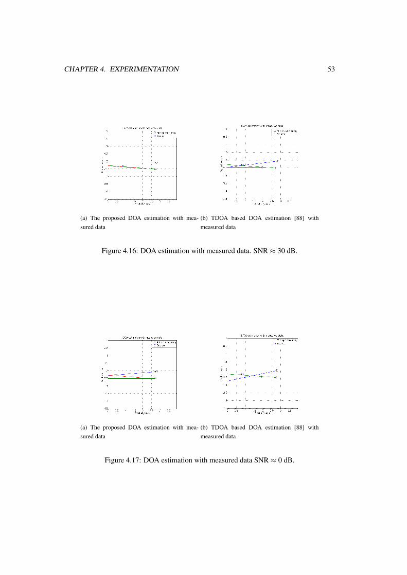
CHAPTER 4. EXPERIMENTATION 53
(a) The proposed DOA estimation with mea-sured data
(b) TDOA based DOA estimation [88] withmeasured data
Figure 4.16: DOA estimation with measured data. SNR ≈ 30 dB.
(a) The proposed DOA estimation with mea-sured data
(b) TDOA based DOA estimation [88] withmeasured data
Figure 4.17: DOA estimation with measured data SNR ≈ 0 dB.

CHAPTER 4. EXPERIMENTATION 54
for the PBF based DOA estimation method the microphone signals are downsampled to thePBF design sampling rate (8 kHz), the SNR of the signals used in TDOA estimation haveapproximately 7 dB better SNR than the signals used for the PBF based DOA method.
Figure 4.18 shows the DOA estimation when largest output power is used as the beamlevel estimate (Ws in Figure 4.18(a)) and when the largest SNR is used as the beam levelestimate (Wr in Figure 4.18(b)). Also, white noise is played from the loudspeaker 4 (asdefined in Figure 4.3) with sound pressure level of 72 dB measured 30 cm from the loud-speaker. Otherwise, the setting is the same as in the high SNR measurements in the previouschapters.
(a) DOA estimation with the largest outputpower.
(b) DOA estimation with the largest SNR.
Figure 4.18: DOA estimation. Measured data with white noise from loudspeaker 4.
Figure 4.18 shows similar behaviour as the simulated setup in Figure 4.13. The largestbeam power is still at the direction of the speaker and thus also DOA estimates are notsignificantly deviated from the correct DOA. Also as expected the direction with the highestSNR is not towards the speaker but it is deviated away from the noise source.
Multiple Arrays
As already mentioned when multiple microphone arrays are used, also the speaker loca-tion can be estimated. Here the speaker localization framework presented in this work isevaluated with measured data. The processing of the measured data is done by using thesame methods and parameters as the simulations in Chapter 4.4.2 in high and low SNR con-ditions. The speaker localization errors of the presented methods are shown in Table 4.3,where the loudspeaker number refers to the loudspeaker positions as defined in Figure 4.3.
As can be seen from the table, in reverberated conditions the proposed source localiza-tion method performs equally well also in low SNR. The table also shows the worst-case-

CHAPTER 4. EXPERIMENTATION 55
SNR SNR ≈ 30 dB SNR ≈ 0 dBMethod SLF LINE SLF LINE
Loudspeaker 1 0.298m 0.080m 0.246m 0.356m
Loudspeaker 2 0.224m 0.874m 0.231m 0.730m
Loudspeaker 3 0.252m 0.840m 0.222m 0.971m
Loudspeaker 4 0.451m 1.825m 0.406m 1.957m
Mean 0.306m 0.905m 0.276m 1.004m
STD 0.101m 0.715m 0.087m 0.684m
Table 4.3: Speaker localization error with measured data
performance of the minimum Euclidian distance method. When the source is at sourcelocation 2 although the DOA estimates do not deviate significantly from the real DOA(RMSE < 5), the DOA lines do not intersect at any point and therefore the source locationestimate falls to the boundaries of the room. This is also demonstrated in Figure 4.16(a),where the DOA estimates are plotted when the source is at location 2
When SLF method is used, the small differences in source location estimates can beexplained by the averaging of the region with the highest likelihood (equation 3.32). Thisregion changes its location, shape and size depending on the changes in SNR, reverberation,etc. and therefore the source localization can be more accurate in low SNR conditions thanin high SNR conditions (Loudspeaker 1, Loudspeaker 3 and Loudspeaker 4). However,more reliable system performance can be achieved by generating a large number of PBFbeams thus creating smaller regions with the highest likelihood.

Chapter 5
Conclusions and Future Work
In this work a Distributed Microphone Array System (DMAS) for a two-way audio com-munication application is presented. The goal of the proposed DMAS is to localize thedominant speech source and capture the speech signal with minimum degradations. Eachmicrophone array in the distributed system works as a Polynomial Beamformer [44] (PBF)and the output of the beamformers is used for the audio capture as well as for the speakerlocalization. The speaker localization is done by steering the PBF to several possible speechsource directions and estimating the signal power or Signal-to-Noise Ratio (SNR) of eachbeam. The speaker is estimated to be in the steering direction of the beam with highestpower or SNR. The fusing of the beam power data of each PBF is done by creating a SpatialLikelihood Function (SLF) by mapping the beam powers of each beam in each microphonearray to the acoustical environment and summing these beam powers together. Finally, thespeaker is localized to the point with highest value of SLF. The audio capture is done bysteering the PBF closest to the speech source to the direction of the localized speaker. Thisis done in order to maximize the Signal-to-Noise Ratio (SNR) of the PBF output signal.
The proposed two-way audio communication system as well as the DMAS was imple-mented to run in real-time on top of Pure Data signal processing environment. The im-plemented communication system uses 32 kHz sampling rate, thus enabling the transfer ofnearly full spectrum of human auditory system. To reduce the computational load of theadaptive acoustic echo cancelling algorithm, the adaptive echo cancelling is done only forthe low frequencies, while echo suppression techniques are used for higher frequencies.This enables an effective use of adaptive echo cancellation algorithms while at the sametime enabling good echo attenuation [80].
The performance of the proposed speaker localization framework was evaluated in simu-lated anechoic conditions and in real acoustic environment. It was found that the frameworkwas capable of locating the speaker in average error of 40 cm from the real speaker location.
56
CHAPTER 5. CONCLUSIONS AND FUTURE WORK 57
Also, it was shown that the PBF in the implemented microphone array achieves the max-imum attenuation of approximately 15 dB for the sounds arriving from the other than thePBF steering direction, thus reducing the effect of reverberation and noise in the capturedsignal. It was found out that the main restriction in the proposed framework is the finiteresolution of the sound source Direction Of Arrival (DOA) estimation. Due to this finiteresolution the SLF creates areas of highest values, which change size and shape when evensmall changes occur in the acoustical environment or in the sound source location. Thus,the proposed method can not be said to perform optimally in any circumstances.
However, the most important theoretical finding in this work is that in a distributed systemthe use of the beam with the best SNR to determine the speech source direction is not theobvious choice as compared to one array case. In general it can be said that in high SNRconditions using the beams with highest total power provides better results in a distributedsystem. This is because it was shown that in an environment with one dominant noisesource, the Direction Of Arrival (DOA) estimates are dependant of the noise source locationand not of the desired speech source location. This leads to larger errors when the deviateddata from each microphone array is combined.
Although the results show that the proposed speaker localization framework performswell under static conditions, the performance of the system with moving speakers shouldbe investigated. This might prove to be a challenging task because of the averaging ofthe power of each beam, which results in slowly reducing power in the beams adjacent tothe beam steered to the direction of the active speaker. Also, extensions to multiple activespeakers should be investigated.
To enable robust speaker localization in two-way audio communication setup an efficientVoice Activity Detector (VAD) should be implemented to the system. Without a VAD thespeaker location might change to the location of the loudspeakers that are used to renderthe far-end signal or also the speaker location might change even though there is no activespeaker. Also, when VAD is placed after the PBF, the VAD could be used to detect if severalspeakers are active at the same time at different spatial directions.
For the future work in the audio capture side, the formulation of PBF in the frequencydomain would enable better estimation of the noise power spectral densities of differentspatial directions and those could be used e.g. in spatial noise reduction. Also, Jia et al.describe a method combining the beams of each microphone array [41] and thus further in-creasing the system output SNR, but the benefits of multiple beamformers for audio captureshould be more thoroughly investigated.
However, the biggest obstacle in the efficient use of the proposed system in two-wayaudio communication setup is the constantly changing echo path due to the changes in thesteering direction and/or in the location of the microphone array that is used to capture the
CHAPTER 5. CONCLUSIONS AND FUTURE WORK 58
signal. When the echo path changes dramatically the echo cancellation algorithm has to usea large step size to adapt itself to the new echo path impulse response which results in audi-ble echo. Especially in multi-speaker conditions the beam steering direction might changerapidly, thus resulting an increasing echo. This problem can be decreased by placing anecho canceller after each microphone array instead of using just one echo canceller. How-ever, this in itself is not enough because not only the active microphone array is changingbut also the steering direction of each beamformer. To overcome this problem some kind ofecho path history could be used to improve the performance of the echo cancellation. Theidea is that every time a beamformer has a new steering direction, it checks if it has beensteered there before and retrieves the impulse response of the echo path that was used lasttime. This behavior would enable the echo canceller to start the adaptation from a closematch to the actual echo path impulse response, thus reducing the adaptation time.
However in the end the acceptance of new technologies comes down to the improvementsin the user experience of the system. Therefore, listening tests and user experience studiesshould be performed in order to find out how much beamforming with a distributed micro-phone array system improves telecommunication experience or if it is enough to have highquality audio hardware components to capture the audio signal.

Bibliography
[1] DPA miniature microphone specifications. http://www.dpamicrophones.
com/Images/DM01974.pdf. Last Checked: 16.7.2008.
[2] Genelec 1029a active monitor speaker. http://www.genelec.com/pdf/
DS1029a.pdf. Last Chacked: 28.8.2008.
[3] netsend∼/netrecieve∼ download page. http://www.nullmedium.de/dev/
netsend~/. Last Checked: 17.7.2008.
[4] Presonus Firepod user manual. http://www.presonus.com/media/
manuals/fpmanual.pdf. Last Checked: 16.7.2008.
[5] Parham Aarabi. The fusion of distributed microphone arrays for sound localization.EURASIP Journal of Applied Signal Processing (Special Issue on Sensor Networks),2003(4):338 – 347, 2003.
[6] Thibaut Ajdler, Igor Kozintsev, Rainer Lienhart, and Martin Vetterli. Acoustic sourcelocalization in distributed sensor networks. In Conference Record of the Thirty-EighthAsilomar Conference on Signals, Systems and Computers, pages 1328 – 1332, Novem-ber 2004.
[7] Ian F. Akyildiz, Weilian Su, Yogesh Sankarasubramaniam, and Erdal Cayirci. A sur-vey on sensor networks. IEEE Communications Magazine, 40(8):102 – 114, 2002.
[8] Jason Benesty and Dennis R. Morgan. Frequency-domain adaptive filtering revisited,generalization to the multi-channel case, and application to acoustic echo cancellation.In Int. Conf. on Acoustics, Speech and Signal Processing, pages 789 – 792, 2000.
[9] A.J. Berkhout, D. de Vries, and P. Vogel. Acoustic control by wave field synthesis.The Journal of the Acoustical Society of America, 93(5):2764 – 2778, 1993.
59

BIBLIOGRAPHY 60
[10] Stanley T. Birchfield and Rajitha Gangishetty. Acoustic localization by interaurallevel difference. In IEEE International Conference on Acoustics, Speech and SignalProcessing, pages 1109 – 1112, March 2005.
[11] Joerg Bitzer and K. Uwe Simmer. Superdirective microphone arrays. In MicahelBrandstein and Darren Ward, editors, Microphone Arrays: Signal Processing Tech-niques and Applications, pages 19 – 38. Springer, 2001.
[12] Radamis Botros, Onsy Abdel-Alim, and Peter Damaske. Stereophonic speech tele-conferencing. In IEEE International Conference on Acoustics, Speech and SignalProcessing, pages 1321 – 1324, April 1986.
[13] Michael Brandstein and Darren Ward. Microphone Arrays: Signal Processing Tech-niques and Applications. Springer, 2001.
[14] Herbert Buchner, Robert Aichner, and Walter Kellermann. A generalization of blindsource separation algorithms for convolutive mixtures based on second-order statis-tics. IEEE Transactions on Speech and Audio Processing, 13(1):120 – 134, January2005.
[15] Herbert Buchner, Wolfgang Herbordt, and Walter Kellermann. An efficient combi-nation of multi-channel acoustic echo cancellation with a beamforming microphonearray. In International Workshop on Hand-Free Speech Communication, pages 55–58, 2001.
[16] Herbert Buchner and Walter Kellermann. Acoustic echo cancellation for two andmore reproduction channels. In International Workshop on Acoustic Echo and NoiseControl, pages 99 – 102, 2001.
[17] G. Clifford Carter. Tutorial overview of coherence and time delay estimation. InCoherence and Time Delay Estimation, pages 1 – 27. IEEE Press, 1993.
[18] Y. T. Chan and K. C. Ho. A simple and efficient estimator for hyperbolic location.IEEE Transactions on Signal Processing, 42(8):1905 – 1915, 1994.
[19] Thomas Chou. Frequency-independent beamformer with low response error. In In-ternational Conference on Acoustics, Speech and Signal Processing, volume 5, pages2995 – 2998, Detroit, USA, 1995.
[20] Dirk Van Compernolle and Stefaan Van Gerven. Beamforming with micophone ar-rays. In V. Cappellini and A.R. Figueiras-Vidal, editors, COST 299: Applications ofDigital Signal Processing to Telecommunications, pages 107 – 131. E.U., 1995.

BIBLIOGRAPHY 61
[21] Joseph H. DiBiase, Harvey F. Silverman, and Michael S. Brandstein. Robust local-ization in reverberant rooms. In Micahel Brandstein and Darren Ward, editors, Mi-crophone Arrays: Signal Processing Techniques and Applications, pages 157 – 182.Springer, 2001.
[22] Simon Doclo and Marc Moonen. Gsvd-based optimal filtering for single and multimi-crophone speech enhancement. IEEE Transactions on Signal Processing, 50(9):2230– 2244, September 2002.
[23] Scott C. Douglas. Blind separation of acoustic signals. In Michael Brandstein andDarren Ward, editors, Microphone Arrays: Signal Processing Techniques and Appli-cations, pages 354 –380. Springer, 2001.
[24] Dan E. Dudgeon and Russell M. Mersereau. Multidimensional signal processing.Prentice Hall, 1983.
[25] Michael J. Evans, Anthony I. Tew, and James A. S. Angus. Spatial audio telecon-ferencing - which way is better? In The 4th International Conference on AuditoryDisplay, pages 29–38, 1997.
[26] Angelo Farina. Simultaneous measurement of impulse response and distortion with aswept-sine technique. In AES 108th Convention, Paris, France, February 2000.
[27] C.W. Farrow. A continuosly variable digital delay element. In IEEE InternationalSymposium on Circuits and Systems, pages 2641 – 2645, June 1988.
[28] J.L. Flanagan, D.A. Berkley, G.W. Elko, J.E. West, and M.M. Sondhi. Autodirectivemicrophone systems. Acustica, 73:58 – 71, 1991.
[29] J.L. Flanagan, J. D. Johnston, R. Zahn, and G.W. Elko. Computer-steered microphonearrays for sound transduction in large rooms. Journal of the Acoustical Society ofAmerica, 78(5):1508 – 1518, 1985.
[30] Andre Gilloire. Experiments with sub-band acoustic echo cancellers for teleconfer-encing. In IEEE International Conference on Acoustics, Speech and Signal Process-ing, volume 12, pages 2141 – 2144, April 1987.
[31] Lloyd J. Griffiths and Charlse W. Jim. An alternative approach to linearly constrainedadaptive beamforming. IEEE Transactions on Antennas and Propagation, 30(1):27 –34, 1982.
BIBLIOGRAPHY 62
[32] Timo Haapsaari, Werner de Brujin, and Aki Härmä. Comparison of different soundcapture and reproduction techniques in a virtual acoustic window. In AES 122ndConvention, Vienna, Austria, May 2007.
[33] Simon Haykin. Array Signal Processing. Prentice-Hall, 1984.
[34] Wolfgang Herbordt, Herbert Buchner, Walter Kellermann, Rudolf Rabenstein, SaschaSpors, and H. Teutsch. Full-duplex multichannel communication: real-time imple-mentations in a general framework. In International Conference on Multimedia andExpo, pages 49 – 52, 2003.
[35] Wolfgang Herbordt, Herbert Buchner, Satoshi Nakamura, and Walter Kellermann.Multichannel bin-wise robust frequency-domain adaptive filtering and its applicationto adaptive beamforming. IEEE Transactions on Audio, Speech and Language Pro-cessing, 15(4):1340 – 1351, 2007.
[36] Wolfgang Herbordt and Walter Kellermann. Adaptive beamforming for audio signalacquisition. In Adaptive Signal Processing - Applications to Real-World Problems,pages 155 – 194. Springer, 2003.
[37] Osamu Hoshuyama and Akihiko Sugiyama. Robust adaptive beamforming. InMichael Brandstein and Darren Ward, editors, Microphone Arrays: Signal ProcessingTechniques and Applications, pages 87 – 109. Springer, 2001.
[38] Yiteng Huang, Jacob Benesty, Gary W. Elko, and Russell M. Mersereau. Rea-timepassive source localization: A practical linear-correction leas squares approach. IEEETransactions on Speech and Audio Processing, 9(8):943 – 956, 2001.
[39] Jyri Huopaniemi. Virtual Acoustics and 3-D Sound in Multimedia Signal Processing.PhD thesis, Helsinki University of Technology, Department of Electrical and Com-munications Engineering, 1999.
[40] Matti Hämäläinen and Ville Myllylä. Acoustic echo cancelation for dynamicallysteered microphone array systems. In Proc. of the IEEE Workshop of Applicationsof Signal Processing to Audio and Acoustics, New Paltz, NY, October 2007.
[41] Ying Jia, Yu Luo, Yan Lin, and Igor Kozintsev. Distributed microphone arrays fordigital home and office. In IEEE International Conference on Acoustics, Speech andSignal Processing, volume 5, May 2006.
[42] Don H. Johnson and Dan E. Dudgeon. Array Signal Processing. Prentice Hall, 1993.

BIBLIOGRAPHY 63
[43] Matti Kajala and Matti Hämäläinen. Broadband beamforming optimization for speechenhancement in noisy environments. In IEEE Worshop on Applications of SignalProcessing to Audio and Acoustics, pages 19 – 22, 1999.
[44] Matti Kajala and Matti Hämäläinen. Filter-and-sum beamformer with adjustable filtercharacteristics. In IEEE International Conference on Acoustics and Speech and SignalProcessing, volume 5, pages 2917 – 2920, Salt Lake City, USA, May 2001.
[45] Walter Kellermann. A self-steering digital microphone array. In IEEE InternationalConference on Acoustics, Speech and Signal Processing, volume 5, pages 3581 –3584, Toronto, Canada, April 1991.
[46] Walter Kellermann. Acoustic echo cancellation for beamforming microphone arrays.In Michael Brandstein and Darren Ward, editors, Microphone Arrays: Signal Process-ing Techniques and Applications, pages 281 – 306. Springer, 2001.
[47] Zhiyun Li and Ramani Duraiswami. Hemispherical microphone arrays for sound cap-ture and beamforming. In IEEE Workshop on Applications of Signal Processing toAudio and Acoustics, pages 106 – 109, October 2005.
[48] Hui Liu and Evangelos Milios. Acoustic positioning using multiple microphone ar-rays. The Journal of the Acoustical Society of America (JASA), 117(5):2772 – 2782,May 2005.
[49] David G. Malham and Anthony Myatt. 3-d sound spatialization using ambisonic tech-niques. Computer Music Journal, 19(4):58 – 70, 1995.
[50] Rainer Martin. An efficient algorithm to estimate the instantaneous snr of speech sig-nals. In Proceedings of European Conference on Speech Communication and Tech-nology (EUROSPEECH), pages 1093 – 1096, Berlin, Germany, September 1993.
[51] Rainer Martin. Noise power spectral density estimation based on optimal smoothingand minimum statistics. IEEE Transactions on Speech and Audio Processing, 9(5):504– 512, 2001.
[52] Mar Marzinzik and Birger Kollmeier. Speech pause detection for noise spectrumestimation by tracking power envelope dynamics. IEEE Transactions on Speech andaudio Processing, 10:109 – 118, 2002.
[53] Robert C. Michael Williamson. Multichannel sound recording practice using micro-phone arrays. In 24th International Conference: Multichannel Audio, The New Real-ity, 2003.
BIBLIOGRAPHY 64
[54] Henrik Møller. Fundamentals of binaural technology. Applied Acoustics, 36(3-4):171–218, 1991.
[55] Ville Myllylä. Residual echo filter for enhanced acoustic echo control. Signal Pro-cessing, 86(6):1193–1205, 2006.
[56] Ville Myllylä and Matti Hämäläinen. Adaptive beamforming methods for dynami-cally steered microphone array systems. In IEEE International Conference Acoustics,Speech and Signal Processing, Las Vegas, USA., Mar. 2008.
[57] Michael Syskind Pedersen, Jan Larsen, Ulrik Kjems, and Lucas C. Parra. A surveyof convolutive blind source separation methods. In Springer Handbook of SpeechProcessing. Springer, November 2007.
[58] Jonathan Postel. User datagram protocol. RFC 768, USC/Information Sciences Insti-tute, August 1980.
[59] Jonathan Postel. Transmission control protocol. RFC 793, USC/Information SciencesInstitute, September 1981.
[60] Ilyas Potamitis, Huimin Chen, and George Tremoulis. Tracking of multiple movingspeakers with multiple microphone arrays. IEEE Transations on Speech and AudioProcessing, 12(5):520 – 529, September 2004.
[61] Miller Puckette. Pure Data: Another integrated computer music environment. InSecond Intercollege Computer Music Concerts, pages 37–41, Tachikawa, Japan, 1996.
[62] Miller Puckette. Max at seventeen. Computer Music Journal, 26(4):31–43, 2002.
[63] Ville Pulkki. Virtual sound source positioning using vector base amplitude panning.Journal of the Audio Engineering Society (JAES), 45(6):456–466, June 1997.
[64] Ville Pulkki. Spatial Sound Generation and Perception by Amplitude Panning Tech-niques. PhD thesis, Helsinki University of Technology, Department of Electrical andCommunications Engineering, 2001.
[65] Boaz Rafaely. Analysis and design of spherical microphone arrays. IEEE Transactionson Speech and Audio Processing, 13(1):135 – 143, 2005.
[66] Mika Ristimäki, Matti Hämäläinen, Julia Turku, and Riitta Väänänen. A cross-platform audio signal processing environment for real-time audio algorithm devel-opment. In AES 124th Convention, Amsterdam, The Netherlands, May 2008.
BIBLIOGRAPHY 65
[67] Gabrielle H. Saunders and James M. Kates. Speech intelligibility enhancement us-ing hearing-aid array processing. Journal of the Acoustical Society of America,102(3):1827 – 1837, September 1997.
[68] H. Sculzrinne, S. Casner, R. Frederick, and V. Jacobson. RTP: A transport protocolfor real-time applications. RFC 3550, USC/Information Sciences Institute, July 2003.
[69] Xiaohong Sheng and Yu-Hen Hu. Maximum likelihood multiple-source localizationusing acoustic energy measurements with wireless sensor networks. IEEE Transac-tions on Signal Processing, 53(1):44 – 53, 2005.
[70] Harvey F. Silverman. Some analysis of microphone arrays for speech data acquisition.IEEE Transactions on Acoustics, Speech and Signal Processing, 35(12):1699 – 1712,1987.
[71] Harvey F. Silverman, William R. Patterson, and James L. Flanagan. The huge micro-phone array. IEEE Concurrency, 6(4):36 – 46, 1998.
[72] K. Uwe Simmer, Joerg Bitzer, and Claude Marro. Post-filtering techniques. In MichaelBrandstein and Darren Ward, editors, Microphone Arrays: Signal Processing Tech-niques and Applications, pages 39 – 57. Springer, 2001.
[73] M. Mohan Sondhi, Dennis R. Morgan, and Jospeh L. Hall. Stereophonic acousticecho cancellation – An overview of the fundamental problem. IEEE Signal ProcessingLetters, 2(8):148 – 151, 1995.
[74] Sascha Spors, Rudolf Rabenstein, and Jens Ahrens. The theory of wave field syntesisrevisited. In AES 124th Convention, Amsterdam, The Netherlands, May 2008.
[75] Harry L. Van Trees. Optimium Array Processing. John Wiley & Sons, 2002.
[76] P. P. Vaidyanathan. Multirate digital filters, filter banks, polyphase networks, andapplications: a tutorial. Proceedings of the IEEE, 78(1):56 – 93, 1990.
[77] Päivi Valve. Method and system for tracking human speakers. US Patent 6449593,2001.
[78] Menno van der Wal, Evert W. Start, and Diemer Vries. Design of logarithmicallyspaced constant-directivity transducer arrays. Journal of the Audio Engineering Soci-ety, 44(6):497 – 507, 1996.
[79] Barry D. Van Veen and Kevin M. Buckley. Beamforming: Averstile approach tospatial filtering. IEEE ASSP Magazine, 5(2):4 – 24, 1988.
BIBLIOGRAPHY 66
[80] Frederik Wallin and Chrisof Faller. Perceptual quality of hybrid echo can-celler/suppressor. In IEEE International Conference Acoustics, Speech and SignalProcessing, volume 4, pages 157–160, May 2004.
[81] Darren B. Ward, Rodney A. Kennedy, and Robert C. Williamson. Theory and designof braodband sensor arrays with frequency invariant far-field beam patterns. Journalof the Acoustical Society of America, 97:1023 – 1034, 1995.
[82] Darren B. Ward, Rodney A. Kennedy, and Robert C. Williamson. Fir filter designfor frequency invariant beamfromers. IEEE Signal Processing Letters, 3(3):69 – 71,1996.
[83] Darren B. Ward, Rodney A. Kennedy, and Robert C. Williamson. Constant direc-tivity beamforming. In Michale Brandstein and Darren Ward, editors, MicrophoneArrays:Signal Processing Techniques and Applications, pages 3 – 18. Springer, 2001.
[84] Darren B. Ward, Eric A. Lehmann, and Robert C. Williamson. Particle filtering algo-rithms for tracking an acoustic source in a reverberant environment. IEEE Transac-tions on Speech and Audio Processing, 11(6):826 – 836, 2003.
[85] Eugene Weinstein, Kenneth Sttele, Anant Agarwak, and James Glass. Loud: A 1020-node microphone array and acoustic beamformer. In International Congress on soundand Vibration (ICSV), Cairns, Australia, July 2007.
[86] J.E. West, J. Blauert, and D.J. MacLean. Teleconferencing system using head-relatedsignals. Applied Acoustics, 36(3-4):327 – 333, 1991.
[87] Takeshi Yamada, Satoshi Nakamura, and Kiyohiro Shikano. Distant-talking speechrecognition based on a 3-d viterbi search using a microphone array. IEEE Transactionson Speech and Audio Processing, 10(2):48 – 56, February 2002.
[88] Jari Yli-Hietanen, Kari Kalliojärvi, and Jaakko Astola. Low-complexity angle of ar-rival estimation of wideband signalsusing small arrays. In 8th IEEE Signal ProcessingWorkshop on Statistical Signal and Array Processing, pages 109 – 112, 1996.