distributed matrix product state simulations of large
TRANSCRIPT
Distributed Matrix Product State Simulationsof Large-Scale Quantum Circuits
Aidan Dang
A thesis presented for the degree of
Master of Scienceunder the supervision of
Dr. Charles Hill and Prof. Lloyd Hollenberg
School of PhysicsThe University of Melbourne
20 October 2017
Abstract
Before large-scale, robust quantum computers are developed, it is valuable to be able to clas-sically simulate quantum algorithms to study their properties. To do so, we developed a nu-merical library for simulating quantum circuits via the matrix product state formalism ondistributed memory architectures. By examining the multipartite entanglement present acrossShor’s algorithm, we were able to effectively map a high-level circuit of Shor’s algorithm to theone-dimensional structure of a matrix product state, enabling us to perform a simulation of aspecific 60 qubit instance in approximately 14 TB of memory: potentially the largest non-trivialquantum circuit simulation ever performed. We then applied matrix product state and ma-trix product density operator techniques to simulating one-dimensional circuits from Google’squantum supremacy problem with errors and found it mostly resistant to our methods.
1
Declaration
I declare the following as original work:
• In chapter 2, the theoretical background described up to but not including section 2.5had been established in the referenced texts prior to this thesis. The main contributionto the review in these sections is to provide consistency amongst competing conventionsand document the capabilities of the numerical library we developed in this thesis. Therest of chapter 2 is original unless otherwise noted.
• The techniques and experimental results of chapters 3 and 4 are original unless otherwisestated.
I declare that the code for our numerical library was written solely by the author, where anyexternal libraries called have otherwise been referenced in this text.
Aidan DangOctober 2017
Acknowledgements
Most importantly, I give my gratitude to Doctor Charles Hill and Professor Lloyd Hollenberg fortheir guidance and vision in directing this work, for providing me with the resources necessaryto produce the results of this thesis and for pushing me to realise my potential.
In aiding the development of our numerical library and the production of our results, Iacknowledge that this work was supported by resources provided by the Pawsey Supercom-puting Centre with funding from the Australian Government and the Government of WesternAustralia.
To The University of Melbourne, and especially the School of Physics, I am thankful to havebeen in an environment that would fuel the growth of my abilities. In order that I may focuson my studies, I would also like to thank Ms Rose Cooney, Ms Jenny de Boer and AssociateProfessor Michelle Livett for greatly simplifying the daunting administrative matters that I wasfaced with.
Finally, to all the friends, classmates, teachers and students that I have ever had, and anyoneelse I have ever learned something from, I hope that you might have gained something fromme in return.
2
Contents
1 Introduction 4
2 QCMPS Library Showcase 82.1 Introduction to tensor networks . . . . . . . . . . . . . . . . . . . . . . . . . . . 8
2.1.1 Reshape and transpose . . . . . . . . . . . . . . . . . . . . . . . . . . . . 92.1.2 Contraction and tensor product . . . . . . . . . . . . . . . . . . . . . . . 92.1.3 Decomposition . . . . . . . . . . . . . . . . . . . . . . . . . . . . . . . . 10
2.2 Quantum circuits as tensor networks . . . . . . . . . . . . . . . . . . . . . . . . 102.3 Matrix Product States . . . . . . . . . . . . . . . . . . . . . . . . . . . . . . . . 132.4 QCMPS . . . . . . . . . . . . . . . . . . . . . . . . . . . . . . . . . . . . . . . . 13
2.4.1 MPS canonical form . . . . . . . . . . . . . . . . . . . . . . . . . . . . . 142.4.2 Contraction and decomposition . . . . . . . . . . . . . . . . . . . . . . . 152.4.3 Recanonicalisation and renormalisation . . . . . . . . . . . . . . . . . . . 162.4.4 Truncation . . . . . . . . . . . . . . . . . . . . . . . . . . . . . . . . . . . 172.4.5 Measurement and reset . . . . . . . . . . . . . . . . . . . . . . . . . . . . 182.4.6 Gate operations . . . . . . . . . . . . . . . . . . . . . . . . . . . . . . . . 19
2.5 General controlled gate operations for MPS . . . . . . . . . . . . . . . . . . . . 212.6 Density matrices in MPS . . . . . . . . . . . . . . . . . . . . . . . . . . . . . . . 24
2.6.1 Error model simulations with MPDOs . . . . . . . . . . . . . . . . . . . 262.6.2 Alternate approaches for density matrix simulations . . . . . . . . . . . . 27
2.7 Comparison to existing quantum simulators . . . . . . . . . . . . . . . . . . . . 28
3 Shor’s Algorithm Simulations 293.1 Review of Shor’s algorithm . . . . . . . . . . . . . . . . . . . . . . . . . . . . . . 293.2 Entanglement in Shor’s algorithm . . . . . . . . . . . . . . . . . . . . . . . . . . 313.3 MPS simulation approach . . . . . . . . . . . . . . . . . . . . . . . . . . . . . . 32
3.3.1 Previous approaches . . . . . . . . . . . . . . . . . . . . . . . . . . . . . 323.3.2 Simulation through QCMPS . . . . . . . . . . . . . . . . . . . . . . . . . 33
3.4 Benchmarks . . . . . . . . . . . . . . . . . . . . . . . . . . . . . . . . . . . . . . 343.5 Future simulations . . . . . . . . . . . . . . . . . . . . . . . . . . . . . . . . . . 36
4 Google Supremacy Circuit Simulations 374.1 Introduction to the Google supremacy problem . . . . . . . . . . . . . . . . . . 374.2 One-Dimensional Circuit . . . . . . . . . . . . . . . . . . . . . . . . . . . . . . . 40
4.2.1 Porter-Thomas Convergence . . . . . . . . . . . . . . . . . . . . . . . . . 404.3 MPS Truncation . . . . . . . . . . . . . . . . . . . . . . . . . . . . . . . . . . . 404.4 MPDO Noise Channel Simulations . . . . . . . . . . . . . . . . . . . . . . . . . 42
5 Conclusion 45
3
Chapter 1
Introduction
Despite the vast progress made in order to realise modern computing devices from a mathe-matical model, the Turing machine [1], this underlying model imposes limitations on the typesof problems that such a ‘classical’ computer may solve, and the efficiency with which it mightdo so. Although the time required to solve a computable problem on a classical machine doesdecrease if we use more or faster hardware, there exist particularly consequential problems that,given a sufficiently large instance, may not be solved with any reasonable amount of time orhardware using our best known classical algorithms.
This presents several paths forward. Lacking proof that our current classical algorithmsfor these problems obtain solutions with optimal efficiency, one approach might be to developmore efficient algorithms for our existing devices, an active area of research in computer sciencetoday. Another is to subscribe to a different model of computation, in which algorithms existfor solving these problems efficiently. Indeed, with a quantum computer based on the quantumcircuit model of computation, solutions for problems such as integer factorisation [2] may beobtained efficiently.
The concept of these quantum machines that potentially possess some inherent speed advan-tage over their classical counterparts motivates their physical construction, with the experimen-tation and engineering required in their implementation needing to stave off the effects of noiseand decoherence in order to scale. Before such large-scale quantum computers can be built,methods to simulate their specific behaviours and interactions with quantum circuits shouldstill prove valuable. Though the ability to perform such simulations would still be subject tothe limitations of classical computation, it may, for example, allow us to study a quantumcircuit’s resilience toward these noise effects on specific proposed hardware implementations.
Despite this quantum advantage over currently known classical algorithms for these prob-lems, the presence of an innate advantage is still uncertain. However, in order to high-light perceived speed differences between the quantum and classical models, several ‘quantumsupremacy’ problems have been proposed, with the aim of being efficiently solvable on quan-tum hardware but not efficiently solvable classically. Often, these problems claim a ‘supremacypoint’, a sufficiently large instance size that a reasonable amount of classical hardware may notsolve in a reasonable amount of time; a quantum device that successfully solves problems of thissize are then said to demonstrate quantum supremacy. Currently, physical implementations ofquantum computers are unable to claim quantum supremacy.
Quantum computation and algorithms
If the states that comprise a quantum mechanical system form a d-dimensional Hilbert spaceH, then n such systems form the dn-dimensional Hilbert space H⊗n. If we consider a system of2-dimensional subsystems, then the values 0 and 1 can be assigned to these levels to produce a
4
quantum bit or qubit, the quantum counterpart to the bit in classical computation. Since a stateof this composite system resides as an element within H⊗n, familiar quantum properties suchas superposition and entanglement are applicable. For example, a collection of n bits allows usto store exactly one value out of the 2n possible binarily representable values, whilst a set of nquantum bits may describe a superposition of all these 2n values. It would then appear thatany speed advantage of a quantum computer arises from these exclusively quantum properties.However, the extent to which each of these properties contributes to the perceived advantageis not fully understood [3].
Just as classical bits are manipulated as electrical signals passing through circuits of logicgates in a classical computer, the quantum circuit model of computation involves acting quan-tum gates on one or more of the quantum system’s constituent subsystems. In quantum me-chanical terms, these gates act as unitary transformations on the quantum state. Therefore,unlike most classical logic gates, applying a quantum gate is a reversible operation, which hasconsequences on the information entropy content of a state [4]. Furthermore, measurement ofa quantum state to extract information from it, such as the results of a quantum algorithm,necessarily alters the state via a collapse of superposition and entanglement, unlike in a systemof classical bits. Quantum algorithmic design must therefore keep these constraints in mind.
It is also worth mentioning that other quantum models of computation exist. Notably, thequantum Turing machine as a generalisation of the classical Turing machine is considered com-putationally equivalent to the quantum circuit model [5], and implementations based on thesemodels are referred to as universal quantum computers. Additionally, an adiabatic quantumcomputer [6] functions by initialising a system to the ground state of a simple Hamiltonian andadiabatically evolving it so that the system remains in the ground state, but of a Hamiltonianwhere this ground state encodes the solution to the relevant problem.
The efficiency of any computational algorithm often refers to its time complexity: thescaling of the algorithm’s running time with respect to its input size. Specifically, we express analgorithm’s time complexity in terms of its time usage’s asymptotic behaviour using Bachmann–Landau notation. To demonstrate, classical lookup of a single item from a black-box databaseof N items has an average time complexity of O(N), as each item must be sequentially querieduntil the relevant entry is found. However, Grover’s algorithm [7], performed on a quantumcomputer, allows this task to be performed in O(
√N) time, resulting in a quadratic advantage
over the classical approach. When a symmetric-key cryptographic algorithm such as AES [8]with a key of length n bits is used in place of this black-box database, the O(N = 2n) lookupsfor the classical approach is reduced to O(
√N = 2n/2) operations through Grover’s algorithm,
and therefore halving the effective key length.An algorithm is said to be efficient if its time complexity is bounded above by some poly-
nomial. With this definition, Grover’s algorithm is not sufficient to efficiently break AESencryption by searching through all possible keys. Factorisation of an integer of length n dig-its is one example of a problem that can be solved in polynomial time with respect to n ona quantum computer through Shor’s algorithm [2], but lacks any known algorithm to do soefficiently on a classical machine. Therefore, quantum computers currently exhibit an exponen-tial speed advantage over classical computers in integer factorisation. Many of the public-keycryptographic protocols [9] presently used for online communications are predicated on the dif-ficulty of integer factorisation and the discrete logarithm problem (which Shor’s algorithm alsosolves efficiently), so post-quantum cryptographic protocols resistant to attacks by quantumcomputers have been proposed [10] in response.
5
Supremacy problems
Given the multitude of quantum algorithms that provide a computational speedup over theirfastest known classical counterparts [11], it is still an open question in computer science as towhether or not these quantum computers, based on the various quantum models of computationsuch as the circuit model, innately possess some computational advantage over our classicaldevices built upon the Turing machine. The difficulty in proving the existence of this advantage,i.e. the existence of quantum supremacy, stems from bounding the computational power ofclassical machines; though some classical algorithms are bested by quantum algorithms interms of their time complexity, these quantum algorithms must demonstrate their advantageover all possible classical algorithms in order to prove quantum supremacy, and not just overthe classical algorithms that are known.
Even if quantum supremacy were theoretically possible, there still remains the experimentalchallenges in building a physical machine to demonstrate it. As a physical quantum deviceinteracts with its environment over the course of a circuit, effects such as quantum decoherenceand noise begin to alter its internal quantum state in ways extraneous to the circuit’s gates,potentially leading to errors in any results obtained through measurement. Quantum errorcorrection codes such as the surface code [12] have been developed to increase the resilienceof physical quantum computers toward noise and decoherence, at the cost of requiring greaterredundancy in the number of qubits.
Despite the theoretical and experimental challenges in demonstrating quantum supremacy,problems designed to be efficiently solvable through a quantum model of computation butnot through any known classical algorithm have been proposed as tests [13]. Often, these aresampling problems: a quantum device will perform some efficient manipulation of a quantumstate and sample measurements from the resulting underlying probability distribution. It isthen argued that classical computers cannot efficiently reproduce this probability distributionto sample from, given some specification of the quantum operation involved (e.g. the quantumcircuit). In the case of boson sampling [14], the device is a linear optical quantum computerthat manipulates Fock states of input photons via a linear optical network. Given the bestknown classical algorithms for simulating the results of these networks [14], it is estimatedthat instances of boson sampling with 50 photons exceed the capabilities of modern classicalhardware [15].
In the quantum circuit model, IQP (instantaneous quantum polynomial-time) [16] circuitsand the circuits proposed by Google’s Boixo et al. [17] involve sampling from the measurementresults of circuits randomly generated according to a set of rules. In both examples, noiseprevents a physical quantum computer from exactly sampling from the ideal distribution. In[17], a measure of how well a noisy quantum computer may sample from the ideal distributionproduced from one of their circuits is related to the effective per-gate error rate of the physicalimplementation. This allows a physical quantum computer’s effectiveness at Google’s samplingproblem to be compared to a classical simulation’s, despite being subject to the effects of noiseand errors.
Simulation techniques
For a two-level quantum system of Hilbert space H with basis elements labelled {|0〉 , |1〉} usedto represent a qubit, the evolution of a quantum system of n qubits in state |ψ〉 through theunitary transformations of a quantum gate takes place within the 2n-dimensional Hilbert spaceH⊗n, whose basis elements are
{|0 . . . 0〉 , |0 . . . 1〉 , . . . , |1 . . . 1〉} ≡ {|0〉 ⊗ . . .⊗ |0〉 , |0〉 ⊗ . . .⊗ |1〉 , . . . , |1〉 ⊗ . . .⊗ |1〉}.
6
Computationally, |ψ〉 can be described as a vector storing its 2n complex coefficients in this basisfor its Hilbert space H⊗n, and linear operators such as the unitary gate transformations maybe applied via matrix multiplication with its matrix representation in the same basis. Softwarepackages [18, 19] that perform simulations of the evolution of quantum states in this mannerare accordingly referred to as state vector simulators. Despite any properties of the quantumstate that might change over the course of, say, a quantum circuit, the state vector formalismimposes a strictO(2n) space complexity to simply store this state vector. For example, the 2 PiBrequired to store an n = 48 qubit state vector with 64 bit per complex coefficient approaches thelimit of memory available to modern supercomputers [15]. Furthermore, simulating quantumstate evolution via matrix multiplication on these state vectors has an exponentially scalingtime cost. Therefore, state vector simulations cannot currently be performed efficiently onclassical hardware.
An alternative representation of a quantum state |ψ〉 might instead adaptively scale itstime and space requirements according to some physical property of the state. Based onthe idea of tensor networks [20], Vidal [21] proposed the idea of using matrix product states(MPSs) as a representation of quantum states for simulating quantum circuits. The MPSformalism was originally used for other applications in condensed matter physics, namely fordetermining ground states of quantum systems through the density matrix renormalisationgroup (DMRG) algorithm [22] and simulating the time evolution of quantum states through agiven Hamiltonian [23]. In the MPS representation of a quantum state, if subsystems are laidout in a one-dimensional lattice, then only information about a subsystem and its entanglementwith the adjacent subsystems needs to be stored. Therefore, the space and time requirementsto store and operate on an MPS may scale with the amount of entanglement present in therepresented quantum state, where the ‘amount’ of entanglement is quantified by a particularmeasure. For Hamiltonians, quantum circuits or other quantum operators that do not introducelarge amounts of entanglement, the MPS representation may be used to efficiently simulate [23]these quantum systems on classical hardware.
Though the state vector and matrix product state formalisms are suited for simulation ofpure quantum states, modelling errors in a simulation of physical quantum hardware invitesconsideration of the density operator ρ =
∑i |ψi〉〈ψi| for mixed states. The density matrix for-
malism for representing the density operator of a d-dimensional state involves storing a matrixof dimension d×d, and is the mixed state counterpart for the state vector formalism. Similarly,the matrix product state formalism may be generalised to a matrix product density operatorformalism that also scales its time and space requirements for the amount of entanglement.
Outline
This thesis is focused on the development and features of our distributed-memory matrix prod-uct state software library, QCMPS, as well as a demonstration of its capabilities by simulatingShor’s algorithm and the Google supremacy problem. Chapter 2 provides a more formal intro-duction to the tensor network formalism that underpins the mechanics of MPSs, and introducesthe functionality of QCMPS with a comparison to existing quantum simulators. In chapter 3,we benchmark QCMPS with a high-level simulation of Shor’s algorithm following the method of[24] with additional optimisations to better suit the computation to MPSs. Using approximately14 TB of memory on the Magnus supercomputer [25], we were able to simulate an instance ofShor’s algorithm on 60 qubits, being potentially the largest high-level but non-trivial quantumcircuit ever simulated. Finally, we investigate the one-dimensional Google supremacy problemwith and without errors to determine if any of our MPS techniques might serve to refine theestimate for its supremacy point.
7
Chapter 2
QCMPS Library Showcase
The matrix product state formalism is a method for representing quantum states alternativeto the more familiar state vector formalism. As we discuss in this chapter, the time andspace requirements for storing and manipulating these matrix product states (MPSs) scalewith the amount of entanglement within the quantum state, making it a viable alternative foruse in classical simulations of certain quantum systems [21] when compared to the state vectorformalism with its more rigid requirements.
Since the use of MPSs for classical simulation of quantum circuits forms the basis of thisthesis, we will provide an introduction to their mechanics and an overview of the operationsthat can be performed with them. To begin, we introduce the use of tensor networks [20] forits convenient pictorial representations of the methods performed. The mechanics of MPSs canthen be built on this foundation.
To implement these operations, we have developed the numerical library QCMPS for sim-ulating quantum circuits. It is specifically tailored for this purpose, as opposed to simulatingother systems relevant to condensed matter physics [22, 23], so we document our choice ofconventions and our design decisions here.
2.1 Introduction to tensor networks
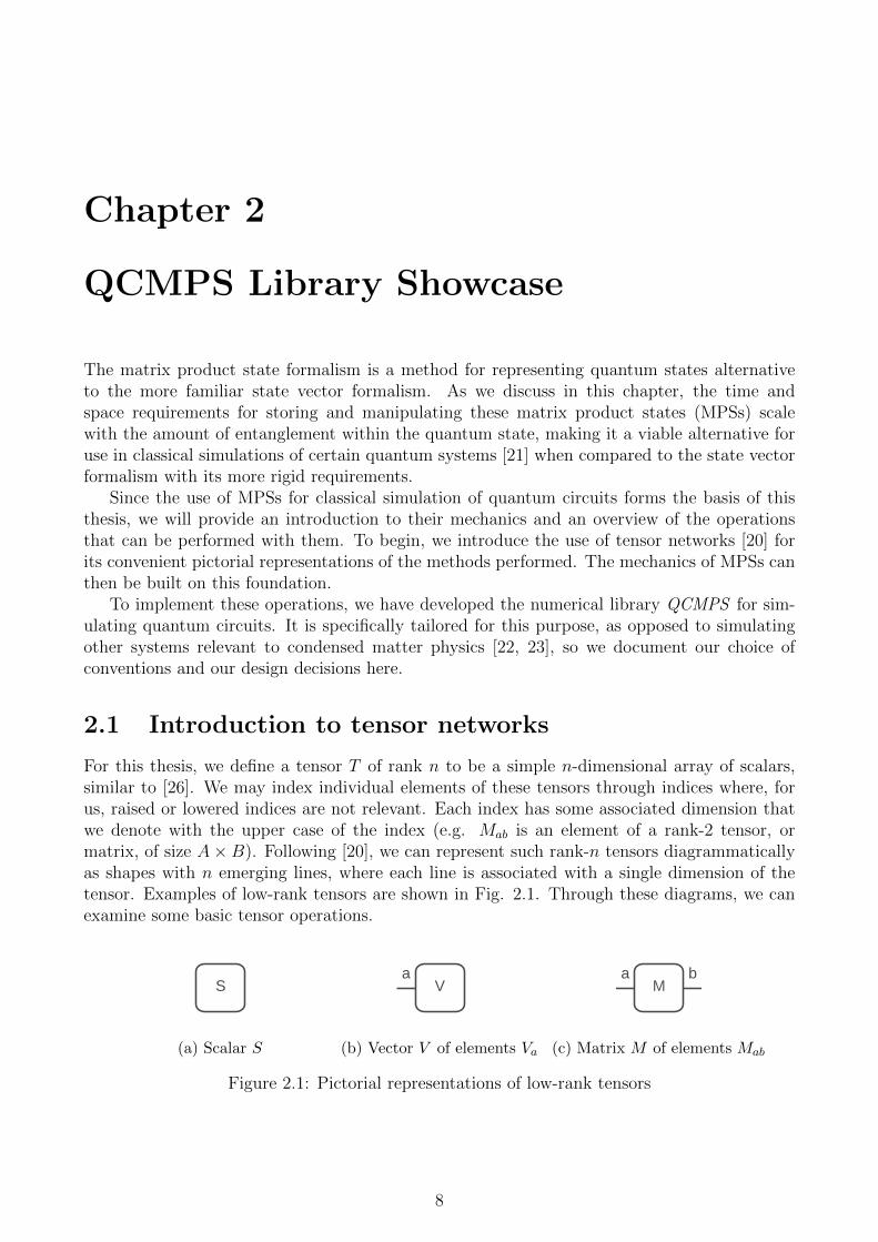
For this thesis, we define a tensor T of rank n to be a simple n-dimensional array of scalars,similar to [26]. We may index individual elements of these tensors through indices where, forus, raised or lowered indices are not relevant. Each index has some associated dimension thatwe denote with the upper case of the index (e.g. Mab is an element of a rank-2 tensor, ormatrix, of size A×B). Following [20], we can represent such rank-n tensors diagrammaticallyas shapes with n emerging lines, where each line is associated with a single dimension of thetensor. Examples of low-rank tensors are shown in Fig. 2.1. Through these diagrams, we canexamine some basic tensor operations.
S
(a) Scalar S
Va
(b) Vector V of elements Va
Ma b
(c) Matrix M of elements Mab
Figure 2.1: Pictorial representations of low-rank tensors
8
2.1. INTRODUCTION TO TENSOR NETWORKS
2.1.1 Reshape and transpose
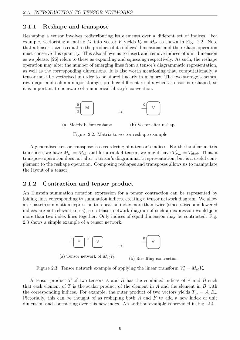
Reshaping a tensor involves redistributing its elements over a different set of indices. Forexample, vectorising a matrix M into vector V yields Vc = Mab as shown in Fig. 2.2. Notethat a tensor’s size is equal to the product of its indices’ dimensions, and the reshape operationmust conserve this quantity. This also allows us to insert and remove indices of unit dimensionas we please: [26] refers to these as expanding and squeezing respectively. As such, the reshapeoperation may alter the number of emerging lines from a tensor’s diagrammatic representation,as well as the corresponding dimensions. It is also worth mentioning that, computationally, atensor must be vectorised in order to be stored linearly in memory. The two storage schemes,row-major and column-major storage, produce different results when a tensor is reshaped, soit is important to be aware of a numerical library’s convention.
Ma
b
(a) Matrix before reshape
→V
c
(b) Vector after reshape
Figure 2.2: Matrix to vector reshape example
A generalised tensor transpose is a reordering of a tensor’s indices. For the familiar matrixtranspose, we have M>
ba = Mab, and for a rank-4 tensor, we might have T ′dbac = Tabcd. Thus, atranspose operation does not alter a tensor’s diagrammatic representation, but is a useful com-plement to the reshape operation. Composing reshapes and transposes allows us to manipulatethe layout of a tensor.
2.1.2 Contraction and tensor product
An Einstein summation notation expression for a tensor contraction can be represented byjoining lines corresponding to summation indices, creating a tensor network diagram. We allowan Einstein summation expression to repeat an index more than twice (since raised and loweredindices are not relevant to us), so a tensor network diagram of such an expression would joinmore than two index lines together. Only indices of equal dimension may be contracted. Fig.2.3 shows a simple example of a tensor network.
Ma b
V
(a) Tensor network of MabVb
→V'
a
(b) Resulting contraction
Figure 2.3: Tensor network example of applying the linear transform V ′a = MabVb
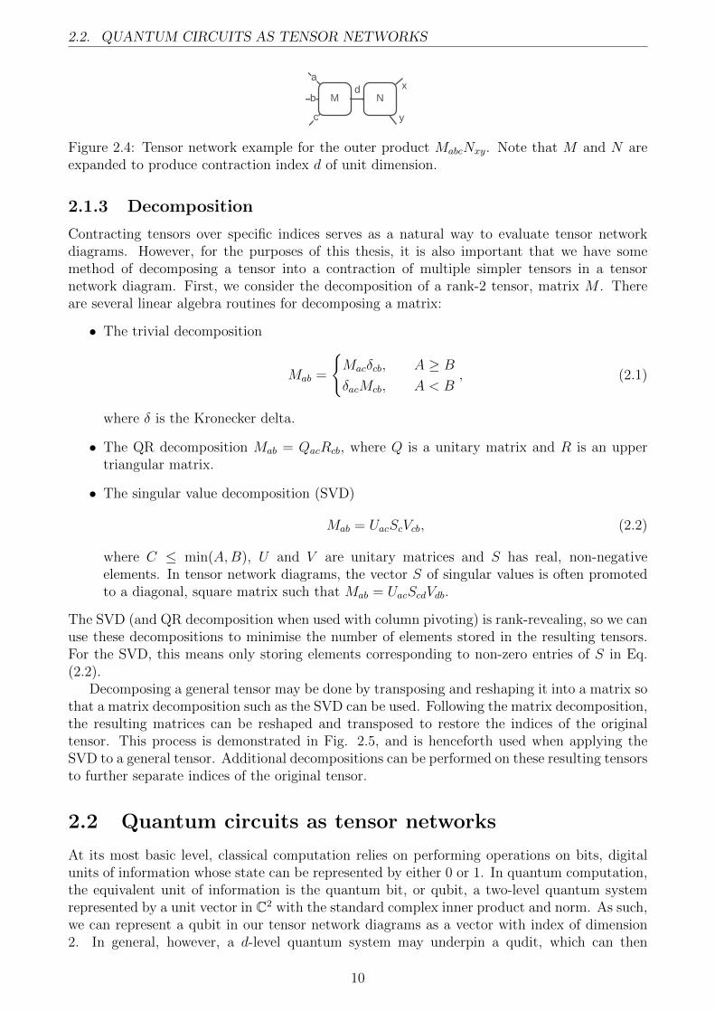
A tensor product T of two tensors A and B has the combined indices of A and B suchthat each element of T is the scalar product of the element in A and the element in B withthe corresponding indices. For example, the outer product of two vectors yields Tab = AaBb.Pictorially, this can be thought of as reshaping both A and B to add a new index of unitdimension and contracting over this new index. An addition example is provided in Fig. 2.4.
9
2.2. QUANTUM CIRCUITS AS TENSOR NETWORKS
Mb
c
N
y
xda
Figure 2.4: Tensor network example for the outer product MabcNxy. Note that M and N areexpanded to produce contraction index d of unit dimension.
2.1.3 Decomposition
Contracting tensors over specific indices serves as a natural way to evaluate tensor networkdiagrams. However, for the purposes of this thesis, it is also important that we have somemethod of decomposing a tensor into a contraction of multiple simpler tensors in a tensornetwork diagram. First, we consider the decomposition of a rank-2 tensor, matrix M . Thereare several linear algebra routines for decomposing a matrix:
• The trivial decomposition
Mab =
{Macδcb, A ≥ B
δacMcb, A < B, (2.1)
where δ is the Kronecker delta.
• The QR decomposition Mab = QacRcb, where Q is a unitary matrix and R is an uppertriangular matrix.
• The singular value decomposition (SVD)
Mab = UacScVcb, (2.2)
where C ≤ min(A,B), U and V are unitary matrices and S has real, non-negativeelements. In tensor network diagrams, the vector S of singular values is often promotedto a diagonal, square matrix such that Mab = UacScdVdb.
The SVD (and QR decomposition when used with column pivoting) is rank-revealing, so we canuse these decompositions to minimise the number of elements stored in the resulting tensors.For the SVD, this means only storing elements corresponding to non-zero entries of S in Eq.(2.2).
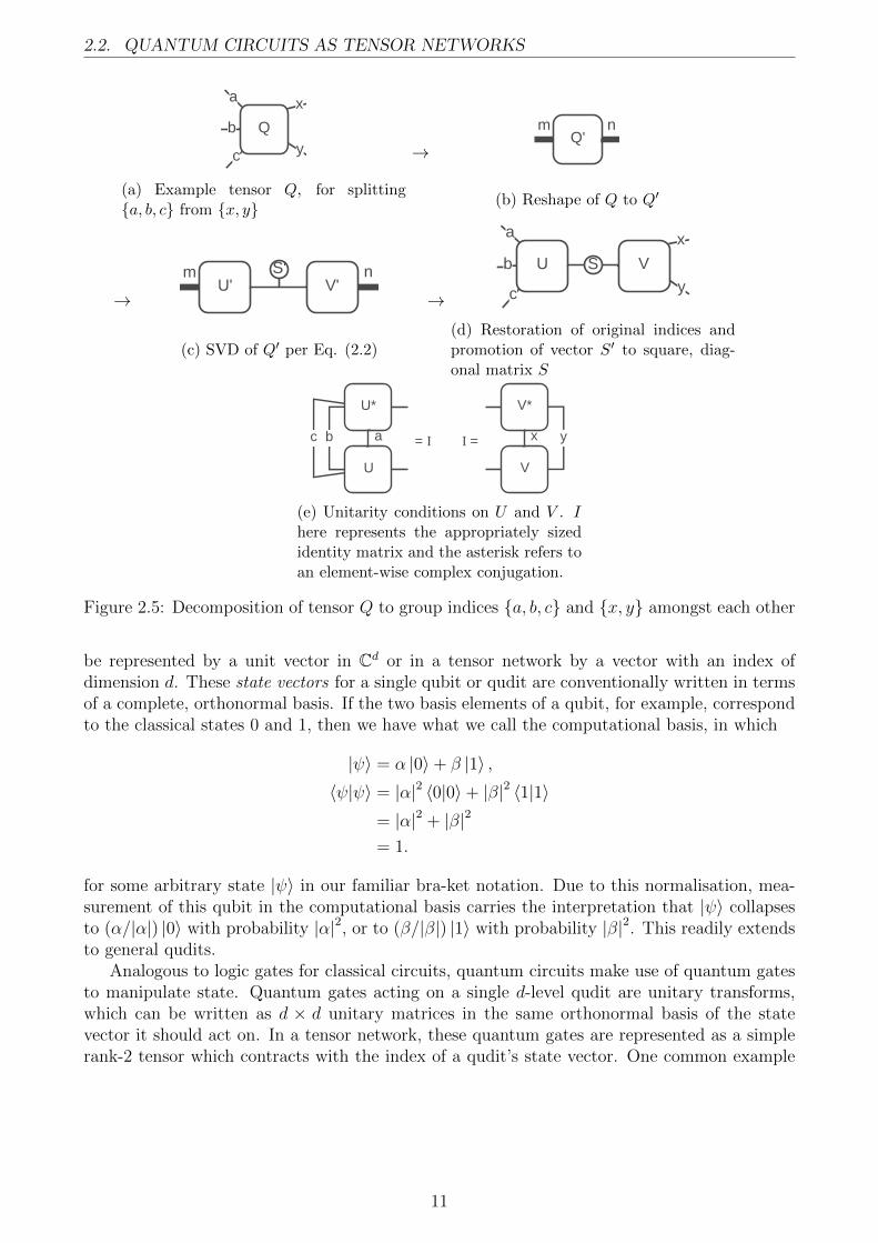
Decomposing a general tensor may be done by transposing and reshaping it into a matrix sothat a matrix decomposition such as the SVD can be used. Following the matrix decomposition,the resulting matrices can be reshaped and transposed to restore the indices of the originaltensor. This process is demonstrated in Fig. 2.5, and is henceforth used when applying theSVD to a general tensor. Additional decompositions can be performed on these resulting tensorsto further separate indices of the original tensor.
2.2 Quantum circuits as tensor networks
At its most basic level, classical computation relies on performing operations on bits, digitalunits of information whose state can be represented by either 0 or 1. In quantum computation,the equivalent unit of information is the quantum bit, or qubit, a two-level quantum systemrepresented by a unit vector in C2 with the standard complex inner product and norm. As such,we can represent a qubit in our tensor network diagrams as a vector with index of dimension2. In general, however, a d-level quantum system may underpin a qudit, which can then
10
2.2. QUANTUM CIRCUITS AS TENSOR NETWORKS
Qb
c
a x
y
(a) Example tensor Q, for splitting{a, b, c} from {x, y}
→Q'
m n
(b) Reshape of Q to Q′
→U'
mV'
nS'
(c) SVD of Q′ per Eq. (2.2)
→
SUb
c
a
V
x
y
(d) Restoration of original indices andpromotion of vector S′ to square, diag-onal matrix S
U
U*
bc a = I
V
V*
xI = y
(e) Unitarity conditions on U and V . Ihere represents the appropriately sizedidentity matrix and the asterisk refers toan element-wise complex conjugation.
Figure 2.5: Decomposition of tensor Q to group indices {a, b, c} and {x, y} amongst each other
be represented by a unit vector in Cd or in a tensor network by a vector with an index ofdimension d. These state vectors for a single qubit or qudit are conventionally written in termsof a complete, orthonormal basis. If the two basis elements of a qubit, for example, correspondto the classical states 0 and 1, then we have what we call the computational basis, in which
|ψ〉 = α |0〉+ β |1〉 ,〈ψ|ψ〉 = |α|2 〈0|0〉+ |β|2 〈1|1〉
= |α|2 + |β|2
= 1.
for some arbitrary state |ψ〉 in our familiar bra-ket notation. Due to this normalisation, mea-surement of this qubit in the computational basis carries the interpretation that |ψ〉 collapsesto (α/|α|) |0〉 with probability |α|2, or to (β/|β|) |1〉 with probability |β|2. This readily extendsto general qudits.
Analogous to logic gates for classical circuits, quantum circuits make use of quantum gatesto manipulate state. Quantum gates acting on a single d-level qudit are unitary transforms,which can be written as d × d unitary matrices in the same orthonormal basis of the statevector it should act on. In a tensor network, these quantum gates are represented as a simplerank-2 tensor which contracts with the index of a qudit’s state vector. One common example
11
2.2. QUANTUM CIRCUITS AS TENSOR NETWORKS
of a quantum gate is the Hadamard gate for qubits, which performs the operation
H |0〉 =1√2
(|0〉+ |1〉),
H |1〉 =1√2
(|0〉 − |1〉).
As such, the Hadamard gate has a matrix representation
H =1√2
[1 11 −1
](2.3)
in the computational basis.In a system of multiple qudits, the set of basis vectors of the overall state vector is the set
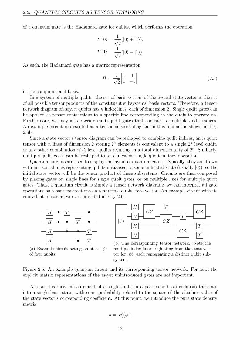
of all possible tensor products of the constituent subsystems’ basis vectors. Therefore, a tensornetwork diagram of, say, n qubits has n index lines, each of dimension 2. Single qudit gates canbe applied as tensor contractions to a specific line corresponding to the qudit to operate on.Furthermore, we may also operate multi-qudit gates that contract to multiple qudit indices.An example circuit represented as a tensor network diagram in this manner is shown in Fig.2.6b.
Since a state vector’s tensor diagram can be reshaped to combine qudit indices, an n qubittensor with n lines of dimension 2 storing 2n elements is equivalent to a single 2n level qudit,or any other combination of di level qudits resulting in a total dimensionality of 2n. Similarly,multiple qudit gates can be reshaped to an equivalent single qudit unitary operation.
Quantum circuits are used to display the layout of quantum gates. Typically, they are drawnwith horizontal lines representing qubits initialised to some indicated state (usually |0〉), so theinitial state vector will be the tensor product of these subsystems. Circuits are then composedby placing gates on single lines for single qubit gates, or on multiple lines for multiple qubitgates. Thus, a quantum circuit is simply a tensor network diagram: we can interpret all gateoperations as tensor contractions on a multiple-qubit state vector. An example circuit with itsequivalent tensor network is provided in Fig. 2.6.
H • T •
H • • T •
H • • T
H • T
(a) Example circuit acting on state |ψ〉of four qubits
|ψ〉
HCZ
TCZ
HCZ
T
HCZ
T
H T
(b) The corresponding tensor network. Note themultiple index lines originating from the state vec-tor for |ψ〉, each representing a distinct qubit sub-system.
Figure 2.6: An example quantum circuit and its corresponding tensor network. For now, theexplicit matrix representations of the as-yet unintroduced gates are not important.
As stated earlier, measurement of a single qudit in a particular basis collapses the stateinto a single basis state, with some probability related to the square of the absolute value ofthe state vector’s corresponding coefficient. At this point, we introduce the pure state densitymatrix
ρ = |ψ〉〈ψ| .
12

2.3. MATRIX PRODUCT STATES
In a tensor network, we construct this density matrix by taking the tensor product of a statevector with its complex conjugate. The diagonal elements of this density matrix now indicatethe probability of measuring a particular state. The density matrix for a system of multiplequdits, by extension, is the tensor product of a multiple-qudit state vector with its complexconjugate, shown in Fig. 2.7a.
In a system of multiple qudits, measurement of a single qudit also requires the density matrixof the entire state vector. However, in order to arrive at a reduced density matrix for the quditsystem to be measured, we now ‘trace over’ all other qudit subsystems by contracting pairsof index lines corresponding to each other qudit (so that the only free indices of the reduceddensity matrix correspond to the qudit of interest) as per Fig. 2.7b. The diagonal elements ofthis reduced density matrix correspond to the probabilities pm of measuring value m from thequdit. When a particular value m is measured for the given qudit, all elements in the originalstate vector corresponding to m for that qudit are rescaled by 1/
√pm, and all other elements
are set to zero. In this way, we can also interpret measurements of single qubits in quantumcircuit diagrams.
? ? *
?=
(a) Tensor network of the pure densitymatrix ρ = |ψ〉〈ψ|, where the contractedindex has unit dimension
?
(b) The reduced density matrix of thesecond qudit system.
Figure 2.7: Tensor networks for the density matrix and reduced density matrix
2.3 Matrix Product States
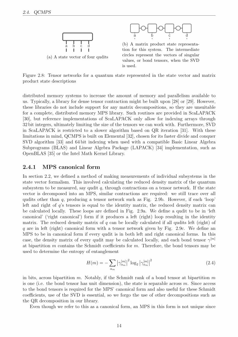
In contrast to a state vector simulation of a quantum circuit, which performs gate operationsas tensor contractions on the entire state vector (of size 2n for an n qubit system), the matrixproduct state (MPS) formalism was developed for its adaptive computational resource require-ments, and also allows simulating gates as local operations. To accomplish this, the state vectortensor is sequentially decomposed so that each qudit line is joined to a distinct tensor which arelaid out linearly, producing a tensor network like Fig. 2.8b. Therefore, each tensor in an MPSchain has three index lines: one representing the qudit’s index in the original state vector, andindex lines to the left and right contracting to adjacent qudits. Applying single qudit gates nowonly requires contraction with the relevant qudit tensors rather than the entire state vector. Ifthe SVD, Eq. (2.2), is used as the matrix decomposition, we also have the vectors of singularvalues between each qudit tensor. We refer to these vectors as the bond tensors, and althoughthey can be contracted into an adjacent qudit tensor, we choose to keep them separate. Whywe choose to do so will be explained shortly.
In the following section, we demonstrate the mechanics of the MPS formalism as operationsperformed by our numerical library QCMPS.
2.4 QCMPS
We have developed a C++ library titled QCMPS for applying the MPS formalism specificallyto simulating quantum circuits. Due to the limited computational resources of a single classicalcomputer, we require the use of the Message Passing Interface (MPI) [27] to make use of
13
2.4. QCMPS
a b c d
(a) A state vector of four qudits
a b c d
(b) A matrix product state representa-tion for this system. The intermediatecircles represent the vectors of singularvalues, or bond tensors, when the SVDis used.
Figure 2.8: Tensor networks for a quantum state represented in the state vector and matrixproduct state descriptions
distributed memory systems to increase the amount of memory and parallelism available tous. Typically, a library for dense tensor contraction might be built upon [28] or [29]. However,these libraries do not include support for any matrix decompositions, so they are unsuitablefor a complete, distributed memory MPS library. Such routines are provided in ScaLAPACK[30], but reference implementations of ScaLAPACK only allow for indexing arrays through32 bit integers, ultimately limiting the size of the tensors we can work with. Furthermore, SVDin ScaLAPACK is restricted to a slower algorithm based on QR iteration [31]. With theselimitations in mind, QCMPS is built on Elemental [32], chosen for its faster divide and conquerSVD algorithm [33] and 64 bit indexing when used with a compatible Basic Linear AlgebraSubprograms (BLAS) and Linear Algebra Package (LAPACK) [34] implementation, such asOpenBLAS [35] or the Intel Math Kernel Library.
2.4.1 MPS canonical form
In section 2.2, we defined a method of making measurements of individual subsystems in thestate vector formalism. This involved calculating the reduced density matrix of the quantumsubsystem to be measured, say qudit q, through contractions on a tensor network. If the statevector is decomposed into an MPS, similar contractions are required: we still trace over allqudits other than q, producing a tensor network such as Fig. 2.9b. However, if each ‘loop’left and right of q’s tensors is equal to the identity matrix, the reduced density matrix canbe calculated locally. These loops are defined in Fig. 2.9a. We define a qudit to be in ‘leftcanonical’ (‘right canonical’) form if it produces a left (right) loop resulting in the identitymatrix. The reduced density matrix of q can be locally calculated if all qudits left (right) ofq are in left (right) canonical form with a tensor network given by Fig. 2.9c. We define anMPS to be in canonical form if every qudit is in both left and right canonical forms. In thiscase, the density matrix of every qudit may be calculated locally, and each bond tensor γ[m]
at bipartition m contains the Schmidt coefficients for m. Therefore, the bond tensors may beused to determine the entropy of entanglement
H(m) = −∑αm
∣∣γ[m]αm
∣∣2 log2
∣∣γ[m]αm
∣∣2 (2.4)
in bits, across bipartition m. Notably, if the Schmidt rank of a bond tensor at bipartition mis one (i.e. the bond tensor has unit dimension), the state is separable across m. Since accessto the bond tensors is required for the MPS’ canonical form and also useful for these Schmidtcoefficients, use of the SVD is essential, so we forgo the use of other decompositions such asthe QR decomposition in our library.
Even though we refer to this as a canonical form, an MPS in this form is not unique since
14

2.4. QCMPS
?[i]?[i-1]
?[i]*?[i-1]
?[i] ?[i]
?[i]* ?[i]
= I I =
(a) Left and right canonicalisation conditions for a qudit iwhose MPS tensor is labelled Γ[i]. Matrices I here are theappropriately sized identities.
?[1] ?[2]?[1] ?[3] ?[4]?[3]?[2]
?[1]* ?[2]*?[1] ?[3]* ?[4]*?[3]?[2]
(b) The reduced density matrix obtainedby combining Figs. 2.7a, 2.7b and 2.8b.
?[2]?[1] ?[2]
?[2]*?[1] ?[2]
(c) The reduced density matrix from Fig.2.9b if qudits i < 2 (i > 2) are in left(right) canonical form, per Fig. 2.9a.
Figure 2.9: The MPS canonicalisation conditions and their implications for the reduced densitymatrix. If a qudit is at the ends of the MPS, any missing bond tensors may be omitted fromFigs. 2.9a and 2.9c.
the SVD itself is not unique. One such example is the trivially separable two qudit state
|0〉 ⊗ |0〉 =(eiθ |0〉
)⊗(e−iθ |0〉
),
which has different coefficients in the equivalent canonical expressions. This point is noted asan error in [36].
2.4.2 Contraction and decomposition
The contraction operation allows us to combine two adjacent qudits with dimensions d1 and d2into a single effective qudit of dimension d1d2. This is akin to a simple reshape of a state vector’stensor. To perform this operation, both qudit tensors are reshaped into matrices where onematrix index corresponds to the resulting free indices and the other index corresponds to thecontraction indices. This initial reshape allows us to make use of optimised BLAS routines formatrix multiplication instead of slower nested loops, a choice determined on behalf of our testingand in agreement with recommendations made in [37]. The intermediate bond tensor is thencontracted into the smaller of the left or right qudit’s reshaped tensor to save computation time.Matrix multiplication is then performed on the two reshaped qudit tensors, and the resultingmatrix is reshaped into a tensor for a qudit of dimension d1d2. Importantly, if both qudits arein left (right) canonical form, the contracted qudit is also in left (right) canonical form. Hence,contraction maintains an MPS’ canonicalisation.
Decomposition is the reverse operation of contraction, and aims to decompose a qudit ofdimension d1d2 into a left qudit of dimension d1 and a right qudit of dimension d2. To performa decomposition, any existing adjacent bond tensors are first contracted into the qudit tensor.The qudit tensor is then reshaped into a matrix where one index combines the left bond indexand the left subsystem’s index of dimension d1, and the other combines the right bond index
15
2.4. QCMPS
and right subsystem’s index of dimension d2. We can then perform the SVD, Eq. (2.2), tothis matrix. Since the SVD is rank revealing, we can take an opportunity here to only keeptensor elements corresponding to non-zero singular values. Notably, since the bond tensorscorrespond to the Schmidt coefficients across the corresponding bipartition, storing only non-zero singular values allows the space requirements of a canonical MPS to scale with the amountof entanglement across each bipartition. Numerically, we only consider singular values of m×nmatrix A above
ε‖A‖2 max(m,n) (2.5)
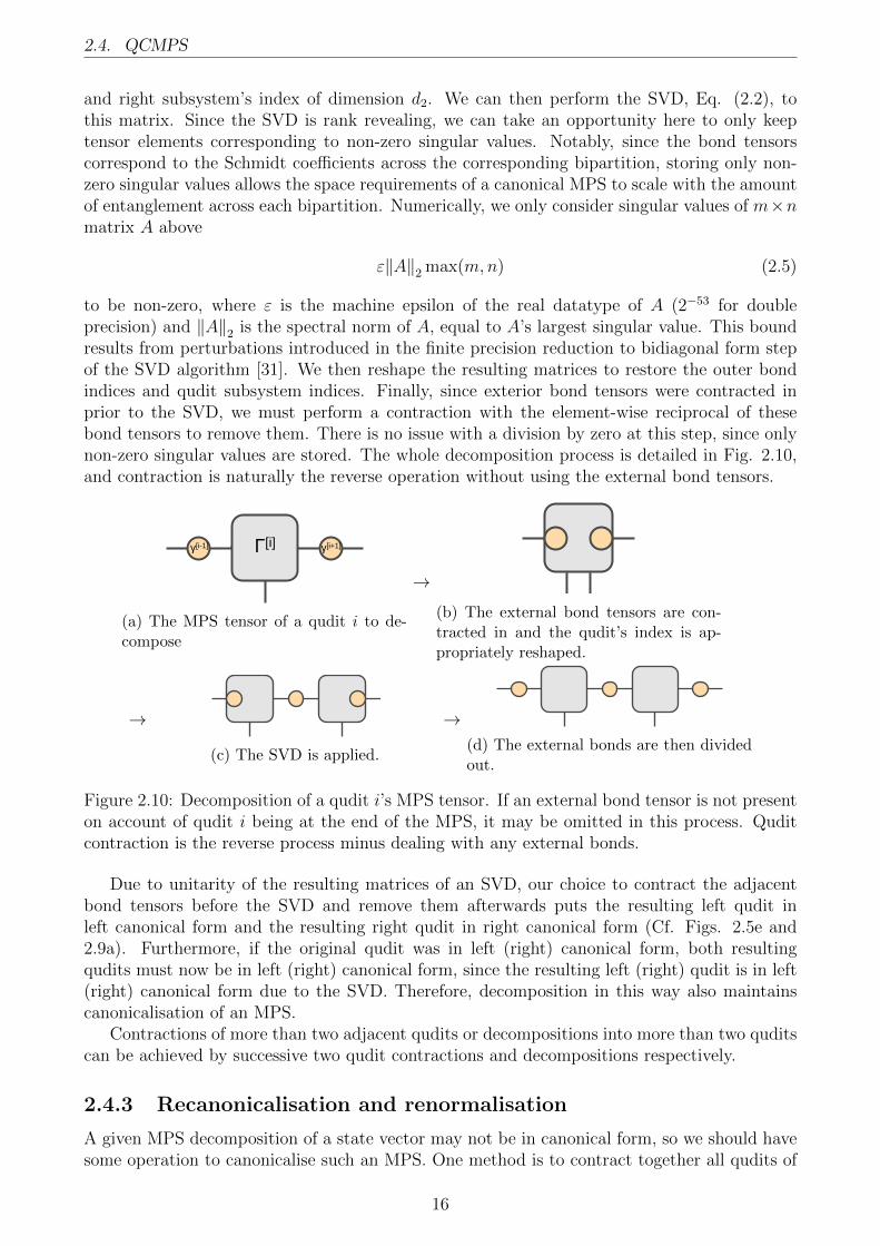
to be non-zero, where ε is the machine epsilon of the real datatype of A (2−53 for doubleprecision) and ‖A‖2 is the spectral norm of A, equal to A’s largest singular value. This boundresults from perturbations introduced in the finite precision reduction to bidiagonal form stepof the SVD algorithm [31]. We then reshape the resulting matrices to restore the outer bondindices and qudit subsystem indices. Finally, since exterior bond tensors were contracted inprior to the SVD, we must perform a contraction with the element-wise reciprocal of thesebond tensors to remove them. There is no issue with a division by zero at this step, since onlynon-zero singular values are stored. The whole decomposition process is detailed in Fig. 2.10,and contraction is naturally the reverse operation without using the external bond tensors.
?[i]?[i-1] ?[i+1]
(a) The MPS tensor of a qudit i to de-compose
→(b) The external bond tensors are con-tracted in and the qudit’s index is ap-propriately reshaped.
→
(c) The SVD is applied.
→(d) The external bonds are then dividedout.
Figure 2.10: Decomposition of a qudit i’s MPS tensor. If an external bond tensor is not presenton account of qudit i being at the end of the MPS, it may be omitted in this process. Quditcontraction is the reverse process minus dealing with any external bonds.
Due to unitarity of the resulting matrices of an SVD, our choice to contract the adjacentbond tensors before the SVD and remove them afterwards puts the resulting left qudit inleft canonical form and the resulting right qudit in right canonical form (Cf. Figs. 2.5e and2.9a). Furthermore, if the original qudit was in left (right) canonical form, both resultingqudits must now be in left (right) canonical form, since the resulting left (right) qudit is in left(right) canonical form due to the SVD. Therefore, decomposition in this way also maintainscanonicalisation of an MPS.
Contractions of more than two adjacent qudits or decompositions into more than two quditscan be achieved by successive two qudit contractions and decompositions respectively.
2.4.3 Recanonicalisation and renormalisation
A given MPS decomposition of a state vector may not be in canonical form, so we should havesome operation to canonicalise such an MPS. One method is to contract together all qudits of
16
2.4. QCMPS
the MPS, effectively producing a state vector tensor, and then to sequentially decompose thisstate vector back into individual qudits. However, by operating on a full state vector in thisintermediate step, we lose any space advantage afforded to us by an MPS representation witha rank revealing decomposition.
A more promising method of recanonicalising a general MPS that mitigates this memorycost is to perform pairwise qudit contractions and decompositions from one end of the MPSto the other end and back. We refer to a series of pairwise contractions and decompositionsas a sweep, so recanonicalisation can be achieved via a sweep from the left end to the rightend and back or vice-versa. Since a decomposition puts the left (right) qudit in left (right)canonical form, a right (left) sweep from the left (right) end puts every qubit except potentiallythe rightmost (leftmost) qudit in left (right) canonical form. However, this rightmost (leftmost)qudit is guaranteed to be in left (right) canonical form if the entire state is normalised correctlyto 〈ψ|ψ〉 = 1. Since we only work on pairs of qudits at a time, we do not incur as great amemory cost as contracting into an entire state vector.
If a state is not normalised correctly or becomes unnormalised (possibly due to a build upof numeric imprecision), we can still perform a complete left and right sweep to produce anMPS in an unnormalised canonical form. In this form, a bond tensor λ[m] at bipartition m stillcontains the Schmidt coefficients of m, but their squares no longer sum to one:∑
αm
∣∣γ[m]αm
∣∣2 = 〈ψ|ψ〉
6= 1.
Therefore, we should first rescale the bond tensor for each bipartition m via
γ[m]αm← γ
[m]αm√〈ψ|ψ〉
.
To produce the correct overall normalisation, qudit tensor Γ[q] for each interior qudit q (i.e. qis not at an end of the MPS chain) is updated via
Γ[q]iqαqαq+1
← Γ[q]iqαqαq+1
√〈ψ|ψ〉,
where iq is the qudit index, αq is the left bond index and αq+1 is the right bond index. Sincethere is exactly one more bond than there is interior qudit, the overall affect of these rescalingsis to take
|ψ〉 ← |ψ〉√〈ψ|ψ〉
,
thus normalising and canonicalising the MPS correctly. Furthermore, these rescalings do notrequire any MPI communication (apart from initially determining 〈ψ|ψ〉 from a bond in anunnormalised canonical MPS) and are easily vectorised, so this extra normalisation step hasminimal time overhead.
2.4.4 Truncation
We have established that the use of the rank revealing SVD allows a space advantage for acanonical MPS representation of a quantum state with low Schmidt rank (i.e. low entanglement)across each bipartition when compared to the full state vector. If we consider some bond m ina canonical MPS and contract all qudits left of m into subsystem A and all qudits right of m
17
2.4. QCMPS
into subsystem B, we arrive at the Schmidt decomposition
|ψ〉 =
χ∑αm=1
γ[m]αm
∣∣Γ[A]αm
⟩⊗∣∣Γ[B]
αm
⟩, (2.6)
where χ is the numerical Schmidt rank across m, remembering that we only chose to considertensor elements corresponding to non-zero singular values according to the threshold definedin Eq. (2.5). Numerical implementations of the SVD produce the (non-negative, real) singular
values in descending order, so we let γ[m]αm decrease with αm. Therefore, the Schmidt decomposi-
tion in Eq. (2.6) with decreasing singular values γ[m]αm , gives rise to a natural lossy compression
scheme to approximate the state |ψ〉 by extending the sum to some compressed Schmidt rankξ < χ. In the context of an MPS, this process of reducing a bond’s dimension is referred to asa truncation. It produces an MPS with smaller memory requirements at the cost of fidelity tothe original state. We also note that truncation in this manner requires the use of the SVD toprovide access to the Schmidt coefficients through the singular values.
Directly following the truncation of a bond between left qudit q1 and right qudit q2, q1 is nolonger in right canonical form and q2 is no longer in left canonical form. The whole MPS canbe returned to a canonical form by performing a left sweep from q1 and a right sweep from q2.However, this canonical form is unnormalised, since truncation of the bond between q1 and q2removes some Schmidt coefficients. We can apply a renormalisation at this point to produce acanonical MPS with correct normalisation.
It is important to note that truncation to a canonical MPS is not a purely local operation,i.e. one involving the two qudits adjacent to the truncated bond. Truncation of a bond ofSchmidt rank χ to a truncated rank ξ can be thought of as receiving
|ψtrunc〉 =
ξ<χ∑αm=1
γ[m]αm
∣∣Γ[A]αm
⟩⊗∣∣Γ[B]
αm
⟩as the result of some measurement (before renormalisation). Since a measurement should ingeneral serve to collapse entanglement throughout a state, sweeps outward from the truncatedbond are required to propagate this collapse. Numerical tests show that renormalising thetruncated bond alone, as erroneously suggested in [36], is not enough to renormalise, let alonerecanonicalise an MPS.
Canonicalised truncation in this method is a per-bond operation. If entanglement is intro-duced into multiple bonds simultaneously (perhaps through the application of a gate operationon multiple qudits as per subsection 2.4.6) through an increase in the Schmidt ranks, the usermust choose some ordering of these bonds to perform canonicalised truncations on. We alsoprovide the option of performing an uncanonicalised truncation, where bonds can simply betruncated and the recanonicalisation sweeps and renormalisation operation can be applied justprior to some operation requiring a canonical MPS.
2.4.5 Measurement and reset
Measurement is the method by which we extract any results from a quantum algorithm run-ning on a quantum computer. In section 2.2, we required the reduced density matrix of a quditsubsystem in order to measure it. Furthermore, in subsection 2.4.1, we showed how canon-icalisation allows us to calculate a qudit’s reduced density matrix locally. Combining thesepoints, the first step of performing a measurement of qudit q is to ensure that every qudit left(right) of q is in left (right) canonical form. This is automatically the case if the MPS is incanonical form, but can be achieved by sweeping inward from the ends at least up to q. We
18
2.4. QCMPS
can then calculate the diagonal elements pm of the reduced density matrix of q locally. Sincethe pm correspond to probabilities of measuring value m from qudit q, we can sample from thisdiscrete distribution to simulate a measurement result of some value m.
To put the MPS into a state where m was measured from qudit q, we temporarily shrinkq to a one dimensional qudit subsystem corresponding to the measured value m with correctnormalisation. That is, if m is the result of our measurement, we project
Γ[q]αqαq+1
← Γ[q]mαqαq+1√pm
. (2.7)
Since qudits left (right) of q were already in left (right) canonical form prior to this projection,we only need to perform sweeps outward from q in both directions to canonicalise the MPS (ifwe wish to canonicalise it). Since measurement collapses entanglement throughout the state,these outward sweeps serve to propagate this collapse of entanglement, in a similar fashion tothe outward sweeps of truncation.
We chose to shrink q to a qudit of dimension one prior to the sweeps to avoid contractionand decomposition operations using a tensor that would otherwise have zeros for each elementnot corresponding to m. This method results in exceptional time and space savings, especiallyif the dimensionality of q was very large (i.e. if q consists of many qubits). However, since aone level qudit subsystem is not computationally useful, we must expand q’s tensor back to fulldimensionality if q is to be used in further operations. That is, we update q’s tensor so that
Γ[q]iqαqαq+1
←
{Γ[q]αqαq+1 , iq = m
0, iq 6= m. (2.8)
Otherwise, if q is not needed for further operations, we can contract the unexpanded, onedimensional qudit q into an adjacent qudit, effectively removing it since the measurementmakes q separable from the rest of the system. We choose to contract into the adjacent quditwith the smaller tensor to minimise computation time.
If we wish to reset a qudit q to a certain value s, we perform an unexpanded qudit measure-ment of q with or without the subsequent canonicalisation, producing measurement result m.We then perform some classical switching on q that maps |m〉 → |s〉. This can be accomplishedvia an alternate expansion to Eq. (2.8) where the unexpanded tensor for m is placed into s:
Γ[q]iqαqαq+1
←
{Γ[q]αqαq+1 , iq = s
0, iq 6= s,
following from Eq. (2.7).
2.4.6 Gate operations
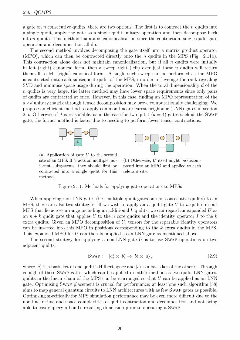
In order to simulate quantum circuits, we must be able to apply quantum gates to our MPS.As mentioned in section 2.2, quantum gates are unitary operations that contract onto a statevector when applied. For single qudit gates, the generalisation to an MPS is simple: the gate’sunitary matrix in the computational basis is simply contracted to the specified qudit’s tensor,whilst maintaining any left or right canonicalisation of the qudit and hence any canonicalisationof the entire MPS. The schematic for this process is given by Fig. 2.11a.
Gates on multiple qudits are easily applied to a state vector through tensor contraction andappropriate index bookkeeping. Since an MPS lays the qudit tensors out in a linear chain, it ismost straightforward to apply a multiple qudit gate to consecutive qudits on an MPS. To apply
19
2.4. QCMPS
a gate on n consecutive qudits, there are two options. The first is to contract the n qudits intoa single qudit, apply the gate as a single qudit unitary operation and then decompose backinto n qudits. This method maintains canonicalisation since the contraction, single qudit gateoperation and decomposition all do.
The second method involves decomposing the gate itself into a matrix product operator(MPO), which can then be contracted directly onto the n qudits in the MPS (Fig. 2.11b).This contraction alone does not maintain canonicalisation, but if all n qudits were initiallyin left (right) canonical form, then a sweep right (left) over just these n qudits will returnthem all to left (right) canonical form. A single such sweep can be performed as the MPOis contracted onto each subsequent qudit of the MPS, in order to leverage the rank revealingSVD and minimise space usage during the operation. When the total dimensionality d of then qudits is very large, the latter method may have lower space requirements since only pairsof qudits are contracted at once. However, in this case, finding an MPO representation of thed×d unitary matrix through tensor decomposition may prove computationally challenging. Wepropose an efficient method to apply common linear nearest neighbour (LNN) gates in section2.5. Otherwise if d is reasonable, as is the case for two qubit (d = 4) gates such as the Swapgate, the former method is faster due to needing to perform fewer tensor contractions.
U
(a) Application of gate U to the secondsite of an MPS. If U acts on multiple, ad-jacent subsystems, they should first becontracted into a single qudit for thismethod.
(b) Otherwise, U itself might be decom-posed into an MPO and applied to eachrelevant site.
Figure 2.11: Methods for applying gate operations to MPSs
When applying non-LNN gates (i.e. multiple qudit gates on non-consecutive qudits) to anMPS, there are also two strategies. If we wish to apply an n qudit gate U to n qudits in ourMPS that lie across a range including an additional k qudits, we can regard an expanded U asan n + k qudit gate that applies U to the n core qudits and the identity operator I to the kextra qudits. Given an MPO decomposition of U , tensors for the separable identity operatorscan be inserted into this MPO in positions corresponding to the k extra qudits in the MPS.This expanded MPO for U can then be applied as an LNN gate as mentioned above.
The second strategy for applying a non-LNN gate U is to use Swap operations on twoadjacent qudits
Swap : |a〉 ⊗ |b〉 → |b〉 ⊗ |a〉 , (2.9)
where |a〉 is a basis ket of one qudit’s Hilbert space and |b〉 is a basis ket of the other’s. Throughenough of these Swap gates, which can be applied in either method as two-qudit LNN gates,qudits in the linear chain of the MPS can be rearranged so that U can be applied as an LNNgate. Optimising Swap placement is crucial for performance; at least one such algorithm [38]aims to map general quantum circuits to LNN architectures with as few Swap gates as possible.Optimising specifically for MPS simulation performance may be even more difficult due to thenon-linear time and space complexities of qudit contraction and decomposition and not beingable to easily query a bond’s resulting dimension prior to operating a Swap.
20
2.5. GENERAL CONTROLLED GATE OPERATIONS FOR MPS
2.5 General controlled gate operations for MPS
One of the most common multiple qudit gate structures is the controlled gate operation. Con-sider first a single qubit gate such as the X gate
|0〉 → |1〉 ,|1〉 → |0〉 ,
the quantum equivalent of the classical Not gate in the computational basis. A controlled Xgate, otherwise known as the CNot gate, applies the X gate to a qubit based on the state ofanother:
|0〉 ⊗ |0〉 → |0〉 ⊗ |0〉 ,|0〉 ⊗ |1〉 → |0〉 ⊗ |1〉 ,|1〉 ⊗ |0〉 → |1〉 ⊗ |1〉 ,|1〉 ⊗ |1〉 → |1〉 ⊗ |0〉 .
Here, the state of the first qubit is used to conditionally apply the X gate on the second qubit:if the first qubit is in the |1〉 state, then the X gate is applied to the second qubit; otherwisethe identity operation is applied to the second qubit. The state of the control qubit is leftunchanged. This is a form of binary control, where each state for a control qudit is individuallyeither ‘on’ or ‘off’, specifying whether or not to apply the attached gate. For example, a five-level control qudit might apply the main gate operation in states |0〉, |2〉 or |4〉, whilst applyingthe identity in states |1〉 or |3〉. When there are multiple binary control qudits, the main gateoperation is only applied when all control qudits are in an ‘on’ state. If there are multiplesimultaneously controlled gate operations, they are treated as a single operation: that is, ifthe control qudits take an ‘on’ state, then all attached gate operations are applied to theirrespective qudits. Otherwise, if any control qudit takes an ‘off’ state, none of the attachedgates are applied.
For an MPS, we are interested in being able to apply LNN restricted versions of these generalbinarily controlled gate operations. Specifically, we require that not only the entire controlledgate operation be LNN, but also that the main gates (i.e. the gates binarily controlled by thecontrol qudits) be LNN. Fig. 2.12 contains an example of such a gate. If the main gates areeach LNN but the control qudits cause the entire gate structure not to be LNN, identity gateoperations I can be inserted at each qudit gap. In this way, we may simulate, for example,a CNot gate on distant qubits as a controlled I ⊗ . . . ⊗ I ⊗ X gate. However, this does notprovide a simple method of applying a long range Swap (Eq. (2.9)) to two qudits.
To review the options detailed in subsection 2.4.6 of applying a gate to an MPS, we couldeither contract the required qudits into a single qudit that we then apply the gate to, ordecompose a matrix representation of the gate into an MPO and contract that onto the MPS.Both methods have space limitations when the total dimensionality of the required qudits isvery large: the former in contracting the qudits together and the latter in decomposing a largematrix representing the gate operation. However, it is possible to apply an LNN generalisedbinarily controlled gate (LNNGBCG) whilst avoiding complete qudit contraction or operatordecomposition.
We propose the following rules for obtaining a resulting MPS after such an LNNGBCG isapplied. From these, an MPO representation of the gate can easily be obtained. We requirethat any main gates are applied as single qudit operations: for example, a two qubit Swaprequires the two adjacent qubits be contracted. Moreover, in the interest of space and timeusage, the following traits are desirable:
21
2.5. GENERAL CONTROLLED GATE OPERATIONS FOR MPS
•
H
X
×
×
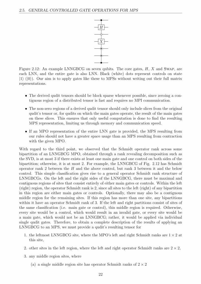
•Figure 2.12: An example LNNGBCG on seven qubits. The core gates, H, X and Swap, areeach LNN, and the entire gate is also LNN. Black (white) dots represent controls on state|1〉 (|0〉). Our aim is to apply gates like these to MPSs without writing out their full matrixrepresentations.
• The derived qudit tensors should be block sparse whenever possible, since zeroing a con-tiguous region of a distributed tensor is fast and requires no MPI communication.
• The non-zero regions of a derived qudit tensor should only include slices from the originalqudit’s tensor or, for qudits on which the main gates operate, the result of the main gateson these slices. This ensures that only useful computation is done to find the resultingMPS representation, limiting us through memory and communication speed.
• If an MPO representation of the entire LNN gate is provided, the MPS resulting fromour rules should not have a greater space usage than an MPS resulting from contractionwith the given MPO.
With regard to the third point, we observed that the Schmidt operator rank across somebipartition of an LNNGBCG MPO, obtained through a rank revealing decomposition such asthe SVD, is at most 3 if there exists at least one main gate and one control on both sides of thebipartition; otherwise, it is at most 2. For example, the LNNGBCG of Fig. 2.12 has Schmidtoperator rank 2 between the H and the above control, but rank 3 between it and the belowcontrol. This simple classification gives rise to a general operator Schmidt rank structure ofLNNGBCGs. On the left and the right sides of the LNNGBCG, there must be maximal andcontiguous regions of sites that consist entirely of either main gates or controls. Within the left(right) region, the operator Schmidt rank is 2, since all sites to the left (right) of any bipartitionin this region are either main gates or controls. Optionally, there may also be a contiguousmiddle region for the remaining sites. If this region has more than one site, any bipartitionswithin it have an operator Schmidt rank of 3. If the left and right partitions consist of sites ofthe same classification (i.e. main gate or control), this middle region is required. Otherwise,every site would be a control, which would result in an invalid gate, or every site would bea main gate, which would not be an LNNGBCG; rather, it would be applied via individualsingle qudit gates. Therefore, to obtain a complete description of the results of applying anLNNGBCG to an MPS, we must provide a qudit’s resulting tensor for
1. the leftmost LNNGBCG site, where the MPO’s left and right Schmidt ranks are 1× 2 atthis site,
2. other sites in the left region, where the left and right operator Schmidt ranks are 2× 2,
3. any middle region sites, where
(a) a single middle region site has operator Schmidt ranks of 2× 2
22
2.5. GENERAL CONTROLLED GATE OPERATIONS FOR MPS
(b) or if there are multiple middle region sites,
i. the leftmost site of the middle region has ranks 2× 3,
ii. any interior sites of the middle region has ranks 3× 3 and
iii. the middle region’s rightmost site has ranks 3× 2,
4. other sites of the right region, with ranks 2× 2, and finally
5. the rightmost site, where the rank is 2× 1,
for both cases of an LNNGBCG site’s classification.Conventionally, we write the elements of a single n-dimensional qudit’s state |ψ〉 as a column
vector in the computational basis which may be transformed by some operator U expressed asa square matrix in the same basis:
U
ψ1
ψ2
. . .ψn
=
U1αψαU2αψα. . .
Unαψα
. (2.10)
For the tensor Γ[q] of some qudit q in an MPS whose elements are indexed as Γ[q]iqβqβq+1
where βqand βq+1 are the left and right bond indices respectively, the contraction of an operator U ontoq generalises from Eq. (2.10) to a ‘vector of matrices’:
Λ[q]1
Λ[q]2
. . .Λ[q]n
≡ U
Γ[q]1
Γ[q]2
. . .Γ[q]n
=
U1αΓ[q]α
U2αΓ[q]α
. . .UnαΓ[q]α
,where Λ[q] is the result of applying U to q’s tensor.
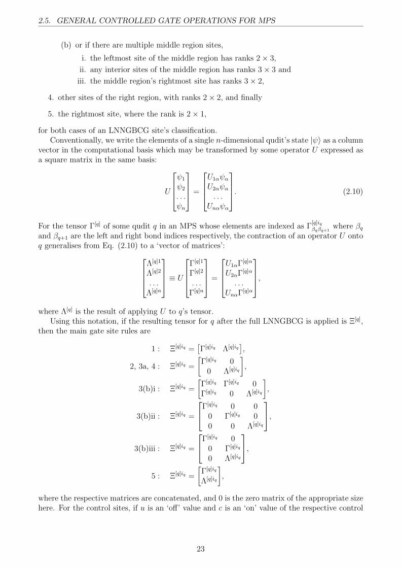
Using this notation, if the resulting tensor for q after the full LNNGBCG is applied is Ξ[q],then the main gate site rules are
1 : Ξ[q]iq =[Γ[q]iq Λ[q]iq
],
2, 3a, 4 : Ξ[q]iq =
[Γ[q]iq 0
0 Λ[q]iq
],
3(b)i : Ξ[q]iq =
[Γ[q]iq Γ[q]iq 0Γ[q]iq 0 Λ[q]iq
],
3(b)ii : Ξ[q]iq =
Γ[q]iq 0 00 Γ[q]iq 00 0 Λ[q]iq
,3(b)iii : Ξ[q]iq =
Γ[q]iq 00 Γ[q]iq
0 Λ[q]iq
,5 : Ξ[q]iq =
[Γ[q]iq
Λ[q]iq
],
where the respective matrices are concatenated, and 0 is the zero matrix of the appropriate sizehere. For the control sites, if u is an ‘off’ value and c is an ‘on’ value of the respective control
23
2.6. DENSITY MATRICES IN MPS
in the LNNGBCG, we have the rules
1 : Ξ[q]u =[Γ[q]u 0
], 1 : Ξ[q]c =
[0 Γ[q]c
],
2 : Ξ[q]u =
[Γ[q]u 0Γ[q]u 0
], 2 : Ξ[q]c =
[Γ[q]c 0
0 Γ[q]c
],
3a : Ξ[q]u =
[Γ[q]u 0
0 0
], 3a : Ξ[q]c =
[0 00 Γ[q]c
],
3(b)i : Ξ[q]u =
[Γ[q]u Γ[q]u 0
0 0 0
], 3(b)i : Ξ[q]c =
[Γ[q]c 0 0
0 0 Γ[q]c
],
3(b)ii : Ξ[q]u =
Γ[q]u Γ[q]u 00 0 00 0 0
, 3(b)ii : Ξ[q]c =
Γ[q]c 0 00 Γ[q]c 00 0 Γ[q]c
,3(b)iii : Ξ[q]u =
Γ[q]u 00 00 0
, 3(b)iii : Ξ[q]c =
0 0Γ[q]c 0
0 Γ[q]c
,4 : Ξ[q]u =
[Γ[q]u Γ[q]u
0 0
], 4 : Ξ[q]c =
[Γ[q]c 0
0 Γ[q]c
],
5 : Ξ[q]u =
[Γ[q]u
0
], 5 : Ξ[q]c =
[0
Γ[q]c
].
For bipartitions of operator Schmidt rank bounded by 2 (3), the corresponding bond vectors ofthe MPS are tiled twice (thrice).
These rules satisfy the first and second desirable traits from above: they are block sparseand only rely on values from the original qudit tensor or from the qudit tensor after applying amain gate. Furthermore, they are consistent with our assertion that the operator Schmidt rankacross any bipartition of an LNNGBCG is bounded above by 2 or 3 depending on whether ornot the bipartition has at least one main gate and one control on both sides. Though we haven’tproven opimality of this classification, we motivate it by claiming that a rank of 3 results fromcontrols on each side of a bipartition controlling main gates on the opposite side, whilst a rankof 2 results from controls on only one side of a bipartition controlling gates on the oppositeside.
Application of an LNNGBCG does not maintain canonicalisation of the MPS. The MPS canbe recanonicalised as mentioned in subsection 2.4.6 for general MPOs, where the contractionand decomposition operations of a single sweep are performed as each individual qudit andbond tensor is subsequently transformed.
2.6 Density matrices in MPS
Just as the tensor network principles allow us to decompose a state vector into an MPS, ageneral density matrix
ρ =∑i
pi |ψi〉〈ψi| (2.11)
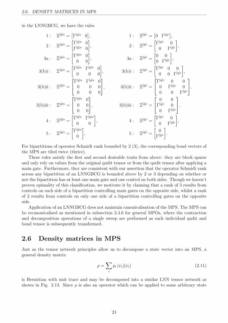
is Hermitian with unit trace and may be decomposed into a similar LNN tensor network asshown in Fig. 2.13. Since ρ is also an operator which can be applied to some arbitrary state
24
2.6. DENSITY MATRICES IN MPS
|ψ〉 as
ρ |ψ〉 =∑i
〈ψi|ψ〉 |ψi〉 ,
the tensor network decomposition of a density matrix is, infact, an MPO. However, we willspecifically refer to these as matrix product density operators (MPDOs) for density matrices.Eq. (2.11) implies a tensor product of state vectors, so if an MPDO is to follow the LNN form
of an MPS, each qudit q of the MPDO holds some tensor Θ[q] with four indices as Θ[q]iqjqαqαq+1 ,
where αq and αq+1 are the familiar left and right bond indices akin to those in an MPS and iqand jq correspond to q’s indices in the overall density matrix. The bond tensors are similarlyvectors resulting from the SVD as our decomposition.
Figure 2.13: Tensor network for an MPDO of four qudits. Cf. Fig. 2.7a.
In subsection 2.4.1, we discussed a canonical form for an MPS which allowed us to obtaina qudit’s reduced density matrix locally and hence perform single qudit measurements locally.This canonical form resulted from unitarity of the SVD and normalisation of a state, 〈ψ|ψ〉 = 1,which can also be seen if we consider the density matrix ρ of the pure state |ψ〉 also contractedwith its dual:
tr(ρρ†) = 〈ψ|ψ〉 〈ψ|ψ〉= 1.
Though we can still choose to use the SVD, no similar normalisation for a general, potentiallymixed density matrix exists, which is unsurprising given that this quantity is also referred toas a state’s purity:
tr(ρρ†) = tr(ρ2)
≤ 1
where the equality results from the density matrix being Hermitian. Therefore, a similarcanonical form for our MPDOs cannot be used to locally obtain a qudit’s reduced densitymatrix or perform a single qudit measurement. We are required to trace over all other indices(in a similar fashion to Fig. 2.7b) in order to obtain a qudit’s reduced density matrix andmeasure it. However, we may still define a canonical form for MPDOs similar to that of MPSs,the only difference being that a ‘loop’ (like in Fig. 2.9a) has an extra contracted index linecorresponding to the density matrix’s extra set of indices, and that the rightmost (leftmost)qudit will have a left (right) loop equal to tr(ρ2) instead of 1 for all other qudits. The operationsto maintain this canonical form, including sweeps, have the benefit of minimising the bondtensors’ dimensions to their respective operator Schmidt ranks at each bipartition.
A gate operation U on an MPDO now requires a contraction with U and its adjoint:
ρ←∑i
piU |ψ〉〈ψ|U † = UρU †,
25
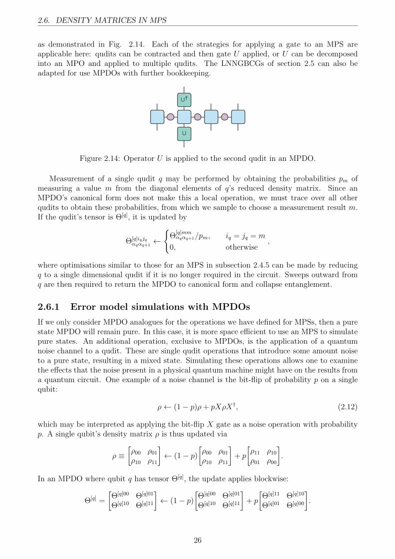
2.6. DENSITY MATRICES IN MPS
as demonstrated in Fig. 2.14. Each of the strategies for applying a gate to an MPS areapplicable here: qudits can be contracted and then gate U applied, or U can be decomposedinto an MPO and applied to multiple qudits. The LNNGBCGs of section 2.5 can also beadapted for use MPDOs with further bookkeeping.
U
U?
Figure 2.14: Operator U is applied to the second qudit in an MPDO.
Measurement of a single qudit q may be performed by obtaining the probabilities pm ofmeasuring a value m from the diagonal elements of q’s reduced density matrix. Since anMPDO’s canonical form does not make this a local operation, we must trace over all otherqudits to obtain these probabilities, from which we sample to choose a measurement result m.If the qudit’s tensor is Θ[q], it is updated by
Θ[q]iqjqαqαq+1
←
{Θ
[q]mmαqαq+1/pm, iq = jq = m
0, otherwise,
where optimisations similar to those for an MPS in subsection 2.4.5 can be made by reducingq to a single dimensional qudit if it is no longer required in the circuit. Sweeps outward fromq are then required to return the MPDO to canonical form and collapse entanglement.
2.6.1 Error model simulations with MPDOs
If we only consider MPDO analogues for the operations we have defined for MPSs, then a purestate MPDO will remain pure. In this case, it is more space efficient to use an MPS to simulatepure states. An additional operation, exclusive to MPDOs, is the application of a quantumnoise channel to a qudit. These are single qudit operations that introduce some amount noiseto a pure state, resulting in a mixed state. Simulating these operations allows one to examinethe effects that the noise present in a physical quantum machine might have on the results froma quantum circuit. One example of a noise channel is the bit-flip of probability p on a singlequbit:
ρ← (1− p)ρ+ pXρX†, (2.12)
which may be interpreted as applying the bit-flip X gate as a noise operation with probabilityp. A single qubit’s density matrix ρ is thus updated via
ρ ≡[ρ00 ρ01ρ10 ρ11
]← (1− p)
[ρ00 ρ01ρ10 ρ11
]+ p
[ρ11 ρ10ρ01 ρ00
].
In an MPDO where qubit q has tensor Θ[q], the update applies blockwise:
Θ[q] =
[Θ[q]00 Θ[q]01
Θ[q]10 Θ[q]11
]← (1− p)
[Θ[q]00 Θ[q]01
Θ[q]10 Θ[q]11
]+ p
[Θ[q]11 Θ[q]10
Θ[q]01 Θ[q]00
].
26
2.6. DENSITY MATRICES IN MPS
Applying a noise channel is a discrete operation used to model the effects of introducing aspecific kind of quantum noise to a system. When modelling noise, the choice and placementof a noise channel in a circuit must be considered. Bit-flip channels, for example, may beapplied to each qubit in a quantum circuit immediately following initialisation or precedingmeasurement to model initialisation and measurement errors respectively.
One more example of a noise channel is the depolarising channel, which updates the densitymatrix ρ of a general n-dimensional qudit as
ρ← (1− p)ρ+ p tr(ρ)Inn
(2.13)
where In is the n × n identity matrix. Here, In/n =∑n−1
i=01n|i〉〈i| is the density matrix of the
fully mixed or fully depolarised state and tr(ρ) = 1 is a convenient way to relate its elementsto ρ’s. Therefore, the depolarising channel can be interpreted as depolarising a state withprobability p, and a qubit q with tensor Θ[q] in an MPDO is updated via
Θ[q] ← (1− p)Θ[q] + p1
2
[Θ[q]00 + Θ[q]11 0
0 Θ[q]00 + Θ[q]11
],
which generalises to higher dimensions n by summing over more diagonal blocks Θ[q]iqiq . Thesedepolarising channels are often placed after the usual gate operations.
Since noise channels can be expected to decohere quantum states, entanglement in ourMPDO should accordingly collapse. Therefore, sweeps outward in both directions from the qu-dit to which a noise channel is applied are required to propagate this collapse and recanonicalisean MPDO, in a similar fashion to single qudit measurement.
Several more standard noise channels have also been defined, and can be found in [39].QCMPS includes functionality for also applying user-pecified noise channels.
2.6.2 Alternate approaches for density matrix simulations
A straightforward approach to reproducing the measurement statistics of a density matrixsimulated with noise channels is to sample from sufficiently many state vectors. For example,if a bit-flip channel of Eq. (2.12) is applied to qubit q, we could emulate it with a statevector by applying the X gate to q with probability p and averaging over the measurementprobabilities for a sufficiently large sample of such state vector runs. Since the space usage ofan MPS is significantly lower than its MPDO counterpart, we are effectively trading this spacesaving for the additional time required to sufficiently sample noise outcomes. If a significantamount of noise is introduced, enough entanglement in an MPDO may be collapsed throughcanonicalisation, and an MPS may require far too many samples to sufficiently characterisethe error model. In this case, it makes sense to use the MPDO formalism. Furthermore, toaverage over the measurement probabilities for a subsystem q of an MPS, the diagonal elementsof q’s reduced density matrix are required. The constituent qudit subsystems of q may needto be swapped and contracted to form a qudit for q to obtain this reduced density matrix. Ifthe dimensionality of q is very large, there may be space limitations in even just storing themeasurement probabilities; if q is the entire system, then a full contraction is required. However,with an MPDO, each qudit subsystem can be measured sequentially without full contraction,allowing us to sample from the correct measurement probability distribution without incurringthis memory cost.
27
2.7. COMPARISON TO EXISTING QUANTUM SIMULATORS
2.7 Comparison to existing quantum simulators
One of the simplest and most complete quantum simulator packages is the open source QuantumToolbox in Python (QuTiP) [18]. Built upon NumPy [26], it also interfaces with the rest of theSciPy stack to provide rich plotting capabilities through Matplotlib [40]. QCMPS in its currentform does not support any visualisation capabilities, but may in the future. Though QuTiPrelies on the simpler state vector and density matrix formalisms in its calculations as opposedto our MPS or MPDO methods and is limited to shared memory parallelism, it does internallystore its tensors sparsely, leading to decreased time and space usage in certain situations. Thetensors in QCMPS are stored densely, since Elemental [32] only supports dense, distributedSVD.
QCMPS was built upon Elemental in order to utilise distributed memory architecturesto overcome the space limitations of shared memory systems. One other distributed memoryquantum simulator is qHiPSTER [19], a similar simulator described by Boixo et al. in [17]. Thisis solely a state vector simulator, without any density matrix, MPS or MPDO functionality.Furthermore, it is limited to single-qubit gates and singly-controlled single-qubit gates suchas the CNot, forcing the user to decompose their circuits. In some sense, this extra stepis analogous to the extra Swap gates required to map a general gate to an MPS or MPDO.While an MPS may have a space and time advantage over a state vector when a state has lowentanglement, its space complexity is equal (O(2n) for an n qubit system) to a state vector’sfor sufficiently entangled states. In this case, a state vector simulator is advantageous timewise,since it has no need to apply expensive matrix decompositions such as the SVD that may or maynot scale well with additional CPU cores. Indeed, simple controlled or uncontrolled single qubitgates as tensor contractions to a state vector are extremely parallelisable, and qHipster makesuse of vectorisation, multithreading and cache locality optimisations to increase its performance.
Most libraries for manipulating MPSs focus not on quantum circuit simulations, but ratherdifferent algorithms such as the density matrix renormalisation group (DMRG) [22] or time-evolving block decimation (TEBD) [23] for general quantum many-body problems or problemsin quantum chemistry. Though outside the scope of this thesis, their feature requirements areslightly different to our circuit simulator: we place more emphasis on strict canonicalisation toallow local measurement of any qudit at any time, requiring use of the SVD. Two noteworthytensor network libraries are ITensor [41] and Tensor Network Theory (TNT) [42]. ITensor is apurely shared memory library, while TNT is single-node GPU-accelerated. These are general-purpose tensor network libraries that can be used to implement the operations of QCMPS onsingle node architectures.
In summary, QCMPS uniquely combines distributed memory parallelism for one-dimensionalquantum circuit simulation with original features such as LNNGBCGs and noisy MPDO func-tionality.
28
Chapter 3
Shor’s Algorithm Simulations
In order to benchmark our MPS library QCMPS, we apply a similar technique to [24] withadditional optimisations to perform a simulation of Shor’s algorithm [2] for factoring semiprimeintegers. We will present the optimisations used to factor a semiprime of 20 binary digitsthrough a simulation of a high-level quantum circuit for Shor’s algorithm requiring 60 qubits.For comparison, a state vector for 60 qubits requires us to store 260 complex scalars. Atdouble precision (64 bit real and 64 bit imaginary components), this requires a minimum storagecapacity of 16 EiB, more than the available memory of any currently existing supercomputertoday [15]. The MPS approach from [24] of simulating Shor’s algorithm is able to reduce thememory requirements by quantifying the amount of entanglement in relation to the factoredsemiprime and other parameters. However, through our optimisations, we introduce an evenmore efficient method, allowing us to simulate a 60 qubit instance of Shor’s algorithm withparameters that would be considered infeasible by the method of [24]. This stands as potentiallythe largest simulation of a non-trivial quantum circuit ever performed.
3.1 Review of Shor’s algorithm
Shor’s algorithm [2] can be used to factor a semiprime integer N = p × q of l binary digits inpolynomial time with respect to l on a quantum computer. Presently, there is no known algo-rithm to perform this factorisation efficiently (i.e. in polynomial time) on a classical computer.The presumed difficulty of factoring very large semiprime numbers is the foundation beneaththe security of the RSA public key cryptosystem [9] used to secure online communications [43],thus providing the motivation to build quantum computers capable of performing large enoughinstances of Shor’s algorithm and to develop public key cryptosystems resistant to quantumcomputers [10]. For this review, we perform the circuit shown in Fig. 3.1.
Given N , a semiprime integer represented by at least l binary digits, a high-level circuit forShor’s algorithm as detailed in [39] consists of a ‘lower’ register R of l qubits initialised to thestate |1〉 and an ‘upper’ register of 2l qubits initialised to |0〉:
|ψinit〉 ← |0〉 |1〉 .
The Hadamard gate, Eq. (2.3), is then applied to each qubit of the upper register, creating thesuperposition
|ψsuperpos〉 ← (H⊗2l)⊗ (I⊗l) |ψinit〉
=22l−1∑i=0
|i〉 |1〉 ,
29
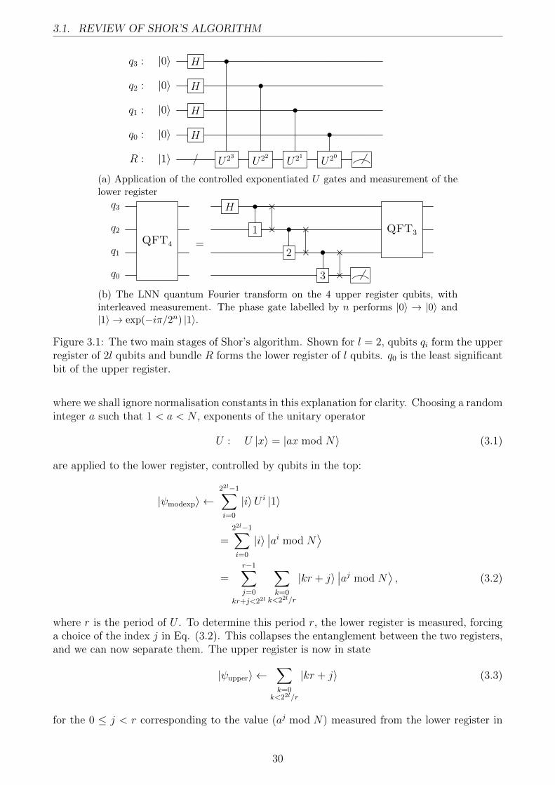
3.1. REVIEW OF SHOR’S ALGORITHM
q3 : |0〉 H •
q2 : |0〉 H •
q1 : |0〉 H •
q0 : |0〉 H •
R : |1〉 / U23 U22 U21 U20
(a) Application of the controlled exponentiated U gates and measurement of thelower register
q3
QFT4
H • ×
QFT3q2 1 × • ×
q1=
2 × • ×
q0 3 ×
(b) The LNN quantum Fourier transform on the 4 upper register qubits, withinterleaved measurement. The phase gate labelled by n performs |0〉 → |0〉 and|1〉 → exp(−iπ/2n) |1〉.
Figure 3.1: The two main stages of Shor’s algorithm. Shown for l = 2, qubits qi form the upperregister of 2l qubits and bundle R forms the lower register of l qubits. q0 is the least significantbit of the upper register.
where we shall ignore normalisation constants in this explanation for clarity. Choosing a randominteger a such that 1 < a < N , exponents of the unitary operator
U : U |x〉 = |ax mod N〉 (3.1)
are applied to the lower register, controlled by qubits in the top:
|ψmodexp〉 ←22l−1∑i=0
|i〉U i |1〉
=22l−1∑i=0
|i〉∣∣ai mod N
⟩=
r−1∑j=0
kr+j<22l
∑k=0
k<22l/r
|kr + j〉∣∣aj mod N
⟩, (3.2)
where r is the period of U . To determine this period r, the lower register is measured, forcinga choice of the index j in Eq. (3.2). This collapses the entanglement between the two registers,and we can now separate them. The upper register is now in state
|ψupper〉 ←∑k=0
k<22l/r
|kr + j〉 (3.3)
for the 0 ≤ j < r corresponding to the value (aj mod N) measured from the lower register in
30
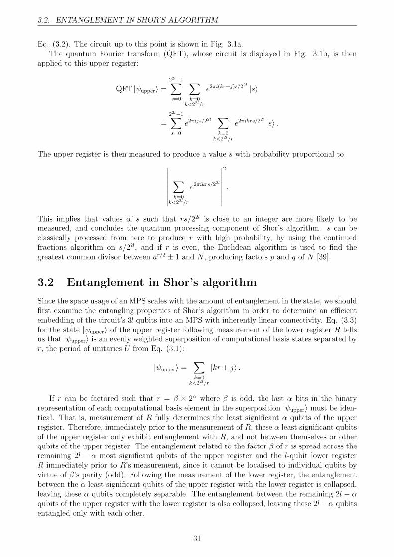
3.2. ENTANGLEMENT IN SHOR’S ALGORITHM
Eq. (3.2). The circuit up to this point is shown in Fig. 3.1a.The quantum Fourier transform (QFT), whose circuit is displayed in Fig. 3.1b, is then
applied to this upper register:
QFT |ψupper〉 =22l−1∑s=0
∑k=0
k<22l/r
e2πi(kr+j)s/22l |s〉
=22l−1∑s=0
e2πijs/22l∑k=0
k<22l/r
e2πikrs/22l |s〉 .
The upper register is then measured to produce a value s with probability proportional to∣∣∣∣∣∣∣∣∑k=0
k<22l/r
e2πikrs/22l
∣∣∣∣∣∣∣∣2
.
This implies that values of s such that rs/22l is close to an integer are more likely to bemeasured, and concludes the quantum processing component of Shor’s algorithm. s can beclassically processed from here to produce r with high probability, by using the continuedfractions algorithm on s/22l, and if r is even, the Euclidean algorithm is used to find thegreatest common divisor between ar/2 ± 1 and N , producing factors p and q of N [39].
3.2 Entanglement in Shor’s algorithm
Since the space usage of an MPS scales with the amount of entanglement in the state, we shouldfirst examine the entangling properties of Shor’s algorithm in order to determine an efficientembedding of the circuit’s 3l qubits into an MPS with inherently linear connectivity. Eq. (3.3)for the state |ψupper〉 of the upper register following measurement of the lower register R tellsus that |ψupper〉 is an evenly weighted superposition of computational basis states separated byr, the period of unitaries U from Eq. (3.1):
|ψupper〉 =∑k=0
k<22l/r
|kr + j〉 .
If r can be factored such that r = β × 2α where β is odd, the last α bits in the binaryrepresentation of each computational basis element in the superposition |ψupper〉 must be iden-tical. That is, measurement of R fully determines the least significant α qubits of the upperregister. Therefore, immediately prior to the measurement of R, these α least significant qubitsof the upper register only exhibit entanglement with R, and not between themselves or otherqubits of the upper register. The entanglement related to the factor β of r is spread across theremaining 2l − α most significant qubits of the upper register and the l-qubit lower registerR immediately prior to R’s measurement, since it cannot be localised to individual qubits byvirtue of β’s parity (odd). Following the measurement of the lower register, the entanglementbetween the α least significant qubits of the upper register with the lower register is collapsed,leaving these α qubits completely separable. The entanglement between the remaining 2l − αqubits of the upper register with the lower register is also collapsed, leaving these 2l−α qubitsentangled only with each other.
31
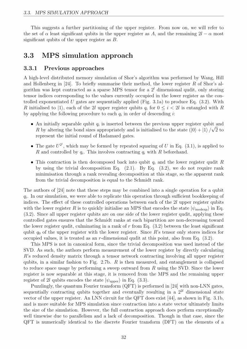
3.3. MPS SIMULATION APPROACH
This suggests a further partitioning of the upper register. From now on, we will refer tothe set of α least significant qubits in the upper register as A, and the remaining 2l − α mostsignificant qubits of the upper register as B.
3.3 MPS simulation approach
3.3.1 Previous approaches
A high-level distributed memory simulation of Shor’s algorithm was performed by Wang, Hilland Hollenberg in [24]. To briefly summarise their method, the lower register R of Shor’s al-gorithm was kept contracted as a sparse MPS tensor for a 2l dimensional qudit, only storingtensor indices corresponding to the values currently occupied in the lower register as the con-trolled exponentiated U gates are sequentially applied (Fig. 3.1a) to produce Eq. (3.2). WithR initialised to |1〉, each of the 2l upper register qubits qi for 0 ≤ i < 2l is entangled with Rby applying the following procedure to each qi in order of descending i:
• An initially separable qubit qi is inserted between the previous upper register qubit andR by altering the bond sizes appropriately and is initialised to the state (|0〉+ |1〉 /
√2 to
represent the initial round of Hadamard gates.
• The gate U2i , which may be formed by repeated squaring of U in Eq. (3.1), is applied toR and controlled by qi. This involves contracting qi with R beforehand.
• This contraction is then decomposed back into qubit qi and the lower register qudit Rby using the trivial decomposition Eq. (2.1). By Eq. (3.2), we do not require rankminimisation through a rank revealing decomposition at this stage, so the apparent rankfrom the trivial decomposition is equal to the Schmidt rank.
The authors of [24] note that these steps may be combined into a single operation for a qubitqi. In our simulation, we were able to replicate this operation through sufficient bookkeeping ofindices. The effect of these controlled operations between each of the 2l upper register qubitswith the lower register R is to quickly initialise an MPS that encodes the state |ψmodexp〉 in Eq.(3.2). Since all upper register qubits are on one side of the lower register qudit, applying thesecontrolled gates ensures that the Schmidt ranks at each bipartition are non-decreasing towardthe lower register qudit, culminating in a rank of r from Eq. (3.2) between the least significantqubit q0 of the upper register with the lower register. Since R’s tensor only stores indices foroccupied values, it is treated as an r-dimensional qudit at this point, also from Eq. (3.2).
This MPS is not in canonical form, since the trivial decomposition was used instead of theSVD. As such, the authors perform measurement of the lower register by directly calculatingR’s reduced density matrix through a tensor network contracting involving all upper registerqubits, in a similar fashion to Fig. 2.7b. R is then measured, and entanglement is collapsedto reduce space usage by performing a sweep outward from R using the SVD. Since the lowerregister is now separable at this stage, it is removed from the MPS and the remaining upperregister of 2l qubits encodes the state |ψupper〉 in Eq. (3.3).
Puzzlingly, the quantum Fourier transform (QFT) is performed in [24] with non-LNN gates,sequentially contracting qubits together and eventually resulting in a 22l dimensional statevector of the upper register. An LNN circuit for the QFT does exist [44], as shown in Fig. 3.1b,and is more suitable for MPS simulation since contraction into a state vector ultimately limitsthe size of the simulation. However, the full contraction approach does perform exceptionallywell timewise due to parallelism and a lack of decomposition. Though in that case, since theQFT is numerically identical to the discrete Fourier transform (DFT) on the elements of a
32
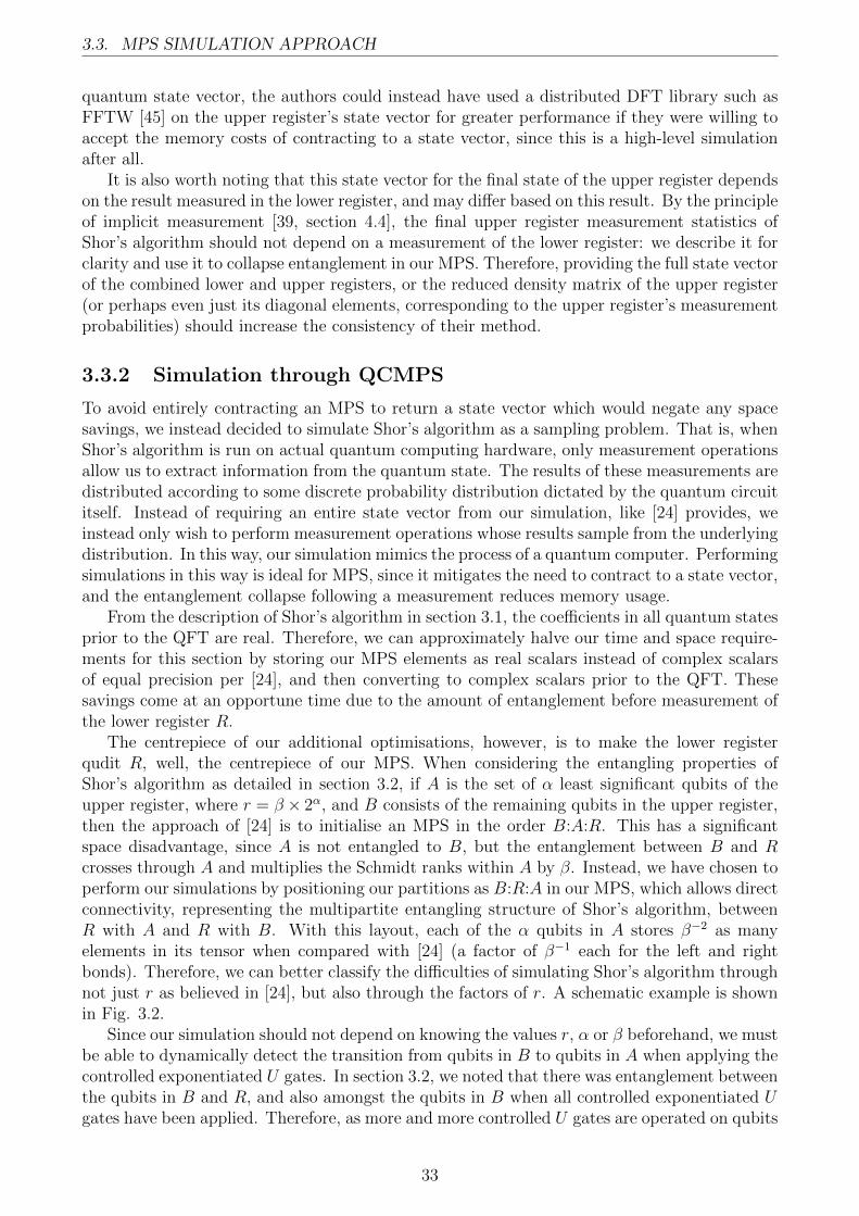
3.3. MPS SIMULATION APPROACH
quantum state vector, the authors could instead have used a distributed DFT library such asFFTW [45] on the upper register’s state vector for greater performance if they were willing toaccept the memory costs of contracting to a state vector, since this is a high-level simulationafter all.
It is also worth noting that this state vector for the final state of the upper register dependson the result measured in the lower register, and may differ based on this result. By the principleof implicit measurement [39, section 4.4], the final upper register measurement statistics ofShor’s algorithm should not depend on a measurement of the lower register: we describe it forclarity and use it to collapse entanglement in our MPS. Therefore, providing the full state vectorof the combined lower and upper registers, or the reduced density matrix of the upper register(or perhaps even just its diagonal elements, corresponding to the upper register’s measurementprobabilities) should increase the consistency of their method.
3.3.2 Simulation through QCMPS
To avoid entirely contracting an MPS to return a state vector which would negate any spacesavings, we instead decided to simulate Shor’s algorithm as a sampling problem. That is, whenShor’s algorithm is run on actual quantum computing hardware, only measurement operationsallow us to extract information from the quantum state. The results of these measurements aredistributed according to some discrete probability distribution dictated by the quantum circuititself. Instead of requiring an entire state vector from our simulation, like [24] provides, weinstead only wish to perform measurement operations whose results sample from the underlyingdistribution. In this way, our simulation mimics the process of a quantum computer. Performingsimulations in this way is ideal for MPS, since it mitigates the need to contract to a state vector,and the entanglement collapse following a measurement reduces memory usage.
From the description of Shor’s algorithm in section 3.1, the coefficients in all quantum statesprior to the QFT are real. Therefore, we can approximately halve our time and space require-ments for this section by storing our MPS elements as real scalars instead of complex scalarsof equal precision per [24], and then converting to complex scalars prior to the QFT. Thesesavings come at an opportune time due to the amount of entanglement before measurement ofthe lower register R.
The centrepiece of our additional optimisations, however, is to make the lower registerqudit R, well, the centrepiece of our MPS. When considering the entangling properties ofShor’s algorithm as detailed in section 3.2, if A is the set of α least significant qubits of theupper register, where r = β × 2α, and B consists of the remaining qubits in the upper register,then the approach of [24] is to initialise an MPS in the order B:A:R. This has a significantspace disadvantage, since A is not entangled to B, but the entanglement between B and Rcrosses through A and multiplies the Schmidt ranks within A by β. Instead, we have chosen toperform our simulations by positioning our partitions as B:R:A in our MPS, which allows directconnectivity, representing the multipartite entangling structure of Shor’s algorithm, betweenR with A and R with B. With this layout, each of the α qubits in A stores β−2 as manyelements in its tensor when compared with [24] (a factor of β−1 each for the left and rightbonds). Therefore, we can better classify the difficulties of simulating Shor’s algorithm throughnot just r as believed in [24], but also through the factors of r. A schematic example is shownin Fig. 3.2.
Since our simulation should not depend on knowing the values r, α or β beforehand, we mustbe able to dynamically detect the transition from qubits in B to qubits in A when applying thecontrolled exponentiated U gates. In section 3.2, we noted that there was entanglement betweenthe qubits in B and R, and also amongst the qubits in B when all controlled exponentiated Ugates have been applied. Therefore, as more and more controlled U gates are operated on qubits
33
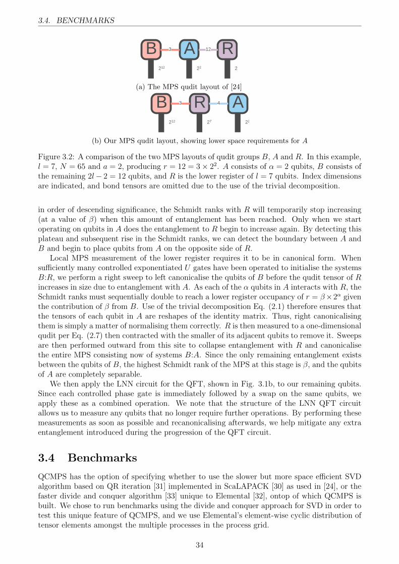
3.4. BENCHMARKS
R27
A22
B212
3 12
(a) The MPS qudit layout of [24]
R27
A22
B212
3 4
(b) Our MPS qudit layout, showing lower space requirements for A
Figure 3.2: A comparison of the two MPS layouts of qudit groups B, A and R. In this example,l = 7, N = 65 and a = 2, producing r = 12 = 3× 22. A consists of α = 2 qubits, B consists ofthe remaining 2l− 2 = 12 qubits, and R is the lower register of l = 7 qubits. Index dimensionsare indicated, and bond tensors are omitted due to the use of the trivial decomposition.
in order of descending significance, the Schmidt ranks with R will temporarily stop increasing(at a value of β) when this amount of entanglement has been reached. Only when we startoperating on qubits in A does the entanglement to R begin to increase again. By detecting thisplateau and subsequent rise in the Schmidt ranks, we can detect the boundary between A andB and begin to place qubits from A on the opposite side of R.
Local MPS measurement of the lower register requires it to be in canonical form. Whensufficiently many controlled exponentiated U gates have been operated to initialise the systemsB:R, we perform a right sweep to left canonicalise the qubits of B before the qudit tensor of Rincreases in size due to entanglement with A. As each of the α qubits in A interacts with R, theSchmidt ranks must sequentially double to reach a lower register occupancy of r = β×2α giventhe contribution of β from B. Use of the trivial decomposition Eq. (2.1) therefore ensures thatthe tensors of each qubit in A are reshapes of the identity matrix. Thus, right canonicalisingthem is simply a matter of normalising them correctly. R is then measured to a one-dimensionalqudit per Eq. (2.7) then contracted with the smaller of its adjacent qubits to remove it. Sweepsare then performed outward from this site to collapse entanglement with R and canonicalisethe entire MPS consisting now of systems B:A. Since the only remaining entanglement existsbetween the qubits of B, the highest Schmidt rank of the MPS at this stage is β, and the qubitsof A are completely separable.
We then apply the LNN circuit for the QFT, shown in Fig. 3.1b, to our remaining qubits.Since each controlled phase gate is immediately followed by a swap on the same qubits, weapply these as a combined operation. We note that the structure of the LNN QFT circuitallows us to measure any qubits that no longer require further operations. By performing thesemeasurements as soon as possible and recanonicalising afterwards, we help mitigate any extraentanglement introduced during the progression of the QFT circuit.
3.4 Benchmarks
QCMPS has the option of specifying whether to use the slower but more space efficient SVDalgorithm based on QR iteration [31] implemented in ScaLAPACK [30] as used in [24], or thefaster divide and conquer algorithm [33] unique to Elemental [32], ontop of which QCMPS isbuilt. We chose to run benchmarks using the divide and conquer approach for SVD in order totest this unique feature of QCMPS, and we use Elemental’s element-wise cyclic distribution oftensor elements amongst the multiple processes in the process grid.
34
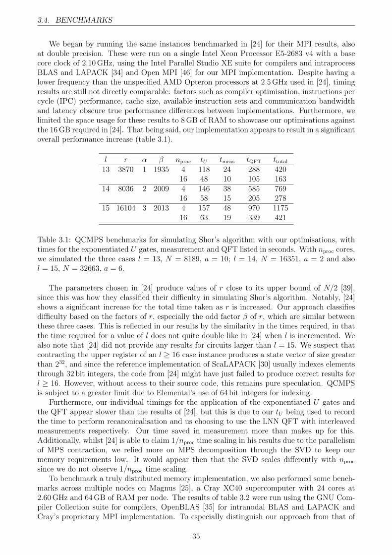
3.4. BENCHMARKS
We began by running the same instances benchmarked in [24] for their MPI results, alsoat double precision. These were run on a single Intel Xeon Processor E5-2683 v4 with a basecore clock of 2.10 GHz, using the Intel Parallel Studio XE suite for compilers and intraprocessBLAS and LAPACK [34] and Open MPI [46] for our MPI implementation. Despite having alower frequency than the unspecified AMD Opteron processors at 2.5 GHz used in [24], timingresults are still not directly comparable: factors such as compiler optimisation, instructions percycle (IPC) performance, cache size, available instruction sets and communication bandwidthand latency obscure true performance differences between implementations. Furthermore, welimited the space usage for these results to 8 GB of RAM to showcase our optimisations againstthe 16 GB required in [24]. That being said, our implementation appears to result in a significantoverall performance increase (table 3.1).
l r α β nproc tU tmeas tQFT ttotal13 3870 1 1935 4 118 24 288 420
16 48 10 105 16314 8036 2 2009 4 146 38 585 769
16 58 15 205 27815 16104 3 2013 4 157 48 970 1175
16 63 19 339 421
Table 3.1: QCMPS benchmarks for simulating Shor’s algorithm with our optimisations, withtimes for the exponentiated U gates, measurement and QFT listed in seconds. With nproc cores,we simulated the three cases l = 13, N = 8189, a = 10; l = 14, N = 16351, a = 2 and alsol = 15, N = 32663, a = 6.
The parameters chosen in [24] produce values of r close to its upper bound of N/2 [39],since this was how they classified their difficulty in simulating Shor’s algorithm. Notably, [24]shows a significant increase for the total time taken as r is increased. Our approach classifiesdifficulty based on the factors of r, especially the odd factor β of r, which are similar betweenthese three cases. This is reflected in our results by the similarity in the times required, in thatthe time required for a value of l does not quite double like in [24] when l is incremented. Wealso note that [24] did not provide any results for circuits larger than l = 15. We suspect thatcontracting the upper register of an l ≥ 16 case instance produces a state vector of size greaterthan 232, and since the reference implementation of ScaLAPACK [30] usually indexes elementsthrough 32 bit integers, the code from [24] might have just failed to produce correct results forl ≥ 16. However, without access to their source code, this remains pure speculation. QCMPSis subject to a greater limit due to Elemental’s use of 64 bit integers for indexing.
Furthermore, our individual timings for the application of the exponentiated U gates andthe QFT appear slower than the results of [24], but this is due to our tU being used to recordthe time to perform recanonicalisation and us choosing to use the LNN QFT with interleavedmeasurements respectively. Our time saved in measurement more than makes up for this.Additionally, whilst [24] is able to claim 1/nproc time scaling in his results due to the parallelismof MPS contraction, we relied more on MPS decomposition through the SVD to keep ourmemory requirements low. It would appear then that the SVD scales differently with nproc
since we do not observe 1/nproc time scaling.To benchmark a truly distributed memory implementation, we also performed some bench-
marks across multiple nodes on Magnus [25], a Cray XC40 supercomputer with 24 cores at2.60 GHz and 64 GB of RAM per node. The results of table 3.2 were run using the GNU Com-piler Collection suite for compilers, OpenBLAS [35] for intranodal BLAS and LAPACK andCray’s proprietary MPI implementation. To especially distinguish our approach from that of
35
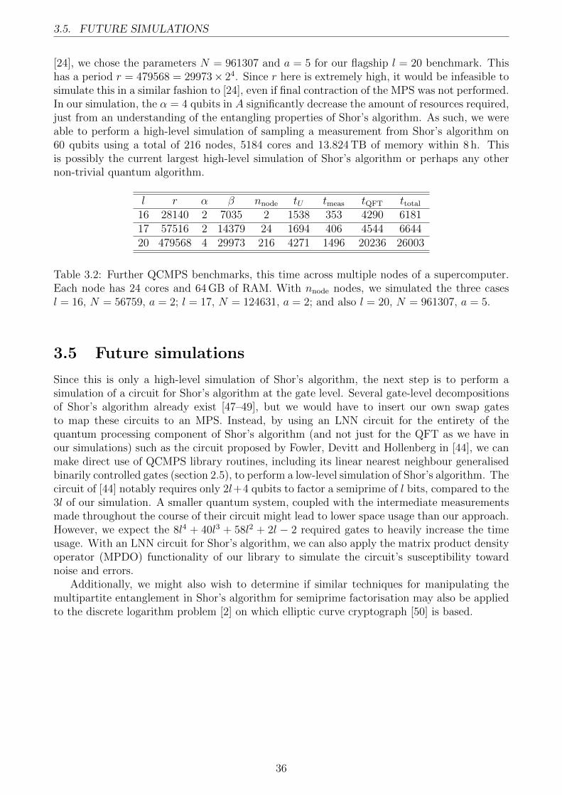
3.5. FUTURE SIMULATIONS
[24], we chose the parameters N = 961307 and a = 5 for our flagship l = 20 benchmark. Thishas a period r = 479568 = 29973× 24. Since r here is extremely high, it would be infeasible tosimulate this in a similar fashion to [24], even if final contraction of the MPS was not performed.In our simulation, the α = 4 qubits in A significantly decrease the amount of resources required,just from an understanding of the entangling properties of Shor’s algorithm. As such, we wereable to perform a high-level simulation of sampling a measurement from Shor’s algorithm on60 qubits using a total of 216 nodes, 5184 cores and 13.824 TB of memory within 8 h. Thisis possibly the current largest high-level simulation of Shor’s algorithm or perhaps any othernon-trivial quantum algorithm.
l r α β nnode tU tmeas tQFT ttotal16 28140 2 7035 2 1538 353 4290 618117 57516 2 14379 24 1694 406 4544 664420 479568 4 29973 216 4271 1496 20236 26003
Table 3.2: Further QCMPS benchmarks, this time across multiple nodes of a supercomputer.Each node has 24 cores and 64 GB of RAM. With nnode nodes, we simulated the three casesl = 16, N = 56759, a = 2; l = 17, N = 124631, a = 2; and also l = 20, N = 961307, a = 5.
3.5 Future simulations
Since this is only a high-level simulation of Shor’s algorithm, the next step is to perform asimulation of a circuit for Shor’s algorithm at the gate level. Several gate-level decompositionsof Shor’s algorithm already exist [47–49], but we would have to insert our own swap gatesto map these circuits to an MPS. Instead, by using an LNN circuit for the entirety of thequantum processing component of Shor’s algorithm (and not just for the QFT as we have inour simulations) such as the circuit proposed by Fowler, Devitt and Hollenberg in [44], we canmake direct use of QCMPS library routines, including its linear nearest neighbour generalisedbinarily controlled gates (section 2.5), to perform a low-level simulation of Shor’s algorithm. Thecircuit of [44] notably requires only 2l+4 qubits to factor a semiprime of l bits, compared to the3l of our simulation. A smaller quantum system, coupled with the intermediate measurementsmade throughout the course of their circuit might lead to lower space usage than our approach.However, we expect the 8l4 + 40l3 + 58l2 + 2l − 2 required gates to heavily increase the timeusage. With an LNN circuit for Shor’s algorithm, we can also apply the matrix product densityoperator (MPDO) functionality of our library to simulate the circuit’s susceptibility towardnoise and errors.
Additionally, we might also wish to determine if similar techniques for manipulating themultipartite entanglement in Shor’s algorithm for semiprime factorisation may also be appliedto the discrete logarithm problem [2] on which elliptic curve cryptograph [50] is based.
36
Chapter 4
Google Supremacy Circuit Simulations
In the last chapter, we investigated MPS methods for simulating Shor’s algorithm [2]. Thisalgorithm allows a quantum computer to factor a semiprime integer in polynomial time withrespect to its length in digits, a feat not demonstrated on a classical computer. Algorithmsthat show an apparent advantage of quantum computation over classical computation alludeto an inherent ‘quantum supremacy’ over classical models of computation (of which the Turingmachine [1] is one).
This notion of quantum supremacy has lead to the development of problems to specificallypinpoint instance sizes efficiently solvable on an ideal quantum computer but infeasible onany reasonable amount of classical computational hardware. There are several theoretical andexperimental challenges in demonstrating quantum supremacy, however. Open questions incomputer science regarding complexity theory (of which P versus NP [51] is a famous instance)currently prevent us from making concrete claims of any theoretical quantum supremacy: forexample, if an efficient classical algorithm for integer factorisation did exist, then performing asufficiently large instance of Shor’s algorithm on a quantum computer would not demonstratesupremacy. Implementing quantum hardware resistant enough from decoherence and noiseeffects to perform large enough instances to demonstrate supremacy is also experimentallychallenging.
Further examples [13] of problems for demonstrating quantum supremacy include bosonsampling [52], where the aim is to accurately sample the outputs of a linear optics networkwith single photon inputs. Through combinatorial arguments [14], the supremacy point of alinear optics quantum computer is expected to be around 50 single photon inputs for bosonsampling.
In this chapter, we examine the problem of sampling from random quantum circuits witha structure proposed by Google’s Boixo and Isakov et al. in [17]. Henceforth, we shall referto this problem as the Google supremacy problem. Specifically, we wish to determine if MPStechniques can be applied for classical simulation of similar circuits to refine this problem’ssupremacy point.
4.1 Introduction to the Google supremacy problem
Google’s supremacy problem [17] involves sampling measurements from the results of specificrandomly generated circuits on a two-dimensional nearest-neighbour architecture. If a randomcircuit U operates |ψ〉 ← U |ψ〉 on an n qubit system (or equivalently, a single N ≡ 2n levelsystem), the problem for either a classical computer or experimental implementation of a quan-tum computer is to sample bit strings x ∈ {0, 1}n in, say, the computational basis according tothe probability distribution resulting from applying U .
The random two-dimensional circuits are generated according to a basic structure defined
37
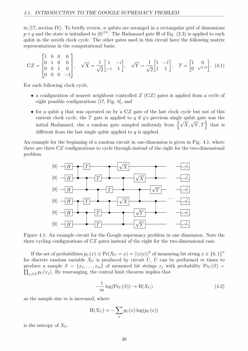
4.1. INTRODUCTION TO THE GOOGLE SUPREMACY PROBLEM
in [17, section IV]. To briefly review, n qubits are arranged in a rectangular grid of dimensionsp× q and the state is initialised to |0〉⊗n. The Hadamard gate H of Eq. (2.3) is applied to eachqubit in the zeroth clock cycle. The other gates used in this circuit have the following matrixrepresentations in the computational basis:
CZ =
1 0 0 00 1 0 00 0 1 00 0 0 −1
, √X =
1√2
[1 −i−i 1
],√Y =
1√2
[1 −11 1
], T =
[1 00 eiπ/4
]. (4.1)
For each following clock cycle,
• a configuration of nearest neighbour controlled Z (CZ) gates is applied from a cycle ofeight possible configurations [17, Fig. 6], and
• for a qubit q that was operated on by a CZ gate of the last clock cycle but not of thiscurrent clock cycle, the T gate is applied to q if q’s previous single qubit gate was the
initial Hadamard, else a random gate sampled uniformly from{√
X,√Y , T
}that is
different from the last single qubit applied to q is applied.
An example for the beginning of a random circuit in one-dimension is given in Fig. 4.1, wherethere are three CZ configurations to cycle through instead of the eight for the two-dimensionalproblem.
|0〉 H • T •√X •
|0〉 H • • T • •√X •
|0〉 H • • T • •√Y
|0〉 H • T • •√X • •
. . .
|0〉 H • • T • •√Y •
|0〉 H • T •√Y
Figure 4.1: An example circuit for the Google supremacy problem in one dimension. Note thethree cycling configurations of CZ gates instead of the eight for the two-dimensional case.
If the set of probabilities pU(x) ≡ Pr(XU = x) = |〈x|ψ〉|2 of measuring bit string x ∈ {0, 1}nfor discrete random variable XU is produced by circuit U , U can be performed m times toproduce a sample S = {x1, . . . , xm} of measured bit strings xj with probability PrU(S) =∏
xj∈S pU(xj). By rearranging, the central limit theorem implies that
− 1
mlog(PrU(S))→ H(XU) (4.2)
as the sample size m is increased, where
H(XU) = −∑x
pU(x) log(pU(x))
is the entropy of XU .
38
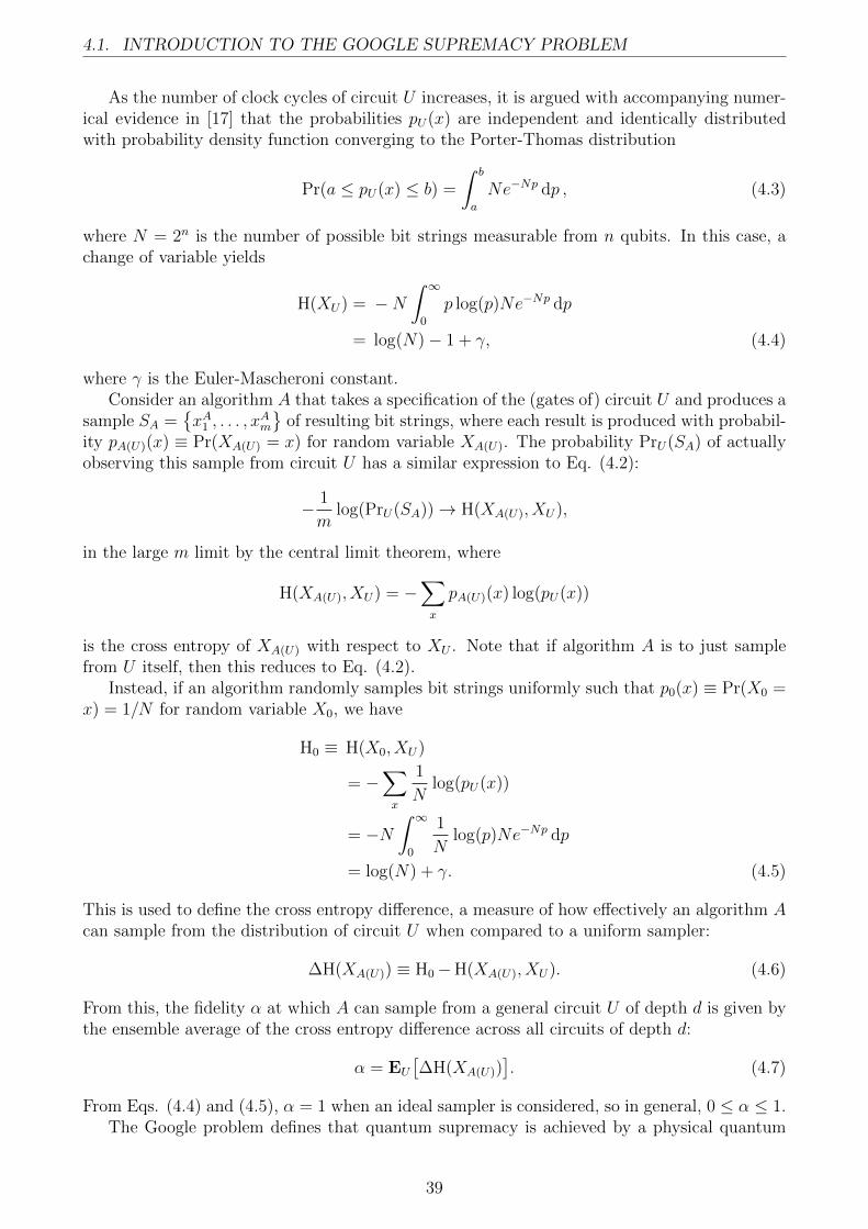
4.1. INTRODUCTION TO THE GOOGLE SUPREMACY PROBLEM
As the number of clock cycles of circuit U increases, it is argued with accompanying numer-ical evidence in [17] that the probabilities pU(x) are independent and identically distributedwith probability density function converging to the Porter-Thomas distribution
Pr(a ≤ pU(x) ≤ b) =
∫ b
a
Ne−Np dp , (4.3)
where N = 2n is the number of possible bit strings measurable from n qubits. In this case, achange of variable yields
H(XU) = −N∫ ∞0
p log(p)Ne−Np dp
= log(N)− 1 + γ, (4.4)
where γ is the Euler-Mascheroni constant.Consider an algorithm A that takes a specification of the (gates of) circuit U and produces a
sample SA ={xA1 , . . . , x
Am
}of resulting bit strings, where each result is produced with probabil-
ity pA(U)(x) ≡ Pr(XA(U) = x) for random variable XA(U). The probability PrU(SA) of actuallyobserving this sample from circuit U has a similar expression to Eq. (4.2):
− 1
mlog(PrU(SA))→ H(XA(U), XU),
in the large m limit by the central limit theorem, where
H(XA(U), XU) = −∑x
pA(U)(x) log(pU(x))
is the cross entropy of XA(U) with respect to XU . Note that if algorithm A is to just samplefrom U itself, then this reduces to Eq. (4.2).
Instead, if an algorithm randomly samples bit strings uniformly such that p0(x) ≡ Pr(X0 =x) = 1/N for random variable X0, we have
H0 ≡ H(X0, XU)
= −∑x
1
Nlog(pU(x))
= −N∫ ∞0
1
Nlog(p)Ne−Np dp
= log(N) + γ. (4.5)
This is used to define the cross entropy difference, a measure of how effectively an algorithm Acan sample from the distribution of circuit U when compared to a uniform sampler:
∆H(XA(U)) ≡ H0−H(XA(U), XU). (4.6)
From this, the fidelity α at which A can sample from a general circuit U of depth d is given bythe ensemble average of the cross entropy difference across all circuits of depth d:
α = EU
[∆H(XA(U))
]. (4.7)
From Eqs. (4.4) and (4.5), α = 1 when an ideal sampler is considered, so in general, 0 ≤ α ≤ 1.The Google problem defines that quantum supremacy is achieved by a physical quantum
39
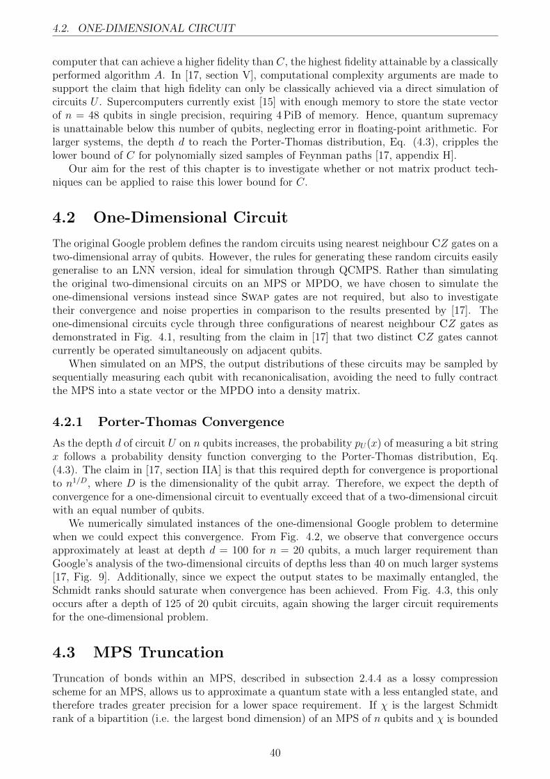
4.2. ONE-DIMENSIONAL CIRCUIT
computer that can achieve a higher fidelity than C, the highest fidelity attainable by a classicallyperformed algorithm A. In [17, section V], computational complexity arguments are made tosupport the claim that high fidelity can only be classically achieved via a direct simulation ofcircuits U . Supercomputers currently exist [15] with enough memory to store the state vectorof n = 48 qubits in single precision, requiring 4 PiB of memory. Hence, quantum supremacyis unattainable below this number of qubits, neglecting error in floating-point arithmetic. Forlarger systems, the depth d to reach the Porter-Thomas distribution, Eq. (4.3), cripples thelower bound of C for polynomially sized samples of Feynman paths [17, appendix H].
Our aim for the rest of this chapter is to investigate whether or not matrix product tech-niques can be applied to raise this lower bound for C.
4.2 One-Dimensional Circuit
The original Google problem defines the random circuits using nearest neighbour CZ gates on atwo-dimensional array of qubits. However, the rules for generating these random circuits easilygeneralise to an LNN version, ideal for simulation through QCMPS. Rather than simulatingthe original two-dimensional circuits on an MPS or MPDO, we have chosen to simulate theone-dimensional versions instead since Swap gates are not required, but also to investigatetheir convergence and noise properties in comparison to the results presented by [17]. Theone-dimensional circuits cycle through three configurations of nearest neighbour CZ gates asdemonstrated in Fig. 4.1, resulting from the claim in [17] that two distinct CZ gates cannotcurrently be operated simultaneously on adjacent qubits.
When simulated on an MPS, the output distributions of these circuits may be sampled bysequentially measuring each qubit with recanonicalisation, avoiding the need to fully contractthe MPS into a state vector or the MPDO into a density matrix.
4.2.1 Porter-Thomas Convergence
As the depth d of circuit U on n qubits increases, the probability pU(x) of measuring a bit stringx follows a probability density function converging to the Porter-Thomas distribution, Eq.(4.3). The claim in [17, section IIA] is that this required depth for convergence is proportionalto n1/D, where D is the dimensionality of the qubit array. Therefore, we expect the depth ofconvergence for a one-dimensional circuit to eventually exceed that of a two-dimensional circuitwith an equal number of qubits.
We numerically simulated instances of the one-dimensional Google problem to determinewhen we could expect this convergence. From Fig. 4.2, we observe that convergence occursapproximately at least at depth d = 100 for n = 20 qubits, a much larger requirement thanGoogle’s analysis of the two-dimensional circuits of depths less than 40 on much larger systems[17, Fig. 9]. Additionally, since we expect the output states to be maximally entangled, theSchmidt ranks should saturate when convergence has been achieved. From Fig. 4.3, this onlyoccurs after a depth of 125 of 20 qubit circuits, again showing the larger circuit requirementsfor the one-dimensional problem.
4.3 MPS Truncation
Truncation of bonds within an MPS, described in subsection 2.4.4 as a lossy compressionscheme for an MPS, allows us to approximate a quantum state with a less entangled state, andtherefore trades greater precision for a lower space requirement. If χ is the largest Schmidtrank of a bipartition (i.e. the largest bond dimension) of an MPS of n qubits and χ is bounded
40
4.3. MPS TRUNCATION
0 25 50 75 100 125 150 175 200
Depth
6
8
10
12
14Entropy
n = 10
n = 12
n = 14
n = 16
n = 18
n = 20
Figure 4.2: Mean output distribution entropies as a function of circuit depth. Sampled over100 random circuits each, the error bars represent one standard deviation. The black dashedlines are the respective Porter-Thomas entropies for the number of qubits n.
0 25 50 75 100 125 150 175 200
Depth
22
24
26
28
210
GreatestSchmidtRank
n = 10
n = 12
n = 14
n = 16
n = 18
n = 20
Figure 4.3: Mean maximum Schmidt ranks in the MPS as a function of depth. Sampled over100 instances, the shading represents one standard deviation.
41
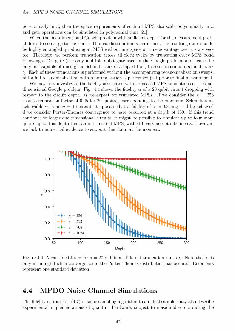
4.4. MPDO NOISE CHANNEL SIMULATIONS
polynomially in n, then the space requirements of such an MPS also scale polynomially in nand gate operations can be simulated in polynomial time [21].
When the one-dimensional Google problem with sufficient depth for the measurement prob-abilities to converge to the Porter-Thomas distribution is performed, the resulting state shouldbe highly entangled, producing an MPS without any space or time advantage over a state vec-tor. Therefore, we perform truncation across all clock cycles by truncating every MPS bondfollowing a CZ gate (the only multiple qubit gate used in the Google problem and hence theonly one capable of raising the Schmidt rank of a bipartition) to some maximum Schmidt rankχ. Each of these truncations is performed without the accompanying recanonicalisation sweeps,but a full recanonicalisation with renormalisation is performed just prior to final measurement.
We may now investigate the fidelity associated with truncated MPS simulations of the one-dimensional Google problem. Fig. 4.4 shows the fidelity α of a 20 qubit circuit dropping withrespect to the circuit depth, as we expect for truncated MPSs. If we consider the χ = 256case (a truncation factor of 0.25 for 20 qubits), corresponding to the maximum Schmidt rankachievable with an n = 16 circuit, it appears that a fidelity of α ≈ 0.3 may still be achievedif we consider Porter-Thomas convergence to have occurred at a depth of 150. If this trendcontinues to larger one-dimensional circuits, it might be possible to simulate up to four morequbits up to this depth than an untruncated MPS, with still very acceptable fidelity. However,we lack to numerical evidence to support this claim at the moment.
50 100 150 200 250 300
Depth
0.0
0.2
0.4
0.6
0.8
1.0
α
χ = 256
χ = 512
χ = 768
χ = 1024
Figure 4.4: Mean fidelities α for n = 20 qubits at different truncation ranks χ. Note that α isonly meaningful when convergence to the Porter-Thomas distribution has occured. Error barsrepresent one standard deviation.
4.4 MPDO Noise Channel Simulations
The fidelity α from Eq. (4.7) of some sampling algorithm to an ideal sampler may also describeexperimental implementations of quantum hardware, subject to noise and errors during the
42
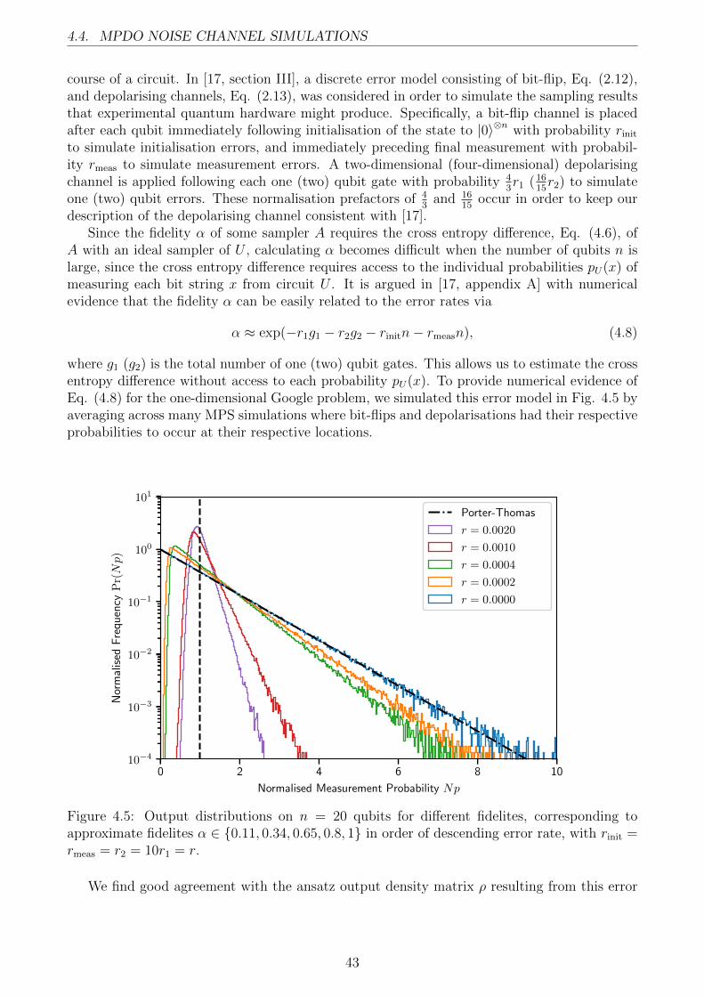
4.4. MPDO NOISE CHANNEL SIMULATIONS
course of a circuit. In [17, section III], a discrete error model consisting of bit-flip, Eq. (2.12),and depolarising channels, Eq. (2.13), was considered in order to simulate the sampling resultsthat experimental quantum hardware might produce. Specifically, a bit-flip channel is placedafter each qubit immediately following initialisation of the state to |0〉⊗n with probability rinitto simulate initialisation errors, and immediately preceding final measurement with probabil-ity rmeas to simulate measurement errors. A two-dimensional (four-dimensional) depolarisingchannel is applied following each one (two) qubit gate with probability 4
3r1 (16
15r2) to simulate
one (two) qubit errors. These normalisation prefactors of 43
and 1615
occur in order to keep ourdescription of the depolarising channel consistent with [17].
Since the fidelity α of some sampler A requires the cross entropy difference, Eq. (4.6), ofA with an ideal sampler of U , calculating α becomes difficult when the number of qubits n islarge, since the cross entropy difference requires access to the individual probabilities pU(x) ofmeasuring each bit string x from circuit U . It is argued in [17, appendix A] with numericalevidence that the fidelity α can be easily related to the error rates via
α ≈ exp(−r1g1 − r2g2 − rinitn− rmeasn), (4.8)
where g1 (g2) is the total number of one (two) qubit gates. This allows us to estimate the crossentropy difference without access to each probability pU(x). To provide numerical evidence ofEq. (4.8) for the one-dimensional Google problem, we simulated this error model in Fig. 4.5 byaveraging across many MPS simulations where bit-flips and depolarisations had their respectiveprobabilities to occur at their respective locations.
0 2 4 6 8 10
Normalised Measurement Probability Np
10−4
10−3
10−2
10−1
100
101
Normalised
Frequency
Pr(Np)
Porter-Thomas
r = 0.0020
r = 0.0010
r = 0.0004
r = 0.0002
r = 0.0000
Figure 4.5: Output distributions on n = 20 qubits for different fidelites, corresponding toapproximate fidelites α ∈ {0.11, 0.34, 0.65, 0.8, 1} in order of descending error rate, with rinit =rmeas = r2 = 10r1 = r.
We find good agreement with the ansatz output density matrix ρ resulting from this error
43
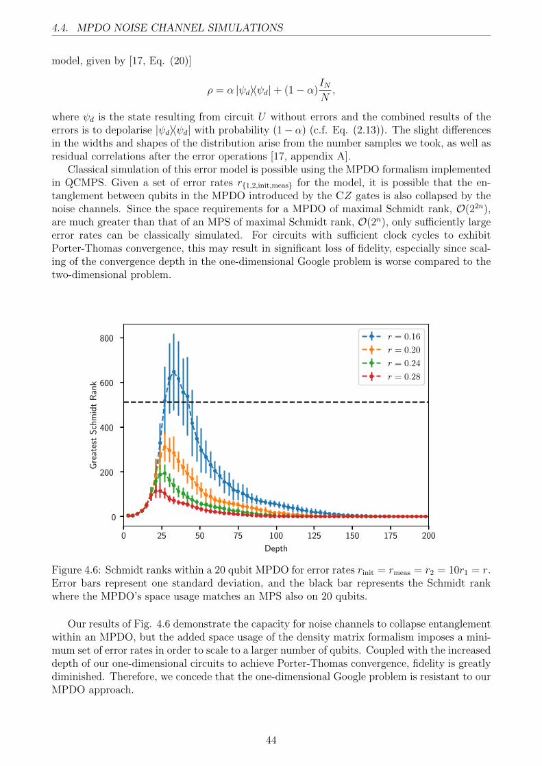
4.4. MPDO NOISE CHANNEL SIMULATIONS
model, given by [17, Eq. (20)]
ρ = α |ψd〉〈ψd|+ (1− α)INN,
where ψd is the state resulting from circuit U without errors and the combined results of theerrors is to depolarise |ψd〉〈ψd| with probability (1− α) (c.f. Eq. (2.13)). The slight differencesin the widths and shapes of the distribution arise from the number samples we took, as well asresidual correlations after the error operations [17, appendix A].
Classical simulation of this error model is possible using the MPDO formalism implementedin QCMPS. Given a set of error rates r{1,2,init,meas} for the model, it is possible that the en-tanglement between qubits in the MPDO introduced by the CZ gates is also collapsed by thenoise channels. Since the space requirements for a MPDO of maximal Schmidt rank, O(22n),are much greater than that of an MPS of maximal Schmidt rank, O(2n), only sufficiently largeerror rates can be classically simulated. For circuits with sufficient clock cycles to exhibitPorter-Thomas convergence, this may result in significant loss of fidelity, especially since scal-ing of the convergence depth in the one-dimensional Google problem is worse compared to thetwo-dimensional problem.
0 25 50 75 100 125 150 175 200
Depth
0
200
400
600
800
GreatestSchmidtRank
r = 0.16
r = 0.20
r = 0.24
r = 0.28
Figure 4.6: Schmidt ranks within a 20 qubit MPDO for error rates rinit = rmeas = r2 = 10r1 = r.Error bars represent one standard deviation, and the black bar represents the Schmidt rankwhere the MPDO’s space usage matches an MPS also on 20 qubits.
Our results of Fig. 4.6 demonstrate the capacity for noise channels to collapse entanglementwithin an MPDO, but the added space usage of the density matrix formalism imposes a mini-mum set of error rates in order to scale to a larger number of qubits. Coupled with the increaseddepth of our one-dimensional circuits to achieve Porter-Thomas convergence, fidelity is greatlydiminished. Therefore, we concede that the one-dimensional Google problem is resistant to ourMPDO approach.
44
Chapter 5
Conclusion
To simulate the circuits of Shor’s algorithm and the Google supremacy problem, we developedthe highly optimised numerical library QCMPS for manipulating matrix product states andmatrix product density operators. Conventionally, it is tailored for simulations of quantumcircuits, but may readily be extended to perform simulations of other algorithms pertinent tocondensed matter physics, such as the density matrix renormalisation group method and time-evolving block decimation. This library introduces several unique features, including moreefficiently simulating specific linear nearest neighbour binarily controlled gates on potentiallymany sites of a pure state. It also uniquely implements the matrix product density operatorformalism for simulating density matrices, allowing error models for the noise and decoherenceeffects experienced by a physical quantum machine to be simulated in a manner that takesadvantage of the scaling in the simulation time and space requirements with respect to en-tanglement. Crucially, QCMPS was developed for distributed memory architectures, allowingit to scale to take advantage of the greater amounts of computational resources provided bysupercomputers or computer clusters.
Building upon previous methods for simulating Shor’s algorithm for semiprime factorisation,we described additional optimisations for our own implementation. Among these optimisationsis the choice of simulating Shor’s algorithm as a sampling problem, mimicking the process bywhich a real quantum computer might extract meaningful information from a quantum stateproduced by Shor’s algorithm. As a sampling problem, the subsequent measurements madeduring the quantum Fourier transform serve to mitigate entanglement introduced by its gates,reducing rather than increasing the space requirements to perform this subroutine of Shor’salgorithm.
By effectively characterising the multipartite entanglement over the course of Shor’s algo-rithm and sensibly mapping it to a matrix product state of linear connectivity, we were ableto refine previous estimates for the required simulation costs that were based on the period rto, instead, the factors of r. The culmination of all our optimisations combined is a successfulsimulation of a specifically chosen 60 qubit instance that previous estimations would have foundextremely difficult space-wise, but one that we would ultimately perform with approximately14 TB of memory over 8 h. Despite being a high-level simulation, this is still potentially thelargest instance of a non-trivial quantum algorithm ever performed.
To extend our simulations of Shor’s algorithm, it would be prudent to consider simulatinga gate-wise decomposed circuit for Shor’s algorithm, particularly decompositions into linearnearest neighbour gates that fit well with the linear connectivity of matrix product states.Doing so would also open the possibility of performing these simulations using the matrixproduct density operator functionality of QCMPS to examine the circuit’s resilience to specificerror models. Additionally, we might also wish to perform these simulations of Shor’s algorithmwhen applied to the discrete logarithm problem as it appears in, say, elliptic curve cryptography.
45
We then turned our sights to Google’s supremacy problem, which involves sampling themeasurement results from the specification of a random circuit. Though the original circuitsuse nearest neighbour gates on 2-dimensional qubit arrays, we decided instead to approachthe one-dimensional versions due to their suitability for our matrix product states and densityoperators.
Ultimately, we found that the amount of gates in a random one-dimensional circuit ofthe Google supremacy problem required for the measurement probabilities to converge to thePorter-Thomas distribution was significantly higher than 2-dimensional circuits over the samenumber of qubits. This increase in the number of gates results in the one-dimensional cir-cuits being less resilient to errors described by the model given by Google, but also to matrixproduct state truncation. We were able to demonstrate this decay in sampling fidelity due tomatrix product state truncation and, separately, Google’s error model involving bit-flip anddepolarising channels. Use of QCMPS’ matrix product density operator functionality allowedus to observe the competing effects of the gates introducing entanglement and the depolarisingchannels collapsing it. For sufficiently high error rates, these circuits are viably simulated butresult in poor sampling fidelity, affirming the one-dimensional Google problem’s resistance toour matrix product methods.
Our goal from here is to extend the functionality of QCMPS by improving its interfaceand implementing better support for general matrix product operators. To achieve featureparity with other existing quantum simulators or tensor network libraries, we might also wishto implement support for general tensor networks, of which matrix product states and matrixproduct operators and density operators form a small subset, and also for increasingly popu-lar heterogeneous GPU-accelerated computing architectures. As it stands, however, QCMPSshould serve as a valuable tool for matrix product simulations of quantum algorithms.
46
Bibliography
1A. M. Turing, “On computable numbers, with an application to the entscheidungsproblem”,Proceedings of the London Mathematical Society s2-42, 230–265 (1937).
2P. W. Shor, “Polynomial-time algorithms for prime factorization and discrete logarithms ona quantum computer”, SIAM Journal on Computing 26, 1484–1509 (1997).
3R. Jozsa and N. Linden, “On the role of entanglement in quantum-computational speed-up”, Proceedings of the Royal Society of London A: Mathematical, Physical and EngineeringSciences 459, 2011–2032 (2003).
4C. H. Bennett, “Notes on landauer’s principle, reversible computation, and maxwell’s demon”,Studies in History and Philosophy of Science Part B: Studies in History and Philosophy ofModern Physics 34, Quantum Information and Computation, 501–510 (2003).
5A. C.-C. Yao, “Quantum circuit complexity”, in Proceedings of 1993 ieee 34th annual foun-dations of computer science (Nov. 1993), pp. 352–361.
6E. Farhi, J. Goldstone, S. Gutmann, and M. Sipser, “Quantum Computation by AdiabaticEvolution”, eprint arXiv:quant-ph/0001106 (2000).
7L. K. Grover, “A fast quantum mechanical algorithm for database search”, in Proceedings ofthe twenty-eighth annual acm symposium on theory of computing, STOC ’96 (1996), pp. 212–219.
8J. Daemen and V. Rijmen, The design of Rijndael: AES — the Advanced Encryption Standard(Springer-Verlag, 2002), p. 238.
9R. L. Rivest, A. Shamir, and L. Adleman, “A method for obtaining digital signatures andpublic-key cryptosystems”, Commun. ACM 21, 120–126 (1978).
10D. J. Bernstein, “Introduction to post-quantum cryptography”, in Post-quantum cryptogra-phy, edited by D. J. Bernstein, J. Buchmann, and E. Dahmen (Springer Berlin Heidelberg,Berlin, Heidelberg, 2009), pp. 1–14.
11A. Montanaro, “Quantum algorithms: an overview”, npj Quantum Information 2, 15023,15023 (2016).
12A. G. Fowler, M. Mariantoni, J. M. Martinis, and A. N. Cleland, “Surface codes: towardspractical large-scale quantum computation”, Phys. Rev. A 86, 032324 (2012).
13A. P. Lund, M. J. Bremner, and T. C. Ralph, “Quantum sampling problems, BosonSamplingand quantum supremacy”, npj Quantum Information 3, 15, 15 (2017).
14B. T. Gard, K. R. Motes, J. P. Olson, P. P. Rohde, and J. P. Dowling, “An introduction toboson-sampling”, in From atomic to mesoscale (WORLD SCIENTIFIC, 2015) Chap. Chapter8, pp. 167–192.
15H. Meuer, E. Strohmaier, J. Dongarra, H. Simon, and M. Meuer, Top500, (Oct. 2017) https://www.top500.org/.
47
BIBLIOGRAPHY
16M. J. Bremner, R. Jozsa, and D. J. Shepherd, “Classical simulation of commuting quantumcomputations implies collapse of the polynomial hierarchy”, Proceedings of the Royal Societyof London A: Mathematical, Physical and Engineering Sciences 467, 459–472 (2010).
17S. Boixo, S. V. Isakov, V. N. Smelyanskiy, R. Babbush, N. Ding, Z. Jiang, M. J. Bremner,J. M. Martinis, and H. Neven, “Characterizing Quantum Supremacy in Near-Term Devices”,ArXiv e-prints (2016).
18J. Johansson, P. Nation, and F. Nori, “Qutip 2: a python framework for the dynamics of openquantum systems”, Computer Physics Communications 184, 1234–1240 (2013).
19M. Smelyanskiy, N. P. D. Sawaya, and A. Aspuru-Guzik, “qHiPSTER: The Quantum HighPerformance Software Testing Environment”, ArXiv e-prints (2016).
20R. Orus, “A practical introduction to tensor networks: matrix product states and projectedentangled pair states”, Annals of Physics 349, 117–158 (2014).
21G. Vidal, “Efficient classical simulation of slightly entangled quantum computations”, Phys.Rev. Lett. 91, 147902 (2003).
22U. Schollwock, “The density-matrix renormalization group in the age of matrix productstates”, Annals of Physics 326, 96–192 (2011).
23G. Vidal, “Classical Simulation of Infinite-Size Quantum Lattice Systems in One SpatialDimension”, Physical Review Letters 98, 070201, 070201 (2007).
24D. S. Wang, C. D. Hill, and L. C. L. Hollenberg, “Simulations of shor’s algorithm using matrixproduct states”, Quantum Information Processing 16, 176 (2017).
25The Pawsey Supercomputing Centre, The pawsey supercomputing centre, (Oct. 2017) https://www.pawsey.org.au/.
26S. van der Walt, S. C. Colbert, and G. Varoquaux, “The numpy array: a structure for efficientnumerical computation”, Computing in Science Engineering 13, 22–30 (2011).
27M. P. Forum, Mpi: a message-passing interface standard, tech. rep. (Knoxville, TN, USA,1994).
28E. Solomonik, D. Matthews, J. R. Hammond, J. F. Stanton, and J. Demmel, “A massivelyparallel tensor contraction framework for coupled-cluster computations”, Journal of Paralleland Distributed Computing 74, 3176–3190 (2014).
29J. A. Calvin and E. F. Valeev, Tiledarray: a general-purpose scalable block-sparse tensorframework, https://github.com/valeevgroup/tiledarray.
30L. Blackford, J. Choi, A. Cleary, E. D’Azevedo, J. Demmel, I. Dhillon, J. Dongarra, S. Ham-marling, G. Henry, A. Petitet, K. Stanley, D. Walker, and R. Whaley, “Scalapack: a linearalgebra library for message-passing computers”, in In siam conference on parallel processing(1997).
31G. Golub and C. Van Loan, Matrix computations, 4th ed., Johns Hopkins Studies in theMathematical Sciences 3 (Johns Hopkins University Press, Dec. 2012).
32J. Poulson, B. Marker, R. A. van de Geijn, J. R. Hammond, and N. A. Romero, “Elemental:a new framework for distributed memory dense matrix computations”, ACM Trans. Math.Softw. 39, 13:1–13:24 (2013).
33E. R. Jessup and D. C. Sorensen, “A parallel algorithm for computing the singular valuedecomposition of a matrix”, SIAM J. Matrix Anal. Appl. 15, 530–548 (1994).
34E. Anderson, Z. Bai, C. Bischof, S. Blackford, J. Demmel, J. Dongarra, J. Du Croz, A.Greenbaum, S. Hammarling, A. McKenney, and D. Sorensen, LAPACK users’ guide, Third(Society for Industrial and Applied Mathematics, Philadelphia, PA, 1999).
48
BIBLIOGRAPHY
35Q. Wang, X. Zhang, Y. Zhang, and Q. Yi, “Augem: automatically generate high performancedense linear algebra kernels on x86 cpus”, in Proceedings of the international conference onhigh performance computing, networking, storage and analysis, SC ’13 (2013), 25:1–25:12.
36K. Woolfe, Matrix product operator simulations of quantum algorithms, Aug. 2015.
37E. D. Napoli, D. Fabregat-Traver, G. Quintana-Ortı, and P. Bientinesi, “Towards an effi-cient use of the blas library for multilinear tensor contractions”, Applied Mathematics andComputation 235, 454–468 (2014).
38Y. Hirata, M. Nakanishi, S. Yamashita, and Y. Nakashima, “An efficient conversion of quan-tum circuits to a linear nearest neighbor architecture”, Quantum Info. Comput. 11, 142–166(2011).
39M. A. Nielsen and I. L. Chuang, Quantum computation and quantum information: 10th an-niversary edition, 10th (Cambridge University Press, New York, NY, USA, 2011).
40J. D. Hunter, “Matplotlib: a 2d graphics environment”, Computing in Science Engineering 9,90–95 (2007).
41Itensor, http://itensor.org (visited on 09/30/2017).
42S. Al-Assam, S. R. Clark, and D. Jaksch, “The Tensor Network Theory Library”, ArXive-prints (2016).
43T. Dierks and E. Rescorla, The transport layer security (tls) protocol version 1.2, RFC 5246,http://www.rfc-editor.org/rfc/rfc5246.txt (RFC Editor, Aug. 2008).
44A. G. Fowler, S. J. Devitt, and L. C. L. Hollenberg, “Implementation of shor’s algorithm ona linear nearest neighbour qubit array”, Quantum Info. Comput. 4, 237–251 (2004).
45M. Frigo, “A fast fourier transform compiler”, SIGPLAN Not. 39, 642–655 (2004).
46R. L. Graham, T. S. Woodall, and J. M. Squyres, “Open mpi: a flexible high performancempi”, in Parallel processing and applied mathematics: 6th international conference, ppam2005, poznan, poland, september 11-14, 2005, revised selected papers, edited by R. Wyrzykowski,J. Dongarra, N. Meyer, and J. Wasniewski (Springer Berlin Heidelberg, Berlin, Heidelberg,2006), pp. 228–239.
47S. Beauregard, “Circuit for Shor’s algorithm using 2n+3 qubits”, eprint arXiv:quant-ph/0205095(2002).
48C. Zalka, “Fast versions of Shor’s quantum factoring algorithm”, eprint arXiv:quant-ph/9806084(1998).
49P. Gossett, “Quantum Carry-Save Arithmetic”, eprint arXiv:quant-ph/9808061 (1998).
50J. Proos and C. Zalka, “Shor’s discrete logarithm quantum algorithm for elliptic curves”,Quantum Info. Comput. 3, 317–344 (2003).
51S. Aaronson, “P?= NP”, in Open problems in mathematics, edited by J. F. Nash Jr. and
M. T. Rassias (Springer International Publishing, Cham, 2016), pp. 1–122.
52S. Aaronson and A. Arkhipov, “The computational complexity of linear optics”, in Proceed-ings of the forty-third annual acm symposium on theory of computing, STOC ’11 (2011),pp. 333–342.
49