AD/A-000 575

TURBULENCE-MODEL TRANSITION PREDICTIONS FOR BLUNT-BODY FLOWS

David C. Wilcox

DCW Industries

Prepared for:

Air Force Office of Scientific Research

July 1974

DISTRIBUTED BY:

KUJI National Technical Information Service U. S. DEPARTMENT OF COMMERCE

■■■■ WKmm

UNCLASSIFIED ^SECURITY CL»SStnCATICN OF THIS P'J.E Whff Cat» Enlerrri)

REPORT DOCUMENTATION PAGE READ INSTRUCTIONS BEFORE COMPLETINO FORM

I. REPORT NUMBER

AR)SR-m- 74^/71 4 2. COVT ACCESSION NO 3. RECIPIENT'S CATALOG NUMBER

4. TITLE (ltd Subtllf)

TURBULENCE-MODEL TRANSITION PREDICTIONS FOR BLUNT- iODY FLOWS

B. TYPE OF REPORT ft PERIOD COVERED

INTERIM

ÖClWS-SS-'öf 0RG° REPORT NUMBER

AUTHORr«;

bAVID C WILCOX

9. CONTRACT OR GRANT NUMBERf«,)

F44620-74-C-0048

PERFORMING ORGANIZATION NAME AND ADDRESS DCW INDUSTRIES 13534 VALLEY VISTA BOULEVARD SHERMAN OAKS, CALIFORNIA 91403

»0. PROGRAM ELEMENT. PROJECT. TASK AREA « WORK UNIT NUMBERS

681307 9781-02 611Q2F

II. CONTROLLING OFFICE NAME AND ADDRESS

AIR FORCE OFFICE OF SCIENTIFIC RESEARCH/NA 1400 WILSON BOULEVARD ARLINGTON, VIRGINIA 22209

12. REPORT DATE July 1974 IS. NUMBER OF PAGES

U. MONITORING AGENCY NAME A AODRESSC'/ dilltfnl Irom CentiolUni Olllet) IS. SECURITY CLASS, (at Ihlt nport)

UNCLASSIFIED ISa. OECLASSIFICATION/DOWN GRADING

SCHEDULE

14. DISTRIBUTION STATEMENT (of Ihli Rtpert)

Approved for public release; distribution unlimited.

17. DISTRIBUTION STATEMENT (ol Ml« abiifct »nltfd In Block 30, II dillntnt Inm Rtpott)

14. SUPPLEMENTARY NOTES

Reproduced by NATIONAL TECHNICAL INFÖRMAriON SERVICE U S Department of Commerce

Springfiel:' VA Z2151

. .n\

It. KEY WORDS (Contlnu» en »verae (Id* II neeeeawy arid Identity by block number)

BOUNDARY LAYER TRANSITION TURBULENCE PREDICTION TRANSITION PREDICTION BLUNT-BODY FLOWS RE-ENTRY AEROMECHANICS 20. ABSTRACT (Continue on reveraa aid« II neeeiemty and Identify by b ock number)

An accurate and efficient method has been developed for predictin!., transition from laminar to turbulent flow. The method is based upon a phenomenoiogical turbulence model originally devised by Saffman for fully turbulent flows. The model is modified to account for low Reynolds number phenomena and is used to make a priori transition predictions. Primary emphasis focuses upon blunt-bodv flows; predict ons are also made for consLant-prcssure boundary-layer flows Lo provide as broad a data base as possible to assess model accuracy. The method yields excellent agreement between computed and experimentally measured effects

DD,^NRM7i 1473 EDITION OF I NOV 65 IS OBSOLETE

/ UNCLASSIFIED SECURITY CLASSIFICATION OF THIS PAGE iWirn /)«(• Bntered

UNCLASSTFTED teCUJ"»V CLASSIFICATION OP THIS PAGEfHTi«V>«>« Enmfd)

of freedsteam turbulence, surface roughness and suction on Incompressible 1'lat- plate-boundary-layer transition. Model-predicted effects of surface roughness on transition in the vicinity of the stagnation point of a sphere-cone body

rtually duplicate measured effects. The method also yields close agreement oetween calculated and measured surface-cooling and nose-radius effects on sphere cone transition. Based on results obtained in the study, a blunt-body transitioi prediction algorithm for use by weapon-system design engineers has been devised.

f a.

UNCLASSIFIED

"

SECURITY CLASSiriCATIC'J Of THIS PAfiF'^hrn Du» Unfrrnä)

I \ POREWORD

This report summarizes research performed In Contract

P44620-71*-C-00^8 during the period January 15 through July 15t 1974. The research was Jointly sponsored by the Space and Missile Systems Organization and the Air Force

Office of Scientific Research (AFSC), United States Air Force. The Air Force program monitors were Captain A.R. Hunt and Second Lieutenant T. Hopkins of SAMSO and Dr. M. Rogers of AFOSR. Mr. W. Portenier maintained technical liason with the Aerospace Corporation.

Participants in the study were D.C. Wilcox, principal investigator, and T.L. Chambers. Manuscript preparation was supported by B.A. Wilcox, W.A. Coonfield, and G.J. McCornock. Professor P.O. Saffman of the California In- stitute of Technology also made important contributions during the course of the study.

A technical note based on results obtained in this study has been submitted for publication in the AIAA Journal. The note is entitiled, "Turbulence-Model Transition Predic- tions" and is authored by D.C. Wilcox. Material presented in the note includes, with the exception of surface rough- ness effects, all significant results presented in Sections

2 and 3.

A second AIAA Journal publication is in preparation. The paper will be based on the surface-roughness analyses of Sections 3 and 4.

ii

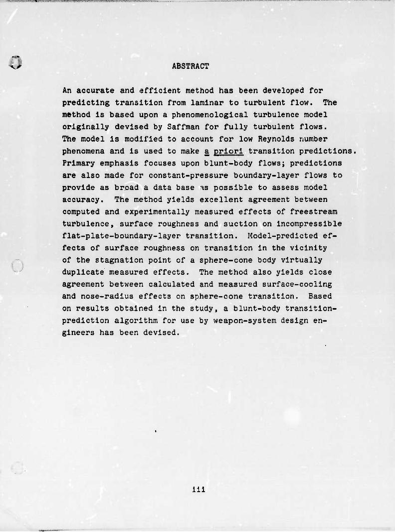
5 ABSTRACT

An accurate and efficient method has been developed for

predicting transition from laminar to turbulent flow. The

method is based upon a phenomenological turbulence model

originally devised by Saffman for fully turbulent flows.

The model is modified to account for low Reynolds number

phenomena and is used to make a priori transition predictions,

Primary emphasis focuses upon blunt-body flows; predictions

are also made for constant-pressure boundary-layer flows to

provide as broad a data base as possible to assess model

accuracy. The method yields excellent agreement between

computed and experimentally measured effects of freestream

turbulence, surface roughness and suction on incompressible

flat-plate-boundary-layer transition. Model-predicted ef-

fects of surface roughness on transition in the vicinity

of the stagnation point of a sphere-cone body virtually

duplicate measured effects. The method also yields close

agreement between calculated and measured surface-cooling

and nose-radius effects on sphere-cone transition. Based

on results obtained in the study, a blunt-body transition-

prediction algorithm for use by weapon-system design en-

gineers has been devised.

Ill

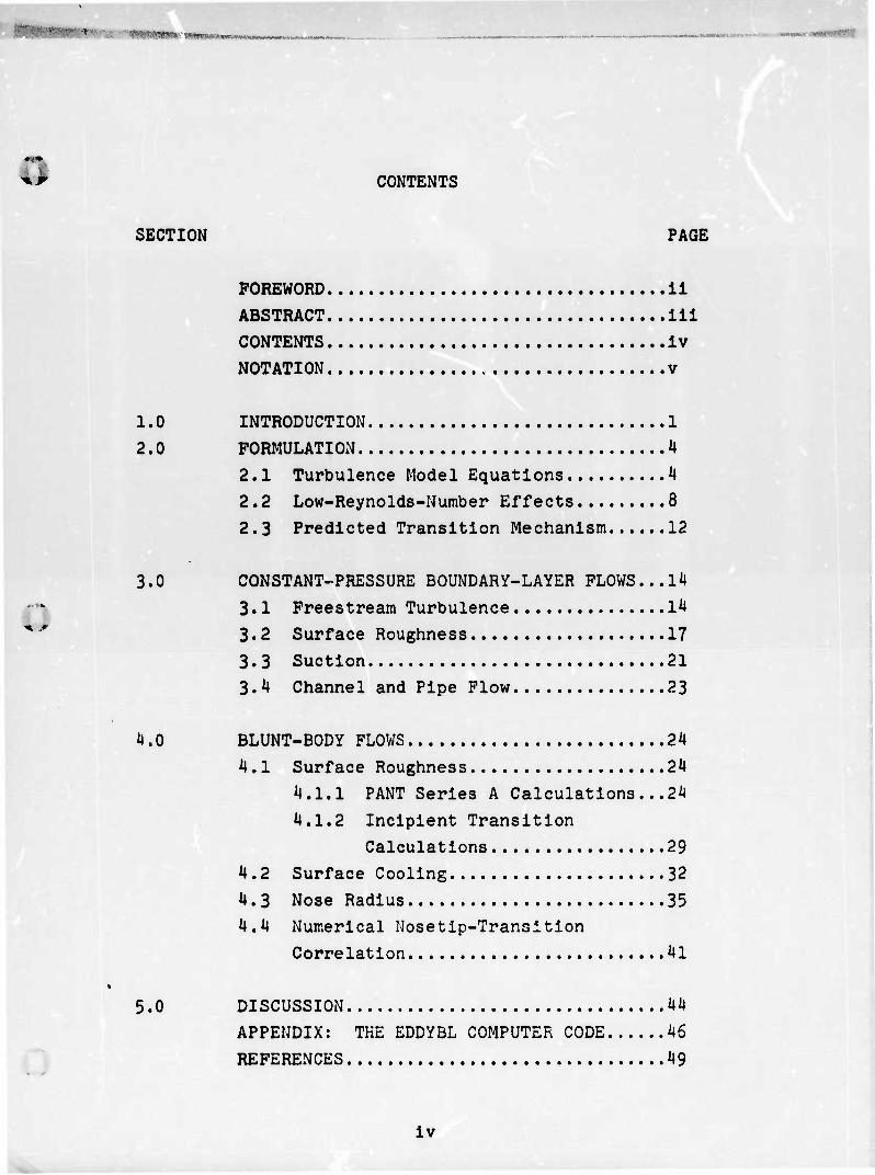
:; CONTENTS

SECTION PAGE

FOREWORD ii ABSTRACT Ill

CONTENTS iv

NOTATION v

1.0 INTRODUCTION 1

2.0 FORMULATION 1

2.1 Turbulence Model Equations ^1

2.2 Low-Reynolds-Number Effects 8

2.3 Predicted Transition Mechanism 12

3.0 CONSTANT-PRESSURE BOUNDARY-LAYER FLOWS... 1^1

3.1 Freestream Turbulence I1*

3.2 Surface Roughness 17

3.3 Suction 21

3.^1 Channel and Pipe Flow 23

M BLUNT-BODY FLOWS 24

H . 1 Surface Roughness 24

4.1.1 PANT Series A Calculations...24

4.1.2 Incipient Transition

Calculations 29

4 .2 Surface Cooling 32

4. 3 Nose Radius 35

4.4 Numerical Mosetlp-Transition

Correlation 41

5.0 DISCUSSION 44

APPENDIX: THE EDDYBL COMPUTER CODE 46

REFERENCES 49

iv

NOTATION

SYMBOL DEFINITION

e

J k N

N(k/e)

P,Pt

rI q» q

PrL, PrT

stag

AN

Re, Re!

S(kuT/v) T T

T'

u

V

X

y

Rex, Ree

U

Skin friction Specific heat at constant pressure

Volume coefficient

Specific turbulent energy

Index for planar (J=0) or axisymmetrlc (J«l) flow

Roughness height

Mach number

Surface-roughness function

Static pressure, total pressure

Laminar and turbulent Prandtl number

Local heat transfer, stagnation-point heat transfer

Radial body coordinate Nose radius

Freestream unit Reynolds number

Reynolds number based on roughness height, plate length, momentum thickness Turbulent Reynolds number

Neutral-stability Reynolds number

Empirical parameter In Saffman turbulence model

Arc length Surface-roughness function

Static temperature, total temperature

Turbulence Intensity at boundary-layer edge

Velocity component In x direction

Boundary-layer-edge velocity, freestream velocity

Velocity component in y direction

Coordinate lying along a solid body

Coordinate normal to a solid body

Empirical parameters in Saffman turbulence model

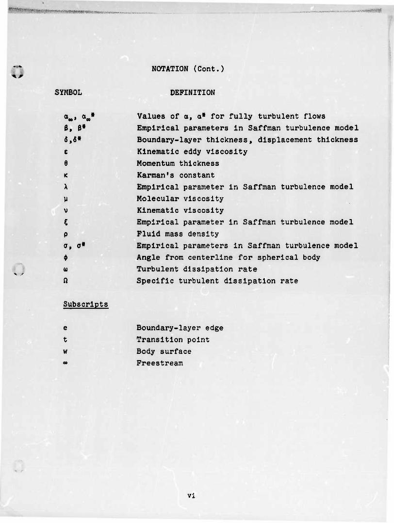
NOTATION (Cont.)

SYMBOL DEFINITION

e, e» 6,6»

e

e K

X

u V

P O, 0*

u

Q

Values of o, a* for fully turbulent flows

Empirical parameters in Saffman turbulence model

Boundary-layer thickness, displacement thickness

Kinematic eddy viscosity

Momentum thickness

Karman's constant

Empirical parameter in Saffman turbulence model

Molecular viscosity

Kinematic viscosity

Empirical parameter in Saffman turbulence model

Fluid mass density

Empirical parameters in Saffman turbulence model

Angle from centerline for spherical body

Turbulent dissipation rate

Specific turbulent dissipation rate

Subscripts

e

t

w

Boundary-layer edge

Transition point

Body surface

Freestream

vi

0 1.0 INTRODUCTION

An understanding of boundary-layer transition phenomena in

blunt-body flows is essential to the design of reentry-

vehicle nosetips. Transition sensitivity to many complicated

effects must be defined; these effects include surface rough-

ness, surface cooling, mass transfer, nosetip geometry, free-

stream Mach number, and freestream turbulence level. Although 1-7 experimental work ' has attempted to quantify the importance

of these various effects, a reliable analytical tool for pre-

dicting complex-flow transition-point location remains to be

developed. Since flight conditions often cannot be simulated

accurately in a wind tunnel and since applicable, retrievable

flight-test data are rare, accurate analytical tools are needed

to facilitate extrapolation from wind-tunnel conditions to

real flight conditions.

Although analytical tools for predicting transition from laminar

to turbulent flow have improved significantly in recent years,

transition remains one of the least-understood phenomena of

fluid mechanics. Presently, analytical studies focus on the

following four approaches:

1. Semiempirical Formulas

The simplest approach Is to start with a physical fact

or argument and devise a formula containing adjustable

parameters; a classic example of this method Is given 0

by Van Driest and Blumer . Such formulas can be very

useful for parametric studies and for correlating ex-

perimental data for a given class of flows, but a lack

of universality generally limits th* utility of this

approach.

2. First Principles

The most rigorous tact that can be taken is to seek

-1-

:;

time-dependent Navier-Stokes solutions. While pre- o

llminary steps have been taken in this direction ,

required computing times are currently too lengthy

to make such computations practicable for engineer-

ing applications.

3. Linear Stability Analysis

The approach which has received the greatest amount

of attention is linear stability analysis ^.

While some insight into the transition phenomenon

has attended this work, predictions often differ from

experimental observations. Furthermore, linear anal-

ysis determines stability of a flow to infinitesimal

disturbances only and is inapplicable when initial

flow perturbations are of finite amplitude. Finally,

in a linear stability analysis, complicating effects

such as wall roughness, wall colling, mass transfer,

and freestream turbulence level and scale consider-

ably increase the approach's mathematical complexity.

4. Phenomenological Turbulence Models

A relatively new method offers many advantages over

the approaches listed above; this method uses the

Reynolds-averaged equations of notion subject to a

set of closure hypotheses suitable for accurate com-

putation through transition. This approach, on the

one hand, is applicable to arbitrary amplitude dis-

turbances and, on the other hand, in a simple and

natural way can account for the complicating effects

cited above. Recent progress with phenomenologlcal-

turbulence-model equations indicates this approach is

sensible, i.e., that adequate closure approximations

can indeed be determined. Using turbulence-model

equations in which the Reynolds stresses depend upon

-2-

flow history, Donaldson , Jones and Launder , and

Wllcox have shown that such equations accurately

predict abrupt transition from laminar to turbulent

flow for constant-pressure boundary layers.

The turbulence-model approach is taken in the present

study, where the primary objective has been to develop an

accurate method for predicting transition in blunt-body

flows, including the effects of surface roughness, sur-

face cooling, mass transfer, blunt-body geometry, free-

stream Mach number, and freestream turbulence. To accom-

plish this objective, a series of transition-prediction

computations has been performed based on the Saffman 19 turbulence-model equations . To provide a broad data

base for assessing turbulence-equation accuracy, the cal-

culations Include transitional flat-plate-boundary-layer

(FPBL), pipe, and channel flow In addition to the more-

pertinent blunt-body-flow computations. Section 2 dis-

cusses the model equations and the method by which transi-

tion predictions are made; qualitative features of the

model-predicted transition mechanism are also described.

Section 3 presents transition predictions for constant-

pressure boundary-layer flows and includes comparisons

with experimental data. Section h summarizes transition

predictions for blunt-body flows; based on the results

presented in Section 4, a new engineering correlation is

devised which can be used for predicting nosetip transi-

tion. Results of the study are summarized in Section 5.

-3-

2.0 FORMULATION

The basic analytical approach taken in the study for pre-

dicting transition Is presented In this section. Subsection

2.1 presents the turbulence model equations and the method

by which the equations are used to predict transition. Model

revisions required for Improving transition-prediction ac-

curacy are described In Subsection 2.2. The section concludes

with a discussion of the model-predicted transition mechanism.

2.1 TURBULENCE MODEL EQUATIONS

The turbulence model equations which form the basis of 17 the present study were originally devised by Saffman for

incompressible flows. In subsequent development efforts * , Wilcox has cast the model equations in a form suitable for

compressible flow applications. The Saffman model is a two-

equation model of turbulence; i.e., two nonlinear diffusion

equations are solved in addition to the conservation (mass, momentum, energy) equations in computing a given flowfield.

20 In terms of mass-averaged mean quantities , the coupled set

of equations describing compressible boundary-layer flows

over planar (J=0) or axisymmetric (J=l) surface are as follows:

Conservation of Mass

^(rJpu) + ^(rV) = 0 (1)

Conservation of Momentan

pU|ü + pvla = d££ + i -lcrJ(w+e/ro|#3 (2) M ax ^ 5y dx rJ 9yL vw ' ^y- v y

.4-

,:

Conservation of Energy

pu^OpT) + PV^CCpT) = ufEs + (u+e/n)(|H)

*k4^^+^4%T''] (3) rL ^rqi

Specific Turbulent Energy

+ FT 37 CrJ (M+^Vfl)!»] (»)

Specific Turbulent Dissipation Rate

""If + ^lr - C«l|fl - Bpn]pn!

+ ir äl CrJ (^«/n)||i] (5)

In Equations (1-5), x and y are orthogonal coordinates with

x lying along the body and y being normal to the surface; r

Is the radial body coordinate (see Figure 1). Velocity

components In the x and y directions are denoted by u and v.

The quantities p, p, and T denote pressure, density, and

temperature. Molecular viscosity is the quantity y while

the eddy viscosity is given by e/n, the ratio of specific

turbulent energy, e, to specific dissipation rate,n. Lami-

nar and turbulent Prandtl numbers, PrL and Prip» appear in

Equation (3) while seven empirical parameters (a,a*,8,B*,a,

a*,5) are contained in Equations (4 and 5). Subscript e de-

notes the value of a quantity at the boundary-layer edge.

With the exception of £, values of the empirical parameters

and the turbulent Prandtl number are regarded as universal

constants for fully developed turbulent flows, and their

-5-

Shock wave

Figure 1. Coordinate system and notation,

-6-

values have been established by general arguments based on 17-19 well-documented experimental observations for such flows

The value of ^ has been selected by comparison of model pre-

dictions with experimental data for a variety of supersonic i p

and hypersonic flows . In all past calculations, values

for these constants have been given by:

s 2. 50

a» ■ 0. 50

8« ■ 0. 09 a« = a* = 00 0.30

0 s 0. 50

0 .15 < ß < C .18

a ■ a« j a»[ß/3» - 4aic2/a*]

(6)

where K = 0.41 is the Karman constant.

In solving Equations (1-5), values of u, T, e and ß are

prescribed at the boundary-layer edge. The no-slip velocity

boundary condition is Imposed at y = 0 while either sur-

face temperature or surface heat flux is given. Turbulent

energy vanishes at y = 0 and, for perfectly smooth surfaces' ,

y2n ■ 20y/3p2 (the boundary condition for ß appropriate on

a rough surface is discussed in Subsection 3.2).

.19

The Saffman turbulence model has been incorporated in a boundary-layer program developed at the NASA Langley Research

21 Center ; the modified program is known as EDDYBL (see Ap- pendix). In using EDDYBL to make boundary-layer transition predictions, specific turbulent energy and specific dissipa- tion rate are held constant at the boundary-layer edge. Turbulent energy is set to sero throughout the boundary layer at a point near the plate leading edge. Solution of the parabolic system is accomplished by marching in the stream-

-7-

')

wise direction. Some entralnment and molecular diffusion

of turbulent energy, e, into the boundary layer initially

occurs; however little or no turbulent-energy amplification

occurs for a plate-length Reynolds number below a critical

value Rex , signifying existence of laminar flow. Then,

when Rex * Rext» an abrupt increase in e is observed, fol- lowed by an asymptote to a value characteristic of fully

developed turbulent flow. The transitional regime is

readily identified as the range over which e increases from

its initially low level to its much higher value in the

turbulent regime. The transitional regime can also be iden-

tified from the numerical data by locating abrupt changes

in quantities such as momentum thickness, shape factor, and

skin friction.

2.2 LOW-REYNOLDS-NUMBER-EFFECTS

In an earlier study , the Saffman model showed promise of

being an accurate tool for transition prediction. Using

the values of the empirical parameters given in Equation (6),

transition was predicted for Rayleigh shear flow. Although

experimental data are not available for transitional Ray-

leigh flow, the computed transition appeared realistic as

computed Raylelgh-flow properties and measured FPEL proper-

ties were in close quantitative agreement. The first calcu-

lation in the present study was for PPBL flow so that more-

direct comparison could be made between model predictions

and experimental data.

Figure 2 shows computed skin friction, c«, as a function of

Re for an incompressible FPBL. The freestream value of -9 2 e is 10 U , where U is freestream velocity. As shown,

the predicted transition begins at Re = ^«lO1* and ends at

Re = 105. The predicted value of ReXl. of k*l& is much

lower than the measured Rex for very low freestrear; tur-

-8-

u

s tt o H E-< H < CO J 2

S O Ü

K O *

s Ü 0 o m H w 0 tH X !=> D •J o • 9

O 2 a W H w

1 ^ CO CO < D ■ a H H D to Ui o < CU 1-5 J o < OQ X o

< 4

6H Ü O m

o

0) 0)

I •p I i

cd

o c • OtJ •H m -P OH O fc

3 0) «MrH

01 SCO

a» u c a o e

•H O .P O O ß •H TH

<M C CO

c •H ^ JsJ O CO *H

0)

3 bO

-9-

5 bulence levels; Schubauer and Skramstad , for example.

indicate that Rex. should be nearly 3'lO6 for ee ^ 10"'U -7M2

e

Assuming a,o*,B,8*,o,a*>C are Independent of Reynolds number

leads to the Inaccuracy. As noted above, the values for

the empirical parameters in Equation (6) are presumed valid

for fully developed turbulent flows; however, there is no

a priori reason why these parameters should be independent 22 of Reynolds number. In fact, Rotta argues that such

parameters depend directly upon the turbulence spectrum;

since the turbulence spectrum will be quite different for

low-Reynolds-number turbulence, Rotta's argument suggests

that a,a*, etc, should be Reynolds-number-dependent. Other 15 investigators have, in fact, introduced a functional de-

pendence of similar parameters upon turbulent Reynolds num-

ber ReT = e/ßy. In the present study, transition is found

most sensitive to the values of a and a*; decreasing a*

tends to delay transition while the ratio of a to a* fixes

the width of the transition zone; therefore to improve tran-

sition-prediction accuracy, an assumption is made that

a« = o» [1 - (l-A)(l-ReT/Ro)K(l-ReT/Ro)] (7)

a/a« = ayo« (8)

where H(x) Is the Keaviside steofunction and a and a* are 00 00

the values of a and a* appropriate for fully turbulent flows

[see Equation (6)].

The value of \ can be fixed by demanding that the Saffman-

model neutral stability Reynolds number. Re , for a Blasius

boundary layer be the same as that predicted by linear

stability theory. Neutral stability for the turbulence

model is defined as the condition where a*|3u/3y| ■ ß*u)

-10-

where u is turbulent dissipation rate given by a» = pfl. Then,

using the Blasius velocity profile and a computed w-profile

leads to

Rex » 1000/A2 (9)

with the least stable point being at appro:imately y/6 = 0.30.

Hence, using the accepted linear stability value of Re of

9,105, A ■ 0.105. A similar argument for selecting the value

of R remains to be found. Numerical experimentation indi-

cates that IL should be about 0.10, but this value should o be regarded as tentative until further applications are

made to determine its universality.

Finally, regarding the turbulence model and its application

to transitional flows, note that algebraic transition pre-

dictions can be made which apparently are accurate to within

a factor of two or three. Specifically, for many incompres-

sible laminar flows over perfectly smooth surfaces, w is

given by w » 20v/ßy2 so that neutral stability occurs when

y2|3u/ay|/v=20/(Aaȧ/6*) = 517. Also, transition will be

complete when production of w2 exceeds to2 dissipation, i.e.,

when y2|3u/3y|/v = 20/(Aa*) = 722. Therefore, an approximate

transition criterion predicted by the model for incompressible

flows is

317 < m^X y2|au/3y|/v < 722 (10)

Q

Equation (10) resembles the Van Drlest-Bluner formulation.

When dealing with incompressible flows In this study, the turbulent dissipation rate, w, Is used in place of the speci- fic turbulent dissipation rate,?..

-11-

% p

2.3 PREDICTED TRANSITION MECHANISM

Before discussing results obtained in the present study for

constant-pressure boundary-layer flows (Section 3) and

blunt-body flows (Section 4), it is interesting to pause

and discuss the model-predicted transition mechanism. The

most-thoroughly studied flow with regard to transition is

probably incompressible FPBL flow; therefore, discussion

below concentrates upon the Blasius boundary layer.

As noted in Subsection 2.1, starting from the plate leading

edge with e = 0 throughout the boundary layer and maintain-

ing e = e and u = w at the boundary-layer edge (y = 6),

a small amount of turbulent energy is entrained beginning

at the plate leading edge. This turbulent energy then

spreads through the boundary layer by the action of molecu-

lar diffusion. At this point, the turbulent energy in-

creases monatonically from zero at the plate surface to its

freestream value at the boundary-layer edge.

No turbulent-energy amplification occurs for a significant

distance downstream of the plate leading edge. Turbulent-

energy entrainment continues and, just upstream of the

neutral stability point, a spike, or local maximum, deve-

lops in the e-proflle for y/6 between 0.^5 and 0.60, de-

pending upon the value of w . This prediction is consis-

tent with experimental measurements which indicates that

disturbances are first amplified in a Blasius boundary

layer at a point located about 60!^ of the way through the

boundary layer. :.'o effect on skin friction, shape factor,

etc, is observed at this point. The spike diffuses toward

the wall with the magnitude of the spike remaining approx-

imately constant; then, beyond the neutral-stability point,

the spike is gradually amplified. Finally, at a plate-

length Reynolds number Rex , an abrupt increase in e is

-12-

observed throughout the boundary layer. Indicating the on-

set of transition. The spike is now located at y/6 = 0.2,

near the critical layer. This prediction is consistent

with linear stability analysis which indicates the lease-

stable point in a Blasius boundary layer occurs in the

critical layer. Turbulent energy is amplified to a value

typical of fully turbulent flow and levels off when Re

is two or three times Rext. The width of the transitional

region is realistic as Rex is observed experimentally to

increase typically by a similar amount through transition.

Hence, many qualitative features of FPBL transition are

adequately represented in the model-predicted transition.

As will be shown in the following sections, the model

also yields accurate quantitative predictions for proper-

ties of engineering interest (e.g., transition Reynolds

number) in both FPBL and blunt-body flows.

-13-

3.0 CONSTANT-PRESSURE BOUNDARY-LAYER FLOWS

This study*s primary objective has been to develop an

accurate transition-prediction method for blunt-body

(e.g., RV nosetips) flows. However, a wealth of constant-

pressure boundary-layer-transltlon data is available, in-

cluding many effects pertinent to transition on reentry

vehicles (RV's) under flight conditions. Hence, studying

botn constant-pressure boundary-layer and blunt-body flows

permits a larger data base for testing model accuracy.

Additionally, studying more than one class of flows may

permit development of a universally applicable transition-

prediction method. Calculations have thus been performed

for PPBL flow, channel flow and pipe flow in addition to

the more-pertinent blunt-body flows. Sensitivity of

model-predicted transition for PPBL flow to freestream

turbulence (Subsection 3.1)> to surface roughness (Sub-

section 3.2), and to suction (Subsection 3.3) is deter-

mined. Channel and pipe flow are analyzed in Subsection

3.4.

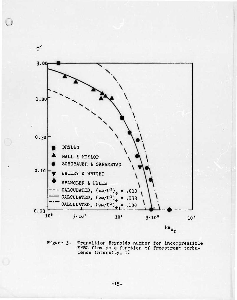
3.1 PREESTREAM TURBULENCE

With o and o* given by Equations (7 and 8), effects of

freestream turbulence on incompressible PPBL transition

have been analyzed. Table 1 summarizes the computations;

Pigure 3 compares model-predicted transition Reynolds

number, R^xt» with experimental datap* 2~ . Transition Reynolds number Is defined In the computations as the

point where cf Is first observed to deviate from the lam-

inar value by more than 0.5%i turbulence Intensity, T1,

is defined as

V?v 100 t/f ea/Ue (11)

-Ik-

1.00

0.30 -

0.10

0.03

T

DRYDEN

HALL & HISLOP

SCHUBAUER & SKRAMSTAD

BAILEY & WRIGHT

SPANGLER & WELLS

CALCULATED, (vw/U2) = .010 CALCULATED, (vw/U2) CALCULATED, (vu/U2) I . LL

.033

.100

10! 3'105 106 3*106

Re.

107

Figure 3. Transition Reynolds number for incompressible PPBL flow as a function of freestream turbu- lence intensity, T'

-15-

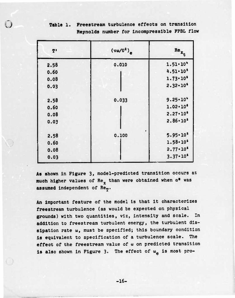
u Table 1. Preeatream turbulence effects on transition

Reynolds number for Incompressible PPBL flow

ft (va)/U2)e Rex xt

2.58 0.010 LSl'lO*

0.60 4.51'105

0.08 1.73-10s

0.03 2.32-106

2.58 0.033 9.25•10,,

0.60 1.02»106

0.08 2.27-106

0.03 2.86-106

2.58 »

0.100 5.95«10s

0.60 1.58-106

0.08 2.77«106

0.03 3.37«10s

As shown in Figure 3, model-predicted transition occurs at

much higher values of Rex 1

assumed independent of Re^.

much higher values of Re than were obtained when o» was

An important feature of the model is that it characterizes

freestream turbulence (as would be expected on physical

grounds) with two quantities, viz, intensity and scale. In

addition to freestream turbulent energy, the turbulent dis-

sipation rate w, must be specified; this boundary condition

Is equivalent to specification of a turbulence scale. The

effect of the freestream value of u on predicted transition

is also shown in Figure 3. The effect of u is most pro-

-16-

nounced for high-Intensity turbulence, with Increasing u tending to delay transition. Excellent agreement with all

data shown Is obtained when vw /U » .033.

3.2 SURFACE ROUGHNESS

Surface roughness has been represented with the turbulence 17 model ' for fully developed turbulent flows by using the

following dissipation rate boundary condition:

« - |F ^ at y - 0 (12)

where uT Is friction velocity and S Is a function of surface 19 roughness. Saffman and Wllcox * have correlated S with

roughness height, k, and arrived at the relation

kuT/v « 50 S~1/2 (13)

Combining Equations (12 and 13) there follows

„.2100^ at y . 0 (li|)

Equation (14) has been developed with the hypothesis that

the roughness element Is very small compared to a typical boundary layer dimension such as momentum thickness, 9. This hypothesis is valid for roughness heights of practical inter-

est (i.e., roughness-height Reynolds number, Re^, up to 1000) when a boundary layer is turbulent. However, for laminar

boundary layers, even relatively small roughness heights will be comparable to the boundary-layer thickness. For example, when Re. > 150, a roughness element is more than lOf» of the boundary-layer thickness when Re ■ 105, a clear violation of the original postulates made in arriving at Equation (lU).

-17-

A more general boundary condition has been devised In the present study, namely,

«- - Sff mm fr M)

where

N(k/e) * 1 as k/e * 0 (16)

To help deduce the functional dependence of N upon k/e,

a simple correlation between Re^ and the value of u at

a solid boundary has been Inferred from experimental data 7

of Pelndt1 for Incompressible rough-wall PPBL flow. The

correlation was developed by numerical experimentation

which showed that the Felndt data are duplicated by model-

equation predictions using the generalized boundary con-

dition (15) with the quantity N given by

N - i| [120/Rek]6 (17)

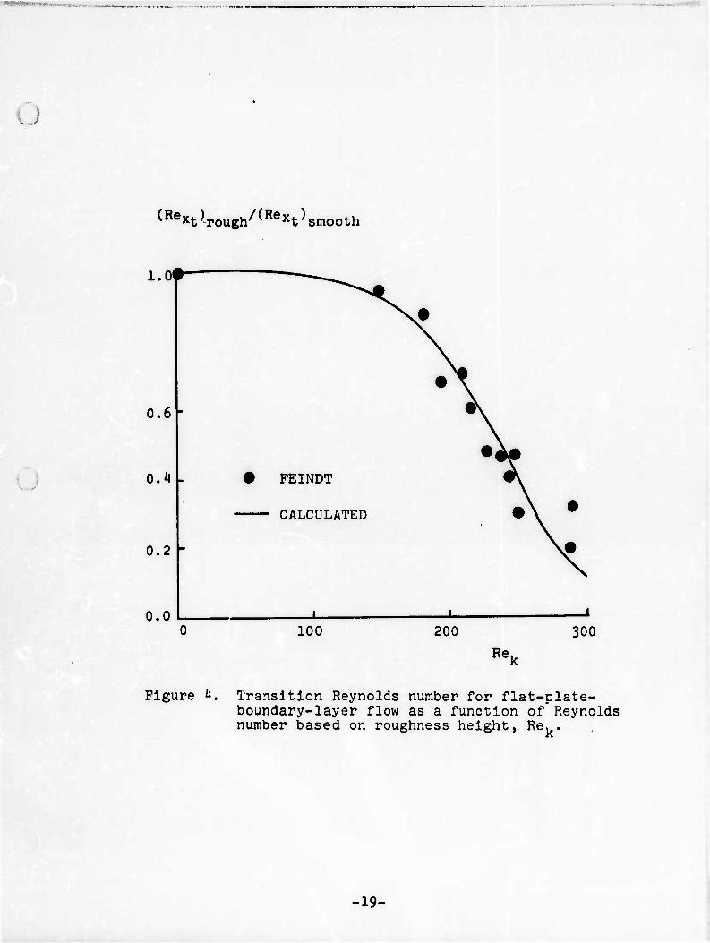
Figure ^ shows the model predicted effect of surface rough-

ness on PPBL transition when Equation (17) is used. Cal-

culations were performed with T' ■ 1% and (vw/U)0 ■ .033;

rebults of the calculations are listed in Table 2.

While excellent agreement with experimental data has been

obtained using Equation (17), the formulation is not quite

complete; that is, the form of the experimental data makes

it convenient to infer N directly as a function of Re^.

While Re^ is certainly of importance in rough-wall tran-

sition, k/9 is a more fundamental parameter since it

provides a criterion for specifying when a roughness

element is large compared to boundary-layer thickness while

the roughness-height Reynolds number Rek does not. How-

-18-

(Rext^ rough/(Rext) smooth

1.0<

0.6

0.4

0.2

0.0

FEINDT

CALCULATED

100 200 300 Re,

Figure H. Transition Reynolds number for flat-plate- boundary-layer flow as a function of Reynolds number based on roughness height. Re,.

-19-

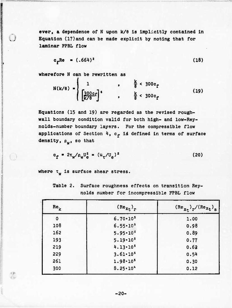
ever, a dependence of N upon k/6 Is Implicitly contained in

Equation (17)and can be made explicit by noting that for

laminar FPBL flow

cfRe - (.66i|)2 (18)

wherefore N can be rewritten as

N(k/e) w f < 300cf

| < 300cf

(19)

Equations (15 and 19) are regarded as the revised rough- wall boundary condition valid for both high- and low-Rey- nolds-number boundary layers. For the compressible flow applications of Section 4, c- iä defined in terms of surface

V density, p , so that

2VPwUe (uT/Ue)2 (20)

where T is surface shear stress.

f

Table 2. Surface roughness effects on transition Rey-

nolds number for incompressible FPBL flow

Rek (Rext>r (ReXt)r/(ReXt)s

' o 6.70«105 1.00

! 108 6.55'105 0.98

[ l62 5.95'105 0.89

193 5.19'105 0.77

219 4.13'105 0.62

229 3.6l«105 O.S4»

261 1.98«105 0.30

300 8.25'10- 0.12

-20-

3.3 SUCTION

Applications In the preceding two subsections have served

mainly to fix the value of the empirical constant R

[Equation (7)] and to determine the analytical dependence

of the function N upon k/e [Equations (15, 19, and 20]. To test the modified turbulence model with no further

parameter adjustment, the effects of suction on FPBL

transition have been analyzed. Computations have been

performed for several suction rates (Table 3) to deter- mine the minimum amount of suction required to prevent

transition; for all calculations T' = 2.6% and (yn/U)e

= .033.

Table 3. Effects of suction on transition Reynolds

number for incompressible FPBL flow

CQ Rev xt

CQ Rev xt

0 9.25'10- 1.5-10"3 3.92'105

1.0-lO"' 1.05'105 1.6'10-3 6.03'105

1.0« 10'3 1.86.105 i.7'icr3 > 6.59'106

i.i^icr3 S.l^'lO5 1.8.10-3 > 6.59'106

Results of the calculations are shown in Figure 5; C is volume coefficient defined as

Q

CQ " -VUe (21)

where v is the suction velocity. The indicated minimum

volume coefficient required to prevent transition is

CQmin * •0017 (22)

No transition occured In calculations having C^ > CQ . .

-21-

1«10*

3«105

1-105

a-io-

•Rex "^ L .0016HJ

CALCULATED

l l I l III 3 <» 5 6 7 89

.0001 .001

(.0017-C0)

Figure 5. Transition Reynolds number for incompressible flat-plate-boundary-layer flow with uniform suction as a function of volume coefficient, C^,

-22-

L) Experimental data are sparse and inconclusive for transi-

tional FPBL flow with suction. Experiments by Simpson, Kays

and Moffat 27 for uniform suction indicate that C 28

between .002^ and .00^6, while Pfenninger's

lies Qmin experiments

The suggest that CQmln is within the range .0010 to .0020.

computed CQ ln is hence within experimental data scatter. As

a final note, the calculated results are far more accurate

than the linear stability prediction29 of CQmln = l.lS'lCT.

3.4 CHANNEL AND PIPE FLOW

Fully developed channel and pipe flow are especially simple

to analyze using the approximate transition criterion given

in Equation (10). Table ^ summarizes predictions for tran-

sition Reynolds number, R, based on average velocity and

channel height/pipe diameter; experimentally measured R

and the value of R predicted by linear stability analysis

are also Included in the table. Computed R agrees closely

with measured R for both flows. As with the analysis of suction, model predictions are much closer to corresponding

measurements than are linear stability predictions, particu-

larly for pipe flow.

Table i<. Transition Reynolds number predictions for

fully developed channel and pipe flow.

Plow R, Present Analysis

R, Measured R, Linear Stability Analysis

Channel

Pipe

11127-32^9

1070-2^37

1^00

2300

7085 oo

-23-

ü i».0 BLUNT-BODY FLOWS

Results presented in the preceding section for incompres-

sible constant-pressure boundary-layer flows serve mainly

to improve the turbulence model's transition predictive

accuracy. In this section, the model is applied, with no

further modification, to blunt-body flows. In Subsections

4.1 throgh 4.3, effects of surface roughness, surface

cooling, and body geometry are analyzed for sphere-cone

bodies immersed in a supersonic stream. Subsection 4.4

presents a transition-prediction correlation based on the

numerical results.

4.1 SURFACE ROUGHNESS

Two rounds of surface-roughness calculations were performed.

First, as a preliminary test of the model's accuracy for

blunt-body flows, four cases from the PANT Series A Wind 2

Tunnel Tests were simulated. The body considered in the

PANT Series A tests for the cases selected was a sphere-

cone configuration with a nose radius, r„, of 2.5 in. Then,

for the same body at flow conditions close to those in the

PANT Series A experiments, conditions for incipient transi-

tion were determined.

4.1.1 PANT Series A Computations

The cases considered, Including flow conditions, are sum-

marized in Table 5. As indicated in the table, roughness

height, k, varies from 1.5 mils to 10 nils. For all cases

the surface temperature, T , is assumed to be W

T/T. =0.4 (23) W ^oo

where Tv is the freestream total temperature. The modi-

fled Newtonian pressure distribution is used to define

-24-

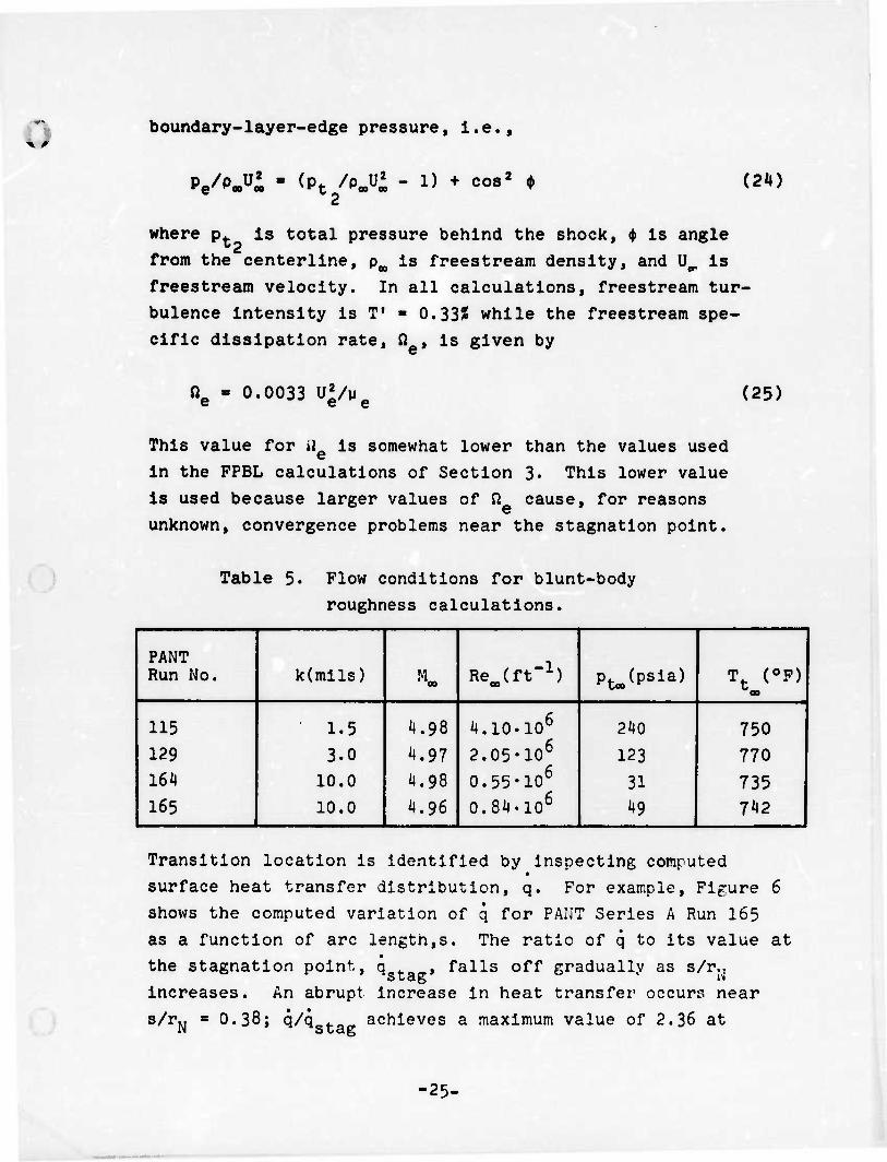
Q boundary-layer-edge pressure. I.e.,

Pe/PX (Pt /P«^ - 1) + cos2 ♦ (2i»)

where p^. Is total pressure behind the shock, $ is angle T'2 from the centerline, p^ is freestream density, and U^. is

freestream velocity. In all calculations, freestream tur-

bulence intensity is T' ■ 0.332 while the freestream spe- cific dissipation rate, Ö , is given by

e 0.0033 U'/Me

This value for »2 is somewhat lower than the values used

in the PPBL calculations of Section 3. This lower value

is used because larger values of ß cause, for reasons

unknown, convergence problems near the stagnation point.

(25)

Table 5. Plow conditions for blunt-body roughness calculations.

PANT Run No. k(mils)

00 Rejft"1) Ptoo(psla) T. (0P)

115 ' 1.5 M8 4.10.106 240 750 129 3.0 ^.97 2.05-10b 123 770 164 10.0 4.98 0.55-106 31 735 165 10.0 4.96 0.84.106 49 742

Transition location is identified by Inspecting computed surface heat transfer distribution, q. For example, Figure 6 shows the computed variation of q for PANT Series A Run 165 as a function of arc length,s. The ratio of q to its value at the stagnation point, q-^-. falls off gradually as s/r., increases. s/r

An abrupt, increase in heat transfer occurs near ly -* 0.38; q/qsta~ achieves a maximum value of 2.36 at

-25-

•

.2 .3 .5 _J

.6

s/r N Figure 6- Keat transfer as a function of arc length

for flow near the stagnation point of a sphere-cone body; PANT Series A Run 165.

-26-

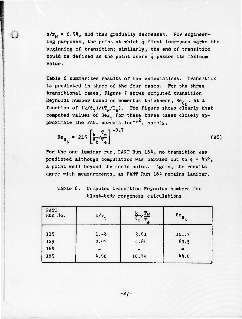
w s/r« » 0.5**, and then gradually decrease*?. For engineer- ing purposes, the point at which q first increases marks the beginning of transition; similarly, the end of transition could be defined as the point where q passes its maximum value.

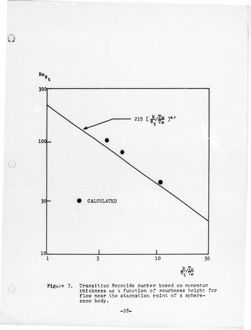
Table 6 summarizes results of the calculations. Transition is predicted in three of the four cases. For the three transitional cases, Figure 7 shows computed transition

as a The figure shows clearly that

three cases closely ap- namely,

-0.7

Reynolds number based on momentum thickness. Re. » function of (k/ei.)/(T /T ). ~ " computed values of Reg for these proximate the PANT correlation1*2,

Re6t - n5 [^y (26)

For the one laminar run, PANT Run 16^1, no transition was

predicted although computation was carried out to $ = ^5°,

a point well beyond the sonic point. Again, the results

agree with measurements, as PANT Run 164 remains laminar.

Table 6. Computed transition Reynolds numbers for

blunt-body roughness calculations

PANT Run No. k/et iL-z^w

et Te Re6 et

115 1.48 3.51 101.7

129 2.0^ 4.84 80.5 164 - - 00

165 4.50 10.74 44.0

-27-

u

Re,

Figure 7. Transition Reynolds nur.ber based on r.or.entun thickness as a function of roughness height for flow near the stagnation point of a sphere- cono body.

-28-

^.1.2 Incipient Transition Calculations

Knowledge of Incipient transition conditions Is Important

In reentry vehicle nosetlp design. Hence, to provide a

further test of the model's ability to predict salient

features of blunt-body transition, a series of calculations

was performed to determine, as a function of roughness

height, k, the minimum freestream unit Reynolds number,

Re^, at which transition occurs. I.e., the Incipient-

transition Re^. Again, computations were for flow near

the stagnation point of a sphere-cone body having a nose

radius, rN, of 2.5 inches. For simplicity, in all cal-

culations freestream Mach number, M , and freestream total

temperature, T. , were 5 and 750oF., respectively; surface

temperature was O.^IT. . The values of T1 and (yß/U2)

were 0.33* and 0.0033.

Four roughness heights were considered, namely, 0.5 mil,

1.5 mils, 3 mils and 10 mils. Table 7 summarizes results,

including momentum thickness at the stagnation point, 9 . ; stag

transition point values of angle, 4)., boundary-layer-edge

Mach number, M , displacement thickness, 6f, and momentum

thickness, et; and the PANT coordinates, (k/et)/(Tw/Te)

and Re0 . 0t

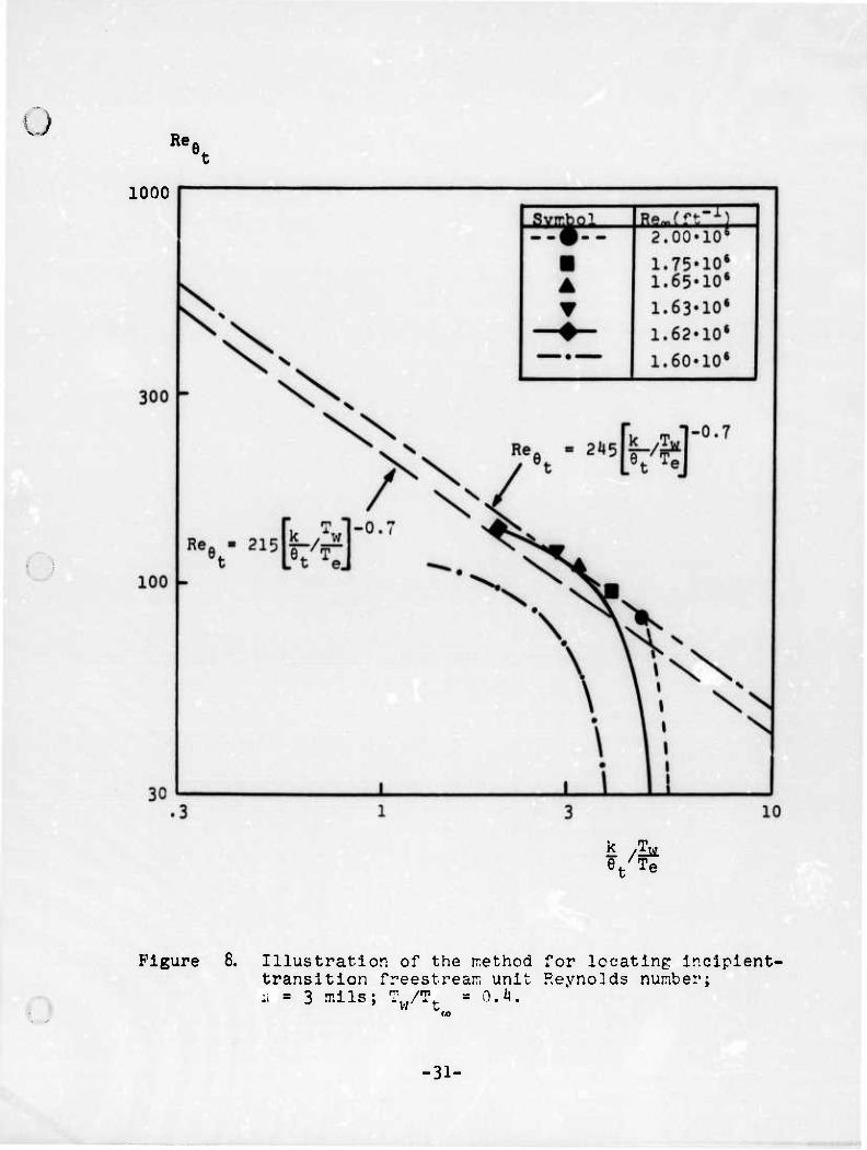
Figure 8 Illustrates calculated behavior for k = 3 nils.

Each symbol denotes transition-point location. As shown,

four of the points lie along the numerical transition cor-

relation (NTC) line defined by

Ree t-^fe^r0,7 ^ which is very close to the PANT correlation [Equation (26)].

-29-

Table 7. Summary of incipient-transition surface-roughness calculations.

k(mils) Re00(ft"1)

i

estaK(mlls) oV) < ö»(mils) et(mils)

k / Tw

V Te

R\

0.5 8.1I2-106 0.66 21.5 0.18 0.39 0.70 1.71 131 6.00-10° 0.78 27.2 0.61 0.52 0.86 1.35 112 4.00.10° 0.96 10.2 0.96 0.81 1.20 0.88 161 3.70-10° 1.00 16.2 1.15 1.05 1.36 0.73 177 3.60-10° 1.01 19.8 1.27 1.20 1.16 0.65 186

3.55-10b

3.50-106 1.02 52.8 1.39 1.35 1.57 0.57 193 1.02 - - - - - eo

1.5 i|.00-106 0.96 23.9 0.53 0.60 1.03 3.15 103 3.00-10° 1.11 36.3 0.85 0.88 1.32 2.18 130 2.70-10° 1.17 51.7 1.31 1.19 1.76 1.56 166 2.65-10b 1.18 - - - - - oo

i 3.0 2.00-106 1.36 27.8 0.63 0.91 1.50 1.61 83 1.75-10° 1.15 35.2 0.82 1.13 1.70 3.88 97 1.65-10b 1.^9 12.6 1.03 1.12 1.92 3.22 111

1.63-10b 1.50 17.3 1.18 1.61 2.09 2.81 120 1.62-10° 1.50 56.1 1.51 2.31 2.56 1.99 137 1.60-10° 1.51 - - - - - 00

10.0 0.80-106 2.15 23.1 0.52 1.31 2.29 10.31 15 0.70-10 2.28 27.8 0.63 1.55 2.53 9.15 19 0.60-10° 2.16 36.0 0.81 1.98 2.91 7.15 58 0.58-10° 2.52 39.6 0.91 2.20 3.12 6.19 62 0.55-10° 2.59 - - - - - 00

'

-30-

o Re.

1000

e/Te

Figure 8. Illustration of the rr.ethod for locating incipient- transition freestream unit Reynolds nunber; ü • 3 mils; T^/T. = O.i».

-31-

The point for Re^ ■ 1.62»10 ft" Is the Incipient case

and lies slightly below the NTC line. The three curves

(referred to as Ree trajectories) are based on computed

values of Reft and (k/e)/(T /T ) up to transition. On the

one hand, for Re^ = 2» 10 ft- the Re^ trajectory Inter-

sects the NTC line, and transition occurs at the inter-

section; on the other hand, when Re^ = 1.60»10 ft" , the

Refl trajectory never intersects the line and no transi-

tion occurs. The incipient case lies between these two

extremes. As shown in Figure 8, the Re« trajectory is

tangent to the NTC line. However, transition does not

occur at the point which would be about midway between

the NTC line and the PANT correlation curve. This be-

havior is consistent with claims that transition loca-

tion and transition onset (i.e., incipient transition

location) are not coincident.

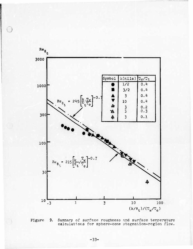
Figure 9 shows that, «'ith the exception of the 0.5-mll

case, all the computed transition-point locations listed

in Table 7 lie along the NTC line. Since corresponding

experimental data also defy correlation, the fact that

0.5-mll numerical data fail to correlate lends further

confidence to the predictions. As with the 3-mil case,

the incipient transition point lies below the NTC line

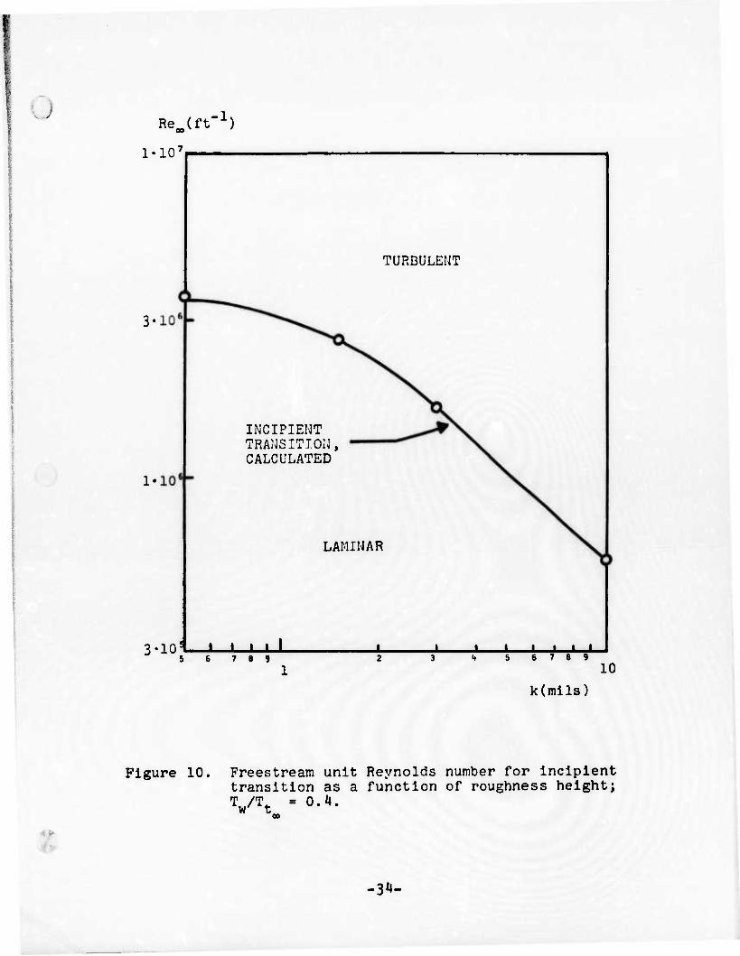
when k = 1.5 mils and k = 10 mils. Figure 10 presents

computed incipient-transition Ite as a function of k;

computed values are very close to measured values .

4.2 SURFACE COOLING

As with surface roughness, effects of surface cooling on

transition for the r,, = 2.5-in., sphere-cone body have

been analyzed in two steps. In the first step, k and Re^

remain constant, and T /T. is varied. In the second step,

-32-

.

Re,

3000

1000

300-

100

30

10

Symbol k(r.lls) Tw/Tt

• 1/2 O.k

■ 3/2 0.4

A T

"A 4^

3 10

3 5 3

0.4 0.4

0.2 0.3 0.1

^

« t e, / ^ X

4 ^

1 1 1 .3 10 100

(k/et)/(Tw/Te)

Figure 9. Summary of surface roughness and surface ter.perature calculations for sphere-cone stagnation-region flow.

-33-

Rejrt-1)

I'lO7

TURBULENT

3*10^

INCIPIENT TRANSITION, CALCULATED

LAMINAR

I I I I J I I—JL 8 9 6 7 8 9

kdnils) 10

Figure 10. Freestream unit Reynolds number for incipient transition as a function of roughness height; w = o.*».

-3^-

with Ite held constant, k Is varied for T./T. = 0.2 00 W too

and 0.8 until Incipient transition conditions are deter-

mined.

For the first set of calculations, the roughness height

Is 3 mils and the corresponding incipient-transition Re^

for T /T. = O.JJ of 1.62» 106 is used. As summarized in W woo

Table 8, surface temperature is varied from 0.1 to 0.8; computed Reg. is shown graphically in Figure 11 as a func- tion of T /Tt . As would be consistent with experimental

W 00

measurements for sphere-cones, surface cooling is predict-

ed to have a destabilizing effect on transition. Figure 9

shows that for T /T. > 0.2, predicted transition location W too """

is close to the PANT correlation line. However, for

T/T*. ■ 0.1, Re0i is about ^OJS lower than the PAHT-cor-

relation value.

In the second set of surface-cooling calculations, Re^

is 1.62'106; k is then varied for T /Tt = 0.2 and 0.8

until incipient-transition conditions have been determined.

Results of the calculations are summarized in Table 8

and Figure 12. An approximate fit to the numerical data

for the incipient-transition roughness height, k. . , is

klnclp ' 10 (VTt. >7/5 f28' '00

with l<i . given in mils.

4.3 BODY GEOMETRY

Effects of body geometry were analyzed by computing in-

cipient-transition conditions for sphere-cones of varying

nose radius. For all of the calculations, the following

conditions have been used:

MM = 5 T* « 13^0° R.

Tw = 500° R. k ' = 3.5 mils } (29)

T' = 0.332 ne = 0.0033 Ue/ye

-35-

J Table 8. Summary of surface-cooling calculations.

VTt. 00 k(mils) bsta*(rnils) tV) «; 6»(mils) et(mils) k /

Tw

Kt 0.10 3.00 1.67 6.6 m.ik 0.12 1.68 17.78 21

0.20 1.62 13.8 0.30 0.03 1.67 8.90 ! 11

0.30 1.56 23.1 0.52 0.51 1.66 5.69 1 66 ' | 0.38 1.51 36.6 0.86 1.11 1.81 3.80 97

0.il5 1.118 - - - - - 00 !

0.80 1.30 - - - - - 00

0.20 2.00 1.62 20.k 0.h5 0.06 1.70 5.65 60

1.50 28.1 0.63 0.10 1.80 3.86 82

1.00 50.3 1.29 0.15 2.11 1.51 138

0.98 53.6 1.12 0.55 2.63 1.33 116

0.97 56.1 1.53 0.65 2.81 1.18 152 j 1 0.95 - - - - - 00 1

0.80 10.00 1.30 27.0 0.61 2.55 1.10 8.29 62

8.00 36.9 0.86 2.99 1.51 5.76 82

7.50 52.3 1.37 1.19 1.86 3.6? 105

7.^9 - - - - - 00

Boundary-layer-edge pressure is again given by the modified

Newtonian distribution [Equation (21)]. Three nose radii are

considered, namely, 0.75 in., 2.5 in. and 3-5 in.; Table 9

summarizes the calculations. As shown in Figure 13, rN has

only a slight effect on the Incipient-transition Re^, with

increasing nose radius yielding lower values for Re^. This 31 trend is consistent with recent measurements , thus providing

another test of the theory. The numerical data are closely

-36-

L)

Tw/T

100

Re(

Figure 11. Effect of surface temperature on transition for constant freostrearr. unit Reynolds number, Re_ = 1.62'106 cer foot.

-37-

u

1.0 9

7

6 L.

5 -

LAMINAR

k = 10(TW/Tt )

TURBULENT

o.iLa 8 9

J 1 1 | | | 6 7 8 9 10

k(mils)

Figure 12. Minimum roughness height for incipient transition as a function of surface temperature; Re^ = 1.62*10s

per foot.

-33-

Table 9. Sununary of nose radius calculati< Dns

rN(ln) Rejft"1) Wmlls) k(0) k 1

öj^mils) 1

et(inils) k ^w ReA et J 0.75 2.00-1O6 0.74 24.75 0.55 0.42 0.80 11.05 42.4 1

1.50-1O6 0.85 Uo.34 0.97 0.69 1.08 7.32 57.5

I.HS-IO6 0.86 43.09 1.07 O.76 1.13 6.75 60.7

l.kl'106 0.86 46.20 1.15 0.82 1.18 6.29 63.3 1.46-106 0.86 - - - - - so

2.50 l.i*0-106 1.61 33.56 0.78 1.07 1.87 4.47 85.6 1 1.30'106 1.67 41.81 1.01 1.38 2.14 3.64 99.9 1 1.28-106 1.69 47.86 1.20 1.69 2.38 3.06 110.8

1.27-10b 1.69 - - - - - 00 1

3.50 2.00-106 1.60 19.25 0.42 0.82 1.67 5.43 71.9

1.50-10b 1.85 27.70 0.62 1.09 2.04 4.29 88.2

1.40-106 1.91 30.64 0.70 1.20 2.16 3.95 93.7

1.35-106 f l 1.9^ 33.00 0.76 1.21 2.24 3.75 98.0

1.32-10b 1.97 34.96 0.81 1.35 2.32 3.58 102.1

1.30-106 i 1.98 35.75 0.83 1.39 2.35 3.50 103.3 1.27-10° 2.00 j 37.91 0.89 1.48 2.44 3.32 107.6

1.23-106 2.04 1 42.62 1.03 1.72 2.64 2.94 116.9 1.21-106 \ 2.05 47.93 1.20 2.05 2.89 2.52 127.4

1.20'10b 2.06 ! - - - - 00 I

-39-

.; lO"6 Re^Cft'1)

1.6

l.H

1.0

1.2

y Re -1.113-lO6!--1^ 00 N

CALCULATED

rN(in)

Figure 13. Dependence of incipient freestream unit Reynolds

number on nose radius for sphere-cones; k*3.5 mils,

■ 0.373. T /T. w t

-JlO-

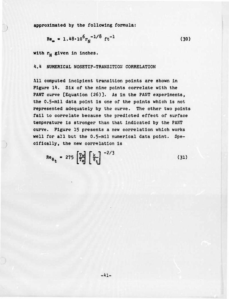
approximated by the following formula:

Re^ - l.i*8.106rN"1/8 ft"1 (30)

with r« given In Inches.

4.1i NUMERICAL NOSETIP-TRANSITION CORRELATION

All computed Incipient transition points are shown In

Figure 14. Six of the nine points correlate with the

PANT curve [Equation (26)]. As in the PANT experiments,

the 0.5-mil data point is one of the points which is not

represented adequately by the curve. The other two points

fall to correlate because the predicted effect of surface

temperature is stronger than that indicated by the PANT

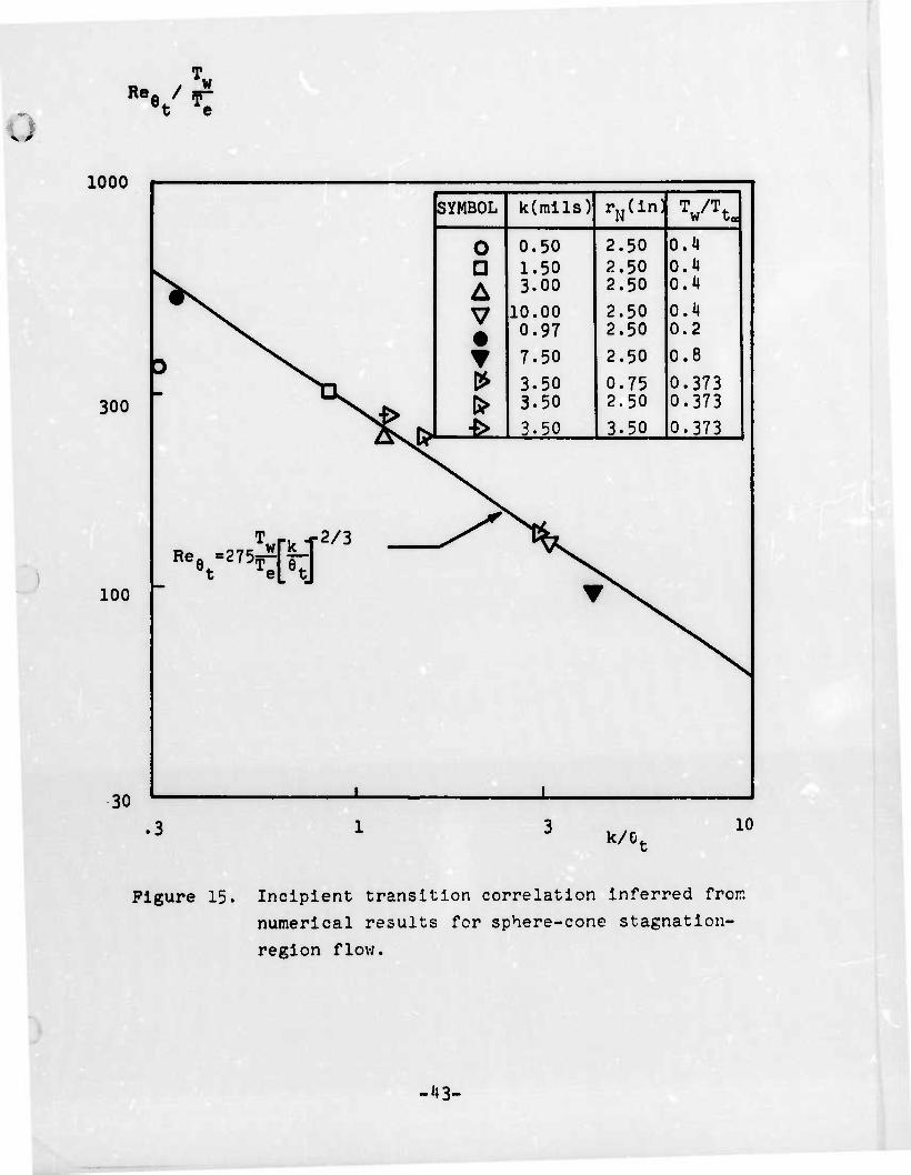
curve. Figure 15 presents a new correlation which works

well for all but the 0.5-mil numerical data point. Spe-

cifically, the new correlation is

Ree . - - m [k] ■2/3

-m-

Re e. ' 1000

300

100

30

SYMBOL k(rr.ils) r„(ln) VH* 0 0.5 2.5 Ö.Ü

1.5 2.5 0.4 3.0 2.5 O.i*

^ 10.0 2.5 0.4 • 0.97 2.5 0.2 ▼ 7.5 2.5 0.8

> 3.5 0.75 0.373

> 3.5 2.5 0.373 ■> 3.5 3.5 0.373

ReQ =215

.3 10

T _k_/w et Te

Figure 14. Comparison of computed Incipient transition

points with the PANT •■.■orrelation.

-4?-

Q «s / 5;

1000

300

100

30

.3

1

SYMBOL k(inils) rN(ln; W to

0 a

0.50 1.50 3.00

2.50 2.50 2.50

0.4 0.4

V #

10.00 0.97

2.50 2.50

0.H 0.2

1 \s.

s

7.50

3-50 3.50

2.50

0.75 2.50

0.8

0.373 0.373

*> 3.50 3.50 0.373

Vk T2/3 Refl =275^ f- 8t Mt

^

▼ N.

i i

k/G, 10

Figure 15. Incipient transition correlation inferred fror.

numerical results for sphere-cone stagnation-

region flow.

-43-

5.0 DISCUSSION

Results presented in Sections 3 and 'I show that accurate

transition predictions can be made with the Saffman-

turbulence-model equations, provided low-Reynolds-number

effects are taken into account (Section 2). V/ith only

one adjustable parameter, namely R , the model yields ac-

curate transition predictions for incompressible boundary

layers and for stagnation-region flows. The effects of

freestream turbulence, surface roughness, and suction on

incompressible FPBL transition are well represented by

the model; surface-roughness, surface-cooling, and body-

geometry effects on blunt-body transition also have been

predicted accurately.

The fact that the model works equally well for constant-

pressure boundary layers and for stagnation-region flows

is a key feature of the technique. That is, although

further study will be needed to establish the model's

range of applicability, the fact that the initial data

base includes these two classes of flows provides hope

that a universally applicable transition-prediction

method has been developed.

Specific areas needing further model development and

validation Include effects on transition of freestream

turbulence, compressibility and pressure gradient. As

shown in Section 2, freestream-turbulence scale has a

large effect on FPBL transition. While some effect is

expected on physical grounds, no attempt has been made

to determine whether or not the predicted effect is even

qualitatively correct. Sensitivity of blunt-body tran-

sition to both freestream-turbulence intensity and scale

should also be determined. The predicted role of free-

stream turbulence in rough-wall transition requires

-HH-

further elucidation. Compressibility effects should be

analyzed In detail for FPBL flows for which extensive

experimental data are available. Surface cooling and

freestream Mach number are easily represented with the

model and should be analyzed to help test validity of

the predicted stronger-than-measured effect of surface

cooling on blunt-body transition. While pressure-gradient

effects have been addressed indirectly by analyzing FPBL

flow and the blunt-body geometric configurations, more-

direct tests of the model are needed. Again, extensive

experimental data exist for the effect of pressure gra-

dient on boundary-layer transition, so that definitive

tests of the model can be easily made.

In conclusion, the computations in Section '; exemplify

the turbulence-model-transition-prediction method's poten-

tial value to the reentry-vehicle-nosetip-design engineer.

The EDDYBL computer code has been used in Section 4 as a

"numerical wind tunnel" in that PANT Series A experiments

have been simulated including a wider range of surface

temperatures than could be covered in the physical tunnel.

Many of the predicted results agree with measured flow

properties. In particular, measured and computed effects

of surface temperature on sphere-cone transition are in

close agreement for the range of temperatures in the PANT

experiments; however, computations at lower temperatures

than those which could be considered in the PANT experi-

ments indicate that surface cooling has a stronger effect

than that inferred from the experimental data. This in-

dicates an area in which further measurements are needed.

Additionally, this exemplifies the fact that arbitrary

flow conditions can be simulated in the numerical wind

tunnel while the physical wind tunnel often is limited.

Hence, the numerical wind tunnel can be used to test and

verify the transition-prediction method for both ground-

test and flight-test data and, as the ultimate goal, can

be used to predict nosetip transition under real flight

conditions.

-H5-

APPENDIX

THE EDDYBL COMPUTER CODE

Computations in this study were performed with the EDDYBL

computer code. This code is based on a boundary-layer 21 program developed at the NASA Langley Research Center ;

the Saffman turbulence equations were incorporated in the 30 code in a DCW Industries research project . The integra-

tion method embodied in EDDYBL is similar to the implicit 31 Flugge-Lotz and Blottner technique in which the momentum

and energy equations are coupled. In adding the turbulence model to the code, the two nonlinear diffusion equations

(4, 5) are solved in a coupled manner analogous to that

used for the momentum and energy equations in the origi-

nal version of the code. Since all four equations are

not solved simultaneously, an iterative procedure is needed to obtain an accurate solution. As part of this

study, a more efficient iterative procedure than had been

used previously was developed.

The new iterative scheme (Figure Al) takes advantage of

the special nature of transition-prediction calculations.

Specifically, note that for laminar flow the momentum and

energy equations are not coupled to the turbulence-density

equations. Kence, with no sacrifice of accuracy, the

momentum and energy equations can be solved non.'teratlvely

at each station on laminar regions. Since the turbulence density equations do require iteration when the flow is

laminar, eliminating the momentum and energy equations

from the iterative loop significantly reduces computing

time. In specifying when all four equations must be solvoH Itcratlvely, the criterion is that the maximum

value (with respect to distance from the boundary) of the

kinematic eddy viscosity, e, exceed 5^ of the kinematic

-46-

Specify

Initial

Profiles

I Proceed to

Next Station r~ Integrate mean

Momentum and

Energy Equations

I Integrate

Turbulence

Density

Equations

Yes

Yes

Figure Al. Schematic of iterative method used in the EDDYBL code.

-H7-

) molecular viscosity, v.

Experience with EDDYBL shows that the turbulent energy converges more slowly than the other field variables. Two of the most sensitive turbulent-energy values are the peak turbulent energy and the value at the mesh point nearest the surface. These two quantities are therefore monitored to determine when convergence is attained; convergence is defined to occur when these two quantities change by less than 1% between successive iterations. Two or three iterations appear to be suitable on both laminar and turbulent regions, while seven or eight iterations typica'.ly are required through transition.

-H8-

REFERENCES

1. Jackson, M.D. and Baker, D.L., "PANT Series B Wind- Tunnel Test Data Report," Aerotherm Project No. 7042, Aerotherm Acurex Corp., Mountain View, California (1972).

2. Jackson, M.D., Baker, D.L. and Powars, CA., "PANT Series A Wind-Tunnel Test Data Report," Aerotherm Pro- ject No. 7042, Aerotherm Acurex Corp., Mountain View, California (1972).

3. Demetrlades, A. and Laderman, A.J., "Final Progress Report - Advanced Penetration Problems Program," SAMSO Report No. 73-397, Space and Missile Systems Organiza- tion, Los Angeles, California (1971»).

4. Laderman, A.J., "Effect of Mass Addition and Angle-of- Attack on the Hypersonic Boundary Layer Turbulence Over a Slender Come," Phllco-Ford Report No. U-6047, Philco- Ford Corp., Aeronutronic Division, Newport Beach, California (1973).

5. Schubauer, G.B. and Skramstad, H.K., "Laminar Boundary Layer Oscillations and Stability of Laminar Flow," Journal of Aero. Sei. 14, p. 69 (19^7).

6. Liepmann, H.W. and Flla, G.H., "Investigations of Ef- fect of Surface Temperature and Single Roughness Ele- ments on Boundary Layer Transition,"NACA 890 (19^7).

7. Feindt, E.G., "Untersuchungen über die Abhängigkeit des Umschlages laminar-turbulent von der Oberflächen- rauhigkeit und der Druckverteilung," Thesis Braun- schweig 1956; Jahrbuch 1956 der Schiffbautech nischen Gesellschaft 50, pp 180-203 (1957).

8. van Driest, E.R. and Blumer, C.B., "Boundary Layer Transition: Free-Stream Turbulence and Pressure Gradient Effects," AIAA Journal, Vol. 1, pp 1303-1306 (1963).

9. Personal communication with S. Orszag, Flow Research, Inc., July 1974.

10. Schllchting, K., Boundary Layer Theory, Fourth Edition, McGraw Hill, Hew York (1962).

11. Mack, L.H., "On the Application of Linear Stability Theory to the Problem of Supersonic Boundary-Layer Transition," AIAA Paper 74-134 (1974).

-49-

12. Smith, A.M.O. and Gamberonl, N., "Transition, Pressure Gradient, and Stability Theory," Report ES 26388, Douglas Aircraft Co., Inc., El Segundo, California (1956).

13. Kaplan, R.E., "Generation of Turbulence-Transition," Unpublished notes. University of Southern California (197M.

14. Donaldson, C.duP., "A Computer Study of an Analytical Model of Boundary Layer Transition," AIAA Paper 68-38 (1968).

15. Jones, W.P. and Launder, B.E., "Calculation of Low Reynolds Number Phenomena with a Two-Equation Model of Turbulence," Int. J. Heat and Mass Trans. 16, pp 1119-1129 (1973).

16. Wllcox, D.C., "Turbulence Model Calculation of Raylelgh Shear Flow," DCW Industries Report DCW-R-IJC-Ol, DCW Industries, Sherman Oaks, California (197^).

17. Saffman, P.G., "A Model for Inhomogeneous Turbulent Flow," Proc. Roy. Soc. Lond. A317, pp ^17-^33 (1970).

18. Wllcox, D.C. and Alber, I.E., "A Turbulence Model for High Speed Flows," Proceedings of the 1972 Heat Trans- fer and Fluid Mechanics Institute, Stanford Univ. Press, pp 231-252 (1972).

19. Saffman, P.G. and Wllcox, D.C, "Turbulence-Model Predictions for Turbulent Boundary Layers," AIAA Journal, Vol. 12, Mo. 4, pp 5^1-5^6 (197^).

20. Favre, A.J., "The Equations of Compressible Turbulent Gases," Annual Sumr.ary Report No. 1, Institute de Mechanique Statistique de la Turbulence (1965).

21. Harris, J.E., "Numerical Solution of the Equations for Compressible Laminar, Transitional, and Turbulent Boundary Layers and Comrarisons with Experimental Data," NASA TR R-368 (1971).

22. Rotta, J.C., "Statistiche Theorie Nichthomogener Turbulenz," Zeitschrift für Physik, Vol. 131, pp 51-77 (1951).

23. Dryden, H.L., Aerodynamics and Jet Frorulslon, V, University Press, Princeton, N.J. (1959)•

-50-

2i|. Hall, A.A. and Hislop, G.S., "Experiments on the Transition of the Laminar Boundary Layer on a Plat Plate," ARC R&M 1813 (1938).

25. Baliey-Wrlght data as tabulated by Dryden In Refe- rence 23.

26. Spangler, J.G. and Wells, C.S.,Jr., "Laminar-Boundary- Layer Oscillation and Transition on a Plat Plate," NACA 909 (19^8).

27. Simpson, R.L., Moffat, R.J. and Kays, W.M., "The Turbulent Boundary Layer on a Porous Plate: An Experimental study of the Fluid Dynamics with Suc- tion and Injection," Univ. Stanford Thermosciences Div. Rej. rt HMT-2, Stanford University (1972).

28. Pfenninger, W. and Bacon, J.W., "Investigation of Methods for Re-Establishment of a Laminar Boundary Layer from Turbulent Flow," Northrop Report :.T0R 65-^8, Northrop Corp., Hawthorne, Calif. (1965).

29. Schlichting, H., Boundary Layer Theory, Fourth Edition, McGraw-Hill, New York, p 426 (I960).

30. Wilcox, D.C., "Turbulence-Model Transition Predictions for Compressible and Incompressible Flat-Plate Boun- dary Layers with Suction," DCW Industries Technical Note DCW-TN-01-01 (1971).

31. Flugge-Lotz, I. and Blottner, F.G., "Computation of the Compressible Laminar Boundary-Layer Flow Includ- ing Displacement-Thickness Interaction Using Finite- Difference Methods," AFOSR 2206 (1962).

-51-