distribute student manual or duplicate€¦ · microsoft® office excel® 2010: part 2 (second...

Microsoft® OfficeExcel® 2010: Part2 (Second Edition)

STUDENT MANUAL

Do Not D

uplicate

or Dist

ribute

Microsoft® OfficeExcel® 2010: Part

2 (SecondEdition)

Do Not D

uplicate

or Dist

ribute

Microsoft® Office Excel® 2010: Part 2(Second Edition)Part Number: 091019Course Edition: 1.0

AcknowledgementsPROJECT TEAM

Author Media Designer Content Editor

Tim Barnosky Alex Tong Catherine M. Albano

NoticesDISCLAIMERWhile Logical Operations, Inc. takes care to ensure the accuracy and quality of these materials, we cannot guarantee theiraccuracy, and all materials are provided without any warranty whatsoever, including, but not limited to, the implied warranties ofmerchantability or fitness for a particular purpose. The name used in the data files for this course is that of a fictitious company. Anyresemblance to current or future companies is purely coincidental. We do not believe we have used anyone's name in creating thiscourse, but if we have, please notify us and we will change the name in the next revision of the course. Logical Operations is anindependent provider of integrated training solutions for individuals, businesses, educational institutions, and government agencies.Use of screenshots, photographs of another entity's products, or another entity's product name or service in this book is for editorialpurposes only. No such use should be construed to imply sponsorship or endorsement of the book by, nor any affiliation of suchentity with Logical Operations. This courseware may contain links to sites on the internet that are owned and operated by thirdparties (the "External Sites"). Logical Operations is not responsible for the availability of, or the content located on or through, anyExternal Site. Please contact Logical Operations if you have any concerns regarding such links or External Sites.

TRADEMARK NOTICESLogical Operations and the Logical Operations logo are trademarks of Logical Operations, Inc. and its affiliates.Microsoft® and Excel® are registered trademarks of Microsoft Corporation in the U.S. and other countries. The other Microsoftproducts and services discussed or described may be trademarks or registered trademarks of Microsoft Corporation. All otherproduct and service names used may be common law or registered trademarks of their respective proprietors.Copyright © 2014 Logical Operations, Inc. All rights reserved. Screenshots used for illustrative purposes are the property of thesoftware proprietor. This publication, or any part thereof, may not be reproduced or transmitted in any form or by any means,electronic or mechanical, including photocopying, recording, storage in an information retrieval system, or otherwise, withoutexpress written permission of Logical Operations, 3535 Winton Place, Rochester, NY 14623, 1-800-456-4677 in the United Statesand Canada, 1-585-350-7000 in all other countries. Logical Operations’ World Wide Web site is located atwww.logicaloperations.com.This book conveys no rights in the software or other products about which it was written; all use or licensing of such software orother products is the responsibility of the user according to terms and conditions of the owner. Do not make illegal copies of booksor software. If you believe that this book, related materials, or any other Logical Operations materials are being reproduced ortransmitted without permission, please call 1-800-456-4677 in the United States and Canada, 1-585-350-7000 in all other countries.Do N

ot Duplic

ate or D

istrib

ute

Microsoft® Office Excel®2010: Part 2 (SecondEdition)

Lesson 1: Customizing the Excel Environment................ 1Topic A: Configure Excel Options................................................... 2Topic B: Customize the Ribbon and the Quick Access Toolbar...... 10Topic C: Enable Excel Add-Ins......................................................18

Lesson 2: Creating Advanced Formulas.........................23Topic A: Use Range Names in Formulas........................................ 24Topic B: Use Specialized Functions............................................... 34Topic C: Use Array Formulas........................................................ 43

Lesson 3: Analyzing Data with Functions andConditional Formatting.......................................... 53Topic A: Analyze Data by Using Text and Logical Functions..........54Topic B: Apply Advanced Conditional Formatting..........................68

Lesson 4: Organizing and Analyzing Datasets andTables....................................................................79Topic A: Create and Modify Tables............................................... 80

Do Not D

uplicate

or Dist

ribute

Topic B: Sort Data...................................................................................87Topic C: Filter Data.................................................................................95Topic D: Use SUBTOTAL and Database Functions..................................105

Lesson 5: Visualizing Data with Basic Charts.......................121Topic A: Create Charts......................................................................... 122Topic B: Modify and Format Charts.......................................................128

Lesson 6: Analyzing Data with PivotTables, Slicers, andPivotCharts.................................................................. 137Topic A: Create a PivotTable.................................................................138Topic B: Analyze PivotTable Data..........................................................144Topic C: Present Data with PivotCharts................................................. 157Topic D: Filter Data by Using Slicers..................................................... 162

Appendix A: Financial Functions......................................................... 173

Appendix B: Date and Time Functions.................................................177

Appendix C: Working with Graphical Objects...................................... 181Topic A: Insert Graphical Objects..........................................................182Topic B: Modify Graphical Objects........................................................ 187Topic C: Work with SmartArt.................................................................191

Appendix D: Microsoft Office Excel 2010 Exam 77-882......................197

Appendix E: Microsoft Office Excel 2010 Expert Exam 77–888............203

Lesson Labs............................................................................................ 207

Solutions................................................................................................ 217

Glossary............................................................................................. 221Index..................................................................................................225

| Microsoft® Office Excel® 2010: Part 2 (Second Edition) |

Do Not D

uplicate

or Dist

ribute

About This Course

Whether you need to crunch numbers for sales, inventory, information technology, humanresources, or other organizational purposes and departments, the ability to get the rightinformation to the right people at the right time can create a powerful competitiveadvantage. After all, the world runs on data more than ever before and that's a trend notlikely to change, or even slow down, any time soon. But with so much data available andbeing created on a nearly constant basis, the ability to make sense of that data becomesmore critical and challenging with every passing day. You already know how to get Excel toperform simple calculations and how to modify your workbooks and worksheets to makethem easier to read, interpret, and present to others. But Excel is capable of doing so muchmore. In order to gain a truly competitive edge, you need to be able to extract actionableorganizational intelligence from your raw data. In other words, when you have questionsabout your data, you need to know how to get Excel to provide the answers for you. Andthat's exactly what this course aims to help you do.This course builds upon the foundational knowledge presented in the Microsoft® Office Excel®2010: Part 1 (Second Edition) course and will help start you down the road to creatingadvanced workbooks and worksheets that can help deepen your organizational intelligence.The ability to analyze massive amounts of data, extract actionable intelligence from it, andpresent that information to decision makers is the cornerstone of driving a successfulorganization that is able to compete at a high level.This course covers Microsoft Office Specialist exam objectives to help students prepare forthe Excel 2010 Exam and the Excel 2010 Expert Exam.

Course DescriptionTarget StudentThis course is designed for students who already have foundational knowledge and skills inExcel 2010 and who wish to begin taking advantage of some of the higher-levelfunctionality in Excel to analyze and present data.

Course PrerequisitesTo ensure success, students should have completed Logical Operations’ Microsoft® OfficeExcel® 2010: Part 1 (Second Edition) or have the equivalent knowledge and experience.

Course ObjectivesUpon successful completion of this course, you will be able to leverage the power of dataanalysis and presentation in order to make informed, intelligent organizational decisions.You will:• Customize the Excel environment.

Do Not D

uplicate

or Dist

ribute

• Create advanced formulas.• Analyze data by using functions and conditional formatting.• Organize and analyze datasets and tables.• Visualize data by using basic charts.• Analyze data by using PivotTables, slicers, and PivotCharts.

The LogicalCHOICE Home ScreenThe LogicalCHOICE Home screen is your entry point to the LogicalCHOICE learning experience,of which this course manual is only one part. Visit the LogicalCHOICE Course screen both duringand after class to make use of the world of support and instructional resources that make up theLogicalCHOICE experience.Log-on and access information for your LogicalCHOICE environment will be provided with yourclass experience. On the LogicalCHOICE Home screen, you can access the LogicalCHOICECourse screens for your specific courses.Each LogicalCHOICE Course screen will give you access to the following resources:• eBook: an interactive electronic version of the printed book for your course.• LearnTOs: brief animated components that enhance and extend the classroom learning

experience.Depending on the nature of your course and the choices of your learning provider, theLogicalCHOICE Course screen may also include access to elements such as:• The interactive eBook.• Social media resources that enable you to collaborate with others in the learning community

using professional communications sites such as LinkedIn or microblogging tools such asTwitter.

• Checklists with useful post-class reference information.• Any course files you will download.• The course assessment.• Notices from the LogicalCHOICE administrator.• Virtual labs, for remote access to the technical environment for your course.• Your personal whiteboard for sketches and notes.• Newsletters and other communications from your learning provider.• Mentoring services.• A link to the website of your training provider.• The LogicalCHOICE store.Visit your LogicalCHOICE Home screen often to connect, communicate, and extend your learningexperience!

How to Use This BookAs You LearnThis book is divided into lessons and topics, covering a subject or a set of related subjects. In mostcases, lessons are arranged in order of increasing proficiency.The results-oriented topics include relevant and supporting information you need to master thecontent. Each topic has various types of activities designed to enable you to practice the guidelinesand procedures as well as to solidify your understanding of the informational material presented inthe course. Procedures and guidelines are presented in a concise fashion along with activities anddiscussions. Information is provided for reference and reflection in such a way as to facilitateunderstanding and practice.Data files for various activities as well as other supporting files for the course are available bydownload from the LogicalCHOICE Course screen. In addition to sample data for the course


| About This Course |

Do Not D

uplicate

or Dist

ribute

exercises, the course files may contain media components to enhance your learning and additionalreference materials for use both during and after the course.At the back of the book, you will find a glossary of the definitions of the terms and concepts usedthroughout the course. You will also find an index to assist in locating information within theinstructional components of the book.

As You ReviewAny method of instruction is only as effective as the time and effort you, the student, are willing toinvest in it. In addition, some of the information that you learn in class may not be important to youimmediately, but it may become important later. For this reason, we encourage you to spend sometime reviewing the content of the course after your time in the classroom.

As a ReferenceThe organization and layout of this book make it an easy-to-use resource for future reference.Taking advantage of the glossary, index, and table of contents, you can use this book as a firstsource of definitions, background information, and summaries.

Course IconsWatch throughout the material for these visual cues:

Icon Description

A Note provides additional information, guidance, or hints about a topic or task.

A Caution helps make you aware of places where you need to be particularly carefulwith your actions, settings, or decisions so that you can be sure to get the desiredresults of an activity or task.

LearnTO notes show you where an associated LearnTO is particularly relevant tothe content. Access LearnTOs from your LogicalCHOICE Course screen.

Checklists provide job aids you can use after class as a reference to performingskills back on the job. Access checklists from your LogicalCHOICE Course screen.

Social notes remind you to check your LogicalCHOICE Course screen foropportunities to interact with the LogicalCHOICE community using social media.

Notes Pages are intentionally left blank for you to write on.


| About This Course |

Do Not D

uplicate

or Dist

ribute

Do Not D

uplicate

or Dist

ribute

Customizing the ExcelEnvironmentLesson Time: 45 minutes

Lesson ObjectivesIn this lesson, you will customize the Excel environment. You will:

• Configure Excel options.

• Customize the ribbon and the Quick Access Toolbar.• Enable Excel add-ins.

Lesson IntroductionAs you are already familiar with Excel 2010, you are, no doubt, able to navigate your wayaround the Excel environment and locate the basic commands you frequently use. But noteveryone uses Excel in the same way and, depending on what you use Excel for, you mayuse whole sets of commands regularly that other users barely touch. Wouldn't it be nice ifyou could configure the Excel environment to better suit your regular daily work flow? Orperhaps there are default settings within Excel that don't quite mesh with your needs, suchas the default number of worksheets in a workbook or the default location for saving files.In addition, there are a number of supplemental applications and features that not everyoneuses, so they don't automatically come activated. What if you're one of the users who has aneed for these features?Like the other Microsoft Office 2010 applications, Excel 2010 provides you with a widevariety of options when it comes to customizing your Excel experience. Knowing where tofind these options and what they do will not only save you time and effort, but it can alsohelp you craft an Excel environment that meshes with your preferred work flow.

1

Do Not D

uplicate

or Dist

ribute

TOPIC AConfigure Excel OptionsSome of Excel's default settings and options have an easily observable effect on your overall Excelexperience. Consider, for example, the number of worksheets included in a new workbook. Othersettings, such as where Excel automatically saves files, are less obvious. Global system settings inExcel have a direct impact on your experience as a user. As so many people use Excel, and for vastlydifferent purposes, it makes sense that configuring and changing these options and settings can havea significant impact on how efficiently Excel works for you.Excel 2010 provides you with a vast array of options for tweaking the behind the scenes behavior ofthe application to suit nearly any organizational or specific user need. Knowing where to find theseoptions, and what each of them do, will make it easy for you to quickly adjust Excel's defaultbehavior whenever the need arises. This means that when you need to react to changes in your workenvironment, you can quickly configure Excel to work the way you need it to, when you need it.

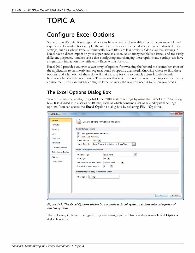
The Excel Options Dialog BoxYou can adjust and configure global Excel 2010 system settings by using the Excel Options dialogbox. It is divided into a series of 10 tabs, each of which contains a set of related system settingsoptions. You can access the Excel Options dialog box by selecting File→Options.

Figure 1-1: The Excel Options dialog box organizes Excel system settings into categories ofrelated options.

The following table lists the types of system settings you will find on the various Excel Optionsdialog box tabs.

2 | Microsoft® Office Excel® 2010: Part 2 (Second Edition)

Lesson 1: Customizing the Excel Environment | Topic A

Consider beginning thislesson with a generaldiscussion ofcustomization. Exceloffers a variety ofoptions within theapplication and there area number of plug-insavailable to customizethe environment. Asover-customizing canquickly becomeoverwhelming, remindstudents they canalways reset Excel to thedefault settings and startover.The Excel OptionsDialog Box

This topic is meant toserve as an overview ofthe options available inExcel 2010; it is notmeant to be acomprehensiveexploration of all ofthem. Consider orientingthe students, from a highlevel, to where they canlocate the variousoptions and settings, butnot covering each ingreat detail. Studentswill practice some of themore commonlyadjusted option settingsduring the activity.

Do Not D

uplicate

or Dist

ribute

Excel Options Dialog BoxTab

Contains Options For

General Adjusting the display of certain on-screen elements and toolbars,configuring the default settings for new workbooks, and personalizingExcel for a particular user.

Formulas Configuring formula and error checking settings.

Proofing Configuring AutoCorrect settings, configuring spelling check settings,and selecting the desired dictionary and language to use for proofingfeatures.

Save Selecting how often and to which directory Excel automatically savesworkbook files, configuring offline editing settings, and preservingvisual aspects of workbooks when opening workbook files in previousversions of Excel.

Language Selecting the desired language for Excel editing features, for worksheetcontent, and for ScreenTips.

Advanced Adjusting settings that directly affect many common Excel tasks.

Customize Ribbon Customizing the tabs, groups, and commands on the ribbon.

Quick Access Toolbar Customizing the Quick Access Toolbar.Add-Ins Installing, activating, and deactivating supplemental Excel features and

functionality.

Trust Center Configuring privacy and security settings that affect all Office 2010applications.

General OptionsThe General tab in the Excel Options dialog box contains settings that affect some commonExcel functionality.

General Tab Section Contains Options For

User Interface options Managing the display of the Mini Toolbar, the Live Preview feature,and ScreenTips, and for selecting the color scheme for the Excelapplication window.

When creating newworkbooks

Managing default workbook settings, such as the font and font size,the view to which workbooks open, and the number of worksheets ina new blank workbook.

Personalize your copyof Microsoft Office

Modifying the default user name for all Office 2010 applications. Thisis the name that will be displayed as the author in Office file propertiesand in comments you add to documents.

Formulas OptionsThe Formulas tab in the Excel Options dialog box contains settings that affect how Excel workswith and displays formulas and functions, and how error checking features behave.

Formulas Tab Section Contains Options For

Calculation options Configuring how Excel executes calculations in functions andformulas.

Microsoft® Office Excel® 2010: Part 2 (Second Edition) | 3


The OV slide for theExcel Options dialog boxdisplays the General tab.

Formulas OptionsDo Not D

uplicate

or Dist

ribute

Formulas Tab Section Contains Options ForWorking with formulas Toggling formula features on or off.

Error Checking Toggling automatic error checking on or off, and changing the displayof discovered errors.

Error checking rules Toggling particular error-checking rules on or off.

Proofing OptionsThe Proofing tab in the Excel Options dialog box contains settings that affect how Excelperforms AutoCorrect and spelling check functions.

Proofing Tab Section Description

AutoCorrect options Displays the AutoCorrect Options button, which opens theAutoCorrect dialog box.

When correctingspelling in MicrosoftOffice programs

Contains options for managing how Excel, and other Officeapplications, check for misspellings, for selecting the dictionary againstwhich Excel checks word spellings, and for configuring particularlanguage-specific options.

The AutoCorrect Dialog BoxThe AutoCorrect dialog box contains options settings for managing how Excel automaticallycorrects spelling and other data entry issues as you type. It is divided into a series of four tabs thatcontain related settings options.

Figure 1-2: Use the AutoCorrect dialog box to configure how Excel corrects commonmisspellings.



Proofing Options

The AutoCorrect DialogBox

Do Not D

uplicate

or Dist

ribute

AutoCorrect Dialog Box Tab Contains Options For

AutoCorrect Toggling specific AutoCorrect functionality on and off, such aswhether or not Excel automatically capitalizes the first word ofa sentence if you forget to. From here you can also manage howExcel automatically corrects common typing errors such asreplacing "teh" with "the."

AutoFormat As You Type Toggling particular AutoFormatting options on or off, such aswhether or not Excel automatically formats URLs as hyperlinks.

Actions Enabling or disabling additional automatic actions in contextmenus.

Math AutoCorrect Managing how Excel automatically enters mathematical symbolsbased on keyboard input. For example, by default, if you type\pi, Excel replaces the text with the mathematical symbol π.

Save OptionsThe Save tab in the Excel Options dialog box contains settings that affect how and to whichdirectory Excel saves workbook files.

Save Tab Section Contains Options For

Save workbooks Selecting the default file format that Excel saves workbooks in,for determining how often Excel automatically saves unsavedworkbooks and for selecting the default directories for savingworkbooks and for the AutoRecover feature.

AutoRecover Exceptions for Enabling or disabling the AutoRecover feature for particularworkbooks.

Offline editing options fordocument management serverfiles

Selecting where Excel saves draft copies of workbook files thatyou check out of a Microsoft SharePoint site.

Preserve visual appearance ofthe workbook

Selecting or modifying the color palette that Excel will use whenopening a workbook in a previous version of Excel.

Language OptionsThe Language tab in the Excel Options dialog box contains settings that affect which languagesand dictionaries Excel references for a variety of purposes.

Language Tab Section Contains Options For

Choose Editing Languages Adding or removing languages Excel will use to check forspelling, grammar, and other language-related issues.

Choose Display and HelpLanguages

Selecting which language to use for the display of command andtab names, and within the Excel Help system.

Choose ScreenTip Language Selecting the language Excel uses to display ScreenTips.

Note: If you want to know more about adding languages in Excel, view the LearnTO AddLanguages to Microsoft Excel presentation from the LearnTO tile on the LogicalCHOICECourse screen.



Save Options

Language OptionsYou may want to showLearnTO AddLanguages to MicrosoftExcel from theLogicalCHOICE Coursescreen or have studentsnavigate out to theCourse screen andwatch it themselves as asupplement to yourinstruction. If not, pleaseremind students to visitthe LearnTOs for thiscourse on theirLogicalCHOICE Coursescreen after class forsupplementalinformation andadditional resources.

Do Not D

uplicate

or Dist

ribute

Advanced OptionsThe Advanced tab in the Excel Options dialog box contains settings that affect a wide array ofcommonly used Excel functionality. The options on the Advanced tab will likely have the greatestoverall effect on your Excel user experience. The following table identifies the types of optionsettings you will find in some of the more commonly used sections of the Advanced tab.

Advanced Tab Section Contains Options For

Editing options Configuring navigation functionality, configuring data entry andediting settings, and toggling features such as AutoFill andAutoComplete on or off.

Cut, copy, and paste Toggling various cut, copy, and paste functionality on or off.

Image Size and Quality Determining whether or not Excel compresses graphical objectssaved in workbooks, and for setting the default graphics resolutionlevel.

Print Enabling or disabling high quality mode, which determines theoverall print quality of objects in worksheets.

Chart Toggling the display of particular chart elements on or off.

Display Managing the overall display of the Excel application window. Fromhere you can set the number of recent documents that are displayedin the Backstage view, set the default unit of measurement for rulers,and toggle on or off the display of screen elements such as theFormula Bar and comment indicators.

Display options for thisworkbook

Managing the display of particular workbooks. From here you cantoggle the display of user interface (UI) elements, such as scroll barsand worksheet tabs, on or off.

Display options for thisworksheet

Managing the display of particular worksheets. From here you cantoggle the view of column and row headers on or off, decide whetherto display formulas or values in cells, toggle the view of gridlines onor off, and change the color of worksheet gridlines.

When calculating thisworkbook

Managing how Excel deals with links to other documents and howthe display of numeric values affects the accuracy of calculations.

General Managing a wide array of application-wide settings, such as whetheror not sounds play when you make a mistake, and whether or notExcel prompts you to update links to external documents.

The Trust CenterThe Trust Center tab provides you with access to information about Excel privacy and securitypolicies along with commands for changing privacy and security settings. From here, you can followa number of links to published security and privacy policies or open the Trust Center dialog box,which is where you can configure privacy and security settings. You can access the Trust Centerdialog box by selecting the Trust Center Settings button.

Note: Microsoft recommends consulting with your system administrator before changing TrustCenter settings, as these may greatly increase or decrease your computer and network security.

The Trust Center Dialog BoxThe Trust Center dialog box is divided into 11 tabs that provide you with access to groups ofrelated security and privacy options.



Advanced Options

The Trust Center

Do Not D

uplicate

or Dist

ribute

Trust Center Tab Allows You To

Trusted Publishers Generate a list of publishers you trust. Outside content from trustedpublishers is not subject to the same validation process as contentfrom non-trusted publishers.

Trusted Locations Specify folders on your computer in which you would like to storefiles from trusted publishers. Content from these folders is not subjectto the same security and validation process as content from otherfolders.

Trusted Documents Manage how Excel treats trusted documents. Once you've trusted adocument, Excel no longer subjects it to the same security validationprocess. You should trust documents only if you truly trust the sourceof the documents.

Add-ins Enable or disable the use of Excel add-ins and specify whether or notadd-ins require security certificates.

ActiveX Settings Manage how Excel interacts with files containing active content.Active content can contain malicious code.

Macro Settings Enable or disable the use of macros and manage how Excel interactswith workbook files containing macros.

Protected View Specify whether or not files from particular sources, such as theInternet or email attachments, will cause Excel to open them in theProtected view.

Message Bar Specify whether or not Excel displays a warning whenever filescontaining active content are opened.

External Content Manage security settings for dealing with external data sources andworkbooks.

File Block Settings Specify which file formats prompt Excel to open in Protected view.

Privacy Options Toggle various privacy settings on or off and access the DocumentInspector, which allows you to remove personal information, such asthe author's name, from files before you share them with other users.

Access the Checklist tile on your LogicalCHOICE course screen for referenceinformation and job aids on How to Configure Excel Options.



Do Not D

uplicate

or Dist

ribute

ACTIVITY 1-1Configuring Excel Options

Before You BeginExcel 2010 is installed on your computer with the default settings and the Excel 2010 icon is pinnedto the taskbar. Your computer is powered on and you are logged in, but Excel 2010 is not open.

ScenarioYou are the Authors and Publications manager for Fuller and Ackerman Publishing, a mid-sizedbook publishing company headquartered in Greene City, Richland (RL). Fuller and Ackerman ownsand operates offices and presses in several locations throughout the Unites States and around theworld. Your company publishes books from a variety of genres, in a number of different languages,and has authors from around the world under contract.As the Authors and Publications manager, your duties include tracking and managing the work thatall authors produce for Fuller and Ackerman. Additionally, you are responsible for ensuring thatroyalties, advances, and bonuses are calculated accurately and paid in a timely manner. You useMicrosoft Excel 2010 to keep track of authors, publications, and payments, and have a number ofworksheets that you use for this purpose.Although you generally like Excel's functionality and are comfortable with using many of itscommands and features, there are a few changes you feel would help you work more efficiently andeffectively. First, as you often find yourself removing at least one worksheet from each of your newworkbooks, you decide to change the default number of worksheets for a new workbook from threeto two. Also, as you have been working closely with a manager in one of Fuller and Ackerman'sCanadian offices, you decide to add English (Canada) as an editing language. Finally, as you oftenuse the same few workbooks frequently, you would like to not have to search through a lot ofrecently used workbooks to reopen the one you're looking for, so you decide to change how manyrecently used Excel workbooks are displayed in the Backstage view.

Note: Activities may vary slightly if the software vendor has issued digital updates. Yourinstructor will notify you of any changes.

1. Open Excel 2010.

2. Set the default number of worksheets for a new, blank workbook to 2.a) Select File→Options.b) In the Excel Options dialog box, ensure that the General tab is selected.c) In the When creating new workbooks section, change the Include this many sheets setting from 3 to

2.

3. Add English (Canada) as an editing language.a) Select the Language tab.b) In the Choose Editing Languages section, from the [Add additional editing languages] drop-down

menu, select English (Canada).c) Select Add.d) Verify that English (Canada) appears in the list of editing languages.

4. Change the number of recently used workbooks that are displayed in the Backstage view.a) Select the Advanced tab.



Notify students of anychanges to activitiesbased on digital softwareupdates issued by thesoftware vendor.

Do Not D

uplicate

or Dist

ribute

b) Scroll down to the Display section.c) Set the value in the Show this number of Recent Documents spin box to 10.

5. In the Excel Options dialog box, select OK.

6. In the Microsoft Office 2010 Language Preferences Change dialog box, select OK.

7. Close Excel 2010 so the new language preferences take effect, and then reopen Excel.



Do Not D

uplicate

or Dist

ribute

TOPIC BCustomize the Ribbon and the Quick AccessToolbarAs people in vastly different organizations use Excel for a wide range of purposes, it should come asno surprise that one of the biggest differences in the way people use Excel lies in which commandseach person uses. If you work in the finance department for a large company, you likely use thecommands on the Formulas tab more than someone who uses Excel as a project management tool.Or perhaps you're an engineer who uses the engineering and statistical functions more than math orLOOKUP functions. In this case, you may not like the fact that many of the functions you use areburied in secondary menus. In any case, regardless of why or how you use Excel, you want readyaccess to the commands you use most.Fortunately, Excel 2010 provides you with a number of options for customizing the Excel userinterface (UI), so the tools you use most are where you need them. Taking the time to understandwhat changes you can make and where to make them will provide you with the ability to craft theperfect Excel environment for your needs, even if those needs frequently change.

The Customize Ribbon TabOne of the best ways to improve your overall Excel work flow is to customize the ribbon. Thecommands on the Customize Ribbon tab of the Excel Options dialog box allow you to modifythe Excel ribbon so that all of the commands you use are right where you need them. You canrearrange the existing ribbon tabs and the groups within each tab. You can even move a group fromone tab to another. Additionally, you can rename any tab or group, and you can remove any tabfrom the ribbon and any group from a tab.Excel 2010 also allows you to create new custom tabs and groups if modifying the existing onesdoesn't suit your needs. When you create a new custom tab, Excel automatically creates a groupwithin that tab. You can add groups to existing tabs; custom groups enable you to add or removecommands.Customizing the ribbon does have some limitations. You cannot rearrange the default commandson any of the existing groups and you cannot remove the default commands. And, although you canrename tabs and groups, you cannot rename any of the commands, whether they are in custom orexisting groups.Once you have customized the ribbon, you can export your modified ribbon as a file and import iton another computer that has Excel 2010 installed on it. In this way, you can enjoy the same customenvironment regardless of where you work.


Lesson 1: Customizing the Excel Environment | Topic B

The Customize RibbonTab

Do Not D

uplicate

or Dist

ribute

Figure 1-3: The Customize Ribbon tab on the Excel Options dialog box.

The following table describes the various elements of the Customize Ribbon tab.

Customize Ribbon Tab Element Description

Choose commands from drop-down menu

Selects which commands are displayed in the Choosecommands from list.

Choose commands from list Displays the commands you can add to custom ribbongroups.

Customize the Ribbon drop-down menu

Selects which tabs display in the Customize the Ribbon list.You can select all tabs, just the main tabs, or just the tool(contextual) tabs.

Customize the Ribbon list Displays the tabs, groups, and commands in their currentorganizational structure.

Add button Adds commands selected in the Choose commands fromlist to the currently selected custom group.

Remove button Removes the currently selected command, group, or tab fromthe ribbon. You cannot remove any of the default commandsfrom their groups.

Move Up button Moves the currently selected tab, group, or command up oneplace in the hierarchy. You cannot move default ribboncommands.

Move Down button Moves the currently selected tab, group, or command down inthe hierarchy. You cannot move default ribbon commands.

New Tab button Adds a new custom tab after the currently selected tab. Excelautomatically includes a new custom group on all new customtabs.

New Group button Add a new custom group after the currently selected group.



This is a goodopportunity to poll thestudents about whatthey like or dislike aboutthe ribbon. What wouldthey change? Use thechat or whiteboardfeatures of your webconferencing system ifpolling isn't available.

Do Not D

uplicate

or Dist

ribute

Customize Ribbon Tab Element DescriptionRename button Opens the Rename dialog box, enabling you to rename the

currently selected tab or group. You cannot renamecommands.

Reset button Enables you to reset either the currently selected tab to itsdefault state or the entire ribbon to its default state.

Import/Export button Enables you to export your current ribbon customizationconfiguration for use on other computers, or import a ribboncustomization from another computer.

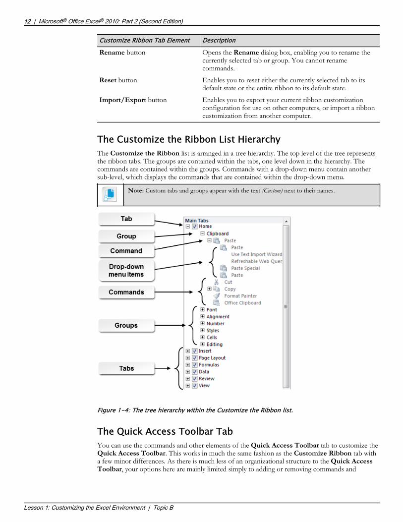
The Customize the Ribbon List HierarchyThe Customize the Ribbon list is arranged in a tree hierarchy. The top level of the tree representsthe ribbon tabs. The groups are contained within the tabs, one level down in the hierarchy. Thecommands are contained within the groups. Commands with a drop-down menu contain anothersub-level, which displays the commands that are contained within the drop-down menu.

Note: Custom tabs and groups appear with the text (Custom) next to their names.

Figure 1-4: The tree hierarchy within the Customize the Ribbon list.

The Quick Access Toolbar TabYou can use the commands and other elements of the Quick Access Toolbar tab to customize theQuick Access Toolbar. This works in much the same fashion as the Customize Ribbon tab witha few minor differences. As there is much less of an organizational structure to the Quick AccessToolbar, your options here are mainly limited simply to adding or removing commands and



The Customize theRibbon List Hierarchy

The Quick AccessToolbar Tab

Do Not D

uplicate

or Dist

ribute

rearranging the order of commands. But you can add sections to the Quick Access Toolbar for thepurpose of organizing commands by using visual borders called separators.

Figure 1-5: The Quick Access Toolbar tab.

The following table describes the various elements of the Quick Access Toolbar tab.

Quick Access Toolbar Tab Element Description

Choose commands from drop-down menu

Selects which commands are displayed in the Choosecommands from list.

Choose commands from list Displays the commands you can add to the Quick AccessToolbar.

Customize Quick Access Toolbardrop-down menu

Selects whether Quick Access Toolbar customizationsapply to all workbooks or just the current workbook.

Customize Quick Access Toolbarlist

Displays the current Quick Access Toolbar configuration.

Add button Adds commands selected in the Choose commands fromlist to the Quick Access Toolbar.

Remove button Removes the currently selected command from the QuickAccess Toolbar.

Move Up button Moves the currently selected command up one place in theCustomize Quick Access Toolbar list.

Move Down button Moves the currently selected command down one place inthe Customize Quick Access Toolbar list.

Reset button Enables you to reset either the Quick Access Toolbar orthe Quick Access Toolbar and the ribbon to the defaultconfiguration.



Do Not D

uplicate

or Dist

ribute

Quick Access Toolbar Tab Element DescriptionImport/Export button Enables you to export your current Quick Access Toolbar

customization configuration for use on other computers orimport a Quick Access Toolbar customization fromanother computer.

The Customize Quick Access Toolbar MenuYou can also add or remove commands from the Quick Access Toolbar, or QAT, by using theCustomize Quick Access Toolbar menu, but your options here are a bit more limited. From theCustomize Quick Access Toolbar menu, you can add or remove commands from a limited set ofsome of the most commonly used Excel commands. You cannot rearrange commands or addseparators to the QAT from here.The Customize Quick Access Toolbar menu also provides you with the ability to move the QATso it is positioned below the ribbon. To access the Customize Quick Access Toolbar menu, select

the Customize Quick Access Toolbar button to the right of the QAT.

Figure 1-6: Check or uncheck the command options in the Customize Quick Access Toolbarmenu to add them to or remove them from the QAT.

Access the Checklist tile on your LogicalCHOICE course screen for referenceinformation and job aids on How to Customize the Ribbon and the Quick AccessToolbar.



The Customize QuickAccess Toolbar Menu

Do Not D

uplicate

or Dist

ribute

ACTIVITY 1-2Customizing the Ribbon and the Quick AccessToolbar

Before You BeginExcel 2010 is open.

ScenarioThere are a few other modifications you would like to make to the Excel environment to help youwork more efficiently. Because you create and reopen a number of workbook files daily, you wouldlike to have access to the New and Open commands on the Quick Access Toolbar. And, as youmost frequently use the commands on the Home tab and the Formulas tab, you want to placethem next to each other on the ribbon. Finally, there is a command you know you will be using a lotin the future, so you decide to add it to both the ribbon and the Quick Access Toolbar.

1. Add the New and Open commands to the Quick Access Toolbar.

a) On the right side of the Quick Access Toolbar, select the Customize Quick Access Toolbar button.

b) From the Customize Quick Access Toolbar menu, verify the New command is selected.c) Add the Open command to the Quick Access Toolbar.

2. Move the Formulas tab so that it is to the right of the Home tab on the ribbon.a) Select File→Options.b) In the Excel Options dialog box, select the Customize Ribbon tab.c) In the Customize the Ribbon drop-down menu, ensure that Main Tabs is selected.d) In the Customize the Ribbon list, select Formulas.



Remind students theycan use the Opencommand on the QuickAccess Toolbar for therest of the course toopen the data files.

Do Not D

uplicate

or Dist

ribute

e) Select the Move Up button twice, so that the Formulas tab appears just below the displayed groupsof the Home tab.

f) Select OK and then verify that the Home tab and the Formulas tab appear next to each other on the

ribbon.

3. Add the Insert PivotTable command to the Quick Access Toolbar.a) Select File→Options.b) In the Excel Options dialog box, select the Quick Access Toolbar tab.c) From the Choose commands from drop-down menu, select All Commands.d) In the Choose commands from list, scroll down and select Insert PivotTable.e) Select Add.

Note: It is okay to leave the Excel Options dialog box open here.

4. Add the PivotTable and Insert Slicer commands to the ribbon in a custom group.a) In the Excel Options dialog box, select the Customize Ribbon tab.b) In the Customize the Ribbon drop-down menu, ensure that Main Tabs is selected.c) In the Customize the Ribbon list, in the Home tab hierarchy, select Editing and then, below this list,

select New Group.

d) Select Rename.e) In the Rename dialog box, in the Display name field, type PivotTable and then select OK.f) In the Choose commands from drop-down menu, ensure that Popular Commands is selected.g) In the Choose commands from list, scroll down, select PivotTable, and then select Add.



Remind the studentsthat the New Groupcommand inserts a newgroup after the currentselection.

If students ask about thediscrepancy, let themknow that the commandsimply has a differentname for the QAT andthe ribbon. It is still thesame commandfunctionally.If students ask, remindthem that all customtabs and groups willhave the text (Custom)next to their names.

Do Not D

uplicate

or Dist

ribute

h) Ensure that the PivotTable command now appears in the newly created PivotTable (Custom) group.

i) In the Choose commands from drop-down menu, select All Commands.j) In the Choose commands from list, scroll down, select Insert Slicer, and then select Add.k) In the Excel Options dialog box, select OK.

5. Verify that the Insert PivotTable command now appears on the Quick Access Toolbar and thePivotTable and Insert Slicer commands now appear in the PivotTable group on the Home tab.



Do Not D

uplicate

or Dist

ribute

TOPIC CEnable Excel Add-InsExcel 2010 is loaded with a robust set of tools and features meant to help you get the most out ofyour data. If the default functionality suits all of your needs, you may not need to customize Excelbeyond the option or UI changes you have already made. But there are entire sets of additionalfunctionality available to Excel users who need a little more power in their Excel installations. Ifyou're one of these users, you'll need to know how to access the available additional functionality.Fortunately, Excel 2010 makes it easy to activate only the additional tools and features you need toperform your job. Taking a few moments now to understand how to find and activate theseadditional tools and features means you'll be able to call upon Excel's additional capabilitieswhenever the need arises.

Add-InsAdd-ins are supplemental programs for Microsoft Office applications that provide additional featuresand functionality not available in a standard installation. Some add-ins, such as the Analysis ToolPakand the Solver add-in, come installed with Excel but are simply not activated by default. Other add-ins can be downloaded from Microsoft Office Online and then activated. You can also developcustom add-ins to enhance Excel's functionality, if you have the programming acumen to do so.Add-ins must be enabled for you to have access to their features and functionality.

The Add-Ins TabYou can view and manage your Excel add-ins from the Add-Ins tab on the Excel Options dialogbox. From here you can view all add-ins that are installed on your computer, and all add-ins that areboth installed and enabled. This is also where you can access dialog boxes for the various add-intypes, which allow you to enable and disable add-ins as needed.


Lesson 1: Customizing the Excel Environment | Topic C

The Add-Ins Tab

Do Not D

uplicate

or Dist

ribute

Figure 1-7: The Add-Ins tab.

The following table describes some of the key elements of the Add-Ins tab.

Add-Ins Tab Element Allows You To

Active Application Add-inssection

View a list of all add-ins currently installed and enabled onyour computer.

Inactive Application Add-inssection

View a list of all add-ins that are currently installed on yourcomputer but that are disabled.

Type column View add-in types. These typically give you a clue to thegeneral functionality or features the add-in provides forExcel.

Add-in information View additional information about the currently selected add-in.

Manage drop-down menu Access the dialog boxes for the various add-in types. Fromthese dialog boxes, you can enable or disable add-ins asneeded.

Note: For more information on adding further capabilities to Excel, watch the LearnTOExpand Excel's Capabilities Using Add-Ins presentation from the LearnTO tile on theLogicalCHOICE Course screen.

Access the Checklist tile on your LogicalCHOICE course screen for referenceinformation and job aids on How to Enable Add-Ins.



You may want to showLearnTO Expand Excel'sCapabilities Using Add-Ins from theLogicalCHOICE Coursescreen or have studentsnavigate out to theCourse screen andwatch it themselves as asupplement to yourinstruction. If not, pleaseremind students to visitthe LearnTOs for thiscourse on theirLogicalCHOICE Coursescreen after class forsupplementalinformation andadditional resources.

Do Not D

uplicate

or Dist

ribute

ACTIVITY 1-3Enabling Excel Add-Ins


ScenarioThere is one final Excel customization you wish to make. As you frequently work with currencyfigures for European offices and authors, you would like to add the ability to work with currencyfigures in terms of the Euro. You decide to activate the Euro Currency Tools add-in.

1. Select File→Options.

2. In the Excel Options dialog box, select the Add-Ins tab.

3. At the bottom of the Add-ins section, in the Manage drop-down menu, ensure that Excel Add-ins isselected and then select Go.

4. In the Add-Ins dialog box, check the Euro Currency Tools check box and then select OK.

5. Ensure that the Euro Currency Tools add-in is now enabled.a) Open the Excel Options dialog box and select the Add-Ins tab.b) In the Add-ins section, ensure that the Euro Currency Tools add-in appears in the Active Application

Add-ins list.

6. Close the Excel Options dialog box.



Do Not D

uplicate

or Dist

ribute

SummaryIn this lesson, you customized the Excel environment by configuring options and settings,customizing the ribbon and the QAT, and by managing add-ins. As you develop your Excel skillsand experience, you will almost certainly find that you like some of Excel's default functionality,while, at other times, it will seem to hold you back. With the ability to tailor the Excel environmentto suit your needs and your personal work flow, you'll have Excel working harder for you, which willmake you more efficient and productive.

What changes do you anticipate making to the Excel environment to help you work more efficiently?

A: Answers will vary, but most students will likely add a few commands their specific role requires them touse frequently to the QAT or an often-accessed ribbon tab. People who work in highly specializedfields may be likely to activate some of Excel's add-ins.

Do you think you'll most likely add customizations to the QAT or the ribbon? Why?

A: Answers will vary, largely depending on how students use Excel. People who create numerousworkbooks, frequently, and for fairly common tasks may be more likely to simply add a few file-relatedcommands to the QAT. Users who perform numerous, complex tasks in a few large workbooks aremore likely to create highly customized ribbons.

Note: Check your LogicalCHOICE Course screen for opportunities to interact with yourclassmates, peers, and the larger LogicalCHOICE online community about the topics covered inthis course or other topics you are interested in. From the Course screen you can also accessavailable resources for a more continuous learning experience.


Lesson 1: Customizing the Excel Environment |

Encourage students touse the socialnetworking toolsprovided on theLogicalCHOICE Homescreen to follow up withtheir peers after thecourse is completed forfurther discussion andresources to supportcontinued learning.

Do Not D

uplicate

or Dist

ribute

Do Not D

uplicate

or Dist

ribute

Creating AdvancedFormulasLesson Time: 1 hour, 45 minutes

Lesson ObjectivesIn this lesson, you will create advanced formulas. You will:

• Use range names in formulas.

• Use specialized functions.

• Use array formulas.

Lesson IntroductionYou already know how to get Excel to perform simple calculations to make your job easier.However, manually entering formulas will take you only so far. The commonly usedfunctions in Excel may not be enough to handle more complex data analysis needs. As youprogress with Excel, and as you are called upon to provide a deeper understanding of yourorganizational data to organizational decision makers, you'll need to know how to ask Excelmore complex questions about your data and to get the answers you expect.Of course, the more complex your data analysis tasks are, the more complexity you're likelyto need in your formulas and functions. This means that you'll need to know how to talk toExcel at a higher level to get the most out of your data. As with mathematics in general, andall forms of computer programming, understating the language Excel speaks is the key tohaving conversations with Excel and getting the answers you need.

2

Do Not D

uplicate

or Dist

ribute

TOPIC AUse Range Names in FormulasIt is a rare individual who works in a bubble with little to no contact with other people. As such, it ishighly likely that you will not be the only person working with and analyzing data with yourworkbooks. This means it's essential that everyone working in the same workbook understandsprecisely what the formulas and functions are calculating. Although cell and range references makeincluding figures in calculations and reusing those figures in multiple calculations easy, it's not alwaysapparent at first glance what the formula is calculating. Manually typing or selecting cell and rangereferences in large workbooks with many formulas can become tedious and potentially lead toerrors. Wouldn't it be nice if there were a clearer, simpler way to include cell and range references inExcel?Excel 2010 allows you to name ranges for use in functions and formulas. Mastering this key trick tocreating formulas and functions is an easy way to use the same ranges over and over in yourworksheets and to make those formulas and functions clearer to others who view and work in yourworkbook files. This is truly one of the most powerful features of Excel. Once you know how toname ranges and refer to those ranges by name in your formulas, you'll be developing complex,interconnected worksheets in no time.

Cell and Range NamesCell names and range names are exactly what they sound like. They are meaningful names you assign toa given cell or range to make it easier to both understand what calculations are being performed in aformula and reuse the references for a number of purposes. Take a look at the following image,which shows two versions of the same formula, one using cell references and one using named cells.

Figure 2-1: The same formula using cell references and names.

Now, imagine that you open this workbook months, or even years, after you created it. At firstglance, which formula is easier to interpret? And, if you share this workbook with a colleague, whichwould make it clearer to the workbook recipient what her or she is looking at? It's pretty clear howpowerful a feature this is.

Note: Cell and range references aren't the only items you can name in Excel. You can nameother objects, such as tables and even formulas themselves. Collectively, the names you assign toall of these items are known as defined names.

In short, cell and range names are concise, descriptive names you can assign to cells or ranges forthe purpose of making formulas easier to read and maintain. You can assign a name to both


Lesson 2: Creating Advanced Formulas | Topic A

Cell and Range Names

Do Not D

uplicate

or Dist

ribute

contiguous ranges and noncontiguous ranges. Names refer to absolute references by default but youcan change those to relative references to facilitate the reuse of formulas.

Note: It may be a good idea to indicate in a name whether the reference is absolute or relative,as the name will be displayed precisely as you created it regardless of which type of reference itcontains.

Although you can come up with an incredible array of different names, there are some rules youmust follow:• Names must begin with a letter, an underscore, or a backslash.• After the first character, names can contain letters, numbers, periods, and underscores.• Names cannot contain spaces.• Names cannot be the same as a cell or a range reference. For example, you cannot use $A$1 as a

name.• Names have a defined scope, either to a worksheet or a workbook, and must be unique within

that scope.• Names can contain up to 255 total characters.• Excel does not recognize casing differences for names. So, within the same scope, you cannot,

for example, create both SalesTotals and salestotals as names.• You can use a single letter as a name, you cannot do so by using either C or R, either uppercase

or lowercase, as these are used as shorthand for selecting an entire row or an entire column inother Excel features.

Names and the Name BoxThere are several methods you can use to create names in Excel 2010. The most direct of these is touse the Name Box. To name a cell or a range, you can simply select the desired cell or range andthen type the desired name in the Name Box. Once you've created named cells and ranges, you canaccess those cells and ranges from the Name Box drop-down menu. This is a quick way to select acell or range that you've already named. Additionally, if you manually select a named cell or range ona worksheet, the name, not the cell reference, is displayed in the Name Box. Names created in theName Box, by default, have "Workbook" as their scope.

Figure 2-2: Named ranges in the Name Box.

The New Name Dialog BoxYou can also name cells or ranges by using the New Name dialog box. The advantage here is thatyou have greater control over configuring precisely what the name refers to. You can access theNew Name dialog box by selecting Formulas→Defined Names→Define Name.



Names and the NameBox

The New Name DialogBox

Do Not D

uplicate

or Dist

ribute

Figure 2-3: The New Name dialog box gives you greater control over naming cells and ranges.

The following table describes the various elements of the New Name dialog box.

New Name Dialog Box Element Allows You To

Name field Enter a name for the cell or range.

Scope drop-down menu Assign a scope to the name. This can be either the entireworkbook or a particular worksheet. You cannot create twoidentical names within the same scope. You can, however, createidentical names for both a worksheet and the workbookcontaining that worksheet. On the worksheet, the name that hasthe worksheet as its scope will take precedence. On all otherworksheets, the name that has the workbook as its scope willtake precedence.

Comment field Enter a brief description of the named cell or range to helpclarify its purpose.

Refers to field View or edit the name's reference. Whatever cell or range isselected when you open the New Name dialog box will bedisplayed as an absolute reference in the Refers to field bydefault.

The Create from Selection CommandAnother method you can use to name ranges is the Create from Selection command. Thiscommand enables you to quickly and easily create a single range name or multiple range names atonce, based on the range you currently have selected. The Create from Selection command doesnot work for naming individual cells. By default, named ranges you create by using this commandhave "Workbook" as their scope.When you select a range and then select the Create from Selection command, Excel opens theCreate Names from Selection dialog box, which allows you to select the cells from which Excelwill create the names. This feature works best for ranges with clearly defined content types andappropriately labeled row and column headers. You may get unexpected results or error messages ifheaders don't align with Excel's naming conventions. If you use the Create from Selectioncommand when a range in a single row or column in selected, Excel will create a single namedrange. If a range that covers multiple rows and columns is selected, Excel will create a series ofnamed ranges based on the cell selection and the option you check in the Create Names fromSelection dialog box. The cells from which Excel creates the names are not included in the rangereference for the named ranges. The Create from Selection command is available in the Defined



The Create fromSelection Command

Do Not D

uplicate

or Dist

ribute

Names group on the Formulas tab. You can also use the Ctrl+Shift+F3 keyboard shortcut toopen the Create Names from Selection dialog box.

Figure 2-4: Use the Create from Selection command to quickly create multiple named ranges.

The Name Manager Dialog BoxAs most workbooks are dynamic, changing documents, it stands to reason that you will likely haveto edit named cells and ranges from time to time. For example, if you need to add rows to a range ofdata, you will likely want named column ranges within that range of data to include the new rows.Excel 2010 provides the Name Manager dialog box, a tool you can use to view and manage all ofthe named objects in your workbooks. From here, you can rename, edit, and delete existing namedobjects, and access the New Name dialog box to create new named cells or ranges. You cannot,however, change the scope of an existing cell or range name by using the Name Manager dialogbox. To do this, you can delete the existing name and create a new one with the desired scope. TheName Manager dialog box also displays a Filter command, which you can use to filter the displayof existing names. Use the Filter command, for example, to view only those names that have theentire workbook as their scope, names that have a particular worksheet as their scope, or namescontaining errors. You can access the Name Manager dialog box by selectingFormulas→Defined Names→Name Manager.



The Name ManagerDialog Box

Do Not D

uplicate

or Dist

ribute

Figure 2-5: The Name Manager dialog box.

Access the Checklist tile on your LogicalCHOICE course screen for referenceinformation and job aids on How to Name and Edit Ranges.



Do Not D

uplicate

or Dist

ribute

ACTIVITY 2-1Naming and Editing Ranges

Data FileC:\091019Data\Creating Advanced Formulas\author_data.xlsx


ScenarioYour supervisor has asked you to provide her with information about total income by author. Youhave raw data for Fuller's authors tracked in a worksheet that contains information about how longeach author has been with the company, how many titles each currently has published throughFuller and Ackerman, how many total books each author has sold, and the price at which eachauthor's books sell. Before you perform the calculations to determine how much each author hascontributed to Fuller's income, you decide to name the various ranges for use in formulas to makethe worksheet easier for your supervisor, and anyone else who may end up using it, to interpret.

1. Open the author_data.xlsx workbook.

2. Use the Name Box to create a named range in the AuthorID column.

a) Select cell A2 and press Ctrl+Shift+down arrow.b) Select the Name Box, type Author_ID and press Enter.

3. Use the New Name dialog box to create a named range in the Initial Contract Date column.a) Select cell B2 and press Ctrl+Shift+down arrow.b) Select Formulas→Defined Names→Define Name.c) In the New Name dialog box, in the Name field, type Initial_Contract_Dated) Ensure that Workbook is selected in the Scope drop-down menu.e) Ensure that the Refers to field displays the following range reference: =Authors!$B$2:$B$94.f) Select OK.

4. Use the Create from Selection command to create a named range in the Years Under Contract column.

a) Select the range C1:C94 and then select Formulas→Defined Names→Create from Selection.b) In the Create Names from Selection dialog box, ensure that the Top row check box is checked and

then select OK.

5. Verify that the three named ranges exist by selecting the Name Box down arrow and confirming that thenames appear as expected.

6. Use the Create from Selection command to create named ranges for the final three columnssimultaneously.a) Select cell D1 and press Ctrl+Shift+right arrow.b) Press Ctrl+Shift+down arrow.c) Select Formulas→Defined Names→Create from Selection.d) In the Create Names from Selection dialog box, ensure that the Top row check box is checked and

then select OK.e) Verify that Excel created three unique named ranges for the final three columns.



Let the students knowthat Ctrl+Shift+downarrow is the keyboardshortcut for selecting allcontiguously populatedcells below the selectedcell or range.

This is a goodopportunity to quiz theclass to see if they knowwhat the significance ofthe text "Authors!" isbefore the rangereference. The answer:It is the worksheetreference for the range.In step 4a, ensure thatstudents select therange C1:C94, and notC2:C94.Do N

ot Duplic

ate or D

istrib

ute

7. Edit the range names for the Number of Titles in Print and Number of Books Sold columns to makethem a bit shorter.a) Select Formulas→Defined Names→Name Manager.b) In the Name Manager dialog box, select the Number_of_Books_Sold range name and then select

Edit.c) In the Edit Name dialog box, in the Name field, type No_of_Books_Sold and select OK.d) Change the range name Number_of_Titles_in_Print to No_of_Titles_in_Printe) Close the Name Manager dialog box.f) Verify that the names have changed as expected.

8. Save the workbook to the C:\091019Data\Creating Advanced Formulas folder as my_author_data.xlsx

Cell and Range Names in FormulasAlthough it's certainly helpful to be able to name a range or a cell for easy navigation, the real powerof this feature lies in the ability to easily identify references in formulas and to quickly and accuratelyinsert references into multiple formulas. Once you've defined a name, you can simply use the namein place of a standard cell or range reference in any formula or function.

Figure 2-6: Named cells and ranges make it easier to identify the purpose of formulas and toenter cell and range references more accurately.

As with many of the features and functions in Office applications, Excel provides several ways toperform a task. Such a task, in Excel, is inserting cell and range names in formulas and functions.The most common of these many methods are manually typing the name in a formula or function,using the Use in Formula command, and using the Formula AutoComplete feature. Let's look ateach of these in some detail.

Manually Entering Cell or Range NamesThe most direct method for including cell or range names instead of references in formulas orfunctions is to simply type them. Wherever you would normally enter a cell or range reference, youcan type a defined name instead. The formula will reference the cell or range by name just as itwould if you typed the cell or range reference, and your calculation results will be the same.

Note: It is important to note that you can still type the cell or range references for a named cellor range in a formula, and they will still appear as cell or range references.

You can also manually select a cell or range that you've applied a name to directly on a worksheet toenter it into a formula just as you would with any unnamed range or cell. When you do this, Excelautomatically displays the name, not the reference, though.

The Use in Formula Command MethodExcel 2010 includes a ribbon command you can use to insert cell and range names into formulasand functions: the Use in Formula command. As with manually typing a cell or a range name, youcan use this method anywhere you would normally enter a range or cell reference in a formula.Instead of typing the name, you simply select the Use in Formula command, and then select thedesired defined name from the drop-down menu. You can access the Use in Formula command byselecting Formulas→Defined Names→Use in Formula.



Cell and Range Namesin Formulas

The Use in FormulaCommand MethodDo N

ot Duplic

ate or D

istrib

ute

Figure 2-7: The Use in Formula command displays all valid defined names for use in formulasand functions.

From the Use in Formula drop-down menu, you can also select Paste Names, which opens thePaste Name dialog box. This provides you with yet another option for selecting a named cell orrange. The added benefit here is that there is a keyboard shortcut, F3, that you can use to quicklyopen the Paste Name dialog box.

The Formula AutoComplete MethodYou already know the Formula AutoComplete feature can help you enter functions into worksheetcells without having to type the full function name. Well, the Formula AutoComplete feature canalso help you enter range and cell names into formulas and functions, and it works in the exact sameway. As you type a formula or a function into a cell, whether directly into the cell or by using theFormula Bar, and you begin to type a cell or range name, the Formula AutoComplete featureautomatically opens the same pop-up menu that appears when you type a function name. You canselect any valid named cells or ranges from the pop-up menu to enter into the formula or function.The pop-up menu automatically filters the available defined names just as it would Excel functions.You can differentiate between functions and defined names in the Formula AutoComplete feature

by viewing the icon next to each option. Functions will display the Insert Function icon ,

whereas defined names will display an icon that looks like a paper tag . Once you've entered thecell or range name, you simply continue entering the rest of the formula or function as you normallywould.

Figure 2-8: Adding a range name by using the Formula AutoComplete feature.

Access the Checklist tile on your LogicalCHOICE course screen for referenceinformation and job aids on How to Use Defined Names in Formulas and Functions.



The FormulaAutoComplete Method

Do Not D

uplicate

or Dist

ribute

ACTIVITY 2-2Using Defined Names in a Formula

Before You BeginThe my_author_data.xlsx workbook is open.

ScenarioNow that you have created named ranges for the various columns, you will use them to enterfunctions to provide your supervisor with the income-per-author data she has asked for. For thepurposes of this worksheet, Fuller and Ackerman defines income earned as the number of bookssold multiplied by the sell price. To maintain consistency and to facilitate using the income earneddata in future calculations, you decide to name the range for the calculation results as well.

1. Add a column label for the income earned data.a) Select cell G1.b) Type Income Earned and press Enter.

2. Use range names to enter a formula that will calculate the income earned.a) Ensure that cell G2 is selected.b) Type =noc) From the Formula AutoComplete pop-up menu, double-click No_of_Books_Sold.

d) Type an asterisk ( * ) and select Formulas→Defined Names→Use in Formula→Sell_Price.

e) Press Ctrl+Enter.



Remind students thatpressing Ctrl+Enterenters the formula andkeeps the same cellactive. This will helpthem view the results ofentering the formula.

Do Not D

uplicate

or Dist

ribute

f) Verify that the formula behaves as expected, and that it displays defined names instead of cellreferences.

3. With cell G2 selected, select the Home tab and, from the Number Format drop-down menu in theNumber group, select Currency.

4. Adjust the width of column G to accommodate the new formatting.

5. Copy the formula for all authors on the worksheet.a) Ensure that cell G2 is still selected.b) Double-click the fill handle in the bottom-right corner of the cell.

c) Press Ctrl+. (the period key) to invert the active cell in the range and verify that Excel copied the

formula in the entire range G2:G94.d) Press Ctrl+. again to return the active cell back to the top of column G.e) If necessary, re-adjust the width of column G to accommodate all of the entries.

6. Assign the name Income_Earned to the range G2:G94.

7. Save the file.



Do Not D

uplicate

or Dist

ribute

TOPIC BUse Specialized FunctionsYou are already familiar with the most basic functions and formulas in Excel. You're also likelyaware that there are far more complex tasks you can perform in Excel beyond adding up rows andcolumns and multiplying the sum by some other figure. As you progress in your knowledge ofExcel, and in your career, you are likely to be called upon to perform more and more complexnumber crunching and data analysis tasks. As such, you'll need to have a much better handle onExcel functions than you did previously.Excel contains an incredibly vast array of built-in functions that you can use to perform a staggeringnumber of calculations. You'll need to know how to locate specific functions when performingspecific tasks. You'll need to know a great deal about the syntax of these functions if you expectExcel to provide answers to your questions. Taking the time now to build a foundationalunderstanding of how some of the more specialized and complex functions work, will give you thetools you need to ask Excel more and more complex questions related to your data.

Function CategoriesYou will find every built-in Excel function in the Function Library group on the Formulas tab.Here, the vast collection of available functions is organized into task-related categories. There are 11standard categories of included functions and this can be expanded by installing certain Excel add-ins.

Note: You have to access several of these categories from the More Functions drop-downmenu in the Function Library group.

Figure 2-9: The Function Library group on the Formulas tab.

Function Library Category Contains Functions For

Financial Calculating financial figures such as accrued interest, rates of return,monthly payments, and asset depreciation.

Logical Returning a value of either TRUE or FALSE for a given set ofcriteria. Use these in conjunction with other functions or formulasto perform calculations based on certain conditions. Basically, thisadds a decision-making dimension to Excel functions and formulas.

Text Manipulating text. For example, you can use these functions toconvert text to all uppercase or all lowercase, or to join text stringsfrom multiple cells.

Date & Time Working with dates and times. For example, you can use thesefunctions to simply return the current date, or to calculate thenumber of working days in a given period.

Lookup & Reference Finding specific values in a table or a given range.


Lesson 2: Creating Advanced Formulas | Topic B

Function Categories

Do Not D

uplicate

or Dist

ribute

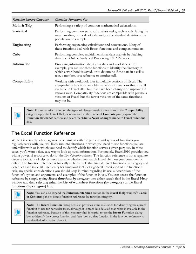
Function Library Category Contains Functions ForMath & Trig Performing a variety of common mathematical calculations.

Statistical Performing common statistical analysis tasks, such as calculating themean, median, or mode of a dataset, or the standard deviation of apopulation or a sample.

Engineering Performing engineering calculations and conversions. Many ofthese functions deal with Bessel functions and complex numbers.

Cube Performing complex, multidimensional data analysis by fetchingdata from Online Analytical Processing (OLAP) cubes.

Information Providing information about your data and worksheets. Forexample, you can use these functions to identify the directory inwhich a workbook is saved, or to determine if the data in a cell istext, a number, or a reference to another cell.

Compatibility Working with workbook files in multiple versions of Excel. Thecompatibility functions are older versions of functions that are stillavailable in Excel 2010 but that have been changed or improved invarious ways. Compatibility functions are compatible with previousversions of Excel, but the newer versions of the same functionsmay not be.

Note: For more information on the types of changes made to functions in the Compatibilitycategory, open the Excel Help window and, in the Table of Contents pane, expand theFunction Reference section and select the What's New: Changes made to Excel functionslink.

The Excel Function ReferenceWhile it is certainly advantageous to be familiar with the purpose and syntax of functions youregularly work with, you will likely run into situations in which you need to use functions you areunfamiliar with or in which you need to identify which function serves a given purpose. In thesecases, you'll want a fast, easy way to look up such information. Fortunately, Excel 2010 provides youwith a powerful resource to do so: the Excel function reference. The function reference is not a separate,discrete tool; it is a Help resource available whether you search Excel Help on your computer oronline. The function reference is basically a Help article that lists all Excel functions by category anddescribes each in detail. Each entry for functions includes a general description of the function'stask, any special considerations you should keep in mind regarding its use, a description of thefunction's syntax and arguments, and examples of the function in use. You can access the functionreference by simply typing Excel functions by category into either search field in the Excel Helpwindow and then selecting either the List of worksheet functions (by category) or the Excelfunctions (by category) link.

Note: You can also expand the Function reference section in the Excel Help window's Tableof Contents pane to access function references by function category.

Note: The Insert Function dialog box also provides some assistance for identifying the correctfunction to use for particular tasks, although it is much less detailed than what is available in thefunction reference. Because of this, you may find it helpful to use the Insert Function dialogbox to identify the correct function and then look up that function in the function reference tosee detailed information about it.



The Excel FunctionReference

Do Not D

uplicate

or Dist

ribute

Figure 2-10: Use the function reference to examine any function in detail.

Access the Checklist tile on your LogicalCHOICE course screen for referenceinformation and job aids on How to Locate Functions by Using the Excel FunctionReference.

Logical Operator BasicsBefore you examine the syntax of more Excel functions, there is a group of operators you may notyet be familiar with in terms of Excel: logical operators. You might, however, remember these as themathematical symbols that indicate conditions such as one figure being greater than or less thananother. As you advance in your understanding of Excel functions, you will find that these logicaloperators form the basis for using many of Excel's functions and taking advantage of many of itsfeatures. For now, it will be enough to simply understand what these logical operators mean. Thefollowing table describes what each of the operators means in Excel functions.

Logical Operator Meaning

= Equal to

< Less than

> Greater than

<= Less than or equal to

>= Greater than or equal to

<> Not equal to



Inform the students thatyou will be coveringlogical operators inmuch greater detail inthe topic on using textand logical functions.This introduction is justenough for the studentsto be able to understandusing functions such asSUMIF andAVERAGEIF.

Do Not D

uplicate

or Dist

ribute

Function SyntaxBy now, you have likely familiarized yourself with the syntax for a number of basic Excel functionsand have had some opportunity to use them regularly. You'll remember that a function's syntaxdefines the structure of the function and identifies the required and optional arguments you can useto complete it. As you advance in your Excel proficiency, you'll want to add to your lexicon offamiliar functions so you don't have to look up functions frequently as you develop yourworkbooks. Here is an overview of some of the commonly used Excel functions you may notalready be familiar with.

The SUMIF FunctionSyntax: =SUMIF(range, criteria, [sum_range])

Note: Remember that, in Excel function syntax, arguments within square brackets ( [ ] ) areoptional.

Description: This function adds the values in a given range that meet some specific criteria. Use thisfunction, for example, if you'd like to add all sales figures greater than a particular value in a column.In the function's syntax, range is the range of cells to which the criteria is applied, criteria is thecondition that must be met, and sum_range is the range of cells from which to add values if youwant that range to differ from the one specified in the range argument. If you do not specify arange for the optional sum_range argument, the function sums the qualifying values from the cellsspecified in the range argument.

Note: The criteria argument must be enclosed in quotation marks (" ") if it contains text,mathematical operators, or logical operators. This is common among the various functions thatcontain the criteria argument.

Examples of values that can be added to the SUMIF function are included in the following table.

To Add These Values Enter This Function

All numbers greater than 10 in the range A1:A10. =SUMIF(A1:A10, ">10")

All numbers in the range B1:B10 that correspond to the textentry "Bill" in the range A1:A10. In other words, if you have alist of names in column A, and corresponding sales values incolumn B, this function would add all figures for peoplenamed Bill.

=SUMIF(A1:A10, "Bill", B1:B10)

Every instance of the value 5 in the range A1:A10. =SUMIF(A1:A10, 5)

The AVERAGEIF FunctionSyntax: =AVERAGEIF(range, criteria, [average_range])Description: This function returns the arithmetic mean of every cell in a range that meets thespecified criteria. You would use this formula, for example, if you wanted to find the average valueof all sales figures that are less than or equal to some specified amount. In the function's syntax,range is the range of cells to which the criteria is applied, criteria is the condition that must be met,and average_range is the range of cells from which the mean is calculated if you want that range todiffer from the one specified in the range argument. If you do not specify a range in the optionalaverage_range argument, the function finds the average of the qualifying values from the cellsspecified in the range argument.Examples of values that can be added to the AVERAGEIF function are included in the followingtable.



This is a goodopportunity to facilitate adiscussion on the valueof some of the morespecialized Excelfunctions. Of keyimportance here is thedifference betweenusing Excel as a simplecalculator and using it asa data analysis tool.Due to time constraints,you may not wish tocover all of thesefunctions in detail inclass. Considerinforming students thatthey can use this contentfor future reference.

Do Not D

uplicate

or Dist

ribute

To Find the Average of These Values Enter This Function

All numbers less than or equal to 20 in the rangeA1:A10.

=AVERAGEIF(A1:A10, "<=20")

All numbers in the range C1:C10 that correspondto a value that is greater than or equal to 100,000 inthe range B1:B10. For example, if the range A1:A10contains authors' names, the range B1:B10 displaystotal sales per author, and the range C1:C10contains the authors' sales commissions, then thisfunction would return the average salescommission for authors who sold $100,000 ormore worth of books.

=AVERAGEIF(B1:B10, ">=100000",C1:C10)

Note: When including numeric values in function arguments, do not use commas to separatethe numerals at each magnitude of 1,000. Excel will read this as the end of one argument and thebeginning of the next argument.

The COUNTIF FunctionSyntax: =COUNTIF(range, criteria)Description: This function counts the number of cells in the specified range that contain datamatching the specified criteria. You could use this function, for example, to count the number ofsales reps who have met or exceeded a particular sales target or the number of people in yourorganization named "Betty." In the function's syntax, range is the range of cells to which the criteriais applied and from which the qualifying entries are counted, and criteria is the condition that mustbe met for an entry to be counted. The COUNTIF function counts values from within the rangeargument only.Examples of values that can be added to the COUNTIF function are included in the followingtable.

To Count the Number of Cells Containing Enter This Function

Values greater than or equal to 1,000 in the rangeA1:A10.

=COUNTIF(A1:A10, ">=1000")

An instance of the value 13 in the range B1:C20. =COUNTIF(B1:C20, 13)

The name "Fred" in the range A1:A350 =COUNTIF(A1:A350, "Fred")

IFS FunctionsThe AVERAGEIF, COUNTIF, and SUMIF functions all have an equivalent function that enablesyou to perform the respective calculations on a dataset that meets more than one specified criterion.These are the AVERAGEIFS, COUNTIFS, and SUMIFS functions, respectively. The maindifferences in the function syntaxes for the "IFS" functions are that the arguments are in a differentorder and that there are additional, optional arguments for the additional criteria. Otherwise, theyfunction essentially the same as their counterparts. Here is the function syntax for each of these"IFS" functions:=AVERAGEIFS(average_range, criteria_range1, criteria1, [criteria_range2], [criteria2], ...)=COUNTIFS(criteria_range1, criteria1, [criteria_range2], [criteria2], ...)=SUMIFS(sum_range, criteria_range1, criteria1, [criteria_range2], [criteria2], ...)

COUNTASyntax: =COUNTA(value1, [value2], ...)



Do Not D

uplicate

or Dist

ribute

Description: This function counts the number of cells specified by the arguments that are notempty. This function does not distinguish between the various content types, such as formulas,values, and text. The arguments can be either cell or range references or both.Examples of values that can be added to the COUNTA function are included in the following table.

To Count the Number of Non-Empty Cells Enter This Function

In the range A1:A50 =COUNTA(A1:A50)

In the range A1:B30 =COUNTA(A1:B30)

In the range A1:A10 and in cells B3 and C9 =COUNTA(A1:A10, B3, C9)

The PMT functionSyntax: =PMT(rate, nper, pv, [fv], [type])Description: This function calculates the payments for a loan with a fixed interest rate and fixedpayment periods. You can use this function, for example, to calculate your payments for a fixed-ratemortgage, auto loan, or student loan. In the function's syntax, here are the required arguments: rateis the loan's fixed interest rate, nper is the total number of payments for the loan (for example,monthly payments for a three-year loan occur 36 times), pv is the present value (principal) of theloan. There are two optional arguments for the function: fv (future value of the loan) and type. Thefv argument is used to indicate the remaining balance on the loan at the end of the specified period.Typically this will be zero (meaning the loan is fully paid off), which is the value if you omit thisargument. If you want to calculate the payments to partially pay off the loan, use the fv argument toindicate how much should be left over once all of the payments are made. The type argumentindicates whether the payment is due at the end of each payment period (indicated by a zero or byomitting the argument), or at the beginning of each pay period (indicated by a 1).

Note: When using the PMT function, you must account for how often you plan to makepayments when you enter the values for the rate and nper arguments. So, if the interest rate is 9percent and you're making monthly payments for three years, the value for rate should be .09/12, and the value for nper should be 36. If you make annual payments on the same loan,rate would be .09 and nper would be 3.

Examples of values that can be added to the PMT function are included in the following table.

To Calculate Enter This Function

Monthly payments to fully pay off a five-year loan for $50,000,with a fixed 5-percent interest rate, and payments due at the endof each month.

=PMT(.05/12, 60, 50000)

Annual payments to pay off half of a $60,000 loan in five years,with a fixed 7-percent interest rate, and payments due at thebeginning of the year.

=PMT(.07, 5, 60000, 30000, 1)

The STDEV.P functionSyntax: =STDEV.P(number1, [number2], ...)Description: This function calculates the standard deviation of an entire population of relatedvalues. This is a common statistical calculation that indicates how far away from the average value ofthe population each individual value is. The arguments for this function can be cell or rangereferences or both; they can also be fixed values. This function ignores all text and logical values inthe cells indicated by the arguments.Examples of values that can be added to the STDEV.P function are included in the following table.



Do Not D

uplicate

or Dist

ribute

To Calculate the Standard Deviation of theValues in These Cells

Enter This Function

A1:A100 =STDEV.P(A1:A100)

A1:B20 and C10 =STDEV.P(A1:B20, C10)

Automatic Workbook Calculation ConsiderationsBy default, Excel 2010 automatically recalculates the values returned by a formula or function if thedata feeding the formula or function changes. In numerous cases, this functionality is preferred bymany users. However, in large workbooks, with thousands of rows or columns of data and a largenumber of interdependent formulas, automatic recalculation can take anywhere from a few secondsto more than a minute. If you need to update multiple values in such a workbook, the automaticcalculation functionality can actually hinder your efforts; while Excel is recalculating you are unableto work in your worksheets. In these cases, you may want to temporarily disable automaticworkbook calculations, revise the necessary data, and then update the workbook calculations. Youcan also choose to keep automatic workbook calculations turned off and manually updatecalculations by using the Calculate Now command when updates are necessary.

Access the Checklist tile on your LogicalCHOICE course screen for referenceinformation and job aids on How to Use Specialized Functions.



Do Not D

uplicate

or Dist

ribute

ACTIVITY 2-3Locating and Using Specialized Functions

Before You BeginThe my_author_data.xlsx file is open.

ScenarioYour supervisor is pleased with the income earned information you provided her for the list ofauthors. Now she is asking for more specific information from the raw data regarding authors andtheir sales. Specifically, she would like to know the following:How many authors have been with the company for five or fewer years?What is the average sales total for authors whose books sell for more than $5.99?You're fairly certain you know which function to use to answer your supervisor's second question(the AVERAGEIF function), but you are unsure of which function to use to answer the firstquestion. You decide to use the Insert Function dialog box to help you determine the best functionto use before making the calculations. Once you've determined which functions you need to use,you will add labels on the worksheet to identify the new values the functions will return.

1. Determine which function will help answer your supervisor's first question.

a) On the Formula Bar, select the Insert Function button. b) In the Insert Function dialog box, in the Search for a function field, type Count entries at or below a

certain value and select Go.c) Beneath the Select a function section, review the description of the COUNT function.d) In the Select a function section, select COUNTIF and review its description.

2. Which of these functions would best answer the question: How many authors have been with thecompany for five or fewer years?A: COUNTIF

3. Close the Insert Function dialog box.

4. Add labels for the cells that will contain the functions.a) Select cell J2 and type Authors Five or Fewer Yearsb) Press Enter.c) Adjust the width of column J to accommodate the new text.d) Ensure that cell J3 is selected, type Average Sales Over $5.99 and press Enter.

5. Use the COUNTIF function to answer your supervisor's first question.a) Select cell K2 and select the Insert Function button.b) In the Insert Function dialog box, if the COUNTIF function does not appear in the Select a function

list, in the Search for a function field, type countif and select Go.c) In the Select a function list, ensure that COUNTIF is selected and select OK.

d) In the Function Arguments dialog box, select the Range field's Collapse Dialog button. e) Select cell C2, press Ctrl+Shift+down arrow, and press Enter.



Do Not D

uplicate

or Dist

ribute

f) Ensure that Years_Under_Contract appears in the Range field.

g) In the Criteria field, type <=5 and select OK.

6. Use the AVERAGEIF function to answer your supervisor's second question.a) Select cell K3 and type =averb) From the Formula AutoComplete pop-up menu, double-click AVERAGEIF.c) Type sed) From the Formula AutoComplete pop-up menu, double-click Sell_Price and type a comma ( , ).

e) Type ">5.99" and type a comma.

f) Type inc and double-click Income_Earned in the pop-up window.g) Press Ctrl+Enter.h) Apply the Currency formatting to cell K3.

7. Save the workbook.



This is a goodopportunity to lead adiscussion on theCOUNTIF functionsyntax. Have one of thestudents explain each ofthe arguments. If youhave remote students,proactively reach out toone of them to share anexplanation of thearguments with theclass.Check in with studentsto see if they are able toenter the functionscorrectly. Proactivelyreach out to remotestudents to ensure thatthey aren't fallingbehind. Encouragescreen sharing ifstudents are havingissues.

This is a goodopportunity to lead adiscussion on theAVERAGEIF function'ssyntax. Ask a student toexplain what each of thearguments represents.

Do Not D

uplicate

or Dist

ribute

TOPIC CUse Array FormulasAs you have used Excel for some time, you're well aware of the advantages of reusing formulas inworksheets. By copying a formula down a column or across a row, you save yourself the effort ofmanually typing the formula in each cell or pasting the formula over an over again. This works wellin smaller worksheets, but what if you had to drag a formula down a column with 10,000 rows?Although that would be much easier than manually typing a formula 10,000 times, this can still beawkward and time consuming. It seems there should be an easier way to perform a calculation on alarge number of cells simultaneously.Excel 2010 contains array formulas, a powerful feature, that is largely underused. Array formulasallow you to perform a calculation on a large number of cells simultaneously, as well as a number ofother seemingly complex computations, quickly, easily, and accurately. Gaining a foundationalunderstanding of how to use these powerful Excel formulas will open whole new doors to you, helpprotect the integrity of your data, and, generally, make your Excel working life much easier.

ArraysIn order to understand how array formulas work, you'll need to know what an array is. An array, inthe most basic sense, is simply a group of items. In Excel, an array is a group of cells. An array canbe made up of cells in a single row or a single column, which are referred to as one-dimensionalhorizontal arrays and one-dimensional vertical arrays, respectively. An array can also include cells inmultiple rows or columns, in which case it is known as a two-dimensional array. You may bethinking that arrays sound exactly like ranges, and that would be correct. The key difference betweenan array and a range is that an array is the representation of the location of the range in a computer'smemory. Put another way, when an array formula acts upon a range, the range becomes an array. Itis the range stored in the machine's memory so that the machine can perform calculations on it.

Note: You can store arrays by using defined names just as you can create named cells andranges.

Array FormulasArray formulas allow you to perform multiple calculations on cells in an array simultaneously. Toillustrate the power and effectiveness of array formulas consider the following image.


Lesson 2: Creating Advanced Formulas | Topic C

The concept of arraysmay be a difficult one forstudents to grasp at first.Consider including inyour presentation of thecontent any real-worldexamples of their use ormetaphors forunderstanding theconcept you haveencountered.

Do Not D

uplicate

or Dist

ribute

Here, a formula has been entered in cell D2 to multiply the author's sales by his or her commissionrate. The formula was copied down the column from cell D2 to cell D7 and then the SUM functionwas used in cell D9 to total the commission payments for all authors. This is likely the method youwould have used in the same situation. However, imagine that you were trying to do the same for apublishing company with 5,000 authors. It's easy to see how this could become quite a chore. Now,consider this example.

Here, the same total has been reached, but without taking all the extra steps as in the first example.So, how does one do this? By using array formulas. Here, Excel has been directed to multiply thefigures in column B by the figures in column C, and then add the products together and display thetotal in cell D9. And it was done by using a single formula. Let's take a closer look at how thisworks.There are actually two general types of array formulas: single-cell array formulas and multi-cell arrayformulas. The illustrated example utilizes a single-cell array formula, but let's first look at multi-cellarray formulas, as they may illustrate how array formulas work a little bit better.

Multi-Cell Array FormulasAs you may have guessed, you enter multi-cell array formulas in multiple cells, which yields multipleresults for the calculation. Look back at the first example and consider the steps it took to calculatethe commission payment for all authors. First, a simple multiplication formula was entered, and thenit was dragged down to paste it in the remaining cells in the column. What if this didn't need to bedone? Using multi-cell array formulas, you can calculate the commission payment for all authors atonce, but you have to know how to tell Excel to do this.Because array formulas work on arrays (ranges) instead of just single cells, you can enter a singlearray formula into all of the cells in the range D2:D7 at once, and Excel will calculate thecommission payment for all authors simultaneously. To do this, you would select the entire rangeD2:D7 and then enter the following formula in the Formula Bar:=B2:B7*C2:C7Here, we're telling Excel to multiply the corresponding set of cells from each row together and placethe associated results in the corresponding cells in the range D2:D7. But there's a catch: If yousimply press Enter or Tab to enter the formula, Excel will calculate the result for the active cellonly, leaving the others blank. In order to enter an array formula in worksheet cells, you must pressCtrl+Shift+Enter. For this reason, array formulas are often referred to as Ctrl-Shift-Enter, or CSE,formulas. When you enter this array formula properly, the worksheet will look like this.



Do Not D

uplicate

or Dist

ribute

There are a couple of key points to mention here. First, notice the curly brackets Excel automaticallyplaced around the formula when it was entered. Those designate an array in Excel (more on thatlater). Second, Excel entered the exact same formula in each cell in the range D2:D7. You cannotchange any of the array formulas without changing all of them, and you must press Ctrl+Shift+Enter if you wish to modify the array formula. This adds a level of protection for the formulas inyour worksheets. Again, there will be more on this later.

Single-Cell Array FormulasSingle-cell array formulas perform multiple calculations on arrays and display the result in a singlecell. In the second example mentioned previously, a single-cell array formula was used to bothmultiply the sales figures by the rates for each author and to add those results together to get thetotal payment figure, all with a single formula in cell D9.

Notice here that Excel automatically added the curly brackets around the formula, indicating it is anarray formula. Also take note that the SUM function was used with the range references asarguments to complete the calculation. The array formula performed the first part of the calculationjust as the multi-cell array formula example did, and then it used the SUM function to add all of theresults together. This illustrates the true power of the array formula.You can use array formulas to save time, ensure formula accuracy, create leaner workbooks that takeup less storage space and refresh calculations more quickly, use less real estate on your worksheets,and add a level of protection to your workbook calculations.



Do Not D

uplicate

or Dist

ribute

Array Formula SyntaxAs is the case with any formula or function in Excel, understanding array and array formula syntaxlies at the core of mastering array formulas. We'll first look at array syntax and examine how thatapplies to array formula syntax.

Array SyntaxAs previously mentioned, arrays are similar to ranges but they exist in a computer's memory asopposed to existing in a series of worksheet cells. Although you can reference cell ranges in arrayformulas, you can also create arrays that exist only in memory. These arrays are known as arrayconstants. An array constant is simply a series of values, logical values, or text entries stored inmemory (as defined names) or entered directly into array formulas, as opposed to being entered incells. Once created, array constants can be used in array formulas just as a constant can be used in astandard formula. There are four key points of array constant syntax:• As with array formulas, array constants must be enclosed in curly brackets. There is an important

difference between the two, though: You manually type the curly brackets to create an arrayconstant.

• To separate entries into columns in an array constant, use commas.• To separate entries into rows in an array constant, use semi-colons.• If you include text entries in an array constant, they must be enclosed in double quotation marks

(" ").Consider the following example:

The array constant equivalent of this range is {10, 15, 20; 12, 56, 32; 11, 98, 78}.

Note: Keep in mind that array constants don't exist in actual, "physical" cells, so cell and rangereferences do not apply.

So, rather than taking up worksheet space by populating the numeric values, you can simply use thearray constant. Remember that you can also save an array by using a defined name so you can reuseit in multiple array formulas.

Arrays in Array Formula SyntaxYou create array formulas by using any formula operators or existing functions you would use tocreate standard formulas and functions in Excel. The key difference in the syntax of array formulas,as opposed to standard formulas and functions, is the set of curly brackets that enclose the formula.Excel automatically places brackets around a formula or function when you enter it by pressing Ctrl+Shift+Enter.The other main difference is that you can include ranges and array constants as arguments in arrayformulas in order to perform multiple calculations by using formula and function operatorssimultaneously, without having to copy formulas in multiple cells. Let's look at one more example toillustrate this point.



Array Formula Syntax

Do Not D

uplicate

or Dist

ribute

This example is slightly more complex than the first one. Here, the number of units each sales repsold is being multiplied by the cost of the product each rep sells and then multiplying that numberby each sales rep's commission rate. This is all enclosed in a SUM function, so in one step, the totalsales commissions the organization will have to pay out was calculated. Let's break down the syntax:• The curly brackets tell Excel that this is an array formula, so it can perform operations on related

values from a series of arrays (in this case, ranges).• The SUM function tells Excel to add a series of values.• The set of parentheses enclose the arguments for the SUM function as they would for a standard

SUM function.• The arguments for the SUM function, as this is an array formula, are telling Excel to multiply the

corresponding values in the various columns for each rep. For example, for Fred, the formulamultiplies 12 by 1,500 and then multiplies the product of that calculation by 9 percent. For Amy,the formula multiplies 87 by 1,700, and then multiplies the product by 8 percent. This carries onfor each rep, and then Excel sums all of those values to give us the total commissions paid of$67,277.98.

It is also important to remember that you can simply include array constants in array formulas, andthese can be used in place of or in conjunction with range references. Let's say you need to presentthe information from the previous example at a sales meeting, and you don't want to advertisecommission rates for sales reps to the other people in the room. By using array constants, you cancreate the same array formula without the need to display the commission rate data in cells.

Notice here, the range reference D2:D6 was simple replaced with the array constant{0.09;0.08;0.12;0.07;0.09}. This way, the data doesn't need to appear in the worksheet but the array



Do Not D

uplicate

or Dist

ribute

formula performs the same calculation. Remember that you must manually type the curly bracketsaround array constants in array formulas. You must also press Ctrl+Shift+Enter to enter theformula as an array formula; again, Excel automatically places the outside curly brackets around theentire array formula.Let's look at one more simple example of how array formulas can work on entire ranges (arrays) ofdata. Let's say you want to multiply one range of values by another range of values, but the valuesare contained in multiple rows and columns as in this worksheet:

Here, the array formula is multiplying the corresponding values from the range A1:C3 and the rangeE1:G3 and returning the products in the cells in A5:C7. The formula systematically multiplies thevalue in A1 by the value in E1 and places the result in cell A5. Then it does the same for B1 and F1and places the result in B5. This carries on until all nine values are calculated and the results arereturned in the associated cells. And it's all done with a single array formula.

Array Formula RulesYou must follow some pretty specific rules when working with arrays and array formulas. Whilesome of these have been touched upon in the previous sections, here is a recap of the rules we'vealready covered and a few rules that have not been mentioned.

Array Formula Rules• You must press Ctrl+Shift+Enter to enter an array formula. This is perhaps the most important

rule you should remember about array formulas.• Excel automatically places the curly brackets around an array formula when you press Ctrl-Shift-

Enter. If you type them in the formula yourself, Excel treats the formula like text. Rememberthat all formulas must begin with an equal sign. If you begin a formula with an open curlybracket, Excel won't know you want to enter a formula.

• You can use any of the built-in functions in Excel as array formulas.

Multi-Cell Array Formula Rules• You must select all cells into which you wish to place a multi-cell array formula first, and then

enter the formula.• You cannot edit or delete a multi-cell array formula in just one or only some of the cells

containing it. You must delete or change it in all cells at once.• You can move an entire multi-cell array formula, but you cannot move only some of the cells

included in the formula.• You cannot insert or delete rows, columns, or cells in a multi-cell array formula, but you can add

rows or columns to the end of one.



Do Not D

uplicate

or Dist

ribute

Array Rules• You must manually enter the curly brackets around array constants.• In arrays, commas separate entries into columns and semi-colons separate entries into rows.• Arrays can contain numeric values, text, or logical values.• In arrays, text must be enclosed in double quotation marks (" ").• Array constants cannot contain other arrays, formulas, or functions.• You can save array constants as defined names, and use those defined names in formulas and

functions just as you would a named cell or range.

Access the Checklist tile on your LogicalCHOICE course screen for referenceinformation and job aids on How to Use Array Formulas.



Do Not D

uplicate

or Dist

ribute

ACTIVITY 2-4Using Array Formulas

Before You BeginThe my_author_data.xlsx file is open.

ScenarioCompany leadership is interested in knowing more about how much value they're receiving from thecompany's relationships with its authors. In addition to the information you've already provided,your supervisor is now asking for detailed information about income based on the number of titleseach of the authors has published through Fuller and Ackerman and the average income thecompany has earned per contract year. Specifically, she wants to know:• How much income has the company generated from each author per title?• What is the average income per year under contract for all authors?You'd like anyone viewing your workbook to be able to easily tell how you arrived at these figures,so you decide not to use the calculated totals in the Income Earned column to perform thecalculations to answer the first question. You also decide to use array formulas to answer bothquestions to avoid unnecessary copying of formulas.

1. Label a column for income per title and add a new label for average income per contract year.a) Select cell H1, type Income Per Title and press Enter.b) Select cell J4, type Average Income/Contract Year and press Enter.c) If necessary, adjust the width of column J to accommodate the new label.

2. Use a multi-cell array formula to determine the income per title for each author.

a) In the Name Box, type h2:h94 and press Enter.

Note: Please follow these steps precisely as written. After you type the rangeand press Enter, you can simply begin typing the text in the following step.You do not need to select anything on-screen first.

b) Type =(nc) From the pop-up menu, double-click No_of_Books_Sold.d) Type *see) From the pop-up menu, double-click Sell_Price.f) Type )/no and, from the pop-up menu, select No_of_Titles_in_Print.

g) Press Ctrl+Shift+Enter.



Let students know theyare using the Name Boxto select the rangeH2:H94 because the Ctrl+Shift+down arrowshortcut will select theentire column, as it is notpopulated.

This is a goodopportunity to have oneof the students explainthe syntax of the arrayformula.

Do Not D

uplicate

or Dist

ribute

h) Verify that Excel placed curly brackets around the formula and entered it into all of the selectedcells.

i) Apply the Currency number format to the cells in column H.

3. Use a single-cell array formula to determine the overall average of income per contract year.a) Select cell K4.b) Enter the following formula: =average(Income_Earned/Years_Under_Contract)c) Press Ctrl+Shift+Enter.d) Verify that Excel placed curly brackets around the function and then entered it into cell K4.

e) Apply the Currency number format to cell K4.

4. Save and close the workbook.



This is a goodopportunity to ask one ofthe students to explainthe syntax of the arrayfunction. Reach out toremote students for theirinput as well.

Do Not D

uplicate

or Dist

ribute

SummaryIn this lesson, you created advanced formulas by using range and cell names instead of references,by examining the syntax of commonly used specialized functions, and by writing array formulas toperform multiple calculations simultaneously. You are just beginning to unlock Excel's potential as adata analysis tool, which will take you beyond using Excel as a mere calculator and data storage tool.By building this foundational knowledge of Excel formula syntax, you are taking the first steps totrue Excel mastery.

How do you think using defined names will benefit you as you create future workbooks?

A: Answers will vary, but many students will likely find using defined names faster and easier than typingor selecting ranges. Also, organizations that consistently encourage people to use defined names willenjoy the benefit of users being able to share workbooks that are easy to interpret. This could be aboon to productivity by preventing unnecessary meetings, emails, and phone calls.

How do you plan to incorporate the use of array formulas in your workbooks?

A: Answers will vary, but arrays and array formulas can benefit different users in various ways. Peoplewho work in large, complex workbooks containing massive amounts of data will likely enjoy the abilityto perform calculations on large data ranges without taking up precious space on their worksheets.Other users, who may work with sensitive or top-secret information, will likely find it reassuring thatthey can report on their findings without displaying all of their raw data directly on worksheets.



Lesson 2: Creating Advanced Formulas |


Do Not D

uplicate

or Dist

ribute

Analyzing Data withFunctions andConditional FormattingLesson Time: 45 minutes

Lesson ObjectivesIn this lesson, you will analyze data with functions and formulas. You will:

• Analyze data by using text and logical functions.

• Apply advanced conditional formatting.

Lesson IntroductionSo far, you have started creating some of the more advanced functions and formulaspossible within Excel. In that process, you have begun to see how Excel can be used formuch more than simple calculations and is, in fact, a powerful data analysis tool. Now thatyou have had a glimpse of some of Excel's more powerful functions, it's time to start askingExcel some more difficult questions.Data analysis, at its core, is about asking questions of your data and getting the answers youneed to ensure your organization's decision makers are taking action based on soundorganizational intelligence. In order to do that, you'll need to take a deeper dive into theworld of Excel functions and formulas. Analyzing data in Excel essentially boils down totwo tasks: manipulating your data to ask questions of it and displaying the answers in a waythat people can understand them. In this lesson, you'll begin to do just that.

3

Do Not D

uplicate

or Dist

ribute

TOPIC AAnalyze Data by Using Text and LogicalFunctionsYou're already familiar with some of the most basic and most commonly used Excel functions. Asyour data analysis tasks become more and more complex or if you simply work in a specialized fieldand require specific functions more than other users might, you'll want to keep adding to yourlexicon of familiar functions. The more comfortable and knowledgeable you become with a widevariety of Excel functions, the more able you will be to ask Excel questions of your data and get theanswers you need.

Text FunctionsText functions in Excel, as you may have guessed, allow you to manipulate, piece together, oranalyze textual content in your worksheets. Although you can use text functions to perform somedata analysis, a better way to think of them is as a way to prepare your data for analysis or transfer.Essentially, text functions can help you format textual data in a particular way to suit your needs.For example, you may need to incorporate data from an external source, say a database or a website,into an existing worksheet. Or, you may need to upload your existing data from Excel workbooksinto a database. In such cases, there is a good chance the formatting requirements for data entries donot match. If this is the case, re-entering all of the data could be time-consuming and lead to errors.You'll want to take advantage of the text functions in Excel to clean up your data to better align withthe given requirements.Let's take a look at the purpose and syntax for some of the more commonly used Excel textfunctions.

The LEFT and RIGHT FunctionsSyntax: =LEFT(text, [num_chars]), or =RIGHT(text, [num_chars])Description: The LEFT and RIGHT functions return a specified number of characters from eitherthe left or the right side of a text string, including spaces. You would use these functions, forexample, if you needed to enter all organizational employee names into a database table, but thetable supports only, say, the first five letters of someone's last name. In that case, you would need totruncate all entries in the last name column to only contain five characters. For both of thesefunctions, the syntax is the same. The required text argument tells the function where to referencethe text, if you enter a cell reference, or states the text to be examined (although this would likely beused far less frequently). If you enter a text string in the text argument manually in these functions,you must surround the text with double quotation marks (" "). The optional num_chars argumentspecifies the number of characters you want Excel to return. Remember that this includes blankspaces. If you don't specify a value for the num_chars argument, Excel returns only the firstcharacter.In the following examples, assume the text string Amy Hall is entered in cell A1.

To Return These Characters Enter This Function

A =LEFT(A1)

Amy H =LEFT(A1, 5)

Hall =RIGHT(A1, 4)

Fred =LEFT("Freddy", 4)


Lesson 3: Analyzing Data with Functions and Conditional Formatting | Topic A

Due to time constraints,you may not wish tocover all of thesefunctions in detail inclass. Considerinforming students theycan use this content forfuture reference.

Do Not D

uplicate

or Dist

ribute

The MID FunctionSyntax: =MID(text, start_num, num_chars)Description: This function is similar to the LEFT and RIGHT functions with the exception that itreturns characters from the middle of a text string. In the function's syntax, the required textargument tells the function where to reference the text, if you enter a cell reference, or states the textto be examined. As with the LEFT and RIGHT functions, if you manually enter a text string in thetext argument in the MID function, you must surround it with double quotation marks (" "). Therequired start_num argument tells the function which character to start with, and the requirednum_chars argument tells it how many characters to return; empty spaces count for each of thesearguments. Unlike the LEFT and RIGHT functions, you must enter a value for the num_charsargument.In the following examples, assume that the text string Frederick Thomas Rose is entered in cell D4.

To Return These Characters Enter This Function

Thomas =MID(D4, 11, 6)

Thom =MID(D4, 11, 4)

Thomas R =MID(D4, 11, 8)

rick Thomas R =MID("Frederick Thomas Rose", 6, 13)

The LEN FunctionSyntax: =LEN(text)Description: This function simply returns the number of characters present in a text string, includingspaces. The name, LEN, is a shortened version of the word "length," which could help youremember its purpose. You could use this function, for example, to check a column of data toensure that all entries are within the allowed number of characters to enter into a database. Anotheruseful application of this function is to determine if entries will fit within cells you have formatted toonly allow a particular number of characters. This lets you know whether or not you can copy andpaste the text to the new cells without encountering errors. In the function's syntax, the textargument tells the function where to reference the text string, if you enter a cell reference, or statesthe text to be examined. If you manually enter a text string in the text argument, you must surroundit with double quotation marks (" ").In the following examples, assume that the text string Amy Hall is entered in cell A1 and the textstring Frederick Thomas Rose is entered in cell D4.

If You Enter This Function Excel Returns This Value

=LEN(A1) 8

=LEN(D4) 21

The TRIM FunctionSyntax: =TRIM(text)Description: This function removes all empty spaces from cells containing text strings except forsingle spaces between words. This function can solve a number of data compatibility issues, such asleading empty spaces at the beginning of text strings, extra spaces between words, and trailing emptyspaces entered following text strings (which can be especially problematic, as they are more difficultto notice by simply looking at your data). In the function's syntax, the text argument tells thefunction where to reference the text string; overwhelmingly, this will be a cell reference. Althoughthe TRIM function works if you manually type the text string into the text argument enclosed indouble quotes, there is little reason to ever do this.



Do Not D

uplicate

or Dist

ribute

In the following examples, assume that each text string is entered in cell A1 without the quotationmarks, which are included for your spacing reference.

For This Original Text String This Function Returns This Value

"Amy Hall" =TRIM(A1) "Amy Hall"

"Frederick Rose" =TRIM(A1) "Frederick Rose"

"Robert Toner " =TRIM(A1) "Robert Toner"

The UPPER, LOWER, and PROPER FunctionsSyntax: =UPPER(text), =LOWER(text), or =PROPER(text)Description: Use these functions to correct casing issues that may make textual data invalid forparticular applications. The UPPER function converts all lowercase characters in a text string touppercase characters; the LOWER function does the opposite. The PROPER function capitalizesthe first character of each word in a text string and ensures that all other characters are lowercase.The text argument for all three functions tells Excel where to reference the text strings. Typically,you will use cell references for the text argument, although, as in other Excel text functions, you canmanually enter the text string, surrounded by double quotation marks, in the argument.In the following examples, assume each text string is entered in cell B2 without the quotation marks.

For This Original Text String This Function Returns This Value

"Amy Hall" =UPPER(B2) "AMY HALL"

"Freddy ROSE" =LOWER(B2) "freddy rose"

"robert toner" =PROPER(B2) "Robert Toner"

"jERRY aPPLETon" =PROPER(B2) "Jerry Appleton"

The CONCATENATE FunctionOne of the most powerful text functions available in Excel 2010 is the CONCATENATE function.This function allows you to concatenate, or join together, text strings from multiple cells into asingle cell. This function can save you massive amounts of time when you need to pull together datafrom multiple cells that already exists in your worksheets. Say you've been placed in charge ofupdating your organizations' personnel records, which the human resources department saves inExcel workbooks. You've been asked by HR to change the format that names are entered in.Previously, first and last names were entered into separate columns within the worksheets, but nowthey want full names entered into a single column. The CONCATENATE function is perfect fortasks such as this.Here is the syntax for the CONCATENATE function: =CONCATENATE(text1, [text2], ...)In the function's syntax, text1 is the only required argument, which represents the first string of textyou wish to include in the new cell. You can add up to 254 other arguments, for a total of 255 joinedtext strings. You can manually type text or numerical values as arguments and you can use cellreferences to include text entered into cells. The CONCATENATE function will include emptyspaces (leading spaces, trailing spaces, and spaces between words and values in cells) when it joinstext strings together. If you wish to include spaces where none are present in the original data, youcan use an empty space enclosed in double quotation marks ( " " ) as an argument.Let's take a look at a few examples.



Do Not D

uplicate

or Dist

ribute

In this first example, notice the CONCATENATE function joined the text strings from cells A1and B1 together in cell C1, and that there is no space between the first and the last name. This isbecause there are no leading or trailing spaces in either cell A1 or B1, and because one was notincluded in the function. Now let's modify this function to include a space between the names.

Here, the CONCATENATE function placed a space between the first and the last name becausethe empty space was included as an argument. In this last example, you see the CONCATENATEfunction used to join text from more than two cells, to change the order the text strings display in,and to add a character manually.

Text Concatenation with the AmpersandThere is an easier way, one that many Excel users prefer, to concatenate text strings and numericvalues from worksheet cells: the ampersand (&) operator in formulas. By using this method, you canstill include either cell references or text and values entered in double quotation marks to join textstrings. This is how the first and the third examples would work if you used the ampersand operatorin formulas instead of the CONCATENATE function.



Do Not D

uplicate

or Dist

ribute

Logical FunctionsAs previously mentioned, one of the keys to data analysis is the ability to ask Excel questions aboutyour data and get the answers you need. Perhaps the most foundational set of tools to do this is thecollection of logical functions available in Excel. Logical functions enable you to ask questions ofyour data, for which Excel can return one of two values: TRUE or FALSE. Logical functions alsoenable you to perform calculations when certain conditions are met or to perform differentcalculations based on a variety of criteria.By adding simple logical decision making to your formulas and functions, you can begin to gain awhole new perspective on the information available in your raw data. For example, logical functionscan help answer questions such as:• Did my sales reps reach or beat their sales targets for the quarter?• Is revenue up from last year?• Does this applicant meet all of the requirements to be approved for a loan?• Which products are for sale in Mexico and were produced in India?• If this sales rep met her goal for the quarter, what is her commission payment?It's clear to see from this small sample of questions how the use of Logical functions can be apowerful and useful method for extracting intelligence from your data. Before you dive in to theoperators and syntax associated with logical functions, you need to take a look at a new type of celldata: logical values.

Logical ValuesYou are already familiar with the four basic types of data that can be entered into Excel cells:numeric values, text/labels, formulas/functions, and dates and times. When working with logicalfunctions and operators in Excel, you will encounter a new type of data: logical values. The onlyvalues that Excel can return when you apply a logical test to your data are TRUE or FALSE. Thisactually forms the basis for all logic used in computer programming and why the binary numberingsystem is so critical to how computers operate. In Excel, these logical values serve the same purposeas they do for programmers, establishing whether or not given criteria have been met.Logical values may look like text, but they are quite different in both appearance (for the most part)and behavior. First, logical values are always displayed in all capital letters, which distinguishes themfrom standard text strings. In fact, if you simply enter "true," "false," "True," or "False" in a cell,Excel automatically converts the text to logical values and displays them in all caps. In order to evenbe able to enter these as stand-alone text strings, you must format the cell for text only or use textfunctions/formulas to enter the text.Second, logical values behave similarly to numeric values in functions and formulas, and in somecases are treated as either a 1 or a 0. And, logical values can be used as arguments in certainfunctions as well as being returned by Excel as the result of a function performing a logical test.



Logical Values

Do Not D

uplicate

or Dist

ribute

Figure 3-1: Logical values appear to be simple text, but behave much differently. Excel displayslogical values in all capital letters to help distinguish them from simple text.

Logical OperatorsOne other key component of working with Logical functions that you need to examine beforediving into specific logical functions and their syntax is logical operators. Logical operators behavesimilarly to mathematical and reference operators in that they tell Excel which specific task toperform. You use logical operators, also known as comparison operators, to examine two values to see ifthey meet a specific logical condition. If the values meet the logical condition, the operation returnsa logical value of TRUE; if the values do not meet the logical condition, the operation returns alogical value of FALSE. For example, say you have the value 10 in cell A1, and the value 15 in cellB1. If you use logical operators to ask Excel if the value in cell A1 is greater than the value in cellB1, Excel will return the logical value FALSE.The following table describes the syntax and purpose of the logical operators in Excel.

Name Comparison Operator This Logical Operator Determines Whether orNot

Equal to = The specified values are the same.

Greater than > The first value is greater than the secondvalue.

Less than < The first value is less than the second value.

Greater than or equal to >= The first value is greater than or equal to thesecond value.

Less than or equal to <= The first value is less than or equal to thesecond value.

Not equal to <> The specified values are different.

Note: Remember that Excel is not a "what you see is what you get" type of environment. It maynot always be immediately clear whether two values are equal to each other, or whether or notone is greater than the other simply by looking at them. For example, if you format cells todisplay only one decimal place but the values entered in those cells contain two or more decimalplaces, they may appear to be equal when they are not.



Logical OperatorsThis knowledge block isa more completeexamination of logicaloperators than theLogical Operator Basicsknowledge block fromLesson 2.

Do Not D

uplicate

or Dist

ribute

Logical Function SyntaxNow that you have some background on logical functions and their associated logical values andoperators, it's time to start examining exactly what they can do for you. As with any other type ofExcel function, the key to understanding logical functions is understanding their syntax. Let's take aclose look at the syntax for the three most important and commonly used logical functions.

The AND FunctionSyntax: =AND(logical1, [logical2], ..., [logical30])Description: The AND function returns the logical value TRUE when all arguments entered in thefunction are true and returns the logical value FALSE if any one of the arguments is not true. Youwould use this function, for example, to determine if a sales rep has fulfilled all requirements toreceive a commission bonus or to determine if an applicant has met all requirements to qualify for aloan.In the function's syntax, logical1 is the first logical test you wish to apply. Technically, only oneargument is required in the AND function, but typically more than one is used; if you only wish toperform a single logical test, you could simply enter a formula with the single logical test. The ANDfunction can contain up to 30 arguments, all of which must either return a logical value, or be a cellor range reference or an array containing logical values. In addition to using logical operators toreturn a logical value, you can also use mathematical statements as arguments. For example, 1+1=2would return a logical value of TRUE.For the following examples, assume cell A1 contains the value 10, the cell B1 contains the value 15,and the cell C1 contains the value 20. Also, assume cell D1 contains the logical value FALSE.

If You Enter This Function Excel Will Return This Logical Value

=AND(A1<B1, B1<C1) TRUE

=AND(A1<B1, A1>C1) FALSE

=AND(A1<>B1, 1+1=2) TRUE

=AND(C1>B1, D1) FALSE

=AND(TRUE, A1<50) TRUE

The OR FunctionSyntax: =OR(logical1, [logical2], ..., [logical30])Description: The only difference between the OR function and the AND function is that the ORfunction will return a logical value of TRUE if any one of the arguments evaluates to TRUE. Itcontains the same arguments, can support the same number of arguments, and the arguments canbe the same items as with the AND function. If all of the arguments in an OR function are not true,the function will return the logical value FALSE. You would use this function, for example, if youwanted to identify sales reps who achieved at least one out of a set of multiple sales targets.For the following examples, assume cell A1 contains the value 10, cell B1 contains the value 15, andcell C1 contains the value 20. Also, assume cell D1 contains the logical value TRUE.

If You Enter This Function Excel Will Return This Logical Value

=OR(A1<B1, B1>C1) TRUE

=OR(A1>B1, B1>C1) FALSE

=OR(A1=B1, 1+1=2) TRUE

=OR(A1>=B1, D1) TRUE

=OR(FALSE, A1<5) FALSE



Do Not D

uplicate

or Dist

ribute

The IF FunctionSyntax: =IF(logical_test, value_if_true, value_if_false)Description: The IF function returns one value if the logical test you enter as an argument is true,and it returns a different value if the logical test is not true. You would use this function, forexample, to determine a sales rep's commission if, and only if, he or she met a particular sales goal.In the function's syntax, logical_test is the condition you would like test, for example, are employeeX's sales more than $1 million? You can use any item that returns a logical value for this argument:cells, ranges, or arrays populated with logical values, simple logical statements, or even other logicalfunctions. Excel returns the result of the value_if_true argument if the logical condition is met. Itreturns the result of the value_if_false argument if the logical condition is not met. Either of thesearguments can contain numeric values, references, text, or even formulas and functions. Text stringsin either the value_if_true or the value_if_false arguments must be enclosed in double quotationmarks. ( " " ). If you do not enter a value in these arguments, they return the numeric value zero (0).Let's take a look at a couple of examples of the IF function in worksheets. In this first example, salesreps will receive a 9-percent commission on their annual sales if those sales meet or exceed the$1,000 threshold. Otherwise, they will not receive a commission.

In this example, the logical_test argument asks Excel to examine the value in cell F2 to determineif it is greater than or equal to 1,000. If it is, Excel should multiply the value in cell F2 by thecommission rate in cell B6. If it is not, Excel should display the text "No commission." As thelogical test returns a value of FALSE, Excel displays the text. Now let's see what happens when theformula is dragged down to the next rep's row.

In this case, as the value in cell F3 is greater than 1,000, meaning the logical test returns a value ofTRUE, Excel performs the calculation in the value_if_true argument and returns the result in thecell.Keep in mind that you don't always need an IF function to perform a calculation. You could simplyuse it to answer the question "Does each sales rep get a commission?" Here's what you would enter:



Do Not D

uplicate

or Dist

ribute

Or, you can simply ask the IF function to return the value in a particular cell if the condition is met.In this last example, assume the sales reps get a flat $200 commission only if their sales exceed$1,000.

Here, because the value_if_true argument contains a cell reference, the function returns the valuein cell B6 when the logical test returns the value TRUE. Also, as the value_if_false argument wasleft off, the function returns a value of zero (0) in cases where the logical condition was not met.

Note: You must include the second comma in the IF function arguments if you want thefunction to return 0 when the logical condition isn't met. Otherwise, it will return a value ofFALSE.

Start with Questions, End with TestingAs you begin to use Excel to analyze data, it's important to keep in mind one of the central tenantsof data analysis: It's all about asking the right questions to get the answers you need. We've alreadylooked at a few of the types of questions Excel's logical functions can answer. You have an entirearsenal of functions, in a number of categories, at your disposal that can help you answer anynumber of questions. To get the answers you need, you simply need to know which functions touse. Take a look at the following questions and think about which functions would help you find theanswers you seek.• What was the highest sales total for all stores in the company?• How many sales reps met or beat the sales goal?• What are the total sales for sales reps who didn't reach $100,000 in sales?• On average, how many bikes were shipped each month last year?Let's consider the first question. You're trying to determine which store had the highest sales total.Imagine you have sales data for all of the store locations in a company in a single worksheet, andtotal sales are listed in a single column. Given this scenario, you just need to find the largest figure inthat column. This tells us to use the MAX function, which will return the largest value in the columnif that's where you ask it to look.



Start with Questions,End with Testing

Do Not D

uplicate

or Dist

ribute

For the second question, you'd like to know the number of sales reps who achieved a certain goal.This tells us to use the COUNTIF function, which returns the total number of entries that meet aspecified criteria.The third question is asking for the total amount of sales for reps who didn't reach a particular level.We would use the SUMIF function to total all figures below the 100,000 mark.The final question seeks to find the average number of units shipped per month of a particularproduct. If you have the number of units of bikes shipped each month in one column, you woulduse the AVERAGE function to get the answer.Remember that you can use the function reference to help you determine which function to use ifyou're ever unsure. Once you've determined which is the appropriate function to use to answer yourquestion, it's a best practice to test the function in a separate workbook or on a separate worksheetto ensure it returns the answer you're expecting. You can enter simple values in the functionarguments and compare the answer to what you calculate manually. Or you can copy a small sampleof your data, run the function against it, and examine the returned value to determine if Excel isgiving you the answers you expect.So, determine what it is, exactly, that you want Excel to answer, identify the proper function to use,and then test your formulas or functions to ensure they do what you expect. Following this simplepractice can save you countless hours of troubleshooting down the road.

Access the Checklist tile on your LogicalCHOICE course screen for referenceinformation and job aids on How to Analyze Data by Using Functions.



Do Not D

uplicate

or Dist

ribute

ACTIVITY 3-1Using Text Functions

Data FileC:\091019Data\Analyzing Data with Functions and Conditional Formatting\author_master_roster.xlsx


ScenarioWithin the past year, Fuller and Ackerman acquired two smaller publishing houses, bringing thetotal number of contracted authors to near 1,000. The company has been working to integrate theauthor rosters for the other two companies into its existing lists. With the increase in people to keeptrack of, the human resources and IT departments have recommended tracking the information in anewly designed database. There is, however, one issue with this: The format you've been using tokeep track of authors doesn't match the requirements of the new database design or other HRworkbooks. You decide to use Excel's text functions to reformat your master list of authors toaccommodate the new requirements.Your current master roster, which includes the newly added authors, lists the authors' last names,first names, and middle initials in separate columns. The new requirement is for the first names andthe middle initials to appear in the same cell. You decide to use the CONCATENATE function tojoin the entries into single cells. Your database administrator has also informed you that the lastname column for the authors has a limit of 10 characters. After a quick scan of your roster, yourealize several last name entries go beyond this limit. So, you decide to use the LEFT function toinclude only the first 10 characters of all last names. Once you reformat the data, you will be able tocopy and paste it to a clean worksheet to hand off to the IT department and Human Resources.And, once this process is approved and finalized, you can begin integrating the full author rosterinto the workbooks you use to track author performance.

1. Open the author_master_roster.xlsx file.

2. Create two new columns to accommodate the newly formatted author information.a) Select cell G1, type Last Name 10 Char and press Tab.b) In cell H1, type First, MI and press Enter.c) Adjust the width of the columns to accommodate the new labels and then use the Format Painter to

match the formating of the new column labels to the existing column labels.

3. Use the LEFT function to return only the first 10 characters of the author last names.a) Select cell G2.b) Select Formulas→Function Library→Text→LEFT.

c) In the Function Arguments dialog box, in the Text field, select the Collapse Dialog button. d) Select cell B2 and press Enter.e) In the Num_chars field, type 10 and select OK.f) Double-click the fill handle to copy the function down column G.

4. Use the CONCATENATE function to return the authors' first names and middle initials in the correctformat.



This data file contains alot of entries to helpillustrate the point of howdifficult these textadjustments would be toperform manually.Encourage students toscroll through theworksheet to get asense of this.

Encourage the studentsto compare the values incells B2 and B5 withthose in cells G2 and G5to confirm that thefunction behaved asexpected.

Do Not D

uplicate

or Dist

ribute

a) Select cell H2 and then select Formulas→Function Library→Text→CONCATENATE.b) In the Function Arguments dialog box, in the Text1 field, select the Collapse Dialog button.c) Select cell C2 and press Enter.d) In the Text2 field, type ", "

Note: Be sure to include the space after the comma before typing the closingdouble quotation mark ( " ).

e) In the Text3 field, select the Collapse Dialog button, select cell D2, and press Enter.f) Select OK.g) Ensure that Excel returned the text values as expected.

h) Double-click the fill handle to copy the function down column H.i) Adjust the width of column H to accommodate the new text.

5. Save the workbook to the C:\091019Data\Analyzing Data with Functions and Conditional Formattingfolder as my_author_master_roster.xlsx and close the workbook.



Do Not D

uplicate

or Dist

ribute

ACTIVITY 3-2Analyzing Data by Using Logical Functions

Data FileC:\091019Data\Analyzing Data with Functions and Conditional Formatting\author_data_03.xlsx


ScenarioYour supervisor has asked for more information regarding the performance and value of Fuller andAckerman's authors. The company is considering offering more publication opportunities forauthors they consider "early producers," authors who have been under contract for fewer than twoyears and who have published more than four books. Fuller and Ackerman (F&A) leaders are alsoconsidering offering bonuses to "high producers" or "long-time authors." F&A considers authors tobe "high producers" if they have published 10 or more books and "long-term" if they have beenunder contract for more than five years.You realize you'll need to add more columns to the author data workbook you've been developing,so you moved some of the data you previously calculated onto another worksheet and named it"Statistics." You are now ready to add the new columns to identify the authors who meet the givencriteria. You plan to use Excel's logical functions to identify the authors who are eligible for furtheropportunities or bonuses.

1. Open the author_data_03.xlsx workbook file.

2. Add the column labels for "early producers" and for authors who may be bonus-eligible.a) Select cell I1, type Early Producer? and press Tab.b) Add the label 5+ Years or High Producer? to column J.

3. Use range names to enter a logical function to answer the following question: Which authors have beenunder contract for fewer than two years and have published more than four books?a) Select cell I2.b) Type =andc) From the pop-up menu, double-click AND.d) Type years and, from the pop-up menu, double-click Years_Under_Contract.e) Type <2,

f) Type no and double-click No_of_Titles_in_Print.



Do Not D

uplicate

or Dist

ribute

g) Type >4 and press Ctrl+Enter.

h) Verify that Excel returned the logical value FALSE in cell I2.i) Double-click the fill handle to copy the AND function down the column.

4. Use range names to enter a logical function to answer the following question: Which authors havepublished 10 or more books or have been under contract for more than five years?a) Select cell J2.b) Type =or and, in the pop-up menu, double-click OR.c) Type no and double-click No_of_Titles_in_Print.d) Type >=10,

e) Type years and double-click Years_Under_Contract.f) Type >5 and press Ctrl+Enter.

g) Verify that Excel returned the logical value TRUE in cell J2.h) Double-click the fill handle to copy the OR function down the column.

5. Save the workbook to the C:\091019Data\Analyzing Data with Functions and Conditional Formattingfolder as my_author_data_03.xlsx



Quiz the students onwhy the functionreturned a value ofFALSE in cell I2. Oncethe students havecopied the function downthe column, facilitate adiscussion on whether ornot the function isbehaving as expected.

Quiz the students onwhy the functionreturned a value ofTRUE in cell J2. Oncethe students havecopied the function downthe column, facilitate adiscussion on whether ornot the function isbehaving as expected.

Do Not D

uplicate

or Dist

ribute

TOPIC BApply Advanced Conditional FormattingNearly every organization needs people who can ask Excel questions about its data to get theinformation leaders need to make important decision. But often, workbooks and worksheets containmassive amounts of data that can take up thousands of rows and columns. It can be intimidatingand confusing to scan across such large worksheets to identify overall patterns in your data or toquickly determine what areas personnel need to direct their attention to. Anyone who's everexamined a large worksheet knows this to be true. Although you've likely applied some basicconditional formatting to highlight particular values in your worksheets, this doesn't necessarilyreveal the patterns or trends present in your data. You need a way to format your worksheets so thatthese patterns or trends stand out immediately. Excel's conditional formatting capabilities go farbeyond simple highlighting.Once you've gotten the answers you need about your data to enable leaders to make informeddecisions, you'll need to present that data to them in a way they can use. You'll need to be able tocapitalize on Excel's more advanced conditional formatting capabilities to help reveal nuancedpatterns in your worksheets that would otherwise be difficult, if not impossible, to discern.Developing these skills will allow you and your organizational leaders to leverage all of the hardwork that went into analyzing your raw data in the first place.

Data BarsAlthough it's helpful to identify and highlight values that fall above or below a certain threshold, orthat fall within some particular range near the top or the bottom of a set of numbers, there is a lotgoing on in your data at all levels, from top to bottom. Excel includes a number of more advancedand more detailed conditional formatting options than those available in the Highlight Cells Rulesand the Top/Bottom Rules menus. One of these is data bars.Data bars are graphical representations of the relative value of data in a range of cells compared tothe rest of the data in the same range. Data bars appear in worksheet cells behind displayed values,giving worksheet viewers an instant picture of where particular cell values lie when compared toother cell data. The larger the value is in a particular cell, the longer the data bar. Excel includes avariety of pre-formatted data-bar styles and provides you with several options for customizing theirappearance and behavior. You can access the data bars commands and options by selectingHome→Styles→Conditional Formatting→Data Bars.


Lesson 3: Analyzing Data with Functions and Conditional Formatting | Topic B

Data Bars

Do Not D

uplicate

or Dist

ribute

Figure 3-2: Data bars give worksheet viewers an instant snapshot of relative values.

Color ScalesLike data bars, color scales give worksheet viewers a graphical representation of the relative values ofcell data. Instead of appearing as bars of various lengths, however, color scales use various shades ofeither two or three colors to represent relative values. In a two-color scale, Excel displays high andlow values in various shades of the two colors; the darker the color, the closer the value is to eitherthe very highest or the very lowest values. You can use a three-color scale to represent low, middle,and high-range values. Excel includes a number of pre-formatted color scales and provides you withvarious options for customizing these to suit your needs. You can access the color scales commandsand options by selecting Home→Styles→Conditional Formatting→Color Scales.

Note: It is possible to apply more than one type of conditional formatting to the same range ofcells.



Color Scales

Do Not D

uplicate

or Dist

ribute

Figure 3-3: Color scales use two or three colors of various shades to represent relative cellvalues.

Icon SetsIcon sets function in much the same way as data bars and color scales, but they use sets of icons torepresent relative values. For example, you can use icon sets to identify relative values using a star-rating system: one star could represent very low values, three stars could represent mid-range values,and five stars could represent the highest values. Or, you might want to use a downward-facing redarrow to represent low values and an upward-facing green arrow to represent high values. Excelincludes an extensive set of pre-formatted icon sets and provides you with further customizationoptions. You can access the icon sets commands and options by selectingHome→Styles→Conditional Formatting→Icon Sets.

Note: Data bars, color scales, and icon sets appear only in cells that contain some type ofnumeric data such as values or dates. They do not work with data types such as text and logicalvalues.



Icon Sets

Do Not D

uplicate

or Dist

ribute

Figure 3-4: Use icon sets to graphically represent relative values with a variety of symbols orpictures.

Custom Conditional FormatsIn addition to the pre-configured conditional formatting options available in Excel 2010, you havethe option of creating completely custom conditional formats to suit your needs. The tools availablein Excel enable you to create specific rules by which to apply conditional formatting and to tailor thedisplay of conditionally formatted cells in a incredible array of options. You can start with one ofExcel's pre-formatted options and then adjust it to better suit your needs. Or, you can createcompletely from scratch sets of rules and formatting options. In addition to the built-in cellformatting options and the data bars, color scales, and icon sets, you can use nearly any of Excel'scell formatting options, such as number, font, and border formatting, to format cells that meet theconditions you set. The cell formatting options not available for use as conditional formats are thoseon the Protection and Alignment tabs in the Format Cells dialog box.

The New Formatting Rule Dialog BoxThe New Formatting Rule dialog box enables you to create fully customized conditionalformatting rules and to customize the display of cells that meet the given criteria. The NewFormatting Rule dialog box is divided into two sections: the Select a Rule Type list and the Editthe Rule Description section.



The New FormattingRule Dialog Box

Do Not D

uplicate

or Dist

ribute

Figure 3-5: Add new conditional formatting rules by using the New Formatting Rule dialog box.

The Select a Rule Type list displays six categories of rule types from which you can select thegeneral kind of rule you wish to use to apply conditional formatting. The following table providessome detail on what these categories represent.

Rule Type Will Apply Formatting to Cells

Format all cells based ontheir values

Based on the relative values of the data in a range. This is the samerule type used by data bar, color scale, and icon set conditionalformatting.

Format only cells thatcontain

Based on the type of data contained in a specified range. You canuse this rule type to format cells based on criteria such as numericalvalues, specific text entries, particular dates, or cell errors.

Format only top or bottomranked values

Containing values that fall within a specified percentage of the topor bottom range of values. For example, you can apply formattingto the top 5 percent of values or the bottom 22 percent of values.

Format only values that areabove or below average

Containing values that are either above or below the average valueof all data in the selected range. You can also use this rule type toapply formatting to values that fall either above or below the 1st,2nd, or 3rd standard deviation.

Format only unique orduplicate values

That contain data that is either unique in the specified range or thatare duplicates of values in other cells in the specified range.

Use a formula to determinewhich cells to format

That pass a logical test specified by a formula or function.

The Edit the Rule Description section displays the commands and options you will use toconfigure the parameters of whichever rule you select and to customize the display of cellformatting. The commands and options that appear in the Edit the Rule Description section varydramatically depending on the rule type you select in the Select a Rule Type list. Typically, you willbe presented with options for setting the particular values or content types Excel will use asthresholds/identifiers to apply the selected formatting. The specific formatting options also varygreatly, but selecting several of the rule types will prompt Excel to display the Format button in the



Do Not D

uplicate

or Dist

ribute

Edit the Rule Description section. Selecting the Format button opens the Format Cells dialogbox, providing you with access to a wide array of formatting options. You can access the NewFormatting Rule dialog box by selecting Home→Styles→Conditional Formatting→NewRule.

The Conditional Formatting Rules Manager Dialog BoxYou can use the Conditional Formatting Rules Manager dialog box to add, delete, edit, andmanage conditional formatting rules in your workbooks. The Conditional Formatting RulesManager dialog box contains a number of commands, components, and options that provide youwith a high-level of control over your conditional formatting rules. From here, you cansimultaneously manage all conditional formatting rules present in an entire workbook. You canaccess the Conditional Formatting Rules Manager dialog box by selectingHome→Styles→Conditional Formatting→Manage Rules.

Figure 3-6: Use the Conditional Formatting Rules Manager dialog box to manage all conditionalformatting within a particular workbook.

The following table describes the various elements of the Conditional Formatting RulesManager dialog box.

Conditional Formatting Rules ManagerDialog Box Element

Description

Show formatting rules for drop-downmenu

Allows you to select which workbook element to displayapplied formatting rules for. This can be for the currentlyselected range of cells, any of the worksheets in theworkbook, and for particular objects like tables.

New Rule button Opens the New Formatting Rule dialog box, which youcan use to create a new conditional formatting rule.

Edit Rule button Opens the Edit Formatting Rule dialog box, whichenables you to edit the currently selected rule. This is thesame as the New Formatting Rule dialog box, only youuse it to edit existing conditional formatting rules.

Delete Rule button Deletes the currently selected rule.

Move Up and Move Down buttons Use these to change the order of rule precedence.

Rule (applied in order) column Displays all of the specific rules applied to the selectionin the Show formatting rules for drop-down menu.



The ConditionalFormatting RulesManager Dialog Box

Do Not D

uplicate

or Dist

ribute

Conditional Formatting Rules ManagerDialog Box Element

Description

Format column Displays a preview of the specific formatting associatedwith each rule.

Applies to column Displays the cell or range to which each rule applies.

Stop If True check boxes Allow you to select how far down the list of displayedrules to stop applying formatting. You use this feature ifyou need to open a workbook in an earlier version ofExcel that does not support the same type or the samenumber of conditional formatting rules. For example, ifyou have five conditional formatting rules applied to aparticular worksheet, but you have the workbookcontaining that worksheet open in an older version ofExcel that supports only three rules, you could check theStop If True check box for the third rule to tell Excel toapply only the top three rules.

Rule PrecedenceThe Conditional Formatting Rules Manager dialog box displays all rules applied to the selectionin the Show formatting rules for drop-down menu in order of rule precedence. This is the order inwhich Excel evaluates and applies conditional formatting to the cells. Rules that appear above otherrules have a higher precedence.Where there are no conflicts, all conditional formatting applied to the same range of cells will appearsimultaneously. Where there are conflicts, Excel will default to displaying the formatting with ahigher precedence. For example, let's say you apply two conditional formatting rules to the samecell, and both of the formats indicate to apply a background fill, one yellow and one red, to the cells.In cells containing data that matches the criteria of both rules, Excel will display the formatting thathas a higher precedence in the Conditional Formatting Rules Manager dialog box. This isbecause a cell cannot have two different background fills applied to it at the same time. However,you can, for example, display a data bar on top of a cell background. If those are the two formatsapplied to a cell, both will appear in the cell and the precedence is moot.



Rule Precedence

Do Not D

uplicate

or Dist

ribute

Figure 3-7: Here, all cells meet the criteria for the rule applying yellow fill formatting, but onlysome cells meet the criteria for the red-fill formatting. As the red fill formatting rule hasprecedence, the red fill appears in cells that meet its rule's condition.

Access the Checklist tile on your LogicalCHOICE course screen for referenceinformation and job aids on How to Apply Advanced Conditional Formatting.



Do Not D

uplicate

or Dist

ribute

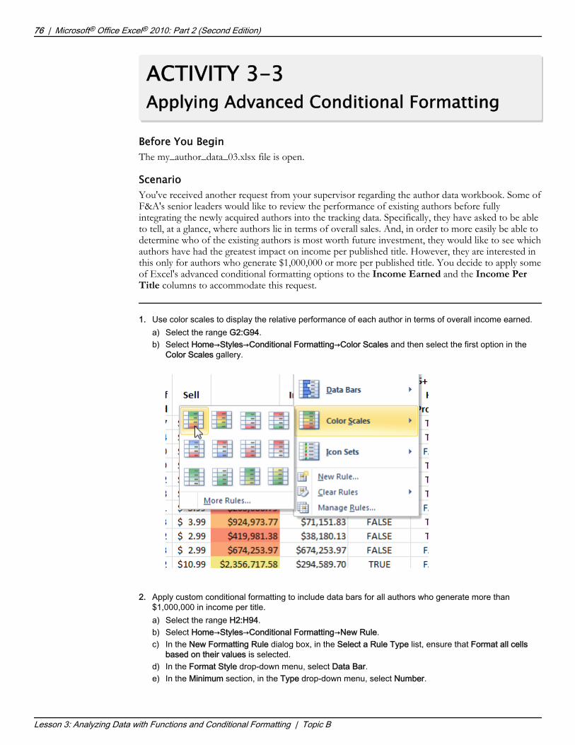
ACTIVITY 3-3Applying Advanced Conditional Formatting

Before You BeginThe my_author_data_03.xlsx file is open.

ScenarioYou've received another request from your supervisor regarding the author data workbook. Some ofF&A's senior leaders would like to review the performance of existing authors before fullyintegrating the newly acquired authors into the tracking data. Specifically, they have asked to be ableto tell, at a glance, where authors lie in terms of overall sales. And, in order to more easily be able todetermine who of the existing authors is most worth future investment, they would like to see whichauthors have had the greatest impact on income per published title. However, they are interested inthis only for authors who generate $1,000,000 or more per published title. You decide to apply someof Excel's advanced conditional formatting options to the Income Earned and the Income PerTitle columns to accommodate this request.

1. Use color scales to display the relative performance of each author in terms of overall income earned.a) Select the range G2:G94.b) Select Home→Styles→Conditional Formatting→Color Scales and then select the first option in the

Color Scales gallery.

2. Apply custom conditional formatting to include data bars for all authors who generate more than$1,000,000 in income per title.a) Select the range H2:H94.b) Select Home→Styles→Conditional Formatting→New Rule.c) In the New Formatting Rule dialog box, in the Select a Rule Type list, ensure that Format all cells

based on their values is selected.d) In the Format Style drop-down menu, select Data Bar.e) In the Minimum section, in the Type drop-down menu, select Number.



Do Not D

uplicate

or Dist

ribute

f) In the Value field, type 1000000g) In the Maximum section, ensure that Automatic is selected in the Type drop-down menu.h) In the Bar Appearance section, select the Color down arrow and, from the Standard Colors section

of the Color gallery, select Red.

i) Select OK.

3. Select any cell to deselect the range H2:H94 and scroll through the worksheet to review the authors'performance.




Do Not D

uplicate

or Dist

ribute

SummaryIn this lesson, you analyzed data by using text and logical functions, and you applied advancedconditional formatting to a worksheet. Making the transition from using Excel as a data storage toolthat performs basic calculations to using it as a tool to extract critical organizational intelligencefrom your raw data is a major milestone in your development as an Excel user. The ability to askquestions of your data by using the appropriate functions and to display the results in an easilydigestible manner are the cornerstones of providing your organizational leaders with the intelligencethey need to give you a competitive edge in today's market.

How will the ability to use logical functions change the way you use Excel?

A: Answers will vary, but many students view the ability to use logical functions as the bridge betweenusing Excel to perform calculations and using it to perform data analysis.

What tasks will Excel's advanced conditional formatting options make easier for you in your current role?

A: Answers will vary, largely depending on the student's role and organization. Some users will find ituseful to be able to easily display overall data patterns to a general audience. Others will likely useconditional formatting to search for and identify anomalies in their data that could affect calculationaccuracy for critical computations. Some users may find the ability to apply multiple rules to the samedataset helpful when looking to assign resources to particular issues or projects, or to identifypersonnel who require various levels of training or support.



Lesson 3: Analyzing Data with Functions and Conditional Formatting |


Do Not D

uplicate

or Dist

ribute

Organizing andAnalyzing Datasets andTablesLesson Time: 2 hours

Lesson ObjectivesIn this lesson, you will organize and analyze datasets and tables. You will:

• Create and modify tables.

• Sort data.

• Filter data.

• Use the SUBTOTAL and database functions.

Lesson IntroductionUsing formulas and functions to analyze data is a powerful way to get a handle on what'sreally going on in your organization. But you may not always need to analyze all of the datapresent in your workbooks. Perhaps you're looking for answers to questions regarding onlya specific set of data. In extremely large workbooks, applying functions to or reviewing theresults of calculations for thousands of rows and columns of data can be a tedious anderror-prone process. Your data is most useful when it's presented in a concise, easy-to-digestfashion. Organizational leaders will want to review and consider only the most relevant data.You'll need a way to pare down massive volumes of data to present only the informationthat is truly important.This is why Excel 2010 provides you with a number of options for ordering and condensingyour data according to a variety of criteria. Taking advantage of this type of functionalitywill save you time and effort, make your analyzed or raw data easier to review, and alloworganizational leaders to focus their efforts on the most important issues.

4

Do Not D

uplicate

or Dist

ribute

TOPIC ACreate and Modify TablesWhen you need to analyze or review a massive amount of worksheet data, you want to be able toisolate pertinent data as quickly and as easily as possible. One huge advantage would be the ability totreat all of your data as a single chunk of entries paired with the ability to hone in on only the datayou need to analyze. Of course, you don't want any of this to disrupt your raw data, as you'll likelyneed to come back later and focus on something else. Excel 2010 contains a very powerful elementof functionality that lets you do all of this in its tables feature.By converting your raw or analyzed data into tables, you'll be able to leverage Excel's incrediblypowerful organizational capabilities without affecting any of the data you've entered into yourworksheets. You'll be able to hone in on specific bits of information, regardless of how many entriesyour worksheets contain. Understanding how all of this works and being able to focus in on just thecritical bits of information in your worksheets will give you a huge advantage when it comes tomining your data to get the right people the precise information they need to act in a competitive,fast-changing world.

TablesIn Excel, a table is simply a dataset composed of contiguous rows and columns that Excel treats as asingle, independent object. Excel tables contain a robust set of functionality that allows you toorganize, change the display of, and perform calculations on worksheet data with just a few mouseclicks. Regardless of how many ways you manipulate your table data, the raw data you initiallyentered remains intact. You can create tables from existing ranges, or create empty tables, and thenpopulate them. You can also revert tables back to simple ranges.As with cells and ranges, you can apply defined names to tables for ease of reference. When youcreate a table, Excel automatically assigns it a generic name, such as Table1 or Table2, but you canchange these to suit your needs. You can also expand existing tables to accommodate additional dataand you can insert or delete columns and rows within tables just as you can in a range.

Note: Named tables must adhere to the same naming conventions as other named elements.

Figure 4-1: Data in an Excel table.


Lesson 4: Organizing and Analyzing Datasets and Tables | Topic A

Tables

Do Not D

uplicate

or Dist

ribute

Table ComponentsThere is a basic set of table components that Excel tables can contain, but don't necessarily have to.By default, Excel tables contain a header row and appear with banded rows. You can toggle thedisplay of these and other components on or off to suit your needs and to provide access to orsuppress various functionality.

Figure 4-2: An Excel table with all of the components displayed.

The following table describes the various components of Excel tables and their functions.

Excel Table Component Description

Header row Displays column headers for the table and provides you with accessto some of Excel's table-organization functionality.

Header row down arrow Displays a drop-down menu that provides you with access tocommands you can use to organize and change the display of yourtable data.

Total row Displays the results of column-specific calculations and provides youwith access to some of Excel's built-in table-function capabilities.

Total row down arrow Displays a drop-down menu that provides you with quick and easyaccess to functions for performing calculations on table-column data.

Banded rows These make it easier to view individual rows of data by applyingdifferent formating to alternating table rows.

Banded columns These make it easier to view individual columns of data by applyingdifferent formatting to alternating table columns.

First column Sets off the display of the first column of data by applying specificformatting, typically bolding, to it.

Last column Sets off the display of the last column of data by applying specificformatting, typically bolding, to it.



Table Components

Do Not D

uplicate

or Dist

ribute

The Create Table Dialog BoxYou can use the Create Table dialog box to convert simple ranges of data into tables. From here,you can confirm the range selection you wish to convert into a table or modify that range to ensurethat the correct data becomes part of the table. The Create Table dialog box also enables you todecide whether or not you wish to include the top row of the selected range in the new table as aheader row. Typically, you would do this if the selected range contains column labels in the top row.You can access the Create Table dialog box by selecting Insert→Tables→Table.

Figure 4-3: Use the Create Table dialog box to convert raw data into a table.

The Table Tools Contextual TabThe Table Tools contextual tab contains various commands and options that are specific toworking with tables. It appears when you select a worksheet table, or any part of a table, anddisappears when you select an object outside the table. The Table Tools contextual tab containsonly one tab, the Design tab, which is divided into five command groups.

Figure 4-4: The Table Tools contextual tab.

The following table identifies the types of commands and options contained in the various groupson the Table Tools contextual tab.

Table Tools Contextual Tab Group Contains Commands or Options For

Properties Resizing worksheet tables. This group also displays the nameof the currently selected table.

Tools Removing duplicate values from tables, converting tablesback into ranges, and creating PivotTables out of tables.

External Table Data Exporting table data to external applications and managingdata links with external sources.

Table Style Options Toggling the display of table components on or off.

Table Styles Applying styles to Excel tables.

Table Styles and Quick StylesLike cell styles, table styles are particular configurations of formatting options you can apply to yourworksheet tables. Table styles help make your tables more visually appealing and easier to read.Table styles can consist of font, border, and fill formatting, and you can create your own customized



The Create Table DialogBox

The Table ToolsContextual Tab

Table Styles and QuickStyles

Do Not D

uplicate

or Dist

ribute

table styles or select from among a variety of pre-configured table styles, which are known as quickstyles.

Figure 4-5: A highly stylized Excel table.

The New Table Quick Style Dialog BoxYou will use the New Table Quick Style dialog box to create and save custom table styles. Fromhere, you can select which table component you wish to apply formatting to; access the FormatCells dialog box to configure the desired font, border, and fill formatting; and name and save yourcustom quick styles. To access the New Table Quick Style dialog box, on the Design tab of theTable Tools contextual tab, in the Table Styles group, select the Table Styles gallery's Morebutton, and then select New Table Style.



The New Table QuickStyle Dialog Box

Do Not D

uplicate

or Dist

ribute

Figure 4-6: The New Table Quick Style dialog box.

Access the Checklist tile on your LogicalCHOICE course screen for referenceinformation and job aids on How to Create and Modify Tables.



Do Not D

uplicate

or Dist

ribute

ACTIVITY 4-1Creating and Modifying a Table

Data FileC:\091019Data\Organizing and Analyzing Datasets and Tables\author_data_04.xlsx


ScenarioBecause Fuller and Ackerman (F&A) acquired two new publishing houses, the author dataworksheet has grown considerably in size. You have finished merging all new authors and their datainto the workbook, and you have added royalty rate information. As you now have to perform dataanalysis on a much larger dataset, you decide it would be in your best interest to convert the rangeon the Authors worksheet into a table. You also decide to define a name for the table to make iteasier to reference for future data analysis and to apply a table style to the table to better adhere toF&A branding guidelines.

1. Open the author_data_04.xlsx workbook file and ensure that the Authors worksheet is selected.

2. Convert the dataset into a table.a) Select any cell within the dataset.b) Select Insert→Tables→Table.c) In the Create Table dialog box, in the Where is the data for your table? field, verify that =$A$1:$K

$1074 is the displayed range.d) Ensure that the My table has headers check box is checked and select OK.e) Adjust the column widths as needed so the header row down arrows do not block any of the column

header text.

3. Apply a quick style to the table.a) If necessary, select any cell within the table to display the Table Tools contextual tab.

b) Select Design→Table Styles and select the Table Styles gallery More button.



The multi-cell arrayformula has beenremoved from thedataset in theauthor_data_04.xlsxworkbook file because itcan't be included in atable. The calculationshave been pasted backinto the cells as valuesto facilitate this activity.

Do Not D

uplicate

or Dist

ribute

c) In the Table Styles gallery, in the Medium section, select the Table Style Medium 11 quick style.

4. Create a defined name for the table.a) From the Table Tools contextual tab, in the Properties group, in the Table Name field, type

Table_Author_Totalsb) Press Enter.

5. Verify Excel created the table name.a) Select Formulas→Defined Names→Name Manager.b) In the Name Manager dialog box, ensure that Table_Author_Totals appears in the list of defined

names, and that it refers to the range $A$2:$K$1074.c) Close the Name Manager dialog box.

6. Save the workbook to the C:\091019Data\Organizing and Analyzing Datasets and Tables folder asmy_author_data_04.xlsx



Inform students theymay have to adjust thecolumn widths in theName Manager dialogbox to view all of theinformation for step 5b.

Do Not D

uplicate

or Dist

ribute

TOPIC BSort DataRaw data is often entered into Excel worksheets in random order, or at least not in the order youneed for a particular data analysis task. For example, sales data may be entered chronologically, butyou may need to examine information related to particular products or store locations. Or, you needto review employee data based on hire date, but the entries are listed alphabetically by employee lastname. Scouring large worksheets to pick out the necessary entries is tedious, time consuming, andprone to errors. Wouldn't it be easier if you could rearrange your data to help you review only thoseentries that apply to the task at hand? In Excel, rearranging your data based on particular criteria isstraightforward.By reordering your data, you can more easily locate and interact with specific entries, even inmassive worksheets with tens of thousands of entries. In essence, you can provide yourself with aroadmap to get to your destination without having to take a bunch of wrong turns. Placing your datain the proper order will save you time and a few headaches, and will ensure the information you'rereporting to organizational leaders contains minimal amounts of errors.

SortingSorting is, quite simply, reordering the data in your worksheets based on some defined criteria, suchas alphabetically or from highest value to lowest value. Sorting allows you to put data entries in asequence that makes sense for a particular task. In Excel, you can sort by row or column, but anoverwhelming majoring of sorting is done by column because of the way most people enterworksheet data. You can sort on a single row or column or apply multiple sorts to the same set ofdata. You can sort either range or table data. Excel can sort data based on a number of differentvalues, such as numeric, alphabetical, date and time, and even by cell color or conditional formattingcriteria. If you add data to a sorted range or table, you can re-sort to accommodate the new entries.It is important to keep in mind that when you sort data, you are not changing the data in yourworksheets. You are merely changing the display of the data. So, while you may sort on oneparticular column in a worksheet, say by numeric value, after the sort, each entry (individual row)will have the same data across the entire row. The rows will just appear in a different order based onthe sort criteria. This preserving of data integrity is what makes sorting a powerful, useful feature.

Note: It's a best practice to select only a single cell within a column or row when sorting. Whenyou do this, Excel will automatically preserve the integrity of your data as described previously.However, if you select an entire column or row and then sort, Excel prompts you to include thesurrounding data in the sort. If you do not expand the selection to include the surrounding data,your data integrity will not be maintained.

There are a couple of things about sorting that you should keep in mind. First, you cannot clearsorting, but you can use the Undo command to revert sorted data back to its previous state. Second,when you save and close workbook files, you save sorts along with it. So if you want to undo a sort,you must do it before saving and closing the file or before performing more actions than your undosettings allow you to undo. You can access the sort commands in the Sort & Filter group on theData tab.


Lesson 4: Organizing and Analyzing Datasets and Tables | Topic B

Sorting

Do Not D

uplicate

or Dist

ribute

Figure 4-7: The same Excel worksheet both unsorted and sorted.

Multiple Column/Row SortingWhen you sort on multiple columns or rows, it's important to consider that all of the columns orrows on which you're sorting, except for the last one you sort on, should contain some duplicateentries. Otherwise, the sort is of no value. Consider the simple example in the following figure.

Figure 4-8: Sorting on multiple columns or rows enables you to organize your data inincreasingly meaningful ways.



Multiple Column/RowSorting

Do Not D

uplicate

or Dist

ribute

In this example, the dataset is sorted in ascending order on three different columns. First, it is sortedby the number of titles in print, then by sell price, and finally by the number of books sold. This sortcan provide some analytical value because there are multiple entries with duplicate values in the firsttwo columns the data is sorted on. For example, of all of the authors with only one title in print,four of them also have books that sell for $2.99. Because of this, there is a meaningful sort on thevalues in the Number of Books Sold column.

Quick SortsThere are two general categories of sorting in Excel: quick sorts and custom sorts. Quick sorts enableyou to easily sort the data in a range or table according a set of predefined criteria. Although tableshave quick sorting functionality built into them, for ranges, by default, you need to use commandson the ribbon. By using quick sorts, you can sort data one column at a time, in ascending ordescending order, according to the type of content stored in the column. So, for example, if thecolumn contains text, you can sort by alphabetical order. If the cells contain numeric values, you cansort lowest to highest or highest to lowest. If the cells contain dates, you can sort based onchronological order. With quick sorts, you can sort only by column, not by row.

Note: Although tables have built-in sorting capabilities, you can sort them by using ribboncommands as well.

Figure 4-9: Use quick sorts to easily reorder your range or table data.

Custom SortsTo sort your range or table data by using more highly defined criteria than is possible by using quicksorts, you can define a custom sort. Custom sorting enables you to sort by row or column, sort onmultiple rows or columns simultaneously, and to define specific sort criteria. In addition to the sortcriteria that is available by using quick sorts, custom sorts allow you to sort based on cell and fontcolor, and based on conditional formatting icons.Each specific criterion you assign to a custom sort is called a level. Excel evaluates and sorts yourdata based on the order in which you assign sort levels to the data. You can add, delete, edit, andreorder sort levels. Custom sorting is only possible by using ribbon commands.

Note: You cannot apply both column and row sorting to the same data range. Also, you cannotsort tables by row.



Quick SortsAlthough users canaccess quick sortingoptions for data rangeswhen filtering is turnedon, that is not mentionedhere. This is becausefiltering isn't introduceduntil the next topic. Thisfunctionality will beaddressed there.

Do Not D

uplicate

or Dist

ribute

The Sort Dialog boxYou use the Sort dialog box to define and manage your custom sorts. You can access the Sortdialog box by selecting Data→Sort & Filer→Sort.

Figure 4-10: The Sort dialog box displaying multiple sort levels for a data range.

The following table describes the functions of the various Sort dialog box elements.

Sort Dialog Box Element Description

Add Level button Adds new blank sort levels to a custom sort.

Delete Level button Removes the currently selected sort level from a customsort.

Copy Level button Creates a copy of the currently selected sort level and placesit immediately after the selected level.

Move Up/Move Down buttons Allow you to reorder the sort levels in a custom sort.

Options button Opens the Sort Options dialog box.

Column/Row Sort by drop-downmenu

Use this to select the column or the row upon which tosort your data. Setting your sort options determineswhether you sort by row or column.

Sort On drop-down menu Use this to select the criteria by which you want to sortyour data.

Order drop-down menu Use this to determine the order in which Excel will displaysorted data, for example, alphabetical or oldest to newest.The options that the Order drop-down menu displaysdepend on the selections you make in the Column/RowSort by drop-down menu and the Sort On drop-downmenu.

Custom sort levels The sort levels appear in the order in which Excel willevaluate and apply data sorting.

The Sort Options Dialog BoxYou use the Sort Options dialog box to determine whether Excel will sort by column or row and todefine the precedence Excel applies to capitalization while sorting. When the Case sensitive checkbox is unchecked, Excel gives precedence to capital letters. When the Case sensitive check box is



The Sort Dialog Box

The Sort Options DialogBox

Do Not D

uplicate

or Dist

ribute

checked, it gives precedence to lowercase letters. You can access the Sort Options dialog box byselecting the Options button in the Sort dialog box.

Figure 4-11: Use the Sort Options dialog box to assign sorts to rows or columns and to definethe precedence Excel applies to capitalization.

Access the Checklist tile on your LogicalCHOICE course screen for referenceinformation and job aids on How to Sort Data.



Do Not D

uplicate

or Dist

ribute

ACTIVITY 4-2Sorting Data

Before You BeginThe my_author_data_04.xlsx file is open.

ScenarioYou have been asked to create several reports for company senior leaders for an upcoming meeting.While preparing to create these reports, you notice a few issues in the author data. Specifically, thereare several authors who have a negative value in the Years Under Contract column, and there are anumber of author IDs that appear more than once. You realize that this could be a serious issue, soyou consult with a colleague in the HR department and discover that some of the data wascorrupted during the author-integration process.In consultation with HR, you have decided to remove all author entries for authors with a negativevalue for years under contract and to remove duplicate author ID records. Your colleague in HR hasindicated that, for any duplicate author IDs, the oldest record is the valid record.

1. Sort the dataset from highest to lowest on the Income Earned column.

a) In cell G1, select the column header down arrow and then select Sort Largest to Smallest.b) Scroll down slightly and verify that there are several negative values in cells in the Years Under

Contract column.

Note: The purpose of this first sort is to simply bring some of the negativevalues into view. The next sort will arrange the table so you can delete theundesired entries.

2. Delete all entries for authors with a negative value in the Years Under Contract column.a) In cell C1, select the column header down arrow and then select Sort Smallest to Largest.b) Select the range C2:C40.



This is a goodopportunity to ask thestudents why all of thevisible cells in theIncome Earned columnare now green.(Because the table issorted on that column,all of the highest valuesappear first.)

Do Not D

uplicate

or Dist

ribute

c) Right-click the selected range and then select Delete→Table Rows.

d) Verify that author 1989 is now the first author listed in the table.

3. Sort the table by two columns simultaneously.a) Select any cell within the table and then select Data→Sort & Filter→Sort.b) In the Sort dialog box, in the Sort by section, from the Column drop-down menu, select AuthorID.c) Ensure that Values is selected in the Sort On drop-down menu.d) Ensure that Smallest to Largest is selected in the Order drop-down menu.e) Select Add Level to add another sort level.f) In the Then by section, from the Column drop-down menu, select Initial Contract Date.g) In the Sort On drop-down menu, ensure that Values is selected.h) In the Order drop-down menu, ensure that Oldest to Newest is selected.

i) Select OK.

4. Highlight the duplicate author ID records to verify the sort worked as expected.a) Select the range A2:A1035.b) Select Home→Styles→Conditional Formatting→Highlight Cells Rules→Duplicate Values.c) In the Duplicate Values dialog box, in the values with drop-down menu, select Yellow Fill with Dark

Yellow Text.d) Select OK.e) Scroll to the top of the worksheet until the range A18:A21 is visible.



Do Not D

uplicate

or Dist

ribute

f) Verify that the entries for rows 18-21 all contain duplicate values and that they appear inchronological order.

5. Remove the duplicate records.

a) Select Data→Data Tools→Remove Duplicates.

Note: The Remove Duplicates command works by deleting all but the firstlisted duplicate record. This is why you first sorted by author ID, and thensorted by initial contract date. The records Excel will retain will be the earliestof each of the duplicates.

b) In the Remove Duplicates dialog box, select Unselect All.c) Check the Author ID check box.d) Select OK.e) In the Microsoft Excel dialog box, verify that Excel deleted 222 duplicate records and then select

OK.




The students will beusing the RemoveDuplicates command inthis activity, which maybe new to them.Students at this levelshould have no issueswith this feature, but beprepared to assistanyone having difficulty.Proactively reach out toremote students tomonitor their progress.

Do Not D

uplicate

or Dist

ribute

TOPIC CFilter DataImagine if you will, you're standing in a field in front of a haystack and a bucket. Somewhere in thehaystack is the proverbial needle; in the bucket, there is a baseball and a bunch of marbles. Your jobis to locate either the needle or the baseball. Given the choice, which would you rather look for?Now, apply this metaphor to analyzing data in large worksheets. Though sorting can help you locateand review data in large worksheets, it does nothing to cut down on the number of displayed entries.Even with ordered data, you may often still need to sift through large volumes of data, which can bechallenging and time consuming. Clearly, it would be far more efficient to review only the data thatis absolutely essential to the task at hand. The Excel 2010 filtering feature helps you do exactly that.By reducing the volume of data entries you need to review and analyze, you cut out extraneous andwasted effort. Paring down massive volumes of data into a small handful of pertinent, useful entrieswill make your data analysis and reporting tasks faster, easier, and more accurate than they would beif you had to deal with irrelevant entries.

FilteringAs with the sorting feature, you can use the filtering feature to make data far easier to work with.Whereas sorting merely rearranges your data based on particular defined criteria, filtering removesfrom view any data entries that do not match the specified criteria. When you filter data in Excel,you do not affect the actual data entries. You alter only how Excel displays your data. It is importantto note that filtering affects entire worksheet rows. If you have data in a range or a table next to datathat you filter, rows that are suppressed from view in the data you're filtering are also suppressedfrom view in the adjacent tables or ranges.You can filter both tables and data ranges in Excel, and you can filter on more than one column.However, you can filter only by column and not by row. You can combine sorting and filtering tofine tune the display of your data. Typically, when you combine sorting and filtering, it's a bestpractice to filter first and then sort just the data you wish to work with. Filtering functionality isactive in tables by default, but you must turn it on for data ranges. You can toggle filtering on andoff for both ranges and tables. To toggle filtering on and off for tables or ranges, select any cellwithin the desired table or range and select Data→Sort & Filter→Filter.

Note: When you turn on filtering for a data range, you also activate quick sorting functionalityfor the range. In essence, you give it much of the same functionality that tables have, but withoutthe total row and formatting functionality. Be sure that you select either only a single cell withinthe range or the entire data range when turning on filtering for a range. If you select only certaincolumns within a range when turning on filtering, when you use quick sorts to sort the range,columns not included in the selection when you turned on filtering will not sort with the rest ofthe data.

Unlike sorting, filtering can be cleared at any time to re-display all rows that the filtering temporarilysuppressed. When you apply functions to or search filtered data, Excel applies the function to orsearches through only the data that is displayed. When you clear filters, Excel applies the function toor searches through the entire dataset.

Caution: Filtering data and hiding rows or columns can have a wide range of effects on the Cutand Copy commands. When cutting or copying and then pasting data from filtered datasets ordatasets with hidden columns or rows, always ensure that your pasted values appear as expected.


Lesson 4: Organizing and Analyzing Datasets and Tables | Topic C

Filtering

Do Not D

uplicate

or Dist

ribute

Figure 4-12: Filtering data removes all non-pertinent entries from view, making it easier toreview and work with your data.

AutoFiltersAutoFilters enable you to quickly filter datasets and tables based on unique cell entries or applied cellformatting in a column. AutoFilter options appear in two ways: as check boxes or as pop-up menuoptions in the header row drop-down menu of tables or ranges that have filtering turned on. Youuse the list of check boxes to filter based on cell values. Checked items will appear in the filtereddataset, unchecked items will not. You can check or uncheck any number of entries for eachcolumn, and you can search for specific entry values to pare down the list of AutoFilter options.The search functionality for AutoFilter values is dynamic, so Excel filters the AutoFilter options asyou type each character of your search term.You use the pop-up menu options to filter cells based on font or fill color, or based on icon sets.Again, for whichever formatting criteria you select in the pop-up menu, Excel will display rowscontaining that particular formatting; all other rows are hidden. You can use AutoFilters to filterblended criteria. In other words, you can filter by cell value and by formatting in the same columnbut you can filter based on only one formatting criteria at a time.The AutoFilter feature is most useful in columns that contain multiple duplicate entries orformatting options. Excel will display only one check box for each unique data entry (up to 10,000unique values) in the column and one formatting option for each unique formatting element.Columns that you have applied filtering to will display a slightly different header row down arrow.

For unfiltered columns, the header row down arrow appears like this ; in filtered columns, it

looks like this.



AutoFilters

Do Not D

uplicate

or Dist

ribute

Figure 4-13: AutoFilters enable you to quickly filter datasets based on unique column entries.

Custom AutoFiltersIn addition to using the default AutoFilters available in Excel, you can customize AutoFilters tofilter datasets by specific criteria. You can use custom AutoFilters to filter by such criteria as aparticular range of numeric values, text entries that begin with a particular character, or all entriesmade before or after a particular date. The custom AutoFilter options available to you depend onthe type of data stored in the column. You can access these options by selecting either Text Filters,Number Filters, or Date Filters from the header row drop-down menu of ranges or tables thathave filtering turned on. Selecting any of these options from the drop-down menu opens asecondary menu. In the secondary menu, some of the filter options have no configurableparameters, such as filtering for the top or bottom 10 percent of numerical values, so selecting themwill simply apply the filter. Others do need to be configured, so, when you select them, Excel opensthe Custom AutoFilters dialog box.

The Custom AutoFilter Dialog BoxYou use the Custom AutoFilter dialog box to configure the parameters for some of Excel's customAutoFilters. The options available in the Custom AutoFilter dialog box vary depending on the typeof data in the column. You can set one or two parameters in the Custom AutoFilter dialog box.For example, if you'd like to filter for a certain range of numeric values, you would enter the top andbottom values of the desired range. You can also select whether Excel should filter data based onentries that meet both defined criteria or based on meeting only one of the two criteria. If you don'tenter a value in the lower fields, Excel ignores them.



The Custom AutoFilterDialog Box

Do Not D

uplicate

or Dist

ribute

Figure 4-14: Use the Custom AutoFilter dialog box to set the parameters for custom AutoFilters.

The following table describes the function of the various elements of the Custom AutoFilter dialogbox.

Custom AutoFilter Dialog BoxElement

Allow You To

Filter selection drop-down menus Select the specific custom AutoFilters you wish to apply toyour dataset. Typically, Excel automatically populates thetop menu with the filter you selected to open the CustomAutoFilter dialog box.

And/Or radio buttons Choose between requiring both filter parameters orapplying the filter to entries matching either one or theother.

Parameter entry text fields/drop-down menus

Define the specific criteria for the search. You canmanually type the entries or select them from the drop-down menu, which is populated with the column's dataentries.

Advanced FilteringExcel's built-in AutoFilter functionality is a fast and easy way to pare down large volumes of datainto manageable, easy-to-view chunks. However, there will likely be times when you will need tofilter your data based on much more complex criteria than the AutoFilter options can support. Inthese cases, you can create advanced filters. When you filter data by using Excel's Advancedfiltering command, you enter filter criteria directly on the worksheet containing the dataset you wantto filter. Advanced filtering uses a set of filter operators that are similar to Excel's logical operators.Although you can filter the original dataset in its original location, you can also ask Excel to returnthe filtered dataset in a different location within the workbook. This provides you with both anunfiltered and a filtered view of your data simultaneously. You can access the Advanced filtercommand by selecting Data→Sort & Filter→Advanced.

Note: Applying advanced filtering to a range or a table with filtering (AutoFilter) turned onautomatically turns off filtering.



Advanced Filtering

Do Not D

uplicate

or Dist

ribute

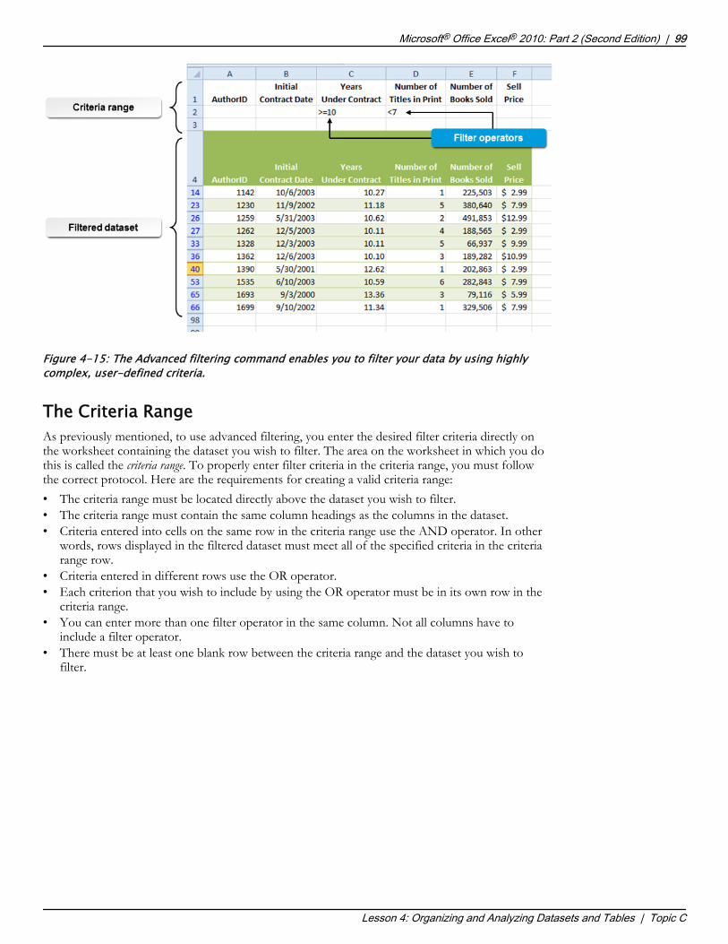
Figure 4-15: The Advanced filtering command enables you to filter your data by using highlycomplex, user-defined criteria.

The Criteria RangeAs previously mentioned, to use advanced filtering, you enter the desired filter criteria directly onthe worksheet containing the dataset you wish to filter. The area on the worksheet in which you dothis is called the criteria range. To properly enter filter criteria in the criteria range, you must followthe correct protocol. Here are the requirements for creating a valid criteria range:• The criteria range must be located directly above the dataset you wish to filter.• The criteria range must contain the same column headings as the columns in the dataset.• Criteria entered into cells on the same row in the criteria range use the AND operator. In other

words, rows displayed in the filtered dataset must meet all of the specified criteria in the criteriarange row.

• Criteria entered in different rows use the OR operator.• Each criterion that you wish to include by using the OR operator must be in its own row in the

criteria range.• You can enter more than one filter operator in the same column. Not all columns have to

include a filter operator.• There must be at least one blank row between the criteria range and the dataset you wish to

filter.



The Criteria Range

Do Not D

uplicate

or Dist

ribute

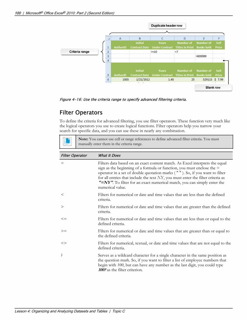
Figure 4-16: Use the criteria range to specify advanced filtering criteria.

Filter OperatorsTo define the criteria for advanced filtering, you use filter operators. These function very much likethe logical operators you use to create logical functions. Filter operators help you narrow yoursearch for specific data, and you can use these in nearly any combination.

Note: You cannot use cell or range references to define advanced filter criteria. You mustmanually enter them in the criteria range.

Filter Operator What It Does

= Filters data based on an exact content match. As Excel interprets the equalsign as the beginning of a formula or function, you must enclose the =operator in a set of double quotation marks ( " " ). So, if you want to filterfor all entries that include the text NY, you must enter the filter criteria as"=NY". To filter for an exact numerical match, you can simply enter thenumerical value.

< Filters for numerical or date and time values that are less than the definedcriteria.

> Filters for numerical or date and time values that are greater than the definedcriteria.

<= Filters for numerical or date and time values that are less than or equal to thedefined criteria.

>= Filters for numerical or date and time values that are greater than or equal tothe defined criteria.

<> Filters for numerical, textual, or date and time values that are not equal to thedefined criteria.

? Serves as a wildcard character for a single character in the same position asthe question mark. So, if you want to filter a list of employee numbers thatbegin with 100, but can have any number as the last digit, you could type100? as the filter criterion.



Filter Operators

Do Not D

uplicate

or Dist

ribute

Filter Operator What It Does* Serves as a wildcard character for multiple characters in the same position as

the asterisk. So, if you want to filter a list of product names for entries thatbegin with the letter S and end with the letter L, you could enter "=S*L" asthe criterion. In this case, both sail and stool would appear in the filtereddataset.

Access the Checklist tile on your LogicalCHOICE course screen for referenceinformation and job aids on How to Filter Data.



Do Not D

uplicate

or Dist

ribute

ACTIVITY 4-3Filtering Data

Before You BeginThe my_author_data_04.xlsx workbook file is open.

ScenarioNow that you have resolved the data errors, you're ready to apply filters to the dataset to answerquestions from company senior leaders to include in your report. These are the questions they haveasked:• How many titles that sell at the highest price are currently in publication?• Who are the top five authors by income earned?• How many authors have been with the company for one year or less?• Which authors have been with the company for fewer than five years and have sold 500,000 or

more books?

1. Use an AutoFilter to answer the question "How many titles that sell at the highest price are currently inpublication?"a) In cell F1, select the column header down arrow.b) Uncheck the Select All check box.c) Check the $23.99 check box and select OK.d) Scroll to the bottom of the table.e) Ensure that any cell in the table is selected, and then display the tables total row by checking the

Total Row check box in the Table Style Options group on the Table Tools contextual tab.f) Select cell F814 and then select the total row down arrow.

g) From the drop-down menu, select Count.

2. How many titles sell at the highest price?A: 43

3. Scroll to the top of the table, select the column header down arrow in cell F1, and then select ClearFilter From "Sell Price."

4. Use an AutoFilter to answer the question "Who are the top five authors by income earned?"a) In cell G1, select the column header down arrow.b) Select Number Filters→Top 10.c) In the Top 10 AutoFilter dialog box, in the Show section, set the value in the spin box to 5.d) Select OK.e) Review the author IDs to determine the top five authors.f) Clear the filter from the Income Earned column.



Inform students they canjust ignore the figure thatappears in cell K814. Bydefault, Excel assumesthe last column in a tableis a total column andautomatically sums thevalues in it.If students ask aboutusing the built-infunctions in the total row,let them know that this isa "sneak peek" at howthese work, and that thisfunctionality is coveredin depth in the nexttopic.

Do Not D

uplicate

or Dist

ribute

5. Use advanced filtering to answer the question "How many authors have been with the company for oneyear or less?"

a) Insert three empty rows above the table's header row.

b) Copy and paste all of the table's column headers into the top row directly above the existing

headers.

c) In cell C2, type <=1 and then press Enter.d) Select any cell within the table and then select Data→Sort & Filter→Advanced.e) In the Advanced Filter dialog box, in the List range field, verify that $A$4:$K$816 appears.f) In the Criteria range field, select the Collapse Dialog button, select the range A1:K2 on the

worksheet, and then press Enter.g) Select OK.

Note: Remember that using advanced filtering automatically turns off thetable's built-in filtering functionality. You can turn this back on by selectingData→Sort & Filter→Filter.



If students don'tremember how to insertrows at the top of aworksheet, remind themto select the entire firstrow, right-click theselection, and selectInsert. They can thenpress F4 twice to repeatthe action two moretimes.

Although the screenimage here displays onlysome of the headers,inform students that theymust copy and paste allof the headers above thetable.

Do Not D

uplicate

or Dist

ribute

h) Scroll to the bottom of the table.

6. Does the COUNT function result in the Sell Price column answer the question "How many authors havebeen with the company for one year or less?"A: Yes, the COUNT function in any of the total row cells would give the correct answer. A total of 48

authors have been with the company one year or less.

7. Select Data→Sort & Filter→Clear to clear the filter.

8. Scroll to the top of the table and delete the filter operator in cell C2.

9. Use advanced filtering to answer the question "Which authors have been with the company for fewerthan five years and have sold 500,000 or more books?"a) If necessary, re-select cell C2, type <5 and then press Tab twice.b) Ensure that cell E2 is selected, type >=500000 and then press Enter.c) Select any cell within the table and then select Data→Sort & Filer→Advanced.d) In the Advanced Filter dialog box, in the List range field, change the entry to $A$4:$K$816e) Ensure that $A$1:$K$2 appears in the Criteria range field.f) Select OK.g) Scroll through the filtered table to confirm the filter worked as planned and to review the author IDs

for the authors who meet these criteria.

10. Select cell F817 and press Delete.

11. Clear the filter and save the workbook.



Let the students knowthat the built-in functionsin the Total row of tablesreflect the currentlyfiltered state of the table.So, in this case, for anyfilter performed, theCOUNT function wouldaccurately count theunfiltered entries.

Do Not D

uplicate

or Dist

ribute

TOPIC DUse SUBTOTAL and Database FunctionsThe ability to sort and filter your data makes sifting through large volumes of entries and applyingcalculations to only particular sets of data fast and easy. But what if you need to perform calculationson a variety of subsets of data at once? For example, let's say your organization has branch officesall over the country. What if you want to find the total or the average sales for the sales reps in eachof these regions? Filtering your data for each region, and then applying functions to the data subsetsbecomes a repetitive, tedious process. This is especially true if your organization is divided into 20 or30 regions. Or, perhaps, you want to analyze the total or average sales for a variety of products orservices at once. If your organization offers thousands of products, this could become a nightmare.And, if you want to perform some type of analysis on a very particular subset of data, one thatmeets incredibly precise criteria, drilling down into your data to perform the calculations couldinvolve a lot of work or be nearly impossible.What all of this means is you're going to need a more efficient, accurate way to drill down into yourdata to analyze it on a granular level. Excel provides you with a number of ways to do this. Themore comfortable you become with Excel's ability to focus on specific, fine detail in massivedatasets, the better able you'll be to ask specific questions and get the answers you need to makesound organizational decisions.

SUBTOTAL FunctionsBefore you look at two key elements of Excel functionality that will help you analyze your data on amore granular level, it will be helpful to look at a different type of Excel function, one that lies at thecore of this functionality: SUBTOTAL functions. SUBTOTAL functions are a specific set of Excelfunctions that perform calculations on a subset of data.

Note: Although it is important to have an understanding of how SUBTOTAL functions work interms of syntax, most users take advantage of them through ribbon commands and other UI-based functionality as opposed to entering them manually by typing.

The most common calculation you will likely make by using SUBTOTAL functions is, notsurprisingly, finding subtotals. Take a look at this example to get a sense of how useful thesefunctions can be.


Lesson 4: Organizing and Analyzing Datasets and Tables | Topic D

If the students ask,inform them that thefocus of much of the restof this topic is on usingSUBTOTAL functionsthrough the ribbon andthe user interface.

Do Not D

uplicate

or Dist

ribute

In this example, a range of sales data has been sorted by region. To find the sales totals by region,we've added extra rows in the worksheet, and used the SUM function to calculate each region's totalsales, which are subtotals of the company's overall sales. This is simple enough to do if you'redealing with a relatively small worksheet, but this could quickly become quite a chore in larger ones.So, having a function that can perform the subtotal calculation on a very large dataset can be quiteadvantageous.Technically speaking, SUBTOTAL functions are not really a group of functions; rather, this is asingle function that calls one other function out of a set of available functions, such as SUM,AVERAGE, MAX, and MIN, depending on the specific calculation you want Excel to perform. Itthen performs the selected function on the range or ranges you stipulate in the arguments. Here isthe function's syntax:=SUBTOTAL(function_num, ref1, [ref2], ..., [ref254])In the function's syntax, the reference arguments, ref1, ref2, and so on, simply tell the functionwhich ranges to perform the calculations on. The function_num argument calls the specificfunction you want to use to calculate your subtotals. You express this argument as a single numericvalue of 1 to 11 or 101 to 111. Of the available functions the SUBTOTAL function can call, thereare two different groups, hence the two sets of possible values for the function_num argument.These are two identical sets of functions: If you enter a value from 1 to 11 as the argument, theselected function will include hidden values (because of hidden rows or columns in your worksheet);if you enter a value from 101 to 111 as the argument, the selected function will ignore hidden values.The following table outlines the functions each value in the function_num argument calls.

Function_num Argument(Includes Hidden Values)

Function_num Argument(Ignores Hidden Values)

Called Function

1 101 AVERAGE

2 102 COUNT

3 103 COUNTA

4 104 MAX

5 105 MIN

6 106 PRODUCT



Do Not D

uplicate

or Dist

ribute

Function_num Argument(Includes Hidden Values)

Function_num Argument(Ignores Hidden Values)

Called Function

7 107 STDEV

8 108 STDEVP

9 109 SUM

10 110 VAR

11 111 VARP

So, if you have a large set of data in column A of a worksheet, and you want the subtotal for thefirst 20 values, you would enter the following function: =SUBTOTAL(9, A1:A20). If you wantedto find the average value of that same range, you would enter =SUBTOTAL(1,A1:A20). If thatrange contained hidden rows that you wanted to ignore while performing the same calculations, youwould use 109 and 101 for the function_num arguments, respectively.

Note: Both sets of SUBTOTAL functions ignore values removed from view because offiltering.

The Subtotals FeatureAs previously mentioned, although it's good to have a grasp of the SUBTOTAL function's syntax, itisn't necessary to manually enter these functions. This is because Excel 2010 includes severalfeatures that enter the appropriate function for you automatically. One of these is the Subtotalsfeature. Selecting the Subtotals command enables you to automatically perform SUBTOTALfunction calculations on subsets of data within a particular dataset. The Subtotals feature does notwork on tables.

Note: Although it is possible to enter SUBTOTAL functions in a table manually, they are ratherdifficult to work with in that environment. It is generally recommended that you convert thetable to a dataset or copy it as a dataset and then use the Subtotals feature.

One of the most important things to remember about the Subtotals feature is that it is mosteffective when you have included column headers in the dataset and you have already sorted yourdata by some specific criteria, for example, region or financial period, for which you wish tocalculate subtotals. This is because the Subtotals feature looks for changes in the column entries ofone column, and then performs the desired calculation on the corresponding values in anothercolumn.



The Subtotals Feature

Do Not D

uplicate

or Dist

ribute

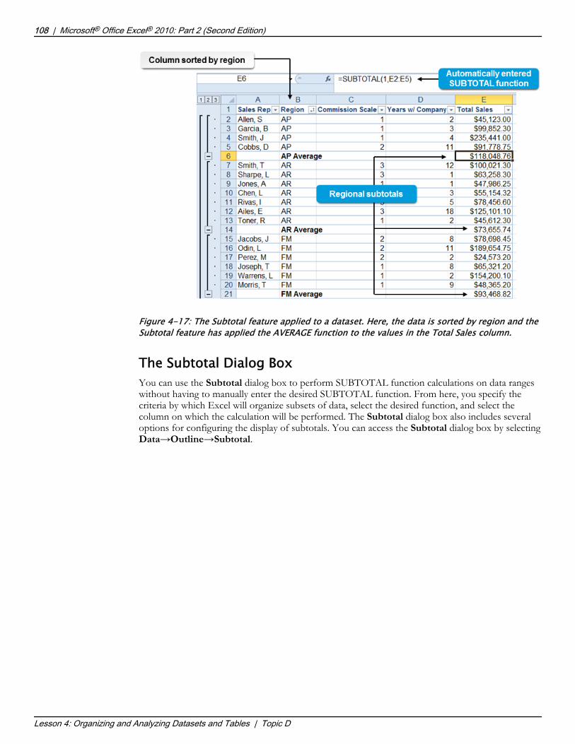
Figure 4-17: The Subtotal feature applied to a dataset. Here, the data is sorted by region and theSubtotal feature has applied the AVERAGE function to the values in the Total Sales column.

The Subtotal Dialog BoxYou can use the Subtotal dialog box to perform SUBTOTAL function calculations on data rangeswithout having to manually enter the desired SUBTOTAL function. From here, you specify thecriteria by which Excel will organize subsets of data, select the desired function, and select thecolumn on which the calculation will be performed. The Subtotal dialog box also includes severaloptions for configuring the display of subtotals. You can access the Subtotal dialog box by selectingData→Outline→Subtotal.



The Subtotal Dialog Box

Do Not D

uplicate

or Dist

ribute

Figure 4-18: Use the Subtotal dialog box to configure your subtotal calculations.

The following table describes the function of the various elements of the Subtotal dialog box.

Subtotal Dialog BoxElement

Allows You To

At each change in drop-down menu

Select the criteria by which to organize subsets of data. You do thisby selecting the column that contains the desired entries. Forexample, you can tell Excel to perform subtotal calculations on dataentries based on a particular region, department, or product.Remember to first sort your data on the column you will select in theAt each change in drop-down menu and then apply the subtotalcalculation.

Use function drop-downmenu

Select the desired SUBTOTAL function.

Add subtotal to menu Select the column on which you wish to perform the calculation.Like the At each change in drop-down menu, this drop-downmenu is populated with the column headers in the selected dataset.

Replace current subtotalscheck box

Decide between replacing existing subtotals with new subtotalcalculations or including multiple subtotals in your dataset.

Page break betweengroups check box

Place a page break after each subtotal so you can print each subset ofdata separately.

Summary below datacheck box

Include a summary row at the bottom of the table. This will includethe grand total from all of the individual subtotals.

Remove All button Clear all subtotals and subsets from the original dataset.

OutlinesYou may have already noticed that when Excel applies subtotal functions to a range of data, itautomatically creates a layered hierarchy of the various data subsets along the left side of theworksheet. This hierarchy is called an outline. In an outline, subtotaled datasets are arranged into



Outlines

Do Not D

uplicate

or Dist

ribute

groups of varying levels of detail that you can expand or collapse depending on how much detailyou want to see. For example, if you want to carefully analyze individual data entries for theworksheet, you would want to expand all levels in the hierarchy so that all populated cells appear inthe worksheet. But if you want to present summary data to your supervisor on a per-region basis,you may want to display only the subtotal rows that contain the summary information.Outlines can contain up to eight levels of detail. Each level is nested within the previous level. Thelevel buttons along the top of the Outline panel allow you to instantly change the view of yourworksheet to display only the summary information of that level. The higher the number of the levelbutton, the more detailed a view of your data you will see. Data subsets are represented in theoutline by square brackets. These brackets display plus and minus buttons that enable you collapseand expand individual data subsets as desired.Although Excel automatically creates outlines in datasets containing subtotals, you can also manuallyorganize your datasets according to your needs. You will find the commands to do this in theOutline group on the Data tab.

Figure 4-19: Outlines enable you to control how much detail is displayed in worksheetscontaining subtotals.

Summary FunctionsSummary functions automatically perform SUBTOTAL function calculations in tables, much as theSubtotals feature does in datasets. But summary functions do not automatically create data subsetsin tables. You can, however, calculate subtotals in tables by applying a summary function and thenfiltering the table to display only the data subset you wish to perform the calculation on.You perform summary function calculations in tables in much the same way as you filter and sortdata in tables. The best way to do this is to include a total row in the desired table and then selectthe desired function from the total row down arrow in the desired column. This returns the result ofthe selected function in the total row of the that column, which includes all displayed values in thecalculation. Once you have applied the function, you can filter the table data to reapply thecalculation to only the desired values. You can also manually type SUBTOTAL functions into anyworksheet cell, referencing the desired table range, if you wish.



Summary Functions

Remind students theywere introduced to thisfunctionality in theprevious activity.Do N

ot Duplic

ate or D

istrib

ute

Figure 4-20: You can automatically apply summary functions to table columns in tables thatcontain total rows.

Access the Checklist tile on your LogicalCHOICE course screen for referenceinformation and job aids on How to Summarize Data with SUBTOTAL and SummaryFunctions.



Do Not D

uplicate

or Dist

ribute

ACTIVITY 4-4Using Subtotals to Summarize Data

Before You BeginThe my_author_data_04.xlsx workbook file is open.

ScenarioYou're on your way to a meeting. You have been asked to report on the total income generated byFuller and Ackerman's authors. But you have also been asked to give detailed information onincome generated by authors at each of the royalty rate levels. Rather than take the time to filter thetable numerous times and recalculate the income totals for each group, you decide to use theSubtotals feature to provide all of the summary information at once. You realize you will have toconvert your table back to a range to do this, but you also suspect you will need the table for futurecalculation. So, you decide to make a copy of the Authors worksheet and convert the table to arange on the worksheet copy. This way, you'll have easy access to your data as both a range and as atable.

1. Make a copy of the Authors worksheet on which to convert the table to a range.a) Right-click the Authors worksheet tab and select Move or Copy.b) In the Move or Copy dialog box, in the Before sheet list, select Statistics.c) Check the Create a copy check box and select OK.d) Rename the Authors(2) worksheet tab to Authors_Range

2. Convert the table on the Authors_Range worksheet to a range.a) Ensure that the Authors_Range worksheet is selected.b) Select any cell within the table.c) From the Table Tools contextual tab, select Design→Tools→Convert to Range.d) In the Microsoft Excel dialog box, select Yes.

3. Delete the first three worksheet rows to remove the criteria range.

4. Sort the dataset by royalty rate.a) Select any cell within the dataset and then select Data→Sort & Filter→Filter.

Note: This enables quick sorting and AutoFilters for the dataset withoutconverting it to a table.

b) In cell K1, select the column header down arrow and then select Sort Smallest to Largest.

5. Add subtotals to the dataset.a) Ensure a cell within the dataset is selected and then select Data→Outline→Subtotal.b) In the Subtotal dialog box, from the At each change in drop-down menu, select RoyaltyRate.c) Ensure that Sum is selected in the Use function drop-down menu.d) In the Add subtotal to list, check the IncomeEarned check box and ensure that all other check boxes

are unchecked.



Do Not D

uplicate

or Dist

ribute

e) Ensure the Replace current subtotals check box and the Summary below data check boxes are bothchecked, and that the Page break between groups check box is unchecked.

f) Select OK.

6. Collapse the detailed view of the dataset to view only the subtotals.a) At the top of the Outline panel, select the 2 button.

b) If necessary, adjust the width of column G to view the summarized data.




You may wish toencourage students toscroll through theworksheet to get asense of what thesubtotals look like beforecollapsing the level ofdetail.

Do Not D

uplicate

or Dist

ribute

ACTIVITY 4-5Using Summary Functions in Tables

Before You BeginThe my_author_data_04.xlsx workbook file is open and the Authors_Range worksheet is selected.

ScenarioYou've just returned to your office from the meeting at which you presented the subtotals forincome earned by royalty rate. During the meeting, someone asked how much income F&A hasgenerated from authors who signed their initial contracts during the 2012 calendar year and howmany authors fit that criteria. You suspect company leaders will be looking for further informationas they decide how to handle relationships with both legacy and newly acquired authors. You decideto take advantage of the dynamic nature of Excel tables to answer these, and potentially future,questions.

1. Select the Authors worksheet tab and ensure that the Total row is still visible.

2. Make sure all previous filters have been cleared from the table.

3. Turn AutoFiltering back on for the table by selecting Data→Sort & Filter→Filter.

4. Filter the table and use summary functions to answer the questions "How many authors signed theirinitial contracts in 2012?" and "What is the total income generated by these authors?"a) Select the Column header down arrow in cell B4.b) In the drop-down menu, select Date Filters→Between.c) In the Custom AutoFilter dialog box, in the is after or equal to field, type 1/1/2012d) Ensure that the And radio button is selected and then, in the is before or equal to field, type

12/31/2012

e) Select OK.f) Scroll to the bottom of the table.



Do Not D

uplicate

or Dist

ribute

g) Select the cell that is in the Total row of the Initial Contract Date column (cell B817).

h) Select the Total row down arrow and then select Count.i) Select the Total row down arrow in cell G817 and then select Sum.j) If necessary, adjust the width of column G to accommodate the new figure.

5. How many authors signed their initial contracts in 2012?A: 64

6. How much income did those authors produce?A: $197,351,621.43

7. Clear all filters and save the workbook.

Database FunctionsExcel 2010 provides you with a powerful set of functions that can help you drill down into yourdata to ask highly focused questions: database functions. Database functions enable you to performcalculations on ranges of data based on specific criteria. Essentially, these allow you to performcalculations on particular data by incorporating a database query-like level of functionality. Basically,you query the dataset to find a particular value or set of values, and then perform some calculationon only the specific data.Mathematically speaking, the calculations that database functions perform are similar to theirstandard counterparts. Database functions, essentially, combine the functionality of Excel functionswith the functionality of advanced filters. Database functions use the same operators that advancedfilters use to identify the specific data you wish to perform a calculation on. To enter criteria fordatabase functions, you must follow the same rules as you do for creating advanced filters.



Database Functions

Do Not D

uplicate

or Dist

ribute

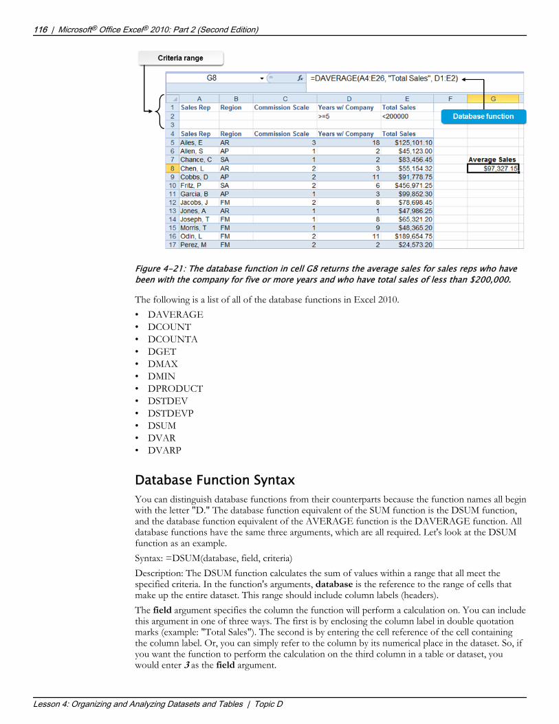
Figure 4-21: The database function in cell G8 returns the average sales for sales reps who havebeen with the company for five or more years and who have total sales of less than $200,000.

The following is a list of all of the database functions in Excel 2010.• DAVERAGE• DCOUNT• DCOUNTA• DGET• DMAX• DMIN• DPRODUCT• DSTDEV• DSTDEVP• DSUM• DVAR• DVARP

Database Function SyntaxYou can distinguish database functions from their counterparts because the function names all beginwith the letter "D." The database function equivalent of the SUM function is the DSUM function,and the database function equivalent of the AVERAGE function is the DAVERAGE function. Alldatabase functions have the same three arguments, which are all required. Let's look at the DSUMfunction as an example.Syntax: =DSUM(database, field, criteria)Description: The DSUM function calculates the sum of values within a range that all meet thespecified criteria. In the function's arguments, database is the reference to the range of cells thatmake up the entire dataset. This range should include column labels (headers).The field argument specifies the column the function will perform a calculation on. You can includethis argument in one of three ways. The first is by enclosing the column label in double quotationmarks (example: "Total Sales"). The second is by entering the cell reference of the cell containingthe column label. Or, you can simply refer to the column by its numerical place in the dataset. So, ifyou want the function to perform the calculation on the third column in a table or dataset, youwould enter 3 as the field argument.



Do Not D

uplicate

or Dist

ribute

The criteria argument specifies the criteria range. You enter this argument as a range of cells; therange must include the duplicate header row and all criteria you wish to include. It does not have toinclude the empty row between the criteria range and the dataset.Let's take another look at the previous example, which uses the DAVERAGE function.

As you can enter the field argument in three different ways, this function could be entered in any ofthe following ways.=DAVERAGE(A4:A26, "Total Sales", D1:E2)=DAVERAGE(A4:A26, E4, D1:E2)=DAVERAGE(A4:A26, 5, D1:E2)In the first example, the field argument is specified by the column's label. The second example usesthe label's cell reference. The third example specifies the argument by the column's position in thedataset. As the Total Sales column is the fifth column in the dataset, you can simply enter 5 todefine the field argument.

Note: For more information on data calculation in tables, watch the LearnTO Use StructuredReferences to Calculate Data in an Excel Table presentation from the LearnTO tile on theLogicalCHOICE Course screen.

Access the Checklist tile on your LogicalCHOICE course screen for referenceinformation and job aids on How to Use Database Functions.



You may want to showLearnTO Use StructuredReferences to CalculateData in an Excel Tablefrom the LogicalCHOICECourse screen or havestudents navigate out tothe Course screen andwatch it themselves as asupplement to yourinstruction. If not, pleaseremind students to visitthe LearnTOs for thiscourse on theirLogicalCHOICE Coursescreen after class forsupplementalinformation andadditional resources.

Do Not D

uplicate

or Dist

ribute

ACTIVITY 4-6Using Database Functions

Before You BeginThe my_author_data_04.xlsx workbook file is open, and the Authors worksheet is selected.

ScenarioAs suspected, you are being asked more and more often for summary data about Fuller andAckerman (F&A) authors based on a wide variety of criteria. Although you've been able to usesorting, filtering, and summary functions to find the answers company leaders are seeking, you feel itwould be much faster to simply type the criteria in a criteria range and use database functions toreturn the desired answers.You decide to create an answer cell to the right of the table on the Authors worksheet and use thatto query your data whenever senior leaders ask for specific information. Currently, they are lookingfor answers to the following questions:• What is the average number of books sold for authors who signed their initial contract before

2010 and who have generated more than $1 million in income?• What is the total income earned by books that were written by authors who have been with F&A

for fewer than three years or who have authored five or fewer books?

1. Create an answer cell to the right of the table to return results of database functions.a) Change the magnification level of the worksheet to 90%.b) Select cell M5 and type Answerc) Press Ctrl+Enter.d) Select Home→Styles→Cell Styles→Accent3 to apply the Accent 3 cell style to the Answer label.

2. Write a database function to answer the question "What is the average number of books sold forauthors who signed their initial contract before 2010 and who have generated more than $1 million inincome?"a) Delete the filter criteria from cells C2 and E2.b) Select cell B2, type <1/1/2010 and press Tab.c) Select cell G2, type >1000000 and press Enter.d) Select cell N5, type =DAVERAGE(A4:K816, E4, B1:G2) and press Enter.

3. What is the average number of books sold for these authors?A: 427,179

4. Write a database function to answer the question "What is the total income earned by books that werewritten by authors who have been with F&A for fewer than three years or who have authored five orfewer books?"a) Delete the contents of cells B2, G2, and N5.b) Select cell C2, type <3 and press Enter.c) Select cell E3, type <=5 and press Enter.



Do Not D

uplicate

or Dist

ribute

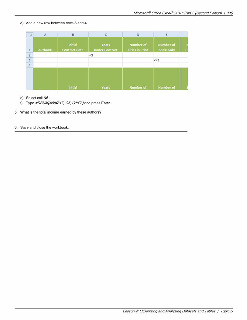
d) Add a new row between rows 3 and 4.

e) Select cell N6.f) Type =DSUM(A5:K817, G5, C1:E3) and press Enter.

5. What is the total income earned by these authors?A: $550,441,558




Do Not D

uplicate

or Dist

ribute

SummaryIn this lesson, you organized and analyzed datasets and tables. With the massive volume of datamany organizations are storing these days, the ability to organize and filter that data is a criticalelement of making sense of it all. The ability to pare down your data into manageable chunks and toask very specific questions about subsets of massive worksheets allows you to home in on what'sreally important to organizational leaders. Taking advantage of these data analysis features meansyou can get the answers you need quickly, avoid errors, and move on to other important tasks.

What advantages do you see tables providing over data ranges?

A: Answers may vary, but students are likely to find the built-in sorting, filtering, and summary functioncapabilities of tables easier to use than the alternative options for data ranges. Also, the fact thattables behave as independent objects adds a level of data integrity that data ranges don't necessarilyshare.

Which of the data-analysis tools covered in this lesson do you think will have the greatest impact on yourdaily tasks?

A: Answers will vary, largely depending on the student's role within his or her organization. Users whooften find themselves performing highly precise data analysis that digs into the minute details of largedatasets, such as business or financial analysts, will likely use advanced filtering or databasefunctions fairly often. However, users who are more interested in high-level information andcomparing overall departmental or regional performance, such as sales managers or departmentheads, may use simple sorting and filtering and subtotal functions more than other functionality.



Lesson 4: Organizing and Analyzing Datasets and Tables |


Do Not D

uplicate

or Dist

ribute

Visualizing Data withBasic ChartsLesson Time: 30 minutes

Lesson ObjectivesIn this lesson, you will visualize data with basic charts. You will:

• Create charts.

• Modify and format charts.

Lesson IntroductionExcel 2010 provides you with a powerful array of functionality for organizing and analyzingyour data. As you become more familiar with these features, you'll find you can ask Excel anastonishingly vast array of questions and get the answers you need. But not everyone whoyou report to or present data to will have the same comfort level or expertise when it comesto viewing worksheets. Viewing information in the form of ranges of data entries is simplynot natural for many people. You may find yourself presenting information to largeaudiences on a regular basis. In these cases, you don't want people scanning lines of data ona worksheet when you're trying to present. You want to give them a simple, easy-to-digestview of important data so they can quickly understand what's really important.In short, you need a way to generate visual representations of your data. Excel 2010 includessome handy functionality that can convert your raw or analyzed data into visually clear, easy-to-interpret diagrams with just a few steps. Taking the time to understand how thisfunctionality works will give you the ability to generate high-impact visuals to present tonearly any audience, nearly any time, almost instantly.

5

Do Not D

uplicate

or Dist

ribute

TOPIC ACreate ChartsLet's face it, long strings of data are simply difficult for people to read and interpret. And, in today'sdata-driven, high-pace world, most people don't have the time to sit down and pore over worksheetsto get the information they need. Often, decision makers are looking for only a snapshot of just themost relevant information. And, as an Excel user, it's likely your job to provide that snapshot forthem.Now that you've amassed, organized, and analyzed your data, you need to convert all of the figuresand labels into a picture that makes a clear, simple statement. The good news is that, in Excel, this isquite simple to do. And, what's even better, is once you convert your data in to easy-to-view visuals,you can keep those visuals up to date just as easily as you can your data.

ChartsCharts are graphical representations of the numeric values and relationships in a dataset. Charts helpworksheet viewers to quickly and easily interpret the data in a worksheet.

Figure 5-1: A pie chart on an Excel worksheet.

In this figure, while you can tell from the values in the Total Sales (in billions) column what thesales are for each market, the pie chart to the right of the data is much easier to interpret. With just aglance, you can tell that North American sales account for more sales than the other three regions,and that they account for more than a third of all sales. Getting this information from the raw datawould require a bit of analysis and some calculating.

Chart BasicsAlthough there is a wide variety of charts available in Excel 2010 to chart a number of differenttypes of data, most of the chart types follow the same basic conventions. Most of the commonlyused chart types in Excel plot data along two axes, the X axis and the Y axis. The X axis is the onethat runs horizontally along the chart. It is typically used to represent a category of information,such as fiscal quarter or department. The Y, or vertical, axis is typically used to represent valueswithin your dataset, such as sales totals or number of products shipped. The objects displayed in thechart, such as bars, columns, or lines, typically represent the individual items, or series, for whichyou wish to represent the data, such as particular regions or individual sales reps.


Lesson 5: Visualizing Data with Basic Charts | Topic A

Charts

Chart BasicsDo Not D

uplicate

or Dist

ribute

Because Excel pulls data from your worksheets to create charts, it's important to understand howExcel reads your data in order to create them. Excel pulls the elements plotted along the X axis, orthe categories, from your column labels. It identifies a data series based on the row labels from theselected dataset. Excel reads the values in the remaining cells as the values to plot against the Y axis.

Figure 5-2: Using simple sales data to chart relative sales by region.

Note that, in the figure, the categories along the X axis correspond to the worksheet column labels,which in this case are fiscal quarters. The data series, represented by the columns on the chart,represent different global regions, which Excel pulled from the row labels. The data entered into theremaining cells are the values against which the series are plotted.Of course, not all charts work exactly like this, but most of the commonly used charts do. The mostnotable exceptions are the pie chart, which you will typically use only to chart a single column ofdata, and the bar chart, which essentially turns a column chart on its side.

Chart TypesExcel 2010 includes 11 different chart types, each of which is ideal for displaying a particular type ofdata or set of relationships. Each type of chart contains a variety of specific sub-types that you canuse to tailor the presentation of your data. You can access the chart types and sub-types in theInsert Chart dialog box, which you can use to insert charts in your worksheets. You can access theInsert Chart dialog box by selecting the Insert→Charts dialog box launcher, or by selecting AllChart Types from any of the chart type drop-down menus in the Charts group on the Insert tab.



Chart Types

Do Not D

uplicate

or Dist

ribute

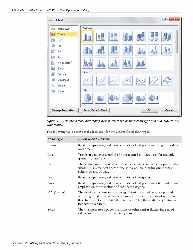
Figure 5-3: Use the Insert Chart dialog box to select the desired chart type and sub-type to suityour needs.

The following table describes the ideal uses for the various Excel chart types.

Chart Type Is Best Used to Display

Column Relationships among values in a number of categories or changes in valuesover time.

Line Trends in data over a period of time at consistent intervals, for examplequarterly or annually.

Pie The relative size of values compared to the whole and to other parts of thewhole. This is the best chart to use when you are charting only a singlecolumn or row of data.

Bar Relationships among values in a number of categories.

Area Relationships among values in a number of categories over time with visualemphasis on the magnitude of each data category.

X Y (Scatter) The relationship between two categories of measured data, as opposed toone category of measured data across evenly spaced periods of time. Usethis chart type to determine if there is a trend in the relationship betweentwo sets of variables.

Stock The change in stock prices over time or other similar fluctuating sets ofvalues, such as daily or annual temperatures.



Do Not D

uplicate

or Dist

ribute

Chart Type Is Best Used to DisplaySurface Three-dimensional representations of data. Typically, you would use a

surface chart when working with three sets of data. An example of thiswould be charting the relative change in density of several materials, at avariety of temperatures, over a period of time.

Doughnut The relative size of values compared to the whole and to other parts of thewhole. The doughnut chart type is similar to the pie chart type except youcan use this to compare relative values for more than one data series.

Bubble The relationships among three categories of measured data. The bubblechart type is similar to the X Y (Scatter) chart type. The difference is that ina bubble chart, each data point on the chart also has a relative sizecompared to the other data points. Bubble charts are often used to displaydemographic data.

Radar The aggregate relational sizes of multiple data categories in terms of multiplecriteria. For example, you could use a radar chart to track the popularity of aparticular item in multiple countries for each year in a decade.

Chart Insertion MethodsBefore inserting a chart into a worksheet, you should select the dataset the chart will be based on. Ifyou select a single cell within the desired dataset, Excel will try to guess at the proper range. Thisdoes not always generate the desired outcome, so it's a best practice to manually select the desireddataset.It's important to remember to include row and column labels in your selection and to have your dataentered correctly. For example, the categories you want plotted along the X axis should be yourcolumn labels, and the desired data series should be the row labels. Once you have ensured that yourdata is properly entered on the worksheet, and you have selected the desired range, you have threegeneral options for inserting a chart: ribbon commands, the Insert Chart dialog box, or insertingthe default chart type. For either of the first two methods, simply select the desired chart type fromthe Insert Chart dialog box or from the chart type drop-down menus in the Charts group on theInsert tab.If you know you will be inserting a number of the same type of chart in your workbook, you can setthat chart type as the default chart type. Then you can use one of two keyboard shortcuts toinstantly create the default chart type out of any selected dataset.

Note: Use the Set as Default Chart command on the Insert Chart dialog box to set thedefault chart type. This is an application-level setting, so what you set here will be the defaultchart type for any workbook file until you change the default chart type.

Keyboard Shortcut Inserts

Alt+F1 The default chart type on the same worksheet the dataset is on.

F11 The default chart type on a new worksheet.

Access the Checklist tile on your LogicalCHOICE course screen for referenceinformation and job aids on How to Create Charts.



Do Not D

uplicate

or Dist

ribute

ACTIVITY 5-1Creating a Chart

Data FileC:\091019Data\Visualizing Data with Basic Charts\sales_dashboard.xlsx


ScenarioIn addition to tracking total income by author, you also track the sales for each title by calendar year.In preparation for a big meeting with Fuller and Ackerman (F&A) leadership, you are developing asales dashboard workbook. Your goal is to create a workbook you can use to answer nearly anyquestion company leaders may have about F&A book sales. You have already organized some of theraw sales data into tables, and you have created a few charts to display overall sales information bymarket, format, and genre. Now you want to create a chart that illustrates total sales by format perfiscal year. You plan to add the chart and then position it next to the others.

1. Open the sales_dashboard.xlsx workbook file and ensure that the Sales Dashboard worksheet isselected.

Note: You may find it helpful to zoom out a bit on screen while performing thisactivity.

2. Create a line chart to display per-year sales information for the electronic and print formats.a) Scroll to the right and then select the range Y2:Z15.b) Select Insert→Charts→Line and, in the 2-D Line section, select the Line chart type.



Consider showing thestudents the raw salesdata on the Salesworksheet. This couldhelp illustrate the pointthat, although there is alot of data on theworksheet, it is not in ahighly useful state. Thisis why they are creatinga chart to help visualizethe data.

Do Not D

uplicate

or Dist

ribute

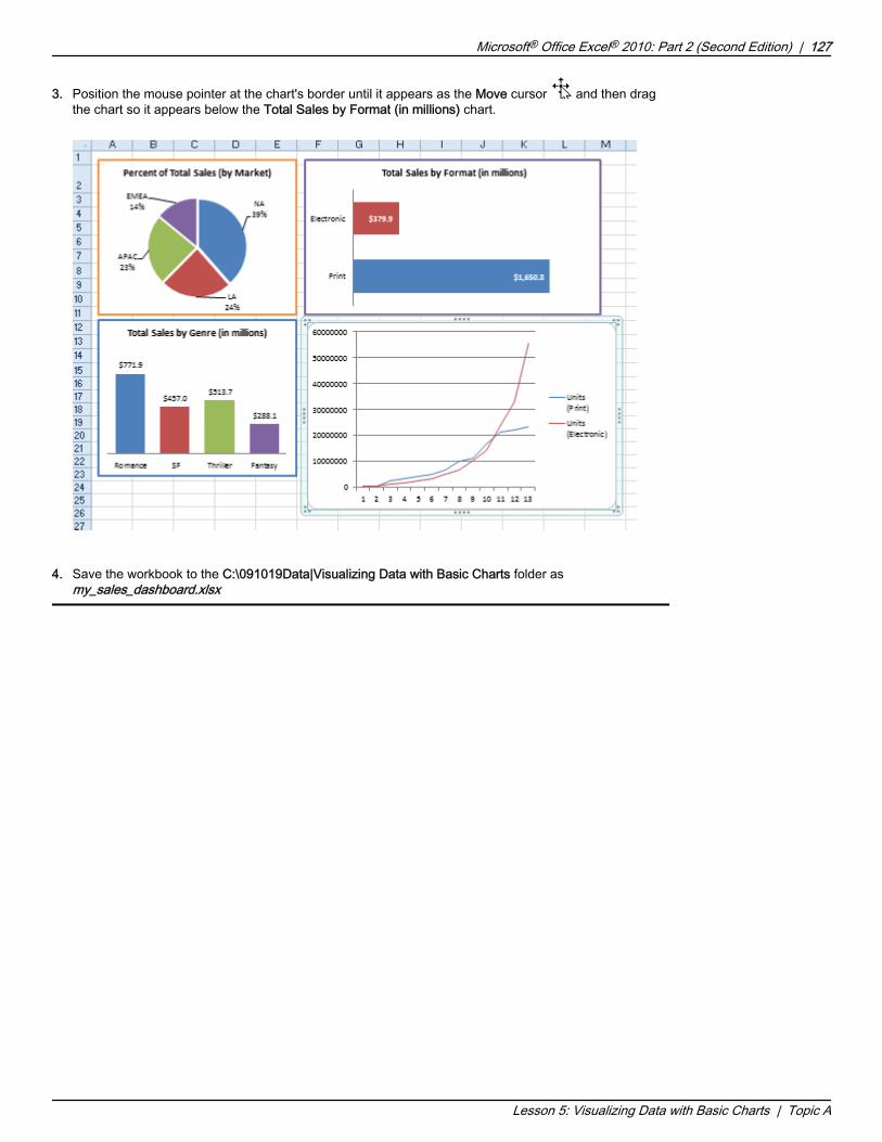
3. Position the mouse pointer at the chart's border until it appears as the Move cursor and then dragthe chart so it appears below the Total Sales by Format (in millions) chart.

4. Save the workbook to the C:\091019Data|Visualizing Data with Basic Charts folder asmy_sales_dashboard.xlsx



Do Not D

uplicate

or Dist

ribute

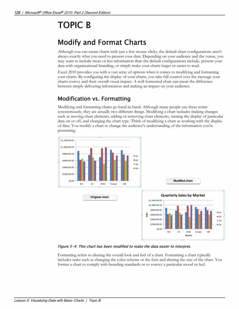
TOPIC BModify and Format ChartsAlthough you can create charts with just a few mouse clicks, the default chart configurations aren'talways exactly what you need to present your data. Depending on your audience and the venue, youmay want to include more or less information than the default configurations include, present yourdata with organizational branding, or simply make your charts larger or easier to read.Excel 2010 provides you with a vast array of options when it comes to modifying and formattingyour charts. By configuring the display of your charts, you take full control over the message yourcharts convey and their overall visual impact. A well-formatted chart can mean the differencebetween simply delivering information and making an impact on your audience.

Modification vs. FormattingModifying and formatting charts go hand-in-hand. Although many people use these termssynonymously, they are actually two different things. Modifying a chart includes making changessuch as moving chart elements, adding or removing chart elements, turning the display of particulardata on or off, and changing the chart type. Think of modifying a chart as working with the displayof data. You modify a chart to change the audience's understanding of the information you'representing.

Figure 5-4: This chart has been modified to make the data easier to interpret.

Formatting refers to altering the overall look and feel of a chart. Formatting a chart typicallyincludes tasks such as changing the color scheme or the font and altering the size of the chart. Youformat a chart to comply with branding standards or to convey a particular mood or feel.


Lesson 5: Visualizing Data with Basic Charts | Topic B

Modification

FormattingDo Not D

uplicate

or Dist

ribute

Figure 5-5: This chart has been formatted to comply with branding guidelines.

Chart ElementsChart elements are the individual objects that can appear on charts and that convey some level ofinformation to a viewer about the chart's data. While all Excel charts contain at least one chartelement, by default, the various chart types display different chart elements. For example, while barand column charts typically display an X and a Y axis, surface charts display three axes. Pie anddoughnut charts don't contain axes as they deal with only a single column of data. Each chartelement serves a different role in visually communicating information about data and trends.

Figure 5-6: Chart elements help the audience interpret chart data.



Chart Elements

Do Not D

uplicate

or Dist

ribute

Guidelines for Including Chart ElementsNote: All of the Guidelines for this lesson are available as checklists from the Checklist tile onthe LogicalCHOICE Course screen.

Formatting charts has relatively little impact on an audience's ability to interpret your data.Modifying chart elements, on the other hand, can have a significant impact. As a general rule, it'sbest to include only those chart elements that are absolutely necessary for conveying meaning.Cluttered charts can muddy your main point and make the chart confusing to view, which is exactlywhat you create charts to avoid. However, some chart elements do actually help add meaning. Untilyou gain an intuitive sense of what chart elements to include for various purposes, you may want toconsider adding chart elements that you feel will help your target audience interpret your data,analyze your chart, and then remove anything that doesn't directly contribute to the message youintend to deliver. When analyzing your charts, ask yourself questions, such as:• If I remove the gridlines, will the chart still convey meaning?• Do I need a legend? Can I remove the legend and use data labels instead?• How much precision do I need for axis labels?• Do the axes really need titles?• Will using a three-dimensional layout enhance visual appeal or distort proportions?• Does including the data table aid understanding?• Do I really need major and minor tick marks on the axes?• Before finalizing your charts, keep the old adage "less is more" in mind. If the audience needs an

element to acquire meaning, keep it. Otherwise, remove it.

The Chart Tools Contextual TabYou can access all of the commands you will use to modify and format your charts on the ChartTools contextual tab. Similar to other contextual tabs, the Chart Tools contextual tab appearswhenever you select a chart or a chart element, and it disappears when you select a worksheetelement outside the chart. The Chart Tools contextual tab contains three tabs that each containtask-related groups and commands for working with your charts. Let's take a look at the variouscommand groups on each of these tabs.

Figure 5-7: The Design tab.

Use the commands on the Design tab to quickly change the overall look and feel of your charts.

Design Tab CommandGroup

Contains Commands For

Type Changing the chart type and saving a particular chart as a template.

Data Changing the chart's dataset range and switching the row and columndata. Keep in mind that this does not switch the data that is displayedon the X axis with the data that is displayed on the Y axis. Thisswitches the categories with the data series.

Chart Layouts Quickly configuring the display of chart elements according topredefined configurations.

Chart Styles Quickly formatting a chart by using predefined sets of formattingoptions.



The Design Tab

Do Not D

uplicate

or Dist

ribute

Design Tab CommandGroup


Location Moving charts to different worksheets within a workbook.

Figure 5-8: The Layout tab.

Use the commands on the Layout tab to work with individual chart elements and to name charts.

Layout Tab CommandGroup


Current Selection Selecting particular chart elements and accessing the FormatSelection dialog box.

Insert Adding images, shapes, and text boxes to your charts.

Labels Toggling on or off and configuring the display of chart elements.

Axes Toggling on or off and configuring the display of axes and gridlines.

Background Configuring the display of chart background elements.

Analysis Adding and configuring data analysis chart elements.

Properties Naming charts.

Figure 5-9: The Format tab.

Use the commands on the Format tab to configure chart formatting.

Format Tab CommandGroup


Current Selection Selecting particular chart elements and accessing the FormatSelection dialog box.

Shape Styles Configuring formatting options for chart elements.

WordArt Styles Configuring formatting options for chart text.

Arrange Changing the front-to-back placement of chart elements andconfiguring the orientation of chart elements.

Size Changing the size of chart elements.

The Select Data Source Dialog BoxYou will use the Select Data Source dialog box to manage Excel chart data. From here, you canedit the entire dataset feeding the chart, or you can edit the data feeding any of the individual dataseries. You can also remove from or add back to the chart any of the individual data series, reorder



The Layout Tab

The Format Tab

The Select Data SourceDialog Box

Do Not D

uplicate

or Dist

ribute

how the data series appear on the chart, or switch the chart's X and Y axes. You can access theSelect Data Source dialog box from the Chart Tools contextual tab by selectingDesign→Data→Select Data.

Figure 5-10: Use the Select Data Source dialog box to manage the data displayed by Excel charts.

Access the Checklist tile on your LogicalCHOICE course screen for referenceinformation and job aids on How to Modify and Format Charts.



Do Not D

uplicate

or Dist

ribute

ACTIVITY 5-2Modifying and Formatting a Chart

Before You BeginThe my_sales_dashboard.xlsx workbook file is open and the Sales_Dashboard worksheet isselected.

ScenarioYour new line chart is in place alongside the other charts in your sales dashboard workbook. Itdoesn't blend visually with the other charts on the worksheet, so you decide to format it to matchthe others. You also feel the Total Sales by Format (in millions) chart doesn't quite visuallyconvey the message you want to send, which is how much of overall sales are made up of eachformat. You decide to convert that bar chart into a pie chart.

1. Add a title to the line chart.a) Ensure the line chart is selected and, on the Chart Tools contextual tab, select the Layout tab.b) In the Labels group, select Chart Title→Centered Overlay Title.c) In the Formula Bar, type Unit Sales by FY (in millions) and press Enter.d) With the chart title still selected, right-click the title and, by using the mini toolbar, change the font

size to 12

2. Edit the chart legend to make it easier to read.a) From the Chart Tools contextual tab, select Design→Data→Select Data.b) In the Select Data Source dialog box, in the Legend Entries (Series) section, select Units(Print) and

then select Edit.c) In the Edit Series dialog box, delete the contents of the Series name field, type Print and select OK.

Note: When you edit legend entries in this way, as opposed to changing thelabels in the source dataset, Excel breaks the link between the label in thedataset and the legend entry. If you modify the label in the original dataset, thenew text will not update in the legend.

d) Use the same method to change Units(Electronic) to Electronice) In the Select Data Source dialog box, select OK.f) Verify that the changes reflect in the chart legend.

3. Remove the chart's gridlines.a) Ensure that the chart is still selected and, on the Chart Tools contextual tab, select the Layout tab.



Do Not D

uplicate

or Dist

ribute

b) In the Current Selection group, select the Chart Elements down arrow above the Format Selectioncommand.

Note: The selection in the Chart Elements drop-down menu may be differentin this image if you inadvertently selected a chart element manually.

c) From the Chart Elements drop-down menu, select Vertical (Value) Axis Major Gridlines and pressDelete.

4. Edit the horizontal axis.a) Select the down arrow in the Current Selection group and select Horizontal (Category) Axis.b) From the Chart Tools contextual tab, select Design→Data→Select Data.c) In the Select Data Source dialog box, in the Horizontal (Category) Axis Labels section, select Edit.d) In the Axis Labels dialog box, in the Axis label range field, select the Collapse Dialog button.e) Select the range X3:X15 and press Enter.f) In the Axis Labels dialog box, select OK and, in the Select Data Source dialog box, select OK.g) Verify that the horizontal axis is now labeled with the calendar years.

Note: The original chart didn't contain the year labels because the originaldata selection did not contain the year labels. This is due to the table layoutand the chart type used here.

5. Edit the vertical axis.a) Ensure that the chart is still selected.b) From the Chart Tools contextual tab, select the Layout→Current Selection down arrow and then

select Vertical (Value) Axis.c) Select Layout→Current Selection→Format Selection.d) In the Format Axis dialog box, select the Number tab.e) In the Category section, select Custom.f) Clear the contents of the Format Code field and type ##0,,

g) Select Add.



Let students know thatit's not necessary tounderstand theparticulars of numberformatting code here. Itis more important tounderstand that they canapply the same types ofnumber formatting tochart elements as theycan to cell entries.

Do Not D

uplicate

or Dist

ribute

h) In the Format Axis dialog box, select Close.

6. Resize the chart.a) Select the chart border to ensure that the entire chart, and not the vertical axis, is selected; then

select the Format tab on the Chart Tools contextual tab.b) In the Size group, set the value in the Height spin box to 2.5.c) Set the value in the Width spin box to 4.8.

7. Edit the chart to make it more easily read.a) Right-click the legend and select Format Legend.b) In the Format Legend dialog box, make sure the Legend Options tab is selected.c) In the Legend Position section, select the Top radio button and then select Close.d) Drag the legend so it is centered directly below the chart title.

e) Right-click the horizontal axis and select Format Axis.f) In the Format Axis dialog box, make sure the Axis Options tab is selected.g) At the bottom of the Axis Options pane, in the Position Axis section, select the On tick marks radio

button and select Close.

8. Add a border to the chart.a) With the chart still selected, if necessary, select Chart Area from the Chart Elements drop-down

menu.b) In the Current Selection group, select Format Selection.c) In the Format Chart Area dialog box, select the Border Color tab.d) Ensure that the Solid line radio button is selected and select the Color down arrow.e) From the Color gallery, in the Standard Colors section, select Light Green.f) Select the Border Styles tab.g) Set the value in the Width spin box to 2 and select Close.

9. Deselect the chart to view the border.




Do Not D

uplicate

or Dist

ribute

SummaryIn this lesson, you gave your worksheet data visual interest by using basic charts. You did this bycreating charts to display your data and formatting and modifying them to make them easier to readand interpret. Providing your audience members with a visual snapshot of your data enables them toquickly see the overall impact raw data, recognize trends, make easy comparisons, and focus on yourmessage instead of your worksheets.

What are a couple of reasons you anticipate for including charts in your workbooks?

A: Answers will vary, but many users will likely find charts useful for regular meetings at which statusupdates are frequently presented. The use of charts is a quick and easy way to demonstrateprogress. Also, users are likely to find charts helpful when breaking down overall and periodic figures,such as at end-of-year events or when reviewing the success of a particular initiative or product.

Which chart type do you expect to use most often?

A: Answers will vary as a direct function of a person's job role. Typically, people will use pie charts todisplay visual information on a single series of data or column charts to examine the relationshipsamong a set of values.



Lesson 5: Visualizing Data with Basic Charts |


Do Not D

uplicate

or Dist

ribute

Analyzing Data withPivotTables, Slicers, andPivotChartsLesson Time: 1 hour

Lesson ObjectivesIn this lesson, you will analyze data with PivotTables, Slicers, and PivotCharts. You will:

• Create a PivotTable.

• Analyze PivotTable data.

• Present data with PivotCharts.

• Filter data by using slicers.

Lesson IntroductionYou've already seen the way Excel functions and features, such as sorting, filtering, andsummary functions, can help you drill down into your data to get answers to very specificquestions. Although using these features is often a good option for attaining specificanswers, these aren't necessarily the best options if you need to frequently change thequestions you're asking of your data. To change the question you're asking when usingfunctions, sorting, and filtering, you often need to rewrite functions, adjust criteria, or re-filter you data; sometimes, you need to use several of these methods at the same time. Youcertainly could take this route, but it isn't the most efficient way to re-query your data to getthe variety of answers you need. If you work in a high-paced, data-intensive environment,you simply may not have the time needed to recalculate every time a supervisor asks you adifferent question. You need something a little more dynamic.Excel 2010 includes a powerful feature that enables you to ask any number of questions ofyour data; get detailed, specific answers; and do it all over again in just a matter of moments.By using PivotTables to analyze your data, you will take the next major step toward Excelmastery. This functionality gives you a staggering level of control over data analysis. Youcan get critical, time-sensitive organizational intelligence to the people who need it quickly,easily, and with a high-level of flexibility.

6

Do Not D

uplicate

or Dist

ribute

TOPIC ACreate a PivotTableTo take advantage of the functionality and flexibility of PivotTables, you must first understand howto create them. Although this is a relatively simple process, you must also know a bit about the typeof data that works best for PivotTables. By taking a few moments to gain this foundational level ofunderstanding, you'll be preparing yourself to create useful, effective PivotTables that you can use toanalyze your raw data in incredibly fine detail.

PivotingPivoting allows you to view your data from a variety of new perspectives. In Excel, pivoting is a formof data manipulation that can take a column of data and pivot it into a row and vice versa. While thismay not seem highly useful at first, think about it in terms of reorganizing and summarizing databased on a number of criteria. For example, let's say you have a dataset that contains rows of data,each representing a single event, such as a sale, a shipment, or a financial transaction. Each rowwould be composed of cells in a series of columns that each represent a single aspect of theindividual events, say a particular date, dollar amount, or location. If you want to compile particulardata about these events as a whole, say to find total sales that occurred at each of the variouslocations, you could take the location column and pivot it so that it appears as a series of rows witheach unique location being represented by an individual row. Location is your first criterion.Your second criterion is sales figures. In the original dataset, each row represents a single sale. Thesales figures for all of the sales were in the same column, and each was associated with one of thelocations. Now that the locations are represented by individual rows in the pivoted dataset, you wantto know the total value of all sales from the dataset for each location. Manually calculating thiswould take some time; however, asking Excel to look at every sales entry for each location, sum thevalues together, and then return the total value for each location in the new rows would save all thatmanual effort. Once done, you would have just successfully pivoted a single column into multiplerows and summarized a particular data entry for each to answer a very specific question: How muchin total sales was generated for each location? This simple example shows the power of pivoting.

Note: As with filtering and sorting, pivoting does not affect your raw data; it only modifies yourview of the data.

Here's a look at how the previous example would work in a worksheet.


Lesson 6: Analyzing Data with PivotTables, Slicers, and PivotCharts | Topic A

Pivoting

Do Not D

uplicate

or Dist

ribute

Here, you can see that, in the original dataset, each sale is listed as a separate entry. Store locations,in the form of location codes, appear within a single column. In the pivoted dataset, that column hasbeen pivoted into rows, with each location being represented by a single row. For each location,Excel has summed each sale and calculated the total sales per store. Excel also calculated the total ofall sales for all locations.

PivotTablesA PivotTable is a dynamic Excel data object that enables you to analyze data by pivoting columns androws of raw data without altering the raw data. PivotTables are effective for summarizing largevolumes of data according to two or more criteria to return specific answers to your questions.PivotTables combine some of the most powerful and useful types of Excel functionality, such assorting, filtering, summary functions, and subtotals, to give you an incredible level of control overhow you view your data.When you create a PivotTable, Excel enables you place it on the same worksheet as the originaldata, or you can insert it on a new worksheet. Once the PivotTable is created, you can re-pivot, re-sort, re-summarize, and re-filter you data any number of times without affecting the original dataset.In addition to pivoting columns and rows, you can nest columns and rows within one another tocreate a hierarchy, much as you do when using subtotals. You can expand or collapse levels ofhierarchy to view more or less detail in your PivotTables. And you can use any of the availablesummary functions to summarize your pivoted data for a variety of purposes. You can also createPivotTables out of either data in the same workbook or data from other workbooks and externaldata sources.



PivotTables

Do Not D

uplicate

or Dist

ribute

Figure 6-1: A PivotTable containing a hierarchy of raw data. In this example, genre, market, sellprice, and total earnings to date are all column labels in the original dataset.

Transactional DataThere is an extremely important consideration for you to keep in mind when creating and workingwith PivotTables: your data format. PivotTables are designed to work with, and work best with, rawtransactional data. Transactional data is not summarized in any way, so it does not contain row labels,only column labels. Columns in a transactional dataset are also known as fields. The best way tovisualize transactional data is to examine the root word "transaction." In a transactional dataset, eachtransaction, or entry, is located in its own separate row. To carry on the example from earlier, of salestransactions at a variety of locations, each sale, regardless of when or where it took place, would beentered as an individual row of data. The dataset columns represent the specific elements of eachtransaction: date, time, location, amount, and so on.In a summarized dataset, even a raw one, the data has already been compiled in some way and willhave row labels as well as column labels. For example, you may have raw sales data for each salesrep in your organization. Because each rep has his or her own row of data, the dataset would likelycontain the total of each person's sales, as opposed to each sale regardless of the rep. Although youcan create PivotTables from summary data, they will never give you as much granular insight intoyour data as PivotTables created from transactional data.



Transactional Data

Do Not D

uplicate

or Dist

ribute

Figure 6-2: Transactional data shows each event, whereas summary data compiles it in someway.

The Create PivotTable Dialog BoxYou use the Create PivotTable dialog box to insert PivotTables into your worksheets. From here,you can select the desired dataset or include a reference to a named range or table. You can alsoselect a location for the PivotTable, which can be on the same worksheet as the dataset or onanother worksheet in the same workbook. You can access the Create PivotTable dialog box byselecting Insert→Tables→PivotTable.

Figure 6-3: The Create PivotTable dialog box.

Access the Checklist tile on your LogicalCHOICE course screen for referenceinformation and job aids on How to Create a PivotTable.



The Create PivotTableDialog Box

Do Not D

uplicate

or Dist

ribute

ACTIVITY 6-1Creating a PivotTable

Data FileC:\091019Data\Analyzing Data with PivotTables, Slicers, and PivotCharts\sales_dashboard_06.xlsx


ScenarioYour supervisor and other senior managers at Fuller and Ackerman continue to come to you foranswers to questions they have about authors and book sales. Given the frequency with which youfind yourself analyzing data, you decide it would be most efficient to add a PivotTable to your salesdashboard workbook. With such a PivotTable, you'll be able to answer any number of questionswithout having to significantly revise your worksheets. You have already defined a name for the rawsales data on the Sales worksheet in the sales dashboard workbook, so you will create the PivotTableby using that defined name.

1. Open the sales_dashboard_06.xlsx workbook file.

Note: You may find it helpful to zoom out slightly during this activity.

2. Insert a PivotTable by using a defined name.a) Scroll to the right and select cell AD2.b) Select Insert→Tables→PivotTable.c) In the Create PivotTable dialog box, in the Choose the data that you want to analyze section, ensure

that the Select a table or range radio button is selected.d) In the Table/Range field, type RawSalesDatae) In the Choose where you want the PivotTable report to be placed section, make sure the Existing

Worksheet radio button is selected.



As an alternative to step2b, remind the studentsthey can use the InsertPivotTable commandthey added to both theQAT and the ribbon inLesson 1.RawSalesData is thedefined name for theentire raw sales dataseton the Sales worksheet.

Do Not D

uplicate

or Dist

ribute

f) In the Location field, verify that 'Sales Dashboard'!$AD$2 is displayed.

g) Select OK.

3. If necessary, scroll to the right so the PivotTable is fully visible and not obstructed by the PivotTableField List pane.

4. In the PivotTable Field List pane, verify that the Choose fields to add to report list displays a list of all ofthe fields in the dataset on the Sales worksheet.

5. Save the workbook to the C:\091019Data\Analyzing Data with PivotTables, Slicers, and PivotChartsfolder as my_sales_dashboard_06.xlsx



Let the students knowyou will be covering thePivotTable Field Listpane in the next topic.For now, it's justimportant for them torealize that Excelcreated the PivotTableby using all of the fieldsin the dataset.

Do Not D

uplicate

or Dist

ribute

TOPIC BAnalyze PivotTable DataNow that you have created your PivotTable, you're ready to dive right in and crunch the numbers togain the organizational insight that can help you succeed. As with all Excel data analysis tasks,creating and configuring effective PivotTables is a matter of asking the right questions to glean thenecessary information. When working with PivotTables, this all boils down to structure. You alreadyknow PivotTables allow you to reorganize and re-analyze your data as many times as necessary toget all of the answers you're looking for. How do you translate your questions into a PivotTablestructure? Actually, it's relatively simple.Excel 2010 provides you with a number of different tools and commands you can use to organizethe structure of your PivotTables. Knowing how these tools work, and understanding howPivotTable structure translates into actionable intelligence, are the keys to getting the answers youseek.

Start with Questions, End with StructureTo create PivotTables that will be useful to you, begin by thinking about the types of questions youwould like your raw data to answer. This is precisely that same type of initial analysis you performwhen determining which functions or formulas to include in worksheets. The only difference here isthat you will use your questions as a basis for organizing your PivotTables, not to enter a function ora formula. Once you've determined what question you want Excel to answer, you can begin todesign the structure of your PivotTable.There are a couple of items to keep in mind before beginning this process. First, it's typically best tocreate rows and columns out of fields that have a fairly finite set of entries, such as sales reps,regions, or products. You may not, for example, find it very useful to create rows out of dates thatoccurred over a 10-year span of time as you could end up with thousands of rows of data. Second,you should create rows out of the field for which you are primarily interested in determining somefact, and create columns out of your secondary criterion. For example, if you want to know the totalsales per product for each sales rep in your department, you would typically create rows out of salesreps (your primary concern) and columns out of the products (the items for which you aremeasuring performance). Then you would ask Excel to use the SUM function to total the sales foreach rep per product.Let's take a look at a simple example. This is the beginning of a table with about 100 entries of salesdata.


Lesson 6: Analyzing Data with PivotTables, Slicers, and PivotCharts | Topic B

While it is a general ruleof thumb to create rowsand columns from fieldswith relatively smallnumbers of uniqueentries, you can letstudents know that it issometimes necessary tocreate PivotTables thatcontain large numbers ofrows or columns.

Do Not D

uplicate

or Dist

ribute

Now, here's a PivotTable created from the entire dataset that answers this question: What are thetotal sales for each sales rep by product?

Notice that the sales reps are listed by row and the products are listed by column. The PivotTablereturns the total sales, indicating the use of the SUM function, for each sales rep for each product.Now, let's say you'd like Excel to answer the following question: How many of each product wassold in each region? As you are primarily concerned with what is happening on a per-region basis,you would make regions the rows and keep the products in columns. Then you would ask Excel tocount the number of each product sold in each region, indicating the use of the COUNT function.

Notice that the rows and columns in each of these examples represent two of the criteria on whichyou are analyzing the data. The values throughout the rest of the table represent the third criterion,



Do Not D

uplicate

or Dist

ribute

the values you are asking Excel to calculate based on the other two criteria. This is the basicstructure you will use to create most PivotTables. The keys to structuring your PivotTables are todetermine the question you want Excel to answer, to visualize the table you wish to create, and todetermine what calculation you want Excel to perform.

The PivotTable Field List PaneOnce you create a PivotTable, you will use the PivotTable Field List pane to configure thePivotTable and perform data analysis tasks. Excel automatically opens PivotTable Field List panewhen you insert a PivotTable in a worksheet. The top half of the pane, the Choose fields to add toreport section, displays a list of all of the fields (columns) from the original dataset; Excel pulls thenames for these from the column labels. The bottom half of the pane, the Drag fields betweenareas below section, displays a series of four areas that you use to configure the PivotTable. Bydragging the various fields to the various areas, you configure the structure of the PivotTable andselect the values upon which Excel performs calculations.As PivotTables are dynamic, by default, you can drag fields to the various areas of the PivotTableField List pane as necessary and your PivotTable will update automatically. You can move thefields around as often as you like, and you can include more than one field in each area. When youdrag more than one field into the same area, Excel creates a hierarchy in the PivotTable with itemson top of the area representing higher levels in the hierarchy. This works much like using subtotalsand outlines in ranges.Each field that you have dragged into an area displays a field down arrow. This provides you withaccess to context menus and dialog boxes that enable you to configure your PivotTables further.



The PivotTable Field ListPane

Do Not D

uplicate

or Dist

ribute

Figure 6-4: Use the elements of the PivotTable Field List pane to configure the structure ofPivotTables.

The following table provides a brief description of the various elements of the PivotTable FieldList pane.

PivotTable Field List PaneElement

Description

Layout menu down arrow Provides you with access to a menu that contains various pre-configured PivotTable Field List pane layouts. Select fromamong these options to customize the PivotTable Field Listpane to suit your needs.

Field check boxes These allow you to add or remove fields from the various areas.Checking a field's check box adds it to an area, whereasunchecking it removes the field from all areas. You have nocontrol over where Excel places a field when you check its checkbox, so many users prefer to simply drag the fields to the desiredareas.



Do Not D

uplicate

or Dist

ribute

PivotTable Field List PaneElement

Description

Field down arrow Selecting a field's down arrow displays a context menu thatprovides you with various options for configuring yourPivotTables. For example, you can move fields to another area(again, this can also be done simply by dragging the field toanother area), move fields within a hierarchy, or access the FieldSettings or Value Field Settings dialog boxes.

Report Filter area Drag fields here to include field values as filter criteria for thePivotTable.

Column Labels area Drag fields here to create columns out of the unique entries in afield.

Row Labels area Drag fields here to create rows out of the unique entries in a field.

Values area Drag fields here to have Excel perform calculations on, orsummarize, their values.

Note: To learn more about tailoring PivotTables to suit your specific needs, watch the LearnTOCustomize the View of a PivotTable presentation from the LearnTO tile on theLogicalCHOICE Course screen.

The PivotTable Tools Contextual TabThe PivotTable Tools contextual tab displays commands and options that are specific to workingwith PivotTables. In a similar way as other contextual tabs, the PivotTable Tools contextual tabappears when you select a PivotTable and disappears when you select outside the PivotTable. ThePivotTable Tools contextual tab contains two tabs: the Options tab and the Design tab.

Figure 6-5: The Options tab.

The following table identifies the types of commands you will find in the various groups on theOptions tab.

Options Tab Group Contains Commands For

PivotTable Accessing the PivotTable Options dialog box, which allows you tochange global PivotTable settings. This also displays the name of thecurrently selected PivotTable.

Active Field Changing the currently selected field's settings.

Group Grouping various elements within a PivotTable and managing thosegroups.

Sort & Filter Accessing and managing sorting and filtering commands and options.

Data Refreshing PivotTable data when the source dataset has been updated,and for modifying the dataset that feeds PivotTables.

Actions Clearing filtering, selecting elements of a PivotTable, and movingPivotTables in your workbooks.



You may want to showLearnTO Customize theView of a PivotTablefrom the LogicalCHOICECourse screen or havestudents navigate out tothe Course screen andwatch it themselves as asupplement to yourinstruction. If not, pleaseremind students to visitthe LearnTOs for thiscourse on theirLogicalCHOICE Coursescreen after class forsupplementalinformation andadditional resources.The Options Tab

Do Not D

uplicate

or Dist

ribute

Options Tab Group Contains Commands ForCalculations Configuring PivotTable calculations.

Tools Creating PivotCharts, performing data analysis tasks, and working with aparticular type of external database.

Show Toggling the display of PivotTable elements on and off.

Figure 6-6: The Design tab.

The following table identifies the types of commands you will find in the various Design tabgroups.

Design Tab Group Contains Commands For

Layout Toggling particular functionality on or off, and for modifying the overalllayout of PivotTables.

PivotTable StyleOptions

Toggling the display of PivotTable elements on or off.

PivotTable Styles Selecting and configuring PivotTable formatting options.

The Value Field Settings Dialog BoxWhen you select the field down arrow of a field in the Value area of the PivotTable Field Listpane, Excel opens the Value Field Settings dialog box. You will use the commands and options inthe Value Field Settings dialog box to configure the calculations Excel performs on field data inPivotTables, and to configure how Excel displays the results of those calculations. The Value FieldSettings dialog box is divided into two tabs: the Summarize Values By tab and the Show ValuesAs tab.



The Design Tab

The Value Field SettingsDialog Box

Do Not D

uplicate

or Dist

ribute

Figure 6-7: The Value Field Settings dialog box.

The Summarize Values By tab enables you to select which function Excel uses to summarize thedata in your PivotTables. The available functions here are the same as those available for creatingsubtotals and for summarizing table data. For example, you could use the SUM function to find thetotal of all values that meet the criteria outlined in the PivotTable rows and columns. Or, you coulduse the AVERAGE function to find the average values of the entries that meet the criteria.

Note: The default summary function to numerical values is the SUM function. The defaultsummary function for all other values is the COUNT function.

The Show Values As tab provides you with access to options for how you wish to display yoursummarized PivotTable data. By default, the value here is No Calculation, which means thePivotTable will simple summarize your data according to the function selected on the SummarizeValues By tab. You can also choose to have Excel display the summary data in a variety of otherways. For example, you may wish to show the summarized data as a percentage of the grand total oras a percentage of column or row totals. This could be helpful if you want to know what percentageof your total sales came from a particular region or which sales rep generated the highest percentageof your total or regional sales. Or, you may wish to show a relative comparison between values. Forexample, you may wish to see how far behind the sales leader other sales reps are in terms of totalsales.One other handy feature of the Value Field Settings dialog box is the Number Format button.Selecting this will open a scaled-down version of the Format Cells dialog box, which contains onlythe Number tab. Use this to change the cell formatting in your PivotTables to accommodate thevarious types of values you ask Excel to calculate.

Summarize and Show CombinationsCombining the options from the Summarize Values By tab and the Show Values As tab enablesyou to gain a deeper understanding of the information in your raw data. Here is a simple examplethat shows how the summary functions and the Show Values As tab options work together to giveyou new perspectives on your data. Take a look at this PivotTable that displays sales totals for salesreps per region. Here, the sales figures have been dragged to the Values area of the PivotTableField List pane, and the default SUM function and No Calculation option are selected.



SUM Function OnlyDo Not D

uplicate

or Dist

ribute

Now take a look at how selecting the % of Grand Total option from the Show Values As tabchanges your view of the data; the summary function is still the SUM function.

You can see what percentage of all sales is comprised of each rep's sales in each region. Notice alsothat the grand totals for each row and for each column add up to 100 percent of all total sales. Younow have a clear picture of which regions and which sales reps are generating your sales.Now take a look at what happens when you change the summary function to the AVERAGEfunction and change the Show Values As tab option to Difference From. Here, all sales rep's salesaverages are being compared to Robert Toner's sales, as he has the highest percentage of overallsales. You could compare the values to any individual sales rep.

Notice that there are no values for Robert Toner, as his values are the ones the PivotTable iscomparing the other values to. By looking at this PivotTable, you can see how far behind the salesleader all other reps are in terms of average regional and overall sales. You can even tell that J. Riosis actually ahead of Robert Toner in two regions, the Northeast and the Southwest. Combiningsummary functions with the show values as options is an effective way to gain a deep, granularunderstanding of the information hidden in your raw data.

Access the Checklist tile on your LogicalCHOICE course screen for referenceinformation and job aids on How to Analyze PivotTable Data.



Percentage of Total

Difference From Options

Do Not D

uplicate

or Dist

ribute

ACTIVITY 6-2Analyzing PivotTable Data

Before You BeginThe my_sales_dashboard_06.xlsx workbook file is open.

ScenarioWith your PivotTable in place, you're now ready to answer some of the questions Fuller andAckerman senior managers have been asking. Here is a list of their current requests:• What is the total number of units sold per genre in each of the markets served?• Which genre is the biggest overall seller?• For the APAC and EMEA markets, what is the combined number of total units sold in the

romance and fantasy genres?• What percentage of total sales is made up of fantasy sales in the LA market?• Which market has the highest percentage of science fiction sales?• For each author and book, what are the total sales of electronic books versus the total sales of

print books?• Which author has the lowest total sales?• For the lowest-selling author, which book has generated the most sales?• What percentage of author 1048's total sales are electronic book sales?

1. Structure the PivotTable to answer the question "What is the total number of units sold per genre ineach of the markets served?"a) Ensure the Sales Dashboard worksheet is selected, and then select any cell within the PivotTable.b) In the PivotTable Field List pane, drag the Genre field from the Choose fields to add to report list to

the Row Labels area.c) Drag the Market field to the Column Labels area.



Do Not D

uplicate

or Dist

ribute

d) Drag the Total Units to Date field to the Values area.

e) If necessary, scroll to the right so the PivotTable is visible.

2. Review the totals in the data cells to determine the total number of units sold per genre in each market.

3. Use the PivotTable to answer the question "Which genre is the biggest overall seller?"a) Select any cell in the range AI4:AI7.

b) On the PivotTable Tools contextual tab, select Options→Sort & Filter→Sort Largest to Smallest.

4. Which genre is the biggest overall seller?A: Romance with 110,272,958 copies sold

5. Use the PivotTable to answer the question "For the APAC and EMEA markets, what is the combinednumber of total units sold in the romance and fantasy genres?"



Do Not D

uplicate

or Dist

ribute

a) From the Column Labels drop-down menu on the PivotTable, uncheck the (Select All) check box,and then check both the APAC check box and the EMEA check box.

b) Select OK.c) From the Row Labels drop-down menu, uncheck the (Select All) check box and then check the

Fantasy and Romance check boxes.d) Select OK.

6. What is the total number of units of fantasy and romance books sold in the APAC and EMEA markets?A: 64,309,243

7. Use the PivotTable to answer the question "What percentage of total sales is made up of fantasy salesin the LA market?"a) Clear all filters in the Row Labels drop-down menu and in the Column Labels drop-down menu.b) In the PivotTable Field List pane, in the Values area, select the Sum of Total down arrow.

c) In the drop-down menu, select Value Field Settings.d) In the Value Field Settings dialog box, select the Show Values As tab.e) In the Show values as drop-down menu, select % of Grand Total and then select OK.

8. What percentage of total sales is made up of fantasy sales in the LA market?A: 2.91 percent

9. Use the PivotTable to answer the question "Which market has the highest percentage of science fictionsales?"



If students have issueswith the PivotTable FieldList pane closing, it maybe because the selectedcell is no longer withinthe PivotTable afterfiltering. Let them knowthey can simply selectany cell within thePivotTable to re-displaythe PivotTable Field Listpane.

Do Not D

uplicate

or Dist

ribute

a) In the PivotTable Field List pane, in the Values area, select the Sum of Total down arrow, and thenselect Value Field Settings.

b) Select the Show Values As tab and then select % of Row Total from the Show values as drop-downmenu.

c) Select OK.d) Filter the PivotTable to display only the science fiction (SF) genre.

10. Which market has the highest percentage of science fiction sales?A: The NA market with 26.84 percent.

11. Clear the filter.

12. Restructure the PivotTable to answer the question "For each author and book, what are the total salesof electronic books versus the total sales of print books?"a) Drag the Genre field, the Market field, and the Total Units to Date field back to the Choose fields to

add to report list.b) Drag the Author field to the Row Labels area.c) Drag the Title field to the Row Labels area, making sure you drop it below the Author field.

d) Drag the Format field to the Column Labels area.e) Drag the Total Earnings to Date field to the Values area.f) Right-click any data cell within the PivotTable and select Value Field Settings.g) In the Value Field Settings dialog box, select Number Format.h) In the Format Cells dialog box, in the Category list, select Currency and then select OK.i) Select OK.j) Scroll down the PivotTable to review the total sales of electronic and print books for each author and

title.

13. Use the PivotTable to answer the question "Which author has the lowest total sales?"a) Select cell AG4.b) On the PivotTable Tools contextual tab, select Options→Sort & Filter→Sort Smallest to Largest.

14. Which author has the lowest total sales?A: Author 1017 with $5,454,183.55

15. Sort the results for author 1017 to answer the question "For the lowest-selling author, which book hasgenerated the most sales?"a) Select any cell within the range AG5:AG10.b) On the PivotTable Tools contextual tab, select Options→Sort & Filter→Sort Largest to Smallest.

16. Which book for author 1017 has generated the most sales?A: BookTitle0135 with $2,390,754.44 in sales

17. Use the PivotTable to answer the question "What percentage of author 1048's total sales are electronicbook sales?"a) Select the Row Labels down arrow and type 1048 in the Search field.



Do Not D

uplicate

or Dist

ribute

b) Ensure that the (Select All Search Results) check box and the 1048 check box are checked, andthat the Add current selection to filter check box is unchecked.

c) Select OK.d) Right-click any data cell within the PivotTable, and then select Show Values As→% of Row Total.

18. What percentage of author 1048's total sales are electronic book sales?A: 15.21 percent

19. Save the workbook file.



Do Not D

uplicate

or Dist

ribute

TOPIC CPresent Data with PivotChartsAlthough PivotTables provide you with an amazing array of options for analyzing your data, theyhave one downfall in common with other worksheet data: They can be difficult to read. You knowyou can convert the data in your worksheet ranges and tables into visually appealing, easy-to-interpret charts. You also know that doing so makes it easier for your audience to gather meaningfrom all of that data with just a glance. Wouldn't it be nice if you could do the same with PivotTabledata?The good news is that Excel 2010 provides you with a quick and easy ways to translate yourPivotTable data into charts just as you can do with your other data. Taking the time to familiarizeyourself with this functionality will provide you with all of the benefits of Excel charts when itcomes to presenting the data you analyze by using PivotTables.

PivotChartsLike standard Excel charts, PivotCharts are graphical representations of numeric values andrelationships among those values. The main difference is simply that PivotCharts are linked toPivotTable data, whereas standard charts are linked to either a range of data or a table. As withcharts, when you alter the data in a PivotTable, PivotCharts update automatically to reflect thechanges. As you drag fields from one area to another, update the PivotTable data, and modify thesummary function and Show Values As options, your PivotCharts will dynamically change to reflectthe changes in the PivotTable.Excel provides you with many of the same options for formatting your PivotCharts, including theability to change chart types, as it does with charts. And, the same considerations apply for decidingwhich chart type to select and which chart elements you should include in your PivotCharts. Youuse the Insert Chart dialog box to create PivotCharts from PivotTables. To create a PivotChart,you can access the Insert Chart dialog box from the Charts group on the Insert tab, or byselecting Options→Tools→PivotChart from the PivotTable Tools contextual tab.


Lesson 6: Analyzing Data with PivotTables, Slicers, and PivotCharts | Topic C

PivotCharts

Do Not D

uplicate

or Dist

ribute

Figure 6-8: A PivotChart and its associated PivotTable.

PivotChart FiltersOne of the added benefits of PivotCharts is that they include their own set of filters, which arelinked to the filters on the associated PivotTable. These filters correspond to the fields you drag tothe Column Labels and Row Labels areas in the PivotTable Field List pane, and they display thesame filter and sorting options available on the PivotTable. Whether you filter or sort your data byusing the options on the PivotTable or the options on the PivotChart, Excel updates both objectssimultaneously. By right-clicking the PivotChart filters, you have access to the same context menusthat open when you select fields in the various areas at the bottom of the PivotTable Field Listpane.PivotCharts also display a Value field label. This corresponds to the field that you dragged to theValues area in the PivotTable Field List pane. Right-clicking the Value field label provides youwith access to the Value Field Settings dialog box and the associated context menu options.



PivotChart Filters

Do Not D

uplicate

or Dist

ribute

Figure 6-9: Changes made with either the PivotTable filters or the PivotChart filters reflect in bothobjects.

Access the Checklist tile on your LogicalCHOICE course screen for referenceinformation and job aids on How to Create and Work with a PivotChart.



Do Not D

uplicate

or Dist

ribute

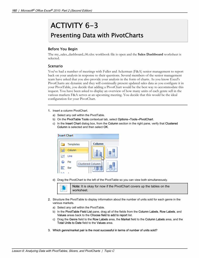
ACTIVITY 6-3Presenting Data with PivotCharts

Before You BeginThe my_sales_dashboard_06.xlsx workbook file is open and the Sales Dashboard worksheet isselected.

ScenarioYou've had a number of meetings with Fuller and Ackerman (F&A) senior management to reportback on your analysis in response to their questions. Several members of the senior managementteam have asked that you also provide your analysis in the form of charts. As you know Excel'sPivotCharts are dynamic and they will continually present updated sales data as you configure it inyour PivotTable, you decide that adding a PivotChart would be the best way to accommodate thisrequest. You have been asked to display an overview of how many units of each genre sell in thevarious markets F&A serves at an upcoming meeting. You decide that this would be the idealconfiguration for your PivotChart.

1. Insert a column PivotChart.a) Select any cell within the PivotTable.b) On the PivotTable Tools contextual tab, select Options→Tools→PivotChart.c) In the Insert Chart dialog box, from the Column section in the right pane, verify that Clustered

Column is selected and then select OK.

d) Drag the PivotChart to the left of the PivotTable so you can view both simultaneously.

Note: It is okay for now if the PivotChart covers up the tables on theworksheet.

2. Structure the PivotTable to display information about the number of units sold for each genre in thevarious markets.a) Select any cell within the PivotTable.b) In the PivotTable Field List pane, drag all of the fields from the Column Labels, Row Labels, and

Values areas back to the Choose field to add to report list.c) Drag the Genre field to the Row Labels area, the Market field to the Column Labels area, and the

Total Units to Date field to the Values area.

3. Which genre/market pair is the most successful in terms of number of units sold?A: The romance genre in the NA market.



Do Not D

uplicate

or Dist

ribute

4. Filter out the romance genre to get a better understanding of how the other genres compare to eachother.a) On the PivotChart, select the Genre down arrow.

b) Uncheck the Romance check box and select OK.c) Verify that Excel filtered the Romance genre out of both the PivotChart and the PivotTable.

5. Use the PivotChart to compare the average number of units sold for the remaining genres.a) On the PivotChart, right-click Sum of Total Units to Date and select Value Field Settings.b) In the Value Field Settings dialog box, from the Summarize Values By tab, select Average and then

select OK.c) Verify that both the PivotChart and the PivotTable display the average number of units sold for the

remaining genres.

6. Clear the filter on the Genre field and drag the PivotChart to the empty space between the standardcharts and the tables on the worksheet.




Do Not D

uplicate

or Dist

ribute

TOPIC DFilter Data by Using SlicersThe ability to filter your PivotTables enables you to drill down into your raw data to view the finedetail that lies within. As you likely have many questions to ask of your data, it can quickly becometedious to have to open drop-down menus, determine what items are filtered out, clear the filtering,and then re-filter your data to find the next answer. This is especially true if data analysis is one ofyour key functions. If you fall into this category of Excel users, you'll likely appreciate the ability toquickly and easily re-filter your PivotTables on any number of fields. In addition, the ability toquickly view the filters applied to the current dataset could come in handy if you're returning to aworksheet after having not worked in it for a while.In short, you need some type of tool that gives you a high level of control over PivotTable filtering,one that is easy to work with and easy to interpret regardless of how many filters you apply to yourPivotTables. Excel 2010 includes such a tool. Gaining an understanding of how this feature workswill give you a greater level of control over your PivotTable filtering and the peace of mind ofknowing that you have filtered your data in precisely the manner you meant you.

SlicersSlicers are PivotTable filtering tools that you can link to various PivotTables in your worksheets. Youcan create a slicer out of any of the fields associated with a PivotTable, and then you can use thoseslicers to filter each field by any of its unique entries. Although a slicer is typically associated with asingle PivotTable, you can link slicers to multiple PivotTables; this is typically done for PivotTablesthat are associated with the same raw dataset. This can be handy, for example, if you want to createmultiple versions of the same PivotTable, create a unique structure for each to answer variousquestions about your data, and then filter them by the same criteria simultaneously.Each unique value in a field appears as a separate button on the associated slicer. By default, slicerbuttons appear highlighted in blue when the filter is inactive, meaning the associated value willappear in the PivotTable. When the filter is active, meaning the value has been removed from thePivotTable, the button appears white. When you first create a slicer, all filters are inactive, so all ofthe buttons are highlighted in blue. Selecting a slicer button activates all of the other filters, meaningonly the value you selected will appear in the table. This may, at first, seem counterintuitive, but itmakes sense when you think about it in this way: Selecting a button displays the associated value in aPivotTable. To select multiple slicer buttons simultaneously, press and hold down the Ctrl key whilemaking your selections. Selecting the Clear Filter button deactivates all filters on a slicer, meaningall values will appear in the PivotTable.Slicer buttons may also appear slightly grayed-out. Excel does this when some active filter hasremoved the associated values from view. Grayed-out slicer buttons are inactive, as you cannot filteron values that do not appear in the PivotTable. Clearing the filter that is suppressing the values fromview will reactivate the associated slicer button(s).The default slicer formatting is blue and white but you can customize the display of slicers to matchyour worksheet formatting. You can place slicers anywhere on your worksheets or resize them asyou like. You can even place copies of slicers in multiple locations. The original slicer and the copiesremain linked, so whatever you do to one affects the others. This is true only of filtering tasks, notvisual formatting.


Lesson 6: Analyzing Data with PivotTables, Slicers, and PivotCharts | Topic D

Slicers

Do Not D

uplicate

or Dist

ribute

Figure 6-10: Use slicers to quickly and easily apply multiple filters to your PivotTables.

Note: For information on an alternate way to filter PivotTables, watch the LearnTO Add aReport Filter to an Excel PivotTable presentation from the LearnTO tile on theLogicalCHOICE Course screen.

The Insert Slicers Dialog BoxYou use the Insert Slicers dialog box to create slicers out of the various fields in your PivotTables.Each field appears as a check box option in the dialog box. To create a slicer out of a particularfield, check the associated check box. You can access the Insert Slicers dialog box from thePivotTable Tools contextual tab by selecting Options→Sort & Filter→Insert Slicer.

Figure 6-11: The Insert Slicers dialog box enables you to create slicers out of any PivotTablefield.



You may want to showLearnTO Add a ReportFilter to an ExcelPivotTable from theLogicalCHOICE Coursescreen or have studentsnavigate out to theCourse screen andwatch it themselves as asupplement to yourinstruction. If not, pleaseremind students to visitthe LearnTOs for thiscourse on theirLogicalCHOICE Coursescreen after class forsupplementalinformation andadditional resources.The Insert Slicers DialogBox

Do Not D

uplicate

or Dist

ribute

The Slicer Tools Contextual TabYou can access the commands you will use to work with PivotTable slicers on the Slicer Toolscontextual tab. The Slicer Tools contextual tab appears when you select a slicer and disappearswhen you select any non-slicer object. If you select multiple slicers simultaneously, some of thecommands on the Slicer Tools contextual tab remain active and others become deactivated. Forexample, you can typically resize or apply formatting to multiple slicers at the same time, but youcan only manage slicer connections one at a time.

Figure 6-12: The Slicer Tools contextual tab.

The following table describes the types of commands you will find in the command groups on theSlicer Tools contextual tab.

Slicer Tools ContextualTab Group


Slicer Renaming slicers, accessing slicer options, and managing slicerconnections to PivotTables.

Slicer Styles Applying formatting to slicers.

Arrange Configuring the arrangement of slicers on screen. You can use thecommands in this group to order slicers from front to back, alignslicers with other objects, and rotate the display of slicers.

Buttons Modifying the size and alignment of slicer buttons. Changes youmake here can also affect the size of the slicers themselves.

Size Modifying the size of slicers. Changes you make here can also affectthe display of slicer buttons.

The PivotTable Connections Dialog BoxYou can use the PivotTable Connections dialog box to manage slicer connections. All PivotTablesthat are associated with the same raw dataset can share slicers. These shared slicers affect allPivotTables that share them, so what you filter in one PivotTable is filtered in all PivotTables thatshare the slicer. It is important to note that PivotTables that are associated with the same rawdataset do not have to share slicers. You can create unique slicers for each PivotTable that filter thesame fields independently on each PivotTable. It is only the slicers that you connect to multiplePivotTables that will affect those PivotTables simultaneously. You can access the PivotTableConnections dialog box from the Slicer Tools contextual tab by selectingOptions→Slicer→PivotTable Connections.



The Slicer ToolsContextual Tab

The PivotTableConnections Dialog Box

Do Not D

uplicate

or Dist

ribute

Figure 6-13: Use the PivotTable Connections dialog box to manage slicer connections.

Access the Checklist tile on your LogicalCHOICE course screen for referenceinformation and job aids on How to Insert and Work with Slicers.



Do Not D

uplicate

or Dist

ribute

ACTIVITY 6-4Filtering Data by Using Slicers

Before You BeginThe my_sales_dashboard_06.xlsx workbook file is open, and the Sales Dashboard worksheet isselected.

ScenarioThere has been even more of an increase in demand for analysis on the raw sales data in your salesdashboard workbook. With requests for information coming it at an ever-faster pace, you'd like tofind a faster way to filter your PivotTable so you can provide answers to questions more quickly andeasily. You feel that adding slicers would be the best approach. You decide to add slicers for each ofthe fields you commonly filter on and use the slicers to filter the PivotTable to answer the followingquestions from senior managers:• How many romance print books has author 1029 sold in the APAC market?• Of author 1056's NA electronic format sales for fantasy and science fiction, what percentage is

from the science fiction genre?

1. Insert slicers for the commonly filtered fields.a) Select any cell within the PivotTable.b) From the PivotTable Tools contextual tab, select Options→Sort & Filter→Insert Slicer.c) In the Insert Slicers dialog box, check the Author, Title, Genre, Format, and Market check boxes.d) Select OK.

2. Reposition the slicers to the right of the PivotTable on the Sales_Dashboard worksheet.



As an alternative to step1b, remind the studentsthat they can use theInsert Slicer commandthey added to the ribbonin Lesson 1.Inform the students thatit's not importantprecisely how the slicersare arranged or placedon the worksheet. Theymay even have torearrange them as theywork, which issomething they mightencounter in the realworld.

Do Not D

uplicate

or Dist

ribute

3. Select any cell within the PivotTable and then drag all fields from the various areas back to the Choosefields to add to report list.

4. Structure and filter the PivotTable to answer the question "How many romance print books has author1029 sold in the APAC market?"a) Drag the Author field to the Row Labels area, the Market field to the Column Labels area, and the

Total Units to Date field to the Values area.b) On the Author slicer, scroll down and select 1029.c) On the Format slicer, select Print and, on the Genre slicer, select Romance.

5. How many romance print books has author 1029 sold in the APAC market?A: 1,935,355

6. Clear all filters by selecting the Clear Filter button on the Format, Genre, and Author slicers.

7. Structure and filter the PivotTable to answer the question "Of author 1056's NA electronic format salesfor fantasy and science fiction, what percentage is from the science fiction genre?"a) Select any cell within the PivotTable, and then drag the Genre field to the Row Labels area, placing

it below the Authors field.

b) On the Author slicer, select 1056 and, on the Format slicer, select Electronic.



Do Not D

uplicate

or Dist

ribute

c) On the Genre slicer, select Fantasy, press and hold Ctrl, and then select SF.d) Right-click any data cell within the PivotTable and select Show Values As→% of Column Total.

8. Of author 1056's electronic fantasy and science fiction book sales in the NA market, what percentage isrepresented by science fiction sales?A: 31.42 percent




Do Not D

uplicate

or Dist

ribute

SummaryIn this lesson, you used PivotTables, PivotCharts, and slicers to analyze and present your data. Theability to crunch and re-crunch your numbers, ask incredibly detailed questions of your data, presentyour results in an easily digestible manner, and do it all over again without affecting your raw dataputs the power of information right in the palm of your hand. As the volume of data, and the speedat which organizations generate it, continues to grow, your ability to mine actionable intelligencefrom it becomes increasingly critical and can give you the competitive edge to succeed.

How do you see PivotTables and PivotCharts helping you with your regular tasks?

A: Answers may vary, but most students will find the power and flexibility in these tools to be a hugebenefit over manually entering formulas and then re-entering them to find answers to a differentquestion.

When might you use slicers?

A: Answers may vary, but users who often analyze complex datasets with a large number of fields willlikely find quick access to filtering tools and easy-to-read filter indicators a huge help when looking formultiple answers to a variety of questions about their data.



Lesson 6: Analyzing Data with PivotTables, Slicers, and PivotCharts |


Do Not D

uplicate

or Dist

ribute

Do Not D

uplicate

or Dist

ribute

Course Follow-UpCongratulations! You have completed the Microsoft® Office Excel® 2010: Part 2 (Second Edition) course.You have successfully customized the Excel environment to suit your needs, and used advancedformulas and analysis tools to extract actionable organizational intelligence from Excel data.To gain a competitive edge in today's market, decision makers need to have a keen understanding ofwhat's happening within their organizations. They need to be able to ask specific questions and getspecific answers even when sifting through massive amounts of data. Becoming proficient atengaging your data in an ongoing dialog to find these answers means you'll be able to provide thedecision makers within your organization with the intelligence they need to keep you ahead of thecompetition. The more you know about Excel's analysis tools and formula and function syntax, thebetter you'll be able to analyze and examine your raw data to find the nuanced patterns andopportunities that could mean the difference between running with the pack and staying one stepahead of everyone else.

What's Next?Microsoft® Office Excel® 2010: Part 3 (Second Edition) is the next course in this series. In that course,you will build upon the skills you have acquired by automating a number of Excel tasks, applyingconditional logic to your analysis, auditing and troubleshooting your workbooks to identify andcorrect errors, and presenting your analysis with advanced chart features. You are also encouragedto explore Excel further by actively participating in any of the social media forums set up by yourinstructor or training administrator through the Social Media tile on the LogicalCHOICE Coursescreen.


Course Follow up

Do Not D

uplicate

or Dist

ribute

Do Not D

uplicate

or Dist

ribute

Financial FunctionsFinance and accounting professionals are most likely to use Excel's financial functions.These specialized functions are useful for calculating a variety of financial values, such aspayments, interest, and investment values over time. The following are overviews of someof the more commonly used Financial functions not directly covered in the course.

Note: These function overviews assume some prior knowledge of finance.

The IPMT FunctionSyntax: =IPMT(rate, per, nper, pv, [fv], [type])Description: This function returns the interest payment due for a particular period on aninvestment or a loan with regular payments and a fixed interest rate. Here is a breakdown ofthe function's syntax.Required arguments:• rate: The interest rate per period. It's important to be specific about the payment period

here. If your interest rate is 10 percent and payments are made monthly, the rate valueshould be 10 percent divided by 12, or 0.10/12. If payments are annual, the rate valuewould simply be 10 percent, or 0.10.

• per: The period for which you wish to calculate the interest. Take note that this is not arange of dates or a specific date, but rather the payment number itself. So if paymentsare monthly on a four-year investment, the per value will have to be somewhere between1 and 48. If you're calculating the interest for the first month of year 2, the per value is13.

• nper: The total number of payments for the investment. For example, if payments aremonthly on a five-year investment, the nper value is 60. Literally, this is the number ofpayment periods for the duration of the investment.

• pv: The principal, or lump-sum, value. This is the present value of all remainingpayments.

Note: For all arguments in the IPMT function, use positive numbers for any moneyyou must pay out, and use positive numbers for any money you take in.

Optional arguments:• fv: The future value of the investment after all payments have been made. If you do not

enter a value for the fv argument, Excel treats it as zero. This may be easier to think of interms of a loan. Typically, you are interested in values associated with paying a loan offin full, so the final, or future, value is 0.

• Type: Designates when payments are due within a particular period. This argument canhave one of two values: 0 or 1. A value of 0 indicates payments are due at the end of thegiven period, for example, the last day of the month. A value of 1 indicates payments aredue at the beginning of the period, for example, the first day of the year. If you do notenter a value, Excel treats it as 0.

A

Do Not D

uplicate

or Dist

ribute

Example: In the following example how much interest a borrower would owe in the first month ofthe second year of a five-year, $10,000 loan is being calculated. Payments are due at the end of eachmonth.

If you were making the same calculation from the bank's perspective, you would have entered -$10,000 for the principal, as you would have paid the money out to the borrower. Excel wouldreturn $62.50, not -$62.50, because the interest payment would be owed to you from the borrower.The value 13 is entered for the per argument because the first month of the second year representsthe 13th payment period.

The PPMT FunctionSyntax: =PPMT(rate, per, nper, pv, [fv], [type])Description: The PPMT function calculates the amount owed against the principal for a particularperiod on an investment or a loan with regular payments and a fixed interest rate. The arguments forthe PPMT function are exactly the same as those for the IPMT function. If you add the valuesreturned for the same period of the same loan by the IPMT function and the PPMT function, youwill calculate the total payment, less any fees, for the period.Example: This is what the PPMT function would return for the aforementioned example for theprincipal payment due in the same period.

The NPV FunctionSyntax: =NPV(rate, value1, [value2], ..., [value254])Description: The NPV function calculates the net present value of an asset or an investment giventhe estimated or known future cash flows and the discount rate per period. In the function's syntax,rate is the discount rate per period, and the valueX arguments represent the future cash flows. Forthis function, the cash flow, or value argument, period must be fixed and the cash flows must occurat the end of each period.

Note: The NPV function does not take into account the initial cost of the investment, or thecash flow at Time 0. You must subtract this from the value returned by the NPV functionmanually to calculate the actual increase or decrease in net value from the investment.

Example: In the following example, assume an annual discount rate of 9 percent and the givenestimated cash flows.


Appendix A : Financial Functions |

Do Not D

uplicate

or Dist

ribute

Notice that the initial cost is not included in the function, this is not factored in. To calculate thetrue NPV of the investment, you must subtract the initial cost of the investment from the valuereturned by the NPV formula. In this case, the NPV for the investment is $29,589.21.

The FV FunctionSyntax: =FV(rate, nper, pmt, [pv], [type])Description: This function calculates the future value of an investment with fixed, periodicpayments and a fixed interest rate. Here is a breakdown of the function's syntax.Required:• rate: The interest rate per period. As with some of the other financial functions, it's important to

be specific about the period here. If the interest rate is 10 percent and payments are mademonthly, the rate value should be 10 percent divided by 12, or 0.10/12. If payments are annual,the rate value would simply be 10 percent, or 0.10.

• nper: The number of periods from now for which you wish to calculate the future value. Makesure the periods for this argument are the same as those used in the rate argument.

• pmt: the payment made each period. For example, if you invest $200 a month from yourpaycheck toward a retirement investment for 20 years, the pmt value should be 200 and the npervalue should be 240 (12 months × 20 years).

Note: Although the pmt argument is considered to be required, that's not exactly true. Youcould also use the FV function to calculate the future value of a lump-sum investment. Forexample, if you put $10,000 in a fixed-rate investment, without making additional periodiccontributions, you could simply enter 10000 in the pv argument, and leave the pmt argumentblank. The FV function would then return the future value of that lump sum if it satuntouched in the same investment.

Optional:• pv: The present value of the investment. Use this argument to determine the future value of a

one-time, lump-sum investment into a fixed-rate asset. Or, you can use this in addition to thepmt argument to determine the future value of an investment in which you already have money,but plan to add to on a regular basis over time.

• type: Designates when payments are made within a particular period. This argument can haveone of two values: 0 or 1. A value of 0 indicates payments are made at the end of the givenperiod, for example, the last day of the month. A value of 1 indicates payments are made at thebeginning of the period, for example, the first day of the year. If you do not enter a value, Exceltreats it as 0.

Example: In the following example, assume the investor put $10,000 into an investment with anannual fixed-rate of return of 8 percent. Also assume the investor plans to contribute another $1,500each month for 30 years with payments made at the end of each month.



Do Not D

uplicate

or Dist

ribute



Do Not D

uplicate

or Dist

ribute

Date and Time FunctionsExcel's date and time functions are often used by business analysts, human resourcesprofessionals, and project managers, who all frequently deal with scheduling and analyzingdata for particular periods of time. But there are also a couple of handy functions for simplyentering the current date or time. The following are overviews of some of the morecommonly used in date and time functions.

The TODAY FunctionSyntax: =TODAY()Description: This function enters the current date in a cell. This function has no arguments.Simply enter it into a cell to return the current date in whatever date format you haveapplied to the cell. You can use the value returned by this function to perform othercalculations related to durations of time.Example: In the following example, the TODAY function is entered into two cells, onewith the default date format and one with a different format applied.

The NOW FunctionSyntax: =NOW()Description: Like the TODAY function, this function has no arguments; it simply returnsthe current date and time in the cell you enter in into. You can use the value returned by thisfunction to perform other calculations related to durations of time.

Note: When you enter the NOW function in a cell, Excel automatically formats the cellwith a custom cell format used to accommodate both the date and the time. Here is theformat: m/d/yyyy h:mm. Although the format displays only a single m for month and asingle d for day, dates will appear in cells with both numbers for months and dates thatcontain two digits. If you alter the format to a different date or time format, you willalter the value in the cell.

Example: In the following example, the NOW function is entered in cell A1.

B

Do Not D

uplicate

or Dist

ribute

The DATE functionSyntax: =DATE(year, month, day)Description: The DATE function returns the serial number for the date entered in the arguments.This is because Excel uses a serial number system to represent dates and times. January 1, 1900 isrepresented by the number 1. Each day after that increases by one whole number. So, January 12,1900 is represented by the number 12. This is how Excel is able to display dates in a number ofdifferent formats as the underlying serial number is always the same. Although the DATE functiontechnically returns the specified date's serial number, it displays the date in whatever date format isapplied to your worksheet cells.

Note: Times are represented by decimal places that follow the date's whole number andrepresent the number of hours and minutes that have passed in a day up to the desired orcalculated time.

In the DATE function's syntax, the year argument is the four-digit year you wish to enter, themonth argument is the calendar month represented in numbers from 1 to 12, and the day argumentis the desired date. You use the DATE function largely to make calculations using other date andtime functions, as using plain text or simply entering the date and time values can return errors.Example: In the following example, the DATE function has been used to return the date September27, 2003, and a specific date format has been applied to the cell.

The NETWORKDAYS FunctionSyntax: =NETWORKDAYS(start_date, end_date, [holidays])Description: The NETWORKDAYS function returns a count of the number of work days betweentwo specific dates. You would use this function, for example, to determine how many working daysyou'll have to complete a project from now until a specific date in the future, or to calculate howmuch of a particular benefit employees have accrued. In the function's syntax, the start_dateargument is the first date of the range for which you wish to count the number of work days. Theend_date argument is the last day of the range. The optional holidays argument allows you toexclude known holidays so they are not counted as work days. The NETWORK days functionautomatically excludes weekends from the calculation.Example: In the following example, the number of working days are being counted in a project,which starts on June 12, 2008 and ends on December 15, 2008. The project team will all be off onThanksgiving and the day after. The cells in the range B1:B4 have all been entered using the DATEfunction.


Appendix B : Date and Time Functions |

Do Not D

uplicate

or Dist

ribute


Appendix B : Date and Time Functions |

Do Not D

uplicate

or Dist

ribute

Do Not D

uplicate

or Dist

ribute

Working with GraphicalObjectsAppendix IntroductionAlthough data is king in Excel, there are a number of reasons you may need to add graphicalobjects, outside of charts or PivotCharts, to your worksheets. You may want to simplyenhance the visual appeal of your worksheets, or you may wish to include some type of"info-graphic" that simply can't be created with a chart. Perhaps you want to include yourcompany logo in a visible location when sharing your screen with potential clients. Or, youmay wish to include screenshots of relevant computer applications or websites whenpresenting related information.Whatever the case, at some point you'll likely need to insert graphical support for the data inyour workbooks. Excel 2010 provides you with a number of tools for inserting, modifying,and even editing a variety of graphical objects that can not only enhance the visual appeal ofa document, but can also serve as interactive data objects. Understanding what these objectsare, how they work, and how you can integrate them with your data can help you elevateyour workbooks to a new level of sophistication.

C

Do Not D

uplicate

or Dist

ribute

TOPIC AInsert Graphical ObjectsBefore you can use graphical objects to enhance the visual appeal of your workbooks or presentyour data with greater impact, you must first be able to insert them into your worksheets. Excel2010 provides you with a variety of tools and commands that enable you to add a variety ofgraphical objects to your worksheets. Understanding the differences among the various types ofgraphical objects and the various methods for inserting them is a key first step in using graphicalobjects to enhance your workbooks.

Graphical ObjectsThere are five basic types of graphical objects that you can insert into your workbooks: pictures, clipart, shapes, SmartArt, and screenshots. Each of these is suited to particular purposes. It's importantto understand that these objects, much like charts, are separate data objects that lie on top ofworksheets; you do not insert them in cells. All of these graphical objects can be resized, modified,and moved. Some of them can also contain text or display the content of worksheet cells. You canaccess the commands for inserting graphical objects in the Illustrations group on the Insert tab.

Figure C-1: Graphical objects enable you to add appeal to your worksheets and present datavisually.

The following table describes each of the types of graphical objects in some detail.

Graphical ObjectType

Description

Pictures These are image files created outside of Excel, such as images from digitalcameras, pictures downloaded from the web, or graphics and art saved asimage files. Excel 2010 supports a variety of common image file formats.

Clip art Simple artwork graphics or images that are pre-loaded into Excel or that aredownloaded from Office.com. Clip art objects behave differently dependingon the type of graphical object you select, but they are all still genericallyreferred to as clip art.


Appendix C : Working with Graphical Objects | Topic A

Do Not D

uplicate

or Dist

ribute

Graphical ObjectType

Description

Shapes Simple graphical objects, such as circles, squares, rectangles, text callouts, andarrows, that are generated within Excel and that you manually draw on yourworksheets. Excel 2010 comes loaded with a wide variety of shapes. Shapescan also display text or the contents of worksheet cells.

SmartArt Pre-configured graphics that you can use as graphical representations of textualcontent. You will typically use SmartArt to represent processes, procedures,cycles, or hierarchies. Common uses of SmartArt include creatingorganizational charts and representing sales or business cycles. As with shapes,you can use SmartArt to display text, but you cannot link cell content toSmartArt graphics.

Screenshots Images taken from the current display of your computer monitor. You capturethese images directly within Excel, which can be of either entire windows orparticular regions of your screen. Excel enables you to screen capture anycurrently open windows that are not minimized.

The Clip Art PaneYou will use the Clip Art pane to insert clip art objects, or clips, into your workbooks. From here,you can enter search criteria for the clips you wish to use, select from among a variety of mediatypes, and insert the desired clips. Typically, clips will be in the form of simple illustrations orphotographs. You can also search for and insert audio and simple video clips, although you willlikely need to play these back in a separate application. You can access the Clip Art pane byselecting Insert→Illustrations→Clip Art.



Do Not D

uplicate

or Dist

ribute

Figure C-2: The Clip Art pane.

The following table describes the functions of the various Clip Art pane elements.

Clip Art Pane Element Use This To

Search for field Enter search criteria for the desired clip art.

Go button Execute a search for clip art.

Results should be drop-down menu Select the desired media type for your clip art.

Include Office.com content checkbox

Decide whether Excel will search for clip art only onyour computer or on your computer and fromOffice.com. When you install Excel, a library of clip artis installed along with it.

Search results Review search results and select the desired clip art.

Find more at Office.com link Navigate to Office.com to search for a wide variety ofavailable clip art.

Hints for finding images link Open Excel Help to an article specific to searching forand adding clip art.



Do Not D

uplicate

or Dist

ribute

The Shapes GalleryYou will select the particular shapes you wish to add to your worksheets by using the Shapesgallery. The Shapes gallery is divided into a series of nine categories of related shape types. Theseinclude simple lines and arrows, basic geometric shapes, flowchart elements, and text callout boxes.Shapes you have recently used in your workbooks appear in the Recently Used Shapes section atthe top of the Shapes gallery. You can access the Shapes gallery by selectingInsert→Illustrations→Shapes.

Figure C-3: The Shapes gallery.

The Screenshot CommandThe Screenshot command enables you to capture an image from an open application on yourcomputer. You can capture either an entire application window or a particular region of the screen.



Do Not D

uplicate

or Dist

ribute

The Screenshot tool enables you to screen capture open applications that are not minimized to thetask bar. When you select the Screenshot command, Excel opens the Available Windows gallery,from which you can select an open application to capture. This method captures an image of theentire window of the selected application. To capture only a portion of the application window,select the Screen Clipping command from the bottom of the Available Windows gallery. Excelthen activates the Screen Clipping tool, enabling you to select the particular region of your screenthat you wish to capture. This allows you to select the particular region of your screen that you wishto capture. The Screen Clipping tool also allows you to capture screenshots of your desktop, whichis not possible from the Available Windows gallery. You cannot capture an image of Excel fromwithin Excel. You can access the Screenshot tool by selecting Insert→Illustrations→Screenshot.

Figure C-4: The Screenshot command.

Access the Checklist tile on your LogicalCHOICE course screen for referenceinformation and job aids on How to Insert Graphical Objects.



Do Not D

uplicate

or Dist

ribute

TOPIC BModify Graphical ObjectsInserting graphical objects is a great way to enhance the visual appeal and impact of yourworkbooks. However, many of the raw images or basic shapes you insert may not suit yourparticular needs. For instance, you may need to ensure that all shapes adhere to your organization'sbranding guidelines. Or you may want to remove distracting background elements from images tofocus your audience's attention on only the most important aspects of pictures. Whatever thereason, taking the time to gain the foundational knowledge needed to modify and edit your graphicalobjects will give you the flexibility you need to ensure your images deliver the proper message andhave the desired impact.

Note: While there are no formal activities for this lesson, a sample data file has been providedthat you can use to practice adding shapes and connecting them to cell data in the C:\091019Data\Appendix E folder. Use the graphic_objects.xlsx file to practice adding,modifying, and connecting data to shapes; one has been included in the workbook as anexample. You can also practice adding images or SmartArt as well. A sample solution file hasbeen provided in the C:\091019Data\Appendix E\solutions folder.

Pictures and DrawingsThere is an important distinction to understand before you modify the graphical objects in yourworkbooks. With the exception of SmartArt, although there are four types of graphical objects inExcel, pictures, clip art, shapes, and screenshots, Excel recognizes only two types of images in termsof editing and modifying graphical objects: pictures and drawings.

Note: Although, technically, the individual elements of a SmartArt graphic are the same asshapes, SmartArt has a separate set of tools that you will use to modify your SmartArt graphics.

In terms of modifying graphical objects, Excel considers pictures, screenshots, and some clip art tobe pictures, whereas it considers shapes and some other clips to be drawings. Each has its ownunique set of tools for working with and modifying the various types of graphical objects. In generalterms, the clip art images you can search for by checking Illustrations in the Results should bedrop-down menu of the Clip Art pane are considered drawings. On the other hand, clip art imagesyou search for by checking Photographs are considered pictures.

Figure C-5: Excel draws a distinction between drawings and pictures.


Appendix C : Working with Graphical Objects | Topic B

Do Not D

uplicate

or Dist

ribute

The Picture Tools Contextual TabExcel displays the Picture Tools contextual tab when you select a graphical object it considers to bea picture. The Picture Tools contextual tab contains only one tab, the Format tab, which displaysthe tools and commands you will use to edit, modify, and add effects to the pictures in yourworkbooks.

Figure C-6: The Picture Tools contextual tab.

The Image EditorThe Adjust group on the Format tab of the Picture Tools contextual tab contains a set ofcommands and tools sometimes referred to collectively as the image editor. These commands andtools enable you to perform image editing tasks, such as adjusting the brightness, contrast, orsharpness of a picture, that you might otherwise need a separate application to perform.

Figure C-7: The Adjust group's imaging editing tools.

The following table describes the type of image-correction and -modification tasks you can performby using the tools and commands available in the image editor.

Image Editor Command/Tool Use This To

Remove Background tool Remove unwanted background elements from a picture. TheRemove Background tool will attempt to guess at the mainsubject of an image and remove all other backgroundelements. You can also manually select which regions of animage Excel will keep and which elements it will remove.

Corrections command Adjust the sharpness, brightness, or contrast of an image.

Color command Adjust the color tone or saturation of an image, recolor animage, or select a particular color to make transparent in animage.

Artistic Effects command Apply a particular artistic effect to an image, such as making animage look like a pencil sketch, adding a blur effect, adding apixelated effect, or turning a color image into a black-and-white image.

Compress Picture command Reduce the overall file size of your Excel workbook bycompressing the images it contains.

Change Picture command Replace a picture with another image file.

Reset Picture command Remove any formatting changes you've made to a picture.



Do Not D

uplicate

or Dist

ribute

The Drawing Tools Contextual TabExcel displays the Drawing Tools contextual tab when you select a graphical object it considers tobe a drawing. The Drawing Tools contextual tab contains only one tab, the Format tab, whichdisplays the tools and commands you will use to edit, modify, and add effects to the drawings inyour workbooks.

Figure C-8: The Drawing Tools contextual tab.

The Format tab on the Drawing Tools contextual tab is divided into five command groups. Eachof these groups displays functionally related commands for working with drawings in Excel.

Format Tab Group Contains Commands For

Insert Shapes Inserting additional shapes, changing the outline (shape) of ashape, and inserting text boxes.

Shape Styles Applying a variety of pre-configured or custom styles to drawings.

WordArt Styles Applying a variety of pre-configured or custom styles to text youadd to drawings.

Arrange Changing the placement of drawings on worksheets, arrangingmultiple drawings front-to-back, grouping drawings together, androtating drawings.

Size Modifying the size of drawings.

The Selection and Visibility PaneAlthough you can use the commands on the Picture Tools or the Drawing Tools contextual tabsto arrange images front to back on your worksheets, Excel 2010 includes a tool that makes doing soeasier: the Selection and Visibility pane. The Selection and Visibility pane enables you to easilyview the front-to-back order of graphical objects on your worksheets, view which objects aregrouped together, change the order of objects and groups (and individual objects within groups),and hide from view or display any of the graphical objects on your worksheets.It may not appear as such when objects are separated from each other, but all objects on aworksheet are arranged in a front-to-back order as if each exists on its own plane. This fact becomesevident, however, when you overlap objects on screen. Objects that are in front of other objects willobscure the view of the objects behind them. Objects appear in the Selection and Visibility panefrom top to bottom as they appear on the worksheet from front to back. In other words, the objectat the top of the Selection and Visibility pane is in front of all other objects on the worksheet.When you group objects together, they behave as one independent object that you can move,arrange, resize, or modify collectively. You are, however, able to select individual objects within agroup to perform modifications on it separate from the group. Grouped objects appear in theSelection and Visibility pane in a hierarchical fashion with the group existing at the same level asother independent objects, and the objects in the group appearing one level down in the hierarchywithin the group.



Do Not D

uplicate

or Dist

ribute

Figure C-9: The Section and Visibility pane.

The following table describes the functions of the various elements of the Selection and Visibilitypane.

Selection and Visibility PaneElement

Description

Shapes on this Sheet section Displays the order of all objects and groups on a worksheet aswell as the order in which individual objects appear within agroup.

Eye buttons Enable you to hide or show any object or group.

Show All button Turns on the display of all objects and groups on a worksheet.

Hide All button Turns off the display of all objects and groups on a worksheet.

Bring Forward and SendBackward buttons

Enable you to move objects or groups up or down in theSelection and Visibility pane, which changes their order on theworksheet.

Access the Checklist tile on your LogicalCHOICE course screen for referenceinformation and job aids on How to Modify Graphical Objects.



Do Not D

uplicate

or Dist

ribute

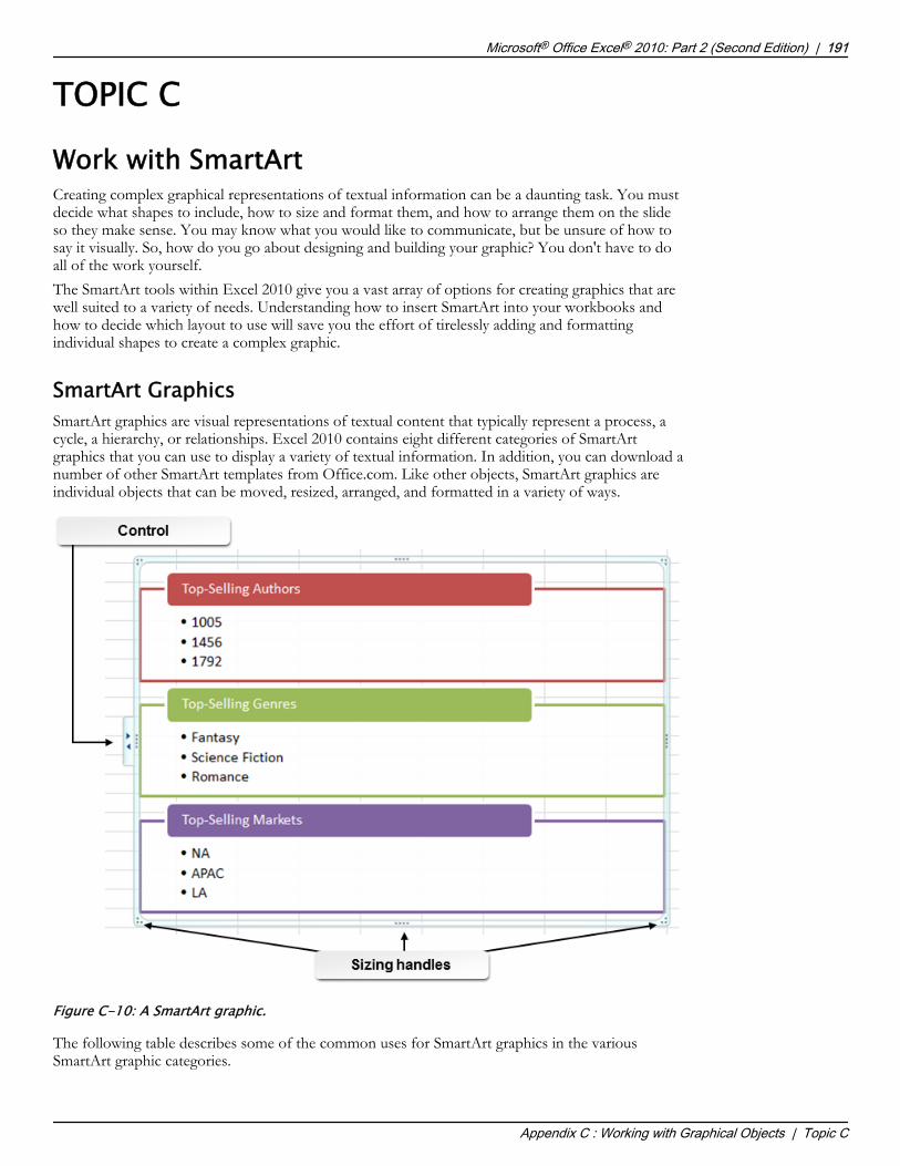
TOPIC CWork with SmartArtCreating complex graphical representations of textual information can be a daunting task. You mustdecide what shapes to include, how to size and format them, and how to arrange them on the slideso they make sense. You may know what you would like to communicate, but be unsure of how tosay it visually. So, how do you go about designing and building your graphic? You don't have to doall of the work yourself.The SmartArt tools within Excel 2010 give you a vast array of options for creating graphics that arewell suited to a variety of needs. Understanding how to insert SmartArt into your workbooks andhow to decide which layout to use will save you the effort of tirelessly adding and formattingindividual shapes to create a complex graphic.

SmartArt GraphicsSmartArt graphics are visual representations of textual content that typically represent a process, acycle, a hierarchy, or relationships. Excel 2010 contains eight different categories of SmartArtgraphics that you can use to display a variety of textual information. In addition, you can download anumber of other SmartArt templates from Office.com. Like other objects, SmartArt graphics areindividual objects that can be moved, resized, arranged, and formatted in a variety of ways.

Figure C-10: A SmartArt graphic.

The following table describes some of the common uses for SmartArt graphics in the variousSmartArt graphic categories.


Appendix C : Working with Graphical Objects | Topic C

Do Not D

uplicate

or Dist

ribute

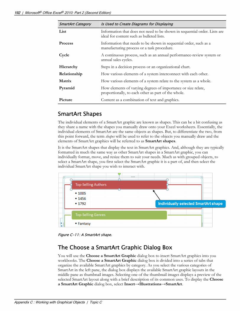
SmartArt Category Is Used to Create Diagrams for Displaying

List Information that does not need to be shown in sequential order. Lists areideal for content such as bulleted lists.

Process Information that needs to be shown in sequential order, such as amanufacturing process or a task procedure.

Cycle A continuous process, such as an annual performance-review system orannual sales cycles.

Hierarchy Steps in a decision process or an organizational chart.

Relationship How various elements of a system interconnect with each other.

Matrix How various elements of a system relate to the system as a whole.

Pyramid How elements of varying degrees of importance or size relate,proportionally, to each other as part of the whole.

Picture Content as a combination of text and graphics.

SmartArt ShapesThe individual elements of a SmartArt graphic are known as shapes. This can be a bit confusing asthey share a name with the shapes you manually draw onto your Excel worksheets. Essentially, theindividual elements of SmartArt are the same objects as shapes. But, to differentiate the two, fromthis point forward, the term shapes will be used to refer to the objects you manually draw and theelements of SmartArt graphics will be referred to as SmartArt shapes.It is the SmartArt shapes that display the text in SmartArt graphics. And, although they are typicallyformatted in much the same way as other SmartArt shapes in a SmartArt graphic, you canindividually format, move, and resize them to suit your needs. Much as with grouped objects, toselect a SmartArt shape, you first select the SmartArt graphic it is a part of, and then select theindividual SmartArt shape you wish to interact with.

Figure C-11: A SmartArt shape.

The Choose a SmartArt Graphic Dialog BoxYou will use the Choose a SmartArt Graphic dialog box to insert SmartArt graphics into youworkbooks. The Choose a SmartArt Graphic dialog box is divided into a series of tabs thatorganize the available SmartArt graphics by category. As you select the various categories ofSmartArt in the left pane, the dialog box displays the available SmartArt graphic layouts in themiddle pane as thumbnail images. Selecting one of the thumbnail images displays a preview of theselected SmartArt layout along with a brief description of its common uses. To display the Choosea SmartArt Graphic dialog box, select Insert→Illustrations→SmartArt.



Do Not D

uplicate

or Dist

ribute

Figure C-12: The Choose a SmartArt Graphic dialog box.

The Text PaneThere are two methods you can use to add text to your SmartArt graphics. The first is to simplyselect the default text on the SmartArt shapes and then enter the text. The second method is to usethe Text pane. With the Text pane open, you can still select the text placeholders directly in theSmartArt shapes to enter or edit text, but you can also place the insertion point in the various textplaceholders within the Text pane to do the same.Many SmartArt graphics are hierarchical in nature. This is especially beneficial when creatinggraphics for, say, bullet list content and organizational charts. As such, Excel provides you withfunctionality to control and arrange the hierarchical relationships among the various bits of text inyour SmartArt graphics. Once you enter text in the Text pane, pressing the Enter key will add anew text placeholder at the same hierarchical level, both in the Text pane and in the SmartArtgraphic. You can also promote or demote text in the graphic's overall hierarchy. Depending on theparticular SmartArt graphic you're working with, adding more lines of text may simply add bulletitems within a SmartArt shape, or it may add new SmartArt shapes to contain the text. To open theText pane, select the SmartArt graphic and then select the control.



Do Not D

uplicate

or Dist

ribute

Figure C-13: The Text pane.

The SmartArt Tools Contextual TabYou will find the commands and tools specific to working with and modifying SmartArt graphics onthe SmartArt Tools contextual tab. The SmartArt Tools contextual tab is divided into two tabs:the Design tab and the Format tab. The Design tab contains the commands you will use toconfigure the overall structure of your SmartArt graphics, and to apply particular style elements toentire SmartArt graphics.

Figure C-14: The Design tab.

The Design tab is divided into four command groups.

Design Tab Group Contains Commands For

Create Graphic Adding SmartArt shapes to SmartArt graphics, adding additional textpanes to SmartArt shapes, and managing the hierarchical structure ofSmartArt graphics.

Layouts Modifying the overall layout of SmartArt graphics.

SmartArt Styles Changing the overall color scheme of SmartArt graphics and applyingstylistic elements, such as 3-D effects, beveling, and drop shadows, toSmartArt graphics.

Reset Removing customization from SmartArt graphics and convertingSmartArt graphics to standard Excel shapes.

The Format tab contains the commands you will use to apply formatting to the individual SmartArtshapes and their text within your SmartArt graphics.



Do Not D

uplicate

or Dist

ribute

Figure C-15: The Format tab.

The Format tab is divided into five functional groups.

Format Tab Group Contains Commands For

Shapes Changing the shape of and modifying the size of individual SmartArtshapes.

Shape Styles Applying pre-configured or customized formatting to individualSmartArt shapes.

WordArt Styles Applying pre-configured or customized formatting to the text withinSmartArt shapes.

Arrange Configuring the placement of, arranging, and rotating SmartArtshapes.

Size Modifying the size of overall SmartArt graphics or individualSmartArt shapes.

Access the Checklist tile on your LogicalCHOICE course screen for referenceinformation and job aids on How to Insert and Modify SmartArt.



Do Not D

uplicate

or Dist

ribute

Do Not D

uplicate

or Dist

ribute

Microsoft Office Excel2010 Exam 77-882Selected Logical Operations courseware addresses Microsoft Office Specialist certificationskills for Microsoft Office 2010. The following table indicates where Excel 2010 skills thatare tested in Exam 77-882 are covered in the Logical Operations Microsoft Office Excel2010 series of courses.

Objective Domain Covered In

1. Managing the Worksheet Environment

1.1 Navigate through a worksheet

1.1.1 Use hot keys Part 1

1.1.2 Use the name box Part 1; Part 2, Topic -A

1.2 Print a worksheet or workbook

1.2.1 Print only selected worksheets Part 1

1.2.2 Print an entire workbook Part 1

1.2.3 Construct headers and footers Part 1

1.2.4 Apply printing options

1.2.4.1 Scale Part 1

1.2.4.2 Print titles Part 1

1.2.4.3 Page setup Part 1

1.2.4.4 Print area Part 1

1.2.4.5 Gridlines Part 1

1.3 Personalize the environment by using Backstage

1.3.1 Manipulate the Quick Access Toolbar Part 2, Topic 1-B

1.3.2 Customize the ribbon

1.3.2.1 Tabs Part 2, Topic 1-B

1.3.2.2 Groups Part 2, Topic 1-B

1.3.3 Manipulate Excel default settings (Excel Options) Part 2, Topic 1-A

1.3.4 Import data to Excel Part 3

1.3.5 Import data from Excel Part 3

1.3.6 Manipulate workbook properties Part 1

D

Do Not D

uplicate

or Dist

ribute

Objective Domain Covered In1.3.7 Manipulate workbook files and folders Part 1

1.3.8 Apply different name and file formats for differentuses

Part 1

1.3.9 Using save and save as features Part 1

2. Creating Cell Data

2.1 Construct cell data

2.1.1 Use paste special

2.1.1.1 Formats Part 1

2.1.1.2 Formulas Part 1

2.1.1.3 Values Part 1

2.1.1.4 Preview icons Part 1

2.1.1.5 Transpose rows and columns Part 1

2.1.1.6 Operations Part 1

2.1.1.7 Comments Part 1

2.1.1.8 Validation Part 1

2.1.1.9 Paste as a link Part 1

2.1.2 Cut, move, and select cell data Part 1

2.2 Apply AutoFill

2.2.1 Copy data using AutoFill Part 1

2.2.2 Fill series using AutoFill Part 1

2.2.3 Copy or preserve cell format with AutoFill Part 1

2.2.4 Select from drop-down list Part 1

2.3 Apply and manipulate hyperlinks

2.3.1 Create a hyperlink in a cell Part 1

2.3.2 Modify hyperlinks Part 1

2.3.3 Modify hyperlinked cell attributes Part 1

2.3.4 Remove a hyperlink Part 1

3. Formatting Cells and Worksheets

3.1 Apply and modify cell formats

3.1.1 Align cell content Part 1

3.1.2 Apply a number format Part 1

3.1.3 Wrap text in a cell Part 1

3.1.4 Use Format Painter Part 1

3.2 Merge or split cells

3.2.1 Use Merge & Center Part 1

3.2.2 Merge Across Part 1

3.2.3 Merge cells Part 1


Appendix D : Microsoft Office Excel 2010 Exam 77-882 |

Do Not D

uplicate

or Dist

ribute

Objective Domain Covered In3.2.4 Unmerge Cells Part 1

3.3 Create row and column titles

3.3.1 Print row and column headings Part 1

3.3.2 Print rows to repeat with titles Part 1

3.3.3 Print columns to repeat with titles Part 1

3.3.4 Configure titles to print only on odd or even pages Part 1

3.3.5 Configure titles to skip the first worksheet page Part 1

3.4 Hide and unhide rows and columns

3.4.1 Hide a column Part 1

3.4.2 Unhide a column Part 1

3.4.3 Hide a series of columns Part 1

3.4.4 Hide a row Part 1

3.4.5 Unhide a row Part 1

3.4.6 Hide a series of rows Part 1

3.5 Manipulate Page Setup options for worksheets

3.5.1 Configure page orientation Part 1

3.5.2 Manage page scaling Part 1

3.5.3 Configure page margins Part 1

3.5.4 Change header and footer size Part 1

3.6 Create and apply cell styles

3.6.1 Apply cell styles Part 1

3.6.2 Construct new cell styles Part 1

4. Managing Worksheets and Workbooks

4.1 Create and format worksheets

4.1.1 Insert worksheets Part 1

4.1.2 Delete worksheets Part 1

4.1.3 Copy worksheets Part 1

4.1.4 Reposition worksheets Part 1

4.1.5 Copy and move worksheets Part 1

4.1.6 Rename worksheets Part 1

4.1.7 Group worksheets Part 1

4.1.8 Apply coloring to worksheet tabs Part 1

4.1.9 Hide worksheet tabs Part 1

4.1.10 Unhide worksheet tabs Part 1

4.2 Manipulate window views

4.2.1 Split window views Part 1



Do Not D

uplicate

or Dist

ribute

Objective Domain Covered In4.2.2 Arrange window views Part 1

4.2.3 Open a new window with contents from the currentworksheet

Part 1

4.3 Manipulate workbook views

4.3.1 Use Normal, Page Layout, and Page Break workbookviews

Part 1

4.3.2 Create custom views Part 1

5. Applying Formulas and Functions

5.1 Create formulas

5.1.1 Use basic operators Part 1

5.1.2 Revise formulas Part 1

5.2 Enforce precedence

5.2.1 Order of evaluation Part 1

5.2.2 Precedence using parentheses Part 1

5.2.3 Precedence of operators for percent vs.exponentiation

Part 1

5.3 Apply cell references in formulas

5.3.1 Relative references Part 1

5.3.2 Absolute references Part 1

5.4 Apply conditional logic in a formula

5.4.1 Create a formula with values that match yourconditions

Part 3

5.4.2 Edit defined conditions in a formula Part 3

5.4.3 Use a series of conditional logic values in a formula Part 3

5.5 Apply named ranges in formulas

5.5.1 Define, edit, and rename a named range Part 2, Topic 2-A

5.6 Apply cell ranges in formulas

5.6.1 Enter a cell range definition in the formula bar Part 1

5.6.2 Define a cell range using the mouse Part 1

5.6.3 Define a cell range using a keyboard shortcut Part 1

6. Presenting Data Visually

6.1 Create charts based on worksheet data Part 2, Topic 5-A

6.2 Apply and manipulate illustrations

6.2.1 Clip Art Part 2, Appendix E

6.2.2 SmartArt Part 2, Appendix E

6.2.3 Shapes Part 2, Appendix E

6.2.4 Screenshots Part 2, Appendix E



Do Not D

uplicate

or Dist

ribute

Objective Domain Covered In6.3 Create and modify images by using the ImageEditor

6.3.1 Making corrections to an image

6.3.1.1 Sharpen or soften an image Part 2, Appendix E

6.3.1.2 Changing brightness and contrast Part 2, Appendix E

6.3.2 Use picture color tools Part 2, Appendix E

6.3.3 Change artistic effects on an image Part 2, Appendix E

6.4 Apply Sparklines

6.4.1 Use Line, Column, and Win/Loss chart types Part 3

6.4.2 Create a Sparkline chart Part 3

6.4.3 Customize a Sparkline Part 3

6.4.4 Format a Sparkline Part 3

6.4.5 Show or hide data markers Part 3

7. Sharing Worksheet Data with Other Users

7.1 Share spreadsheets by using Backstage

7.1.1 Send a worksheet via email or Skydrive Part 3

7.1.2 Change the file type to a different version of Excel Part 1

7.1.3 Save as PDF or XPS Part 1; Part 3

7.2 Manage comments

7.2.1 Inserting comments Part 3

7.2.2 Viewing comments Part 3

7.2.3 Editing comments Part 3

7.2.4 Deleting comments Part 3

8. Analyzing and Organizing Data

8.1 Filter data

8.1.1 Define filters Part 2, Topic 4-C

8.1.2 Apply filters Part 2, Topic 4-C

8.1.3 Remove filters Part 2, Topic 4-C

8.1.4 Search filters Part 2, Topic 4-C

8.1.5 Filter lists using AutoFilter Part 2, Topic 4-C

8.2 Sort data

8.2.1 Use sort options

8.2.1.1 Values Part 2, Topic 4-B

8.2.1.2 Font color Part 2, Topic 4-B

8.2.1.3 Cell color Part 2, Topic 4-B

8.3 Apply conditional formatting

8.3.1 Apply conditional formatting to cells Part 1; Part 2, Topic 3-B



Do Not D

uplicate

or Dist

ribute

Objective Domain Covered In8.3.2 Use the Rule Manager to apply conditional formats Part 2, Topic 3-B

8.3.3 Use the IF function to apply conditional formatting Part 2, Topic 3-B; Part 3

8.3.4 Icon sets Part 2, Topic 3-B

8.3.5 Data bars Part 2, Topic 3-B

8.3.6 Clear rules Part 2, Topic 3-B



Do Not D

uplicate

or Dist

ribute

Microsoft Office Excel2010 Expert Exam 77–888Selected Logical Operations courseware addresses Microsoft Office Specialist certificationskills for Microsoft Office 2010. The following table indicates where Excel 2010 skills thatare tested in Exam 77-888 are covered in the Logical Operations Microsoft Office Excel2010 series of courses.

Objective Domain Covered In

1. Sharing and Maintaining Workbooks

1.1. Apply workbook settings, properties, and dataoptions

1.1.1. Set advanced properties Part 1

1.1.2. Save a workbook as a template Part 1

1.1.3. Import and export XML data Part 3

1.2. Apply protection and sharing properties toworkbooks and worksheets

1.2.1. Protect the current sheet Part 3

1.2.2. Protect the workbook structure Part 3

1.2.3. Restrict permissions Part 3

1.2.4. Require a password to open a workbook Part 3

1.3. Maintain shared workbooks

1.3.1. Merge workbooks Part 3

1.3.2. Set Track Changes options Part 3

2. Applying Formulas and Functions

2.1. Audit formulas

2.1.1. Trace formula precedents, dependents, and errors Part 3

2.1.2. Locate invalid data or formulas Part 3

2.1.3 Correct errors in formulas Part 3

2.2. Manipulate formula options

2.2.1. Set iterative calculation options Part 3

E

Do Not D

uplicate

or Dist

ribute

Objective Domain Covered In2.2.2. Enable or disabling automatic workbook calculation Part 2, Topic 2-B

2.3. Perform data summary tasks

2.3.1. Use an array formula Part 2, Topic 2-C

2.3.2. Use a SUMIFS function Part 2, Topic 2-B

2.4. Apply functions in formulas

2.4.1. Find and correct errors in functions Part 3

2.4.2. Apply arrays to functions Part 2, Topic 2-C

2.4.3. Use functions

2.4.3.1 Statistical Part 1; Part 2, Topic 2B

2.4.3.2 Date and Time Part 2, Appendix D

2.4.3.4 Financial Part 2, Appendix C

2.4.3.5 Text Part 2, Topic 3-A

2.4.3.6 Cube Part 3

3. Presenting Data Visually

3.1. Apply advanced chart features

3.1.1. Use Trend lines Part 3

3.1.2. Use Dual axes Part 3

3.1.3. Use chart templates Part 3

3.1.4. Use Sparklines Part 3

3.2. Apply data analysis

3.2.1 Use automated analysis tools Part 3

3.2.2 Perform What-If analysis Part 3

3.3. Apply and manipulate PivotTables

3.3.1 Manipulate PivotTable data Part 2, Topic 6-B

3.3.2 Use the slicer to filter and segment your PivotTabledata in multiple layers

Part 2, Topic 6-D

3.4. Apply and manipulate PivotCharts

3.4.1. Create PivotChart data Part 2, Topic 6-C

3.4.2. Manipulate PivotChart data Part 2, Topic 6-C

3.4.3. Analyze PivotChart data Part 2, Topic 6-C

3.5. Demonstrate how to use the slicer

3.5.1. Choose data sets from external data connections Part 2, Topic 6-A

4. Working with Macros and Forms

4.1. Create and manipulate macros

4.1.1. Run a macro Part 3

4.1.2. Run a macro when a workbook is opened Part 3

4.1.3. Run a macro when a button is clicked Part 3


Appendix E : Microsoft Office Excel 2010 Expert Exam 77–888 |

Do Not D

uplicate

or Dist

ribute

Objective Domain Covered In4.1.4. Record an action macro Part 3

4.1.5. Assign a macro to a command button Part 3

4.1.6. Create a custom macro button on the Quick AccessToolbar

Part 3

4.1.7. Apply modifications to a macro Part 3

4.2. Insert and manipulate form controls

4.2.1. Inserting form controls Part 3

4.2.2. Set form properties Part 3


Appendix E : Microsoft Office Excel 2010 Expert Exam 77–888 |

Do Not D

uplicate

or Dist

ribute

Do Not D

uplicate

or Dist

ribute

Lesson Labs

Lesson labs are provided for certain lessons as additional learning resources for this course.Lesson labs are developed for selected lessons within a course in cases when they seemmost instructionally useful as well as technically feasible. In general, labs are supplemental,optional unguided practice and may or may not be performed as part of the classroomactivities. Your instructor will consider setup requirements, classroom timing, andinstructional needs to determine which labs are appropriate for you to perform, and at whatpoint during the class. If you do not perform the labs in class, your instructor can tell you ifyou can perform them independently as self-study, and if there are any special setuprequirements.

Do Not D

uplicate

or Dist

ribute

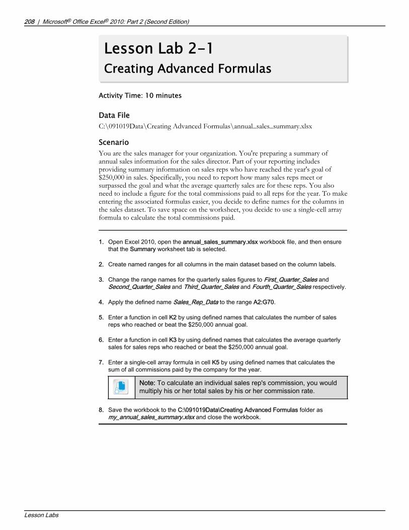
Lesson Lab 2-1Creating Advanced Formulas

Activity Time: 10 minutes

Data FileC:\091019Data\Creating Advanced Formulas\annual_sales_summary.xlsx

ScenarioYou are the sales manager for your organization. You're preparing a summary ofannual sales information for the sales director. Part of your reporting includesproviding summary information on sales reps who have reached the year's goal of$250,000 in sales. Specifically, you need to report how many sales reps meet orsurpassed the goal and what the average quarterly sales are for these reps. You alsoneed to include a figure for the total commissions paid to all reps for the year. To makeentering the associated formulas easier, you decide to define names for the columns inthe sales dataset. To save space on the worksheet, you decide to use a single-cell arrayformula to calculate the total commissions paid.

1. Open Excel 2010, open the annual_sales_summary.xlsx workbook file, and then ensurethat the Summary worksheet tab is selected.

2. Create named ranges for all columns in the main dataset based on the column labels.

3. Change the range names for the quarterly sales figures to First_Quarter_Sales andSecond_Quarter_Sales and Third_Quarter_Sales and Fourth_Quarter_Sales respectively.

4. Apply the defined name Sales_Rep_Data to the range A2:G70.

5. Enter a function in cell K2 by using defined names that calculates the number of salesreps who reached or beat the $250,000 annual goal.

6. Enter a function in cell K3 by using defined names that calculates the average quarterlysales for sales reps who reached or beat the $250,000 annual goal.

7. Enter a single-cell array formula in cell K5 by using defined names that calculates thesum of all commissions paid by the company for the year.

Note: To calculate an individual sales rep's commission, you wouldmultiply his or her total sales by his or her commission rate.

8. Save the workbook to the C:\091019Data\Creating Advanced Formulas folder asmy_annual_sales_summary.xlsx and close the workbook.


Lesson Labs

Do Not D

uplicate

or Dist

ribute

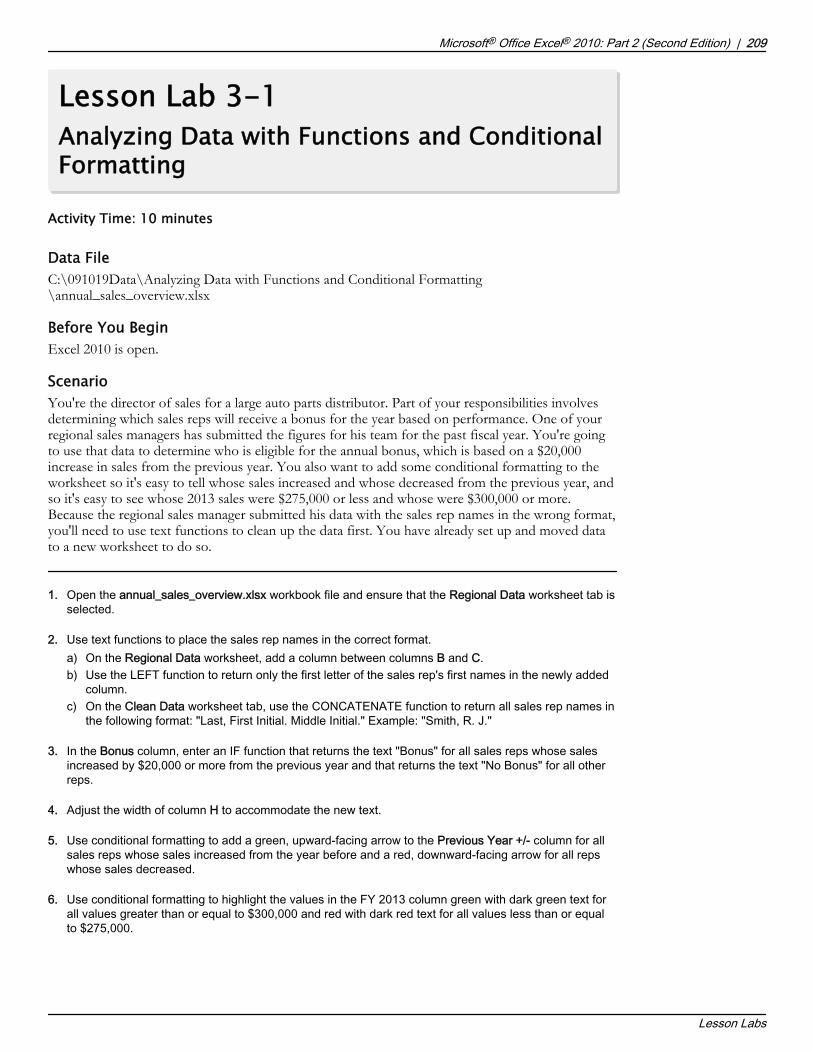
Lesson Lab 3-1Analyzing Data with Functions and ConditionalFormatting


Data FileC:\091019Data\Analyzing Data with Functions and Conditional Formatting\annual_sales_overview.xlsx


ScenarioYou're the director of sales for a large auto parts distributor. Part of your responsibilities involvesdetermining which sales reps will receive a bonus for the year based on performance. One of yourregional sales managers has submitted the figures for his team for the past fiscal year. You're goingto use that data to determine who is eligible for the annual bonus, which is based on a $20,000increase in sales from the previous year. You also want to add some conditional formatting to theworksheet so it's easy to tell whose sales increased and whose decreased from the previous year, andso it's easy to see whose 2013 sales were $275,000 or less and whose were $300,000 or more.Because the regional sales manager submitted his data with the sales rep names in the wrong format,you'll need to use text functions to clean up the data first. You have already set up and moved datato a new worksheet to do so.

1. Open the annual_sales_overview.xlsx workbook file and ensure that the Regional Data worksheet tab isselected.

2. Use text functions to place the sales rep names in the correct format.a) On the Regional Data worksheet, add a column between columns B and C.b) Use the LEFT function to return only the first letter of the sales rep's first names in the newly added

column.c) On the Clean Data worksheet tab, use the CONCATENATE function to return all sales rep names in

the following format: "Last, First Initial. Middle Initial." Example: "Smith, R. J."

3. In the Bonus column, enter an IF function that returns the text "Bonus" for all sales reps whose salesincreased by $20,000 or more from the previous year and that returns the text "No Bonus" for all otherreps.

4. Adjust the width of column H to accommodate the new text.

5. Use conditional formatting to add a green, upward-facing arrow to the Previous Year +/- column for allsales reps whose sales increased from the year before and a red, downward-facing arrow for all repswhose sales decreased.

6. Use conditional formatting to highlight the values in the FY 2013 column green with dark green text forall values greater than or equal to $300,000 and red with dark red text for all values less than or equalto $275,000.


Lesson Labs

Do Not D

uplicate

or Dist

ribute

7. Save the workbook to the C:\091019Data\Analyzing Data with Functions and ConditionalFormatting folder as my_annual_sales_overview.xlsx and then close the workbook.


Lesson Labs

Do Not D

uplicate

or Dist

ribute

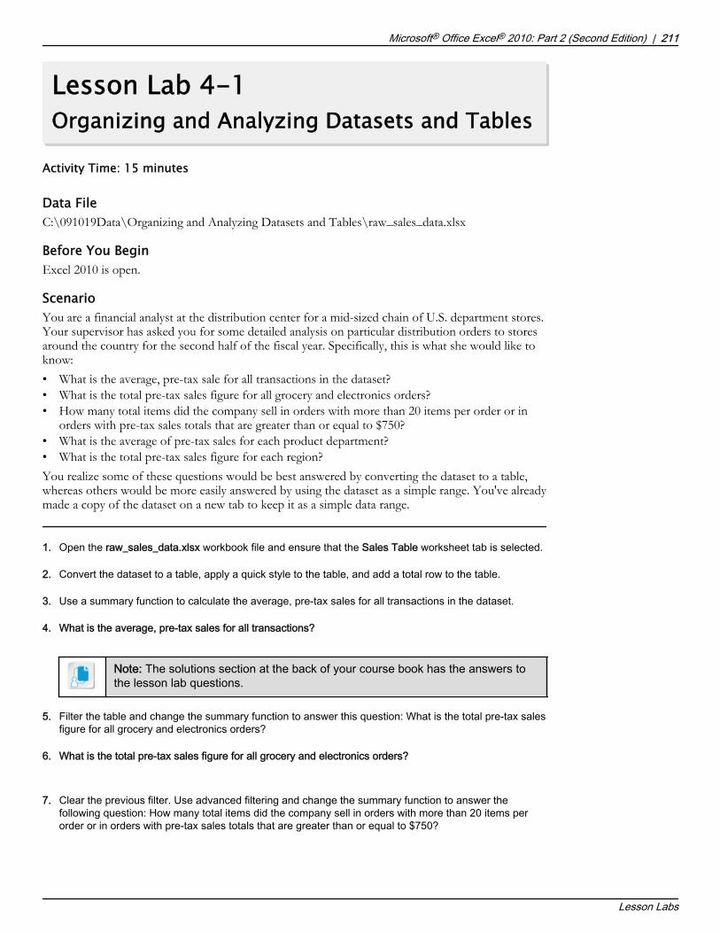
Lesson Lab 4-1Organizing and Analyzing Datasets and Tables


Data FileC:\091019Data\Organizing and Analyzing Datasets and Tables\raw_sales_data.xlsx


ScenarioYou are a financial analyst at the distribution center for a mid-sized chain of U.S. department stores.Your supervisor has asked you for some detailed analysis on particular distribution orders to storesaround the country for the second half of the fiscal year. Specifically, this is what she would like toknow:• What is the average, pre-tax sale for all transactions in the dataset?• What is the total pre-tax sales figure for all grocery and electronics orders?• How many total items did the company sell in orders with more than 20 items per order or in

orders with pre-tax sales totals that are greater than or equal to $750?• What is the average of pre-tax sales for each product department?• What is the total pre-tax sales figure for each region?You realize some of these questions would be best answered by converting the dataset to a table,whereas others would be more easily answered by using the dataset as a simple range. You've alreadymade a copy of the dataset on a new tab to keep it as a simple data range.

1. Open the raw_sales_data.xlsx workbook file and ensure that the Sales Table worksheet tab is selected.

2. Convert the dataset to a table, apply a quick style to the table, and add a total row to the table.

3. Use a summary function to calculate the average, pre-tax sales for all transactions in the dataset.

4. What is the average, pre-tax sales for all transactions?A: $526.99

Note: The solutions section at the back of your course book has the answers tothe lesson lab questions.

5. Filter the table and change the summary function to answer this question: What is the total pre-tax salesfigure for all grocery and electronics orders?

6. What is the total pre-tax sales figure for all grocery and electronics orders?A: $36,575.83

7. Clear the previous filter. Use advanced filtering and change the summary function to answer thefollowing question: How many total items did the company sell in orders with more than 20 items perorder or in orders with pre-tax sales totals that are greater than or equal to $750?


Lesson Labs

Do Not D

uplicate

or Dist

ribute

8. How many total items did the company sell in orders with more than 20 items per order orin orders with pre-tax sales totals that are greater than or equal to $750?A: 3,255

9. Switch to the Sales Range worksheet and use the Subtotals feature to answer thefollowing question: What is the average of pre-tax sales for each product department?

10. What is the average of pre-tax sales for each product department?A: Athletics: $64.93; Auto: $547.62; Clothing: $523.14; Electronics: $530.49; Grocery:

$486.72; Health/Beauty: $514.74; Housewares: $515.63; and Toys: $541.03.

11. Re-sort the dataset and then use the Subtotals feature to answer the following question:What is the total pre-tax sales figure for each region?

12. What is the total pre-tax sales figure for each region?A: MW: $33,115.11; NE: $31,003.65; SE: $32,033.91; SW: $28,644.77; and West:

$32,773.09.

13. Save the workbook to the C:\091019Data\Organizing and Analyzing Datasets and Tablesfolder as my_raw_sales_data.xlsx and close the workbook.


Lesson Labs

Do Not D

uplicate

or Dist

ribute

Lesson Lab 5-1Visualizing Data with Basic Charts


Data FileC:\091019Data\Visualizing Data with Basic Charts\top_sellers.xlsx


ScenarioYou have just finished summarizing sales figures for your team for the past year. You have created asummary dataset for your five top-selling sales reps. You want to report on their success at anupcoming meeting and you feel that using a chart would be the best way to do so. You plan to add a3-D column chart to the worksheet and modify it a bit to make it easier to interpret.

1. Open the top_sellers.xlsx workbook file and ensure that the Summary worksheet tab is selected.

2. Add a 3-D Clustered Column chart to the worksheet based on the quarterly sales data for the salesreps. Do not include the Total column or the Grand Total figure in the chart.

3. Position the chart directly to the right of the original dataset near the very top of the worksheet.

4. Resize the chart so that it takes up most of the visible space to the right of the dataset.

5. Apply the Style 42 chart quick style to the chart.

6. Add a title to the chart title at the top of the chart that reads Top Sellers

7. Add an X-axis title below the chart that reads Sales Reps and add a vertical title for the Y axis thatreads Quarterly Sales

8. Save the workbook to the C:\091019Data\Visualizing Data with Basic Charts folder asmy_top_sellers.xlsx and then close the workbook.


Lesson Labs

Do Not D

uplicate

or Dist

ribute

Lesson Lab 6-1Analyzing Data with PivotTables andSlicers


Data FileC:\091019Data\Analyzing Data with PivotTables, Slicers, and PivotCharts\raw_sales_data2.xlsx


ScenarioYou've been asked to analyze your company's sales for the first month of the fiscalyear. You supervisor has asked you several questions about your sales data and expectsyou to report back with your findings before the end of the day. As you will need toanalyze the raw data from a number of different perspectives in a short period of time,you decide to create a PivotTable out of the raw data and to add slicers for the keyfields you will analyze. These are the questions from your supervisor:• How many of each item was sold from the housewares department for the month?• What department sold the most number of items for the month, and what

percentage of overall items sold does that represent?• Which region has the highest pre-tax toy sales for the month and what was the sales

total?• Which three markets had the highest pre-tax sales in the electronics department and

what are the sales totals?• Which market has the highest average of clothing items sold per sale and how many

items does it average?

1. Open the raw_sales_data2.xlsx workbook file and ensure that the Jan Sales Dataworksheet tab is selected.

2. Create a PivotTable out of the entire dataset that appears on the same worksheet as thedata.

3. Insert slicers for the Region, Department, and Item Number columns.

4. Use the PivotTable to answer this question: How many of each item did the company sellfrom the housewares department for the month?

5. How many of each item did the company sell from the housewares department for themonth?A: Item 7001: 205; item 7002: 108; item 7003: 223; item 7004: 198; and item 7005:

102.

6. Use the PivotTable to answer the following question: What department sold the mostnumber of items for the month and what percentage of overall items sold does thatrepresent?


Lesson Labs

Do Not D

uplicate

or Dist

ribute

7. What department sold the most number of items for the month and what percentage of overall itemssold does that represent?A: Housewares: 14.3 percent

8. Use the PivotTable to answer the following question: Which region has the highest pre-tax toy sales forthe month and what was the sales total?

9. Which region has the highest pre-tax toy sales for the month and what was the sales total?A: The Midwest (MW) region with $4,940.81 in toy sales.

10. Use the PivotTable to answer this question: Which three markets had the highest pre-tax sales in theelectronics department and what are the sales totals?

11. Which three markets had the highest pre-tax sales in the electronics department and what are the salestotals?A: Midwest (MW): $4,834.58; Southwest (SW): $4,183.65; and West: $3,265.67.

12. Use the PivotTable to answer this question: Which market has the highest average of clothing itemssold per sale and how many items does it average?

13. Which market has the highest average of clothing items sold per sale and how many items does itaverage?A: The Northeast (NE) region with an average of 21.14 clothing items sold per sale.

14. Save the workbook to the C:\091019Data\Analyzing Data with PivotTables, Slicers, and PivotChartsfolder as my_raw_sales_data2.xlsx close the workbook and close Excel 2010.


Lesson Labs

Do Not D

uplicate

or Dist

ribute

Do Not D

uplicate

or Dist

ribute

Solutions

ACTIVITY 2-3: Locating and Using Specialized Functions

2. Which of these functions would best answer the question: How many authors have been withthe company for five or fewer years?A: COUNTIF

ACTIVITY 4-3: Filtering Data

2. How many titles sell at the highest price?A: 43

6. Does the COUNT function result in the Sell Price column answer the question "How manyauthors have been with the company for one year or less?"A: Yes, the COUNT function in any of the total row cells would give the correct answer. A totalof 48 authors have been with the company one year or less.Let the students know that the built-in functions in the Total row of tables reflect the currentlyfiltered state of the table. So, in this case, for any filter performed, the COUNT function wouldaccurately count the unfiltered entries.

ACTIVITY 4-5: Using Summary Functions in Tables

5. How many authors signed their initial contracts in 2012?A: 64

6. How much income did those authors produce?A: $197,351,621.43

Do Not D

uplicate

or Dist

ribute

ACTIVITY 4-6: Using Database Functions

3. What is the average number of books sold for these authors?A: 427,179

5. What is the total income earned by these authors?A: $550,441,558

LAB 4-1: Organizing and Analyzing Datasets andTables

4. What is the average, pre-tax sales for all transactions?A: $526.99The solutions section at the back of your course book has the answers to the lesson labquestions.

6. What is the total pre-tax sales figure for all grocery and electronics orders?A: $36,575.83

8. How many total items did the company sell in orders with more than 20 items per order orin orders with pre-tax sales totals that are greater than or equal to $750?A: 3,255

10. What is the average of pre-tax sales for each product department?A: Athletics: $64.93; Auto: $547.62; Clothing: $523.14; Electronics: $530.49; Grocery:$486.72; Health/Beauty: $514.74; Housewares: $515.63; and Toys: $541.03.

12. What is the total pre-tax sales figure for each region?A: MW: $33,115.11; NE: $31,003.65; SE: $32,033.91; SW: $28,644.77; and West:$32,773.09.

ACTIVITY 6-2: Analyzing PivotTable Data

4. Which genre is the biggest overall seller?A: Romance with 110,272,958 copies sold

6. What is the total number of units of fantasy and romance books sold in the APAC andEMEA markets?A: 64,309,243

8. What percentage of total sales is made up of fantasy sales in the LA market?A: 2.91 percent

10. Which market has the highest percentage of science fiction sales?A: The NA market with 26.84 percent.


Solutions

Do Not D

uplicate

or Dist

ribute

14. Which author has the lowest total sales?A: Author 1017 with $5,454,183.55

16. Which book for author 1017 has generated the most sales?A: BookTitle0135 with $2,390,754.44 in sales

18. What percentage of author 1048's total sales are electronic book sales?A: 15.21 percent

ACTIVITY 6-3: Presenting Data with PivotCharts

3. Which genre/market pair is the most successful in terms of number of units sold?A: The romance genre in the NA market.

ACTIVITY 6-4: Filtering Data by Using Slicers

5. How many romance print books has author 1029 sold in the APAC market?A: 1,935,355

8. Of author 1056's electronic fantasy and science fiction book sales in the NA market, what percentage isrepresented by science fiction sales?A: 31.42 percent

LAB 6-1: Analyzing Data with PivotTables and Slicers

5. How many of each item did the company sell from the housewares department for the month?A: Item 7001: 205; item 7002: 108; item 7003: 223; item 7004: 198; and item 7005: 102.

7. What department sold the most number of items for the month and what percentage of overall itemssold does that represent?A: Housewares: 14.3 percent

9. Which region has the highest pre-tax toy sales for the month and what was the sales total?A: The Midwest (MW) region with $4,940.81 in toy sales.

11. Which three markets had the highest pre-tax sales in the electronics department and what are the salestotals?A: Midwest (MW): $4,834.58; Southwest (SW): $4,183.65; and West: $3,265.67.

13. Which market has the highest average of clothing items sold per sale and how many items does itaverage?A: The Northeast (NE) region with an average of 21.14 clothing items sold per sale.


Solutions

Do Not D

uplicate

or Dist

ribute

Do Not D

uplicate

or Dist

ribute

Glossary

add-insSupplemental programs for MicrosoftOffice applications that provide additionalfeatures and functionality not available in astandard installation.

arrayA range of data that can be entered into acomputer's memory and accessed by Excelfor data analysis that does not necessarilyhave to exist within worksheet cells.

array constantsSeries of values, logical values, or textentries that are stored in memory orentered directly into array formulas, asopposed to being entered in cells.

array formulasType of Excel formula that allows users toperform multiple calculations on cells in anarray simultaneously.

AutoFiltersPreconfigured, common filtering optionsthat enable Excel users to quickly removefrom view all data that does not meet somespecified criteria.

cell namesMeaningful names users can assign toparticular cells to make it easier to bothunderstand what specific calculations arebeing performed in a formula and reusethe references for a number of purposes.

chart elementsThe individual objects that can appear oncharts and that convey some level ofinformation to a viewer about the chart'sdata.

chartsGraphical representations of the numericvalues and relationships in a dataset.

color scalesVarious shades of color used as graphicalrepresentation of the relative values of celldata. Color scales are a type of conditionalformatting.

comparison operatorsAnother term for logical operators.

criteria rangeIn terms of Excel advanced filtering anddatabase functions, the worksheet rangethat contains the user-defined criteria toperform a particular operation.

Ctrl+Shift+Enter formulasAlso known as CSE formulas. Alternatename for Excel array formulas, as usersmust press Ctrl+Shift+Enter to enter anarray formula.

custom AutoFiltersUser-defined Excel AutoFilters.

custom sortA user-defined sort that can be applied toeither rows or columns, can be applied to

Do Not D

uplicate

or Dist

ribute

multiple rows or columns simultaneously,and that can be highly customized.

data barsGraphical representations of the relativevalue of data in a range of cells comparedto the rest of the data in the same range.Data bars are a type of conditionalformatting.

database functionsSet of Excel functions that enable users toperform calculations on ranges of databased on specific criteria.

entryAn individual row of data in a transactionaldataset. An entry represents one singletransaction, such as a sale.

fieldsThe columns in a transactional dataset.

filteringThe process of removing from view anydata entries that do not match somespecified criteria.

icon setsCollections of images used as graphicalrepresentations of the relative values of celldata. Icon sets are a type of conditionalformatting.

levelIn terms of Excel custom sorting, anindependent, specific criterion by which adataset is sorted. Users can specify multiplelevels for a custom sort.

logical operatorsType of Excel operator used to compareparticular values to determine whether ornot they meet some specified criteria.

logical valuesExcel data type that expresses whether ornot particular data meets some specifiedcriteria. There are only two logical values inExcel, TRUE and FALSE.

multi-cell array formulaArray formula that performs multiplecalculations on arrays and display theresults in multiple cells.

outlineExcel feature that enables users to organizedatasets into hierarchical groups of varyinglevels of detail that they can expand orcollapse depending on how much detailthey want to see.

PivotChartsSimilar to standard Excel charts, these aregraphical representations of numeric valuesand relationships among those values. Thekey difference between charts andPivotCharts is that PivotCharts are linkedto the data in PivotTables.

pivotingIn Excel, a form of data manipulation thatcan take a column of data and pivot it intoa row and vice versa.

PivotTableA dynamic Excel data object that enablesusers to perform data analysis by pivotingcolumns and rows of raw data withoutaltering the raw data.

quick sortsPreconfigured sorting options that enableworkbook users to quickly sort data basedon common criteria.

quick stylesPreconfigured table styles.

range namesMeaningful names users can assign toparticular ranges to make it easier to bothunderstand what specific calculations arebeing performed in a formula and reusethe references for a number of purposes.

rule precedenceThe order in which Excel evaluates andapplies conditional formatting rules tocells.


Glossary

Do Not D

uplicate

or Dist

ribute

separatorsVertical boundaries users can insert intothe Quick Access Toolbar to organizecommands into related groups.

shared slicersSlicers that are connected to and that filtermultiple PivotTables simultaneously. AnyPivotTables based on a common dataset canshare slicers.

single-cell array formulaArray formula that performs multiplecalculations on arrays and display the result in asingle cell.

slicersIndividual Excel objects used to filter the datain PivotTables.

sortingThe process of reordering worksheet databased on some defined criteria, such asalphabetically or from highest value to lowestvalue.

SUBTOTAL functionsA specific set of Excel functions that performcalculations on subsets of data.

subtotals featureExcel feature that enables users toautomatically perform SUBTOTAL functioncalculations on subsets of data within aparticular dataset.

summary functionsExcel feature that automatically performsSUBTOTAL function calculations in tables.Users can access this functionality from thetotal row down arrows in each column.

tableA dataset comprised of contiguous rows andcolumns that Excel treats as a single,independent object.

table stylesParticular configurations of formatting optionsusers can apply to worksheet tables.

text paneElement of the Excel user interface thatenables users to add and edit text on SmartArtgraphics.

transactional dataData that represents each individualtransaction, or event, in a series of transactions,and that is not summarized in any way shapeor form. Transactional data does not typicallycontain row labels, only column labels.


Glossary

Do Not D

uplicate

or Dist

ribute

Do Not D

uplicate

or Dist

ribute

Index

Aadd-ins 18, 19AND function 60array formulas 43arrays

constants 46defined 43formula syntax 46

AutoCorrect feature 4, 5AutoFilters 96, 97AVERAGEIF function 37

Ccell names

defined 24entering manually 30in formulas 30Name Manager dialog box 27New Name dialog box 25, 26Use in Formula command 30

chart elements 129charts 122–125Chart Tools contextual tab 130, 131color scales 69comparison operators 59CONCATENATE function 56conditional formats 71Conditional Formatting Rules Managerdialog box 73, 74COUNTA function 39COUNTIF function 38Create from Selection command 26Create Table dialog box 82criteria range 99

CSE formulas 44Ctrl-Shift-Enter formulas, See CSEformulasCustom AutoFilter dialog box 97, 98Customize Ribbon tab 10, 11custom sorts 89

Ddata bars 68database functions 115, 116

Eentry 140

Ffields 140filtering 95, 98filter operators 100formatting 128Formula AutoComplete feature 31formulas

cell names 30multi-cell array 44options 3range names 30single-cell array 45

function categories 34functions

AND 60AVERAGEIF 37CONCATENATE 56COUNTA 39COUNTIF 38

Do Not D

uplicate

or Dist

ribute

IF 61IFS 38LEFT 54LEN 55LOWER 56MID 55OR 60PMT 39PROPER 56STDEV.P 39SUMIF 37syntax 37TRIM 55UPPER 56

Iicon sets 70IF function 61IFS functions 38interface, customizing 3

Llanguage options 5LEFT function 54LEN function 55levels 89logical

functions 58operators 36, 59values 58

LOWER function 56

MMID function 55modification 128multi-cell array formulas 44

NName Box 25Name Manager dialog box 27New Formatting Rule dialog box 71, 72New Table Quick Style dialog box 83

OOR function 60outlines 109

PPivotCharts 157, 158pivoting 138PivotTables 139, 141, 146, 148, 149PMT function 39proofing options 4PROPER function 56

QQuick Access Toolbar 3, 12–14quick sorts 89quick styles 82

Rrange names

defined 24entering manually 30in formulas 30Name Box 25Name Manager dialog box 27New Name dialog box 25, 26Use in Formula command 30

ribbon customization 10–12rule precedence 74

Ssaving options 5Select Data Source dialog box 131separators 12shared slicers 164single-cell array formulas 45slicers 162–164Sort dialog box 90sorting 87–89Sort Options dialog box 90STDEV.P function 39SUBTOTAL functions 105, 106, 108, 109Subtotals feature 107SUMIF function 37summary functions 110syntax

array formulas 46database functions 116

Ttables

components 81defined 80


Index

Do Not D

uplicate

or Dist

ribute

table styles 82Table Tools contextual tab 82text functions 54transactional data 140TRIM function 55Trust Center 3, 6, 7

UUPPER function 56Use in Formula command 30


Index

Do Not D

uplicate

or Dist

ribute

Do Not D

uplicate

or Dist

ribute

091019S rev 1.0Do Not D

uplicate

or Dist

ribute