Distinguishing Limited Liability from Moral Hazard in a Model of Entrepreneurship∗ Anna L. Paulson, Robert Townsend and Alexander Karaivanov

Fe

dera

l Res

erve

Ban

k of

Chi

cago

REVISED April, 2005 WP 2003-06

Distinguishing Limited Liability from Moral Hazard in a Model

of Entrepreneurship∗

Anna L. PaulsonFederal Reserve Bank of Chicago

Robert TownsendUniversity of Chicago

Federal Reserve Bank of Chicago

Alexander KaraivanovSimon Fraser University

April, 2005

Abstract

We present and estimate a model where the choice between entrepreneurship and wagework may be influenced by financial market imperfections. The model allows for limitedliability, as in Evans and Jovanovic (1989), moral hazard, as in Aghion and Bolton (1996),and a combination of both constraints. The paper uses structural techniques to estimatethe model and identify the source of financial market imperfections using data fromrural and semi-urban households in Thailand. Structural, non-parametric and reducedform estimates provide independent evidence that the dominant source of credit marketimperfections is moral hazard. We reject the hypothesis that limited liability alone canexplain the data.

∗A previous version of this paper has been circulated under the title ”Distinguishing LimitedCommitment from Moral Hazard in Models of Growth with Inequality.” That version is availableat: http://www.chicagofed.org/publications/workingpapers/papers/wp2003-06.pdf. Comments from DaronAcemoglu, Patrick Bolton, Lars Hansen, Boyan Jovanovic, Andreas Lehnert, Bernard Salanie, Chris Udry,two anonymous referees, the editor of this journal and from conference and seminar participants at the Fed-eral Reserve Bank of Chicago, DELTA, IUPUI, MIT, UCLA, the University of Toulouse, Stanford and Yaleare gratefully acknowledged. We also thank Francisco Buera, Xavier Gine and Yukio Koriyama for excellentresearch assistance as well as the National Institute of Health and the National Science Foundation for fund-ing. We are much indebted to Sombat Sakuntasathien for collaboration and for making the data collectionpossible. The views expressed in this paper are those of the authors and do not necessarily represent those ofthe Federal Reserve Bank of Chicago or the Federal Reserve System.

1

1 Introduction

Financial market imperfections shape economic outcomes in many areas. In studying theseoutcomes, many papers posit a particular financial market imperfection and exclude thepossibility of alternative sources of imperfections. The goal of this paper is to identify thesource of financial constraints that limit entry into entrepreneurship. We use structural,non-parametric and reduced form techniques to distinguish the source of financial marketimperfections using microeconomic data from Thailand.

Earlier work demonstrates that financial constraints have an important effect on whostarts businesses and on how existing businesses are run in Thailand (see Paulson andTownsend, 2004). A symptom of financial constraints is that wealth will be positively cor-related with the probability of starting a business, holding constant the characteristics ofpotential entrepreneurs. A strong positive correlation between becoming an entrepreneurand beginning-of-period wealth can be seen in the non-parametric regression displayed inFigure 1.1 However, a positive correlation between wealth and entrepreneurship only demon-strates that financial constraints are likely to be important but does not illuminate the sourceof the constraint.

The literature identifies two main sources of financial constraints that influence the deci-sion to become an entrepreneur. In Evans and Jovanovic (1989), the financial constraint isdue to limited liability. Agents can supplement their personal stake in entrepreneurial activi-ties by borrowing. Wealth plays the role of collateral and limits default. In this environmentlow-wealth households may be prevented from borrowing enough to become entrepreneursand others, who are able to start businesses, may be constrained in investment. Limitedliability is also featured in a variety of empirical studies of occupational choice. Evans andJovanovic (1989) and Magnac and Robin (1996) provide structural estimates of this modelfor the U.S. and for France, respectively. In a limited liability environment, constrained en-trepreneurs borrow more when wealth increases. With limited liability, borrowing does notautomatically imply being constrained. Some entrepreneurs may be able to borrow enoughto invest the optimal amount of capital, as though there were no constraints

Financial constraints that arise from moral hazard are the focus of the model of occupa-tional choice featured in Aghion and Bolton (1996). Since entrepreneurial effort is unobservedand repayment is only feasible if a project is successful, poor borrowers have little incentiveto be diligent, increasing the likelihood of project failure and default. In order to break-even,lenders charge higher interest rates to low-wealth borrowers. Some low-wealth potential en-trepreneurs will be unable, or unwilling at such high interest rates, to start businesses at anyscale. Low-wealth entrepreneurs who do succeed in getting loans will be subject to a bindingincentive compatibility constraint that ensures that they exert the appropriate level of effort.In contrast to the limited liability case, when there is moral hazard and wealth increases,constrained entrepreneurs will increasingly self-finance and borrowing diminishes. In a moralhazard environment, all entrepreneurs who borrow will be constrained2.

The model that we estimate takes into account entrepreneurial talent, allows investment

1For each observation in Figure 1, a weighted regression is performed using 80% (bandwidth = 0.8) of thedata around that point. The data are weighted using a tri-cube weighting procedure that puts more weighton the points closest to the observation in question. The weighted regression results are used to produce apredicted value for each observation. Because the graphs can be fairly sensitive to outliers, we have droppedthe wealthiest 1% of the sample.

2This is true if the moral hazard enviroment does not produce the same solution as the first best which isgenerally the case.

2

to be divisible and agents to be risk averse. Because the scale of the business can vary, therelationship between wealth and borrowing is not driven by indivisibilities. In addition, themodel allows entrepreneurial talent to depend on wealth and formal education. Regardlessof the assumptions regarding financial constraints, the model implies that entrepreneurshipwill be positively related to pre-existing wealth. Of course the specific functional relationshipbetween entrepreneurship and wealth will depend on the financial constraint. In addition,as discussed above, the relationship between being a borrower and being constrained andthe response of constrained entrepreneurs to an increase in wealth depends on the financialmarket imperfection. In particular, if limited liability constraints financial markets, increasesin wealth will allow constrained entrepreneurs to borrow more. However, not all borrowersneed be constrained when there is limited liability. If moral hazard is the source of con-straints, increases in wealth will be associated with less borrowing, and all borrowers will beconstrained.

A central goal of this paper is to see if limited liability can be distinguished from moralhazard in structural estimates using cross-sectional data from a sample of households fromThailand. We also consider the possibility that both are important.3 The estimated mod-els share a common technology, as well as common preferences and assumptions about thedistribution of talent. They differ only in the assumed financial constraint. The appropri-ate Vuong (1989) test is used to compare the structural estimates and to determine whichsingle financial constraint is most consistent with the data on entrepreneurial status, initialwealth and education; or if both are important. The Vuong test is also featured in Wolak(1994) and Fafchamps (1993). The structural model comparison tests are augmented withnon-parametric and reduced form estimates that capitalize on the richness of the data, whichinclude information on household characteristics, borrowing, and collateral.

This paper is related to other work that tries to identify the underlying source of marketimperfections. For example, Abbring, Chiappori, Heckman and Pinquet (2002) use dynamicdata to distinguish moral hazard from adverse selection in the insurance context. Their worktakes the insurance contract as given, based on the regulatory environment. Our treatment ofthe limited liability constraint is conceptually similar. We assume a standard debt contractand estimate the parameter that determines how much a potential entrepreneur can borrowas a function of wealth and entrepreneurial talent. The estimation is more innovative whenthe financial environment is affected by moral hazard. The estimated financial contractis the endogenous solution to the mechanism design problem that satisfies the incentivecompatibility constraint. To our knowledge, this is the first paper to provide structuralestimates of a moral hazard model of occupational choice based on a mechanism designapproach.

The Thai data come from a socioeconomic survey that was fielded in March - May of 1997to 2,880 households, approximately 21% of whom run their own businesses.4 The samplefocuses on households living in two distinct regions of the country: rural and semi-urbanhouseholds living in the central region, close to Bangkok, and more obviously rural householdsliving in the semi arid and much poorer northeastern region.5 The data include current

3We have also considered the possibility that occupation choices are first best and that there is neitherlimited liability nor moral hazard. Structural, reduced form and non-parametric findings reject this possibility.

4For esimation purposes, the data are restricted to households who have non-zero wealth and who eithercurrently own a business that was founded in the five years prior to the survey (14%) or who have no businessat the time of the survey (86%).

5See Binford, Lee and Townsend (2001) for more details on the sampling methodology.

3

and retrospective information on wealth (household, agricultural, business and financial),occupational history (transitions to and from farm work, wage work and entrepreneurship),as well as access and use of a wide variety of formal and informal financial institutions(commercial banks, agricultural banks, village lending institutions, money lenders, as wellas friends, family and business associates). The data also provide detailed information onhousehold demographics, education and entrepreneurial activities.

The results indicate that progress can be made in identifying the nature of financialconstraints. The dominant source of constraints is moral hazard. We reject the hypothesisthat limited liability alone can explain the data. The evidence in favor of moral hazard isparticularly strong for the wealthier Central region. For the poorer Northeastern region, wecannot rule out that limited liability may have a role to play, but only in combination withmoral hazard.

These conclusions are based both on the formal financial regime comparison tests from thestructural estimation, which use data on wealth, education and entrepreneurial status, as wellas on reduced form and non-parametric estimates, which use data on wealth, entrepreneurialstatus, net savings, as well as other important household characteristics. The formal financialregime comparison tests are necessarily only informative about the relative success of a givenfinancial regime for the particular set of assumptions regarding preferences, technology etc.that are imposed by the model. In contrast, the reduced form and non-parametric estimatesexamine implications that are likely to distinguish moral hazard from limited liability for alarge class of potential assumptions.

The rest of the paper is organized as follows. In the next section, the model and thefinancial constraints are presented. Section three describes the computational algorithm forthe structural maximum likelihood estimation. Section four describes the data. Sectionfive reports on the structural maximum likelihood parameter estimates. In section six, wedetermine which financial regime best fits the data using structural, reduced form and non-parametric techniques. The final section concludes and suggests directions for future research.

2 Model and Implications

In this section, we describe the model of occupational choice and provide intuition for thesolutions and the relationships among key variables. Since structural estimation lends itselfto characterizing the model in a different, but equivalent way, this section also describes thegeneral linear programming problem that forms the basis of the structural estimation. Thebasic structure of the model — preferences, endowments and technology — is the same regard-less of the financial environment. The financial environment depends on which constraintsare assumed to bind: limited liability, moral hazard or both.

2.1 Economic Environment

Households are assumed to derive utility, U , from their own consumption, c, and disutilityfrom effort, z:

U(c, z) =c1−γ11− γ1

− κzγ2

γ2(1)

We assume that utility displays constant relative risk aversion in consumption. The parameterγ1 ≥ 0 determines the degree of risk aversion. The parameters κ > 0 and γ2 ≥ 1 determinethe loss in utility from expending effort. Consumption, c, and effort, z, must be non-negative.

4

In discussing the implications of the model, we begin by assuming that agents are risk neu-tral, in other words that γ1 is equal to zero. We reintroduce risk aversion in the presentationof the linear programming problem that forms the basis for the structural estimation.

There are three sources of household heterogeneity in the model: initial wealth, A, en-trepreneurial talent, θ, and years of education, S. All of these variables are determined exante and can be observed by all of the agents in the model.6 Wealth is assumed to lie in theinterval (0, 1]. We assume talent is log normally distributed. Specifically:

ln θ = δ0 + δ1 ln (A) + δ2 ln(1 + S) + η, (2)

where η is normally distributed with mean zero and variance ση. In order to avoid thespurious inference that wealth rather than talent is the source of constraints, an individual’sexpected talent can be correlated with wealth through δ1. Talent may also be correlated withformal education via δ2.

Entrepreneurs produce output q from their own effort z and from capital k. Output qcan take on two values, namely q = θ, which corresponds to success and occurs with positiveprobability, and q = 0, which is equivalent to bankruptcy and occurs with the remainingprobability. Note that output is increasing in entrepreneurial talent, θ. The technology isstochastic and is written P (q = θ|z, k > 0), the probability of achieving output q given effortz, and capital k. Specifically:7

P (q = θ|z, k > 0) =kαz1−α

1 + kαz1−α(3)

Output can be costlessly observed by everyone.When k = 0, the firm is not capitalized. This means that the household works in the

wage sector. Earnings, w, in the wage sector are also stochastic and depend on effort. Theyare equal to one with probability z

1+z and equal to zero with the residual probability.8

All households are price-takers and take the gross cost of borrowing, r(A, θ), which mayvary with wealth and entrepreneurial talent, as given. Entrepreneurs who do not borrow(who have k < A) and wage workers earn the given, riskless gross interest rate, r, on theirnet savings.

Occupational assignments are determined by a social planner who maximizes agents’utility subject to constraints that describe the financial intermediary and any financial marketimperfections. This approach is equivalent to a situation in which a large number of financialinstitutions compete to attract clients so that in the end it is as if the agents in the economymaximize their utility subject to the financial institution earning zero profits, and subject,of course, to constraints having to do with financial market imperfections.

In sum, when agents are risk neutral, the planner makes an effort recommendation, z,and a capital recommendation, k to solve:

Maxz,k

w z1+z − κzγ2

γ2+ rA, if k = 0

θ kαz1−α1+kαz1−α − κzγ2

γ2+ r(A− k), if k > 0, k ≤ A

θ kαz1−α1+kαz1−α − κzγ2

γ2− r(A, θ)(k −A) kαz1−α

1+kαz1−α , if k > 0, k > A

(4)

6The complications in estimation that arise from the fact that the econometrician cannot observe θ areaddressed in Section 3.

7The probability of entrepreneurial success is scaled by 1 + kαz1−α to guarantee that it will lie betweenzero and one.

8Again, this formulation guarantees that the probability of success in the wage sector will lie between zeroand one.

5

As one can see above, agents have three possibilities: 1) wage work which corresponds tok = 0; 2) becoming an entrepreneur but not borrowing, which happens when capital ispositive and less than or equal to wealth, k > 0 and k ≤ A; or 3) becoming an entrepreneurand borrowing, which happens when capital is positive and exceeds wealth, k > 0, k > A.

The first term in the maximand is the expected utility of a risk neutral wage worker:expected wages minus the cost of effort, plus a riskless return on wealth. The second term isthe expected utility of a risk neutral entrepreneur who does not need to borrow to carry outthe recommended k: expected output minus the cost of effort, plus a riskless return on anywealth not invested in the project. The final term is the expected utility of an entrepreneurwho must borrow to carry out the assigned k: expected output minus the cost of effort, minusthe expected cost of repaying the loan. Note that the loan is only repaid when the projectis successful. The planner’s problem is subject to a constraint which guarantees that theexpected rate of repayment on such loans covers the cost of outside funds, so that lendersbreak even:

r(A, θ)kαz1−α

1 + kαz1−α= r, for k > A, ∀ θ,∀ A (5)

2.2 Financial Environment

We introduce variations in the financial environment through additional constraints on theplanner’s problem. When financial markets are ”first best” and are subject to neither limitedliability nor moral hazard no further constraints are imposed.

Limited Liability To model limited liability, we assume, as in Evans and Jovanovic (1989),that households can borrow up to some fixed multiple of their total wealth, but no more. Themaximum amount that can be invested in a firm is equal to λA and the maximum amountthat a household can borrow is given by (λ − 1)A. When limited liability is a concern, theplanner’s maximization problem will be subject to:

k ≤ λA (6)

in addition to equation (5).

Moral Hazard When there is moral hazard, entrepreneurial effort is unobservable and thefinancial contract cannot specify an agent’s effort. In terms of the planner’s problem, thistranslates into a requirement that the capital assignment and the interest rate schedule arecompatible with the effort choice that a borrowing entrepreneur would have made on hisor her own. In other words, the capital assignment and the interest rate schedule must notviolate the first order condition with respect to effort of the entrepreneur’s own maximizationproblem. In this case, in addition to equation (5), the planner’s maximization problem willbe subject to:

[θ − r(A, θ)(k −A)]

·(1− α)kαz−α

(1 + kαz1−α)2

¸− κzγ2−1 = 0, (7)

which is an entrepreneurial household’s first order condition for effort, z, for a given interestrate schedule and capital, k.9 Equation (7) requires that the planner’s effort recommenda-tion equate the marginal benefit of effort with the marginal cost of effort plus a term that

9See Karaivanov (2005) for a proof that this approach is valid here.

6

represents the marginal impact of effort on loan repayment, through the effect of effort onthe probability that an entrepreneurial project will be successful: kαz1−α

1+kαz1−α .Note that when agents are risk neutral, moral hazard is only an issue for entrepreneurs who

borrow. The lack of observability of effort is not an issue for wage workers and entrepreneurswho self-finance. The planner can assign effort to them without having to satisfy the incentivecompatibility constraint, equation (7), because there is no moral hazard problem when theoptimal capital investment does not require borrowing.

Moral Hazard and Limited Liability We also consider the possibility that credit mar-kets are characterized by both moral hazard and limited liability. This is modeled by assumingthat the entrepreneurial choice problem is subject to both equation (6) and equation (7), inaddition to equation (5).

2.3 Characterization of Solutions

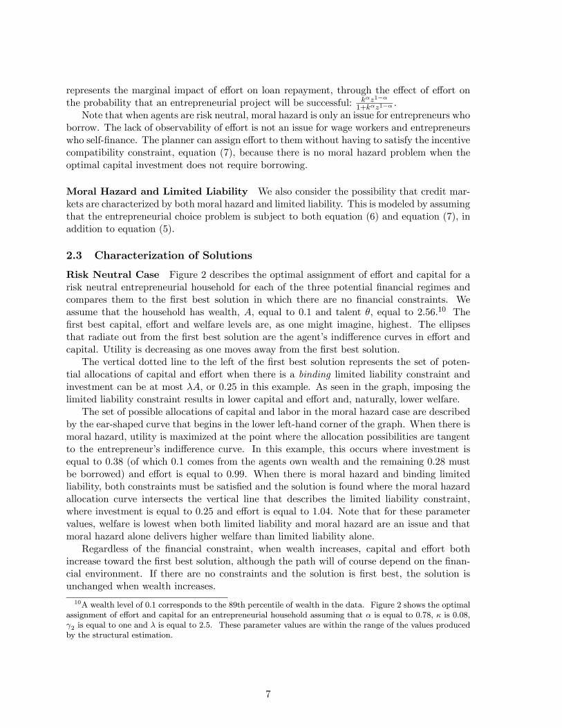
Risk Neutral Case Figure 2 describes the optimal assignment of effort and capital for arisk neutral entrepreneurial household for each of the three potential financial regimes andcompares them to the first best solution in which there are no financial constraints. Weassume that the household has wealth, A, equal to 0.1 and talent θ, equal to 2.56.10 Thefirst best capital, effort and welfare levels are, as one might imagine, highest. The ellipsesthat radiate out from the first best solution are the agent’s indifference curves in effort andcapital. Utility is decreasing as one moves away from the first best solution.

The vertical dotted line to the left of the first best solution represents the set of poten-tial allocations of capital and effort when there is a binding limited liability constraint andinvestment can be at most λA, or 0.25 in this example. As seen in the graph, imposing thelimited liability constraint results in lower capital and effort and, naturally, lower welfare.

The set of possible allocations of capital and labor in the moral hazard case are describedby the ear-shaped curve that begins in the lower left-hand corner of the graph. When there ismoral hazard, utility is maximized at the point where the allocation possibilities are tangentto the entrepreneur’s indifference curve. In this example, this occurs where investment isequal to 0.38 (of which 0.1 comes from the agents own wealth and the remaining 0.28 mustbe borrowed) and effort is equal to 0.99. When there is moral hazard and binding limitedliability, both constraints must be satisfied and the solution is found where the moral hazardallocation curve intersects the vertical line that describes the limited liability constraint,where investment is equal to 0.25 and effort is equal to 1.04. Note that for these parametervalues, welfare is lowest when both limited liability and moral hazard are an issue and thatmoral hazard alone delivers higher welfare than limited liability alone.

Regardless of the financial constraint, when wealth increases, capital and effort bothincrease toward the first best solution, although the path will of course depend on the finan-cial environment. If there are no constraints and the solution is first best, the solution isunchanged when wealth increases.

10A wealth level of 0.1 corresponds to the 89th percentile of wealth in the data. Figure 2 shows the optimalassignment of effort and capital for an entrepreneurial household assuming that α is equal to 0.78, κ is 0.08,γ2 is equal to one and λ is equal to 2.5. These parameter values are within the range of the values producedby the structural estimation.

7

Special Cases The risk neutral model described above includes special cases which havebeen studied in the literature. For example, Evans and Jovanovic (1989) can be derived byfirst eliminating a role for entrepreneurial effort by setting z to one and setting the disutilityof effort, κ, to zero. Next, assume that output is a deterministic function of capital, k, so thatq = θkα and that loans must be fully repaid in the amount rk, no matter what. The maximumloan size is determined by the limited liability constraint, equation (6), which requires k ≤ λA.Apart from the normalized probabilities, these assumptions deliver the limited liability modelof Evans and Jovanovic. The likelihood of becoming an entrepreneur is increasing in wealthand entrepreneurial talent. Holding wealth fixed, more talented entrepreneurs are more likelyto be constrained. Entrepreneurial households who face a binding limited liability constraintwill borrow and invest more when wealth increases.

We can also use our framework to generate the model of Aghion and Bolton (1996).Assume that capital can be either 0 or 1. In other words, firms must be capitalized at k = 1.Eliminate any role for entrepreneurial talent by setting θ equal to one, and assume that theincome of wage workers is unaffected by effort, or equivalently assume that z = 1 for wageworkers. Finally, assume that γ2 is equal to two, so that the disutility of effort is quadratic.Apart from the normalized probabilities, these assumptions deliver the model of Aghion andBolton. As they stress, effort, z, which must be incentive compatible, will be a monotonicallyincreasing function of wealth. As wealth increases, the probability of entrepreneurial successincreases, which means that wealthier households will face lower interest rates. Low wealthhouseholds face such high interest rates that they may choose not to borrow and become wageworkers rather than entrepreneurs. Entrepreneurial households with wealth less than onemust borrow an amount equal to 1−A to finance their firm, which, again, must be capitalizedat one. These households are subject to a binding incentive compatibility constraint. Incontrast to the limited liability model of Evans and Jovanovic (1989), when wealth increasesfor these constrained households they will borrow less and continue to invest the same amountin their firms.

2.4 The Linear Programming Problem

In this section, we restate the occupational choice problem faced by an agent with wealth A,schooling S and entrepreneurial talent θ as a principal-agent problem between the agent anda competitive financial intermediary. The optimal contract between the two parties consistsof prescribed investment, k, recommended effort, z, and consumption, c. Consumption canbe contingent on the output realization, q. Agents assigned zero investment are referred toas ”workers”, while agents assigned a positive level of investment are called ”entrepreneurs”.Agents may now be risk averse, with risk neutrality embedded as a special case.

Non-convexities arising from the incentive constraints, from the indivisibility of the choicebetween wage-work and entrepreneurship, and from potential indivisibilities in k mean that,in general, standard numerical solution techniques that rely on first order conditions willfail. By writing the principal-agent problem as a linear programming problem with respectto lotteries over consumption, output, effort and investment, we can restore convexity andcompute solutions.

Let the probability that a particular allocation (c, q, z, k) occurs in the optimal contract foragent (θ,A, S) be denoted by π(c, q, z, k|θ,A, S). The choice object, π(c, q, z, k|θ,A, S), enterslinearly into the objective function as well as in every constraint. See Prescott and Townsend(1984) and Phelan and Townsend (1991) for a detailed description of this methodology. The

8

linear program approach allows us to use a set of well-known maximization routines in thestructural estimation.

In particular we solve the following linear programming problem:

maxπ(c,q,z,k|θ,A,S)≥0

Xc,q,z,k

π(c, q, z, k|θ,A, S)U(c, z) (LP)

s.t. Xc

π(c, q, z, k|θ,A, S) = p(q|z, k, θ)Xc,q

π(c, q, z, k|θ,A, S) for all q, z, k (8)

Xc,q,z,k

π(c, q, z, k|θ,A, S)(c− q) = rXc,q,z,k

π(c, q, z, k|θ,A, S)(A− k) (9)

Xc,q

π(c, q, z, k|θ,A, S)U(c, z) >=Xc,q

π(c, q, z, k|θ,A, S) p(q|z0, k, θ)

p(q|z, k, θ) U(c, z0) (10)

for all k > 0, z, z0 6= zXc,q,z,k

π(c, q, z, k|θ,A, S) = 1 (11)

The function ep(q|z, k, θ) defines the probability of output q, given effort, capital and en-trepreneurial talent. It is analogous to the original P (q = θ|z, k > 0), see equation (3), buthere it is conditioned on θ as well as z and k, and it is also relevant for wage workers, whohave k = 0.

The first constraint, equation (8) is a Bayesian consistency constraint, ensuring thatthe conditional probabilities, ep(q|z, k, θ), are consistent with the production function. Thesecond constraint, equation (9), is a break-even condition, which ensures that the financialintermediary earns zero profits. Intuitively, financial intermediary payments, c−q, must equalinterest earnings, r(A−k). The third constraint, equation (10), is the incentive compatibilityconstraint, which ensures that the recommended effort, z, will be undertaken rather than anyalternative effort, z0. Because agents may be risk averse and value insurance that is providedby the financial intermediary, the incentive compatibility constraint may bind for all firms,not just firms which require outside capital. The final constraint, equation (11), ensures thatthe probabilities sum to one.

We consider three alternative specifications of the above linear programming problem,which correspond to different assumptions about the informational and financial constraintsfaced by agents in the model. In the first specification, moral hazard, we assume that effort isunobservable and that the incentive compatibility constraint, equation (10) must be satisfied.In this specification, the feasible investment levels are independent of A, i.e. each agent caninvest any feasible amount no matter what her wealth is.

In the second specification, limited liability, we assume that effort is observable and thatthe incentive compatibility constraint does not have to be satisfied. In the case of limitedliability, the investment levels that an agent with wealth A can undertake are constrainedto lie in the interval [0, λA], with λ > 0 as in Evans and Jovanovic (1989). In the finalspecification, both limited liability and moral hazard, we assume that effort is unobservableand that investment must be less than λA.

The contract elements c, q, z, k are assumed to belong to the finite discrete sets C,Q,Z,Krespectively. These sets, which are represented for computational purposes by grids of realnumbers, are defined in more detail below.

9

3 Computational Algorithm for Structural Estimation

The algorithm for computing and estimating the occupational choice problem uses a struc-tural maximum likelihood approach and consists of the following main stages.

• Stage 1: Solve for the optimal contract between the financial intermediary and anagent with given ability, θ, education, S and initial wealth, A. As discussed above,three alternative specifications of the constraints on the optimal contract are considered:moral hazard, limited liability, and both moral hazard and limited liability.

• Stage 2: Construct the likelihood function from the solutions of the stage 1 problemsfor the occupational choices, wealth and education observed in the data.

• Stage 3: Maximize the likelihood function to obtain estimates for the structural pa-rameters of the model and standard errors.

The general idea of the algorithm is to obtain the probability of being an entrepreneurfor given model parameters and input data, θ, S and A in stage 1 and then integrate overentrepreneurial ability θ, which is not observed by the econometrician, to obtain the expectedprobability that an agent with wealth A and education S would be in business for all wealthand education levels in the data. The expected probabilities generated from the model arethen used to construct and maximize the appropriate likelihood function. The rest of thissection details the procedures followed in each of the above stages.

3.1 Solve the Linear Programming Problem

The numerical procedure for solving the linear programming problem LP takes the followingsteps:

• Create grids for c, q, z, k : we use 10 linearly spaced grid points for c on [0, 10] and 10linearly spaced grid points for z on [0.0001, 5]. For capital we use 16 log-spaced gridpoints for k on [0, 5], when limited liability is not a concern. This range for capital waschosen to ensure that it did not place restrictions on capital choices in a ”first best”environment. When limited liability constrains financial contracts, the investment grid,K consists of 16 points on [0, λA] for each given A at which the linear program iscomputed. As explained in the model description, output, q, can take three possiblevalues, 0 (entrepreneurial failure), θ (entrepreneurial success) and 1 (success in wagework).11

• Use Matlab to construct the matrices of coefficients corresponding to the constraintsand the objective of the linear program (LP). We use the single crossing property toeliminate some of the incentive constraints as they do not bind at the solution.

11The dimension of the grids was influenced by computational time considerations. Notice that even withthese grid dimensions, we still have to solve a constrained optimization problem with 2,400 variables (the π0s)and, potentially, 802 constraints for each (θ,A, S) we consider. When limited liability is the only constraint,the 320 incentive compatibility constraints are eliminated. We can handle a much larger number of variables,but then computational time increases exponentially in the estimation stage of the algorithm.

10

• Solve for the optimal contract, π∗(c, q, z, k|θ,A, S) using a call to the linear program-ming commercial library CPLEX12 and obtain the probability of being entrepreneur,πE(θ,A, S) ≡ P

c,q,z,k

π∗(c, q, z, k|θ,A, S, k > 0). The probability of being a worker is

simply 1− πE(θ,A, S).

Stage 1 is the building block of each of the following stages. Since it is moderatelytime consuming, it is crucial to minimize the number of linear programs computed in theestimation procedure.

3.2 Construct the Likelihood Function

In Stage 2, we construct the log-likelihood function that is used to estimate the structuralmodels. For estimation purposes, observed wealth in Thai baht is rescaled on (0,1], where ‘1’corresponds to the wealth of the wealthiest household in the data. Recall that entrepreneurialability is given by:

ln θ = δ0 + δ1 lnA+ δ2 ln(S + 1) + η (12)

where η is distributed N(0, 1). For a given wealth level, A and education level, S we computethe expected probability that an agent (A,S) will be an entrepreneur by numerically integrat-ing over the ability distribution. In other words, we numerically approximate the followingexpression:13

πE(A,S) =

∞Z−∞

πE(θ,A, S)dφ(η) (13)

Since the linear programming stage 1 is costly in terms of computation time14, we cannotafford to compute πE(A,S) at all possible combinations of A and S (more than 2000) becauseit would take at least 1.5 hours for each likelihood function evaluation. We overcome thisproblem by constructing a 20-point log-spaced grid for wealth, A.15 The function πE(A,S)is computed only at these 20 grid points.

In order to be able to compute the probability for all data points, which is necessary toevaluate the likelihood, we use a cubic spline interpolation of πE(A,S) over the wealth pointsin the data, which generates the expected probability of being entrepreneur, predicted bythe model, for an agent with wealth Ai in the data, which we denote by H(Ai|ψ)16, where12Using CPLEX instead of Matlab’s internal linear programming routine (linprog) improves computational

time by a factor of 10 to 15.13The numerical integration method used is Gauss-Legendre quadrature with 5 nodes for η on [−3, 3] (see

Judd, 1998). This method was chosen because it minimizes the number of linear program computations (wesolve only five linear programs for a given A,S pair) and because of it has desirable asymptotic properties.14Three seconds for each A,S pair. All calculations were performed on a 3 Ghz Pentium 4 machine with 1

GB RAM running Windows XP with hyperthreading.15The log-spaced grid takes into account that the actual wealth data is heavily skewed toward the low end of

the wealth distribution. In order to compute πE(A,S), we also need values for education, S, that correspondto the grid points for wealth, A. We obtain these by running a nonparametric lowess regression of educationon wealth using all of the data. The resulting nonlinear function that relates education to wealth is thenevaluated at the 20 wealth grid points to obtain the corresponding 20 values for S. This method is preferableto simply picking an education value corresponding to the data point closest to a particular wealth grid pointas more information is used in the non-parametric regression to compute the education values correspondingto the wealth grid points.16Notice that H is implicitly a function of agents’ education levels.

11

ψ ≡ (γ1, γ2, κ, α, δ0, δ1,δ2, λ) is the vector of model parameters. This procedure reduces thecomputational time to 30-50 seconds per likelihood evaluation depending on the regime. Thelog-likelihood function is given by:

L(ψ) =1

n

nXi=1

Ei lnH(Ai|ψ) + (1−Ei) ln(1−H(Ai|ψ)) (14)

In the above equation n is the number of observations, Ei is a binary variable, which takesthe value of 1 if agent i is entrepreneur in the data and 0 otherwise, and Ai is the wealthlevel of agent i (again from the data).

3.3 Solve for Optimal Parameter Values

In Stage 3, we solve for the parameter values that maximize the likelihood of model occu-pational assignments that correspond to the occupational assignments in the data. In otherwords, we maximize the likelihood function, equation (14), over the choice of parameter values- the vector ψ ≡ (γ1, γ2, κ, α, δ0, δ1,δ2, λ), given the data.17

The riskless gross interest rate is assumed to be 1.1. In comparison, the net annual interestrate on collateralized loans to individuals from the Bank for Agriculture and AgriculturalCooperatives (BAAC) is roughly 13% in the data and interest rates on loans from commercialbanks, the vast majority of which are collateralized, average 22%. In addition, there aremany informal loans, often between relatives, where the reported interest rate is zero.18 Therelevant interest rate for the model is a riskless one, where default is not an option. Clearlydefault is a possibility for the loans and interest rates observed in the data, so we assumethat the riskless gross interest rate is lower than those observed in the data.

The actual maximization of the log-likelihood function L(ψ) is performed in the follow-ing way. First, in order to ensure that a global maximum is reached we do an extensivedeterministic grid search over the parameters and pick the parameter configuration whichmaximizes L.19 The best parameter configuration from the grid search is then taken as theinitial parameter guess for a second-stage likelihood optimization procedure.20

Finally, we compute the standard errors for the estimated parameters using standardbootstrapping methods drawing with replacement from the original sample.21

4 Data and Background Information

This section briefly describes some of the salient features of the data and reviews the evidencethat financial constraints seem to play an important role in determining who becomes an

17In some specifications only a subset of these parameters is estimated. Section 5 reports on the parameterestimates for each specification.18For further details see Gine (2005).19The grid search is computationally time intensive and can take up to 2-3 days depending on the number

of estimated parameters.20This latter procedure solves the non-linear optimization problem of maximizing L by using the Matlab

routine fminsearch which is a generalization of the polytope method using the Nelder-Mead simplex algo-rithm. We chose this method because of its high reliability, relative insensitivity to initial values, and goodperformance with low-curvature objective functions. Typically the optimization takes 300-400 iterations whichamounts to 2.5-7 hrs of computer time depending on the regime.21Even with a fairly small number of bootstrap draws (10) this is the most time intensive part of the

algorithm and can take up to 3-4 days for each estimated parameter configuration.

12

entrepreneur and how existing businesses are run. The reader who is interested in moredetails is referred to Paulson and Townsend (2004).

The data we analyze cover four provinces in Thailand. Two of the provinces are in theCentral region and are relatively close to Bangkok. The other two provinces are much fur-ther from Bangkok and are located in the relatively poor northeastern region. The contrastbetween the survey areas is deliberate and has obvious advantages. Within each province astratified random sample of twelve geographic areas (tambons) was selected.22 The stratifi-cation ensured that the sample was ecologically diverse. In each tambon, four villages wereselected at random. In each village, a random sample of fifteen households was interviewed.

The businesses we study are quite varied and include shops and restaurants, tradingactivities, raising shrimp or livestock and the provision of construction or transportationservices.23 While there are many different types of businesses, shrimp and/or fish raising,shops and trade account for 70% of the businesses in the whole sample and make up a similarpercentage of the businesses in each region. Median initial investment in the householdsbusiness varies substantially with business type.

Despite this variation, the median initial investment appears to be relatively similar acrossregions for the same type of business, particularly for the most common business types. Forexample, the median investment in a shop is 16,000 baht in both the Northeast and the centralregion. In the Northeast, the median initial investment in trade is 21,000 baht compared to23,000 baht in the central region.24 For future reference, note that average annual householdincome in Thailand at the time of the survey is 105,125 baht, or roughly $4,200.

Most business households run a single business and rely heavily on family workers. Only10% of the businesses paid anyone for work during the year prior to the survey.25 Morethan 60% of the businesses were established in the past five years. In the empirical work werestrict our attention to these businesses.26 Savings (either in the form of cash or throughasset sales) is the most important source of initial business investment. Approximately 60%of initial investment in household businesses comes from savings. Loans from commercialbanks account for about 9% of initial business investment and the Bank for Agriculture andAgricultural Cooperatives (BAAC) accounts for another 7%. In the Northeast, the BAACplays a larger role than commercial banks, and in the central region the opposite is true.

Entrepreneurial households are a bit younger and more educated than non-business house-holds. The current median income of business households is about twice that of non-business

22A tambon typically includes 10 - 12 villages.23We are aware that some farms are run like businesses and that the dividing line between businesses and

farms is not always clear. However, farming, particularly of rice and other crops, can be thought of as a“default” career choice. An active decision to do something else has been taken by the households that wedefine to be business households. We experimented with alternative categorizations and found that the one weuse has content in the sense that the performance of the structural estimation deteriorates when entrepreneurialstatus is randomly assigned compared to when entrepreneurial status is determined by the data.24Median investment in shrimp and/or fish does differ depending on the region: in the Northeast it is 9,000

baht compared to 51,000 baht in the central region. This is because shrimp farming, which requires substantialinitial investment, is concentrated in the central region, while fish farms are more important in the Northeast.25This means that the set of entrepreneurial firms is unlikely to be very affected by the case where wealthy,

but untalented, households hire poor, but talented, managers to run their firms.26Although these results are not presented in the paper, we have also looked at businesses that were es-

tablished in the past 10 years. This group includes 83% of the businesses in the sample. None of the resultsare sensitive to which group of businesses we examine. The decision to focus on businesses that were startedin the past 5 years was the result of weighing the benefit of having more accurate measures of beginning ofperiod wealth against the cost of eliminating the 224 households that start businesses more than five yearsago.

13

households. This difference is used to calibrate the talent parameter, δ0, in the baselinestructural estimates. Business households are wealthier both at the time of the survey as wellas prior to starting a business, compared to their non-business counterparts. In addition,business households are more likely to be customers of commercial banks and the BAAC,and to participate in village financial institutions.

Table 1 summarizes the data for business and non-business households that are used inthe structural maximum likelihood estimates and the business household information thatis used in the reduced form and non-parametric analysis. The wealth variable measures thevalue of real, non-financial wealth that the household owned six years prior to the survey. Itis equal to the total value of the household, agricultural and land assets that the householdowned then. This corresponds to beginning of period wealth, that is, wealth prior to choosingan occupation. The value of any business assets that the household may have owned six yearsago is excluded.27

In addition to using data on past wealth, entrepreneurial status, and years of educa-tion, the reduced form and non-parametric analyses make use of additional data on thedemographic characteristics of the head of the business household (age, age-squared) and oncharacteristics of the household (the number of adult males, adult females and children inthe household). All of these variables are measured at the time of the survey. We also usedata on net financial savings at the time of the survey, which is equal to the financial savingsof the household plus the value of loans that are owed to them minus current debt. In someestimates, we control for the impact of credit market availability by including measures ofwhether or not the household was a member or a customer of various financial institutionsin the past.

Household business reports of whether or not they are ”constrained” are a key variablein the reduced form and non-parametric analysis. Household businesses are considered con-strained if they answer yes to the question ”Would your business be more profitable if it wereexpanded?”. Fifty-six percent of business households answer yes to this question. Further in-formation from the survey suggests that household responses to this question may reasonablyapproximate the theoretical notion of being constrained, being subject to a binding limitedliability or incentive compatibility constraint. For example, of the businesses who reportedthat they were constrained, 37% said that they had not expanded their business because theylacked sufficient funds to do so. Another 30% said that they did not have enough land toexpand. An additional 13% reported that they lacked time or labor for expansion.

27The past value of real assets is found by depreciating the purchase price of the asset (in 1997 baht) fromthe time of purchase to what it would have been worth six years prior to the survey. We assume that thedepreciation rate for all household and agricultural assets is 10% per year. If the household purchased a tractor10 years before the survey for 100,000 baht, we would first convert the purchase price to 1997 baht (using theThai consumer price index) and then multiply this figure by (0.90)4 to account for four years of depreciationbetween the purchase data and six years prior to the survey. This procedure would give us the value of thetractor six years prior to the survey. Past values of land are treated differently. Households were asked toreport the current value of each plot that they own. In calculating past land values, we assume that therehave been no real changes in land prices. So if the household has had one plot for ten years and the currentvalue of that plot is 100,000 baht, then six years ago the value of that plot will also be 100,000 baht (in 1997baht). In addition land purchase and sale information is used to measure the value of land that a householdowned in the past.

14

5 Structural Maximum Likelihood Estimates

In this section the structure of the model is taken literally to determine how well it fitsthe observed pattern of who becomes an entrepreneur as a function of wealth, the imputeddistribution of entrepreneurial talent in the Thai data and various assumptions about thefinancial regime. We consider three financial regimes: moral hazard, limited liability andboth moral hazard and limited liability.

Each structural maximum likelihood estimate produces a measure of the likelihood that agiven set of assumptions about the financial environment could have generated the patternsof wealth, education and entrepreneurial status observed in the Thai data. In addition, theestimation delivers the maximized values of the model parameters, the probability that eachagent will become an entrepreneur as well as assignments of capital, effort, and consumptionfor each agent.

Most of the structural estimates are produced assuming that the talent parameters, δ0,δ1, and δ2 are fixed. This is done to ensure that a given agent has the same expected talentregardless of the financial environment. The talent parameter δ1 is set equal to 0.06, whichmeans that a 10% increase in wealth raises entrepreneurial talent by 0.6%. The parameterδ2 is set equal to 0.125, which means that a 10% increase in years of schooling increasesentrepreneurial talent by 1.25%. Throughout the estimation, we also assume that the stan-dard deviation of shocks to entrepreneurial talent, ση, is one. The values of δ1, δ2 andση were chosen to be consistent with structural estimates of a version of the model of Evansand Jovanovic (1989) using the Thai data.28 Because these estimates also use income data,they bring additional information to bear on the relationship between entrepreneurial talent,wealth and education. Current computational methods prevent us from using income datain the structural estimates discussed below.

We consider two methods of fixing the talent parameter, δ0. In the first method, whichis referred to as ”income” in the tables, δ0 is assigned based on the observed income of en-trepreneurs relative to non-entrepreneurs. Ignoring the scaling required to ensure that prob-abilities lie between 0 and 1, the model implies that the output of a successful entrepreneuris equal to θ and the output of a successful wage-worker is equal to one. The data revealthat the median entrepreneur has income that is 2.56 times higher than that of the medianwage-worker. Mapping from the data back into the model, this implies that the medianentrepreneur has a θ of 2.56. Using equation (2), which maps wealth and schooling into logtalent, as well as the assumptions about δ1 and δ2 discussed above, this implies that δ0 mustbe equal to 0.922.

In the second method, which we refer to as the ”% entrepreneur” case, δ0 is chosen sothat the predicted percentage of entrepreneurs from the structural estimation of the modelmatches the percentage of entrepreneurs observed in the data, namely 14%. In this case, δ0is set equal to 1.295.29

We also estimate δ0, δ1, and δ2 for each of the financial regimes. These estimates arelabeled ”estimated delta” in the tables. Both the model and common sense suggest thatentrepreneurial talent plays an important role in occupational choice and, potentially, indetermining the availability and cost of credit. However, success in this area is necessarily

28These estimates were produced using the methods described in Evans and Jovanovic (1989). Theirmethodology cannot be used to estimate the model discussed in this paper.29We assumed financial markets were characterized by moral hazard and used the whole sample to callibrate

δ0 so as to deliver the percentage of entrepreneurs observed in the data.

15

incomplete since direct data on the distribution, let alone the level, of entrepreneurial talentis not available.30 Therefore, we allow estimated talent parameters to vary freely with thefinancial regimes and compare these estimates with estimates where the talent parametersare fixed a priori, as described above.

Table 2 reports on the structural estimates for the whole sample for the three financialmarket possibilities: moral hazard, limited liability and both. Each column of informationin the table corresponds to a financial market regime. There are four sets of estimates foreach financial market regime. The first set assumes that average entrepreneurial talent isset according to the ”income” method described above and that agents may be risk averse.We treat these estimates as the ”benchmark” case and use the others to make sure that ourconclusions are robust. The second set makes the same assumptions about entrepreneurialtalent but assumes that agents are risk neutral. The third set of estimates returns to theassumption that agents may be risk averse and uses the ”% entrepreneur” method to setthe average talent parameter. In the final set of estimates, talent parameters are estimatedas discussed above and agents are assumed to be risk averse. The predicted relationshipsbetween capital, effort, consumption and wealth for entrepreneurs in the benchmark case aredescribed in Figure 3.

5.1 Parameter Estimates

Across the financial regimes, in the benchmark case (Panel 1 of Table 2), the productionparameter, α, is estimated to range from 0.69 to 0.78. This means that, all else equal, a 10%increase in business investment would lead to a 4.2% to 5.1% increase in the probability ofentrepreneurial success. The parameter estimates for α can be used together with predictedvalues for effort and investment to calculate the implied probability that the average businesswill be successful. In the baseline case, an entrepreneur who invests the average amount ofcapital and exerts the average amount of effort has a 32% chance of success in the moralhazard case, 41% in the limited liability case and 33% when both moral hazard and limitedliability are a concern. These figures are relatively low partly due to the normalization thatensures the probability of success will always lie between 0 and 1 (see equation (3)). Whenwe ignore the normalization, the probability of success is 47% in the moral hazard case,71% in the case of limited liability and 49% when both limited liability and moral hazardare important. By comparison, survey data from Thailand suggest that 67% of businessesstarted in 1998 were still in operation in 2001.

Estimates of α are very similar when the income method is used to determine talentand risk neutrality is assumed (Panel 2 of Table 2). Comparing the benchmark incomemethod (Panel 1) with the estimates where talent parameters are estimated (Panel 4), αstays roughly the same for the moral hazard and both cases and falls from 0.69 to 0.23 inthe case of limited liability. When the ”% entrepreneur” method is used to pin down talent(Panel 3), the estimates produce values of α that are close to one for the moral hazard andlimited liability case. With these assumptions, the predicted probability of entrepreneurialsuccess is 46% for moral hazard, 42% for limited liability and 36% when financial marketsare characterized by both moral hazard and limited liability.

The degree of risk aversion is estimated to be fairly consistent both across financial regimes

30Other researchers have used information from the distribution of test scores to pin down the talent distri-bution (see Cunha, Heckman and Navarro (2004), for example). Equivalent information for the individualsin the Thai data is not available.

16

and across assumptions about the talent parameters. The estimates for γ1 are generallyclose to 0.1, which implies that households are not particularly risk averse. There are threeexceptions to this general finding. Estimated risk aversion is considerably higher when the”% entrepreneur” method is used to calibrate talent and there is moral hazard (see Panel3). In the case of moral hazard alone, γ1 is equal to 1.07, and when there is moral hazardtogether with limited liability, γ1 is estimated to be 0.78. Moral hazard alone generates a γ1of 0.58 when talent parameters are estimated (Panel 4).

There are two parameters that determine the disutility of effort, κ and γ2 (see equation(1)). Estimates of κ, a scale parameter measuring the distastefulness of effort, are veryconsistent across the three financial regimes, ranging from 0.11 to 0.13 in the benchmark case,0.05 to 0.08 when we assume risk neutrality and from 0.09 to 0.12 when the ”% entrepreneur”method is used to calibrate talent. However, when talent parameters are estimated, κ is muchhigher, ranging from 0.99 to 1.23.

There is some variation in the parameter γ2 across financial regimes. This parameter,which is similar to a risk aversion parameter, measures the extent to which agents dislikevariability in effort. For example, in the benchmark case, this parameter is lowest in thelimited liability case at 1.2, goes up to 2.1 in the case of moral hazard and reaches 2.5when both moral hazard and limited liability are a concern. This reveals some interestinginteraction between the financial regime and the parameters. In the limited liability case, theestimates want to assign relatively low disutility of effort compared to the moral hazard and”both” cases when effort assignments must satisfy an incentive compatibility constraint. Thisis also consistent with information on how effort assignments are made across the financialregimes (see Figure 3). Entrepreneurs are assigned higher levels of effort in the limited liabilityfinancial regime compared to the regime where moral hazard is also a concern. There is sometendency for the structural estimation to produce parameters which make higher effort lesscostly to agents when there is limited liability and no moral hazard.

Estimates of the parameter, λ, which determines how much agents can borrow in thelimited liability and both cases, seem too high. In the benchmark estimates, λ is estimatedto be between 21 and 23. This means that agents can borrow between 20 to 22 times theirwealth.

The limited liability parameter, λ, is very sensitive to assumptions about average talent,δ0. When average talent is calibrated to fit the observed percentage of entrepreneurs in thedata (see panel 3 of Table 2), estimates of λ decline markedly, ranging from 1.9 when bothmoral hazard and limited liability are a concern to 10.7 when the financial environment ischaracterized by limited liability alone.

To further explore this issue, we have estimated the limited liability model fixing thevalue of λ at 2 (i.e. households can borrow an amount equal to their own wealth). In theseestimates, the other parameter values are similar to the values that are obtained when λis also estimated, although the overall fit of the model, as measured by the log likelihood,declines compared to the case where λ is estimated.31

An examination of the data reveals that, in practice, loan to collateral values are typicallyquite low and very often the value of the loan is significantly less than the value of the collateralused to secure it, consistent with a λ of less than one.32 On the other hand, there are also

31These estimates are available from the authors.32Land is the most common source of collateral and indivisibilities in land may account for some of the very

low loan to collateral ratios that we see. For example, if a household wishes to borrow 10,000 baht and hasa plot of land worth 100,000 baht that they use as collateral, the loan to collateral ratio will be 0.1.

17

many unsecured loans in the data. That is, there are many loans where λ would appear tobe infinite.

As discussed above, in the first three sets of estimates, the parameters which describethe relationship between entrepreneurial talent and wealth and schooling are held fixed atδ1 = 0.06, δ2 = 0.125. These two parameters remain the same and δ0 is set equal to 0.922for the benchmark ”income” case and is higher, at δ0 = 1.295 in the ”% entrepreneur case”.In the final set of results (panel 4 of Table 2), these parameters are estimated for each ofthe financial regimes. Estimates of δ0 range from a low of 0.1 in the case of both limitedliability and moral hazard to a high of 1.0175, when moral hazard alone is assumed to governfinancial constraints. Estimates of δ1, which measures the relationship between wealth andentrepreneurial talent, are all positive and range from 0.03 in the limited liability case to 0.06in the moral hazard case. This range includes the assigned value for δ1, 0.06, that is assumedin the other sets of estimates.

Estimates of the parameter δ2, which captures the relationship between entrepreneurialtalent and formal schooling, display the most variation across the financial regimes. In thecase of limited liability and no moral hazard, estimates of δ2 suggest that entrepreneurialtalent decreases with formal schooling, with each additional year of schooling decreasingentrepreneurial talent by 4%. When moral hazard is a concern, either on its own or togetherwith limited liability, additional schooling is associated with higher entrepreneurial talent,with an additional year of schooling increasing entrepreneurial talent by 0.9% in the case ofmoral hazard alone and by 8% in the case of moral hazard and limited liability.

Despite the variation in talent parameters across the financial regimes, especially in δ2,average entrepreneurial talent is estimated to be relatively similar across the regimes: 2.8 inthe case of moral hazard, 2.1 in the case of limited liability and 2.0 when both moral hazardand limited liability are an issue. By comparison, average entrepreneurial talent is estimatedto be about 3.0 for all of the financial regimes in the benchmark “income” case and about3.9 in the “% entrepreneur” case.

5.2 Benchmark Assignments of Capital, Effort and Consumption

Figure 3 uses simulated data from each of the three model regimes evaluated at their respec-tive structural maximum likelihood parameter estimates to describe how expected assignedentrepreneurial capital, effort and consumption vary with wealth for the whole sample, bench-mark case with risk aversion. To illustrate more clearly the distinctions between the regimesand the intuition behind the solutions to the corresponding linear programs from section 2,the simulations were performed at all actual wealth and schooling levels from the data, i.e. nosplines were used, unlike in the actual estimation. Each graph shows the expected assignmentof consumption, capital and effort as a function of wealth for agents that the structural esti-mates assign to have k > 0, in other words, entrepreneurs. The discreteness of the grids weuse for computational reasons as well as the heterogeneity in average entrepreneurial talent,which fluctuates with schooling through δ2 and thus plays an important role in determiningcapital, effort and consumption, account for the variability and ”clustering” displayed in thefigures.

Turning first to consumption, the figure shows that consumption increases more or lesslinearly with wealth, regardless of what is assumed about financial market imperfections.This is what we would expect for unconstrained entrepreneurs, regardless of what is assumedabout financial market imperfections. In the limited liability case, most entrepreneurs turn

18

out to be unconstrained. However, in the moral hazard case, all risk averse entrepreneursare subject to a binding incentive compatibility constraint. For these households the roughlylinear relationship between consumption and wealth is a result of the large fraction of capitalassignments that are the same regardless of wealth. With recommended investment ofteninvariant to wealth, additional wealth is invested at the gross interest rate, r, and augmentsconsumption by the gross interest rate multiplied by any additional net savings.

Looking at the relationship between capital and wealth reveals differences in what isexpected across the models. The straight line in the capital figures is the 45◦ line. Capitalassignments above the 45◦ line correspond to borrowing and capital assignments below theline involve no borrowing. When financial markets are characterized by moral hazard alone,there appear to be two groups of entrepreneurs. The largest group has investment that islargely unchanged with wealth. For this group, borrowing decreases unambiguously withwealth, as we would expect as constrained entrepreneurs relax the incentive compatibilityconstraint by relying less on outside funding when wealth goes up. This group has higheraverage talent and wealth. The second group, who have lower talent and lower wealth, hasinvestment that first declines with wealth and then increases with wealth. The range whereinvestment decreases when wealth increases is also a range where borrowing is decreasing,which has the effect of relaxing the incentive compatibility constraint. The range whereinvestment increases with wealth is a range where the entrepreneurs are net savers and donot rely on outside funding for their businesses.

Entrepreneurial investment, and hence borrowing, increase sharply with wealth alongseveral distinct lines when limited liability is a concern. This effect is driven by λ. Constrainedentrepreneurs increase investment and borrowing as increasing wealth relaxes the limitedliability constraint. Note that the rate of increase in investment is higher for low wealthentrepreneurs that borrow (their capital assignments are above the 45◦ line) than it is forhigher wealth households that are net savers. When both moral hazard and limited liabilityare a concern, the relationship between investment and wealth is a combination of what wasobserved for the cases where there was only moral hazard or only limited liability, with theexception that there is no group of entrepreneurs for whom investment appears to be thesame regardless of wealth.

Effort tends to be higher when there is limited liability and no moral hazard, as one mightexpect. In this case, the structural estimates predict essentially two levels of effort, high andlow, that do not vary with wealth. There is some tendency for the low wealth entrepreneurs tohave higher effort and wealthier entrepreneurs to have lower effort33. In addition, althoughthis cannot be seen in the figure, the low wealth, high effort group tends to have greaterentrepreneurial talent on average compared to the high wealth, low effort group.

When moral hazard constrains financial contracts, there is also a large group of en-trepreneurs who have the same, relatively low, effort regardless of wealth. This group ac-counts for 78% of the businesses produced by the moral hazard estimation. However, thereis another, much smaller group of entrepreneurs with low to medium wealth who exert moreeffort as wealth increases. This group has lower average entrepreneurial talent compared tothe group whose effort does not vary with wealth. When both moral hazard and limitedliability are a concern the data produced by the structural estimation more closely mimicsthe situation when there is only moral hazard.

33Notice that there are relatively more points on the upper effort level ”line” in the ”effort” panel of thelimited liability part of fig. 3 for low wealth levels and relatively more points on the low level ”line” for higherwealth levels.

19

6 Comparison of the Financial Regimes

In this section the financial regimes are compared using two complementary techniques.First we distinguish between the financial regimes using formal tests based on the structuralestimates discussed above. Next, non-parametric and reduced form techniques are used toprovide additional, independent evidence about the source of financial market imperfectionsin the Thai data.

While the structural estimates impose a number of restrictions on the data, they rely ona very limited subset of the available data: past wealth, the entrepreneurial status of thehousehold, and the years of schooling of the household head. In contrast, the non-parametricestimates impose almost no structure on relationships between the key variables of interestand explore relationships between variables that are not used in the structural estimation.The reduced form estimates draw on the richness of the available survey data, while imposinga particular functional form on the relationship between the dependent and independent vari-ables. Both the non-parametric and the reduced form findings offer completely independentevidence of the nature of financial constraints and enhance the overall interpretation of whatwe see in the data.

6.1 Structural Evidence

In this sub-section, we provide formal tests of which of the candidate financial regimes bestfit the whole sample and the various sub-samples of the data that were described earlier. Thefinancial regimes are compared using the Vuong likelihood ratio test (see Vuong (1989)). Oneattractive feature of the Vuong test is that it does not require either model to be correctlyspecified. This feature is appealing given the necessity of studying models that are muchsimpler than reality. The null hypothesis is that the two models are equally near the actualdata generating process. The Vuong test delivers an asymptotic test statistic that measuresthe weight of the evidence in favor of one model or the other.34

We use the Vuong test for strictly non-nested models. For the purposes of this test,model A nests model B, if, for any possible allocation that can arise in model B, there existparameter values such that this is the allocation in Model A. In the current context, thecase with both limited liability and moral hazard nests the case where financial markets arecharacterized by only moral hazard. This is because for a sufficiently large λ, the ”both”case will reproduce the exact same assignment of households to occupations as the moralhazard alone case. On the other hand, the ”both” case does not nest the limited liabilitycase, because there is no parameter that can make effort observable and ”turn-off” the moralhazard constraint and deliver the same assignment of entrepreneurial status as in the limitedliability alone case. In any case, the likelihood ratio test statistic that Vuong proposesis appropriate regardless of whether the three financial regimes are completely non-nested,overlapping or nested. However, the asymptotic distribution of the test statistic dependson the relationship between the models.35 Using the distribution that is appropriate for

34One could use the same procedure where the null hypothesis was that one model was closer to the actualdata generating process. The test statistic would remain the same, however, the critical values for rejectingthe null would of course change.35The comparisons of financial regimes that we report are based on the more conservative critical values

for the case of strictly nested models, where the test statistic has a χ-squared distribution. In the case ofnon-nested models the test statistic is normally distributed.

20

non-nested models is the conservative choice, in the sense that is makes it more difficult tostatistically distinguish the financial regimes.

6.1.1 Whole Sample Findings

Tables 3A - C report the log likelihoods for each of the three possible financial regimes (moralhazard, limited liability, and both) and the four sets of assumptions we make in estimation(”income” with risk aversion and with risk neutrality, ”% entrepreneur” with risk aversionand the case where the talent parameters are estimated). The likelihoods are reported forthe whole sample (3A), the Northeast (3B) and the central region (3C). The results of thecomparison tests for the three possible financial regimes, moral hazard, limited liability andboth, are provided in Tables 4A B and C, for the whole sample, Northeast and central region,respectively.

For the whole sample, the case where moral hazard alone describes financial marketssignificantly outperforms the limited liability case and the case where financial markets arecharacterized by both moral hazard and limited liability. This finding is robust to alter-native assumptions about risk aversion, and to alternative methods of calibrating averageentrepreneurial talent. Because the moral hazard case performs best even when talent iscalibrated to match the observed percentage of entrepreneurs in the data, we gain confidencethat the results are not in some way driven by the relatively low number of entrepreneurs pro-duced by the estimates which use the relative income of entrepreneurs and non-entrepreneursto fix the mean of the talent distribution.36

When the estimation also produces estimates of the talent parameters (the fourth row),the distinction between the moral hazard and the both case decreases somewhat. While theseestimates strongly reject the possibility that financial markets are characterized by limitedliability alone, they do allow for the possibility that limited liability in concert with moralhazard might be as good a candidate for explaining the data as moral hazard alone.

6.1.2 Regional Findings

We next consider the possibility that the financial regime varies by region. There are anumber of reasons to consider this possibility, the first being the large differences in wealthbetween the more developed Central region and the less developed Northeastern region. Inaddition to this difference, the dominant financial institution is different in the two regionsand one prominent lender, the BAAC, appears to operate differently in the two regions.

In the Northeast the percentage of total funds lent is very concentrated compared to theCentral region. The BAAC accounts for 39% of all funds lent. Other formal lenders accountfor only 11% of lending. In the Central region lending is much more dispersed. The BAACaccounts for 24% of lending. Commercial banks and relatives account for another 21% and17% of lending, respectively.

Despite these regional differences, the comparisons of the financial regimes for the North-east and the Central region in Tables 4B and C reinforce the findings for the whole sample.

36The benchmark ”income” results imply that 3% of the sample will become entrepreneurs when there ismoral hazard, 6% if there is limited liability and 5% when there is limited liability and moral hazard. Inthe data, 14% of households have a business. By design, the ”% entrepreneur” estimates imply that 14% ofhouseholds will have a business when there is moral hazard. When there is limited liability or limited liabilityand moral hazard, 26% of households are predicted to have a business in the ”% entrepreneur” case.

21

Hidden information, specifically hidden action, drives the key financial constraint in Thai-land. For the Central region, the findings are even stronger than for the Whole Sample.Regardless of assumptions about risk aversion and talent, these estimates favor moral haz-ard alone as an explanation for the patterns of entrepreneurship in the Central region. Inthe Northeast, the same pattern emerges, with one exception. When the estimation allowstalent parameters to vary with the financial regime, the three financial regimes cannot bestatistically distinguished from one another.

6.1.3 Robustness Checks

Grid Sizes and bounds In producing the structural estimates, we have experimentedwith different grid sizes for investment and effort, as well as with different upper bounds onthe potential range for investment and effort.37 The superior fit of the moral hazard financialregime is not affected by alternative assumptions about the number of grids or the range ofpotential investment and effort levels.

Sensitivity of Results to Outliers In order to ensure that the findings are not driven bya outliers in the data, we have estimated the model, under the benchmark assumptions, foreach of the financial regimes dropping observations that fall into the top 5% or the bottom5% of the wealth distribution. When the influence of potential outliers is eliminated, themoral hazard regime continues to significantly outperform the limited liability regime as wellas the regime where both moral hazard and limited liability are a concern.

Identification of Business Households We return now to the issue of whether the as-signment of entrepreneurial and non-entrepreneurial status to the sample households hascontent. This is evaluated using simulations of the Evans and Jovanovic (1989) limited lia-bility model, because this model is relatively speedy to estimate numerically. We construct100 samples of the Thai data where entrepreneurial status is randomly assigned, ignoring theactual occupation of the household. The overall fraction of randomly assigned entrepreneursis fixed at the proportion of business households actually observed in the original data. Theoverall fit of the limited liability model deteriorates substantially when it is estimated usingthe simulated data.

6.1.4 Summary of Structural Evidence

Taking all of the evidence from the formal comparison of the three financial regimes together,we conclude that moral hazard is the key financial market imperfection that impacts whobecomes an entrepreneur in Thailand. We reject the possibility that limited liability alonecould explain the data.

Figures 4A and B compare the predicted likelihood of starting a business as a functionof wealth at the maximized parameter values produced by each financial regime for thebenchmark whole sample results. These figures also include non-parametric estimates ofthe probability of starting a business as a function of wealth from the survey data. In thecase of the structural estimates, the graphs represent the non-parametric relationship between

37Specifically, we computed versions of the model with 5 grid points for efffort, versions with 10 grid pointsfor investment, as well as versions with higher upper bounds on the grids for effort and investment (10 insteadof 5).

22

entrepreneurship and wealth implied by the assignments of capital and effort produced by thestructural estimates. For each wealth and talent value, the structural estimates generate theprobability that a household with that wealth and talent will become an entrepreneur. Thecurve labeled ”data” in Figures 4A and 4B is the non-parametric estimate of the relationshipbetween the survey reports of entrepreneurial status and wealth. For each structural estimateand the data, non-parametric estimates of the relationship between entrepreneurship andwealth were produced using the same techniques as Figure 1 (see footnote 1 for details).

Figure 4A shows what happens to the likelihood of starting a business over the entiredomain of wealth and Figure 4B restricts the wealth domain to the 5th through the 95thpercentile. It is important to keep in mind that the probability of starting a business as afunction of wealth produced by the structural estimates also includes the impact of integratingout over the talent distribution. Similarly, the estimates produced from the survey data makeno attempt to control for entrepreneurial talent or schooling.

Looking first at Figure 4A, it appears that the predicted probability of being an en-trepreneur generated by the moral hazard regime is closest to the Thai data. Further fromFigure 4B, one can see that while the moral hazard estimate underpredicts the percentage ofentrepreneurs relative to most of the data, this estimate does a good job of matching the slopeobserved in the data. In other words, the moral hazard regime closely mimics the relativelyconstant observed rate of increase of entrepreneurship with wealth in the data.

In contrast the limited liability and the ”both” estimates over-estimate the rate of increasein entrepreneurship with wealth for the majority of households. Specifically, both of theseregimes suggest that the rate of increase in entrepreneurship with wealth is highest amonglow wealth households and this slows down only when wealth reaches approximately 0.55,or nearly the 99th percentile of the wealth distribution (see Figure 4A). In comparison, themoral hazard estimate implies that entrepreneurship increases more modestly with wealth foralmost all of the wealth distribution and then increases sharply with wealth at the highestwealth levels. Some intuition is provided by an examination of Figure 2, the risk neutralcase, and Figure 3. Under limited liability, increases in wealth for constrained entrepreneurssharply increase the level of capital with only small variation in effort. In contrast, undermoral hazard, capital is on average not moving much with wealth while effort increases,starting from a lower value. Evidently the moral hazard constraint is more damaging at lowlevels of wealth than is limited liability.

6.2 Non-parametric and Reduced Form Evidence

In addition to comparing the financial regimes based on the structural evidence about whowill start a business as a function of wealth and talent, we can also use non-parametricand reduced form techniques and additional variables to try to distinguish financial regimes.While none of the findings presented here is definitive on its own, taken together they reinforcethe findings from the structural model comparisons: the dominant financial market constraintis due to moral hazard.

Limited liability and moral hazard have different implications for how borrowing willchange with wealth, particularly for constrained business owners. Recall that constrainedbusiness households are those that report that their business would be more profitable if itwere expanded and that 56% of the business households are ”constrained” according to thisdefinition. In the limited liability case, constrained business owners have borrowed up to themaximum multiple of wealth allowed, so increases in wealth will necessarily lead to increased

23

borrowing for these businesses. In the moral hazard case, the opposite is true: borrowingwill decrease with wealth for constrained business owners. Business owners can relax theincentive compatibility constraint by borrowing less. We investigate these implications byexamining the relationship between the likelihood of being a borrower and wealth and thelevel of net savings and wealth for constrained business households.

6.2.1 Non-parametric Evidence

Figure 5A summarizes the non-parametric relationship between the probability of being aborrower and wealth for constrained business households. Figure 5B reports on the predictedthe relationship between net savings and wealth for constrained business households. Bothfigures were produced using the same non-parametric techniques that were used to createFigure 1. The domain of wealth is restricted to the 5th to the 95th percentile. The dashedlines in the figures represent the 25th percentile and the 75th percentile bootstrap estimatesof the relationship between borrowing and wealth and between net savings and wealth.

Turning first to Figure 5A, we see that the probability of being a borrower decreases withas wealth goes from 0 to about 0.02. Approximately 60% of the survey households havewealth in this range. This relationship is consistent with moral hazard. As wealth goes from0.02 to about 0.05, the likelihood of borrowing increases with wealth, as we would expectif limited liability constrained financial markets. This range corresponds to about 17% ofthe survey households. When wealth is greater than 0.08, the probability of borrowing againdecreases with wealth as would be expected if moral hazard was responsible for restrictions onfinancial contracts. This range accounts for about 9% of households. Thus for the majorityof households in the Thai data, the relationship between borrowing and wealth is consistentwith moral hazard, although we cannot rule out the possibility that limited liability also playsa role in shaping financial markets.

The relationship between the level of borrowing, or, equivalently, net savings, is exam-ined in Figure 5B. Here we see a similar pattern. As wealth goes from 0 to 0.005, netsavings increases, as we would expect if moral hazard were important. This range accountsfor approximately one-third of households. As wealth goes from 0.005 to 0.09, net savingsdecrease, or equivalently borrowing increases. This range is consistent with limited liabilityand corresponds to about 55% of households in the sample. When wealth is greater than0.09, net savings again increases with wealth and this range accounts for the remaining 12%of households. These estimates suggest that both moral hazard and limited liability may beimportant for explaining the data, with about half of the observations being consistent witheach financial constraint. However, limited liability alone cannot account for the relationshipbetween the likelihood of borrowing and borrowing levels and wealth described in Figures 5Aand B.38

6.2.2 Reduced Form Evidence

Whole Sample Findings We now turn to reduced form parametric estimates to exam-ine the relationship between the borrowing and wealth and between net savings and wealthfor constrained business households. Table 5A reports on probit estimates of whether en-trepreneurial households borrow as a function of demographic controls, past use of variousfinancial institutions, past wealth and whether or not the household reports that its business

38Small sample sizes preclude us from creating regional versions of these estimates.

24

is constrained. For the whole sample, these results suggest that constrained business house-holds are 8.5 percentage points more likely to borrow than their unconstrained counterparts.

This finding is more consistent with moral hazard than with limited liability. Whenfinancial markets are characterized by moral hazard and incentive constraints bind, everyonewho borrows will be constrained. In the limited liability case, the relationship betweenborrowing and being constrained is much weaker. Some households who borrow will be ableto invest the optimal amount of capital and will not be constrained and others will not beable to borrow enough to invest the optimal amount and will be constrained.

Table 5B reports on the relationship between the extent of borrowing, or, equivalently,net savings, and wealth for constrained and unconstrained business households. This tableincludes regression estimates of net savings for business households as a function of variousdemographic controls and wealth for business households. The effect of wealth is allowedto differ depending on whether the business is constrained or not. For the whole sample,net savings is positively correlated (or equivalently borrowing is negatively correlated) withwealth for constrained businesses. A 1,000,000 baht increase in wealth for a constrainedbusiness would increase net savings (decrease borrowing) by 48,000 baht.

The same increase in wealth for an unconstrained business is predicted to increase netsavings by 12,000 baht, and the coefficient on wealth for unconstrained businesses is notstatistically different from zero. This is the relationship we would expect to see between netsavings and wealth among constrained businesses if financial markets are characterized bymoral hazard and households are risk neutral. By decreasing borrowing when wealth goesup, constrained businesses can relax the incentive compatibility constraint associated withmoral hazard. If financial markets were characterized by limited liability, we would expectnet savings to go down (borrowing to increase) with wealth for constrained businesses.

Regional Findings The results for the Central region favor moral hazard and are verysimilar to the results for the whole sample. The likelihood of being a borrower is predicted tobe 13 percentage points higher among constrained business households in the central region(see Table 5A). Table 5B shows that a 1,000,000 baht increase in wealth is predicted toincrease net savings by 48,000 baht in the Central region, as we would expect if moral hazardwere a concern.

According to the estimates reported in Tables 5A, being constrained has no statisticallysignificant effect on the likelihood of borrowing for businesses in the Northeast. When finan-cial markets are characterized by limited liability, the probability of borrowing should notbe related to wealth, which is consistent with the findings in Table 5A for the Northeast. Amuch stronger case would exist if the point estimate for the effect of being constrained on theprobability of borrowing were close to zero and precisely estimated. As it is, the precision ofthe estimate is consistent with the impact of being constrained having either a negative or apositive impact on the likelihood of borrowing in the Northeast.

We also find that the level of net savings is imprecisely related to wealth among con-strained businesses in the Northeast (see Table 5B). We cannot rule out the possibility thatan increase in wealth would be associated with a decrease in net savings (increase in borrow-ing) as we would expect if limited liability constrains financial markets. On the other hand,the results do not allow us to rule out the opposite either.

25

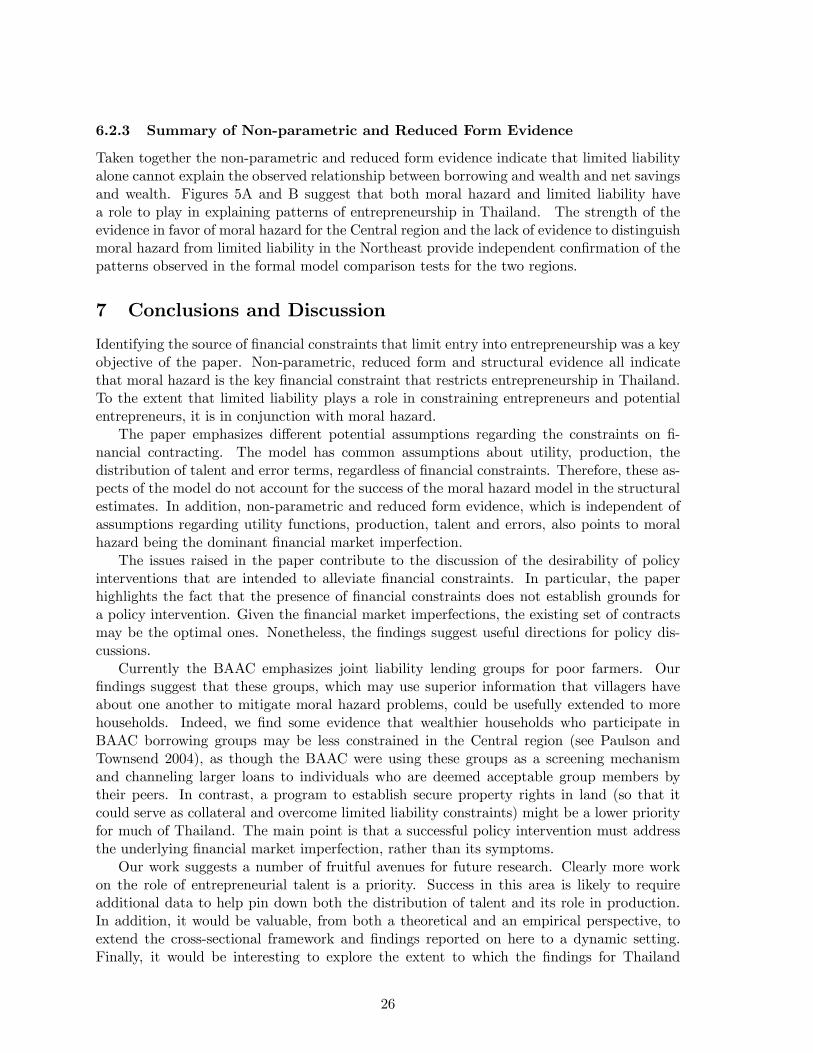
6.2.3 Summary of Non-parametric and Reduced Form Evidence

Taken together the non-parametric and reduced form evidence indicate that limited liabilityalone cannot explain the observed relationship between borrowing and wealth and net savingsand wealth. Figures 5A and B suggest that both moral hazard and limited liability havea role to play in explaining patterns of entrepreneurship in Thailand. The strength of theevidence in favor of moral hazard for the Central region and the lack of evidence to distinguishmoral hazard from limited liability in the Northeast provide independent confirmation of thepatterns observed in the formal model comparison tests for the two regions.

7 Conclusions and Discussion

Identifying the source of financial constraints that limit entry into entrepreneurship was a keyobjective of the paper. Non-parametric, reduced form and structural evidence all indicatethat moral hazard is the key financial constraint that restricts entrepreneurship in Thailand.To the extent that limited liability plays a role in constraining entrepreneurs and potentialentrepreneurs, it is in conjunction with moral hazard.

The paper emphasizes different potential assumptions regarding the constraints on fi-nancial contracting. The model has common assumptions about utility, production, thedistribution of talent and error terms, regardless of financial constraints. Therefore, these as-pects of the model do not account for the success of the moral hazard model in the structuralestimates. In addition, non-parametric and reduced form evidence, which is independent ofassumptions regarding utility functions, production, talent and errors, also points to moralhazard being the dominant financial market imperfection.

The issues raised in the paper contribute to the discussion of the desirability of policyinterventions that are intended to alleviate financial constraints. In particular, the paperhighlights the fact that the presence of financial constraints does not establish grounds fora policy intervention. Given the financial market imperfections, the existing set of contractsmay be the optimal ones. Nonetheless, the findings suggest useful directions for policy dis-cussions.

Currently the BAAC emphasizes joint liability lending groups for poor farmers. Ourfindings suggest that these groups, which may use superior information that villagers haveabout one another to mitigate moral hazard problems, could be usefully extended to morehouseholds. Indeed, we find some evidence that wealthier households who participate inBAAC borrowing groups may be less constrained in the Central region (see Paulson andTownsend 2004), as though the BAAC were using these groups as a screening mechanismand channeling larger loans to individuals who are deemed acceptable group members bytheir peers. In contrast, a program to establish secure property rights in land (so that itcould serve as collateral and overcome limited liability constraints) might be a lower priorityfor much of Thailand. The main point is that a successful policy intervention must addressthe underlying financial market imperfection, rather than its symptoms.

Our work suggests a number of fruitful avenues for future research. Clearly more workon the role of entrepreneurial talent is a priority. Success in this area is likely to requireadditional data to help pin down both the distribution of talent and its role in production.In addition, it would be valuable, from both a theoretical and an empirical perspective, toextend the cross-sectional framework and findings reported on here to a dynamic setting.Finally, it would be interesting to explore the extent to which the findings for Thailand

26

generalize to other developing and developed countries.

References

[1] Abbring, Jaap, Pierre Andre Chiappori, James Heckman and Jean Pinquet. “AdverseSelection and Moral Hazard in Insurance: Can Dynamic Data Help to Distinguish?”Journal of the European Economic Association, 2003, Volume 1(Issue 2/3): 512-521.

[2] Aghion, Phillippe and Patrick Bolton. “A Trickle-down Theory of Growth and Develop-ment with Debt Overhang.” Review of Economic Studies (1996).

[3] Binford, Michael, Tae Jeong Lee and Robert Townsend. “Sampling Design for an Inte-grated Socioeconomic and Ecologic Survey Using Satellite Remote Sensing and Ordina-tion.” Manuscript. Chicago: University of Chicago, 2001.

[4] Blanchflower, D. and A. Oswald. “What Makes an Entrepreneur?” Journal of LaborEconomics, 16(1998): 26-60.

[5] Buera, Francisco. “Identification of and Testable Implications of Occupational ChoiceModels.” Manuscript. Chicago: University of Chicago, 2002.

[6] Buera, Francisco. “A Dynamic Model of Entrepreneurial Choice with Borrowing Con-straints.” Manuscript. Chicago: University of Chicago, 2002.

[7] Cunha, Flavio, James Heckman and Salvador Navarro. “Separating Uncertainty fromHeterogeneity in Life Cycle Earnings.” IZA Discussion Paper #1437, December 2004.

[8] Evans, David S. and Boyan Jovanovic. “An Estimated Model of Entrepreneurial Choiceunder Liquidity Constraints.” Journal of Political Economy 97 (1989): 808 - 827.

[9] Fafchamps, Marcel. “Sequential Labor Decisions Under Uncertainty: an EstimableHousehold Model of West African Farmers.” Econometrica 61(5) (1993): 1173-1197.

[10] Feder, Gershon et. al. Land Policies and Farm Productivity in Thailand. Baltimore:Johns Hopkins University Press, 1988.

[11] Gine, Xavier and Robert Townsend, “Evaluation of Financial Liberalization: A gen-eral equilibrium model with constrained occupation choice.” Journal of DevelopmentEconomics, 2004.

[12] Gine, Xavier. “Access to Capital in Rural Thailand: An Estimated Model of Formal vs.Informal Credit.” World Bank Working Paper #3502, 2005.

[13] Greenwood, Jeremy and Boyan Jovanovic. “Financial Development, Growth, and theDistribution of Income.” Journal of Political Economy 98 (1990): 1076 - 1107.

[14] Holtz-Eakin, Douglas, Joulfian, David and Harvey S. Rosen. “Sticking It Out: En-trepreneurial Survival and Liquidity Constraints.” Journal of Political Economy 102(1994): 53 - 75.

27

[15] Jeong, Hyeok and Robert Townsend. “Household Businesses and their Financing inSemi-Urban and Rural Thailand.” Manuscript. Chicago: University of Chicago, 1998.

[16] Judd, Kenneth, “Numerical Methods In Economics”, MIT Press, Cambridge, MA, 1998.

[17] Kaboski, Joseph and Robert Townsend. “Borrowing and Lending in Semi-Urban andRural Thailand.” Manuscript. Chicago: University of Chicago, 1998.

[18] Karaivanov, Alexander. “Incomplete Financial Markets and Occupational Choice: Evi-dence from Thai Villages.” Manuscript. Simon Fraser University, 2005.

[19] Lloyd-Ellis, Huw and Dan Bernhardt, “Enterprise, Inequality and Economic Develop-ment.” Review of Economic Studies 67 (2000): 147 - 168.

[20] Magnac, Thierry and Jean-Marc Robin, “Occupational Choice and Liquidity Con-straints.” Richerche Economiche (1996) 50: 105 - 133.

[21] Paulson, Anna L. and Robert Townsend “Entrepreneurship and Financial Constraintsin Thailand.” Journal of Corporate Finance (2004) Vol 10 No 2 229-262..

[22] Petersen, Mitchell A. and Raghuram G. Rajan. “The Benefits of Lender Relationships:Evidence from Small Business Data.” Journal of Finance 49 (March 1994): 3 -37.

[23] Petersen, Mitchell A. and Raghuram G. Rajan. “The Effect of Credit Market Com-petition on Lending Relationships.” Quarterly Journal of Economics 110 (May 1995):407-444.

[24] Phelan, Christopher and Robert Townsend. “Computing Multi-Period, Information-Constrained Equilibria.” Review of Economic Studies 58 (1991): 853-881.

[25] Prescott, Edward and Robert Townsend. “Pareto Optima and Competitive Equilibriawith Adverse Selection and Moral Hazard.” Econometrica 152 (January 1984): 21-45.

[26] Seiler, Edward and Robert Townsend. “Assets in Semi-Urban and Rural Thailand.”Manuscript. Chicago: University of Chicago, 1998.

[27] Townsend, Robert principal investigator with Anna Paulson, Sombat Sakuntasathien,Tae Jeong Lee and Michael Binford. “Questionnaire design and data collection forNICHD grant ‘Risk, Insurance and the Family’ and NSF grants”, 1997.

[28] Townsend, Robert and Jacob Yaron. “The Credit Risk-Contingency System of An AsianDevelopment Bank”, Economic Perspectives, Federal Reserve Bank of Chicago, 2001.

[29] Vuong, Quang H. “Likelihood Ratio Tests for Model Selection and Non-nested Hypothe-ses.” Econometrica, Volume 57, Issue 2, (March 1989): 307-333.

[30] Wolak, Frank. “Estimating Regulated Firm Production Functions with Private Informa-tion: An Application to California Water Utilities.” Annales d’Economie et de Statistique(1994) 34: 13-69.

28

Figure 1: Lowess Estimates of the Probability of Being an Entrepreneur and Wealth500 bootstrap estimates of the relationship between being an entrepreneur and wealth were created using a bandwidth of 0.8. The 2.5th percentile (dashed line), 5th percentile (dashed line) median (solid line), 95th

percentile (dashed line) and 97.5th percentile (dashed line) estimates are shown in the figure.

0.2

.4.6

.8P

roba

bilit

y of

Ent

repr

eneu

rshi

p

0 .2 .4 .6 .8 1Wealth

2.5th percentile 5th percentilemedian 97.5th percentile95th percentile

0

1

2

0 0.1 0.2 0.3 0.4 0.5 0.6 0.7 0.8 0.9 1 1.1 1.2 1.3

capital, k

effo

rt, z

First Best k=0.42, z=1.69, welfare=0.448

Moral Hazard k=0.38, z=0.99, welfare=0.434

Limited Liability k=0.25, z=1.44 welfare=0.413

Both LL & MH k=0.25, z=1.04 welfare=0.409

Figure 2: Assignments of Capital (k) and Effort (z) for the Entrepreneurs in the Risk Neutral Model Moral Hazard, Limited Liability and Both Moral Hazard and Limited Liability

assumptions: θ=2.56, A = 0.10, α=0.78, κ=0.08, γ2=1.00, r=1.10, λ = 2.50

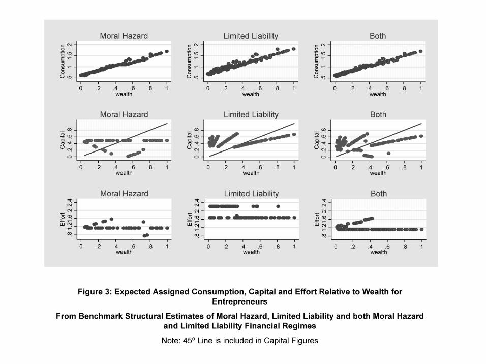
Table 1: Summary Statistics Whole Sample Northeast Central Variables used in Structural and Reduced Form/Non-parametric Estimation (All Households) Number of Households 2,313 1,209 1,104 % Business Households 14% 9% 19% Years of Schooling All Households 4.03

(2.56) 3.97

(2.45) 4.09

(2.67) Business Households 4.70

(2.90) 5.00

(3.00) 4.50

(2.80) Wealth Six Years Prior to survey All Households 1,007,166

(3,929,520) 355,996

(648,590) 1,712,046

(5,545,901) Business Households 2,532,464

(7,603,877) 428,490

(558,630) 3,614,755

(9,168,505) Constrained Business Households* 1,199,500

(5,770,877) 313,093

(546,497) 1,655,471

(7,051,744) Unconstrained Business Households 1,562,854

(5,550,756) 137,406

(343,281) 2,296,109

(6,713,852) Variables used in Reduced Form/Non-parametric Estimation (Business Households Only) Number of Households 361 122 239 Initial Business Investment 148,734

(339,562) 81,311

(176,918) 179,349

(388,312) Net Savings 4,562

(714,701) -13,680

(410,166) 13,946

(829,564) % who are net borrowers 55% 61% 51% % who report they are constrained* 56% 68% 50% Age of Head 49.5

(13.9) 48.4

(13.6) 50.1

(14.1) # of Adult Females in the Household

1.6 (0.9)

1.6 (0.8)

1.7 (0.9)

# of Adult Males in the Household 1.6 (0.9)

1.5 (0.9)

1.7 (0.9)

# of Children (< 18 years) in the Household

1.5 (1.2)

1.5 (1.1)

1.6 (1.3)

% of Business Households who were Member/Customer of Organization/Institution Six Years Ago Formal Financial Inst. 23% 16% 27% Village Inst./Org 11% 10% 12% Agricultural Lender 33% 33% 33% BAAC Group 22% 29% 18% Money Lender 4% 5% 4% Notes: Standard errors in parentheses. Wealth is in Thai Baht. The exchange rate at the time of the survey is 25 Baht to $1. *Households who reported that their businesses would be more profitable if it were expanded are labeled “constrained”. Households who report that their business would not be more profitable if it were expanded are labeled “unconstrained”.

Table 2: Parameter Values from Structural Estimation, Whole Sample Bootstrap Standard Errors in Parentheses

Moral Hazard Limited Liability Both 1. Risk Aversion, Talent (Income) γ1 0.0985

(0.0125) 0.0982

(0.0003) 0.1025

(0.0046) γ2 2.1007

(0.3216) 1.1713

(0.0037) 2.4753

(0.1797) κ 0.1257

(0.0227) 0.1079

(0.0003) 0.1190

(0.0062) α 0.7775

(0.0325) 0.6937

(0.0165) 0.7208

(0.0108) λ -- 22.9885

(0.0727) 20.8082 (1.4882)

2. Risk Neutral, Talent (Income) γ2 1.5801

(0.0243) 1.3475

(0.0167) 1.5511

(0.0171) κ 0.0530

(0.0009) 0.0675

(0.0009) 0.0789

(0.0008) α 0.7700

(0.0099) 0.6800

(0.0273) 0.6902

(0.0043) λ -- 24.5000

(0.3307) 28.3848 (0.3095)

3. Risk Aversion, Talent (% Entrepreneur) γ1 1.0737

(0.0123) 0.0668

(0.0004) 0.7781

(0.0035) γ2 1.0000

(0.0192) 1.0000

(0.0141) 1.0000

(0.0105) κ 0.0904

(0.0001) 0.0722

(0.0001) 0.1219

(0.0016) α 0.9780

(0.0032) 0.9702

(0.0003) 0.5062

(0.0066) λ 10.7281

(0.0305) 1.9014

(0.0042) 4. Risk Aversion, Estimated Talent γ1 0.5753

(0.0175) 0.0957

(0.0002) 0.1002

(0.0005) γ2 1.0494

(0.0171) 1.2314

(0.0120) 1.0939

(0.0061) κ 1.2312

(0.0649) 0.9889

(0.0049) 1.0022

(0.0065) α 0.7931

(0.0148) 0.2283

(0.0030) 0.7985

(0.0188) δ0 1.0175

(0.0464) 0.8853

(0.0108) 0.1002

(0.0007) δ1 0.0604

(0.0218) 0.0285

(0.0002) 0.0503

(0.0004) δ2 0.0516

(0.0053) -0.2226

(0.0046) 0.3005

(0.0018) λ -- 21.0118

(0.2223) 5.0088

(0.0970)

Table 3: Log Likelihoods from Structural Estimation A. Whole Sample Moral Hazard Limited Liability Both Risk Aversion, Talent (Income)

-0.4038 -0.4706 -0.4683

Risk Neutral, Talent (Income)

-0.4104 -0.4608 -0.4372

Risk Aversion, Talent (% Entrepreneur)

-0.4590 -0.7514 -0.6064

Risk Aversion, Estimated Talent -0.3996 -0.4134 -0.4035 B. Northeast Moral Hazard Limited Liability Both Risk Aversion, Talent (Income)

-0.3044 -0.3474 -0.3258

Risk Neutral, Talent (Income)

-0.3046 -0.3474 -0.3474

Risk Aversion, Talent (% Entrepreneur)

-0.3408 -0.4588 -0.4250

Risk Aversion, Estimated Talent -0.3040 -0.3045 -0.3029 C. Central Moral Hazard Limited Liability Both Risk Aversion, Talent (Income)

-0.5014 -0.5966 -0.5668

Risk Neutral, Talent (Income)

-0.5190 -0.5966 -0.5553

Risk Aversion, Talent (% Entrepreneur)

-0.6104 -0.8658 -0.7902

Risk Aversion, Estimated Talent -0.4991 -0.5355 -0.5185

Table 4: Comparison of Financial Regimes, Vuong Test Results A. Whole Sample MH v. LL MH v. Both LL v. Both Best Overall

Fit Risk Aversion, Talent (Income)

MH*** (0.0000)

MH*** (0.0001)

Both (0.8866)

MH

Risk Neutral, Talent (Income)

MH*** (0.0010)

MH** (0.0252)

Both*** (0.0033)

MH

Risk Aversion, Talent (% Entrepreneur)

MH*** (0.0000)

MH*** (0.0000)

Both*** (0.0000)

MH

Risk Aversion, Estimated Talent MH*** (0.0046)

MH (0.3402)

Both*** (0.0046)

MH or Both

B. Northeast MH v. LL MH v. Both LL v. Both Best Overall

Fit Risk Aversion, Talent (Income)

MH*** (0.0071)

MH* (0.0519)

Both*** (0.0081)

MH

Risk Neutral, Talent (Income)

MH*** (0.0073)

MH*** (0.0073)

Tie (0.1018)

MH

Risk Aversion, Talent (% Entrepreneur)

MH*** (0.0000)

MH*** (0.0012)

Both*** (0.0000)

MH

Risk Aversion, Estimated Talent MH (0.4213)

Both (0.3718)

Both (0.1846)

MH, LL or Both

C. Central MH v. LL MH v. Both LL v. Both Best Overall

Fit Risk Aversion, Talent (Income) MH***

(0.0003) MH***

(0.0008) Both

(0.1897) MH

Risk Neutral, Talent (Income)

MH*** (0.0007)

MH** (0.0263)

Both** (0.0133)

MH

Risk Aversion, Talent (High)

MH*** (0.0000)

MH*** (0.0000)

Both*** (0.0027)

MH

Risk Aversion, Estimated Talent MH*** (0.0004)

MH** (0.0426)

Both (0.1342)

MH

Note: MH = Moral Hazard, LL = Limited Liability, Both = Moral Hazard and Limited Liability. The abbreviation for model which best fits the data in the pairwise comparison is reported. The p-value for the Vuong tests are in parentheses. *** indicates significance at at least the one percent level, ** at at least the 5% level and * at at least the 10% level.

Tab

le 5

A: P

robi

t Est

imat

es o

f Bei

ng a

Net

Bor

row

er (N

et S

avin

gs <

0),

Bus

ines

s Hou

seho

lds

W

hole

Sam

ple

Nor

thea

st

Cen

tral

Reg

ion

dF

/dx*

Z-

stat

istic

dF

/dx*

Z-

stat

istic

dF

/dx*

Z-

stat

istic

C

onst

rain

ed (=

1 if

con

stra

ined

, 0 o

ther

wis

e)*

0.08

491.

55-0

.049

1 -0

.48

0.13

211.

97W

ealth

Six

Yea

rs a

go†

-0.0

013

-0.2

40.

1880

1.

750.

0007

0.12

Age

of H

ead

-0.0

115

-0.8

2-0

.014

9 -0

.58

-0.0

116

-0.6

7A

ge o

f Hea

d Sq

uare

d 0.

0001

0.65

0.00

01

0.47

0.00

010.

49Y

ears

of S

choo

ling

– H

ead

0.00

490.

47-0

.002

7 -0

.16

0.00

100.

07#

of A

dult

Fem

ales

in h

ouse

hold

0.

0494

1.37

0.13

20

1.81

0.02

680.

62#

of A

dult

Mal

es in

hou

seho

ld

-0.0

701

-2.0

5-0

.183

8 -2

.64

-0.0

334

-0.8

2#

of C

hild

ren

(< 1

8 ye

ars)

in h

ouse

hold

0.

0344

1.47

0.13

38

2.63

0.00

590.

21

O

bser

ved

Freq

uenc

y 0.

5457

0.60

66

0.51

46Pr

edic

ted

Freq

uenc

y at

mea

n of

X

0.54

830.

6367

0.

5153

Log

Like

lihoo

d -2

37.0

2-7

0.50

-1

58.4

7Ps

eudo

R-s

quar

ed

4.70

%13

.79%

4.

28%

Num

ber o

f Obs

erva

tions

36

112

2 23

9N

et sa

ving

s is d

efin

ed to

be

finan

cial

ass

ets p

lus l

oans

ow

ned

to h

ouse

hold

min

us d

ebt.

Dum

my

varia

bles

are

mar

ked

by a

n as

teris

k. †

Wea

lth si

x ye

ars a

go is

m

ade

up o

f the

val

ue o

f hou

seho

ld a

sset

s, ag

ricul

tura

l ass

ets a

nd la

nd.

Num

ber i

n ta

ble

is e

stim

ated

coe

ffic

ient

mul

tiplie

d by

1,0

00,0

00.

The

sam

ple

excl

udes

th

e to

p 1%

of h

ouse

hold

s by

wea

lth.

The

est

imat

es a

lso

incl

ude

cont

rols

for p

ast m

embe

rshi

p/pa

trona

ge o

f var

ious

fina

ncia

l ins

titut

ions

and

org

aniz

atio

ns.

Tab

le 5

B: R

egre

ssio

n E

stim

ates

of N

et S

avin

gs, B

usin

ess H

ouse

hold

s

Who

le S

ampl

e N

orth

east

C

entr

al R

egio

n

Coe

ff.

T-st

atis

tic

Coe

ff.

T-st

atis

tic

Coe

ff.

T-st

atis

tic

Wea

lth S

ix Y

ears

ago

– C

onst

rain

ed B

usin

ess†

0.

048

4.32

-0.0

04

0.05

0.04

83.

63W

ealth

Six

Yea

rs a

go –

Unc

onst

rain

ed B

usin

ess†

0.

012

1.42

0.38

3 3.

310.

012

1.19

Age

of H

ead

9592

.724

0.52

5639

.596

0.

2915

814.

300

0.60

Age

of H

ead

Squa

red

-93.

922

-0.5

6-7

1.27

2 -0

.41

-161

.393

-0.6

8Y

ears

of S

choo

ling

– H

ead

-231

79.8

90-1

.67

-122

83.4

10

-0.9

6-2

8433

.790

-1.3

5#

of A

dult

Fem

ales

in h

ouse

hold

-1

0587

5.20

0-2

.18

-133

223.

000

-2.5

9-1

0481

2.20

0-1

.56

# of

Adu

lt M

ales

in h

ouse

hold

10

8636

.700

2.37

6096

2.52

0 1.

2214

0117

.500

2.22

# of

Chi

ldre

n (<

18

year

s) in

hou

seho

ld

3771

0.18

01.

21-6

0660

.900

-1

.68

6476

1.76

01.

54C

onst

ant

-234

535.

400

-0.4

812

1595

.300

0.

25-4

6108

1.30

0-0

.65

Adj

uste

d R

-squ

ared

7.

86%

9.94

%

8.71

%N

umbe

r of O

bser

vatio

ns

361

122

239

Net

savi

ngs i

s def

ined

to b

e fin

anci

al a

sset

s plu

s loa

ns o

wne

d to

hou

seho

ld m

inus

deb

t. D

umm

y va

riabl

es a

re m

arke

d by

an

aste

risk.

†W

ealth

six

year

s ago

is

mad

e up

of t

he v

alue

of h

ouse

hold

ass

ets,

agric

ultu

ral a

sset

s and

land

. N

umbe

r in

tabl

e is

est

imat

ed c

oeff

icie

nt m

ultip

lied

by 1

,000

,000

. Th

e sa

mpl

e ex

clud

es

the

top

1% o

f hou

seho

lds b

y w

ealth

.

1

Working Paper Series

A series of research studies on regional economic issues relating to the Seventh Federal Reserve District, and on financial and economic topics.

Dynamic Monetary Equilibrium in a Random-Matching Economy WP-00-1 Edward J. Green and Ruilin Zhou The Effects of Health, Wealth, and Wages on Labor Supply and Retirement Behavior WP-00-2 Eric French Market Discipline in the Governance of U.S. Bank Holding Companies: WP-00-3 Monitoring vs. Influencing Robert R. Bliss and Mark J. Flannery Using Market Valuation to Assess the Importance and Efficiency of Public School Spending WP-00-4 Lisa Barrow and Cecilia Elena Rouse Employment Flows, Capital Mobility, and Policy Analysis WP-00-5 Marcelo Veracierto Does the Community Reinvestment Act Influence Lending? An Analysis of Changes in Bank Low-Income Mortgage Activity WP-00-6 Drew Dahl, Douglas D. Evanoff and Michael F. Spivey Subordinated Debt and Bank Capital Reform WP-00-7 Douglas D. Evanoff and Larry D. Wall The Labor Supply Response To (Mismeasured But) Predictable Wage Changes WP-00-8 Eric French For How Long Are Newly Chartered Banks Financially Fragile? WP-00-9 Robert DeYoung Bank Capital Regulation With and Without State-Contingent Penalties WP-00-10 David A. Marshall and Edward S. Prescott Why Is Productivity Procyclical? Why Do We Care? WP-00-11 Susanto Basu and John Fernald Oligopoly Banking and Capital Accumulation WP-00-12 Nicola Cetorelli and Pietro F. Peretto Puzzles in the Chinese Stock Market WP-00-13 John Fernald and John H. Rogers The Effects of Geographic Expansion on Bank Efficiency WP-00-14 Allen N. Berger and Robert DeYoung Idiosyncratic Risk and Aggregate Employment Dynamics WP-00-15 Jeffrey R. Campbell and Jonas D.M. Fisher

2

Working Paper Series (continued) Post-Resolution Treatment of Depositors at Failed Banks: Implications for the Severity of Banking Crises, Systemic Risk, and Too-Big-To-Fail WP-00-16 George G. Kaufman and Steven A. Seelig The Double Play: Simultaneous Speculative Attacks on Currency and Equity Markets WP-00-17 Sujit Chakravorti and Subir Lall Capital Requirements and Competition in the Banking Industry WP-00-18 Peter J.G. Vlaar Financial-Intermediation Regime and Efficiency in a Boyd-Prescott Economy WP-00-19 Yeong-Yuh Chiang and Edward J. Green How Do Retail Prices React to Minimum Wage Increases? WP-00-20 James M. MacDonald and Daniel Aaronson Financial Signal Processing: A Self Calibrating Model WP-00-21 Robert J. Elliott, William C. Hunter and Barbara M. Jamieson An Empirical Examination of the Price-Dividend Relation with Dividend Management WP-00-22 Lucy F. Ackert and William C. Hunter Savings of Young Parents WP-00-23 Annamaria Lusardi, Ricardo Cossa, and Erin L. Krupka The Pitfalls in Inferring Risk from Financial Market Data WP-00-24 Robert R. Bliss What Can Account for Fluctuations in the Terms of Trade? WP-00-25 Marianne Baxter and Michael A. Kouparitsas Data Revisions and the Identification of Monetary Policy Shocks WP-00-26 Dean Croushore and Charles L. Evans Recent Evidence on the Relationship Between Unemployment and Wage Growth WP-00-27 Daniel Aaronson and Daniel Sullivan Supplier Relationships and Small Business Use of Trade Credit WP-00-28 Daniel Aaronson, Raphael Bostic, Paul Huck and Robert Townsend What are the Short-Run Effects of Increasing Labor Market Flexibility? WP-00-29 Marcelo Veracierto Equilibrium Lending Mechanism and Aggregate Activity WP-00-30 Cheng Wang and Ruilin Zhou Impact of Independent Directors and the Regulatory Environment on Bank Merger Prices: Evidence from Takeover Activity in the 1990s WP-00-31 Elijah Brewer III, William E. Jackson III, and Julapa A. Jagtiani Does Bank Concentration Lead to Concentration in Industrial Sectors? WP-01-01 Nicola Cetorelli

3

Working Paper Series (continued) On the Fiscal Implications of Twin Crises WP-01-02 Craig Burnside, Martin Eichenbaum and Sergio Rebelo Sub-Debt Yield Spreads as Bank Risk Measures WP-01-03 Douglas D. Evanoff and Larry D. Wall Productivity Growth in the 1990s: Technology, Utilization, or Adjustment? WP-01-04 Susanto Basu, John G. Fernald and Matthew D. Shapiro Do Regulators Search for the Quiet Life? The Relationship Between Regulators and The Regulated in Banking WP-01-05 Richard J. Rosen Learning-by-Doing, Scale Efficiencies, and Financial Performance at Internet-Only Banks WP-01-06 Robert DeYoung The Role of Real Wages, Productivity, and Fiscal Policy in Germany’s Great Depression 1928-37 WP-01-07 Jonas D. M. Fisher and Andreas Hornstein Nominal Rigidities and the Dynamic Effects of a Shock to Monetary Policy WP-01-08 Lawrence J. Christiano, Martin Eichenbaum and Charles L. Evans Outsourcing Business Service and the Scope of Local Markets WP-01-09 Yukako Ono The Effect of Market Size Structure on Competition: The Case of Small Business Lending WP-01-10 Allen N. Berger, Richard J. Rosen and Gregory F. Udell Deregulation, the Internet, and the Competitive Viability of Large Banks WP-01-11 and Community Banks Robert DeYoung and William C. Hunter Price Ceilings as Focal Points for Tacit Collusion: Evidence from Credit Cards WP-01-12 Christopher R. Knittel and Victor Stango Gaps and Triangles WP-01-13 Bernardino Adão, Isabel Correia and Pedro Teles A Real Explanation for Heterogeneous Investment Dynamics WP-01-14 Jonas D.M. Fisher Recovering Risk Aversion from Options WP-01-15 Robert R. Bliss and Nikolaos Panigirtzoglou Economic Determinants of the Nominal Treasury Yield Curve WP-01-16 Charles L. Evans and David Marshall Price Level Uniformity in a Random Matching Model with Perfectly Patient Traders WP-01-17 Edward J. Green and Ruilin Zhou Earnings Mobility in the US: A New Look at Intergenerational Inequality WP-01-18 Bhashkar Mazumder

4

Working Paper Series (continued) The Effects of Health Insurance and Self-Insurance on Retirement Behavior WP-01-19 Eric French and John Bailey Jones The Effect of Part-Time Work on Wages: Evidence from the Social Security Rules WP-01-20 Daniel Aaronson and Eric French Antidumping Policy Under Imperfect Competition WP-01-21 Meredith A. Crowley Is the United States an Optimum Currency Area? An Empirical Analysis of Regional Business Cycles WP-01-22 Michael A. Kouparitsas A Note on the Estimation of Linear Regression Models with Heteroskedastic Measurement Errors WP-01-23 Daniel G. Sullivan The Mis-Measurement of Permanent Earnings: New Evidence from Social WP-01-24 Security Earnings Data Bhashkar Mazumder Pricing IPOs of Mutual Thrift Conversions: The Joint Effect of Regulation and Market Discipline WP-01-25 Elijah Brewer III, Douglas D. Evanoff and Jacky So Opportunity Cost and Prudentiality: An Analysis of Collateral Decisions in Bilateral and Multilateral Settings WP-01-26 Herbert L. Baer, Virginia G. France and James T. Moser Outsourcing Business Services and the Role of Central Administrative Offices WP-02-01 Yukako Ono Strategic Responses to Regulatory Threat in the Credit Card Market* WP-02-02 Victor Stango The Optimal Mix of Taxes on Money, Consumption and Income WP-02-03 Fiorella De Fiore and Pedro Teles Expectation Traps and Monetary Policy WP-02-04 Stefania Albanesi, V. V. Chari and Lawrence J. Christiano Monetary Policy in a Financial Crisis WP-02-05 Lawrence J. Christiano, Christopher Gust and Jorge Roldos Regulatory Incentives and Consolidation: The Case of Commercial Bank Mergers and the Community Reinvestment Act WP-02-06 Raphael Bostic, Hamid Mehran, Anna Paulson and Marc Saidenberg Technological Progress and the Geographic Expansion of the Banking Industry WP-02-07 Allen N. Berger and Robert DeYoung

5

Working Paper Series (continued) Choosing the Right Parents: Changes in the Intergenerational Transmission WP-02-08 of Inequality Between 1980 and the Early 1990s David I. Levine and Bhashkar Mazumder The Immediacy Implications of Exchange Organization WP-02-09 James T. Moser Maternal Employment and Overweight Children WP-02-10 Patricia M. Anderson, Kristin F. Butcher and Phillip B. Levine The Costs and Benefits of Moral Suasion: Evidence from the Rescue of WP-02-11 Long-Term Capital Management Craig Furfine On the Cyclical Behavior of Employment, Unemployment and Labor Force Participation WP-02-12 Marcelo Veracierto Do Safeguard Tariffs and Antidumping Duties Open or Close Technology Gaps? WP-02-13 Meredith A. Crowley Technology Shocks Matter WP-02-14 Jonas D. M. Fisher Money as a Mechanism in a Bewley Economy WP-02-15 Edward J. Green and Ruilin Zhou Optimal Fiscal and Monetary Policy: Equivalence Results WP-02-16 Isabel Correia, Juan Pablo Nicolini and Pedro Teles Real Exchange Rate Fluctuations and the Dynamics of Retail Trade Industries WP-02-17 on the U.S.-Canada Border Jeffrey R. Campbell and Beverly Lapham Bank Procyclicality, Credit Crunches, and Asymmetric Monetary Policy Effects: WP-02-18 A Unifying Model Robert R. Bliss and George G. Kaufman Location of Headquarter Growth During the 90s WP-02-19 Thomas H. Klier The Value of Banking Relationships During a Financial Crisis: WP-02-20 Evidence from Failures of Japanese Banks Elijah Brewer III, Hesna Genay, William Curt Hunter and George G. Kaufman On the Distribution and Dynamics of Health Costs WP-02-21 Eric French and John Bailey Jones The Effects of Progressive Taxation on Labor Supply when Hours and Wages are WP-02-22 Jointly Determined Daniel Aaronson and Eric French

6

Working Paper Series (continued) Inter-industry Contagion and the Competitive Effects of Financial Distress Announcements: WP-02-23 Evidence from Commercial Banks and Life Insurance Companies Elijah Brewer III and William E. Jackson III State-Contingent Bank Regulation With Unobserved Action and WP-02-24 Unobserved Characteristics David A. Marshall and Edward Simpson Prescott Local Market Consolidation and Bank Productive Efficiency WP-02-25 Douglas D. Evanoff and Evren Örs Life-Cycle Dynamics in Industrial Sectors. The Role of Banking Market Structure WP-02-26 Nicola Cetorelli Private School Location and Neighborhood Characteristics WP-02-27 Lisa Barrow Teachers and Student Achievement in the Chicago Public High Schools WP-02-28 Daniel Aaronson, Lisa Barrow and William Sander The Crime of 1873: Back to the Scene WP-02-29 François R. Velde Trade Structure, Industrial Structure, and International Business Cycles WP-02-30 Marianne Baxter and Michael A. Kouparitsas Estimating the Returns to Community College Schooling for Displaced Workers WP-02-31 Louis Jacobson, Robert LaLonde and Daniel G. Sullivan A Proposal for Efficiently Resolving Out-of-the-Money Swap Positions WP-03-01 at Large Insolvent Banks George G. Kaufman Depositor Liquidity and Loss-Sharing in Bank Failure Resolutions WP-03-02 George G. Kaufman Subordinated Debt and Prompt Corrective Regulatory Action WP-03-03 Douglas D. Evanoff and Larry D. Wall When is Inter-Transaction Time Informative? WP-03-04 Craig Furfine Tenure Choice with Location Selection: The Case of Hispanic Neighborhoods WP-03-05 in Chicago Maude Toussaint-Comeau and Sherrie L.W. Rhine Distinguishing Limited Liability from Moral Hazard in a Model of Entrepreneurship∗ WP-03-06 Alexander Karaivanov, Anna L. Paulson and Robert Townsend