1

Distance Correlation for Vectors: A SAS® Macro

Thomas E. Billings, MUFG Union Bank, N.A., San Francisco, California

This work by Thomas E. Billings is licensed (2016) under a Creative Commons Attribution 4.0 International License.

ABSTRACT

The Pearson correlation coefficient is well-known and widely-used. However, it suffers from certain constraints: it is a measure of linear dependence (only) and does not provide a test of statistical independence, and it is restricted to univariate random variables. Since its inception, related and alternative measures have been proposed to mitigate these constraints. Several new measures to replace or supplement Pearson correlation have been proposed in the statistical literature in recent years. Székeley et al. (2007) describes a new measure - distance correlation - that overcomes the shortcomings of Pearson correlation. Distance correlation is defined for 2 random variables X, Y (which can be vectors) as a weight or distance function applied to the difference between the joint characteristic function for (X,Y) and the product of the individual characteristic functions for X, Y. In practice it is estimated by computing the individual distance matrices for X, Y, and distance correlation is a similarity measure for the 2 matrices. For the bivariate normal case, distance correlation is a function of Pearson correlation. Distance correlation also supports a related test of statistical independence, and has performed well in simulation studies comparing it with other alternatives to Pearson correlation. Here we present a Base SAS

® macro

to compute distance correlation for arbitrary real vectors.

BACKGROUND: PEARSON CORRELATION COEFFICIENT AND ALTERNATIVES

The Pearson correlation coefficient is the most common and widely used correlation measure, supported in virtually all major statistical software systems. It has a (very) close association with the method of linear regression. The coefficient was derived by Karl Pearson, based on work done by Francis Galton in the 1880’s. The coefficient is defined as: ρ = CORR(X,Y) = Covariance(X,Y) / (SD(X)*SD(Y)) where: SD(*) = standard deviation(*) = sqrt( variance(*) ). The R

2 statistic commonly computed in linear regression is the square of the Pearson correlation between

the dependent variable (Y) and the fitted regression estimates. The Pearson correlation coefficient has a number of major constraints:

• it is defined for univariate random variables only, and • it does not serve as a measure of general statistical dependence or independence; instead it is

primarily a measure of linear dependence. Regarding the latter point, the standard example found in some statistical texts is: let Y = X

2; then

cov(X,Y)=0 even though Y is a function of X; e.g., see DeGroot (1975).

2

Numerous measures have been proposed as alternatives to overcome some of the limitations of Pearson correlation. Alternatives date back many years and are not limited to recent efforts. Some examples that are supported in SAS

® PROC CORR include the following:

• Spearman rank, • Kendall’s tau-b, • Hoeffding’s D statistic.

PROC CORR also supports partial and polychoric correlation measures. Some interesting alternative statistics proposed in recent years include:

• Maximal information coefficient (Reshef et al. 2011) - prematurely and incorrectly promoted as “a correlation for the 21

st century” by Terry Speed (2011); however subsequent research reveals it is

badly flawed, to say the least – see Kinney & Atwal (2014), Simon & Tibshirani (2014); • Mutual information – Kullback-Leibler divergence between the joint probability distribution for

(X,Y) and the product of the individual probability distributions for X, Y; • Copula correlation (Ding & Li 2013); • Distance correlation (Székeley et al. 2007)

and variations of the above statistics. There is a rich statistical literature on correlation and related association measures; the above is just a sample – additional measures have been proposed in the literature. Simulation studies comparing alternative measures show mixed results based on differences in methodology and sample sizes. However a number of studies that use data with noise suggest that distance correlation may be the best of the recent alternatives; Simon & Tibshirani (2014), also see Clark (2013). DISTANCE CORRELATION Distance correlation is a new measure (first described in 2007 and expanded in 2009) that overcomes the major limitations of Pearson correlation, i.e.:

• it is defined for random variables of arbitrary dimension – in fact X & Y can have different dimensions so long as you use a conformable weight or distance function, and

• it provides/supports a test of general statistical independence The basic properties of the measure are:

• It is defined in the closed interval [0,1]; in contrast, Pearson correlation is defined in the closed interval [-1,1] and

• for the bivariate normal case, distance correlation is a function of the Pearson correlation ρ Formal definition. Consider 2 sequences of real-valued vectors Xi, Yi, i=1,…,n; X has dimension p, Y has dimension q, where p, q are positive integers. It is possible that p=q but this is not required. At this stage we digress to remind readers of some basics: the characteristic function is defined as f(t) = E(e

itX)

aka the Fourier-Stieltjes transform of the CDF (cumulative distribution function) F. For additional background on characteristic functions, see Chung (1974).

3

Now let fx, fy denote the characteristic functions for random variables X,Y with only 1 limitation: X and Y both have finite first moments (euclidean norm). Distance covariance is defined as dcov(X,Y) = || fx,y (t,s) – fx(t)fy(s)||

2w

where ||*|| denotes an arbitrary complex positive weight (distance) function defined in R

p+q that is

integrable in L2. Distance variance – denoted as dvar(*) has the similar obvious definition, substituting X for Y in the above. Similar to Pearson correlation we then define the distance correlation between X and Y as: dcor(X,Y) = dcov(X,Y) / (sqrt( dvar(X)*dvar(Y) )) (1) Note that distance covariance and correlation can be defined without use of characteristic functions. Lyons (2013) characterizes the metric spaces where distance correlation supports a test of independence as being of “strong negative type” where “negative type is equivalent to a certain property of embeddability into Hilbert space”. Interested readers are encouraged to review Lyons (2013) for details. Estimators. Simplifying the notation somewhat, let X,Y be real-valued vector sequences with n rows that have no missing values. X & Y can be the same or different dimensions, and rows with missing values can be filtered out or filled with proxy values. Let: akl = |Xk – Xl|p = distance between rows k & l in the X variable vector sequence. Construct an n X n distance matrix with all values of akl, This will be a symmetric matrix with a zero diagonal. Define marginal and grand means for the distance matrix in the usual way – i.e., ak. a.l a..; then define the adjusted distance matrix for X: Akl = akl – ak. – a.l + a.. Define a similar distance matrix for the Y variable vector sequence, denoted as bkl and Bkl The estimator for distance covariance is then: dcov(X,Y) = n

-2 * ∑(Akl * Bkl)

and dvar(z) has the similar definition setting X=Y=z. Distance correlation is then estimated using the estimators for dcov and dvar in equation (1) above. A statistic that provides a test of independence based on distance correlation is also available and described in theorem 6 of Székeley et al. (2007). A less technical way to describe distance correlation is as follows:

• Given 2 random variables X, Y which can be vectors or other non-univariate variables, • construct the square distance matrix for each variable; • distance correlation is then a measure of the similarity between the 2 distance matrices, i.e., • are the se of changes in distance between say rows k & l, similar across the 2 distance matrices?

IMPLEMENTATION IN SAS The estimators for distance correlation require the computation of multiple matrices and marginal vectors, and could easily be done in SAS/IML. However:

• SAS/IML is not widely used or available (most commercial sites do not have the product licensed), and

• SAS/IML is an old and dated product compared to open-source alternatives.

4

Instead, the Base SAS product is used here as everyone has it. The general processing outline is:

1. compute distance matrices using PROC DISTANCE; 2. marginals, sums, grand means are computed using PROC SUMMARY; 3. DATA steps are used for other calculations, and 4. encapsulate the code for parts 1-3 above in macros to support custom applications.

A set of SAS macros was developed for this project:

• Given a data set, compute square distance matrix for selected variables (Euclidean distance); macro %raw_dist_mtx

• Given a data set, compute marginal means, sums, and also grand means, sums; macro %mgn_plus,

• Given distance matrices and marginals, computed adjusted distance matrices per algorithm; macro %int_adj_matrices,

• Given distance matrices in data sets, compute the distance correlation and associated test statistic for a user-specified critical value; macro %dist_corr.

Code for the macros above can be found in the Appendix. The code is released under the BSD 2-clause open-source license which allows reuse for both commercial and non-commercial applications.

VALIDATION – COMPARE TO R DCOR FUNCTION

While the computations required for the estimator are straightforward, savvy readers will understand that errors are (always) possible in implementation, so can we validate the SAS macros against another calculation of distance correlation? The answer is yes: distance correlation is available in R package energy (Rizzo and Székeley, 2014), with R functions developed and checked by the same team that wrote the 2007 paper. Next, we need a data set to compute distance correlation with, using both SAS and R. The well-known “iris” data set is available in R and also in SAS help file: sashelp.iris. We choose here to use the iris data from R rather than from SAS, for copyright reasons. To explain the preceding: data are facts and cannot be copyrighted, but the arrangement of data can be copyrighted and/or in some countries may have sui generis rights which are similar to copyright. Comparing the iris data in R vs. SAS, we observe that the rows are in different order and some of the variables are scaled differently. The presumption here is that SAS Institute claims the “all rights reserved” copyright on the arrangement of the data in the help file, while in contrast the R data are copyright-free. For these reasons we use the iris data from R and export that from R and then import it into SAS for the validation. The 1

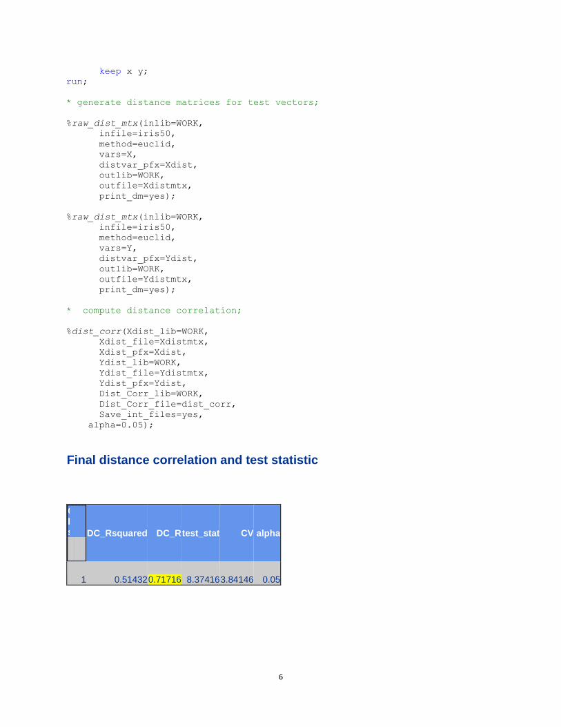
st 50 rows of R iris data were used to derive dcor in both R and in SAS. The values produced in

each software system matched. R code/output and SAS code/output are given below. * The SAS & R example program code below is released under a Berkeley

Systems Distribution BSD-2-Clause license, an open-source license which

permits free reuse and republication under conditions. The full license

is in the Appendix.;

5

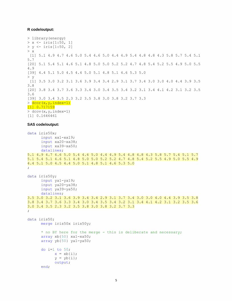
R code/output: > library(energy)

> x <- iris[1:50, 1]

> y <- iris[1:50, 2]

> x

[1] 5.1 4.9 4.7 4.6 5.0 5.4 4.6 5.0 4.4 4.9 5.4 4.8 4.8 4.3 5.8 5.7 5.4 5.1

5.7

[20] 5.1 5.4 5.1 4.6 5.1 4.8 5.0 5.0 5.2 5.2 4.7 4.8 5.4 5.2 5.5 4.9 5.0 5.5

4.9

[39] 4.4 5.1 5.0 4.5 4.4 5.0 5.1 4.8 5.1 4.6 5.3 5.0

> y

[1] 3.5 3.0 3.2 3.1 3.6 3.9 3.4 3.4 2.9 3.1 3.7 3.4 3.0 3.0 4.0 4.4 3.9 3.5

3.8

[20] 3.8 3.4 3.7 3.6 3.3 3.4 3.0 3.4 3.5 3.4 3.2 3.1 3.4 4.1 4.2 3.1 3.2 3.5

3.6

[39] 3.0 3.4 3.5 2.3 3.2 3.5 3.8 3.0 3.8 3.2 3.7 3.3

> dcor(x,y,index=1)

[1] 0.717159

> dcov(x,y,index=1)

[1] 0.1646461

SAS code/output: data iris50x;

input xa1-xa19;

input xa20-xa38;

input xa39-xa50;

datalines;

5.1 4.9 4.7 4.6 5.0 5.4 4.6 5.0 4.4 4.9 5.4 4.8 4.8 4.3 5.8 5.7 5.4 5.1 5.7

5.1 5.4 5.1 4.6 5.1 4.8 5.0 5.0 5.2 5.2 4.7 4.8 5.4 5.2 5.5 4.9 5.0 5.5 4.9

4.4 5.1 5.0 4.5 4.4 5.0 5.1 4.8 5.1 4.6 5.3 5.0

;

data iris50y;

input ya1-ya19;

input ya20-ya38;

input ya39-ya50;

datalines;

3.5 3.0 3.2 3.1 3.6 3.9 3.4 3.4 2.9 3.1 3.7 3.4 3.0 3.0 4.0 4.4 3.9 3.5 3.8

3.8 3.4 3.7 3.6 3.3 3.4 3.0 3.4 3.5 3.4 3.2 3.1 3.4 4.1 4.2 3.1 3.2 3.5 3.6

3.0 3.4 3.5 2.3 3.2 3.5 3.8 3.0 3.8 3.2 3.7 3.3

;

data iris50;

merge iris50x iris50y;

* no BY here for the merge - this is deliberate and necessary;

array xb{50} xa1-xa50;

array yb{50} ya1-ya50;

do i=1 to 50;

x = xb{i};

y = yb{i};

output;

end;

6

keep x y;

run;

* generate distance matrices for test vectors;

%raw_dist_mtx(inlib=WORK,

infile=iris50,

method=euclid,

vars=X,

distvar_pfx=Xdist,

outlib=WORK,

outfile=Xdistmtx,

print_dm=yes);

%raw_dist_mtx(inlib=WORK,

infile=iris50,

method=euclid,

vars=Y,

distvar_pfx=Ydist,

outlib=WORK,

outfile=Ydistmtx,

print_dm=yes);

* compute distance correlation;

%dist_corr(Xdist_lib=WORK,

Xdist_file=Xdistmtx,

Xdist_pfx=Xdist,

Ydist_lib=WORK,

Ydist_file=Ydistmtx,

Ydist_pfx=Ydist,

Dist_Corr_lib=WORK,

Dist_Corr_file=dist_corr,

Save_int_files=yes,

alpha=0.05);

Final distance correlation and test statistic

Obs

DC_Rsquared DC_R test_stat CV alpha

1 0.51432 0.71716 8.37416 3.84146 0.05

7

CONSTRAINTS ON DISTANCE CORRELATION CALCULATIONS

1. Using the brute-force methods employed herein (straight from the 2007 paper), calculations for dcor require a number of operations of the magnitude O(n

2).

2. Square distance matrices are redundant and, with a “large” row count, can consume substantial memory.

3. Given 1-3, it follows that the current algorithm is not well-suited for big-data. 4. An alternate, more efficient – and also considerably more complex - computational algorithm is

now available (Huo et al. 2015). CONCLUSIONS

• The SAS macros developed herein are proof-of-concept and can be used to compute dcor if the row count/sample size n is not “too big”.

• Distance correlation outperforms many other alternatives to Pearson correlation, and elegantly extends the concept of correlation to vectors.

• Distance correlation provides a test of statistical independence for vectors; this is an important extension.

• Personal opinion: dcor deserves wide use. • Note that implementing distance correlation in SAS/STAT software has been suggested to SAS

Institute. It is unclear/unknown if it will ever be implemented.

APPENDIX 1: CODE FOR SAS MACROS TO COMPUTE DISTANCE CORRELATION

The macros below make heavy use of the SAS %unquote function. Much of the code runs OK without %unquote in SAS versions 9.2 and 9.4, but in the system used for testing and development – a 9.3 site - %unquote was needed to prevent parsing errors. The macros include prints that may produce voluminous output for large distance matrices; you may wish to disable or remove those prints when using the macros. * This program code is released under a Berkeley Systems Distribution

BSD-2-Clause license, an open-source license which permits free

reuse and republication under conditions;

/*

Copyright (c) 2016, Thomas E. Billings

All rights reserved.

Redistribution and use in source and binary forms, with or without

modification, are permitted provided that the following conditions are met:

1. Redistributions of source code must retain the above copyright notice,

this list of conditions and the following disclaimer.

2. Redistributions in binary form must reproduce the above copyright notice,

this list of conditions and the following disclaimer in the documentation

and/or other materials provided with the distribution.

THIS SOFTWARE IS PROVIDED BY THE COPYRIGHT HOLDERS AND CONTRIBUTORS "AS IS"

AND ANY EXPRESS OR IMPLIED WARRANTIES, INCLUDING, BUT NOT LIMITED TO, THE

IMPLIED WARRANTIES OF MERCHANTABILITY AND FITNESS FOR A PARTICULAR PURPOSE

ARE DISCLAIMED. IN NO EVENT SHALL THE COPYRIGHT HOLDER OR CONTRIBUTORS BE

LIABLE FOR ANY DIRECT, INDIRECT, INCIDENTAL, SPECIAL, EXEMPLARY, OR

8

CONSEQUENTIAL DAMAGES (INCLUDING, BUT NOT LIMITED TO, PROCUREMENT OF

SUBSTITUTE GOODS OR SERVICES; LOSS OF USE, DATA, OR PROFITS; OR BUSINESS

INTERRUPTION) HOWEVER CAUSED AND ON ANY THEORY OF LIABILITY, WHETHER IN

CONTRACT, STRICT LIABILITY, OR TORT (INCLUDING NEGLIGENCE OR OTHERWISE)

ARISING IN ANY WAY OUT OF THE USE OF THIS SOFTWARE, EVEN IF ADVISED OF THE

POSSIBILITY OF SUCH DAMAGE.

*/

%macro raw_dist_mtx(inlib=WORK,

infile=,

method=euclid,

vars=,

distvar_pfx=,

outlib=WORK,

outfile=,

print_dm=no);

%* Simple macro to create a square distance matrix using the input

file

and variables specified per the invocation parameters.;

%* this macro has some error checking but a production macro would

have more checks. users need to supply a valid input

file with names of numeric variables that are present in the file,

plus a

valid distance method for SAS PROC DISTANCE. Use of method=euclid

is suggested, but PROC DISTANCE supports other methods.

Note that this macro has been tested ONLY with euclid method.;

%* macro parameters:

inlib=, infile= LIBNAME, filename of input file with raw data

method= euclid or squeuclid or other distance function in PROC

DISTANCE

distvar_pfx= prefix for (output) distance variable names

outlib=, outfile= LIBNAME, filename of output file with distance

matrix

print_dm = yes or no, print or not print derived distance matrix;

%* parameter checks to set defaults or terminate;

%let inlib=%qtrim(%qleft(&inlib.));

%let infile=%qtrim(%qleft(&infile.));

%let outlib=%qtrim(%qleft(&outlib.));

%let outfile=%qtrim(%qleft(&outfile.));

%if (%length(&inlib.) = 0) or (%length(&infile.) = 0) or

(%length(&outlib.) = 0) or (%length(&outfile.) = 0) %then

%do;

%put ERROR: Input or output LIBNAME/filename not specified.

Macro terminated.;

%return;

%end;

%let vars=%qtrim(%qleft(&vars.));

%if (%length(&vars.) = 0) %then

%do;

%put ERROR: No variables specified for distance matrix

computation. Macro terminated.;

%return;

9

%end;

%let distvar_pfx=%qtrim(%qleft(&distvar_pfx.));

%if (%length(&distvar_pfx.) = 0) %then

%do;

%put ERROR: No prefix specified for variable names in

distance matrix. Macro terminated.;

%return;

%end;

%let method=%qtrim(%qleft(&method.));

%if (%length(&method.) = 0) %then

%let method=euclid;

%let print_dm=%upcase(%qtrim(%qleft(&print_dm.)));

%if (%length(&print_dm.) = 0) or (&print_dm. ne YES) %then

%let print_dm=NO;

proc distance method=&method. data=&inlib..&infile.

out=&outlib..&outfile.

prefix=&distvar_pfx. shape=square;

var interval (&vars.);

run;

%if (&print_dm. eq YES) %then

%do;

proc print data=&outlib..&outfile.;

title "Raw distance matrix for vector defined by:

&vars.";

run;

%end;

%mend;

%macro mgn_plus(nr=, inlib=, infile=, pfx=, outlib=, outfile=, mg_print=no);

%* utility macro used in computing distance correlation;

proc summary data=&inlib..&infile. nway;

%unquote(var &pfx.1-&pfx.&nr.);

%unquote(output out=marginals mean=mg&pfx.1-mg&pfx.&nr.

sum=sm&pfx.1-sm&pfx.&nr.);

run;

data %unquote(&outlib..&outfile.);

set marginals;

%unquote(grmn&pfx. = (mean(of mg&pfx.1-mg&pfx.&nr.)));

%unquote(grsm&pfx. = sum(of sm&pfx.1-sm&pfx.&nr.));

drop _type_ _freq_;

run;

%if %upcase(&mg_print. = YES) %then

%do;

proc print data=%unquote(&outlib..&outfile.);

10

title "Marginals for raw distance matrix:

&inlib..&infile.";

title2 "with grand sum and mean";

run;

%end;

%mend;

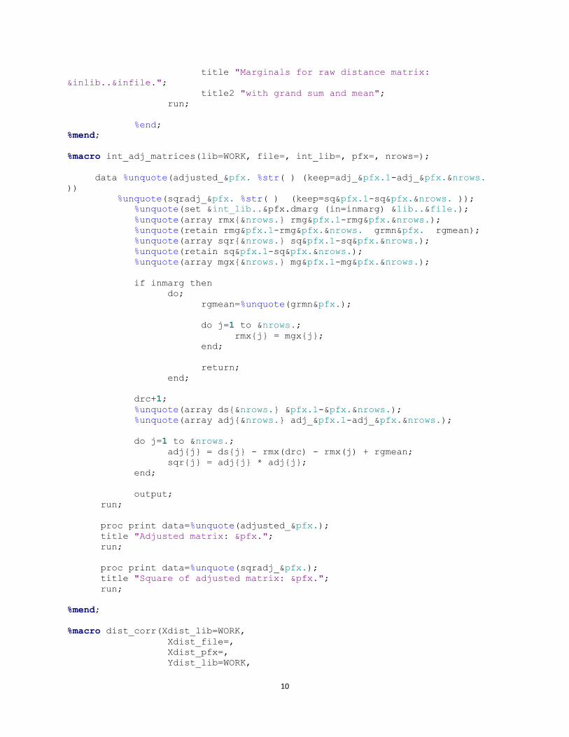
%macro int_adj_matrices(lib=WORK, file=, int_lib=, pfx=, nrows=);

data %unquote(adjusted_&pfx. %str( ) (keep=adj_&pfx.1-adj_&pfx.&nrows.

))

%unquote(sqradj_&pfx. %str( ) (keep=sq&pfx.1-sq&pfx.&nrows. ));

%unquote(set &int_lib..&pfx.dmarg (in=inmarg) &lib..&file.);

%unquote(array rmx{&nrows.} rmg&pfx.1-rmg&pfx.&nrows.);

%unquote(retain rmg&pfx.1-rmg&pfx.&nrows. grmn&pfx. rgmean);

%unquote(array sqr{&nrows.} sq&pfx.1-sq&pfx.&nrows.);

%unquote(retain sq&pfx.1-sq&pfx.&nrows.);

%unquote(array mgx{&nrows.} mg&pfx.1-mg&pfx.&nrows.);

if inmarg then

do;

rgmean=%unquote(grmn&pfx.);

do j=1 to &nrows.;

rmx{j} = mgx{j};

end;

return;

end;

drc+1;

%unquote(array ds{&nrows.} &pfx.1-&pfx.&nrows.);

%unquote(array adj{&nrows.} adj_&pfx.1-adj_&pfx.&nrows.);

do j=1 to &nrows.;

adj{j} = ds{j} - rmx(drc) - rmx(j) + rgmean;

sqr{j} = adj{j} * adj{j};

end;

output;

run;

proc print data=%unquote(adjusted_&pfx.);

title "Adjusted matrix: &pfx.";

run;

proc print data=%unquote(sqradj_&pfx.);

title "Square of adjusted matrix: &pfx.";

run;

%mend;

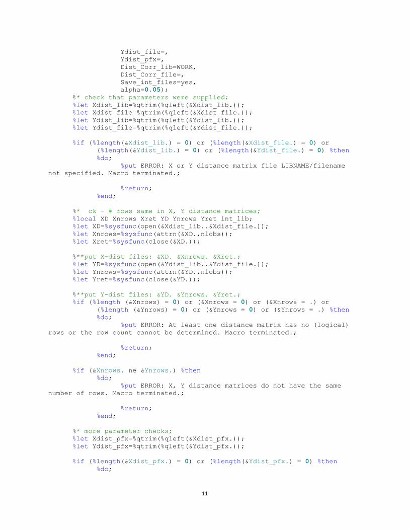
%macro dist_corr(Xdist_lib=WORK,

Xdist_file=,

Xdist_pfx=,

Ydist_lib=WORK,

11

Ydist_file=,

Ydist_pfx=,

Dist_Corr_lib=WORK,

Dist_Corr_file=,

Save_int_files=yes,

alpha=0.05);

%* check that parameters were supplied;

%let Xdist_lib=%qtrim(%qleft(&Xdist_lib.));

%let Xdist_file=%qtrim(%qleft(&Xdist_file.));

%let Ydist_lib=%qtrim(%qleft(&Ydist_lib.));

%let Ydist_file=%qtrim(%qleft(&Ydist_file.));

%if (%length(&Xdist_lib.) = 0) or (%length(&Xdist_file.) = 0) or

(%length(&Ydist_lib.) = 0) or (%length(&Ydist_file.) = 0) %then

%do;

%put ERROR: X or Y distance matrix file LIBNAME/filename

not specified. Macro terminated.;

%return;

%end;

%* ck - # rows same in X, Y distance matrices;

%local XD Xnrows Xret YD Ynrows Yret int_lib;

%let XD=%sysfunc(open(&Xdist_lib..&Xdist_file.));

%let Xnrows=%sysfunc(attrn(&XD.,nlobs));

%let Xret=%sysfunc(close(&XD.));

%**put X-dist files: &XD. &Xnrows. &Xret.;

%let YD=%sysfunc(open(&Ydist_lib..&Ydist_file.));

%let Ynrows=%sysfunc(attrn(&YD.,nlobs));

%let Yret=%sysfunc(close(&YD.));

%**put Y-dist files: &YD. &Ynrows. &Yret.;

%if (%length (&Xnrows) = 0) or (&Xnrows = 0) or (&Xnrows = .) or

(%length (&Ynrows) = 0) or (&Ynrows = 0) or (&Ynrows = .) %then

%do;

%put ERROR: At least one distance matrix has no (logical)

rows or the row count cannot be determined. Macro terminated.;

%return;

%end;

%if (&Xnrows. ne &Ynrows.) %then

%do;

%put ERROR: X, Y distance matrices do not have the same

number of rows. Macro terminated.;

%return;

%end;

%* more parameter checks;

%let Xdist_pfx=%qtrim(%qleft(&Xdist_pfx.));

%let Ydist_pfx=%qtrim(%qleft(&Ydist_pfx.));

%if (%length(&Xdist_pfx.) = 0) or (%length(&Ydist_pfx.) = 0) %then

%do;

12

%put ERROR: No prefix specified for distance matrix

variables. Macro terminated.;

%return;

%end;

%let Save_int_files=%qtrim(%qleft(&Save_int_files.));

%if (%length(Save_int_files.) = 0) or (%upcase(&Save_int_files.) NE

YES) %then

%let Save_int_files=NO;

%let dist_corr_lib=%qtrim(%qleft(&dist_corr_lib.));

%let dist_corr_file=%qtrim(%qleft(&dist_corr_file.));

%if (%length(&dist_corr_lib.) = 0) or (%length(&dist_corr_file.) = 0)

%then

%do;

%put ERROR: Output LIBNAME/filename not specified. Macro

terminated.;

%return;

%end;

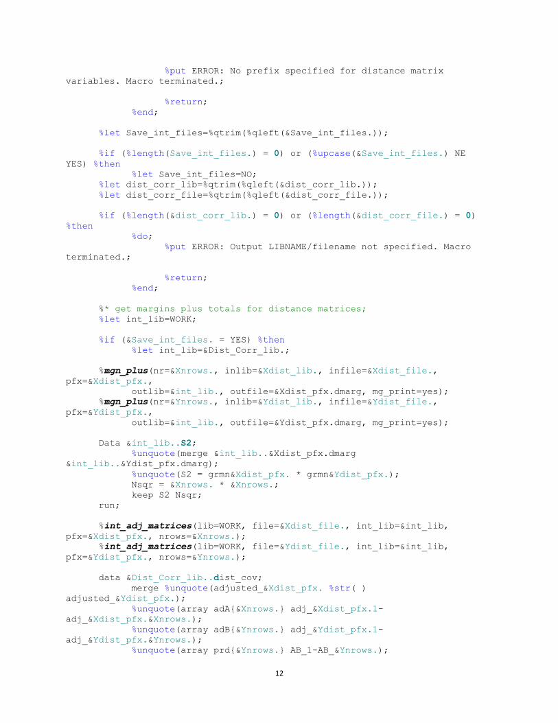
%* get margins plus totals for distance matrices;

%let int_lib=WORK;

%if (&Save_int_files. = YES) %then

%let int_lib=&Dist_Corr_lib.;

%mgn_plus(nr=&Xnrows., inlib=&Xdist_lib., infile=&Xdist_file.,

pfx=&Xdist_pfx.,

outlib=&int_lib., outfile=&Xdist_pfx.dmarg, mg_print=yes);

%mgn_plus(nr=&Ynrows., inlib=&Ydist_lib., infile=&Ydist_file.,

pfx=&Ydist_pfx.,

outlib=&int_lib., outfile=&Ydist_pfx.dmarg, mg_print=yes);

Data &int_lib..S2;

%unquote(merge &int_lib..&Xdist_pfx.dmarg

&int_lib..&Ydist_pfx.dmarg);

%unquote(S2 = grmn&Xdist_pfx. * grmn&Ydist_pfx.);

Nsqr = &Xnrows. * &Xnrows.;

keep S2 Nsqr;

run;

%int_adj_matrices(lib=WORK, file=&Xdist_file., int_lib=&int_lib,

pfx=&Xdist_pfx., nrows=&Xnrows.);

%int_adj_matrices(lib=WORK, file=&Ydist_file., int_lib=&int_lib,

pfx=&Ydist_pfx., nrows=&Ynrows.);

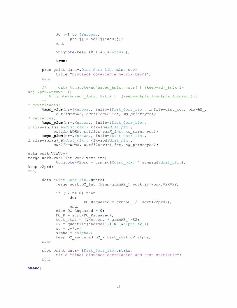
data &Dist_Corr_lib..dist_cov;

merge %unquote(adjusted_&Xdist_pfx. %str( )

adjusted_&Ydist_pfx.);

%unquote(array adA{&Xnrows.} adj_&Xdist_pfx.1-

adj_&Xdist_pfx.&Xnrows.);

%unquote(array adB{&Ynrows.} adj_&Ydist_pfx.1-

adj_&Ydist_pfx.&Ynrows.);

%unquote(array prd{&Ynrows.} AB_1-AB_&Ynrows.);

13

do j=1 to &Ynrows.;

prd{j} = adA{j}*adB{j};

end;

%unquote(keep AB_1-AB_&Ynrows.);

%run;

proc print data=&Dist_Corr_lib..dist_cov;

title "Distance covariance matrix terms";

run;

/* data %unquote(adjusted_&pfx. %str( ) (keep=adj_&pfx.1-

adj_&pfx.&nrows. ))

%unquote(sqradj_&pfx. %str( ) (keep=sq&pfx.1-sq&pfx.&nrows. ));

*/

* covariances;

%mgn_plus(nr=&Xnrows., inlib=&Dist_Corr_lib., infile=dist_cov, pfx=AB_,

outlib=WORK, outfile=DC_int, mg_print=yes);

* variances;

%mgn_plus(nr=&Xnrows., inlib=&Dist_Corr_lib.,

infile=sqradj_&Xdist_pfx., pfx=sq&Xdist_pfx.,

outlib=WORK, outfile=varX_int, mg_print=yes);

%mgn_plus(nr=&Ynrows., inlib=&Dist_Corr_lib.,

infile=sqradj_&Ydist_pfx., pfx=sq&Ydist_pfx.,

outlib=WORK, outfile=varY_int, mg_print=yes);

data work.V2xV2y;

merge work.varX_int work.varY_int;

%unquote(V2prd = grmnsq&Xdist_pfx. * grmnsq&Ydist_pfx.);

keep v2prd;

run;

data &Dist_Corr_lib..stats;

merge work.DC_Int (keep=grmnAB_) work.S2 work.V2XV2Y;

if (S2 ne 0) then

do;

DC_Rsquared = grmnAB_ / (sqrt(V2prd));

end;

else DC_Rsquared = 0;

DC_R = sqrt(DC_Rsquared);

test_stat = (&Xnrows. * grmnAB_)/S2;

CV = quantile('normal',1.0-(&alpha./2));

cv = cv*cv;

alpha = &alpha.;

keep DC_Rsquared DC_R test_stat CV alpha;

run;

proc print data= &Dist_Corr_lib..stats;

title "Final distance correlation and test statistic";

run;

%mend;

14

REFERENCES Note: all URLs quoted or cited herein were accessed in July 2016. Chung, K L, (1974) A Course in Probability Theory. Google Books URL: https://books.google.com/books?id=b2biBQAAQBAJ&printsec=frontcover#v=onepage&q&f=false Clark, M. (2013) A Comparison of Correlation Measures. URL: http://m-clark.github.io/docs/CorrelationComparison.pdf DeGroot, M. (1975) Probability and Statistics. Google Books URL for 2012 updated edition: https://books.google.com/books?id=4TlEPgAACAAJ Ding, AA, Li, Y. (2013) Copula Correlation: An Equitable Dependence Measure and Extension of Pearson's Correlation. In press. URL: http://arxiv.org/pdf/1312.7214 A related paper was presented at the (2016) 19th International Conference on Artificial Intelligence and Statistics; URL: http://jmlr.org/proceedings/papers/v51/chang16.pdf Huo, X et al. (2015) Fast computing for distance covariance. Technometrics. URL: http://arxiv.org/pdf/1410.1503.pdf Kinney JB, Atwal GS. (2014) Equitability, mutual information, and the maximal information coefficient. PNAS. URL: http://www.pnas.org/content/111/9/3354.long Lyons, R. (2013) Distance covariance in metric spaces. The Annals of Probability. URL: http://arxiv.org/pdf/1106.5758.pdf Reshef DN et al. (2011) Detecting novel associations in large data sets. Science, 16 Dec 2011. URL: http://www.ncbi.nlm.nih.gov/pmc/articles/PMC3325791/ Rizzo, ML et al. (2014) Package ‘energy’. URL: http://cran.r-project.org/web/packages/energy/energy.pdf Simon, N & Tibshirani, R. (2011) Comment on" Detecting Novel Associations In Large Data Sets" by Reshef Et Al, Science, Dec 16, 2011. URL: http://arxiv.org/pdf/1401.7645.pdf Speed, T. (2011) A Correlation for the 21

st Century. Science, 16 Dec. 2011. URL:

http://nicorg.pbworks.com/w/file/fetch/50074390/Speed%20Comment%20on%20MIC.pdf (Note: if this URL does not work, check the publisher’s website). Székeley GJ et al. (2007) Measuring and testing dependence by correlation of distances. The Annals of Statistics. URL: http://projecteuclid.org/euclid.aos/1201012979 Székely GJ et al. (2009) Brownian distance covariance. The Annals of Applied Statistics. URL: http://projecteuclid.org/euclid.aoas/1267453933

15

CONTACT INFORMATION: Thomas E. Billings MUFG Union Bank, N.A. Basel II - Retail Credit BTMU 350 California St.; 9th floor MC H-925 San Francisco, CA 94104 Phone: 415-273-2522 Email: tebillings@gmail.com SAS and all other SAS Institute Inc. product or service names are registered trademarks or trademarks of SAS Institute Inc. in the USA and other countries. ® indicates USA registration.

Other brand and product names are trademarks of their respective companies.