distance-based image classification: generalizing to new
TRANSCRIPT
HAL Id: hal-00817211https://hal.inria.fr/hal-00817211
Submitted on 24 Apr 2013
HAL is a multi-disciplinary open accessarchive for the deposit and dissemination of sci-entific research documents, whether they are pub-lished or not. The documents may come fromteaching and research institutions in France orabroad, or from public or private research centers.
L’archive ouverte pluridisciplinaire HAL, estdestinée au dépôt et à la diffusion de documentsscientifiques de niveau recherche, publiés ou non,émanant des établissements d’enseignement et derecherche français ou étrangers, des laboratoirespublics ou privés.
Distance-Based Image Classification: Generalizing tonew classes at near-zero cost
Thomas Mensink, Jakob Verbeek, Florent Perronnin, Gabriela Csurka
To cite this version:Thomas Mensink, Jakob Verbeek, Florent Perronnin, Gabriela Csurka. Distance-Based Image Clas-sification: Generalizing to new classes at near-zero cost. IEEE Transactions on Pattern Analysis andMachine Intelligence, Institute of Electrical and Electronics Engineers, 2013, 35 (11), pp.2624-2637.�10.1109/TPAMI.2013.83�. �hal-00817211�

IEEE TRANSACTIONS ON PATTERN RECOGNITION AND MACHINE INTELLIGENCE 1
Distance-Based Image Classification:Generalizing to new classes at near-zero cost
Thomas Mensink, Member IEEE, Jakob Verbeek, Member, IEEE,Florent Perronnin, and Gabriela Csurka
Abstract—We study large-scale image classification methods that can incorporate new classes and training images continuouslyover time at negligible cost. To this end we consider two distance-based classifiers, the k-nearest neighbor (k-NN) and nearestclass mean (NCM) classifiers, and introduce a new metric learning approach for the latter. We also introduce an extension of theNCM classifier to allow for richer class representations. Experiments on the ImageNet 2010 challenge dataset, which containsover 106 training images of 1,000 classes, show that, surprisingly, the NCM classifier compares favorably to the more flexiblek-NN classifier. Moreover, the NCM performance is comparable to that of linear SVMs which obtain current state-of-the-artperformance. Experimentally we study the generalization performance to classes that were not used to learn the metrics. Usinga metric learned on 1,000 classes, we show results for the ImageNet-10K dataset which contains 10,000 classes, and obtainperformance that is competitive with the current state-of-the-art, while being orders of magnitude faster. Furthermore, we showhow a zero-shot class prior based on the ImageNet hierarchy can improve performance when few training images are available.
Index Terms—Metric Learning, k-Nearest Neighbors Classification, Nearest Class Mean Classification, Large Scale ImageClassification, Transfer Learning, Zero-Shot Learning, Image Retrieval
F
1 INTRODUCTION
I N this paper we focus on the problem of large-scale, multi-class image classification, where the goal is to assign
automatically an image to one class out of a finite set ofalternatives, e.g . the name of the main object appearing inthe image, or a general label like the scene type of theimage. To ensure scalability, often linear classifiers suchas linear SVMs are used [1], [2]. Additionally, to speed-up classification, dimension reduction techniques could beused [3], or a hierarchy of classifiers could be learned [4],[5]. The introduction of the ImageNet dataset [6], whichcontains more than 14M manually labeled images of 22Kclasses, has provided an important benchmark for large-scaleimage classification and annotation algorithms. Recently,impressive results have been reported on 10,000 or moreclasses [1], [3], [7]. A drawback of these methods, however,is that when images of new categories become available, newclassifiers have to be trained from scratch at a relatively highcomputational cost.
Many real-life large-scale datasets are open-ended anddynamic: new images are continuously added to existingclasses, new classes appear over time, and the semanticsof existing classes might evolve too. Therefore, we are
• Thomas MensinkISLA Lab - University of AmsterdamE-mail: [email protected]
• Jakob VerbeekLEAR Team - INRIA GrenobleE-mail: [email protected]
• Florent Perronnin and Gabriela CsurkaXerox Research Centre EuropeE-mail: [email protected]
interested in distance-based classifiers which enable theaddition of new classes and new images to existing classesat (near) zero cost. Such methods can be used continuouslyas new data becomes available, and additionally alternatedfrom time to time with a computationally heavier methodto learn a good metric using all available training data. Inparticular we consider two distance-based classifiers.
The first is the k-nearest neighbor (k-NN) classifier, whichuses all examples to represent a class, and is a highly non-linear classifier that has shown competitive performance forimage classification [3], [7], [8], [9]. New images (of newclasses) are simply added to the database, and can be usedfor classification without further processing.
The second is the nearest class mean classifier (NCM),which represents classes by their mean feature vector of itselements, see e.g . [10]. Contrary to the k-NN classifier, thisis an efficient linear classifier. To incorporate new images (ofnew classes), the relevant class means have to be adjusted oradded to the set of class means. In Section 3, we introducean extension which uses several prototypes per class, whichallows a trade-off between the model complexity and thecomputational cost of classification.
The success of these methods critically depends on theused distance functions. Therefore, we cast our classifierlearning problem as one of learning a low-rank Mahalanobisdistance which is shared across all classes. The dimension-ality of the low-rank matrix is used as regularizer, and toimprove computational and storage efficiency.
In this paper we explore several strategies for learningsuch a metric. For the NCM classifier, we propose a novelmetric learning algorithm based on multi-class logistic dis-crimination (NCMML), where a sample from a class isenforced to be closer to its class mean than to any other
IEEE TRANSACTIONS ON PATTERN RECOGNITION AND MACHINE INTELLIGENCE 2
class mean in the projected space. We show qualitatively andquantitatively the advantages of our NCMML approach overthe classical Fisher Discriminant Analysis [10]. For k-NNclassification, we rely on the Large Margin Nearest Neighbor(LMNN) framework [11] and investigate two variationssimilar to the ideas presented in [11], [12] that significantlyimprove classification performance.
Most of our experiments are conducted on the Im-ageNet Large Scale Visual Recognition Challenge 2010(ILSVRC’10) dataset, which consists of 1.2M training im-ages of 1,000 classes. To apply the proposed metric learn-ing techniques on such a large-scale dataset, we employstochastic gradient descend (SGD) algorithms, which accessonly a small fraction of the training data at each iteration[13]. To allow metric learning on high-dimensional imagefeatures of datasets that are too large to fit in memory, weuse in addition product quantization [14], a data compressiontechnique that was recently used with success for large-scaleimage retrieval [15] and classifier training [1].
As a baseline approach, we follow the winning entry ofthe ILSVRC’11 challenge [1]: Fisher vector image repre-sentations [16] are used to describe images and one-vs-rest linear SVM classifiers are learned independently foreach class. Surprisingly, we find that the NCM classifieroutperforms the more flexible k-NN classifier. Moreover, theNCM classifier performs on par with the SVM baseline, andshows competitive performance on new classes.
This paper extends our earlier work [17], as follows.First, for the NCM classifier, in Section 3, we compare theNCMML metric learning to the classic FDA, we introducean extension which uses multiple centroids per class, weexplore a different learning objective, and we examine thecritical points of the objective. Second, in Section 4, weprovide more details on the SGD triplet sampling strategyused for LMNN metric learning, and we present an efficientgradient evaluation method. Third, we extend the experimen-tal evaluation with an experiment where NCMML is usedto learn a metric for instance level image retrieval.
The rest of the paper is organized as follows. We firstdiscuss a selection of related works which are most relevantto this paper. In Section 3 we introduce the NCM classifierand the NCMML metric learning approach. In Section 4we review LMNN metric learning for k-NN classifiers.We present extensive experimental results in Section 5,analyzing different aspects of the proposed methods andcomparing them to the current state-of-the-art in differentapplication settings such as large scale image annotation,transfer learning and image retrieval. Finally, we present ourconclusions in Section 6.
2 RELATED WORK
In this section we review related work on large-scale imageclassification, metric learning, and transfer learning.
2.1 Large-scale image classificationThe ImageNet dataset [6] has been a catalyst for researchon large-scale image annotation. The current state-of-the-art
[1], [2] uses efficient linear SVM classifiers trained in a one-vs-rest manner in combination with high-dimensional bag-of-words [18], [19] or Fisher vector representations [16].Besides one-vs-rest training, large-scale ranking-based for-mulations have also been explored in [3]. Interestingly, theirWSABIE approach performs joint classifier learning anddimensionality reduction of the image features. Operatingin a lower-dimensional space acts as a regularization duringlearning, and also reduces the cost of classifier evaluationat test time. Our proposed NCM approach also learns low-dimensional projection matrices but the weight vectors areconstrained to be the projected class means. This allows forefficient addition of novel classes.
In [3], [7] k-NN classifiers were found to be competitivewith linear SVM classifiers in a very large-scale settinginvolving 10,000 or more classes. The drawback of k-NNclassifiers, however, is that they are expensive in storageand computation, since in principle all training data needsto be kept in memory and accessed to classify new images.This holds even more for Naive-Bayes Nearest Neighbor(NBNN) [9], which does not use descriptor quantization, butrequires storage of all local descriptors of all training images.The storage issue is also encountered when SVM classifiersare trained since all training data needs to be processed inmultiple passes. Product quantization (PQ) was introducedin [15] as a lossy compression mechanism for local SIFTdescriptors in a bag-of-features image retrieval system. Ithas been subsequently used to compress bag-of-words andFisher vector image representations in the context of imageretrieval [20] and classifier training [1]. We also exploit PQencoding in our work to compress high-dimensional imagesignatures when learning our metrics.
2.2 Metric learning
There is a large body of literature on metric learning, buthere we limit ourselves to highlighting just several methodsthat learn metrics for (image) classification problems. Othermethods aim at learning metrics for verification problemsand essentially learn binary classifiers that threshold thelearned distance to decide whether two images belong tothe same class or not, see e.g . [21], [22], [23]. Yet anotherline of work concerns metric learning for ranking problems,e.g . to address text retrieval tasks as in [24].
Among those methods that learn metrics for classification,the Large Margin Nearest Neighbor (LMNN) approach of[11] is specifically designed to support k-NN classification.It tries to ensure that for each image a predefined set oftarget neighbors from the same class are closer than samplesfrom other classes. Since the cost function is defined overtriplets of points —that can be sampled in an SGD trainingprocedure— this method can scale to large datasets. The setof target neighbors is chosen and fixed using the `2 metric inthe original space; this can be problematic as the `2 distancemight be quite different from the optimal metric for imageclassification. Therefore, we explore two variants of LMNNthat avoid using such a pre-defined set of target neighbors,similar to the ideas presented in [12].

IEEE TRANSACTIONS ON PATTERN RECOGNITION AND MACHINE INTELLIGENCE 3
The large margin nearest local mean classifier [25] assignsa test image to a class based on the distance to the mean of itsnearest neighbors in each class. This method was reportedto outperform LMNN but requires computing all pairwisedistances between training instances and therefore does notscale well to large datasets. Similarly, TagProp [8] suffersfrom the same problem; it consists in assigning weights totraining samples based on their distance to the test instanceand in computing the class prediction by the total weight ofsamples of each class in a neighborhood.
Other closely related methods are metric learning by col-lapsing classes [26] and neighborhood component analysis[27]. As TagProp, for each data point these define weightsto other data points proportional to the exponent of negativedistance. In [26] the target is to learn a distance that makesthe weights uniform for samples of the same class andclose to zero for other samples. While in [27] the targetis only to ensure that zero weight is assigned to samplesfrom other classes. These methods also require computingdistances between all pairs of data points. Because of theirpoor scaling, we do not consider any of these methods below.
Closely related to our NCMML metric learning approachfor the NCM classifier is the LESS model of [28]. Theylearn a diagonal scaling matrix to modify the `2 distance byrescaling the data dimensions, and include an `1 penalty onthe weights to perform feature selection. However, in theircase, NCM is used to address small sample size problemsin binary classification, i.e . cases where there are fewertraining points (tens to hundreds) than features (thousands).Our approach differs significantly in that (i) we work ina multi-class setting and (ii) we learn a low-dimensionalprojection which allows efficiency in large-scale.
Another closely related method is the Taxonomy-embedding method of [29], where a nearest prototype classi-fier is used in combination with a hierarchical cost function.Documents are embedded in a lower dimensional space inwhich each class is represented by a single prototype. Incontrast to our approach, they use a predefined embeddingof the images and learn low-dimensional classifies, andtherefore their method resembles more to the WSABIEmethod of [3].
The Sift-bag kernel of [30] is also related to our methodsince it uses an NCM classifier and an `2 distance in asubspace that is orthogonal to the subspace with maximumwithin-class variance. However, it involves computing thefirst eigenvectors of the within-class covariance matrix,which has a computational cost betweenO(D2) andO(D3),undesirable for high-dimensional feature vectors. Moreover,this metric is heuristically obtained, rather than directlyoptimized for maximum classification performance.
Finally, the image-to-class metric learning method of [31],learns per class a Mahalanobis metric, which in contrast toour method cannot generalize to new classes. Besides, it usesthe idea of NBNN [9], and therefore requires the storage ofall local descriptors of all images, which is impractical forthe large-scale datasets used in this paper.
2.3 Transfer learning
The term transfer learning is used to refer to methods thatshare information across classes during learning. Examplesof transfer learning in computer vision include the useof part-based or attribute class representations. Part-basedobject recognition models [32] define an object as a spatialconstellation of parts, and share the part detectors acrossdifferent classes. Attribute-based models [33] characterizea category (e.g . a certain animal) by a combination ofattributes (e.g . is yellow, has stripes, is carnivore), and sharethe attribute classifiers across classes. Other approachesinclude biasing the weight vector learned for a new classtowards the weight vectors of classes that have already beentrained [34]. Zero-shot learning [35] is an extreme case oftransfer learning where for a new class no training instancesare available but a description is provided in terms ofparts, attributes, or other relations to already learned classes.Transfer learning is related to multi-task learning, wherethe goal is to leverage the commonalities between severaldistinct but related classification problems, or classifierslearned for one type of images (e.g . ImageNet) are adapted toa new domain (e.g . imagery obtained from a robot camera),see e.g . [36], [37].
In [38] various transfer learning methods were evalu-ated in a large-scale setting using the ILSVRC’10 dataset.They found transfer learning methods to have little addedvalue when training images are available for all classes.In contrast, transfer learning was found to be effective ina zero-shot learning setting, where classifiers were trainedfor 800 classes, and performance was tested in a 200-wayclassification across the held-out classes.
In this paper we also aim at transfer learning, in the sensethat we allow only a trivial amount of processing on thedata of new classes (storing in a database, or averaging),and rely on a metric that was trained on other classes torecognize the new ones. In contrast to most works on transferlearning, we do not use any intermediate representation interms of parts or attributes, nor do we train classifiers forthe new classes. While also considering zero-shot learning,we further evaluate performance when combining a zero-shot model inspired by [38] with progressively more trainingimages per class, from one up to thousands. We find that thezero-shot model provides an effective prior when a smallamount of training data is available.
3 THE NEAREST CLASS MEAN CLASSIFIER
The nearest class mean (NCM) classifier assigns an imageto the class c∗ ∈ {1, . . . , C} with the closest mean:
c∗ = argminc∈{1,...,C}
d(x,µc), (1)
µc =1
Nc
∑i:yi=c
xi, (2)
where d(x,µc) is the Euclidean distance between an imagex and the class mean µc, and yi is the ground-truth label ofimage i, and Nc is the number of training images in class c.

IEEE TRANSACTIONS ON PATTERN RECOGNITION AND MACHINE INTELLIGENCE 4
Next, we introduce our NCM metric learning approach,and its relations to existing models. Then, we present an ex-tension to use multiple centroids per class, which transformsthe NCM into a non-linear classifier. Finally, we exploresome variants of the objective which allow for smaller SGDbatch sizes, and we give some insights in the critical pointsof the objective function.
3.1 Metric learning for the NCM classifierIn this section we introduce our metric learning approach,which we will refer to as “nearest class mean metric learn-ing” (NCMML). We replace the Euclidean distance in NCMby a learned (squared) Mahalanobis distance:
dM (x,x′) = (x− x′)>M(x− x′), (3)
where x and x′ are D dimensional vectors, and M isa positive definite matrix. We focus on low-rank metricswith M = W>W and W ∈ IRd×D, where d ≤ Dacts as regularizer and improves efficiency for computationand storage. The Mahalanobis distance induced by W isequivalent to the squared `2 distance after linear projectionof the feature vectors on the rows of W :
dW (x,x′) = (x− x′)>W>W (x− x′)= ‖Wx−Wx′ ‖22 . (4)
We do not consider using the more general formulationof M = W>W + S, where S is a diagonal matrix, asin [24]. While this formulation requires only D additionalparameters to estimate, it still requires computing distancesin the original high-dimensional space. This is costly forthe dense and high-dimensional (4K-64K) Fisher vectorsrepresentations we use in our experiments, see Section 5.
We formulate the NCM classifier using a probabilisticmodel based on multi-class logistic regression and definethe probability for a class c given an feature vector x as:
p(c|x) =exp
(− 1
2dW (x,µc))∑C
c′=1 exp(− 1
2dW (x,µc′)) . (5)
This definition may also be interpreted as giving the pos-terior probabilities of a generative model where p(xi|c) =N (xi;µc,Σ), is a Gaussian with meanµc, and a covariancematrix Σ =
(W>W
)−1, which is shared across all classes1.
The class probabilities p(c) are set to be uniform over allclasses. Later, in Eq. (21), we formulate an NCM classifierwith non-uniform class probabilities.
To learn the projection matrix W , we maximize the log-likelihood of the correct predictions of the training images:
L =1
N
N∑i=1
ln p(yi|xi). (6)
The gradient of the NCMML objective Eq. (6) is:
∇WL =1
N
N∑i=1
C∑c=1
αic W zicz>ic, (7)
1. Strictly speaking the covariance matrix is not properly defined as thelow-rank matrix W>W is non-invertible.
Fig. 1: Illustration to compare FDA (left) and NCMML(right), the obtained projection direction is indicated by thegray line on which also the projected samples are plotted.For FDA the result is clearly suboptimal since the blueand green classes are collapsed in the projected space.The proposed NCMML method finds a projection directionwhich separates the classes reasonably well.
where αic = p(c|xi)− [[yi = c]], zic = µc−xi, and we usethe Iverson brackets [[·]] to denote the indicator function thatequals one if its argument is true and zero otherwise.
Although not included above for clarity, the terms inthe log-likelihood in Eq. (6) could be weighted in caseswhere the class distributions in the training data are notrepresentative for those when the learned model is applied.
3.2 Relation to existing linear classifiers
First we compare the NCMML objective with the classicFisher Discriminant Analysis (FDA) [10]. The objective ofFDA is to find a projection matrix W that maximizes theratio of between-class variance to within-class variance:
LFDA = tr
(WSBW
>
WSWW>
), (8)
where SB =∑C
c=1Nc
N (µ − µc)(µ − µc)> is the weighted
covariance matrix of the class centers (µ being the datacenter), and SW =
∑Cc=1
Nc
N Σc is the weighted sum ofwithin class covariance matrices Σc, see e.g . [10] for details.
In the case where the within class covariance for eachclass equals the identity matrix, the FDA objective seeksthe direction of maximum variance in SB, i.e . it performsa PCA projection on the class means. To illustrate this, weshow an example of a two-dimensional problem with threeclasses in Figure 1. In contrast, our NCMML method aimsat separating the classes which are nearby in the projectedspace, so as to ensure correct predictions. The resultingprojection separates the three classes reasonably well.
To relate the NCM classifier to other linear classifiers, werepresent them using the class specific score functions:
f(c,x) = w>c x+ bc, (9)
which are used to assign samples to the class with maximumscore. NCM can be recognized as a linear classifier by

IEEE TRANSACTIONS ON PATTERN RECOGNITION AND MACHINE INTELLIGENCE 5
defining fNCM with bias and weight vectors given by:
bc = − 12 ‖Wµc ‖22, (10)
wc = W>Wµc. (11)
This is because − 12dW (x,µc) in Eq. (5) can be written as:
− 12‖Wx‖
22 − 1
2‖Wµc ‖22 + x>W>Wµc,
where the first term is independent of the class c andtherefore irrelevant for classification.
These definitions allows us to relate the NCM classifierto other linear methods. For example, we obtain standardmulti-class logistic regression, if the restrictions on bc andwc are removed. Note that these are precisely the restrictionsthat allow us adding new classes at near-zero cost, since theclass specific parameters bc and wc are defined by just theclass means µc and the class-independent projection W .
In WSABIE [3] fWSABIE is defined using bc = 0 and,
wc = W>vc, (12)
where W ∈ IRd×D is also a low-rank projection matrixshared between all classes, and vc is a class specific weightvector of dimensionality d, both learned from data. This issimilar to NCM if we set vc = Wµc. As in multiclasslogistic regression, however, for WSABIE the vc need to belearned from scratch for new classes.
The NCM classifier can also be related to the solutionof ridge-regression (RR, or regularized linear least-squaresregression), where the parameters bc and wc are learned byoptimizing the squared loss:
LRR =1
N
∑i
(fRR(c,xi)− yic
)2+ λ ‖wc ‖22, (13)
where λ acts as regularizer, and where yic = 1, if image ibelongs to class c, and yic = 0 otherwise. The loss LRR canbe minimized in closed form and leads to:
bc =Nc
N, and wc =
Nc
Nµ>c (Σ + λI)−1, (14)
where Σ is the (class-independent) data covariance matrix.Just like the NCM classifier, the RR classifier also allowsto add new classes at low cost, since the class specificparameters can be found from the class means and countsonce the data covariance matrix Σ has been estimated.Moreover, if Nc is equal for all classes, RR is similar toNCM with W set such that W>W = (Σ + λI)−1.
Finally, the Taxonomy-embedding [29] scores a class by:
fTAX(c,x) = v>c W>Wx− 1
2 ‖vc ‖22, (15)
where W ∈ IRC×D projects the data to a C dimensionalspace, and is set using a closed-form solution based onridge-regression. The class-specific weight vectors vc arelearned from the data. Therefore, this method relates to theWSABIE method; it learns the classifier in low-dimensionalspace (if C < D), but in this case the projection matrix Wis given in closed-form. It also shares the disadvantage ofthe WSABIE method: it cannot generalize to novel classeswithout retraining.
3.3 Non-linear NCM with multiple class centroids
In this section we extend the NCM classifier to allow formore flexible class representations, which result in non-linear classification. The idea is to represent each class by aset of centroids, instead of only the class mean.
Assume that we have a set of k centroids {mcj}kj=1 foreach class c. The posterior probability for class c can bedefined as:
p(c|x) =
k∑j=1
p(mcj |x), (16)
p(mcj |x) =1
Zexp
(− 1
2dW (x,mcj)), (17)
where p(mcj |x) denotes the posterior of a centroid mcj ,and Z =
∑c
∑j exp
(− 1
2dW (x,mcj))
is the normalizer.The value k offers a transition between NCM (k = 1),
and a weighted k-NN (k equals all images per class), wherethe weight of each neighbor is defined by the soft-min of itsdistance, c.f . Eq. (17). This is similar to TagProp [8], usedfor multi-label image annotation.
This model also corresponds to a generative model, wherethe probability for a feature vectorx, to be generated by classc, is given by a Gaussian mixture distribution:
p(x|c) =
k∑j=1
πcj N (xi;mcj ,Σ) , (18)
with equal mixing weights πcj = 1/k, and the covariancematrix Σ shared among all classes. We refer to this methodas the nearest class multiple centroids (NCMC) classifier.A similar model was independently developed recently forimage retrieval in [39]. Their objective, however, is todiscriminate between different senses of a textual query, andthey use a latent model to select the sense of a query.
To learn the projection matrix W , we again maximizethe log-likelihood of correct classification, for which thegradient w.r.t. W in this case is given by:
∇WL =1
N
∑i,c,j
αicj W zicjz>icj , (19)
where zicj = mcj − xi, and
αicj = p(mcj |xi)− [[c = yi]]p(mcj |xi)∑j′ p(mcj′ |xi)
. (20)
To obtain the centroids of each class, we apply k-meansclustering on the features x belonging to that class, usingthe `2 distance. Instead of using a fixed set of class means, itcould be advantageous to iterate the k-means clustering andthe learning of the projection matrix W . Such a strategy al-lows the set of class centroids to represent more precisely thedistribution of the images in the projected space, and mightfurther improve the classification performance. However theexperimental validation of such a strategy falls beyond thescope of this paper.
IEEE TRANSACTIONS ON PATTERN RECOGNITION AND MACHINE INTELLIGENCE 6
TABLE 1: Comparison of complexity of the consideredalternatives to compute the class probabilities p(c|x).
Distances in D dimensions O(dD(mC) +mC(d+D)
)Distances in d dimensions O
(dD(m+ C) +mC(d)
)Dot product formulation O
(dD(m) +mC(D)
)
3.4 Alternative objective for small SGD batches
Computing the gradients for NCMML in Eq. (7) and NCMCin Eq. (19) is relatively expensive, regardless of the numberof m samples used per SGD iteration. The cost of thiscomputation is dominated by the computation of the squareddistances dW (x,µc), required to compute the m × Cprobabilities p(c|x) for C classes in the SGD update. Tocompute these distances we have two options. First, wecan compute the m × C difference vectors (x − µc),project these on the d × D matrix W , and compute thenorms of the projected difference vectors, at a total cost ofO(dD(mC) + mC(d + D)
). Second, we can first project
both the m data vectors and C class centers, and thencompute distances in the low dimensional space, at a totalcost of O
(dD(m+C)+mC(d)
). Note that the latter option
has a lower complexity, but still requires projecting all classcenters at a costO(dDC), which will be the dominating costwhen using small SGD batches with m � C. Therefore,in practice we are limited to using SGD batch sizes withm ≈ C = 1, 000 samples.
In order to accommodate for fast SGD updates based onsmaller batch sizes, we replace the Euclidean distance inEq. (5) by the negative dot-product plus a class specific biassc. The probability for class c is now given by:
p(c|xi) =1
Zexp
(x>i W
>Wµc + sc
), (21)
where Z denotes the normalizer. The objective is stillto maximize the log-likelihood of Eq. (6). The efficiencygain stems from the fact that we can avoid projecting theclass centers on W , by twice projecting the data vectors:xi = x>i W
>W , and then computing dot-products in highdimensional space 〈xi,µc〉. For a batch of m images, thefirst step costs O(mDd), and the latter O(mCD), resultingin a complexity of O
(dD(m) +mC(D)
). This complexity
scales linearly with m, and is lower for small batches withm ≤ d, since in that case it is more costly to project the classvectors on W than on the double-projected data vectors xi.For clarity, we summarize the complexity of the differentalternatives we considered in Table 1.
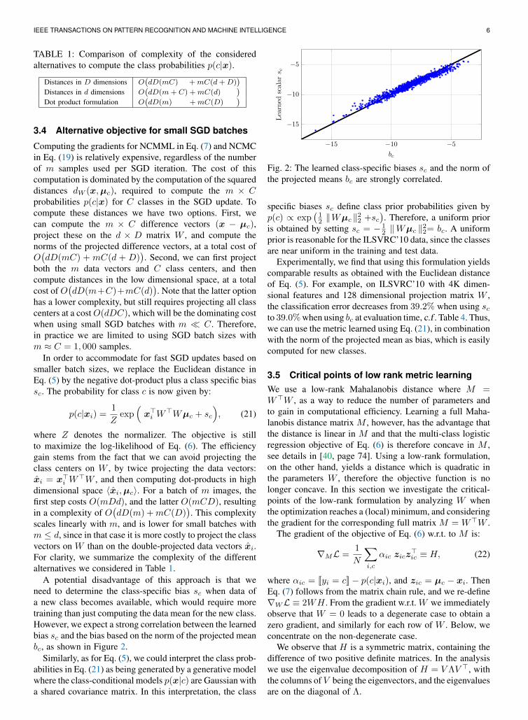
A potential disadvantage of this approach is that weneed to determine the class-specific bias sc when data ofa new class becomes available, which would require moretraining than just computing the data mean for the new class.However, we expect a strong correlation between the learnedbias sc and the bias based on the norm of the projected meanbc, as shown in Figure 2.
Similarly, as for Eq. (5), we could interpret the class prob-abilities in Eq. (21) as being generated by a generative modelwhere the class-conditional models p(x|c) are Gaussian witha shared covariance matrix. In this interpretation, the class
−15 −10 −5
−15
−10
−5
bc
Learned
scalar
s c
Fig. 2: The learned class-specific biases sc and the norm ofthe projected means bc are strongly correlated.
specific biases sc define class prior probabilities given byp(c) ∝ exp
(12 ‖Wµc ‖22 +sc
). Therefore, a uniform prior
is obtained by setting sc = − 12 ‖Wµc ‖22= bc. A uniform
prior is reasonable for the ILSVRC’10 data, since the classesare near uniform in the training and test data.
Experimentally, we find that using this formulation yieldscomparable results as obtained with the Euclidean distanceof Eq. (5). For example, on ILSVRC’10 with 4K dimen-sional features and 128 dimensional projection matrix W ,the classification error decreases from 39.2% when using scto 39.0% when using bc at evaluation time, c.f . Table 4. Thus,we can use the metric learned using Eq. (21), in combinationwith the norm of the projected mean as bias, which is easilycomputed for new classes.
3.5 Critical points of low rank metric learningWe use a low-rank Mahalanobis distance where M =W>W , as a way to reduce the number of parameters andto gain in computational efficiency. Learning a full Maha-lanobis distance matrix M , however, has the advantage thatthe distance is linear in M and that the multi-class logisticregression objective of Eq. (6) is therefore concave in M ,see details in [40, page 74]. Using a low-rank formulation,on the other hand, yields a distance which is quadratic inthe parameters W , therefore the objective function is nolonger concave. In this section we investigate the critical-points of the low-rank formulation by analyzing W whenthe optimization reaches a (local) minimum, and consideringthe gradient for the corresponding full matrix M = W>W .
The gradient of the objective of Eq. (6) w.r.t. to M is:
∇ML =1
N
∑i,c
αic zicz>ic ≡ H, (22)
where αic = [[yi = c]]− p(c|xi), and zic = µc − xi. ThenEq. (7) follows from the matrix chain rule, and we re-define∇WL ≡ 2WH . From the gradient w.r.t. W we immediatelyobserve that W = 0 leads to a degenerate case to obtain azero gradient, and similarly for each row of W . Below, weconcentrate on the non-degenerate case.
We observe that H is a symmetric matrix, containing thedifference of two positive definite matrices. In the analysiswe use the eigenvalue decomposition of H = V ΛV >, withthe columns of V being the eigenvectors, and the eigenvaluesare on the diagonal of Λ.
IEEE TRANSACTIONS ON PATTERN RECOGNITION AND MACHINE INTELLIGENCE 7
We can now express the gradient for W as
∇WL = 2WV ΛV > ≡ G. (23)
Thus the gradient of the i-th row of W , which we denoteby gi, is a linear combination of the eigenvectors of H:
gi ≡∑j
λj〈wi,vj〉vj , (24)
where wi and vj denote the i-th row of W and the j-thcolumn of V respectively. Thus an SGD gradient updatewill drive a row of W towards the eigenvectors of H that (i)have a large positive eigenvalue, and (ii) are most alignedwith that row of W . This is intuitive, since we would expectthe low-rank formulation to focus on the most significantdirections of the full-rank metric.
Moreover, the expression for the gradient in Eq. (24)shows that at a critical pointW ∗ of the objective function, alllinear combination coefficients are zero: ∀i,j : λj〈w∗i ,vj〉 =0. This indicates that at the critical point, for each row w∗iand each eigenvector vj it holds that eitherw∗i is orthogonalto vj , or that vj has a zero associated eigenvalue, i.e . λj = 0.Thus, at a critical point W ∗, the corresponding gradient forthe full rank formulation at that point, withM∗ = W ∗>W ∗,is zero in the subspace spanned by W ∗.
Given this analysis, we believe it is unlikely to attainpoor local minima using the low rank formulation. Indeed,the gradient updates for W are aligned with the mostimportant directions of the corresponding full-rank gradient,and at convergence the full-rank gradient is zero in thesubspace spanned by W . To confirm this, we have alsoexperimentally investigated this by training several timeswith different random initializations of W . We observe thatthe classification performance differs at most ±0.1% on anyof the error measures used in Section 5, and that the numberof SGD iterations selected by the early stopping procedureare of the same order.
4 K-NN METRIC LEARNINGWe compare the NCM classifier to the k-NN classifier,a frequently used distance based classifier. For successfulk-NN classification, the majority of the nearest neighborsshould be of the same class. This is reflected in the LMNNmetric learning objective [11], which is defined over tripletsconsisting of a query image q, an image p from the sameclass, and an image n from another class:
Lqpn =[1 + dW (xq,xp)− dW (xq,xn)
]+, (25)
where [z]+ = max(0, z). The hinge-loss for a triplet is zeroif the negative image n is at least one distance unit fartherfrom the query q than the positive image p, and the lossis positive otherwise. The final learning objective sums thelosses over all triplets:
LLMNN =∑q
∑p∈Pq
∑n∈Nq
Lqpn, (26)
where Pq and Nq denote a predefined set of positive andnegative images for each query image q. Also in this casewe could weight the terms in the loss function to accountfor non-representative class proportions in the training data.
Choice of target neighbors.In the basic version of LMNN the set of targets Pq for aquery q is set to the query’s k nearest neighbors from thesame class, using the `2 distance. The rationale is that ifwe ensure that these targets are closer than the instances ofthe other classes, then the k-NN classification will succeed.However, this implicitly assumes that the `2-targets will alsobe the closest points from the same class using the learnedmetric, which in practice might not be the case. Therefore,we consider two alternatives to using a fixed set of targetneighbors.
First, we consider Pq to contain all images of the sameclass as q, hence the selection is independent on the metric.This is similar to [12] where the same type of loss was used tolearn image similarity defined as the scalar product betweenfeature vectors after a learned linear projection.
Second, we consider dynamically updating Pq to containthe k images of the same class that are closest to q using thecurrent metricW , hence different target neighbors can be se-lected depending on the metric. This method corresponds tominimizing the loss function also with respect to the choiceof Pq . A similar approach was proposed in [11], where everyT iterations Pq is redefined using target neighbors accordingto the current metric.
Triplet sampling strategy.Here, we describe a sampling strategy which obtains themaximal number of triplets from m images selected perSGD iteration. Using a small m is advantageous since thecost of the gradient evaluation is in large part determined bycomputing the projections Wx of the images, and, if used,the cost of decompressing the PQ encoded signatures.
To generate triplets, we first select uniformly at randoma class c that will provide the query and positive images.When Pq is set to contain all images of the same class, wesample 2
3m images from the class c, and 13m images across
other classes. In this manner we can construct about 427m
3
triplets, i.e . about 4 million triplets for m = 300 used in ourexperiments, see our technical report [41] for more details.
For other choices of Pq we do the following:• For a fixed set of target neighbors, we still sample
13m negative images, and take as many query imagestogether with their target neighbors until we obtain 2
3mimages allocated for the positive class.
• For a dynamic set of target neighbors we simplyselect the closest neighbors among the 2
3m sampledpositive images using the current metric W . Althoughapproximate, this avoids computing the dynamic targetneighbors among all the images in the positive class.
Efficient gradient evaluation.For either choice of the target set Pq , the gradient can becomputed without explicitly iterating over all triplets, bysorting the distances w.r.t. query images. The sub-gradientof the loss of a triplet is given by:
∇WLqpn = [[Lqpn > 0]] 2 W(xqpx
>qp − xqnx
>qn
), (27)
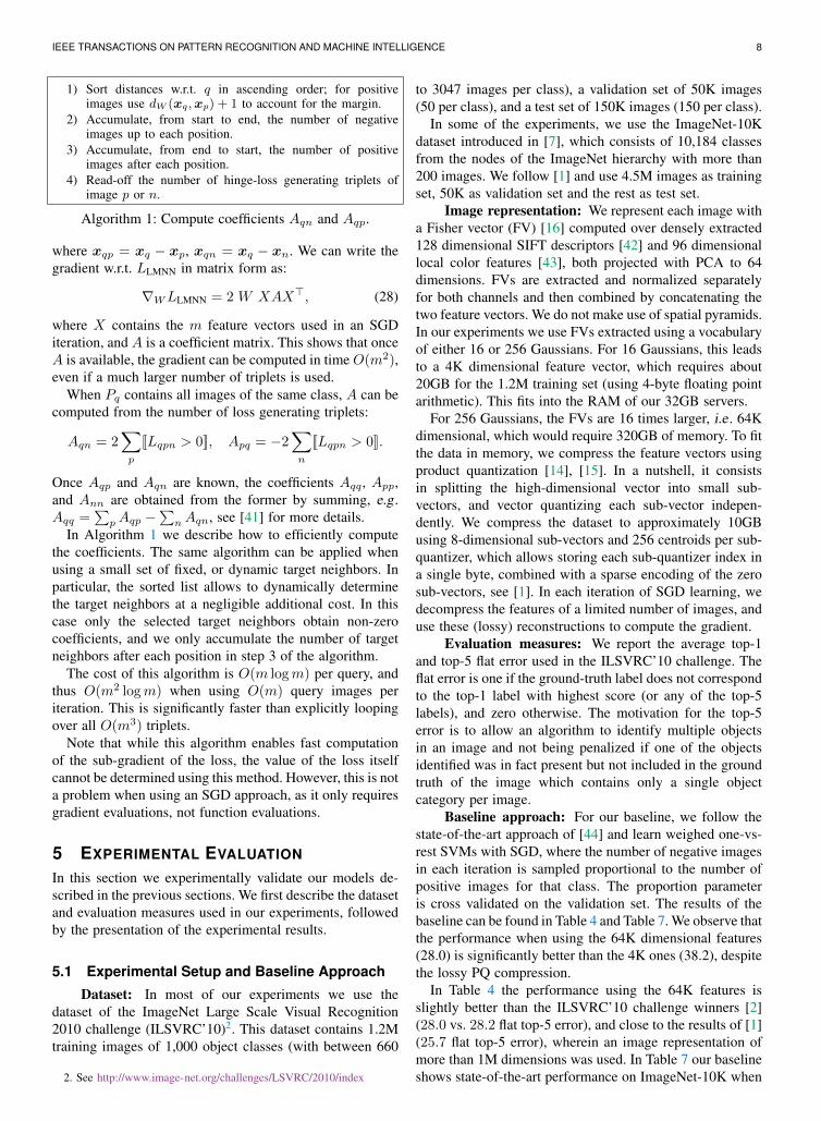
IEEE TRANSACTIONS ON PATTERN RECOGNITION AND MACHINE INTELLIGENCE 8
1) Sort distances w.r.t. q in ascending order; for positiveimages use dW (xq,xp) + 1 to account for the margin.
2) Accumulate, from start to end, the number of negativeimages up to each position.
3) Accumulate, from end to start, the number of positiveimages after each position.
4) Read-off the number of hinge-loss generating triplets ofimage p or n.
Algorithm 1: Compute coefficients Aqn and Aqp.
where xqp = xq − xp, xqn = xq − xn. We can write thegradient w.r.t. LLMNN in matrix form as:
∇WLLMNN = 2 W XAX>, (28)
where X contains the m feature vectors used in an SGDiteration, and A is a coefficient matrix. This shows that onceA is available, the gradient can be computed in time O(m2),even if a much larger number of triplets is used.
When Pq contains all images of the same class, A can becomputed from the number of loss generating triplets:
Aqn = 2∑p
[[Lqpn > 0]], Apq = −2∑n
[[Lqpn > 0]].
Once Aqp and Aqn are known, the coefficients Aqq , App,and Ann are obtained from the former by summing, e.g .Aqq =
∑pAqp −
∑nAqn, see [41] for more details.
In Algorithm 1 we describe how to efficiently computethe coefficients. The same algorithm can be applied whenusing a small set of fixed, or dynamic target neighbors. Inparticular, the sorted list allows to dynamically determinethe target neighbors at a negligible additional cost. In thiscase only the selected target neighbors obtain non-zerocoefficients, and we only accumulate the number of targetneighbors after each position in step 3 of the algorithm.
The cost of this algorithm is O(m logm) per query, andthus O(m2 logm) when using O(m) query images periteration. This is significantly faster than explicitly loopingover all O(m3) triplets.
Note that while this algorithm enables fast computationof the sub-gradient of the loss, the value of the loss itselfcannot be determined using this method. However, this is nota problem when using an SGD approach, as it only requiresgradient evaluations, not function evaluations.
5 EXPERIMENTAL EVALUATION
In this section we experimentally validate our models de-scribed in the previous sections. We first describe the datasetand evaluation measures used in our experiments, followedby the presentation of the experimental results.
5.1 Experimental Setup and Baseline Approach
Dataset: In most of our experiments we use thedataset of the ImageNet Large Scale Visual Recognition2010 challenge (ILSVRC’10)2. This dataset contains 1.2Mtraining images of 1,000 object classes (with between 660
2. See http://www.image-net.org/challenges/LSVRC/2010/index
to 3047 images per class), a validation set of 50K images(50 per class), and a test set of 150K images (150 per class).
In some of the experiments, we use the ImageNet-10Kdataset introduced in [7], which consists of 10,184 classesfrom the nodes of the ImageNet hierarchy with more than200 images. We follow [1] and use 4.5M images as trainingset, 50K as validation set and the rest as test set.
Image representation: We represent each image witha Fisher vector (FV) [16] computed over densely extracted128 dimensional SIFT descriptors [42] and 96 dimensionallocal color features [43], both projected with PCA to 64dimensions. FVs are extracted and normalized separatelyfor both channels and then combined by concatenating thetwo feature vectors. We do not make use of spatial pyramids.In our experiments we use FVs extracted using a vocabularyof either 16 or 256 Gaussians. For 16 Gaussians, this leadsto a 4K dimensional feature vector, which requires about20GB for the 1.2M training set (using 4-byte floating pointarithmetic). This fits into the RAM of our 32GB servers.
For 256 Gaussians, the FVs are 16 times larger, i.e . 64Kdimensional, which would require 320GB of memory. To fitthe data in memory, we compress the feature vectors usingproduct quantization [14], [15]. In a nutshell, it consistsin splitting the high-dimensional vector into small sub-vectors, and vector quantizing each sub-vector indepen-dently. We compress the dataset to approximately 10GBusing 8-dimensional sub-vectors and 256 centroids per sub-quantizer, which allows storing each sub-quantizer index ina single byte, combined with a sparse encoding of the zerosub-vectors, see [1]. In each iteration of SGD learning, wedecompress the features of a limited number of images, anduse these (lossy) reconstructions to compute the gradient.
Evaluation measures: We report the average top-1and top-5 flat error used in the ILSVRC’10 challenge. Theflat error is one if the ground-truth label does not correspondto the top-1 label with highest score (or any of the top-5labels), and zero otherwise. The motivation for the top-5error is to allow an algorithm to identify multiple objectsin an image and not being penalized if one of the objectsidentified was in fact present but not included in the groundtruth of the image which contains only a single objectcategory per image.
Baseline approach: For our baseline, we follow thestate-of-the-art approach of [44] and learn weighed one-vs-rest SVMs with SGD, where the number of negative imagesin each iteration is sampled proportional to the number ofpositive images for that class. The proportion parameteris cross validated on the validation set. The results of thebaseline can be found in Table 4 and Table 7. We observe thatthe performance when using the 64K dimensional features(28.0) is significantly better than the 4K ones (38.2), despitethe lossy PQ compression.
In Table 4 the performance using the 64K features isslightly better than the ILSVRC’10 challenge winners [2](28.0 vs. 28.2 flat top-5 error), and close to the results of [1](25.7 flat top-5 error), wherein an image representation ofmore than 1M dimensions was used. In Table 7 our baselineshows state-of-the-art performance on ImageNet-10K when
IEEE TRANSACTIONS ON PATTERN RECOGNITION AND MACHINE INTELLIGENCE 9
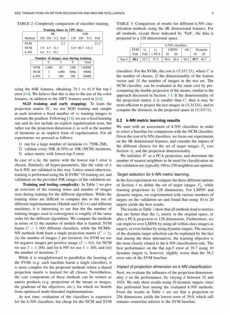
TABLE 2: Complexity comparison of classifier training.
Training times in CPU days4K 64K
Method 128 256 512 Full 128 256 512 Full
SVM 2.7 21.3NCM 1.9 4.5 12.1 32.9 80.3 141.2k-NN 4.6 5.1 10.1
Number of images seen during trainingC I T Total
SVM 1,000 65 120k 7,800MNCM 1 1,000 500k 500Mk-NN 1 300 2M 600M
using the 64K features, obtaining 78.1 vs 81.9 flat top-1error [44]. We believe that this is due to the use of the colorfeatures, in addition to the SIFT features used in [44].
SGD training and early stopping: To learn theprojection matrix W , we use SGD training and sampleat each iteration a fixed number of m training images toestimate the gradient. Following [24], we use a fixed learningrate and do not include an explicit regularization term, butrather use the projection dimension d, as well as the numberof iterations as an implicit form of regularization. For allexperiments we proceed as follows:
1) run for a large number of iterations (≈ 750K-2M),2) validate every 50K (k-NN) or 10K (NCM) iterations,3) select metric with lowest top-5 error.
In case of a tie, the metric with the lowest top-1 error ischosen. Similarly, all hyper-parameters, like the value of kfor k-NN, are validated in this way. Unless stated otherwise,training is performed using the ILSVRC’10 training set, andvalidation on the provided 50K images of the validation set.
Training and testing complexity: In Table 2 we givean overview of the training times and number of imagesseen during training for the different algorithms. While thetraining times are difficult to compare due to the use ofdifferent implementations (Matlab and C/C++) and differentmachines, it is interesting to see that the the number oftraining images used to convergence is roughly of the sameorder for the different algorithms. We compare the methodsin terms of (i) the number of models that is learned: SVMlearns C = 1, 000 different classifiers, while the NCM/k-NN methods both learn a single projection matrix (C = 1),(ii) the number of images I per iteration: for SVM we use64 negative images per positive image (I = 65), for NCMwe use I = 1, 000, and for k-NN we use I = 300, and (iii)the number of iterations T .
While it is straightforward to parallelize the learning ofthe SVMs (e.g . each machine learns a single classifier), itis more complex for the proposed methods where a sharedprojection matrix is learned for all classes. Nevertheless,the core components of these methods can be written asmatrix products (e.g . projections of the means or images,the gradients of the objectives, etc .), for which we benefitfrom optimized multi-threaded implementations.
At test time, evaluation of the classifiers is expensivefor the k-NN classifiers, but cheap for the NCM and SVM
TABLE 3: Comparison of results for different k-NN clas-sification methods using the 4K dimensional features. Forall methods, except those indicated by ‘Full’, the data isprojected to a 128 dimensional space.
k-NN classifiersSVM `2 `2 LMNN All DynamicFull Full + PCA 10 20 10 20
Top-5 38.2 55.7 57.3 50.6 50.4 44.2 39.7 40.7
classifiers. For the SVMs, the cost is O(MCD), where C isthe number of classes, D the dimensionality of the featurevector and M the number of images in the test set. TheNCM classifier, can be evaluated at the same cost by pre-computing the double projection of the means, similar to theapproach discussed in Section 3.4. If the dimensionality ofthe projection matrix d is smaller than C, then it may bemore efficient to project the test images in O(MDd), and tocompute the distances in the projected space in O(MCd).
5.2 k-NN metric learning resultsWe start with an assessment of k-NN classifiers in orderto select a baseline for comparison with the NCM classifier.Given the cost of k-NN classifiers, we focus our experimentson the 4K dimensional features, and consider the impact ofthe different choices for the set of target images Pq (seeSection 4), and the projection dimensionality.
We initialize W as a PCA projection, and determine thenumber of nearest neighbors to be used for classification onthe validation set; typically 100 to 250 neighbors are optimal.
Target selection for k-NN metric learning.In the first experiment we compare the three different optionsof Section 4 to define the set of target images Pq , whilelearning projections to 128 dimensions. For LMNN anddynamic targets, we experimented with various numbers oftargets on the validation set and found that using 10 to 20targets yields the best results.
The results in Table 3 show that all methods lead to metricsthat are better than the `2 metric in the original space, orafter a PCA projection to 128 dimensions. Furthermore, wecan improve over LMNN by using all within-class images astargets, or even further by using dynamic targets. The successof the dynamic target selection can be explained by the factthat among the three alternatives, the learning objective isthe most closely related to the k-NN classification rule. Thebest performance on the flat top-5 error of 39.7 using 10dynamic targets is, however, slightly worse than the 38.2error rate of the SVM baseline.
Impact of projection dimension on k-NN classification.Next, we evaluate the influence of the projection dimension-ality d on the performance, by varying d between 32 and1024. We only show results using 10 dynamic targets, sincethis performed best among the evaluated k-NN methods.From the results in Table 4 we see that a projection to256 dimensions yields the lowest error of 39.0, which stillremains somewhat inferior to the SVM baseline.
IEEE TRANSACTIONS ON PATTERN RECOGNITION AND MACHINE INTELLIGENCE 10
TABLE 4: Comparison on ILSVRC’10 of the k-NN andNCM classifiers with related methods, using the 4K and 64Kdimensional features and for various projection dimensions.
4K dimensional featuresProjection dim. 32 64 128 256 512 1024 Full
SVM baseline 38.2k-NN, dynamic 10 47.2 42.2 39.7 39.0 39.4 42.4NCM, NCMML 49.1 42.7 39.0 37.4 37.0 37.0NCM, FDA 65.2 59.4 54.6 52.0 50.8 50.5NCM, PCA + `2 78.7 74.6 71.7 69.9 68.8 68.2 68.0NCM, PCA + inv. cov. 75.5 67.7 60.6 54.5 49.3 46.1 43.8Ridge-regression, PCA 86.3 80.3 73.9 68.1 62.8 58.9 54.6WSABIE 51.9 45.1 41.2 39.4 38.7 38.5
64K dimensional featuresSVM baseline 28.0NCMML and `2 31.7 31.0 30.7 63.2WSABIE 32.2 30.1 29.2
5.3 Nearest class mean classifier results
We now consider the performance of NCM classifiers andthe related methods described in Section 3. For all experi-ments we use the NCM with Euclidean distance accordingto Eq. (5). In Table 4 we show the results.
We first consider the results for the 4K dimensionalfeatures. As observed for the k-NN classifier, also for NCMusing a learned metric outperforms using the `2 distance(68.0); which is worse than using `2 distances for the k-NN classifier (55.7, see Table 3). However, unexpectedly,with metric learning we observe that our NCM classifier(37.0) outperforms the more flexible k-NN classifier (39.0),as well as the SVM baseline (38.2) when projecting to 256dimensions or more. Our implementation of WSABIE [3]scores slightly worse (38.5) than the baseline and our NCMclassifier, and does not generalize to new classes withoutretraining.
We also compare our NCM classifier to several otheralgorithms which do allow generalization to new classes.First, we consider two other supervised metric learningapproaches, NCM with FDA (which leads to 50.5) andridge-regression (which leads to 54.6). We observe thatNCMML outperforms both methods significantly. Second,we consider two unsupervised variants of the NCM classifierwhere we use PCA to reduce the dimensionality. In one casewe use the `2 metric after PCA. In the other, inspired byridge-regression, we use NCM with the metric W generatedby the inverse of the regularized covariance matrix, suchthat W>W = (Σ + λI)−1, see Section 3.2. We tunedthe regularization parameter λ on the validation set, as wasalso done for ridge-regression. From these results we canconclude that, just like for k-NN, the `2 metric with orwithout PCA leads to poor results (68.0) as compared toa learned metric. Also, the feature whitening implementedby the inverse covariance metric leads to results (43.8) thatare better than using the `2 metric, and also substantiallybetter than ridge-regression (54.6). The results are howeversignificantly worse than using our learned metric, in partic-ular when using low-rank metrics.
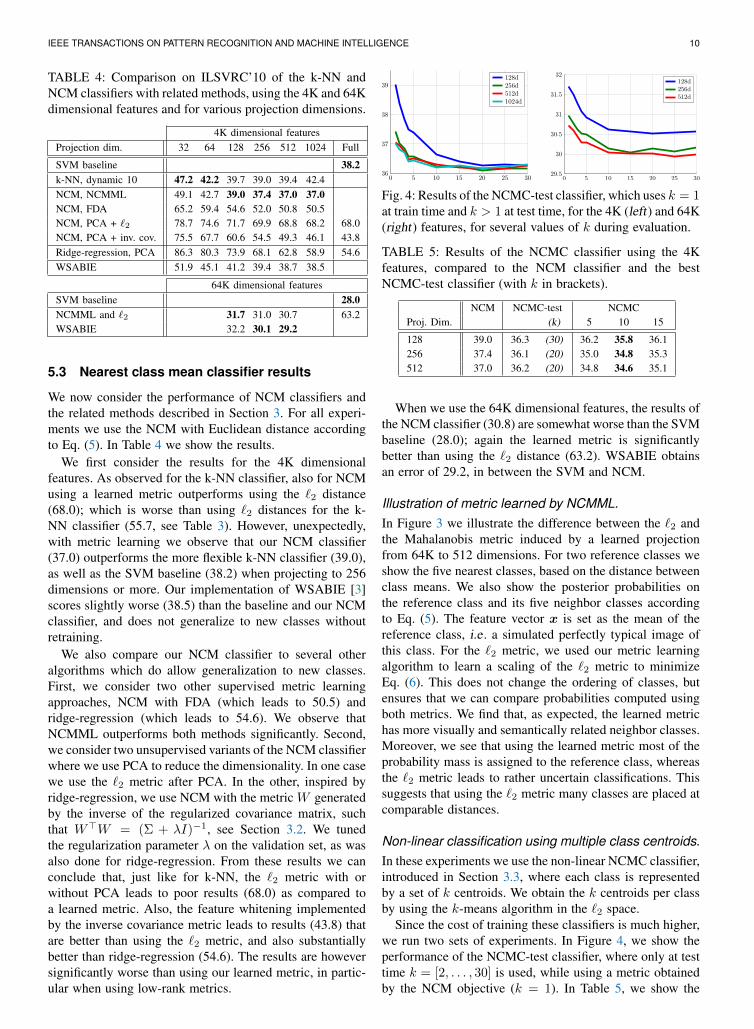
0 5 10 15 20 25 3036
37
38
39128d256d512d1024d
0 5 10 15 20 25 3029.5
30
30.5
31
31.5
32128d256d512d
Fig. 4: Results of the NCMC-test classifier, which uses k = 1at train time and k > 1 at test time, for the 4K (left) and 64K(right) features, for several values of k during evaluation.
TABLE 5: Results of the NCMC classifier using the 4Kfeatures, compared to the NCM classifier and the bestNCMC-test classifier (with k in brackets).
NCM NCMC-test NCMCProj. Dim. (k) 5 10 15
128 39.0 36.3 (30) 36.2 35.8 36.1256 37.4 36.1 (20) 35.0 34.8 35.3512 37.0 36.2 (20) 34.8 34.6 35.1
When we use the 64K dimensional features, the results ofthe NCM classifier (30.8) are somewhat worse than the SVMbaseline (28.0); again the learned metric is significantlybetter than using the `2 distance (63.2). WSABIE obtainsan error of 29.2, in between the SVM and NCM.
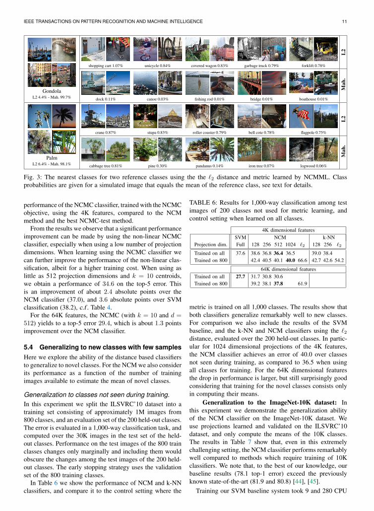
Illustration of metric learned by NCMML.In Figure 3 we illustrate the difference between the `2 andthe Mahalanobis metric induced by a learned projectionfrom 64K to 512 dimensions. For two reference classes weshow the five nearest classes, based on the distance betweenclass means. We also show the posterior probabilities onthe reference class and its five neighbor classes accordingto Eq. (5). The feature vector x is set as the mean of thereference class, i.e . a simulated perfectly typical image ofthis class. For the `2 metric, we used our metric learningalgorithm to learn a scaling of the `2 metric to minimizeEq. (6). This does not change the ordering of classes, butensures that we can compare probabilities computed usingboth metrics. We find that, as expected, the learned metrichas more visually and semantically related neighbor classes.Moreover, we see that using the learned metric most of theprobability mass is assigned to the reference class, whereasthe `2 metric leads to rather uncertain classifications. Thissuggests that using the `2 metric many classes are placed atcomparable distances.
Non-linear classification using multiple class centroids.In these experiments we use the non-linear NCMC classifier,introduced in Section 3.3, where each class is representedby a set of k centroids. We obtain the k centroids per classby using the k-means algorithm in the `2 space.
Since the cost of training these classifiers is much higher,we run two sets of experiments. In Figure 4, we show theperformance of the NCMC-test classifier, where only at testtime k = [2, . . . , 30] is used, while using a metric obtainedby the NCM objective (k = 1). In Table 5, we show the
IEEE TRANSACTIONS ON PATTERN RECOGNITION AND MACHINE INTELLIGENCE 11
GondolaL2 4.4% - Mah. 99.7%
shopping cart 1.07% unicycle 0.84% covered wagon 0.83% garbage truck 0.79% forklift 0.78%
L2
dock 0.11% canoe 0.03% fishing rod 0.01% bridge 0.01% boathouse 0.01%
Mah
.
PalmL2 6.4% - Mah. 98.1%
crane 0.87% stupa 0.83% roller coaster 0.79% bell cote 0.78% flagpole 0.75%
L2
cabbage tree 0.81% pine 0.30% pandanus 0.14% iron tree 0.07% logwood 0.06%
Mah
.
Fig. 3: The nearest classes for two reference classes using the the `2 distance and metric learned by NCMML. Classprobabilities are given for a simulated image that equals the mean of the reference class, see text for details.
performance of the NCMC classifier, trained with the NCMCobjective, using the 4K features, compared to the NCMmethod and the best NCMC-test method.
From the results we observe that a significant performanceimprovement can be made by using the non-linear NCMCclassifier, especially when using a low number of projectiondimensions. When learning using the NCMC classifier wecan further improve the performance of the non-linear clas-sification, albeit for a higher training cost. When using aslittle as 512 projection dimensions and k = 10 centroids,we obtain a performance of 34.6 on the top-5 error. Thisis an improvement of about 2.4 absolute points over theNCM classifier (37.0), and 3.6 absolute points over SVMclassification (38.2), c.f . Table 4.
For the 64K features, the NCMC (with k = 10 and d =512) yields to a top-5 error 29.4, which is about 1.3 pointsimprovement over the NCM classifier.
5.4 Generalizing to new classes with few samplesHere we explore the ability of the distance based classifiersto generalize to novel classes. For the NCM we also considerits performance as a function of the number of trainingimages available to estimate the mean of novel classes.
Generalization to classes not seen during training.In this experiment we split the ILSVRC’10 dataset into atraining set consisting of approximately 1M images from800 classes, and an evaluation set of the 200 held-out classes.The error is evaluated in a 1,000-way classification task, andcomputed over the 30K images in the test set of the held-out classes. Performance on the test images of the 800 trainclasses changes only marginally and including them wouldobscure the changes among the test images of the 200 held-out classes. The early stopping strategy uses the validationset of the 800 training classes.
In Table 6 we show the performance of NCM and k-NNclassifiers, and compare it to the control setting where the
TABLE 6: Results for 1,000-way classification among testimages of 200 classes not used for metric learning, andcontrol setting when learned on all classes.
4K dimensional featuresSVM NCM k-NN
Projection dim. Full 128 256 512 1024 `2 128 256 `2
Trained on all 37.6 38.6 36.8 36.4 36.5 39.0 38.4Trained on 800 42.4 40.5 40.1 40.0 66.6 42.7 42.6 54.2
64K dimensional featuresTrained on all 27.7 31.7 30.8 30.6Trained on 800 39.2 38.1 37.8 61.9
metric is trained on all 1,000 classes. The results show thatboth classifiers generalize remarkably well to new classes.For comparison we also include the results of the SVMbaseline, and the k-NN and NCM classifiers using the `2distance, evaluated over the 200 held-out classes. In partic-ular for 1024 dimensional projections of the 4K features,the NCM classifier achieves an error of 40.0 over classesnot seen during training, as compared to 36.5 when usingall classes for training. For the 64K dimensional featuresthe drop in performance is larger, but still surprisingly goodconsidering that training for the novel classes consists onlyin computing their means.
Generalization to the ImageNet-10K dataset: Inthis experiment we demonstrate the generalization abilityof the NCM classifier on the ImageNet-10K dataset. Weuse projections learned and validated on the ILSVRC’10dataset, and only compute the means of the 10K classes.The results in Table 7 show that, even in this extremelychallenging setting, the NCM classifier performs remarkablywell compared to methods which require training of 10Kclassifiers. We note that, to the best of our knowledge, ourbaseline results (78.1 top-1 error) exceed the previouslyknown state-of-the-art (81.9 and 80.8) [44], [45].
Training our SVM baseline system took 9 and 280 CPU

IEEE TRANSACTIONS ON PATTERN RECOGNITION AND MACHINE INTELLIGENCE 12
TABLE 7: Comparison of the results on the ImageNet-10K dataset: the NCM classifier with metrics learned on theILSVRC’10 dataset, the NCM using `2 distance, the baseline SVM, and previously reported SVM results [1], [7], [44] andthe Deep Learning results of [45].
4K dimensional features 64K dimensional features Previous ResultsMethod NCM SVM NCM SVM [7] [1] [44] [45]Proj. dim. 128 256 512 1024 `2 4K 128 256 512 `2 64K 21K 131K 128K
Top-1 error 91.8 90.6 90.5 90.4 95.5 86.0 87.1 86.3 86.1 93.6 78.1 93.6 83.3 81.9 80.8Top-5 error 80.7 78.7 78.6 78.6 89.0 72.4 71.7 70.5 70.1 85.4 60.9
days respectively for the 4K and 64K features, while thecomputation of the means for the NCM classifier tookapproximately 3 and 48 CPU minutes respectively. Thisrepresents roughly a 8,500 fold speed-up as compared tothe SVMs, given a learned projection matrix.
Accuracy as function of sample size of novel classes.In this experiment we consider the error as a function of thenumber of images that are used to compute the means ofnovel classes. Inspired by [38], we also include a zero-shotlearning experiment, where we use the ImageNet hierarchyto estimate the mean of novel classes from related classes.We estimate the mean of a novel class µz using the meansof its ancestor nodes in the ILSVRC’10 class hierarchy:
µz =1
|Az|∑a∈Az
µa, (29)
where Az denotes the set of ancestors of node z, and µa isthe mean of ancestor a. The mean of an internal node, µa, iscomputed as the average of the means of all its descendanttraining classes.
If we view the estimation of each class mean as theestimation of the mean of a Gaussian distribution, then themean of a sample of imagesµs corresponds to the MaximumLikelihood (ML) estimate, while the zero-shot estimate µz
can be thought of as a prior. To obtain a maximum a-posteriori (MAP) estimate µp, we combine the prior andthe ML estimate as follows:
µp =nµs +mµz
n+m, (30)
where the ML estimate is weighed by n the number ofimages that were used to compute it, and the prior meanobtains a weight m determined on the validation set [46].
In Figure 5 we analyze the performance of the NCMclassifier trained on the images of the same 800 classesused above, with a learned projection from 4K and 64Kto 512 dimensions. The metric and the parameter m arevalidated using the images of the 200 held-out classes of thevalidation set. We again report the error on the test images ofthe held-out classes in a 1,000-way classification as above.We repeat the experiment 10 times, and show error-bars atthree times standard deviation. For the error to stabilize weonly need approximately 100 images to estimate the classmeans. The results show that the zero-shot prior can beeffectively combined with the empirical mean to providea smooth transition from the zero-shot setting to a settingwith many training examples. Inclusion of the zero-shot prior
0 1 10 100 100020
40
60
80
100
0 1 10 100 100020
40
60
80
100ML MAP Baseline
Fig. 5: Results of NCM as a function of the number of imagesused to compute the means for test classes. Comparison ofthe ML (blue) and MAP (red ) mean estimates, for the 4K(left) and 64K (right) features, in a 1,000-way classificationtask, including baseline (black ) when trained on all classes.
leads to a significant error reduction in the regime where tenimages or less are available. Also, the results show that thevalidation on the 200 hold-out classes or on the 800 trainingclasses yields comparable error rates (40.1 vs 39.9, using4K and 512d, c.f . Table 6 and Figure 5).
In [38] a zero-shot error rate of 65.2 was reported in a200-way classification task. Using the NCM with our priormean estimates leads to comparable error rates of 66.5 (4K)and 64.0 (64K). Note that a different set of 200 hold-outclasses were used, as well as different features. Howevertheir baseline performance of 37.6 top-5 error is comparableto our 4K features (38.2).
Instance level image retrieval.Query-by-example image retrieval can be seen as an imageclassification problem where only a single positive sample(the query) is given and negative examples are not explicitlyprovided. Recently, using classifiers to learn a metric forimage retrieval was considered in [47]. They found theJoint Subspace and Classifier Learning (JSCL) method tobe the most effective. It consists of learning jointly a setof classifiers and a projection matrix W using WSABIE,Eq. (12) on an auxiliary supervised dataset. After training,the learned projection matrixW is used to compute distancesbetween queries and database images.
Similarly, we propose to learn a metric using our NCMclassifier on the auxiliary supervised dataset and to use thelearned metric to retrieve the most similar images for a givenquery.
For this experiment we use the same public benchmarksas in [47]. First, the INRIA Holidays data set [48], whichconsists of 1,491 images of 500 scenes and objects. For
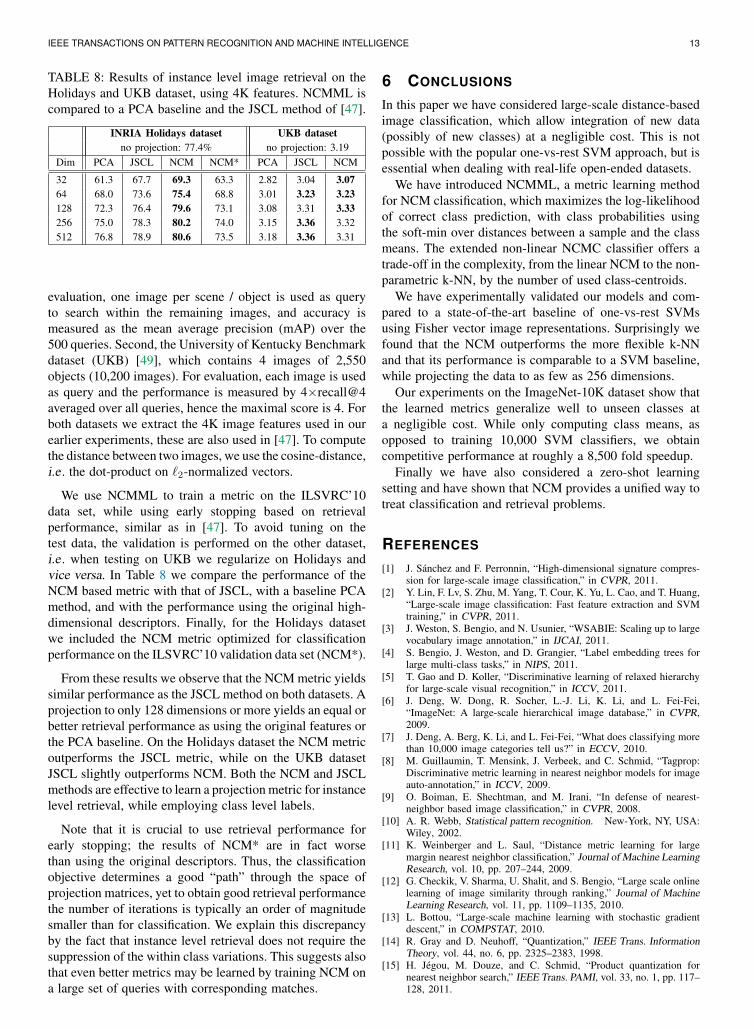
IEEE TRANSACTIONS ON PATTERN RECOGNITION AND MACHINE INTELLIGENCE 13
TABLE 8: Results of instance level image retrieval on theHolidays and UKB dataset, using 4K features. NCMML iscompared to a PCA baseline and the JSCL method of [47].
INRIA Holidays dataset UKB datasetno projection: 77.4% no projection: 3.19
Dim PCA JSCL NCM NCM* PCA JSCL NCM
32 61.3 67.7 69.3 63.3 2.82 3.04 3.0764 68.0 73.6 75.4 68.8 3.01 3.23 3.23128 72.3 76.4 79.6 73.1 3.08 3.31 3.33256 75.0 78.3 80.2 74.0 3.15 3.36 3.32512 76.8 78.9 80.6 73.5 3.18 3.36 3.31
evaluation, one image per scene / object is used as queryto search within the remaining images, and accuracy ismeasured as the mean average precision (mAP) over the500 queries. Second, the University of Kentucky Benchmarkdataset (UKB) [49], which contains 4 images of 2,550objects (10,200 images). For evaluation, each image is usedas query and the performance is measured by 4×recall@4averaged over all queries, hence the maximal score is 4. Forboth datasets we extract the 4K image features used in ourearlier experiments, these are also used in [47]. To computethe distance between two images, we use the cosine-distance,i.e . the dot-product on `2-normalized vectors.
We use NCMML to train a metric on the ILSVRC’10data set, while using early stopping based on retrievalperformance, similar as in [47]. To avoid tuning on thetest data, the validation is performed on the other dataset,i.e . when testing on UKB we regularize on Holidays andvice versa. In Table 8 we compare the performance of theNCM based metric with that of JSCL, with a baseline PCAmethod, and with the performance using the original high-dimensional descriptors. Finally, for the Holidays datasetwe included the NCM metric optimized for classificationperformance on the ILSVRC’10 validation data set (NCM*).
From these results we observe that the NCM metric yieldssimilar performance as the JSCL method on both datasets. Aprojection to only 128 dimensions or more yields an equal orbetter retrieval performance as using the original features orthe PCA baseline. On the Holidays dataset the NCM metricoutperforms the JSCL metric, while on the UKB datasetJSCL slightly outperforms NCM. Both the NCM and JSCLmethods are effective to learn a projection metric for instancelevel retrieval, while employing class level labels.
Note that it is crucial to use retrieval performance forearly stopping; the results of NCM* are in fact worsethan using the original descriptors. Thus, the classificationobjective determines a good “path” through the space ofprojection matrices, yet to obtain good retrieval performancethe number of iterations is typically an order of magnitudesmaller than for classification. We explain this discrepancyby the fact that instance level retrieval does not require thesuppression of the within class variations. This suggests alsothat even better metrics may be learned by training NCM ona large set of queries with corresponding matches.
6 CONCLUSIONS
In this paper we have considered large-scale distance-basedimage classification, which allow integration of new data(possibly of new classes) at a negligible cost. This is notpossible with the popular one-vs-rest SVM approach, but isessential when dealing with real-life open-ended datasets.
We have introduced NCMML, a metric learning methodfor NCM classification, which maximizes the log-likelihoodof correct class prediction, with class probabilities usingthe soft-min over distances between a sample and the classmeans. The extended non-linear NCMC classifier offers atrade-off in the complexity, from the linear NCM to the non-parametric k-NN, by the number of used class-centroids.
We have experimentally validated our models and com-pared to a state-of-the-art baseline of one-vs-rest SVMsusing Fisher vector image representations. Surprisingly wefound that the NCM outperforms the more flexible k-NNand that its performance is comparable to a SVM baseline,while projecting the data to as few as 256 dimensions.
Our experiments on the ImageNet-10K dataset show thatthe learned metrics generalize well to unseen classes ata negligible cost. While only computing class means, asopposed to training 10,000 SVM classifiers, we obtaincompetitive performance at roughly a 8,500 fold speedup.
Finally we have also considered a zero-shot learningsetting and have shown that NCM provides a unified way totreat classification and retrieval problems.
REFERENCES
[1] J. Sanchez and F. Perronnin, “High-dimensional signature compres-sion for large-scale image classification,” in CVPR, 2011.
[2] Y. Lin, F. Lv, S. Zhu, M. Yang, T. Cour, K. Yu, L. Cao, and T. Huang,“Large-scale image classification: Fast feature extraction and SVMtraining,” in CVPR, 2011.
[3] J. Weston, S. Bengio, and N. Usunier, “WSABIE: Scaling up to largevocabulary image annotation,” in IJCAI, 2011.
[4] S. Bengio, J. Weston, and D. Grangier, “Label embedding trees forlarge multi-class tasks,” in NIPS, 2011.
[5] T. Gao and D. Koller, “Discriminative learning of relaxed hierarchyfor large-scale visual recognition,” in ICCV, 2011.
[6] J. Deng, W. Dong, R. Socher, L.-J. Li, K. Li, and L. Fei-Fei,“ImageNet: A large-scale hierarchical image database,” in CVPR,2009.
[7] J. Deng, A. Berg, K. Li, and L. Fei-Fei, “What does classifying morethan 10,000 image categories tell us?” in ECCV, 2010.
[8] M. Guillaumin, T. Mensink, J. Verbeek, and C. Schmid, “Tagprop:Discriminative metric learning in nearest neighbor models for imageauto-annotation,” in ICCV, 2009.
[9] O. Boiman, E. Shechtman, and M. Irani, “In defense of nearest-neighbor based image classification,” in CVPR, 2008.
[10] A. R. Webb, Statistical pattern recognition. New-York, NY, USA:Wiley, 2002.
[11] K. Weinberger and L. Saul, “Distance metric learning for largemargin nearest neighbor classification,” Journal of Machine LearningResearch, vol. 10, pp. 207–244, 2009.
[12] G. Checkik, V. Sharma, U. Shalit, and S. Bengio, “Large scale onlinelearning of image similarity through ranking,” Journal of MachineLearning Research, vol. 11, pp. 1109–1135, 2010.
[13] L. Bottou, “Large-scale machine learning with stochastic gradientdescent,” in COMPSTAT, 2010.
[14] R. Gray and D. Neuhoff, “Quantization,” IEEE Trans. InformationTheory, vol. 44, no. 6, pp. 2325–2383, 1998.
[15] H. Jegou, M. Douze, and C. Schmid, “Product quantization fornearest neighbor search,” IEEE Trans. PAMI, vol. 33, no. 1, pp. 117–128, 2011.

IEEE TRANSACTIONS ON PATTERN RECOGNITION AND MACHINE INTELLIGENCE 14
[16] F. Perronnin, J. Sanchez, and T. Mensink, “Improving the Fisherkernel for large-scale image classification,” in ECCV, 2010.
[17] T. Mensink, J. Verbeek, F. Perronnin, and G. Csurka, “Metriclearning for large scale image classification: Generalizing to newclasses at near-zero cost,” in ECCV, 2012.
[18] G. Csurka, C. Dance, L. Fan, J. Willamowski, and C. Bray, “Visualcategorization with bags of keypoints,” in ECCV Int. Workshop onStat. Learning in Computer Vision, 2004.
[19] J. Zhang, M. Marszałek, S. Lazebnik, and C. Schmid, “Local featuresand kernels for classification of texture and object categories: acomprehensive study,” IJCV, vol. 73, no. 2, pp. 213–238, 2007.
[20] H. Jegou, F. Perronnin, M. Douze, J. Sanchez, P. Perez, andC. Schmid, “Aggregating local image descriptors into compactcodes,” IEEE Trans. PAMI, 2012, to appear.
[21] E. Nowak and F. Jurie, “Learning visual similarity measures forcomparing never seen objects,” in CVPR, 2007.
[22] M. Guillaumin, J. Verbeek, and C. Schmid, “Is that you? Metriclearning approaches for face identification,” in ICCV, 2009.
[23] M. Kostinger, M. Hirzer, P. Wohlhart, P. M. Roth, and H. Bischof,“Large scale metric learning from equivalence constraints,” in CVPR,2012.
[24] B. Bai, J. Weston, D. Grangier, R. Collobert, Y. Qi, K. Sadamasa,O. Chapelle, and K. Weinberger, “Learning to rank with (a lot of)word features,” Information Retrieval – Special Issue on Learning toRank, vol. 13, pp. 291–314, 2010.
[25] J. Chai, H. Liua, B. Chenb, and Z. Baoa, “Large margin nearestlocal mean classifier,” Signal Processing, vol. 90, no. 1, pp. 236–248, 2010.
[26] A. Globerson and S. Roweis, “Metric learning by collapsing classes,”in NIPS, 2006.
[27] J. Goldberger, S. Roweis, G. Hinton, and R. Salakhutdinov, “Neigh-bourhood component analysis,” in NIPS, 2005.
[28] C. Veenman and D. Tax, “LESS: a model-based classifier for sparsesubspaces,” IEEE Trans. PAMI, vol. 27, no. 9, pp. 1496–1500, 2005.
[29] K. Weinberger and O. Chapelle, “Large margin taxonomy embeddingfor document categorization,” in NIPS, 2009.
[30] X. Zhou, X. Zhang, Z. Yan, S.-F. Chang, M. Hasegawa-Johnson,and T. Huang, “Sift-bag kernel for video event analysis,” in ACMMultimedia, 2008.
[31] Z. Wang, Y. Hu, and L.-T. Chia, “Image-to-class distance metriclearning for image classification,” in ECCV, 2010.
[32] L. Fei-Fei, R. Fergus, and P. Perona, “One-shot learning of objectcategories,” IEEE Trans. PAMI, vol. 28, no. 4, pp. 594–611, 2006.
[33] C. Lampert, H. Nickisch, and S. Harmeling, “Learning to detectunseen object classes by between-class attribute transfer,” in CVPR,2009.
[34] T. Tommasi and B. Caputo, “The more you know, the less you learn:from knowledge transfer to one-shot learning of object categories,”in BMVC, 2009.
[35] H. Larochelle, D. Erhan, and Y. Bengio, “Zero-data learning of newtasks,” in AAAI Conference on Artificial Intelligence, 2008.
[36] K. Saenko, B. Kulis, M. Fritz, and T. Darrell, “Adapting visualcategory models to new domains,” in ECCV, 2010.
[37] S. Parameswaran and K. Weinberger, “Large margin multi-taskmetric learning,” in NIPS, 2010.
[38] M. Rohrbach, M. Stark, and B. Schiele, “Evaluating knowledgetransfer and zero-shot learning in a large-scale setting,” in CVPR,2011.
[39] A. Lucchi and J. Weston., “Joint image and word sense discrimina-tion for image retrieval,” in ECCV, 2012.
[40] S. Boyd and L. Vandenberghe, Convex Optimization. CambridgeUniversity Press, 2004.
[41] T. Mensink, J. Verbeek, F. Perronnin, and G. Csurka, “Largescale metric learning for distance-based image classification,”INRIA, Research Report RR-8077, 2012. [Online]. Available:http://hal.inria.fr/hal-00735908
[42] D. Lowe, “Distinctive image features from scale-invariant key-points,” IJCV, vol. 60, no. 2, pp. 91–110, 2004.
[43] S. Clinchant, G. Csurka, F. Perronnin, and J.-M. Renders, “XRCE’sparticipation to ImagEval,” in ImageEval Workshop at CVIR, 2007.
[44] F. Perronnin, Z. Akata, Z. Harchaoui, and C. Schmid, “Towards goodpractice in large-scale learning for image classification,” in CVPR,2012.
[45] Q. Le, M. Ranzato, R. Monga, M. Devin, K.Chen, G. Corrado,J. Dean, and A. Ng, “Building high-level features using large scaleunsupervised learning,” in ICML, 2012.
[46] J.-L. Gauvain and C.-H. Lee, “Maximum a posteriori estimation formultivariate Gaussian mixture observations of Markov chains.” IEEETrans. Speech and Audio Processing, vol. 2, no. 2, pp. 291–298,1994.
[47] A. Gordo, J. Rodrıguez, F. Perronnin, and E. Valveny, “Leveragingcategory-level labels for instance-level image retrieval,” in CVPR,2012.
[48] H. Jegou, M. Douze, and C. Schmid, “Hamming embedding andweak geometric consistency for large scale image search,” in ECCV,2008.
[49] D. Nister and H. Stewenius, “Scalable recognition with a vocabularytree,” in CVPR, 2006.
Thomas Mensink received a PhD degree incomputer science in 2012 from the Universityof Grenoble, France, and a cum laude MScdegree in artificial intelligence from the Uni-versity of Amsterdam, The Netherlands. Dur-ing the research for his PhD he worked bothat Xerox Research Centre Europe and at theLEAR team of INRIA Grenoble. Currently heis PostDoc at the University of Amsterdam.His research interests include machine learn-ing and computer vision.
Jakob Verbeek received a PhD degree incomputer science in 2004 from the Universityof Amsterdam, The Netherlands. After beinga postdoctoral researcher at the Universityof Amsterdam and at INRIA Rhone-Alpes,he has been a full-time researcher at INRIA,Grenoble, France, since 2007. His researchinterests include machine learning and com-puter vision, with special interest in applica-tions of statistical models in computer vision.
Florent Perronnin holds an Engineering de-gree from the Ecole Nationale Superieuredes Telecommunications and a PhD degreefrom the Ecole Polytechnique Federale deLausanne. From 2000 to 2001 he was aResearcher in the Panasonic Speech Tech-nology Laboratory working on speech andspeaker recognition. In 2005, he joined theXerox Research Centre Europe where he iscurrently a Principal Scientist and the Man-ager of the Computer Vision Group. His main
interests are in the application of machine learning to problems suchas image classification, retrieval and segmentation.
Gabriela Csurka obtained her Ph.D. degreein computer science in 1996 from Univer-sity of Nice Sophia Antipolis. She worked infields such as stereo vision and projectivereconstruction at INRIA and image water-marking at University of Geneva and Insti-tute Eurecom. In 2002 she joined the XeroxResearch Centre Europe, where she is se-nior scientist. Her research interest includemono-modal and multi-modal image catego-rization, retrieval and semantic image seg-
mentation.