dissipative wave equations: theory, numerics & optimal design · dissipative wave equations:...
TRANSCRIPT
Outline
Dissipative wave equations: theory, numerics &optimal design
Enrique Zuazua
Departamento de MatematicasUniversidad Autonoma de Madrid
Paris-Sud, Orsay, Numerical Analysis Seminar, December 2006
Enrique Zuazua Dissipative wave equations: theory, numerics & optimal design

Outline
Outline
Enrique Zuazua Dissipative wave equations: theory, numerics & optimal design

Outline
Outline
1 Introduction
2 Geometric issues on the stabilization of waves
3 Characterizing the exponential decay rate
4 Optimal design of dampers
5 Numerical approximation
6 Numerical viscosity
Enrique Zuazua Dissipative wave equations: theory, numerics & optimal design

Outline
Outline
1 Introduction
2 Geometric issues on the stabilization of waves
3 Characterizing the exponential decay rate
4 Optimal design of dampers
5 Numerical approximation
6 Numerical viscosity
Enrique Zuazua Dissipative wave equations: theory, numerics & optimal design

Outline
Outline
1 Introduction
2 Geometric issues on the stabilization of waves
3 Characterizing the exponential decay rate
4 Optimal design of dampers
5 Numerical approximation
6 Numerical viscosity
Enrique Zuazua Dissipative wave equations: theory, numerics & optimal design

Outline
Outline
1 Introduction
2 Geometric issues on the stabilization of waves
3 Characterizing the exponential decay rate
4 Optimal design of dampers
5 Numerical approximation
6 Numerical viscosity
Enrique Zuazua Dissipative wave equations: theory, numerics & optimal design
Outline
Outline
1 Introduction
2 Geometric issues on the stabilization of waves
3 Characterizing the exponential decay rate
4 Optimal design of dampers
5 Numerical approximation
6 Numerical viscosity
Enrique Zuazua Dissipative wave equations: theory, numerics & optimal design

Outline
Outline
1 Introduction
2 Geometric issues on the stabilization of waves
3 Characterizing the exponential decay rate
4 Optimal design of dampers
5 Numerical approximation
6 Numerical viscosity
Enrique Zuazua Dissipative wave equations: theory, numerics & optimal design

Intro Geometry Characterization Optimization Numerics Viscoity
Motivation
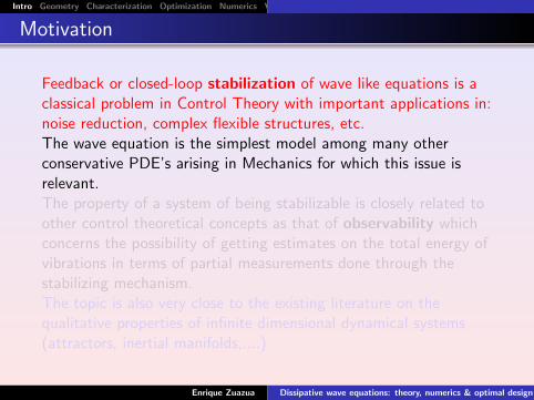
Feedback or closed-loop stabilization of wave like equations is aclassical problem in Control Theory with important applications in:noise reduction, complex flexible structures, etc.The wave equation is the simplest model among many otherconservative PDE’s arising in Mechanics for which this issue isrelevant.The property of a system of being stabilizable is closely related toother control theoretical concepts as that of observability whichconcerns the possibility of getting estimates on the total energy ofvibrations in terms of partial measurements done through thestabilizing mechanism.The topic is also very close to the existing literature on thequalitative properties of infinite dimensional dynamical systems(attractors, inertial manifolds,....)
Enrique Zuazua Dissipative wave equations: theory, numerics & optimal design
Intro Geometry Characterization Optimization Numerics Viscoity
Motivation
Feedback or closed-loop stabilization of wave like equations is aclassical problem in Control Theory with important applications in:noise reduction, complex flexible structures, etc.The wave equation is the simplest model among many otherconservative PDE’s arising in Mechanics for which this issue isrelevant.The property of a system of being stabilizable is closely related toother control theoretical concepts as that of observability whichconcerns the possibility of getting estimates on the total energy ofvibrations in terms of partial measurements done through thestabilizing mechanism.The topic is also very close to the existing literature on thequalitative properties of infinite dimensional dynamical systems(attractors, inertial manifolds,....)
Enrique Zuazua Dissipative wave equations: theory, numerics & optimal design

Intro Geometry Characterization Optimization Numerics Viscoity
An example: Boundary stabilization of the wave equationLet Ω be a bounded domain of Rn, n ≥ 1, with boundary Γ of classC 2 and Γ0 be an open and non-empty subset of Γ.
ytt −∆y = 0 in Q = Ω× (0,∞)y = 0 on Σ1 = (Γ \ Γ0)× (0,∞)∂y∂ν = −yt on Σ0 = Γ0 × (0,∞)y(x , 0) = y0(x), yt(x , 0) = y1(x) in Ω.
The energy is then of the form
E (t) =1
2
∫Ω
[|yt |2 + |∇y |2
]dx
and satisfies the energy dissipation law
dE (t)
dt= −
∫Γ0
|yt |2dΓ.
Enrique Zuazua Dissipative wave equations: theory, numerics & optimal design

Intro Geometry Characterization Optimization Numerics Viscoity
A variant: Internal stabilization. Let ω be an open subset of Ω.Consider:
ytt −∆y =−yt1ω in Q = Ω× (0,∞)y = 0 on Σ = Γ× (0,∞)y(x , 0) = y0(x), yt(x , 0) = y1(x) in Ω,
where 1ω stands for the characteristic function of the subset ω.The energy dissipation law is then
dE (t)
dt= −
∫ω|yt |2dx .
Question: Do they exist C > 0 and γ > 0 such that
E (t) ≤ Ce−γtE (0), ∀t ≥ 0,
for all solution of the dissipative system?
Enrique Zuazua Dissipative wave equations: theory, numerics & optimal design

Intro Geometry Characterization Optimization Numerics Viscoity
This is equivalent to an observability property: There exists C > 0and T > 0 such that
E (0) ≤ C
∫ T
0
∫ω|yt |2dxdt.
In other words, the exponential decay property is equivalent toshowing that the dissipated energy within an interval [0,T ]contains a fraction of the initial energy, uniformly for all solutions.This estimate, together with the energy dissipation law, shows that
E (T ) ≤ σE (0)
with 0 < σ < 1. Accordingly the semigroup map S(T ) is a strictcontraction. By the semigroup property one deduces immediatelythe exponential decay rate.Note that, for dissipative semigroups, the following alternativeholds: Either ||S(t)|| = 1 for all t ≥ 0 or ||S(T )|| < 1 for someT > 0 and then the energy decays exponentially as t →∞.
Enrique Zuazua Dissipative wave equations: theory, numerics & optimal design

Intro Geometry Characterization Optimization Numerics Viscoity
The observability inequality and, accordingly, the exponential decayproperty holds if and only if the support of the dissipativemechanism, Γ0 or ω, satisfies the so called the Geometric ControlCondition (GCC) (Ralston, Rauch-Taylor,Bardos-Lebeau-Rauch,...)
Rays propagating inside the domain Ω following straight lines thatare reflected on the boundary according to the laws of GeometricOptics. The control region is the red subset of the boundary. TheGCC is satisfied in this case. The proof requires tools fromMicrolocal Analysis.
Enrique Zuazua Dissipative wave equations: theory, numerics & optimal design

Intro Geometry Characterization Optimization Numerics Viscoity
The Geometric Control Condition is not satisfied, whatever T > 0is, in the square domain when the control is located on a subset oftwo consecutive sides of the boundary, leaving a subsegmentuncontrolled. There is an horizontal a ray that bounces back andforth for all time perpendicularly on two points of the verticalboundaries where the control does not act.
Enrique Zuazua Dissipative wave equations: theory, numerics & optimal design

Intro Geometry Characterization Optimization Numerics Viscoity
When the GCC fails, the uniform exponential decay property doesnot hold. In that case one only gets a logarithmic decay rate forsolutions with initial data in H2 × H1. 1 This result is sharp ingeneral and it is in agreement with the exponential rate ofconcentration of gaussian beams along non-observed rays.
1L. Robbiano, Fonction de cout et controle des solutions des equationshyperboliques, Asymptotic Anal., 10 (1995), 95–115.
Enrique Zuazua Dissipative wave equations: theory, numerics & optimal design

Intro Geometry Characterization Optimization Numerics Viscoity
Often, in particular, in the context of internal stabilization andessentally also in the boundary stabilization problem, it suffices toprove the observability property for the undamped system:
ϕtt −∆ϕ = 0 in Q = Ω× (0,T )ϕ = 0 on Σ = Γ× (0,T )ϕ(x , 0) = ϕ0(x), ϕt(x , 0) = ϕ1(x) in Ω.
The problem is then reduced to showing that:
E0 ≤ C (Γ0,T )
∫Γ0×(0,T )
∣∣∣∂ϕ
∂ν
∣∣∣2dσdt ?
A sharp discussion of this inequality requires of Microlocal analysis.Partial results may be obtained by means of multipliers: x · ∇ϕ,ϕt , ϕ,...Similar problems arise in Control, Optimal Design and in InverseProblems Theory and common techniques need to be developed.
Enrique Zuazua Dissipative wave equations: theory, numerics & optimal design

Intro Geometry Characterization Optimization Numerics Viscoity
The simplest and most systematic way for addressing this problemis the use of multipliers. More precisely, when multiplying the waveequation by (x − x0) · ∇ϕ, ϕ and ϕt , the following identity isobtained:
TE0+
∫Ω
[ϕt(x−x0)·∇ϕ+
n − 1
2ϕ]dx
∣∣∣T0
=1
2
∫ T
0
∫Γ(x−x0)·ν
∣∣∣∂ϕ
∂ν
∣∣∣2dΓdt.
Out of it, we deduce that
(T − 2R)E0 ≤R
2
∫ T
0
∫Γ(x0)
∣∣∣∂ϕ
∂ν
∣∣∣2dΓdt.
where
Γ(x0) = x ∈ Γ : (x − x0) · ν(x) > 0; R = ||x − x0||L∞(Ω).
Enrique Zuazua Dissipative wave equations: theory, numerics & optimal design

Intro Geometry Characterization Optimization Numerics Viscoity
Note that, in view of the previous identity, by taking limits as Ttends to ∞ it follows that
E0 = limT→∞
1
2T
∫ T
0
∫Γ((x − x0) · ν)
∣∣∣∂ϕ
∂ν
∣∣∣2dΓdt.
It would be interesting to see whether this has some interpretationin microlocal terms. Note however that the weight (x − x0) · νchanges sign.
Enrique Zuazua Dissipative wave equations: theory, numerics & optimal design

Intro Geometry Characterization Optimization Numerics Viscoity
Subset ω of Ω for which stabilization holds. ω is the intersection ofΩ with a neighborhood of a subset of the boundary of the formΓ(x0).
Enrique Zuazua Dissipative wave equations: theory, numerics & optimal design

Intro Geometry Characterization Optimization Numerics Viscoity
Given a subdomain ω (or Γ0) for which the stabilization problemholds, it is natural to address the problem of optimizing the profileof the damping potential a = a(x) to enhance the exponentialdecay rate. Consider
ytt −∆y =−a(x)yt1ω in Q = Ω× (0,∞)y = 0 on Σ = Γ× (0,∞)y(x , 0) = y0(x), yt(x , 0) = y1(x) in Ω.
Then, for any a > 0 the exponential decay property holds:
E (t) ≤ Ce−γatE (0), ∀t ≥ 0.
Obviously, the exponential decay rate γa depends on the dampingpotential a.It is therefore natural to analyze the nature of the mappinga → γa.
2
2At this point we should not address the, also very interesting, problem ofthe dependence of the decay rate on the geometry of the subdomain ω.
Enrique Zuazua Dissipative wave equations: theory, numerics & optimal design

Intro Geometry Characterization Optimization Numerics Viscoity
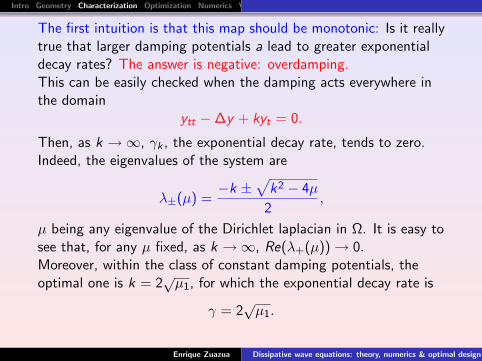
The first intuition is that this map should be monotonic: Is it reallytrue that larger damping potentials a lead to greater exponentialdecay rates? The answer is negative: overdamping.This can be easily checked when the damping acts everywhere inthe domain
ytt −∆y + kyt = 0.
Then, as k →∞, γk , the exponential decay rate, tends to zero.Indeed, the eigenvalues of the system are
λ±(µ) =−k ±
√k2 − 4µ
2,
µ being any eigenvalue of the Dirichlet laplacian in Ω. It is easy tosee that, for any µ fixed, as k →∞, Re(λ+(µ)) → 0.Moreover, within the class of constant damping potentials, theoptimal one is k = 2
õ1, for which the exponential decay rate is
γ = 2√
µ1.
Enrique Zuazua Dissipative wave equations: theory, numerics & optimal design

Intro Geometry Characterization Optimization Numerics Viscoity
The first intuition is that this map should be monotonic: Is it reallytrue that larger damping potentials a lead to greater exponentialdecay rates? The answer is negative: overdamping.This can be easily checked when the damping acts everywhere inthe domain
ytt −∆y + kyt = 0.
Then, as k →∞, γk , the exponential decay rate, tends to zero.Indeed, the eigenvalues of the system are
λ±(µ) =−k ±
√k2 − 4µ
2,
µ being any eigenvalue of the Dirichlet laplacian in Ω. It is easy tosee that, for any µ fixed, as k →∞, Re(λ+(µ)) → 0.Moreover, within the class of constant damping potentials, theoptimal one is k = 2
õ1, for which the exponential decay rate is
γ = 2√
µ1.
Enrique Zuazua Dissipative wave equations: theory, numerics & optimal design

Intro Geometry Characterization Optimization Numerics Viscoity
Enrique Zuazua Dissipative wave equations: theory, numerics & optimal design
Intro Geometry Characterization Optimization Numerics Viscoity
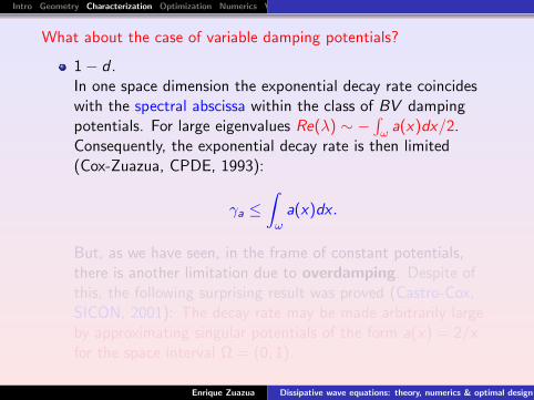
What about the case of variable damping potentials?
1− d .In one space dimension the exponential decay rate coincideswith the spectral abscissa within the class of BV dampingpotentials. For large eigenvalues Re(λ) ∼ −
∫ω a(x)dx/2.
Consequently, the exponential decay rate is then limited(Cox-Zuazua, CPDE, 1993):
γa ≤∫
ωa(x)dx .
But, as we have seen, in the frame of constant potentials,there is another limitation due to overdamping. Despite ofthis, the following surprising result was proved (Castro-Cox,SICON, 2001): The decay rate may be made arbitrarily largeby approximating singular potentials of the form a(x) = 2/xfor the space interval Ω = (0, 1).
Enrique Zuazua Dissipative wave equations: theory, numerics & optimal design

Intro Geometry Characterization Optimization Numerics Viscoity
This potential plays the role of transparent boundary conditions forwhich solutions achieve the equilibrium in finite time:
ytt − yxx = 0 in (0, 1)× (0,∞)y = 0 at x = 1, t ≥ 0yx − yt = 0 at x = 0, t ≥ 0y(x , 0) = y0(x), yt(x , 0) = y1(x) in (0, 1),
In this case:y ≡ 0, for t ≥ 2,
and the exponential decay rate is arbitrarily large.
Enrique Zuazua Dissipative wave equations: theory, numerics & optimal design

Intro Geometry Characterization Optimization Numerics Viscoity
In the multidimensional case the situation is even more complex.In this case it is not longer true that the spectral absicssacharacterizes the exponential decay rate. There are actually twoquantities that enter in such characterization (G. Lebeau, 1996):
The spectral abscissa;
The minimum asymptotic average (as T →∞) of thedamping potential along rays of Geometric Optics.The later is in agreement with the intuition we gain throughthe analysis of the GCC: If a ray escapes the damping regionthe exponential decay property fails. Similarly, if a ray staysfor a very short time interval within the decay region, then thedissipative mechanism is very weak on the solutions localizedon it.
Enrique Zuazua Dissipative wave equations: theory, numerics & optimal design

Intro Geometry Characterization Optimization Numerics Viscoity
This is a typical situation in which the spectral abscissa does notsuffice to capture the decay rate. The damping mechanism isactive on the outer neighborhood of the exterior boundary. Whenthe domain is the ellipsoid this produces the exponential decay.But, in the presence of the two holes, the exponential decay rate islost, due to the existence of a trapped ray that never meets thedamping region. In this case the decay rate is zero but thespectrum is not essentially affected if the holes are small enough.Thus the spectrum is unable to characterize the null decay rate.
Enrique Zuazua Dissipative wave equations: theory, numerics & optimal design

Intro Geometry Characterization Optimization Numerics Viscoity
The optimal design of the damping potential with constraints(size, shape, etc.) is still widely open.
Hebrard-Henrot, SCL, (2003) show the complexity of theproblem in the 1− d case for small amplitude dampingpotentials located on the union of a finite number of intervals.Hebrard-Humbert, 2003): Optimization of the shape of ω in asquare domain in view of the geometric optics quantityentering in the characterization of the decay rate.Cox-Henrot, Ammari-Tucsnak, 2002: 1− d problems withdamping terms located at a single point through a Diracdelta. Eigenvalues are complex valued, and they depend bothon the amplitude of the damping and the diophantineproperties of the point support.A. Munch, 2005-2006: Numerical simulation of the optimalshape in multi-dimensional problems using level set methods.Asch-Lebeau, 20033 Numerical approximation using two-gridmethods for capturing propagation along rays.
3M. Asch, G. Lebeau, The spectrum of the damped wave operator forgeometrically complex domain in R2, Experimental Mathematics 12(2) (2003).
Enrique Zuazua Dissipative wave equations: theory, numerics & optimal design
Intro Geometry Characterization Optimization Numerics Viscoity
The optimal design of the damping potential with constraints(size, shape, etc.) is still widely open.
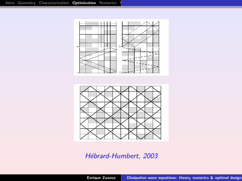
Hebrard-Henrot, SCL, (2003) show the complexity of theproblem in the 1− d case for small amplitude dampingpotentials located on the union of a finite number of intervals.Hebrard-Humbert, 2003): Optimization of the shape of ω in asquare domain in view of the geometric optics quantityentering in the characterization of the decay rate.Cox-Henrot, Ammari-Tucsnak, 2002: 1− d problems withdamping terms located at a single point through a Diracdelta. Eigenvalues are complex valued, and they depend bothon the amplitude of the damping and the diophantineproperties of the point support.A. Munch, 2005-2006: Numerical simulation of the optimalshape in multi-dimensional problems using level set methods.Asch-Lebeau, 20033 Numerical approximation using two-gridmethods for capturing propagation along rays.
3M. Asch, G. Lebeau, The spectrum of the damped wave operator forgeometrically complex domain in R2, Experimental Mathematics 12(2) (2003).
Enrique Zuazua Dissipative wave equations: theory, numerics & optimal design
Intro Geometry Characterization Optimization Numerics Viscoity
Hebrard-Humbert, 2003
Enrique Zuazua Dissipative wave equations: theory, numerics & optimal design

Intro Geometry Characterization Optimization Numerics Viscoity
A. Munch, 2005.
Enrique Zuazua Dissipative wave equations: theory, numerics & optimal design
Intro Geometry Characterization Optimization Numerics Viscoity
The main difficulties are related to the fact that there is novariational principle characterizing the decay rate, and to thecomplex way in which the eigenvalues depend on the dampingpotentials, and the different way they do it forlow/high/intermediate frequencies, for small/large amplitudes ofthe damping potentials, with respect to the shape of the support,....Futhermore, not always all authors deal with the same problem.For instance, the optimal damping for a given initial datum maydiffer significantly from the optimal damping when consideringglobally all possible solutions...This is the case even for constant damping potentials k. Theoptimal damping for the `-th eigenfunction is k = 2
õ`.
Enrique Zuazua Dissipative wave equations: theory, numerics & optimal design

Intro Geometry Characterization Optimization Numerics Viscoity
A different way of formulating the problem of the optimal damperconsists in considering the total energy accumulated by thesolutions for all 0 < t < ∞, i. e. the quantity
F (y0, y1) =
∫ ∞
0E (t)dt.
We can then measure the efficiency of the dasmper in terms of
e(a) = maxE(y0,y1)≤1
F (y0, y1).
The problem can be also formulated in terms of this function e(a).How does the function a → e(a) behave? What is the minimizer ofe(a) in a given class of potentials a?Similar issues can be raised in what concerns the dependence onthe damping region.
Enrique Zuazua Dissipative wave equations: theory, numerics & optimal design
Intro Geometry Characterization Optimization Numerics Viscoity
A closely related problem that has been also investigated is that inwhich the damping potential changes sign. It is natural to analyzewhether the exponential decay property holds for potentials withpositive average.The situation is quite complex. The following results are known:
For damping potentials ka with k large and a changing signthere exist eigenfunctions for which the eigenvalue is real andpositive. Thus, the system becomes unstable. 4
For εa with ε small enough, in one space dimension, theexponential decay property holds if and only if the followinginequalities are satisfied:∫
a(x)φk(x)dx > 0,
for all eigenfunction of the Dirichlet Laplacian φk . Thisassumption is much stronger than simply assuming that theaverage of a is positive. 5
4J. Lopez-Gomez, JDE.5P. Freitas & E. Z. Stability results for the wave equation with indefinite
damping. J. Diff. Equations., 132 (2) (1996), 338-352.Enrique Zuazua Dissipative wave equations: theory, numerics & optimal design

Intro Geometry Characterization Optimization Numerics Viscoity
The extension of the decay result for small amplitude potentials toseveral space dimensions is an open problem. According thecharacterization above on the decay rate it is also natural toassume that the average of the potential along all rays ofgeometric optics is positive.
Enrique Zuazua Dissipative wave equations: theory, numerics & optimal design

Intro Geometry Characterization Optimization Numerics Viscoity
From a numerical point of view it is natural to address thefollowing issues:
To develop numerical schemes that reproduce the same decayproperties of the original PDE;
To analyze optimal design problems at the numerical level andsee if the numerical optimal designs converge as the mesh-sizetends to zero to the continuous optimal design.
Enrique Zuazua Dissipative wave equations: theory, numerics & optimal design

Intro Geometry Characterization Optimization Numerics Viscoity
Let us analyze the finite difference semi-discrete approximation ofthe 1− d wave equation:
y ′′j −1h2 [yj+1 + yj−1 − 2yj ] + aj1ωh
y ′j = 0, t > 0, j = 1, . . . ,N
yj(t) = 0, j = 0, N + 1, t > 0yj(0) = ϕ0
j , y ′j (0) = ϕ1j , j = 1, . . . ,N.
Here h = 1/(N + 1) > 0 and consider the meshx0 = 0 < x1 < ... < xj = jh < xN = 1− h < xN+1 = 1, whichdivides [0, 1] into N + 1 subintervals Ij = [xj , xj+1], j = 0, ...,N.
Enrique Zuazua Dissipative wave equations: theory, numerics & optimal design

Intro Geometry Characterization Optimization Numerics Viscoity
Enrique Zuazua Dissipative wave equations: theory, numerics & optimal design
Intro Geometry Characterization Optimization Numerics Viscoity
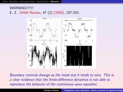
WARNING!!!!!!E. Z., SIAM Review, 47 (2) (2005), 197-243.
Boundary controls diverge as the mesh size h tends to zero. This isa clear evidence that the finite-difference dynamics is not able toreproduce the behavior of the continuous wave equation.
Enrique Zuazua Dissipative wave equations: theory, numerics & optimal design
Intro Geometry Characterization Optimization Numerics Viscoity
WHY?
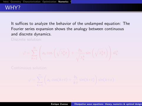
It suffices to analyze the behavior of the undamped equation: TheFourier series expansion shows the analogy between continuousand discrete dynamics.Discrete solution:
~ϕ =N∑
k=1
ak cos
(√λh
kt
)+
bk√λh
k
sin
(√λh
kt
) ~whk .
Continuous solution:
ϕ =∞∑
k=1
(ak cos(kπt) +
bk
kπsin(kπt)
)sin(kπx)
Enrique Zuazua Dissipative wave equations: theory, numerics & optimal design

Intro Geometry Characterization Optimization Numerics Viscoity
WHY?
It suffices to analyze the behavior of the undamped equation: TheFourier series expansion shows the analogy between continuousand discrete dynamics.Discrete solution:
~ϕ =N∑
k=1
ak cos
(√λh
kt
)+
bk√λh
k
sin
(√λh
kt
) ~whk .
Continuous solution:
ϕ =∞∑
k=1
(ak cos(kπt) +
bk
kπsin(kπt)
)sin(kπx)
Enrique Zuazua Dissipative wave equations: theory, numerics & optimal design

Intro Geometry Characterization Optimization Numerics Viscoity
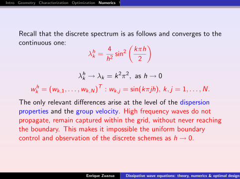
Recall that the discrete spectrum is as follows and converges to thecontinuous one:
λhk =
4
h2sin2
(kπh
2
)λh
k → λk = k2π2, as h → 0
whk = (wk,1, . . . ,wk,N)T : wk,j = sin(kπjh), k, j = 1, . . . ,N.
The only relevant differences arise at the level of the dispersionproperties and the group velocity. High frequency waves do notpropagate, remain captured within the grid, without never reachingthe boundary. This makes it impossible the uniform boundarycontrol and observation of the discrete schemes as h → 0.
Enrique Zuazua Dissipative wave equations: theory, numerics & optimal design
Intro Geometry Characterization Optimization Numerics Viscoity
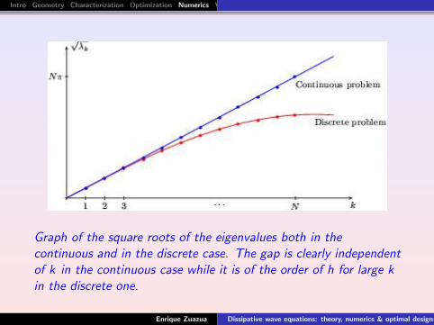
Graph of the square roots of the eigenvalues both in thecontinuous and in the discrete case. The gap is clearly independentof k in the continuous case while it is of the order of h for large kin the discrete one.
Enrique Zuazua Dissipative wave equations: theory, numerics & optimal design
Intro Geometry Characterization Optimization Numerics Viscoity
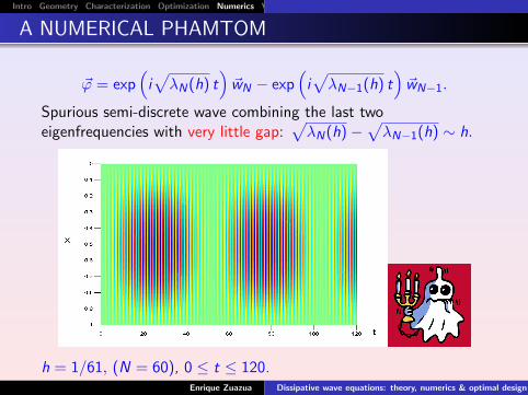
A NUMERICAL PHAMTOM
~ϕ = exp(i√
λN(h) t)
~wN − exp(i√
λN−1(h) t)
~wN−1.
Spurious semi-discrete wave combining the last twoeigenfrequencies with very little gap:
√λN(h)−
√λN−1(h) ∼ h.
h = 1/61, (N = 60), 0 ≤ t ≤ 120.Enrique Zuazua Dissipative wave equations: theory, numerics & optimal design

Intro Geometry Characterization Optimization Numerics Viscoity
Semi-discrete spectrum with N = 200 nodes and dampingcoefficients 2.10−1, 2, 10 and 20 on the interval (1/2, 1).
Enrique Zuazua Dissipative wave equations: theory, numerics & optimal design

Intro Geometry Characterization Optimization Numerics Viscoity
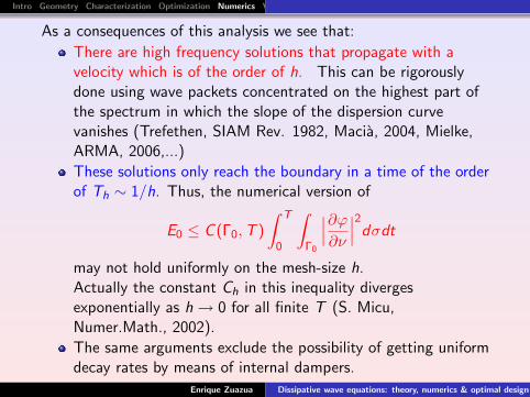
As a consequences of this analysis we see that:
There are high frequency solutions that propagate with avelocity which is of the order of h. This can be rigorouslydone using wave packets concentrated on the highest part ofthe spectrum in which the slope of the dispersion curvevanishes (Trefethen, SIAM Rev. 1982, Macia, 2004, Mielke,ARMA, 2006,...)
These solutions only reach the boundary in a time of the orderof Th ∼ 1/h. Thus, the numerical version of
E0 ≤ C (Γ0,T )
∫ T
0
∫Γ0
∣∣∣∂ϕ
∂ν
∣∣∣2dσdt
may not hold uniformly on the mesh-size h.Actually the constant Ch in this inequality divergesexponentially as h → 0 for all finite T (S. Micu,Numer.Math., 2002).
The same arguments exclude the possibility of getting uniformdecay rates by means of internal dampers.
Enrique Zuazua Dissipative wave equations: theory, numerics & optimal design

Intro Geometry Characterization Optimization Numerics Viscoity
As a consequences of this analysis we see that:
There are high frequency solutions that propagate with avelocity which is of the order of h. This can be rigorouslydone using wave packets concentrated on the highest part ofthe spectrum in which the slope of the dispersion curvevanishes (Trefethen, SIAM Rev. 1982, Macia, 2004, Mielke,ARMA, 2006,...)
These solutions only reach the boundary in a time of the orderof Th ∼ 1/h. Thus, the numerical version of
E0 ≤ C (Γ0,T )
∫ T
0
∫Γ0
∣∣∣∂ϕ
∂ν
∣∣∣2dσdt
may not hold uniformly on the mesh-size h.Actually the constant Ch in this inequality divergesexponentially as h → 0 for all finite T (S. Micu,Numer.Math., 2002).
The same arguments exclude the possibility of getting uniformdecay rates by means of internal dampers.
Enrique Zuazua Dissipative wave equations: theory, numerics & optimal design

Intro Geometry Characterization Optimization Numerics Viscoity
In view of this one may expect a very different behavior of theoptimal design problem in the numerical and the continuouslevel. This has been observed and proved by Hebrard-Henrot,SICON, 2005.
Note that, in view of the dispersion diagram, even whenexcluding the highest frequencies, one observes the existenceof lots of numerical solutions for which the velocity ofpropagation is not the same as for the continuous waveeqation. Numerically the velocity of propagation can be 1/2,1/4, 1/8,... depending on the points of the dispersion diagramin which the wave packets are concentrated.This indicates that the decay rate, that depends on the timespent by characteristic rays on the damping region, willnecessarily differ significantly form that of the continuouswave equation.
Enrique Zuazua Dissipative wave equations: theory, numerics & optimal design

Intro Geometry Characterization Optimization Numerics Viscoity
WELL KNOWN PHENOMENA FOR WAVES IN HIGHLYOSCILLATORY MEDIA
ϕtt − (α(x)ϕx)x = 0.
Enrique Zuazua Dissipative wave equations: theory, numerics & optimal design
Intro Geometry Characterization Optimization Numerics Viscoity
F. Colombini & S. Spagnolo, Ann. Sci. ENS, 1989
M. Avellaneda, C. Bardos & J. Rauch, Asymptotic Analysis,1992.
C. Castro & E. Z. Archive Rational Mechanics and Analysis,2002.
Enrique Zuazua Dissipative wave equations: theory, numerics & optimal design

Intro Geometry Characterization Optimization Numerics Viscoity
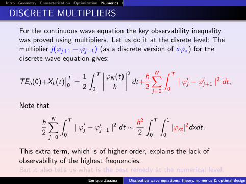
DISCRETE MULTIPLIERS
For the continuous wave equation the key observability inequalitywas proved using multipliers. Let us do it at the disrete level: Themultiplier j(ϕj+1 − ϕj−1) (as a discrete version of xϕx) for thediscrete wave equation gives:
TEh(0)+Xh(t)∣∣T0
=1
2
∫ T
0
∣∣∣∣ϕN(t)
h
∣∣∣∣2 dt+h
2
N∑j=0
∫ T
0| ϕ′j − ϕ′j+1 |2 dt,
Note that
h
2
N∑j=0
∫ T
0| ϕ′j − ϕ′j+1 |2 dt ∼ h2
2
∫ T
0
∫ 1
0|ϕxt |2dxdt.
This extra term, which is of higher order, explains the lack ofobservability of the highest frequencies.But it also tells us what is the best remedy at the numerical level.
Enrique Zuazua Dissipative wave equations: theory, numerics & optimal design

Intro Geometry Characterization Optimization Numerics Viscoity
DISCRETE MULTIPLIERS
For the continuous wave equation the key observability inequalitywas proved using multipliers. Let us do it at the disrete level: Themultiplier j(ϕj+1 − ϕj−1) (as a discrete version of xϕx) for thediscrete wave equation gives:
TEh(0)+Xh(t)∣∣T0
=1
2
∫ T
0
∣∣∣∣ϕN(t)
h
∣∣∣∣2 dt+h
2
N∑j=0
∫ T
0| ϕ′j − ϕ′j+1 |2 dt,
Note that
h
2
N∑j=0
∫ T
0| ϕ′j − ϕ′j+1 |2 dt ∼ h2
2
∫ T
0
∫ 1
0|ϕxt |2dxdt.
This extra term, which is of higher order, explains the lack ofobservability of the highest frequencies.But it also tells us what is the best remedy at the numerical level.
Enrique Zuazua Dissipative wave equations: theory, numerics & optimal design

Intro Geometry Characterization Optimization Numerics Viscoity
Recall that at the continuous level we got
E0 = limT→∞
1
2T
∫ T
0
∫Γ((x − x0) · ν)
∣∣∣∂ϕ
∂ν
∣∣∣2dΓdt.
However, at the discrete level the corresponding identity is:
Eh(0) = limT→∞
1
2T
∫ T
0
∣∣∣∣ϕN(t)
h
∣∣∣∣2 dt+h
2
N∑j=0
∫ T
0| ϕ′j − ϕ′j+1 |2 dt.
Enrique Zuazua Dissipative wave equations: theory, numerics & optimal design

Intro Geometry Characterization Optimization Numerics Viscoity
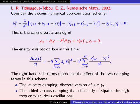
L. R. Tcheugoue-Tebou, E. Z., Numerische Math., 2003.Consider the viscous numerical approximation scheme:
y ′′j −1
h2[yj+1 + yj−1 − 2yj ]−
[y ′j+1 + y ′j−1 − 2y ′j
]+ aj1ωh
y ′j = 0.
This is the semi-discrete analog of
ytt −∆y − h2∆yt + a(x)1ωyt = 0.
The energy dissipation law is this time:
dEh(t)
dt= −h
∑j∈ωh
aj |y ′j |2 − h3N∑
j=0
|y ′j+1 − y ′j |2
h2.
The right hand side terms reproduce the effect of the two dampingterms in this scheme:
The velocity damping, discrete version of a(x)yt ;
The added viscous damping that efficiently dissipates the highfrequency spurious oscillations.
Enrique Zuazua Dissipative wave equations: theory, numerics & optimal design

Intro Geometry Characterization Optimization Numerics Viscoity
L. R. Tcheugoue-Tebou, E. Z., Numerische Math., 2003.Consider the viscous numerical approximation scheme:
y ′′j −1
h2[yj+1 + yj−1 − 2yj ]−
[y ′j+1 + y ′j−1 − 2y ′j
]+ aj1ωh
y ′j = 0.
This is the semi-discrete analog of
ytt −∆y − h2∆yt + a(x)1ωyt = 0.
The energy dissipation law is this time:
dEh(t)
dt= −h
∑j∈ωh
aj |y ′j |2 − h3N∑
j=0
|y ′j+1 − y ′j |2
h2.
The right hand side terms reproduce the effect of the two dampingterms in this scheme:
The velocity damping, discrete version of a(x)yt ;
The added viscous damping that efficiently dissipates the highfrequency spurious oscillations.
Enrique Zuazua Dissipative wave equations: theory, numerics & optimal design

Intro Geometry Characterization Optimization Numerics Viscoity
Theorem: The decay rate of this viscous numerical scheme isuniform, independent of h. Furthermore, the scheme converges (oforder 2) in the classical sense of numerical analysis.This result has been later extended in various ways:
The 1− d wave equation with boundary damping (L. R.Tcheugoue-Tebou, E. Z. 2003);
Multi-dimensional problems (A. Munch-A. Pazoto.ESAIM:COCV, to appear.)
More general 1− d problems (with stronger numericalviscosity, and, therefore, with schemes which are not longer oforder two), M. Tucsnak et al., 2004.
Enrique Zuazua Dissipative wave equations: theory, numerics & optimal design

Intro Geometry Characterization Optimization Numerics Viscoity
But a complete theory is to be developed. The topics to beaddressed include:
More general methods, including the finite element method onirregular meshes;
The obtention, at the discrete level, sharp geometricconditions as the GCC;
Wave equations with variable coefficients;
Other models and systems: plate, beam and shell equations,Schrodinger, elasticity, Maxwell,...
Enrique Zuazua Dissipative wave equations: theory, numerics & optimal design

Intro Geometry Characterization Optimization Numerics Viscoity
But, even in the context of the constant coefficient wave equation,and with the finite-difference semi-discrete scheme above, severalissues are still to be clarified:
How to characterize the optimal decay rate. Can the resultson the continuous wave equation be extended? The notion ofbicharacteristic ray can be adapted to the present setting. Butthe damping is now made of two pieces: The discrete versionof the velocity damping, and the viscous damping actingeverywhere on the domain.
Does the decay rate of the semi-discrete viscous schemeconverge to the one of the continuous wave equation?Even though this scheme provides a uniform exponentialdecay, it is unclear whether it yields the same rate of decay ash → 0. Consequently, it is also highly unclear whether optimaldampers will converge as h → 0. This is an interesting topicfor further investigation.
Enrique Zuazua Dissipative wave equations: theory, numerics & optimal design

Intro Geometry Characterization Optimization Numerics Viscoity
The possible consequences of this type of result in connectionwith the convergence of numerical optimal dampers towardscontinuous ones are also to be developed.
Closely related also to other qualitative properties such asattractors, inertial manifolds, transversality,... (G. Raugel, R.Joly).
This topic is closely linked with the theory of transparentboundary conditions and Perfectly Matching Layers (PML).Work in this direction, inspired in the ides presented here, isbeing developed: S. Ervedoza & E. Z.Note however that, in this case, the wave equation has to bewritten as a system of two equations of first order and thatthe damping term has to be added in both equations. In thisway one gets a dissipative wave equation with a dispersiveterm for which overdamping phenomena do not occur.
Enrique Zuazua Dissipative wave equations: theory, numerics & optimal design