dissertaÇÃo de mestrado -...
TRANSCRIPT

DISSERTAÇÃO DE MESTRADO
Channel modeling for Through-The-Earth(TTE) Communication Systems
Josua Daniel Pena Carreno
Brasília, Fevereiro de 2016
UNIVERSIDADE DE BRASÍLIA
FACULDADE DE TECNOLOGIA


To Ana and Jonathan for supporting me every day of my live
Josua Daniel Pena Carreno

ACKNOWLEDGEMENTS
I would like to thank:Judson Braga for being a good teacher and a strict leaderSavio Neves, Lucas Sousa e Silva and Henrique Berilli for always keeping a positiveattitude and being excellent colleagues.Professors Andre Noll and Leonardo Aguayo, for always having a constructive criticand giving good ideas to solve problemsFelipe Duerno for teaching me new programming languages and helping me out withall simulationsJosé Pereira Filho, Boanerges Ribeiro, Márcio Sales and Leandro Machado for beingbeside me in one of the hardest experiences of my lifeAndré Vieira, Guilherme Santos, Jesús Gonzalez, Johanel Da Silva, Karla Bocaranda,Laila Wanick, Linniker Corado, Luciano Grossi, Pauli Ramirez, Reni Santos, SinamaicaHenriquez, Sirius Bocaranda, and Uirá Godoi for maintaining our friendship all theseyears no matter what distance is between usProfessor Gladys Bruzual, for supporting me since the first day at Engineering SchoolGustavo Sandri, je suis très heureux de t’avoir comme mon ami et professeur particulierde françaisArthur Sudre, for upholding me even without understanding my workAnd my grandmother and my father for taking care of me from heaven.Special thanks to: "Instituto Tecnológico Vale" (ITV) and "Coordenação de Aperfeiçoa-mento de Pessoal de Nível Superior" (CAPES) for supporting this study.
Josua Daniel Pena Carreno

RESUMO
Este trabalho apresenta modelagem de canal em ambientes de comunicação TTE a partir demodelos analíticos estabelecidos, medidas e simulações eletromagnéticas. Para estes cenários,apresenta-se como contribuição original os resultados estatísticos tanto para a condutividadeelétrica efetiva quanto para a atenuação sofrida pelo campo magnético durante a propagação. Osresultados de simulação obtidos aqui, além de confirmarem o comportamento do canal empírico,extrapolam para frequências não estudadas via ferramentas estatísticas.
ABSTRACT
This dissertation presents channel modeling in TTE communication environments from well-established analytic models, measurements and electromagnetic simulations. For those scenarios,the main original contribution are the statistical results for the effective electric conductivity aswell as the attenuation experimented by magnetic field while propagating Through-The-Earth.The simulation results present here, in addition to confirming the behavior of empirical models,extrapolate to frequencies not studied via statistical tools.

RESUMO ESTENDIDO
A comunicação com e entre operários que trabalham em espaços confinados sempre foi temade vital importância para a indústria da mineração, devido a que através de sistemas de comuni-cação pode se manter contato em tempo real com todos os membros das equipes e transferir infor-mações de apoio durante casos de emergência. Mais recentemente, com a crescente automaçãona mineração, também é importante se garantir a comunicação entre os diferentes equipamentose a superfície, Existem vários sistemas de comunicação disponíveis em minas subterrâneas domundo, sendo que, sistemas baseados em cabos coaxiais ou fibra ótica são os mais utilizados.Porém estes não são eficientes em casos de desastre, podendo sofrer quebras e isolar os operários[1], como em explosões, incêndios, inundações e soterramentos, além de serem pouco flexíveisem ambientes cuja topologia muda o tempo todo.
A grande maioria dos sistemas de comunicação sem fio utiliza topologias de comunicaçãoem radiofrequência (RF) baseadas em antenas radiantes, campo distante e meio de transmissãocom características elétricas próximas as do vácuo. No caso em que rochas, solo, água e outrosmateriais de condutividade elétrica não desprezível se tornam o meio de propagação entre aspontas de comunicação, a alta taxa de atenuação de ondas eletromagnéticas em altas frequênciasnão permite o uso desses sistemas acima citados [2].
Comunicações através da terra ou TTE, do inglês, Through-the-earth, consistem no uso de on-das eletromagnéticas para estabelecer um enlace entre a superfície e a mina subterrânea utilizandoa terra como meio de propagação. A transmissão é normalmente feita por indução magnética emfrequências abaixo de 30 kHz, sujeitas a ruídos atmosféricos e a harmônicos produzidos porequipamentos, limitando o desempenho de comunicação, especialmente no enlace de subida [2].
Uma regulamentação do congresso americano exigindo um sistema de comunicação de emergên-cia em minas subterrâneas de carvão que opere em caso de acidentes, chamada lei Mine Improve-ment and New Emergency Response Act (MINER Act), impulsionou a pesquisa e o desenvolvi-mento das comunicações TTE. Segundo a lei, este sistema deve ser sem fio, bidirecional, provercomunicação entre a superfície e o subterrâneo da mina e ser capaz de rastrear as pessoas presasno subterrâneo [3].
Pode-se também utilizar comunicações subterrâneas diferentes do TTE sendo essas cabeadas(TTW, Through-the-wire) e/ou sem fio (TTA, Through-the-air). Entre as possíveis aplicações,pode-se citar: automação das máquinas presentes na mineração; acionamento de explosivos; co-municação entre mineiros por dados ou de voz; monitoramento da mina por vídeo; monitoramentodo estado dos mineiros; detecção de níveis elevados de gases danosos aos mineiros, o monitora-mento e coordenação em tempo real da frota e pessoal.
Neste trabalho apresentamos alguns conceitos sobre comunicações em minas, motivados pelagrande importância da indústria da mineração no Brasil e sua rápida evolução tecnológica, aliada
vii

à pequena produção científica desta área no país. Este trabalho traz uma visão geral sobre estudos,modelos e equipamentos em torno de comunicações subterrâneas.
CONDIÇÕES PARA A COMUNICAÇÃO EM MINAS SUBTERRÂNEAS
Uma mina pode ser definida como uma massa individual de substância mineral ou fóssil, emlavra, esteja ela na superfície terrestre ou no interior da terra e que tenha um valor econômico [4].Geralmente, minas subterrâneas são muito úmidas, com umidade relativa do ar podendo chegara 90% ou mais. Água corrosiva, poeira, gases explosivos e tóxicos, como dióxido de carbono emetano, são substâncias que podem afetar não só o bem estar de operários, mas também a vidaútil e regulagem de equipamentos, incluindo os de comunicação.
Esse cenário guarda algumas semelhanças com a aplicações da construção civil, como túneise metrô, mas com condições mais hostis. Porém, uma característica particular de minas sub-terrâneas é a sua expansão em função da retirada de minério estéril. A expansão do espaço decobertura pode levar à necessidade do aumento da infraestrutura de telecomunicações [5]. Istoé especialmente verdade em comunicações TTA, que tem o ar da mina como meio de propa-gação. Outro aspecto da mina que também influencia as comunicações TTA é a sua forma e tipode acesso. Escavações que formem minas abertas sustentadas por pilares trazem condições depropagação de ondas diferentes daquelas minas em túnel que tendem a criar um efeito de guia deonda com baixo índice de perda de propagação.
Com respeito às características elétricas do meio, minas diferem uma das outras não apenaspelo mineral explorado, mas também pela proporção deste mineral em relação a outros materi-ais, como os que compõem o capeamento (overburden) que separa a superfície do corpo útil deminério. A variação da condutividade elétrica do meio, em função desta proporção, influenciabastante a perda de propagação no canal, e pode definir o tipo de equipamento e configuraçõesescolhidas para o funcionamento de sistemas de comunicação TTE. Para comunicações em rádio-frequência dentro das minas, como em TTA e, em alguns casos, em TTW, a condutividade dasparedes da mina influencia os coeficientes de reflexão e difração e, por consequência, a dispersãotemporal do canal de propagação.
USO, TÉCNICAS E EQUIPAMENTOS
Há três principais categorias de comunicação em minas que se destacam: TTW, TTA e TTE,discutidas a seguir.

TTW: através do cabo
Sistemas de comunicação TTW usam meios guiados [5] tanto para comunicação dentro damina quanto entre superfície e mina. Um dos mais antigos instrumentos para comunicação emminas é o telefone de magneto [6], baseado em linha cabeada para comunicação de voz. Umgerador de magneto composto por ímãs é acionado manualmente por uma alavanca produzindotensão alternada de 100 V entre 15 e 20 Hz, que após sua transmissão pelo cabo aciona os sinosdos outros telefones conectados. Estabelecida a conexão, baterias são usadas para garantir aalimentação dos equipamentos de comunicação de voz.
Fibras ópticas permitem altas taxas de transmissão de dados a grandes distâncias dentro damina podendo chegar até 70 km sem necessidade de regeneração do sinal. Por ser uma ferramentade grande capacidade, é utilizada para monitoramento em tempo real das diversas atividades damina como sistema contra incêndio, sistemas automáticos entre outros [7].
Por sua vez, o leaky feeder é um cabo irradiante híbrido entre a transmissão por cabo (TTW)e a transmissão pelo ar (TTA). Utiliza um cabo coaxial fendido para transmitir e receber a in-formação dentro do túnel. Este cabo, em vez de ter uma malha protetora, possui uma camadade cobre com perfurações que atuam como um arranjo de antenas de abertura. Devido à perdaao longo do cabo, é necessário ter amplificadores regularmente espaçados tipicamente entre 350e 500 m de distância. Os cabos fendidos funcionam em ambas as direções de comunicação,usualmente nas bandas VHF e UHF [8].
TTA: Através do ar
Para comunicação dentro da mina, sistemas sem fio (TTA) se tornam mais vantajosos queTTW pela facilidade de instalação e adaptação à expansão da mina. Nos dias de hoje, os sis-temas de comunicação TTA em minas são, em sua maioria, adaptações de um ou vários sistemasde comunicação sem fio para curto alcance como Zigbee, WiFi, RFID, etc. [9]. Visto que osequipamentos de rádio utilizados não trazem novidades em relação aos dispositivos RF usadosem outras aplicações, esta seção se foca nas propostas de protocolos de redes para comunicaçãoTTA encontradas na literatura.
Considerando a disposição dos nós e a falta de infraestrutura em minas, muitos trabalhosindicam a utilização de redes ad hoc. Um dos fatores investigados é o desempenho de protocolos,principalmente aqueles de controle de acesso ao meio ou de roteamento. Na área dos protocolosde controle de acesso ao meio, pode-se citar [10], o qual realiza uma análise de desempenho doprotocolo MINECOM, baseado em TDMA-TDD (time division multiple access - time divisionduplexing).
Percebe-se que muitos trabalhos partem do pressuposto da utilização de padrões ou tecnolo-gias que especifiquem os protocolos de camadas inferiores, como por exemplo o IEEE 802.15.4ou alguma vertente do IEEE 802.11. Com relação a protocolos de roteamento, Jing [11] desen-volve um protocolo híbrido de roteamento para nós móveis baseados no protocolo GEAR (geo-

graphical and energy aware routing). Neste protocolo, os nós móveis possuem sua comunicaçãorestrita a apenas alguns nós em função da distância e direção de movimento entre eles. Ao serealizar essas restrições, consegue-se aumentar o tempo de vida desses nós móveis.
Em [12, 13, 14], análises do desempenho dos protocolos DSDV (destination-sequenced distance-vector) e AODV(ad hoc on-demand distance vector) são feitas, levando em consideração a taxade perda de pacotes, o atraso fim a fim e a vazão em transmissões de vídeo, enquanto que [15]realiza o estudo da utilização do protocolo OLSR (optimized link state routing) e do padrão IEEE802.11n para prover a transmissão de vídeo e voz em minas. Bons resultados de vazão, latência ejitter da rede são encontrados.
Já em [16], há o desenvolvimento de um protocolo de roteamento multi-hop que utiliza um al-goritmo recursivo entre os nós vizinhos para possibilitar a seleção de um caminho que possua umamenor quantidade de saltos, levando em consideração a métrica RSSI (received signal strengthindicator). Para verificar o protocolo, testes foram realizados utilizando o transmissor MG2455da Radio Pulse. Jiang [17] desenvolve um protocolo de roteamento que leva em consideração adisposição dos túneis em minas, em que há um túnel principal e alguns ramos. Considerando adisposição dos nós e a formação de clusters entre eles nesses túneis-ramos, o autor sugere umaforma de realocamento de nós para cada cluster a fim de equilibrar a rede.
Zheng [18] descreve a disposição de redes de sensores subterrâneas, assim como as difi-culdades existentes no canal sem fio subterrâneo e, por fim, explicita os obstáculos e áreas depesquisas para as camadas de rede, considerando também um desenvolvimento cross-layeredcomo um possível mitigador dos desafios encontrados em redes subterrâneas.
TTE: Através da terra
Nos anos que seguiram o MINER Act, o NIOSH (National Institute for Occupational Safetyand Health) apoiou o desenvolvimento de uma série de tecnologias de comunicação e rastrea-mento em minas subterrâneas [3]. Cinco protótipos foram desenvolvidos por cinco empresas:Alertek, E-Spectrum Technologies, Lockheed Martin, Stolar e Ultra Electronics. Quatro protóti-pos baseiam-se na detecção de campos magnéticos utilizando antenas loop e uma na detecção decampos elétricos.
Os sistemas TTE desenvolvidos se mostraram capazes de prover comunicação unidirecional e,em alguns casos, bidirecional, de voz e texto em até 300 m (voz) e 600 m (texto) de profundidade,aproximadamente. Para transmitir voz, os protótipos utilizaram frequências de 3150 Hz a 4820Hz. Alguns protótipos possuíam também um modo de localização baseado em triangulação,em que apenas um tom é transmitido no enlace de subida. Utilizando receptores dispostos nasuperfície é possível localizar a posição do transmissor por meio do tratamento do sinal recebido.
Utilizou-se em alguns protótipos modulação analógica SSB (single side band), e em outrosmodulação digital PSK (phase shift keying) e/ou FSK (frequency shift keying). Além disso, emalguns protótipos, técnicas de cancelamento de ruído foram testadas [3]. Algumas empresas

conseguiram transformar seus projetos em produtos comerciais [19].
O Flex Alert, fabricado pela canadense Mine-Radio Systems, é um sistema de comunicaçãounidirecional entre galerias subterrâneas e a superfície, utilizado para dar suporte na evacuação deoperários em caso de emergência. Utiliza um campo magnético a baixa frequência que transportainformação a um receptor posicionado no capacete dos mineiros. É composto por uma antenatipo loop de 10 a 120 m de comprimento posicionada estrategicamente sobre a mina. Quando háalguma emergência, um sinal é emitido da superfície para todos os mineiros fazendo a lâmpadado capacete piscar sinalizando a evacuação [7].
O Dispositivo Pessoal de Emergência (PED) da australiana MineSite Technology é um sis-tema de comunicação unidirecional que permite a transmissão de mensagens de texto específicasàs pessoas que se encontram no interior da mina sem uso de cabos. Mesmo fornecendo comuni-cação só superfície-mina, pode ser utilizado um cabo irradiante (leaky feeder) para completar acomunicação no link de subida [7]. O sistema também é usado para detonação remota de explo-sivos e controle remoto de equipamentos.
Após seus testes em conjunto com a NIOSH, a Lockheed Martin comercializa a MagneLinkMCS, que é um sistema TTE autossuficiente e bidirecional que oferece suporte a voz, texto elocalização baseado em ondas magnéticas de baixa frequência. Testes a 500 metros de profundi-dade validaram as aplicações de voz e texto, em que uma antena de 130 metros de comprimentoe outra com múltiplas voltas foram usadas na superfície e na mina, respectivamente.
A canadense Vital Alert [20] desenvolveu recentemente o sistema digital Canary de rádio TTEbidirecional para comunicação de dados e voz. O receptor da Canary é implementado em rádiodefinido por software, sendo facilmente reconfigurável para operar entre frequências de 300 Hz a9 kHz. O dispositivo permite modulação adaptativa com taxas que variam de 9 bps a 1 kbps.
Em se tratando de processamento de sinais, [2] sugere o uso de modulação MSK (minimumshift keying). O autor também sugere técnicas de combate ao ruído atmosférico e de códigoscorretores de erros, para conferir maior robustez ao sistema. O autor afirma melhorar a razãosinal-ruído (RSR) de 10 a 30 dB após a caracterização do ruído utilizando múltiplas antenas or-togonais e a aplicação de técnicas como cancelamento adaptativo de ruído, detecção por máximaverossimilhança e realimentação de decisão. A falta de estudos mais recentes em processamentode sinais para comunicação TTE pode indicar que ainda exista um ganho de desempenho a seralcançado via tratamento de sinais em investigações futuras.
PROPAGAÇÃO EM COMUNICAÇÃO TTE
O modo de transmissão TTE mais promissor é ilustrado na Figura 1, onde antenas loop nasuperfície e no subsolo trocam informação via indução magnética. As dimensões e massa de cadauma das antenas, corrente de excitação e frequência de operação definem a qualidade e alcance detransmissão, e podem variar de acordo com o objetivo do sistema, profundidade e características

do solo [21].
Ar: µ0,ǫ0
Meio condutor 1: σ1
Meio condutor 2: σ2
H
Antena loop no subsolo
Figure 1: Representação esquemática de sistema de comunicação TTE, operando em downlink. As dimensões típicasdas antenas são da ordem de dezenas de metros.
Devido às propriedades intrínsecas do solo, a penetração de ondas de rádio em meio con-dutor obedece à equação de difusão ∇2H = µσ∂H/∂t, em vez da equação de onda ∇2H =
µε(∂2H)/(∂t2) com o campo decaindo exponencialmente em função da distância percorrida, fre-quência de operação e condutividade elétrica do meio. O grau de decaimento é frequentementeassociado à função da profundidade pelicular δ =
√2/(ωµσ), que representa a distância na qual
a intensidade de uma onda plana reduz a 1/e de seu valor. Ou seja, a taxa de decaimento emfunção da distância x é expressa por e−x/δ. Portanto, a profundidade pelicular é inversamenteproporcional à raiz quadrada da frequência, o que justifica o uso de frequências baixas, usual-mente abaixo de 30kHz, para comunicação TTE. Essas observações são verdadeiras para meiobom condutor. [22] considera um bom condutor todo material que satisfaça σ/(εω) >> 1.
Para irradiar ondas eletromagnéticas em frequências tão baixas, as antenas deveriam ser quilo-métricas para entrarem em ressonância. Em comunicação TTE, a transferência de potência reativavia indução magnética (ou elétrica) corresponde à quase totalidade da potência transmitida. Apropagação em meio condutor ou dielétrico também altera algumas propriedades básicas da onda,como a velocidade de propagação vrocha e o comprimento de onda λrocha. Em um bom condutor,a contribuição da permissividade real pode ser desprezada e o comprimento de onda que atravessaas rochas da mina pode ser escrito como λrocha = 2πδ, o que em comunicação TTE operandoa 10 kHz com σ = 10−3S/m pode reduzir em 30 vezes o comprimento de onda em relação aoar. Desta forma, afirmar que comunicação TTE sempre ocorre em campo próximo pode não sercorreto.
Zonas de Campo
Classicamente, as zonas de campo para transmissão no vácuo ou no ar são divididas em campopróximo reativo, campo próximo radiante, zona de transição e campo distante [23]. Nas duas

primeiras zonas, o campo é resultado da interferência de ondas de diversos pontos da antena, comose fossem vários pequenos dipolos contribuindo na formação do campo. Em campo distante, ondeos campos elétrico e magnético estão em fase e possuem uma relação fixa entre si, a antena detransmissão é vista como um ponto radiante e seu campo pode ser visto como uma frente de ondaplana. Na zona de transição, ambos os comportamentos podem ser observados. Em um meiocondutor, Gibson [22] propôs uma subdivisão diferente para as zonas de campo.
Em regiões muito próximas à antena de transmissão, o campo possui uma natureza quase-estática seguindo leis da estática como a atenuação pelo inverso do cubo da distância, apesar davariação no tempo. A partir do chamado campo próximo, onde, assim como em quase-estático,inexiste irradiação, o meio condutor começa a contribuir em atenuação de campo. Na zona decampo distante, apesar das perdas devidas ao meio, o campo obedece à lei de atenuação cominverso linear da distância. Campo distante, no caso, não quer dizer que a radiação parte daantena diretamente, e sim pela indução de correntes parasitas [24] no meio condutivo provocadapelo campo magnético da antena, as quais geram novos campos. Por fim, a zona de transição éuma região arbitrária entre os campos próximo e distante.
A Tabela 3.1 traz as zonas de campo e suas condições para dois tipos de meio. Um sistemaoperando no espaço livre a 10 kHz (λ0=30 km) com separação entre antenas de 300 m se encontraem campo próximo reativo (λ0
2π≈ 4775 m), enquanto que em meio condutor com σ = 10−3S/m e
µ = µ0, λrocha2π= δ ≈ 160 m < 300 m. Ou seja, trata-se de zona de transição e está mais próximo
do campo distante do que do campo próximo.
Modelo Tipo de aproximação Condições
Vácuo
Campo próximo reativo r < λ02π
Campo próximo radiante λ02π < r < λ0
Zona de transição λ0 < r < 2λ0Campo distante r > 2λ0 ou 2D2/λ0
Meio condutivo
Quase estático r << λrocha2π
Campo próximo r2 << (λrocha2π )2
Zona de transição r ≈ λrocha2π
Campo distante r >> λrocha2π
Table 1: Zonas de campo no vácuo e em meio condutor
Modelo de Campo Magnético H
O momento magnético de uma antena loop indica a eficiência de transmissão indutiva emfunção das características do transmissor como o número de voltas do loop, a corrente RMS nosfilamentos da antena de transmissão e a área do loop. O aumento de momento magnético tempor custo o aumento da potência dissipada em calor nos filamentos da antenna. A aproximaçãomais simples para o campo magnético variante no tempo gerado por uma antena loop se fazconsiderando o vácuo como meio homogêneo infinito ignorando qualquer condição de contorno[25]. O modelo traz as componentes vertical e horizontal do campo magnético sendo usadas, namaioria das vezes, em comunicação coxial e coplanar entre dois loops, respectivamente, e que

dependem do momento magnético, distância e frequência. A adaptação para um meio infinitocondutivo (MIC) para ambos os enlaces de subida e descida é feita modificando-se apenas onúmero de onda em função da distância pelicular δ. Wait formulou expressões analíticas docampo magnético de antennas circulares com corrente uniforme distinguindo os meios superfíciee subterrâneo, nos chamados modelos de semi-espaço homogêneo (SEH), para os enlaces desubida [26] e de descida [27]. Nestes modelos existe reciprocidade entre os dois enlaces apenaspara o campo vertical, e não o horizontal, diferentemente do modelo MIC. Durkin [28] sugere queexista na interface entre a terra e o ar uma barreira de transposição que possa ser modelada poruma fina camada de condutividade ainda maior que aquela do semi-espaço homogêneo abaixodela. Chamamos este modelo de semi-espaço homogêneo com superfície condutora, em que aespessura da camada de interface e sua condutividade são parâmetros de entrada.

INDEX
1 INTRODUCTION . . . . . . . . . . . . . . . . . . . . . . . . . . . . . . . . . . . . . . . . . . . . . . . . . . . . . . . . . . . . . . 1
2 BASIC CONCEPTS . . . . . . . . . . . . . . . . . . . . . . . . . . . . . . . . . . . . . . . . . . . . . . . . . . . . . . . . . . . . . . 42.1 MINE . . . . . . . . . . . . . . . . . . . . . . . . . . . . . . . . . . . . . . . . . . . . . . . . . . . . . . . . . . . . . . . . . . . . . . . . . . . . 42.2 UNDERGROUND MINE COMMUNICATION . . . . . . . . . . . . . . . . . . . . . . . . . . . . . . . . . . . . 52.2.1 TTW: THROUGH-THE-WIRE . . . . . . . . . . . . . . . . . . . . . . . . . . . . . . . . . . . . . . . . . . . . . . . . . . 52.2.2 TTA: THROUGH-THE-AIR . . . . . . . . . . . . . . . . . . . . . . . . . . . . . . . . . . . . . . . . . . . . . . . . . . . . . 72.3 PROTOCOLS USED FOR UNDERGROUND COMMUNICATION . . . . . . . . . . . . . . . . 82.4 EQUIPMENT FOR UNDERGROUND COMMUNICATION . . . . . . . . . . . . . . . . . . . . . . . . 92.5 NUMERICAL SIMULATIONS OF MAGNETIC TRANSMISSION ENVIRONMENTS 10
3 PROPAGATION IN UNDERGROUND TTE COMMUNICATION SYSTEMS. 123.1 FIELD ZONES . . . . . . . . . . . . . . . . . . . . . . . . . . . . . . . . . . . . . . . . . . . . . . . . . . . . . . . . . . . . . . . . . . . 123.2 ANTENNA MODELING FOR TTE COMMUNICATIONS . . . . . . . . . . . . . . . . . . . . . . . . 133.3 THEORETICAL MODELS FOR TTE PROPAGATION . . . . . . . . . . . . . . . . . . . . . . . . . . 153.3.1 INFINITE CONDUCTIVE MEDIUM (IC) . . . . . . . . . . . . . . . . . . . . . . . . . . . . . . . . . . . . . . . . 153.3.2 HOMOGENEOUS HALF-SPACE MODEL (HHS) . . . . . . . . . . . . . . . . . . . . . . . . . . . . . . 163.3.3 THIN SHEET MODEL (TS) . . . . . . . . . . . . . . . . . . . . . . . . . . . . . . . . . . . . . . . . . . . . . . . . . . . . . 173.3.4 MULTI-LAYER MODEL . . . . . . . . . . . . . . . . . . . . . . . . . . . . . . . . . . . . . . . . . . . . . . . . . . . . . . . . . . 183.4 CHANNEL MODELING AND OPTIMUM OPERATION FREQUENCY . . . . . . . . . . . 203.5 SOIL CONDUCTIVITY . . . . . . . . . . . . . . . . . . . . . . . . . . . . . . . . . . . . . . . . . . . . . . . . . . . . . . . . . . . 23
4 ANALYSIS OF ANALYTIC MODELS, MEASUREMENTS AND SIMULATIONS . . . . . . . . . . 264.1 THEORETICAL MODELS FOR H-FIELD AND TRANSFER FUNCTION . . . . . . . . . 264.1.1 MAGNETIC FIELD . . . . . . . . . . . . . . . . . . . . . . . . . . . . . . . . . . . . . . . . . . . . . . . . . . . . . . . . . . . . . . . 264.1.2 TRANSFER FUNCTION . . . . . . . . . . . . . . . . . . . . . . . . . . . . . . . . . . . . . . . . . . . . . . . . . . . . . . . . . 274.2 HHS AND TS MODELS CURVES . . . . . . . . . . . . . . . . . . . . . . . . . . . . . . . . . . . . . . . . . . . . . . 284.3 PRELIMINARY SIMULATION RESULTS . . . . . . . . . . . . . . . . . . . . . . . . . . . . . . . . . . . . . . . . . 294.3.1 SCENARIO I: FIXED NUMBER OF LAYERS . . . . . . . . . . . . . . . . . . . . . . . . . . . . . . . . . . . . 304.3.2 SCENARIO II: RANDOM NUMBER OF LAYERS . . . . . . . . . . . . . . . . . . . . . . . . . . . . . . . . 314.4 ELECTRIC CONDUCTIVITY CHARACTERIZATION THROUGH MEASUREMENTS
IN UNDERGROUND MINES . . . . . . . . . . . . . . . . . . . . . . . . . . . . . . . . . . . . . . . . . . . . . . . . . . . . . 324.4.1 EQUIVALENT ELECTRIC CONDUCTIVITY OVER ALL FREQUENCIES AND
DEPTHS . . . . . . . . . . . . . . . . . . . . . . . . . . . . . . . . . . . . . . . . . . . . . . . . . . . . . . . . . . . . . . . . . . . . . . . . . 354.4.2 EQUIVALENT ELECTRIC CONDUCTIVITY ESTIMATION AS A FUNCTION OF
FREQUENCY . . . . . . . . . . . . . . . . . . . . . . . . . . . . . . . . . . . . . . . . . . . . . . . . . . . . . . . . . . . . . . . . . . . . 36
xv

4.4.3 EQUIVALENT ELECTRIC CONDUCTIVITY ESTIMATION AS A FUNCTION OF
MINE DEPTH . . . . . . . . . . . . . . . . . . . . . . . . . . . . . . . . . . . . . . . . . . . . . . . . . . . . . . . . . . . . . . . . . . . . 404.5 MULTI-LAYER STATISTICAL MODEL THROUGH ELECTROMAGNETIC FIELD
SIMULATIONS . . . . . . . . . . . . . . . . . . . . . . . . . . . . . . . . . . . . . . . . . . . . . . . . . . . . . . . . . . . . . . . . . . . 424.5.1 H-FIELD VARIATION AS A FUNCTION OF DEPTH AND FREQUENCY . . . . . . . . . 434.5.2 H-FIELD MEDIAN FITTING . . . . . . . . . . . . . . . . . . . . . . . . . . . . . . . . . . . . . . . . . . . . . . . . . . . . . . 454.5.3 EQUIVALENT CONDUCTIVITY . . . . . . . . . . . . . . . . . . . . . . . . . . . . . . . . . . . . . . . . . . . . . . . . . . 474.6 ISSUES SOLVED WHILE USING THE COMMERCIAL SIMULATOR . . . . . . . . . . . . . 50
5 CONCLUSION . . . . . . . . . . . . . . . . . . . . . . . . . . . . . . . . . . . . . . . . . . . . . . . . . . . . . . . . . . . . . . . . 62
BIBLIOGRAPHICAL REFERENCES . . . . . . . . . . . . . . . . . . . . . . . . . . . . . . . . . . . . . . . . . . . . 64
APPENDIX . . . . . . . . . . . . . . . . . . . . . . . . . . . . . . . . . . . . . . . . . . . . . . . . . . . . . . . . . . . . . . . . . . . . . . . . . 68
I MINER ACT OF 2006 . . . . . . . . . . . . . . . . . . . . . . . . . . . . . . . . . . . . . . . . . . . . . . . . . . . . . . . . . . 69
II 3D MAGNETIC FIELD SIMULATION ON CST STUDIO SUITE . . . . . . . . . . . . . . . . . . . . 71
III ROOT MEAN SQUARE ERROR (RMSE) . . . . . . . . . . . . . . . . . . . . . . . . . . . . . . . . . . . . . . . . . . 74
IV LOGNORMAL DISTRIBUTION . . . . . . . . . . . . . . . . . . . . . . . . . . . . . . . . . . . . . . . . . . . . . . . . . . . . 75
V STATISTICAL PARAMETERS USED . . . . . . . . . . . . . . . . . . . . . . . . . . . . . . . . . . . . . . . . . . . . . . . 76
VI NUMERIC METHODS FOR ELECTROMAGNETIC MODELING . . . . . . . . . . . . . . . . . . . . . . . . 78VI.1 FDTD .. . . . . . . . . . . . . . . . . . . . . . . . . . . . . . . . . . . . . . . . . . . . . . . . . . . . . . . . . . . . . . . . . . . . . . . . . . 78VI.2 METHOD OF MOMENTS (MOM) .. . . . . . . . . . . . . . . . . . . . . . . . . . . . . . . . . . . . . . . . . . . . . 79VI.3 FINITE ELEMENT METHOD (FEM) . . . . . . . . . . . . . . . . . . . . . . . . . . . . . . . . . . . . . . . . . . . 80
VII MAGNETIC FIELD MEASUREMENTS FROM 94 AMERICAN COAL MINES . . . . . . . . . . . 83
VIIIH-FIELD STATISTICAL DISTRIBUTIONS FOR FREQUENCY AND DEPTH . . . . . . . . . . . . 89

FIGURE LIST
1 Representação esquemática de sistema de comunicação TTE, operando em down-link. As dimensões típicas das antenas são da ordem de dezenas de metros. .......... xii
2.1 Surface and underground mines .................................................................. 52.2 Magnetic telephone .................................................................................. 62.3 Fiber optics............................................................................................. 62.4 Leaky Feeder .......................................................................................... 72.5 TE and TM modes in waveguides ................................................................ 7
3.1 Through-The-Earth communication ............................................................. 123.2 Field regions for typical Antennae Adapted from: OSHA [29] ........................... 133.3 Channel transfer function........................................................................... 143.4 Infinite Conductive Medium IC ................................................................... 163.5 HHS Geometry........................................................................................ 173.6 Thin sheet configuration ............................................................................ 183.7 Stratified soil for Multi-layer model ............................................................. 193.8 Geometry used in the calculation of the magnetic field between two circular loop
antennae. The angle α formed by orthogonal vectors to the planes determined bythe two antennae is the result of rotations around the x′ e y′ axis. ....................... 21
3.9 Equivalent conductivity for 630 Hz for 94 coal mines ...................................... 243.10 Estimated Apparent conductivities (S/m) change with overburden depth interval
(m) for various σ d at 630 Hz...................................................................... 24
4.1 H-field from a loop antenna for coaxial and co-planar configuration .................... 274.2 Channel transfer function........................................................................... 274.5 H-field TS and HHS models ....................................................................... 294.12 Conductivities over all frequencies and depths................................................ 354.13 Conductivities over all depths for 630 Hz ...................................................... 364.14 Conductivities over all depths for 1050 Hz .................................................... 374.15 Conductivities over all depths for 1950 Hz .................................................... 374.16 Conductivities over all depths for 3030 Hz .................................................... 384.17 Conductivities over all depths (normalized in frequency) .................................. 394.18 µ parameter: polynomial 3rd order extrapolation ............................................ 404.19 Conductivities for each frequency as a function of depth................................... 404.26 H-field median fitting................................................................................ 464.27 H-field median fitting................................................................................ 474.28 H-field median fitting................................................................................ 494.3 H-field TS and HHS models variation of parameters σd ................................... 51
xvii

4.4 Simulation scenario for HHS model simulation .............................................. 524.6 H-field statistical characterization at 50 m ..................................................... 534.7 H-field statistical characterization at 110 m.................................................... 544.8 H-field statistical characterization at 150 m.................................................... 554.9 H-field statistical characterization at 50 m ..................................................... 564.10 H-field statistical characterization at 110 m.................................................... 574.11 H-field statistical characterization at 150 m.................................................... 584.20 Conductivities (normalized in frequency and depth) ........................................ 594.21 Multi-layer TTE scenario........................................................................... 594.22 H-field variation for a single mine................................................................ 604.23 H-field variation for a single mine................................................................ 604.24 H-field variation as a function of depth ......................................................... 614.25 H-field variation as a function of frequency ................................................... 61
II.1 Tetrahedral meshing ................................................................................. 72II.2 Border conditions..................................................................................... 72II.3 Magnetic field inside substrates................................................................... 73II.4 Current result in linear scale ....................................................................... 73
VI.1 Basic Element of FDTD Space segmentation ................................................. 79VI.2 FEM segmentation example ....................................................................... 81
VIII.1H-field statistical characterization at 20 m and 657.9 Hz ................................... 89VIII.2H-field statistical characterization at 20 m and 4328.8 Hz ................................. 90VIII.3H-field statistical characterization at 20 m and 10000 Hz .................................. 91VIII.4H-field statistical characterization at 150 m and 657.9 Hz ................................. 92VIII.5H-field statistical characterization at 150 m and 4328.8 Hz................................ 93VIII.6H-field statistical characterization at 150 m and 10000 Hz ................................ 94VIII.7H-field statistical characterization at 300 m and 657.9 Hz ................................. 95VIII.8H-field statistical characterization at 300 m and 4328.8 Hz................................ 96VIII.9H-field statistical characterization at 300 m and 10000 Hz ................................ 97

TABLE LIST
1 Zonas de campo no vácuo e em meio condutor ............................................... xiii
3.1 Comparison between near and far field for free space and a conductive medium. ... 143.2 Logarithmic regression model..................................................................... 25
4.1 Statistical characteristics for H-field in stratified medium with fix number of layers 314.2 Statistical characteristics for H-field in stratified medium with random number of
layers .................................................................................................... 314.3 Surface Vertical Magnetic Field signal levels vs. Overburden Depth from 94 Coal
Mine Sites Normalized by magnetic moment ................................................. 324.4 RMSE error over all frequencies and distances ............................................... 364.5 RMSE error of conductivity distribution over all depths for each frequency .......... 384.6 Log-normal extrapolation .......................................................................... 394.7 RMSE error of conductivity distribution for each frequency for depths between 0
and 100 meters ........................................................................................ 414.8 RMSE error of conductivity distribution for each frequency for depths between
100 and 200 meters .................................................................................. 414.9 RMSE error of conductivity distribution for each frequency for depths between
200 and 500 meters .................................................................................. 414.10 µ parameter in dB for Log-normal distribution of conductivity........................... 414.11 σ parameter in dB for Log-normal distribution of conductivity........................... 424.12 µ parameter in dB for Log Normal Distribution 1............................................ 424.13 H-field distribution for each pair of depth/frequency ........................................ 444.14 RMSE of field distribution for each pair of depth/frequency .............................. 444.15 Mean values for H-field for three depths and three frequencies........................... 444.16 Standard deviation values for H-field for three depths and three frequencies.......... 444.17 H-field median coefficients......................................................................... 45
V.1 Burr parameters ....................................................................................... 76V.2 Extreme value parameters .......................................................................... 76V.3 Generalized Pareto parameters .................................................................... 76V.4 Log-logistic parameters ............................................................................. 77V.5 Log-normal parameters ............................................................................. 77V.6 Normal parameters ................................................................................... 77
VII.1 Surface Vertical Magnetic Field signal levels vs. Overburden Depth from 94 CoalMine Sites .............................................................................................. 83
VII.2 In-mine Collins Transmitter RMS Magnetic Moment at Fundamental Operationfrequency vs. Frequency and Depth from 94 Coal Mine Sites ............................ 86
xix

LIST OF SYMBOLS
LATIN SYMBOLS
Md Magnetic moment [A/m2]
GREEK SYMBOLS
δ Skin Depthµ0 Vacuum Magnetic Permeability
ABBREVIATIONS
CST Computer Simulation TechnologyDSP Digital Signal ProcessorEFIE Electric Field Integral EquationFDTD Finite-Difference Time-DomainFEM Finite Element MethodFSK Frequency Shift KeyingGPD Generalized Pareto DistributionHHS Homogeneous Half-SpaceIC Infinite Conductive MediumISI InterSymbol InterferenceMFIE Magnetic Field Integral EquationMoM Method of MomentsNIOSH National Institute for Occupational Safety and Health (United States of Amer-
ica)PEC Perfect Electric ConductorPMC Perfect Magnetic ConductorPSK Phase Shift KeyingRF Radio FrequencyRFID Radio Frequency IDentificationRMSE Random Mean Square ErrorSSB Single Side BandTS Thin Sheet modelTTA Through-The-AirTTE Through-The-EarthTTW Through-The-WireVBA Visual Basic for Applications
xx

1 INTRODUCTION
A mine can be defined as a mass of mineral or fossil substance, under excavation, whetherit is superficial or underground and that its production has economical value [4]. Usually, un-derground mines are very humid, with the relative air humidity close to 90%. Corrosive water,dust, explosive and toxic gases as carbon and methane dioxide, are substances that can affectworkers and machinery, including communication systems. The channel modeling in such mediapermit a more precise strategy for communication in mines, however it must take into accountsoil complexity and heterogeneity.
Such scenario is similar to several civil construction applications as subway tunnels, but inmore hostile conditions. Nevertheless, a particular characteristic of underground mines is its ex-pansion as a function of ore extraction. This cover area expansion can impel the necessity of con-tinuous increasing telecommunication infrastructure. This is specially correct in TTA (Through-the-Air) Communications where the air inside the mine is the propagation medium. Anothermine characteristic which influences TTA communication is mine shape and type of access. Ex-cavations forming open mines supported by pillars give different propagation conditions fromtunneled mines which tends to create a waveguide effect with low propagation loss index.
Regarding to electric characteristics of medium, mines are different from one another notjust from mineral’s perspective, but also from the proportion of different materials and humidity.Variation of electrical conductivity in medium, arouses substantially propagation losses and candefine the type of equipment to be used as well as working configuration of TTE (Through-The-Earth) communication systems. For radio-frequency communications inside mines, as TTA and,in some cases, TTW (Through-The-Wire), mine tunnel walls conductivity can affect reflectionand diffraction coefficients and, consequently, time dispersion of the propagation channel.
The majority of wireless communication systems use radio-frequency topology based on ra-diating antennae, far-field and transmission medium with characteristics close to vacuum condi-tions. When rocks, soil, water, and other materials with non-neglecting electric conductivity, arethe propagation medium, such conditions can not be used. That is because exists a significantattenuation rate of electromagnetic waves at high frequencies which does not allow the use ofTTA communication systems.
Through-The-Earth communication systems consist on using electromagnetic waves to estab-lish a link between surface and the underground mine using soil as propagation medium. Gener-ally, transmission is realized by magnetic induction at frequencies below 30 kHz, and it is subjectto atmospheric noise and harmonics produced by equipment inside the mine. That conditionlimits communication performance specially in up-link transmission.
Communicating with personnel working in confined spaces has been always an important is-sue for mining industry. Through the use of communication system it is possible to keep real-time
1

contact with all team members and transmitting back-up information in emergency situations.
Among with the growing of automation in mining industry, it is also important to guaranteecommunication between different equipment and surface control station. Even when the mostused systems for underground communication are wired, they are not efficient in cases of emer-gency, due to their vulnerability to break during explosions, fires, floods, and burial.
A regulation from the congress of the United States of America was extended demanding reli-able systems for emergency situations in underground mines. Such regulation was named as MineImprovement and New Emergency Response Act (MINER Act) and prompted research on TTEcommunication. According to this statute, such system must be wireless, bidirectional, providecommunication from surface to underground mine and vise versa, and track people buried.
Some models where created in order to model the TTE propagation. Those models havedifferent levels of complexity, starting from a simple homogeneous channel model to a muchmore close-to-reality model yet extremely complicated to implement. The simplest approxima-tion for transmission of a magnetic field created by a loop antenna electrically small is made byconsidering vacuum as a homogeneous medium, neglecting any boundary condition, and assum-ing uniform distributed current on the loop. Then, that homogeneous medium can be altered toreplace the vacuum by an Infinite Conductive (IC) medium.
Wait in [26] and [27] upgrades that simplification and proposed a model to describe a Ho-mogeneous Half-Space (HHS) model where one antenna is located in air over a homogeneoussoil of electric conductivity σ different from vacuum, and the other antenna is buried at a certaindistance from surface. Later, Hill and Wait in [30] proposed a model that modifies Wait’s HHSmodel by introducing a conductive barrier between air and soil. Such barrier has a higher electricconductivity than the homogeneous soil where the receiver antenna is buried due to the use ofelectric equipment and cables on surface and in low depths. Finally in 2014, Lincan in his doctor-ate thesis [31] proposed a more complex and laborious model that characterized the propagationmedium as a stratified soil with different electrical conductivities for each layer. This model alsocontemplates the configuration of two loop antennae with one of them buried at a certain distance.
In the consulted literature there are few studies related to effective or equivalent electric con-ductivity in stratified soils from underground mines. Actually, some simplifications are made assupposing homogeneous materials or using weighted arithmetic mean for producing an equivalentconductivity and then use the homogeneous model.
This investigation aims the statistical characterization of electric conductivity and magneticfield attenuation in underground mines. The statistic models are based on measurements carriedout in 94 different coal mines in the United States in 1970’s and electromagnetic simulationsusing numerical methods
This dissertation is organized as follows: Chapter II introduces a brief revision of generalconcepts related to mining and underground communication; Chapter III brings a revision aboutpropagation models for TTE communication systems; Chapter IV presents the scenarios chosen
2

to simulate propagation in underground mines as well as the analysis of results from those sim-ulations; and finally in Chapter V can be found the conclusions and some proposals for futureresearches related to TTE.
3

2 BASIC CONCEPTS
This chapter addresses the most relevant topics found in literature related to undergroundcommunication (UC). A complete review is beyond the scope of this document. Therefore, theaim of this section is to explain the ideas associated to this work basis. Further information willbe found in following chapters.
Sections 2.1 and 2.2 introduce the concepts of mine and communication in undergroundmines. Section 2.3 presents part of communication protocols used for UC. In section 2.4 somecommercial equipment are presented.
2.1 MINE
Before talking about Underground Communication, it is important to classify a mine. Thereare two types of mines depending on where the mineral is located and how it is exploited, bothtypes are:
Surface mine:
According to [32], if the mineral is on the surface or close to it, that mine is classified assurface mine. Such kind of mine is exploited through open pits or open cast methods, generallymining in benches or steps. Also, this type of mine is the most predominant used around theworld, has high productivity, is low operating cost, and provides good safety conditions.
Underground mine:
Also, according to [32] if the mineral is several meters under surface it is denominated under-ground mine. Depending on the type of wall and roof support technique used, those mines can beclassified as unsupported, supported or caves. That classification is listed as follows:
• Unsupported mines: are those where mineral deposits are roughly tabular. They aregenerally associated with strong ore and surrounding rock, making possible the absence ofartificial pillars for assisting in the support of the openings.
• Supported mines: are those with weak rock structure which creates the need of arti-ficial supports. The most used construction method is called "Cut-and-fill" that consists infilling the voids created while taking horizontal slices of mineral with rock waste, tailings,cemented tailings, or other suitable materials, in order to support the walls.
• Caved mines: according to [33], such mines are characterized by caving and extractionof massive volumes of rock that can result in the formation of a surface depression whosemorphology depends on mineral extraction process, mass of rock, and ground surface to-
4

pography.
In figure 2.1 are presented images related to such kind of mines.
(a) Surface mine (b) Underground mine
Figure 2.1: Surface and underground mines.Sources: a) Madeline Ratcliffe [34] b) ASSOCIATED PRESS [35]
2.2 UNDERGROUND MINE COMMUNICATION
2.2.1 TTW: Through-The-Wire
Communication systems using guided media as coaxial cables, copper stranded wire, fiberoptics, or waveguides are called Through-The-Wire systems [5]. In mining industry several TTWsystems have been used, some of them are mentioned as follows:
• Magnetic telephone: This device is constituted by: a battery, a manual generator,bells, a switchhook, a cable coupling, a transmitter, and a receiver. The battery providesdirect current to the transmitter and, by actuating the lever, an alternate current of almost100 V 15-20 Hz is generated. Then, that current is able to activate the receiver’s bells andthe communication can be initiated. The main problem of this system is that it can not beused by several telephones due to weak signal generated [6]. Figure 2.2 shows a magnetictelephone used in underground mines.
5

Figure 2.2: Magnetic telephoneSource: ATM MINING TELEPHONES [36]
• Fiber optics: Such system work as waveguides where light is confined within thefiber core. Usually those fibers are made of plastic or glass. The latter type has a widerbandwidth, less losses and is more expensive than plastic fibers [37]. They allow high datatransmission rates within long distances inside the mine. Due to the fact of being a greatcapacity tool, it is used for real-time monitoring of several activities in the interior of a mine.Such activities are: fire protection system, CCTV, automatic systems, etc. [7]
Figure 2.3: Fiber opticsSource: Inteligencia em negócios [38]
• Leaky feeder: According to [39], a system with irradiating cables, commonly known asleaky feeders, is a hybrid technology between a Through-The-Wire and a Through-The-Airsystem. It uses a modified coaxial cable for transmitting and receiving information insidea tunnel. This cable instead of having a protective woven shield it has a copper layer withseveral slits acting as an aperture antennae array. Due to losses along cables, it is necessaryto use signal amplifiers regularly positioned from 350 to 500 m. That signal is usuallyreceived via mobile devices carried by miners. The inverse process is realized by the samecable and it also transmits the signal to other places inside the mine. As stated in [8] thissystem uses frequencies VHF (150 MHz) and UHF (450 MHz).
6

Figure 2.4: Leaky FeederSource: CDCP [39]
2.2.2 TTA: Through-The-Air
Through-The-Air communication inside a mine is more effective than TTW due to its easyinstallation and adaptation to mine’s expansion. A particular characteristic of underground minesis expansion as a result of mineral extraction. This creates the necessity of upgrading telecom-munication settings and/or infrastructure [5]. Another aspects that influence TTA communicationare: mine shape and type of access. Excavations forming open mines supported by pillars givepropagation conditions differing from tunnel mines.
Nowadays, TTA communication for underground mines are, mostly, adaptations of one orseveral small-range wireless communication systems such as the following [9]:
• Tunnels as waveguides: Underground mines tend to create the effect of waveguideswith a low propagation loss index. This has been studied by Forooshane et al. in [21]. Theauthors present six analytic models for describing propagation inside tunnels. The simplestmodel presented in the article supposes signals propagating in TM as as well in TE mode.Figure 2.5 shows both propagation modes.
Figure 2.5: TE and TM modes in waveguidesSource: Physics Stack Exchange [40]
• Zigbee: According to [41], this is a wireless system distributed under IEEE recommenda-tion 802.15.4 for low-power consumption and low-cost personal area networks. Operationfrequencies are from industrial, scientific and medical radios (ISM), where 2,4 GHz is themost used around the world. These networks are used as a backbone for transmission ofRFID signals.
• Wireless LAN: Such systems are based on IEEE 802.11 recommendation and work atnon licensed frequencies for providing high data rate transmission [42]. Usually those sys-tems are used for ad hoc networks and in underground mines are a simple and non-expensive
7

solution. The Wi-Fi Alliance is a global non-profit association which works to guaranteeinteroperability and security protection for 802.11 standard. As one of the most used tech-nologies for indoor data transmission, it is a useful solution for underground communica-tion.
• RFID: Radio-Frequency Identification is a method that uses RFID labels, tag readers, routersand radio-bases for detecting individual, objects or devices unequivocally. The latter haveRFID tags containing small chips with specifically information. They can be either activeor passive. For mine communication the active tags can have a 100 m range and passive 8m. Routers are located in every mine level in order to mediate between radio stations andRFID tags. RFID readers receive information from tags and rout it to base-station makingeasier miner position monitoring [9].
2.3 PROTOCOLS USED FOR UNDERGROUND COMMUNICATION
The majority of protocols used in underground communication are applied in TTA transmis-sion. Some of them can be adapted to TTE communication networks. Considering a mobilenetwork inside a mine with limited infrastructure, several works suggest the use of ad hoc net-works. One of investigated factor is protocol performance, especially those used for media accessor routing control. In media control access protocol it is possible to cite [10] where the per-formance of MINECOM protocol is analyzed. Such protocol is bases on TDMA-TDD (TimeDivision Multiple Access - Time Division Duplexing).
Regarding routing protocols, Jing [11] developed a hybrid routing protocol for mobile nodesbased on GEAR (Geographical and Energy Aware Routing). On that protocol, mobile nodes haverestricted communication to some other nodes as a function of distance and movement directionbetween them. While doing such restrictions, it is possible to increase the lifetime of those mobilenodes.
Chetan and Wu in [12, 14] present two performance analysis of DSDV (Destination-SequencedDistance-Vector) and AODV (Ad hoc On-demand Distance Vector). Those analysis considerpackage loss rate, end-to-end delay and video transmission spreading; while in [15] the OLSR(Optimized Link State Routing) protocol and IEEE 802.11n standard are analyzed for voice andvideo transmission in mines. Good results on spreading, latency and jitter on network are foundas well.
In [16], the author develops a multi-hop routing protocol that uses a recursive algorithm be-tween neighbor nodes for permitting the selection of the smallest number of path hops. Suchselection considers the RSSI (Received Signal Strength Indicator) metric, and, for verifying theprotocol, tests using the MG2455 transmitter from Radio Pulse were realized.
Jiang in [17] developed a routing protocol that considers mine tunnel disposition as a maintunnel with several branch tunnels. Observing node disposition and cluster formation through
8

those branches, the author suggests reallocating nodes for every cluster in order to balance thenetwork.
Zheng in [18] describes the disposition of Underground Sensor Networks as well as problemsat wireless underground channels. Finally, the author mentions the obstacles and the further worksfor network layers, considering also the development of a cross-layered structure as a possiblemitigating solution for underground network issues.
2.4 EQUIPMENT FOR UNDERGROUND COMMUNICATION
In the following years after the MINER Act (see Appendix I), the American NIOSH (NationalInstitute for Occupational Safety and Health) supported the development of a series of communi-cation technologies and tracking for underground mines [3]. Five prototypes where developed byfive different companies: Alertek, E-Spectrum Technologies, Lockheed Martin, Stolar, andUltra Electronics. Four of them are based on magnetic field detection via loop antennae and theother detects electric fields.
Those TTE systems show the capability of unidirectional communication and, in some cases,bidirectional communication for voice and text transmission up to 300 m (voice) and 600 m (text).For voice transmission, those prototypes uses frequencies of 3150 Hz and 4820 Hz.
Some prototypes have a location mode based on triangulation, where only a tone is used in up-link node. Using receivers located on mine’s surface it is possible to locate transmitter’s positiontreating the received signal.
In some prototypes the analogical modulation SSB (Single Side Band) was used, and in otherswere used digital modulation PSK (Phase Shift Keying) and/or FSK (Frequency Shift Keying).Additionally, some companies tested noise cancellation techniques for their prototypes [3].
Also, a few enterprises could transform their prototypes into commercial products [19]. Someof those commercial products are listed bellow.
• Flex Alert: Is an unidirectional communication system, between underground galleriesand above ground facilities, used in emergency situations. This system is composed bya loop antenna of 10 to 120 m long strategically located on mine surface. It sends anelectromagnetic field at low frequencies to a receiver situated on miners’ helmets whichactivates helmet’s lamp and a secondary LED [42].
• TeleMag: Is a bidirectional communication system operating at frequencies between 3and 8 kHz which uses the single-side band (SSB) modulation technique and tracking DSP1-based filters for attenuating noise induced by transmitted signal harmonics. That combina-tion of technologies improves Signal-to-Noise ratio.
1Digital Signal Processor
9

Also, it is a fixed base-to-base system where transmitting and receiving antennae are fila-mentary loops. This device has been tested at up to 100 m depth, even though theoreticalcalculations indicate that it is possible to reach up to 330 m.
Main advantages of this system are: bidirectional communication and compatibility withother devices inside and outside mine. Disadvantages are: the system does not accomplishesthe prerogatives from the American MSHA 2(Mine Safety and Health Administration) [42]
• Personal Emergency Device (PED): Is an unidirectional communication systemthat allows transmission of specific text messages to inside mine personnel wirelessly. Eventhough it provides only down-link communication, a leaky feeder cable can be used forcompleting both ends [42]. This system can also be used for remote detonation of explosivesand remote controlling of equipment.
• MagneLink MCS: this system was commercialized after joint tests with NIOSH by Lock-heed Martin. It is a self-sufficient and bidirectional system that supports voice, text andlocalization based on low-frequency magnetic waves. Validating tests, using a transmit-ting antenna with a diameter of 130 m and a receiving antenna with multiple turns, whererealized for voice and text transmission up to 500 m depth.
• Vital Alert: this device was developed by the Canadian Enterprise Vital Alert [20]and commercialized using the name "Canary". It is a bidirectional digital communicationsystem for voice and data transmission. The receiver is implemented through softwaredefined radio which simplifies reconfiguration in order to operate at frequencies from 300Hz to 9 kHz. Also, it permits adaptive modulation with rates varying from 9 bps to 1 kbps.
2.5 NUMERICAL SIMULATIONS OF MAGNETIC TRANSMISSION ENVIRONMENTS
Numerical method usage for calculation of magnetic fields, magnetic field densities, impedance,etc. from Maxwell equations has been essential to antennae design and complex propagation me-dia modeling. The most used techniques for such calculations are listed by Todd in [43] and arepresented in Appendix VI.
Such methods are usually separated in two main groups of solvers: Differential Equation (DE)solvers and Integral Equation (IE) solvers. Finite-difference time-domain (FDTD) and Finiteelement method (FEM) are DE solvers with different solution techniques, the first in time andthe later in frequency domain, that generally require the same computational power (computerpower) to solve problems. Because each of these solutions discretizes the problem and requires aradiation volume, generally their problem sizes are comparable. The IE solver named method ofmoments (MoM) does not require a radiation boundary by imposing certain boundary conditionsto the structure in its solution technique. However, because of these imposed boundary conditions
2The MSHA establishes that all electric equipment, used near a mine access or inside it, must be designed, built and installedin such way that it does not cause an explosion and/or fire, or another accident.
10

this technique is not useful for complex 3D volumes of non metallic surfaces, and clearly cannotbe used to solve TTE radiation problems. Simulations of TTE environments in low frequencieshave been carried out using FDTD [44] and FEM [45] solvers with adequate performances. Inthis dissertation, all numerical calculations are based on FEM solver.
11

3 PROPAGATION IN UNDERGROUND TTECOMMUNICATION SYSTEMS
Through-The-Earth communication uses ground as propagation medium for electromagneticwaves carrying the transmitted information. The most general representation of such systems isshown in Figure 3.1, where there is an above-ground antenna an another inside the undergroundgallery. Antennae dimension will vary according to operation characteristics and system’s mainobjective [21].
Air: µ0,ǫ0
Conductivemedium1: σ1
Conductivemedium2: σ2
H
Underground loop antenna
Figure 3.1: Through-The-Earth communication.
Due to intrinsic characteristics of soil, radio-frequency waves dissipation and finite electricconductivity, electromagnetic waves penetration is modeled by the diffusion equation ∇2H =
µσ∂H/∂t instead of wave equation ∇2H = µε(∂2H)/(∂t2). The magnetic field decays expo-nentially with traveled distance through material medium and such decay can be expressed as afunction of skin depth δ 1. For a uniform conductive medium, the skin depth is the distance atwhich the intensity of a propagating plane wave decays to e−1 of its value. Also, in a conductivemedium the skin depth is inversely proportional to frequency square root, so it is necessary to uselow frequencies in order to guarantee less propagation losses within soil. Such low frequenciesusually are VLF (3-30 kHz) and sometimes LF (30-300 kHz) [22].
3.1 FIELD ZONES
Traditionally, field zones for transmission in vacuum conditions or in air are diveded in Reac-tive Near Field, Radiant Near Field, Transition Zone and Far-field [23]. In the first two zones, the
1δ = 2µ0σω
where µ0 is the magnetic conductivity of vacuum, σ electrical conductivity of soil, ω the angular frequency
12

field is a consequence of interference produced by different points on the antenna, which acts asan array of small dipoles contributing to resulting field. In far-field, where magnetic and electricfield have orthogonal phases and have a fix relation between each other, the transmitting antennais seen as a radiating point and its field is seen as a plane wave front. In transition zone, both be-haviors can be observed. in a conductive medium, Gibson [22] proposed a different subdivisionfor field zones.
Source
2 wavelengths
1 wavelength
NEAR-FIELD REGIONReactiveNEAR-FIELD
ReactiveNEAR-FIELD
λ/2 π
Or0.159 wavelength
TRANSITION ZONE
from 2 wavelenghtsout to infinity
FAR-FIELD REGIONThe maximum overalldimension of the sourceantenna ''D'' is a primefactor in determiningthis boundaryThe far-field generallystarts at a distance of2*D²/ λ out to infinity
x
Figure 3.2: Field regions for typical AntennaeAdapted from: OSHA [29]
In close to transmitting antenna regions, the field presents "quasi-static" behavior and followselectrostatic laws as attenuation as a function of inverse cube of distance even when it is varyingin time. From near-field and ahead, the conductive medium begins to contribute to field attenu-ation. In far-field, despite there are losses due to surrounding medium, the field obeys the linearattenuation law as a function of distance inverse. Still in far-field, the field received is not onlythe one generated by the transmitting antenna, but also those generated by parasitic currents [24]induced in the conductive medium by the original field. Finally, the transition zone is an arbitraryregion between near and far-field.
Table 3.1 presents the field zones and their characteristics for two types of medium. A systemoperating in free space at 10 kHz (λ = 30 km) with a separation of 300 m between antennaeis Reactive Near-Field (λ0
2π≈ 4775 m). In a conductive medium with an electric conductivity
σ = 10−3 S/m and magnetic permeability µ = µ0, the wavelength is reduced to approximately 2
160 m which is less than the distance between the antennae.
3.2 ANTENNA MODELING FOR TTE COMMUNICATIONS
The type and size of antennae for TTE communications depend on the desired range of thecommunications infrastructure and on the available physical space on site. As discussed earlier,antennae based on magnetic field, such as loops, are preferred over antennae based on electricfield, such as electric dipoles or monopoles, because electric fields have higher attenuation rates
2 λrock2π
= δ ≈ 160 m < 300 m
13

Model Type of approximation Conditions
Vacuum
Reactive near field 0 < r < λ02π
Radiant near field λ02π < r < λ0
Transition zone λ0 < r < 2λ0Far field r > 2λ0
Conductive Medium
Quasi-static r << λrocha2π
Near field r2 << (λrocha2π )2
Transition zone r = λrocha2π
Far field r >> λrocha2π
Table 3.1: Comparison between near and far field for free space and a conductive medium.
in the conductive medium at low frequencies[22].
The magnetic moment produced by an antenna can depend on the material that constitutes theantenna and on the antenna geometry. In systems that use loop antennae and that need to have amoderate range (> 300 m), it may be necessary to employ a few dozen meters long transmissionantennae. Small loops with 1 or more turns are often used in short range communications inmines and caves. Such loops have the disadvantage of presenting significantly higher impedancesthan bigger antennae having the same linear length.
Another type of antenna used in receivers in TTE communications is the ferrite rod [22]. It isconstituted by a thin coil with many turns and a core made of a magnetic material whose magneticpermeability is tens times larger than vacuum permeability. The higher number of turns and thecore material compensates the small cross area section of the antenna. This structure, althoughusually long (between 10 cm and 2 meters), can offer higher mobility to the radio equipment andis normally used at the underground where the atmospheric noise is weaker. At the surface, theatmospheric noise is more problematic and, as a result, it is necessary to employ bigger structuressuch as loop antennae connected to low noise amplifiers and noise coupling circuits. Figure 3.3represents an ferrite rod antenna.
Figure 3.3: Ferrite rod antennaSource: Souterweb [46]
Comparing the ferrite and the loop as transmitting antenna, a single turn loop antenna with200 g of mass and 1 m of diameter produces a magnetic moment md = 30Am2 dissipating 10 W.Whereas, a small ferrite rod with a little more than 1 cm of radius and 20 cm of length produces
14

an equivalent magnetic moment dissipating double of power. However, an antenna with 8,5 kgand 50 meters of diameter can produce up to md = 30kAm2 dissipating 100 W. It is important tohighlight the difficulty of using ferrite rods in light receptors for personal mobile communicationdue to high consumption of power, which does not prevent its use in heavier receivers used inmobile machinery.
3.3 THEORETICAL MODELS FOR TTE PROPAGATION
Magnetic moment md = NtxItxStx of a loop antenna indicates the inductive transmissioncapacity as a function of transmitter characteristics. Ntx is the number of turns of the transmitterloop, Itx is the RMS value of a tone of electric current at the transmission antenna, and Stxrepresents the loop area. According to this formula, it is possible to note that the increase ofmagnetic moment also increases power dissipated as heat in the windings of the loop (Ptx =
RtxI2tx), where the loop resistance Rtx increases with Ntx and/or Stx. Even though this power is
dissipated and not radiated, it determines the current value used in magnetic field generation andthen, it is associated indirectly with power transmission.
The simplest approximation for a magnetic field created by a loop antenna electrically smallis made by considering vacuum as a homogeneous medium, neglecting any boundary condition[25] and assuming uniform distributed current on the loop. At a very close distance to source(r << λ/2π), the intensity of a time varying magnetic field is similar to a static field calculated byBiot-Savart law [24]. On vacuum condition operation at 10 kHz, this distance is about hundredsof meters. For a loop antenna, the quasi-static magnetic field can be described by:
(3.1)Hqe =md
4πr3{2 cos(θ)r + sin(θ)θ},
Where r, θ are vectors in radial and elevation spherical coordinates. As stated in section 3.1,the H-field is altered as a function of medium characteristics. So the equation (3.1) is modifiedto include them. The following subsections shows four different field models describing morecomplex scenarios and other field equations.
3.3.1 Infinite Conductive Medium (IC)
Adapting a vacuum infinite plane model [25] to a Conductive Infinite Medium (IC) is realizedby altering only the wave-number krock = (1 − j)/δ. This field approximation for both up-linkand down-link, in spherical coordinates, is described in its phasorial fashion by [22]:
(3.2)H =md
4πr3e−jT e−T{2 cos θ(1 + (1 + j)T )r + sin θ(1 + (1 + j)T + 2jT 2)θ},
15

Where T = r/δ = r√µσω/2 represents a range normalized by skin-depth and contemplates
soil losses contribution. The parameter T can also be interpreted as a spacial frequency normal-ized by a known range r. The following Figure represents this configuration if the boundaries ofthe image are ignored.
Conductivesoil: σ
P (r,φ,θ)
r
I
φ
θ
Figure 3.4: Infinite Conductive Medium IC with constant σ.
3.3.2 Homogeneous Half-Space model (HHS)
According to Wait in [27] this configuration considers a small wire loop antenna in a horizontalplane over ground at some height h0 and H-field is measured at a distance h under earth surface.It is used the cylindrical coordinate system (ρ, φ, z) and earth is represented as a homogeneousHalf-Space with a conductivity σ. All displacement currents are neglected due to the assumptionof all distances involved are smaller than free-space wavelength. Hence, both H-field componentsup-linkHup and down-linkHdown in cylindrical coordinates in both radial ρ (horizontal field) andprofundity z (vertical field) are given, respectively, by:
(3.3)Hup =md
2πh3
∫ ∞0
β(x){J0(Dx)z − J1(Dx)ρ}dx,
(3.4)Hdown =md
2πh3
∫ ∞0
β(x){J0(Dx)z − J1(Dx)(x2 + j2T 2)1/2
xρ}dx,
where
(3.5)β(x) =J1(Ax)
Ax/2
x3
(x2 + j2T 2)1/2 + x+ χe−Zxe−(x
2+j2T 2)1/2 ,
and A = a/h, D = ρ/h, Z = h0/h, T = h/δ, δ =√
2ωµσa
, a is the loop radius, J0 e J1 areBessel functions of the first kind, and χ is an auxiliar variable which is set to zero for this model.Figure 3.5 shows this configuration.
16

h
P (h,ρ)
ρ
h0Air: µ0,ε
0
Conductivesoil: σ
I
Figure 3.5: Geometry used for the calculation of the magnetic field at the point P (h, ρ) for a circular loop antenna ath0 above ground.
It is observable that exists reciprocity between the two links for the vertical field, but not forthe horizontal field that, in fact, could be ignored in a configuration in which the antennae arecoaxially aligned, i.e., when ρ = 0 (or T = T ) making J1(Dx) = 0. Likewise, in the infinitemedium model (3.2), for θ = 180◦ in coaxial configuration, the elevational field componentdisappears, and only the vertical field component remains at the r direction. In contrast with theinfinite medium model, where the loop must have sufficiently small dimensions to ensure thatthe current has spatial uniformity, the homogeneous half-space models have the correction factorJ1(Ax) which compensates for the size variation of the antenna.
3.3.3 Thin sheet model (TS)
Hill and Wait [30] suggests that at the interface between earth and air exists a barrier that couldbe modeled by a thin layer of greater conductivity than the conductivity of the homogeneoushalf-space below it. This model replaces the term χ = 0 with χ = j2T 2σmd, d = h1
hin the
denominators of (3.3) and (3.4), where h1 and σm represent the height and the conductivity of thethin interface layer, respectively, as seen in Figure 3.6. Hence, the equation( 3.5) becomes:
(3.6)β(x) =J1(Ax)
Ax/2
x3
(x2 + j2T 2)1/2 + x+ j2T 2σmde−Zxe−(x
2+j2T 2)1/2 ,
17

m
σ
Homogeneoussoil:
h
P (h,ρ)
ρ
h0
I
h1
Thin sheet µ0,σ
Air: µ0,ε0
Figure 3.6: Geometry used for calculation of the magnetic field at the point P (h, ρ) for a circular loop antenna at h0above a thin sheet of conductive material.
This high conductive layer is justified by the usual presence of cables, equipment, salt andother conductive materials on surface or in lower depth positions.
3.3.4 Multi-layer model
In 2014 Lincan presented in [31] a complex model for describing magnetic and electric prop-agation for a multi-layered TTE communication system. Similar to the HHS model, two loopantennae located above and underground, transmit and receive a signal through a stratified soilwith several different electric conductivities as shown in Figure 3.7.
The following equations describe H and E-field for such medium in cylindrical coordinatesystem:
E = jµω∂Π∗
∂ρφ (3.7)
∂2Π∗
∂ρ∂zρ− (jµωσ − εµω2 − ∂2
∂z2)Π∗z (3.8)
Where Π∗ varies according to every layer of material, and depends on transmitted signal Tiand reflected Ri as follows:
Π∗0 =IAwire
4π
∫ ∞0
T0(λ)e−k0zJ0(λρ)dλ (3.9)
18

σ ,
σ1,
1
ρ
σ , ε
σ ε
1
2
Layer i
z
h2
h1
. . .. . .
hi
σN, εN
Layer N
z = 0
a
az = h0
Figure 3.7: Stratified soil for Multi-layer modelAdapted from: Lincan[31]
...
Π∗i =IAwire
4π
∫ ∞0
(Ti(λ)e−k1z +Ri(λ)ek1z)J0(λρ)dλ (3.10)...
Π∗N =IAwire
4π
∫ ∞0
J0(λρ)
(λ
kNe−kN |z+h| +RN(λ)ekNz
)dλ (3.11)
The author make several approximations related to boundary conditions for every layer anddetermines that the only parameter that must be calculated is T0(λ) through the following equa-tion:
T0(λ) =λ2N
(ΠN−1i=0 ki
) (ekN (h−H′N )−
∑N−1i=1 kihi
)L0 + L1 + L2...+ LN−1
(3.12)
All Li at denominator have no physical significance, although they can be interpreted as in-teraction within an arbitrary combination of m layers. Equations for every one of them are thefollowings:
L0 =N−1∏i=0
(ki + ki+1), (3.13)
L1 =N−1∑p=1
{e−2kphp
N−1∏i=0
(ki + (−1)δ1ki+1)
}, (3.14)
19

L2 =N−1∑
p=1,q=2,p<q
{e(−2kphp−2kqhq)
N−1∏i=0
(ki + (−1)δ2ki+1)
}, (3.15)
...
Lm =N−1∑
p=1,q=2,r=3,...,t=m,p<q<r<...<t
{e(−2kphp−2kqhq−2krhr−...−2ktht)
N−1∏i=0
(ki + (−1)δmki+1)
}, (3.16)
...
LN−1 = e(−2kphp−2kqhq−2krhr−...−2kN−1hN−1)
N−1∏i=0
(ki + (−1)δ(N−1)ki+1), (3.17)
The author also elucidates that generally the term δm for Lm in (3.16) is the sum of theoccurrence of ki and ki+1 in the exponential term of e(−2kphp−2kqhq−2krhr−...−2ktht). For obviousreasons, this model is extremely complicated to implement for more than three layers and it isunpractical to use in real mining conditions where several random layers are found.
All models cited above are on frequency domain, since δ varies with ω. It is worth noting thatany linear and nonlinear transmitter distortion are excluded from the models.
3.4 CHANNEL MODELING AND OPTIMUM OPERATION FREQUENCY
In systems that operate in moderately low frequencies, it is more common to use voltage andcurrent to parameterize quadripoles and, consequently, parameters based on impedance are usedin this model. To analyze the propagation channel at frequencies below 30 kHz, it is useful toadopt the concept of transfer impedance between loops, that considers the phasor current Itx(ω)
in the transmission loop and the induced voltage Vrx(ω) at the receiving antenna:
(3.18)Z(ω) = Vrx(ω)/Itx(ω).
According to Faraday’s law, the induced voltage by a magnetic field that goes through a con-ductive closed loop depends on the temporal variation of the magnetic flux that enters the looporthogonally [24]. As a result, the voltage induced at the antenna due to the magnetic field isgiven by:
(3.19)Vrx(ω) = −jωNrx
∫S
µH · dS
= −jωµNrxSrxH cos(ϕ)
where Nrx e Srx are the number of turns and the area of the receiving loop, respectively, and ϕ isthe angle between the magnetic field and the loop axis, that is orthogonal to its plane. We see in(3.19) that, although the field attenuates at high frequencies, the receiver causes the output signalto also be attenuated at low frequencies. Expressing H in spherical coordinates, Hr at the r
20

x
y
z
z′
φ
θ r
α
Figure 3.8: Geometry used in the calculation of the magnetic field between two circular loop antennae. The angle αformed by orthogonal vectors to the planes determined by the two antennae is the result of rotations around the x′ ey′ axis.
direction, andHθ at the θ direction, we have,
(3.20)Vrx(ω) = −jωµNrxSrx [Hr cos(θ − θx) cos(θy) − Hθ sin(θ − θx) cos(θy)] ,
where θx e θy are rotation angles for the x′ and y′ axis, that are auxiliary axis created by theφ− 90◦ rotation of the z axis, where φ is the azimuthal angle. Figure 3.8 ilustrates the describedgeometry.
In cylindrical coordinates, the voltage induced in function of the fieldsHz in the z direction,andHρ, in the ρ direction, is given by:
(3.21)Vrx(ω) = −jωµNrxSrx [Hz cos(θx) cos(θy) + Hρ sin(θx) cos(θy)] .
For a tonal current in the transmitter, the phasorial magnetic moment md(ω) = NtxStxItx(ω)
indicates the complex force of a transmitting antenna for a given frequency. Adapting the fieldequations and adopting the concept of transfer impedance Z(T ) = Vrx(T )/Itx(T ), at the normal-ized spatial frequency T (or T ), we have:
ZIC(T ) = NtxNrxStxSrx
[√Gtxr G
rxr Fr +
√Gtxθ G
rxθ Fθ
](3.22)
as the transfer impedance for the IC model, where the normalized gain of the transmission andreception antennae polarized at the directions r and θ are Gtx
r = cos2(θ) Grxr = cos2(θ −
θx) cos2(θy), Gtxθ = sin2(θ) and Grx
θ = sin2(θ − θx) sin2(θy), and Fr e Fθ are transfer functionsfor the propagation channel given, respectively, by:
Fr =T 2
πσr5e−T√
1 + 2T + 2T 2ej{tan−1( T
1+T)−T−π
2} and (3.23)
21

Fθ =T 2
2πσr5e−T√
(1 + T )2 + (T + 2T 2)2 × ej{tan−1(T+2T2
1+T)−T+π
2}. (3.24)
In ZIC(T ), all linear distortion is in Fr e Fθ, including the derivative operation performed bythe receiving loop antenna. This facilitates the separation of contributions throughout the networkas a function of the type of linear system.
For the field approximations [26][27][28] that uses the homogeneous Half-Space model (HHS)and Thin Sheet (TS) model, the transfer impedance ZHHS(T ) and the transfer functions Fz, F up
ρ
and F downρ are given, respectively, by
ZHHS(T ) = NtxNrxStxSrx
[√Grxz Fz +
√Grxρ Fρ
], (3.25)
(3.26)Fz =T 2
πσr5e−j
π2
∫ ∞0
β(x)J0(Dx)dx,
(3.27)F upρ =
T 2
πσr5e−j
π2
∫ ∞0
β(x)J1(Dx)dx, e
F downρ =
T 2
πσr5e−j
π2
∫ ∞0
β(x)J1(Dx)(x2 + j2T 2)1/2
xdx, (3.28)
where Grxz = cos2(θx) cos2(θy) and Grx
ρ = sin2(θx) cos2(θy). In this model, part of the antennaenormalized gains are accounted for inside the channel transfer function and depend mainly on ρ,h, θx and θy.
The calculation of the power delivered to the receiver as a function of system parameters isimportant for a number of performance measurements in communications systems. The relation-ship between the dissipated powers in the first loop (transmission) and delivered to the secondloop at the receiver is given by
(3.29)PrxPtx
=|Z(T )|2
RtxRrx
,
from which we get
√Prx,IC =
√PtxΦtxΦrx
∣∣∣∣√Gtxr G
rxr Fr +
√Gtxθ G
rxθ Fθ
∣∣∣∣ , (3.30)
√Prx,HHS =
√PtxΦtxΦrx
∣∣∣√Grxz Fz +
√Grxρ Fρ
∣∣∣ , (3.31)
where Φtx and Φrx are the specific apertures of the transmitting and receiving antennae, respec-tively. The specific aperture of a loop antenna is a function of its radius a, mass, M , mass density,ρl, and, wire conductivity σl, and is given by Φ = 0.5a
√Mσl/ρl. The optimum frequency is an
important parameter used to set the carrier frequency of modulated signals in TTE communica-tion.
22

3.5 SOIL CONDUCTIVITY
In order to facilitate the estimation of field intensity as a function of depth and frequency, fora medium with high variation within its composition, some studies use the concept of equivalentor effective conductivity. Such definition is used among classical models shown above.
In consulted literature there are few studies related to effective or equivalent electric conduc-tivity in stratified soils from underground mines. Generally, it is used a layered model where eachlayer has a different electric conductivity and magnetic permeability. Some simplifications aremade as supposing a one layer homogeneous material as shown in [22]. Similarly, Lincan in [31]uses a weighted arithmetic mean for substituting a heterogeneous conductivity for an equivalenthomogeneous conductivity. Equation (3.32) shows the calculation for the equivalent conductivityproposed by Lincan.
σequivalent =σn(xt −
∑n−1i=1 xi)
xt+
n−1∑i=1
σixixt
(3.32)
Where σi and xi are electric conductivity and height of the i-th layer and xt is total distancebetween surface and underground antenna. Measurements of magnetic field were used by Durkinin [47] and Lincan [31] to estimate the apparent conductivity seen by the transmitter using analyticmodels, with the intent to characterize the average and variability behavior of conductivity.
Both authors analyzed real electric conductivity data from 94 coal mines from the UnitedStates carried out by Little [48] in 1980 and can be seen in Figure 3.9 for frequency of 630 Hz.Durkin used the model HHS for the estimation and Lincan complemented the study by comparingHHS and TS models for creating a new estimation model. That model was named as Q-factorand starts with the calculation of Qthin using a seed value for σ0 and σa. Then the result is equalto the magnitude of Qhomo calculated from the HHS model, and repeating it with a newer valuefor σd until both sides of equation are the same.
23

Figure 3.9: Equivalent conductivity for 94 real minesSource: Lincan [31]
Also, Lincan used a logarithmic regression for estimating an apparent conductivity σa for thereal mines data through equation (3.33). It was stated that σa represents a random sample froma normal distribution with mean depending on frequency and depth, and variance independent ofboth magnitudes. Table 3.2 shows the values of regression coefficients a, b and c determined fromthe mine data.
σapparent = a+ b ∗ log(freq) + c ∗ log(depth) (3.33)
y = 0.56e-0.008x
R² = 0.9573
0.001
0.01
0.1
1
0 100 200 300 400 500
σσ σσa, S
/m
Overburden depth, m
sd = 0.05
sd = 0.5
sd = 5
sd = 20
sd = 50
Expon. (sd = 0.5)
630 Hz
Figure 3.10: Estimated Apparent conductivities (S/m) change with overburden depth interval (m) for various σ d(appear as "sd" in plot legend) at 630 Hz. TS model. Source: Lincan [31]
For this model the author noticed that the frequency coefficient has the same order as depth, sofrequency dependence for electric conductivity cannot be neglected for the apparent estimation.
24

Table 3.2: Regression model for apparent conductivity (σa , S/m) with respect to log (depth, m) and log (frequency,Hz)
Observations a b c Standard Error R Square238 2.1834 -0.2932 -0.5068 0.1479 0.4674
25

4 ANALYSIS OF ANALYTIC MODELS, MEASUREMENTSAND SIMULATIONS
This chapter presents magnetic field and propagation channel behavior of TTE systems basedon analytic models, Monte Carlo simulations using a FEM solver and field measurements foundin literature.
4.1 THEORETICAL MODELS FOR H-FIELD AND TRANSFER FUNCTION
Results presented in this and following sections are intent to be independent of transmissionand reception parameters, such as antenna gain, electric current intensity, loop area, etc. Nev-ertheless, several values are informed in order to support further researches. These calculationswere set for a ULF/VLF bands, specifically from 0.1 to 10 kHz. It is used a basic configura-tion formed by two loop antennae coaxially aligned with a homogeneous medium between them.Loop antenna radius has 1 m, soil electric conductivity is σ = 0, 08792 S/m, and distance throughantennae is d = 327 m.
4.1.1 Magnetic field
Figure 4.1 shows H-field intensity on the axis of a loop antenna (θ = 0 in spherical coordi-nates). The H-field has been normalized by the intensity of quasi-static field as a function of T forIC and HHS models. Also is presented the H-field for another point on loop’s plane (θ = π/2)only for IC model due to the lack of adaptation to co-planar configuration of HHS model. It isshown the excess of losses (or gain) created by medium and antenna’s structure, which is moresevere than the one described through inverse cube law for the coaxial configuration. For theco-planar configuration, the losses only exceed the quasi-static field for T > 3.1.
In order to observe the non-normalized intensity of H-field in Figure 4.1,it is necessary toadd a 60 dB/decade for a fix frequency. It is easy to see that for distances up to T=1/4, which isclose to 40 m for a system operating at 1 kHz and a moderate electric conductivity σ = 10−2, themodels follow a very similar to quasi-static field behavior. After that, co-planar fields increase upto T≈ 3, and then, they start to decrease. Coaxial fields decrease for all T, at rates varying from1.5 dB after the first δ (T=1), 4.5 dB from second to third δ, and 8.7 dB/δ for T → ∞. Suchconvergence value of attenuation rate/δ is typical for plane waves in far-field, and also is used todefine δ, since (20log(e−
rδ=1)=-8.7 dB).
For a fix distance, the spectrum, as a function of normalized frequency T, presents a low-pass filter behavior. Such filter has a band of 1.4 for coaxial configuration, and 2.8 for co-planar
26

configuration. Nevertheless, it will be shown in next section that those are not channel’s spectrumshape for communication endpoints.
coaxialcoplanar
Infinite Conductive Medium IC
−10
0
−15
−5
10010−1
HHSHomogeneous Half-Space model
TNormalized frequency
H-fi
eld
norm
aliz
ed to
qua
si-sta
tic [d
B]
Figure 4.1: H-field from a loop antenna for coaxial and co-planar configurations according to IC and HHS up-linkmodels)
4.1.2 Transfer function
From equations in section 3.4 is possible to see that Z(T ) and Prx/Ptx carry intrinsic pa-rameters of the loops used. Therefore, in order to understand the channel behavior, it is usedthe transfer function F . Although it depends on the shape of the antenna, it does not depend onits parameters. Figure 4.2 presents the magnitude spectrum of the channel transfer function forantennae at the coaxial and co-planar configurations.
210
200
190
180
170
160
150
Chan
nel Tr
an
sfe
r fu
ncti
on [
dB
]
coplanar
coaxialh=100
h=150
h=200
t2
t1
Infinite Conductive Medium - IC
Figure 4.2: Channel transfer function for up-link between two loop antennae in coaxial and co-planar configurationsfor the IC and HHS models.
Is observed that the channels are band-pass and, for the coaxial configuration the normalized
27

optimal frequency is Topt ≈ 2.83 with quality factor Q = 2.2 and asymmetrical bandwidth withmaximum at Topt. For instance, considering a depth of r = 200 and soil conductivity σ = 10−2
S/m, the optimal frequencies are fopt ≈ 5 kHz and the bandwidth, in which there is less than 3dB variation, is 11 kHz. For co-planar transmission, Topt ≈ 3.86 with quality factor Q = 1.8.
4.2 HHS AND TS MODELS CURVES
As stated in (3.6), HHS and TS models differ by the term χ in which the TS model depends onthe product σd. The following figures show such difference for 2 values of σd with a separationof antennae of 300 m.
Taking into account those results, and using the same conditions expounded above in sec-tion 4.1, magnetic field intensities are shown in Figure 4.3, taking frequencies from 0.1 to 10kHz and comparing them to theoretical models. From some other simulations is possible to in-fer that simulation accuracy is improved for higher frequencies when the environment’s widthrepresenting soil is augmented.
Subsequently a TTE transmission simulation environment was built, choosing the Finite Ele-ment Method and setting the simulator programe to frequencies for ULF/VLF bands, specificallyfrom 0.1 to 10 kHz. A basic structure formed by two loop antennae coaxially aligned with ahomogeneous medium between them was constructed, simularly that in Figure 4.4.
28

Antenna radius= 1 m, Downlink Position=110, z0=0.50 m, sigma=0.080, No cave
0 1000 2000 3000 4000 5000 6000 7000 8000 9000 10000−35
−30
−25
−20
−15
−10
−5
0
Frequency Hz
Norm
aliz
ed fie
ld to q
uasi−
sta
tic [dB
]
ICHHSTSProbe
(a) HHS model
0 1000 2000 3000 4000 5000 6000 7000 8000 9000 10000−35
−30
−25
−20
−15
−10
−5
0
Frequency Hz
Norm
aliz
ed fie
ld to q
uasi−
sta
tic [dB
]
IC
HHS
TS
Probe
Antenna radius= 1 m, Uplink Position=110, z0=0.50 m, sigma=0.050,No cave
(b) Thin sheet model
Figure 4.5: H-field TS and HHS theoretical models compared to data from simulator
After comparing results obtained via simulator to TS and HHS models, it is possible to seethat simulations from simulator suit theoretical equations. Thus, other results related to multi-layer environments should be equally valid even when there are not reliable theoretical models tocompare.
4.3 PRELIMINARY SIMULATION RESULTS
Starting from data presented in figure 3.9 on section 3.5, it was identified the Log-normal asthe statistical distribution of electric conductivity. This conductivities were estimated from 94
29

measurements carried out in different coal mines throughout the USA with depth varying from21 to 472 m. The parameters for such distribution are: µ = −2.3034 dB and σ = 1.4554 dB fora frequency of 630 Hz. That data is used for calculations in this section.
4.3.1 Scenario I: fixed number of layers
This scenario has the following characteristics:
• Antennae size: both antennae have a square shape with 15 m side and square cross-section of 1 cm2.
• Antennae position: the above ground antenna was set to be 50 cm over ground andin vacuum conditions. The second antenna was positioned at 150 m under surface of mine,inside a cave in vacuum condition.
• Layer size: all layers are 50 m side square shaped parallelepipeds with different heights,which depends on the number of layers and the height overall layers is 160 m,
• Number of layers: a fix number of ten layers with random heights according to auniform distribution U(1, 10),
• Probe position: probes for measuring H-field distributed evenly at the antennae axesat a 10 m distance of each other and at center of each antenna,
• Layer electromagnetic characteristics: magnetic permeability was set asvacuum condition µ0 = 4π10−7; electric conductivity was programmed to be a point of arandom Log-Normal distribution according to the parameters presented above.
• Number of trials: 50 independent and random trials.
There were selected 3 probe positions: 50, 110 and 150 m, to study H-field behavior. Sinceparameters were extracted from a Log-normal distribution fitting to 630 Hz measurement data, itwas selected 657 Hz for obtaining more realistic results.
In Figures 4.6 to 4.8 shows H-field intensity over all trials and the statistical characteristic ateach vertical position.
30

According to those graphics, and theoretical estimations presented in previous chapters, it ispossible to realized that H-field decays with distance as expected. Also, it is interesting to seethat its statistical distribution changes as a function of distance as well. Characteristics of the firstdistribution for each distance are presented in table 4.1
Table 4.1: Statistical characteristics for H-field in stratified medium with fix number of layers
Distance Extreme Value Normal Generalized Pareto
50 m µ = 6.62212e-05 - -σ=8.40553e-06
110 m - µ = 2.93305e-06 -σ=1.6028e-06
150 m - - k=-0.122508, σ=2.97543e-07θ=0
4.3.2 Scenario II: random number of layers
For this section, it was used the same configuration presented in scenario I, but changing thedistribution that sets the number of layers to a uniform random variable U(3, 30) . Also there wereselected 3 probe positions at 50, 110 and 150 m, to study H-field behavior. Again, the frequencyof 657 Hz was selected for obtaining more realistic results. Figures 4.9, 4.10 and 4.11 show H-field intensity and the statistical characteristic, presented in table 4.2, for all trials at each verticalposition.
As well as in section 4.3.1 is easy to realized that H-field decays with distance and statisticaldistribution changes as a function of distance. Such variational behavior for both scenarios is alsoexpected due to soil attenuation and skin depth penetration.
Table 4.2: Statistical characteristics for H-field in stratified medium with random number of layers
Distance Extreme Value Log-Logistic Burr
50 m µ = 6.71428e-05 - -σ=9.14058e-06
110 m - µ = -12.8007 -σ=0.305818
150 m - - k=0.761137, c=2.53095α=2.03539e-07
31
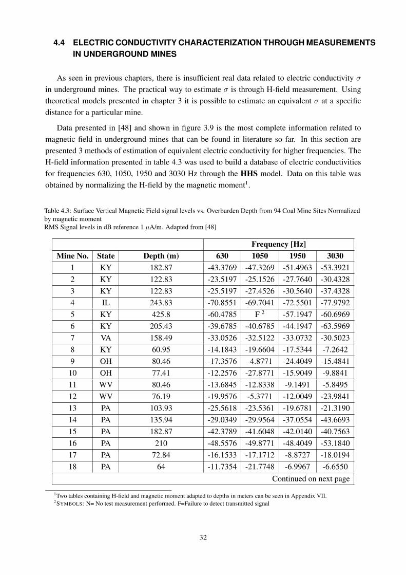
4.4 ELECTRIC CONDUCTIVITY CHARACTERIZATION THROUGH MEASUREMENTSIN UNDERGROUND MINES
As seen in previous chapters, there is insufficient real data related to electric conductivity σin underground mines. The practical way to estimate σ is through H-field measurement. Usingtheoretical models presented in chapter 3 it is possible to estimate an equivalent σ at a specificdistance for a particular mine.
Data presented in [48] and shown in figure 3.9 is the most complete information related tomagnetic field in underground mines that can be found in literature so far. In this section arepresented 3 methods of estimation of equivalent electric conductivity for higher frequencies. TheH-field information presented in table 4.3 was used to build a database of electric conductivitiesfor frequencies 630, 1050, 1950 and 3030 Hz through the HHS model. Data on this table wasobtained by normalizing the H-field by the magnetic moment1.
Table 4.3: Surface Vertical Magnetic Field signal levels vs. Overburden Depth from 94 Coal Mine Sites Normalizedby magnetic momentRMS Signal levels in dB reference 1 µA/m. Adapted from [48]
Frequency [Hz]Mine No. State Depth (m) 630 1050 1950 3030
1 KY 182.87 -43.3769 -47.3269 -51.4963 -53.39212 KY 122.83 -23.5197 -25.1526 -27.7640 -30.43283 KY 122.83 -25.5197 -27.4526 -30.5640 -37.43284 IL 243.83 -70.8551 -69.7041 -72.5501 -77.97925 KY 425.8 -60.4785 F 2 -57.1947 -60.69696 KY 205.43 -39.6785 -40.6785 -44.1947 -63.59697 VA 158.49 -33.0526 -32.5122 -33.0732 -30.50238 KY 60.95 -14.1843 -19.6604 -17.5344 -7.26429 OH 80.46 -17.3576 -4.8771 -24.4049 -15.484110 OH 77.41 -12.2576 -27.8771 -15.9049 -9.884111 WV 80.46 -13.6845 -12.8338 -9.1491 -5.849512 WV 76.19 -19.9576 -5.3771 -12.0049 -23.984113 PA 103.93 -25.5618 -23.5361 -19.6781 -21.319014 PA 135.94 -29.0349 -29.9564 -37.0554 -43.669315 PA 182.87 -42.3789 -41.6048 -42.0140 -40.756316 PA 210 -48.5576 -49.8771 -48.4049 -53.184017 PA 72.84 -16.1533 -17.1712 -8.8727 -18.019418 PA 64 -11.7354 -21.7748 -6.9967 -6.6550
Continued on next page
1Two tables containing H-field and magnetic moment adapted to depths in meters can be seen in Appendix VII.2SYMBOLS: N= No test measurement performed. F=Failure to detect transmitted signal
32

Table 4.3 – continued from previous pageFrequency[Hz]
Mine No. State Depth (m) 630 1050 1950 303019 PA 106.07 -29.3609 -28.6039 -29.0049 -29.750420 PA 103.93 -26.3859 -24.3789 -25.5485 -24.191821 PA 99.05 -27.6048 -31.0005 -35.6085 -44.425822 WV 173.43 -30.2809 -30.3155 -31.3303 -29.106123 VA 365.75 -70.8474 -71.8374 -70.8415 -67.836224 KY 82.29 -15.7914 -20.7155 -13.5783 -11.604225 VA 129.84 -28.5255 -28.3883 -35.4317 -33.519426 VA 210 -42.6053 -42.5727 -41.7208 -43.340027 VA 210 -39.1464 -40.3603 -40.2306 -38.743828 VA 157.88 -50.8408 -43.4443 -49.7550 -46.759729 VA 177.08 -36.7458 -37.0692 -35.6618 -34.600130 KY 99.05 -26.5618 -26.5361 -23.6780 -19.319031 VA 188.97 -39.9843 -39.6604 -39.5344 -36.064232 WV 100.88 -28.7405 -27.7903 -31.0101 -20.663933 WV 70.1 -16.9843 1.3655 -0.4382 -9.668434 WV 409.04 -68.2138 -71.6711 -79.3603 -79.833835 WV 99.05 -19.4377 -18.3155 -19.3645 -17.467236 WV 65.83 -9.3454 -11.2229 -12.2716 -3.869137 PA 145.99 -30.1913 -28.9766 -30.9514 -32.515538 WV 238.04 -44.9113 -47.2915 -54.9302 -67.877739 WV 154.83 -32.5618 -33.5361 -37.6780 -39.319040 AL 142.95 -22.8199 -25.7903 -28.8326 -30.772741 AL 147.82 -37.0576 -35.3771 -37.9049 -36.684142 AL 109.11 -23.2231 -20.5473 -22.0835 -20.883043 AL 89.91 -12.8197 -12.2526 -14.3640 -19.232844 AL 79.85 -11.1425 -17.3963 -16.3569 -9.603945 TN 288.03 -46.0418 -50.8775 -45.8897 -58.464946 TN 363.01 -55.0075 -58.0461 -58.4685 -68.931947 KY 79.85 -13.1100 -12.6959 -16.0727 -15.497648 KY 307.84 -49.4048 -52.1720 -52.1371 -52.689549 KY 145.99 -28.8322 -28.0589 -26.9967 -26.731150 IL 227.07 -58.2721 -67.1464 -56.2046 -68.809651 IL 85.03 -31.1224 -25.1774 -16.2556 -19.096852 IL 139.9 -29.6697 -31.9760 -33.4604 -36.237653 IL 197.81 -43.6139 -51.3562 -47.2783 -58.5393
Continued on next page
33

Table 4.3 – continued from previous pageFrequency[Hz]
Mine No. State Depth (m) 630 1050 1950 303054 IL 93.87 -19.3322 -40.5704 -27.9967 -27.731155 IL 88.08 -19.1913 -20.8766 -22.9514 -19.515556 WV 128.93 -23.6393 -23.9019 -24.3677 -23.130157 WV 320.03 -44.9966 -46.6765 -49.5473 -50.083558 WV 177.08 -33.2398 -34.2338 -35.3866 -36.028959 WV 117.95 -28.5576 -26.8771 -30.4049 -29.184060 WV 106.98 -20.2144 -20.2396 -17.6478 -16.340561 WV 257.86 N N N N62 WV 209.09 -53.4255 -53.6162 -53.9967 -56.731163 WV 147.82 -30.8436 -32.8698 -39.0716 -33.731764 WV 107.89 -26.4650 -24.5474 -23.8072 -20.480665 WV 71.01 -15.4255 -9.6162 -13.9967 -10.731166 WV 78.02 -43.4255 -25.6162 -8.9967 -34.731167 WV 128.01 -25.1612 -24.9454 -25.9143 -24.478868 WV 136.85 -40.3576 -39.2771 -41.3049 -42.284069 WV 131.06 F F -23.6923 -27.297970 WV 278.89 F F -63.0129 F71 PA 72.84 -7.1457 -5.9878 -11.0101 -12.595672 PA 146.91 -32.9682 -33.2187 -35.6609 -34.396573 PA 190.8 F -37.6767 -37.6696 F74 PA 145.99 -34.4377 -35.3155 F -37.967275 PA 200.55 -36.3522 -46.0922 -45.0251 -50.588576 UT 364.84 -57.8651 -56.2656 -68.4362 -75.177677 UT 304.79 -60.6271 -60.0182 -64.2923 -66.097978 UT 365.75 -53.2223 -56.6767 F -60.847879 CO 427.02 -64.1550 -71.3323 F F80 OH 152.39 -34.6576 -47.8771 -46.4049 -57.184081 OH 182.87 -39.9326 -42.6429 -48.6805 -58.712182 OH 142.95 -51.6363 -49.8307 -53.2023 -59.930883 OH 164.89 -43.2231 -44.5473 -47.0835 -52.883084 OH 170.99 -46.6815 -37.8641 -42.2361 -45.955485 KY 79.24 -15.7245 -14.8003 -13.0409 -11.709286 KY 152.09 -36.4377 -36.3155 -38.3645 -38.967287 KY 121.91 -30.7245 -30.8003 -31.0409 -27.709288 KY 115.82 -25.5018 -25.1983 -24.1840 -24.1967
Continued on next page
34

Table 4.3 – continued from previous pageFrequency[Hz]
Mine No. State Depth (m) 630 1050 1950 303089 AL 197.81 -37.1425 -37.3963 -37.8569 -40.603990 AL 472.74 -68.2223 -72.6767 -71.3696 -71.847891 KY 57.91 -13.3257 -2.7350 -8.3609 -16.187892 KY 79.85 -14.9377 -24.3155 -23.3645 -14.967293 KY 21.03 11.2888 12.8932 -23.7903 16.731494 KY 99.97 -25.5061 -29.7144 -37.9102 -45.2139
4.4.1 Equivalent electric conductivity over all frequencies and depths
Based on the magnetic field from Table 4.3 for every frequency and depths, it was estimatedthe equivalent electric conductivity using the HHS model. Figure 4.12 shows all σ estimated overall frequencies and depths:
0 50 100 150 200 250 300 350 40010−3
10−2
10−1
100
101 Conductivities over all frequencies and depths
Measurement index
Equi
vale
nt s
igm
a S/
m
Figure 4.12: Conductivities over all frequencies and depths
From this data, it is possible to identify the statistical distribution for σe. Through a compar-ison between Random Mean Square Errors (RMSE) for several distributions, it was generated aclassification Table 4.4 for deciding which distribution fits the best the data. For this method,it was identified the Log-normal distribution with parameters µ= -2.87014 dB and σ= 1.27042dB. Such parameters are fairly similar to those calculated in Section 4.3, which can sustain the
35

validity of this method.
Table 4.4: RMSE error over all frequencies and distances
Distribution RMSELog-normal 0.0060106Burr 0.0086287Loglogistic 0.010472GeneralizedExtremeValue 0.014665Weibull 0.019625Gamma 0.026832
4.4.2 Equivalent electric conductivity estimation as a function of frequency
Considering all distances in which H-field was measured, it was estimated the conductivityfor each frequency as seen in Figures 4.13 to 4.16. Again it was used the RMSE for creatingTable 4.5. From these result, it is possible to infer that conductivity reduces when frequencyrises. Such behavior may be associated to different field conditions (quasi-static, transition, far-field, etc.) suffered by fields with different frequencies in which simple models, such as HHScannot respond.
0 10 20 30 40 50 60 70 80 90 10010
−3
10−2
10−1
100
101
Mine index
Equiv
ale
nt sig
ma S
/m
Conductivities over all depths (for each frequency)
630 Hz
Figure 4.13: Conductivities over all depths 630 Hz
36

0 10 20 30 40 50 60 70 80 90 10010
−3
10−2
10−1
100
101
Mine index
Equiv
ale
nt sig
ma S
/m
Conductivities over all depths (for each frequency)
1050 Hz
Figure 4.14: Conductivities over all depths 1050 Hz
0 10 20 30 40 50 60 70 80 90 10010
−3
10−2
10−1
100
Mine index
Equiv
ale
nt sig
ma S
/m
Conductivities over all depths (for each frequency)
1950 Hz
Figure 4.15: Conductivities over all depths 1950 Hz
37

0 10 20 30 40 50 60 70 80 90 10010
−3
10−2
10−1
100
101
Mine index
Equiv
ale
nt sig
ma S
/m
Conductivities over all depths (for each frequency)
3030 Hz
Figure 4.16: Conductivities over all depths 3030 Hz
Table 4.5: RMSE error of conductivity distribution over all depths for each frequency
Distribution 630 Hz 1050 Hz 1950 Hz 3030 HzLog-normal 0.015891 0.010706 0.013781 0.015545Burr 0.011917 0.011181 0.010981 0.011891Gamma 0.022089 0.02612 0.02733 0.035226GeneralizedExtremeValue 0.022256 0.017913 0.013599 0.013227Loglogistic 0.018732 0.012352 0.014193 0.011777Weibull 0.01827 0.021948 0.022922 0.028261
From Table 4.5, it is observed that Log-normal distribution reaches a suitable fitting, andconsidering its symmetry in dB and simplicity, it is chosen for data normalization through its pa-rameter µ. Results for that normalization are shown in Figure 4.17. The characteristic parametersfor Log-normal distribution are µ=0 dB σ= 1.1701 dB. Comparing both results it is possible torealize that conductivities keep the same behavior. A remarkable difference that can be observedis that variation of equivalent σ is reduced after normalization in frequency.
38

0 10 20 30 40 50 60 70 80 90 10010−2
10−1
100
101
102
Mine index
Equi
vale
nt s
igm
a S/
m
Conductivities over all depths (normalized in frequency)
630 Hz1050 Hz1950 Hz3030 Hz
Figure 4.17: Conductivities over all depths (normalized in frequency)
4.4.2.1 Extrapolation of Log-normal parameters for frequencies beyond 3030 Hz
An estimation of parameters µ and σ of Log-normal distribution that describes equivalentconductivity is presented in Table 4.6 and in Figure 4.18. Such estimation was carried out by themeans of cubic spline interpolation and, subsequently, extrapolation with a 3rd order polynomial.
Table 4.6: Log-normal Distribution parameters of conductivity: over all depths (for each frequency) and extrapolatedMu values from 4350Hz to 10kHz
Frequency µ [dB] σ [dB]630 -2.1911 1.17711050 -2.6202 1.10571950 -3.1759 1.21203030 -3.4768 1.20414350 -3.807 -5970 -4.1922 -7850 -4.6392 -10000 -5.1503 -
39

0 1000 2000 3000 4000 5000 6000 7000 8000 9000 10000−5.5
−5
−4.5
−4
−3.5
−3
−2.5
−2
−1.5
frequency [Hz]
Mu
[dB]
Mu parameter: polynomial 3rd order extrapolation
estimatedextrapolated
Figure 4.18: µ parameter of Log-normal distribution for conductivity: polynomial 3rd order extrapolation
4.4.3 Equivalent electric conductivity estimation as a function of mine depth
It is important to estimate the variation of conductivity as a function of mine depth. Again,using data from Section 4.4.1, it was estimated a curve for equivalent conductivities Figure 4.19.
0 50 100 150 200 250 300 350 400 450 50010−3
10−2
10−1
100
101
Depth [m]
Equi
vale
nt s
igm
a S/
m
Conductivities for each frequency as a function of depth
630 Hz1050 Hz1950 Hz3030 Hz
Figure 4.19: Conductivities for each frequency as a function of depth
40

Due to depth distribution in the database, there were calculated different statistical distribu-tions for three groups of depths. The classification of fitting distributions can be found in tables 4.7to 4.9 and parameters for fitting distributions are presented in Tables 4.10 and 4.11 According tothis results, equivalent conductivity decreases as depth increases. This fact is usually relatedto higher conductivities inherent in surface or lower depths due to metal equipment/cables andsoil salinization. However, simulation results in Section 4.5 will show that the dependence ofequivalent conductivity on depth is also true even when there is not any upper layer with higherconductivity. In multi-layer conditions, the transitions through various layers appear to causemore attenuation to the field when it is in quasi-static or transition zone, leading to a pessimisticestimation of apparent conductivity for measurements at lower depths.
Table 4.7: RMSE error of conductivity distribution for each frequency for depths between 0 and 100 meters
Distribution 630 Hz 1050 Hz 1950 Hz 3030 HzLog-normal 0.026581 0.03822 0.036472 0.03152Burr 0.033005 0.029182 0.03752 0.030142Gamma 0.039023 0.040892 0.041438 0.051767Loglogistic 0.029427 0.02913 0.038843 0.032266Weibull 0.043136 0.042323 0.040548 0.043012
Table 4.8: RMSE error of conductivity distribution for each frequency for depths between 100 and 200 meters
Distribution 630 Hz 1050 Hz 1950 Hz 3030 HzLog-normal 0.024253 0.023005 0.043881 0.035353Burr 0.028294 0.02049 0.023493 0.023014Gamma 0.038121 0.025111 0.024466 0.023405Loglogistic 0.028137 0.021599 0.041669 0.034128Weibull 0.039953 0.029537 0.023432 0.024249
Table 4.9: RMSE error of conductivity distribution for each frequency for depths between 200 and 500 meters
Distribution 630 Hz 1050 Hz 1950 Hz 3030 HzLog-normal 0.044205 0.0483 0.052546 0.047364Burr Inf Inf 0.035293 InfGamma 0.063591 0.068918 0.036083 0.054153Loglogistic 0.04792 0.050442 0.051208 0.049498Weibull 0.056534 0.065842 0.035107 0.05294
Table 4.10: µ parameter in dB for Log-normal distribution of conductivity
Frequency [Hz] D: 0 to 100 m D: 100 to 200 m D: 200 to 500 m630 -1.12 -2.2042 -3.39671050 -1.7223 -2.7709 -3.46831950 -2.1317 -3.2491 -4.17333030 -2.699 -3.5825 -4.1933
41

Table 4.11: σ parameter in dB for Log-normal distribution of conductivity
Frequency [Hz] D: 0 to 100 m D: 100 to 200 m D: 200 to 500 m630 0.77296 0.80186 1.02421050 1.0706 0.83934 0.841341950 0.92617 0.96328 1.04283030 1.2674 0.97317 1.069
An estimation of equivalent conductivity normalized as in frequency as in depth is shown inFigure 4.20. The statistical distribution obtained is Log-normal with parameters µ = 0 dB, σ =0.94462 dB.
Finally, it was used the extrapolation method explained in the previous section for estimatingµ parameter of equivalent conductivity distribution for some frequencies from 630 Hz to 10 kHz.From this data, it is possible to realize that µ decreases as a function of distance and frequency.
Table 4.12: µ parameter in dB for Log Normal Distribution (for each frequency and depth interval)
Frequency [Hz] D: 0 to 100 m D: 100 to 200 m D: 200 to 500 m630 -1.12 -2.2042 -3.39671050 -1.7223 -2.7709 -3.46831950 -2.1317 -3.2491 -4.17333030 -2.699 -3.5825 -4.19334350 -3.3459 -3.9373 -4.21115970 -4.1388 -4.3567 -4.19497850 -5.0589 -4.8434 -4.176210000 -6.1111 -5.4 -4.1548
4.5 MULTI-LAYER STATISTICAL MODEL THROUGH ELECTROMAGNETIC FIELDSIMULATIONS
With the estimations calculated in section 4.4, specially in Table 4.6 for the middle frequency,a simulation set was created in order to study H-field behavior in close-to-reality scenarios. Thescenario used for that simulation is described as follows and it is shown in Figure 4.21:
• Antennae size: both antennae have a square shape with√π m side and square cross-
section of 1 cm2.
• Antennae position: the above ground antenna was set to be 50 cm over ground andin vacuum conditions. The second antenna was positioned at 300 m under surface of mine,inserted in the soil layer.
• Layer size: all layers are 50 m side square shaped parallelepipeds with different heights,which depends on the number of layers and the height overall layers is 310 m,
42
• Number of layers: a random number of layers X is selected from a uniform distribu-tion U(3, 25),
• Heights of layers: a random height is chosen from a uniform distributionU(1, 300/x)
where x is the number of layers sorted before,
• Probe position: probes for measuring H-field distributed evenly at the antennae axesat a 10 m distance of each other and at center of each antenna,
• Layer electromagnetic characteristics: magnetic permeability was set asvacuum condition µ0 = 4π10−7; electric conductivity was programmed to be a point of arandom Log-Normal distribution according to the extrapolated parameters from Table 4.6for frequency of 4350 Hz,
• Frequency range: 0.1 to 10 kHz distributed in logarithmic steps,
• Number of trials: 150 independent and random trials.
4.5.1 H-field variation as a function of depth and frequency
In order to have a general idea about the variation of H-field as a function of depth and fre-quency, it is interesting to see such variation for a single trial. Figure 4.22 shows that H-fielddecreases as depth and frequency augment.
Also, it is interesting to compare the simulated H-field to theoretical models of TS and HHS.In Figure 4.23 is shown the H-field for all frequencies and all trials, and TS and HHS overlappingthem. Is possible to infer that both theoretical models cannot suit the simulated field for anyconfiguration because H-field has a different behavior that is not predicted for them. Even ifsome conductive values are used to fit the H-field curve to the median of synthetic data for somefrequencies those will not be valid for other frequencies or depths.
Furthermore, is important to give a closer view to H-field variations. Thus, there were selectedthree frequencies close to those from the extrapolated data (657.9, 4328.8 and 10000 Hz) andthree depths (20, 150 and 300 m) from all available data. From now on, all fields are capturedfrom synthetic or measured data are normalized to the magnetic moment of their transmitters toimprove the comparisons M = I ×N × Stx = 0.28× 1× π.
Field variation as a function of depth is shown in Figure 4.24. From it, it is possible to infer:
• For short depths, the H-field is affected homogeneously for all frequencies,
• For mid depths, the frequency starts to influence more significantly the attenuation of H-field and also it starts to augment its variation from mine to mine,
• For long depths, both H-field attenuation and variation are hoisted in higher intensity. Suchstronger field dependence on frequency for deeper depths is natural and also is noticed inIC, HHS and TS models.
43

Now, regarding to H-field variation as a function of depth, Figure 4.25, shows this variationfor three frequencies. It is possible to see that attenuation augments non-linearly with depth forall frequencies. Also, variation of H-field is more severe for deeper positions for all frequencies.
For each pair of frequency/depth there is a statistical distribution that fits the best the data. Allfields are taken in dB to fit distributions due to the importance of fields on very low levels. Again,it was used the RMSE as decision parameter. The tables 4.14 and 4.13 show the distribution foundand the RMSE for each combination. From the first one, it is possible to identify Burr as the mostfrequent distribution.
Table 4.13: H-field distribution for each pair of depth/frequency
Frequency Depth20 m 150 m 300 m
657.9 Hz Burr Extreme Value Generalized Extreme Value4328.8 Hz Burr Weibull Lognormal10 kHz Burr Burr Lognormal
Table 4.14: RMSE of field distribution for each pair of depth/frequency
Frequency Depth20 m 150 m 300 m
657.9 Hz 0.0162 0.0147 0.01174328.8 Hz 0.0156 0.0162 0.012810 kHz 0.0158 0.0120 0.0109
Regarding mean and standard deviation, tables 4.15 and 4.16 resume those statistical param-eters found. All related figures can be found in Appendix VIII.
Table 4.15: Mean value for H-field for three depths and three frequencies
Frequency Depth20 m 150 m 300 m
657.9 Hz -102.0837 -152.7302 -178.42324328.8 Hz -102.5094 -166.3229 -210.290510 kHz -103.2016 -179.2336 -235.5912
Table 4.16: Standard deviation for H-field for three depths and three frequencies
Frequency Depth20 m 150 m 300 m
657.9 Hz 4.2795 3.2247 5.21734328.8 Hz 4.5272 8.5019 12.919610 kHz 4.9979 11.1981 17.2684
44

4.5.2 H-field median fitting
In order to describe H-field in a more general way, it was calculated the median of all trialsas function of frequency and depth. Then, it was estimated the following empirical equation forH-field as a function of frequency and depth. Figure 4.26 shows the median values of H-field foreach pair of frequency (f ) and depth (d)and the fitting plane of the equation in (4.1)
H50(d, f) =20[a1 + a2 × log(ω) + a3 × log(d) + a4 × log(e−T )] [dB] (4.1)
For ω = 2πf and T = d√
ωµσ02
. σ0 = 0.025 is the equivalent value of mean conductivity usedin all simulations. This formula has R-square: 1.0000 and RMSE: 0.1506. The other coefficientsare presented in Table 4.17
Table 4.17: H-field median coefficients
Coefficient Valuea1 -2.821a2 0.233a3 -2.335a4 1.053
It is important to remember that this equation fits the median of H-field data extracted frommulti-layer simulations with conductivity following Log-normal distribution with parameters µ =
3.807 and σ = 1.196. These values are extrapolated from measured field data. Other less complexequations of lower order are easily computed bringing simplicity for the model at the cost ofincreasing the RMSE.
45

50
100
150
200
250
300
2000
4000
6000
8000
10000
−280
−260
−240
−220
−200
−180
−160
−140
−120
−100
Frequency Hz
Fitting curve for Normalized H−field median
Depth m
No
rma
lize
d H
−fie
ld
Surface Fitting H50
H50
(a) 3D H-field median fitting
50 100 150 200 250 300−280
−260
−240
−220
−200
−180
−160
−140
−120
−100
Depth m
Fitting curve for Normalized H−field median
No
rma
lize
d H
−fie
ld
Surface Fitting H50
H50
(b) 2D H-field median fitting
Figure 4.26: H-field median fitting
Figure 4.27 shows a comparison between H-field median calculated from simulations (sur-face) and measured data field from Table 4.3 only for the four frequencies employed in measure-ments. It is possible to infer that all simulations have resemblance to real data up to 250 m. Takinginto account that data from simulations was taken from 20 to 300 m, it is possible to suggest thatthe model simulated is valid, including the choice of layer and conductivity distributions and theirparameters.
46

50100
150200
250300 0
1000
2000
3000
4000−220
−200
−180
−160
−140
−120
−100
Frequency Hz
Depth
Norm
aliz
ed H
−field
(a) 3D view H-field median vs real data
50 100 150 200 250 300−220
−200
−180
−160
−140
−120
−100
Depth
No
rma
lize
d H
−fie
ld
(b) 2D view H-field median vs real data
Figure 4.27: H-field median compared to real condition data
4.5.3 Equivalent conductivity
It was calculated the median of equivalent conductivity for all trials by the means of HHSmodel and compared to equivalent conductivities computed from measured data mentioned ear-lier only the frequencies 630, 1050, 1950 and 3030 Hz. From the images in Figure 4.28, it ispossible to infer that simulated scenarios suit real conditions at least up to 300 m depth. Also, it is
47

possible to infer that the affirmation stated by Lincan in [31] "In the thin sheet model... the highlyconducting thin sheet represents possible surface metal structures, such as cables, pipes, casedbore hole, etc., as well as the relatively high conductivity at surface which usually contains moredissolved salt and mineral substances." is possibly mistaken by the observation of high equivalentconductivities in upper overburden when calculated through HHS and Q-factor models. This isdemonstrated by the simulations carried out in this dissertation, that even not employing any highconductive layer close the surface, still there are higher equivalent conductivities for small depthsas it can be seen in Figure 4.28.
48

50
100
150
200
250
300500
10001500
20002500
30003500
4000
10−3
10−2
10−1
100
101
Frequency [Hz]Depth [m]
Equiv
ale
nt sig
ma [S
/m]
(a) 3D view conductivity median vs real data
50 100 150 200 250 30010
−3
10−2
10−1
100
101
Depth [m]
Equiv
ale
nt sig
ma [S
/m]
(b) 2D view conductivity median vs real data
Figure 4.28: Median of Equivalent Conductivity compared to real condition data
49

4.6 ISSUES SOLVED WHILE USING THE COMMERCIAL SIMULATOR
Several situations where presented while simulation TTE environments. The most remarkableare:
• The use of higher conductivities (higher than 2 S/m) in the first conductive layer for down-link introduces numerical errors in magnetic field calculations. This happens due to inaccu-racies in modeling the boundary conditions for a diffusion medium.
• A small proportion between antenna size and the simulation boundary box size also intro-duces errors on calculation of magnetic field.
• Mesh size of 3D objects must be smaller for more conductive elements.
• The simulation time is reduced while using less layers while using the multi-layer model.
50

0 1000 2000 3000 4000 5000 6000 7000 8000 9000 10000−60
−50
−40
−30
−20
−10
0
Frequency Hz
Norm
aliz
ed fie
ld to q
uasi−
sta
tic [dB
]
IC
HHS
TS
σd=100
(a) H-field for σd=100
0 1000 2000 3000 4000 5000 6000 7000 8000 9000 10000−60
−50
−40
−30
−20
−10
0
Frequency Hz
Norm
aliz
ed fie
ld to q
uasi−
sta
tic [dB
]
IC
HHS
TS
σd = 20
(b) H-field for σd=20
Figure 4.3: H-field TS and HHS models variation of parameters σd
51

300 m
40 m
Conductive Homogeneous
Medium h
Figure 4.4: Simulation scenario for HHS model simulation
52

0 5 10 15 20 25 30 35 40 45 50
10−4.5
10−4.4
10−4.3
10−4.2
H−field for fix number of layers, Position= 50 m
Number of mine
Magnetic
field
[T
]
(a) H-field distribution
2 3 4 5 6 7 8
x 10−5
0
2
4
6
8
10
12x 10
4
Data
Pro
babili
ty d
istr
ibution
H−field PDF Distribution fitting, Position= 50 m
Data
ExtremeValue
Weibull
Normal
(b) Statistical fitting
Figure 4.6: H-field statistical characterization at 50 mFix number of layers
53

0 5 10 15 20 25 30 35 40 45 5010
−8
10−7
10−6
10−5
H−field for fix number of layers, Position= 110 m
Number of mine
Ma
gn
etic f
ield
[T
]
(a) H-field distribution
0 1 2 3 4 5 6 7
x 10−6
0
1
2
3
4
5
6
7x 10
5
Data
Pro
ba
bili
ty d
istr
ibu
tio
n
H−field PDF Distribution fitting, Position= 110 m
Data
Normal
GeneralizedPareto
Rayleigh
(b) Statistical fitting
Figure 4.7: H-field statistical characterization at 110 mFix number of layers
54

0 5 10 15 20 25 30 35 40 45 5010
−9
10−8
10−7
10−6
10−5
H−field for fix number of layers, Position= 150 m
Number of mine
Ma
gn
etic f
ield
[T
]
(a) H-field distribution
0 0.2 0.4 0.6 0.8 1 1.2
x 10−6
0
0.5
1
1.5
2
2.5
3
3.5
4
4.5x 10
6
Data
Pro
babili
ty d
istr
ibution
H−field PDF Distribution fitting, Position= 150 m
Data
GeneralizedPareto
Weibull
Exponential
(b) Statistical fitting
Figure 4.8: H-field statistical characterization at 150 mFix number of layers
55

0 5 10 15 20 25 30
104.5
104.4
104.3
104.2
H field for random number of layers, Position= 50 m
Number of mine
Magnetic
eld
[T]
(a) H-field distribution
2 3 4 5 6 7 8
x 10−5
0
1
2
3
4
5
6
7
8x 10
4
Data
Pro
ba
bili
ty d
istr
ibu
tio
n
H−field PDF Distribution fitting, Position= 50 m
Data
ExtremeValue
tLocationScale
Logistic
(b) Statistical fitting
Figure 4.9: H-field statistical characterization at 50 mRandom number of layers
56

0 5 10 15 20 25 3010
−7
10−6
10−5
H−field for random number of layers, Position= 110 m
Number of mine
Magn
etic fi
eld
[T
]
(a) H-field distribution
0 1 2 3 4 5 6 7 8
x 10−6
0
1
2
3
4
5
6
7x 10
5
Data
Pro
ba
bili
ty d
istr
ibu
tio
n
H−field PDF Distribution fitting, Position= 110 m
Data
Loglogistic
Burr
GeneralizedExtremeValue
(b) Statistical fitting
Figure 4.10: H-field statistical characterization at 110 mRandom number of layers
57

0 5 10 15 20 25 3010
−8
10−7
10−6
10−5
H−field for random number of layers, Position= 150 m
Number of mine
Ma
gn
etic fi
eld
[T
]
(a) H-field distribution
0 0.2 0.4 0.6 0.8 1 1.2 1.4 1.6 1.8
x 10−6
0
0.5
1
1.5
2
2.5
3
3.5
4x 10
6
Data
Pro
babili
ty d
istr
ibution
H−field PDF Distribution fitting, Position= 150 m
Data
Burr
Loglogistic
GeneralizedExtremeValue
(b) Statistical fitting
Figure 4.11: H-field statistical characterization at 110 mRandom number of layers
58

0 50 100 150 200 250 300 350 400 450 50010−2
10−1
100
101
102
Depth [m]
Equi
vale
nt s
igm
a S/
m
Conductivities (normalized in frequency and depth)
630 Hz1050 Hz1950 Hz3030 Hz
Figure 4.20: Conductivities (normalized in frequency and depth)
300 m
50 m
Conductive
Medium σi
Figure 4.21: Multi-layer TTE scenario
59

0
50
100
150
200
250
300
0
2
4
6
8
10Depth m
Frequency [kHz]
H−
field
dB
−250
−200
−150
−100
Figure 4.22: H-field variation for a single mine as a function of depth and frequency
Frequency kHz
H−
field
dB
0 1 2 3 4 5 6 7 8 9 10−280
−260
−240
−220
−200
−180
−160
−140
HHS
TS
Figure 4.23: H-field variation for a single mine as a function of depth and frequency
60

10−1
100
101
−350
−300
−250
−200
−150
−100
−50
Frequency kHz
Norm
aliz
ed H
−field
dB
Normalized magnetic field for 3 depths and all frequencies
20 m
150 m
300 m
Figure 4.24: H-field variation as a function of depth for 3 positions.
0 50 100 150 200 250 300−350
−300
−250
−200
−150
−100
−50
Depth m
Norm
aliz
ed H
−field
dB
Normalized magnetic field for 3 frequencies and all depths
657.9 Hz
4328.8 Hz
10000 Hz
Figure 4.25: H-field variation as a function of frequency.
61

5 CONCLUSION
An alternative to wire based systems in underground mines is the Through-The-Earth com-munication system, specially in situations where human beings are trapped underground due totunnel burials that brakes wired links to surface. Other application for the TTE systems is theactivation of explosives and automation of equipment for underground mining.
Wireless propagation, especially Through-The-Earth, establishes severe restrictions to thecommunication system. Using low-frequency signals is essential for reducing the effects of soilattenuation in underground environments. Soil electric characteristics potentiate such attenua-tion, so having the same information about the environment makes easier the process of planningcommunication structure for a underground mines.
As it has been shown in this dissertation, theoretical models TS and HHS does not describedproperly magnetic field propagation with a variety of media, and other models are too complex toimplement that makes almost impossible to used them.
Magnetic field is affected in both depth and frequency dimensions in stratified TTE commu-nication environments. H-field is affected in less proportion for small distances, where frequency(from 0.1 to 10 kHz) does not affect significantly the communication link. For further depths, fre-quency introduces more variation of H-field for different mine sites, as well as bigger attenuationof signal as it can be seen in Tables 4.15 and 4.16.
Regarding equivalent conductivity, according to TS model, equivalent conductivity is higherfor smaller depths due to the presence of highly conductive elements. Nevertheless, according tothe simulations presented in the previous chapter, for scenarios where no TS was contemplated,the equivalent conductivity kept higher values for small depths.
As presented in previous chapters, soil electric conductivity can be an important parameterto be taken into account while transmitting signals through the earth. For an arbitrary mine con-figuration, after estimating the distance between both endpoints and frequency, it is possible touse the empirical equation of H-field presented in this dissertation for predicting the median ofreceived magnetic field for mines with similar soil characteristics as coal mines. With this infor-mation, it is possible to adequate all parameters from the transmitter and receiver for an efficientcommunication.
TTE communication is a field that has not been extensively studied, therefor there are severaltopics that can be researched after the present work. Among those topics are the following:
• Propagation channel modeling: as it was seen, TS and HHS models do not predict magneticfield attenuation and other models are difficult to implement. Because of that, there isa necessity of more accurate and practical models for magnetic field propagating in TTEenvironments.
62

• Antennae, transmission/reception circuits and impedance matching circuits: it is necessaryto improve the research on high sensibility antennae or magnetic sensor inside conductivemedium and all circuits related to them.
• Localization techniques based on multi-sensor networks: this application is vital for sensingmine status prior disasters and after any emergency situation where miners are trapped.
• Studies of field behavior in multi-layer media in quasi-static, near-field, transition and far-field zones to better understand the effect of high equivalent conductivities in upper layers.
63

BIBLIOGRAPHICAL REFERENCES
1 BARKAND, T. D.; DAMIANO, N. W.; SHUMAKER, W. Through-the-earth, two-way, mineemergency, voice communication systems. In: IEEE. Industry Applications Conference, 2006. 41st IASAnnual Meeting. Conference Record of the 2006 IEEE. [S.l.], 2006. v. 2, p. 955–958.
2 RAAB, F. H.; JOUGHIN, I. R. Signal processing for through-the-earth radio communication.Communications, IEEE Transactions on, IEEE, v. 43, n. 12, p. 2995–3003, 1995.
3 YENCHEK, M. R.; HOMCE, G. T.; DAMIANO, N. W.; SREDNICKI, J. R. Niosh-sponsored researchin through-the-earth communications for mines: a status report. Industry Applications, IEEE Transactionson, IEEE, v. 48, n. 5, p. 1700–1707, 2012.
4 MINERAL, D. N. de Produção. Código de Mineração - Capítulo I das Disposições Preliminares.Http://www.dnpm-pe.gov.br/Legisla/cm_01.htm. Accessed: 2015-04-22. Available at: <http://www.dnpm-pe.gov.br/Legisla/cm\_01.htm>.
5 YARKAN, S.; GÜZELGÖZ, S.; ARSLAN, H.; MURPHY, R. Underground mine communications: Asurvey. Communications Surveys Tutorials, IEEE, v. 11, n. 3, p. 125–142, rd 2009. ISSN 1553-877X.
6 (UNDERGROUND), A. M. T. MAGNETO MINE TELEPHONES. 2012.Http://www.britishtelephones.com/ atm/atmtel6.htm. Accessed: 2015-04-15. Available at:<http://www.britishtelephones.com/atm/atmtel6.htm>.
7 BANDYOPADHYAY, L.; CHAULYA, S.; MISHRA, P. Wireless communication in undergroundmines. RFID-Based Sens. Netw, Springer, 2010.
8 SAFETY, N. I. for O.; HEALTH. Tutorial on Wireless Communication and ElectronicTracking Part 1: Technology Overview. 2010. Http://www.msha.gov/techsupp/PEDLocating/WirelessCommandTrack2009.pdf. Accessed: 2015-04-22. Available at: <http://www.msha.gov/techsupp/PEDLocating/WirelessCommandTrack2009.pdf>.
9 PATRI, A.; NAYAK, A.; JAYANTHU, S. Wireless communication systems for underground mines–acritical appraisal. International Journal of Engineering Trends and Technology (IJETT), v. 4, n. 7, p.3149–3153, 2013.
10 YIN, Z. J.; CHUNG, K.-S. Multiple access protocol for an underground mobile communicationsystem. In: Global Telecommunications Conference, 1998. GLOBECOM 1998. The Bridge to GlobalIntegration. IEEE. [S.l.: s.n.], 1998. v. 4, p. 2217–22224.
11 JING, G.; QIANPING, W. Application of hybrid routing protocol for mine WSN. In: EnvironmentalScience and Information Application Technology (ESIAT), 2010 International Conference on. [S.l.: s.n.],2010. v. 3, p. 353–355.
12 CHETAN, B.; DESHPANDE, P.; HEGDE, B. G.; SRINIVAS, S.; KUMAR, G. N. Analysis of DSdvamp; aodv for disaster management system in coal mines. In: Wireless Communications, Networkingand Mobile Computing (WiCOM), 2011 7th International Conference on. [S.l.: s.n.], 2011. p. 1–4. ISSN2161-9646.
13 LEI, S.; ZHAO, X.; WENYAN, Z.; XICHENG, C. Model of ad hoc networks for rescuing in mine.In: Networks Security Wireless Communications and Trusted Computing (NSWCTC), 2010 SecondInternational Conference on. [S.l.: s.n.], 2010. v. 1, p. 210–213.
64

14 WU, D.; LI, R.; BAO, L. A holistic routing protocol design in underground wireless sensor networks.In: Mobile Ad-hoc and Sensor Networks, 2008. MSN 2008. The 4th International Conference on. [S.l.:s.n.], 2008. p. 187–194.
15 SUN, Y.; LIU, X. Wireless multi-hop ad hoc networks based on olsr for underground coal mine. In:Wireless Communications and Signal Processing (WCSP), 2010 International Conference on. [S.l.: s.n.],2010. p. 1–6.
16 WENQI, C.; ZHAO, X. Multi-hop routing for wireless network in underground mines. In: WearableComputing Systems (APWCS), 2010 Asia-Pacific Conference on. [S.l.: s.n.], 2010. p. 337–340.
17 JIANG, H.; PENG, J.; PENG, W. Nonuniform clustering routing protocol for tunnel wireless sensornetwork in underground mine. In: Wireless Communications Signal Processing, 2009. WCSP 2009.International Conference on. [S.l.: s.n.], 2009. p. 1–5.
18 ZHENG, Z.; HU, S. Research challenges involving cross-layered communication protocol designfor underground WSNs. In: Anti-counterfeiting, Security and Identification, 2008. ASID 2008. 2nd
International Conference on. [S.l.: s.n.], 2008. p. 120–123.
19 AL., G. S. et. To the rescue! 2010. World Coal.
20 NEWS, E. New Through Earth Communication System for Coal Mining. 2014. Endeavour Magazine.
21 FOROOSHANI, A.; BASHIR, S.; MICHELSON, D.; NOGHANIAN, S. A survey of wirelesscommunications and propagation modeling in underground mines. Communications Surveys Tutorials,IEEE, v. 15, n. 4, p. 1524–1545, Fourth 2013. ISSN 1553-877X.
22 GIBSON, D. Channel Characterisation and System Design for Sub-Surface Communications. Tese(Doutorado) — University of Leeds, Feb. 2003.
23 BALANIS, C. Antenna Theory: Analysis and Design. 3rd. ed. [S.l.]: John Wiley and Sons, 2005.
24 GRIFFITHS, D. J. Introduction to Electrodynamics. 3a. ed. [S.l.]: Prentice Hall, 1999.
25 STARKEY, D. B. Electromagnetic transmission and detection at deep depths. Sandia LaboratoriesReport SLL-73-5278, 1973.
26 WAIT, J. R. Electromagnetic induction technique for locating a buried source. Geoscience Electronics,IEEE Transactions on, v. 9, n. 2, p. 95–98, Apr. 1971. ISSN 0018-926X.
27 WAIT, J. R.; SPIES, K. Subsurface electromagnetic fields of a circular loop of current located aboveground. Antennas and Propagation, IEEE Transactions on, v. 20, n. 4, p. 520–522, July. 1972. ISSN0018-926X.
28 DURKIN, J. Surface vertical magnetic field produced by a finite loop buried in an earth containing athin conducting sheet. Radio Science, Wiley Online Library, v. 32, n. 1, p. 19–23, 1997.
29 ADMINISTRATION, O. S. . H. Electromagnetic Radiation: Field Memo. Accessed: 2015-02-22.Available at: <https://www.osha.gov/SLTC/radiofrequencyradiation/electromagnetic_fieldmemo/electromagnetic.html#section_6>.
30 DA, W. J. H. Theoretical noise and propagation models for through-the-earth communication. [S.l.],1982.
31 LINCAN, Y. Measurements and modeling of the electromagnetic fields in Through-The-Earth (TTE)wireless communications. Tese (Doutorado) — University of New Mexico, 2014.
65

32 L., H. H.; M., M. J. Introductory mining engineering. [S.l.]: John Wiley, 2002.
33 HEM, P.; CALDWELL, J. Block Caving. Accessed: 2015-01-04. Available at: <http://technology.infomine.com/reviews/Blockcaving/welcome.asp?view=full>.
34 PRESS, A. September U.S. Mine Inspections Result in 133 Citations. 2015. Accessed: 2015-11-5.Available at: <http://wvpublic.org/post/september-us-mine-inspections-result-133-citations>.
35 RATCLIFFE, M. Anglo American shares fall as miner completes sale of Norte copper mine aftercommodities fall hits profits. 2015. Accessed: 2015-10-01. Available at: <http://www.cityam.com/224250/anglo-american-completes-sale-of-norte-copper-mine-after-commodities-fall-hits-profits>.
36 ATM MINING TELEPHONES (UNDERGROUND). 2014. Accessed: 2014-09-30. Available at:<http://www.britishtelephones.com/atm/atmtel6.htm>.
37 AGGARWAL, R.; MOORE, P. Digital communications for protection. iii. fibre optics. PowerEngineering Journal, v. 8, n. 5, p. 241–246, Oct. 1994. ISSN 0950-3366.
38 ON-LINE, C. 95% of municipalities have fiber optics in 5 years. 2015. Ac-cessed: 2015-12-04. Available at: <http://www.confirmeonline.com.br/confirme/en/noticias/95-dos-municipios-terao-fibra-otica-em-5-anos>.
39 CONTROL, C. for D.; PREVENTION. Advanced Tutorial on Wireless Communication andElectronic Tracking: Communication System Performance. Accessed: 2014-05-12. Availableat: <http://www.cdc.gov/niosh/mining/content/emergencymanagementandresponse/commtracking/advcommtrackingtutorial2.html>.
40 EXCHANGE, P. S. Transverse Magnetic (TM) and Transverse Electric (TE) modes.Accessed: 2016-01-02. Available at: <http://physics.stackexchange.com/questions/78419/transverse-magnetic-tm-and-transverse-electric-te-modes>.
41 PEI, Z.; DENG, Z.; YANG, B.; CHENG, X. Application-oriented wireless sensor networkcommunication protocols and hardware platforms: A survey. In: Industrial Technology, 2008. ICIT 2008.IEEE International Conference on. [S.l.: s.n.], 2008. p. 1–6.
42 BANDYOPADHYAY, L. K.; CHAULYA, S. K.; MISHRA, P. K. Wireless Communication inUnderground Mines: RFID-based Sensor Networking. 1st. ed. [S.l.]: Springer Publishing Company,Incorporated, 2009. ISBN 0387981640, 9780387981642.
43 HUBING, T. H. Survey of Numerical Electromagnetic Modeling Techniques. [S.l.], 1991.
44 ZHANG, Q.; LI, W. Research on channel characteristics of through-the-earth communication basedon fdtd method. 2014 Sixth International Conference on Measuring Technology and MechatronicsAutomation, IEEE Computer Society, Los Alamitos, CA, USA, v. 3, p. 35–37, 2010.
45 L, A. N. C. J. A. M. A. L. F. V. J. Through-the-earth magnetic field propagation: Modelling forunderground applications,. Electromagnetics in Advanced Applications, 2009. ICEAA ’09. InternationalConference, p. 525 – 528, 2009.
46 SOUTERWEB. ASSEMBLY OF THE 2008 DQ RECEIVER BOARDS WITH THE NEW 3496Hz CLASS-E HIGH_EFFICIENCY BEACON DESIGN. 2008. Accessed: 2016-01-09. Available at:<http://souterweb.free.fr/boitaoutils/prospection/annexes/NotesOnThe2008_DQReceiverBoards.html>.
47 DURKIN, J. Apparent Earth Conductivity Over Coal Mines as Estimated From Through-The-EarthElectromagnetic Transmission Tests. 1984. Available at: <http://www.cdc.gov/niosh/mining/userfiles/works/pdfs/ri8869.pdf>.
66

48 LITTLE, I. A. Detection of trapped miner eLecetromagetic signals above coal mines. [S.l.], 1980.
49 MSHA. Mine Improvement and New Emergency Response Act of 2006. 2006. Accessed: 2016-01-06.Available at: <http://www.msha.gov/mineract/MineActAmmendmentSummary.asp>.
50 FRAGOSO, C. R. Root mean square error (RMSE). Available at: <http://www.ctec.ufal.br/professor/crfj/Graduacao/MSH/Model%20evaluation%20methods.doc.>
51 THE UNIVERSITY OF ALABAMA IN HUNTSVILLE. The Lognormal Distribution.The University of Alabama in Huntsville, Shelby Center for Science and Technology, Room258A, 301 Sparkman Drive, Huntsville, AL 35899, US. Access: 2016-01-30. Available at:<http://www.math.uah.edu/stat/special/LogNormal.html>.
67

APPENDIX
68

I. MINER ACT OF 2006
The following text was extracted from United States Department of Labor website in January6th 2016 [49]
"The Mine Improvement and New Emergency Response Act of 2006 would require operatorsof underground coal mines to improve accident preparedness. The legislation would require min-ing companies to develop an emergency response plan specific to each mine they operate, andrequire that every mine have at least two rescue teams located within one hour. S. 2803 wouldalso limit the legal liability of rescue team members and the companies that employ them. The actwould increase both civil and criminal penalties for violations of federal mining safety standardsand would give the Mine Safety and Health Administration (MSHA) the ability to temporarilyclose a mine that fails to pay the penalties or fines. In addition, the act calls for several studiesinto ways to enhance mine safety, as well as the establishment of a new office within the NationalInstitute for Occupational Safety and Health devoted to improving mine safety. Finally, the leg-islation would establish new scholarship and grant programs devoted to training individuals withrespect to mine safety.
Key Provisions of the MINER Act:
• Require each covered mine to develop and continuously update a written emergency re-sponse plan;
• Promote use of equipment and technology that is currently commercially available;
• Require each mine’s emergency response plan to be continuously reviewed, updated andre-certified by MSHA every six months;
• Direct the Secretary of Labor to require wireless two-way communications and an electronictracking system within three years, permitting those on the surface to locate persons trappedunderground;
• Require each mine to make available two experienced rescue teams capable of a one hourresponse time;
• Require mine operators to make notification of all incidents/accidents which pose a reason-able risk of death within 15 minutes, and sets a civil penalty of $5,000 to $60,000 for mineoperators who fail to do so;
• Establish a competitive grant program for new mine safety technology to be administeredby NIOSH;
• Establish an inter-agency working group to provide a formal means of sharing non-classifiedtechnology that would have applicability to mine safety;
69

• Raising the criminal penalty cap to $250,000 for first offenses and $500,000 for second of-fenses, as well as establishing a maximum civil penalty of $220,000 for flagrant violations;
• Give MSHA the power to request an injunction (shutting down a mine) in cases where themine has refused to pay a final order MSHA penalty;
• Create a scholarship program available to miners and those who wish to become minersand MSHA enforcement staff to head off an anticipated shortage in trained and experiencedminers and MSHA enforcement;
• Establish the Brookwood-Sago Mine Safety Grants program to provide training grants tobetter identify, avoid and prevent unsafe working conditions in and around the mines. Thesegrants will be made on an annual, competitive basis to provide education and training foremployers and miners, with a special emphasis on smaller mines."
70

II. 3D MAGNETIC FIELD SIMULATION ON CST STUDIOSUITE
The following pages present a brief manual on how to build a simulation scenario for a TTEtransmission system using the commercial software CST STUDIO SUITE.
For building the TTE transmission simulation computer environment, it is necessary to es-tablish simulator options and constructing the simulation scenario. CST comes with a nativeapplication within the application that permit customization and simulation settings in a easysequence as listed below:
1. Select an application area and a workflow. The application area depends on license pur-chased. For this investigation was acquired the Microwaves, Radio Frequencies and Opticallicense. This area opens six workflows: Antennas; Circuit & Components; Radar CrossSection; Biomedical, Exposure, SAR; Optical Applications, and Periodic Structures. Alsoit is possible to improve the workflow selection through more options according to eachitem.
2. Select the numerical method solver. According to each workflow, the software will suggestthose methods recommended.
3. Select simulation units. For every simulation it is necessary to determine which units willbe used for 3D structure building and simulation results.
4. Introduce frequency range or simulation time depending on selected method. In this stageis possible to determine frequency monitors for sensing E-field, H-Field, Power flow, Powerlosses and Far-field magnitudes.
5. 3D Structure construction. This stage is where physical characteristics of environment aredefined. Using several 3D CAD functions is feasible to construct all structures needed.There is a grand material library for choosing from and it is possible to create new materialsto fulfill specific conditions. Additionally, external CAD projects can be used to improvestructure building velocity.
Aiming an acceptable relation between processing time and accuracy, it is important to selecta suitable meshing of all structures and numerical method. CST offers two meshing options, atetrahedral and hexahedral. Such option controls simulation time and it is available for both timeand frequency domain. Figure II.1 shows how meshing adapts to each structure depending onits geometric characteristics. For simpler structures as cubic blocs, this adaptive meshing allowsusing bigger cells which diminish total node number and reduces time processing.
71

Figure II.1: Tetrahedral meshing
Border conditions are chosen in such way that numerical calculations can converge. Thatsoftware offers usual conditions as: electric or magnetic planes, free space, conductive walls,periodic characteristic walls and unit cells. In figure II.2, all open boundaries are selected.
Figure II.2: Border conditions
Field intensities can be measured using probes located on positions of interest. Among thatdata, it is possible to measure voltages, currents, S parameters, and Z and Y matrix through portson radiating structures. Generally, those responses are shown in 2D or 3D graphics, which canuse several representations as logarithmic, polar, phase and magnitude. Some of them can bevisualized as 3D animated images as a function of time and space changing colors for giving
72

motion sensation. Also, it is feasible to use 3D vector plots with arrows, cones, hedgehog shapelines and streamlines that moves according to field’s direction. In figure II.3 is represented aframe of an animated 3D image where is indicated magnetic field variations on space.
Figure II.3: Magnetic field inside substrates
Commercial software, as CST STUDIO SUITE, have post-processing tools that include pro-grammable routines. Result data can be processed directly at CST for generating new graphicsand comparing them to theoretical data without using any other software. Additionally, for somemore complex calculation it is possible to use VBA code for upgrading post-processing analysis.Next figure represents a result obtain with CST.
Figure II.4: Current result in linear scale
73

III. ROOT MEAN SQUARE ERROR (RMSE)
Fragoso in [50] described the RMSE as follows: "The Root Mean Square Error (RMSE) (alsocalled the root mean square deviation, RMSD) is a frequently used measure of the differencebetween values predicted by a model and the values actually observed from the environment thatis being modeled. These individual differences are also called residuals, and the RMSE serves toaggregate them into a single measure of predictive power.
The RMSE of a model prediction with respect to the estimated variable Xmodel is defined asthe square root of the mean squared error:
RMSE =
√∑ni=1 (Xobs,i −Xmodel,i)
2
n
where Xobs is observed values and Xmodel is modeled values at time/place i.
The calculated RMSE values will have units, and RMSE for phosphorus concentrations canfor this reason not be directly compared to RMSE values for chlorophyll a concentrations etc.However, the RMSE values can be used to distinguish model performance in a calibration periodwith that of a validation period as well as to compare the individual model performance to that ofother predictive models."
74

IV. LOGNORMAL DISTRIBUTION
A definition of the UAH in [51] states that: "A random variableX has a lognormal distributionwith parameters µ ∈ R and σ ∈ (0,∞) if ln(X) has the normal distribution with mean µ andstandard deviation σ. The parameter σ is the shape parameter of X and eµ is the scale parameterof X ."
In other words, X = eY and Y has normal distribution with mean µ and standard deviation σ.It is possible to rewrite the equation as a function of a normally distributed random variable Z toobtain: Y = µ + σZ. This distribution is used to model continuous random quantities when thedistribution is believed to be skewed.
The probability density function (PDF) with parameters µ and σ is described by:
f(x) =1√
2πσxe(−
[ln(x)−µ]2
2σ2), x ∈ (0,∞)
1. f increases and the decreses with mode at x = e(µ−σ2)
2. f is concave upward then downward then upward again, with inflection points at x =
e(µ−32σ2)±σ
√σ2+4
3. f(x)→ 0 when x approximates to 0 and when x→∞.
Then the distribution function F is given by:
F (x) = Φ
[ln(x)− µ
σ
], x ∈ (0,∞)
75

V. STATISTICAL PARAMETERS USED
The following parameters were used for each statistical distribution in this dissertation:
BURR DISTRIBUTION
Table V.1: Burr parameters
Parameter Description Supportα Scale parameter α > 0
c First shape parameter c > 0
k Second shape parameter k > 0
EXTREME VALUE DISTRIBUTION
Table V.2: Extreme value parameters
Parameter Description Supportµ Location parameter −∞ < µ <∞σ Scale parameter σ > 0
µ+ σγ Mean -σ2 π
2
6 Variance -
Where γ = limn→∞(− lnn+
∑nk=1
1k
)is the Euler-Mascheroni constant.
GENERALIZED PARETO DISTRIBUTION
Table V.3: Generalized Pareto parameters
Parameter Description Supportθ Location parameter −∞ < µ <∞σ Scale parameter σ > 0
k Shape parameter −∞ < k <∞θ + σ
1−k Mean k < 1σ2
(1−k)2(1−2k) Variance k < 1/2
76

LOG-LOGISTIC DISTRIBUTION
Table V.4: Log-logistic parameters
Parameter Description Supportµ Log Mean µ > 0
σ Log Scale σ > 0
LOG-NORMAL DISTRIBUTION
Table V.5: Log-normal parameters
Parameter Description Supportµ Log Mean −∞ < µ <∞σ Log standard deviation σ > 0
NORMAL DISTRIBUTION
Table V.6: Normal parameters
Parameter Description Supportµ Mean −∞ < µ <∞σ Variance σ > 0
77

VI. NUMERIC METHODS FOR ELECTROMAGNETICMODELING
Numerical method usage for calculation of magnetic fields, magnetic field densities, impedance,etc. from Maxwell equations has been essential to antennae design and complex propagation me-dia modeling. The most used techniques for such calculations are listed by Todd in [43] and arepresented as follows:
VI.1 FDTD
Finite Difference Time Domain provide a direct solution to Maxwell curl equations VI.1 and VI.2that depend on time. Through simple central-difference approximations the method evaluates thespace and time derivatives in a time stepping procedure.
∇× E = −µ∂H∂t
(VI.1)
∇×H = σE + ε∂E∂t
(VI.2)
The region to be modeled is represented by two interspersed grids of discrete points. The firstgrid has the points where magnetic field will be evaluated. The other grid contains the pointswhere the electric field will be evaluated.
A simple FDTD grille is represented in Figure VI.1. FDTD stands that for each H-field vectorcomponent there are four E-field components. An approximation of first-order central-differenceis expressed as:
1
A[Ez1(t) + Ey2(t)− Ez3(t)− Ey4(t)] = − µ0
2∆t[Hx0(t+ ∆t)−Hx0(t−∆t)] (VI.3)
Where A is the area of the near face of the cell in Figure VI.1. Due to the time stepping, the onlyunknown variable isHx0(t+∆t), which is calculated with E-field values at time t. Then, a similarprocess is realized with H-field in equation VI.2 to calculate the next step of E-field.
That calculation is repeated until reaching a steady state solution or desired solution. At eachtime step, the field components update equations are explicit and no linear equation system issolved. Regarding computer storage and running time, this method is proportional to electricalsize of the volume model and grid resolution.
78

E
EE
EE
E
E
EE
z 1
y 2z 3
y 4
x 1
x 2
x 3
y 1
z 4
H
H
Hx oy o
z oz
x
y
Figure VI.1: Basic Element of FDTD Space segmentationAdapted from: Hubing [43]
VI.2 METHOD OF MOMENTS (MOM)
This method is a technique for solving complex integral equations by means of reducingthose equations to a more uncomplicated linear system. MoM uses the technique of "Weightedresiduals" which starts with the establishment of a set of trial solution functions with one or morevariable parameters. Then, the residuals are a measure of the difference between the trial solutionand the real solution. Aiming the minimization of those residuals, the variable parameters aredetermined in such a way that the best fit of the trial functions is guaranteed.
The equation solved by MoM has the for of the Electric Field Integral Equation (EFIE) orthe Magnetic Field Integral Equation (MFIE). Both forms can be derived from Maxwell’s equa-tions, considering the problem of a scattered field by a PEC (Perfect Electric Conductor) or PMC(Perfect Magnetic Conductor) surface. Such equations have the following form:
EFIE : E = fe(J) (VI.4)
MFIE : M = fm(J) (VI.5)
The left-hand side terms of these equations are the incident fields and J is the induced current.Such equations are flexible in the terms of adaptation to several scenarios as thin-wire structuresor metal plates. Generally, they are expressed in the frequency domain, nonetheless MoM can beused in time domain.
The first step in the MoM solution process is expanding J as a finite sum of expansion func-tions,
79

J =M∑i=1
Jibi (VI.6)
where b_i is the ith basis function and Ji is an unknown coefficient. After that, a set of Mlinearly independent testing functions, wj are set. An inner product of each testing function isbuilt using both sides of the equation that is been solved. Regarding MFIE, this inner productresults in a set fo M independent equations as:
< wj, J >=< wj, fm(J) > j = 1, 2, ...,M (VI.7)
Then, expanding J through equation VI.7, a set of M equations in M unknowns is obtained:
< wj, J >= sumMi=1 < wj, fm(J_i, b_i) > j = 1, 2, ...,M (VI.8)
Which can be expressed by its matrix form:
[H] = [Z][J] (VI.9)
where:
Zij =< wj, fm(bi) >
J_i = Ji
H_j =< wj,H_inc >
Vector H contains the known incident field quantities and the terms of Z-matrix the geometryfunctions. J vector contains the unknown coefficients of the induced current. Such values areobtained solving the equation system. Other parameters as the scattered magnetic and electricfields can be estimated directly from the induced currents.
Modifying those integral field equations, MoM can be applied to structures with conductorsonly, homogeneous dielectrics only, or specific conductor-dielectric geometries. This method isnot very effective when applied to non planar structures or arbitrary configurations with complexgeometries or non-homogeneous dielectrics.
VI.3 FINITE ELEMENT METHOD (FEM)
Similarly to MoM, this method is used to solve nonlinear magnetic and electrostatic problems.The first step for solving a problem is dividing the configuration into a number of small homoge-neous elements. Figure VI.2 shows an example of this segmentation. The model has information
80

about object geometry, material constants, excitations and boundary conditions. Those pieces canbe smaller in places with more detailed geometries and much larger in other places. For eachfinite element, a simple (usually linear) variation of field quantity is assumed. All corners of theelements are called "nodes". The main objective of FEM is to determine the field quantities at thenodes.
Commonly FEM analysis finds the solution for the unknown field quantities by minimizingan energy functional. This energy functional is an expression that describes all energy associatedwith the configuration under analysis. For a 3-Dimension, time-harmonic problems this functionalcan be represented by:
F =
∫V
(µ|H|2
2+ε|E|2
2− J.E
2jω
)dv (VI.10)
The first two terms in the integral represent the energy stocked in the H and E-field, and thethird term is the energy dissipated by conduction currents.
(a) Structure geometry (b) FEM geometric segmentation
Figure VI.2: FEM segmentation exampleAdapted from Hubing [43]
An equation of the form of f(J,E) = 0 is obtained by setting to zero the derivative with respectto E and expressing H in terms of E. An approximation of the function f of order k is applied toeach of N nodes and boundary conditions are enforced, which results in the following equationsystem:
J1
J2...Jn
=
y11 y12 ..
y21 y22 .....
.... . ynn
E1
E2
...En
(VI.11)
The values of J on the left-hand side of the equation system are called "source terms" whichpresent the known excitations. The elements of the Y-matrix are functions of problem’s geometryand boundary conditions. Due to each element interacts only with those elements close to it, theY-matrix is usually sparse. Vector terms on the right-hand side represent the unknown E-fieldat each node that are obtained by solving the equation system. Another parameters, as H-field,
81

induced currents, and power loss can be calculated from the E-field values. In order to obtain aunique solution, field values must be constrained at every boundary nodes. A notable limitationof FEM is the relative difficulty of modeling open configuration (i.e. where fields are not knownat every spot in a closed boundary). To overcome this limitation, absorbing boundaries are usedin practical applications. In the other hand, the main advantage of FEM is the the electrical andgeometric properties of each element can be defined independently. This permits the segmentationof the problem to have smaller elements in regions with more complex geometries and biggerelements in relatively open regions. Also, it is possible to model more complicated geometriesand arbitrary shaped dielectric regions fairly efficiently. Choosing between time and frequencydomain will depend on the characteristics of the studied scenario and the solution needs.
82

VII. MAGNETIC FIELD MEASUREMENTS FROM 94AMERICAN COAL MINES
According to [48], the following tables shows the measurements, carried out by the AmericanBureau of mines in 1970, of Magnetic field and Magnetic moment from 94 coal mines for severaldepths, adapted to meters, and frequencies.
Table VII.1: Surface Vertical Magnetic Field signal levels vs. Overburden Depth from 94 Coal Mine SitesRMS Signal levels in dB reference 1 µ A/m. Adapted from [48].
Frequency [Hz]Mine No. State Depth (m) 630 1050 1950 3030
1 KY 182.87 20.7 14.3 5.9 0.52 KY 122.83 32.3 29.3 23.6 17.93 KY 122.83 30.3 27.0 20.8 10.94 IL 243.83 -7.7 -8.9 -15.9 -24.85 KY 425.80 3.3 F 1 0.0 -7.06 KY 205.43 24.1 20.7 13.0 -9.97 VA 158.49 31.1 29.3 24.6 23.78 KY 60.95 48.8 49.0 44.1 45.89 OH 80.46 41.2 41.4 37.5 34.7
10 OH 77.41 46.3 40.1 42.2 40.311 WV 80.46 44.0 45.0 42.0 43.012 WV 76.19 38.6 32.8 30.4 26.213 PA 103.93 36.0 36.0 36.0 31.014 PA 135.94 33.0 30.0 19.0 9.015 PA 182.87 17.0 16.0 12.0 10.016 PA 210.00 10.0 7.0 5.0 -3.017 PA 72.84 45.0 42.0 36.0 34.018 PA 64.00 48.0 48.0 42.0 44.019 PA 106.07 23.0 22.0 18.0 14.020 PA 103.93 35.0 35.0 30.0 28.021 PA 99.05 30.0 25.0 17.0 5.022 WV 173.43 32.3 30.1 25.1 23.923 VA 365.75 -6.3 -9.7 -12.9 -13.424 KY 82.29 39.0 37.5 35.5 36.0
Continued on next page
1SYMBOLS: N= No test measurement performed. F=Failure to detect transmitted signal
83
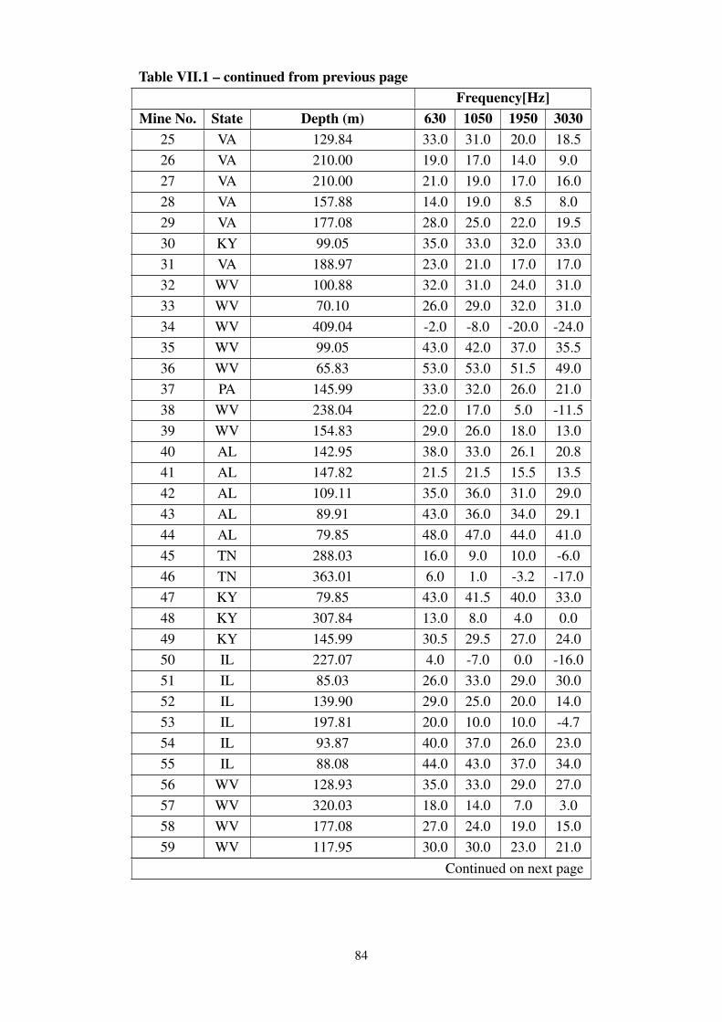
Table VII.1 – continued from previous pageFrequency[Hz]
Mine No. State Depth (m) 630 1050 1950 303025 VA 129.84 33.0 31.0 20.0 18.526 VA 210.00 19.0 17.0 14.0 9.027 VA 210.00 21.0 19.0 17.0 16.028 VA 157.88 14.0 19.0 8.5 8.029 VA 177.08 28.0 25.0 22.0 19.530 KY 99.05 35.0 33.0 32.0 33.031 VA 188.97 23.0 21.0 17.0 17.032 WV 100.88 32.0 31.0 24.0 31.033 WV 70.10 26.0 29.0 32.0 31.034 WV 409.04 -2.0 -8.0 -20.0 -24.035 WV 99.05 43.0 42.0 37.0 35.536 WV 65.83 53.0 53.0 51.5 49.037 PA 145.99 33.0 32.0 26.0 21.038 WV 238.04 22.0 17.0 5.0 -11.539 WV 154.83 29.0 26.0 18.0 13.040 AL 142.95 38.0 33.0 26.1 20.841 AL 147.82 21.5 21.5 15.5 13.542 AL 109.11 35.0 36.0 31.0 29.043 AL 89.91 43.0 36.0 34.0 29.144 AL 79.85 48.0 47.0 44.0 41.045 TN 288.03 16.0 9.0 10.0 -6.046 TN 363.01 6.0 1.0 -3.2 -17.047 KY 79.85 43.0 41.5 40.0 33.048 KY 307.84 13.0 8.0 4.0 0.049 KY 145.99 30.5 29.5 27.0 24.050 IL 227.07 4.0 -7.0 0.0 -16.051 IL 85.03 26.0 33.0 29.0 30.052 IL 139.90 29.0 25.0 20.0 14.053 IL 197.81 20.0 10.0 10.0 -4.754 IL 93.87 40.0 37.0 26.0 23.055 IL 88.08 44.0 43.0 37.0 34.056 WV 128.93 35.0 33.0 29.0 27.057 WV 320.03 18.0 14.0 7.0 3.058 WV 177.08 27.0 24.0 19.0 15.059 WV 117.95 30.0 30.0 23.0 21.0
Continued on next page
84

Table VII.1 – continued from previous pageFrequency[Hz]
Mine No. State Depth (m) 630 1050 1950 303060 WV 106.98 40.0 38.1 37.0 35.061 WV 257.86 N N N N62 WV 209.09 6.0 4.0 0.0 -6.063 WV 147.82 30.0 26.0 16.0 18.064 WV 107.89 34.0 34.0 31.0 31.065 WV 71.01 44.0 44.0 40.0 40.066 WV 78.02 16.0 17.0 15.0 16.067 WV 128.01 38.0 36.0 31.0 29.068 WV 136.85 18.2 17.6 12.1 7.969 WV 131.06 F F 32.0 25.070 WV 278.89 F F -6.0 F71 PA 72.84 54.0 52.0 43.0 39.072 PA 146.91 26.0 24.0 18.0 16.073 PA 190.80 F 26.0 21.7 F74 PA 145.99 28.0 25.0 F 15.075 PA 200.55 27.0 15.0 12.0 3.076 DT 364.84 2.4 2.0 -14.0 -24.177 DT 304.79 1.1 -0.4 -8.6 -13.878 DT 365.75 13.0 7.0 2.0 -5.079 CO 427.02 -1.6 -11.0 F F80 OH 152.39 23.9 9.0 7.0 -7.081 OH 182.87 15.0 11.0 2.0 -11.082 OH 142.95 8.0 8.0 1.0 -9.083 OH 164.89 15.0 12.0 6.0 -3.084 OH 170.99 13.0 20.0 12.0 5.085 KY 79.24 45.0 44.0 39.0 40.086 KY 152.09 26.0 24.0 18.0 14.087 KY 121.91 30.0 28.0 24.0 24.088 KY 115.82 29.0 28.0 26.0 23.089 AL 197.81 22.0 20.0 16.0 10.090 AL 472.74 -2.0 -9.0 -12.0 -16.091 KY 57.91 44.0 41.0 36.0 33.092 KY 79.85 47.5 46.5 44.0 38.093 KY 21.03 57.0 56.0 53.0 52.094 KY 99.97 27.5 20.0 7.0 -4.0
85

Table VII.2: In-mine Collins Transmitter RMS Magnetic Moment at Fundamental Operation frequency vs. Fre-quency and Depth from 94 Coal Mine SitesRMS Signal levels in dB reference (A-m2). Adapted from [48].
Frequency [Hz]Mine No. State Depth (m) 630 1050 1950 3030
1 KY 182.87 1599 1206 741 4952 KY 122.83 618 528 370 2613 KY 122.83 618 528 370 2614 IL 243.83 1438 1097 680 4565 KY 425.8 1545 1172 724 4846 KY 205.43 1545 1172 724 4847 VA 158.49 1613 1232 765 5138 KY 60.95 1410 1079 671 4509 OH 80.46 847 698 468 323
10 OH 77.41 847 698 468 32311 WV 80.46 766 619 405 27712 WV 76.19 847 698 468 32313 PA 103.93 1197 948 608 41314 PA 135.94 1264 995 635 43015 PA 182.87 931 759 502 34516 PA 210 847 698 468 32317 PA 72.84 1142 909 587 39918 PA 64 970 774 501 34119 PA 106.07 415 339 224 15420 PA 103.93 1173 931 599 40721 PA 99.05 759 631 427 29622 WV 173.43 1346 1049 663 44723 VA 365.75 1688 1279 789 52724 KY 82.29 549 474 338 24025 VA 129.84 1192 932 591 39926 VA 210 1203 952 611 41427 VA 210 1017 929 727 54628 VA 157.88 1746 1325 818 54729 VA 177.08 1727 1269 764 50730 KY 99.05 1197 948 608 41331 VA 188.97 1410 1079 671 45032 WV 100.88 1089 870 563 38333 WV 70.1 141 137 125 10834 WV 409.04 2045 1526 929 619
Continued on next page
86

Table VII.2 – continued from previous pageFrequency[Hz]
Mine No. State Depth (m) 630 1050 1950 303035 WV 99.05 1324 1037 658 44536 WV 65.83 1310 1026 651 44037 PA 145.99 1444 1119 704 47438 WV 238.04 2216 1639 992 65939 WV 154.83 1197 948 608 41340 AL 142.95 1099 870 558 37941 AL 147.82 847 698 468 32342 AL 109.11 815 672 451 31243 AL 89.91 618 528 370 26144 AL 79.85 906 741 493 33945 TN 288.03 1265 986 623 42046 TN 363.01 1123 896 580 39547 KY 79.85 639 543 379 26648 KY 307.84 1319 1020 641 43149 KY 145.99 926 755 501 34450 IL 227.07 1299 1017 646 43751 IL 85.03 718 601 410 28552 IL 139.9 858 706 471 32553 IL 197.81 1516 1169 731 49254 IL 93.87 926 756 501 34455 IL 88.08 1444 1119 704 47456 WV 128.93 855 700 466 32157 WV 320.03 1412 1081 672 45158 WV 177.08 1028 816 524 35659 WV 117.95 847 698 468 32360 WV 106.98 1025 826 540 36961 WV 257.86 936 760 501 34462 WV 209.09 936 760 501 34463 WV 147.82 1102 878 567 38664 WV 107.89 1055 846 550 37565 WV 71.01 936 760 501 34466 WV 78.02 936 760 501 34467 WV 128.01 1439 1115 701 47268 WV 136.85 847 698 468 32369 WV 131.06 1220 957 609 412
Continued on next page
87

Table VII.2 – continued from previous pageFrequency[Hz]
Mine No. State Depth (m) 630 1050 1950 303070 WV 278.89 1467 1132 709 47771 PA 72.84 1141 890 563 38072 PA 146.91 888 726 482 33173 PA 190.8 2047 1527 930 62074 PA 145.99 1324 1037 658 44575 PA 200.55 1471 1134 710 47876 UT 364.84 1031 819 527 35877 UT 304.79 1220 957 609 41278 UT 365.75 2047 1527 930 62079 CO 427.02 1342 1039 653 44080 OH 152.39 847 698 468 32381 OH 182.87 558 481 342 24382 OH 142.95 959 779 513 35283 OH 164.89 815 672 451 31284 OH 170.99 964 782 515 35385 KY 79.24 1087 871 565 38586 KY 152.09 1324 1037 658 44587 KY 121.91 1087 871 565 38588 KY 115.82 531 457 323 22989 AL 197.81 906 741 493 33990 AL 472.74 2047 1527 930 62091 KY 57.91 735 612 415 28892 KY 79.85 1324 1037 658 44593 KY 21.03 193 143 87 5894 KY 99.97 447 306 176 115
88

VIII. H-FIELD STATISTICAL DISTRIBUTIONS FORFREQUENCY AND DEPTH
0 50 100 15010
−6
10−5
10−4
Number of mine
Magnetic fie
ld A
/m
(a) H-field distribution
0 1 2 3 4 5 6 7 8
x 10−5
0
0.5
1
1.5
2
2.5
3x 10
5
Data
Pro
babili
ty d
istr
ibution
Data
Burr
GeneralizedExtremeValue
Loglogistic
(b) Statistical fitting
Figure VIII.1: H-field statistical characterization at 20 m and 657.9 Hz
89

0 50 100 15010
−6
10−5
10−4
Number of mine
Magnetic fie
ld A
/m
(a) H-field distribution
0 1 2 3 4 5 6 7 8
x 10−5
0
0.5
1
1.5
2
2.5
3x 10
5
Data
Pro
babili
ty d
istr
ibution
Data
Burr
GeneralizedExtremeValue
Loglogistic
(b) Statistical fitting
Figure VIII.2: H-field statistical characterization at 20 m and 4328.8 Hz
90

0 50 100 15010
−6
10−5
10−4
Number of mine
Magnetic fie
ld A
/m
(a) H-field distribution
0 1 2 3 4 5 6 7 8
x 10−5
0
0.5
1
1.5
2
2.5
3x 10
5
Data
Pro
babili
ty d
istr
ibution
Data
Burr
GeneralizedExtremeValue
Loglogistic
(b) Statistical fitting
Figure VIII.3: H-field statistical characterization at 20 m and 10000 Hz
91

0 50 100 15010
−10
10−9
10−8
10−7
Number of mine
Magnetic fie
ld A
/m
(a) H-field distribution
0 0.5 1 1.5 2 2.5 3 3.5
x 10−8
0
0.2
0.4
0.6
0.8
1
1.2
1.4
1.6
1.8
2x 10
8
Data
Pro
babili
ty d
istr
ibution
Data
ExtremeValue
GeneralizedExtremeValue
Weibull
(b) Statistical fitting
Figure VIII.4: H-field statistical characterization at 150 m and 657.9 Hz
92

0 50 100 15010
−10
10−9
10−8
10−7
Number of mine
Magnetic fie
ld A
/m
(a) H-field distribution
0 0.5 1 1.5 2 2.5
x 10−8
0
0.5
1
1.5
2
2.5x 10
8
Data
Pro
babili
ty d
istr
ibution
Data
Weibull
Nakagami
Beta
(b) Statistical fitting
Figure VIII.5: H-field statistical characterization at 150 m and 4328.8 Hz
93

0 50 100 15010
−11
10−10
10−9
10−8
10−7
Number of mine
Magnetic fie
ld A
/m
(a) H-field distribution
0 0.2 0.4 0.6 0.8 1 1.2 1.4
x 10−8
0
2
4
6
8
10
12x 10
8
Data
Pro
babili
ty d
istr
ibution
Data
Burr
GeneralizedPareto
Weibull
(b) Statistical fitting
Figure VIII.6: H-field statistical characterization at 150 m and 10000 Hz
94

0 50 100 15010
−11
10−10
10−9
10−8
Number of mine
Magnetic fie
ld A
/m
(a) H-field distribution
0 0.5 1 1.5 2 2.5 3 3.5
x 10−9
0
0.2
0.4
0.6
0.8
1
1.2
1.4
1.6
1.8
2x 10
9
Data
Pro
babili
ty d
istr
ibution
Data
GeneralizedExtremeValue
Beta
Burr
(b) Statistical fitting
Figure VIII.7: H-field statistical characterization at 300 m and 657.9 Hz
95

0 50 100 15010
−13
10−12
10−11
10−10
10−9
Number of mine
Magnetic fie
ld A
/m
(a) H-field distribution
0 1 2 3 4 5 6 7 8 9
x 10−10
0
0.5
1
1.5
2
2.5
3
3.5x 10
10
Data
Pro
babili
ty d
istr
ibution
Data
Lognormal
GeneralizedPareto
Burr
(b) Statistical fitting
Figure VIII.8: H-field statistical characterization at 20 m and 4328.8 Hz
96

0 50 100 15010
−14
10−13
10−12
10−11
10−10
10−9
Number of mine
Magnetic fie
ld A
/m
(a) H-field distribution
0 0.2 0.4 0.6 0.8 1 1.2 1.4 1.6 1.8 2
x 10−10
0
2
4
6
8
10
12x 10
11
Data
Pro
babili
ty d
istr
ibution
Data
Lognormal
Loglogistic
Burr
(b) Statistical fitting
Figure VIII.9: H-field statistical characterization at 300 m and 10000 Hz
97