dispersion of produced water in a coastal environment...

Continental Shelf Research 19 (1999) 57—78

Dispersion of produced water in a coastalenvironment and its biological implications

Libe Washburn!,*, Shannon Stone", Sally MacIntyre#

!Institute for Computational Earth System Science, Department of Geography, University of California,Santa Barbara, CA 93106-3060, USA

"Bermuda Biological Station for Research, 17 Biological Lane, Ferry Reach, Bermuda, GE01, USA#Marine Science Institute, University of California, Santa Barbara, CA 93106, USA

Received 20 October 1997; accepted 4 May 1998

Abstract

Produced water, a pollutant associated with offshore oil production, has been shown tohave adverse effects on marine organisms. We conducted a study of the dispersion of aproduced water plume from an outfall in the Santa Barbara Channel near Carpinteria,CA. Biological effects were studied previously in a series of experiments which examinedthe toxicity of ocean waters near the outfall. To define the changing ocean conditionsaround the outfall, we obtained time series observations of currents and water propertiesfrom July, 1992 to January, 1994. Near-field dispersion of the produced water is simulatedwith a buoyant plume model. Measured currents and density profiles are used as modelinputs. Far-field dispersion is simulated with the current statistics combined with an elementarysolution to the diffusion equation. The modeled depth of the plume varies strongly with seasondue to changing stratification. In spring and summer, the modeled plume is trapped belowthe surface. In fall and winter it extends over most of the water column and occasionallysurfaces. Minimum initial dilution is &100 in summer and &500 in winter. Far-field modelingindicates along-isobath symmetry in produced water dispersion in the mid water column.This pattern agrees with the distribution of toxic effects from the biological studies. At1000 m from the outfall, the farthest test sites in the biological studies, minimum dilutions rangefrom 4000 to 4]105 when the plume is present. These estimates exceed the threshold forsub-lethal effects found by Krause (1993) in a sea urchin fertilization bioassay. Time averageddilutions in the far-field are larger by factors of 102 to 103. ( 1998 Elsevier Science Ltd. Allrights reserved.

*Corresponding author. [email protected].

0278—4343/99/$— See front matter ( 1998 Elsevier Science Ltd. All rights reserved.PII: S0278—4343(98)00068-5

1. Introduction

Produced water, one of the most important sources of pollution associated withoil production (Stephanson, 1992), is the water extracted along with oil in thedrilling process. Large volumes of produced water are often generated becausemany oil deposits reside in or around groundwater aquifers. Produced water containsmany contaminants including hydrocarbons, heavy metals, and chemical additivessuch as corrosion inhibitors to prevent damage to refinery equipment (Higashiet al., 1992).

Following its separation from oil, produced water is often discharged directly intothe marine environment through submarine outfalls. The outfalls usually consist ofa central pipe and a diffuser; the latter constructed with tee-risers and ports throughwhich produced water is discharged. The tee-risers discharge the produced waterhorizontally in opposite directions. After discharge, produced water rises as a buoyantplume and mixes vigorously with ambient seawater. When ambient ocean waters aresufficiently stratified, the produced water rises to an equilibrium depth range where itspreads horizontally due to advection and mixing processes. When ambient watersare weakly stratified or well mixed, produced water rises to the top of the watercolumn and forms a surface plume. The diffusers are designed to maximize initialdilution (Fischer et al., 1979). Until recently it was believed that the most significantbiological impacts of produced water resulted from solids released with the discharge.These quickly settle out of the buoyant produced water plume and were thought tolimit the spatial impact of solid components in the produced water.

Recent studies show broad spatial impacts in the marine environment due to thedissolved components of produced water. In a series of experiments described byRaimondi and Schmitt (1992), Osenberg et al. (1992), Krause (1993), and Krause et al.(1992) various invertebrate species were exposed to produced water discharged froma diffuser near Carpinteria, CA. Raimondi and Schmitt (1992) exposed larvae of redabalone (Haliotis rufescens) to produced water by attaching containers of them tomoorings at 5, 10, 50, 100, 500, and 1000 m west of the diffuser and 5 and 1000 m eastof the diffuser. They showed that survivorship of pre-competent larvae (those develop-mentally incapable of settling) was inversely correlated with distance from the diffuser,both east and west. Settlement, the ability to metamorphose, and viability were alsoinversely correlated with distance when pre-competent larvae were exposed. Theseeffects extended to 100—500 m along isobaths away from the diffuser.

In another study at the Carpinteria site, Osenberg et al. (1992) found a decrease ingrowth rates along with a decline in the general condition and tissue production ofmussels (Mytilus californianus and M. edulis) at up to 1000 m from the diffuser.Patterns of sub-lethal effects were inversely correlated with distance from the diffuserand were roughly symmetric to the east and west. Densities of some benthic organisms(e.g. nematodes) increased within 100 m of the diffuser while others (e.g. polychaetes)decreased. The changes in infaunal density were also symmetric east and west of thediffuser. Osenberg et al. (1992) suggest that settling of larger particles in the producedwater or changes in sediment composition could account for the changes in infaunaldensity near the diffuser.

58 L. Washburn et al./Continental Shelf Research 19 (1999) 57—78

In laboratory experiments, adult purple sea urchins (Strongylocentrotus purpuratus)were exposed to varying concentrations of produced water from the Carpinteriadiffuser. The experiments showed that the ability of purple sea urchin sperm to fertilizeeggs was reduced for dilutions as high as 1,000,000 : 1 (Krause, 1993; Krause et al.,1992). Krause (1993) exposed purple sea urchins to samples of seawater collected atvarious distances west of the Carpinteria diffuser and found reproductive successdecreased as produced water concentration increased. Reproductive success proveduseful in inferring produced water concentration in the samples and in detectingtoxicity in the environment (Krause, 1993).

These studies are valuable but limited by the spatial and temporal scales resolved.They resolve spatial scales of 1000 m and smaller, but only at a few points and onlyalong isobaths. Thus, the effects of cross-shore dispersion cannot be examined. Theshorter duration experiments resolved temporal scales ranging from a few hours toa few days and spanning a limited range of ocean conditions. The longer durationexperiments integrated over time scales of a few months to produce single data points.Over these time scales ocean conditions change substantially. Thus, impacts due toshorter time scale processes and variable ocean conditions cannot be identified. Thesebiological studies cannot be used to examine the variations in produced waterdispersion on seasonal time scales. Nor can they resolve complex spatial patternswhich might arise from variable ocean currents and stratification. Consequently, theirusefulness in predicting the effects of produced water is limited.

Our approach to increase the predictability of these studies is to use physicaloceanographic observations to define the ambient conditions and then to simulateproduced water dispersion with a simple numerical model. Theoretical and experi-mental studies show that the structure of buoyant plumes is dependent on ambientdensity stratification and velocity field in the receiving fluid (cf. Fischer et al., 1979;Roberts et al., 1989a—c; Lee et al., 1996; Pritchard et al., 1996; List, 1982; Washburnet al., 1992; Wu et al.1994; Wu, 1993). Thus, observations of evolving stratification andcurrents around the point of discharge are critical for modeling.

We model the dispersion of produced water as a two step process. In the firststep, the buoyant plume rises and mixes with ambient seawater until it reachesan equilibrium level or the sea surface. We refer to the region in which this occursas the ‘near-field’. We simulate near-field mixing by using the buoyant plume modeldescribed by Baumgartner et al. (1994) using our time series observations of currentsand density as inputs. In a recent study by Petrenko et al. (1998), this model wassuccessful in predicting the height of rise, thickness, and initial dilution of thewastewater plume produced by the sand island treatment plant in Mamala Bay,Hawaii. The second step of the dispersion process occurs in the ‘far-field’, followingplume rise, when ambient mixing and stirring processes further dilute the plume. Wesimulate these far-field processes with the model for two-dimensional diffusion dis-cussed by Okubo (1980). Spatial patterns of produced water concentration in thefar-field are inferred from ‘visitation frequency’ diagrams constructed from currentobservations.

Our investigation is motivated by the biological studies conducted around theCarpinteria diffuser that revealed toxic effects as far as 1000 m from the outfall. An

L. Washburn et al./Continental Shelf Research 19 (1999) 57—78 59

underlying hypothesis is that these effects resulted from dissolved components whichare carried far from the point of discharge by the spreading plume. The Carpinteriaoutfall ceased operation shortly after the conclusion of the biological studies andbefore our field observations commenced. Thus, our work is retrospective andassumes that conditions during the time of our sampling represent prevailing condi-tions. Specific objectives of our study are: (1) to describe the evolving structure of thewater column and currents on seasonal time scales and shorter; (2) to use theseobservations in modeling the spatial scales of the plume; (3) to estimate dilution levelsof produced water around the diffuser; and (4) to interpret the various biological fieldassays in the light of the observations and model results.

2. Methods

2.1. Field site and instrumentation

The produced water outfall lies off the coast near the Carpinteria, CA at 34° 23@ N,119° 30.64@ W (Fig. 1). Mean water depth at the diffuser is about 12 m with a &2 mtidal variation. The diffuser, with length ¸"21 m, is at the end of the outfall pipethat extends about 300 m from the coastline. It consists of seven risers with tee-ports that extend upward off of a central pipe 0.20 m in diameter. Spacing betweentee-ports along the diffuser is 3.5 m. The tee-ports discharge effluent horizontallyinto the water column at 3.2 m s~1 through two appositely-directed nozzles,each 0.03 m in diameter. The points of discharge are about e

1"1 m above the

sea floor. Diffusers of this type are designed to produce minimum dilutions of order100 (Fischer et al., 1979). The sea floor around the diffuser is gently sloping and sandywith isobaths oriented about 100° relative to true north (Fig. 1c). About 1 km westof the diffuser is Carpinteria creek which is the discharge channel of the Carpinteriasalt marsh.

Profiles of temperature, conductivity and pressure were collected every two weeks,weather permitting, from 29 July 1992 to 4 January 1994 using a conductivity,temperature, depth profiler (CTD, Sea Cat SBE 19 manufactured by Sea-Bird Elec-tronics Inc., Bellevue WA). Thirty four profiles were obtained at the diffuser and atfour nominal locations around it: 100 m east, 100 m west, 100 m inshore, and 100 moffshore. Time-depth contours of temperature, salinity and density from all 5 locationsare very similar and only results when the diffusers are presented. Data from downcastprofiles are averaged over 0.5 decibar (dbar) and used for computing salinity anddensity. Reliable data were not consistently obtained in the upper 1 m so this portionof the water column is not included in the analysis.

Current magnitude and direction were measured by mooring two electromagneticcurrent meters (model S4, manufactured by InterOcean Inc., San Diego, CA) 25 mwest of the diffuser along the 12 m isobath. One current meter was moored 5 m fromthe bottom (approximately 7 m depth), and the other 1m from the bottom (approxim-ately 11 m depth). The upper depth was chosen to obtain data in the mid-watercolumn, but avoid heavy boat traffic in the area. Data from two different pairs of S4


Fig. 1. (a) Area map of Southern California showing field site near Carpinteria, CA. (b) Map of coastlineand watershed around the field site. (c) Field site showing produced water discharge pipe and diffuser (heavyline) and bathymetric contours (dotted lines). Dots indicate biological moorings at 100, 500 and 1000 mwest of the diffuser and 1000 m east of the diffuser.

current meters are reported. The first was deployed from 20 December 1992 to 16April 1993 and the second from 13 July 1993 until 3 January 1994. For all deploy-ments the current meters were configured to collect 2 min vector averages of currentsevery 20 min, giving a sampling frequency of f

4"72 cycles day~1. Further discussion

on the CTD, current meter, and data processing is given by Stone (1995).

2.2. Modeling near-field dispersion

In the near-field, produced water initially disperses as a rising buoyant plume whichwe simulate using the plume model described by Baumgartner et al. (1994). The modelis specifically designed to simulate buoyant plume discharge from multi-port diffusersin stratified cross flows, like the one at Carpinteria. The model (hereafter referred to asthe RSB model) is based on laboratory experiments described by Roberts et al.


(1989a—c) and on dimensional analysis. Plume dispersal was examined over a widerange of stratification conditions and current speeds using small model diffuserssimilar in configuration to the Carpinteria diffuser. Results were summarized bya series of equations with non-dimensional parameters which are used in the RSBmodel to predict plume characteristics.

Model inputs are the diffuser characteristics along with current speed and densityprofiles. For each of the 34 density profiles collected at the diffuser, we made 4 modelruns at current speeds of 0, 0.5, 0.1, and 0.2 m s~1 for a total of 136 model runs. Thechosen speeds span 99% of the range of measured current speeds. We assume thatcurrent vectors are perpendicular to the diffuser, consistent with the prevailingalong-isobath flow at the site. Density data are edited to remove inversions whichtypically occurred during periods of weak stratification and are probably instrumen-tal artifacts. Density at 10 levels is used for each model run and the water depth wasassumed constant at D"12 m.

Among the model outputs are: (1) height of the top of the plume above the dischargedepth z

%; (2) plume thickness h

%,; (3) minimum initial dilution S

.; (4) height

z.

corresponding to S.; and (5) length of the ‘initial mixing zone’ x

*(Fig. 2). These

outputs are positive and naming conventions are those used by Baumgartner et al.(1994). For graphical display of plume position in the water column we show: (1) depthof the top of the plume z

5"z

%#e

1!D; (2) depth of the bottom of the plume

zB"z

5!h

%; and (3) depth of minimum initial dilution z

#"z

.#e

1!D. The quantit-

ies z5, z

", and z

#are negative and z is positive upward from the sea surface.

The position of the plume in the water column, described by z5

and z", deter-

mines the depth interval over which organisms can be exposed to produced water.

Fig. 2. Diagram of a buoyant produced water plume released from a multi-port diffuser on the seafloor(adapted from Baumgartner et al., 1994). Produce water is discharged through tee-ports on diffuser andspreads as a buoyant plume. See text for explanation of symbols.


Stratification and current speed are primary controlling factors: weak stratificationand strong currents increase the interval while strong stratification and weak currentsdecrease it (Fischer et al., 1979, List, 1982, and Koh and Brooks, 1975). Initial dilutionS.

is a measure of the maximum produced water concentration to which organismsare exposed. Dilution is defined as the volume of a seawater sample divided by thevolume of produced water in that sample. Weak stratification and high current speedsincrease S

.; high stratification and weak currents decrease S

..

The length of the initial mixing zone x*, is the horizontal distance over which the

plume is advected by ambient currents as it rises, buoyantly mixes, and entrainsambient seawater. In laboratory experiments, Roberts et al., 1989b show that theminimum dilution over plume cross-sections increases rapidly near the diffuser. Asdistance from the diffuser approaches x

*, the turbulence in the plume quickly collapses

and further dilution due to plume-generated turbulence ceases. At distance x*away

from the diffuser, the produced water forms a passive layer within its equilibriumdepth range and the minimum initial dilution is S

.at height z

.. Within the layer

the concentration of produced water C is idealized as a Gaussian distribution(Fig. 2). Organisms residing within the plume in the initial mixing zone are exposed tohighly variable concentrations of produced water due to strong turbulence. Dilutionlevels can be less than S

.within this zone. Beyond x

*the plume moves into the

‘far-field’.

2.3. Modeling far-field dispersion

After the initial mixing during plume rise, ambient ocean mixing processes furtherdilute the produced water plume and alter its width and height. These complexprocesses include small-scale turbulent mixing, shear dispersion, and horizontalmixing. In addition, the width of the plume slowly increases and the thicknessh%

slowly decreases due to gravitational collapse of the plume into the stratifiedsurroundings (Roberts et al., 1989b). We do not have sufficient measurements toestablish the details of how these processes affect the plume. However, we can examinethe net effects of these processes on dilution through a simple horizontal diffusionmodel. In doing so, we assume that horizontal mixing processes are dominant andthat the complex dispersion processes can be parameterized by a horizontal eddydiffusivity k

H. Clearly this is an over simplification. The objective here is only to

establish the order of magnitude of additional dilution in the far field.We estimate the far-field dilution with an elementary solution of the two-dimen-

sional diffusion equation. The plume in the far-field is idealized as consisting ofa sequence of cylindrical patches of produced water that continuously expand due totwo-dimensional mixing processes. The patches move along horizontal trajectoriesdefined by progressive vector diagrams (PVDs) that are obtained from currentmeasurements. PVDs are idealizations of real trajectories since they assume a ‘frozen’velocity field (equivalent to the ocean moving as a slab). Nevertheless, they are usefulin predicting displacements of water parcels from single point current measurements.We employ ‘visitation frequency diagrams’ (described below), formed from the PVDs,to examine the spatial distribution of produced water around the diffuser.


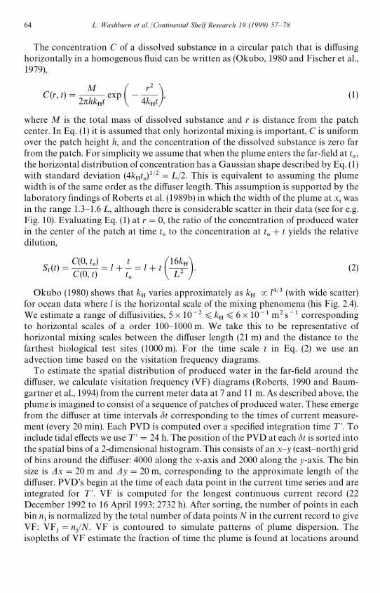
The concentration C of a dissolved substance in a circular patch that is diffusinghorizontally in a homogenous fluid can be written as (Okubo, 1980 and Fischer et al.,1979),

C(r, t)"M

2nhkHtexp A!

r2

4kHtB, (1)

where M is the total mass of dissolved substance and r is distance from the patchcenter. In Eq. (1) it is assumed that only horizontal mixing is important, C is uniformover the patch height h, and the concentration of the dissolved substance is zero farfrom the patch. For simplicity we assume that when the plume enters the far-field at t

0,

the horizontal distribution of concentration has a Gaussian shape described by Eq. (1)with standard deviation (4k

Ht0)1@2"¸/2. This is equivalent to assuming the plume

width is of the same order as the diffuser length. This assumption is supported by thelaboratory findings of Roberts et al. (1989b) in which the width of the plume at x

*was

in the range 1.3—1.6 ¸, although there is considerable scatter in their data (see for e.g.Fig. 10). Evaluating Eq. (1) at r"0, the ratio of the concentration of produced waterin the center of the patch at time t

0to the concentration at t

0#t yields the relative

dilution,

S&(t)"

C(0, t0)

C(0, t)"l#

t

t0

"l#t A16k

H¸2 B . (2)

Okubo (1980) shows that kH

varies approximately as kHJl4@3 (with wide scatter)

for ocean data where l is the horizontal scale of the mixing phenomena (his Fig. 2.4).We estimate a range of diffusivities, 5]10~2)k

H)6]10~1 m2 s~1 corresponding

to horizontal scales of a order 100—1000 m. We take this to be representative ofhorizontal mixing scales between the diffuser length (21 m) and the distance to thefarthest biological test sites (1000 m). For the time scale t in Eq. (2) we use anadvection time based on the visitation frequency diagrams.

To estimate the spatial distribution of produced water in the far-field around thediffuser, we calculate visitation frequency (VF) diagrams (Roberts, 1990 and Baum-gartner et al., 1994) from the current meter data at 7 and 11 m. As described above, theplume is imagined to consist of a sequence of patches of produced water. These emergefrom the diffuser at time intervals dt corresponding to the times of current measure-ment (every 20 min). Each PVD is computed over a specified integration time ¹@. Toinclude tidal effects we use ¹@"24 h. The position of the PVD at each dt is sorted intothe spatial bins of a 2-dimensional histogram. This consists of an x—y (east—north) gridof bins around the diffuser: 4000 along the x-axis and 2000 along the y-axis. The binsize is Dx"20 m and Dy"20 m, corresponding to the approximate length of thediffuser. PVD’s begin at the time of each data point in the current time series and areintegrated for ¹@. VF is computed for the longest continuous current record (22December 1992 to 16 April 1993; 2732 h). After sorting, the number of points in eachbin n

+is normalized by the total number of data points N in the current record to give

VF: VF+"n

+/N. VF is contoured to simulate patterns of plume dispersion. The

isopleths of VF estimate the fraction of time the plume is found at locations around


the diffuser. For each bin, the mean advection time t+from the diffuser to the bin is also

computed. t+is used as the time scale t in Eq. (2) to compute S

&(t) around the diffuser.

3. Results

3.1. Water column evolution and near-shore currents

The CTD observations at the diffuser show two distinct thermal regimes throughthe year: (1) the summer regime from May through September, characterized bystrong thermal stratification; (2) the winter regime from October to April, character-ized by weak thermal stratification (Fig. 3a). The water column was thermally

Fig. 3. Time-depth contours of (a) temperature (contour interval is 0.5°C), (b) salinity (contour interval is0.2 between solid lines; additional contours shown as dashed lines), (c) potential density anomaly ph(contour interval is 0.2 kg m~3). Shaded areas are warmest temperatures, lowest salinities, and lowestdensities. Arrows along the upper axis in each panel show the times of CTD casts. Data were not reliablycollect in the upper 1 dbar and results are not shown here.


stratified when our measurements commenced on 29 July 1992. Cooling beganin September, but thermal stratification persisted throughout the month. Bymid-October thermal stratification weakened as the water column became nearlyisothermal. Salinity decreased slightly to 33.2 psu during this period, indicatingadvection of a new water mass (this change is not resolved by contours spacingof Fig 3b). Between sampling on 27 October 1992 and 22 December 1992, the watercolumn cooled from 18°C to 14°C and the potential density anomaly (ph) increasedfrom about 24.2 kgm~3 to 24.6 kgm~3 (Fig. 3c). Winter rainfall produced largeincrease in density stratification at the field site (Fig. 3c) with layering of fresh watermost prominent in January, February, and March, 1993 (shaded areas, Fig. 3b).During these times moderate stratification prevailed even though the water columnwas nearly isothermal (Fig. 3a). On 20 January, 1993, for example, ph increased from23.130 kg m~3 at 1 dbar to 23.795 kg m~3 at 11 dbar. The mean buoyancy frequencythen was N"13.2 cycles/h (cph) where,

N"C!g

oLoLzD

1@2"C!

g

oDoDzD

1@2. (3)

g is the gravitational acceleration, o is seawater density, and z is positive upwards. N iscomputed from the density difference Do over the entire measurement depth Dz,typically 11 m.

After the period of rainfall, weaker thermal stratification prevailed until June, 1993when stratification increased. The maximum stratification observed occurred on 21June 1993 when the temperature varied from 18.6°C at 1 m to 15.9°C at 11 m withN"22 cph. Strong thermal stratification persisted until October, 1993 when thewater column cooled and became more uniform. By 11 October 1993, the watercolumn was nearly isothermal again with a temperature of 17.5°C. In November andDecember the water column remained nearly isothermal and cooled from 16°C to lessthan 15°C.

Currents are highly variable at the field site throughout the year and at bothmeasurement depths, nominally 7 and 11 m (Fig. 4). However, no clear seasonaltrend in currents is found in our records. Sub-tidal currents show low frequencyevents in which currents are fairly steady for periods of a few days (data notshown). Little coherence is evident between sub-tidal current velocity at 7 and 11 mand large differences in speed and direction frequently occur. A representativesubset of the current data (Fig. 4) shows periodicity in the current time seriesresulting primarily from the semi-diurnal, lunar (M

2) tide. Power spectra of current

speed at 7 and 11 m show clear peaks at the M2

frequency (data not shown).Nearshore current observations from other locations in the Southern California Bightalso show the dominance of the M

2tide. For example, Winant and Olson (1976)

reported 0.1 m s~1 along-shore currents due to the M2

tide at 18 m depth offDel Mar, CA.

Histograms of current direction at 7 and 11 m exhibit very different distributions.At 7 m the histogram of current direction has two clearly defined peaks, one around100° and another around 280° (Fig. 5a). These directions are approximately parallel to


Fig. 4. Needle plots of current magnitude and direction at 7 m (upper time series) and 11 m (lower timeseries) for 16—20 November 1993. Each needle represents a 2 min vector average of a current velocity andneedles are 20 min apart. Speed scale shown in upper right corner.

depth contours (Fig. 1c) and indicate along-isobath flow. At 11 m the histogramexhibits a single broad maximum at around 270° (Fig. 5b) and no clear peak is foundaround 100°. Totals in bins at 0, 90, 180, 270 degrees have been set to zero in thehistograms of Fig. 5. Anomalous high values in these bins result from uncertainties incurrent direction at speeds of less than 2 cm s~1 (Stone, 1995). Table 1 shows that theflow distributions sorted by quadrant change significantly between 7 and 11 m.Southward (cross-isobath) flow is much more common at 11 m (28.8% of record) thanat 7 m (8.3%). Westward flow occurs most frequently at both depths: for 33.7% of the11 m record and for 43.4% of the 7 m record.

Given the high variability in current speed, the produced water plume can besignificantly affected by currents. The effects of currents may be parameterized by theFroude number for buoyant plumes (Fischer et al., 1979),

F"

u3

b, (4)

where u is current speed and b is the specific buoyancy flux. Specific buoyancy flux is,

b"g(o

0!o

%)

o0

Q

¸

, (5)

where o0is ambient density, o

%is produced water density, and Q is volume flux from

the diffuser. F is the ratio of the flux of kinetic energy of the mean flow to the buoyancyflux of the plume. High values of F lead to a diffuse plume because currents mix moreambient fluid into the plume (Fischer et al., 1979, Roberts et al., 1989a). Low values ofF result in a more concentrated plume because advection is weaker and less ambient


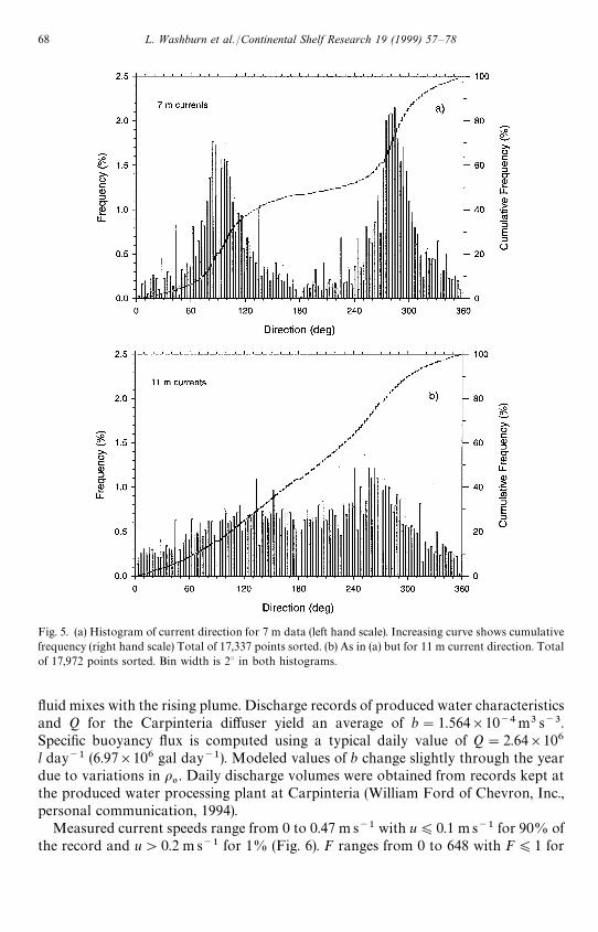
Fig. 5. (a) Histogram of current direction for 7 m data (left hand scale). Increasing curve shows cumulativefrequency (right hand scale) Total of 17,337 points sorted. (b) As in (a) but for 11 m current direction. Totalof 17,972 points sorted. Bin width is 2° in both histograms.

fluid mixes with the rising plume. Discharge records of produced water characteristicsand Q for the Carpinteria diffuser yield an average of b"1.564]10~4m3 s~3.Specific buoyancy flux is computed using a typical daily value of Q"2.64]106l day~1 (6.97]106 gal day~1). Modeled values of b change slightly through the yeardue to variations in o

0. Daily discharge volumes were obtained from records kept at

the produced water processing plant at Carpinteria (William Ford of Chevron, Inc.,personal communication, 1994).

Measured current speeds range from 0 to 0.47 m s~1 with u)0.1 m s~1 for 90% ofthe record and u'0.2 m s~1 for 1% (Fig. 6). F ranges from 0 to 648 with F)1 for


Table 1Current statistics at the Carpinteria site

7 m currents 11 m Currents

Quadrant Direction No. % of speed No. % of speed(deg) observations record (ms~1) observations record (ms~1)

East 45—135 6607 38.1 0.05 4575 25.5 0.05West 225—315 7522 43.4 0.06 6060 33.7 0.05South 135—225 1442 8.3 0.02 5178 28.8 0.04North 315—45 1766 10.2 0.02 2159 12.0 0.03

Total 17337 100 17972 100

Fig. 6. Histogram (solid line, left hand scale) and cumulative distribution (dashed line, right hand scale) ofcurrent speed u at 7 m. Upper scale shows corresponding values of Froude number F"u3b~1 based on themean specific buoyancy flux b"1.56]10~4m3 s~3.

68% of the record and F'10 for 5%. For F)0.1, about 33% of the record,the plume structure is similar to that found in a stationary environment (Robertset al., 1989a). Similar ranges of u and F are found at 11 m (data not shown). The broadrange of F indicates that the plume structure changes depending on the currentregime.


3.2. Near-field mixing

The modeled position of the plume in the water column is strongly modulated bychanging stratification through the year (Fig. 7a—c). This occurs for all modeledcurrent speeds and the results of Fig. 7 for 0 and 0.1 m s~1 are representative. Themodeled plume is lowest (minimum z

5) and thinnest (minimum z

5!z

") during the

periods of highest stratification in summer. For 1993 this happens in June whenz5"!6.5 m and z

5!z

""2.6 m. The depth of the bottom of the plume z

"is more

constant than z5due to entrainment of deeper, denser waters. It is always more than

7 m from the surface, but seldom within 2 m of the bottom. The depth of minimuminitial dilution lies above the mid-point of the plume and its depth varies more thanz5and less than z

". In the period January through March, 1993 the plume depth first

decreases, then increases, and then decreases again due to changing salinity stratifica-tion from rainwater runoff (Fig. 3).

The effect of current speed on plume depth is clearly evident: at zero current speedthe plume rises higher into the water column at all stratifications. In late fall and early

Fig. 7. Near-field modeling of produced water plume. Panels show outputs from RSB plume model based ontime series of density shown in Fig. 3c. (a) Plume depths with u"0 ms~1. Lower solid line shows bottom ofplume (z

"), upper solid line shows top of plume (z

5), and dashed line shows depth of minimum dilution (z

#). (b)

As in (a) but for u"0.1 ms~1. (c) Minimum dilution in plume at current speeds of 0 m s~1 (lower curve) and0.1 ms~1 (upper curve). (d) Length of initial mixing zone for 0 m s~1 (lower curve) and 0.1 m s~1 (upper curve).


winter (October into December) the plume surfaces and occupies most of the watercolumn for u"0 (Fig. 7b). A shorter period of plume surfacing occurs in April andMay, 1992. At u"0.1 m s~1, z

5is deeper in the water column and the plume surfaces

for shorter periods in winter (Fig. 7c). Overall, however, the effects of currents are lessimportant in controlling the plume height than stratification.

Another consequence of changing stratification and current speed is that theminimum initial dilution S

.is highly variable. When stratification is high in summer

and after rain events in winter, the plume is mixed over less of the water column(reduced z

5!z

") resulting in lower values of S

.. For example, with u"0, S

."50 in

mid-June 1993 (Fig. 7d); with u"0.1 m s~1, S."100 at this time. For periods of

weaker stratification in fall and winter, the plume mixes over more of the watercolumn and S

.is higher. At these times, maximum S

.+150 for u"0 and S

.+500

for u"0.1 m s~1.The extent of the initial mixing zone x

*is a strong function of both current speed

and stratification (Fig. 7e). For u"0, x*

is fairly constant at 10 m or less. Atu"0.1 m s~1, x

*varies from a minimum of about 20 m in summer to over 80 m in

winter. Freshwater stratification from winter storms reduces x*to around 30 m on

time scales of less than a few weeks. After the storms, x*

quickly increases asstratification decreases.

3.3. Far-field mixing

The VF diagram computed from currents at 7 m indicates a strong tendency for theproduced water plume to advect along shore (i.e. follow isobaths) in mid-watercolumn (Fig. 8a). The pattern of isopleths is roughly symmetric along shore and acrossshore, but the along-shore scale of the pattern is about six times the cross-shore scale.At 11 m the along-shore scale of isopleths is reduced compared with 7 m and thepattern is displaced offshore (Fig. 8b). The pattern indicates that produced water nearthe bottom would frequently advect offshore, toward the southwest. The presence ofnon-zero values inshore of the coastline is an artifact of the assumption of frozen flow.Velocity gradients may exist inshore of the current meter positions and are notrepresented in the PVD’s.

Dilution in the far-field ranges from minimum values, which we can estimate, toessentially infinite values when uncontaminated seawater is present. We estimate thetotal far-field dilution at 7 m when the plume is present by,

SDt"S

.S&, (6)

where subscript Dt denotes that the plume is present for time Dt out of a total recordlength ¹. Advection time t, used for computing S

&from Eq. (2), ranges from &3 h at

100 m from the diffuser to 10—12 h at 1000 m (contours of t not shown). Lowest SDtis

likely in summer when S.

is small. Assuming minimum S.+50 (Fig. 7d) and low

kH+0.05 m2 s~1, SDt

ranges from 500 for the mooring 100 m west of the diffuser to3000—4000 at the 1000 m moorings (Fig. 9A). During weakly stratified conditionscommon in winter, SDt

is much higher: with S.+500 (Fig. 7d) and high


Fig. 8. (a) Diagram of visitation frequency VF indicating fraction of time that plume is present at locationsaround the diffuser. VF computed from currents at 7 m. Only values above 0.003 are shown and thoseabove 0.007 are shaded. Plus signs (#) show locations of biological moorings 100, 500 and 1000 m west ofthe diffuser and 1000 m east of the diffuser. Location of produced water diffuser indicated by white dot incenter of pattern. Coast line indicated with heavy solid line. (b) As in (a) but for VF computed from currentsat 11 m.

kH+0.6 m2 s~1, SDt

at the moorings is 1—5]105 (Fig. 9B). We have no data indicatinga seasonal dependence of k

H. However, we use a low and high values for summer and

winter conditions to determine the maximum range in expected dilution. Clearly,uncertainty in k

His an important source of error in these dilution estimates.

Time-averaged dilution STis much higher than SDt

because the plume is not presentat any point in the far-field for all ¹. Following Fischer et al. (1979), S

Tis obtained


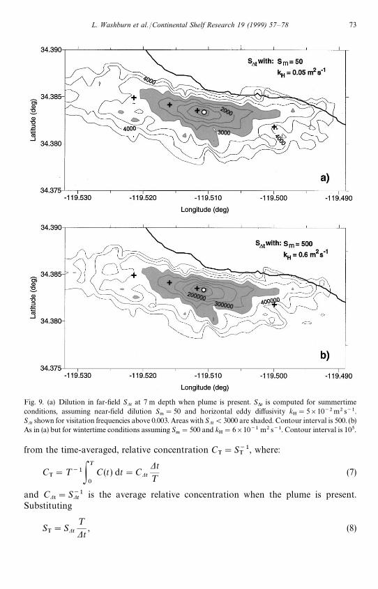
Fig. 9. (a) Dilution in far-field SDtat 7 m depth when plume is present. S*t is computed for summertime

conditions, assuming near-field dilution S."50 and horizontal eddy diffusivity k

H"5]10~2m2 s~1.

SDtshown for visitation frequencies above 0.003. Areas with SDt

(3000 are shaded. Contour interval is 500. (b)As in (a) but for wintertime conditions assuming S

."500 and k

H"6]10~1 m2 s~1. Contour interval is 105.

from the time-averaged, relative concentration CT"S~1

T, where:

CT"¹~1P

T

0

C(t) dt"CDt

Dt

¹

(7)

and CD5"S~1Dt

is the average relative concentration when the plume is present.Substituting

ST"SDt

¹

Dt, (8)


Fig. 10. (a) Time-averaged dilution in far-field ST

at 7 m depth. ST

is computed for summertime conditions,assuming near-field dilution S

."50 and horizontal eddy diffusivity k

H"5]10~2m2 s~1. S

Tshown for

visitation frequencies above 0.003. Time-averaged dilutions for wintertime conditions are 1—2 orders ofmagnitude larger (not shown).

we estimate STfrom SDt

(Fig. 9) with *t/¹ approximated by the visitation frequency at7 m (Fig. 8a). The resulting spatial distributions of S

Tvary widely within 1000 m of the

diffuser (Fig. 10). For summertime conditions and low kH, S

Tranges from 3]104 at

100 m from the diffuser to 5—7]105 at 1000 m (Fig. 10). For wintertime conditionsST

is much higher: ST&106 at 100 m from the diffuser and S

T&108 at 1000 m (not

shown).

4. Discussion

Results from our study of produced water dispersion are consistent with resultsfrom the biological studies conducted at the Carpinteria site. Raimondi and Schmitt(1992) found that larvae of red abalone were adversely affected by proximity to thediffuser at all depths tested (1.5 m from surface and 1.5 m from bottom). Because theirexperiments were conducted in October when stratification is weak, it is likely thatproduced water extended over most of the water column (Fig. 7b and c). Surfacing ofthe plume also occurs in October based on our modeling. Thus, it would be expectedthat larvae moored near the surface around the diffuser would be exposed frequentlyto produced water.

The decrease in toxic effects away from the diffuser is consistent with the decrease inVF (Fig. 8a), increased SDt

(Fig. 9), and increased ST

(Fig. 10). Moorings of Raimondiand Schmitt (1992) at 5, 10, and 50 m were often within the modeled initial mixingzone which typically extends 10—80 m away from the diffuser (Fig. 7e). Organisms in


the initial mixing zone would experience highly variable dilution levels due to mixingprocesses in the rising plume. Instantaneous dilution could often be much less thanS.

of Fig. 7d. This may account for the 50% survivorship of pre-competent larvaewithin 10 m of the diffuser and a 70% survivorship at 100 m. The isopleths of VF at7 m suggest that the mooring 100 m west of the diffuser is exposed to produced waterabout 5 times more frequently than the mooring at 500 m and &7 times more thanthe one at 1000 m (Fig. 8a). The east—west symmetry in the pattern of toxic effectsnoted by Raimondi and Schmitt (1992) agrees with the symmetric pattern of visitationfrequency of Fig. 8a.

The toxic effects near the bottom found by Raimondi and Schmitt (1992) appear tocontradict some the model results for near-field dispersion of the plume. In Figs. 7band c the base of the plume is seldom within 2 m of the bottom, so organisms at 1 mwould not necessarily be exposed to the produced water. However, we speculate thatthe turbulent bottom boundary layer may often extend into the plume. Under thesecircumstances, produced water could be entrained and mixed downward below theplume’s equilibrium depth range. Alternatively, at high current speeds in the ‘forcedentrainment’ regime (Roberts et al., 1989a), the base of the plume remains at the portdepth (1 m) over the entire initial mixing zone. When this happens, organisms1 m above the bottom and within the initial mixing zone would be exposed directly toproduced water. Roberts et al. (1989b) found that the minimum value of Fr corres-ponding to forced entrainment occurs somewhere in the range 1(Fr(10. Based onour measured current speeds, the forced entrainment regime prevails 5—32% of thetime at the Carpinteria site.

Osenberg et al. (1992) found that sub-lethal effects on mussels and pre-competentlarvae increased with proximity to the diffuser and exhibited east—west symmetry.Again, the patterns are consistent with our results. The mussels were placed 4.5 mabove the bottom, a depth almost always within the equilibrium depth range of theplume (Fig. 7b and c). Thus, very frequent exposure to produced water could occur,particularly for moorings near the diffuser. Exceptions would be during very briefperiods of strong stratification and high currents when the plume is deeper in thewater column (e.g. June 1993, Figs. 7b and c). Under stratified conditions, common insummer when the plume is trapped at depth, organisms near the surface would not beexposed to produced water, even directly over the diffuser.

These model results support the conclusion of Krause (1993) that the plume extendsat least 1000 m from the diffuser. They also suggest that measurable toxic effects mayextend beyond 1000 m from the diffuser. Krause (1993) derived a profile of producedwater concentration west of the diffuser based on toxicity. From samples collected inMay, 1991 at 1000 m west of the diffuser, he estimated a relative concentration of2]10~6, equivalent to a dilution of 5]105. This is close to the (very broad) range ofSDt

from our modeling (Fig. 9): at 1000 m west of the diffuser SDtis 4]103—4]105,

depending on S.

and kH. Krause (1993) found up to a 10% reduction in the

fertilization of purple sea urchin eggs when sperm were exposed to produced waterconcentrations as low as 0.0001% (relative dilution of 106). Based on our modeling,SDt

typically exceeds this threshold (Fig. 9). During periods of high stratificationcommon in summer, S

Talso exceeds this threshold (Fig. 10). For conditions of weak


stratification common in winter, ST

is &106 at 100 m and much larger beyond, sotoxic effects are likely to be less widespread.

Our results suggest the following predictions concerning the spatial distribution ofproduced water at the Carpinteria site:1. East—west (along-isobath) symmetry in the distribution of produced water is

maintained throughout the year in the mid and upper water column.2. The spatial scale of the along-shore distribution of produced water is about 6 times

the cross-shore scale in the mid and upper water column.3. Cross-shore asymmetry in the distribution of produced water occurs near the

bottom where the produced water extends southward (across isobaths) from thediffuser.

4. Exposure to produced water will vary strongly with depth in spring—summer andvary weakly with depth in fall-winter.While the existing biological observations are valuable, they cannot be used to test

these predictions. The experiments of Raimondi and Schmitt (1992) were conductedonly during periods of weak stratification and were of limited duration (a few hours toa few days). Those of Osenberg et al. (1992) were longer in duration, since theyspanned summer-fall (June—October, 1990), but are unable to resolve temporal vari-ations smaller than the experimental period. Experiments of Krause et al. (1992) andKrause (1993) also were of limited duration and did not resolve seasonal changes.

5. Conclusions

We conducted a combined field and modeling study to investigate the dispersion ofproduced water around a diffuser near Carpinteria, California. Observations ofcurrents and water properties were used as inputs for a model of buoyant plumedispersal. The model simulated the dispersion and spatial distribution of producedwater in the near-field around the diffuser. Far field dispersion was simulated using anelementary solution to the diffusion equation in combination with the current obser-vations.

The observations show that strong thermal stratification prevails in spring andsummer and weak stratification in fall and winter. No seasonal trend in currents isfound. Currents at mid-depth flow along isobaths while those near the bottomfrequently have an offshore, cross-isobath component. For 90% of the observations,currents speeds are 0.1 m s~1 or less.

A primary factor controlling the exposure of organisms to produced water aroundthe diffuser is the depth range of the plume in the water column. The plume depth ismodulated by seasonal changes in stratification. The plume is trapped below thesurface in spring and summer and intermittently in winter due to freshening by winterstorms. In fall and winter, it is mixed vertically through most of the water column.

Visitation frequency diagrams, constructed from current observations, indicate thatproduced water distributions exhibit east—west (along-isobath) symmetry in the mid-water column. This symmetry is in qualitative agreement with results from biologicalstudies investigating the along-shore pattern of produced water impacts on various


invertebrate species. Near the bottom the pattern of visitation frequency indicates thatthe produced water distributions are displaced offshore.

Initial dilution of produced water in the near-field depends on stratification andcurrent speed. Minimum values of order 50—100 occur in summer with strongstratification and low current speed; maximum values of 500 occur in winter for lowstratification and higher speeds (order 0.1 m s~1). These represent the maximumconcentrations to which organisms are generally exposed in the near field. Higherconcentrations are possible in the initial mixing zone extending up to &80 m fromthe diffuser.

Because of mixing processes and variable currents, dilution in the far-field is muchhigher than initial dilution. However, far-field dilutions are poorly constrained due touncertainties in ambient mixing rates. We estimate that within 1000 m of the diffuser(along-shore), ambient mixing processes increase dilution by factors of order 10 to 103when the plume is present in the far field. Because the plume is not always present atany given point, time-averaged dilutions are larger still by factors of 102—103. Ourresults support the conclusion of Krause (1993) that toxic effects are detectable at least1000 m from the diffuser.

Acknowledgements

We thank Anne Petrenko and Brian Emery for helpful comments on an early draftof the manuscript. We also thank William Ford of Chevron, Inc. for providingdetailed information about the diffuser and produced water discharge at the Carpin-teria site. Krisada Lertchareonyong provided valuable assistance with programming.We thank Chris Gotshalk for help with field work. This research was funded by theUC Coastal Toxicology Program and by the Minerals Management Service, USDepartment of Interior under MMS Agreement No. 14-35-0001-3071. The view andconclusions in this paper are those of the authors and should not be interpreted asnecessarily representing the official policies, either expressed or implied, of the USGovernment.

References

Baumgartner, D.J., Frick, W.E., Roberts, P.J.W., 1994. Dilution Models for Effluent Discharges, 3rd ed. USEnvironmental Protection Agency Report no. EPA/600/R-94/086, Washington, DC.

Fischer, H.B., List, E.J., Koh, R.C.Y., Imberger, J., Brooks, N.H., 1979. Mixing in Inland and CoastalWaters. Academic Press, New York.

Higashi, R.M., Cherr, G.N., Bergens, C.A., Fan, T.-W.M., 1992. An approach to toxicant isolation froma produced water source in the Santa Barbara Channel, In: Ray, J.P., Engelhardt, F.R., (Eds.), ProducedWater: Technological/Environmental Issues and Solutions. Plenum Press, New York pp. 223—233.

Koh, C.Y., Brooks, N.H., 1975. Fluid mechanics of waste-water disposal in the ocean. Annual Reviews inFluid Mechanics 7, 187—211.

Krause, P., 1993. Effects of poduced water on reproduction and early life stages of the purple sea urchin(Strongylocentrotus Purpuratus): field and laboratory tests. Ph.D. Dissertation, UCSB, 140 p.


Krause, P.R., Osenberg, C.W., Schmitt, R.J., 1992. Effects of produced water on early life stages of a seaurchin: stage-specific responses and delayed expression. In: Ray, J.P., Engelhardt, F.R., (Eds.), ProducedWater: Technological/Environmental Issues and Solutions. Plenum Press, Newyork pp. 431—444.

Lee, R.S., Pritchard, T.R., 1996. Dispersion of effluent from Sydney’s new deepwater outfalls, Part 1: Oceanprocesses, In: Pttiaratchi, C. (Ed.), Coastal and Estuarine Studies. American Geophysical Union,Washington, DC, 430—438.

List, E.J., 1982. Turbulent jets and plumes. Annual Reviews in Fluid. Mechanics 14, 189—212.Okubo, A., 1980. Diffusion and Ecological Problems: Mathematical Models. Springer,Berlin 254pOsenberg, C.W., Schmitt, R.J., Holbrook, S.J., Canestro, D., 1992. Spatial scale of ecological effects

associated with an open coast discharge of produced water. In: Produced Water: Technological/Environ-mental Issues and Solutions. Plenum Press, New York, pp. 387—402.

Petrenko, A.A., Jones, B.H., Dickey, T.D., 1998. Shape and near-field dilution of the Sand Island sewageplume observations compared to model results. Journal of Hydraulic Engineering, 124, 565—571.

Pritchard, T.R., Lee, R.S., Davison, A., 1996. Dispersion of effluent from Sydney’s new deepwater outfalls,Part 2: Observations of plume behaviour: winter and summer examples. In: Pttiaratchi, C. (Ed.), Coastaland Estuarine Studies. American Geophysical Union, Washington, DC, pp. 439—452.

Raimondi, P.T., Schmitt, R.J., 1992. Effects of Produced Water on Settlement of Larvae: Field Tests UsingRed Abalone. In: Produced Water: Technological/Environmental Issues and Solutions. Plenum Press,New York, pp. 415—430.

Roberts, P.J.W., 1990. Outfall design considerations, In: Le Mehaute, B., Hanes, D.M. (Eds.), The Sea,Ocean Engineering Science. Wiley InterScience, New York.

Roberts, P.J.W., Snyder, W.H., Baumgartner, D.J., 1989a. Ocean outfalls. I: submerged wastefield forma-tion, Journal of Hydraulic Engrineering 115, 1—25.

Roberts, P.J.W., Snyder, W.H., Baumgartner, D.J., 1989b. Ocean outfalls. II: spatial evolution of submergedwastefield. Journal of Hydraulic Engineering 115, 26—48.

Roberts, P.J.W., Snyder, W.H., Baumgartner, D.J., 1989c. Ocean outfalls. III: effect of diffuser design on thesubmerged wastefield. Journal of Hydraulic Engineering 115, 49—70.

Stephenson, M.T., 1992 A survey of produced water studies, In: Ray, J.P., Engelhardt, F.R. (Eds.), ProducedWater: Technological/Environmental Issues and Solutions. Plenum Press, New York, pp. 1—11.

Stone, S., 1995. Spatial scale of produced water impacts as indicated by plume dynamics and biological fieldassays. Masters Thesis, University CA. Santa Barbara.

Washburn, L., Jones, B.H., Bratkovich, A., Dickey, T.D., Chen, M.S., 1992. Mixing, dispersion, andresuspension in the vicinity of an ocean wastewater plume. Journal of Hydraulic Engineering 118 (1),38—58.

Winant, C.D., Olson, J.R., 1976. The vertical structure of coastal currents. Deep-Sea Research, 23, 925—936.Wu, Y., 1993. The study of an ocean outfall buoyant plume near Whites Point, California. Ph.D.

Dissertation, University of Southern California.Wu, Y., Washburn, L., Jones, B.H., 1994. Buoyant plume dispersion in a coastal environment: Evolving

plume structure and dynamics. Continental Shelf Research 14, 1001—1023.


dispersion of produced water in a coastal environment...

Documents