dispersion of 5 mhz zero sound in superfluid he near t [subscript...
TRANSCRIPT

DISPERSION OF 5 MHZ ZERO SOUND
IN SUPERFLUID 3He
NEAR T IN MAGNETIC FIELDSc
By
ROBERT FRANK BERG
A DISSERTATION PRESENTED TO THE GRADUATE SCHOOL
OF THE UNIVERSITY OF FLORIDA IN
PARTIAL FULFILLMENT OF THE REQUIREMENTS
FOR THE DEGREE OF DOCTOR OF PHILOSOPHY
UNIVERSITY OF FLORIDA
1983

ACKNOWLEDGEMENTS
It is only with the skillful guidance of my research advisor,
Professor Gary Ihas , that I have been able to pursue and complete a
program of doctoral research at the University of Florida. He has been
both mentor and friend, offering critical advice and encouragement
whenever it was needed. I hope that his investment of many long nights
and days in the laboratory with me has proved as rewarding to him as it
has to me. I also owe a great debt to Professor Hugh G. Robinson of
Duke University for the year of training and support I received in his
laboratory and for his understanding and encouragement upon my transfer
to Florida.
In addition to provessor Ihas, many people associated with the
Department of Physics at U.F. have contributed their time and energy to
help me. Chief among them is Professor Dwight Adams, whose advice and
material assistance have proved invaluable on many occasions. Conversa-
tions with and assistance from Dr. Kurt Uhlig, Dr. Vijay Samalam, Greg
Haas, John Polley, Tang Yi-Hua, Greg Spencer, and Brad Engel have been
an enjoyable part of my stay here at U.F. Brad Engel also helped in
taking the latter portion of the data for this thesis. The expert
technical assistance of Christian Fombarlet, Don Sanford, James
Robinson, and the men in the machine shop under Harvey Nachtrieb has
been unfailing. Sheri Hill is thanked for the skillful typing of this
manuscript.

Three women in my life have been of utmost importance to me.
My mother, Dr. Ernestine Berg, whose example and attitude led me to an
appreciation of science, has always believed in me . My aunt, Dr.
Pauline Billiard, has given her support during my stay in Gainesville,
especially during the last five months. My wife, Dr. Carol Emerson, is
owed thanks for her patience and understanding during these years and
also for leading me into low temperature physics in the first place.
Funding for this project has been supplied by the Division of
Sponsored Research at U.F. and the National Science Foundation (DMR-
8006929 and DMR-8306579)
.

TABLE OF CONTENTS
ACKNOWLEDGEMENTS .' ii
TABLE OF CONTENTS iv
LIST OF FIGURES vi
ABSTRACT ix
SECTION 1 INTRODUCTION 1
SECTION 2 PERTINENT THEORY OF 3He 15
2 .
1
General References 15
2 . 2 The Normal Fermi Liquid 15
2.3 Superfluid Pairing 182.4 Comparison of the ABM and BW States 202.5 Strong Coupling and the Finite
Field Phase Diagram .'. 23
2.6 NMR in the A and Al Phases 27
2.7 Sound Propagation in the NormalFermi Liquid and the ABM-State 32
SECTION 3 APPARATUS 51
3 .
1
Large-Scale Features 51
3.2 Dilution Refrigerator 553.3 Nuclear Cooling Stage 593.4 Bundle Construction 61
3.5 Thermal Isolation and Heat Leaks 65
3.6 Superfluid-Handling Apparatus 693.7 Sinter Cell Tests for the He Heat Exchanger 71
3.8 He Heat Exchanger Construction and Performance. .77
3.9 Compressor 81
3.10 Pressure Measurement and Control 843.11 Sound Cell Contents 883.12 Magnetic Fields 91
3.133He NMR Electronics 97
3.14 Ultrasound Electronics 99
SECTION 4 TECHNIQUE 1034.
1
Refrigeration 1034.2 Thermometry 104
4.3 NMR in 3He 1124.4 Ultrasound Signals 114
4.5 Data Acquisition 118

SECTION 5 DATA REDUCTION 1215 .
1
Data Examination 121
5.2 Temperature 1215.3 Sound Amplitude and Velocity 125
SECTION 6 RESULTS AND INTERPRETATIONS 1276.1 Assumptions 1276.2 Attenuation 1406.3 Phase Velocity Changes 1446.4 Metastability at the AB Transition 146
6.5 Summary and Future Work 148
APPENDIX A PHASE-LOCKED LOOP ANALYSIS 150
APPENDIX B DATA REDUCTION PARAMETERS 154
APPENDIX C DATA ACQUISITION PROGRAM 155
APPENDIX D DATA REDUCTION PROGRAM 161
APPENDIX E CITED MANUFACTURERS 169
REFERENCES 171
BIOGRAPHICAL SKETCH 176
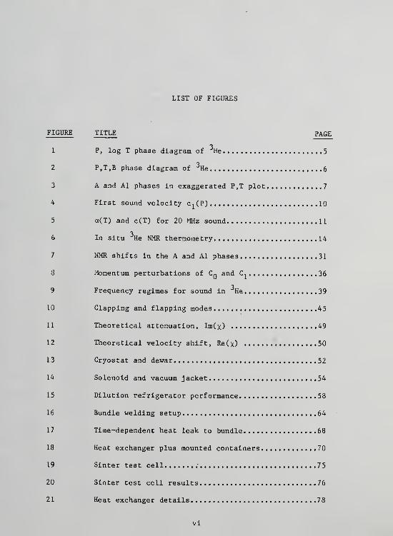
LIST OF FIGURES
FIGURE TITLE PAGE
1 P, log T phase diagram of3He 5
2 P,T,B phase diagram of 3He 6
3 A and Al phases in exaggerated P,T plot 7
4 First sound velocity c,(P) 10
5 a(T) and c(T) for 20 MHz sound 11
6 In situ He NMR thermometry 14
7 NMR shifts in the A and Al phases 31
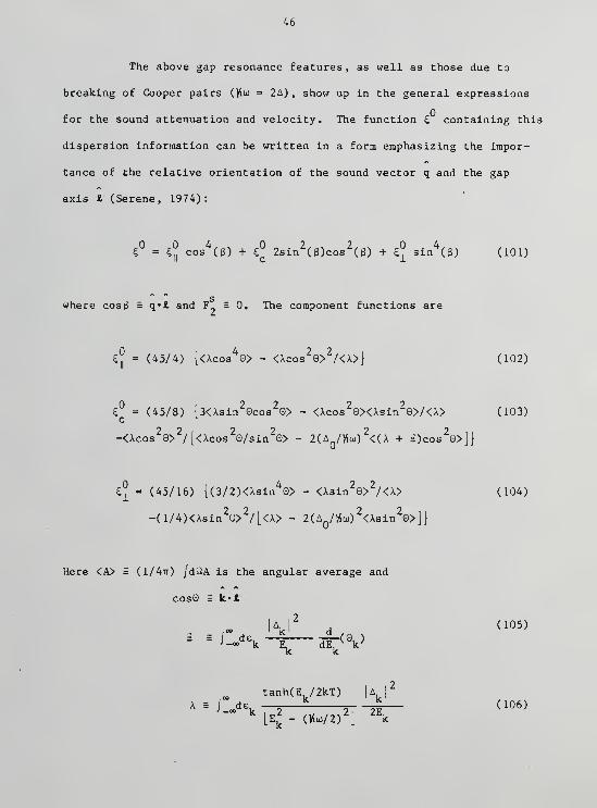
3 Momentum perturbations of C^ and C. 36
9 Frequency regimes for sound in He 39
10 Clapping and flapping modes 45
11 Theoretical attenuation, Im(x) 49
12 Theoretical velocity shift, Re(x) 50
13 Cryostat and dewar 52
14 Solenoid and vacuum j acket 54
15 Dilution refrigerator performance 58
16 Bundle welding setup 64
17 Time-dependent heat leak to bundle 68
18 Heat exchanger plus mounted containers 70
19 Sinter test cell ; 75
20 Sinter test cell results 76
21 Heat exchanger details 78
vi
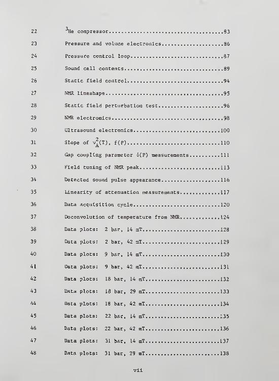
22 He conpressor 83
23 Pressure and volume electronics 86
24 Pressure control loop 87
25 Sound cell contents 89
26 Static field control 94
27 NMR lineshape 95
28 Static field perturbation test 96
29 NMR electronics 98
30 Ultrasound electronics 100
31 Slope of v*(T), f(P) 110
32 Gap coupling parameter 6(P) measurements Ill
33 Field tuning of NMR peak. 113
34 Detected sound pulse appearance 116
35 Linearity of attenuation measurements 117
36 Data acquisition cycle 120
37 Deconvolution of temperature from NMR 124
38 Data plots: 2 bar, 14 mT 128
39 Data plots: 2 bar, 42 mT 129
40 Data plots: 9 bar, 14 mT 130
41 Data plots: 9 bar, 42 mT 131
42 Data plots: 18 bar, 14 mT 132
43 Data plots: 18 bar, 29 mT 133
44 Data plots: 18 bar, 42 mT 134
45 Data plots: 22 bar, 14 mT 135
46 Data plots: 22 bar, 42 mT 136
47 Data plots: 31 bar, 14 mT 137
48 Data plots: 31 bar, 29 mT 138
vii

49 Data plots: 31 bar, 42 mT 139
50 Scaled attenuation maxima 142
51 Locations of attenuation maxima 143
52 Velocity shifts scaled to 9 bar 145
53 AB transition hysteresis 147
54 Phase-locked loop 153
Abstract of Dissertation Presented to the Graduate Schoolof the University of Florida in Partial Fulfillment of the
Requirements for the Degree of Doctor of Philosophy
DISPERSION OF 5 MHZ ZERO SOUNDIN SUPERFLUID 3He
NEAR T IN MAGNETIC FIELDSc
By
Robert Frank. Berg
December 1983
Chairman: Professor Gary G. IhasMajor Department: Department of Physics
Measurements of the attenuation and phase velocity changes
near T of 5 MHz ultrasound have been made in the A and Al superfluid
phases of3He at 2.05, 9.15, 18.18, 21.53, and 31.12 bar. All measure-
ments were performed in the low fields of either 14.3, 28.6, or 42
millitesla with the field direction parallel to the sound direction.
The finite field is important in four ways. First, it enabled the
anisotropic superfluid phases to be observed at arbitrarily low pres-
sures. Second, it caused a definite orientation of the order para-
meter £-vector with respect to the sound direction. Third, it allowed
observation of the narrow Al phase. And fourth, the exploitation of the
3He NMR shift in the superfluid gave precise, in situ thermometry for
the sound measurements. This is perhaps the first extensive use of
3superfluid He as its own thermometer.

The attenuation peak heights and the drops in the phase ve-
locity below T scale with pressure according to the predictions of the
collisionless theory for zero sound in the A-phase, while the absolute
attenuations observed are about one-quarter of that expected based on
this theory. The location of the attenuation maximum corresponds to the
expected clapping mode maximum at the lowest pressure but is signifi-
cantly colder than that predicted at all higher pressures.

SECTION 1
INTRODUCTION
Much of the progress made in man's general understanding of
the physical world has come about by conceptually separating the effects
peculiar to our immediate environment from the mora universal aspects of
nature. The force of friction is such a "particular" effect — realiza-
tion of this was necessary before a Newton could construct a valid set
of mechanical laws. Likewise, the fact that the vacuum is a more funda-
mental physical environment than a mixture of 80% nitrogen and 20%
oxygen at 1.01 bar pressure has spurred the unceasing development of
ever better vacuum pumps. Our usual environment, at a temperature of
about 300 K above absolute zero, can be interpreted as an ocean of
thermal excitations which affects all physical measurements made in
it. Many physical phenomena are very insensitive to room temperatures
but some of course are not. Indeed, many of nature's characteristics
are completely drowned out at 300 K and were only discovered when the
necessary low temperatures were reached. It is this ignorance of
nature's hidden beauties at low temperatures that has led physicists to
build ever better refrigerators.
The condensation of some form or another of matter has often
served as a milestone for low temperature physics. Examples are the
liquifaction of air (~80 K) in the latter part of the nineteenth century
and the liquifaction of helium (4.2 K) in 1908. If one generalizes the
1

concept of condensation to include ordering of any kind, then the exist-
ence of "superfluidity" can be viewed as a condensation in momentum
space. Such condensations of He atoms ("helium-II") and conduction
electrons ("superconductivity") were seen after the first liquifaction
of helium.
In general, a superfluid system contains constituent particles
(atoms or electrons) which are correlated over a distance much longer
than the average interparticle distance. This "connectedness" can cause
strange effects on a macroscopic scale, such as flow with absolutely
zero friction. Although some macroscopic effects of superfluids can be
tied together with a purely phenomenological theory (e.g. the London
equations for superconductivity) , a microscopic theory represents a
deeper understanding. A successful superfluid microscopic theory did
not exist until Bardeen, Cooper, and Schrieffer (BCS) (1957) and
Bogoliubov (1958) derived the now standard "BCS" pairing picture for
superconducting electrons. This theory of electrons in a metallic
lattice, based on the inherently quantum mechanical nature of fermions
,
soon caused speculation about superfluidity in other Fermi systems. The
chief such candidate was liquid He, the rare isotope of helium which
has a nuclear spin of 1/2, and the early 1960's saw theoretical predic-
tions of superfluidity in He (cf. Anderson and Morel, 1961; Balian and
Werthamer, 1963).
The actual critical temperature Tc
for the transition from the
normal to the superfluid state is not easy to calculate so it was not
until its (accidental) discovery in 1971 (Osheroff et al., 1972a) that
superfluid He made itself known in the laboratory. The decade of the
1970' s has seen an order of magnitude decrease in the routine minimum
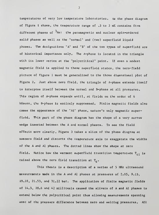
temperatures of very low temperature laboratories. As the phase diagram
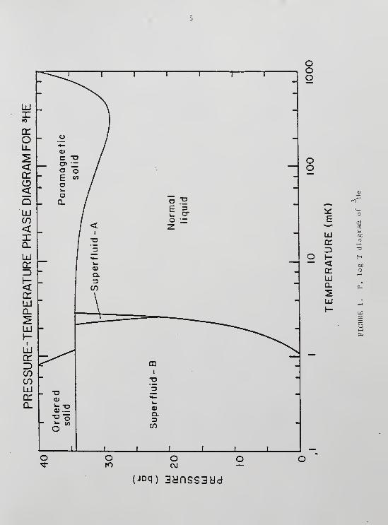
of Figure 1 shows, the temperature range of .3 to 3 mK contains five
3different phases of He: the paramagnetic and nuclear spin-ordered
solid phases as well as the "normal" and (two) superfluid liquid
phases. The designations "A" and "B" of the two types of superfluid are
of historical importance only. The A-phase is located in the triangle
with its lower vertex at the "polycritical" point. If even a modest
magnetic field is applied to these superfluid states, the zero-field
picture of Figure 1 must be generalized to the three dimensional plot of
Figure 2. Just above zero field, the triangle of A-phase extends itself
to interpose itself between the normal and B-phase at all pressures.
This region of A-phase expands until, at fields on the order of 6
kGauss , the B-phase is entirely suppressed. Finite magnetic fields also
cause the appearance of the "Al" phase, nature's only magnetic super-
fluid. This part of the phase diagram has the shape of a very narrow
wedge inserted between the A and normal phases. To see the field
effects more clearly, Figure 3 takes a slice of the phase diagram at
nonzero field and distorts the temperature axis to exaggerate the widths
of the A and Al phases. The dotted lines show the shape at zero
field. Notice how the warmest superfluid transition temperature T , is
raised above the zero field transition at T .
This thesis is a description of a series of 5 MHz ultrasound
measurements made in the A and Al phases at pressures of 2.05, 9.15,
18.18, 21.53, and 31.12 bar. The application of finite magnetic fields
of 14.3, 28.6 and 42 millitesla caused the slivers of A and Al phases to
extend below the polycritical point thus allowing measurements spanning
most of the pressure difference between zero and melting pressures. All

(joq) 3dnss3dd

^

I-
CD
(2
_J

8
of the measurements reported here were done at temperatures within 2% of
T since most of the important features of 5 MHz ultrasound dispersion
in the superfluid occur in this narrow range. Also, for temperatures
near T , the Ginzburg-Landau (e.g. see Landau and Lifshitz, 1969, ch.
14) theory which describes second-order phase transitions in terms of an
"order parameter" expansion is applicable, facilitating interpretation
of experimental results. The apparatus for this experiment were origi-
nally designed for an ultrasound investigation of single crystals of
3magnetically ordered solid He. Problems of heating and uncontrolled
solid growth redirected efforts to a liquid experiment for which the
apparatus were suited.
3Some of the earliest investigations of He used ultrasound at
5, 15, and 25 MHz (Paulson et al., 1973) and 10 MHz (Lawson et al.,
1973, 1974). The qualitative features observed in these and later
measurements are a sharp peak in the attenuation just below T accom-
panied by a small but swift decrease in the sound velocity. These
features are now understood to result from excitation of resonant modes
of the superfluid order parameter which, due to its complex tensor form,
has modes of a type unique in nature.
The propagation of sound in the superfluid phase should first
be placed in the perspective of sound propagation in the normal liquid
phase. The velocity of sound more than doubles as the pressure is
raised from zero to melting pressure (see Figure 4 constructed from data
tabulated by Wheatley, 1975). As the temperature is lowered the veloc-
ity and attenuation undergo changes connected with the finite lifetime
t of the normal liquid excitations ("quasiparticles") characteristic of
viscoelastic behavior (Rudnick, 1980). There is an attenuation peak

centered where the sound frequency is comparable to t (ujt~1) accompanied
by a small upward shift in the sound velocity, as shown in Figure 5 for
20 MHz sound at 29 bar (after Ketterson et al., 1975). The slopes on
the cold and warm sides of the attenuation peak are proportional to T
-2 3and T respectively. Sound propagation in He at frequencies and
(cold) temperatures such that cot>>1 is termed zero sound and represents
the propagation mode predicted by Landau (1957) on the basis of the
normal Fermi fluid kinetic equation in the collisionless limit. The
sharp changes in attenuation and velocity just below the superfluid
transition temperature T at~2.5 mK can be seen in Figure 5 also.
The effects of strong fields on the attenuation of A-phase
sound at multiples of 14.7 MHz at low pressure have been measured re-
cently in France (Avenel et al., 1981; Piche et al., 1982). These
measurements, chiefly concerned with nonlinear effects well below T,
find that the clapping resonance occurs at the predicted temperature at
low pressures, in agreement with the data reported here.
Using low fields to orient the superfluid, Ketterson et al
.
(1975) performed a series of 20 MHz ultrasound velocity and attenuation
measurements at pressures between 17 and 28 bar which has served as a
qualitative benchmark for my experiment. The measurements described
here also used an orienting field but this field was strong enough and
the temperature resolution fine enough to examine the A and Al phases
down to 2 bar.
The sound attenuation associated with the Al phase was studied
by Lawson et al. (1974) using fields up to 10 kGauss. They observed a
splitting of the characteristic superfluid attenuation peak which was
linear in the applied field. The Cornell group (Lawson et al., 1975)

10
S/tU)

11
2 9.3 bar
20.24 MHzafter Ketterson
et al. CI975)
2 5 10
TEMPERATURE CmK)
20
FIGURE 5. a(T) and c(T) for 20MHz sound
12
also has reported an observation of the velocity drop in the Al phase.
There are rapid drops at both T ^ and Tc2 . To my knowledge there is no
published theory explaining the dispersion of sound in the Al phase.
The choice of 5 MHz transducers represents a compromise. At
temperatures near T at 31 bar (~2.7 mK) , m~3 and the zero sound is not
quite fully "developed." Near T at 2 bar (~1.3 mK) , cjt~10 and the
propagation mode is essentially pure zero sound. Simply using higher
frequency transducers will insure pure zero sound at all pressures but
the energy of a sound quantum then becomes comparable to that of a
thermal fluctuation. For 5 MHz, JWk = 0.24 mK. Thus 5 and 10 MHz are
reasonable frequencies for zero sound transducers if one wishes
hw/kT «1.c
A few words should be mentioned about the techniques used for
3measuring sound attenuation, sound velocity, and He temperature. The
sound attenuation measurements were based on a conventional method: use
of a boxcar integrator to sample and average the transient signal in-
duced in a piezoelectric transducer by a short pulse of sound sent
across the sample cell. To measure phase velocity changes, the system
was configured as a phase-locked loop. This technique is less conven-
tional than the attenuation measurement and may even be unique to this
laboratory.
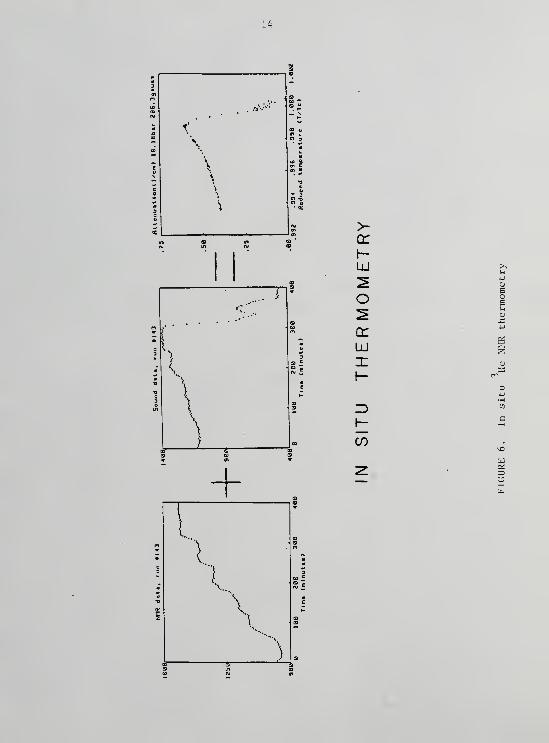
The discovery of large temperature-dependent nuclear magnetic
resonance (NMR) frequency shifts in the superfluid phase (Osheroff et
al. , 1972), besides stimulating much more experimental and theoretical
work in that area, also gave promise that the He sample -itself could be
used as a thermometer (e.g. see Richardson, 1977). To date this has not
been done, perhaps because of a lack of certainty about the necessary
13
calibration data. A few ancillary calibrations made in the course of
these experiments support the theoretical picture of the magnitidue of
these shifts (Leggett, 1974a) as well as corroborate most of the exist-
ing NMR shift calibrations. The net result is a basis for thermometry
in the A and Al phases accurate to ~10% but with a precision achieved in
magnetic fields of modest homogeneity which is comparable to LCMN ther-
mometry. The real advantage is a truly in situ thermometer, as Figure 6
illustrates. This shows the raw sound and NMR data on a run badly
disturbed by a time-dependent heat leak caused by a "touch" in one of
the cryostat vibration isolation mounts. After deconvolution , the sound
attenuation vs. temperature data fall on a curve similar to those of
"quiet" runs but with an inhomogeneous data point distribution along
that curve, where certain temperature regions were retraced due to heat
spikes followed by cooling.
The results of this series of measurements are given in the
last section chiefly in comparison against the collisionless theory of
sound dispersion in the superfluid A-phase. The amplitudes of the peak
attenuations and the velocity drops scale according to the predictions
of this theory, but at the higher pressures, the temperature locations
of the attenuation peaks are colder than predicted. A comparison with
theory using the numerical computation scheme of Wolfle and Koch (1978)
is probably required to see if a real discrepancy exists.
14

SECTION 2
PERTINENT THEORY OF 3He
2.1 General References
Current theoretical understanding of the superfluid phases of
3He rests on generalizations of the BCS theory of fennion pairing origi-
nally applied to metallic superconductivity (Bardeen, Cooper,
Schrieffer, 1957). Theoretical reviews of superfluid He have been
written by Leggett (1975), Anderson and Brinkman (1978), and Wolfle
(1979) and experimental reviews by Wheatley (1975, 1978) and Lee and
Richardson (1978). Shorter but more recent reviews can be found in the
proceedings of the 1981 "Low-Temperature-16" (Physica 107-110 , W.G.
Clark, ed.) and 1983 "Quantum Fluids and Solids" (AIP Conference Pro-
ceedings No. 103, E.D. Adams and G,G. Ihas , eds.) conferences. What
follows here is not intended as a review but only as a reminder of those
3theoretical aspects of He especially important for understanding the
experimental results presented in this dissertation. For purposes of
consistency, the notation will follow that of Wolfle 's review where
possible.
2.2 The Normal Fermi Liquid
Above the superfluid transition temperature of ~2 mK but
3significantly below the Fermi temperature of ~1 K, liquid He is well
described by Landau's "Fermi liquid" theory (Landau, 1956 and 1957).
The starting point for this theory is a gas of fermions of density n and
15

16
particle energies £, depending on momentum p=Hk and spin projection o.
At low temperatures this gas is nearly completely condensed into its
ground state: the Fermi sphere in momentum space of radius p p . The
Fermi energy £ and momentum p =|fik are related to the number density nr r r
by the following relations.
tf
2k2
ka 2m* U;
The quantity m* is an effective mass several times greater than the bare
atomic mass and is necessary for the connection to experimental
results. Similarly, the energies e, refer to excitations called quasi-
3particles, consisting of the collective motion of many He atoms but
still obeying the Paul! exclusion principle.
A consequence of the nearly condensed state of quasiparticles
is that the full three-dimensional momentum space picture can be reduced
to the two-dimensional one of excitations near the Fermi surface. Also,
the heat capacity and static magnetic susceptibility are then simply
proportional to the density of states near the Fermi surface.
This is possible because the quasiparticle distribution function is that
for fermions
a(e) = {exp[(e-u)/kT + if1
(3)
17
so that at low temperatures the distribution differs from a step func-
tion centered at the chemical potential u only in the neighborhood
3of u. Most properties of normal He can be described if one imagines
that the quasiparticles are coupled by a weak effective interaction so
that a deviation in the quasiparticle distribution from that of the
ground state changes the quasiparticle energy by
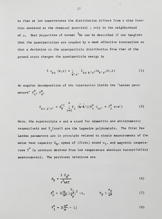
k.' a'
An angular decomposition of the interaction yields the "Landau para-
SF3
.meters" F , F .
fk k'o'
=Nf' ^
P*
Ci'i,)^ 6aa'
+ Fi
<" a,) (5)
Here, the superscripts s and a stand for symmetric and antisymmetric
respectively and P (cosO) are the Legendre polynomials. The first few
Landau parameters are in principle related to simple measurements of the
molar heat capacity CN , speed of (first) sound c^ and magnetic tempera-
ture T (a constant derived from low temperature absolute susceptibility
measurements). The pertinent relations are
3 <V>Np
- "£. (6)
irTcRT
C p
Mo* n V_ J' F m*
V '
r
F* = 3(?- lj (8)1 ^m '

18
F^=^f^-1 (9)
P F
The value of F can be obtained from spin diffusion measurements
(Leggett and Rice, 1968).
2.3 Superfluid Pairing
If the quasiparticle interaction is the least bit attractive,
at a sufficiently low temperature, the Fermi liquid picture must be
supplemented to account for the inevitable instability of quasiparticles
at the Fermi surface for forming bound pairs of opposite momenta.
Calculation of this critical temperature T from first principles is a
difficult problem but the pair interaction can be characterized in terms
of the Landau parameters. Doing so reveals that this interaction is
repulsive in the s-wave orbital angular momentum state (X=0) but attrac-
tive in the p-state (&=1). The repulsion in the s-state might be
3expected from knowledge of the hard-core repulsion between He atoms.
Pairing in the p-state, the basis of the most successful models of
3superfluid He, necessarily must, according to the Pauli exclusion
principle, be accompanied by a total spin S=l.
At the transition temperature, the quasiparticle energy spec-
trum is modified by the appearance of an energy gap and becomes
\-<\ + \<>1/2
<10)
where e, + e, is now the quasiparticle energy measured from the chemi-
cal potential (u = eF
at T=0) and A, is the off-diagonal mean field
acting on the Cooper pair (ko,-ka').

19
\ '=
\oo>=
IVkk'SkW (11)
k'
Equation (11) is mathematically analagous to equation (4) except that
now V^i., is the attractive interaction leading to the formation of pairs
and g, , ,is the probability amplitude of a Cooper pair (k'a,-k'a').
Here A, , is a complex 2x2 matrix in spin space. The actual magnitude
of the energy gap is given by
A,J = [(1/2) Tr (y£ } J
1/2d2)
At nonzero temperatures, the probability distribution in momentum space
for fermions leads to the particular form for the famous BCS self-
consistency "gap equation."
tanh (E, ,/2kT)
<W k \k' \<oo< 2-E- (13)
k' V
The gap equation uniquely defines the gap parameter for con-
ventional superconducting metals, where Ji=0. For £=1, though, several
3model states can be created. The fact that more than one superfluid He
state actually exists requires the careful consideration of the various
possible theoretical models. It is now widely, though not universally,
3believed that the two zero-field states of superfluid He are well
described by the so-called ABM and BW models. The ABM model (cf.
Anderson and Morel, 1961; Anderson and Brinkman, 1973) corresponds to
the experimental A-state and the BW model (cf. Balian and Werthamer,
1963) corresponds to the experimental B-state.

20
In order to discuss the various model states in detail it is
convenient to handle the three independent components of the 2x2 sym-
metric matrix A, , in the form of a vector d(k)
.
\aa'
~dl+ id
2 3
d + id.
(14)
The square of the energy gap can be written in terms of d(k) as
(A. A. ) ,= (d«d ) <5 , + i(dxd )«x , (15)
where x is the "vector" of Pauli spin matrices.
The d^'s, which deal with the spin part of the super fluid wave
function, specify the amplitudes of the gap parameter for those eigen-
states of the pair spin operator having eigenvalue zero. The connection
to the orbital part of the wave function is made by decomposing the d.'s
along the momentum axes.
d.(k) = V d. kJ a=l J
(16)
The 4*1, s=l model states of He are fully described by the tensor order
parameter d. .
2.4 Comparison of the ABM and BW States
Specification of a particular form for the complex
tensor d. leads to a state which can be compared with other model
states by means of their free energies described as expansions in the
order parameter. This Ginzburg-Landau expansion near T must involve
21
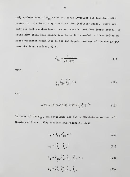
only combinations of d- awhich are gauge invariant and invariant with
respect to rotations in spin and position (orbital) space. There are
only six such combinations: one second-order and five fourth order. To
write down these free energy invariants it is useful to first define an
order parameter normalized to the rms angular average of the energy gap
over the Fermi surface, A(T).
d.J a
Ja V3 A(T)(17)
with
d. d. =1 (18)ja J J
and
+n i
1/2A(T) = [(l/4T;)/dii(l/2)Tr(AkA^)J
1/Z(19)
In terms of the d-a , the invariants are (using Einstein summation, cf.
Mermin and Stare, 1973; Brinkman and Anderson, 1973)
I = d. d. =1 (20)o ja ja K^ J
I1 l
d - d.|
2(21)
1 ' ja ja 1 v**^
I = d, d, d. d. a = 1 (22)2 ia ia j £ jB v ;
I. = d. d. d J . d., (23)
3 ia ja ig j3v '

22
I, = d. d. d. d.^ (24)4 ia jg ja iU
I_ = d* d* d. d. . (25)5 ia 13 ja jg
The free energy difference between the normal and superfluid states can
now be written as
F = F - Fs n
= - NF/2 (l-T/T
c)A
2(T) I
Q (26)
-2 45
+ (21/80)5(3)N_(irkT ) A*(T) l UF Ci-1
X ±
In the BCS weak coupling limit, the values of the g are
32
= 33
= 34
= -e5
= - 2 gi
= 1 (27)
A class of states discovered by Balian and Werthamer (1963)
minimizes the free energy for the weak coupling values in Equation
(26). The BW states are those unitary states given by
d. = A(T) ei<])
R. (28)ja ja
where $ is an arbitrary phase and R. is an arbitrary real orthogonal
(i.e. rotation) matrix. The BW state is the only l*Q state with an
isotropic energy gap.
|\(T)| = A(T) (29)

23
Since the BW state is the weak coupling minimum energy state,
the identification of the experimentally highly anisotropic A-state with
the ABM model state (Anderson and Brinkman, 1973) has thus been pur-
chased at the cost of abandoning the simple weak coupling picture of
-3
He, at least in those regions of the phase diagram where the A-state is
more stable than the B-state. Deferring this problem for a moment, the
ABM state can be characterized by the following unitary order parameter:
d = (3/2)i/2
A(T)d.(n +! ) (30)
where d is an arbitrary unit vector in spin space and n and n are arbi-
trary unit vectors in position space constrained only by n«« = .
These latter two vectors define the "angular momentum" vector by their
cross-product
I 2 nxm (31)
which lies along the axis of the anisotropic energy gap
1^(1)1 = (3/2)1/2
A(T)|sine
|(32)
where cost) = k*i.
2.5 Strong Coupling and the Finite Field Phase Diagram
The connection made by Anderson and Brinkman (1973) between
the experimental A-phase and the theoretical ABM model state used the
idea of "spin fluctuation feedback." As Leggett succinctly states, "the
basic physical idea of the Anderson-Brinkman theory is that the forma-

24
tion of the superfluid state modifies the pairing interaction between
quasiparticles , and that the precise nature of the modification depends
on the particular kind of superfluid state formed" (Leggett, 1975, p.
373). Spin fluctuation exchange, though perhaps the most important
feedback mechanism, is only one of several "strong coupling" effects
which might modify the pairing interaction. Quantitative spin-
fluctuation or "paramagnon" calculations have been performed by Brinkman
et al. (1974), Kuroda (1975), Tewordt et al. ( 1979a ,b), and Tewordt et
al. (1975, 1978). Instead of using the paramagnon approach, Rainer and
Serene (1976), Serene and Rainer (1979), and Sauls and Serene (1981)
have expanded the corrections to the 3. in powers of (kT /e ) and used
the "s-p" approximation for quasiparticle scattering for their calcula-
tions. Levin and Vails (1979) have combined both the paramagnon and s-p
scattering approaches. The net result of these various calculations is
a modification of the g from their weak coupling (kT /e * 0) BCS
values.
Comparison of the strong coupling calculations just mentioned
with experiment is obviously important but is complicated by the fact
that experimental measurements yield only combinations of the 3 . Even
though experiment contradicts the earlier predictions for some of the
6 combinations (Halperin et al., 1976), enough measurements to define
all five tf at any single pressure have not yet been performed, tost of
the useful measurements which can be performed toward this end exploit
the existence of the A, phase in a finite magnetic field. As shown by
Figure 3, the normal to A-phase transition is split by a magnetic field
into two transitions at I , and Tc2 . This splitting, a natural conse-
quence of the fact that He forms a spin-1 superfluid, can be viewed as
25
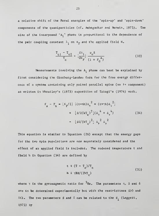
a relative shift of the Fermi energies of the "spin-up" and "spin-down"
components of the quasiparticles (cf. Ambegaokar and Mermin, 1973). The
size of the interposed "A," phase is proportional to the dependence of
the pair coupling constant X. on e„ and the applied field H.
T ,- T , dX u H
cl
T
c2- t^rJ -2— 03)
cd£
F (1 + FQ
a)
Measurements involving the A, phase can best be explained by
first considering the Ginzburg-Landau form for the free energy differ-
ence of a system containing only paired parallel spins (no t+ component)
as written in Wheatley's (1975) exposition of Takagi's (1974) work.
Fs
" Fn
=lV 2J t
(t- nh)\2+ C t+T*>A+
2}
+ [(V2(kTc
)
2j(A
f
4 + A+
4) (34)
- [65/(kTc
)
2J
Af
2A+
2
This equation is similar to Equation (26) except that the energy gaps
for the two spin populations are now separately considered and the
effect of an applied field is included. The reduced temperature t and
field h in Equation (34) are defined by
t = (T - T )/T° C
(35)h = YtfH/(2kT )
c
where y is the gyromagnetic ratio for He. The parameters n, 8 and 6
are to be determined experimentally but with the restrictions 3>0 and
6<1. The two parameters 3 and 6 can be related to the 8. (Leggett,
1975) by

26
3 = (7c(3)/16tt2)(3
2+ 3
4) (36)
-(3+3+23 )
6=(3
2+3
4)
(37)
where the value of the Rlemann zeta function is C(3) a 1 .202. Experi-
mental measurements of the characteristic BCS heat capacity jump at Tc
give information on the 3. • The three such independent measurements are
the following:
CA " C
N , 24 t 1
CN
TO my 32+3
4+3
5 27r23(1. 6)
CA1 " C
N r 24
CN
TO C(3)^ 2(32+3
4)
4lT2g
CB " C
N , 24 , 3
(38)
(39)
CN
" L 14 c(3) J 3(31+3
2)+(3
3+3
4+3
5)
'
(40)
Other experimental quantities yield additional information. There is a
small magnetic susceptibility increase in the ABM state of about 1%.
xA -xNn2(l+F*)
A M = 2 (41)XN
23(1+6) *;
The transition temperatures are given by
t = nh (42)
t = nh(1" 6)(43)C
2 (1+6)V
^
so that

27
2nh ,, , st l- t
2=Ti^) < 44 >
By defining an additional parameter to measure the substate with spin
projection zero, Equation (31) can be generalized to include the BW
state. Levin and Vails (1977) did this to obtain the transition temper-
ature between the A and B phases in a finite field below the polycriti-
cal point. Their rather complicated expression for t AR , which is
2proportional to h , will not be quoted here but it can be used to give
additional information on the 8. since the extra parameter characteriz-
ing the B-phase can be estimated by measuring the slope of the B-phase
susceptibility as a function of temperature.
Finally, the perpendicular NMR shifts in the A, -phase and A-
phase well below t2 give an independent measure of 6.
(dVL/dt)
Al 1-6
2L =V (45)
This will be discussed further in the next section.
2.6 NMR in the A and Al Phases
The magnetic characteristics of superfluid He differ dramati-
cally from those of the normal liquid. The susceptibility of the normal
liquid is an essentially temperature-independent constant equal to that
of a noninteracting Fermi system renormalized by the Fermi liquid para-
meter F,.
Y2*2
V4<N — (46)
1 + F

28
The nuclear magnetic resonant frequency to is simply proportional to the
magnetic field H, a la Larmour:
wL
= yH (47)
This picture changes below the superfluid transition at T ,
where the NMR A-phase resonance is seen to shift away from its normal
liquid value according to the relation
J = (yH)2+ U
2, £1* « (1 - T/T
c). (48)
Such a shift in the resonant frequency is possible only if non-spin-
conserving forces are invoked. In order to explain the A-phase fre-
quency shifts first seen by Osheroff et al. (1972), Leggett (1973,
1974a) modified the precession equations for the nuclear spins S by the
addition of a dipolar torque R^.
S=YSxH+R (49)
3The magnitude of the nuclear dipolar coupling between two adjacent He
atoms in the liquid is extremely weak. In temperature units it is
~10 K and could be readily neglected at typical experimental tempera-
tures , which are some 10 times higher, except for the correlations
intrinsic to the superfluid state. This causes the effective dipolar
coupling energy to be multiplied by the number of condensed Cooper pairs
in the system. The tendency for the pair wave function to seek its most
energetically favorable orientation is thus not "drowned out" by thermal
fluctuations.

29
For the ABM state, the equilibrium orientation caused by R^
aligns the d vector along the (orbital) angular momentum vector £. More
generally, on sufficiently short time scales typical of NMR experiments,
the motion of the d vector is given by
d = yd x (H - YS/x) (50)
Calculation of the dipolar torque Rq and the resulting shift
in the NMR frequency has been done for the various unitary phases of
superfluid He (Leggett, 1974a). In general the "longitudinal" fre-
quency (so called because of parallel-ringing magnetic resonance experi-
ments) is a product of a function of pressure f(P) and (1 - T/Tc).
a? = (2tt)2v2
= (2Tr)2f(P)(l - T/T ), T < T (51)
A A c c
where, for the ABM state,
f(P) = (tt/10)<R2>Y
2N (1 + F*)L*n(1.14 e /kT )]
2(kT )
2(AC/C
N) (52)
In Equation (52) e is an energy integral cutoff, estimated to be about
0.7 K by Leggett (1972). Most strong coupling effects are absorbed into
the experimentally measured ratio of the jump in the heat capacity at Tc
to the normal heat capacity (AC/C ). Here <R > is an angular average of
the square of the quasiparticle renormalization factor and is expected
to be on the order of unity. The quantity R^ which is averaged repre-
sents a modification to the spin current carried by particles of a free
gas to give that of the Fermi liquid (Leggett, 1965; Leggett and Rice,
1963).

30
IS.**.**- (53)m k. m
The nuclear magnetic resonance frequency also exhibits a shift
in the Al phase which can be easily understood in terms of the Ginzburg-
Landau equation (34). Takagi (1975) and Osheroff and Anderson (1974)
have discussed how the shift frequency v depends on temperature by
starting with the behavior of the two (different) order parameters for
the up and down-spin components for the liquid. It will be useful to
define a new temperature scale linear in T but with its zero at Tc 2
and
its "degree" equal to the width of the Al phase.
T - T
U 5 -Ci
- (54)
cl c2
Minimizing the free energy of Equation (34) results in the
following behavior of the gap magnitudes as a function of temperature.
A2
- A2
= , U < -1 (normal liquid) (55)+ T
A2= o , A
2= A(l + U) ,
-1 < U < (Al-phase) (56)+ T
A2
= BU, A2
= A + BU , < U (A-phase) (57)T T
Here, it is arbitrarily assumed that n >0, thus favoring an up-spin Al
phase. The constants A and B are related to the free energy parameters
3 and 6 by
A = (tj - t2)(kT
c)
2/6 (58)
B = A/(l - 6). (59)

31
3.0

32
A third constant C relates the perpendicular resonance shift to the
average of the two gaps
.
£- C[(A++ A
+)/2]
2(60)
The resulting shifts in the Al and A phases are then
n^ = (c/4)A(l = U) ,-1 < U < (61)
v. = (C/4)[A + 2BU + 2(A + BU) ' (BU) 'j , < U . (62)
A L
"Deep" into the A phase the shift can be well approximated by a linear
form
vf = (C/4)[2A + 4BU] , U > 1 (63)A L
The above theory gave an excellent fit to the NMR measurements
of Osheroff and Anderson (1974) done at the melting pressure in fields
of .49 and .74 Tesla. By taking the ratio of the slopes of the NMR
shift vs. temperature in the Al and "deep" A phases, they obtained a
value of o = 0.25 ± 5%. Figure 7 is a line drawing of this NMR shift
plotted in units of AC against the doubly reduced temperature U. The
particular slope ratio chosen for this drawing is 5.33 corresponding
to 6 = 0.25.
2.7 Sound Propagation in the Normal Fermi Liquid and the ABM-State
3One manifestation of the rich behavior of superfluid He due
to its complex tensor order parameter is in how the liquid disperses

33
sound. Many of the collective modes possible in the superfluid phases
can be directly excited by sound waves of the appropriate frequencies.
In order to give a qualitative explanation of sound experiments in the
A-phase I will, for the most part, quote the simpler calculations expos-
ited by Wolfle (1978) in his review on sound propagation in superfluid
3He.
At temperatures high enough or frequencies u low enough sound
propagation obeys the classical connections to compressibility k,
density p, and viscosity n. The velocity c, of such a hydrodynamic
mode, ordinary or "first" sound, is given by
c?
=7p- < 64 >
and the attenuation by
ai
= 7T- n * (65)3c^
The Fermi liquid compressibility is
2vP2d+F^)
(66)
;
_oindependent of temperature while the viscosity has a T temperature
dependence.
12-2n i. pvj « T (67)

34
3The velocity of first sound in He, taken from Wheatley (1975), is
plotted in Figure 4.
In general, transport properties such as viscosity can be
calculated only if one uses the general form of Landau's Fermi liquid
theory which includes the effects of quasiparticle collisions. For the
normal Fermi liquid, the mean quasiparticle lifetime between collisions
_2t is proportional to.T . The dynamic properties of the normal Fermi
liquid can be placed in a context which can be generalized to the super-
fluid phases by writing down the kinetic equation for the distribution
function of the quasiparticles. Starting with the Fermi distribution
for static thermal equilibrium
f? = [exp(£?/kT) + if1
(68)
the linear deviation cased by the perturbing (sound) field of wave
vector q and frequency (i), fif (r,t), can be written in terms of its
Fourier components
6fk(q,u) = Jd
3rdt[f
k(r,t) - f°]exp[i(fr - cot)
J (69)
The evolution of these Fourier components is governed by the kinetic
equation
Ku 5f, - e°5f, + fif, e° + f°fie, - fie, f° = -il. (fif) (70)k + k k- +k k- k.
This important equation uses the following notation: "0" indicates
equilibrium quantities, "±" means k±q, and fie is the change in the

35
quasiparticle energy caused by both the direct gain in the external
extfield 6e and the shift in the distribution function 6f , namely
The term on the right hand side of Equation (70) is the collision inte-
gral which operates on the deviation of the distribution function from
local equilibrium.
6fk
= 6fk " (l^) 6£
k < 72 >
What happens if the (sound) excitation period is much shorter
than the quasiparticle lifetime, i.e. ojt » 1? This is the "collision-
less" limit, equivalent to setting the dissipation term of Equation (70)
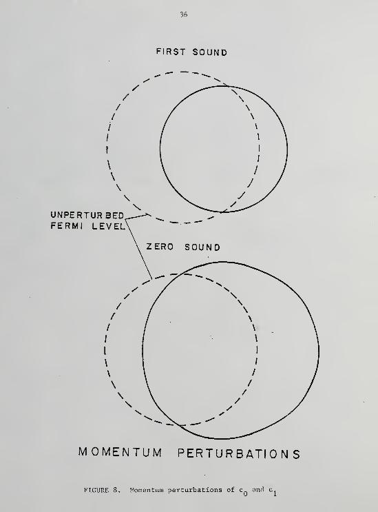
to zero. Landau (1957) showed that new propagation modes ("zero sound")
may then exist, corresponding to anisotropic oscillations of the Fermi
sphere (cf. Figure 8), with a separate mode for each i-coraponent of the
3quasi-particle interaction. He is such that there is only one propaga-
tion mode not strongly damped (longitudinal zero sound), corresponding
to a nearly spherical perturbation of the Fermi surface.
Equation (70) can be solved for its resonances by using the
conservation laws for the number and current densities 6n and j, which
are defined by
6n(q,o>) =I 6f (q,u) (73)ko '
j(q,«») =I (tfk/m)6f
k(q,u>). (74)
ko
36
FIRST SOUND
UNPERTURBEDFERMI LEVEL
MOMENTUM PERTURBATION S
FIGURE 8. Momentum perturbations of c and c

37
These conservation laws are the respective continuity equations
w6n = q-j (75)
wj I (k/m)(vFk-q)6f
k (76)ka
which are obtained from the kinetic equation by multiplying it by 1 or k
respectively and then summing over all k.
In the collisionless , zero-sound limit the velocity and atten-
uation are
c„ - c 2(1+4 F?> ? m*VF 9
-V-l TT—a il^^ •
(F250) (77)
C5(1 + O C
l
ao
=T5 l~
j
f ^) v '
3For He, the first and zero sound velocities differ by only~l%. This
gis so because the hard core repulsion leads to a large value of F
,
2especially at high pressure. The zero sound attentuation has a T
dependence, opposite that for first sound.
3The general dispersion relation for sound in normal liquid He
including the transition region u»T -^ 1 has been calculated by various
means (Rudnick, 1980; Wolfle, 1976b) and requires handling of the dissi-
pative term in Equation (70). Wolfle's approach is to construct an
approximate collision integral using the k-dependent quasiparticle
relaxation rates. His scheme allows generalization of the kinetic
equation to the superfluid states. Figure 5 from Wolfle (1973) includes
the result of such a normal fluid calculation fitted to the data of

38
Ketterson et al. (1975). The data points, which are well represented by
the theoretical fit, are not shown.
3The complicated nature of the superf luid He model states , as
compared to the Fermi liquid theory, can not allow a description of
superfluid sound propagation based solely on the scalar kinetic equation
(70). This was first verified experimentally (Lawson et al., 1973;
Paulson et al. , 1973) by the dramatic changes seen in the velocity and
attenuation of sound just below T for both the A and B phases. The
general features are a sharp peak in the attenuation with a width ~1% T
and a steep decrease in the velocity starting at T . There is also some
theoretical and experimental evidence for order parameter induced atten-
uation changes just above T (Emery, 1975, 1976; Paulson and Wheatley
1978; Samalam and Serene, 1978; Pal and Bhattacharyya , 1979). This
small effect will be neglected here.
3Simply by knowing the characteristic times of He, one might
estimate when changes in the sound dispersion will take place as the
frequency is varied. (Varying temperature changes the characteristic
times, also leading to dispersion.) Figure 9 shows the various regimes
defined by these (temperature-dependent) characteristic times, with
1/t dividing the hydrodynamic and collisionless regimes. The frequency
defined by the superfluid energy gap defines an additional region. For
a sufficiently warm temperature (T, on Figure 9), the gap frequency is
less than 1/x and the intervening regime can be called "gapless"; the
energy gap is not well defined due to quasiparticle collisions. At
colder temperatures (T2), the region above 1/x but well below A(T )/H is
called by Wolfle (1978) "macroscopic," signifying that the order para-
meter is in a local equilibrium state not significantly perturbed by the
sound frequency.

39
3
co

40
Calculations of the dispersion of pure zero sound (no quasi-
particle collisions) in the ABM state have been done by Wolfle (1973,
1975a, b, 1976a,b,c), Ebisawa and Maki (1974), and Serene (1974).
Wolfle's approach, originally due to Betbeder-Matibet and Nozieres
(1969), starts with the kinetic equation (70), drops the collision term,
and generalizes the distribution function to a matrix form appropriate
for a superfluid description. This results in expressions for the
perturbations of the order parameter which are induced by the sound
which in turn can be related to the expected sound dispersion.
Cooper pairing of quasiparticles of opposite momenta in the
superfluid state causes a new type of long range order in the system.
The quasiparticle (diagonal) distribution function
fkco'
(r'C) = /if i
3exp(lq.r)<a^ ^ > (79)
is then joined by an off-diagonal distribution proportional to the
expectation value of the pairing
*W (r ' C) = J^expUq-rKa^yy^ (80)
where a, (a^) is a creation (annihilation) operator acting on a state of
momentum k and k. = k ± q/2.
The quantity g^ is zero in the normal state and cannot even be
observed directly in the superfluid. Rather, changes in g, are seen by
their coupling' to f. . By defining a matrix distribution function in
particle-hole space

41
nk(r,t) =
and an analogous energy matrix
6k
1 - f-k
(81)
Vr.t) \
i -.
(82)
the linearized response to a sound wave (q,w) in the collisionless limit
can be written as the matrix analogue of Equation (70).
6nk - \+ 6n
k+ 6n
k V 6ek V + n
k+6ek
= ° (83)
~0The quantity 6n, = n, - n, is the linear deviation of the distribution
function from its equilibrium value, which is
°k=
2 L1 + W- tanh
^2kT^-k
(84)
As before, energies are measured from the Fermi surface
2e£ = k /2m* - u (85)
and the superfluid energy spectrum includes the effect of the energy gap
\ - C«J+ \0 1/2
(86)
The perturbations in the components of the energy matrix e.
are related to the perturbations of the two distribution functions.

42
6£k
=
^fkk'
6fk'
+6£kXt
(87)k'
6AkaC=
I gkak'o' 6gk'oa'
(88 >
k'
In analogy to the normal Fermi liquid equation (4), the equilibrium
energy gap is related to the off-diagonal distribution function by the
self consistency equation
\oo' "l,
gkak'a ,gk'aa' (89)
thus defining gkak , a,.
The matrix kinetic equation (83) is a system of linear inte-
gral equations which can be solved for the case where the interactions
^kk' anc* ^kk' are assume d to be independent of the magnitude of
k (|k| = k ). Wolfle's (1976b) approach is to rewrite Equation (83) byr
defining "vectors" composed of combinations of 6f , , 6g, , 6e, , and 6
A
and multiply them by appropriate matrices which contain only equilibrium
quantities for their entries. Solving the resulting matrix equation is
then more straightforward, leading to explicit expressions
for 6e and 6Zl.
6ek - 6e
k
xt= Vf f
kk. fer^-Ki - ^,)«v -Y ^6£
k«+ 6£-k .J
,(hu + h
2n') . ,,, A
+ . ..+—2 Xk'
(6Ak'
Ak« " V 6V (90)
4|\.
6\ +l gkk. k'
6\- T^^^yK- C« + *»')«v
(91)

43
For the above two equations, the following abbreviations were used:
n E tfVq/m* (92)
k= (l/2E
k ) tanh(Ek/2kT) (93)
,2 r-d£
k , 2 2d\,
^(l.-.T) -= -Al^l2
ioo_
L (^)2Qk+ n
2
£k_] (94)
Dk
E (hoo)2[(hu))
2- 4E^j - n
2L(hoo)
2- 4e
2]
(95)
Equations (90) and (91) were arrived at assuming that the gap
parameter A . is unitary but otherwise are not specific to any modelaa'
state. Specialization to the ABM state requires the particular form of
the ABM gap, namely Equation (30) inserted into Equation (14).
A^, = i/372 A(T)[<m + ii.kJLd.(TT2
)aa ,j (96)
Now, by a particular choice of coordinates, the perturbation of the gap
parameter can be written in terms of the azimuthal components of the
first spherical harmonic Y,„
.
r im
+1 3
6A, = i/6^ l-^J
172Y, (k) 6d .(t.tJ , (97)
Icoa' hw L, .
L,
v2
J lm ml j 2 aa'm=-l j=l
Using these forms for the gap and its perturbation induced by the sound
in the general equations (90) and (91) results in an expression for each
of the three expansion parameters 6d , 6d n , Sd .. Collective modes
(resonant oscillatory distortions) of the order parameter show up as
poles of the 6d in the complex frequency plane.

44
The equilibrium (no sound) order parameter is proportional to
Y, , (k) as can be seen by choosing coordinates such that n = x
and = y in Equation (96). It turns out that there is no pole asso-
ciated with 6d .
There is one pole associated with 6d ; excitation of this
mode amounts to a distortion of the equilibrium gap parameter by an
amount proportional to Y« (k). In the limit of T near Tc , the temper-
ature dependence of this mode's frequency is (Wolfle, 1975)
hu = [(4/5)(2/6 - 3)]1/2
/37T A(T)LV " /v /J 'N '
(98)
= 1.2326 AQ(T)
where A (T) = /3/2 A(T) is the maximum magnitude of the ABM gap.
The 6d mode is often referred to as the "clapping" mode as the
Yi_i (k) oscillations results in a movement of the n and m vectors
towards and away from each other as Figure 10 shows.
The equation for 6d yields two modes . These modes are some-
times called "normal flapping" and "super flapping." Figure 10 illu-
strates normal flapping: n and m "flap" up and down, thus rocking
the Ji-vector back and forth away from its equilibrium position. Near
T , the temperature dependences of the two flapping frequencies are
given by
H»nfl= A75 A
Q(T) [l - (28/3tt
4) ;(3)(A
Q(T)/kT
c)] (99)
*Usfl= 2 V T)
I-1 " (
28/ 5ir4 >5< 3><VT)/kTc) ] U00)

45
4
"CLAPPING"
"FLAPPING"
FIGURE 10. Clapping and flapping modes
46
The above gap resonance features , as well as those due to
breaking of Cooper pairs (Kw = 2A) , show up in the general expressions
for the sound attenuation and velocity. The function E, containing this
dispersion information can be written in a form emphasizing the impor-
tance of the relative orientation of the sound vector q and the gap
axis I (Serene, 1974)
:
E? = 5° cos4(B) + E? 2sin
2(g)cos
2(B) + i°. sin
4(0) (101)
II c l
where costf = q«t and F = 0. The component functions are
5° = (45/4) {<Xcos4Q> - <Xcos
2Q>
2/<X>} (102)
5° = (45/8) {3<Xsin20cos
20> - <Xcos
20><Xsin
20>/<X> (103)
c
-<Xcos20>
2/[<Xcos
20/sin
20> - 2(A /Jtu>)
2<(X + £)cos
20>]}
5° = (45/16) {(3/2)<Xsin40> - <Xsin
20>
2/<X> (104)
-(l/4)<Xsin20>
2/[<X> - 2(A /Ha))
2<Xsin
20>]}
Here <A> = (1/4tt) JdiiA is the angular average and
cos0 = k»i
l\|2
d(105)
'k E. dE,_x
k'
tanh(E /2kT) \\|
2
x ~= J'-«dek 7-2—^ 27 "2I7- ( 106)k
E2
- (tfw/2)2 2\

47
For T near T„
,
X = ii LjfjJtanh^j
2 -2-T7T + (g-) (107)[(JW2A ) - sin 0J c
For zero sound of low enough frequency, X simplifies to (Kui/kT) times a
function of (A /yico) only. This makes it possible to express the sound
attenuation and velocity in terms of a universal function defined by
X = (2kT/5KWK° (108)
The sound attenuation is then
tf2
a E2 im(x) (109)
coFokT
and the shift in the sound velocity from its zero sound value Cq is
tl^l |^Re(x) (HO)°0 F^kT
Figures 11 and 12 from Wolfle (1978) show what the imaginary
and real parts of the components of the universal function x(An /Vi<jj) look
like. Although pairbreaking at A /ftw = 1/2 is implicitly included, the
dominant features are the various gap resonance modes. In particular,
X shows a strong, sharp peak in the attenuation with a corresponding
feature in the velocity shift. The overall anisotropy of dispersion is
of course due to the anisotropy of the order parameter itself. The
maximum value of the attenuation for any orienation is proportional to
the prefactor of Equation (109).

48
a « —= (111)max s
0c
So far, the effects of quasiparticle collisions have been
ignored. A good accounting of their effects, which should include the
2background T attenuation behavior and a broadening of the collective
modes peaks, might start by adding a dissipative term to the right hand
side of the matrix kinetic equation (83). This is a generalization of
the scalar collision integral. Wolfle and Koch (1977) were able to
construct an approximate form of this dissipative term that was numeri-
cally tractable. Their calculations, involving some 30 double integrals
on angle and energy, give fair agreement with the attenuation data of
Paulson et al. (1977) and the attenuation and velocity data of Ketterson
et al. (1975). In particular, the clapping attenuation peak is broaden-
ed and the corresponding "derivative-like" structure in the velocity
shift is no longer present.
The presentation of the preceding pages , chiefly concerned
3with the theory of collisionless sound in superfluid He, is intended to
serve as a basis for comparing the experimental results to be described
later in this thesis. In our experiment the magnetic field was parallel
to the sound vector, thus orienting the Ji-vector of the superfluid
perpendicularly to the sound (except for a small fraction next to the
container boundaries). Thus only x, of Equations (101) through (111)
will be considered for comparing the sound attenuation and velocity
data.

49
lm{x}Scaled attenuation
i\u« kTT=Tr
CA^TVhaO2a |-T/T
FIGURE 11. Theoretical attenuation, Im(x)

50
2.0 1.0
(A (TJ/hu>)2
cc l-T/Tc
FIGURE 12. Theoretical velocity shift, Re(x)

SECTION 3
APPARATUS
The apparatus for performing these experiments necessarily
include the refrigerator, constructed before my tenure at the University
of Florida. Since construction details have not been reported previous-
ly, I will do so here. Much of the general discussion of refrigeration
principles follows Lounasaaa (1974).
3.1 Large-Scale Features
The cryostat and most electronic systems rest in a 24 m
copper screen room. Electronic filtering for the 125 VAC lines in-
cludes, besides the usual low pass network, provision for elimination of
the occasional bursts at 3510 Hz used for campus clock synchroniza-
tion. All vacuum pumps and the dilution refrigerator gas handling board
are outside the screen room as well as the computer and signal averager
for data acquisition. The signal averager has analog electrical connec-
tions to the screen room electronics via three 1-MHz low-pass filters.
Figure 13 indicates the gross dimensions of the cryostat and
dewar. The "super-insulated" dewar (Cryogenics Associates, 62 liters)
and cryostat are suspended from a triangular aluminum plate which is
supported at its three corners by optical-bench air mounts. For demag-
netization of copper nuclei, a custom-built, American Magnetics,
niobium-titanium superconducting 8 tesla magnet is used. This magnet,
with its compensating coils, is mounted directly on the 10-liter vacuum
51
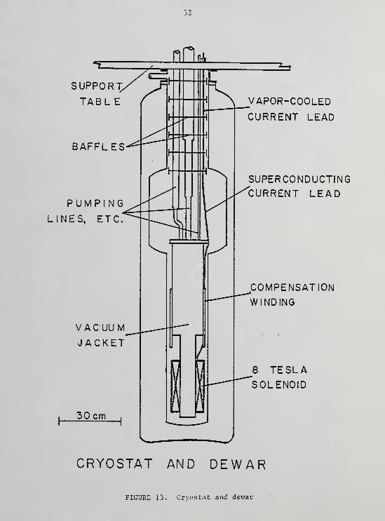
52
SUPPORTTABL E
BAFFLES
PUMPINGLINES, ETC.'
VACUUMJACKET
30 cm
nJZk
VAPOR-COOLED
CURRENT LEAD
SUPERCONDUCTINGCURRENT LEAD
COMPENSATIONWINDING
8 TESLASOLENOID
CRYOSTAT AND DEWAR
FIGURE 13. Cryostat and dewar

Figure 14
8 Tesla superconducting solenoid and some of the contents of the
vacuum jacket.
A 1 K pot
B still
C continuous concentric heat exchanger
D discrete heat exchangers
E mixing chamber
F flexible heat link
G squeeze connection to bundle flange
H copper demagnetization bundle
I thermal shields
J vacuum jacket wall
K indium heat switch
L vertical Helmholtz coil pair
M compensation windings
N 8 tesla solenoid

54
SOLENOID AND VACUUM JACKET
FIGURE 14. Solenoid and vacuum jacket
55
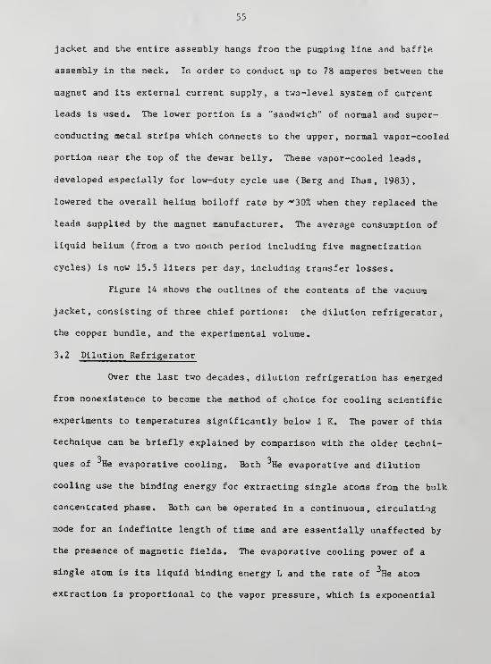
jacket and the entire assembly hangs from the pumping line and baffle
assembly in the neck. In order to conduct up to 78 amperes between the
magnet and its external current supply, a two-level system of current
leads is used. The lower portion is a "sandwich" of normal and super-
conducting metal strips which connects to the upper, normal vapor-cooled
portion near the top of the dewar belly. These vapor-cooled leads,
developed especially for low-duty cycle use (Berg and Ihas , 1983),
lowered the overall helium boiloff rate by '"30% when they replaced the
leads supplied by the magnet manufacturer. The average consumption of
liquid helium (from a two month period including five magnetization
cycles) is now 15.5 liters per day, including transfer losses.
Figure 14 shows the outlines of the contents of the vacuum
jacket, consisting of three chief portions: the dilution refrigerator,
the copper bundle, and the experimental volume.
3.2 Dilution Refrigerator
Over the last two decades, dilution refrigeration has emerged
from nonexistence to become the method of choice for cooling scientific
experiments to temperatures significantly below 1 K. The power of this
technique can be briefly explained by comparison with the older techni-
3 3ques of He evaporative cooling. Both He evaporative and dilution
cooling use the binding energy for extracting single atoms from the bulk
concentrated phase. Both can be operated in a continuous, circulating
mode for an indefinite length of time and are essentially unaffected by
the presence of magnetic fields. The evaporative cooling power of a
single atom is its liquid binding energy L and the rate of He atom
extraction is proportional to the vapor pressure, which is exponential

56
in temperature. Thus, the overall cooling power goes as
Q(evaporation) *• L exp(- ?-=) (112)kT-
and in practice the highest possible pumping speeds give a minimum
3temperature of about 0.3 K for a pure He cryostat,
Dilution refrigeration works because of the nonzero solubility
of "*He in He at arbitrarily low temperatures, about 6.4% below 40 raK.
Cooling, obtained by transfering He atoms from the pure into the dilute
phase in a "mixing chamber," is driven by an osmotic gradient, which in
turn is produced by pumping He vapor from a "still" which is at a
temperature high enough to give a reasonable circulation rate. Even
3 2though the cooling power per He atom decreases with temperature as T ,
the circulation rate, n, is independent of mixing chamber temperature so
that the overall power for dilution cooling is
. . 2Q(dilution) - n T . (113)
If careful account is taken of factors such as thermal isolation and
viscous heating, the practical limit of a dilution refrigerator is
determined by the quality of the heat exchangers between the incoming
and outgoing liquid streams. Within the past few years, temperatures
below 3 mK have been achieved by groups using fine silver powder heat
exchangers (e.g. Frossati, 1978; Oda et al., 1983).
Our dilution refrigerator is of conventional (pre-1978) de-
o 3sign. The 1 K pot, of 270 cm volume, liquifies the incoming He. A
"pickup" capillary, with an impedance dictated by the heat load on the

57
4pot, replenishes the He supply from the 4.2 K bath. A manually oper-
ated valve allows the pot to be filled in about 10 minutes at the time
of first cooldown or if the pickup impedance becomes blocked. Such
blocking did occur during this quite extended experiment and daily use
of the manual fill valve was required. Careful use of the valve re-
sulted in negligible entropy increase of the experiment, even during the
1 mK runs
.
3 3The He still (100 cm ) contains a "film burner" designed for
a He purifier (Kirk and Adams, 1974) and reduces the He content of the
vapor removed to about 1%.
The heat exchanger system between the still and the mixing
chamber consists of a continuous exchanger followed by six step ex-
changers. The continuous exchanger, 1.5 m in length, is simply a thin-
walled copper-nickel tube of 1 .8 mm inside diameter which contains the
dilute stream and an inner capillary of 0.51 mm inside diameter for the
concentrated stream. Each of the six step exchangers is a pair of
copper tubes silver-soldered together and packed with copper powder
(-200 mesh, C-110, U.S. Bronze). Bulk flow is through a central longi-
tudinal tube created by a "greened" steel wire during the sintering at
3 3900° C. The volume available to the helium ranges from 2 cm to 4 cm in
each of the six exchangers.
The 30 cm copper mixing chamber contains copper powder (-400
mesh) sintered in place at 850°C.
Figure 15 characterizes the performance of our dilution refri-
gerator by plotting its cooling power as function of mixing chamber
temperature for three different circulation rates. The circulation
rates of 17, 25, and 36 micromoles per second correspond to still heater

o
o
<
cr

59
powers of 130, 360, and 700 microwatts respectively. Film burner power
was 140 microwatts for each curve. The minimum mixing chamber tempera-
ture in the unloaded state is about 14 mK although temperatures as low
as 10 mK lasting for a few hours have been observed. These latter inci-
dents have always been associated with the lowering of the magnetic
field at the experiment or the copper bundle and are attributed to
demagnetization of the copper nuclei in the mixing chamber by the fring-
ing fields of these magnets. This effect is verified by the comparable
heating seen at the mixing chamber when one of these fields is raised at
the same speed used when mixing chamber cooling was observed.
3.3 Nuclear Cooling Stage
Achieving refrigeration sufficient to study the superfluid
phases or the magnetically ordered solid phase of 3He usually requires
adiabatic nuclear demagnetization cooling. Although cooling to these
temperatures is possible with Pomeranchuk compression or demagnetization
of the electronic paramagnetic salt cerous magnesium nitrate (CMN), the
former is limited to melting curve pressure (34.3 bar at 3 mK) and both
lose cooling power just below the ordering temperatures of the refriger-
ants, about 1 mK for both 3He and CMN.
Nuclear cooling can be simply understood by considering the
thermodynamics of a noninteracting nuclear dipole system placed in a
magnetic field, B. The Zeeman interaction energy for each dipole is
£m
= -ugmB (114)
where m is the magnetic quantum number, g is the nuclear gyromagnetic
ratio, and u = e!ii/2Mc is the nuclear magneton. For n moles, the
partition function is

60
I „ nNUgmB
Here I is the nuclear spin and N is Avogadro's number. The expressions
for entropy and magnetization derived from Z can be simplified by ex-
panding in the parameter uglB/kT. If the effect of the dipolar field is
included, the entropy, S, magnetic susceptibility, x» and heat capacity,
Cg, can be written as
2 2
S = nR to (21+1) -A (B +
\)
(116)
2u To
X=4 (117)
JUBW)_
whereR = ideal gas constant
\i free space permeability
2 2A = N 1(1+1) u y g /3k = molar nuclear Curie constant
o o
2b dipolar interaction
Under ideal conditions of no heat leaks or nonnuclear heat capacities,
the final temperature, T^, after reducing the field from B^ to B^, is
related to the initial temperature by
Bf
2 +b2 1/2
T _ f T (119)f
Bi2+ b
2 1
and the heat capacity is unchanged.

61
CB(T
f) = CgCT^ (120)
The construction of the nuclear cooling stage for our cryostat
is similar to that described by Muething (1979). The two major differ-
ences between the Ohio State Univeristy nuclear stage and ours at the
3University of Florida are the wire diameter and the He heat exchanger;
these differences will be discussed in more detail. As was done at OSU,
copper was chosen for the demagnetization material. Copper gives the
advantages of high thermal conductivity, no superconducting transition,
ready availability in wire form, and low cost. Its disadvantages are
-12its low Curie constant (A = 4.04x10 K/mole) and its relatively large
Korringa constant of 1.1 sec # K.
3.4 Bundle Construction
Since the construction details of our bundle differ somewhat
from those of the Ohio State University bundle, the building process
will be described here. The gross features of the final product are a
close-packed cylindrical copper wire bundle 5.6 cm in diameter and 40 cm
long welded to an 11 cm diameter copper plate or flange. This flange
3 ^has an array of holes for clamping devices, such as the He heat ex-
changer, to the bundle.
The wire chosen for the bundle was a commerical grade, coated
magnet wire (Essex Corporation) whose special, high temperature insula-
tion (Allex) allowed the bundle to withstand temperatures of 300° C for
extended periods of time. Thus, the wires were protected during the
welding operation and the slight flowing of the Allex during annealing
could be used to bond the bundle together without the use of epoxy,

62
suspected as the cause of large time dependent leaks (Konter et al .
,
1977). The wire chosen was (#24 AWG, 0.51 mm diameter) based on the
measured 4.2 K resistivity of the wire material, p = 5x10 ohm*m. The
net eddy current heating power in a changing magnetic field, B, is
p - safes?s2
(no
where N is the number of wires of length I and radius r. For a typical
"cold" rate of 3xl0~ Tesla/sec this gives P = 10 nW, an acceptable
level for this process.
Preparation of the wire for bundle construction commenced by
winding some 200 turns onto a 27 cm diameter light aluminum drum. Two
cuts through the wires along the axis of the drum gave two tresses of
wires 42 cm long. About forty such tresses were made. Allex is resist-
ant to most chemical stripping agents so, in order to remove 4 cm of
insulation from one end of each tress, the tresses were dipped in a bath
of molten sodium hydroxide (NaOH) contained in a stainless steel
beaker. Immediately afterwards, the wires were bathed in a weak solu-
tion of acetic acid to neutralize any residue of the strong base.
Finally, they were rinsed twice with distilled water in an ultrasonic
cleaner.
Collecting the wires together for welding was begun by
straightening the tresses and carefully laying them together in a
trough. A hose clamp then drew the bare ends into a close-packed array
5.1 cm in diameter. A 5.1 cm i.d., 5.6 cm o.d. cylindrical OPHC copper
collar with an interior bevel on one end was forced around the wires by
alternately pounding on the collar and sliding the hose clamp down

63
towards the center of the wires. The protruding 3 ran of base wire
provided the fill metal during welding. The bundle of wires was immedi-
ately clamped into a support jig, designed so that most of the bundle
could be lowered into a glass nitrogen dewar (see Figure 16). The dewar
was filled with liquid nitrogen until only the OFHC collar and the
stripped ends were not immersed. Then the tops of the wires and collar
were housed in a glove box continuously purged by helium gas drawn from
evaporating liquid helium. An arc welder operating at five kilowatts in
the D.C. mode with an argon gas shielded tip fused the wire tops to-
gether. After correcting minor nonuniformities of this first weld by
filing, the bundle flange, an 11 cm diameter plate with a central hole
to mate to the bundle, was slid over the fused wire tops and came to
rest on the collar. The two pieces were then welded together using the
glove box and other procedures as before, after which the entire as-
sembly was ready for wrapping.
The bundle flange was now fitted with a bearing race so that,
by inserting the bearing balls, the flange with its protruding wires was
left free to turn with respect to this support. The next step was to
attach two #24 Allex insulated copper wires at the top of the bundle,
which, as it rotated, would be wrapped along its length by these
wires. The two wires were fed from opposite sides by a spring and brake
assembly, which used feedback to give a very constant and balanced
tension. As the wrap progressed, the bundle was struck sharply and
simultaneously with two hammers in an opposing fashion all around the
perimeter of the bundle. This compressed the wires of the bundle to-
gether so that, when the wires were eventually cut and tied off, the
final diameter was < 5.6 cm and quite uniform.

64
Q-
LlI
in
LU
UJ-J
Qz:
3GD

65
The wrapped bundle and flange structure was removed from the
rotating support and inserted into a clamp designed to straighten the
bundle and preserve its alignment with respect to the flange. Heating
for five days at 275°C in a slightly flowing He atmosphere annealed the
copper and caused the Allex insulation to flow slightly and thus bond
the individual wires together. It was possible to avoid completely
using epoxy and still have a quite rigid structure.
The last step was to trim the bundle to the appropriate length
using a "glass wheel" (as used for cutting stainless steel tubing). The
cut end showed only a few dislocations in the hexagonal close-packed
array of 9000 wires.
3.5 Thermal Isolation and Heat Leaks
Effort expended on refrigeration for a millikelvin cryostat
must be complemented with measures to prevent the flow of heat into or
generation of heat within the final cooling stage. All material connec-
tions between stages of different temperatures were constructed to
minimize undesired heat flow along these connections. The load bearing
supports between stages are 1 cm diameter AGOT graphite rods. All
electrical connections and helium carrying capillaries were heat sunk at
the 1 K pot, the still, the mixing chamber, and the copper bundle.
Electrical heat sinks usually relied on a thin layer of cigarette paper
soaked with Stycast 2850FT (Emerson and Cuming) as an electrically
insulating thermal conductor. Capillaries were thermally anchored by
soldering 10 to 30 cm of the line around a metal post and bolting the
post to the refrigerator. Silver solder was used at the lower stages to
avoid problems with soft solder superconductivity. The lowest tempera-
ture capillary connections were made with 300 micron (12 mil) o.d.

66
copper-nickel tubes. Most electrical connections were made with copper-
nickel wire except for the connections to the lowest temperature stage,
which were made with Nb-Ti superconducting wires (the copper cladding
was removed from all but the end connections of each length of wire).
Two nested thermal shields anchored at the still and mixing
chamber reduce the influx of heat due to blackbody radiation. The upper
portion of these shields is of welded sheet copper and the lower "tail"
section is a cylinder of longitudinally aligned copper wires ("coil
foil") coated with a hardened slurry of epoxy (Stycast 1266, Emerson and
Cuming) and finely ground coconut charcoal. This design (Tanner et al.,
1977) has a high infrared absorption coefficient while minimizing the
heat load due to eddy current heating during changes of the copper
bundle field. The bottoms of the shields are aligned with each other,
the vacuum jacket, and the copper bundle by a series of teflon "bicycle
wheels" with nylon mono-filament spokes. The influx of infrared radia-
tion to the lower temperature stages was also reduced by placing tabs of
copper foil at the vacuum jacket pumping port and over unused feed-
through holes at the various refrigerator stages.
The heat link between the bundle and the mixing chamber con-
sists of the heat switch, the flexible link, and the squeeze connec-
tors. The squeeze connectors allow quick mounting and removal of the
bundle from the cryostat, thus allowing the mounting of the experiment
to be chiefly a table-top procedure. To establish the squeeze connec-
tion, a gold-plated copper collar, welded to the flexible link, is
pressed over a matching gold-plated copper post welded to the bundle
flange. A thick nylon ring is then pressed around this assembly. As
the cryostat cools, contraction of this nylon ring provides the strong

67
squeezing force necessary (Muething et al. , 1977). The flexible link is
2two bundles of copper wires each about 1 cm in cross section. At its
upper termination is a heat switch of conventional design which consists
of two copper posts of semicircular cross section separated by Vespel
(DuPont) rods and surrounded by a small persistable superconducting
solenoid. The superconducting link is a strip of indium about 1 cm long
and about 10 ram in cross-section (March and Symko , 1965). Indium is
readily available in pure form, is easily fabricated and attached to the
refrigerator by virtue of its low melting point, and has a relatively
low critical field of 28 millitesla.
Despite these various thermal isolation measures , the heat
leak to the bundle was frustratingly high at 50 to 100 nanowatts for the
first several weeks of the run during which the data for this thesis
were taken. Tests showed that no nearby electrical equipment and, with
the possible exception of the dilution refrigerator mechanical pump, no
nearby mechanical equipment were implicated. The heat leak due to
electrical and capillary connections to the bundle was expected to be
< 1 nanowatt. As the data on Figure 17 show, the heat leak to the
bundle eventually dropped to about 3 nanowatts or about 50 picowatts per
mole of refrigerant. Since we knew of no changes external to the cryo-
stat which could have caused this drop in the heat leak, we surmised
that the depletion of some energy reservoir in the bundle had been
taking place during this time (see Pobell, 1982).
Our primary suspect for the time-dependent heat leak is ortho-
para conversion of hydrogen molecules. The associated energy, transi-
tion rate, and equilibrium concentrations of this process are well known
for the bulk solid (Silvera, 1980). Such a heat leak as a function of
time would be

68
500-
0-P CONVERSIONOF 3.5 I0" 4 MOLE H2
20 5 100 200 500 1000 2000 5000TIME AFTER COOLDOWN (HOURS)
HEAT LEAK TO BUNDLE
FIGURE 17. Time-dependent heat leak to bundle

69
Q = 3.8xlO~3
n(122)
(Kt+l/X(0)JZ
where t is the time in hours of cooldown from 300 K. (essentially infi-
nite temperature as far as the ortho concentration is concerned) to "0
K" and n is the number of moles of hydrogen involved. In the denomina-
tor X(0) is the high-temperature limit of ortho concentration (3/4) and
K is the rate constant (0.019 hour" ). The curve plotted onto the data
of Figure 17 is Equation (122) for 3.5xl0~ mole of hydrogen. Ignoring
the residual heat leak of about 3 nanowatts, the fit is rather good.
_3About 5x10 mole of hydrogen gas was used as an exchange gas for cool-
ing the cryostat down to 10 K and, although it should have ended up in
solid form at the bottom end of the vacuum jacket wall, we cannot be
certain of this. Also, a recent report by (Mueller et al., 1983) cites
the discovery of pockets of hydrogen gas in copper used for construction
of a refrigerator. Without some form of microscopic analysis to prove
otherwise, such a possibility for the bundle wires or the body of the
3He heat exchanger is only speculative.
3.6 Superfluid-Handllng Apparatus
At the heart of the cryostat is the experimental region out-
lined schematically by Figure 18. The "anchor" to the bundle flange is
3the He heat exchanger and on this structure the compressor, strain
gauge, and cell body sit. Demountable struts raise the body of the heat
exchanger to center the cell body in the magnetic field. These two OFHC
copper pieces bolt to both the bundle flange and the heat exchanger; the
mating surfaces are gold-plated. Also bolted to the bundle flange are a
carbon resistance thermometer, a resistance heater, a heat sink for the
70
HEAT/EXCHANGER SOUND
'CELL BODY
LIQUID 3HE CONTAINERS
FIGURE 18. Heat exchanger plus mounted containers
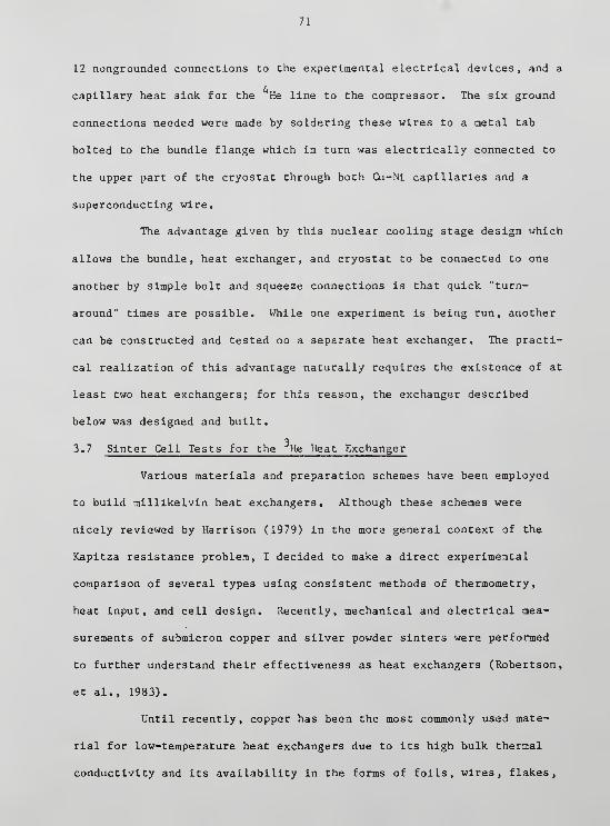
71
12 nongrounded connections to the experimental electrical devices, and a
capillary heat sink for the He line to the compressor. The six ground
connections needed were made by soldering these wires to a metal tab
bolted to the bundle flange which in turn was electrically connected to
the upper part of the cryostat through both Cu-Ni capillaries and a
superconducting wire.
The advantage given by this nuclear cooling stage design which
allows the bundle, heat exchanger, and cryostat to be connected to one
another by simple bolt and squeeze connections is that quick "turn-
around" times are possible. While one experiment is being run, another
can be constructed and tested on a separate heat exchanger. The practi-
cal realization of this advantage naturally requires the existence of at
least two heat exchangers; for this reason, the exchanger described
below was designed and built.
3.7 Sinter Cell Tests for the He Heat Exchanger
Various materials and preparation schemes have been employed
to build millikelvin heat exchangers. Although these schemes were
nicely reviewed by Harrison (1979) in the more general context of the
Kapitza resistance problem, I decided to make a direct experimental
comparison of several types using consistent methods of thermometry,
heat input, and cell design. Recently, mechanical and electrical mea-
surements of submicron copper and silver powder sinters were performed
to further understand their effectiveness as heat exchangers (Robertson,
et al., 1983).
Until recently, copper has been the most commonly used mate-
rial for low-temperature heat exchangers due to its high bulk thermal
conductivity and its availability in the forms of foils, wires, flakes,

72
and powders. The copper powder we used (Vacuum Metallurgical) in these
tests was nominally 0.03 micron in particle diameter. However, electron
micrographs showed a characteristic diameter closer to 0.07 micron. The
black appearance of this powder is apparently due to the presence of a
large (60-80%) copper oxide volume fraction. This estimate is based on
the 16% mass loss that occurred upon heating a sample to 450°C in a
hydrogen atmosphere.
In order to build an oxide-free copper exchanger, we tried two
approaches. The first was to reduce the powder at low temperatures
until a 15% mass loss was achieved. The resulting powder, which had
suffered a little particle size increase (.08 to .14 micron diameters)
was then "cold-pressed" (at room temperature) into a copper cell. The
second approach was to first press the raw powder into the cell and then
heat it in a reducing atmosphere to obtain a 15% mass loss. A third
approach, untried by us, is to "presinter" the powder before pressing it
into the cell for sintering. The "presintering" might more appropri-
ately be called "oxide reduction."
In recent years, due to its low nuclear heat capacity and
relative cleanliness, silver powder, especially the .07 micron "Japanese
powder", (Vacuum Metallurgical) has been the most popular material for
millikelvin heat exchangers. Since a sample of our silver powder suf-
fered less than 1% mass loss upon heating to 300°C, we decided to cold-
press the raw powder into a silver-plated copper cell with jio_ heat
treatment whatsoever.
Palladium, with its high paramagnetism, showed promise as a
heat exchanger material for He samples , as verified by foil measure-
ments of Avenel et al. (1973). However, to our knowledge, only two

73
palladium powder exchangers have ever been built. Our palladium test
cell was sintered according to the recipe devised at Ohio State
University, (see Muething, 1979) which employs carbon monoxide and
hydrogen as reducing agents, and helium to flush out the hydrogen before
cooldown to prevent its absorption by the palladium.
A total of five cells, whose particulars are described in
Table 1, were built. A cross-section of a sinter test cell is shown in
Figure 19. The chamber in the oxygen-free copper body was cut out by
spark, etching and abrasive cleaning was necessary to remove the result-
ing residue on the walls. Final cleaning consisted of an acid bath dip
and heating in a hydrogen atmosphere to remove surface oxides.
For economical thermometry, 0.5 watt, 220 onm "old" Speer
carbon resistors were ground to a 1.6 mm thickness and attached to leads
with silver paint. These thermometers, calibrated against the He
melting curve, worked well down to 5 mK when immersed directly in the
3liquid He.
Thermal time constants of the sinter cells were measured by
applying a current pulse to the Cu-Ni heater sufficient to cause an
initial 5 to 10% temperature rise over the outside temperature, which
was that of the temperature-regulated mixing chamber. After the passage
of a small signal transient, attributed to the response of the thermo-
meter bridge electronics to the heater pulse and the finite response
3time of the carbon thermometer, the He temperature decayed approxi-
mately exponentially to that of the mixing chamber. The thermal time
constants obtained were converted to thermal boundary resistances using
the interpolated and extrapolated heat capacity data of Greywall and
Busch (1982). For comparison purposes, these resistances are plotted
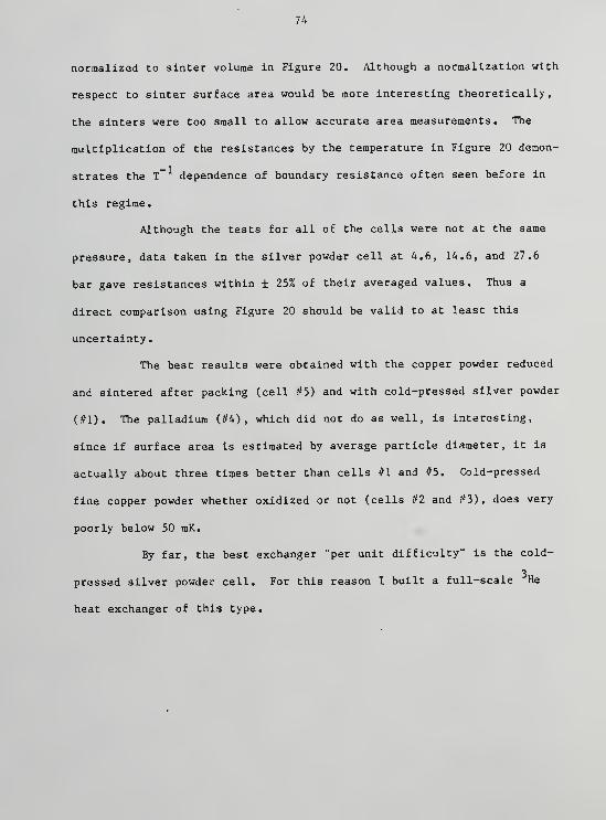
74
normalized to sinter volume in Figure 20. Although a normalization with
respect to sinter surface area would be more interesting theoretically,
the sinters were too small to allow accurate area measurements. The
multiplication of the resistances by the temperature in Figure 20 demon-
strates the T dependence of boundary resistance often seen before in
this regime.
Although the tests for all of the cells were not at the same
pressure, data taken in the silver powder cell at 4.6, 14.6, and 27.6
bar gave resistances within ± 25% of their averaged values. Thus a
direct comparison using Figure 20 should be valid to at least this
uncertainty.
The best results were obtained with the copper powder reduced
and sintered after packing (cell #5) and with cold-pressed silver powder
(#1). The palladium (#4), which did not do as well, is interesting,
since if surface area is estimated by average particle diameter, it is
actually about three times better than cells #1 and #5. Cold-pressed
fine copper powder whether oxidized or not (cells #2 and #3), does very
poorly below 50 mK.
By far, the best exchanger "per unit difficulty" is the cold-
3pressed silver powder cell. For this reason I built a full-scale He
heat exchanger of this type.

75
X

76
CO
COUJcr
COUJ
crLUh-
CO

77
Table 1; Descriptions of sinter test cells
#1. 0.07 micron Ag powder (Vacuum Metallurgical) cold-pressed at 850
3bar into Ag-plated cell. 43% packing fraction. 4.6 bar He pres-
sure.
#2 0.03 micron Cu powder (Vacuum Metallurgical) was first reduced
(165-180°C in He+H2atmosphere for 120 minutes; this caused 15.3%
mass loss) then cold-pressed at 1110 bar. 43% packing fraction.
314.6 bar He pressure.
#3 Untreated 0.03 micron Cu powder (Vacuum Metallurgical) cold-pressed
3at 1200 bar. 34% packing fraction. 14.6 bar He pressure.
#4 1 micron Pd powder (Leico) packed at 1110 bar then sintered accord-
ing to OSU recipe (Muething, 1979) using CO (810-860°C for 2 hours)
and H2
(570-600° C for 5 hours) and He "flushouts" while cooling.
352% packing fraction. 3.2 bar He pressure.
#5 0.03 micron Cu powder (Vacuum Metallurgical) packed at 855 bar then
sintered at 200-220°C for 230 minutes in H2atmosphere. This
caused 13% axial shrinkage and 15.5% mass loss. 34% packing frac-
3tion. 3.2 bar He pressure.
33.8 He Heat Exchanger Construction and Performance
The gross dimensions of the OFHC copper body of the heat
exchanger and the locations of the cell mounting holes (see Figure 21)
were chosen to duplicate those of the first exchanger for this cryostat,
which used sintered palladium powder. Three independent wells, each
divided into two or three annular sections by 0.8 mm thick cylindrical
copper walls, were cut into the copper body using a spark etch milling

s
111II
^
1IIIHI
ts
1 111i
EXCHANGER BODY CROSS-SECTION
3 cm
HEAT EXCHANGER TOP FACE
FIGURE 21. Heat exchanger details

79
machine (EDM). The dividing walls insured that no portion of the sinter
would be more than 1.6 mm from bulk copper. For sealing vessels to the
heat exchanger wells with gold o-rings , a sealing surface much harder
than annealed copper is required. To this end, and also to provide hard
material for tapping the bolt circles for cell attachment, six flat
brass rings were inlaid into grooves cut into the exchanger body at the
upper and lower entrances of the three wells. The best means of doing
this turned out to be first coating the appropriate exchanger and brass
ring surfaces separately with silver solder (Silvaloy 355, Eutectic)
,
removing all traces of flux, and finally brazing the rings into place in
a hydrogen atmosphere at 700° C using greened stainless steel weights to
prevent "floating" of the rings. This final brazing simultaneously
annealed the copper body. A final, light EDM cut was made to align the
inside diameters of the brass inlays with that of their respective
wells. The protuding inlays were then machined to nearly the level of
the copper body and drilled and tapped with appropriate bolt circles
(#2-56).
At this stage leak tests uncovered two passages between screw
holes tapped into the brass inlays and their respective wells due to
gaps in the solder apparently caused by flux residue. These were suc-
cessfully sealed by injections of Stycast 2850FT (Emerson and Cuming).
Preparation of the exchanger for packing with silver powder
including light scrubbing to remove the EDM residue, followed by an acid
bath dip to remove a partial brass surface on the copper body caused by
diffusion of zinc from the brass inlays during annealing. All surfaces
of the heat exchanger body were then plated with silver using a commer-
cial jeweler's electroplating solution and fine silver anode (Jadow).

80
Although the depth of the wells probably attenuated the electric field
near the well bottoms , this was apparently compensated by the electro-
negativity difference of silver and copper and the end result was at
least an optically thick coating of silver on all exchanger surfaces.
After silver plating, the brass sealing surfaces were lapped
to the same level as the copper body and then polished by wet sanding
with fine emery paper. Final cleaning was done in an ultrasonic bath.
Packing the annular sections of the exchanger wells was done
in layers one to three mm thick per pressing in order to assure uni-
formity of volume packing fraction throughout. The nominally 0.07
micron diameter "Japanese" silver powder was packed using a press con-
structed from an inexpensive 1.5 ton automobile hydraulic jack. Pres-
sures applied to the silver varied from 370 to 410 bar. The final
pressing left the 487 gram copper exchanger body holding some 61 grams
of pressed silver powder. The volume packing fraction of the three
wells varied from 46% to 48%.
Figure 21 shows the arangement of the two sizes of holes which
were drilled into the packed sinter. The two large holes, 2.4 mm in
diameter, anticipate possible future use of the exchanger in flow exper-
iments and greatly enhance hydrodynamic heat flow through the helium
between the top and bottom of each well. The array of small holes, 1.0
mm in diameter, decreases the average distance between bulk liquid
helium and the sinter interior.
Addition of the array of small holes improved the thermal time
constant of the He exchanger at 3 mK from about 30 to about 6
minutes. The required density of these holes should be comparable to
*the characteristic length of the sinter, I , defined by (see Muething,
1979)

where
*
<**> 2 =TT I (123)
h = Kapitza conductance per unit areaK.
k
k k,* 3 s
k„+k3 s
3k_T = He conductance in the sinter
V,A = sinter volume, area.
Using hK derived from a measurement of Ahonen et al. (1978) and k found
by normalizing the bulk value by the sinter to bulk ratio for palladium
found by Muething and setting V/A to that of a single spherical particle
*of 0.07 micron diameter gives I - 2 mm.
3While the final version of this cold-pressed silver powder He
heat exchanger has not been completely characterized as a function of
helium temperature and pressure its performance has been entirely satis-
factory. Below 10 mK, the thermal time constant for heat flow between
1/2 mole of helium and the copper bundle is about six minutes except at
temperatures much below three millikelvin where the x of the copper
nuclei becomes the important thermal "resistance" (x T is 1.1 sec*K for
copper)
.
3.9 Compressor
Only two of the three heat exchanger wells were used in this
3experiment. Most of the liquid He sample was contained in these two
wells and in the compressor. This compressor, whose outline is shown by

82
3Figure 22, allows the He pressure to be precisely controlled, espe-
3cially at pressures above 29.3 bar, where solid He begins to form in
the warmer regions of the sample fill line.
This arrangement of concentric bellows is not the usual one
3for He compressors. The more common figuration is that used in
3Pomeranchuk (1950) compressors where the He bellows is everted so that
3a compression consists of an expansion of the He bellows, thus avoiding
inadvertent compression of the solid helium which might form in the
bellows' folds. Since solid growth in the compressor was not desired in
the first place, the present design saves valuable space in the experi-
mental region.
The two bellows are made of single-ply beryllium copper
(Robert Shaw). The top and bottom beryllium-copper pieces act as caps
3for the He container walls of 321 stainless steel. The post inside the
3 3He bellows acts as a stop and conserves He volume while still provid-
3ing channels sufficient for keeping the He in thermal equilibrium with
the rest of the sample. All metal-to-metal seals were made with Stycast
2850FT (Emerson and Cuming) to avoid the use of superconducting solder;
these seals held to pressures of at least 37 and 17 bar on the
3 4He and He sides respectively. Movement of the bellows could be de-
tected by measuring the capacitance between electrodes glued to the
outside of the He brass cap and the inside of the stainless wall.
The position of this compressor determines the total experi-
3mental He volume. The maximum stroke of 8.6 mm causes a volume change
of 1.0 cm . Thus, when the He volume in the compressor is increased
3 3from its minimum of 7.6 cm to its maximum of 11.0 cm , the total exper-
3 3 3imental He volume decreases from 11.4 cm to 10.4 cm .
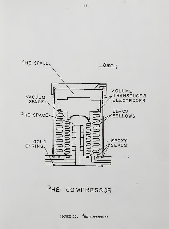
83
4 HE SPACE
VACUUMSPACE
3 HE SPACE
GOLDO-RING
mm
VOLUMETRANSDUCERELECTRODES
BE-CUBELLOWS
EPOXYSEALS
HE COMPRESSOR
FIGURE 22. He compressor

84
As mentioned in the introduction, attempts to grow single
3crystals of solid He in the sound transducer region failed because of
solid nucleation elsewhere. My chief suspicion is that this solid grew
inside the compressor due to a heat leak associated with "fast"
(~1 bar/hour) compression. Irreproducibility and minor nonmonotonic
behavior of the volume transducer signal suggests that the outer elec-
trode may have become partially unglued from the stainless steel.
Friction due to this defective transducer or to "scraping" of other
parts may be the source of trouble. As part of a pressure regulation
loop there have been no problems with the compressor, however.
3. 10 Pressure Measurement and Control
A capacitive strain gauge measured the sample pressure in
3situ. The design used is similar to the original one first used for He
by Straty and Adams (1969). Figure 23 shows a schematic diagram of the
electronics used for the pressure and volume measurements. Although
both transducers required a three-terminal capacity measurement, a total
of only five cryostat wires was used by putting both signals on a common
line at different frequencies. In both systems, a ratio transformer
primary is driven at the reference frequency of either one or five
kilohertz. The secondary is then adjusted so that the voltage at the
sum point is nulled. The reference capacitors (20 pF) are anchored to
Lthe 1 K He pot.
Submicron position changes could be seen by the volume trans-
ducer but it had non-monotonic and irreproducible behavior attributed to
a loose electrode. The sensitivity of the pressure transducer was about
10 bar and worked well up to 36 bar. The settings of the ratio trans-
former for the strain gauge were related to sample pressure through a

85
calibration made against a 1500 psi (103 bar) Heise Bourdon pressure
gauge. 22 points between 4 and 36 bar were recorded. This procedure
took several hours as each point required usually more than 10 minutes
to change the pressure and wait for pressure equilibrium. The resulting
data were fit to a second-order polynomial with an rms deviation of less
than 0.1 bar which is more than the estimated inaccuracy of the Heise
3gauge obtained from He melting curve comparisons at the nuclear order-
ing temperature (1.0 mK) and at the melting curve minimum pressure (318
mK).
The pressure measurement system described above was used to
control the sample pressure by the feedback scheme outlined in Figure
324. The error signal of the He pressure lock-in amplifier drives a
heater in a He "bomb" suspended just beneath, and weakly coupled ther-
mally to, the top of the vacuum jacket. By appropriately fine tuning
the He and He amounts the bomb can be caused to operate near the
liquid-vapor critical point at 5.2 K where the expansivity of the
4He is large. Gross adjustments to the sample volume and density are
4 3made by adding or removing gas through the He and He fill capillar-
ies. The two control valves are always left shut except during these
adjustments.
The dependence of sound velocity on pressure imposes a re-
quirement on the stability of the pressure during a single run where
changes in phase velocity are measured. Referring to Figure 4 shows
-5 -4that a velocity precision of Ac/c '~10 requires AP'^-'IO bar in the
region where (dc/dP)/c is greatest. The stability of pressure regula-
tion, as estimated by observation of the volume transducer output,
indicated that this requirement was met.

86
CO
o
oLU_JL±J
LU
CE

PRESSURE
TRANSDUCER
ELECTRONICS
HE HE
PRESSURE CONTROL LOOP
FIGURE 24. Pressure control loop

3.11 Sound Cell Contents
The cylindrical beryllium-copper cell slung underneath the
3middle well of the He heat exchanger contains an assembly of parts
3bathed in He and shown by Figure 25. Nine separate pieces fit inside
the outer sleeve machined from Stycast 1266 (Emerson and Cuming). This
sleeve is a hollow cylinder with four longitudinal slots allowing good
3He thermal conduction and absolute alignment of the radiofrequency (RF)
coils with respect to externally applied fields.
3The fraction of the total He sample actually probed is only
about 1%: that portion contained between the two sound transducers
separated by the cylindrical spacer. Sound pulses are transmitted and
received by the two 9.53 mm diameter, 5 MHz, gold-plated X-cut quartz
piezoelectric transducers. Ground connections to the transducers' inner
faces are made via silver paint coating the ends of the spacer. Elec-
trical connections to the opposite faces of the transducers are made by
light, nonmagnetic springs, which also hold the transducers in place
against the spacer. A small amount of indium solder holds a connecting
wire (not shown) to the end of each spring.
The machined epoxy spacer defines the sound path length (6.25
± .05 mm) and diameter (5.0 mm). These estimates allow for the thermal
ocontraction of Stycast 1266 (Swift and Packard, 1979). Some 23 mm of
radial holes, including those created by the "crenelations" at the
spacer ends, provide thermal conduction paths for the helium inside.
In order to perform NMR measurements on the same sample probed
by the sound, a flattened "saddle-shaped" RF coil was wound on grooves
cut into the spacer. The location of this coil is the reason that the
more usual choice of metal or quartz for a spacer material was not

CO
LU\-
-z.
oo
LU
CJ
Q~Z.
Z>
OCO

90
made. The coil was constructed by winding half of some 100 to 150 turns
of #44 (45 micron) formvar-insulated copper wire on each side of the
"saddle". At 930 kHz, its inductance was 95 microhenries and its Q was
15. The coil's orientation placed the field it produced perpendicular
to the plane of rotation of the static field.
One interesting note is that a naive calculation of the eddy
current heating induced in the gold transducer coating can give a value
as high as many nanowatts at the RF levels and frequencies routinely
used in this experiment. Apparently the details of the RF field config-
uration and its intersection with the gold film prevent such a disaster
from occurring. The heating seen at RF currents ten times that ordi-
narily used was less than or on the order of one nanowatt.
Not shown in Figure 25 is a miniature heater for nucleation of
3solid growth for magnetically ordered solid He experiments. This
3heater consisted of a dab (~0.1 mm ) of Stycast 1266 (Emerson and
Cuming) containing 0.07 micron silver powder (Vacuum Metallurgical) near
the percolation limit. This slurry was hardened across the cut faces of
a twisted pair of 45 micron formar-insulated copper wires. Heaters of
this type had resistances of several hundred to several thousand ohms
which were stable at low temperatures. Their small size enabled the
3location of nucleated solid He to be well controlled. Unfortunately,
unpredictable "burnouts" limited their reliability. For the purposes of
this (liquid) experiment it is sufficient to know that the unused heater
extends radially inward to the cell center in the midplane of the spacer
and takes up only 2% of the sound path area.
A second RF coil consisting of 220 turns of #44 (45 micron)
formvar-insulated copper wire was wound in a "double solenoid" config-
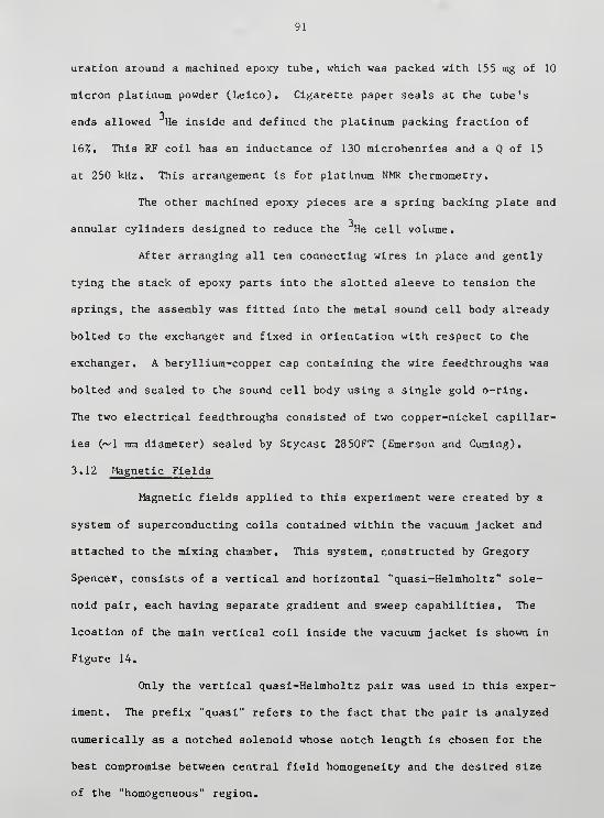
91
uration around a machined epoxy tube , which was packed with 155 rag of 10
micron platinum powder (Leico). Cigarette paper seals at the tube's
3ends allowed He inside and defined the platinum packing fraction of
16%. This RF coil has an inductance of 130 microhenries and a Q of 15
at 250 kHz. This arrangement is for platinum NMR thermometry.
The other machined epoxy pieces are a spring backing plate and
3annular cylinders designed to reduce the He cell volume.
After arranging all ten connecting wires in place and gently
tying the stack of epoxy parts into the slotted sleeve to tension the
springs, the assembly was fitted into the metal sound cell body already
bolted to the exchanger and fixed in orientation with respect to the
exchanger. A beryllium-copper cap containing the wire feedthroughs was
bolted and sealed to the sound cell body using a single gold o-ring.
The two electrical feedthroughs consisted of two copper-nickel capillar-
ies (~1 mm diameter) sealed by Stycast 2850FT (Emerson and Cuming).
3.12 Magnetic Fields
Magnetic fields applied to this experiment were created by a
system of superconducting coils contained within the vacuum jacket and
attached to the mixing chamber. This system, constructed by Gregory
Spencer, consists of a vertical and horizontal "quasi-Helmholtz" sole-
noid pair, each having separate gradient and sweep capabilities. The
lcoation of the main vertical coil inside the vacuum jacket is shown in
Figure 14.
Only the vertical quasi-Helmholtz pair was used in this exper-
iment. The prefix "quasi" refers to the fact that the pair is analyzed
numerically as a notched solenoid whose notch length is chosen for the
best compromise between central field homogeneity and the desired size
of the "homogeneous" region.
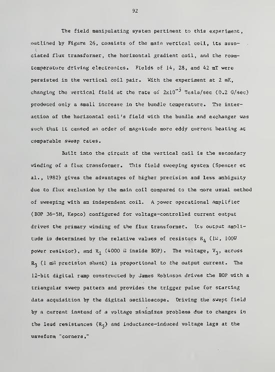
92
The field manipulating system pertinent to this experiment,
outlined by Figure 26, consists of the main vertical coil, its asso-
ciated flux transformer, the horizontal gradient coil, and the room-
temperature driving electronics. Fields of 14, 28, and 42 mT were
persisted in the vertical coil pair. With the experiment at 2 mK,
changing the vertical field at the rate of 2x10 Tesla/sec (0.2 G/sec)
produced only a small increase in the bundle temperature. The inter-
action of the horizontal coil's field with the bundle and exchanger was
such that it caused an order of magnitude more eddy current heating at
comparable sweep rates.
Built into the circuit of the vertical coil is the secondary
winding of a flux transformer. This field sweeping system (Spencer et
al., 1982) gives the advantages of higher precision and less ambiguity
due to flux exclusion by the main coil compared to the more usual method
of sweeping with an independent coil. A power operational amplifier
(BOP 36-5M, Kepco) configured for voltage-controlled current output
drives the primary winding of the flux transformer. Its output ampli-
tude is determined by the relative values of resistors R/, (lii, 100W
power resistor), and Ri (4000 Q inside BOP). The voltage, V^ , across
R- (1 mft precision shunt) is proportional to the output current. The
12-bit digital ramp constructed by James Robinson drives the BOP with a
triangular sweep pattern and provides the trigger pulse for starting
data acquisition by the digital oscilloscope. Driving the swept field
by a current instead of a voltage minimizes problems due to changes in
the lead resistances (Re) and inductance-induced voltage lags at the
waveform "corners."

93
Figure 27 indicates the field homogeneity over the sample seen
3 -5by the He NMR coil. The sweep of 4.1x10 Tesla superposed on a steady
14.3 raT shows that the majority of the affected He is in a field of
-4homogeneity AB/B = 4x10
The horizontal gradient coil was used to enhance the tip of
the NMR peak. Its effect on the overall field homogeneity or central
field value was not important.
Field perturbations caused by the bundle demagnetization
solenoid and large steel objects outside the cryostat caused some minor
problems. In spite of its compensation winding, the bundle solenoid
contributed a field to the sample region amounting to some 0.02% of the
solenoid central field. Thus, even small demagnetizations produced a
measurable shift of the NMR resonance. In addition, the bundle solenoid
exhibited a relaxation of its fringing field comparable to the magnitude
of the shift with a characteristic time of one hour after small (~3 mT)
demagnetizations
.
A drift of ~lxl0 Tesla/sec superposed on most NMR measure-
ments was attributed to decay of either the persisted Helmholtz pair or
bundle solenoid, equivalent to magnet decay times of order 10 or 0.1
years respectively.
A number of spontaneous jumps in the observed NMR frequency
—9corresponding to field changes of ~10 Tesla were eventually attri-
buted to changes in the static field caused by changes in the positions
of nearby large steel objects such as gas bottles or nitrogen dewars.
Figure 28 shows the effect produced by various positions of a 0.1 m
hollow steel dewar. The observed field shift has very little hysteresis
and is in approximate quantitative agreement with the effect expected

94
ANALOG

95
.41 G sweep
at 143.2 G
-tr. -tf-H-
7 * **•
/
Fit to tip of
N MR signal
CIO G sweep)
\
.0010 G
FIGURE 27. NMR lineshape

96
2 4 6 8 10
DISTANCE FROM CRYOSTAT (m)
STATIC FIELD
PERTURBATION TEST
FIGURE 28. Static field perturbation test

97
from the dipole field induced in a permeable object in the earth's
field.
3.13 He NMR Electronics
3The scheme I used to measure the He nuclear magnetic reso-
nance (NMR) absorption signal can be described as that of Rollin's
(1949) with three modifications. Rollins' method measures the voltage
across a parallel LC "tank." circuit tuned to the NMR frequency and
driven by a constant current. The amplitude and phase of this RF vol-
tage is affected by the sample placed in the inductor at the resonance,
which is found by sweeping the frequency.
The first modification to this scheme is to use field sweeping
instead of frequency sweeping and thereby avoid complications caused by
frquency-dependent properties of the electronic components. If the
amplitude of the swept field is small, as was the case here
_3(AB/B < 10 ), there are no problems associated with field-dependent
properties of the sample.
Figure 29 should be referred to for an explanation of the
second modification, namely cancellation of the RF "carrier" signal.
The idea, which is the motivation for the various examples cited by
Andrew (1956), is to use a sensitive means of detecting the "out-of-
balance" NMR signal without saturating the detector.
The particulars of the "bridge" used are as follows. After
attenuation to the desired voltage level, an RF synthesizer (General
Radio 1163-A) drives the primary of a center-tapped RF transformer
(Mini-Circuits MCL T4-1) . The resulting two outputs, differing by 130°,
drive approximately symmetric LC tuned circuits through the large
i
resistances R, and R (~100 kU) . The net voltage is coupled by C-j and
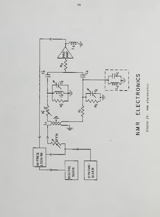
1 *
99
Co' (22 pF) to the low-noise preamplifier (Analog Modules LNVA-V) and
then detected. The resistance R., (120 fl) is necessary to kill parasitic
oscillations of the preamp and Lo ( 1 microhenry) blocks 60 Hz variations
of the preamp output. Tuning is accomplished by first setting C7 to
give the Larmour resonant frequency in the cryostat coil and then ad-
justing the "dummy circuit" component (primed) values to null the bridge
output. While extinction ratios as small as 10 were possible, tuning
stability typically limited this value to ~10~ 3,
Ideally, the noise level of a measurement involving a string
of amplifiers such as this should come entirely from the preamplifier.
However, without the above carrier cancellation scheme, the noise of the
high frequency lock-in detector is dominant. This is because the preamp
output must be attenuated to avoid saturating the lock-in. The signal
(and preamp noise) are thus reduced while the lock-in noise remains the
3same. Use of the bridge enhances the signal to noise ratio for He NKR
under typical conditions by a factor of six.
The high frequency lock-in mentioned above (Princeton Applied
Research 5202) represents the third modification to the Rollin scheme.
Although not quantitatively characterized here, the use of phase-
sensitive detection greatly enhances the sensitivity of the spectro-
meter. The vector sum of the in-phase and quadrature signals is the
final analog output of the spectrometer.
3.14 Ultrasound Electronics
The electronic system used for sound measurements is illu-
strated by Figure 30. It consists of means for sending a short sound
burst through the liquid helium and then detecting, amplifying, and
processing this burst to get either attenuation or phase velocity change
information about the medium of propagation.

100
COO
Oor
h-
oLU—ILU
3

101
A five megahertz synthesizer's output (Hewlett-Packard 3325A)
is gated and amplified by a Matec 310HP, which is triggered at 30 Hz
synchronously with the 125VAC line. The resulting output, 10 cycle
bursts of 5 MHz RF coherent with the pulse envelope, drives the trans-
mitting quartz crystal after attenuation to a peak-to-peak amplitude of
0.60 volt. The signal induced in the receiving transducer is amplified
first by a ham radio tuned preamplifier (Palomar P-308) and then by a
200 MHz wideband amplifier (Matec 625).
Different arrangements are then used to measure either atten-
uation or velocity. For measurements of attenuation, the amplified
received pulse is detected and filtered at 500 kHz. A boxcar integrator
(Princeton Applied Research CW-1) using a gate width of about 2 micro-
seconds and gate delay of 20 to 30 microseconds gives the average
voltage of the received waveform in the vicinity of the waveform maxi-
3mum. From this amplitude the attenuation of the He relative to that at
a reference temperature can be ascertained.
3Changes in the phase velocity of the He can be measured if
the phase of the received RF pulse is compared against a stable re-
ference (here, a PTS 200 synthesizer tied to the HP synthesizer).
Simply summing the reference and the received signal will give an output
which goes as the cosine of the angle between the two inputs. Unfortu-
nately, for changes in the input phase difference of more than a few
degrees, this cosine relation between output voltage and input phase is
a nonlinear one and even gives zero sensitivity at the and 180-degree
points. However, by using feedback, the phase of the transmitted signal
can be continuously adjusted to keep it near the most favorable point
(in terms of phase sensitivity) in relation to the reference phase.

102
Closing the two open switches in Figure 26 adds the reference signal to
the received pulse before detection and allows the boxcar output to
become the error signal for the phase controlling input of the synthe-
sizer.
The analysis of the resulting phase-locked loop is discussed
in Appendix A. From this analysis, one can see that the sensitivity of
the loop output to changes in the phase of the received signal is (from
(A10))
3V? 1
where a is the phase-programming co-efficient of the helium signal
synthesizer. For the Hewlett-Packard 3325A, a = 2.97 radians/volt.

SECTION 4
TECHNIQUE
4.1 Refrigeration
Demagnetization cooling is inherently a cyclic process unlike
dilution cooling. The period of this cycle for this experiment lasted
from several days to two weeks and consisted of the steps outlined
below. Magnetization of the 8T solenoid was typically done in about one
hour using a rate of increase of the central field of 2.7 mT/second.
The heat of magnetization of the copper nuclei typically resulted in
bundle temperatures of 60 to 80 mK. After about three days the dilution
refrigerator had reduced the bundle temperature to 28 to 30 mK resulting
in a heat capacity of 7 to 8 J/K. The heat switch between the mixing
chamber and the bundle was then opened and the bundle field was reduced
in three steps. First, the central field was reduced relatively rapidly
at 2.7 mT/sec from its initial value at 8.2 to 8.5 T down to 3.3 T.
This rapid decrease conserves liquid helium by reducing the integrated
heating in the upper portion of the magnet leads but does not appre-
ciably raise the bundle entropy as the resulting eddy current heating
occurs while the bundle is still relatively "warm" (>10 mK) . Second,
the field was further reduced from 3.3 T down to the neighbor-hood
associated with the 3He superfluid transition (.15 to .50 T) at the
slower rate of 0.27 mT/sec. Finally, the solenoid field was carefully
adjusted to place the He temperature just below T .
103

104
Over the week or two following the gross demagnetization,
minute step decreases in the solenoid field were made one to four times
per day to keep the nuclear stage in the vicinity of T . Although the
temperature remained within 3% of T during this entire time, the bundle
entropy was of course continuously increasing, with a resulting loss in
heat capacity. When the temperature drift rate had risen to an unac-
ceptably high level (or some other experimental contingency arose) the
bundle was remagnetized to begin another cycle.
4.2 Thermometry
Carbon resistance thermometers which had been previously
calibrated against a germanium resistance thermometer (in turn cali-
3 3brated against the He melting curve) were bolted to the He sample heat
exchanger body, the mixing chamber, and various other, higher tempera-
ture places in the cryostat. In addition, thermometers calibrated
against the exchanger body resistor were bolted to the bundle flange and
one of the heat exchanger struts. The two-lead resistances of these
thermometers were measured with a commerical AC-bridge (Linear Research)
and were used as general indicators for the timing of bundle magnetiza-
tions and demagnetizations and the general "health" of the dilution
refrigerator.
We determined He temperatures relative to T by two
3methods: NMR of platinum nuclei and NMR of the sample itself. He NMR
was used for all of the sound vs. temperature measurements while plati-
num NMR was used only for ancillary calibrations.
The susceptibility of platinum nuclei , which apparently fol-
lows the Curie law x a 1/T, (see Lounasmaa, 1974) can be measured by a
pulsed resonance method to yield a relative measure of temperature. If

105
the platinum metal is finely divided to give a large surface area to
3volume ratio the coupling of the nuclei to the surrounding medium ( He)
is fairly rapid owing to its relatively short nuclei-lattice relaxation
time T (t T = 0.03 sec«K). Our platinum thermometer is located close
to the region probed by the sound (see Figure 25) so that it can measure
the temperature of the central sample and also enjoy the magnetic field
homogeneity of that volume. The driving, amplifying, and detecting
electronics are contained in a commercial spectrometer (Instruments for
Technology) whose tuned circuits limit temperature measurement to fields
of 14, 28, and 56 mT. Typically, the spectrometer is configured to
drive the RF coil surrounding the platinum so as to give a "tipping"
pulse of < 10° from the direction (vertical) of the static field. This
tipping angle (actually a classical view of the particular distribution
of quantum mechanical spins with either "up" or "down" projections)
decays back to zero according to T . However, the current induced in
the RF coil after the tipping pulse is caused by the (classical) preces-
sion at the Larmour frequency of these tipped spins. The length of this
signal is governed by the effective nuclei-nuclei dephasing time x,
limited by our static field homogeneity to several hundred micro-
seconds. This signal, after amplification, detection, integration, and
subtraction of a small instrument-induced background, yields a number
whose magnitude is inversely proportional to the temperature of the
platinum nuclei.
2 3The perpendicular NMR shift v seen in He below the transi-
tion temperature T is very sensitive to temperature but apparently has
not been relied upon until now as a thermometer due in part to questions
of accuracy of the calibration information. Examination of the equa-

106
tions of Section 2.6 shows that, at any particular pressure, two cali-
brations are required: the products CA and CB. Here I will argue that
data already existing in the literature coupled with a few additional
measurements give a foundation for reasonably accurate thermometry in
the A and Al phases near Tc
for all pressures.
Leggett's (1974) prediction for the characteristic A-phase
shift frequency v is explicitly given by Equation (51) but this expres-
2sion includes the quantities e and <R >, which are not directly
measurable. If these two quantities are only weakly dependent on pres-
sure then, to an excellent approximation, the expression for the pres-
2sure dependence of the slope of v vs. temperature can be used with
o
e /k defined as 0.7 K and <R > equal to a constant fit to experimentalc
data. Figure 31 justifies this procedure by showing various groups 1
experimental determinations of f(P) (also listed in Table 2) as well as
points calculated from the theoretical relation (51) with e /k = 0.7 k
9 2and <R > = 0.70. This particular value of <R > was chosen in order to
cause the calculated values of f(P) to fall near most of the experi-
mental points. The data of Webb et al. (1975) may differ from the
others because of differences in temperature scales. As these problems
of temperature scaled have not been completely resolved (and may never
be as far as old data is concerned) the LaJolla data wre ignored for
2making the choice of <R >.

107
TABLE 2
2f(P) determinations, where v = f(P)(l-T/T )
Pressure (bar) f (P)( 10iJHz-) References
34.3 5.04 ± 0.02 Osheroff and Anderson (1974)+ Halperin et al. (1975)
21.5 3.8 Webb et al. (1975)
25.8 4.6
29.4 5.3
33 5.5
21.1 2.87 ± 0.20 Ahonen et al. (1976)
25.4 3.55 ± 0.1029.0 4.28 ± 0.2032 4.78 ± 0.20
23 3.17 ± 0.20 Giannetta (1980)
27 3.63 ± 0.20
2.05 0.57 ± 0.06 This work
Questions of temperature scale also enter into the calculation
of the theoretical f(P) from experimental data. Values of T
and (AC/C ) were interpolated from the data of Alvesalo et al. (1981)
and values of Npand F_ were taken from Appendix B of Wheatley (1975)
but scaled according to the more recent heat capacity measurements at
Bell Labs (Greywall, 1983). See Appendix B for details.
2Although the experimental determinations of the slope of v
3are sufficiently dense between 20 and 34 bar to calibrate the lie NMR
thermometry there, extrapolation to significantly lower pressures is
risky without at least one low pressure determination of the slope
2of v vs. temperature. Doing so at 2.05 bar in the 6 uk "window" of A-
phase created by a 28 raT field was accomplished by relying on the fact
that our residual heat leak is time-independent. In the refrigeration
3mode where small demagnetization steps are used to keep the He and

108
copper bundle temperature very near T and for solenoid fields B such
that the He heat capacity is negligible compared to that of the mag-
netized bundle, the temperature drift rate T is simply related to the
solenoid current I and its average rate of change I necessary to keep T
near T .
— = - = - (125)TBI K 0)
. 2Knowledge of I/I combined with a measurement of dv /dt then yields f(P).
2For NMR thermometry in or near the Al-phase using v one must
know the Ginzburg-Landau parameter 6 which measures the coupling of the
2up and down-spin gaps. The ratio of the temperature derivatives of v
in the A and Al phase is
(d VA/dT)
Al CA ( 1 - 6) flM .
2 =4CB
= 4 (126)
At the melting pressure, Osheroff and Anderson (1974) found
6 = 0.25 ± 5%. To my knowledge there has been no determination of <5 at
lower pressures although one would expect 6 to decrease at lower pres-
sures as it is a "strong coupling" parameter of sorts. Although I had
hoped to obtain low pressure measurements of 6, the narrow width of the
Al phase in our low fields allowed determinations of limited precision,
as the data of Figure 32 show. Nevertheless, this plot does strongly
suggest that < 6 < 0.25 is a good estimate at all He pressures. For
purposes of data reduction I chose 6 = 0.25 for all pressures. If 6
should indeed be as low as zero at the lower pressures, this would
result in the maximum possible Al phase temperature measurement error of
25%.
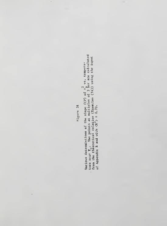

110
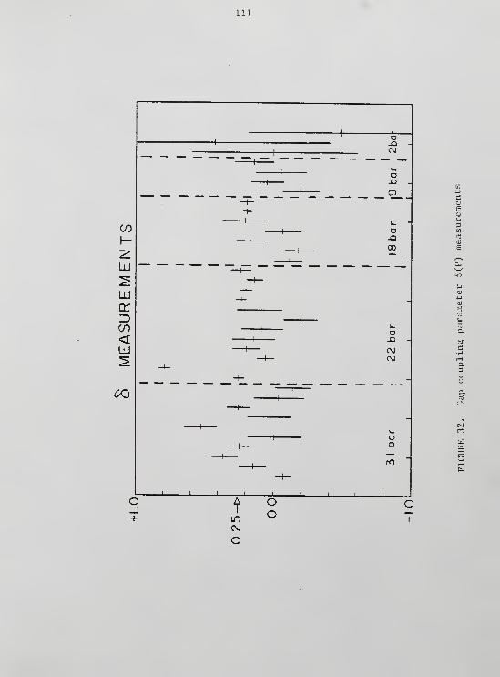
Ill
CO
LU
LU
q:
CO<LU
00
o
CM
o-Q
O
CO
O
ro
Q+ m
d
od

112
4.3 NMR in3He
3In typical operation the field B, produced by the He NMR coil
was ~3 x 10 tesla (~0.3 Gauss). Changing the static field and thus
the NMR frequency involved the following procedure (see Figure 29). The
persistence of the vertical field coil was broken and its current was
ramped toward the new field at ~2 x 10 tesla/sec. Meanwhile, the
frequency synthesizer, cryostat tank circuit, and "dummy" tank circuit
were tuned to the new frequency with the latter adjustment made last to
_3achieve an extinction ratio of < 10 . When the vertical field reached
the desired valve it was persisted. From then on, frequency and not
field adjustments were made to maintain the Larmour resonance condition
as the "background" field changed due to drift and effects of the bundle
solenoid fringing field.
Some fine tuning of the static field was done by applying a
weak horizontal field gradient. This did not significantly improve the
overall field homogeneity but did have a beneficial effect on the peak
structure. This structure, as seen in Figure 33, is caused by the
3homogeneity of the static field H(r) , weighted by the local He density
n(r) (which can be zero due to displacement of epoxy parts, etc.) and
H,(r), the field of the RF coil. The signal at a particular frequency u
is
S(u») - /d3r H (r)n(r)
TH(r) t2
1 + ( TH(r) - o))2T2
(127)
The horizontal gradient chosen was that which enhanced the "spike"
appearance of the central part of the lineshape , improving the precision
of the measured frequency shift, which was determined by fitting a

113
Oma -lOOma -200ma -250 ma
-300ma -300ma -400ma — 450ma
FIELD TUNING OF NMR PEAK
FIGURE 33. Field tuning of NMR peak

114
parabola to the tip of this spike. Figure 33 shows a series of line-
shapes obtained at different gradient currents. In this example -350 inA
gives the best shape for "tracking" purposes.
4.4 Ultrasound Signals
The excitation voltage amplitude (0.60 volt peak-to-peak) and
duty cycle (2.0 usee every 1/30 sec) were chosen as a compromise between
heating and available output signal. Pulsing the transmitting trans-
ducer at a 6 Hz rate but at 15.1 volts peak-to-peak caused some 30 to 60
nW heating at ~1.5 mK, 20.5 bar (normal liquid). Assuming that this
heating is proportional to the input electronic power, the local heat
leak due to the transducers during data collection was then some 0.2 to
0.5 nW. How much of this is directly due to the vlscocity of He is not
known though this should be calculable.
Figure 34 shows an example of an averaged detected pulse
illustrating the boxcar window position in time relative to the received
signal. The structure following the "zeroth" echo is not quantitatively
understood but is apparently due to the coherent summation of successive
echoes enabled by the ringing of the quartz transducers. The boxcar
window was always placed in the vicinity of the first maximum to avoid
effects due to following echoes and also to avoid the spurious feed-
through signal as much as possible. This feedthrough signal, visible as
the portion existing before the first helium signal at 28 microseconds,
is apparently a sum of excitations caused by ringing of the tuned preamp
and the receiving transducer caused by capacitive pickup of the elec-
tronic transmitter pulse. Its magnitude relative to the "real" helium
signal is large for this example (2.05 bar) as the normal liquid atten-
uation is largest for low pressures. The amplitude of the feedthrough

115
signal was always only a few percent of the helium signal except near
the superfluid attenuation maximum at 2.05 bar. The amplitude depen-
dence of the phase-locked loop for velocity measurement (see Appendix A)
then became an overwhelming effect and denied the possibility of per-
forming A-phase velocity measurements at that pressure.
The relative magnitude of the feedthrough-induced signal was
larger when the crystals were driven at their next odd harmonic, 15
MHz. Because of uncertainty in the resulting data corrections which
might be required, no 15 MHz data will be presented in this thesis.
To indicate the linearity of the entire receiving chain,
Figure 35 shows a plot of signal output vs. input relative to the ampli-
tude at just above T at 21.53 bar. Nonlinearity is much less than 10%
until below a relative amplitude of about 0.3, again affecting only the
2.05 bar runs.
A small, periodic modulation seen in some of the velocity data
was found to be related to the air temperature of the screen room, with
the periodicity caused by cycling of the supplemental air conditioner
directed into the screen room. This coupling of the velocity data to
room temperature apparently occurred in the phase shifting circuit of
the signal synthesizer (Hewlett-Packard 3325A), which has a rated error
of ±1° phase/ 1°C. The amplitude of these room temperature-induced
oscillations was damped by a factor of ~3 by a passive low-pass thermal
"filter" added to the air blower input of the synthesizer.
3As a final note, no effects (due to the nature of He or
otherwise) caused by coupling of the NMR and the sound were ever
noticed. Tewordt and Schopohl (1979) have studied this possibility
theoretically.
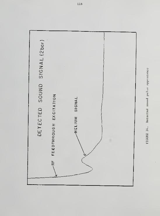
o
CM
116
CO
-)

117
3a.
li_

118
4.5 Data Acquisition
Recording the information contained in the He NMR and ultra-
sound signals included conversion of the analog signals to digital form
and some "real time" data reduction. The entire process followed a two
minute period timed by the digital ramp sweeping the static NMR field.
The various states of the system during this two minute period are
illustrated by Figure 36. The output of the digital ramp is shown at
the top of the figure. At the start of an up sweep, a trigger signal
sent by the ramp causes the 2-channel signal averager (Nicolet 1170,
actually only used for digital to analog conversion) to begin recording
the NMR and ultrasound signals (MEASURE mode). At the end of the 30-
second sweep, the Nicolet sends this information to the computer
(Hewlett-Packard 9845A) . This "READOUT" mode lasts 80 seconds due to
the slow speed of the BCD serial data transfer. After receiving the
data, the computer finds the highest NMR point and fits a parabola to
the neighboring points. The single number representing the fitted peak
location is recorded. The sound data, simultaneously accumulated during
the field sweep, are fit to linear function of time S(t). The value of
S(t) at the time represented by the NMR peak location is recorded. Data
files stored on magnetic cassette tapes thus consisted of up to 200 two-
component "points" at two minutes per point.
Data taking commenced after demagnetizating the bundle suffi-
ciently to cool the He to .99 Tc
. After an equilibration time of 30
3minutes , the He temperature drifted linearly up toward T over the next
several hours. Points were accumulated above T to establish datac
baselines before stopping data acquisition. Calibrations of the sound
signal were performed at least once at each pressure at just above T to
119
obtain data reduction parameters. Appendix C is the BASIC program
executed on the 9845A computer during data acquisition.

120
LU
<r3CO<UJ
J.
tzOk-oQUJ
cr
LU
Oc
3Oo<UJ
3Q.
U. CO

SECTION 5
DATA REDUCTION
5.1 Data Examination
A total of about 210 files of raw sound and NMR data were
stored on magnetic cassette tapes for these measurements, representing
approximately 3 weeks of actual data acquisition spread out over four
months. Of the 5 MHz runs (the large majority), about one third were
rejected upon examination of the data plots due to problems caused by a
high level of noise in the NMR data or an insufficient bundle demagneti-
zation. A smaller fraction of the remaining runs were rejected after
data reduction when it became evident that these runs had been done at
incorrect instrument settings.
For data reduction, each data file was examined and the point
nearest T , as identified by its signature in the sound or NMR data was
defined. This point plus a second, warmer point, typically defined an
hour later in the data, established a region of normal fluid data for
baseline purposes. Reduction of the NMR and sound data then proceeded
separately as described below and the sets of reduced data were after-
ward combined to give plots of sound dispersion vs. temperature. The
BASIC program used for data reduction is listed in Appendix D.
5.2 Temperature
3Before deconvoluting the temperature of the He sample from
the measured NMR shifts, some corrections for systematic errors had to
121

122
be made. The first correction dealt with the uniform change in time of
the NMR frequency caused by decay of one or both of the persisted sole-
noids in the cryostat. A baseline defined by a linear fit to the
defined normal region was subtracted from all of the NMR data. The
effects of a comparable relaxation change seen shortly after persisting
the bundle solenoid were avoided by ignoring any data taken in a period
of about an hour following the persistence of this solenoid.
The second correction dealt with discontinuities in the NMR
data apparently caused by changes in the positions of large iron objects
in the neighborhood of the cryostat. The data were corrected for these
"jumps" simply by requiring continuity at the dislocation and adding an
appropriate constant to all of the points to the right of the disloca-
tion. Such a "healing" process, required an average of about once every
10 hours of data, was usually extremely successful as judged by the
smooth appearance of the data afterwards.
After performing these systematic corrections, the magnitude
2of v, was calculated and from this the temperature was deduced. The
A2
relation between v and the actual data, namely signal averager ad-
dresses , can be derived for field sweeping as
VA
= 2vyH (n-nJ/N + [yH^n^ J/N]2
(128)
Here, the signal averager records the NMR amplitude as it steps through
N addresses. During this time the static field is modulated by the
total amount H . (n-n ) is the address difference of the shifted peakz o
from its location at T and v is the constant frequency of observa-
tion. For this experiment, the second term of Equation (128) was
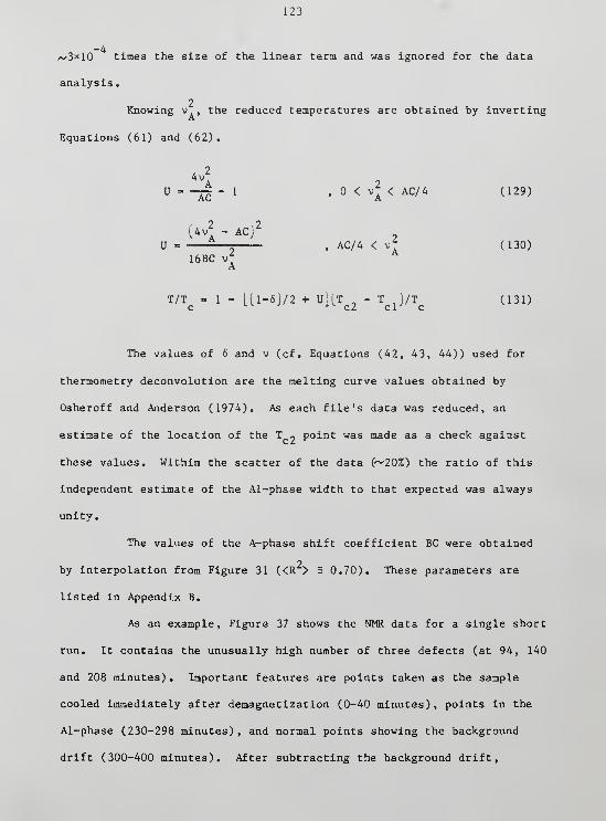
123
-4^3*10 times the size of the linear term and was ignored for the data
analysis
.
2Knowing v , the reduced temperatures are obtained by inverting
Equations (61) and (62).
24v
U=-^-l '0<v
l < AC/4 (129)
[^l ~ ACJ2
U = —, AC/4 < v; (130)
16BC vfA
T/Tc
= 1 - [(1-6J/2 + UJLTc2
- Tcl
J/Tc
(131)
The values of 6 and v (cf. Equations (42, 43, 44)) used for
thermometry deconvolution are the melting curve values obtained by
Osheroff and Anderson (1974). As each file's data was reduced, an
estimate of the location of the T ~ point was made as a check against
these values. Within the scatter of the data (~20%) the ratio of this
independent estimate of the Al-phase width to that expected was always
unity.
The values of the A-phase shift coefficient BC were obtained
2by interpolation from Figure 31 (<R > = 0.70). These parameters are
listed in Appendix B.
As an example, Figure 37 shows the NMR data for a single short
run. It contains the unusually high number of three defects (at 94, 140
and 208 minutes) . Important features are points taken as the sample
cooled immediately after demagnetization (0-40 minutes), points in the
Al-phase (230-298 minutes), and normal points showing the background
drift (300-400 minutes). After subtracting the background drift,

124
DHl 1 3 : T14 till?
1 3 T 3
125
healing the discontinuities, and dropping the first hour of data, the
reduced temperature vs. time is very nearly linear up to T . (U = -1)
where of course the thermometery no longer works. The greater scatter
of points in the Al phase (U = -1 to 0) is caused by the smaller slope
of the NMR shift there as shown by Figure 7.
Within the scatter of the data, on each run the temperature
drift T in the A and Al phases was always the same with no discontinu-
ity. This is at first surprising in light of the fact that the heat
capacity jump at T is split into approximately equal parts at T . and
T 2 by a magnetic field (Halperin et al., 1976). Apparently the heat
•3leak which caused T entered the nuclear stage via the He instead of
vice versa. This would be expected since t for the copper nuclei at
these temperatures is long enough to dominate the thermal relaxation of
the 3He.
5.3 Sound Amplitude and Velocity
Sound amplitude data were subtracted from a baseline defined
as the average of the raw data in the same normal region span used to
define the NMR baseline. Subsequent reduction of the data depended on
whether velocity or attenuation data was handled.
The calibrations of the voltages representing attenuation were
made by making two measurements at T > T that were 3dB apart and as-
suming linearity. The exception to this procedure was for the 2 bar
calibration, where the attenuation was high enough that the nonlinearity
of the measuring system became important. Here, the calibration was
defined as the difference between the normal operating value and that
obtained with no transducer excitation whatsoever. This definition
increased the accuracy of the high attenuation points at the expense of

126
the lower attenuation points. Since the absolute attenuation was not
measured, all measurements are referred to the attenuation at T .c
Calibrations of the sound velocity data were made in the limit
of small sound velocity changes Ac, where the relative sound velocity
change in a cell of length L is proportional to the shift in the re-
ceived phase of the sound after crossing the cell.
Ac —
c
The calibration between phase shifts and the output voltage of the
phase-locked loop was simply a matter of changing the signal synthesizer
phase by a known amount relative to the reference and recording the
change in the phase-locked loop voltage.
A third calibration defined the undesired effect of the signal
amplitude on the output of the phase measurement system (see Appendix
A). This effect was assumed to be linear in the amplitude of the
signal. The correction was a maximum of ~10% at the lowest pressure and
significantly less at higher pressures.
The deconvoluted data plots typically exhibit a knot of points
at T ,. This represents the normal liquid points which, due to the
absence of a real NMR shift above T , , were compressed into the region
near T ,
.

SECTION 6
RESULTS AND INTERPRETATIONS
6.1 Assumptions
Figures 38 through 49 display the coldest temperature run for
each of the different pressure and field combinations. For all of the
runs, the applied field H was parallel to the sound vector q. Ideally
this should limit the axis of the order parameter I to lie in the plane
perpendicular to H and q. Since the sound dispersion should depend only
on &*q, the theoretical results calculated for the perpendicular compon-
ents of the attenuation and velocity shift should apply.
To date, the only quantitatively successful attempt at fitting
experimental A-phase sound data is a series of rather involved numerical
calculations for 24, 26, and 33.5 bar (WSlfle and Koch, 1978). I cannot
say at this time if this scheme would fit our data. Certainly, it
cannot be directly applied to the Al phase as Wolfle and Koch assume
zero magnetic field. Instead, I will use the collisionless theory as a
guide for comparing the results between pressures. The Ginzburg-Landau
result for the magnitude of the energy gap will be assumed here
Cff-J2
'--T^ U-T/Tj (132)
c N
where it is hoped that all strong coupling effects are accounted for by
the experimentally measured heat capacity jump at T , (AC/C ).
127

128
£o\
o
Eo4-
©uc©
©
+*
6.02.05bar 143gauss
4.0-
2.0
0.0.992 994 996 998 1.000 1.002
FIGURE 38. Data plot: 2 bar, 14 mT
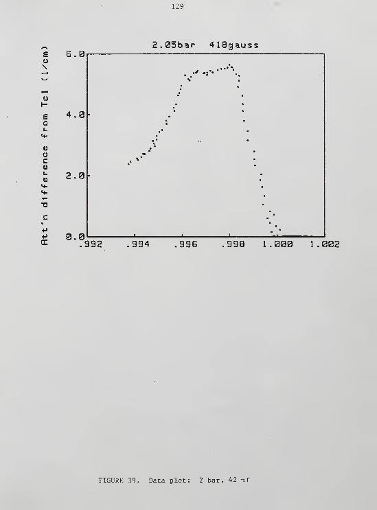
129
EO\
6.02.05bar 418gauss
* •:"*""*
*•.
u
£O
VacU(-
V<*-
4.0
2.0
+»
CE0.0
.992 994 .996 .998 1.000 1.002
FIGURE 39. Data plot: 2 bar, 42 mT

130
£O\
o
EO
«•
ouca
o«-
2.0
1.5 -
i.a-
9.15bar 143gauss
0.0
a -1000
SuN
QU
-2000
-3000
1 .002
.992 .994 .996 .998 1.000Reduced temperature (T/Tc)
FIGURE 40. Data plots: 9 bar, 14 mT
1 .002

131
£o\
o
£o
<*
Vuc•0
uo<*-
2.0
1.5
1.0-
9. 15bar 419gauss
0.0
a -1000
s(j\
eg
I -2000u
-3000.992 .994 .996 .998 1.000
Reduced temperature (T/Tc)
FIGURE 41. Data plots: 9 bar, 42 mT
1.002

132
18.19bar 143gauss
-3000
1 .002
992 .994 .998 .998 1.000Reduced temperature (T/Tc)
FIGURE 42. Data plots: 18 bar, 14 mT
1.002

133
o\
£os-
«*-
sucoi.
o«t-
1.0a-
.75
.50
.25
18. 19bar 286gauss
.00
a -1000
-3000
>*^'-
•••* **
fc
I ! ' Tgjfc" '
'992 .994 .996 .998 1.000 1.002
0, ji-*
.992 .994 .996 .998 1.000Reduced temperature (T/Tc)
FIGURE 43. Data plots: 18 bar, 29 mT
1.002
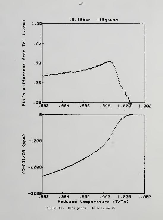
134
18. 18bar 419gauss
-3000
1.302
.992 .994 .996 .998 1.000Reduced temperature (T/Tc)
FIGURE 44. Data plots: 18 bar, 42 mT
1.002
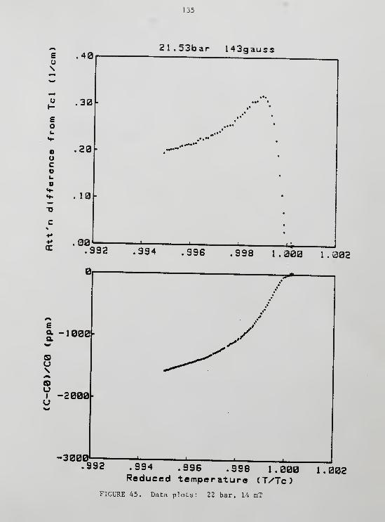
135
21.53bar 143gauss
-3000.992 .994 .996 .998 1.000
Reduced temperature (T/Tc)FIGURE 45. Data plots: 22 bar, 14 mT
1.002
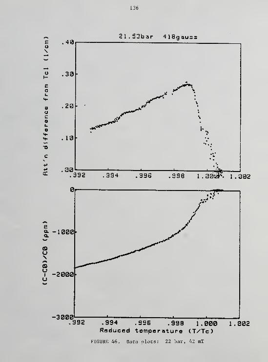
136
£o\
o
Eoi.
<•
oc9t.
o<*-
.4021.S3bar 418gauss
. 13-
.33.392 334 .396 .338 1 . aadF. 1 . 302
a -1000OnW

137
31.12bar 143gaus:
-3000.392
1 .302
.994 .99S .998 1.000Reduced temperature (T/Tc)
FIGURE 47. Data plots: 31 bar, 14 mT
1.002
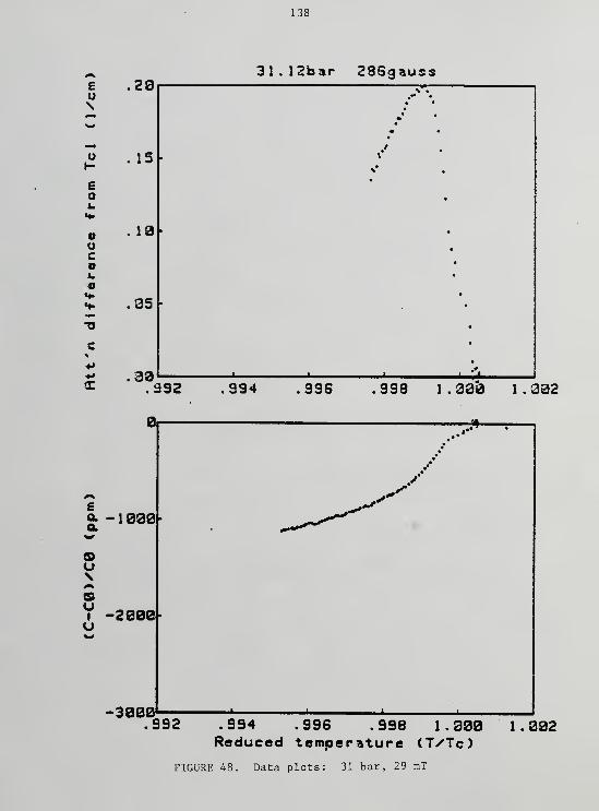
138
u\
oI-
£oi.
«f
ouc9
©
.28

139
u»-
EO
ucoft.
o«»
c
.23
. 15
. 13
.35
31
.
12bar 417gauss
.30.392
a
140
6.2 Attenuation
The simplest characterization of the A-phase attenuation data
is made by a list of the heights and temperatures of the maximum atten-
uation peaks. Since no significant systematic variation of those
quantities as a function of magnetic field strength was seen, average
values at each pressure can lump the 14, 29, and 42 mT data together.
The collisionless theory says that the sound attenuation
should be
a !*£J im(x) (133)
c FSkT
o o c
where k is a universal function of (A/lfioj) only. If one interprets the
maximum attenuation peak at each pressure as being caused by the same
value of x (e.g. x(l/l»23) for the clapping mode) then the heights of
these peaks should scale as the prefactor of x in Equation 133. Figure
50 shows a plot of the peak heights divided by the appropriate factor,
essentially a plot of the "experimental Ln(x)" vs. pressure. Consider-
ing that the peak height increases by a factor of 30 from the highest to
the lowest pressure, this scaling works remarkably well. The "experi-
mental Im(x)" values are significantly smaller than the collisionless
theory prediction. The clapping resonance of Figure 50 has its maximum
at Im(x) = 1.08 whereas the experimental data lie in the range of 0.17
to 0.33. This discrepancy could be explained qualitatively by invoking
the "smearing out" effect of quasiparticles with finite lifetimes.
Unfortunately, at the lowest pressure, one would expect only a fourth of
2this smearing effect as exists at the highest pressure because of the T
dependence of the quasiparticle lifetime. Much more cannot be said
without numerical calculations to include these dissipation effects.

141
If the attenuation peak maximum is indeed due to the clapping
resonance then T/T for this peak should result from inserting
#u) = 1.23A into Equation (132). Figure 51 is a plot of this theoretical
value and the experimental results vs. pressure. The agreement is good
only at low pressures. From the numerical plots in Wolfle and Koch
(1978), the location of the a peak is apparently little affected by the
inclusion of dissipation. For this reason, quasiparticle lifetime
effects may not explain the peak location discrepancy. Problems with
input data for the thermometry calibration could be suspect but it
should be noted that corrections to (AC/C ) or kT shift both the exper-
imental and theoretical points in the same direction. Another possibi-
lity is that specular reflection in the sound cell significantly mixes
in the attenuation components important for i«q * 0. For example, the
peak in a occurs at a temperature 2.4 times colder than the a peak due
to clapping, about the ratio of the discrepancy for the high pressure
data of Figure 51. The data of Paulson et al. (1977) also show 5 MHz
attenuation peaks which are "too cold" but the discrepancy is less , only
about a factor of 1.7.
The attenuation peak at 2.05 bar shows a distinct twofold
structure near the maximum attenuation. This feature was also seen in
horizontal fields, for q*H = 0. It may represent structure masked at
higher pressures due to quasiparticle collisions such as a contribution
by a . Another possibility is that the extra peak is an artifact caused
by a combination of RF feedthrough and the rapidly changing velocity of
sound in this region. Such a "beating" effect is quite possibly the
origin of the attenuation satellites seen in the B-phase at low pres-
sures (Paulson and Wheatley, 1978).

142
Oro
O
OJ3
- O
„(XD%X) w| 1VlN3WI«3dX3„
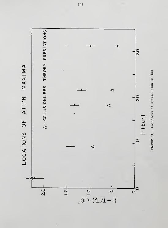
143
CO
O<oo
co

144
The effects of the Al phase on the sound attenuation can be
easily seen in most of the data at 42 mT. The rounded shoulder appear-
ance is apparently a separate attenuation peak, starting to separate from
the main peak as suggested by the higher field data of Lawson et al.
(1974).
6.3 Phase Velocity Changes
The rate at which the sound velocity drops below T from its
normal liquid value increases by roughly a factor of two on going from
the highest pressure (31 bar) to the lowest pressure at which a velocity
measurement was made (9 bar). The low temperature limit of this veloc-
ity drop is expected on theoretical grounds to be the first sound veloc-
ity C,. However, an attempt to scale the velocity runs by
(C - C,)/C did not work very well. Turning again to the collisionless
theory for superfluid sound dispersion, the velocity change near Tc
is
seen to be proportional to the gap for T near Tc
(cf. Equation (110)).
C " °0 _ A(T)
°0 F® kTc
This suggests a scaling by the factor
1/2
A(AC/C
N)
1/2
(134)
F* kT (1 - T/T )
1/2F*
c c U
(135)
Figure 52 shows that such a scaling is approximately valid.
The shape of the velocity vs. temperature curves is qualita-
tively different from the zero sound picture, which predicts exactly
zero shift in the velocity for temperatures above the pair breaking
limit tfw = 2A(T). Although the shape of the velocity curves initially
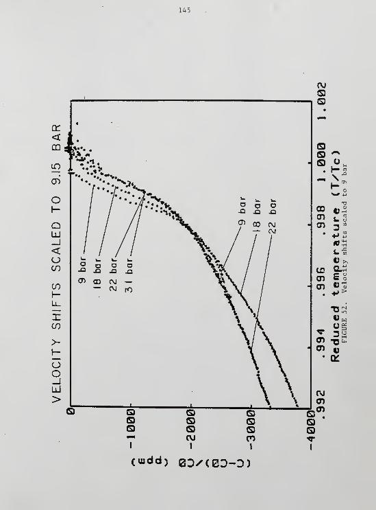
145
CD Q

1/2suggests it, fitting the curves to a constant times (1 - T/T ) ' was
not successful. For lower temperature data ]Aw«A, where the velocity is
expected to go as the viscosity, such fits might be possible.
There may be a connection to viscosity in the Al phase veloc-
ity data. The shapes of the reduced viscocity plots in finite fields
(Alvesalo et al., 1975) are suggestive.
The lowest pressure data at 9 bar seems to suggest little or
no drop in the velocity above To.
6.4 Metastability at the AB Transition
At the lower pressures of 2 and 9 bar, the first-order char-
acter of the transition between the A and B phases of superfluid caused
hysteresis in the location of the transition temperature T^. Figure 53
shows a particularly clear example of supercooling and superheating at
9.15 bar in a 14.3 mT field. The upper and lower plots are raw data vs.
time for the NMR and ultrasound signals respectively. The temperature
as a function of the time first drops after the initial bundle demag-
netization, "turns around" at 30 minutes, and then warms at 40 nano-
kelvin/minute, passing through T , at 212 minutes.
As the sample warms, the B-phase exists between 62 and 154
minutes. This is marked by both the NMR and sound data - the later
transition occurs very near the sound attenuation maximum and the re-
sulting amplitude jump in the data is small. These sound signatures,
plus the different slope of the B-phase NMR, eliminate the possibility
that the NMR jumps were caused by a pertrubed static field as was the
case for Figure 37.
The temperature for the B to A transition occurs in this run
at about the same place for runs without A-supercooling so it is not

147

148
clear that the B-phase is superheated here. The degree of supercooling
of the A-phase is comparable to other measurements (e.g. see Wheatley,
1975) but the apparently unprovoked A to B transition is an unusual
feature. It may be significant to note that no highly magnetic solid
3such as He or CMN refrigerant was in direct contact with the sample.
Also, the immediately previous history of the sample before this run
started included about 80 minutes at ~-1.001 T ,
.
cl
6.5 Summary and Future Work
The two chief results of these experiments are a practical
3demonstration of He NMR as a superfluid thermometer and a systematic
3comparison of low-frequency zero sound behavior in superfluid He-A with
the collisionless theory over a pressure range of 29 bar. In parti-
cular, the pressure scaling of the sound attenuation and velocity is in
fair agreement with the collisionless predictions. The temperatures of
the attenuation peaks show a major discrepancy, especially at high
pressures. This discrepancy, about a factor of 2.4, is the same as that
observed by Paulson et al. (1977) if their temperature scale is the one
which produced their NMR shift data on Figure 31.
Other features observed in the data include a double atten-
uation peak at 2 bar and strong supercooling of the A-phase at low
pressures. The data for the Al phase awaits theoretical explanation.
Extensions of these measurements in the future should gather
data at new pressures, magnetic fields, and sound frequencies. The
pressures between 2 and 9 bar and in the vicinity of the zero-field
polycritical point would be interesting; the former because of the
apparently qualitative changes in the sound attenuation which take place
there and the latter because of the possible "step" structure in the
149
data of Figure 50. Different field orientations could be used to deter-
mine the importance of the contributions of x. and X (see Wheatley,II c
1973). Finally, attenuation measurements at the next transducer har-
monic, 15 MHz, would allow comparisons with the experimental work of
other groups, in addition to those made here at 5 MHz.

APPENDIX A
PHASE LOCKED LOOP ANALYSIS
Figure 54 shows the various phase shifts in the loop involving
3the two synthesizers, the He sample and the amplifying, summing, and
detecting electronics.
The various phases are
9 = reference synthesizer phase
9 = signal synthesizer phase
9_ = phase of signal after passing through cables, amplifiers,
transducers, and sample cell
The various voltages are
Asin(ut+9 +9 ) = signal input to adder
Bsin(o)t+9 ) = reference signal input to adder
V, = AC-coupled output of detected signal to boxcar
V = boxcar output which controls signal synthesizer phase
Since the duty cycle of the pulsed signal is extremely low, the AC-
coupled output from the detector to the boxcar is just
V1
= [A2+B2+2ABcos(9
1-$ +9
3)]
1/2-B (Al)
The output of the boxcar is
150

151
V2
= CV, , C=constant (A2)
which controls the phase of the helium signal synthesizer via the rela-
tion
9j =<t»Q +aV
2,
$' = constant (A3)
Using (A2) and (A3) in (Al) gives
V2
= C [A2+B2+2A3cos(<))
(
!
)
-(t) +aV2)]
1/2- B} (A4)
In the ideal limit that B>>A, (A4) reduces to
V2
= (CA/B)[A/2+3cos(4>J -9 +<J>3+aV
2) ] (A5)
With the loop locked, the quantity in brackets can be set near zero
volts. This, plus the requirement that B>>A, allows me to set
cos(^ -<t> +4>3+aV
2) ir/2 - (^ -9 +<l>
3+aV
2) (A6)
Inserting (A6) into (A5), the output of the loop is seen to be
V2 " TTTlk) LA/2-B(^-Vh- */2)] (A7)
The dependence of V2
on changes in 9_ (and therefore on changes in the
helium phase velocity) is simply
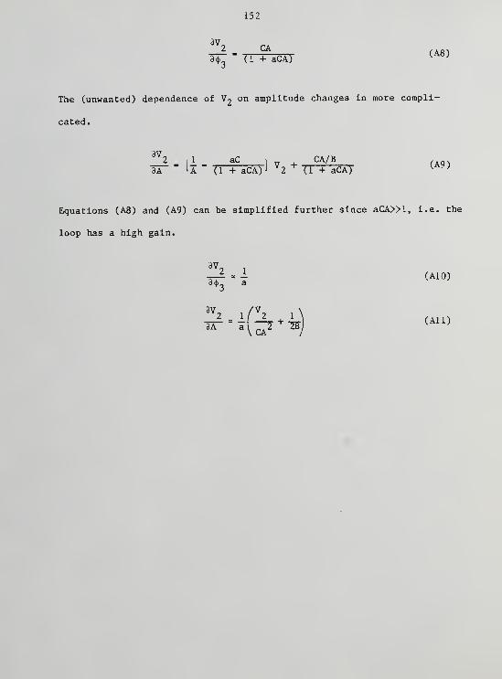
152
3V
"3^"=
(1 + aCA)(A8)
The (unwanted) dependence of V2on amplitude changes in more compli-
cated.
3V_A = li ,
aCi
CA/B3A U (1 + aCA) j
V2r
(1 + aCA)^' J
Equations (A8) and (A9) can be simplified further since aCA»l, i.e. the
loop has a high gain.
9V2 1
TT- ~~ 7 (A10)8*3
a
3
^-ii +^

153
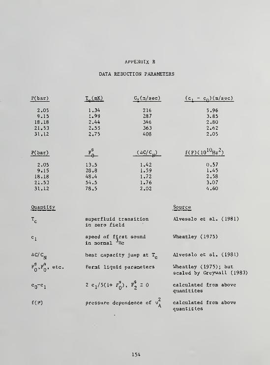
2,

APPENDIX C
DATA ACQUISITION PROGRAM
1101:0130140150166170180190206210220
300310320
L»=i nodi fickt ton on 30 jPEftl 4 t s fortliti .Jig
k-*x- posn ion of high* si (imp ,-.,-.,,
Y«*x«.,*lu« ot highest nmr point
v'"-;, 1l%rf,n4 '3 i6— ^0-Mo„n, ,n SHORT ,.:.r,,
OPTION £:*?.£
PIM Co«ff<4),Xi 200>.V<200)
COM INTEGER lh.:.,s„K4097;i>* »i pia 1 1. i on . s ound uo I • »o*" stor mg >licol«< l l 70 r ».".
<
INPUT -Ciw, th. f,rst I.hTh fit* ,-,„,- - --
INPUT "Ci W« nu.ber of ftl*. rMu,„H ,
! C2«,n,po,nt>-.200po,n, , %, *'* ™n«.Hn
L INPUT -C*« tod*. , (»„.,,„,-"•'" '"-
4004 10420
4 704664 90500510520530540550
:T14'
' Th,i sect, ion = *.; ..,„ PiEXIT GRAPHICSIF n =oc».|,- , i.: them STOPFi l*«»"M a &VRLs<=0*1
IF = 00*1 THEN Zii)WRITE 10 11.-; I
WRITE 10 11, Si 3CREATE Fi UJ.200.20ASSIGN »1 TO Fi U*PRINT »l:I'uf,H»vREAD »1 ,
1
WRITE 10 U.6; 10PRINT -Start JO second WAIT'
FOR 1=1 TO SWAIT 10000-NEXT I
PRINT "End SO second WAIT"GOTO 640
'T«ll Mice'2-STOP i=
'200 point
o STOP
SHORT r,ui,,bir
ui nd to begii
IEASUP E uod€
' Repos i ' i on poi m,-rIM-iks Htcolet READOUTIHatt >ihi le Nico 1 do-
155

156
570 !
580 CREATE Fi let, 200,20590 RSSICH »! TO File*600 PRINT »l; Dummy610 READ m, i
S2fl !
630 i
640 PP INTER IS650 PRINT • "
660 PRINT File*,"RFB-S",Date*670 PRINT '• ••
630 PRINTER IS 1£690 i
700 i
710 P»l720 Input: ..-ALL Dunp730 Vi»in = -'00
740 Ymax=-i>7i£:3750 ::«i,so760 Moi..*r.t*0
770 !
100 points, 5 SHORT nunt
'- iuie t ape t
.
: , ,.,, n<IPepos i t ion point*,
'Lite l hard
beginning of fi•"' U beginning
.,c 'iun '--' 'he point nunber
!»unp READ; the Hicoln outputs "bii«Iin«" for Moment
teetion finds rh« nhp peat Ohigheais' HOfasnt of sorts.FOR 1=2 TO 2039 ,..
I'.'.' data transmissionIF Hi.:«,«r,,W;,,i,,i- THEN GOTO S50:'.n*x«I
Ynax*Nici.en«, I
IF Nienenvix Vnin THEN C0T0 870Flon«nt"Mon*nt*- Niencn., I -Y,„in •-!NEXT I
on c a 1 •: u I at. ,- 1 t n€ MH p pe 4"* peak •» ip".1
I par i: tn« nu1 Appro;: l matelv
a-:=Iparl !ftuoid problems
??e i
300 ! ;
310due t<
320330340350360370880 ! ;
890 '
900 i
910 !
920 !
930 ' The fol lowing = * : r ,
940. i a parabola thro. ion950 Ipar=50960 I par 1=INT' ( Ipar-1 '.:•"
970 IF Xi,.ax<Iparl THEN ~.„
930 FOR 1 = 1 TO I par990 X<I>-I-Ip*rl1000 mj-NicnenOInax-I-Iparl101 o ne::t i
1020 N= I par1030 Deor.€e = 21040 CALL Pol -non i a I > r;- » >
.
.F, Dfreg. Dfre« . lift ot . Abort1050 :;r„au=-i;oef f ( i > t2*Co«1060 CPtLL Pplot.' Ipar. Ipar '
1070 '
10S0 '
1890 !
1100 !
1110! This i*c
1120 1=11130 FOR J=2049 TO 4083 STEP 11Avoid the end point1140 ::••
i . = j
1150 vi;=ii, CM ,n:, i ...
1160 1=1-11170 ti*i
U30 ne::t jU90 Degree»l1200 CALL Pol '/nor,, i al • ::.
F, Dfr*g, Dfres. Dftot . lib
1210 Ye«Coeff<0>*Co«f f<l)*<x»ax*2048>1220 !
1230 !
1240 !
1250 !
1260 ! FOR 1=1 TO H
1270 ! PRINT "POINT »*, I , X< I) , Y< I>1230 ! NEXT I
1290 !
:ul at es
jo i d i n i
:*' Iparsed f nmp
, N. Degree, '*> .Regss, Resss, Total = = . Regns . Resns
LD i sp 1 a*
p ar abo 1 a pe ak
P i : i s
f<*>,N,Begr
.'Use "11" to
•aioht 1 m« f i t
,P-egss. Resss .Total ss,P*<
aoe sound phase shi
, Pes in:
peak

157
1JUU
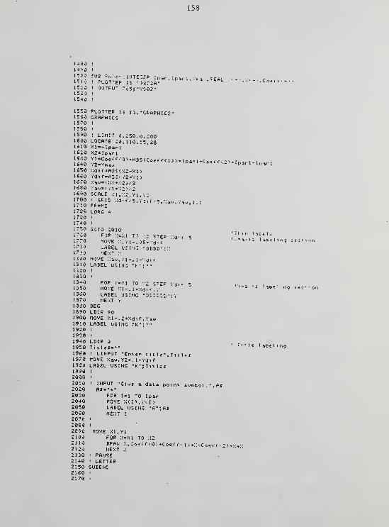
158
152315301540
SUB Fpl.;.' • INTEGER Ip1 PLOTTER [3 »?S?2A"1 OUTPUT 705; "VS02"
PLOTTER- IS 13. "GRAPHICS'GRAPHICS
1570133015961600Id 10
16201630164016501660167016301690170017101720173017401750i7-:o
177017301790130013101320133013401350I860137013301390190019101920193019401950I9601970193019?0200020102020203020402050206020702080209021002110212021 iO2140215021602170
' LIMIT 0.250.0.200LOCATE 20, 110. 15,35XI— I pariX2 = Iparl
•n"C©«ff<0>-ABSCCo«ffu>>*i parl <
Y2=Ym»xxai i'»aeis<x2-xi >
Ydif"ABS(Y2-Yl
>
Xau-0!lfX2>^2Yiv»c YlfY2>.-23CALE X1,::2,Y1.Y21 GRID :5dif/-5,v.jiv.-5. ::»... ,».• 1
i
FRAME "
'
LuRC 4
GOTO 2010POP x = ,;i to ::2 STEPmove ::.vi-.05-v.3 , (
'
LABEL USING "DDBD" :
'
NEXT Amove :: a.,,vi-. i-v.3,fLABEL UilllG "t •; ••••
FOP y»Yl TO V2 ;.TEPmove :;i-. i-::,3 ,t ,-,
LABEL USING "DBfiCDD 1
NEXT VDECLDIR 90MOVE Xl-.2*Xdif , YiwLAEEL USING 1'K";""
LDIPTitle*-""! LINPUT "Enter title",MOVE Xav, Y2*. l*YdifLABEL USING "K";Title*
INPUT "Give a dili point iyoto 1
.
"
.
hiA*»"*"
FOP 1 = 1 TO Ipir-MOVE XCI>,Y<I)LABEL USING "A"; A*NEXT I
MOVE X1.Y1FOR X=X1 TO X2DPAU X.Coeff <.0>+Coe» " i l)»X*CQeff < 2>*X*Xnext :;
~ '
1 PAUSE1 LETTERiUBENB
1 - I p ir 1 - 1 p ir 1
Ti'U libel

159
2130 '
2190 !
2200 SUE Polvno«i4l<X4*),Y<*) N D--,r-- r|F,I>0»g,Dfr* s .l>ftoi. Abort)
'"' B<9ree,Coeffs<*>,R«g;35. fu iss, Toi »Us.R*g*4 ,R*si»i2210 ON ERROR GOTO Eorub2220 Abort »62230 OPTION EhSE22-40 DIM Mitr i :;( D*ar" ninr».i t_ r.
2250 RESIH Co.ffstS^r..!*P€ *'- In "'
I)«9-«.»«9r««^E.D. 9 r, € .
2260 IF tl*ar»e >N-2 THEN -MPF'-TT i,- . ^
2270 Bfr*g=r,egPeeSUBEaIT Check for higher decree th*n possible
2230 Df res=N-l-Degre*2290 Dftot»Dfreg*Dfres2300 FOP K«0 T0"D»gr*» , .-
2310 FOP J«K TO I«9rtiUP -"" ^,9," c'» tqu**io»w
2320 H»trix<K. J;=02330 FOR I»l TO H
till Mtx;~" t *<«.«-"»r 1 x<IC.J>^NS<K>^IIC<J)
2350 n«rix<J,K>-H*tris«<K.J)2370 NEXT J
2386 B<K >»92390 FOP 1=1 TO N2400 BCK>-B<K>*Y<I>*FMC<IC)24 10 NEXT I
2420 NEXT K
2430 MAT [nu-IHV(N*tri*)i -,,
2440 MAT Coeffs»Inv»B syste« of equations2450 FOR I«| TO H2460 :<l=.:i»::. | )
2470 ;!2-X2*X<I>»xci,2480 Y1«Y1*Y' |
,
2490 Y2-Y2+V li-VM,2500 2>3>X(I)*Y(I)2510 NEXT I
2520 Y1*Y1'N2530 X1=X1N2540 Total SS»Y2-N»Y1*Y12550 Q03UE Regs*2560 Resss*To> alss-Regss2570 Pegrui = R#gsi--Dfr*o2530 ResBS'Resss/'Dfres2590 OFF ERROR2600 DEFPULT ON2610 F'Rtgu/RtMl2620 DEFAULT OFF2630 SUEEXIT2640 Pegsi: Regsi»02650 FOR I«l TO N2660 J=02670 FOR L»0 TO Degree26S0 J=J+X(I>-L*Coeffs<L)2690 NEXT L27O0 Regss-Regss+tJ-Yl)-?2710 NEXT I
2720 RETURN2730 SUBEXIT2740 DEF FHG(M>=X.'n-M2750 Botub: fibort=i2760 SUEEND2770 i
2730 i
T.:

160
279828002S102S2023302340235028682370288823902900291029202930294029502960297029302990300030103020303030403050306030703030309031003110312031303140315031603170313031903200321032203230324032503268
SUE Dump1 Dump is i Modification of Dor, Bakalyar's program for reading! Nicolet data. Instead of expl tcitelv telling the Nicole* to1 READOUT, the 9345 "listens" and the Nicolet "talks" as soon' it has done one su«en (Nicolet SUT0CYCLE mode/. dec as i on all •
1 the Nicolet fails to "talk": it's then "kicked" Cexpl i c i t«1»>. told to READOUT -
'.
COM INTEGER Ni c memv 405
;;x»i
ON ERROR GOTO 3120
1 URITE 10 ll,6;3CONTROL MASK 11: 1
CARD ENABLE 11OUTPUT 11 USING "*,E": 52CONVERT 11: "I", - '• TO ". "
PEM This conversion is neceiPEN made 'he minus = i .jn ins'PEM as the del imi t*r.CONTROL MASK 11:0 '
CARD ENABLE 111 WRITE 10 1 1,6: 10GOTO 3230
!Kick counter'Looking for ERROR 20 in ENTER Nicmen
!T«11 Nicolet to STOP,i Ne <t i.,ord from 9345 i
Changes space to comma indat a from Nicolet.
•••. If conversion is not1 of the spac* is recognized
• s USAPT for receiving da- a.
!T*H Nicolet to READOUT.
! This section "kicks" 'he Nicole', it" it fails to READOUT! and dives ERROR 20.PPINTEK IS 3
PRINT "ERROR in Dump subprogram"PRINTER IS 16URITE 10 11.6:3 !T*11 Nicolet to STOPURITE 10 11,6:10 !Tell Nicolet to READOUT (again!Xx*Xx+lIF :;x>10 THEN 2928 'Allow only ten "kicks"
ENTER ll;Niem«m'.0
URITE 10 11,6;15SUEEND
! D at a transfer from Nicolet to! using f reef
i
eld format.IFrees Nicolet

APPENDIX D
DATA REDUCTION PROGRAM
10203040506670809010©1 10120130140150160170ISO190200210220230240250260276230296300310320330346350360378380396400410420430440450460470480490500510520530540550560570580590
Last modification on 11 October 1983.TC6 reduces data taken using PEAKX <X> l> . A-phase NMR shifts are convertedto reduced temperatures. Sound velocity phase shifts are changedto normalised sound velocity shifts and amplitude data areconverted to normalized attenuation values.
SUE Linear: first-order fit to data.SUB Average: zero-order fit to data.SUE Dp lot: sets up graphics for plotting data.SUE: Points: displays point values near indicated point.Hertz used instead of radi ans'second.
Ref.l*J.C. Wheat u v . Rev. Mod. Phys. 47, 413 •1975'..Ref.2«fl.I. Ahonen et al., Journ.Low Te»p. Phys. 25, 421 <1*76'F:ef .3=D. H. Osheroff andP.U. Anderson. Phy*. Rev. Lett .33,686 C1974)p€t.4=W.F. Brinkman, J.W. Serene. P.W. Anderson. Phy s. Rev. Al 0. 2336 <1974>Ref.5=T.A. Alvesalo et al . , Journ.Lon Temp. Phys . 45, 373 '.19*1'
OPTION BASE!Miscellaneous string variables: File*, A*
1 Ne-;t line holds experimental data variable3H0PT P<200:. ,Xmax<200>,Ymax,Xmay<200 ', Ye^Oe1 Next four lines hold input parameters forSH0PT Fsound,L, Gamma. A 1 pha, Del t
a
INTEGER Day, MonthCOM Attn*SH0PT Hsweep.HnmrSHORT Pbar, Tc , C6, Nua2, 22, 23,24' Ne-:t line holds parameters derived from inSHORT 21, Al, Be, He! Next three lines hold plotting variablesCOM SHORT XK5>,X2<5>,Y1<5>,Y2<5)INTEGER 0, 15, 16, 17. ISDIM >;iab*C50J, Ylab*C50],Tit 1 etc 50]1 Ne--t four lines hold variables for NMR anaSHORT X»«y0,Ftc2,X«>ax!,Fshift<2ee>,U<20e>INTEGER Imin. I max, II, Itc2, Itcl. In, I gapINTEGER I guess, 1211,1212, I200, 1221 , 1222. I200REAL C1.C2,D1,D2. Anmr.Bnmr
1 Ne'-t line holds extra variables for soundSH0P T Asound, 25', 100/! Output numbers are the following:SHORT T<20e>,Cshift C206), Al rat i o, Udi
f
25*. Cold*
parameters
Fsound=5. 800E6L=6.25E-3Gamma=3. 2433E3Al pha=6. 4E-9
Sound frequency in hertzLength of (cold' sound pathg-factor in hertz per gau= =
Al width coefficient in lei.See Ref.3
NMR slope ratio parameter: ; Refs. 1,:
161
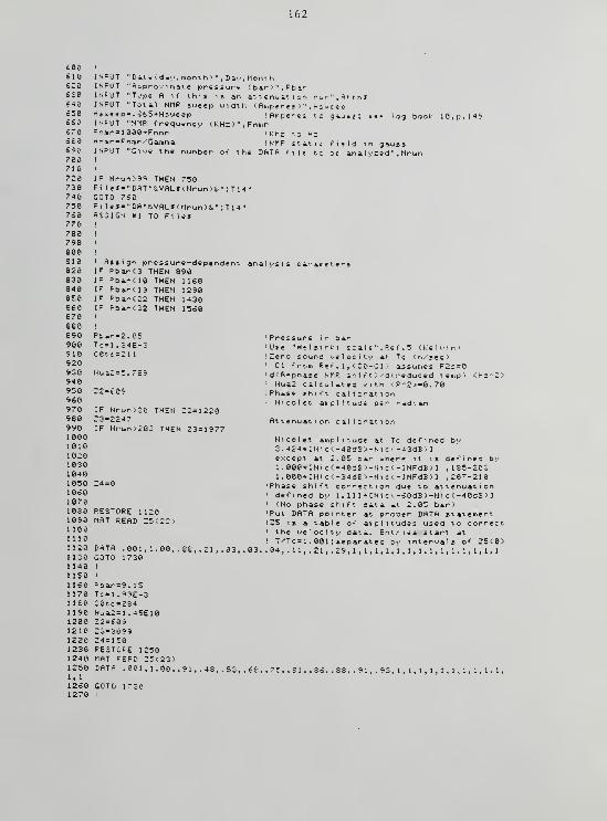
162
60Q610620630640650660670680690700710720730740750760770780790800810820830840850860870880890900910920930940950960970980990100010101020103O104O1050106O10701080109011001110112011301140115011601170USO1190120012101220123012412501.112*01270
I NPUT "Dat e C day . month >", Day, Mont h
INPUT "Approximate pressure <bar •
" . PbarINPUT "Type A if this is an attenuation run ".Attn*INPUT "Total NI1P sweep width < Amperes >", HsueepHsweep=. 865+Hsueep
! Amperes to aauss; see 1 oa book 10, p. 141INPUT "NMR frequency (KHz)",Fnr,,rFnmr=100O*Fnmr
! Khz to HzHnmr=Fnmr Gamma
! NMR static field in gaussINPUT "Give the number of the DATA file to be anal yzed" , Nrun
IF Nrun>99 THEN 750Fi ) e** " DAT "iVHLS < Nrun >&" : T14'GOTO 760F l 1
e*= " DA " 8.VAL* '' Nrun >t • : T14"ASSIGN #1 TO File*
1 Assign pressure-dependent analysisIF Pbar<3 THEN 890IF Pbar<10 THEN 1160IF Pbar<19 THEN 1290IF Pbar<22 THEN 1430IF Pbar<32 THEN 1560
parameters
Pbar=2. 05Tc=1.34E-:C0tc=21
1
Nua2=5.7E1
22=609
IF Nrun>323=2247IF Nrun>2
THEN Z
3 THEN
RESTORE 1
HAT READ120
DATA .001GOTO 1730
Pbar =
Tc-1.C0tc =
Nua2 =
Z2=6tZ3=3£Z4=i:PESTCMAT f
DATA
, 1.00, .38, .21, .03, .03,
IE 1250£AD 25<23),001. 1.00. .91, . 4S
Pressure in barUse "Helsinki seal e " . Fe f . 5 (
Zero sound velocity at Tc '. m
CI from Ref . 1 , CCB'-Cl ',• as sumdC A-phase NMR shi f t >-'d<reducNua2 calculated with <R~2>=
Phase shift calibrationNicolet amplitude per radia
Ke 1 v i r
sec )
At lenui i brat l or
Nicolet amplitude at Tc def3. 424* CNi c k-40dE )-Nic • -43dEexcept at 2. OS bar where it
1 . O00*CNicf-40dE;'-Nic C-INFd1 . O0O*CNi c C-34dB>-Ni c (.-INFd
Phase shift correction due t
defined by 1 . 1 1 1* CNi c i -60dE(No phase shift data at 2.0
Put DATA pointer at proper D
25 is a table of amplitudesthe velocity data. EntriesT'Tc=l . 001 ; separated by int
04, . 11 , .21, .29, 1, 1, 1, 1. 1, 1, 1
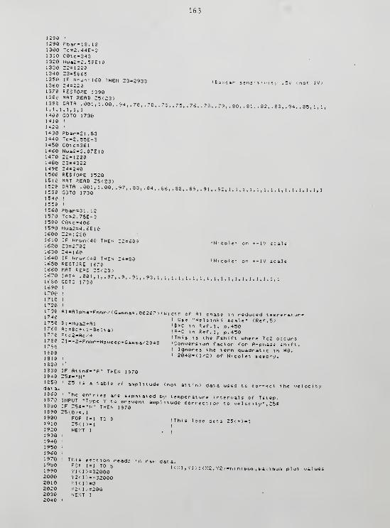
163
'Boxcar sens i t i v i t
'
1286 '
1290 Pbar=18. IS1306 Tc=2.44E-31316 C8tc=343132e Nua2=2.58E101330 22=12201340 23*58651356 IF Nrun<160 THEN 23=29331366 Z4«2201376 RESTORE 13961386 MAT READ 25(23)1396 DATA -001, 1.06. .94, .76, .70, .73. .75, .76. .78 79 80 SI 8^ 83 S41,1,1.1,1,1
'""'"1460 GOTO 17361410 i
1426 !
1430 Pbar=21.531440 Tc=2.55E-31450 C6tc=3611466 Nua2=3.67E161470 22=12201486 23=43221490 24=2461566 RESTORE 15281510 MAT READ 25(23)
1530 GOTO ;^' 1 -M" 97" 83 »- e*.-«,.88,. 89 1 .91,.«, l ,,, liltl|1 ,..»...,
1546 !
1556 !
1560 Pbar=31 . 121576 Tc=2.75E-31580 C0tc»4061590 Nua2=4.6E161600 22=12201610 IF Nrun<40 THEN 22=609162© 23=27021630 24=1601640 IF Nrun',40 THEN 24 =861650 RESTORE 16761660 MAT READ 25(23)
\tlt"""
; 111•
' • •97
> • 9 > • «• • w - 1 .
i.
i • i.
i , i,
i , i . i , i . i , i , i . i . i . i , i , i1 680 GOTO 1 7381690 !
1706 i
1710 i
1726 i
5V '.not IV)
.85,1, 1,
1,1,1,1
i~r
' N I C O 1 € 1 •IV scale
1736 Rl-Al pha'Fnmr " Si17461756 Bc=Nua2*Al1766 Ac=Bc*(l-Del ta;1776 Ftc2=Ac-41780 2 1 =-2*Fnr„r*Hs weep * Gamma/- 264 S1790180O1316 !
1826 !"
1336 IF Attn*="A" THEN 19701846 25*= "N"1850 ' 25 is a tabdat a.
I860
O0267 .)i Wid'h of Al phase in reduced temperat I
Use "Helsinki scale" (Ref. 5)E*C l n Ref . 1 , p. 456A*C in Ref. 1, p. 450This is the Fshift where Tc2 occur-Conversion factor for A-phase shiftIgnores the term quadratic in HO.284S='.l-"2) of Nicolet memory.
mplitude (not att'n) data used t< 'el oc i t y
tulnr!"' r,es ar * sepatated b- temperature intervals of Tstep.
\llt c "I. I^V' " Prew*n * amplitude correction to veloc i ty" , 25*1880 IF 25*="N" THEN 1976
I960

164
2050206020702080209021002110212021302140215021602170218021902200221022202230224022502260227022302290230O231023202330234023502360237023S02390240O2410242024 30244024502460247024S024902500251025202530254025502560,Df r
2570,Dfr258025902600261026202630264026502660267026S026902700
ON ERRFOR 1 =
IF NruPEfln #
GOTO 2
READ #
¥1(1)Yl<3>=IF XmaIF Y0Y2<1>Y2<3>=IF XmaIF Y0<I max*
I
NEXT I
OFF EP
GOTO 2220200
4 THEN 2110< I >,Xmax<I>, Y»ax,Xn
< I ) , Xmay< I > , Ynax, Xn<Xnay<I),Yl<l>><Y0<I>, Yl<3>>>*Y1<1) THEN 15=1YK35 THEN 17=1(X»ay<I),Y2<l>)CY8<I>,Y2C3>>>=Y2a> THEN 16=1Y2<3> THEN 18=1
:i>, Y0<i;
IThis ii
! Switch
•ial READ
nth Xmay
Xmay < 15) u the lowest NMP. peakY0CI7) is the lowest sound peak
Xmay (IS) is the highest NMP peakY@(I8> is the highest sound peakI max is the last poinr in file
>pe Y",
GRAPHICS allows choices of I 1 . 1 1 c2. 1 1 c 1 , In to be madeQ=1 'Display NMP data
! Q=counter for passes through DplotSk i p=2XI ab*=""Ylabt"""Ti t 1 e*=Fi 1 etS," NMR "
CALL Dpi of 3k ip,Xlab*, v lab*, Title*. G, 1, I«ax,P<s>.Xnav *>)PAUSE
1 This section "heals" NMP discontinuities.Nheal=0
FOP 1=1 TO 51200'' I ;=0NEXT I
A*="N"INPUT "To make piecewise NMR data correctionIF A*O n Y" THEN 2690Nheal=Nheal+lINPUT "Gn/e a point near defect point ", I guessCALL Poi ntsv Iguess, Xmav<*) :>
INPUT "Give the (rightmost) point closest to the firstI200=I20O<Nheal >
1211=1200-41212=1200-11221=1200+11222=1200+3!Now fit 2 straight lines to 3 points on either side
CALL Ltnear<Xnay<*), 121 1,1212, CI, Dl,Regss,Resss, Totals>s, Df tot >
CALL Linear<X»ay<*>, 1221, 1222, C2, D2,Regss,Resss, Totalsts.Dftot ;
H=C1-C2E=D1-D2Xma"0=A+E- I2O0
FOP 1=1200 TO ImaxXi»ay< I >=Xmay< I ;'+Xmay0NEXT I
CALL Dplot <Sk ip,Xlabf, Ylabt.Ti t Ie*,Q,l, Imax.P
PAUSEGOTO 2430
defect " , I206<Nheal
>
of di s
= , Ream>nt l n u i
'
, Resms , IF.Dfreg
s, Regms , Resms, F, Df reg
! X in ay = am pi i tude of dis! "Heal l no. .
.
"
cont i nui t
y
irliest ual i d point", II

165
t?tl CoJ^-"Cti0n ••'«"»« ^.ll—dby .warmer flU.
2.50 IF Cold*<>"Y" THEN 23402
r
?
,lLlUP,J1 " Gl '" NMR b*" 1in« f " P^«et.rs: (WCY-intercepO.BnmrCslope^.nn.,
un"flJapUT
"Hu '" C" r of ' po,n,rUl'^' betueen last pent and first point of Tc r
27U *™';" fl"»rBn*r*< I »*** I 9»P> !ftn»r correction
2800 K5:«S,W- thS aVeri9e ^ nd
"J"'f?:
T > T < <«*°""«»","«und2816 GOTO 2*00
IU** *''
p °' ntS *bOU€ U2820 i
2830 !
2840 INPUT -G<VI Tc2.Tcl points and a nor„l point . »,Itc2, Ite 1 , In
2860 !
2880 I MU "etjon «**>'<*"" the NMR data baseline.2880 CfiLL H"erage<Xmay<*>,Inl,In2,ftnmr
1 Bnmr>
reg%fres^ftotar< " maV< *''* ItCl,In,Rnmr,Bnmr
' Re^-i ' Rcs"' Tota'"-^?^- R"^.^^2900^IF Bn»r<e THEN FW.fW+Bn.rMM fiNB Bnmr-O)
! fissume only positive2910 GRAPHICS2920 MOVE C.ftnnr2930 FOR 1=1 TO Imax2940 DRfiU I,finmr+Bnmr*I2950 NEXT I
2960 PAUSE2970 FOR 1=1 TO Inax
till^'-^n-En»rM-fln,nr (Subtracts out drift
3060 next i
" G,v" snift ,n H^t=-2. not crad's.
3010 i
3020 i
^O ' XiM.1 T0S
uU°n •M*,u~" <«*•*«•« temperatures: <Tc2-T „ <Tc 1-T..
IF Fshift<IXFte2 THEN UCI >-4*Fshift <I Vfie-1IF Fshift<I>>»Fte2 THEN U<I> =
TCI 'l-fll*<U-Delta>'2*U<l>>3870 ftiili'l^-JJf.*?2 ™EN U<1> *<**P*"«^<I> :«c>^<16*Fshift<I)*Bc)J0rO ^ I
.= 1-H1*, .. l-feel ta>/2 +Ua>> II-..,..., ., T ^ T ,
30SO NEiiT I
'Lonwert to T, Tc units3090 Udif*>U<Itc2> iiict,-)3100 Rlr.tio«UCItc2>-UCItcn
^ Tc,, experiment al ,-U<Tc2, expected
:
3J18 1
uuimj u(ncl) (Ratio of fil width to that expected3120 !
3130 !
3140 1
lilt il2l!-rC * ,0n P''° tS redu"d temperature against time ..point number
3170 Y2<2>«S(Default values for plotting
3190 Q=2UT
"
G '" e "" n "" u "' ar,d •*«« IH«Ium for pint ing", VI C2) , Y2<2>3200 Skip=23210 Xlab*="TIME <2 mm.pointV3220 Ylab*="U='-Tc2-T-., < Tri-Tc2V324" MLi
#tolowS" :t
V^*5Pb*r>t,"bar ""RL f ,Hn m r>,.. Gauss"
3260 fi*="N"3270 INPUT "Typ- Y to replof.fi*32S0 IF fi*="y THEN 31803290 (
3300 1
3310 1
332 (
3340 G0T0"*4tr,On Ca,CU'«« *o«nd velocity shifts
3350 0=3 " 'Skip plotting of sound data3360 Sk ip»23370 Xlab*=""3380 Ylab*=""3390 TitleS«Fi lets." Sound"3400 CfiLL Dplot<Sk1p
> XI** i YI«b.,THl.. i a,l,I.«,P<.>,Ye<.>>

166
3428 !
3430!This section establishes the sound data baseline.
3440 IF Cold*="Y" THEN 3466 Iflsound already by manual input34S0 CfiLL Rverage<Y0<*>,Itcl,In,flsound)3468 GOTO 3530 | Mo - ound rjlot£3470 GRAPHICS3480 MOVE B,Asound3490 FOP 1=1 TO Imax3500 DRAW I.Asound3510 ne::t i
3520 PAUSE3530 FOP 1=1 TO Imax3540 Y01=-YOa.)+Asound 'Subtract out basel i ne/dr i f t3550 !
3568!
3570!This section calculates the sound attenuation.
3580 IF RttnSO-fl' THEN 3650 .Skip this if dealing uith phase3590 Cshiftcn=-.O1--L*LOG<1+Y01^23) 'Attenuation difference from Tc3c0O-..„ - Units are inverse centimeters.3610 GOTO 37403628 !
3638 !
3648!This section corrects phase data for amplitude dependence.
3650 J»<1.001-T,I>>/Z5^0>-1 multiples of Tstepr^f? ! First Z5 defined at TxTc»l.B013b7u IF J<1 THEN J=l3680 J0«INT( J)
3690 Z5"Z5<J0>+<J-J0>*CZ5<JB+1>-Z3<J0>> (Linear interpolation between Z5's3700 Y01=Y81*24*U-25. !ZS«esti mated amplitude of soundsl gnal3710 '
3726 '
3730 Cshiftd)«lE6*Y0I#C0tc/'CZ2*U*F»ound*2*PI>! Gives normalized uelocity
shift in parts per million3740 NEXT I
3750 !
3768 '
3770 ' This section plots the sound data versus the reduced temperature37S0 0=43790 S^ l
p=53868 XI abS="REDUCED TEMPERATURE CT^Tc>"3818 Ylab*="S0UND VELOCITY SHIFT <C-C<Tc 1 >'C<Tel > <pp«>«3820 IF Rttn*«"H» THEN Ylab*="ATT'N DIFFERENCE FROM Tel C 1 c m
V
3836 Tit le*=Fi lets," "s,VALt<Pbar )t"bar *,VfiL*<Hn»r>*,"Gauss"3848 ! X1(4) = T(I1..3858 ' X2(4>=T<In)3868 ! Yl(.4>=MIN<Cshift(I7>,Cshift<I3>)3878 ' Y2<4>»MAX<Cshift<I7>,Cshift<I8>)3871 XK4> = .9913872 ;:2(.4 - = 1.0013873 Yl<4>«-20003874 Y2(4>=03SS8 INPUT "X1,X2,Y1,Y2 for plot corners. Defaults are mm max boundar i es" , XI <4>>X2<4>,YK4>,Y2<4)3890 CALL Dpi ot <Sk i p.Xlabt, Yl ab«, Ti t le*. Q, 11, In, T<*>.Cshif t <*>>3968 PAUSE3910 '
3920 '
3930 R*="N"3940 INPUT "Type Y to re plot", A*3950 IF Ar="Y" THEN GOTO 38803960 '
3970 At="N"3980 INPUT "Type Y for hard copy. ".At3998 IF At >"Y" THEN 48904000 PRINTER IS 'Thermal printer4810 PRINT "Day, Month, Year="; Day: Month; 19854020 PRINT "Healing poi nt s=" ; I206< 1 ) ; 1200(2) : I200<3) : I200<4) : I280<5)4038 PRINT "Il.Itc2,Itcl,In=";H;Itc2;Itcl;ln4048 PRINT "Alrat l o. Ud i f = " ; A 1 rat i o ;
", "JUdif4050 print "Hs«eep=";Hsueep; "Gauss"4068 PRINTER IS 16
I CRT407O DUMP GRAPHICS
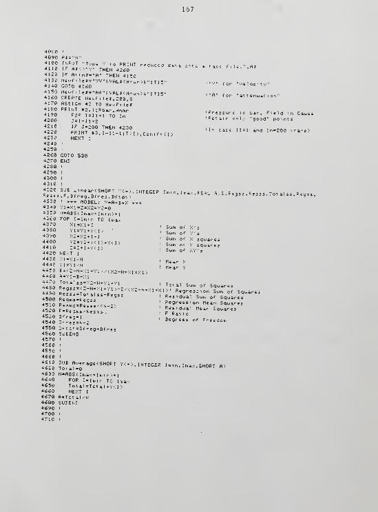
167
4060 i
4090 R*i"N"4100 INPUT "Type V to PRINT reduced dn-, onto a taps f , I
-ft*4110 IF H«0»Y" THEN 4260
P '
4120 IF flttn*=»R« THEN 41504130 Newfile*«''VV"«,Vfi-L*<Nrun>«.»:T15«
i« V " for "uelocitu"4 140 GOTO 4160.tor velocity
4I.-I-. ,-orsTc >i , , , -,„,i»n*» .its i H f 0r "attenuation"tie-o i. kehte Hewf i 1 e* , 200,
8
4170 ASSIGN #3 TO Newfile*4 180 PRINT #3. l;Pbar,Hnmr4190 FOR 1=11+1 TO In
•essure in bar. Field
4200 J = I - 1 1+2! Retain only "good" points
4230 NEXT I
4240 !
4250 !
4260 GOTO 5304270 END4280 <
4290 !
4300 '
4330 ' ••« MODEL: Y«H+E*X ***4340 vi=>:i=2=;:2='v2=e4350 N«flBS<Il»ax-I»in> + l
4360 FOP I = I r., i n TO I r„ a,4370 X1=X1+I . - . „.._„. . ! Sum ot X's4388 i i=Yl+y. i ,
, c * ?,.. r , ! Sum of Y •
s
4390 X2=X2*I+1i e - L
4400 ya-va*v<i».v<»j gj * ^H
mJ! h.x?Ti#v<"
' -•'^2 -
I!!2 ""X1 "NI ".an X4440 Y1=Y1.'N, Me4n y
4450 B=<Z-N*X1*Y1 ) <X2-N*:;i*xi>4460 M=,i-B*::i
llll Joti,s*:Y2-N*Yl*Vl
! Total Su» of Squares
4490 R»;.,. Tn , .-.,.1-L'- .. '" N*xl *xl ' ! Regression Sun of Squares4490 Resss»Totalss-Regss45O0 Regms*Regss
Residual Sun. of Squ a r" -: .
4510 Res»s-Res«'<N-2>! Re!7du*V°M.«*S
"^'^4520 FMegms.Resms-.
,
p**^"* 1 nean Squares
4530 Dfreg»l\ „ . „
4540 D*r«-H-2 degrees of Freedom
4550 Df tot»Dfreg+Dfres4560 SUBEND4570 !
4580 !
4590 i
4600 !
4620 ?ofa? =ra9e<$H ° RT y <*>' INTEGER I '-n. I max, SHORT fl>
4630 N-flBSUaax-Imin . + 1
4640 FOR i = i,„, r, T0 j max4650 Total *Total +Y< I)4660 NEXT I
4670 ft=Tot al N4680 SUBEND4690 i
4700 i
4710 !
168
4720 '
4730 SUE Dplot<Skip,Xlab»,Ylab«, Title*. INTEGER Q, I start , I stop, SHORT X<!4740 COM Fit tnt4750 COM SHORT XI C5> , X2<5> , Yl <5> , Y2<5)4760 SHORT XawCS) , YavC5> , Xdi f <3> , Ydi f <5>4770 PLOTTER IS 13, "GRAPHICS"4780 ' PLOTTER IS "9872A"4790 i OUTPUT 705:"VS10"4800 GRAPHICS4810 i LIMIT 0,385,0,28©4820 ! LOCnTE 20,130,15,954830 LOCATE 20,128,15,854840 SCALE XKQ>,X2<Q>,YKQ>,Y2<Q)
! Defines plot boundaries4850 xdi f (Q^=hes<;;2<;q>-xi <.q^ )
4860 Yd if <Q)=HBS<Y2CQ>-YKQ))4870 Xav<Q) = (Xl<Q> + X2<.G>)>-24888 Yau<Qj=0'l(Q>+Y2(Q)>^24890 GRID Xdif <Q)/-10, Ydif (Q)^10,XKO>, YHQ), 1, 1
4900 i FIXES Xdif (0)^10, Ydi f CQ>/10, XI <;0> , YKQ>, 1 1
4910 FRAME4920 LORG 4
4930 !
4940 !
4950 FOR X=XKG:> TO X2<G> STEP Xdi f (Q>/Sk i p4960 MOVE X,YKQ>-.05*Ydif <Q>4970 ON Q GOTO 4980,4980,4980.50004980 LP.BEL USING "DDD";X4990 GOTO 50105000 LAEEL USING "D.DDD";X501O NEXT X5020 MOVE Xav<Q>,YKQ>-.10*Ydif<O)503O LABEL USING "K" :xiab*5040 i
5O50 !
5060 FOR Y = Y1',Q' TO Y2<Q) STEP Ydif<Q)^Skip5O70 MOVE XKQ>-„08»Xdif <Q>,Y5OS0 ON 9 GOTO 5090.5110,5090,51305090 LABEL USING "DDBDD";Y5100 GOTO 51505110 LFlBEL USING "BD.D";Y5120 GOTO 51505130 IF FtttnS<;"A" THEN GOTO 50905140 LFlBEL USING "D.DD";Y5150 NEXT Y
5160 MOVE XKS)-. 17»Xdif <Q>,Yav(Q)5170 DEG5 ISO LDIR 905190 LABEL USING "K":Ylab#520O LDIR5210 i
5220 '
5230 MOVE X»v<Q>, Y2<G,' + . 05*Ydi f (Cn5240 LABEL USING "K";Title*5250 !
3260 !
5270 Fuf I=Istart TO Istop5280 MOVE X<I),Y<n5290 LFlBEL USING "A"; ". "
530O NEXT I
5310 SUBENIi5320 i
3330 !
5340 !
5350 '
5360 SUB Points' INTEGER Iguess, SHORT :-:<-••
5370 i Poir,»= displays values of data points in the vicinity5330 ! of the input point.5390 FOR I*Iguess-5 TO Iguess*55400 PRINT I .:> I ,
54 10 NEXT I
5420 SUBEND

APPENDIX E
CITED MANUFACTURERS
American Magnetics, Inc., P.O. Box R, Oak Ridge, Tennessee 37820.
Analog Modules, Inc., 400 Sansu Street, Longwood, Florida 32750.
DuPont Company, Plastic Products and Resins Department, Wilmington,Delaware 19898.
Emerson and Cuming, Dielectric Materials Division, Canton, Massachusetts02021.
General Radio Company, 300 Baker Avenue, West Concord, Massachusetts01742.
Hewlett-Packard, Inc., 3495 Deer Creek Road, Palo Alto, California94304.
Intermagnetics General Corporation, Charles Park, P.O. Box 566, Guilder-land, New York 12084.
Jadow and Sons, Inc., New York, New York 10010.
Kepco, Inc., 131-38 Sanford Avenue, Flushing, New York 11352.
Leico Industries, Inc., Fisk Building, 250 West 57th Street, New York,New York 10019.
Linear Research, 5231 Cushman Place, San Diego, California 92110.
Matec, Inc., 60 Montebello Road, Warwick, Rhode Island 02886
Mini-Circuits Laboratories, 2625 East 14th Street, Brooklyn, New York11235.
Nicolet Instrument Corporation, 5225 Verona Road, Madison, Wisconsin53711.
Palomar Engineers, P.O. Box. 455, 1520-G Industrial Avenue, Escondido,California 92025.
Princeton Applied Research Corporation, P.O. Box 2565, Princeton, NewJersey 08540.
169

170
Programmed Test Sources, Inc., 9 Beaverbrook Road, P.O. Box 617, Little-
ton, Massachusetts 01460.
Robertshaw Controls Company, Transportation and Bellows, Marketing
Group, P.O. Box 400, Knoxville, Tennessee 37901.
Vacuum Mstalurgical Company, Ltd., Tokyo, Japan.

REFERENCES
A.I. Ahonen, M. Krusius, and M.A. Paalanen (1976) J. Low Temp. Phys. 25,421.
T.A. Alvesalo, H.K. Collan, M.T. Loponen, O.V. Lounasmaa, and M.C. Veuro(1975), J. Low. Temp. Phys. 19, 1.
T.A. Alvesalo, T. Haavasoja, and M.T. Mannlnen (1981) J. Low Temp. Phys.45, 373.
V. Ambegaokar and D. Mermin (1973) Phys. Rev. Lett._30_, 81.
P.W. Anderson and P. Morel (1961) Phys. Rev. 123 , 1911.
P.W. Anderson and W.F. Brinkman (1973) Phys. Rev. Lett. _30, 1108.
P.W. Anderson and W.F. Brinkman (1978) in The Physics of Liquid andSolid Helium, Part 2 , K.H. Benneman and J.B. Ketterson, eds . , Wiley &
Sons, New York.
E.R. Andrew (1956) Nuclear Magnetic Resonance , Cambrige UniversityPress, London.
0. Avenel, P.M. Berglund, R.G. Gylling, N.E. Phillips, A. Velleseter,and M. Vuorio (1973) Phys. Rev. Lett.
_3J_,76.
0. Avenel, L. Piche, and E. Varoquaux (1981) Physica 107B , 689.
R. Balian and N.R. Werthamer (1963) Phys. Rev. 131 , 1553.
J.L. Bardeen, N. Cooper, and J.R. Schrieffer (1957) Phys. Rev. 108 ,
1175.
R.F. Berg and G.G. Ihas (1983) Cryogenics 23_> 437 «
0. Betbeder-Matibet and P. Nozieres (1969) Ann. Phys._5J_,
392.
N.N. Bogoliubov (1958) Zh. Eksp. Teor. Fiz._34_, 735 (English transla-tion: JETP
_7_ ( 1959) 41, 51).
W.F. Brinkman and P.W. Anderson (1973) Phys. Rev. A _8 , 2732.
W.F. Brinkman, J.W. Serene, and P.W. Anderson (1974) Phys. Rev. A 10,
2386.
171

172
H. Ebisawa and K. Maki (1974) Prog. Theor. Phys ._5J_,
337.
V.J. Emery (1976) J. Low Temp. Phys. _22.» 467.
V.J. Emery (1975) in Quantum Statistics and the Many-Body Problem , S.B.Trickey, W.P. Kirk, J.W. Dufty, eds . , Plenum Publishing, New York.
G. Frossati (1978) J. Physique _39_, 1578.
R.W. Giannetta (1980), Cornell University thesis, unpublished
D.S. Greywall (1983) Phys. Rev. B _27_, 2747.
D.S. Greywall and P. A. Busch (1982) Phys. Rev. Lett. _49, 146.
W.P. Halperin, C.N. Archie, F.B. Rasmussen, T.A. Alvesalo , R.C.Richardson (1976) Phys. Rev. B _13 , 2124.
J. P. Harrison (1979) J. Low Temp Phys . ]H_ y 467.
J.B. Ketterson, P.R. Roach, B.M. Abraham, and P.D. Roach (1975) in
Quantum Statistics and the Many-Body Problem , S.B. Trickey, W.P. Kirk,and J.W. Dufty, eds., Plenum Publishing, New York.
W.P. Kirk and E.D. Adams (1974) Cryogenics 14, 147.
J. A. Konter, R. Hunik, and W.J. Huiskamp (1977) Cryogenics J7, 145.
Y. Kuroda (1975) Prog. Theor. Phys. _53, 349.
L.D. Landau (1956) Zh. Eksp. Teor. Fiz._30, 1058 (English translation:JETP 3, 920)
.
L.D. Landau (1957) Zh. Eksp. Teor. Fiz. _32, 59 (English translation:JETP _5» 101).
L.D. Landau and E.M. Lifshitz (1969) in Statistical Physics , EnglishEdition, Pergamon Press, New York.
D.T. Lawson, H.M. Bozler, and D.M. Lee (1975) in Quantum Statistics andthe Many- Body Problem , S.B. Trickey, W.P. Kirk, and J.W. Dufty, eds.,Plenum Publishing, New York.
D.T. Lawson, W.J. Gully, S. Goldstein, R.C. Richardson, and D.M. Lee(1974) J. Low Temp. Phys. J_5, 169.
D.T. Lawson, W.J. Gully, S. Goldstein, R.C. Richardson, and D.M. Lee(1973) Phys. Rev. Lett._30, 541.
D.M. Lee and R.C. Richardson (1978) in The Physics of Liquid and SolidHelium, Part 2 , K.H. Benneman, J.B. Ketterson, eds., Wiley & Sons, NewYork.
A.J. Leggett (1965) Phys. Rev. A 140, 1869.

173
A.J. Leggett (1972) Phys. Rev. Lett. _29_, 1227.
A.J. Leggett (1973) Phys. Rev. Lett. Jl_> 352.
A.J. Leggett (1974a) Ann. Phys.J35_,
11.
A.J. Leggett (1974b) Prog. Theor. Phys. _51_, 1275.
A.J. Leggett (1975) Rev. Mod. Phys. 47, 331
A.J. Leggett, M.J. Rice (1968) Phys. Rev. Lett. _20_, 536.
K. Levin and O.T. Vails (1977) Phys. Rev. 3 Jo, 4256.
K.. Levin and O.T. Vails (1979) Phys. Rev. B ^0 , 105.
O.V. Lounasnaa (1974) Conterap. Phys.J_5_,
353.
R.H. March and O.G. Symko (1965) Proc. Grenoble Cent. Int. Institute ofRefrigeration, Annexe 2, 57.
N.D. Mermin and G. Stare (1973) Phys. Rev. Lett.J30, 1135.
R.M. Mueller, F. Pobell, and J. Hanssen (1933) Poster presented at theQuantun Fluids and Solids-1983, Sanibel Island, Florida, unpublished.
K..A. Muething (1979) Thesis (Ohio State University, unpublished).
K.A. Muething, G.G. Ihas , and J. Landau (1977) Rev. Sci. Inst. ^8, 906.
Y. Oda, G. Fuji, T. Ono, and H. Nagano (1983) Cryogenics 23_, 139.
D.D. Osheroff and P.W. Anderson (1974) Phys. Rev. Lett. 33_, 686.
D.D. Osheroff, W.J. Gully, R.C. Richardson, and D.M. Lee (1972) Phys.Rev. Lett. 29, 920.
D.D. Osheroff, R.C. Richardson, and D.M. Lee (1972) Phys. Rev. Lett. 28 ,
885.
A. Pal and P. Bhattacharyya (1979) J. Low Temp. Phys.J37_,
379.
D.N. Paulson, R.T. Johnson, and J.C. Wheatley (1973) Phys. Rev. Lett.31, 746.
D.N. Paulson, M. Krusius, and J.C. Wheatley (1977) J. Low Temp. Phys.
26, 1973.
D.N. Paulson and J.C. Wheatley (1978) Phys. Rev. Lett. 41_, 561.
L. Piche, M. Rouff, E. Varoquaux, and 0. Avenel (1982) Phys. Rev. Lett.
_49, 744.
F. Pobell (1982) Physica 109B, 1485.

174
S. Pomeranchuk (1950) Zh. Eksp. Teor. Fiz. _20_, 919.
D. Rainer and J.W. Serene (1976) Phys. Rev. BJ_3, 4745.
R.C. Richardson (1977) Physica 90B , 47.
R.J. Robertson, F. Guillon, and J. P. Harrison (1983) Can. J. Phys. 61 ,
164.
B.V. Rollin (1949) Rep. Progr. Phys. _12, 22.
I. Rudnick (1980) J. Low Temp. Phys. _40_, 287.
V.K. Samalam and J.W. Serene (1978) Phys. Rev. Lett. ^1_ 497.
J. A. Sauls and J.W. Serene (1981) Physica 108B , 1137.
J.W. Serene (1974) Thesis (Cornell University thesis, unpublished).
J.W. Serene and D. Rainer (1979) J. Low Temp. Phys. _34_, 589.
T. Shigi, T. Hata, S. Yamasaki, and T. Kodama, (1983) Quantum Fluids and
Solids-1983 , E.D. Adams and G.G. Ihas, eds . , AIP Conference Proceedings
103, 47.
I.F. Silvera (1980) Rev. Mod. Phys. _52, 393.
G.F. Spencer, P.W. Alexander, and G.G. Ihas (1982) Cryogenics _22_, 167.
G.C. Straty and E.D. Adams (1969) Rev. Sci. Instrum. _40_, 1393.
G.W. Swift and R.E. Packard (1979) Cryogenics _19_, 362.
S. Takagi (1974) Prog. Theor. Phys. _51_> 1993.
S. Takagi (1975) J. Low Temp. Phys. _18_, 309.
D.B. Tanner, G.G. Ihas, and K.A. Meuthing (1977) Rev. Sci. Instrum. 48 ,
610.
L. Tewordt (1974a) J. Low Temp. Phys. _15_, 349.
L. Tewordt (1974b) Z. Phys. 268 , 207.
L. Tewordt, D. Fay, P. Dorre, and D. Einzel (1975) Phys. Rev. B 11,
1914.
L. Tewordt, D. Fay, and N. Schopohl (1978) J. Low Temp. Phys. J30,177.
L. Tewordt and N. Schopohl (1979) J. Low Temp. Phys. 34, 489.
R.A. Webb, R.E. Sager, and J.C. Wheatley (1975a) Phys. Rev. Lett. 35,
615.

175
R.A. Webb, R.E. Sager, and J.C. Wheatley (1975b) Phys. Rev. Lett. 35 ,
1164.
J.C. Wheatley (1975) Rev. Mod. Phys. _47_, 415.
J.C. Wheatley (1978) in Progress in Low Temperature Physics, Vol. 7A ,
D.F. Brewer, ed. , North-Holland, New York.
P. Wolfle (1973) Phys. Rev. Lett. J30, 1169.
P. Wolfle (1975a) Phys. Rev. Lett. 34, 1377.
P. Wolfle (1975b) in Quantum Statistics and the Many-Body Problem , S.B,
Trickey, W.P. Kirk, and J.W. Dufty, eds . , Plenum Publishing, New York.
P. Wolfle (1976a) J. Low Temp. Phys. _22_, 157.
P. Wolfle (1976b) Phys. Rev. B14 , 89.
P. Wolfle (1976c) Phys. Rev. Lett. 37, 1279.
P. Wolfle (1978) in Progress in Low Temperature Physics , Vol. 7A, D.F.
Brewer, ed. North-Holland, New York.
P. Wolfle (1979) Rep. Prog. Phys. _42, 269.
P. Wolfle and V.E. Koch (1978) J. Low Temp. Phys. 30, 61.

BIOGRAPHICAL SKETCH
Robert Frank Berg was born 7 August 1955 in Birmingham, Alabama.
He received a public education in Huntsville, Alabama and later received
the degree of B.S. in Physics with Distinction from the University of
Virginia. His post-graduate education has consisted of two years at
Duke University leading to an M.A. degree followed by four years at the
University of Florida in pursuit of a Ph.D. degree in experimental
physics. His wife of four years is Carol K. Emerson. A member of the
American Physical Society, his published papers and abstracts include
the following titles.
Publications
'gj (He, 2 Sp/gj (XH) in a Low Density Plasma," H.G. Robinson, R.F.
Berg, and C.E. Johnson, Eleventh Annual Meeting of the Division of
Electron and Atomic Physics (1979).
'Cryostat Design for Efficient Use of Liquid Helium," R.F. Gerg and G.G.Ihas, Physica 107B , 595 (1981).
3'Precise Zero Sound Velocity Measurements in the A and Al Phases of He
Near T ," R.F. Berg and G.G. Ihas, in Quantum Fluids and Solids -
1983, eds. E.D. Adams and G.G. Ihas, American Institute of Physics,
p. 353 (1983).
"Direct Comparison of Copper, Silver, and Palladium Heat Exchangers,"R.F. Berg and G.G. Ihas, in Quantum Fluids and Solids - 1983 , eds.E.D. Adams and G.G. Ihas, American Institute of Physics, p. 468,
(1983).
"Simple 100A Current Leads for Low Duty Cycle Use," R.F. Berg and G.G.Ihas, Cryogenics 23, 437 (1983).
176

I certify that I have read this study and that in my opinion itconforms to acceptable standards of scholarly presentation and is fullyadequate, in scope and quality, as a dissertation for the degree ofDoctor of Philisophy.
Y&Jt .
Ck5l
Gary G. Ihas , ChairmanAssociate Professor of Physics
I certify that I have read this study and that in my opinion itconforms to acceptable standards of scholarly presentation and is fullyadequate, in scope and quality, as a dissertation for the degree ofDoctor of Philisophy.
I certify that I have read this study and that in my opinion itconforms to acceptable standards of scholarly presentation and is fullyadequate, in scope and quality, as a dissertation for the degree ofDoctor of Philisophy.
/?
Charles L. BeattyProfessor of Materials Science
and Engineering
I certify that I have read this study and that in my opinion itconforms to acceptable standards of scholarly presentation and is fullyadequate, in scope and quality, as a dissertation for the degree ofDoctor of Philisophy.
rQxA^f KUt^yPradeep KumarAssociate Professor of Physics

I certify that I have read this study and that in my opinion it
conforms to acceptable standards of scholarly presentation and is fullyadequate, in scope and quality, as a dissertation for the degree of
Doctor of Philisophy.
CUfcUsM-Samuel B.
ProfessorTrickeyof Physics
This dissertation was submitted to the Graduate Faculty of the Depart-ment of Physics in the College of Liberal Arts and Sciences and to the
Graduate School, and was accepted as partial fulfillment of the require-
ments for the degree of Doctor of Philosophy.
December 1983Dean for Graduate Studies
and Research