dispersion and dissipation errors of two fully

DISPERSION AND DISSIPATION ERRORS OF TWO

FULLY DISCRETE DISCONTINUOUS GALERKIN

METHODS

HE YANG, FENGYAN LI, AND JIANXIAN QIU

Abstract. The dispersion and dissipation properties of numerical meth-ods are very important in wave simulations. In this paper, such proper-ties are analyzed for Runge-Kutta discontinuous Galerkin methods andLax-Wendroff discontinuous Galerkin methods when solving the linearadvection equation. With the standard analysis, the asymptotic formu-lations are derived analytically for the discrete dispersion relation in thelimit of K = kh → 0 (k is the wavenumber and h is the meshsize) as afunction of the CFL number, and the results are compared quantitativelybetween these two fully discrete numerical methods. For Lax-Wendroffdiscontinuous Galerkin methods, we further introduce an alternative ap-proach which is advantageous in dispersion analysis when the methodsare of arbitrary order of accuracy. Based on the analytical formulationsof the dispersion and dissipation errors, we also investigate the role ofthe spatial and temporal discretizations in the dispersion analysis. Nu-merical experiments are presented to validate some of the theoreticalfindings. This work provides the first analysis for Lax-Wendroff discon-tinuous Galerkin methods.

1. Introduction

In wave simulations, highly accurate numerical methods with good dis-persive and dissipative behaviors are preferred. In this paper, we ana-lyze the dispersion and dissipation errors of two fully discrete high or-der discontinuous Galerkin methods, namely, Runge-Kutta discontinuousGalerkin methods and Lax-Wendroff discontinuous Galerkin methods for aone-dimensional linear advection equation. Discontinuous Galerkin (DG)methods, as one class of finite element methods, use piecewise-defined ap-proximating functions that are discontinuous at mesh interfaces. The meth-ods can be easily designed to have arbitrary order accuracy, with the advan-tages of being compact, free of the inversion of any global mass matrix whensolving time-dependent problems explicitly, suitable for adaptive simulation

Key words and phrases. Discrete dispersion relation; Runge-Kutta discontinuousGalerkin method; Lax-Wendroff discontinuous Galerkin method.

The research of F. Li and H. Yang is partially supported by NSF CAREER awardDMS-0847241 and an Alfred P. Sloan Research Fellowship. The research of J. Qiu ispartially supported by the National Science Foundation of China Grant No. 10931004and ISTCP of China Grant No. 2010DFR00700.

1

2 HE YANG, FENGYAN LI, AND JIANXIAN QIU

and complicated geometry, high parallel efficiency, as well as rich mathe-matical theory in terms of stability and error analysis. The aforementionedproperties of DG methods make them one of the most competitive methodsin many applications which also include various wave equations [10, 11, 2, 4].

DG methods were originally proposed by Reed and Hill [19] to solve thelinear neutron transport equation. The error analysis was established byLesaint and Raviart [15], Johnson and Pitkaranta [14], Richter [20], andPeterson [16]. Motivated by the success for steady state problems, DGmethods were further devised for many time-dependent equations. In [7],Chavent and Salzano constructed a fully discrete scheme using piecewiselinear DG method as spatial discretization and the forward Euler method astime discretization, this method however relies on a very restrictive CFL con-dition for linear stability. Since then there have been many developments intime discretizations, in combination with DG spatial discretizations to getpractically more useful schemes, among which are Runge-Kutta time dis-cretizations and Lax-Wendroff time discretizations. The first DG methodwith Runge-Kutta time discretizations (RKDG) was introduced by Cock-burn and Shu in [8]. The methods were generalized in [9] and are now widelyused in many applications due to their simplicity and being explicit. Someerror analysis was carried out for these fully discrete methods by Zhangand Shu in [24, 25, 26] and also by Zhong and Shu in [27]. DG methodswith the Lax-Wendroff type time discretization (LWDG) were proposed byQiu, Dumbser and Shu [18]. As one-step one-stage high order numericalmethods, when compared with the one-step multi-stage RKDG methods,LWDG methods demonstrate cost efficiency in some applications such astwo-dimensional Euler equations in gas dynamics.

There has been abundant study on the dispersion analysis of many nu-merical methods, with some examples including DG methods [22, 11, 12,2, 21, 4], finite element methods [1, 13, 3], and spectral element methods[23, 5, 6]. Most work was carried out for semi-discrete schemes. In partic-ular, among the dispersion analysis for DG methods, Sherwin [22] studiedthe dispersion relation of the semi-discrete continuous and discontinuousGalerkin methods for the linear advection equation. He obtained analyti-cally the dispersion relation when the discrete spaces involve polynomials ofdegree up to 3, in addition to a numerical study when the polynomial degreeis up to 10. Hu and Atkins [11] examined the semi-discrete DG methods forone- and two-dimensional linear advection equation with the limit kh → 0(k is wavenumber, h is the meshsize). They derived the analytical formu-lations of dispersion and dissipation errors when the polynomials degree isup to 16, and conjectured the formulations for general cases in terms ofsome Pade approximants. This conjecture was proved in [2] by Ainsworth,where he also considered the dispersion relation of hp DG methods in twoother limits. Later, Ainsworth, Monk and Muniz [4] studied the dispersiveand dissipative behavior of semi-discrete DG methods for the acoustic wave

DISPERSION ANALYSIS OF FULLY DISCRETE DG METHODS 3

equation based on either the interior penalty DG methods for the second or-der wave equation or a general DG method applied to the wave equation inits first order form. In terms of fully discrete DG methods, there is much lesswork on the dispersion analysis. Sarmany et al. in [21] considered the DGmethods with Runge-Kutta time discretization for Maxwell equations. Theynumerically evaluated the accuracy order of the dispersion and dissipationerrors of the methods.

In the present work, we focus on the fully discrete DG methods and de-rive analytical formulations of the dispersion and dissipation errors of bothRKDG and LWDG methods in terms of the CFL number for kh ≪ 1, withwhich we carry out comparison between these two methods and further gaininsightful understanding towards the roles of the temporal and spatial dis-cretizations in dispersion and dissipation behavior. In particular, it is shownthat the DG spatial discretizations lead to super-convergence in the disper-sion and dissipation errors compared with the accuracy of the methods inthe L2 norm. This is consistent to the results for the semi-discrete DG meth-ods [11, 2]. However, when Runge-Kutta methods with matching accuracyor the Lax-Wendroff type methods are used as the time discretizations, suchsuper-convergence property is largely lost with the CFL number being or-der one. We believe this is due to the finite difference nature of the timediscretizations. The work in this paper also provides the first (dispersion)analysis for LWDG methods, which have comparable asymptotic dispersionand dissipative behavior as RKDG methods of the same order. For this classof one-step methods, an alternative dispersion analysis is further performed,and it proves to be advantageous for the methods with arbitrary order ofaccuracy.

The remaining of this paper is organized as follows. In section 2, RKDGand LWDG methods are introduced for general one-dimensional conserva-tion laws. In section 3, we first follow the standard dispersion analysis toobtain the analytical discrete dispersion relation of these two methods whensolving the linear advection equation. Such relations are given asymptot-ically in kh ≪ 1 as a function of the CFL number. With these results,comparison is carried out between RKDG and LWDG methods in their dis-persion and dissipation behavior. In section 3, an alternative dispersionanalysis is also given for LWDG methods which can be used to easily an-alyze the methods when they are of any order of accuracy. By examiningthe dispersion and dissipation errors when the CFL number is sufficientlysmall, in section 4, we further gain insight for the roles of the spatial andtemporal discretizations in the dispersion analysis. In section 5, numericalexperiments are presented to validate some of our theoretical findings, whichare followed by concluding remarks in section 6.


2. Formulations of discontinuous Galerkin methods

In this section, we will introduce Runge-Kutta discontinuous Galerkinmethods and Lax-Wendroff discontinuous Galerkin methods for a one-dimensionalscalar conservation law

(2.1) ut + f(u)x = 0, x ∈ [a, b], t > 0.

These are two fully discrete methods which can be of any order of accuracy.Let a = x 1

2

< x 3

2

< · · · < xm+ 1

2

= b be a partition of the computational

domain, with each element denoted as Ij = [xj− 1

2

, xj+ 1

2

], the midpoint of Ij

as xj = (xj− 1

2

+xj+ 1

2

)/2, and the length as hj . We define the approximationspace as

V Nh = v : v|Ij ∈ PN (Ij), j = 1, . . . ,m,

where PN (Ij) is the space of polynomials of degree at most N on Ij. Allfunctions in V N

h are piecewise polynomials, and they are discontinuous at

gridpoints. For any v ∈ V Nh , we also denote v−

j+ 1

2

= limǫ→0− v(xj+ 1

2

+ ǫ)

and v+j− 1

2

= limǫ→0+ v(xj− 1

2

+ ǫ), ∀j.The semi-discrete discontinuous Galerkin method for (2.1) is to look for an

approximated solution uh ∈ V Nh such that for any v ∈ V N

h and j = 1, . . . ,m,there is

(2.2)

∫

Ij

(uh)tvdx−∫

Ij

f(uh)vxdx+ fj+ 1

2

v−j+ 1

2

− fj− 1

2

v+j− 1

2

= 0.

Here fj+ 1

2

(uh) is a numerical flux at xj+ 1

2

that depends on u−h,j+ 1

2

and u+h,j+ 1

2

,

∀j. If we take vjl (x), l = 0, 1, . . . , N as a local basis of V Nh on Ij and repre-

sent the numerical solution as uh(x, t)|Ij =∑N

l=0 Cjl (t)v

jl (x), then equation

(2.2) with j = 1, . . . ,m will become an ODE system for Cjl (t)j,l. If we fur-

ther solve this ODE system by Runge-Kutta time discretizations, this willgive Runge-Kutta discontinuous Galerkin (RKDG) methods for equation(2.1). In section 3, an equivalent formulation of (2.2), namely,

(2.3)

∫

Ij

(uh)tvdx+

∫

Ij

f(uh)xvdx = (f−

j+ 1

2

−fj+ 1

2

)v−j+ 1

2

−(f+j− 1

2

−fj− 1

2

)v+j− 1

2

will be used to derive the discrete dispersion relation.The Lax-Wendroff discontinuous Galerkin (LWDG) method starts with a

Taylor expansion of the solution u in time,

(2.4) u(x, t+∆t) = u(x, t) + ∆tut +∆t2

2utt +

∆t3

6uttt + . . . .

Here we use ∆t to denote the time step. In order to obtain (N + 1)st ordertemporal accuracy, we will keep the first N +1 time derivatives in (2.4) andreplace them with spatial derivatives based on the original partial differential


equation (2.1). For instance, for third order accuracy in time with N = 2,we will replace ut, utt and uttt in (2.4) with

ut = −f(u)x, utt =(

(f ′)2ux)

x, uttt = −

(

3(f ′)2(f ′′)(ux)2 + (f ′)3uxx

)

x,

and approximate u(x, t+∆t) by

u(x, t+∆t) ≈ u(x, t)−∆tFx,

where

(2.5) F = f(u)− ∆t

2(f ′)2ux +

∆t2

6

(

3(f ′)2(f ′′)(ux)2 + (f ′)3uxx

)

.

Note that function F should be FN , and we will drop the subscript N forthe simplicity of notations.

With V Nh as the approximation space, the LWDG method is given as

follows: look for the solution uh ∈ V Nh satisfying

(2.6)∫

Ij

uh(x, t+∆t)vdx =

∫

Ij

uh(x, t)vdx+∆t

∫

Ij

F (uh)vxdx−∆t(Fj+ 1

2

v−j+ 1

2

−Fj− 1

2

v+j− 1

2

),

for any v ∈ V Nh and j = 1, . . . ,m. Here F is a numerical flux, which will

be defined in section 3.2 for a specific f(u) considered in this paper. Theresulting method is formally (N + 1)st order accurate in both space andtime, and it will be termed as LWDG(N+1).

With the same notation of the local basis and the solution representationas for the RKDG method, the LWDG method can be further converted into

an algebraic system for Cjl(tn)j,l,n,

(2.7)N∑

l=0

∫

Ij

vjlvji dx

(

Cjl(tn+1)− Cj

l(tn)

)

= ∆t

∫

Ij

(vji )xFdx−∆t

(

Fj+ 1

2

(vji )−

j+ 1

2

− Fj− 1

2

(vji )+j− 1

2

)

,

for i = 0, 1, . . . , N and j = 1, . . . ,m. Here tnn is for the discrete time,and tn+1 = tn + ∆t. The timestep ∆t can depend on n in practice. Amathematically equivalent form of (2.7) is given as follows,

N∑

l=0

∫

Ij

vjlvji dx

(

Cjl(tn+1)− Cj

l(tn)

)

=−∆t

∫

Ij

Fxvji dx

+∆t

(

(F−

j+ 1

2

− Fj+ 1

2

)(vji )−

j+ 1

2

− (F+j− 1

2

− Fj− 1

2

)(vji )+j− 1

2

)

,(2.8)

and it will be used in next section in the dispersion analysis.

3. Dispersion analysis

In this paper, we focus on the dissipation and dispersion analysis for thefully discrete RKDG methods and LWDG methods defined in section 2 whenthey are applied to the linear advection equation

(3.1) ut + ux = 0, x ∈ (0, 2π], t > 0.


with periodic boundary condition. This corresponds to equation (2.1) withf(u) = u, a = 0, and b = 2π. Without loss of generality, the mesh isassumed to be uniform with hj = h for any j. We choose an orthogonal

local basis, given by the scaled translated Legendre polynomials vjl (x) =√

2l+12 Pl

(

2(x−xj)h

)

. Here Pl(x) with l = 0, . . . , N are the Legendre polyno-

mials on [−1, 1] satisfying Pl(1) = 1. We also define the coefficient vector

Cj = (Cj

0 , Cj1 , . . . , C

jN )T , where Cj

lwith l = 0, 1, . . . , N are the coefficients

in the local expansion of uh.In order to carry out the dispersion analysis, we consider the linear ad-

vection equation (3.1) with an initial condition u(x, 0) = eikx. The exact

solution is given by u(x, t) = ei(kx−ωt) with ω = k. Here k is called thewavenumber, ω is the frequency, and ω = k is the exact dispersion relationfor equation (3.1). Suppose the numerical solution of a method is of the sameform, namely, uh(x, t) = ei(kx−ωt) = eωitei(kx−ωrt). When ωi = ℑ(ω) < 0,the scheme is dissipative. And ωr = ℜ(ω) 6= k gives a dispersive solution.By taking into account how fine the mesh is with respect to the wavenumberk, we further define K = kh and Ω = Ωr+ iΩi with Ωr = ωrh and Ωi = ωih,then the exact dispersion relation can be expressed as Ωr = K and Ωi = 0.Our goal is to estimate the dispersion error Ωr −K and the dissipation er-ror Ωi of the RKDG and LWDG methods with respect to the CFL numberν = ∆t

hfor K ≪ 1. In this paper, all reference values of the CFL number to

ensure the linear stability of the scheme come from literature.

3.1. Analysis of RKDG methods. To allow information propagate sta-bly, we use an upwind numerical flux for the semi-discrete DG method in(2.3) when it is applied to (3.1). That is, fj+ 1

2

= uh,j+ 1

2

= u−h,j+ 1

2

, ∀j. Thenthe method becomes∫

Ij

uh,tvdx+

∫

Ij

uh,xvdx = (u−h,j+ 1

2

− uh,j+ 1

2

)v−j+ 1

2

− (u+h,j− 1

2

− uh,j− 1

2

)v+j− 1

2

= −(u+h,j− 1

2

− u−h,j− 1

2

)v+j− 1

2

(3.2)

for j = 1, . . . ,m, and it can be further written into a matrix form

(3.3)dCj

dt=

2

h

(

−(D0 +G+0 )C

j +G−

0 Cj−1)

,

once the solution representation is taken in terms of the local basis. Herethe (s, l)-th entry of the matrices D0, G

−

0 , G+0 is defined as

D0(s, l) =

∫

Ij

vjs∂vj

l

∂xdx,G−

0 (s, l) = (vjsvj−1l )|x

j− 12

, G+0 (s, l) = (vjsv

jl )|xj− 1

2

,

respectively. It is easy to see that these matrices are independent of indexj, therefore the notations D0, G

+0 and G−

0 will not lead to any confusion.


With U = −(D0 + G+0 ), L = G−

0 , we rewrite equation (3.3) with j =1, . . . ,m into an ODE system

(3.4)

dC1

dtdC2

dt......

dCm

dt

=2

h

U 0 . . . 0 LL U

. . .. . .. . .

. . .

L U

C1

C2

...

...C

m

which can also be compactly denoted as dCdt

= AC, with A being the coef-

ficient matrix and C = ((C1)T , . . . , (Cm)T )T . We then solve this ODE sys-tem from time t to t+∆t by Runge-Kutta (RK) methods. For instance, the2-stage 2nd order RK method gives C(t+∆t) =

(

I +∆tA+ 12(∆tA)2

)

C(t),

and the 3-stage 3rd order RKmethod givesC(t+∆t) =(

I +∆tA+ 12 (∆tA)2 + 1

6(∆tA)3)

C(t).In this paper, we will use RKDG(N+1) to denote the fully discrete schemewhich uses the upwind DG method in (3.4) (also see (3.2)) with the discretespace V N

h as the spatial discretization, and the (N+1)-stage (N+1)st orderRK method as the time discretization.

3.1.1. RKDG2 with N = 1. With a simple derivation, RKDG2 can be writ-ten as

Cj(t+∆t) = 2ν2L2

Cj−2(t) +

(

2νL+ 2ν2(LU + UL))

Cj−1(t)

+(

I + 2νU + 2ν2U2)

Cj(t).(3.5)

Let Cj(t) = α exp(i(kxj − ωt)), with α being a nonzero constant vector oflength N +1. We substitute it into equation (3.5) and obtain an eigenvalueproblem

(3.6) (e−iω∆tI −M)α = 0,

where

(3.7) M = 2ν2L2e−2ikh+(

2νL+ 2ν2(LU + UL))

e−ikh+I+2νU+2ν2U2.

This 2× 2 matrix M has two eigenvalues, and if we denote one as λ, then

(3.8)

Ωr = − 1νarctan

(

ℑ(λ)ℜ(λ)

)

,

Ωi =12ν ln

(

(ℜ(λ))2 + (ℑ(λ))2)

.

For K = kh ≪ 1, there is only one eigenvalue of M, satisfying Ωr ∼ K asK → 0, which is physically relevant and is said to be consistent. Based onthe consistent eigenvalue of M in (3.7), we obtain

(3.9)

Ωr = K + 16ν

2K3 +(

1270 − 1

20ν4)

K5 +O(K7),Ωi =

(

− 172 +

18ν

3)

K4 +(

1648 − 1

144ν2)

K6 +O(K8).

This indicates that the dispersion error Ωr−K is of third order accuracy withrespect to K ≪ 1, and the dissipation error Ωi is of fourth order accuracy.When k = O(1), this is equivalent to say that the dispersion error ωr − k


is of second order accuracy and the dissipation error ωi is of third orderaccuracy in h ≪ 1.

It seems that a careful selection of the CFL number ν may lead to − 172 +

18ν

3 = 0 and therefore give higher accuracy in dissipation error. However, tomake this happen, one must choose ν ≈ 0.4807, which is beyond the linearstability limit of RKDG2, ν ≤ 1

3 . In other words, the result in (3.9) is sharp,and no higher order accuracy can be achieved for either the dissipative erroror the dispersive error by simply changing the constant ν. (Later in section4, a different scenario is discussed when ν is allowed to depend on K.) Notethat the dominating error is from dispersion, and the coefficient of its leadingterm is an increasing function of ν and it is always positive. Therefore asmaller CFL number leads to a smaller dispersion error. On the other hand,since | − 1

72 + 18ν

3| increases as ν → 0+, a smaller CFL number leads to alarger dissipation error.

For a given wavenumber k, by making use of the asymptotic formulain (3.9), we can estimate the total dispersion and dissipation errors of theRKDG2 solution up to a given time T for sufficiently small mesh size h. Tobe more concrete, assume the numerical solution is(3.10)

uh(x, T ) = ei(kx−ωT ) = eℑ(ω)T ei(kx−ℜ(ω)T ) = eΩiTh ei(K−Ωr)

Th ei(kx−kT ),

then eΩiTh ∼ e(−

1

72+ 1

8ν3)K4 T

h measures the total dissipation error, and ei(K−Ωr)Th ∼

e−1

6iν2K3 T

h measures the total dispersion error up to time T . These ap-proximations can provide useful guidance for one to control errors in wavesimulations.

3.1.2. RKDG3 with N = 2. Following the similar procedure for RKDG2, weobtain an eigenvalue problem (3.6) for the dispersion analysis of RKDG3,where M = A1e

−3ikh +A2e−2ikh +A3e

−ikh +A4 with

A1 =4

3ν3L3,

A2 =4

3ν3(L2U + LUL+ UL2) + 2ν2L2,

A3 =4

3ν3(LU2 + ULU + U2L) + 2ν2(LU + UL) + 2νL,

A4 = I +4

3ν3U3 + 2ν2U2 + 2νU.

When we use symbolic computation software MAPLE to obtain the con-sistent eigenvalues of M, in order to simplify the lengthy result and getan analytical form of the leading term, the following nontrivial equality isidentified and proves to be crucial,

52 + 72ν − 3240ν2 + 8260ν3 + 6360ν4 − 11568ν5 − 33408

+√17(20 − 120ν + 120ν2 − 420ν3 + 3720ν4 − 3600ν5 − 8000ν6)


= (1 + 7ν − 24ν2 +√17− 3

√17ν − 4

√17ν2)3.

With this, the consistent eigenvalue of M is simply given by

λ = 1− iνK − 1

2ν2K2 + i

1

6ν3K3 +O(K6),

and we further obtain from (3.8)

(3.11)

Ωr = K + 130ν

4K5 + ( 142000 − 1

252ν6)K7 +O(K8),

Ωi = − 124ν

3K4 + ( 172ν

5 − 17200 )K

6 +O(K8).

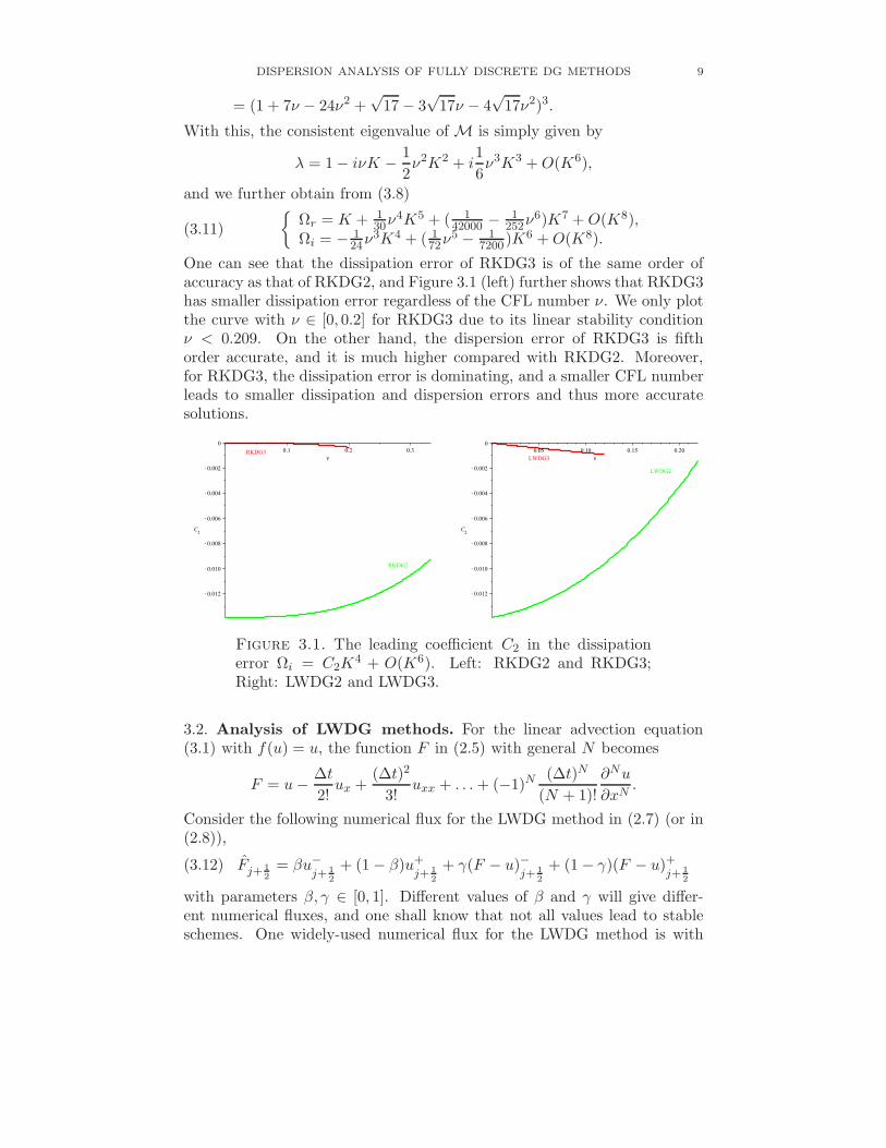
One can see that the dissipation error of RKDG3 is of the same order ofaccuracy as that of RKDG2, and Figure 3.1 (left) further shows that RKDG3has smaller dissipation error regardless of the CFL number ν. We only plotthe curve with ν ∈ [0, 0.2] for RKDG3 due to its linear stability conditionν < 0.209. On the other hand, the dispersion error of RKDG3 is fifthorder accurate, and it is much higher compared with RKDG2. Moreover,for RKDG3, the dissipation error is dominating, and a smaller CFL numberleads to smaller dissipation and dispersion errors and thus more accuratesolutions.

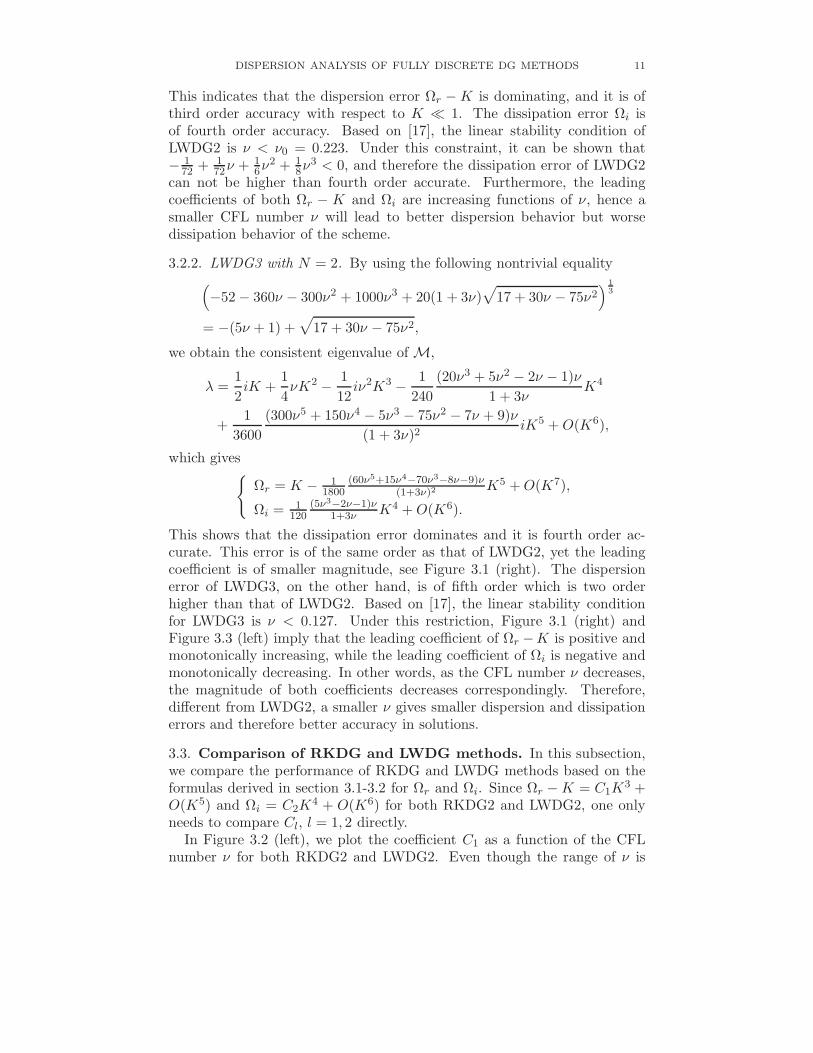
Figure 3.1. The leading coefficient C2 in the dissipationerror Ωi = C2K

4 + O(K6). Left: RKDG2 and RKDG3;Right: LWDG2 and LWDG3.

3.2. Analysis of LWDG methods. For the linear advection equation(3.1) with f(u) = u, the function F in (2.5) with general N becomes

F = u− ∆t

2!ux +

(∆t)2

3!uxx + . . .+ (−1)N

(∆t)N

(N + 1)!

∂Nu

∂xN.

Consider the following numerical flux for the LWDG method in (2.7) (or in(2.8)),

(3.12) Fj+ 1

2

= βu−j+ 1

2

+ (1− β)u+j+ 1

2

+ γ(F − u)−j+ 1

2

+ (1− γ)(F − u)+j+ 1

2

with parameters β, γ ∈ [0, 1]. Different values of β and γ will give differ-ent numerical fluxes, and one shall know that not all values lead to stableschemes. One widely-used numerical flux for the LWDG method is with


β = 1, γ = 12 . In this subsection, we will focus on the dispersion analysis of

the LWDG method with this numerical flux.In order to derive the compact matrix form of the LWDG method, we

define matrices E−, E+, G−, G+ and D, which all depend on N and havethe (s, l)-th entries given as follows.

E−(s, l) =

(

(1− β)vjsvjl+ (1− γ)(−∆t

2!vjs

∂vjl∂x

+ . . .+ (−1)N(∆t)N

(N + 1)!vjs

∂Nvjl∂xN

)

)

xj+1

2

,

(3.13)

E+(s, l) =

(

(1− β)vjsvj+1l + (1− γ)(−∆t

2!vjs

∂vj+1l

∂x+ . . . + (−1)N

(∆t)N

(N + 1)!vjs

∂Nvj+1l

∂xN)

)

xj+1

2

,

G−(s, l) =

(

βvjsvj−1l + γ(−∆t

2!vjs

∂vj−1l

∂x+ . . .+ (−1)N

(∆t)N

(N + 1)!vjs

∂Nvj−1l

∂xN)

)

xj− 1

2

,

G+(s, l) =

(

βvjsvjl + γ(−∆t

2!vjs

∂vjl

∂x+ . . .+ (−1)N

(∆t)N

(N + 1)!vjs

∂Nvjl

∂xN)

)

xj− 1

2

,

D(s, l) =

∫

Ij

vjs∂vj

l

∂xdx− ∆t

2!

∫

Ij

vjs∂2vj

l

∂x2dx+ . . . + (−1)N

(∆t)N−1

N !

∫

Ij

vjs∂Nvj

l

∂xNdx.

Using these matrices, the LWDG method in (2.8) can be rewritten as(3.14)1

2ν

(

Cj(t+∆t)−C

j(t))

= (E−−G+−D)Cj(t)+G−C

j−1(t)−E+C

j+1(t).

To carry out the dispersion analysis, we take the ansatzCj(t) = α exp(i(kxj−ωt)) in (3.14), with α being a nonzero constant vector, and obtain the fol-lowing eigenvalue problem

(3.15)

(

e−iω∆t − 1

2νI +M

)

α = 0,

where M = (D +G+ − E−) + E+eikh −G−e−ikh. If one of the eigenvalues

of M is denoted as λ and let λ = 1− 2νλ, we will have

(3.16)

Ωr = ℜ(ω)h = − 1νarctan

(

ℑ(λ)

ℜ(λ)

)

,

Ωi = ℑ(ω)h = 12ν ln

(

(ℜ(λ))2 + (ℑ(λ))2)

.

3.2.1. LWDG2 with N = 1. For LWDG2, the physically relevant dispersionrelation is given as

Ωr = K +(

112ν + 1

6ν2)

K3 +O(K5),Ωi =

(

− 172 + 1

72ν + 16ν

2 + 18ν

3)

K4 +O(K6).


This indicates that the dispersion error Ωr −K is dominating, and it is ofthird order accuracy with respect to K ≪ 1. The dissipation error Ωi isof fourth order accuracy. Based on [17], the linear stability condition ofLWDG2 is ν < ν0 = 0.223. Under this constraint, it can be shown that− 1

72 + 172ν + 1

6ν2 + 1

8ν3 < 0, and therefore the dissipation error of LWDG2

can not be higher than fourth order accurate. Furthermore, the leadingcoefficients of both Ωr − K and Ωi are increasing functions of ν, hence asmaller CFL number ν will lead to better dispersion behavior but worsedissipation behavior of the scheme.

3.2.2. LWDG3 with N = 2. By using the following nontrivial equality(

−52− 360ν − 300ν2 + 1000ν3 + 20(1 + 3ν)√

17 + 30ν − 75ν2) 1

3

= −(5ν + 1) +√

17 + 30ν − 75ν2,

we obtain the consistent eigenvalue of M,

λ =1

2iK +

1

4νK2 − 1

12iν2K3 − 1

240

(20ν3 + 5ν2 − 2ν − 1)ν

1 + 3νK4

+1

3600

(300ν5 + 150ν4 − 5ν3 − 75ν2 − 7ν + 9)ν

(1 + 3ν)2iK5 +O(K6),

which gives

Ωr = K − 11800

(60ν5+15ν4−70ν3−8ν−9)ν(1+3ν)2

K5 +O(K7),

Ωi =1

120(5ν3−2ν−1)ν

1+3ν K4 +O(K6).

This shows that the dissipation error dominates and it is fourth order ac-curate. This error is of the same order as that of LWDG2, yet the leadingcoefficient is of smaller magnitude, see Figure 3.1 (right). The dispersionerror of LWDG3, on the other hand, is of fifth order which is two orderhigher than that of LWDG2. Based on [17], the linear stability conditionfor LWDG3 is ν < 0.127. Under this restriction, Figure 3.1 (right) andFigure 3.3 (left) imply that the leading coefficient of Ωr −K is positive andmonotonically increasing, while the leading coefficient of Ωi is negative andmonotonically decreasing. In other words, as the CFL number ν decreases,the magnitude of both coefficients decreases correspondingly. Therefore,different from LWDG2, a smaller ν gives smaller dispersion and dissipationerrors and therefore better accuracy in solutions.

3.3. Comparison of RKDG and LWDG methods. In this subsection,we compare the performance of RKDG and LWDG methods based on theformulas derived in section 3.1-3.2 for Ωr and Ωi. Since Ωr −K = C1K

3 +O(K5) and Ωi = C2K

4 + O(K6) for both RKDG2 and LWDG2, one onlyneeds to compare Cl, l = 1, 2 directly.

In Figure 3.2 (left), we plot the coefficient C1 as a function of the CFLnumber ν for both RKDG2 and LWDG2. Even though the range of ν is


taken as (0, 13 ), the curve for LWDG2 is valid only for ν ∈ (0, 0.223) dueto the linear stability restriction. Both curves are monotonically increasing,and for the same ν, RKDG2 has smaller dispersion error than LWDG2.In addition, with a widely used CFL number, namely, 1

3 for RKDG2 and0.22 for LWDG2, we have C1 = 1.85E-2 for RKDG2 and C1 = 2.33E-2 forLWDG2. Therefore, even in this case, RKDG2 still has better performancein dispersion behavior. Figure 3.2 (right) gives the curves of the coefficientC2 of RKDG2 and LWDG2, and both are increasing functions of ν. Withinthe stability range of LWDG2, both functions are negative. For a fixed ν inthis range, LWDG2 has better dissipation behavior than RKDG2. This isalso true if ν = 1

3 is taken for RKDG2 and ν = 0.22 is for LWDG2.

Figure 3.2. Left: The leading coefficient C1 in the disper-sion error Ωr = K+C1K

3+O(K5) for RKDG2 and LWDG2.Right: The leading coefficient C2 in the dissipation errorΩi = C2K

4 +O(K6) for RKDG2 and LWDG2.

For RKDG3 and LWDG3 with N = 2, there are Ωr−K = C1K5+O(K7)

and Ωi = C2K4+O(K6). Figure 3.3 shows that both C1 and C2 for RKDG3

are of much smaller magnitude than those for LWDG3, therefore RKDG3has better dispersion and dissipation behavior with more accurate numericalsolutions than LWDG3. Note that for N = 1, 2, both RKDG and LWDGmethods have positive C1. This implies a phase lead, which is confirmed bynumerical experiments in section 5 (see Table 5.1 and Table 5.3).

When N ≥ 3, for the eigenvalue problems arising in the dispersion anal-ysis of RKDG(N+1) and LWDG(N+1), we can no longer obtain a compactasymptotic formula of the consistent eigenvalue as a function of the CFLnumber ν with respect to K ≪ 1, hence we will not include any discussionfor these cases. One can surely numerically evaluate the dispersion relationwith a given ν for larger N as in [21] by following the analysis in sections3.1 and 3.2.

3.4. An alternative analysis for LWDG methods: the fixed-ω method.

The dispersion analysis in sections 3.1-3.2 is a standard approach, whichsolves the eigenvalue problem (3.6) or (3.15) for the frequency ω in terms


Figure 3.3. Left: The leading coefficient C1 in the disper-sion error Ωr = K+C1K

5+O(K7) for RKDG3 and LWDG3.Right: The leading coefficient C2 in the dissipation errorΩi = C2K

4 +O(K6) for RKDG3 and LWDG3.

of the wavenumber k. The advantage of this approach is the clearness ofits physical meaning, since the wavenumber k is usually given in the initialcondition. However, when we use the (N + 1)st order RKDG or LWDGmethod, in order to obtain the formulation of e−iω∆t in terms of k, a poly-nomial equation of degree N +1 needs to be solved, and this becomes morecomplicated for larger N . On the other hand, when solving the eigenvalueproblem (3.15) for the LWDG method by computing the determinant of thecoefficient matrix, if one solves the wavenumber in terms of the frequency,the eigenvalue problem will be much simpler. This is stated more rigorouslyin the next Theorem.

Theorem 3.1. Suppose h > 0, N ∈ N and β, γ ∈ [0, 1]. Consider the

(N + 1)st order LWDG method with the numerical flux defined in (3.12),then the discrete dispersion relation is determined by the consistent solution

of the eigenvalue problem (3.15). Moreover, (i) For N = 0, the eigenvalue

problem is a quadratic equation in terms of ξ = eikh when 0 < β < 1, and it

is linear when β = 0 or β = 1. (ii) For N ≥ 1, when (β− 1)2 +(γ− 1)2 6= 0and β2 + γ2 6= 0, the eigenvalue problem is a quadratic equation in terms of

ξ = eikh. When β = γ = 1 or β = γ = 0, the eigenvalue problem turns to a

linear polynomial equation.

Proof. The eigenvalue problem (3.15) has nontrivial solutions if and only ifthe determinant of the coefficient matrix M is equal to zero. The conclusionfor N = 0 is straightforward, as all the involved matrices are scalar, we hereonly focus on the cases with N ≥ 1. When β and γ are not equal to 0or 1 at the same time, it is easy to show that matrices E+ and G− are ofrank 1. By the properties of determinant under row or column operations,the determinant of the matrix is of the form δ1 + δ2e

ikh + δ3e−ikh, where

δi, i = 1, 2, 3 are constants. Therefore the solution of the eigenvalue problem


(3.15) is the root of δ2ξ2 + δ1ξ + δ3 = 0 with ξ = eikh. When β = γ = 1, we

have E+ = 0 based on its definition in (3.13). In this case, the determinantcan be reduced to δ1 + δ3e

−ikh, thus the problem leads to a first orderequation δ1ξ+δ3 = 0. Similarly, when β = γ = 0, we have G− = 0 in (3.15).Following the same discussion, we can also obtain that the problem leads toa linear polynomial equation.

Given the frequency ω, u(x, t) = ei(kx−ωt) is the exact solution for (3.1)with the wavenumber k = ω. Assume the numerical solution of the LWDGmethods is of the same form, namely, uh(x, t) = ei(kx−ωt). Following [2],

we define the relative error ρN = eikh−eikh

eikh. Note that ρN ≈ i(k − k)h with

K = kh ≪ 1, and it measures the difference between the exact and thediscrete wavenumbers multiplied by the mesh parameter h and thereforegives the dispersion error of the schemes. Theorem 3.1 implies that with thefixed-ω method, one can obtain the analytical formulation of the consistenteigenvalue for any N and therefore the discrete dispersion relation for ar-bitrary order LWDG methods. This is a huge advantage over the standardapproach. The fixed-ω approach was used in [2] to analyze the dispersionproperty for the semi-discrete DG methods of any order of accuracy.

For the commonly-used numerical flux given by (3.12) with β = 1, γ = 12 ,

we can easily compute the asymptotic formulation of the relative error ρN ,and the results for N = 0, 1, . . . , 4 are given as follows.

ρ0 =

(

1

2− ν

2

)

K2 + i

(

1

3− ν

2+

1

6ν2)

K3 +O(K4)

ρ1 = i

(

1

12ν +

1

6ν2)

K3 +

(

1

72− 1

72ν − 1

6ν2 − 1

8ν3)

K4 +O(K5)

ρ2 = − 1

120

ν(5ν3 − 2ν − 1)

3ν + 1K4 − i

1800

(60ν5 + 15ν4 − 70ν3 − 8ν − 9)ν

(3ν + 1)2K5 +O(K6)

ρ3 = − i

5040

(35ν5 − 43ν3 + 20ν + 3)ν

5ν2 + 1K5

+1

70560

(2975ν6 + 175ν5 − 4105ν4 − 470ν3 + 830ν2 + 316ν + 24)ν

(5ν2 + 1)2K6 +O(K7)

ρ4 =1

90720

(147ν7 − 455ν5 + 343ν3 − 20ν − 3)ν

10ν + 1K6

− i

816480

ξ

(1 + 20ν + 100ν2)K7 +O(K8)

where ξ = 9261ν12 − 45570ν10 − 1323ν9 + 56999ν8 + 855ν7 − 22842ν6 +189ν5 + 2574ν4 + 165ν3 + 73ν2 + 15ν. For the linear advection equation(3.1), one can also consider the fully upwind numerical flux, namely (3.12)with β = γ = 1. When N = 0, ρ0 has the same formulation as above. And


ρN , with N = 1, . . . , 4, are given as follows.

ρ1 =i

12

(

ν − ν2)

K3 +

(

1

72− 1

18ν +

1

24ν2)

K4 +O(K5)

ρ2 =1

120

(

ν − ν2)

K4 + i

(

1

180ν4 +

1

200ν − 19

1800ν2)

K5 +O(K6)

ρ3 = i

(

− 1

504ν2 − 1

720ν4 − 1

1680ν

)

K5

+

(

1

2940ν − 59

70560ν2 +

1

2016ν4)

K6 +O(K7)

ρ4 =

(

1

9072ν2 − 1

30240ν − 1

12960ν4)

K6

+ i

(

11

116640ν2 − 1

54432ν − 1

3645ν4 +

1

5040ν6)

K7 +O(K8)

Based on the formulations of ρN for the LWDG methods using the nu-merical flux with β = 1, and γ = 1

2 or 1, the following pattern can beobserved,

(3.17) ρN =

C2KN+3 + iC1K

N+2 +O(KN+4), if N is odd,C1K

N+2 + iC2KN+3 +O(KN+4), if N is even,

where C1, C2 are two real constants dependent of the CFL number ν and N .These formulas show that the relative error ρN is of order N+2 in K ≪ 1 forthe (N +1)st order LWDG methods. Here C1 or iC1 denotes the coefficientof the leading order term. The formulas can be used to further study therelative error. For instance, in Figure 3.4, ln(|C1|) is plotted as a functionof ν for the method with β = 1 and γ = 1

2 . One can conclude that when Nincreases, not only ρN will be of higher order accuracy, the magnitude of theleading coefficient |C1| will also decrease significantly. Since ln(|C1|) → −∞as ν → 0, we only plot ln(|C1|) for ν from 10−5 to 0.22.

Remark 3.2. (1) Though a similar result as in theorem 3.1 holds for thesemi-discrete DG method in (3.2) (see [2]), it does not hold for fully discreteRKDG methods. It can be shown that the eigenvalue problem in the disper-sion analysis for the RKDG3 method leads to a cubic polynomial equationin terms of eikh.

(2) −ℜ(ρN ) ≈ −ℑ(kh) and ℑ(ρN ) ≈ ℜ(kh− kh) measure the dissipationand dispersion errors of LWDG methods, respectively. This is consistentto the observation that for LWDG(N+1) with N = 1, 2, −ℜ(ρN ) is of thesame order of accuracy as Ωi, and ℑ(ρN ) is of the same order of accuracyas Ωr −K.

One natural question is, can we design LWDG methods with a higherorder relative error ρN if the parameters β and γ take some special valuesin the numerical flux (3.12)? When N = 0, the numerical flux is given by


Figure 3.4. ln(|C1|), with C1 defined in (3.17), for the(N + 1)st order LWDG method using the numerical flux(3.12) with β = 1 and γ = 1

2 , N = 1, . . . , 4. The solid,dot, long-dash and space-dash lines represent the case whenN = 1, 2, 3, 4 respectively.

F = βu− + (1− β)u+, and the relative error is given as,

ρ0 = (β − 1 + ν

2)K2 +

i

6(12β2 − 6νβ − 12β + ν2 + 3ν + 2)K3 +O(K4).

One can see that for general value of β, there is ρ0 = O(K2) and this isconsistent to our previous observation. Yet when β and the CFL numberν are properly related, namely, β = 1+ν

2 , ρ0 will be one order higher with

ρ0 = O(K3). In this case, the numerical flux becomes F = 1+ν2 u− + 1−ν

2 u+

which is upwind-biased. Numerical experiments with ν = 0.2, 0.4, 0.6, 0.8also indicates that the resulting method is stable. The success of the LWDG1withN = 0 unfortunately can not be carried over to generalN . For example,when N = 1 with F = βu− + (1− β)u+ − ∆t

2 (γu−x + (1− γ)u+x ), in order to

improve the accuracy order of ρ1 from O(K3) to O(K4), one needs β = 12

and γ = 12 + 1

6ν . Note that ν appears in the denominator of γ which growsunboundedly when ν approaches 0. Numerical tests show that the resultingmethod, though formally with higher order relative error ρ1, is unstable.

4. The role of the spatial and the temporal discretizations

In section 3, we have derived the analytical formulations of the leadingterms of the dispersion and dissipation errors, Ωr − K and Ωi, of RKDGand LWDG methods, as well as the relative error ρN for LWDG methods,as a function of the CFL number ν. The analysis is carried out by assumingν is a constant. In this section, we will further discuss these results whenν can depend on K and therefore can be chosen to be “smaller”, with thegoal to understand the role of the spatial and the temporal discretization inthe dispersion analysis for the fully discrete methods.


We start with RKDG methods. In section 3.1, we obtain for RKDG2 thedispersive error Ωr −K = 1

6ν2K3 + ( 1

270 − 120ν

4)K5 +O(K7) which is third

order accurate. Note that limν→016ν

2 = 0 and limν→01

270 − 120ν

4 = 1270 . If

ν is taken to be “smaller”, in particular with ν = O(Kr) and r ≥ 1, thenΩr − K = O(K5) and it is two order more accurate. On the other hand,smaller ν will not change the overall fourth order accuracy of the dissipativeerror Ωi = (− 1

72 + 18ν

3)K4 + O(K6) = O(K4). Since the properties of thefully discrete schemes with sufficiently small CFL numbers are determinedonly by spatial discretizations, one can conclude that the second order DGspatial discretization contributes to RKDG2 with Ωr − K = O(K5) andΩi = O(K4), yet the second order Runge-Kutta time discretization reducesthe order of the dispersive error by two while keeping the dissipative errorunchanged. Similarly, for RKDG3, from the dispersion analysis given in(3.11), and with the sufficiently small CFL number, namely ν = O(Kr) andr ≥ 2

3 , the dispersive error becomes Ωr − K = O(K7) and the dissipative

error is Ωi = O(K6), and these can be attributed to the third order DGspatial discretization, while the third order Runge-Kutta time discretizationreduces the order of both dispersive and dissipative errors by two, renderingΩr −K = O(K5) and Ωi = O(K4).

Next we consider LWDG methods. For LWDG2, the dispersion and dis-sipation errors are given as

Ωr = K + ( 112ν + 1

6ν2)K3 + ( 1

270 + 5432ν − 11

144ν2 − 1

8ν3 − 1

20ν4)K5 +O(K7),

Ωi = (− 172 + 1

72ν + 16ν

2 + 18ν

3)K4 + ( 1648 + 17

2592ν − 29864ν

2 − 796ν

3 − 120ν

4)K6 +O(K8).

With ν = O(Kr) and r ≥ 2, we have Ωr − K = O(K5) and Ωi = O(K4),and they are determined by the spatial discretization in LWDG2, whilethe time discretization in LWDG2 is responsible for Ωr −K = O(K3) andΩi = O(K4). For LWDG3, there is

Ωr = K − 11800

(60ν5+15ν4−70ν3−8ν−9)ν(1+3ν)2

K5 + ξ

3780000(1+3ν4)K7 +O(K8),

Ωi =1

120(5ν3−2ν−1)ν

1+3ν K4−1

360001500ν8+750ν7−2150ν6−3075ν5+830ν4+1950ν3+439ν2−33ν+5

(1+3ν)3K6 +O(K8),

with ξ = 45000ν10 +33750ν9 − 148500ν8 +27375ν7 − 94100ν6 − 142275ν5 +97415ν4 + 129000ν3 + 24327ν2 − 2994ν + 90. Then with ν = O(Kr) andr ≥ 2, the dispersion and dissipation errors of LWDG3 are Ωr−K = O(K7)and Ωi = O(K6), and they are attributed to the spatial discretization ofLWDG3, while its temporal discretization is responsible for the two orderlower dispersive error Ωr−K = O(K5) and the dissipative error Ωi = O(K4)of the fully discrete LWDG3. Compared with RKDG(N+1), N = 1 or 2, inorder to extract the contribution of the spatial discretization, one needs touse relatively smaller ν and therefore smaller time-step ∆t in LWDG(N+1).

Based on the analysis given so far, one can see that with sufficientlysmall CFL numbers, both RKDG and LWDG methods have a (2N + 3)rd

order dispersive error Ωr − K, and a (2N + 2)nd order dissipative error


Ωi where N = 1, 2. Since these orders of accuracy are higher than theexpected (N + 1)st order of accuracy of the methods in the L2 norm, thespatial discretizations of both RKDG and LWDG methods lead to super-

convergence in dispersion and dissipation errors. When the wavenumber k isgiven, by taking into account the factor h in Ωr and Ωi, we also say that thedispersive error ωr−k due to the spatial discretization is (N+1)st order moreaccurate and the dissipative error ωi is N th order more accurate than theL2 errors of the RKDG or LWDG numerical solutions. On the other hand,the temporal discretization reduces the super-convergence in the dispersiveerror when N = 2, while completely eliminating the super-convergence inthe dispersive error when N = 1 and in the dissipative error when N = 2.

Finally, we turn our discussion to the relative error ρN obtained for theLWDG methods in section 3.4. With the similar analysis as for Ωr −K andΩi, based on ρN , N = 0, . . . , 5 of the LWDG methods using the numericalflux (3.12) with β = 1 and γ = 1

2 , and with the CFL number ν = O(Kr)and r ≥ N + 2 for K ≪ 1, we obtain(4.1)

ρN =1

2

(

N !

(2N + 1)!

)2

K2N+2+i

(

N !

(2N + 1)!

)2 N + 1

(2N + 1)(2N + 3)K2N+3+O(K2N+4).

We conjecture that (4.1) also holds for general N . One can see that ρN forLWDG methods is of (2N +2)nd order accuracy if the influence of time dis-cretizations can be neglected, and this is a super-convergent property, similaras previously discussed for Ωr −K and Ωi. In [2], the asymptotic formula-tions of the relative error ρN was mathematical proved for the semi-discreteupwind DG method in (3.2) with any N . In this case ρN is completelydetermined by the spatial DG discretizations. Although LWDG methodsdo not have a semi-discrete version when ∆t → 0, one can still compareρN in (4.1) and that in [2]. Indeed, the formula of ρN in (4.1) is identicalto that of the semi-discrete upwind DG method in (3.2). Hence the spatialdiscretization of LWDG methods contributes to ρN in a similar way as thatof the semi-discrete DG methods. The results in section 3.4 show that ρN isof order (N +2) with ν = O(1), indicating that the time discretization elim-

inates the super-convergence in ρN . (Recall that ρN ≈ i(k− k)h.) Althoughthe formulas of ρN for LWDG methods with β = 1, γ = 1

2 and β = γ = 1are quite different, we can show that with the CFL number ν = O(Kr)and r ≥ N + 2, (4.1) is also satisfied for LWDG methods with β = γ = 1.Therefore the spatial discretization of LWDG methods with those two typesof numerical fluxes has similar effect on ρN .

5. Numerical experiments

In this section, we will present a set of numerical experiments, which willverify some of the theoretical findings in sections 3 and 4 and demonstratethe dispersion and dissipation behavior of the RKDG and LWDG methods


with N = 1, 2. A simple cosine wave will be considered in section 5.1,followed by a non-smooth square wave in section 5.2.

5.1. Cosine wave. We start with the linear advection equation in (3.1)with a smooth initial condition u(x, 0) = cos(4x) and a periodic boundarycondition. This simple cosine wave will be simulated by RKDG methodsand LWDG methods up to the final time T on a uniform mesh with melements. For LWDG methods, the numerical flux is given by (3.12) withβ = 1, γ = 1

2 .

We first take the CFL number to be constant, with ν = 13 for RKDG2,

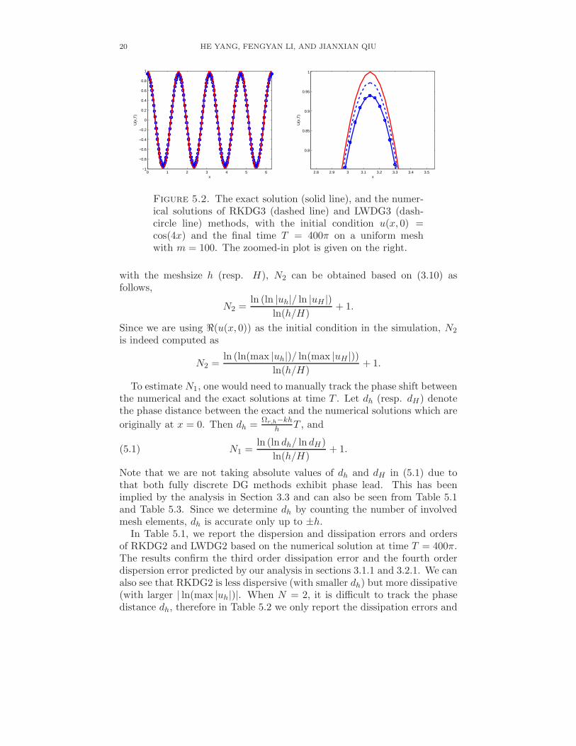
ν = 0.2 for LWDG2, ν = 0.2 for RKDG3, and ν = 0.1 for LWDG3. In Figure5.1, we plot the numerical solutions of RKDG2 and LWDG2 methods withm = 100 and T = 400π. One can see that the RKDG2 is more dissipative.The solutions by RKDG3 and LWDG3 methods are given in Figure 5.2 onthe same mesh at T = 400π. Apparently, these two third order methodsperform much better than the second order ones. In fact, one would needto zoom in the plot (see the one on the right in Figure 5.2) in order tosee the difference among the two numerical solutions and the exact solution.This zoomed-in plot also shows that the LWDG3 method is more dissipativethan the RKDG3 method. These qualitative observations are consistent toour theoretical analysis. What one cannot directly extract from these twofigures is the phase error in the numerical solutions.

0 1 2 3 4 5 6−1

−0.8

−0.6

−0.4

−0.2

0

0.2

0.4

0.6

0.8

1

x

U(x

,T)

Figure 5.1. The exact solution (solid line), and the numer-ical solutions of RKDG2 (dashed line) and LWDG2 (dash-circle line) methods, with the initial condition u(x, 0) =cos(4x) and the final time T = 400π on a uniform meshwith m = 100.

Next, we will examine the dissipation and dispersion errors quantitativelyand verify the analytical results in section 3. More specifically, we want toestimate the orders N1 and N2 in the dispersion error Ωr−K = O(KN1) andthe dissipation error Ωi = O(KN2). With the initial condition u(x, 0) = eikx

and the numerical solution uh (resp. uH) computed from a uniform mesh


0 1 2 3 4 5 6−1

−0.8

−0.6

−0.4

−0.2

0

0.2

0.4

0.6

0.8

1

x

U(x

,T)

2.8 2.9 3 3.1 3.2 3.3 3.4 3.5

0.8

0.85

0.9

0.95

1

x

U(x

,T)

Figure 5.2. The exact solution (solid line), and the numer-ical solutions of RKDG3 (dashed line) and LWDG3 (dash-circle line) methods, with the initial condition u(x, 0) =cos(4x) and the final time T = 400π on a uniform meshwith m = 100. The zoomed-in plot is given on the right.

with the meshsize h (resp. H), N2 can be obtained based on (3.10) asfollows,

N2 =ln (ln |uh|/ ln |uH |)

ln(h/H)+ 1.

Since we are using ℜ(u(x, 0)) as the initial condition in the simulation, N2

is indeed computed as

N2 =ln (ln(max |uh|)/ ln(max |uH |))

ln(h/H)+ 1.

To estimate N1, one would need to manually track the phase shift betweenthe numerical and the exact solutions at time T . Let dh (resp. dH) denotethe phase distance between the exact and the numerical solutions which are

originally at x = 0. Then dh =Ωr,h−kh

hT , and

(5.1) N1 =ln (ln dh/ ln dH)

ln(h/H)+ 1.

Note that we are not taking absolute values of dh and dH in (5.1) due tothat both fully discrete DG methods exhibit phase lead. This has beenimplied by the analysis in Section 3.3 and can also be seen from Table 5.1and Table 5.3. Since we determine dh by counting the number of involvedmesh elements, dh is accurate only up to ±h.

In Table 5.1, we report the dispersion and dissipation errors and ordersof RKDG2 and LWDG2 based on the numerical solution at time T = 400π.The results confirm the third order dissipation error and the fourth orderdispersion error predicted by our analysis in sections 3.1.1 and 3.2.1. We canalso see that RKDG2 is less dispersive (with smaller dh) but more dissipative(with larger | ln(max |uh|)|. When N = 2, it is difficult to track the phasedistance dh, therefore in Table 5.2 we only report the dissipation errors and


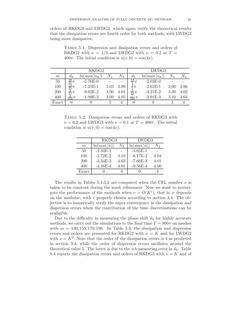
orders of RKDG3 and LWDG3, which again verify the theoretical resultsthat the dissipation errors are fourth order for both methods, with LWDG3being more dissipative.

Table 5.1. Dispersion and dissipation errors and orders ofRKDG2 with ν = 1/3 and LWDG2 with ν = 0.2 at T =400π. The initial condition is u(x, 0) = cos(4x).

RKDG2 LWDG2m dh ln(max |uh|) N1 N2 dh ln(max |uh|) N1 N2

50 4925π -5.76E-0 - - 12

5 π -2.03E-0 - -100 12

25π -7.25E-1 3.03 3.99 35π -2.61E-1 3.00 3.96

200 325π -9.02E-2 3.00 4.01 3

20π -3.21E-2 3.00 4.02400 3

100π -1.09E-2 3.00 4.05 7200π -3.91E-3 3.10 4.04

Exact 0 0 3 4 0 0 3 4

Table 5.2. Dissipation errors and orders of RKDG3 withν = 0.2 and LWDG3 with ν = 0.1 at T = 400π. The initialcondition is u(x, 0) = cos(4x).

RKDG3 LWDG3m ln(max |u|) N2 ln(max |u|) N2

50 -2.34E-1 - -5.05E-1 -100 -2.72E-2 4.10 -6.17E-2 4.04200 -3.34E-3 4.03 -7.66E-3 4.01400 -4.16E-4 4.01 -9.56E-4 4.00

Exact 0 4 0 4

The results in Tables 5.1-5.2 are computed when the CFL number ν istaken to be constant during the mesh refinement. Now we want to investi-gate the performance of the methods when ν = O(Kr), that is, ν dependson the meshsize, with r properly chosen according to section 3.4. The ob-jective is to numerically verify the super-convergence in the dissipation anddispersion errors when the contribution of the time discretizations can benegligible.

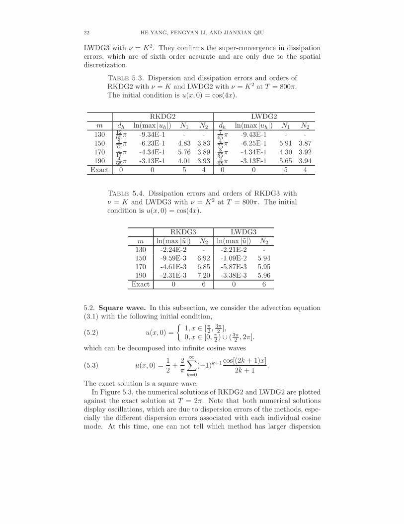
Due to the difficulty in measuring the phase shift dh for highly accuratemethods, we carry out the simulations to the final time T = 800π on mesheswith m = 130, 150, 170, 190. In Table 5.3, the dissipation and dispersionerrors and orders are presented for RKDG2 with ν = K and for LWDG2with ν = K2. Note that the order of the dissipation errors is 4 as predictedin section 3.4, while the order of dispersion errors oscillates around thetheoretical value 5. The latter is due to the ±h measuring error in dh. Table5.4 reports the dissipation errors and orders of RKDG3 with ν = K and of


LWDG3 with ν = K2. They confirms the super-convergence in dissipationerrors, which are of sixth order accurate and are only due to the spatialdiscretization.

Table 5.3. Dispersion and dissipation errors and orders ofRKDG2 with ν = K and LWDG2 with ν = K2 at T = 800π.The initial condition is u(x, 0) = cos(4x).

RKDG2 LWDG2m dh ln(max |uh|) N1 N2 dh ln(max |uh|) N1 N2

130 1265π -9.34E-1 - - 7

65π -9.43E-1 - -150 8

75π -6.23E-1 4.83 3.83 475π -6.25E-1 5.91 3.87

170 117π -4.34E-1 5.76 3.89 3

85π -4.34E-1 4.30 3.92190 4

95π -3.13E-1 4.01 3.93 295π -3.13E-1 5.65 3.94

Exact 0 0 5 4 0 0 5 4

Table 5.4. Dissipation errors and orders of RKDG3 withν = K and LWDG3 with ν = K2 at T = 800π. The initialcondition is u(x, 0) = cos(4x).

RKDG3 LWDG3m ln(max |u|) N2 ln(max |u|) N2

130 -2.24E-2 - -2.21E-2 -150 -9.59E-3 6.92 -1.09E-2 5.94170 -4.61E-3 6.85 -5.87E-3 5.95190 -2.31E-3 7.20 -3.38E-3 5.96

Exact 0 6 0 6

5.2. Square wave. In this subsection, we consider the advection equation(3.1) with the following initial condition,

(5.2) u(x, 0) =

1, x ∈ [π2 ,3π2 ],

0, x ∈ [0, π2 ) ∪ (3π2 , 2π].

which can be decomposed into infinite cosine waves

(5.3) u(x, 0) =1

2+

2

π

∞∑

k=0

(−1)k+1 cos[(2k + 1)x]

2k + 1.

The exact solution is a square wave.In Figure 5.3, the numerical solutions of RKDG2 and LWDG2 are plotted

against the exact solution at T = 2π. Note that both numerical solutionsdisplay oscillations, which are due to dispersion errors of the methods, espe-cially the different dispersion errors associated with each individual cosinemode. At this time, one can not tell which method has larger dispersion


error. On the other hand, the magnitude of the oscillation in RKDG2 so-lutions is relatively smaller, this indicates that RKDG2 is more dissipative,just as predicted by the theoretical result in section 3 for a single wave mode.

The analysis in section 3 implies that higher order methods have betterdissipation and dispersion behavior and therefore more accurate results, thiscan be demonstrated by Figure 5.4 which includes the solutions of RKDG3and LWDG3. Note that these solutions have much smaller oscillations thanthe solutions by second order schemes, and the shape is also very close to thesquare wave. In order to compare the dissipation behaviors of RKDG3 andLWDG3, we continue the simulation and plot the solutions after 2.5 × 104

time periods in Figure 5.5. One can easily see that the LWDG3 is moredissipative and this agrees with our theoretical result in section 3.3. For thesimulation in this subsection, we take the CFL number ν = 1

3 for RKDG2,ν = 0.2 for LWDG2, ν = 0.2 for RKDG3, and ν = 0.1 for LWDG3.

0 1 2 3 4 5 6

−0.2

0

0.2

0.4

0.6

0.8

1

1.2

x

U(x

,T)

0 1 2 3 4 5 6

−0.2

0

0.2

0.4

0.6

0.8

1

1.2

x

U(x

,T)

Figure 5.3. Solutions by RKDG2 (left) and LWDG2(right), with a square wave initial condition (5.2) and thefinal time T = 2π on a uniform mesh with m = 40. The solidline and dash-circle line represent the exact solution and thenumerical solution, respectively.

6. Concluding remarks

In this paper, the dispersion and dissipation errors are analyzed for discon-tinuous Galerkin methods. We focus on fully discrete discontinuous Galerkinmethods and their analytical discrete dispersion relation as a function of theCFL number ν in the limit of K = kh → 0. With the results, a quantitativecomparison is made between Runge-Kutta discontinuous Galerkin methods(RKDG) and Lax-Wendroff discontinuous Galerkin methods (LWDG). Inparticular, for RKDG2 and LWDG2, the dominating error comes from dis-persion, and RKDG2 has smaller dispersion error but larger dissipation errorthan LWDG2. However, RKDG3 has better dispersion and dissipation be-havior than LWDG3. An alternative dispersion analysis, by assuming thewave frequency is given, proves to be advantageous for the one-step LWDG


0 1 2 3 4 5 6

0

0.2

0.4

0.6

0.8

1

x

U(x

,T)

0 1 2 3 4 5 6

0

0.2

0.4

0.6

0.8

1

x

U(x

,T)

Figure 5.4. Solutions by RKDG3 (left) and LWDG3(right), with a square wave initial condition (5.2) and thefinal time T = 2π on a uniform mesh with m = 40. The solidline and dash-circle line represent the exact solution and thenumerical solution, respectively.

0 1 2 3 4 5 6

0

0.2

0.4

0.6

0.8

1

x

U(x

,T)

0 1 2 3 4 5 6

0

0.2

0.4

0.6

0.8

1

x

U(x

,T)

Figure 5.5. Solutions by RKDG3 (left) and LWDG3(right), with a square wave initial condition (5.2) and thefinal time T = 5 × 104π on a uniform mesh with m = 40.The solid line and dash-circle line represent the exact solu-tion and the numerical solution, respectively.

methods of arbitrary order of accuracy. This approach avoids solving aneigenvalue problem of a growing size when the accuracy order of the methodincreases.

By considering the dispersion and dissipation errors with sufficiently smallCFL numbers, we also find that the DG spatial discretizations contributesto super-convergence in dissipation and dispersion errors, while the Runge-Kutta or Lax-Wendroff time discretizations with matching accuracy willreduce or eliminate such super-convergence when the CFL number is takento be order one as in common practice. We believe this difference is due tothat DG spatial discretizations are of finite element type, while the temporaldiscretizations in both RKDG and LWDG methods are of finite difference


type. To avoid or to reduce the loss of the super-convergence property, onecan use ν = O(Kr) with some r > 0. That is, the CFL number dependson the meshsize and the characteristic wavenumber. Alternatively, whenν is chosen to be O(1), one can employ higher order Runge-Kutta timediscretizations for RKDG methods. In both cases, additional computationalcost is needed. For LWDG methods with ν = O(1), completely differentstrategies need to be explored in order to preserve the super-convergence indissipation and dispersion errors. This is currently under investigation.

The analysis in this paper is for the simple one dimensional scalar advec-tion equation. One can also conduct similar dispersion analysis for higherdimensional or systems of wave equations. Though the actual analysis oftendepends on the choice of the discrete spaces and mesh elements, in somecases, it can be essentially one dimensional and scalar. For example, thedispersion analysis of RKDG methods for higher dimensional scalar advec-tion equation can be reduced to the study of several one dimensional scalaradvection equations, when the Cartesian mesh is used together with discretespaces of tensor structure.

References

[1] N. N. Abboud and P. M. Pinsky, Finite-element dispersion analysis for the 3-dimensional 2nd-order scalar wave-equation, International Journal for NumericalMethods in Engineering, 35 (1992), pp. 1183-1218.

[2] M. Ainsworth, Dispersive and dissipative behavior of high order discontinuousGalerkin finite element methods, Journal of Computational Physics, 198 (2004),pp.106-130.

[3] M. Ainsworth, Discrete dispersion relation for hp-version finite element approxima-tion at high wave number, SIAM Journal on Numerical Analysis, 42 (2004), pp.553-575.

[4] M. Ainsworth, P. Monk and W. Muniz, Dispersive and dissipative properties of dis-continuous Galerkin finite element methods for the second-order wave equation, Jour-nal of Scientific Computing, 27 (2006), pp. 5-60.

[5] M. Ainsworth and H. A. Wajid, Dispersive and dissipative behavior of the spectralelement method, SIAM Journal on Numerical Analysis, 47 (2009), pp. 3910-3937.

[6] M. Ainsworth and H. A. Wajid, Explicit discrete dispersion relations for the acousticwave equation in d-dimensions using finite element, spectral element and optimallyblended schemes, Computer Methods in Mechanics, 1 (2010), pp. 3-17.

[7] G. Chavent and G. Salzano, A finite element method for the 1d water flooding problemwith gravity, Journal of Computational Physics, 45 (1982), pp.307-344.

[8] B. Cockburn and C. W. Shu, The Runge-Kutta local projection P1-discontinuous

Galerkin method for scalar conservation laws, Mathematical Modelling and NumericalAnalysis, 25 (1991), pp.337-361.

[9] B. Cockburn and C. W. Shu, TVB Runge-Kutta local projection discontinuousGalerkin finite element method for conservation laws II: general framework, Mathe-matics of Computation, 52 (1989), pp.411-435.

[10] J.S. Hesthaven and T. Warburton, Nodal high order methods on unstructured grids:I. time-domain solution of Maxwell’s equations, Journal of Computational Physics,181 (2002), pp. 186-221.


[11] F. Hu and H. Atkins, Eigensolution analysis of the discontinuous Galerkin methodwith non-uniform grids, part I: one space dimension, Journal of ComputationalPhysics, 182 (2002), pp. 516-545.

[12] F. Hu, M. Hussaini and P. Rasetarinera, An analysis of the discontinuous Galerkinmethod for wave propagation problems, Journal of Computational Physics, 151(1999), pp.921-946.

[13] F. Ihlenburg and I. Babuska, Dispersion analysis and error estimation of Galerkin fi-nite element methods for the Helmholtz equation, International Journal for NumericalMethods in Engineering, 38 (1995), pp.3745-3774.

[14] C. Johnson and J. Pitkaranta, An analysis of the discontinuous Galerkin method fora scalar hyperbolic equation, Mathematics of Computation, 46 (1986), pp.1-26.

[15] P. Lesaint and P. A. Raviart, On a finite element method for solving the neutrontransport equation, Mathematical Aspects of Finite Elements in Partial DifferentialEquations, Academic Press, New York, 1974, pp. 89-123.

[16] T. Peterson, A note on the convergence of the discontinuous Galerkin method fora scalar hyperbolic equation, SIAM Journal on Numerical Analysis, 28 (1991), pp.133-140.

[17] J. Qiu, A numerical comparison of the Lax-Wendroff discontinuous Galerkin methodbased on different numerical fluxes, Journal of Scientific Computing, 30 (2007), pp.345-367.

[18] J. Qiu, D. Michael and C.-W. Shu, The discontinuous Galerkin method with Lax-Wendroff type time discretizations, Computer Methods in Applied Mechanics andEngineering, 194 (2005), pp.4528-4543.

[19] W. H. Reed and T. R. Hill, Triangular mesh methods for the neutron transportequation, Technical Report LA-UR-73-479 (1973), Los Alamos Scientific Laboratory.

[20] G. R. Richter, An optimal-order error estimate for the discontinuous Galerkinmethod, Mathematics of Computation, 50 (1988), pp.75-88.

[21] D. Sarmany, M. A. Botchev and J.J.W. van der Vegt, Dispersion and dissipation er-ror in high-order Runge-Kutta discontinuous Galerkin discretizations of the Maxwellequations, Journal of Scientific Computing, 33 (2007), pp.47-74.

[22] S. Sherwin, Dispersive analysis of the continuous and discontinuous Galerkin formu-lations, lecture notes.

[23] D. Stanescu, D. A. Kopriva and M. Y. Hussaini, Dispersive analysis for discontinuousspectral element methods, Journal of Scientific Computing, 15 (2000), pp.149-171.

[24] Q. Zhang and C.-W. Shu, Error estimates to smooth solution of Runge-Kutta discon-tinuous Galerkin methods for scalar conservation laws, SIAM Journal on NumericalAnalysis, 42 (2004), pp. 641-666.

[25] Q. Zhang and C.-W. Shu, Error estimates to smooth solution of Runge-Kutta dis-continuous Galerkin methods for symmetrizable conservation laws, SIAM Journal onNumerical Analysis, 44 (2006), pp. 1702-1720.

[26] Q. Zhang and C.-W. Shu, Stability analysis and a priori error estimates to the thirdorder explicit Runge-Kutta discontinuous Galerkin method for scalar conservationlaws, SIAM Journal on Numerical Analysis, 48(2) (2010), pp. 772-795.

[27] X. Zhong and C.-W. Shu, Numerical resolution of discontinuous Galerkin methodsfor time dependent wave equations, Computer Methods in Applied Mechanics andEngineering, 200 (2011), pp. 2814-2827.


Department of Mathematical Sciences, Rensselaer Polytechnic Institute,

110 8th Street, Troy, New York, 12180, USA

E-mail address: [email protected]

Department of Mathematical Sciences, Rensselaer Polytechnic Institute,

110 8th Street, Troy, New York, 12180, USA


School of Mathematical Science, Xiamen University, Xiamen, Fujian, 361005,

P.R. China


dispersion and dissipation errors of two fully

Documents