discretization and learning of bayesian networks using
TRANSCRIPT


Discretization and Learning of Bayesian Networks using Stochastic Search, with
Application to Base Realignment and Closure (BRAC)
A dissertation submitted in partial fulfillment of the requirements for the degree of Doctor of Philosophy at George Mason University
By
Pamela J. Hoyt Master of Science
George Mason University, 1996 Bachelor of Arts
University of Vermont, 1984
Director: Kathryn B. Laskey, Associate Professor Department of Systems Engineering
Spring Semester 2008 George Mason University
Fairfax, VA

ii
Copyright 2008 Pamela J. Hoyt All Rights Reserved

iii
DEDICATION
To my husband, Bruce, and my three sons, Hubbard, Benjamin and Thomas.

iv
ACKNOWLEDGEMENTS
I would like to thank the many friends, relatives, and supporters who have made this possible. My loving husband, Bruce, for his tremendous patience and support. Drs. Loerch and Driscoll who provided invaluable advice and assistance. I also thank the other members of my committee for their assistance. Finally, thanks to Dr. Kathy Laskey who believed I could finish and provided constant encouragement. The sage advice I carried with me from a fellow Vermonter, Calvin Coolidge, 30th President is: "Press on: nothing in the world can take the place of perseverance. Talent will not; nothing is more common than unsuccessful men with talent. Genius will not; unrewarded genius is almost a proverb. Education will not; the world is full of educated derelicts. Persistence and determination alone are omnipotent."

v
TABLE OF CONTENTS
.....................................................................................................................................Page List of Tables ................................................................................................................. vii List of Figures ..................................................................................................................ix Abstract .............................................................................................................................x 1. Introduction...................................................................................................................1
1.1 Objectives overview......................................................................................13 1.2 Methodology and Hypotheses overview.......................................................17 1.3 Summary .......................................................................................................18 1.4 Chapter Organization ....................................................................................20
2. Background.................................................................................................................22 2.1 Overview of the problem ..............................................................................22 2.2 Probability and Bayesian Networks..............................................................25 2.3 Learning Bayesian Networks........................................................................34
2.3.1 Learning BN from data ..................................................................34 2.3.2 Learning BN structure....................................................................43
2.4 Learning BN with continuous variables .......................................................47 2.4.1 Unsupervised discretization methods ............................................49 2.4.2 Supervised discretization methods.................................................50 2.4.3 Global verses local discretization methods....................................57 2.4.4 Outcomes of experiments ..............................................................58
2.5 Missing data and hidden variables................................................................62 2.6 Discretization and learning ...........................................................................67
2.6.1 PopMCMC method........................................................................67 2.6.2 BNPC method ................................................................................71
2.7 BRAC background........................................................................................75 3. Methodology...............................................................................................................82
3.1 Hypothesis I ..................................................................................................83 3.2 Hypothesis II.................................................................................................90 3.3 Hypothesis III................................................................................................91 3.4 Hypothesis IV ...............................................................................................92
4. Experiment..................................................................................................................95 4.1 Software implementation ..............................................................................95 4.2 Hypotheses testing ........................................................................................98
4.2.1 Hypothesis I .................................................................................100 4.2.2 Hypothesis II................................................................................123 4.2.3 Hypothesis III...............................................................................124 4.2.4 Hypothesis IV ..............................................................................126

vi
4.3 BRAC evaluation ........................................................................................130 5. Conclusion ................................................................................................................159 Appendix A: BRAC dataset..........................................................................................165 References.....................................................................................................................167

vii
LIST OF TABLES
Table ...........................................................................................................................Page 1.1. Discretization and learning methods........................................................................18 2.1. Conditional probability distribution for P(Smoking|Bronchitis) .............................27 2.2. Probabilities for Asia network example [Lauritzen and Spiegelhalter]...................31 2.3. Probabilities for Asia example ................................................................................32 2.4. Asia problem data observations for each state.........................................................39 2.5. Number of observations for each state in smoking..................................................42 2.6. Learning BN categories attributed to Myers (1999) ................................................42 2.7. Contingency table for classifying learning methods [Murphy, 01] .........................63 2.8. BRAC round acreage and time to disposal by percentage [Harris et al, 04] ...........77 2.9. BRAC round installation closure and disposal times [Harris et al, 04] ...................77 2.10. Results of correlation of variables in the BRAC data [Harris et al, 04] ................80 3.1. Discretization and learning methods........................................................................84 3.2. Design factors ..........................................................................................................86 3.3. Datasets for design study .........................................................................................87 3.4. Performance measures .............................................................................................89 4.1. Datasets for design of study.....................................................................................99 4.2. Software settings for initial data runs without interleaving ...................................100 4.3. Discretization policies............................................................................................101 4.4. Results of cutpoints for Asia data set.....................................................................102 4.5. Results of interleaving learning verse single step..................................................102 4.6. ‘True’ network structure BD scores.......................................................................105 4.7a. BN structure learned using PopMCMCPopMCMC method ...............................105 4.7b. BN structure learned using BNPC method ..........................................................106 4.8. Scoring result averages from Netica ......................................................................109 4.9. Comparison using equal width bins with PopMCMC and BNPC.........................111 4.10a. PopMCMC results..............................................................................................112 4.10b. BNPC results......................................................................................................112 4.11. Probabilities of species based on measurements .................................................116 4.12. Confusion and scoring matrix for the node Type ................................................117 4.13. Node names and description for diabetes data.....................................................118 4.14. Confusion and scoring matrix for the node Type for Diabetes data (1) ..............120 4.15. Confusion and scoring matrix for the node Type for Diabetes data (2) ..............121 4.16. PopMCMC results for percentage of missing data for Asia network..................123 4.17. PopMCMC results for 10 cycles 1000 iterations for Asia dataset.......................127 4.18. Arc count between nodes for Asia dataset...........................................................128 4.19. Correct Asia dependencies...................................................................................129

viii
4.20. Installations for BRAC study...............................................................................132 4.21. BRAC variable and node definitions ...................................................................134 4.22. Settings for BRAC data run .................................................................................135 4.23. Arc counts between nodes for BRAC data runs ..................................................136 4.24. Evidence entered on known nodes.......................................................................139 4.25. Cutpoints learned and prediction probabilities for BRAC data ...........................141 4.26. Sensitivity of years to dispose to other variables.................................................142 4.27. Sensitivity of years to close to other variables.....................................................143 4.28. Cutpoints and prediction probabilities for BRAC data holdouts .........................144 4.29. Node relationships based on arc counts for BRAC data......................................146 4.30. BRAC holdout installations for prediction capability .........................................147 4.31. Holdout prediction probabilities by category for BRAC.....................................148 4.32. Confusion matrix results for BRAC network ......................................................149 4.33. MACOM association with installation type ........................................................151 4.34. Evidence entered on node ....................................................................................152 4.35. Predictions with evidence for 37 installations .....................................................153 4.36. Predictions with evidence for 25 installations .....................................................154 4.37. Netica results of 1000 simulation of data ............................................................155

ix
LIST OF FIGURES
Figure ..........................................................................................................................Page 1.1. Smoking example divided into intervals....................................................................3 1.2. Hierarchical decomposition of discretization methods..............................................5 1.3. Discretization process [Liu et al, 02] .......................................................................10 2.1. Decision graph for two binary variables..................................................................26 2.2. Asia network from Lauritzen and Spiegelhalter, (88) .............................................30 2.3. A Bayesian Network for inferring the probability of S ...........................................35 2.4. Fragment of Asia network .......................................................................................38 2.5. Hierarchical framework for discretization methods ................................................49 2.6. A Bayesian Network with Plague as hidden variable..............................................64 2.7. A simple multi-connected network..........................................................................73 2.8. Connected structure learned by BNPC ....................................................................74 3.1. Systematic approach to Hypothesis I.......................................................................85 4.1. Asia BN of known and learned structures from PopMCMC.................................103 4.2. Sensor BN True Structure and Structure Learned byBNPC..................................103 4.3. BNPC modified learned structure for Asia data ....................................................107 4.4. Iris species based on sepal length and width .........................................................114 4.5. Netica network of Fisher’s iris data .......................................................................115 4.6. Netica network of diabetes data.............................................................................119 4.7. ROC for diabetes data............................................................................................122 4.8. Comparison of methods with percentage of missing value ...................................125 4.9. Learned BN in Netica for DPSC Philadelphia with evidence ...............................140 4.10. ROC curve for BRAC data ..................................................................................157

ABSTRACT
DISCRETIZATION AND LEARNING OF BAYESIAN NETWORKS USING STOCHASTIC SEARCH, WITH APPLICATION TO BASE REALIGNMENT AND CLOSURE (BRAC) Pamela J. Hoyt, PhD. George Mason University, 2008 Dissertation Director: Dr. Kathryn B. Laskey
The need for automated Bayesian Network (BN) construction from data has
increased for a variety of reasons. Elicitation of networks from experts can be time
consuming and expensive. With large, complex problems, construction of an accurate
network, which ‘best’ describe the probability distribution of the training data can be
difficult. The learning process is further complicated by missing or incomplete data, and
mixed data. In light of these issues BN construction cannot rely on experts alone, rather
experts can be used to enhance the network after the automated process. The closer
technology comes to building models that reflect the real world the more their power as
an inference tool will increase.
This research is an empirical approach on determining how well a stochastic
search discretizes continuous variables and learns structure. This study also has the
added complexity of missing data. Our approach interleaves discretization with a

stochastic search process to find a population of solutions for learning BNs. We
compared our process to other methods that discretize as a preprocessing step.
Learning BN structure as well as the parameters increases in difficulty when the
variables are continuous or mixed (both continuous and discrete). Real world datasets are
not generally discrete and missing data is common. Continuous variables are often
discretized in order to use one of the established and well-known learning algorithms.
Therefore, to handle the continuous variable the two common approaches are to apply a
discretization method or use one of the families of parametric distributions. The novel
approach we developed is a dynamic process that interleaves partitioning of continuous
variables with learning using a stochastic search method called PopMCMC.
We applied our new methodology to data from the U.S. Army’s recent Base
Realignment and Closure (BRAC) study from 1988 to 1995, which consists primarily of
both continuous and discrete variables complicated by missing data. The desired
outcome was to develop a method to model the BRAC data as a BN. A BN offered a
natural way to represent the uncertainties associated with the data and would then permit
us to make queries relevant to the BRAC decision making issues.

1
1 Introduction
Bayesian networks (BNs), also called belief networks, causal probabilistic
networks and Bayesian Belief Networks (BBN), are powerful tools for representing and
analyzing models that involve uncertainty and complexity. They are employed in a wide
range of disciplines to include engineering, medicine, business, military and law. Some
general tasks BNs perform include classification problems, general inference, prediction
(e.g. temporal), and planning. In the military, Bayesian networks help to predict enemy
actions [Mahoney, 99; Laskey et. al, 00]. The medical community uses BNs extensively
to assist with diagnosis of diseases [Heckerman, 90].
The interest in automated construction of Bayesian networks from data has
greatly increased since about the early 1990s [Cooper & Herskovits, 92, Bouckaert, 94,
Heckerman et al, 95]. This can be attributed to the amount of time and expense in
resources required to solicit expert human assistance in BN construction. As the
network’s size and complexity increases, the practice of engaging experts in an
interactive BN construction process becomes impractical at best and impossible at worst.
These knowledge-elicitation bottlenecks argue in favor of pursuing some means of
automatically constructing BNs directly from data.
Most current automated learning methods are designed to accommodate discrete
variables or discretized continuous variables, where the discretization is based on

2
cumulative density functions (CDFs) for random variables. Several authors [Dougherty
et al 95], and Kohavi and Sahami, 96], noted that the learning algorithms developed for
machine learning by Michalski and Stepp (1983), Cost and Salzberg (1993), Kohavi
(1994), and Apte and Hong (1996), for example, possessed limited utility in that their
application was limited to nominal feature spaces. As such, any continuous features
discretized using simple approaches such as equal width binning of data to construct the
required nominal features. For example, consider data with a continuous random variable
called ‘Smoking,’ which measures the average number of cigarettes smoked per day for a
host of individuals. This feature could be aggregated into smaller number of categories
by creating four bins: non-smoker ( p1) , light ( p2 ) , moderate ( p3) or heavy ( p4 ) and
subsequently partitioning the collected data according to preset bin width specifications.
Current commercial automated methods such as Bayesian Belief Network
Constructor, Hugin Expert, and Netica [Norsys Software Corp, 1995-2004], which
incorporate inductive algorithms for learning, require all continuous variables to be
discretized in advance. This is typically accomplished using a one-time preprocessing
stage built into the software application. This preprocessing stage fixes each variable’s
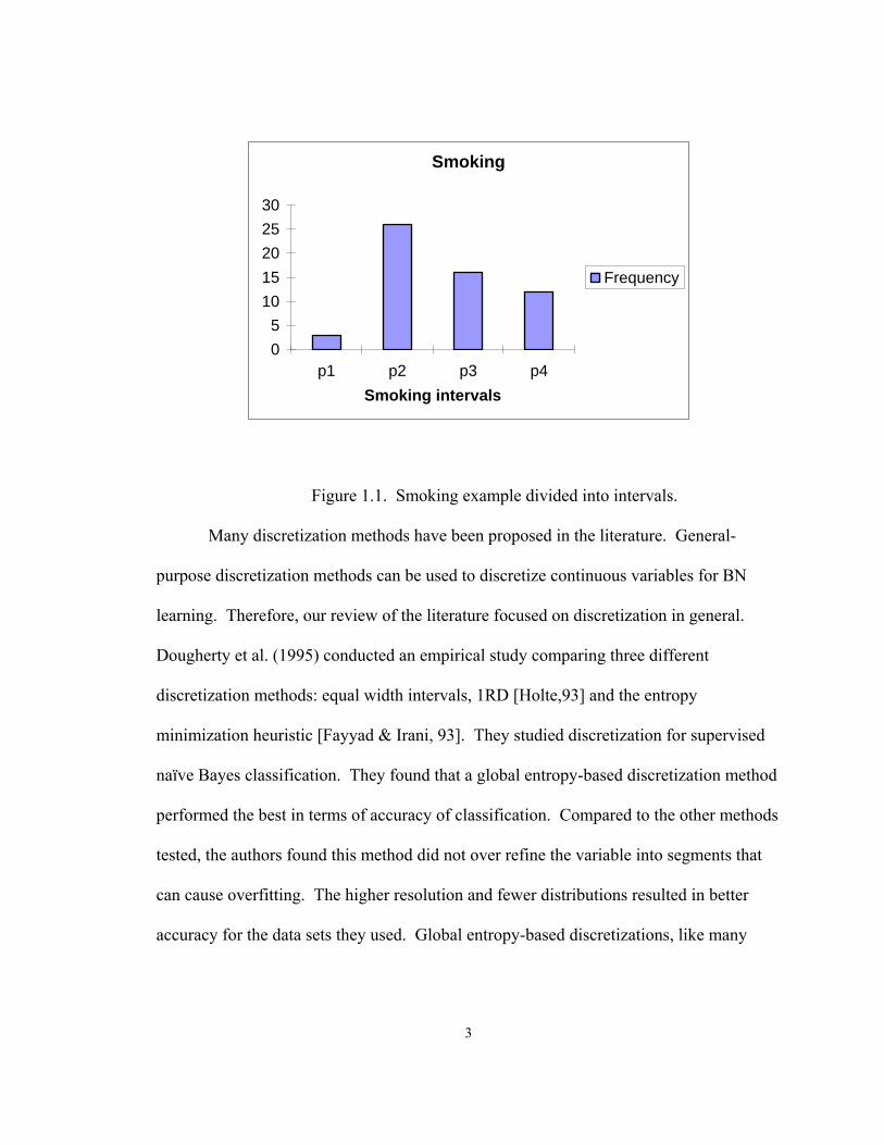
partitioning in a way that supports the subsequent structure learning process. Figure 1.1
illustrates the result of a hypothetical preprocessing step that would transform the
continuous random variable Smoking into a form that could be used by a structured
learning process that used the four nominal features defined earlier.
3
Smoking
05
1015202530
p1 p2 p3 p4Smoking intervals
Frequency
Figure 1.1. Smoking example divided into intervals.
Many discretization methods have been proposed in the literature. General-
purpose discretization methods can be used to discretize continuous variables for BN
learning. Therefore, our review of the literature focused on discretization in general.
Dougherty et al. (1995) conducted an empirical study comparing three different
discretization methods: equal width intervals, 1RD [Holte,93] and the entropy
minimization heuristic [Fayyad & Irani, 93]. They studied discretization for supervised
naïve Bayes classification. They found that a global entropy-based discretization method
performed the best in terms of accuracy of classification. Compared to the other methods
tested, the authors found this method did not over refine the variable into segments that
can cause overfitting. The higher resolution and fewer distributions resulted in better
accuracy for the data sets they used. Global entropy-based discretizations, like many

4
methods proposed in our literature search, are methods for finding the ‘right’ level of
resolution to accurately represent the original data.
To achieve the ‘right’ level of resolution, numerous methods and techniques have
been proposed for discretizing. It can be performed either as a preprocessing step to
learning or during learning. Discretization methods can be divided into five dichotomies
as supervised or unsupervised; and global or local; dynamic or static [Dougherty, et al.
95]; direct or incremental; and splitting top-down or merging bottom up. Supervised
discretization methods such as the Minimal Description Length (MDL) provide a natural
safeguard against overfitting because “ the winning model is the one with the lowest
combined complexity or description length”[Nannen, 03]. MDL methods are based on
the idea developed by Jorma Rissanen in 1978 using the principle in information theory
for inference. MDL uses a criterion that penalizes models based on a scoring process for
the number of parameters and for precision. The discretization that gives the shortest
description of the data is selected. The model that reduces the complexity by minimizing
the number of bits required to represent the data with respect to the network is chosen.
Conversely, unsupervised discretization methods such as equal interval are
sometimes called ‘class blind’ because they partition the data independent of the class
labels. Even if class information were available it is not used. For example, if the
measured feature is speed of the object, the equal width method divides the continuous
values into equal bin width as specified in advance. A problem with equal width or equal
frequency binning is deciding how to handle unequal number of observations or
repetitions of data points.
5
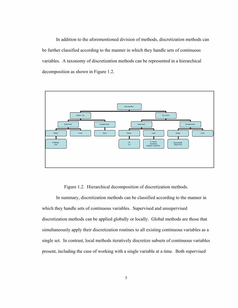
In addition to the aforementioned division of methods, discretization methods can
be further classified according to the manner in which they handle sets of continuous
variables. A taxonomy of discretization methods can be represented in a hierarchical
decomposition as shown in Figure 1.2.
Figure 1.2. Hierarchical decomposition of discretization methods.
In summary, discretization methods can be classified according to the manner in
which they handle sets of continuous variables. Supervised and unsupervised
discretization methods can be applied globally or locally. Global methods are those that
simultaneously apply their discretization routines to all existing continuous variables as a
single set. In contrast, local methods iteratively discretize subsets of continuous variables
present, including the case of working with a single variable at a time. Both supervised
Discretization
Bottom - Up Top -Down
Supervised UnsupervisedSupervised Unsupervised
Global Local
ChiMerge Chi2
None Global Local Global Local
D21R
K-meansClustering
Adaptive Quantizer
Equal Width Equal Freq
Discretization
Bottom - Up Top -Down
Supervised UnsupervisedSupervised Unsupervised
Global Local
ChiMerge Chi2
None Global Local Global Local
D21R
K-meansClustering
Adaptive Quantizer
Equal Width Equal Freq

6
and unsupervised discretization methods can also be partitioned bottom-up, top-down or
a combination of the two.
Both bottom-up and top-down discretization takes an ordered list of the data.
Bottom-up merges cut points and top-down adds cut points until the limit set by the user
is reached. Bottom-up discretization starts the process by imposing an initial set of cut
points over the range of values covered by the data. This is followed by merging
intervals during the discretization process. Returning to Figure 1.1, our smoking
example, if we had ordered data on the number of cigarettes smoked we could view every
data point as a potential partition element. A partition is a set of mutually exclusive and
collectively exhaustive partition elements. Using a bottom-up discretization process we
would merge partition elements until a stopping criteria was achieved. In Figure 1.1 we
have only four partition elements. Of course, a discretization process might have resulted
in more or fewer partition elements. Merging methods such as ChiMerge [Kerber, 92]
and Chi2 [Liu and Setiono, 97] are categorized as supervised because they use class
information to evaluate partitions. To evaluate the partitions they both use the Chi
squared statistical measure. ChiMerge allows the level of significance to be between 0.9
and 0.99 with a minimum of 5 partition elements and a maximum of 15. These settings
resulted in a good discretization of the data in previous the experiments [Kerber, 92; and
Liu et al, 02]. Chi2 is an automated version of ChiMerge that allows the level of
significance to vary. Merging of adjacent intervals continues until a criterion is met. In
both cases the chi square statistic is used to measure the relative class frequencies

7
between two intervals. If the measured frequencies are similar, intervals are combined.
Otherwise they remain separate.
Top down discretization, also referred to as splitting, adds cut points iteratively
until a stopping criterion is met. Top-down discretization begins with a single cut-point
that divides the data into two bins and continues to additional cut points are added during
the discretization process. The top-down or bottom-up methods can be either
unsupervised or supervised process. Unsupervised methods have a pre-established
number of bins and the data is divided equally among the bins. Two commonly used
unsupervised methods include equal width and equal frequency binning. Supervised
methods include entropy, binning, dependency or accuracy discretization methods as
shown in Figure 1.2.
Finally a dimension that cuts across the classification of Figure 1.2, but is not
shown, is whether discretization is static or dynamic. Static methods pass through the
data one time for each variable independent of the other variables. In static discretization
methods, the number of bins is usually determined and preset directly by the user as in
equal width binning and entropy-based partitioning methods such as D2 (Catlett, 91).
Alternatively, dynamic methods such as those employed by Freidman and Goldszmidt
(1996), examine all the interacting continuous variables sequentially in order to capture
the change to the variables parameter created by discretization. These methods
subsequently use this interaction information to determine an appropriate number of
intervals to accurately model the data. Such an iterative approach for discretization
repeatedly passes through the data until a particular stopping criterion is met.

8
For example, the Freidman and Goldszmidt discretization method begins with an
initial process that provides partitions based on lowest mean square error. It then
evaluates the direct descendents one at a time calculating the MDL score associated with
the discretization policy chosen. The process makes multiple passes until it reaches a
stopping criterion. Clarke and Barton [2000] proposed a similar method that discretizes
based on minimizing the MDL score. However, their discretization method discretizes
the data prior to initiating structured learning in the BN. An interesting feature of their
approach is that once the data is initially discretized, an iterative method is then
employed to dynamically repartition the continuous parent variables one at a time.
In examining which discretization policies improve accuracy, several authors
have found that the Naïve Bayes induction algorithm imbedded in the global entropy-
based discretization using the MDL metric performed slightly better than other
discretization methods but the results were not significant overall. To evaluate the
performance of the discretization methods based on prediction accuracy, the standard
deviations of the cross validations were compared using n-fold cross-validation method
[Dougherty, et al, 95; Friedman and Goldszmidt, 96]. More recent experiments have
shown that the general learning of Bayesian structures combined with either a global
entropy or clustering method outperforms the Naïve Bayes [Monti, 99; Lam and Low, 00;
Barton and Clarke, 00].
Liu et al. (2002) expanded upon the work of Dougherty et al (1995). They
demonstrated in their experiments with UCI repository data that selecting a discretization
method is a complex matter involving many factors. One key factor in selecting a

9
discretization method is whether or not class information is available. If class
information is available then there are numerous methods available for discretizing.
Shortcomings normally associated with unsupervised methods, such as effects caused by
outliers, or extreme observations can be overcome.
Liu et al. found that there are very few discretization methods that can be applied
when no class information is available. They found, in general that MDL performed well
overall in comparison to seven other methods (Equal width, 1R, D2, Mantara, Zeta,
ChiMerge and Chi2) with the strategy of imposing equal width binning performing the
worst.
Regardless of which discretization method is chosen, the general process can be
represented as the flow diagram illustrated in Figure 1.3. The flow chart below provides
a general outline of discretizing continuous variables.

10
Figure 1.3. Discretization process [Liu et. al, 02].
The discretization process, using the flow chart encompasses four steps: sorting,
evaluating the partitioning points, splitting or merging the partitions and stopping [Liu et.
al, 02]. The process starts by sorting the continuous data values. Candidate cut points
are selected iteratively or randomly for evaluation. Each candidate cut point is evaluated
using a scoring metric such as MDL, BD score or statistical measures such as Chi2.
Once evaluated, the cut points are adjusted either by merging or splitting in an attempt to
improve the score. This continues until a stopping criterion is met. The stopping
criterion can be based on a metric such as MDL or BD score, or can be set by the user.
Discretization of continuous variables has proven efficient and useful for machine
learning problems in that discretization can improve the overall speed of an induction
algorithm. Dougherty et al (1995) showed that not only does discretization reduce CPU
Sort Attribute
Get Cut Point/Adjacent Intervals
EvaluationMeasure
MeasureSatisfied
Split/MergeAttributes
StoppingCriterion
Continuous Attribute
No
No
Yes
Discretized Attribute
//Sorting continuous attribute
//Selecting a candidate cutpoint//or adjacent intervals
//Invokes appropriate measure
//Checks the outcome
//Discretize by splitting or//merging adjacent intervals
//Controls the overall discretization//based on some measure
Sorting
Evaluation
Splitting/Merging
Stopping
Yes

11
time but demonstrated that in some cases, depending on the learning algorithm, one has
the ability to improve the level of accuracy of predicting the class by discretizing the
continuous variables. They found, overall that entropy discretization method provided
the most significant improvement in accuracy.
As noted previously, discretization methods can be categorized as static, one pass
through the data set (equal width interval and 1R algorithm) or they can be dynamic.
Many of the dynamic methods reviewed use iterative heuristics, such as search and score
methods, and are generally capable of finding only local minimal solutions [Bradley and
Fayyad, 98, Kanungo, et. al., 00]. This problem is further exacerbated when there is
missing data. Stochastic search methods such as those presented by Myers (1999) can be
used to design effective global search algorithms that avoid becoming trapped at local
optima. Myers’ demonstrated how global information exchange could improve mixing
and speed up convergence thereby enabling the search to reaching a stationary
distribution rapidly. It follows that a promising approach to problems of mixed data
containing missing observations is a stochastic method that interleaves discretization with
learning of structure.
Learning the structure of a Bayesian network requires an extensive search over a
complex search space of parameters and structure. This challenge is compounded if there
are also missing data. Moreover, the question of how well the structure represents the
data may not be known for certain. These two challenges taken separately pose a high
level of difficulty. Taken alone, these problems are difficult; together it makes it even
more difficult for a belief network to learn a concise and accurate model. As Myers

12
points out, many times the one structure learned by a single model is considered the best
and is treated as “ground truth”. As an alternative approach, his research suggests that
multiple models may provide a better predictor than using a single model.
Our research had two objectives. The first objective was to conduct an empirical
methods study of discretizing continuous variables interleaved with learning of structure
when there is missing data in order to identify a combination of techniques that
effectively enhances structure identification and for classification. Our approach applied
various combinations of discretization methods and interleaved with a structure learning
method. We also examined the impact of missing data on discretization and learning.
The second objective was to apply the best resulting combination to a problem of
interest to the Army in order to demonstrate both its efficiency and its ability to reveal
novel insights concerning key decision factors. The problem of interest concerns
closures and realignment of Army installations. The bases are excess for a variety of
military and political reasons. The Deputy Assistant Secretary of the Army
(Infrastructure Analyses) and the Total Army Basing Study (TABS) Group would like to
speed up the closure process to reduce the costs incurred each year that the bases remain
under the control of the Army. Historical data have been collected since the inception of
the Base Realignment and Closure (BRAC) process in 1988. We applied our
discretization with interleaved learning to this BRAC data (1988-1996). Our goal was to
provide insights on the primary influence to closing and disposing of military
installations. A brief overview of both objectives is discussed as well as the four
hypotheses supporting our empirical study.

13
1.1 Objectives overview:
The first objective of this dissertation was to determine whether interleaving
discretization of continuous variables with learning of structure in Bayesian Belief
Networks improves structure identification accuracy and classification accuracy. A
further component of this objective was to evaluate the impact of learning with sparse
datasets. Based on the results of our literature search, we chose to employ a stochastic
search method to discretize the continuous variables and learn the network structure.
Unique to our approach, we extended the stochastic search method to propose a
population of solutions for missing data. This allowed us to evaluate the effects that
missing data imposes on discretization. Demonstrating our first stated objective
represented an improvement over current methods [Freidman and Goldszmidt, 95; Clarke
and Barton, 00; Pazzani, 95], principally through our use of automated methods [Hugin
®, Netica].
Current methods for discretizing continuous variables use a one-time
preprocessing stage to fix the variable partitioning to be used in the subsequent structure
learning process. While several researchers have shown such an approach yields
acceptable learning and classification results [Clarke and Barton, 00; Monti, 99], such a
myopic strategy suffers from two apparent shortcomings. First, potentially important
information is unused in that a one-time application of discretization cannot adjust
variable partitioning based on information gained during structural learning without
iterating repeatedly through the preprocessing routines. Secondly, for instances in which
the underlying structure is not known a priori, using preprocessing to discretize

14
continuous variables may not result in a learned network structure or structures that best
represents the data. A poor discretization may mask some of the underlying relationships
between variables or may introduce spurious relationships that are artifacts of
discretization.
Moreover, because information is shared globally across the network during the
learning process, interleaving provides a natural facility for partition re-adjustment, as
desired by performance thresholds. We conjectured that the end result would be a model
or models that allowed us to draw more accurate inference in response to probabilistic
queues.
As previously mentioned, we examined the consequences of introducing missing
data on the performance of the aforementioned interleaving approach. An ability to
handle missing data is essential because real world data typically involves missing or
severely corrupt data. Nevertheless, most current discretization methods work only with
complete data, typically, discarding missing data during the discretization process. When
global discretization is interleaved with learning, discarding missing data would result in
unacceptably small sample sizes. We show that an important advantage of our method is
that it can be applied in the presence of missing data without the detractors associated
with current methods. Understanding the impact of missing data on the performance of
our interleaving approach affords a further advantage to potentially improve the fidelity
of this method to the real world modeling requirements.
As a matter of course, we suspected that when the proportion of missing data is
small relative to the total sample size, adverse effects on either the discretization policy

15
or the structure learning should be minimal. However, as this proportion of missing data
increases we conjectured that there is a significant degradation in the performance of the
discretization policy. Herein, our methods were based on the assumption that absent data
is missing at random (MAR). MAR is defined as data on a variable X is missing at
random (MAR) if the probability of missing data on variable X is unrelated to the true
value [Allison, 01]. For our purposes, we assumed that any missing data is due to some
external influences. For example, participants in a drug rehabilitation program may be
less likely to return a survey that asks questions on his or her progress.
We had hypothesized that performance would degrade with increasing amounts of
missing data. The empirical study undertake in this work sought to enhance our
understanding of the tradeoff between performance of discretization policies and the
amount of missing data. Providing practioners with such insight affords them the ability
to could then assess the cost of collecting more data through additional surveys, call-
backs, and so on in comparison to potentially degraded performance. As a minimum, this
ability would advance the practice beyond a naïve application of methods.
The second objective of this dissertation was to apply our new methodology to the
problem of learning a BN that speeds up the Army’s Base Realignment and Closure
(BRAC) process by better understanding decision factors driving closure timeline. The
dataset was from the approved list of installations for closure or realignment from prior
BRAC rounds (88, 91, 93 and 1995). There were a total of 95 properties selected by the
BRAC Commission for closure or realignment. The data consists of 38 mixed features

16
that are nominal, discrete, and continuous. Additionally, the sample size was small with
regards to missing data.
There currently exists no BN model to assess the primary influences in closure
and disposition of installations. The Army Basing Study (TABS) office would like a
model that allows them to perform evaluations and predictions on installation closures
and disposition. Their goal for future BRACs is to close or realign 60% of the selected
installations within three years or less, and to dispose of 60% of the property within six
years or less. A recent study conducted on the Army BRAC process [Harris, et al., 04]
noted that the Army previously had used the time to dispose of a property as the primary
performance measure. This was changed to acreage of the property in later BRAC
rounds. However, the study concluded that there was no single factor that drives costs,
closure time and disposition time. Successfully applying our method to previous BRAC
rounds data provides a means of potentially identifying a combination of the key
variables that influencing the BRAC implementation process.
The development of a method to model the BRAC data as a BN offers a natural
way to represent the uncertainties associated with the BRAC data when dealing with
planning and prediction of base closing and disposition times. The subtle influences and
probabilistic interactions among the variables are more readily apparent in a BN. We
conjectured a BN learned from the data would provide insights to queries such as likely
amount of time to dispose a base if there is a large amount of unexploded ordnance
(UXO), the probability of closing 60% of the bases in 3 years, as well as Environmental

17
Protection Agency issues. The BN would permit us to make queries relevant to the
BRAC decision making issues.
1.2 Overview of Methodology and Hypotheses
With these objectives in mind the following hypotheses were investigated in this
dissertation:
Hypothesis 1:
When continuous variables are involved, interleaving discretization with learning
of structure will reduce the information loss due to discretization thus improving
classification performance.
Hypothesis 2:
Continuous variables with observations missing at random (MAR) can be
discretized successfully by combining a Monte Carlo method for filling in the missing
data with a stochastic search over discretization policies. As above, success is defined as
accuracy in response to queries.
Hypothesis 3:
The performance of a discretization algorithm shows a measurable degradation as
the amount of missing data increases. Through empirical study we can determine the
relationship between performance and the amount of missing data.
Hypothesis 4:
When structure is unknown, and/or there is a relatively large amount of missing
data, Arc counts over multiple structures and discretization policies will result in more
accurate inferences than using a single ‘best’ model.

18
To evaluate the first hypothesis we used two discretization methods (MCMC with
BD score and Hill Climbing with BD score) and two structure learning methods
(PopMCMC and BN Power Constructor) for the experiments (see Table 1.1).
Table 1.1. Discretization and learning methods.
Discretization Method Learning Structure Method 1. MCMC with BD score 1. PopMCMC 2. Hill Climbing (HC) with BD score 2. BN Power Constructor
Pairwise combinations of these discretization methods interleaved with the
learning algorithms were tested to find which one performed best. We compared the
algorithms with respect to accuracy of inference for probabilistic queries, speed of
inference, and speed of discretization.
Our test of the second hypothesis employed a Monte Carlo method to generate a
population of solutions for the missing data. We took a similar approach for hypothesis 3
but varied the percentage of missing observations to evaluate the effects on performance
of the discretization algorithm.
For the last hypothesis we examined how well conducting an arc count over
multiple structures when there is uncertainty associated with the data and one model does
not dominate the other models.
1.3 Summary
The need for automated BN construction from data has increased for a variety of reasons.
Elicitation of networks from experts can be time consuming and expensive. With large,

19
complex problems, construction of an accurate network which ‘best’ describe the
probability distribution of the training data can be difficult. The learning process is
further complicated by missing or incomplete data, and mixed or continuous and discrete
data. In light of these issues BN construction can be a time consuming task, especially
when there are a large number of variables. The closer technology comes to building
models that reflect the real world the more their power as an inference tool will increase.
The research examined the contribution of a stochastic process for interleaving
discretization and learning structure with missing data. Several methods for learning
structure with hidden variables and missing data exist [Friedman, 97]. There are also
numerous methods for discretization [Catlett, 91; Fayyad and Irani, 93; Pfahringer, 95;
Liu and Setiono, 95; Ho and Schott, 97]. Several authors have done comparative analysis
on discretization methods [Dougherty, et al, 95; Kohavi and Sahami, 96; Liu, et al, 02].
Authors such as Friedman and Goldszmidt have dealt with a combination of the issues:
learning BNs with missing data or learning BNs with continuous variables. However, to
our knowledge and after extensive research the problem of learning BN from data when
there is missing data and continuous variable has not been addressed together. The four
hypotheses relate to methods designed to overcome these problems.
To demonstrate potential use of our process, we applied our methodology to the
Army’s Base Realignment And Closure (BRAC) data. The data was comprised of mixed
random variables and provided an excellent dataset to further test our hypotheses. We
discuss BRAC in greater detail in the next chapter.

20
1.4 Chapter Organization
This study is organized as follows. Chapter 2 discusses the relevant literature to
our research. The chapter consists of seven sections. The first section provides a general
overview of the research. The second is an overview of Bayesian networks. The third
section focuses on learning Bayesian Networks from data, learning of structure and
scoring metrics for model selection. We then discuss in the fourth section learning BN
with continuous variables and methods for discretizing continuous variables for learning.
The fifth section discusses missing data and current methods to handle missing data in
learning and discretization. The sixth section is an overview of the discretization and
learning structure methods we used in the study. The last section provides background
and an overview of the BRAC process.
Chapter 3 is a detailed discussion of our methodology used for this research to
support our hypotheses. We discuss the two discretization methods we used (MCMC
with BD score and Hill Climbing with BD score). We also describe the two structure
learning methods we used (PopMCMC and BN Power Constructor) and their interleaving
as part of the discretization process. We discuss separately the process for handling
missing data, detailing how the process for missing data is integrated with interleaving
discretization with learning of structure.
Chapter 4 discusses the experimental design as well as our results. We discuss
both the test data and the BRAC data. This chapter follows the order set forth in chapter
3, first with the test data and then with the BRAC data. The results from the test and
BRAC data are compared based on the metrics established in chapter 3.

21
Chapter 5 concludes the study with a summary of the key insights learned as well
as future work.

22
2 Background
This chapter provides the necessary background and relevant concepts to
understand the methodology employed. The most relevant literature is also surveyed to
understand how our method varies from the other methods for learning Bayesian
networks with continuous variables. In order to understand our approach we begin with a
brief overview of the problem. The next section, 2.2, we provide a general overview of
Bayesian networks. This leads into the issue of learning BN from data, learning of
structure and scoring metrics for model selection, which will be discussed in section 2.3.
In section 2.4, we then discuss BNs with continuous variables and methods for
discretizing continuous variables for learning. A complication to learning structure is
missing data. Section 2.5 will discuss this issue and current methods to handle missing
data in learning and discretization. Section 2.6 is an overview of structure learning
methods, specifically PopMCMC and Belief Network Power Constructor (BNPC). The
last section is a discussion of BRAC.
2.1 Overview of the problem
Building BNs can be tedious and time consuming process especially when
working with large, complex real-world domains. Over the years, automated methods
for learning Bayesian networks from data have emerged. Generally, these algorithms
used for learning can be grouped into two categories. One category of algorithms uses

23
heuristic search method to construct a model and evaluates it using a scoring method.
This process continues until the score of the new model is not significantly better than the
old one. Different scoring criteria have been applied in these algorithms, such as
Bayesian scoring method [Cooper and Herskovits, 92], entropy based method
[Herskovits, 91], and minimum description length method [Suzuki, 96]. The other
category of algorithms constructs Bayesian networks by analyzing dependency
relationships among nodes. The dependency relationships are measured by using some
kind of conditional independence (CI) test [Cheng, Bell and Liu, 98]. However, the major
algorithms in literature apply only to discrete variables.
Learning BN structure as well as the parameters increases in difficulty when the
variables are continuous or mixed (both continuous and discrete). Many data sets are not
discrete. They are comprised of both continuous and discrete variables. The variables
are often discretized in order to use one of the established and well-known learning
algorithms. Therefore, to handle the continuous variables the two common approaches
are to apply a discretization method or use one of the families of parametric distributions
[Cheeseman, et al., 88; Heckerman and Geiger, 95; John and Langley, 95]. A common
parametric approach is to assume a Gaussian distribution for the continuous attributes to
model the data [Cobb, et al., 07].
The less costly of the two approaches is to discretize. Discretization reduces the
number of possible values for the continuous variable and is not bound to a specific
distribution. Additionally, computing the conditional probability for a continuous
random variable is difficult. Douhgery, Koharia and Sahami (1995) showed empirically

24
the benefits to discretizing. In most cases, the continuous variables are discretized as a
preprocessing step. The number of partitions are increased, for top down methods and
decreased for bottom up methods. The desire is generally to adjust the number of
partitions until no further improvement can be made to a particular evaluation score or
until the partitions exceed some fixed threshold number as set by the user. Both of these
approaches are static in the sense that partitioning is completed prior to any structure
learning begins. There is not a process available to dynamically partition the data while
learning.
Most current papers on learning Bayesian Networks with continuous variables, if
discretization is used, perform it as a preprocessing step [Friedman and Goldszmidt, 96;
Monti, 99; Clarke and Barton, 00] in the manner described. Only one approach addresses
dynamic discretization techniques for Bayesian Networks. These are only two examples,
Clarke and Barton (2000) and Friedman and Goldszmidt (1996), appear to be the only
published dynamic discretization methods for learning BNs and we were unable to find
any for multivariate discretization with missing data. Moreover, both of these efforts
assume full or partial node ordering. The dynamic process we introduce in chapter 3
addresses the issue of learning structure when node ordering is not known.
Clarke and Barton (2000) proposed a process to dynamically repartition
continuous variables. Unlike the process we introduce herein, their process focused on
the continuous variables independently, ignoring the interaction with other variables.
Their process first partitions the continuous variables as a preprocessing step and then
attempts to find additional partitions in a recursive manner. They concluded that their

25
dynamic repartitioning of the continuous variables did not significantly improve the score
over the preprocessing partitioning method.
Bayesian Network (BN) models provide an effective method for associating a
large number of variables and communicating their relationships through a graphical
representation. Their compact representation of probabilistic information permits one to
investigate relationships based on known conditional independencies existing among
variables and to make predictions through queries of the network. Another advantageous
aspect is that BNs are easy to update as new information or evidence becomes available
[Lauritzen and Spiegelhalter, 88].
In the section that follows, we use Lauritzen and Speigelhalter’s Asia network
example for Dyspnea (shortness of breath) throughout this chapter due to its simplicity to
illustrate many of the aforementioned characteristics. Even though all the nodes are
discrete we will convert some to continuous variables to show the various methods.
2.2 Probability and Bayesian Networks
Probability theory is employed in many disciplines to express knowledge about
uncertain events or processes. In the medical field, a physician may make observations
about a patient. The physician will use the information from the patient’s symptoms and
medical history to diagnose the problem. The expert, (i.e. the physician) uses
observations about the state of the world to determine actions (i.e. treat or don’t treat). In
attempting to represent the world there is always uncertainty due to incomplete
information, lack of knowledge, and so on. How this uncertainty is represented can
impact our actions through incorrect conclusions or result in not achieving goals.

26
We can represent uncertain hypotheses and their relationships as a graph linking
causes to effects. For example, Figure 2.1 represents knowledge about the relationship
between Smoking and Bronchitis. The simple two-node graph in figure 2.1 is from a
larger model [Lauritzen and Spiegelhalter, 88].
Figure 2.1 Decision graph for two binary variables.
If we had knowledge that a patient was a smoker this would increase our belief
that the patient might have Bronchitis. We could also infer in the opposite direction that
if a patient has bronchitis he probably is a smoker. The arrow from Smoking to
Bronchitis represents the causal impact or dependency between the two nodes. It allows
us a means to reason about uncertainties. These uncertainties can be represented in a
mathematical model. Specifically, the graphical structure provides a means to represent
quantitative assumptions through a concise representation of the joint probabilities that
allows us to draw inference from observations [Pearl, 00].
The nodes in the graphical model represent random variables. For our simple two
node example we have limited our variables to two possible values. However, we could
have had any number of values to include continuous. Each variable in our example is
comprised of two states and for each state there is an associated probability. Only one
Smoking (S) Bronchitis (B)

27
state or event can occur at a time. Thus, the values are mutually exclusive and
collectively exhaustive.
We use the following notational convention in what follows. Upper case letters
denote random variables, e.g., S for Smoking and B for Bronchitis. States or values of
those variables are represented by strings beginning with lowercase letters, and are
indexed by subscripts as necessary, e.g., b or bi represent possible values of the random
variable B. For the example shown, S is to denote the variable Smoking with the values
of yes or no indicated as a1 and a2 respectively. Similarly, we use B for the variable
Bronchitis with b1 and b2 for the respective values, present or absent.
Each node has conditional probabilities that are conditioned on its parent in the
graph. In order to specify the dependency expressed in Figure 2.1, we need to specify
three quantities: the probability of being a smoker or not which is the prior probability;
the conditional probability of having B= present given S=yes; and the probability of B=
present given S=no. The conditional probabilities associated with our two node example
quantifies the dependencies in our BN. We can represent the conditional probabilities in
a concise table format.
Table 2.1 Conditional probability distribution for P(Smoking|Bronchitis).
Bronchitis (b1) Bronchitis=Present (b2 ) Bronchitis=Absent(a1) Smoker (0.5) 0.60 0.40 (a2 )Non-smoker (0.5) 0.30 0.70

28
Table 2.1 represents the conditional probability that Bronchitis is present or
absent under each hypothesis about whether the person is a smoker. The conditional
probability, P(B|Pa(B))=P(B|S) associated with the node formalized the relationship
between the parent node, S=Pa(B) and the child node, B for the variable Bronchitis.
From this relationship we can then obtain the joint probability distribution over both
random variables as:
P(B) = P(S)P(S | B) (2.1)
For a more general BN with n random variables, the joint distribution is:
1( , , ) ( | ( ))n i iP X X P X Pa X= Π… (2.2)
In equation 2.2, Pa(Xi) means the set of parents for Xi in the BN. The joint
probability P(x1,…,xn) is the probability that the random variables Xi have values xi for
all i=1,…, n. These probabilities must sum to one, where the summation is over all
combinations of possible values for all n random variables. To specify a joint probability
distribution for our simple two node network, we would need only to specify 2n values
for a total of four entries. As the network becomes larger the calculations required to
apply Bayes rule become computationally intensive. Inference in Bayesian networks is
known to be NP-hard [Cooper, 90].
The probabilities associated with a random variable can be viewed as a means of
measuring the strength of the relationship between a variable and its parents. Bayes rule
allows us to evaluate the overall strength of our belief in a hypothesis based on prior
information and evidence. Through probabilistic inference we can answer queries about

29
the probability of a random variable given values of other random variables. These
queries are answered by applying Bayes Rule:
1 1 11 1
1 1 1 1 2 2
( | ) ( )( | )( | ) ( ) ( | ) ( )
P B b S a P S aP S a B bP B b S a P S a P B b S a P S a
= = == = =
= = = + = = =,
where the b1, b2, and a1 are abbreviations for yes, no, and present, respectively.
In our two node example, using the relationship between Smoking and Bronchitis
we were able to show causes and effects first through the graph and then numerically
with the probability tables. A Bayesian network allows us to express probabilistic
dependencies among many random variables. As stated previously, probabilistic
inference becomes more complex as the number of variables in the network increases.
For example, let us consider a larger network from a notional medical domain [Lauritzen
and Spiegelhalter, 88]. Each of the variables in the network has a finite set of mutually
exclusive states, two per variable for this example. This BN has a total of eight variables
with arrows or directed edges between the variables to indicate the relationship between
the nodes.
In a Bayesian network, directed cycles are not permitted. The variables and the
directed edges form what is known as a directed acyclic graph (DAG) as shown in Figure
2.2. Probability information associated with each of the nodes is expressed as a
conditional probability table (CPT). Figure 2.3 shows the CPTs for the Bayesian network
of Figure 2.2. The graph and the CPT together represent a joint distribution over the
random variables in the Bayesian network.

30
Figure 2.2. Asia network from Lauritzen and Spiegelhalter, (88).
Figure 2.2 shows an example of a Bayesian network that represents a simplified
problem in medical diagnosis. The graph structure indicates that tuberculosis and lung
cancer can cause an abnormality in the chest. Either can cause a positive x-ray or
dyspnea (shortness of breath). Bronchitis also causes dyspnea. A visit to Asia may
expose a person to tuberculosis. Smoking can cause both lung cancer and bronchitis.
The edges between nodes represent a direct dependency. For example,
tuberculosis is likely to be caused by a visit to Asia. However, there is not an edge
between the nodes Smoking (S) and Visit to Asia (A). This represents the assumption
that there is no direct dependence relationship between the two random variables.
Because they have no common ancestor, there is no indirect dependence either.
Therefore, we can state that the random variables, S (Smoking) and A (Visit to Asia) are
independent. Additionally, the graph implies that the random variables A (Visit to Asia)
and AC (Abnormality In Chest) are conditionally independent given the random variable
T (Tuberculosis). In general, a node is conditionally independent of all its non-
Tuberculosis
or Cancer: TC
Lung Cancer: L Bronchitis: B
Smoking: S
Dyspnea : DX - Ray Result: X
Tuberculosis: T
Visit To Asia: A
Asia
Abnormality
In Chest: AC
Lung Cancer: L Bronchitis: B
Smoking: S
Dyspnea : DX - Ray Result: X
Tuberculosis: T
Visit To Asia: A
Asia
Tuberculosis
or Cancer: TC
Lung Cancer: L Bronchitis: B
Smoking: S
Dyspnea : DX - Ray Result: X
Tuberculosis: T
Visit To Asia: A
Asia
Abnormality
In Chest: AC
Lung Cancer: L Bronchitis: B
Smoking: S
Dyspnea : DX - Ray Result: X
Tuberculosis: T
Visit To Asia: A
Asia
31
descendents given its parents. This is often referred to as the causal Markov condition
[Pearl, 00].
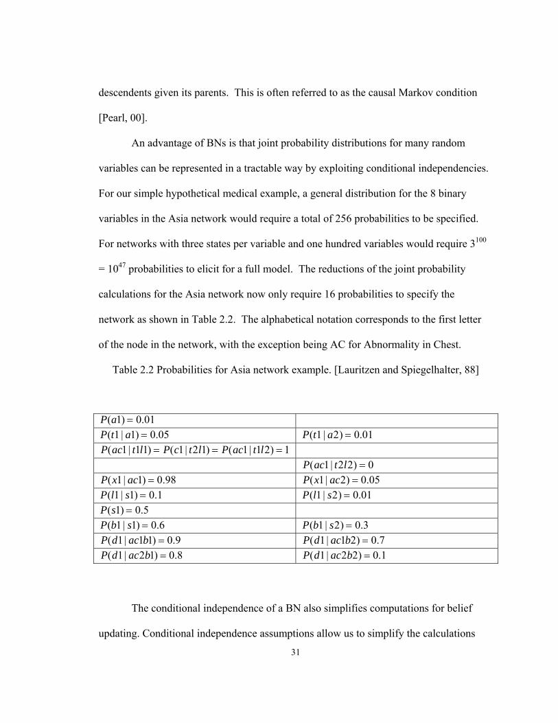
An advantage of BNs is that joint probability distributions for many random
variables can be represented in a tractable way by exploiting conditional independencies.
For our simple hypothetical medical example, a general distribution for the 8 binary
variables in the Asia network would require a total of 256 probabilities to be specified.
For networks with three states per variable and one hundred variables would require 3100
= 1047 probabilities to elicit for a full model. The reductions of the joint probability
calculations for the Asia network now only require 16 probabilities to specify the
network as shown in Table 2.2. The alphabetical notation corresponds to the first letter
of the node in the network, with the exception being AC for Abnormality in Chest.
Table 2.2 Probabilities for Asia network example. [Lauritzen and Spiegelhalter, 88]
P(a1) = 0.01 P(t1 | a1) = 0.05 P(t1 | a2) = 0.01
P(ac1| t1l1) = P(c1| t2l1) = P(ac1| t1l2) = 1 P(ac1| t2l2) = 0
P(x1| ac1) = 0.98 P(x1| ac2) = 0.05 P(l1 | s1) = 0.1 P(l1 | s2) = 0.01 P(s1) = 0.5 P(b1 | s1) = 0.6 P(b1 | s2) = 0.3
P(d1| ac1b1) = 0.9 P(d1| ac1b2) = 0.7
P(d1| ac2b1) = 0.8 P(d1| ac2b2) = 0.1
The conditional independence of a BN also simplifies computations for belief
updating. Conditional independence assumptions allow us to simplify the calculations

32
required for inference in a Bayesian Network [Jensen, 96; Neapolitan, 04]. In general,
BNs are a restricted class of models that can do inference and encode parsimonious but
accurate domain models.
The Bayesian network represented by the graph of Figure 2.2 and the CPTs of
Table 2.2 implicitly represents a joint probability distribution over the configuration of
the eight random variables from our Asia example. From this joint distribution we can
compute the marginal probability distribution of any individual variable. These marginal
probabilities are shown in the third column of Table 2.3.
Table 2.3. Probabilities for Asia example.
Asia network Variable State Prior probabilities
(no evidence) Evidence on Asia
and Dyspnea (A) Visit to Asia Yes 0.1 1.0
(S) Smoking Yes 0.5 0.62 (T) Tuberculosis Present 0.014 0.0876 (L) Lung cancer Present 0.055 0.0995 (B) Bronchitis Present 0.45 0.81
(TC) Tuberculosis or Lung cancer
Present 0.0648 0.81
(X) X-ray Abnormal 0.011 0.22 (D) Dyspnea Present 0.436 1.0
Table 2.3 shows the probabilities from the Asia network prior to receiving
information, ‘no evidence’ and the effects on each node once evidence is received. Only
one state is represented for each of the binary variables in the table. The fourth column
shows updated probabilities for all nodes after receiving evidence of a visit to Asia and

33
that the patient has dyspnea. When evidence is entered in the network, the probabilities
can be updated using Bayes rule. Once we have information on the variables, standard
belief propagation algorithms implement Bayes rule using computational methods that
exploit the structure of the network [Neapolitan, 04].
We have shown how the local probability distribution captures the probabilistic
relationship between nodes. Numerous algorithms exist for doing probabilistic inference
with BNs [Lauritzen and Spiegelhalter, 88; Pearl, 88; Jensen, 96; Heckerman, 95]. When
applied to problems such as the Asia network they allow the network calculations to be
computationally tractable. Standard algorithms apply only to discrete variables.
However, if the variables were continuous instead of discrete, there is no general-purpose
exact inference method. There are ways of calculating Bayes rule using special
algorithms but they require special assumptions about distributions. Approximation
techniques may be necessary.
In general, the necessary integrals do not have closed form solutions, thus
requiring an approximation. A common method for handling this problem is to assume a
Gaussian distribution for all continuous variables. Assuming a general parametric
representation, as previously noted can be infeasible [Dougherty, et al, 95; Friedman and
Goldszmidt, 96] and may result in a model that does not represent the data.
Discretization is an important approximation method for the general problem of inference
in BNs with continuous variables.

34
2.3 Learning Bayesian networks
The process of eliciting networks from experts can be tedious and time consuming
especially when working with large, complex real-world domains. Heckerman noted this
problem in his work in the late 1980s while developing an expert system called
Pathfinder. He found expert pathologists could map relationships when examining
features with which they were most familiar but could not map relationships outside of
their domains [Heckerman, 90]. There may also be situation in which an expert is not
available or whose expertise is limited to an area. To avoid depending on experts, a
method was needed to learn networks for the data.
2.3.1 Learning BN from data
The process of learning BN from data can be separated into two parts: learning
the parameters or probabilities, and learning the structure or graph [Heckerman 95,
Murphy 01]. In considering the first part, if we knew the structure then only the
parameters would need to be learned. This problem can be further simplified if we want
to learn the probabilities from data for only one variable. Consider the following figure
with several observations. The figure 2.3 shows a BN for the problem of inferring PS, the
probability of smoking, from a sample of n observations, S1, S2, … Sn.

35
Figure 2.3. A Bayesian network for inferring the probability of S.
In our BN, the random variable PS represents the probability that a patient is a
smoker. The value of this variable is between 0 and 1, and represents a probability that is
continuous. We want to learn the probability distribution for PS based on observations.
The set of random variables S1 to Sn are the observations of whether a patient smokes and
whose values are the outcomes (s1 for yes, and s2 for no). If we knew the true probability
of smoking, the problem would be simple, and we would write, P(Sn = s1 | PS ) = PS . To
calculate PS when it is unknown we use Bayesian inference. A simple method to
determine the probabilities PS would be to count the number of patients within our
sample that smoke. Using this information and the prior probability placed on PS, we
could then find the posterior distribution. This would represent our new probability for
the random variable PS.
In general, if we know the structure and have complete data we can use Bayes
rule to find the posterior distributions for all the CPTs. A typical approach to infer PS
from data is to assume that all of the observations are mutually independent conditional
Sn S1 S2
Ps
…
36
on the probability PS. Under this assumption, our sequence of random variables S1, …,
Sn, is a binomial sample of size n with parameter PS. Often a uniform prior is used to
represent a lack of knowledge about PS. As our sampling of patients increases, the
contribution of any prior distribution we might have assigned reduces relative to the
contribution of the observations. If the data has a lot of information then inferences are
insensitive to the prior distribution, and any convenient prior distribution will give similar
results. In this situation, a uniform prior distribution is often used for convenience.
Previously we had restricted ourselves to discrete uniform prior. The assumption
of a discrete uniform prior probability means that the probability distribution function,
f(p) is constant for all p. As an example of a BN with a uniform prior, our Asia example
could have 10 smokers and 10 nonsmokers. For this example we will assume a uniform
prior probability to express our lack of knowledge. After examining each of the 20
patients’ records we determine 10 are smokers. Since our binomial sample is discrete
and our prior is uniformly distributed over the interval [0, 1] we need a reasonable
approximation of our prior belief to find the posterior. In general terms, if k successes in
n trials and parameter π, the probability of success, then the conditional probability is,
(π | k) ∝π k (1− π )n−k (2.3)
We say that π has a beta distribution with parameters α and β, denoted as
Beta(α,β), if its density is of the form,
P(π ) ∝πα−1(1− π )β−1 (2.4)
Additionally, if π has a beta prior then it also has a beta posterior. The beta
distribution is from the conjugate family of continuous distributions, which allows us to
37
easily update our posterior distribution when our observations are discrete. Greater
details on the proof for the beta and binomial distribution are available in Lee (97).
Continuing with our example of the 20 patients, if from the records we determine
10 are smokers we could further state that our posterior distribution is beta with
parameters α=11 and β=11. In general, we count the number of patients that smoke,
denoted as s. The sample size is denoted as n. We can express the beta posterior in more
general terms with the two parameters as: s+1 and n-s+1.
As previously stated, since we did not have knowledge on the prior probability in
the previous example, we represented it as a uniform prior. This is also known as a
vague prior since it provides us very little information. For the beta distribution we
would then set α and β equal to one. In general terms we can write the beta prior as:
P(π ) = Beta(π |α ,β) =
Γ(α + β)Γ(α )Γ(β)
πα−1(1− π )β−1 , (2.5)
As shown in (2.5) when we update a beta distribution relative to a binomial
sample (smoker, nonsmoker) we obtain another beta distribution. The parameters of the
Beta distribution can be thought of as “virtual prior observations, so that α represents the
number of smokers and β represents the number of nonsmokers in a “virtual prior
sample.” We can write the beta posterior distribution for our example as:
P(π | S1,...,Sn ) =
Γ(α + β + n)Γ(α + s)Γ(β + n − s)
πα+ s−1(1− π )β+n− s−1 (2.6)

38
If we wanted to predict if the next patient was a smoker this would require us to
find the expectation of π with respect to the beta posterior distribution, which is,
1 1 1( | )n nsP S s S S
nα
α β++
= =+ +
…
If the assumptions concerning our data are met, the posterior distribution (2.6) is a
correct representation of our revised beliefs about PS, and its accuracy increases with
larger sample size. We can apply this theory to learning unknown probabilities in a BN.
To illustrate, we consider a portion or fragment of the Asia example as shown in the
Figure 2.4 below.
Figure 2.4. Fragment of Asia network.
Each of the nodes has two states with a uniform prior distribution, which for the
beta distribution can be stated succinctly as, Beta(1,1). In order to determine the
posterior distributions for Beta(1,1) we need the number of observations for each of the
categories.
(S) Smoking
(B)Bronchitis

39
Table 2.4. Asia problem data observations for each state.
(S) Smoker
Bronchitis (B) a1 a2
b1 6 3
b2 4 7
Sum of n observations= 10 10
The above table 2.4 shows the counts by state based on previous history. This can
be used to determine the posterior distributions where ni equals the number of
observations in state i. The parameters are updated using the Beta(1,1) uniform prior and
the data in Table 2.4 to determine the expectation of the Beta distribution to get our new
estimate:
P(S=a1| B=b1) = 0.58
P(S=a2| B=b1) = 0.33
The previous distribution is appropriate for a binomial sample, but for
multinomial samples the Dirichlet distribution is often used. The Dirichlet distribution is
a multivariate generalization of the Beta distribution. The density function for the
Dirichlet distribution for an r-dimensional random variable 1( , , )kθ θ… is:
P(θ |α1,α2 ,...,α k ) =Γ( α i )
i=1
r
∑Γ(α1)Γ(α2 )...Γ(α k )
θα1 −1θα2 −1...θαr −1 (2.7)

40
The mean of the ith state is,
E(θ) = α ki=1
r
∑ Where 0 ≤ α k ≤ 1 (2.8)
The Dirichlet prior for a multinomial distribution for a random variable is
specified by a set of parameters as,{ }1 2, , kα α α… . If we feel we have no knowledge
concerning the relative frequency of the distribution or do not want to impose our belief
we can assume a uniform distribution. The uniform distribution is expressed by
settingα1 = α2 = ...α k = 1. As with the binomial, the sufficient statistics for the
multinomial distribution also consists of the data counts. The counts provide a sufficient
summary of the data to compute the posterior from the prior.
If we assume local parameter independence, then the probability of each state is
independent of the probability of every other state. The assumption of parameter
independence allows us to update each multinomial parameter similar to how we updated
the binomial parameters in our previous example [Spiegelhalter and Lauritzen, 88].
Now consider the problem of learning all the parameters in a BN. We will let D
represent the data, S the given network structure and θ the parameters for variable X. In
the discussion on Bayesian networks it was pointed out that the distributions of the
variables are conditioned on their parents and can be written in general notation as,
P(Xi | pa(Xi )) . We will denote the total number of parent configurations as qi and ri as
the total number of states for Xi. We will define θijk as the probability of the
41
1
1,
i
ijkijk
i k ir k i
nE D S
n n rθ
+⎡ ⎤⏐ =⎣ ⎦ + + +… state of Xi for the thk configuration of Xi’s parents. We
let n be total number of variables in the data set, ri be the number of states of Xi, and qij
be the number of configurations of the parents of Xi. If we assume parameter
independence [Geiger and Heckerman, 95], then the posterior distribution of the
parameter given a random sample from the data, (D) and a network structure (S) is,
1 1 1( | , ) ( | , )
i ir qn
ijki j k
P D S p D Sθ θ= = =
= ∏∏∏ (2.9)
Using Equation 2.6, we can decompose the computation and calculate each of the
posterior distributions separately. This allows us to calculate the distribution per
combination of parent values individually.
Let us consider the distribution for 1( , , )ii k ir kθ θ… , the probability distribution for Xi
given the thk configuration of its parents. We assume a uniform prior distribution. Let
ijkn be the number of observations in which the parents of Xi are in their thk
configuration and Xi is in its thj configuration.
Then the posterior distribution for 1( , , )ii k ir kθ θ… has a Dirichlet 1( , , )
ii k ir kθ θ…
distribution. Furthermore,
1
1| ,
i
ijkijk
i k ir k i
nE D S
n n rθ
+⎡ ⎤ =⎣ ⎦ + + +…
(2.10)
In the previous example our variable Smoking had two states, (smoker and non-
smoker). For variable with n-states we will use the Dirichlet distribution. In Table 2.5

42
the Smoking variable is increased to four states. We will continue to assume a uniform
prior as (Dirichlet (1,1,1,1)). For the hypothetical sample of 60 observations we have the
following information.
Table 2.5. Number of observations for each state in smoking.
Non-smoker Light_smoker Medium_smoker Heavy_smoker
30 5 15 10
In this example, the posterior distribution given a uniform prior is the Dirichlet
with parameters (31, 5, 16, 11). This shows that the parameters can be “learned” from
counts. The process of learning the parameters can be broken down into four categories
as shown in Table 2.6.
Table 2.6 Learning BN categories attributed to Myers (1999).
Structure Data Degree of difficulty Known structure Complete data/Fully observable Easy Known structure Incomplete data/Partially observable Manageable Unknown structure Complete data/Fully observable Hard Unknown structure Incomplete data/ Partially observable Very hard
Parameters are easiest to learn when structure is known and the data is complete.
As was demonstrated with the special case using the Dirichlet distribution, when the
structure is known and all the prior distributions are uniform the parameter estimation
reduces to counting of the values of each variable based on its parent configuration. As

43
we will see later the parameter estimation is important, because it feeds into the scoring
metric for model selection. The prior and likelihood in the previous section provide us
with a method to calculate the posterior probabilities of the unknown parameters using
Bayes rule.
2.3.2 Learning BN structure
In the previous section we assumed we knew the structure but not the parameters.
In this section we will look at the problem of learning an unknown structure. The
problem of learning structure is NP-hard (non-deterministic polynomial-time) problem.
As the number of nodes increases, the potential number of structures also grows more
than exponentially [Cooper and Herskovits, 92; Heckerman, 95]. As the number of
variables increase in number the calculations become intractable. To reduce the
computational complexity it is common practice to limit the number of parent nodes.
Algorithms for learning Bayesian networks usually have three parts: searching
over structures; scoring the structures; and estimating the parameters. In this section we
will focus on the first two parts. The scoring part is to find a structure that best fits the
data. The search algorithm finds the network structure for scoring.
The first method for scoring structures is based on measures of correlation present
in a set of observations. These methods include the maximum likelihood (ML),
maximum a posteriori (MAP), minimum description length (MDL), Akaike information
criterion (AIC) and the Kullbach-Leibler entropy scoring function [Cooper and
Herskovits, 92; Herckerman, 95].

44
In the second approach, the scoring metrics are usually based on or related to
ways to test for conditional dependence/independence. The score indicates the strength
of the relationship between nodes. Put another way, it indicates the statistical support for
the hypothesis that there is an arc between nodes. Some examples of such methods
include the Chi-squared test, Bayesian Dirichlet, Minimum Description Length, and other
mutual information tests. These classes of methods can be categorized as constraint-
based or Conditional Independence (CI) based algorithms. Papers by Sprites and
Glymour (1996), Lam and Bacchus (1994), and Cheng, et al (1997) can provide
additional information on the various CI methods. Software packages also exist that
learns structure using a CI based algorithm [Cheng, et al, 97].
In this research, we focus on a scoring rule that is based on the posterior
probability, P(S|D). The measurement or score tells how well the network structures
represent the data. Generally, the structure with the maximum posterior probability is
scored the highest. The Bayesian Dirichlet scoring metric, which we abbreviate as BD
score, uses the posterior probability to evaluate structures given the data [Cooper and
Herskovits, 92; Laskey and Myers, 03]. The BD score is used to evaluate the accuracy of
the learned parameters. The BD metric combines prior knowledge with the statistical
data from the dataset. Using Bayes theorem, the posterior probability of the structure
given the data is given by:
P(S | D) =P(S)P(D | S)
P(D) (2.11)
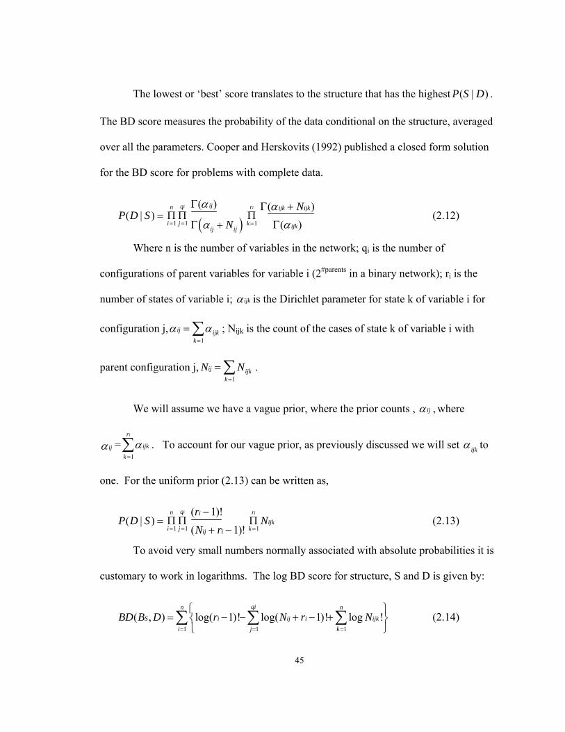
45
The lowest or ‘best’ score translates to the structure that has the highest P(S | D) .
The BD score measures the probability of the data conditional on the structure, averaged
over all the parameters. Cooper and Herskovits (1992) published a closed form solution
for the BD score for problems with complete data.
( | )P D S = Πi=1
nΠj=1
qi
( )( )ij
ij ijN
α
α
Γ
Γ +Πk=1
ri Γ(α ijk + Nijk)
Γ(α ijk) (2.12)
Where n is the number of variables in the network; qi is the number of
configurations of parent variables for variable i (2#parents in a binary network); ri is the
number of states of variable i; α ijk is the Dirichlet parameter for state k of variable i for
configuration j,α ij = α ijkk=1∑ ; Nijk is the count of the cases of state k of variable i with
parent configuration j, Nij = Nijkk=1∑ .
We will assume we have a vague prior, where the prior counts , α ij , where
α ij = α ijk
k=1
ri
∑ . To account for our vague prior, as previously discussed we will set α ijk to
one. For the uniform prior (2.13) can be written as,
( | )P D S = Πi=1
nΠj=1
qi (ri −1)!
(Nij + ri −1)!Πk=1
ri
Nijk (2.13)
To avoid very small numbers normally associated with absolute probabilities it is
customary to work in logarithms. The log BD score for structure, S and D is given by:
1 1 1( , ) log( 1)! log( 1)! log !
qin n
S i ij i ijki j k
BD B D r N r N= = =
⎧ ⎫= − − + − +⎨ ⎬
⎩ ⎭∑ ∑ ∑ (2.14)

46
To illustrate the BD, consider the Smoking to Bronchitis network. This network
consisted of binary variables with associated counts as shown in Table 2.4. Each node
can be assigned a score corresponding to its having no parents. For the Bronchitis node
B, this no-parent score is given by,
(9!)(11!)(21!)
2.835 ×10⁻⁷
If we add an arc to the Bronchitis node with Smoking as the parent, the score is,
(6!)(4!)(11!)
⎛⎝⎜
⎞⎠⎟
(3!)(7!)(11!)
⎛⎝⎜
⎞⎠⎟= 3.28 ×10⁻⁷
The ratio of the two posterior probabilities is:
P(S1 | D)P(S2 | D)
=2.835 ×10⁻⁷
3.28 ×10−7 = 0.864
Therefore, if the structures have equal prior probabilities then the posterior
probabilities satisfy the P(S1, D) = 0.864P(S2 , D) . The posterior probability of S2 is
higher than the posterior probability of S1, thus supporting an arc from Smoking to
Bronchitis. The higher score for S2 means that the data provides evidence a relationship
existing between Smoking to Bronchitis in the manner indicated by the graph.
Generally, the most common process is to use a greedy search to find structures
with high scores. However, greedy algorithms can become stuck in local minima and
stop. The K2 algorithm developed by Cooper and Herskovits (1992) uses a greedy
search for finding a network structure. The algorithm is very effective for learning

47
network structures from data but the draw back is two fold. First, the algorithm requires
node ordering; second, the data must be complete.
This dissertation considers an extension of Myers’ PopMCMC algorithm that
employs BD scoring. As previously noted, the PopMCMC method developed by Myers
has the added benefit of not requiring knowledge of the node order. PopMCMC uses
statistical information from a population of Metropolis-Hastings samplers to select and
modify a population of individual structures. The process of modifying the structures
continues until a stopping criterion is met. The structure with the best BD score among
the sampled structures is selected. In this paper it is assumed that node order is not
known.
In summary, learning BN structure can be broken down into three components,
the scoring metric, which is used to grade how well the network fits the data; the search
of the proposed networks for the best; and the method for inferring the parameters of the
network. Most of the algorithms for learning structure operate similarly: they begin with
a structure, propose changes, and compare the posterior probabilities of the two
structures. The ‘greedy’ deterministic algorithms keep the structure with the highest
score, whereas, the stochastic algorithms can escape local minima but they can also
accept change that makes the score worse. The process continues until a stopping
criterion is met.
2.4. Learning Bayesian Networks with Continuous Variables
Many of the machine learning algorithms are not designed to handle numeric
attributes, especially commercially available software [Clarke and Barton, 00, Dougherty,

48
et al., 95, Kohavi and Sahami, 96, Friedman and Goldszmidt, 96]. Most commonly
available BN software requires the variable to be discrete. According to Cartlett (1991),
discretization of data can speed up learning because the learning process can handle
nominal better than numerical attributes. Similarly, Monti (1999) concluded from his
experiments that learning BN structure was improved with discretized data as a
preprocessing step. However, as we have noted previously, many real world datasets
contain continuous variables. The process of transforming numerical continuous
variables into discrete variables requires the variables’ data to be partitioned.
Numerous methods for discretizing have been developed over the years.
Dougherty, et al (1995), and later Kohavi and Sahami (1996) provided a general
overview of discretization techniques. The discretization methods can be divided into
two categorical groups: supervised vs. unsupervised; and global vs. local [Dougherty et
al., 95; Kohavi and Sahmi, 96]. The categories can be further divided into hierarchical or
nonhierarchical methods. These five dichotomies can be shown in a hierarchical
framework with the associated discretization methods. Figure 2.5 shows this framework.

49
Figure 2.5. Hierarchical framework of discretization methods.
Discretization
Bottom
-Up
Top-D
own
Supervised
Unsupervised
Supervised
Unsupervised
Global
Local
ChiM
ergeC
hi2
None
Global
LocalG
lobalLocal
D2
1R
K-m
eans
Clustering
Adaptive
Quantizer
Equal W
idthE
qual Freq
Discretization
Bottom
-Up
Top-D
own
Supervised
Unsupervised
Supervised
Unsupervised
Global
(Static)
Local
ChiM
ergeC
hi2
None
Global
(Static)
Local(D
ynamic)
Global
(Static)
Local
D2
1R
K-m
eans
Clustering
Adaptive
Quantizer
Equal W
idthE
qual Freq
ID3
Discretization
Bottom
-Up
Top-D
own
Supervised
Unsupervised
Supervised
Unsupervised
Global
Local
ChiM
ergeC
hi2
None
Global
LocalG
lobalLocal
D2
1R
K-m
eans
Clustering
Adaptive
Quantizer
Equal W
idthE
qual Freq
Discretization
Bottom
-Up
Top-D
own
Supervised
Unsupervised
Supervised
Unsupervised
Global
(Static)
Local
ChiM
ergeC
hi2
None
Global
(Static)
Local(D
ynamic)
Global
(Static)
Local
D2
1R
K-m
eans
Clustering
Adaptive
Quantizer
Equal W
idthE
qual Freq
ID3

50
2.4.1 Unsupervised discretization methods
Unsupervised discretization methods partition a variable based on a distribution of
the values of the variables. There are several commonly used methods; one of the
simplest methods in this category is equal-width intervals, in which the sorted data is
divided into a specified number of intervals with equal number of data points in each
interval. The user specifies the number of k intervals. The interval width, d is found
as: d = ( Xmax − Xmin ) / k , where Xmax the maximum value is bounded and Xmin is the
minimum value bounded. The bins are found by: Xmin + i(d) , where i=1,2,…,k-1. A
similar method is equal frequency, which divides the data into intervals with equal
numbers of observations.
Another type of unsupervised method attempts to find natural clusters in the data.
These clusters define the discretization. A common clustering method is the k-means
method [Bradley and Fayyad, 98, Everitt, et al, 01]. This method is from a family of
iterative clustering methods. For the k-means method the data is divided into a pre-
specified number of non-overlapping groups or clusters. The mean of the cluster is the
reference point. The mean can be adjusted during and after each partition. The distance
from a data point to the mean is measured as squared distance for means and absolute
distance for medians [Weiss and Indurkhya, 95]. The k-number of clusters is pre-
established. The process of moving data points continues until a convergence condition
is met or the standard deviation is minimized for each cluster.
Several authors have found in empirical studies that unsupervised discretization
methods do not perform as well in terms of classification accuracy as supervised

51
discretization methods [Dougherty et al, 95; Monti and Cooper, 99; Clarke and Barton,
00, Liu et al., 02]. The unsupervised methods are more arbitrary in the division of the
data points. The user generally predetermines the number of k-partitions. The attractive
feature of unsupervised methods is their simplicity, especially if the user only wants
quick resolution. They are also used when there is not any information to determine
relationships between variables. The disadvantage is these methods ignore classes and
labels to divide the data [Lam and Low, 00, Liu et al. 02]. This can result in over
partitioning of the data as well as division of relevant groups. It also gives equal
treatment to outliers that can skew the true distribution [Cartlett, 91].
2.4.2 Supervised discretization methods
Supervised discretization techniques are used to discretize features used in a
classification problem. They seek to maximize a measure of the relationship between the
features and the class. The ChiMerge [Kerber, 92], Chi2 [Liu and Setiano, 95] and
StatDisc [Richeldi and Rossotto, 95] use statistical tests, similar to hierarchical clustering
techniques. For most of the statistical techniques, the data is first sorted then partitioned.
The algorithm of choice merges the adjacent intervals in a bottom-up process with some
predetermined level of significance, α, in place for termination. The user determines the
level of significance. If only one state or interval is left, it is declared ‘not relevant’
because one bin does not properly represent the data set [Kerber, 92].
The statistical methods mentioned for discretizing data are variations of the
ChiMerge. The partitions for the ChiMerge method are compared based on the chi
square independence test. The statistical test is,

52
χ 2 =(Aij − Eij )
2
Eijj=1
k
∑i=1
m
∑ (2.15)
Since only two intervals are compared, m=2, k represents the number of classes,
Aij are the number of examples in the ith interval in the jth class, and Eij is the expected
frequency where,
Eij =Ri ∗Cj
N, i=1,…m, j=1,…k (2.16)
N is the total number of examples where,
N = Cjj=1
k
∑ (2.17)
Cj is the number of examples in the jth class,
C j = Aiji=1
m
∑ , j=1,…k (2.18)
R is the number of examples in the ith class,
Ri = Aijj=1
k
∑ , i=1,…m (2.19)
The degrees of freedom is the number of classes minus one. The process works
as follows,
1. Place all data points into their own interval.
2. An alpha or level of significance is set to a high value, such as 0.5.
The above formula (2.17) for the χ 2 is used to determine whether an
interval should be merged or not merged. The intervals below the
threshold are merged.

53
3. Check whether a termination criterion is met. Is so, exit. If not, return
to step 2.
The past 15 years has seen a significant rise in the number papers employing
entropy discretization methods. Methods such as entropy, information gain, or MDL
measure the strength of a relationship based on information theory [Cartlett, 91; Fayyad
and Irani, 93; Dougherty, et al, 95; Friedman and Goldszmidt, 96; Kohavi and Sahami,
96; Clarke and Barton, 00].
Entropy, commonly denoted by H(X), is used to measure the amount of
uncertainty associated with a random variable, (X) or event. The information required to
describe the random variable is measured in bits. The entropy or information of a
discrete random variable can be viewed as a measurement of the expected amount of
information concerning the variable. If we want to know the outcome of a coin flip,
initially we do not know if it will be heads or tails. Each of the two outcomes, (x) have
an associated probability (p). If we knew that the outcome was heads, then there would
be no uncertainty and H(X) would be zero. The information associated with the
probability distribution is measured as:
H (X) = − p(x)log2∑ p(x) (2.20)
Entropy-based methods minimize the amount of uncertainty associated with an
outcome. In most cases, entropy based methods used for discretization of continuous
attributes are minimization heuristics. Algorithms such as ID3 and C4.5 are entropy
based discretization methods originally developed for decision tree problems. Methods

54
developed by Catlett (1991) and later by Fayyad and Irani, (1993) are an extension of
those earlier works. The process developed by Fayyad and Irani has been extended and
employed in various discretization methods [Friedman and Goldszmidt, 96; Dougherty, et
al, 95]. The entropy method basically looks for binary partitions for each attribute.
One such method is called the minimal entropy partitioning method [Dougherty,
et al, 95]. It is a supervised algorithm that uses class information entropy to determine
the partitions. For the minimal entropy partitioning the algorithm is designed to
minimize the entropy function for the possible partitions. The algorithm is based on the
following equation:
E(A,T ,;S) =| S1 || S |
Ent(S1) +| S2 || S |
Ent(S2) (2.21)
The above notation closely follows that of Fayyad and Irani as sited by
Dougherty, et al (1995). Notationally, A represents a given feature, T is the boundary
which minimizes the entropy function over all the possible partition points and is taken to
be the ‘best’ boundary point; S is a set of instances or attributes that determines the
binary discretization boundary. It is calculated for all candidate partitions, TA. The
binary partition for A is the partition point TA for which E(A,T;S) is minimal among all
candidates. This method described is an iterative, top-down process. The partitioning
process continues until a stopping criterion is met. A common criterion to determine
when to stop is the Minimal Descriptive Length (MDL) Principle.

55
Monti used a multivariate discretization method with a latent variable to improve
the discretization process [Monti, 99]. This method, similar to those discussed in this
section, discretizes the data as a preprocessing step to learning the BN structure. The
process uses a latent or hidden variable to determine the relationship between variables.
The relationships are scored using a Bayesian scoring metric, which is based on the MDL
principle. The variables are discretized based on the highest score given a fixed structure
and observed data.
Another multivariate method for discretizing continuous variables is called the
Derivative Method (DM) [Brown, 03]. The Derivative Method measures the amount of
change in a data set. The data points are ordered. An estimate of the derivative is
calculated at each point, excluding the first point. The variable X has the values 1, , nx x…
and the variable Y has the values 1, , ny y… . The derivative is estimated at each point,
using the approximation,
1 1 1 1( ) / ( )ii i i i
dy y y x xdx + − + −≈ − − , i=2,…(n-1) (2.22)
and
1 1( ) / ( )ii i i i
dy y y x xdx − −≈ − −
for i=n. The first cut point is established at i=1. Taking the absolute value, the
total amount of change measured is summed up and divided by the number of bins. The
total amount of change is
2_
ni
i
dytotal change dx=
=∑ (2.23)

56
The number of bins is determined by the user. The term ‘bins’ is interchangeable
throughout this paper with partitions and cut points. The next step in discretization is to
calculate the cut points for each variable. The width of the cut point is determined by
finding the point that does not exceed the threshold set as the total amount of change for
each bin. The amount of change for each bin is: change per bin=total change/#bins.
This process is repeated until all cut points for the two variables are found. The
process can be applied to the more difficult problem for multiple continuous variables
with continuous parents or children and for continuous variables with discrete parents or
children. Multiple continuous variables that are related by arcs are discretized
simultaneously. The root nodes are identified and the data for each root node’s
continuous dependent children are sorted on the root node. A down side to the DM is it
requires all observations, which are not common for real-world data because some
observations could be missing.
The Markov Chain Monte Carlo Method using Bayesian Dirichlet (BD) score is a
heuristic search and score method that uses the Metropolis-Hastings algorithm for
acceptance and rejection of the proposed discretization based on the BD score of the
candidate cut point. A modification to the search method allows the process to split or
merge intervals [Xu, 03]. The process starts with an ordered data set and a maximum
number of bins as set by the user. Every pair of data points constitutes an interval. Each
continuous node is then discretized in an iterative method by randomly selecting a cut
point, score the change and either split or merge bins to improve the BD score. The
process for splitting or merging bins is done randomly based on a probability set by the

57
user. For splitting, the bin is divided into two bins. Conversely, the merging process
merges the right side of the interval into one bin. The end points of the data set are
excluded for either splitting or merging. The process of search and scoring continues
until all continuous nodes are discretized over a specified number of iterations.
The Hill Climbing (HC) method with BD score is the last method to be used in
this study [Xu, 03]. The HC method is also a search method that attempts to improve the
overall score by incrementally changing the cut points. The process begins with ordered
data sets for the continuous variables and a set of initial cut points. The incremental
process searches for improvements to the BD score until the user defined number of cut
points for the continuous node is achieved. Unlike the traditional HC, this HC method
loops through the search process twice. The first loop randomly selects a cut point to
evaluate. Cut points are evaluated one at a time while the others remain fixed. If the
change improves the score it is accepted otherwise no change. The changes are proposed
randomly to avoid being stuck in local optima. The second loop repeats the process in an
attempt to improve the score.
2.4.3 Global vs. local discretization methods
The cluster analysis method by Chmielewski and Grzymala-Busse (1994) is also
sometimes called a mixed supervised/unsupervised method. It can also be classified as
global or local. The authors viewed the clustering phase as global while the fusing of
adjacent intervals as local. Local discretization methods are applied to one variable at a
time such as the k-means clustering and the hierarchical maximum entropy methods.

58
Global methods are applied to all the variables as a preprocessing step to learning.
Each continuous variable is discretized independent of the other attributes. The variable
has Πi=1n ki regions, where ki is the number of partitions of the ith feature. Methods that
are considered global include the ChiMerge, equal width intervals, equal frequency
intervals, as well as 1RD [Holte, 93] and D-2 [Catlett, 91]. The last two methods are
based on dividing the continuous variables into pure class bins. The first method passes
only one time through the data the later passes through twice.
2.4.4 Outcomes of experiments
Two key papers on discretization of continuous variables set the standard of
comparison for discretization research. A paper by Dougherty, Kohavi and Sahami
(1995) did the first comprehensive analysis of various types of discretization techniques.
They then conducted in depth experiments on three methods: the equal width interval,
1RD (Holte) and Entropy minimization heuristic, based on Fayyad and Irani (1993). The
three methods were used with the Naïve Bayesian (NB) classifier.
The Naïve Bayesian classifier is a very effective and popular classification
method [Dougherty, et al, 95, Friedman & Goldszmidt, 96]. The purpose of the NB is to
accurately predict the class of the test group when class information is included. It
assumes all feature variables are independent conditioned on the class variable. The NB
is commonly used as the ‘gold standard’ when testing other classifiers. This does not
mean that the NB is without error but it does provide a useful standard of comparison for
the performance for classifiers. The NB computes the posterior probabilities of the

59
classes given the data. The features are assumed independent for each class. Discrete
variable probabilities are based on counts and continuous variable probabilities are based
on a Gaussian distribution. Therefore, comparing discretization methods used as
preprocessing steps to the NB classifier provides a common base for comparison.
The results from Dougherty et al. concluded that the minimal entropy partitioning
method for discretizing continuous variables classification performance was better than
the other two methods. They also concluded that the supervised global entropy-based
discretization improved the accuracy of the induction algorithm better than unsupervised
global method (equal width interval).
Friedman and Goldszmidt (1996) drew similar conclusions concerning global
minimal entropy partitioning. They tested three unsupervised methods for learning
discretization and structure of the network. The first method was the least squares
clustering method. The discretization is initialized with k = log2 Ni , where k is the
number of partitions for the lower bound. The upper bound was set at five partitions.
Where Ni ≤ 32 for the partitioning of the variables. The other two methods were
variations on minimal entropy partitioning. One was done as a preprocessing method
(Fayyad and Irani’s method), the other was applied with the NB classifier. The latter was
global in that it discretized variables that were independently taking into account only the
class variable. This results in computing only the information gain for each possible new
proposed partition. The network was discretization and then learned using a greedy
search algorithm.

60
Friedman and Goldszmidt concluded from their tests that discretization using
MDL captures variable interaction with adjacent variables sufficiently well for learning
BN structure. The non-interacting variables were discretized in isolation. Their results
for discretization showed that MDL performed just as well as the class-based
discretization method used by Fayyad and Irani. They also applied their discretization
policy to learning a BN. Their iterative process only found local minima and terminated
after three iterations. They concluded that the choice of initial discretization could affect
the BN.
Recently published papers have built upon previous methods for discretizing
continuous variables for learning Bayesian Network [Monti, 99; Clarke and Barton, 00;
and Lam and Low, 00]. The first author examined two basic discretization methods:
quantiles (50% and 33% quantiles) and the k-means clustering technique [Chmielewski
& Grzymala-Busse, 94]. The cluster and quantiles methods were both tested using the
Bayesian Dirichlet scoring metric. The cluster method was also tested using the MDL
scoring metric. The last test employed quantiles as a preprocessing step and then learned
the structure from the discretized variables. The result of the tests showed that the cluster
and quantiles using BD metric outperformed the other two methods significantly in terms
of structural accuracy of the learned BN models [Monti, 99].
Clarke and Barton (00) in their experiment used two discretization methods: an
entropy based discretization method for discretizing the data and an equal interval
method. They tested their processes first using the MDL scoring metric and then the BD
scoring metric. The entropy based discretization method out performed the equal width

61
partitioning method based on the strength of conditional dependencies in the data. The
results were based on using the MDL scoring metric. They also applied the MDL to a
method they called dynamic repartitioning. Their method applied the MDL metric to first
find the best discretization policy. The nodes were partially ordered with the continuous
variables as the parent nodes and scored the results using the BD metric. They did not
have significant improvement over the pre-partitioning process using their dynamic
process. Additionally, based on the process described in their paper and attempts to
obtain the algorithm the process for dynamic repartitioning is not available to replicate.
Lam and Low (2000) tested three methods for discretization and then used two
methods to learn the Bayesian networks. They examined equal partitioning method,
using an algorithm due to Lloyd [Lloyd, 82], a clustering method, and the entropy
minimization method. Similarly as in the previous two papers, the equal width method
did not perform as well as the other methods. Their tests resulted in Lloyd’s algorithm
performing the best based on the F-measure which is a weighted utility score.
The various discretization methods examined by previous authors discussed
[Monti, 99; Clarke and Barton, 00; and Lam and Low, 00] discretized one variable at a
time. In cases involving hidden variables, the feature variable may not be known and
therefore class-based discretization is not always the best method. One of the goals of
this work is to learn BNs based on the interaction among all the variables. The desired
approach in our study is to do a global discretization as oppose to discretizing one
variable at a time. Discretizing one variable at a time might obscure or create spurious
relationships among the variables.

62
Additionally, the discretization methods discussed used various methods as a
preprocessing step to learning a network. The one paper that used a method called
dynamic repartitioning did not have significant improvement over their entropy method
as a preprocessing step. There is not, to our knowledge a process for discretizing
continuous variables that successfully interleaves the discretization with learning.
2.5 Missing data and hidden variables
Missing data is common with real world datasets. There are numerous reasons
data may be missing. Information may be missing due to error or oversight, as when a
survey respondent accidentally fails to enter a response to a question. Information may be
missing due to unavailability of the unit of observation, as when a patient in a medical
study has died or moved away. Information may also be missing due to intentional
withholding of information, as when a participant in a drug rehabilitation program is
unwilling to answer questions on his or her progress due to embarrassment or fear of
negative repercussions. The methods used in this study assume the data is missing at
random (MAR). The following definition of MAR comes from Allison (2001). If there
are only two variables X and Y, where X is always observed and Y sometimes is missing,
the data are missing at random if,
P(Y_missing |Y,X)=P(Y_missing |X)
Missing data could also be categorized as missing completely at random
(MCAR). The data is MCAR if the data on Y is unrelated to the value of Y or the values
of any other variable in the dataset [Allison, 01]. For example, if we had a survey to
examine consumer spending the data would be considered missing at random if the

63
probability of non-response did not depend on the spending pattern (big or small spender)
that would have been observed. It would be missing completely at random if non-
response was equally likely for any categories that could be constructed from the other
variables (e.g., college graduates versus non-college graduates, etc.).
The discretization methods previously described are appropriate when the data are
complete, there are no hidden variables, and all variables are discrete. However, real
world data often has missing data as well as hidden variables. These types of problems
are the most difficult for structure learning. There is no closed form expression for
calculating the posterior distribution. If a new variable were introduced into the data then
the possible number of structures to enumerate would increase exponentially causing the
marginal likelihood calculations to be intractable. [Binder, et al., 97; Cooper, 95;
Murphy, 01].
Table 2.7 shows a classification of BN learning methods due to [Murphy, 01].
Learning problems are categorized according to whether the structure is known or
unknown, and whether data are complete or incomplete.
Table 2.7. Contingency table for classifying learning methods.[Murphy, 01]
Structure Complete/Observable-fully Incomplete/Observable-partial
Known Closed form Expectation Maximization (EM)/MCMC
Unknown Local search Structural EM/MCMC

64
The most difficult category is learning when the structure is unknown and data are
incomplete or hidden. For this kind of problem, estimating the parameters is very
difficult because there is no closed form solution for the relative probabilities of
structures. Such problems are common in the medical field. For example, there are
situations in medicine, which the disease is not known but the symptoms are visible.
When the disease is not known then all the observed symptoms appear related. As
another example from the medical domain, a Bayesian network with hidden and visible
variables for Black Death might look like Figure 2.6.
Figure 2.6. A Bayesian Network with Plague as hidden variable.
The structure on the left shows the nodes interconnected with the parent nodes
and all the symptoms. The insertion of the hidden variable, plague disconnects the
structure and simplifies the network, making learning much easier. As with the plague,
there are many times when the disease is not known and the symptom variables are not
Plague
Pain in lymph nodes
Headache Internal bleeding
Pain in lymph nodes
Headache Internal bleeding
Patient Information
Hidden Disease
(no observations available)
Symptoms
B CA B CA
Plague
Headache Internal bleeding
Pain in lymph nodes
Headache Internal bleeding
Patient Information
Hidden Disease
(no observations available)
Symptoms
B CA B CA B CA B CA
Plague
Pain in lymph nodes
Headache Internal bleeding
Pain in lymph nodes
Headache Internal bleeding
Patient Information
Hidden Disease
(no observations available)
Symptoms
B CA B CA B CA B CA
Plague
Headache Internal bleeding
Pain in lymph nodes
Headache Internal bleeding
Patient Information
Hidden Disease
(no observations available)
Symptoms
B CA B CA B CA B CA B CA B CA

65
observed directly. These problems complicate learning the structure of the network.
Several authors have concluded that an expert could be used to create smaller structures
as with the case in the figure above. However, this is not practical for large problems and
there are cases in which use of experts is not practical or no expert is available.
Two approaches for estimating the parameters of a BN when there is missing data
are the Expectation Maximization (EM) and Markov Chain Monte Carlo (MCMC)
methods. The EM is a general-purpose method for statistical parameter estimation. It is
generally used to calculate maximum likelihood estimates of parameters in problems with
incomplete data. EM is an iterative method for finding a posterior mode of the likelihood
function. The EM algorithm has two parts: the E and the M steps.
To see how EM works, consider random variables drawn from a distribution with
the density f(D|θ), where θ represents the parameters of the model and D represents the
complete data. We let X be the set of hidden variables and Y the set of observed
variables. We write D=(X,Y) to represent the observed and unobserved random
variables. We use lowercase letters d=(x,y) to denote a specific realization of the random
variable D=(X,Y). We define,
Q(θ |θ ( i) ) = E[log P(x, y |θ) |θ ( i) , y) (2.24)
Where θ( i) is the ith iteration of EM and the (i+1)th iteration is calculated in two
steps. That is, Q(θ| θ(i)) is the expected value of the log-likelihood. In other words, we
do not know the complete data, so we cannot say what is the exact value of the
likelihood, but given the data that we do know (the x's), we can find a posteriori estimates
of the probabilities for the various values of the unknown y's. For each set of y's there is

66
a likelihood value for θ, and we can thus calculate an expected value of the likelihood
with the given values of x's (and which depends on the previously assumed value of θ
because this influenced the probabilities of the y's) [Gilks, et al, 96].
The steps of the EM algorithm are as follows from Gilks, et al (1996),
1. The E-step: Compute Q(θ |θ ( i) ) .
2. M-step: Update θ ( i) by computing the maximizer of . Q(θ |θ ( i) )
The process of maximizing the posterior distribution using the parameters, or
sufficient statistics continues until convergence.
The structural EM [Friedman, 98] combines a greedy search process over
structures with the EM algorithm for estimating the parameters. The EM algorithm may
get stuck at local minima. Therefore, the common practice is to use multiple starting
points to avoid getting stuck.
Another method for treating missing data is Markov Chain Monte Carlo
(MCMC). MCMC is a general purpose stochastic search method used for optimization
and inference. The most commonly applied MCMC method is the Metropolis- Hastings
algorithm, of which Gibbs sampling is a special case [Gilks, et al., 96].
Bayesian Dirichlet scoring, combined with MCMC works well for complex
problems such as the one discussed above, when there is no closed form solution due to
missing data and hidden variables. In these cases it is not computationally feasible to
find the exact BN parameters. It has been noted that the M-H algorithm has a theoretical
advantage because the stationary distribution is chosen by design [Laskey, 02].
Therefore, MCMC provides an approximation to the posterior distribution of the

67
parameters. However, the traditional M-H sampler can be slow, whereas the PopMCMC
converges more quickly, as will be discussed in the next section of this paper.
2.6 Discretization and learning
Two structure learning methods will be discussed in this section, Population
Markov Chain Monte Carlo (PopMCMC) [Myer, 99] and Belief Network Power
Constructor (BNPC) [Cheng, 97]. Both of these methods will be used to learn BNs from
discretized data in our study.
2.6.1 Population Markov Chain Monte Carlo (PopMCMC) method
Population Markov Chain Monte Carlo (PopMCMC) is one of a class of
stochastic search algorithms that are useful for difficult search problems. The
PopMCMC is a canonical MCMC algorithm [Neal, 93] that uses a population of
Metropolis-Hastings samplers. This approach designs the Metropolis-Hastings algorithm
to sample over the missing observations and fill-in the missing values. If the data is
assumed to be ‘missing at random’ then the posterior distribution is proportional to P(X,
Y|S)P(S), where X is the observed data, Y is the filled-in missing values and S is the
structure. This distribution can be calculated in closed form for any structure [Laskey &
Myers, 03].
The M-H algorithm can be applied to a variety of difficult optimization and
search problems. It can be applied to any optimization problem in which the objective
function can be computed for any two candidate solutions up to a multiplicative constant.
It can also be used for inference problems in which the probability ratio can be computed
for any two proposed solutions.

68
In MCMC the process samples from a stochastic process with a unique stationary
distribution. Samples from an MCMC process can be used to obtain estimates for the
expectation of the stationary distribution. Usually a burn-in sample is discarded and
estimates are based on observations taken after burn-in.
MCMC sampling works as follows. The process works by modifying the current
realization X = {X1,..., Xn} of the process. A random change to X is recommended and
either accepted or rejected. The distribution of Xn given Xn−1 is called the transition
distribution. If the transition distribution does not depend on n, then the chain is said to
have a time-invariant transition distribution. If the transition distribution is time-invariant
and all states are reachable from all other states then the chain has a unique stationary
distribution [Feller, 68]. A chain satisfies detailed balance if:
π (x)T (x, x*) = π (x*)T (x*, x) (2.25)
where T(x,x*) is the probability of transitioning from X=x to x=x*.
If (2.27) is satisfied, then the distribution �(x) is a stationary distribution.
In M-H sampling, the changes are accepted or rejected depending on the ratio of
the target and proposed density. The proposed state, xp is picked at random from a
proposal distribution, S(x,xp). The proposed state is accepted with probability A(x,xp).
The next state x* is equal to x if xp is rejected and xp if xp is accepted. In this case, the
transition distribution can be written as:
T (x, x*) = S(x, x*)A(x, x*) (2.26)
if x≠x*. The acceptance probability for the M-H algorithm is,

69
A(x,x*) = min
p(x*)q(x | x*)p(x)q(x* | x)
,1⎧⎨⎩
⎫⎬⎭
(2.27)
where q(x*|x) is the proposal distribution. The acceptance rule works by generating a random number, u from a uniform
distribution [0,1), and setting the next state according to,
x* =x p ,x,
⎧⎨⎩
u < A(x, x p )otherwise
It is possible that the chain will remain in the same state for many iterations. The
move is based on an acceptance probability. The new move is more likely to be accepted
when there is a high value for the test ratio. If the value is low for the test ratio the move
is more likely to be rejected. Also, if the Markov chain ‘mixes well’ it tends to transition
the parameter space quickly and converge to the equilibrium distribution. If the chain
does not ‘mix well’ the moves are small and can take many iterations to converge.
The approach taken in the PopMCMC to learn BNs from incomplete data is to use
two Markov chains and sample from the two proposal distributions simultaneously: one
to sample for the incomplete data, the other for the BN structure. Let S1 denote the
proposal distribution for incomplete data and let S2 denote the proposal distribution for
structures. The log BD score is used to evaluate the structures.
The PopMCMC algorithm proceeds as follows:
1. Generate an initial population of solutions, where a solution consists of
a BN structure and values for the missing data.
2. Score the solutions using the BD scoring metric.

70
3. Use the population of solutions to estimate parameters for the proposal
distribution for both arcs and missing data.
a. Randomly select a structure and values for the missing data.
b. Add, delete, or reverse arcs according to the structure proposal
distribution.
c. Randomly modify missing data values based on the missing data
proposal distribution.
4. Compare BD scores for the old and new structures and missing data
values.
5. Accept the proposed new structure and missing data values using the
M-H acceptance rule. If not accepted, retain the old solution.
6. Continue until the stopping criterion is met (number of iterations set
by the user).
The strength of the PopMCMC method is that the samplers use global information
about the population of solutions. The benefits are two fold: it increases the rate of
convergence and improves efficiency of the sampler. The PopMCMC algorithm is a
statistical search method that also produces a population of ‘good’ solutions as oppose to
one ‘best’ solution. Useful statistical inference can then be drawn from the population of
structures.
A solution we are pursuing is to use PopMCMC to produce the population of
solutions and interleave the discretization with learning. Myers demonstrated a slight

71
benefit in multiple models for learning structure [Myers, 99]. We hypothesize that
sampling from the multiple models should produce better results.
2.6.2 Belief Network Power Constructor (BNPC) method
The second structure learning method used in this study is Belief Network Power
Constructor (BNPC) [Cheng, 97]. BNPC is freely available via the Internet. The BNPC
can be categorized as a Conditional Independence (CI) test algorithm as opposed to a
search and scoring algorithm. Similar to PopMCMC the BNPC algorithm does not
require node order but does require the variables to be discrete. However, it assumes
there is no missing data. It also assumes the data are sampled independently given the
underlying probabilistic model of the data. The dataset must also be large enough for the
CI tests to evaluate the data but BNPC will only use the first 100 cases in the data set.
The algorithm for learning BN is an extension of a tree construction algorithm [Chow and
Liu, 68].
BNPC employs two algorithms: One for when the ordering is known and the
other when ordering is not known. The algorithms employ Conditional Independence
(CI) tests. The algorithm takes the database as input and constructs a belief network as
the output. The output can remain as a text file or be exported to one of three belief net
software packages to perform inference: Hugin net format of Hugin Expert A/S, Netica
format of Norsys Software Corp and Bayesian Interchange Format version 0.15.
The process followed by BNPC has three phases: drafting, thickening and
thinning. The first phase is drafting. The drafting phase computes the conditional mutual
information for pairs of nodes. The mutual information of two nodes is defined as:
72
( Xi , X j ) = P(xi
xi ,x j
∑ ,x j ) logP(xi ,x j )
P(xi )P(x j ) (2.28)
The conditional mutual information is defined as:
( Xi , X j | C) = P(xi
xi ,x j ,C∑ ,x j ,c) log
P(xi ,x j | c)P(xi | c)P(x j | c)
, where C is the set of nodes.
The output is a singly connected graph without loops. Algorithm A primarily
uses the Chow-Liu algorithm for this phase to construct the tree. The Chow-Liu
algorithm is incorporated into the first phase and is based on dependence analysis using
information theory. In this phase, the algorithm looks for closeness between two nodes
as a measure of mutual information. By using pair-wise mutual information test result
(CI tests are not used) the nodes are put into a list from highest to the lowest scores.
Then arcs are added and re-scored; if the score is below a threshold the node is removed
from the list. The process, or ‘draft phase’ as called by the authors, stops when an open
path in the acyclic graph has expressed every pair-wise dependency.
Phase two of Algorithm A is called thickening. The steps in this procedure
require the algorithm to “try_to_separate” nodes, in which each node is examined to
determine if it can be d-separated. Both d-separation and CI tests are conducted on a set
of nodes to determine if the nodes should be connected or not. Edges are added if the set
of nodes cannot be separated.
The final phase is called thinning. A procedure called “find_cut_set” is used to
find a cut-set that can be d-separated in the newly formed graph. Since the order of the
nodes is known it is possible to determine if the node is a collider or a non-collider.
Colliders are nodes in which two arcs meet head to head (or collide at their heads). Then

73
the process of finding a cut-set that can be d-separated is simplified. In the final phase
the algorithm revaluates the relationships in order to remove all wrongly added arcs and
thin the graph. The thinning and cutting of the algorithm is based on Pearl’s definition of
perfect map [Pearl, 88].
Figure 2.7. A simple multi-connected network
The main difference between the two algorithms is Algorithm B does not need
node ordering to learn a structure. The three phases are the same as those of Algorithm
A, drafting, thickening and thinning. The difference is in phase III.
The purpose of Phase III is to lessen the chance of incorrect edges by rechecking the
edges that connect a pair of nodes. Both algorithms use the procedure of
“try_to_separate” to evaluate if nodes can be separated. However, the B Algorithm
(A) (B)
(C) (D)
A B
D
C
EA B
D
C
E
A B
D
C
E A B
D
C
E

74
evaluates a group of nodes instead of pairs in the Markov blanket. For example consider
the structure shown in Figure 2.8.
Figure 2.8. Connected structure learned by BNPC.
The decision rule to remove edges states: If all paths of the underlying model M
can be closed between two nodes, then accept the paths connecting two nodes by one
collider [Cheng, et al., 97]. For example, Figure 4 would examine {A,B,C,D} as the
group. Nodes X and Y would be separated.
The process described does not always orient the edges correctly due to the
limited ability to identify colliders. If the model has more edges and more colliders the
algorithm performs better. Two well-known examples the authors use are the ALARM
and the Asia networks. In the ALARM network 42 out of 46 edges were correctly
oriented and no extra edges were incorrectly added. By contrast, the Asia network, out of
the eight nodes one edge was missing and two edges were miss-oriented. The errors are
due to the dependency not being strong enough for the algorithm to find the edges.
2.7 BRAC background
X A Y
BC
D

75
The case study for this dissertation is a data set from the Base Realignment and
Closure (BRAC) process. BRAC was created out of a need to reduce the number of
bases the Department of Defense had amassed from World War II and Korea. After the
war, there was a force reduction, but no reduction in the number of bases. By the 1960’s,
the Department of Defense recognized the need to reduce the number of bases.
In discussing the BRAC process, it is important to distinguish between base
closure and base disposal. Base closure or realignment means the mission of an
installation has been transferred or ceased. The disposal of an installation or base means
the ownership of the land and facilities has been transferred to a private or public
organization1.
The BRAC process began in the 1960s under the Kennedy administration. Then
Secretary of Defense, Robert McNamara was directed to develop and implement an
extensive plan to realign and reduce bases and installations held by all services. Under
his direction, DOD was able to close 60 bases. The successful closure of the bases was
because there was no Congressional oversight or involvement. This was the last time
bases were closed without Congressional involvement. Because government bases and
installations have economic and political ramifications to their states, Congress has
become involved in all subsequent base closure decisions.
Congressional involvement in bases closures was signed into law under the Carter
administration in 1977. The law mandated Congressional approval for any closure or
disposal of bases. However, the process came to a standstill and no bases were closed
1 Throughout this paper a base or installation will be understood to mean the same thing

76
until Congress passed two laws in 1988. The first law was the Base Realignment and
Closure Act, which recommended the closure of 125 major military installations and 225
minor military bases for all services. The second law established a nonpartisan,
independent commission to study the bases proposed for closure. The committee for the
1988 BRAC rounds recommended to the Secretary of Defense closing 97 bases and
realigning 55 bases and installations. Despite these recommendations, no bases were
closed or realigned during the 1980s due to political deadlock in Congress.
In 1990 another law was passed to reduce political interference in base closure
and realignment. The law required DOD to provide the commission with a list of
proposed bases based on a force structure plan and budget requirements. Unlike the
proceeding years, Congress and the administration concurred that there was a need to
reduce defense budgets due to a changing world order. Specifically, the Cold War had
ended with the fall of the Berlin Wall in 1989 and the dissolution of the Warsaw Pact in
1991. Congress was looking for an opportunity to sharply reduce defense spending.
These events lead to a decrease in the military forces, across all services by
approximately 25% over the next 5 years [BRAC 1993 Report to the President].
Even though there was a strong need to reduce base holdings, after 4 base closure
rounds [1988, 1991, 1993 and 1995] only 60% of the Army’s total acreage has been
reduced taking an average of 8.2 years. This amount only represents less than 10% of the
total acreage (258,946) the Army has scheduled for disposal. Table 2.8 shows the total
acreage per round.

77
Table 2.8. BRAC round acreage and time to disposal by percentage [Harris et al., 04].
BRAC Round
Total BRAC Acreage
Years for 60% Disposal
Years for 80% Disposal
Base Closure Acreage Drivers
1988 87,997 12 12 Jefferson Proving Grounds (50,385)
1991 34,535 15 23 Two Ft. Ord parcels (14,773) 1993 2,664 6 6 Tooele Army Depot (1,621) 1995 133,750 8 8 Sierra Army Depot (57,633)
In terms of Army installations, there has been minimal success in meeting the set
requirements for time. Historical records show that out of the 71 installations approved
for closure only 12 have closed in three years or less and only 34 have been disposed of
in 6 years or less. Table 2.9 shows the installation numbers and percentage by rounds.
Table 2.9. BRAC round installation closure and disposal times [Harris, et. al. 04]
BRAC round
No. of Installations
No. closed in 3 yrs
% of total installation by round
Median Closure Time
No. Disposed in 6 yrs
% of total installations by round
1988 28 0 0% 5.59 12 43% 1991 6 0 0% 3.80 3 50% 1993 4 1 25% 4.10 2 50% 1995 33 11 33% 3.45 17 52% Cumulative 71 12 17% 4.38 34 48% The 2005 BRAC guidance the Army Basing Study (TABS) office wants to
decrease the time to close and dispose of installations. The directive establishes two
goals: to close or realign 60% of the 2005 installations within three years or less; and to

78
achieve disposition of 60% of the bases in six years or less. The reduced time to dispose
of bases has an economic consequence. The longer a base takes to close the greater the
cost in terms of resources and money such as $3.5 billion in environmental costs.
Conversely, early closure can be a tremendous cost savings. The closure of bases thus far
has resulted in $16.7 billion in savings [GAO report 05-614, 05].
The process of closing and disposing of bases is a difficult and complex process.
Issues such as environmental cleanup have been a major obstacle with base dispositions
and a source of uncertainty. This had been due to several factors that make cleanup
costly as well as time consuming. Disposition time is influenced by environmental
factors such as cleanup of unexploded ordnance, contaminated sites, ground water, etc.
The amount of time required to meet the EPA standards for a region creates uncertainties.
Because of this uncertainty, it is difficult to predict how long it will take to dispose of a
base. Additionally, the duration of cleanup can increase as environmental requirements
change.
Other issues that impact base closure include: the number of jurisdictions
surrounding the base; the amount of economic dependency by the community on a base;
the number of military retirees in the community; and number of acres of the base
[Lachman, et. al, 03]. These issues as well as others made it difficult for the Army’s
BRAC Office (BRACO) to accurately predict the amount of time to close or dispose of a
base. Several studies by both the General Accounting Office (GAO) and the Army
BRACO have identified issues that impacted the closure and disposition. The studies did
not determine how all these factors interact and influence the time for closure or disposal

79
of bases. The studies also did not provide a method to evaluate the amount of time to
close a base to obtain an accurate assessment.
The BRACO is responsible for closing and disposing of Army bases. Previously
they had used the amount of time to close a base as the main performance measure to
assess their success rate. Later, they used acreage as the primary measure. A recent
study [Harris, et. al, 04] found it difficult to use any one factor to accurately assess the
process. Additionally, the study through linear regression was unable to find any one
driver that impacted the disposal of a base. The study found that R2 were very low, as
shown in Table 2.10.

80
Table 2.10. Results of correlation of variables in the BRAC data [Harris, et. al, 04].
Hypothesis Data Analysis Finding The amount of environmental
cleanup lengthens the disposition time.
Actual Environmental Cost vs. Actual Disposition Time R2 = 0.02
The amount of environmental cleanup lengthens the disposition
time.
Estimated Environmental Cost vs. Actual Disposition
Time R2 = 0.01
As environmental cost increases, disposition cost increases.
Actual Environmental Cost vs. Total Cost to Disposition
R2 = 0.14 (after removing one outlier R2
increased to 0.32) The amount of MEC (UXO)
increases the disposition time. Actual MEC Acreage vs. Actual Disposition Time R2 = 0.12
The amount of MEC (UXO) increases the environmental cost.
Actual MEC Acreage vs. Actual Environmental Cost R2 = 0.87
Larger installations have longer disposition times.
Actual Acreage vs. Actual Disposition Time
R2 = 0.0037 (completed dispositions)
Installations with more square footage take longer to close.
Starting Square Footage Inventory vs. Actual Closure
Time
R2 = 0.07 (wrong hypothesis)
Some EPA Regions have longer disposition times.
EPA Region vs. Actual Disposition Time No sufficient correlation.
Some MACOMs have longer disposition times.
MACOM Owner vs. Actual Disposition Time
TRADOC Dispositions take less time than
others.
The type of installation impacts the closure time.
Installation Type vs. Actual Closure Time
Administrative and industrial installations
take longer to close than others.
The type of installation impacts the disposition time.
Installation Type vs. Actual Disposition Time
Family housing locations are quicker to dispose than other installation
types. The type of installation impacts the
actual cost to disposition. Installation Type vs. Actual
Cost to Disposition Major training areas cost
more for disposal. Superfund sites have higher
environmental costs associated with them.
Superfund Site vs. Actual Environmental Cost
Superfund sites incur more environmental
costs.

81
The only strong correlation existed between the amount of unexploded ordnance
and environmental costs. They concluded that there was no single variable driving the
closure time, disposition time or costs [Harris, et. al. 04]. Additionally, they tried to
apply multi-variable regression analysis to the data but found it was inappropriate due to
the small sample size and missing data.
A common theme that is evident in all the studies reviewed [GAO, 98; BRACO,
01; Lachman, et. al, 01; Harris, et. al, 04] is that the disposition of a base is a complex
task. The task of developing methods to improve the process is difficult due to the
number of factors we listed. Additionally, the dataset on previous BRAC rounds is small
with mixed variables and missing data creating a difficult task to develop a linear
regression model for predictions. The TABS office would like a model that allows them
to perform evaluations and predictions on installation closures and dispositions. In the
next chapter we will lay out our proposal to develop a model to conduct inference on
disposition times through Bayesian networks.

82
3 Methodology
In this chapter, we present the experimental design we used to evaluate the
various hypotheses for our study. Principally, the design consists of a detailed approach
to interleaving discretization of continuous variables with the learning of structure in a
Bayesian Network.
This study’s global objective was to empirically study and test four hypotheses.
We evaluated interleaving discretization methods with the learning of structure in a
Bayesian Network. The challenge associated with learning Bayesian Networks becomes
more difficult when data are missing at random and structure is unknown [Friedman, 98].
A greater challenge is to learn structure from continuous variables with incomplete data.
We further extend our investigation to assess the performance of discretization in the
presence of missing data.
In addition, we applied our new methodology to actual data from the U.S. Army’s recent
Base Realignment and Closure (BRAC) study [Harris, et. al. 04]. This data set contains
both continuous and discrete variables and is complicated by missing data. Our goal was
to improve performance in terms of accuracy by better discretizing the continuous
variables. Accuracy can be improved by finding a discretization policy that avoids
information loss due to discretization. A desired outcome of our study was to minimize
the loss of information due to discretizing continuous variables. We then measured the

83
quality of discretization in terms of the BD score achieved through discretization
measured the quality of discretization in terms of the BD score achieved through
discretization.
This chapter is organized as follows. In the first four sections we present a
detailed explanation of the experimental hypotheses for this investigation, the testing
procedures designed to illuminate evidence in support or against these hypotheses, and
appropriate accompanying discussions meant to further illuminate the rationale
motivating their exploration. Following this, we describe the design for testing the
hypotheses for comparing the performance of the three discretization methods we applied
to continuous variables present in data. We next describe the experimental tests using the
two structure learning methods we used to interleave with the discretization methods.
We will also describe the performance metric used for each of the tests.
3.1 Hypothesis I
The first experimental hypothesis of this study was intended to test whether or not
identification and classification accuracy of learning of BN can be improved by
interleaving discretization and structure learning into the Bayesian Network: When
continuous variables are involved, interleaving discretization with learning of structure
will reduce the information loss due to discretization thus improving classification
performance.
Method:
We used two discretization methods and two structure learning methods for our
experiments (see Table 3.1). The discretization methods were Markov Chain Monte

84
Carlo (MCMC) [Gilks et al, 96] with BD score and Hill Climbing (HC) [Pearl, 85] with
BD score. The structure learning methods were PopMCMC and BN Power Constructor.
The discretization methods and PopMCMC are programmed using MATLAB, 6.5,
Release 13 [18 June 02]. The learning method, Power Constructor is programmed in C,
version 2.2 [Cheng and Bell, 98].
Table 3.1. Discretization and learning methods.
Discretization Method Learning Structure Method 1. MCMC with BD score 1. PopMCMC 2. Hill Climbing (HC) with BD score 2. BN Power Constructor
The various discretization methods interleaved with the learning algorithms were tested
to evaluate their relative predictive performance. To demonstrate this hypothesis we
tested the methods through a systematic process as shown in Figure 3.1.

85
Figure 3.1. Systematic approach to Hypothesis I.
Figure 3.1 shows the three types of comparisons we tested. The first comparison,
(A), compared discretization without interleaving with learning performed as a single
step, for each of the four combinations of discretization and learning methods. This
allowed us to infer whether there are measurable improvements as hypothesized.
The second comparison depicted (B), compared the four interleaved combinations to each
other. We wanted to determine which of the four discretization interleaved with learning
performs the best overall.
The final comparison, (C), was to examine the best results of discretizing
interleaving learning with non-interleaved learning from a previous study in which
structure was known [Xu, 03]. We desired to determine how close we could come when
(A) Against non-interleaved
learning
(C) Against previous results
(individual)
(B) Against each other

86
structure is not known, if any over previous results in which the structure was known.
The metrics used to evaluate the methods was the number of incorrect relationships based
on known structure.
Test:
The objective of the study was to test which interleaved combination from the
table above provides the most accurate inference in response to queries. The tests we
performed are described below. Results are described in the next chapter.
All discretization methods were evaluated on the same datasets. To evaluate the
different discretization and learning methods we examined how different factors
influence performance. We varied the different factors in our study within a range of
values we have set. Table 3.2 shows the various design factors we varied and the range
of values for each. In the case of algorithm selection the range is among four different
combinations of discretization with learning methods.
Table 3.2. Design factors.
Design Factors Description Values Number of continuous nodes
The number of continuous nodes in the dataset
Low: 1 High: 13
Number of discrete nodes The number of discrete nodes in the dataset
Low: 2 High: 35
Number of cut points User indicates number of cut points
Low: 2 High: 5
Percent of data missing Percentage of data missing from dataset
Low: 1% High: 30%
Algorithm selection The discretization and learning method
6 combinations

87
We conducted tests using data sets from University of California, Irvine (UCI)
repository of machine learning databases. This repository contains the most commonly
used sets in the literature on discretization of continuous variables. The data sets vary in
size and number of continuous nodes. We used a known solution as our ‘gold standard’
throughout the experiment to provide a base to examine various performance measures.
The ‘gold standard’ was the network created for sensor and fusion projects [Chang and
Laskey, 03], which has known structure and mixed variables. Additionally, we tested our
process against previous studies using the UCI datasets [Friedman, 98, Cheng, et al, 98].
We also used two known hypothetical problems found in the literature, the Alarm and
Asia networks. Our final dataset consisted of real world data from the four previous
BRAC rounds (1988 to 1995). Datasets used in this study are shown in Table 3.3.
Table 3.3. Datasets for design study.
Variables Dataset Continuous Discrete
Sensor and Fusion network (Chang and Laskey) 13 2 Iris (UCI repository) 4 0 Diabetes (UCI repository) 1 8 Alarm (Beinlich, et. al., 1989) 2 33 Asia (Lauritzen and Spiegelhalter, 1988) 1 7 BRAC (1988-1995) 29 9
We used the same measures of performance to examine all three proposed
comparisons and evaluate the results in a matrix format. The measurements of interest
are:

88
(i) The test of accuracy was based on classification accuracy of the learned
Bayesian Network (BN). The numbers of errors were assessed in two categories
for each method tested, the number of false positives and the number of false
negatives.
(ii) The second measure was the BD score that is the logarithm of the posterior
probability of the network given the data. The closer the BD score is to zero the
better the more likely or probable the network represents the data.
(iii) Logarithmic loss was used to measure how well the model predicts an
observation. The log( )
log cN Ploss
N−
= ∑ , where Pc is the probability
predicted for the correct state c; and N is the number of cases in the test set. For a
correct prediction P would equal 1 and zero would correspond to an incorrect
prediction. The log loss score is used to evaluate performance of the different
methods.
(iv) The last error test was the 2 2_ _ _ (1 )j c
j cquadratic loss score is p p
≠
= + −∑
It is similar to the log loss score but is between 0 and 2, with 0 being the best and
the spherical payoff is between 0 and 1 with one being the best. A low score for both the
log loss and quadratic indicates good performance.
The last test component was to examine how the learned network performs under
various scenarios and evaluate the outcomes. We varied the evidence variables, the
target variables and the values of the evidence variable. If the target variable was discrete
we examined the probability assigned to the correct hypothesis as measured by the log

89
loss and quadratic loss scores. If the target variable was continuous we used the
difference between the correct value and the assigned value using the mean squared error.
Additionally, another measure that could have been used is the Receiver Operating Curve
(ROC) to assess the performance of the various discretization methods. The ROC
graphically demonstrates the affects of discretization of the continuous variable that plot
of sensitivity (true-positive rate) verses specificity (false-positive rate) at all possible
thresholds. Measures such as true positive and true negative rates can be used to
determine the accuracy and predictive power for test data sets with BRAC historical data.
The posterior probability distribution was analyzed using the BD score to give us insights
into the quality of the BNs. We also compared the Best-so-far curves for the BD score
for the different methods. The curve is a plot of the score of the best solution found up to
a given iteration against the iteration number. The measures of performance are show in
Table 3.4.
Table 3.4. Performance measures.
Name Description 1 Error rate The percentage of wrong predicted number 2 ROC Area under curve show how well algorithm performs 3 Logarithmic loss Log loss values are calculated using natural log. Zero
indicates best performance. 4 Quadratic loss or Brier
score Is between 0 and 2, with 0 being best and spherical payoff is between 0 and 1 with 1 as best.
5 Confusion Matrix For each algorithm a matrix giving the predicted number of each state and the actual number.

90
Discussion:
Except as noted earlier, all other applied discretization processes discretize the data prior
to learning BN structure. The discretization is done as a preprocessing step to learning.
Creating partitions for the continuous variables prior to learning could result in defining
categories that do not accurately reflect the structural relationships among the variables.
This may result in less accurate inferences than if structural relationships were properly
accounted for. This research evaluated the hypothesis that interleaving the two processes,
thereby resulting in more accurate responses to queries, could reduce the amount of
inaccuracy or error.
3.2 Hypothesis II
Continuous variables with observations missing at random (MAR) can be
discretized successfully by combining a Monte Carlo method for filling in the missing
data with a stochastic search over discretization policies. Success is defined in terms of
the performance metrics discussed in Section 3.1.
Method:
The Monte Carlo method in PopMCMC was used to generate a population of
solutions for the missing data. The stochastic search method, using MCMC finds
partitions and then scores them based on the Bayesian Dirichlet (BD) score.
Test:
Data sets from UCI repository [Murphy and Aha, 95] were used to test the
performance of the MC method for filling in data. The data sets from the repository were
used to generate missing data sets. We generated the missing data by a process that

91
ensures the missing observations are missing at random. The data sets with missing data
allowed us to test the performance of our method.
Discussion:
The current methods for discretizing continuous variables exclude observations
that contain missing data. Our research found no algorithms, other than Laskey and Xu
that could perform discretization in the presence of missing data. However, many real
world datasets are comprised of continuous and discrete variables with missing data.
Therefore, there is a need for a method, which can discretize in the presence of missing
data.
3.3 Hypothesis III
The performance of a discretization algorithm has a measurable degradation as
the amount of missing data increases. Through empirical study we can determine the
relationship between performance and the amount of missing data.
Method:
As above, the Monte Carlo method in PopMCMC was used to generate a
population of solutions for the missing data. The stochastic search method, using MCMC
finds partitions and then scores them based on the Bayesian Dirichlet (BD) score. We
varied the percentage of missing observations to evaluate the dependence of algorithm
performance on the amount of missing data. We evaluated the results based on metrics
discussed previously.

92
Test:
Known data sets from UCI repository were used to test how well our method
performs in filling in the missing data for discretization. Taking the known data sets and
creating data sets with missing observations allowed us to test the impact on
performance. The randomly missing observations were systematically increased by
percentage of 1, 5 and 10% to empirically study the amount of degradation in
performance. We used the measures of performance (MOP) discussed to evaluate the
relationship.
Discussion:
When the amount of missing observations is relatively small relative to the total
sample size any adverse effects on the discretization policy should be negligible.
However, as the amount of missing at random (MAR) data increases we expected there to
be an adverse effect in the performance of the discretization policy. An empirical study
allowed us to measure the degradation in the relationship between performance of
discretization policies and the amount of missing data.
3.4 Hypothesis IV
When structure is unknown, and/or there is a relatively large amount of missing
data, Arc counts over multiple structures and discretization policies will result in more
accurate inferences than using a singe ‘best’ model.
Method:
Incorporating the Monte Carlo method for filling missing data and MCMC for
discretization, we hypothesized that PopMCMC would result in multiple models as set by

93
the user. We used a set of test data to determine if the models provide accurate inference
to queries. From the models produced we took a set number of the models produced to
conduct the arc counts.
Test:
There is a direct dependency between two nodes if there is an arc from the parent
node to the child node. To determine the most likely relationships between nodes we
conducted an arc count. For each dataset an arbitrary threshold was set for the number of
occurrences that an arc went to a node to determine the BN structure. As the final step,
we compared the results obtained in this test with the single models produced to see if
there was a significant improvement in our predicative capability.
Discussion:
When structure is not known we can learn structure from the data and based on a
metric select the model that maximizes the metric of choice such as BD, BIC, AIC and
MAP to name a few. However, when there is uncertainty associated with data in which
one model does not dominate over the others or is not overwhelmingly more probable,
selection of a single model may perform more poorly than averaging multiple models.
The cause of one structure not dominating over another may be due to several factors.
One factor could be that the data is questionable. If the data set is large and not
questionable it may still not provide enough information to distinguish between different
models. Therefore, more than one structure may be probable based on the uncertain data.
When several models have a high posterior probability, research suggests using model
averaging [Madigan, Raftery et al. 96. Friedman and Koller, 00, Neapolitan 04]. As has

94
been shown [Herskovits, 91, Madigan and Raftery, 94] model averaging may be
appropriate for certain cases to improve predictive capability. For cases in which
hypothesis that produced the data is unclear, model averaging may improve the predictive
performance over a single best model. We expected a statistically discernable
improvement from the use of arc counting over a single model.
We used the MCMC and Hill Climbing with BD scores for discretization. The
two methods for learning structure were PopMCMC and BN Power Constructor. The
various discretization methods interleaved with the learning algorithms were tested to
evaluate their relative predictive performance. The details of the methods employed for
discretization and learning are also discussed in greater detail in chapter 2.

95
4 Experiment
The purpose of this chapter is to discuss the outcome of the experiments devised
to evaluate the various hypotheses for our study. The principal focus of our study is on
the interleaving discretization of continuous variables with learning of structure in a
Bayesian Network. We evaluated our process using test cases and applied our
methodology to actual data from the Army’s Base Realignment and Closure (BRAC)
study. The experimental design was discussed in detail in the previous chapter.
This chapter is organized as follows. In the first section we present the software
implementation to support the experiments. The subsequent sections will address the
outcomes of the experiments for each of the hypotheses we proposed in the last chapter.
4.1 Software implementation
We integrated several software packages to allow us to conduct the
experiments proposed in Chapter 3. We required software to transform our data to a
format that was easily exportable to other packages. Therefore, the majority of the
software we selected for evaluating and supporting our process is available commercially
or is freely available for research use. The primary and supporting software programs we
used were Microsoft Excel for the database files, Netica ® and BNPC for constructing
Bayesian Networks and Matlab ® for interleaving discretization and learning. All four
software programs were incorporated into a single architecture to support our study.

96
The primary software we used to implement our process was Matlab7®. Matlab
is a high-level computer language available commercially and distributed by
Mathworks®. It is used by many universities including George Mason University.
Additionally, the programs we incorporated in our final package were originally written
in Matlab. Therefore to maintain the integrity of those programs we wrote the integration
software in the same program.
The program for interleaving discretization and learning BNs consists of two
main files. Each file contains several script files known as m-files. The files were kept
separate due to common naming issues with the files. To integrate the two files, a main
file was created along with subprograms to bridge the differences between the two
programs. The overall main program was required to allow interleaving of discretization
and learning without rewriting the previous code. The interleaved process requires an
initial structure. In order to learn an initial structure, the continuous variables in the data
set were discretized using equal width binning method. Then an initial structure was
learned using the PopMCMC algorithm. Once the initial structure is learned, the user
could choose a discretization method for the original data set. Then structure learning
program was applied again on the newly discretized data. The process is summarized as
follows for interleaving of discretization and learning structure.
Input database (i) Discretize with equal width binning (ii) Learn initial structure with PopMCMC (iii) Discretize using structure-based discretization algorithm
(a) Select search method (Hill Climbing and or MCMC) (b) Select scoring method (BD or MDL) (c) Select number of cutpoints and iterations (d) Output cutpoints with highest score

97
(iv) Repeat for a user-selected number of iterations: (a) Discretize again (prepares dataset for learning structure)
(1) User selects cutpoint method for data (2) Software places cutpoints into dataset
(b) Learn structure with PopMCMC (1) Discretized data loaded (2) Select number of iterations (3) Select number of parents (4) Select number of structures (5) List of n-structures and best structure based on BD score (6) Save best structure
(v) Output cutpoints and learned structure with the best score (vi) Export learned structure to Netica
The same process is used for BNPC structure learning as discussed above but
only for discretizing the dataset. After the cutpoints are learned for the dataset the
discretized dataset is imported into BNPC.
The Matlab process, after the initial discretization and structure are learned, saves
the structure with the highest BD scores among the structures enumerated during the
search. The user chooses the number of iterations for interleaving discretization and
learning. The process takes the best structure learned and attempts to improve the
cutpoints based on a chosen search method. The process iteratively takes the improved
cutpoints and new structures learned based on a chosen metric to update the best
structure. The final structure and dataset with the cutpoints are saved as files.
The databases used in our process were imported and exported to Microsoft Excel
files. This software was used to allow us to save the files in several versatile formats.
These formats allowed us the flexibility to move among the various programs employed
in our study. For each database, an Excel workbook was created allowing us to
consolidate our spreadsheets for evaluation and for building BNs.

98
The two software packages used to build the Bayesian Networks were Netica ®,
version 1.12 and Bayes Net Power Constructor created by Dr. Cheng from the University
of Alberta, Canada [Cheng et al., 97]. For our experiment we used both capabilities for
comparison to our proposed process. In order to establish a common means to evaluate
the networks the learned structures from PopMCMC and BNPC were exported to Netica.
Netica, produced by Norsys Software Corporation, is available as a limited free
ware or an unlimited commercial version. The software is versatile and flexible program
for building and learning Bayesian networks. It also allows the user to conduct various
tests on the networks with cases simulated or stored to evaluate the prediction capability
of the network.
The second software, Bayes Net Power Constructor for building BNs is free on-
line software that was discussed in detail in Chapter 2. The same process is used for
BNPC structure learning as discussed above but only for discretizing the dataset. After
the cutpoints are learned for the dataset the discretized database is imported from Excel
and constructs networks using CI tests. The software can build a BN with or without
node ordering. Once the relationships are learned the software allows the user to
automatically export the learned structure to Netica.
4.2 Hypotheses testing
The established architecture allowed us to evaluate our hypotheses using the
preexisting datasets. All of the datasets, except for BRAC are considered benchmark
data sets. The datasets we used are shown in Table 4.1.

99
Table 4.1. Datasets for design of study.
Variables Dataset Continuous Discrete Sensor and Fusion network (Chang and Laskey)
13 2
Alarm (modified) 22 33 Asia (modified) 13 7 Iris (UCI repository) 4 0 Diabetes (UCI repository) 1 8 BRAC 29 9
The methods discussed in Chapter 3 were tested using the data sets listed in Table
4.1. Three of the data sets had known structure: Sensor and Fusion, Alarm and Asia.
These data sets were tested initially to help validate the process we propose. The data
sets from the UCI repository have known attributes for each of the continuous variables
but not a known structure. Detailed information on the UCI data sets can be found at:
http://www.ics.uci.edu/~mlearn/databases/. The BRAC data does not have known
attributes for each of the variables or known structure. Additionally, only the BRAC data
set has missing data, see appendix A.
The datasets for the hypothetical medical problems, Asia and Alarm, are available
through Netica’s library. Both original networks have only discrete nodes. In the Asia
network, also known as Chest Clinic, we changed the smoking node to continuous based
on a study on lung cancer and tobacco consumption [Schairer and Schoniger, 01]. For 2 Nodes in dataset were originally discrete. Discrete nodes were modified to be continuous. Modification discussed later in the chapter 3 Node in dataset was originally discrete. Discrete note was modified to be continuous. Modification discussed later in the chapter.

100
the Alarm dataset we changed two nodes to continuous: blood pressure and heart rate.
The blood pressure ranges and probabilities came from the American Heart Association
and the heart rate ranges were obtained from Vaughn’s blood pressure website [Vaughn,
04]. The data tables were changed in Netica from discrete to continuous and 500 cases
were generated using Netica’s case-generation facility.
4.2.1 Hypothesis I: When continuous variables are involved, interleaving discretization
with learning of structure will reduce the information loss due to discretization thus
improving classification performance.
In the first phase the data with known structure was used to test how well
discretization without interleaving with learning performed as a single step. For each of
the known structure data sets we applied the learning algorithms using the settings shown
in Table 4.2 below. The number of parents for the initial data was set at the limit of the
true number of parents in the network. The experiment settings are as follows:
Table 4.2. Software settings for initial data run without interleaving.
Discretization Learning Structure Equal
width bins
Num Nodes
Num Continuous
Internal Iterations
Split Prob
Internal Iterations
Num Parents
Num Structures
Asia 4 8 1 10 .6 100 3 10 Alarm 4 37 2 10 .6 100 5 10 Sensor 4 15 13 10 .6 100 3 10
The software settings for the discretization of the continuous variables were based
on previous experiments conducted that found there were less than nine cuts, on average

101
when using the MCBD method. In our experiments we also found the number of unique
cutpoints learned was less than the set threshold of ten. The software for finding the
cutpoints for the continuous variables has a total of six discretization methods available.
In a previous study the author found that the MCBD performed the best (Xu, 03). We
concluded the same after a series of tests. The other discretization policies available are
listed in Table 4.3.
Table 4.3. Discretization policies.
Discretization Method Scoring Method Hill Climbing Bayesian Dirichlet Markov Chain Monte Carlo Bayesian Dirichlet Hill Climbing Minimal Description Length Markov Chain Monte Carlo Minimal Description Length Original Hill Climbing Bayesian Dirichlet Original Hill Climbing Minimal Description Length
Discretization independent of structure learning:
In the first comparison of our study we discretized the continuous variables
independent of the structure learning. This established a benchmark to allow us to infer
whether if there was any measurable improvement. For each of the three data sets 500
cases were generated with 50 holdout samples for testing. The results of the initial test
for Asia are shown in Table 4.4.

102
Table 4.4 Results of cutpoints for Asia data set.
True cutpoints
MCBD Score=-2.3150
HCBD Score=-2.2717
Non Smoker 0 0.905 0.9950 Light 1-5 0.975 9.675 Moderate 6-10 5.56 9.925 Heavy 11 or more 9.66 10.23
The structure learned in the single step was compared to the known structure. We
found the discretization without interleaving learning resulted in a structure that did not
properly represent the data. The results of our tests are shown in Table 4.5 below.
Table 4.5 Results of interleaving learning versus single step.
Dataset Interleaved with learning
structure BD score Not interleaved (single step)
BD score Asia -1.3521 -2.3150 Alarm -8.8940 -9.0842 Sensor -5.7131 -6.2186
The evaluation was based on comparing the known structure to the learned
structure. The learned structure had only one correct arc. Figure 4.1 and Figure 4.2
shows the known structure and the learned structure for both Asia and Sensor.
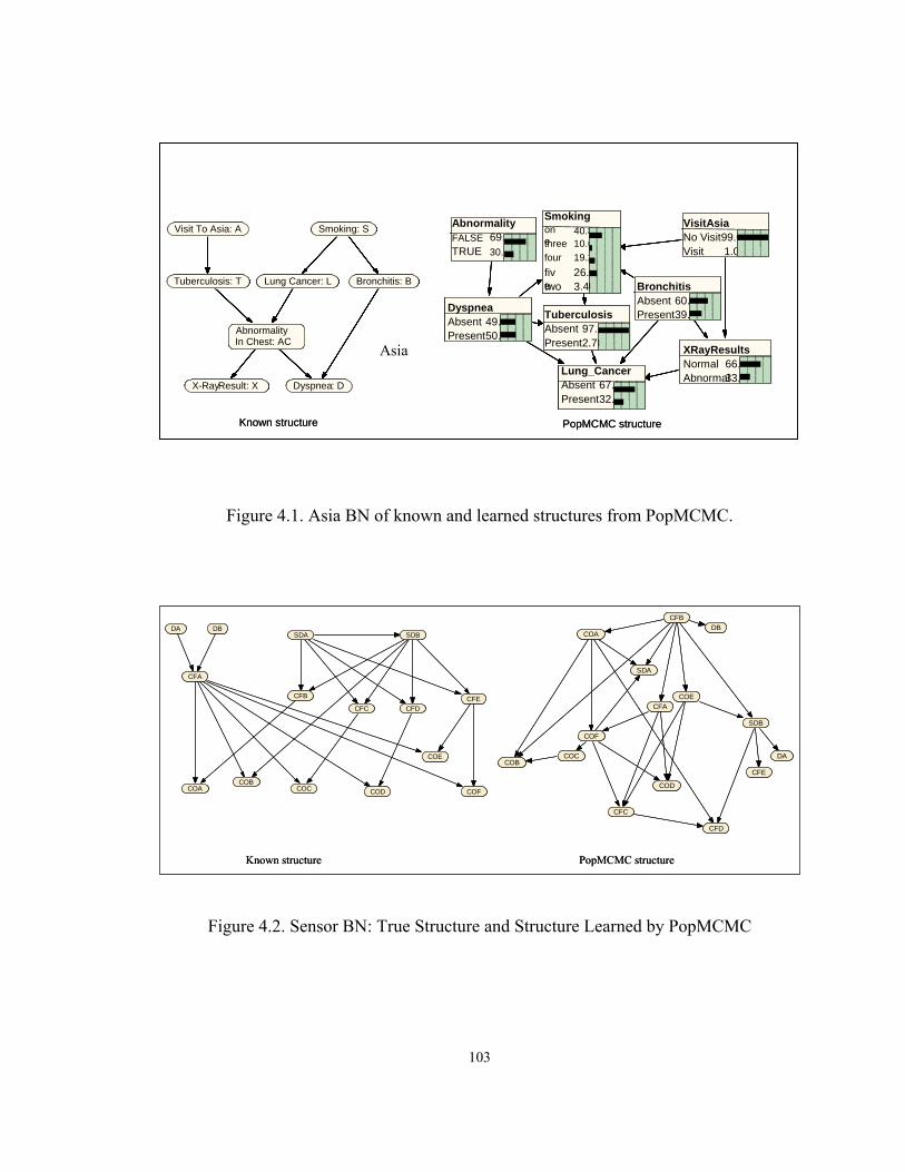
103
Figure 4.1. Asia BN of known and learned structures from PopMCMC.
Figure 4.2. Sensor BN: True Structure and Structure Learned by PopMCMC
AbnormalityFALSETRUE
69.130.9
VisitAsiaNo VisitVisit
99.01.0
BronchitisAbsentPresent
60.639.4
Smokingonethreefourfivetwo
40.810.619.226.03.46
Dyspnea49.650.4
Tuberculosis97.32.72
Lung_Cancer
AbsentPresent
67.932.1
XRayResultsNormalAbnormal
66.733.3
AbsentPresent
PresentAbsent
Tuberculosisor Cancer: TC
Lung Cancer: L Bronchitis: B
Smoking: S
Dyspnea: DX-RayResult: X
Tuberculosis: T
Visit To Asia: A
AsiaAbnormalityIn Chest: AC
Lung Cancer: L Bronchitis: B
Smoking: S
Dyspnea: DX-Ray Result: X
Tuberculosis: T
Visit To Asia: A
Asia
Known structure PopMCMC structure
AbnormalityFALSETRUE
69.130.9
VisitAsiaNo VisitVisit
99.01.0
BronchitisAbsentPresent
60.639.4
Smokingonethreefourfivetwo
40.810.619.226.03.46
Dyspnea49.650.4
Tuberculosis97.32.72
Lung_Cancer
AbsentPresent
67.932.1
XRayResultsNormalAbnormal
66.733.3
AbsentPresent
PresentAbsent
Tuberculosisor Cancer: TC
Lung Cancer: L Bronchitis: B
Smoking: S
Dyspnea: DX-RayResult: X
Tuberculosis: T
Visit To Asia: A
AsiaAbnormalityIn Chest: AC
Lung Cancer: L Bronchitis: B
Smoking: S
Dyspnea: DX-Ray Result: X
Tuberculosis: T
Visit To Asia: A
Asia
AbnormalityFALSETRUE
69.130.9
VisitAsiaNo VisitVisit
99.01.0
BronchitisAbsentPresent
60.639.4
Smokingonethreefourfivetwo
40.810.619.226.03.46
Dyspnea49.650.4
Tuberculosis97.32.72
Lung_Cancer
AbsentPresent
67.932.1
XRayResultsNormalAbnormal
66.733.3
AbsentPresent
PresentAbsent
AbnormalityFALSETRUE
69.130.9
VisitAsiaNo VisitVisit
99.01.0
BronchitisAbsentPresent
60.639.4
Smokingonethreefourfivetwo
40.810.619.226.03.46
Dyspnea49.650.4
Tuberculosis97.32.72
Lung_Cancer
AbsentPresent
67.932.1
XRayResultsNormalAbnormal
66.733.3
AbsentPresent
PresentAbsent
Tuberculosisor Cancer: TC
Lung Cancer: L Bronchitis: B
Smoking: S
Dyspnea: DX-RayResult: X
Tuberculosis: T
Visit To Asia: A
AsiaAbnormalityIn Chest: AC
Lung Cancer: L Bronchitis: B
Smoking: S
Dyspnea: DX-Ray Result: X
Tuberculosis: T
Visit To Asia: A
AsiaTuberculosisor Cancer: TC
Lung Cancer: L Bronchitis: B
Smoking: S
Dyspnea: DX-RayResult: X
Tuberculosis: T
Visit To Asia: A
AsiaAbnormalityIn Chest: AC
Lung Cancer: L Bronchitis: B
Smoking: S
Dyspnea: DX-Ray Result: X
Tuberculosis: T
Visit To Asia: A
Asia
Known structure PopMCMC structure
CFD
CFC
COE
DA
SDB
CFE
COD
COF
COB
COA
CFB
SDA
COC
CFA
DB
CFB
SDA SDB
CFC CFD
COA COD COF
COE
CFE
CFA
DBDA
COCCOB
PopMCMC structureKnown structure
CFD
CFC
COE
DA
SDB
CFE
COD
COF
COB
COA
CFB
SDA
COC
CFA
DB
CFB
SDA SDB
CFC CFD
COA COD COF
COE
CFE
CFA
DBDA
COCCOB
PopMCMC structureKnown structure

104
The one time discretization and learning was evaluated using two metrics, the
number of incorrect arcs or edges between nodes and the BD score associated with the
structure. These metrics were used to evaluate the two methods for learning structure,
PopMCMC and BNPC for each dataset. The arc error count is defined as follows. If
there is an arc incorrectly links two nodes when none should have been added, the arc is
counted as an error. Similarly, if an arc correctly links two nodes but is reversed in its
direction, it is counted as an error. Also, the arc is considered missing if the learned
structure does not have an arc connecting two nodes when there should be an arc. The
number of correct arcs is the number of arcs that correctly mimic the true structure.
The learning method BNPC allows for undirected arcs whereas PopMCMC does
not. In order to evaluate the BNPC structure learned with undirected arcs we randomized
the direction of the arcs based on a uniform distribution, left for 0 and right for 1. For
each structure with undirected arcs we created three sets of directed structures. Each time
the randomized method was used to create a structure with all arcs directed. This allowed
us to compute a BD score based on the average of the three structures.
Additionally, PopMCMC selects the best structure based on the Bayesian
Dirichlet score (BD). The BNPC uses a CI test to evaluate the arc relationships between
nodes but the software provides no score. Therefore, to evaluate BNPC we developed a
program to separately score the network learned by BNPC and generate a BD score. We
report the average of the three structures’ BD score as the overall score. Three sets were
selected due to small variation in score between the structures. This allowed us to
compare the two learned structures using a common metric.

105
We also scored the known structures of the three databases to create a ‘true’ BD
score as a base. The score of the known structures was used to compare to that of the
learned ones. We show the results of the ‘true’ structure scores in Table 4.6.
Table 4.6. ‘True’ network structure BD scores.
Network Name BD Score Asia -1.5630 Alarm -5.4735 Sensor -9.6244
The subsequent tables show the how each method performed for each dataset with
discretization done independent of learning (Tables 4.7 a and b).
Table 4.7a. BN structure learned using PopMCMC method.
PopMCMC Name # True Arcs # Error Arcs # Correct
Arcs # Missing
Arcs BD Score
Asia 8 11 1 0 -1.5922 Alarm 45 91 4 0 -8.8403 Sensor 23 21 5 0 -5.8695

106
Table 4.7b. BN structure learned using BNPC method.
BNPC Name # True
Arcs # Error Arcs
# Correct Arcs
# Missing Arcs
# Undirected Arcs
BD Score
Asia 8 1 5 2 2 -1.593 Alarm 45 10 7 0 32 -5.6827 Sensor 23 12 10 0 10 -9.3301
The initial baseline for the two programs was set by discretizing the data once
using MCBD process and then learning a structure. In comparing the BD scores of the
two learning algorithms to the ‘true’ score, both methods for the Asia network produce a
score very similar to the ‘true’ score. PopMCMC’s score for the three datasets had
varying results. The score for the Alarm dataset was the worse based on the true
structure and the score for Sensor was only a slight improvement. Whereas, BNPC’s
scores closely mimic the ‘true’ scores for all three datasets.
Two of the three datasets, Asia and Alarm were modified to add continuous
variables as previously discussed. The Asia network is the simplest of the three networks
tested with only one continuous variable. The results indicate no statistically significant
difference between the two learning algorithms for discretizing without interleaving
learning, similar to the results shown in Tables 4.7a and b. On the remaining datasets,
PopMCMC performed better than BNPC for the Sensor dataset whereas BNPC had a
better BD score for the Alarm dataset.

107
However, in terms of correct arcs BNPC consistently learned more correct arcs as
compared to PopMCMC. For the Asia dataset, PopMCMC found one correct arc
compared to BNPC’s five correct arcs. The BNPC would have performed better if we
count the undirected arcs with the correct node relationships as correct arcs. In the case
of the Asia network, the two undirected arcs would increase the count of correct arcs to 7
out of 8. There was no relationship found between the node Visit to Asia and any other
node in the network due to its extreme weakness as measured by the CI [Cheng, 98]. The
other missing arc was the one from Smoking to Bronchitis. The arcs from Bronchitis
were both undirected as indicated by the bold arrows. The modified BN is shown in
Figure 4.3.
Figure 4.3. BNPC modified learned structure for Asia data.
The inability of the learning algorithms, PopMCMC and BNPC to find the
dependency between the nodes Visit to Asia and Tuberculosis is due to the low number
Smokingxx1x2x3x4
45.02.9710.717.024.4
Dyspnea48.251.8
Bronchitis60.539.5
Lung Cancer
ABSENTPRESENT
68.331.7
XRay
ABNORMALNORMAL 34.4
65.6
AbnormalityTRUEFALSE
32.167.9
TuberculosisABSENTPRESENT
98.71.30 PRESENT
ABSENT
PRESENTABSENT
BNPC modified learned structure
Smokingxx1x2x3x4
45.02.9710.717.024.4
Dyspnea48.251.8
Bronchitis60.539.5
Lung Cancer
ABSENTPRESENT
68.331.7
XRay
ABNORMALNORMAL 34.4
65.6
AbnormalityTRUEFALSE
32.167.9
TuberculosisABSENTPRESENT
98.71.30 PRESENT
ABSENT
PRESENTABSENT
BNPC modified learned structure

108
of cases in which the Visit to Asia is positive. The limited number of positive responses
to Visit to Asia, one percent does not provide sufficient number of samples to indicate a
strong relation with Tuberculosis. We could have created an extension of the
mythological medical problem by which we increase the number of cases to generate a
larger number of positive Visit to Asia responses. This would have allowed us to
evaluate the relationship between Visit to Asia and Tuberculosis with the increased
occurrence of positive Visit to Asia. We could then conduct inference on contracting
Tuberculosis with the increased sample size. In this study we only note that the
insufficient sample creates a weak relationship between the two variables resulting in the
learning algorithms inability to find an arc between them.
The number of correct arcs for the Alarm network would also increase from 7 to
35 if the undirected arcs were added to the correct arc tally. However, for the Sensor and
Fusion network (Sensor) this is not case. There are 15 nodes in the network with 13
continuous nodes. The algorithm BNPC found 10 correct arcs. If undirected arcs with
correct relationships were counted this would only increase the count of correct arcs by
two.
Additionally, we evaluated the learned structures in Netica. The learned
structures from PopMCMC and BNPC for each of the datasets were exported to Netica.
Netica allows the user to test the network using cases. There were 50 test cases out of the
500 samples generated for each of the three datasets. To test the network starting with
Asia, all the nodes were selected and assumed to be unobserved. The software generates
beliefs for each of the unobserved nodes, in this case eight nodes. It then compares the

109
true value with the generated value and creates a summary statistics on the evaluation.
We used the scoring rule results to compare the two learning methods. The scores are
logarithmic loss, quadratic loss and spherical payoff. Recall the logarithmic and
quadratic loss scores provide a means to evaluate how well the model predicts. The
closer the scores are to zero the better predication accuracy. Similarly, the spherical
payoff ranges from zero to one with one being the best model performance. The scoring
methods were discussed in detail in the last chapter.
The BNs learned by BNPC required modifications in order to export and evaluate
using Netica. Any undirected arcs had to be edited prior to exporting to Netica. In the
case of missing arcs the node was left independent of all the other nodes. The undirected
arcs were directed using the method previously discussed for the BNPC. Netica provides
scores for each node in the network as part of the evaluation of the network. The scores
listed are an average of the results. The results for each method are shown in Table 4.8.
Table 4.8. Scoring rule result averages from Netica.
Scoring Rule Results Dataset Method Logarithmic Quadratic Spherical Payoff Asia PopMCMC 0.5850 0.3750 0.7784
BNPC 0.4754 0.3289 0.8109 Alarm PopMCMC 0.5327 0.2906 0.8335
BNPC 0.5211 0.2866 0.8389 Sensor PopMCMC 1.4604 0.7053 0.5300
BNPC 1.5409 0.7292 0.5118

110
BNPC performed slightly better than PopMCMC in the scoring metrics for two of
the three datasets, Asia and Alarm. However, as the number of continuous variables
increased the performance for both learning algorithms decreased. The Quadratic score
increased to 0.7 and the spherical payoff decreased to approximately 0.5. This could be
due to the one time discretization run used for learning the structure. The resulting
discretization did not have the benefit of learning a discretization policy based on a
correct structure. Results from a previous study [Xu, 03] demonstrated for a select few
datasets that the MCBD discretization is accurate if there is known structure to learn the
discretization policy.
The equal width method for discretization was also applied to compare with the
one time pass for discretization and learning. It performed as poorly, and in most cases
worse than the Markov Chain Monte Carlo with BD score. The equal width method is
sensitive to the number of intervals selected for the data and can create boundaries or
intervals where none should exist. In our test we initiated the process with four intervals
for one run. The number of errors is shown in Table 4.9. Both PopMCMC and BNPC
were used to learn structures.

111
Table 4.9. Comparison using equal width bins with PopMCMC and BNPC.
Equal width
PopMCMC
# Error Arcs
# Correct Arcs
# Missing Arcs
# Undirected Arcs
BD Score
Asia 10 3 0 N/A -1.3493 Alarm 85 4 1 N/A -9.2157 Sensor 26 1 0 N/A -6.2186 Equal width
BNPC
# Error Arcs
# Correct Arcs
# Missing Arcs
# Undirected Arcs
BD Score
Asia 4 0 0 9 -1.5522 Alarm 15 25 0 13 -1.1813 Sensor 6 9 0 3 -1.5249
There was only one instance for the Asia dataset, in which the equal width
method used with PopMCMC learning process performed better than the BNPC. The
learning algorithm, BNPC uses the Chi square test and found a greater number of correct
relationships, compared to PopMCMC. A possible reason for the improved performance
of the BNPC over the PopMCMC is the latter is slower but has shown to converge to a
better structure as the number of iterations increases. We show the improved
performance with increased iterations later in this study. We conjectured that the
interleaving of a discretization policy with learning would improve our learning of
Bayesian Networks. Previous research has shown that supervised discretization is better
than uninformed methods for learning structure [Monti, 99; Liu et al, 00].
Interleaving structure learning and discretization:

112
In the next phase we took the same datasets and we evaluated the results of
interleaving of structural learning with discretization. This was tested on datasets first
without missing data and then with missing data. For each of the datasets the iterative
process of learning and discretizing was run for 10 cycles (one cycle is defined as
discretizing with structure learning) with 100 internal iterations in PopMCMC. Each
dataset consisted of 500 cases with no missing data. After initial tests, we used the
MCBD discretization policy with the parameters set as shown in the previous Table 4.2.
The PopMCMC BD score for the datasets Asia and Sensor is better than the score for the
BNPC structures. Only for Alarm did BNPC perform better than PopMCMC as shown in
Tables 4.10a and b.
Table 4.10a. PopMCMC interleaved structure with discretization results.
PopMCMC Name # True Arcs # Error Arcs # Correct
Arcs # Missing
Arcs BD Score
Asia 8 12 2 0 -1.3521 Alarm 45 85 9 0 -8.8940 Sensor 23 25 4 0 -5.7131
Table 4.10b. BNPC interleaved structure with discretization results.
BNPC
Name # True Arcs
# Error Arcs
# Undirected
Arcs
# Correct Arcs
# Missing Arcs
BD Score
Asia 8 2 0 5 1 -1.5722 Alarm 45 10 32 8 0 -5.5431 Sensor 23 6 4 8 2 -9.6814

113
The number of error arcs and correct arcs does not significantly change for
either program. The number of error arcs for PopMCMC remains fairly constant in the
two tests (equal width and MCBD discretization with learning). The number of correct
arcs increases slightly for the Alarm, from 4 to 9 and for Sensor, from 1 to 4. In contrast,
BNPC improves for the dataset Asia with 5 correct arcs compared to zero for the equal
width test. However, for the other two datasets, Alarm and Sensor, BNPC decreases in
the number of correct arcs, increases in the number of undirected arcs and slightly
decreases the error count (see Table 4.10a and b).
The last tests we for interleaving discretization with learning of structure
was conducted on the datasets Iris and Diabetes (listed in Table 4.1). Both datasets are
from the UC Irvine machine learning data repository [Merz and Murphy, 96]. The
datasets were selected because of their repeated use in discretization and learning studies
[Dougherty et al., 95; Friedman and Goldszmidt, 1996; Liu et al, 02]. The Iris and
Diabetes datasets do not have known structure but they allowed us to test the learned
networks’ ability to accurately predict classification on small datasets.
The Iris data we used has 150 cases with no missing data. The data has
measurements, in centimeters of four flower parts: sepal length, sepal width, petal length
and petal width. The iris data has 50 specimens from each of three species: Iris setosa
(IS), Iris versicolor (IV) and Iris virginica (Ivir). There are a total of five attributes, four
continuous for the flower measurements and one nominal for the flower species. We ran
the data through our process for 10 cycles with 100 iterations each time in PopMCMC
and one time through BNPC. We had 10 holdout cases to conduct learning with cases in

114
Netica. As part of the evaluation of learning we randomly selected different
configurations of the holdout data four times.
The Fisher’s iris data, as it is commonly referred to, is often used for testing
classification accuracy. We used a classification graph for the iris data created by
MathWorks® to assist us in testing our predictions. Figure 4.4 shows the plot of the
data’s two sepal measurements in which the shapes are color coded to distinguish the
three species. Sepal width in on the y-axis and Sepal length is on the x-axis.
Figure 4.4. Iris species based on sepal length and width.
We evaluated our process of interleaving structure learning with discretization in
Netica. Since there is no known structure for the iris data we used Figure 4.3 to enter
evidence into our learned structure in Netica to evaluate our structure’s prediction
capabilities. We entered evidence on the sepal width and length as known. For example,

115
if we assume we knew the sepal width (SW) is large and its length (SL) is short we would
expect the model to predict, with a high probability that the type of iris species to be iris
setosa (IS). We entered the finding based on the graph clustering of species and found
our model to accurately predict the correct species. Figure 4.5 shows our learned
network.
Figure 4.5. Netica network of Fisher’s iris data.
The network in Figure 4.5 shows that there is a 77.7% probability the species is IS
based on the evidence entered. If we test the accuracy to predict the other two species we
find the following:
SLshortmedlong
10000
PLsmallmedlargeMLExlg
76.79.187.962.443.69
TypeISIVIVIR
77.713.58.86
PWsmallmedlargeExlg
72.214.07.755.98
SWExlglargesmallmed
0100
00
SLshortmedlong
10000
PLsmallmedlargeMLExlg
76.79.187.962.443.69
TypeISIVIVIR
77.713.58.86
PWsmallmedlargeExlg
72.214.07.755.98
SWExlglargesmallmed
0100
00

116
Table 4.11. Probabilities of species based on measurements.
Measurements Species SL SW IS IV IVIR
Short Exlg 84.6 10.3 5.02 Short large 77.7 13.5 8.86 Short small 45.2 44.0 10.9 Short med 40.3 41.9 17.8 Med Exlg 51.5 30.1 18.5 Med large 22.0 47.0 31.0 Med small 15.8 67.2 17.0 Med med 11.0 63.1 25.9 Long Exlg 15.4 18.1 66.5 Long large 8.28 30.0 61.7 Long small 9.88 41.5 48.6 Long med 6.8 30.8 62.4
The species probabilities based on our learned structure in Netica, as shown if
Figure 4.5 closely mirrors the classification graph. We can see from the graph (Figure
4.4) that there is one iris setosa (IS) outlier in the dataset when the sepal length and width
are short and small respectively. Our network gave an outlier with those measurements a
probability of 45.2% for IS and 44% to IV. There was similar uncertainty associated
with species classification for the IV and IVIR. Several data points for the two species
overlap which increases the likelihood of an incorrect classification. The area where the
sepal width is small and the length is long, IV has a probability of 41.5 and IVIR is 48.6.
The closeness in the probabilities would not allow us to state with a degree of certainty a
particular type of iris since it is difficult to distinguish the two species.

117
As part of the model validation process we used the iris holdout cases and varied
the holdout cases to test our network. We tested the node Type for its prediction
capability for the holdout data. We found that there was a high error rate of 66.67%.
Table 4.12. Confusion and scoring matrix for the node Type.
The results of the test on the holdout data are shown in Table 4.12 above. Our
process of interleaving structure learning and discretization was not based on class
information. Rather we assume class information was not available. Based on this
assumption our network does reflect the graphical depiction of the data and the overlaps
of the measurements in our probability Table 4.11. If class information is not available
then unsupervised methods are recommended [Liu et al, 02]. However, in comparison to
our earlier experiments using the unsupervised method equal width, our search and score
method performs better.
The iris data was also run through the BNPC software. The BNPC software
performed poorly on this dataset. It was unable to direct any of the arcs the algorithm
found for the nodes. BNPC was also unable to find any relations for the SL node. It is
For Type:Confusion:
.......Predicted......IS IV IVIR Actual
------ ------ ------ ------3 18 0 IS5 14 2 IV6 11 4 IVIR
Error rate = 66.67%
Scoring Rule Results:Logarithmicloss = 1.321Quadratic loss = 0.7876Spherical payoff = 0.5319

118
possible to edit the relationships in BNPC and direct the undirected arcs in order to
export the learned structure to Netica. We did not direct the arcs since there is no known
structure and our desire to evaluate how well each program learns unknown structures.
The other dataset without a known structure is the diabetes data. The diabetes
dataset is from a study collected on women who were at least 21 years of age of Pima
Indian heritage. We evaluated the data using the same processes as with the iris data.
The diabetes data has eight variables in which seven are continuous and one discrete.
The dataset has 768 cases with no missing data. The variable names and description are
provided in Table 4.13.
Table 4.13. Node names and description for diabetes data.
Node name
Description
npreg Number of times pregnant glu An initial blood sugar is drawn and then the person is given a "glucola"
bottle with a high amount of sugar in it. The person then has their blood tested again, 2 hours after drinking the high glucose drink.
bp Diastolic blood pressure (mm Hg) skin Triceps skin fold thickness measurement (mm) bmi Body mass index (weight in kg/height in m)^2 ped Diabetes pedigree function age In years Type 1 means tested positive for diabetes, 2 is negative.
Using our process of interleaving structure learning and discretization using
MCBD, resulted in a structure with seven of the eight nodes having directed arcs. The
node ped did not have any arcs. We did an arc count of the parent – child relationships
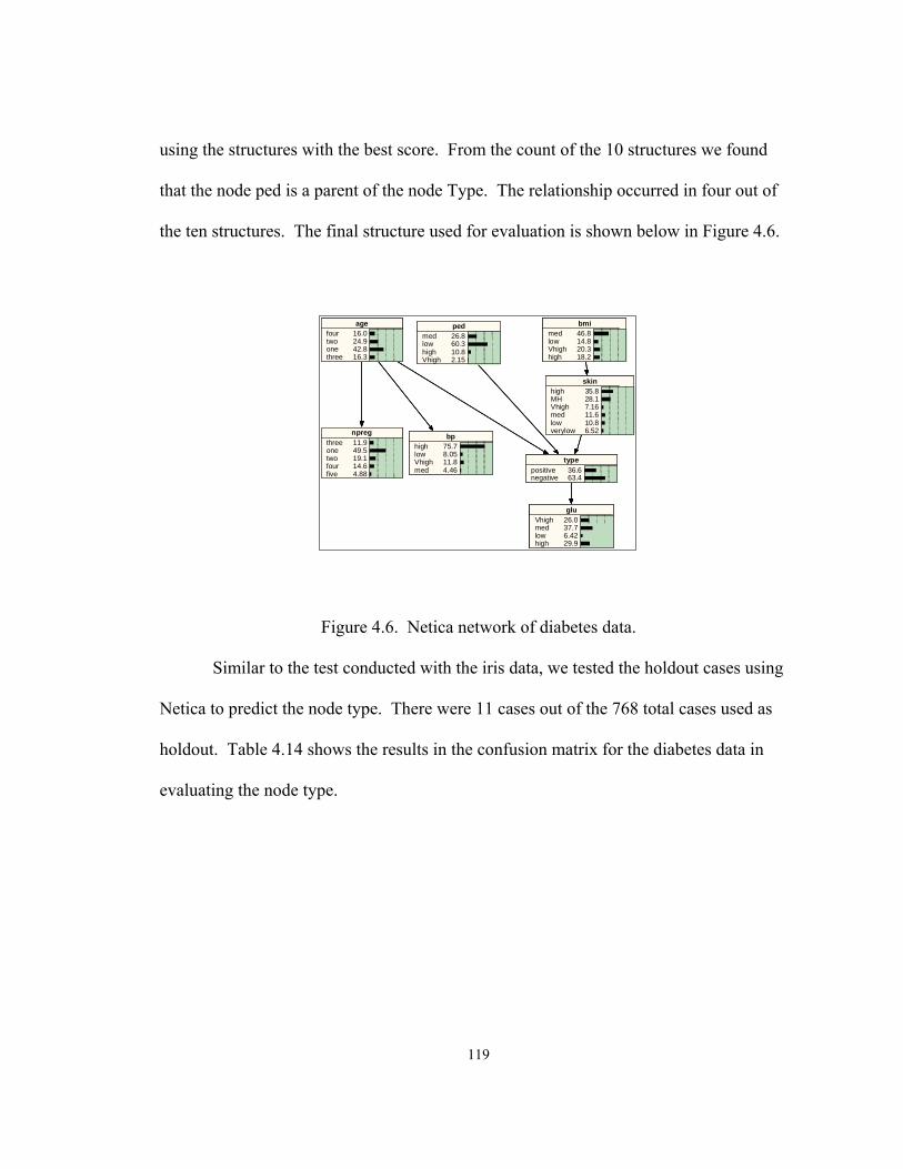
119
using the structures with the best score. From the count of the 10 structures we found
that the node ped is a parent of the node Type. The relationship occurred in four out of
the ten structures. The final structure used for evaluation is shown below in Figure 4.6.
Figure 4.6. Netica network of diabetes data.
Similar to the test conducted with the iris data, we tested the holdout cases using
Netica to predict the node type. There were 11 cases out of the 768 total cases used as
holdout. Table 4.14 shows the results in the confusion matrix for the diabetes data in
evaluating the node type.
npregthreeonetwofourfive
11.949.519.114.64.88
agefourtwoonethree
16.024.942.816.3
bphighlowVhighmed
75.78.0511.84.46
bmimedlowVhighhigh
46.814.820.318.2
typepositivenegative
36.663.4
gluVhighmedlowhigh
26.037.76.4229.9
skinhighMHVhighmedlowverylow
35.828.17.1611.610.86.52
pedmedlowhighVhigh
26.860.310.82.15

120
Table 4.14. Confusion matrix for the node Type for Diabetes data (1).
Unlike the iris data results, the diabetes had a very small error associated with
predicting the node type, only 9.09%. This means that for 9% of the cases in which a
value for the node type was provided the network predicted the wrong value. The low
error rate could be due to more cases for this dataset. The iris dataset had had a very
small dataset with only 150 cases compared to 768 for diabetes. Also, as previously
noted, there was overlap with the different species in which two species could have
similar measurements. It appears that the categories for detecting diabetes are more
distinguishable and therefore causes less error.
In an additional test of the diabetes data, we evaluated the predictive accuracy of
our model for predicting positive or negative test to determine if a person had diabetes.
The resulting confusion matrix (Table 4.15) shows that the error rate overall increased to
17.45%. Out of the 74 known cases of the diabetes being positive, the model only
For type:--------Confusion:
...Predicted..positive negative Actual------ ------ ------
4 1 positive0 6 negative
Error rate = 9.09%
Scoring Rule Results:Logarithmic loss = 0.3259
Quadratic loss = 0.1844Spherical payoff = 0.9028

121
predicted 71% accurately in all cases. But out of the 217 known cases the model
correctly predicted 88% of the cases for negative.
Table 4.15. Confusion matrix for the node Type for Diabetes data (2).
To summarize the predictive data graphically we used a Receiver Operating
Characteristic (ROC) curve. The ROC curve is created by plotting the true positive rate
against false positive rates or sensitivity (1-specificity). The ROC curve goes from
bottom left to upper right. Perfect classifier would follow left and upper axes. Real
classifiers lie in between these two cases (i.e. upper left triangle of the graph). Figure 4.7
of a Receiver Operating Characteristic (ROC) shows the results of testing the
classification accuracy of the model for diabetes with 768 cases.
For type:--------Confusion
...Predicted..positive negativeActual------ ------ ------
74 30positive26 191negative
Error rate = 17.45%
Scoring Rule Results= 0.4059= 0.2587= 0.8568
Logarithmic lQuadratic Spherical
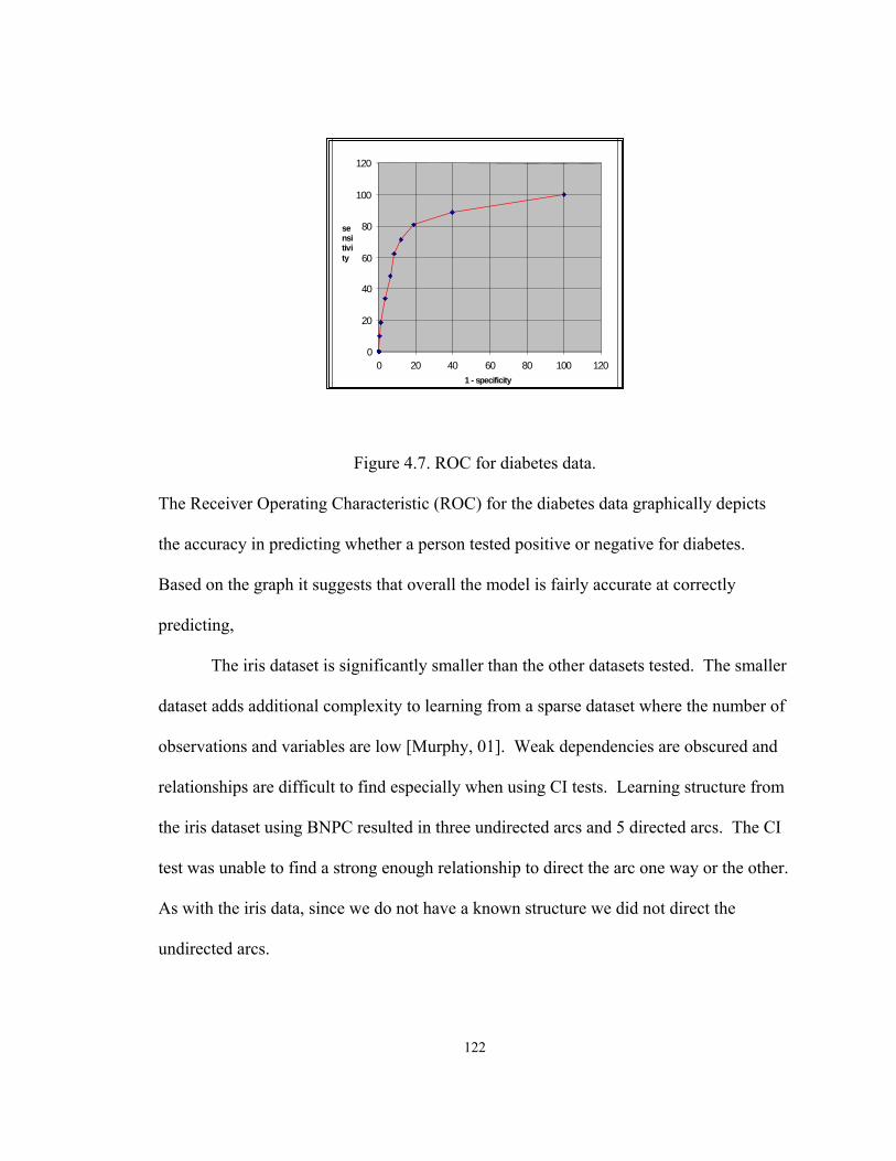
122
Figure 4.7. ROC for diabetes data.
The Receiver Operating Characteristic (ROC) for the diabetes data graphically depicts
the accuracy in predicting whether a person tested positive or negative for diabetes.
Based on the graph it suggests that overall the model is fairly accurate at correctly
predicting,
The iris dataset is significantly smaller than the other datasets tested. The smaller
dataset adds additional complexity to learning from a sparse dataset where the number of
observations and variables are low [Murphy, 01]. Weak dependencies are obscured and
relationships are difficult to find especially when using CI tests. Learning structure from
the iris dataset using BNPC resulted in three undirected arcs and 5 directed arcs. The CI
test was unable to find a strong enough relationship to direct the arc one way or the other.
As with the iris data, since we do not have a known structure we did not direct the
undirected arcs.
0
20
40
60
80
100
120
0 20 40 60 80 100 1201 - specificity
sensitivity

123
4.2.2 Hypothesis II: Continuous variables with observations missing at random (MAR)
can be discretized successfully by combining a Monte Carlo method for filling in the
missing data with a stochastic search over discretization policies.
The same process of interleaving discretization and structure learning was
conducted on the dataset, Asia, with data missing. We mimicked a previous study, which
noted that for most datasets with missing values the percentage of missing values is
relatively low, less than 10 to 15% [Friedman, 97]. In the study conducted by Friedman
for learning belief networks with missing data, he randomly removed values from the
training sets with a varying percentage of missing data. Similarly, we chose to randomly
remove 1%, 5% and 10% of the data from the Asia dataset.
The PopMCMC program, as previously discussed can generate missing values.
The program also generates multiple structures based on user input. For each dataset
with a percentage of missing data we had PopMCMC generate a total of 10 structures for
each of the 10 cycles with one structure having the best BD score. From the 10 best
structures we compared the BD score and counted the number of correct arcs. Table 4.16
shows the results based on the best structure and the percent of missing data.
Table 4.16. PopMCMC results for percentage of missing data for Asia network.
PopMCMC % Missing Data # True Arcs # Error Arcs # Correct
Arcs # Missing
Arcs BD Score
1% 8 7 7 0 -1.3457 5% 8 9 6 0 -1.3283 10% 8 6 7 0 -1.3228

124
The one and five percent missing data were run for 10 cycles of discretization and
structure learning. The structure learning program was set at 100 iterations. However,
for the 10% missing data we set the PopMCMC iterations to 1000 since we deduced that
the performance would degrade with an increase in missing data based on previous
studies [Friedman, 97]. We were able to mitigate some of the missing data effects with
increased numbers of iterations. If we assume this is a modest percentage of missing data
we should expect the degradation in the scores to be modest or non-existent [Chickering
and Heckerman, 96]. In comparing the scores we note that there is minimal degradation
as the percentage of missing data increases from 1 to 5 and finally to 10 percent. We also
noted that the missing data BD scores were similar to the BD score without missing data
and the number of correct arcs increased. We were unable to compare the PopMCMC
process to BNPC because BNPC cannot generate missing data values.
4.2.3 Hypothesis III: The performance of a discretization algorithm shows a measurable
degradation as the amount of missing data increases.
In order to evaluate our process with missing data to another documented process
we replicated a previously published experiment using the dataset Alarm [Friedman,
1997]. This artificial network has known structure with 37 discrete nodes. We evaluated
our process with 10 and 20% missing data to the published results for Alarm. These
percentages were chosen since there was negligible degradation in the scores until there
was 10% missing data. The published study found the greatest change in score was an
increase in missing date from 10 to 20%. Similar to the previous experiment we
randomly removed values using 500 samples. The results are shown in the figure below.

125
Alarm data
-25
-20
-15
-10
-5
00 10% 20%
Percent Missing Values
Sco
re PopMCMCFreidman
Figure 4.8. Comparison of methods with percentage of missing values.
In comparing the process used in the published study to ours it is important to
note the differences. The method for learning used in the study, [Freidman, 97] used a
variant of the EM algorithm to score the learned structures from missing data. Their
process does not find missing values; rather their process evaluates how well the learned
structure models the target distribution. Their process starts with an arbitrary initial
structure and evaluates the structure based on a score. The structure with the highest
score is chosen. As Figure 4.8 demonstrates the degradation in performance is not
significant with the increase in missing data for either process. The authors of the study
suspected that the slight improvement for the 10% missing values was due to the
randomness of their process. They concluded that the randomness allowed the search to
escape some of the local maxima found when there are no missing values [Freidman, 97].
The EM process does not interleave learning structure with discretization and the dataset

126
was discrete. Based on the results, we believe our process shows promise in learning
unknown structure with continuous variables and missing data.
4.2.4 Hypothesis IV: When structure is unknown, and/or there is a relatively large
amount of missing data, Arc counts over multiple structures and discretization policies
will result in more accurate inferences than using a single ‘best’ model.
Our last evaluation was to evaluate how well conducting an arc count over
multiple structures would perform when there is in missing data and one model does not
dominate the other models. We once again used the Asia dataset with 10% missing. We
evaluated the impact of increasing the number of iterations from 100 to 1000 with 10
cycles of interleaving learning and discretization. The structure converged more quickly
to the correct structure after 3 cycles with only one error. However, the structure with the
least number of errors did not have the lowest score. The structure with the lowest BD
score had three errors. Each cycle produced a population of 10 structures with one
structure resulting as the best with the lowest BD score. The table below shows the
results of each cycle for 10 cycles total with the number of incorrect arcs, number of
correct arcs and the BD score for the best structure.

127
Table 4.17. PopMCMC results for 10 cycles 1000 iterations for Asia dataset.
Cycle # Error Arcs # Correct Arcs BD Score 1st Cycle 1 (best) 10 -1.1927 2nd Cycle 9 7 -1.1934 3rd Cycle 8 7 -1.1933 4th Cycle 5 9 -1.1919 5th Cycle 6 8 -1.1922 6th Cycle 3 9 -1.1913 7th Cycle 5 9 -1.1920 8th Cycle 3 9 -1.1912 (best score) 9th Cycle 6 6 -1.1924 10th Cycle 5 8 -1.1929
The results from the 1000 iterations show that the best BD score does not equate
to the fewest errors. The results in the 8th cycle had the best score, but not the fewest
errors. The structure from the first cycle had the fewest error but the 7th best score.
Overall, only one structure, the best in the first cycle, found the correct relationship
between the nodes Visit to Asia and TB. The lack of an arc between the two nodes due to
the weak relationship was expected as previously discussed. Additionally, all 10 best
structures found the nodes Smoking and Visit to Asia as parent nodes. We can conclude
that when there is no missing data, for a noncomplex network our process can find an
accurate structure to represent the dataset using discretization with structure learning.
We can also conclude that more than one structure could represent the dataset if we used
only the BD score. As observed from the BD scores shown in Table 4.17, the difference
in the scores between the runs is not very large.

128
Table 4.18. Arc count between nodes for Asia dataset.
Parent Node Child Node 1 2 3 4 5 6 7 8 TB (1) 0 0 0 0 1 0 0 0
Xray (2) 0 0 9 0 10 0 0 3 Abnormality (3) 10 0 0 0 0 0 0 7
Dyspnea (4) 0 0 9 0 7 0 10 2 Visit to Asia (5) 0 0 0 0 0 0 0 0
Smoking (6) 0 0 0 0 0 0 0 0 Bronchitis (7) 2 0 0 0 0 10 0 0
Lung Cancer (8) 5 0 4 0 0 6 0 0
Due to the close BD scores we examined the arc relationships between nodes. In
Table 4.18 the names of the nodes are listed in the far left column and represent the child
nodes or descendent. The top row represents the parent nodes. There is a direct
dependency between two nodes if there is an arc from the parent node to the child node.
The table above depicts the number of times an arc exists between two nodes in the 10
best structures learned. The arc count indicates that out of the eight correct arcs in the
known network, our process found five of the correct arcs 10 out of the 10 cycles to
include the two parent nodes, Smoking and Visit to Asia. The process of interleaving
discretization with learning structure resulted in the correct relationships between
Dyspnea, XRay and Abnormality nodes nine out of 10 times. The correct relationship is
shown in Table 4.19.

129
Table 4.19. Correct Asia dependencies.
Child node Parent node TB Visit to Asia
XRay Abnormality Abnormality TB Lung Cancer
Dyspnea Abnormality Bronchitis Visit to Asia
Smoking Bronchitis Smoking
Lung Cancer Smoking
The discretization with structure learning had difficulty finding the correct
relationship between TB and Visit to Asia as previously discussed. The process also was
evenly divided over the node relationships for Lung Cancer. The correct parent for Lung
Cancer was Smoking but our process found Abnormality as the parent node four out of
10 times. As with TB, the process could not find clearly discern the relationships for
Lung Cancer among the three nodes because the dependency between the nodes was too
weak.
We compared our results to a similar study conducted by the author of BNPC. In
that study the dataset was discrete and 1000 cases where used in the experiment for the
dataset Asia. In the experiment for Asia the author had similar results as we reported in
Table 4.10b. The original study was also unable to find a dependency between the two
nodes Visit to Asia and Tuberculosis due to the weak relationship in the dataset and the
small number of cases with “true” values for visit to Asia and/or Tuberculosis. It was
also unable to find the correct edge orientation between Smoking and Lung Cancer as

130
well as between Smoking and Bronchitis. The author noted that this was due to the
limitation of their method [Cheng, et al, 99].
The greater number of iterations allowed PopMCMC to converge to a better
structure with fewer errors. We also observed that as the number of iterations increased
from 100 to 1000 that the CPU time increases by nearly 10 times. This is a disadvantage
with MCMC in that the number of iterations improves the convergence but also increases
the amount of time necessary to reach a stationary distribution. If accuracy in terms of
learned structure, were more important then CPU time our process would be preferred.
4.3 BRAC evaluation
A key step in validating our process was to demonstrate an application to a
complex, real world problem. We applied the interleaving of discretization and structure
learning to the Army’s Base Realignment and Closure (BRAC) historical data from 1988
to 1995. As discussed in the last chapter, the data set is from an approved list of
installations selected for closure or realignment.
The BRAC data set initially consisted of 95 installations and facilities with 38
variables. In this analysis we reduced the number of installations to 41. The initial
dataset included 54 family housing (FH) locations that were eliminated from our dataset
and not used in this study. We eliminated family housing because it is a subset of an
installation and does not represent the true complexities associated with an installation.
The remaining 41 installations were used in three different experiments. The first
experiment included 12 installations that were selected for closure or realignment prior to
BRAC. These installations had negative closure and disposition times. This was due to

131
the method used to calculate closure/disposition times as the difference between the
BRAC round date and the closure/disposition date. Therefore, in one experiment we
retained those 12 installations. In the second experiment we removed these 12
installations reducing the dataset to a total of 29 installations. For a third experiment we
collapsed or eliminated nodes with more than four states in order to reduce the
complexity of the network.
The dataset we used was from an on going BRAC study being conducted by the
United States Military Academy (USMA) student capstone groups [Parnell et al, 2005].
The study, sponsored by the Assistant Secretary of the Army for Infrastructure Analysis
had requested USMA validate their work, a non-Bayesian technique with our model.
Therefore, we used their 29 installations to include the four selected holdout installations.
The four installations were selected randomly from the 29. The holdout installations
were DPSC Philadelphia, Fitzsimmons Army Material Command (AMC), Kelly Support
Center, and Lexington-Bluegrass. Table 4.20 shows the list of the 41 installations used in
both experiments and their respective state. The asterisk next to an installation indicates
it had a negative closure time.

132
Table 4.20. Installations for BRAC study
COMPLETED INSTALLATIONS State
1 Adelphi Woodbridge Res Fac VA*2 Alabama Ammunition Plant AL3 Bayonne Military Ocean Terminal NJ
*4 Big Coppett Key FL*5 Branch USDB, Lompoc CA6 Cameron Station VA
*7 Cape St. George FL8 Coosa River Annex AL9 Detroit Tank Plant MI
10 DMA Herndon VA11 DPSC Philadelphia PA12 East Fort Baker CA13 Fitzsimons AMC CO14 Ft Benjamin Harrison IN15 Ft Chaffee AR16 Ft Des Moines IA17 Ft Devens MA
*18 Ft Dix NJ19 Ft Douglas UT20 Ft Holabird MD21 Ft Indiantown Gap PA
*22 Ft Meade MD23 Ft Missoula MT24 Ft Sheridan IL
*25 Hingham Cohasset MA26 Indiana AAP IN27 Kapalama HI28 Kelly Support Center PA29 Lexington-Bluegrass Army Depot KY30 New Orleans Mil Ocean Terminal LA31 Nike Kansas City 30 MO32 Oakland Army Base CA33 Pontiac Storage Facility MI34 Presidio of San Francisco CA
*35 Recreation Center #2 Ft Bragg NC36 Red River Army Depot TX
*37 Rio Vista USARC CA*38 Sudbury Training Annex MA39 Tooele Army Depot UT
*40 USARC Gaithersburg MD41 Vint Hill Farms Station VA

133
In our experiments there were 38 variables associated with the BRAC data. The
original data was provided by BRACO as compiled by the Office of Economic
Adjustment and refined by the on going study being conducted by USMA student
capstone groups. Several of the original variables had no data available. If no data was
available for any of the installations the variable was discarded. There were originally 79
variables. We reduced the number of variables to 38 for our experiment. There were a
total of 29 continuous variables with the remainder being discrete or nominal. The data
collected on each installation is defined in Table 4.21 as well as the name for BN nodes.
Detailed information on the data can be found at the Office of Economic Adjustment
(OEA) web site4. Future studies could expand the number of variables as data the
collected by the respective Program Managers for each installation becomes publicly
available. The data used in this study was unclassified and available to the public.
4 Office of Economic Adjustment (OEA) web site, http://www.oea.gov/oeaweb.nsf/LIBbyTitle?readform

134
Table 4.21. BRAC variable and node definitions.
Variable Name Node NameNominal, discrete,
continuous DiscriptionCOMPLETED INSTALLATIONS N/A Nominal Installation Name
State State Nominal 2 letter state initialClosure / Realignment CloseReal Nominal Desginated for Closure or Realignment
EPA Region EPAregion Discrete 1 through 9 EPA regions in USSF Starting Inventory SFStart Continuous Super Fund starting inventory
SF to be Disposed disposeSF Continuous Super Fund left to disposeInstallation Type Instaltype Nominal Using established Army references.
MACOM Owner MACOM Nominal Commands.Number of Endangered Species Endangered Nominal No installation had more than 1 endangered species
Superfund Site? Superfund Nominal ID if Superfund siteBRAC Round/Date BRACrd Discrete 1988, 1991, 1993, 1995 assigned numbers 1 to 4
Years to Close YearstoClose Continuous Number of years to closeYears to Dispose DisposeYr Continuous Number of years to dispose
Selling Cost ($000) SellCost Continuous Selling cost of the propertyMunitions & Explosives of Concern
(MEP) UXO Issues (Acres) MEPUXO Continuous Munitions and Explosives of Concern measured in acreageActual Cost to Disposition ($000) ActCost Continuous Measured in dollars
Estimated Environmental Costs EstEnvCost Continuous Measured in dollarsActual Environmental Costs ($000) ActEnvCost Continuous Measured in dollars
Jobs Lost LostJobs Continuous Jobs lost from start of BRACJobs Created JobsGain Continuous Jobs created for base reuse prcess
BAH for O1 w/out dependants BAH ContinuousBasic Allowance for Housing for an 01 without dependents to serve as proxy for land value
% urban/rual PerUrban Continuous Percent of surroundig area and population considered urbanUnemployment % Unemply Continuous Percent estimate of unemployment
Milcon Milcon Continuous facilitiesBRAC FO BRACFOcat Nominal BRAC Field Office Category name
Total Acreage TotalAcre Continuous Measured in acreageDoD Retained Retain Continuous Acreage retained by DoD
DoD Transferred Trans Continuous Acreage transferred to other military departmentExcessed Excessed Continuous Excessed acres remaining
Fed Transferred FedTrans Continuous Acreage transferred to federal agenciesSurplus Surplus Continuous Surplus to Fed
PBTs PBTs Continuous Public Benefit Transfer measured in acresLIFC LIFC Continuous Lease in Furtherance of Conveyance measured in acres
EDCs EDCs Continuous Economic Development Conveyances measured in acresSp. Leg. SpLeg Continuous Special Legislation
Neg. Sales NegSales Continuous Negotiated Sales of propertyPublic Sales PublicSale Continuous Public Sale of property
Surplus Disposed SurplusDis Continuous Surplus Disposed property in acresDisposed Total TotalDispose Continuous Total Disposed property in acres
In many cases, data for all the measurements was not available for all the
installations. In fact, 32% of the data was missing. Due to some of the uncertainties with
the BRAC data minor modifications were required. Some of the data was missing, as
noted but some data was actually zero for various reasons. The PopMCMC program
treats zeros in the data set as missing. Therefore, in places where the data was truly zero,
as was the case with several installations not having unexploded ordinance, we entered a

135
very small number close to zero. The data set was run five iterations for interleaving
learning structure and discretization. Table 4.22 shows the settings for our experiment.
Table 4.22. Settings for BRAC data run.
Discretization Learning Structure Equal
width bins
Num Nodes
Num Continuous
Internal Iterations
Split Prob
Internal Iterations
Num Parents
Num Structures
BRAC 4 37 29 5 .6 100 3 10
Previous studies conducted on the BRAC data were unable to find strong node
relationships. In a study by USMA Systems Engineering Department, the cadets
conducted a multi variable regression analysis using Minitab® software and were unable
to find any strong relationships. They concluded this was due to the scarceness of
historical data available [Parnell et al, 05].
In the first experiment we conducted there were 29 installations. The results of
our experiment with the BRAC dataset determined parent – child relationships among all
the nodes except for PBTs and LIFC. We ran initial tests on the dataset first using all the
installation minus the housing areas (54) and then running only the 29 minus the four
holdout installations. A BRAC expert provided his qualitative impressions of the BN
created by the learning algorithm. The expert concurred with the initial learned structures
we provided.
The second experiment had the 41 installations. For consistency in our
comparisons we used the same four installations as holdouts. Similarly, as with the first

136
experiment, we ran the discretization and structure learning program for five cycles with
the setting the same as shown in Table 4.22. The results of the experiment found
relationships between all the nodes except for ActCost. Based on our results from the
two experiments we evaluated all structures learned in the combined total of ten cycles of
interleaving structure learning and discretization. This gave us a total of 80 structures to
evaluate for each data set. To evaluate the strength of the relationships between nodes we
conducted an arc count for 80 of the structures. The count was done for the 41
installation dataset (BRAC data 3) and for the 29 installation dataset (BRAC data 5). The
result is shown in Table 4.23 of the counts for both data set runs, 160 structures total.
Table 4.23. Arc counts between nodes for BRAC data runs.
i=row childj=columparent
i/j 1 2 3 4 5 6 7 8 9 10 11 12 13 14 15 16 17 18 19 20 21 22 23 24 25 26 27 28 29 30 31 32 33 34 35 36 37 38State 1 0 3 4 3 5 6 8 10 4 3 6 10 2 6 2 6 3 5 3 1 3 4 5 5 2 2 4 6 2 5 4 5 4 4 2 1 4 3CloseReal 2 4 0 2 3 2 5 1 6 5 5 2 3 3 8 3 4 1 0 6 5 8 5 7 5 5 7 2 2 3 4 0 4 3 6 3 4 4 1EPAregion 3 8 1 0 4 3 4 3 10 3 3 2 2 4 1 4 5 5 2 3 9 3 4 3 6 3 7 3 5 3 6 1 7 5 5 3 4 1 1SFStart 4 3 4 4 0 8 3 5 4 5 5 4 2 4 2 5 2 3 4 4 8 3 1 4 4 3 5 9 7 1 9 2 5 7 5 5 4 4 4disposeSF 5 4 4 10 4 0 3 2 2 3 2 5 0 5 2 3 4 5 4 2 4 1 4 3 4 7 2 4 5 6 6 2 3 4 2 5 5 3 0Instaltype 6 2 6 4 3 9 0 5 4 1 4 7 4 3 3 1 8 4 2 6 3 3 5 4 3 4 4 4 4 3 2 1 8 4 4 4 1 1 1MACOM 7 4 7 6 2 4 7 0 9 4 3 9 3 5 6 1 5 2 5 5 2 2 3 5 5 1 4 4 3 4 7 0 5 1 7 4 2 4 2Endangered 8 2 3 2 4 3 7 3 0 2 2 4 5 4 7 4 5 3 1 5 2 0 7 7 4 8 2 4 5 1 8 2 1 1 7 7 2 2 1Superfund 9 2 2 6 3 5 3 5 1 0 4 4 5 3 3 5 3 6 1 5 7 2 6 6 2 4 1 2 3 2 8 3 4 4 3 4 3 4 7BRACrd 10 5 4 2 5 2 6 10 7 5 0 4 5 3 5 3 5 5 5 3 2 3 6 3 5 2 5 2 8 3 2 9 3 8 2 3 6 7 5YearstoClose 11 3 7 3 3 2 5 4 3 4 6 0 7 2 7 6 4 6 4 3 3 3 6 2 0 8 5 1 4 2 6 2 7 2 5 6 3 5 3DisposeYr 12 3 3 2 5 2 6 4 3 5 1 5 0 7 7 6 0 7 3 3 12 6 4 1 10 5 4 6 4 4 3 3 5 2 2 3 3 2 5SellCost 13 3 4 5 4 1 2 3 4 3 6 4 4 0 3 3 4 3 3 5 6 4 2 4 5 2 3 2 3 3 4 1 1 3 4 6 1 5 4MEPUXO 14 3 0 3 3 3 8 5 3 6 4 6 1 3 0 3 5 6 5 4 5 0 7 2 4 9 4 4 4 1 6 5 9 2 4 5 3 8 4ActCost 15 2 5 7 4 4 5 8 3 4 4 1 3 4 4 0 2 2 5 5 5 5 0 6 3 3 2 2 9 3 4 3 5 1 4 0 5 2 4EstEnvCost 16 5 5 5 2 5 3 5 2 0 4 4 2 2 8 4 0 3 8 5 1 5 3 3 4 3 3 3 7 3 5 3 7 3 4 8 4 3 5ActEnvCost 17 1 0 4 6 3 4 5 6 5 7 5 3 5 4 2 3 0 5 7 5 3 0 4 4 2 2 8 0 3 4 7 2 2 4 4 2 4 5
LostJobs 18 5 4 2 7 4 3 1 5 6 0 6 1 5 6 4 2 3 0 2 9 3 4 7 4 3 5 2 2 3 3 5 2 0 7 4 3 4 1JobsGain 19 2 3 4 5 5 1 5 2 5 4 4 3 4 5 5 3 3 5 0 3 9 4 4 3 4 3 4 6 4 5 4 2 1 4 8 3 4 4BAH 20 3 5 2 6 4 3 9 11 6 7 4 4 3 2 1 3 6 4 4 0 2 2 7 2 3 1 7 6 6 4 3 2 3 5 6 4 7 2PerUrban 21 3 7 4 6 5 4 6 5 6 2 5 6 6 5 5 1 4 5 4 9 0 0 1 3 2 2 7 3 4 5 4 4 7 3 5 3 1 2Unemply 22 5 0 2 5 4 3 8 3 3 3 7 6 5 3 6 6 5 1 4 6 5 0 3 8 4 5 8 5 5 6 5 5 7 5 2 3 1 3Milcon 23 2 3 4 3 5 3 3 5 1 3 4 1 5 6 4 1 6 4 4 2 4 5 0 4 4 2 5 6 2 5 4 3 5 4 6 3 8 5BRACFOcat 24 6 3 3 1 3 3 5 3 2 3 6 4 3 1 3 2 4 2 2 5 4 6 3 0 4 5 1 4 0 3 6 12 9 7 8 4 3 5TotalAcre 25 5 2 4 4 4 0 5 5 0 4 7 6 4 4 5 3 4 5 5 5 1 4 3 5 0 8 5 2 9 4 2 9 3 3 3 1 4 5Retain 26 6 4 7 6 7 3 2 3 4 2 5 7 4 2 5 5 4 2 8 1 2 4 5 2 5 0 8 5 3 2 2 9 2 2 4 2 2 3Trans 27 2 7 4 3 3 5 7 6 2 6 7 5 0 2 2 3 3 2 4 3 2 6 6 4 7 2 0 2 2 5 7 6 2 2 10 9 4 2Excessed 28 3 1 6 1 5 1 2 8 2 4 3 3 7 5 2 12 0 4 2 7 2 3 5 1 8 1 5 0 3 3 4 4 3 3 5 3 3 3FedTrans 29 6 5 6 6 3 4 1 8 1 7 2 5 2 5 3 10 5 1 4 3 3 3 6 10 6 3 4 4 0 4 6 5 4 4 6 4 2 4Surplus 30 1 5 4 3 3 3 6 6 1 3 5 7 1 8 2 2 7 6 1 2 3 3 7 2 4 2 3 9 4 0 6 6 3 6 7 5 8 6PBTs 31 3 6 6 3 10 3 5 6 2 4 3 5 3 3 3 7 6 5 1 4 5 1 3 3 6 0 4 1 2 5 0 3 3 5 6 5 3 6LIFC 32 5 4 4 5 4 8 2 7 5 6 2 2 4 3 2 3 4 1 5 4 7 2 6 5 2 4 5 1 0 4 7 0 8 4 6 5 6 3EDCs 33 4 5 5 3 3 4 9 2 6 4 6 6 6 3 4 5 0 3 5 6 3 8 3 6 2 2 4 4 7 5 2 1 0 5 6 5 4 2SpLeg 34 3 4 6 4 3 2 7 3 4 0 6 4 6 3 4 9 5 2 3 6 4 4 2 1 4 2 4 8 4 6 5 6 0 0 4 3 7 2NegSales 35 2 5 7 3 5 2 6 5 1 8 5 4 6 3 4 5 3 5 2 1 4 4 4 8 4 3 7 3 6 3 8 2 7 7 0 4 4 10PublicSale 36 7 3 2 3 5 3 2 5 4 1 7 4 5 4 7 2 3 3 7 6 5 6 6 3 4 5 1 4 6 3 2 3 3 6 3 0 2 2SurplusDis 37 1 3 6 5 6 5 3 3 5 4 2 4 8 7 5 5 7 7 3 8 9 4 8 5 1 3 3 5 3 5 6 7 5 2 2 2 0 7TotalDispose 38 2 4 7 6 3 3 2 7 3 1 6 4 4 8 8 3 4 4 0 3 4 7 2 3 2 2 4 4 5 6 3 3 4 4 7 3 8 0

137
In the figure above, the rows represent the child node and the columns the parent
node. The number annotated in the cell indicates an arc from the parent to the child node.
The diagonal is zero since a node cannot be a parent to itself. Evaluating Table 4.23 we
noted that all nodes have a causal relationship or at least one arc. The chart is color
coded in order to find relationships. We arbitrarily set a threshold count at greater than
five to find relationships. If we raise the threshold from five to eight and found that 32
out of the 38 nodes meet or exceed the new threshold, meaning that the probability of
having an arc to a particular node increased. We found a count of 12 to be the highest
occurrence in the experiment, of which only three out of the 38 nodes meet that
threshold. The red indicates no relationship or zero count. Also, a node was not allowed
to be its own parent as noted by the zeros on the diagonal in Table 4.23.
The dataset we used to build the primary Bayesian network was from the 29
installations, minus the four holdout installations. We used the best generated structure
based on BD score from our process of interleaving structure learning and discretization.
The nodes were imported into Netica and arcs were added based on the learned structure.
Our best structure did not find relationships for two of the nodes and required us to add
arc. We could have deleted the nodes but based on the total arc count from the 80 runs
we determined there was a relationship between PBTs and disposeSF. There was an arc
count of 10 between the two with disposeSF as the parent and PBTs as the child.
Similarly we found LIFC had a strong relation between MACOM, EDCs and
BRACFOcat. They had a count of eight respectively with MACOM and EDCs as the
parent nodes and LIFC as the child. There was a count of 12 between the nodes LIFC

138
and BRACFOcat with LIFC as the parent node. The low probabilities associated with the
arc count can be explained by the uncertainty associated with the BRAC dataset due to
sparseness.
The two nodes that did not have arcs we used two sources to assist us in
determining where to add arcs. We used the documentation on the BRAC process and
the arc counts learned to assist in determining relationships. In our process two nodes did
not have arcs. We found the arc counts conducted on the structures learned closely
resembled the documented BRAC process and therefore allowed us to justify the adding
of arcs to the nodes with no relations, PBT and LIFC. Both nodes, PBT and LIFC are
part of a process to dispose of excess property. The highest arc counts related to the two
nodes were with nodes that impact land transfer. The BRAC process deems land not
needed by DOD as excess and can be disposed of through various means. The excess
land can be transferred to Local Redevelopment Authorities (LRA) for Public Benefit
(PBT) purpose, which is a subset of the Economic Development Conveyances (EDC)
process. The PBT allows local agencies to acquire the property for public use purposes
such as schools, airports, etc. The EDCs allows the property to be sold at or below fair
market value to revitalize the economy and ease the economic impact caused by the
BRAC process. The LIFC is another form of transferring property prior to PBT under the
EDC process. The lease allows property that cannot be sold due to environmental
requirements to be leases to agencies for economic development.
The relationships learned were imported to Netica and tested using the four
holdout installations. The four installations were DPSC Philadelphia, Fitzsimons AMC,

139
Kelly Support Center, and Lexington-Bluegrass. Evidence we knew was entered for the
BN in Netica. For example, if we desired to predict the years to close an installation on
the BRAC list, we would know the location (state), the type of installation, the MACOM
owner, the BRAC round, the BRAC field office responsible for the installation, whether
the installation is a superfund site or not, the EPA region where the installation is located
and whether the installation was on the closure or realignment list. The affected nodes
and the evidence known for DPSC Philadelphia are shown in Table 4.24 and Figure 4.9.
Table 4.24. Evidence entered on known nodes.
Node Evidence Known Superfund Yes Instaltype DLA EPAregion Three MACOM DLA BRACrd Three BRACFOcat Two State PA CloseReal CLOSE

140
Figure 4.9. Learned BN in Netica for DPSC Philadelphia with entered evidence.
We found that the network provided accurate predictions on the years to close and
years to dispose. In the case of DPSC Philadelphia, the true time for year to close the
installation was 6.03 and 8.27 for years to dispose. Our model predicted with a 72%
probability that the years to close would be in the medium category. Likewise, the model
showed a 40.3% probability the installation would fall in the long category for years to
dispose. All the holdout installations were compared in the same manner as DPSC
Philadelphia. Table 4.25 shows the results of the predicted probabilities of years to close
using the learned BN in Netica for all four holdout installations.
REALIGN 0
CloseReal
LIFCEstEnvCost
InstaltypeYearstoClose
Endangered
TotalDispose
FedTrans
DisposeYr
NegSales
ActCost
MACOM
LostJobs
BRACFOcat
ActEnvCost
BRACrd
disposeSF
SFStart
Milcon
SurplusDis
SellCost
TotalAcre
PublicSale
PBTs
Superfund
Unemply
JobsGain
MEPUXO
PerUrban
Excessed
Surplus
EPAregion
BAH
State
CLOSE 100
med 19.3high 12.5low 42.8Exhigh 25.4
Transmed 25.5Exhigh 30.2low 19.6high 24.7
EDCs FedTrans
low 40.1high 27.9med 18.5Exhigh 13.5
low 93.7high 2.07med 2.79Exhigh 1.40
low 33.1Exhigh 18.9high 21.6med 26.3
low 49.3high 14.2Exhigh 18.6med 18.0
high 35.0Exhigh 25.9low 23.0med 16.1
Exhigh 5.81high 5.74med 38.2low 50.3
Exlg 24.0small 38.3large 20.1med 17.6
Exhigh 24.8low 26.1high 27.7med 21.4
high 23.8low 36.3med 20.0Exhigh 20.0
low 64.8med 12.5Exhigh 11.4high 11.4
low 23.6Exhigh 12.2high 37.8med 26.4
med 72.0long 11.3Exlong 8.43short 8.31
high 26.4Exhigh 23.4low 23.4med 26.8
med 52.1low 15.3high 15.9Exhigh 16.7
low 40.6med 35.4high 7.10Exhigh 17.0
med 22.9small 48.6Exlg 14.3large 14.3
Exhigh 26.6low 31.0high 21.5med 20.9
med 21.9low 60.0Exhigh 10.6high 7.73
IN 0UT 0IL 0MA 0VA 0NJ 0Al 0MI 0CO 0PA 100MT 0LA 0CA 0TX 0HI 0AR 0
Retain
two 100one 0three 0
low 75.6Exhigh 13.5med 11.0-
low 89.8med 5.92Exhigh 4.25
high 22.9Exhigh 56.2low 20.9
No 86.0Yes 14.0
five 0eight 0one 0three 100two 0four 0six 0nine 0
Ind 0Admin 0Labs 0Med 0USAR 0Depot 0DLA 100Tran 0Active 0
med 20.9low 34.8Exhigh 44.2
One 0Four 0Two 0Three 100
med 17.3short 19.0Exlong 23.4long 40.3
AMC 0USARC 0DLA 100FORSCOM 0MTMC 0MDW 0MEDCOM 0INSCOM 0TRADOC 0USARPAC 0
No 100Yes 0
low 82.0med 10.0Exhigh 3.54high 4.41 low 43.5
high 16.4Exhigh 14.5med 25.6
large 18.3small 41.5med 24.6Exhigh 15.6
med 41.9Exhigh 21.7high 36.4
DPSC Philadelphia (bracdata5.txt)

141
Table 4.25. Cutpoints learned and prediction probabilities for BRAC data.
Predicted probabilities for Years to Close Installation Actual 0 ≤ short
<3.19 3.19 ≤ med <6.21
6.21 ≤ long <7.21
Exlong ≥7.21
DPSC Phil 6.03 8.31 72.0 11.3 8.43 Fitzsimons 3.97 8.36 72.1 11.2 8.41 Kelly 4.87 5.96 78.3 9.8 5.94 Lexington 3.21 9.71 69.8 11.7 8.84 Predicted probabilities for Years to Dispose Installation Actual 0 ≤ short
<4.14 4.14 ≤ med <7.24
7.24≤ long <10.68
Exlong≥10.68
DPSC Phil 8.27 19.0 17.3 40.3 23.4 Fitzsimons 7.97 19.6 17.8 44.1 18.5 Kelly 7.90 12.2 27.7 44.5 15.5 Lexington 7.21 17.0 32.4 28.8 21.8
The result of the experiment provides an accurate predictor based on known
evidence from the BRAC real data on time to close. The only installation that did not
clearly fall into one time category was Lexington-Bluegrass Army Depot. The model
predicted the correct category of medium but there was only a small difference between
medium and the long category, 32.4 and 28.8% respectively. The actual time to dispose
of the property based on historical BRAC data was7.21 years, which is near the cutpoint
for the two categories. If we entered evidence on the node for total acreage of the
installation (TotalAcre) as low, the probabilities change. The new probabilities only
slightly increased for the node DisposeYr. The new probability for the category ‘med’
changed from 32.4 to to 33%, and increased the probability for the category ‘long’ from
28.8 to 29.2%. However, in conducting sensitivity analysis on the variable years to

142
dispose (DisposeYr) for the Lexington-Bluegrass installation, we found it is most
sensitive to the variables actual cost and lost jobs.
Table 4.26. Sensitivity of years to dispose to other variables.
Node Mutual information Quadratic score ActCost 0.04025 0.0044453 LostJobs 0.01460 0.0020295
We found the node DisposeYr is not highly sensitive to any other node in the
network as noted by the quadratic score. A quadratic score close to zero would mean
there is little effect. The nodes listed in Table 4.26 above had the only real measurable
effect on DisposeYr. By entering evidence for the two nodes we could make a
measurable impact on the probability to dispose for DPSC Philadelphia. If we change the
evidence entered on the node ActCost to medium and on the node LostJobs to low, the
probability for long decreases and the other three categories increase. The probability for
a long dispose time would result in a significant decease from 40.3 to 22.4% for the
installation. The entering of evidence causes an increase of uncertainty in the disposition
time. Further evaluation would be needed to increase the probability in one time
category or the other. Similarly for YearstoClose there were no nodes that had
significant effect on the predicted duration for closing.

143
Table 4.27. Sensitivity of years to close to other variables.
Node Mutual information Quadratic score SFStart 0.04119 0.0058399 EstEnvCost 0.03501 0.0053075
As the table above shows, the node YearstoClose is only sensitive to two
variables, both have a low quadratic score. If we place evidence on the node for the
superfund start (SFStart) to medium it increased the predictive probability for the node
YearstoClose. The entering of evidence on SFStart changes the predictive probability for
the category medium from 69.8 to 76.9%.
The BRAC 2005 Strategic Plan developed by the TABS office set the goal of
closing or realigning 60% of the installations within three years or less and disposing of
60% of the installations under six years. Our current evaluation of the BRAC data found
that all four holdout installations fell within the desired category for closure, but only one
of the four did for disposal. The cutpoints found by our process does not allow us to set
the bins to specifically capture the range of three years or less. The cutpoints, as
previously discussed were found through a search and score process. The cutpoints with
the highest score were retained. However, we can use the cutpoints with the BN to
evaluate courses of action that could reduce the years to close or dispose of an
installation.
The BRAC dataset with 29 installations was also evaluated using the BNPC
software. The program found undirected relationships for all 38 nodes and only one

144
parent node, state. Since there was only one parent node, the undirected nodes had to be
manually directed. The edited network was exported to Netica to evaluate the prediction
capability for the years to close and years to dispose.
Table 4.28. Cutpoints and prediction probabilities for BRAC data with holdouts. Predicted probabilities for Years to Close Installation Actual 0 ≤ short
<3.19 3.19 ≤ med <6.21
6.21 ≤ long <7.21
Exlong ≥7.21
DPSC Phil 6.03 15.6 15.6 53.1 15.6 Fitzsimons 3.97 20.8 20.8 37.5 20.8 Kelly 4.87 15.6 15.6 53.1 15.6 Lexington 3.21 21.5 20.6 37.6 20.3 Predicted probabilities for Years to Dispose Installation Actual 0 ≤ short
<4.14 4.14 ≤ med <7.24
7.24≤ long <10.68
Exlong≥10.68
DPSC Phil 8.27 15.6 40.6 28.1 15.6 Fitzsimons 7.97 20.8 37.5 20.8 20.8 Kelly 7.90 15.6 40.6 28.1 15.6 Lexington 7.21 25.1 27.6 27.2 20.1
The predictive capability of the BNPC network did not perform as well as the
network learned by our process, PopMCMC. After entering known evidence for each
installation the probabilities to predict years to close and dispose were recorded as shown
in Table 4.28. The probabilities for the node years to close predicted the time category
long for all three installations. The numbers of years to close DPSC Philadelphia is close
to the cutpoint but the probabilities for medium and long are not close to the true number.

145
The model predicts a long time period with a 53.1% probability verses a medium period
of 15.6%.
The prediction for years to dispose installations also performed poorly. Three of
the predictions show a high probability of taking a long period of time to dispose when
they actually were in the medium time range. One installation, Lexington-Bluegrass, has
an actual disposal time of 7.21 years, which is close to the found cutpoint of 7.21 years.
The network predicted similar probabilities for the medium and long time category for
Lexington-Bluegrass. The probabilities were 27.6 and 27.2 for the respective categories.
A similar probability was associated with the small time category, which means there is
uncertainty in accurately predicting the time to dispose based on the available evidence.
The BNPC, using the same dataset was unable to find any strong relationships
between nodes. We expected this result since a previous study that used multivariable
regression analysis [Parnell et al, 05] was also unable to find strong relationships.
Additionally, the dataset is small and sparse which places limitations on the CI test in
BNPC to find any strong relationships.
To handle uncertainty when the structure is unknown and the dataset is sparse we
had hypothesized that using an arc count could result in more accurate inferences than a
single ‘best’ model. The approach we took to evaluate the multiple structures was to take
the arc counts of all the structures and use the highest counts to build the model. The
structures used for the arc count process were from the BRAC dataset with the 29
installations in which four were holdouts. We ran our process for 10 cycles, creating 10
structures each cycle. The first cycle was used to initialize our process since it uses equal

146
width binning to find an initial structure. A total of 10 cycles were used for the structure
based on highest arc count. The threshold was set at greater than eight for the arc count
to be used in the parent – child relationship between nodes. The nodes meeting or
exceeding the threshold were used for the relationship table. The bold child node
indicates those nodes are a parent node. The shaded cell indicates the node with the
highest arc count. Table 4.29 shows the relationships between nodes.
Table 4.29. Node relationships based on arc counts for BRAC data.
based on arc countbracdata5.txtChild i/j Parent Parent Parent ParentState 1 Endangered DisposeYrCloseReal 2 MEPUXO ActEnvCostEPAregion 3 Endangered BAHSFStart 4 Trans SurplusdisposeSF 5 EPAregionInstaltype 6 disposeSFMACOM 7 Endangered YearstoCloseEndangered 8Superfund 9 RetainBRACrd 10 MACOM PBTsYearstoClose 11DisposeYr 12 BAH BRACFOcatSellCost 13MEPUXO 14 TotalAcre LIFCActCost 15 ExcessedEstEnvCost 16ActEnvCost 17 MilconLostJobs 18 BAHJobsGain 19 PerUrbanBAH 20 MACOM EndangeredPerUrban 21 BAHUnemply 22 EPAregion BAH MilconMilcon 23BRACFOcat 24 LIFC EDCsTotalAcre 25 Surplus LIFCRetain 26 LIFCTrans 27 NegSales PublicSaleExcessed 28 EstEnvCostFedTrans 29 EstEnvCost BRACFOcatSurplus 30 ExcessedPBTs 31 disposeSFLIFC 32 Instaltype EDCsEDCs 33 MACOMSpLeg 34 EstEnvCostNegSales 35 TotalDisposePublicSale 36 State YearstoClose ActCost JobGainSurplusDis 37 PerUrban SellCostTotalDispose 38 MEPUXO ActCost EDCs

147
The relationships shown in Table 4.28 were used to develop a network in Netica.
The case file for the 25 installations was incorporated into the model to learn the
probabilities. We used the holdout installations to test the model’s ability to accurately
predict the correct year category for both closure and disposal. The known information
for the installations was used as the evidence placed on the node. Table 4.30 shows the
holdout installations and the known evidence entered on the nodes.
Table 4.30. BRAC holdout installations for prediction capability.
Using the holdout installations we evaluated how well our model would
accurately predict the years to close (YeartoClose) and years to dispose (DisposeYr).
Table 4.30 shows the prediction probabilities of the holdout installations in bold.
Installation State CloseReal EPAregion Instaltype MACOM Superfun
d BRACrd BRACFOcat
DPSC Philadelphia PA close Three DLA DLA No Three twoFitzsimons AMC CO close Eight Med MEDCOM No Four oneKelly Support Center PA realign Three Admin FORSCOMNo Four oneLexington-Bluegrass Army Depot KY close Four Depot AMC No One two

148
Table 4.31. Holdout prediction probabilities by category for BRAC.
Predicted probabilities for Years to Close Installation Actual 0 ≤ short
<3.19 3.19 ≤ med <6.21
6.21 ≤ long <7.21
Exlong ≥7.21
DPSC Phil 6.03 7.03 79.1 7.71 6.2 Fitzsimons 3.97 10.2 68.8 11.8 9.3 Kelly 4.87 3.87 75.2 11.6 9.38 Lexington 3.87 9.93 76.8 4.47 8.77 Predicted probabilities for Years to Dispose Installation Actual 0 ≤ short
<4.14 4.14 ≤ med <7.24
7.24≤ long <10.68
Exlong≥10.68
DPSC Phil 8.27 5.69 29.3 54.7 10.4 Fitzsimons 7.97 18.0 18.2 56.2 7.59 Kelly 7.90 9.75 22.9 55.8 11.6 Lexington 7.21 8.78 44.7 24.6 21.9
We found from our tests on the BRAC data that the model created from the arc
counts provided accurate inference to our queries on the number of years to close and
dispose of installations. In evaluating the structure created using our process, no single
model appeared to be overwhelmingly more probable than others. This was evident by
the BD scores that were not statistically different. We have to be careful not to use these
results to find meaning in the data when there is a large set of possible hypotheses and no
one model significantly out scored other models. The adding of arcs to create
relationships based on arc count for a sparse dataset can cause overfitting. To reduce the
dangers of overfitting we used the four holdout cases to test the prediction performance
and evaluated the predictive capability of our model using the confusion matrix built into
Netica. The confusion matrix confirms our assumptions of our model’s predictive

149
capability when we used the four holdout installations to test our network for the nodes of
interest as shown in Table 4.32
Table 4.32. Confusion matrix results for BRAC network.
The confusion matrix shown above, confirms that for the four holdout cases our
model accurately predicted the correct time category. However, for the node DisposeYr
the model predicted the wrong category for one of the four cases. This prediction error
was the Lexington-Bluegrass installation. We noted previously that the actual time to
dispose was very close to the cutpoint. Also, since there are only four cases used in the
testing of cases, any small error results in a large error rate score. We obtained similar
results using 1000 simulated cases of the BRAC dataset. In that test the error rate for
predicting years to close (YearstoClose) was 32.7% and for years to dispose (DisposeYr)
it was 74.45%.
In the final experiment we collapsed nodes with states greater than four. We
collapsed the number of states because there was insufficient number of occurrences in
For YearstoClose: For DisposeYr:---------------- -------------Confusion: Confusion:
...........Predicted.......... ...........Predicted..........med long Exlong short Actual med short Exlong long Actual------ ------ ------ ------ ------ ------ ------ ------ ------ ------
4 0 0 0 med 0 0 0 0 med0 0 0 0 long 0 0 0 0 short0 0 0 0 Exlong 0 0 0 0 Exlong0 0 0 0 short 1 0 0 3 long
Error rate = 0% Error rate = 25%
Scoring Rule Results: Scoring Rule Results:Logarithmic loss = 0.1811 Logarithmic loss = 0.7591
Quadratic loss = 0.03993 Quadratic loss = 0.3993Spherical payoff = 0.9919 Spherical payoff = 0.7766

150
the data for each of the states to provide any meaningful relationships. The nodes that
were collapsed were the EPA region node (EPAregion) and type of installation
(Instaltype). The EPA regions were combined into three categories based on location.
The new categories for regions were: East, with regions 1-4, Mid, with regions 5-8, and
West, with regions 9 and 10 (California, Hawaii and Alaska). This ensured there were
more than three installations in any one region.
Originally there were 10 MACOMs and 10 types of installations for each node.
The installation type was collapsed down to three categories: Administration, Depot and
Major training activity. The administration category accounted for the installations with
labs, RDT&E, medical facilities and DLA. The Depot category included the industrial
and transportation facilities. The last category encompassed the major training facilities
for both active and reserve as well as housing. The MACOM node for type of command
was combined with installation type (Instaltype) since each MACOM was primarily
associated with a particular type of installation, Table 4.33 depicts the associations. The
node representing the state the installation was located in was deleted due to limited
occurrences for any one state, less than three on average. The collapsing and reduction of
nodes reduced the total from 38 to 36.

151
Table 4.33. MACOM association with installation type.
MACOM Installation Type
INSCOM Depot USARC Admin
AMC Admin FORSCOM Depot
MTMC Training USARPAC Training
MDW Depot TRADOC Admin
DLA Admin MEDCOM Training
The collapsed dataset was run in the same manner as the previous two
experiments. The dataset was run for 10 iterations for interleaving learning structure and
discretization. The settings were the same as shown in Table 4.22. In this experiment we
ran both the 25 and 37 installations with the same four installations as holdouts. In
evaluating the 10 best structures generated, based on their BD score, we found the
structure with the best score to be -1.5867 with 29 installations and -1.0463 for the 37
installations. The best score achieved in the first experiment with 38 nodes and 29
installations was a BD score of -1.8899. Similarly the score for 37 installations with 38
nodes was -1.1357. The reduction in nodes improved the score for both datasets. One
commonality between the two experiments with 37 installations is that the best structures
both did not find any relationships to the node ActCost.

152
We used the dataset from the 37 installations with the reduced nodes to build the
primary Bayesian network, minus the four holdout installations. We used the 10 best
structures generated, based on BD score from our process of interleaving structure
learning and discretization to create the structure in Netica. The nodes were imported
into Netica and arcs were added based on the learned structure. For nodes without arcs
we used the arc count process from the 100 structures to determine the more probable
relationship. There was an arc count of 10 respectively with nodes LIFC and SurplusDis,
with ActCost as the child node. There was also a count of 10 with SFStart, with ActCost
as the parent node. As previously noted, the low probabilities associated with the arc
count can be explained by the uncertainty associated with the BRAC data set due to
sparseness.
In this last experiment with the collapsed nodes we tested 37 installations with
and without evidence entered to evaluate how well the network could predict, specifically
the years to close (YearstoClose) and years to dispose (DisposeYr). The Table below
shows the nodes in which evidence was known for each of the holdout cases.
Table 4.34. Evidence entered on node.
Evidence Known Node Lexington Kelly Fitzsimons DPSC Phil
Superfund No No No No Instaltype Depot Admin Admin Admin EPAregion east east mid east BRACrd One Four Four Three BRACFOcat Two One One Two CloseReal Close Realign Close Close

153
The Table below shows the results for predicting with evidence entered on the
nodes shown in Table 4.34 for each of the holdout installations. The dataset used has the
37 installations with the holdout installations removed.
Table 4.35. Predictions with evidence for 37 installations.
Predicted probabilities for Years to Close Installation Actual 0 ≤ short
<2.25 2.25 ≤ med <3.97
3.97 ≤ long <6.21
Exlong ≥6.21
DPSC Phil 6.03 3.89 12.5 75.6 8.01 Fitzsimons 3.97 3.83 12.3 75.9 7.92 Kelly 4.87 3.89 12.5 75.6 8.01 Lexington 3.87 12.7 13.5 47.8 26.0 Predicted probabilities for Years to Dispose Installation Actual 0 ≤ short
<6.59 6.59 ≤ med <7.97
7.97≤ long <9.98
Exlong≥9.98
DPSC Phil 8.27 24.6 13.2 22.0 40.1 Fitzsimons 7.97 24.6 13.2 22.0 40.1 Kelly 7.90 24.6 13.2 22.0 40.1 Lexington 7.21 24.6 13.2 22.0 40.1
The network correctly predicted the years to close for all the installations except
for the Lexington Bluegrass installations, similar to the first experiment. The model did
not do as well in predicting the years to dispose for the four holdout installations. We
attribute this to the sparseness of the dataset. It incorrectly predicted for all four
installations. As Table 4.35 shows the prediction probabilities for years to dispose did
not change for any of the holdout installations. In testing for sensitivity, the node
‘DisposeYr’ was only sensitive to the node ‘LostJobs’. There appears to be underlying
interactions between the collapsed nodes that at this time, we are unable to detect.

154
We also tested accuracy to predict closing and disposing time using the smaller
dataset with 25 installations. As expected, the accuracy prediction decreased for years to
close, correctly predicting only two of the four installations (Lexington and DPSC
Philadelphia). The years to dispose inaccurately predicted all four holdouts as ranging
between 3.22 and 5.3 years as shown in Table 4.36.
Table 4.36. Predictions with evidence for 25 installations.
Predicted probabilities for Years to Close Installation Actual 0 ≤ short
<4.23 4.23≤ med <6.38
long ≥6.38
DPSC Phil 6.03 31.3 46.0 22.8 Fitzsimons 3.97 53.9 29.8 16.3 Kelly 4.87 54.2 30.2 15.6 Lexington 3.87 24.1 51.9 24.0 Predicted probabilities for Years to Dispose Installation Actual 0 ≤ short
<3.22 3.22≤ med <5.30
long≥5.30
DPSC Phil 8.27 20.7 47.5 31.8 Fitzsimons 7.97 19.9 48.7 31.4 Kelly 7.90 21.7 47.5 30.8 Lexington 7.21 19.9 49.5 30.6
We had suspected that reducing the number of nodes and states would reduce the
complexity of the model and thus provide better prediction results. This was not the case
when we evaluated our models using the four holdout cases with evidence. In testing our
two structures without evidence we found the models accurately predicted the years to
close but not the years to dispose. In our final evaluations we simulated 1000 cases of the
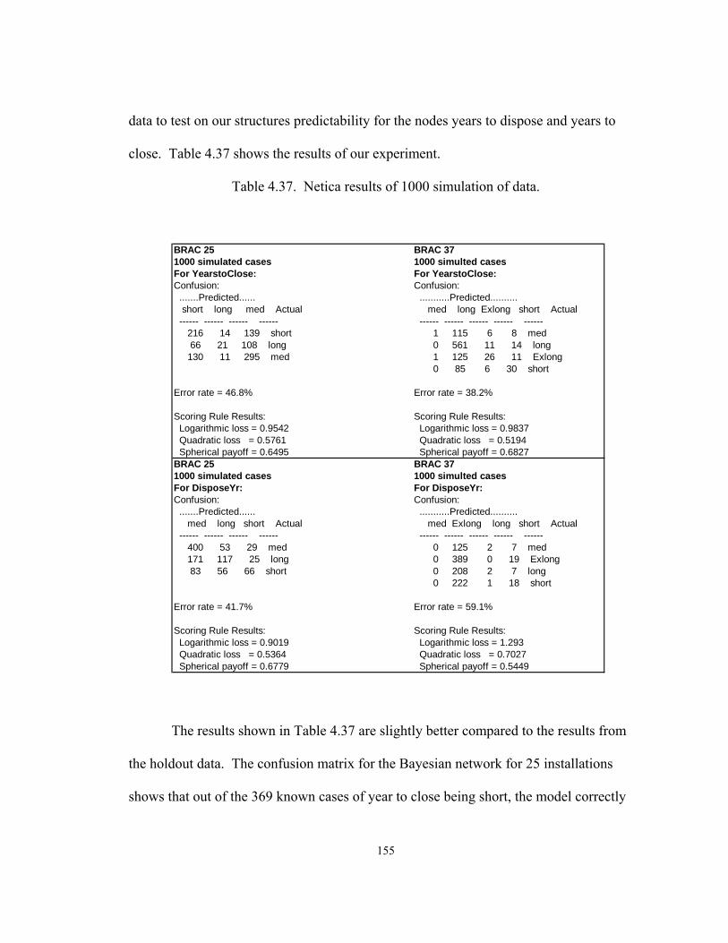
155
data to test on our structures predictability for the nodes years to dispose and years to
close. Table 4.37 shows the results of our experiment.
Table 4.37. Netica results of 1000 simulation of data.
BRAC 25 BRAC 371000 simulated cases 1000 simulted casesFor YearstoClose: For YearstoClose:Confusion: Confusion: .......Predicted...... ...........Predicted.......... short long med Actual med long Exlong short Actual ------ ------ ------ ------ ------ ------ ------ ------ ------ 216 14 139 short 1 115 6 8 med 66 21 108 long 0 561 11 14 long 130 11 295 med 1 125 26 11 Exlong
0 85 6 30 short
Error rate = 46.8% Error rate = 38.2%
Scoring Rule Results: Scoring Rule Results: Logarithmic loss = 0.9542 Logarithmic loss = 0.9837 Quadratic loss = 0.5761 Quadratic loss = 0.5194 Spherical payoff = 0.6495 Spherical payoff = 0.6827BRAC 25 BRAC 371000 simulated cases 1000 simulted casesFor DisposeYr: For DisposeYr:Confusion: Confusion: .......Predicted...... ...........Predicted.......... med long short Actual med Exlong long short Actual ------ ------ ------ ------ ------ ------ ------ ------ ------ 400 53 29 med 0 125 2 7 med 171 117 25 long 0 389 0 19 Exlong 83 56 66 short 0 208 2 7 long
0 222 1 18 short
Error rate = 41.7% Error rate = 59.1%
Scoring Rule Results: Scoring Rule Results: Logarithmic loss = 0.9019 Logarithmic loss = 1.293 Quadratic loss = 0.5364 Quadratic loss = 0.7027 Spherical payoff = 0.6779 Spherical payoff = 0.5449
The results shown in Table 4.37 are slightly better compared to the results from
the holdout data. The confusion matrix for the Bayesian network for 25 installations
shows that out of the 369 known cases of year to close being short, the model correctly

156
predicted short in only 216 (58.5%) of the cases. The error rate in predicting short was
greater than 60%. For predicting the other two categories the network did slightly better
for predicting medium years to close (67.6%) of the cases; but did worse for correctly
predicting long accurately. The prediction for the 37 installations performed even worse
for years to close in all categories except for long, with 95.7% correctly predicting the
cases. Overall the network for the 25 installations had an error rate of 46.8% for
predicting years to close and 41.7% error for years to dispose. The network with 37
installations improved the prediction rate for years to close but declined for years to
dispose as noted by the error rate and the logarithmic and quadratic loss scores. A
contributing factor to the error rate is due to the weak relationship between years to close
and dispose to the other nodes in the network as previously discussed.
To summarize the predictive data graphically we used a Receiver Operating
Characteristic (ROC) curve as we did similarly with the diabetes data. Figure 4.9 of a
Receiver Operating Characteristic (ROC) shows the results of testing the classification
accuracy of the model for 37 installations with 1000 cases. Our graph (Figure 4.10) does
not show overall accurate predictability as evaluated in the confusion matrix.
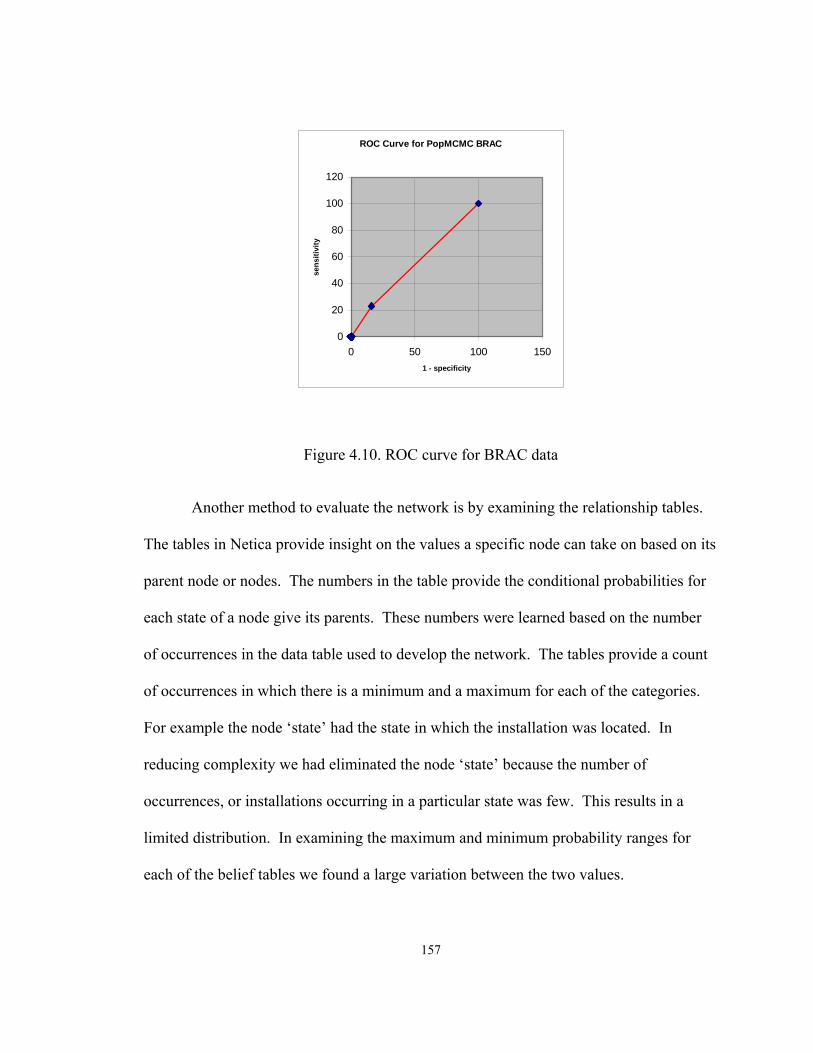
157
ROC Curve for PopMCMC BRAC
0
20
40
60
80
100
120
0 50 100 1501 - specificity
sens
itivi
ty
Figure 4.10. ROC curve for BRAC data
Another method to evaluate the network is by examining the relationship tables.
The tables in Netica provide insight on the values a specific node can take on based on its
parent node or nodes. The numbers in the table provide the conditional probabilities for
each state of a node give its parents. These numbers were learned based on the number
of occurrences in the data table used to develop the network. The tables provide a count
of occurrences in which there is a minimum and a maximum for each of the categories.
For example the node ‘state’ had the state in which the installation was located. In
reducing complexity we had eliminated the node ‘state’ because the number of
occurrences, or installations occurring in a particular state was few. This results in a
limited distribution. In examining the maximum and minimum probability ranges for
each of the belief tables we found a large variation between the two values.

158
We examined the minimum and maximum in each belief table in Netica for both
the BRAC networks with 38 and 36 variables. We focused on variations less than 15.
That is, if there was a difference of less than 15 between categories we assessed that
variable. We found the node ‘state’ we had eliminated varied the least of all the nodes
with a minimum probability of 5.56 and a maximum of 15.79 for the belief table. This is
because only a few states have installations. Similarly, the nodes that were collapsed,
MACOM and installation type also had minimal variation. The node PBTs also had a
small variation with a minimum probability of 22.58 and a max of 29.03. When we
reduced the number of nodes the probabilities associated with PBTs had a greater
variation between the min and max values. The new values became 8 and 60. Similarly,
installation type resulted in a minimum of 12.12 and a maximum of 57.58, a substantial
change from the previous network. It is notable that there were no variations less than 20
for the collapsed network. The lack of closeness in the probabilities allows us to state
with a greater degree of certainty a particular classification.
In the next chapter we will discuss future studies that could improve our process
of interleaving structure learning and discretization. From our work with sparse datasets
the approach of arc counting of the learned relationships to develop a structure may
provide a better structure as oppose to the structure with the highest BD score. This
approach was successful with the BRAC but further experimentation would be required.

159
5 Conclusions
Our research had set out with two main objectives: the first was an empirical
methods study of discretizing continuous variables interleaved with structure learning for
datasets with missing data; the second objective was to apply our methods to a problem
of significant interest to the Army. The problem of focus was the Base Realignment and
Closure (BRAC) process.
In our research we investigated four hypotheses within the framework of our two
main objectives. The first hypothesis evaluated the impact on interleaving discretization
with learning of structure to improve classification performance. We compared various
discretization methods interleaved with the learning algorithms to evaluate their relative
predictive performance. The discretization methods were evaluated using two methods
for learning structure, PopMCMC and BNPC for each of the datasets. The BNPC
process used a CI test to find relationships and performed slightly better than PopMCMC
for the less complex structures. However, for networks with more complexity and mixed
variables PopMCMC found more accurate structures. We had conjectured that the
interleaving of a discretization policy with learning would improve our learning of
Bayesian Networks. Previous research has shown that supervised discretization is better
than uninformed methods for learning structure [Monti, 99; Liu et al, 00]. We found that
the classification did improve using our process of discretizing with MCBD and learning

160
the structure with PopMCMC as we demonstrated in our experiment with the Iris and
Diabetes datasets.
We found that as the number of iterations was increased the accuracy of the
learned structure and the BD score for non-complex networks also improved. The
increase in iterations also resulted in great CPU time. We concluded that if accuracy is
more important than CPU time the increase in iterations could provide better results for
sparse networks. However, for more complex networks such as the Alarm network, the
CPU time becomes excessively long. The efficiency greatly deteriorated when we
increased the number of iterations from 100 to 1000 for complex datasets and the CPU
time increases by nearly 10 times. Methods to balance the efficiency and accuracy would
require further exploration beyond this work.
A further exploration of our inquiry was to examine the consequences of
introducing missing data on the performance of the aforementioned interleaving
approach. We found in comparing the scores of the learned structures that there is
minimal degradation as the percentage of missing data increases from 1 to 5 and finally
to 10 percent. We also noted that the missing data BD scores were similar to the BD
score without missing data. From our experiments we determined that when there is no
missing data, for a noncomplex network such as Asia, our process could find an accurate
structure to represent the dataset using discretization with structure learning.
As part of our research we applied interleaving discretization of continuous
variables with learning a BN to the BRAC historical data from 1988 to 1995. In our
previous experiments the smallest dataset we tested had 150 cases. After eliminating the

161
family housing locations, the BRAC dataset had only 41 installations, only 29 of which
were selected for closure prior to BRAC. Both datasets, 41 and 29 installations, 32% of
the data was missing. These datasets are so small as to seriously challenge any statistical
method.
We conclude from our experiments with the BRAC data that if there is a high
level of uncertainty associated with the data due to sparseness and unknown structure
then we should not settle on one structure as the best. To handle uncertainty when the
structure is unknown and the dataset is sparse we had hypothesized that combining
multiple models could result in more accurate inferences than a single ‘best’ model. An
approach we took to evaluate multiple models was to take the arc counts between the
nodes for all of the learned structures. Based on the highest counts between nodes we
used that information to build the model. From the arc count of all the best networks,
based on their BD score, was used to create a structure for evaluation in Netica. This
process found that the network provided accurate predictions on the years to close and
years to dispose. We found from our test that the model created from the arc counts
performed reasonably well to the single best model. The result of the experiment
provides an accurate predictor based on known evidence.
The BRAC 2005 Strategic Plan developed by the TABS office set the goal of
closing or realigning 60% of the installations within three years or less and disposing of
60% of the installations under six years. Our current evaluation of the BRAC data found
the four holdout installations fell within the desired category for closure but only one for
disposal. The cutpoints found by our process does not allow us to set the bins. The

162
cutpoints, as previously discussed were found through a search and score process.
However, the discretization policy found with the BN provided a means to evaluate
courses of action that could reduce the years to close or dispose of an installation. As
previously noted, we had suspected that the small data size and large number of variables
without strong relationships would produce multiple plausible BNs. Our process did find
a ‘good’ predictive network for the BRAC dataset through model averaging. Attaining
this objective in our study resulted in a model or models that can assist the BRAC
leadership in making decisions to achieve the BRAC goals and to investigate other
influences on base closure and disposition times.
Our process is an improvement over current methods, particularly methods that
incorporate inductive algorithms for learning which require all continuous variables to be
discretized in advance. Current methods use a one time preprocessing stage to fix the
partitions for subsequent learning. Preprocessing to discretize continuous variables may
not result in a network that represents the data. Poor discretization can mask underlying
relationships between variables as well as introduce spurious relationships.
The interleaving of discretization with structure learning we found in our study
provided variable interaction through global information sharing. Through the global
information sharing partitions were readjusted based on performance thresholds, in our
case the BD score. We had hypothesized that interleaving the two process would
improved our ability to model the underlying process that generated the data. The
structures learned with interleaving as tested did not provide the results we had thought
we could achieve as we noted in our evaluation of the Alarm and Sensor data. Similarly

163
we found the same results with the BRAC experiments. The results did provide several
models that allowed us to conduct more accurate responses to queries which we
compared to known facts on base closures, but overall, the models predictive capabilities
were complicated by the sparseness of the datasets. We would recommend further
evaluation to determine if other methods could improve model performance.
Based on a previous study of discretization [Xu, 03] and learning of structure
[Myers, 99] we had suspected the interleaving of MCMC with BD score with PopMCMC
for learning structure would perform better than the other methods. We had hypothesized
it would also be an improvement over current methods which primarily use discretization
as a preprocessing step to learning. In addition, we had suspected that the effects of
missing data on discretization policies would provide valuable insights on the amount of
degradation associated with missing data. From our analysis in this study noted when
missing data was less than 10% the degradation was minimal. However, we noted with
the increase of MAR the degradation also increased. We used our insights in our
evaluation of the BRAC data. The study used real world data from the BRAC process to
provide valuable insights to the decision makers in predicting the time for base closure
and disposition.
In conclusion, our research demonstrated the contribution of a stochastic process
for interleaving discretization and learning structure with missing data. Several methods
for learning structure with hidden variables and missing data exist [Friedman, 97]. There
are also numerous methods for discretization [Catlett, 91; Fayyad and Irani, 93;
Pfahringer, 95; Liu and Setiono, 95; Ho and Schott, 97]. Several authors have done

164
comparative analysis on discretization methods [Dougherty, et al, 95; Kohavi and
Sahami, 96; Liu, et al, 02]. Authors such as Friedman and Goldszmidt have dealt with a
combination of the issues: learning BNs with missing data or learning BNs with
continuous variables. However, to our knowledge and after extensive research we
conclude that this is the first time the problem of learning BN from data missing data and
continuous variable has been addressed together. Our study provides a method for
handling uncertainty found in sparse dataset that can provide a useful means for
inference.

165
APPENDIX A: BRAC datasets
COMPLETED INSTALLATIONS State State Zip Code
Closure / Realignme
nt
Congressional District1
(Number of Jurisdictions
Included)
EPA Region Acreage2 Excess
Acreage3SF Starting Inventory4
SF to be Disposed4 Installation Type5
1 Adelphi Woodbridge Res Fac VA 48 22191 CLOSURE 11 3 580 580 74,857 74,857 RDT&E/LABS*2 Alabama Ammunition Plant AL 1 35044 CLOSURE 3 4 2,235 2,235 381,977 381,977 Industrial3 Bayonne Military Ocean Terminal NJ 31 07002 CLOSURE 13 2 679 679 4,974,945 4,974,945 Industrial
*4 Big Coppett Key FL 10 33040 CLOSURE 20 4 5 5 2,586 2,586 Administration*5 Branch USDB, Lompoc CA 5 93436 CLOSURE 22 9 2,879 2,879 764,104 764,104 Administration6 Cameron Station VA 48 22304 CLOSURE 8 3 164 164 1,321,706 1,321,706 Administration
*7 Cape St. George FL 10 CLOSURE 0 4 6 6 0 0 Administration8 Coosa River Annex AL 1 35160 CLOSURE 3 4 2,836 2,836 349,580 349,580 Industrial9 Detroit Tank Plant MI 23 48090 REALIGN 12 5 342 153 1,137,981 1,137,981 Industrial
10 DMA Herndon VA 48 22066 CLOSURE 10 3 12 12 14,549 14,549 Administration11 DPSC Philadelphia PA 39 19145 CLOSURE 1 3 86 86 3,091,757 3,091,757 DLA12 East Fort Baker CA 5 94965 CLOSURE 6 9 91 91 267,391 267,391 Transport13 Fitzsimons AMC CO 6 80045 CLOSURE 6 8 578 557 2,901,325 2,809,139 Medical14 Ft Benjamin Harrison IN 15 46216 CLOSURE 6 5 2,514 2,370 4,908,379 4,638,379 Major Tng - Active15 Ft Chaffee AR 4 72095 CLOSURE 3 6 71,359 7,037 4,803,661 1,921,472 Major Tng - Active16 Ft Des Moines IA 16 CLOSURE 0 7 91 51 435,708 435,708 Administration17 Ft Devens MA 22 01432 CLOSURE 5 1 9,302 4,120 7,283,104 5,863,075 Major Tng - USAR
*18 Ft Dix NJ 31 08640 REALIGN 3 2 31,065 302 8,685,438 2,385,438 Major Tng - USAR19 Ft Douglas UT 46 84112 CLOSURE 2 8 119 51 778,710 300,789 Administration20 Ft Holabird MD 21 21222 CLOSURE 3 3 21 21 140,242 140,242 Hsg21 Ft Indiantown Gap PA 39 CLOSURE 0 3 17,797 570 4,030,143 1,313,687 Major Tng - USAR
*22 Ft Meade MD 21 20755 CLOSURE 5 3 13,309 8,470 9,541,647 0 Administration23 Ft Missoula MT 27 59801 CLOSURE 0 8 51 21 182,706 49,856 Administration24 Ft Sheridan IL 14 60037 CLOSURE 10 5 709 598 2,928,665 2,380,501 Administration
*25 Hingham Cohasset MA 22 CLOSURE 0 1 125 125 127,878 127,878 Administration26 Indiana AAP IN 15 47111 CLOSURE 9 5 10,650 859 4,767,759 0 Industrial27 Kapalama HI 12 96819 CLOSURE 1 9 21 21 822,317 822,317 Administration28 Kelly Support Center PA 39 15057 REALIGN 18 3 188 25 31,286 31,286 Administration29 Lexington-Bluegrass Army Depot KY 18 40516 CLOSURE 6 4 780 780 2,134,453 2,134,453 Depot30 New Orleans Mil Ocean Terminal LA 19 70143 CLOSURE 2 6 18 18 286,796 286,796 Industrial31 Nike Kansas City 30 MO 26 64070 CLOSURE 4 7 20 20 20,420 20,420 Administration32 Oakland Army Base CA 5 94626 CLOSURE 9 9 422 395 3,321,103 3,267,646 Industrial33 Pontiac Storage Facility MI 23 48342 CLOSURE 9 5 29 29 607,558 607,558 Industrial34 Presidio of San Francisco CA 5 94129 CLOSURE 8 9 1,480 1,480 6,517,426 4,617,426 Administration
*35 Recreation Center #2 Ft Bragg NC 34 28301 CLOSURE 8 4 4 4 17,035 17,035 Administration36 Red River Army Depot TX 45 75570 REALIGN 1 6 19,113 797 8,014,682 1,724,056 Depot
*37 Rio Vista USARC CA 5 94571 CLOSURE 3 9 28 28 72,825 72,825 Administration*38 Sudbury Training Annex MA 22 01776 CLOSURE 5 1 2,281 2,281 179,153 179,153 Administration39 Tooele Army Depot UT 46 84074 REALIGN 0 8 24,732 1,663 6,662,400 3,606,949 Depot
*40 USARC Gaithersburg MD 21 20877 CLOSURE 0 3 18 18 10,500 10,500 Administration41 Vint Hill Farms Station VA 48 20187 CLOSURE 10 3 696 696 1,262,406 1,262,406 Administration

166
MACOM Owner
MACOM owner tied
to an ID number
Number of
Mission Units
Number of
Civilian Employees before
BRAC
Number of
Military Employees before
BRAC
Local Populatio
n
Retiree Populatio
n
Local Unemplo
yment Before BRAC
Number of
Endangered
Species11
Superfund Site?
Amount of Power
Generation
Power generator
s meet local
standards?
Water Quality
Problems?
BRAC Round/Date
Closure Date
Final Transfer
AMC 3 NO DATA NO DATA NO DATA NO DATA NO DATA NO DATA 1 N NO DATA NO DATA NO DATA 07/10/1991 09/16/1994 06/26/1998AMC 3 Y 07/15/1988 12/30/1973 03/14/2003
MTMC 5 N 07/13/1995 09/30/1999 12/10/2002FORSCOM 4 N 07/13/1995 12/31/1988 06/29/2000FORSCOM 4 N 07/13/1995 12/31/1959 08/15/2002
MDW 7 N 07/15/1988 09/30/1995 12/06/1996FORSCOM 4 N 07/15/1988 02/28/1988 07/09/1993
AMC 3 N 07/15/1988 09/30/1992 10/11/1995AMC 3 N 07/15/1988 04/15/1999 12/07/2001MDW 7 N 07/15/1988 10/31/1993 03/17/1999DLA 9 N 07/02/1993 07/13/1999 10/05/2001
FORSCOM 4 N 07/15/1988 08/30/2000 08/01/2002MEDCOM 10 N 07/13/1995 06/30/1999 07/01/2003TRADOC 8 1 N 07/10/1991 09/30/1995 07/01/2002TRADOC 8 1 N 07/13/1995 09/27/1997 09/24/2003USARC 2 N 07/15/1988 09/30/1994 11/17/1999
TRADOC 8 1 Y 07/10/1991 03/31/1996 02/11/2003TRADOC 8 N 07/13/1995 10/01/1992 07/23/2003
#N/A N 07/15/1988 11/19/1991 11/19/1991MDW 7 N 07/13/1995 09/30/1995 02/12/2002
FORSCOM 4 N 07/13/1995 09/30/1998 09/01/1999MDW 7 Y 07/13/1995 10/30/1991 07/01/2002
FORSCOM 4 N 07/13/1995 07/30/2001 09/30/1999#N/A N 07/15/1988 05/27/1993 04/16/2001
FORSCOM 4 N 07/13/1995 12/31/1982 09/12/2003AMC 3 1 N 07/15/1988 08/31/1993 08/12/1993
USARPAC 6 N 07/15/1988 04/30/1993 09/30/1993FORSCOM 4 N 07/13/1995 05/26/2000 06/05/2003
AMC 3 N 07/15/1988 09/30/1991 09/30/1995MTMC 5 N 07/15/1988 11/30/1994 11/30/1994
#N/A N 07/15/1988 02/28/1988 08/05/2003MTMC 5 N 07/13/1995 09/30/1999 09/23/2003AMC 3 N 07/15/1988 10/30/1992 06/30/1994
FORSCOM 4 N 07/15/1988 09/30/1994 10/01/1994FORSCOM 4 N 07/13/1995 12/31/1985 08/06/2003
AMC 3 N 07/13/1995 09/30/1998 05/01/2002FORSCOM 4 N 07/13/1995 07/31/1994 03/26/2003FORSCOM 4 N 07/13/1995 09/30/1992 03/31/2003
AMC 3 Y 07/02/1993 09/30/1995 05/28/2002USARC 2 N 07/15/1988 12/31/1986 04/15/1996INSCOM 1 N 07/02/1993 09/30/1997 05/22/2003
Estimated Cost to Closure
Actual Cost to Closure
Estimated Cost to Transfer
Actual Cost to
Disposition ($000)
Estimated Environm
ental Costs ($000)
Actual Environm
ental Costs ($000)
Local Unemployment
After Brac
Jobs Lost
Jobs Created
Recovery (percent)
BAH for O1 w/out
dependants% urban Unemployment %
MilconNO DATA NO DATA NO DATA 343,353 1,578 7,353 NO DATA #DIV/0! $1,031 99.6% 3.9%
48 4,102 71,000 #DIV/0! $603 59.0% 10.3% 79.729,289 19,513 2105 252 13% $1,329 100.0% 6.5% 79.7
133 #DIV/0! $1,606 99.9% 3.0% 05,553 #DIV/0! $1,072 95.7% 9.3% 0
158,678 311 5,817 #DIV/0! $1,290 100.0% 3.2%#DIV/0! $669
72 332 #DIV/0! $603 52.8% 10.7%14,049 27 10,821 #DIV/0! $795 1.4
#DIV/0! $1,290 82.4% 1.3%1485 300 20% $1,083 100.0% 10.9%
15,601 3,675 #DIV/0! $1,331 92.7% 2.1% 11.952,690 23,856 1612 2169 135% $908 105.3
135,865 23,957 1050 815 78% $712 100.0% 4.8% 20610,519 1,256 26,980 352 #DIV/0! $586 9.6
269 #DIV/0! $727258,391 12,376 127,028 2178 2288 105% $1,216 85.9% 3.2% 160.280,859 10,889 1164 #DIV/0! $1,125 88.9% 6.5% 11.64,245 2,553 #DIV/0! $689 97.6% 5.8%
16,091 613 #DIV/0! $1,004 100.0% 6.3% 11.14,696 1,368 789 #DIV/0! $767 8.5
14,016 2,684 39,087 203 #DIV/0! $1,111 99.6% 7.8% 1.61,027 520 #DIV/0! $658 99.7% 7.5% 0.4
28,138 68,215 1681 0 0% $919 100.0%95 4,639 #DIV/0! $1,331 0
#DIV/0! $620 55.0% 5.5%14,977 74 #DIV/0! $1,623 96.5% 5.9%
1,742 209 #DIV/0! $805 52.0% 0.341,281 30,700 1131 838 74% $683 34.0%
2,406 #DIV/0! $7947,520 24,154 #DIV/0! $680 0.0% 3.6%
14,676 7,373 33,350 #DIV/0! $1,411 365725 277 #DIV/0! $795 100.0% 10.3%
100,720 217,880 3150 1980 63% $1,973 100.0% 4.6% 03 442 #DIV/0! $772 62.9% 2.6% 0
27,000 13,418 16,434 5654 #DIV/0! $669 66.9% 6.2% 7.25,348 #DIV/0! $1,516 77.6% 4.4% 0
500 5,588 21 #DIV/0! $1,661 90.0% 1.9% 0.824,419 5,509 24,618 1942 819 42% $689 86.0% 5.6% 73.7
#DIV/0! $1,290 100.0% 4.4%50,815 3,679 12,497 1472 344 23% $1,082 65.7% 2.7% 72.4

167
REFERENCES

168
REFERENCES
1. Allison, Paul D. Missing Data. Series: Quantitative Applications in the Social Sciences. Sage Publications, Inc. 2001.
2. Army BRACO. After Action Review: 1988-2001. 3. Army BRAC Office. Strategic Plan for the Army Implementation of BRAC 2005.
Washington, D.C., 2004. 4. Aubuchon, Vaughn, “Blood Pressure Chart.”http://www.vaughns-1-
pagers.com/medicine/blood-presssure.htm 5. Barron, Andrew, Jorma Rissanen, and Bin Yu. The minimum description length principle
in coding and modeling. (Special Commemorative Issue: Information Theory: 1948-1998) IEEE. Trans. Inform. Th., Oct, 2743-2760.
6. Bay, S. D. Multivariate discretization of continuous variables for set mining. In
Proceedings of the Sixth ACM SIGKDD International Conference on Knowledge Discovery and Data Mining (2000), pp. 315--319.
7. Beinlich I., H.Suermondt, H. Chavez, and G. F. Cooper. The ALARM Monitoring System:
A Case Study with Two Probabilistic Inference Techniques for Belief Networks. In 2nd Conference of AI in Medicine Europe, pages 247-256, London, England, 1989.
8. Binder, J., D. Koller, S. Russel, and K. Kanazawa. Adaptive Probabilistic Networks with
Hidden Variables. Machine Learning, 1997. 9. Bouckaert, Remco R. Properties of Bayesian belief network learning algorithms.
Proceedings Tenth Conference in Uncertainty in Artificial Intelligence. DeMantaras R, Poole D, editors. San Francisco, CA: Morgan Kaufmann; pp. 102-109, 1994.
10. Bouckaert, R. Probabilistic network construction using the minimum description length
principle. Proceedings European Conference on Symbolic and Quantitative Approaches to Reasoning and Uncertainty. Clarke M, Kruse R, Moral S, editors. New York: Springer-Verlag; pp. 41-48, 1993,
< http://citeseer.nj.nec.com/bouckaert93probabilistic.html >.

169
11. Boutilier, Craig, N. Friedman, M. Goldszmidt, and D. Koller. Context-specific independence in Bayesian networks. In Proceedings of the Twelfth Conference on Uncertainty in Artificial Intelligence (1996), pp. 115-- 123.
< http://citeseer.nj.nec.com/context/9968/4780 > 12. Boyen, Xavier and Daphne Koller. Tractable Inference for Complex Stochastic
Processes. In Proceedings of the Fourteenth Annual Conference on Uncertainty in Artificial Intelligence, (UAI-98), Cooper G and Moral S editors, pp.33-42, 1998.
< http://citeseer.nj.nec.com/1780.html > 13. Boyen, Xavier, Nir Friedman and Daphne Koller. Discovering the Hidden Structure of
Complex Dynamic Systems. In Proceeding of the Fifteenth Conference on Uncertainty in Artificial Intelligence, (UAI-99), K. Laskey and H. Prade, editors, pp.91-100. 1999.
< http://robotics.stanford.edu/~xb/uai99/ > 14. BRAC Lesson Learned and Other Reference Document Compilation: Summary of Key
Lessons Learned from Prior BRAC Rounds. 15 January 2004. 15. Bradley-Carter, Dane and Ajit Narayanan. Genetic Algorithms for Knowledge Discovery
in Continuous Data. 16. Brijs, Tom and Koen Vanhoof, Cost-sensitive Discretization of Numerous Attributes.
Proceedings of the Second European Symposium on Principles of Data Mining and Knowledge Discovery,. Nantes, France, Sep 1995.
17. British-American Tobacco Company. TABLE 2C;Percentage of Regular Cigarette
Smokers of Both Sexes in the Total Population 15 years of age and over; according to the number of cigarettes smoked per day; by age group. CANADA; 1965 1970 1972.1972.
18. Brown, Barbara G. Verification of Precipitation Forecasts: A Survey of Methodology
(Part II: Verification of Probability Forecasts at Points). <www.bom.gov.au/bmrc/wefor/staff/eee/verif/QPF_Prague2001/papers/bgb_paper_final.pdf>
19. Brown, David P. An Investigation into the use of Bayesian Networks in Probabilistic
Modeling and Simulation. George Mason University, Ph.D., 2004. 20. Carlin, Bradley P. and Thomas A. Louis. Bayes and Empirical Bayes Methods for Data
Analysis, 2nd Edition, Chapman & Hall/CRC, Boca Raton, FL, 2000. 21. Catlett, J. On Changing Continuous Attributes into Ordered Discrete Attributes. In Y.
Kodratoff, editor, Machine Learning (EWSL-91), European Working Session on Learning, pp. 164-178, Berlin, Germany, 1991.

170
22. Chang, K. C., and Kathryn Laskey. Sensor Fusion BN Model. George Mason University. 23. Charniak, Eugeane. Bayesian networks without tears. AI Magazine (winter 1991),
12(4),50-63. 24. Cheeseman P. and J. Stutz. Bayesian Classification (AutoClass): Theory and Results. In
U.M. Fayyad, G. Piatetsky-Shapiro, P. Smyth, and R. Uthurasamy, editors, Advances in Knowledge Discovery and Data Mining. MIT Press, 1996.
25. Cheng, Jie., Bell, David, Liu, W., An algorithm for Bayesian network construction from
data. (proceedings of the 6th International Workshop on Artificial Intelligence and Statistics, 1997) AI&STAT'97
26. Cheng J. and R. Greiner, "Comparing Bayesian network classifiers," in Proceedings of
the Conference on Uncertainty in artificial intelligence (UAI), 1999, pp. 101--108. 27. Cheng, J., Bell, D., and Liu, W. Learning bayesian networks from data: An efficient
approach based on information theory. Tech. Rep. -, Department of Computer Science - University of Alberta, 1998.
28. Chickering DM and D Heckerman. Efficient approximations for the marginal likelihood
of Bayesian networks with hidden variables. Mach. Learn., 29:181-212, 1997. 29. Chickering D., D. Heckerman, and C. Meek. A Bayesian approach to learning Bayesian
networks with local structure. In UAI '97, pages 80--89, 1997. 30. Ching, John Y., Andrew K. C. Wong, and Keith C. C. Chan, Class-Dependent
Discretization for Inductive Learning from Continuous and Mixed-Mode Data. IEEE Transactions on Pattern Analysis and Machine Intelligence, Vol. 17, No. 7, pp. 641-651, July 1995.
31. Chmielewski, Michal R. and Jerzy W. Grzymala-Busse. Global Discretization of
Continuous Attributes as Preprocessing for Machine Learning. International Journal of Approximate Reasoning, Vol. 15, No. 4, November 1996.
32. Chun-Nan Hsu, Hung-Ju Huang, Tzu-Tsung Wong: Implications of the Dirichlet Assumption for Discretization of Continuous Variables in Naive Bayesian Classifiers. Machine Learning 53(3): 235-263 (2003).
33. Clarke, Ellis, and Bruce A. Barton. Entropy and MDL Discretization of Continuous
Variables for Bayesian Belief Networks. International Journal of Intelligent Systems, Vol. 15, pp. 61-92, 2000.

171
34. Cobb, Barry R., Rafael Rumi, and Antonio Salmeron. Bayesian Network Models with Discrete and Continuous Varibles. Advances in Probabilistic Graphical Models, Vol. 214/2007, pp.81-102, 2007.
35. Cohen, Jacob. The Cost of Dichotomization. Applied Psychological Measurement, pp.
249-253, Issue: V7, 1983. 36. Cowell, Robert G. Parameter Learning from Incomplete Data for Bayesian Networks.
City University, London, England, unpublished, 1999. www.staff.city.ac.uk/~rgc/webpages/aistats99.pdf
37. Cooper G. F. The computational complexity of probabilistic inference using Bayesian
belief networks, Artificial Intelligence, (1990) 42, pp. 393-405. 38. Cooper, Gregory F. A Bayesian Method for Learning Belief Networks that Contain
Hidden Variables. Journal of Intelligent Information Systems, vol 4, pp. 71-88, 1995. 39. Cooper, Gregory, and E. Herskovits. A Bayesian method for the induction of probabilistic
networks from data. Machine Learning, Vol. 9, pp. 309-347, 1992. Kluwer Academic Publishers, Boston, MA.
40. Cooper, Gregory F. and Changwon Yoo. Causal Discovery from a Mixture of
experimental and Observational Data. In Proceeding of the Fifteenth Conference on Uncertainty in Artificial Intelligence, (UAI-99), K. Laskey and H. Prade, editors, pp.116-1125. 1999.
< http://citeseer.nj.nec.com/cooper99causal.html > 41. Cover, Thomas M and Joy A. Thomas. Elements of information theory. New York: John
Wiley & Sons; 1991. 42. Davies, Scott and Andrew Moore. Mix-nets: Factored Mixtures of Gaussians in Bayesian
Networks with Mixed Continuous and Discrete Variables. In Proceedings of the Sixteenth Annual Conference on Uncertainty in Artificial Intelligence, (UAI-00), pp. 168-175, 2000.
43. DeGroot, Morris H. Probability and Statistics. Second Ed. Addison-wesley Publishing
Co., Reading, MA, 1989. 44. Doll R, Hill AB. The mortality of doctors in relation to their smoking habits. British
Medical Journal 1954; 1:1451-1455. 45. Doll, Richard, Richard Peto, Jillian Boreham and Isabelle Sutherland. Mortality in
Relation to Smoking: 50 years’ Observations on Male British Doctors. British Medical Journal 2004; 328:1519-33.

172
46. Domingos, P. and Pazzani, M. (1997) On the Optimality of the Simple Bayesian Classifier under Zero-One Loss. Machine Learning, 29,103-130.
47. Dougherty J., R. Kohavi, and M. Sahami. Supervised and unsupervised discretization of
continuous features. In A. Prieditis and S. Russell, editors, Proc. Twelfth International Conference on Machine Learning, pages 194-202. Morgan Kaufmann, 1995,
< http://citeseer.nj.nec.com/dougherty95supervised.html >. 48. Duda, Richard O., Peter E. Hart, and David G. Stork. Pattern Classification. Second
Edition. John Wiley and Sons, Inc, 2001. 49. Everitt, Brian S., Sabine Landau and Morven Leese. Cluster Analysis, Fourth Edition.
Oxford University Press, Inc. NY, NY. 2001. 50. Faber, Vance. Clustering and the Continuous k-Means Algorithm. Los Alamos Science,
No. 22, pp. 138-144, 1994. 51. Fayyad, U. M., and Irani, K. B. (1993). Multi-interval discretization of continuous-valued
attributes for classification learning. Proceedings of the Thirteenth International Joint Conference on Artificial Intelligence (pp. 1022-1027). San Francisco, CA: Morgan Kaufmann.
52. Ferguson, Thomas S. A Bayesian Analysis of Some Nonparametric Problems. The Annals of Statistics, Vol. 1, No. 2(Mar., 1973), 209-230.
53. Frank, Eibe and Ian H. Witten. Making Better Use of Global Discretization. In
Proceedings of the Sixteenth International Conference on Machine Learning. Bled, Sovenia, 1999.
54. Friedman, Nir. Learning Belief Networks in the Presence of Missing Values and Hidden
Variables. Proceeding of the 14th International Conference on Machine Learning, (ICML-97), Vanderbilt University, Morgan Kaufmann Publishers, 1998.
55. Friedman, Nir. The Bayesian Structural EM Algorithm. In Proceedings of the 14th
Conference on Uncertainty on Artificial Intelligence, (UAI-98), 1998. 56. Friedman, N., D. Geiger, and M. Goldszmidt. Bayesian network classifiers. Machine
Learning, 29:131--163, 1997. < http://citeseer.nj.nec.com/context/790/129890 > 57. Friedman, N. and M. Goldszmidt. Discretizing continuous attributes while learning
Bayesian networks. In Machine Learning: Proceedings of the International Conference, 1996.
< http://citeseer.nj.nec.com/friedman96discretizing.html >.

173
58. Friedman, N. and M. Goldszmidt (1998). Learning Bayesian networks with local structure. In Learning in Graphical Models, pp. 421-460. Kluwer,
< http://citeseer.nj.nec.com/friedman96learning.html >. 59. Friedman, N., Moises Goldszmidt and Thomas J. Lee. Bayesian Network Classification
with Continuous Attributes: Getting the Best of Both Discretization and Parametric Fitting. In the Proceedings of the 15th International Conference on Machine Learning, (ICML-98), 1998.
60. Friedman, N., Devin Murphy and Stuart Russell. Learning the Structure of Dynamic
Probabilistic Networks. Fourteenth Conf. on Uncertainty in Artificial Intelligence (UAI). 1998. pp. 139-147.
61. Gama, J., Torgo, L., and Soares, C. Dynamic discretization of continuous attributes. In
Proceedings of the Sixth Ibero-American Conference on AI (1998), pp. 160--169. 62. Gamerman, Dani. Markov Chain Monte Carlo, Stochastic Simulation for Bayesian
Inference. Chapman and Hall, NY, NY, 2002. 63. GAO, The Report of the Department of Defense on Base Realignment and Closure, April
1998.
64. Geiger, Dan and David Heckerman. A Characterization of the Dirichlet Distribution through Global and local Parameter Independence. The Annals of Statistics, Vol. 25, No. 3 (Jun., 1997), 1344-1369.
65. Gelman, Andrew and Donald B. Rubin. Inference from Iterative Simulation Using
Multiple Sequences. Statistical Science, Vol. 7, Issue 4, pp. 457-472, Nov. 1992. 66. Gilks, W. R., A. Thomas, and D. J. Spiegelhalter, A Language and Program for Complex
Bayesian Modelling. The Statistician, 43: 169-78, 1994. < http://www.jstor.org> 67. Grzymala-Busse Jerzy W., Ming Hu: A Comparison of Several Approaches to Missing
Attribute Values in Data Mining. Rough Sets and Current Trends in Computing 2000: 378-385.
68. Hand, D. J., F. Daly, A. D. Lunn, K. J. McConway and E. Ostrowski. A Handbook of
Small Data Sets. Chapman and Hall, NY. NY., 1994. 69. Harris, John K, Gregory S. Parnell, et al.: Army BRAC 2005 Implementation.
unpublished. West Point, NY, June 2004.

174
70. Harris, John K, Gregory Parnell, et al.: A Decision Tool to Address the Army’s BRAC 2005 Implementation Challenges. ORCEN Technical Report [DSE-TR-0409], United States Military Academy, West Point, NY, May 2005.
71. Hastings, WK., Monte Carlo sampling methods using Markov chains and their
applications, j-biometrika Vol 57 No 1 pp 97-109, 1970. 72. Heckerman, D. Probabilistic Similarity Networks. PhD thesis, Program in Medical
Information Sciences, Stanford University, Stanford, CA, 1990. Report STAN-CS-90-1316.
73. Heckerman D. and J. Breese. Causal independence for probability assessment and
inference using Bayesian networks. Technical Report MSR-TR-94-08, Microsoft Research, 1995.
74. Heckerman, D. and Geiger, D. (December, 1994). Learning Bayesian networks.
Technical Report MSR-TR-95-02, Microsoft, < http://citeseer.nj.nec.com/context/544038/75203 >. 75. Heckerman, David. A tutorial on learning Bayesian networks. Technical Report MSR-
TR-95-06, Microsoft Research, Redmond, WA, March 1995, revised July 1995, < http://citeseer.nj.nec.com/135897.html >. 76. Heckerman, David. Bayesian Networks for Data Mining. Data Mining and Knowledge
Discovery 1, pp.79-119, Kluwer Academic Publishers, 1997. 77. Heckerman, D., Dan Geiger, and David M. Chickering. Learning Bayesian networks: the
combination of knowledge and statistical data. Machine Learning, 20, pp. 197-243, Kluwer Academic Publishers, Boston, MA, 1995.
78. Heckerman D., C. Meek, and G. Cooper. A Bayesian approach to causal discovery.
Technical Report MSR-TR-97-05, Microsoft Research, 1997. 79. Ho, K. M. and P. D. Scott. Zeta: A Global Method for Discretization of Continuous
Variables. Knowledge Discovery and Data Mining, 1997. 80. Hoeting, J. A., Madigan, D., Raftery, A. E. and Volinsky, C. T. (1999). Bayesian Model
Averaging. Statistical Science, 1999, Vol. 14, No 4, pp. 382-417. 81. Hofmann R. and V. Tresp, "Discovering Structure in Continuous Variables using
Bayesian Networks," Advances in Neural Information Processing Systems, vol. 8, 1995. 82. Holte, Robert C. Very Simple Classification Rules Perform Well on Most Commonly
Used Datasets. Machine Learning, Vol 11, pp. 63-91, 1993.
175
83. Holman, Barry, J. Reifsnyder, K. Kuhlman, and R. Irving. Status of Prior Base Realignment and Closure Rounds. GAO, December 1998.
84. Hong, S. J. Use of contextual information for feature ranking and discretization. IEEE
Transactions on Knowledge and Data Engineering, 9(5), pp. 718-730, 1997. 85. Hsu C.-N., H.-J. Huang, and T.-T. Wong, "Why Discretization Works for Naive Bayesian
Classifiers," Proc. 17th Int'l Conf. Machine Learning, pp. 399-406, 2000. 86. Hsu C.-N., H.-J. Huang, and T.-T. Wong, "Why Discretization Works for Naive Bayesian
Classifiers," Proc. 17th Int'l Conf. Machine Learning, pp. 399-406, 2000. 87. Hudson L.D., B.S. Ware, and S.M. Mahoney, Kathryn Blackmond Laskey: Antiterrorism
Risk Management for Military Planners George Mason University Homeland Security and Military Transformation Laboratory.
88. Ide S. and F. G. Cozman. Random generation of Bayesian networks. In Brazilian
Symposium on Artificial Intelligence, Recife, Pernambuco, Brazil, 2002.
89. Ide J.S. and F.G. Cozman. Testing MCMC algorithms with randomly generated Bayesian networks. Workshop de Teses e Dissertações em IA (WTDIA2002), Recife, Pernambuco, Brazil, 2002.
90. Jensen, Finn V. An Introduction to Bayesian Networks. Springer-Verlag New York, Inc.
New York, NY, 1998. 91. Jensen, Finn V. and Steffen L. Lauritzen. Probabilistic Networks. Handbook of
Defeasible Reasoning and Uncertainty Management Systems. D. M. Gabbay and Ph. Smets (eds.). Vol 5, pp. 289-320. Kluwer, Netherlands, 2000.
92. John, G., and Langley, P. (1995) Estimating Continuous Distributions in Bayesian
Classifiers. In Proceedings of the Eleventh Conference on Uncertainty in Artificial Intelligence, Morgan Kaufmann Publishers, San Mateo.
93. Kanungo,T, D. M. Mount, N. S. Netanyahu, C. Piatko, R. Silverman, and A. Y. Wu. The
Analysis of a Simple K-Means Clustering Algorithm. Proc. of ACM Symposium on Computational Geometry, Hong Kong, June 12-14, 2000
94. Kaufman, Kenneth A., and Ryszard S. Michalski. A Method for Reasoning with Structured and Continuous Attributes in the INLEN-2 Multistrategy Knowledge Discovery System. Proceedings of the Second International Conference on Knowledge Discovery and Data Mining (KDD-96), Portland OR, August 2-4, 1996, pp. 232-237.
176
95. Kayaalp, M., and Cooper, G. F.: A Bayesian Network Scoring Metric That Is Based on Globally Uniform Parameter Priors. Proceedings of the Eighteenth Annual Conference on Uncertainty in Artificial Intelligence (UAI-2002).
96. Kennett, R., K. Korb, and a. Nicholson, Seabreeze Predictions Using Bayesian Networks:
A Case Study. Proceedings of the 5th Pacific-Asia Conference on Advances in Knowledge Discovery and Data Mining –PAKDD, Springer-Verlag, New York, 2001.
97. Kerber, Randy. ChiMere: Discretization of Numeric Attributes. Proceedings, 10th
National Conference on Artificial Intelligence, (AAAI-92), pp. 123-128, AAAI Press, Menlo Park, CA, 1992.
98. Kohavi, Ron. A Study of Cross-Validation and Bootstrap for Accuracy Estimation and
Model Selection. In the International Joint Conference on Artificial Intelligence (IJCAI), 1994.
99. Kohavi R, and Sahami M (1996) Error-based and entropy-based discretization of
continuous features. Proceedings of the 2nd International Conference on Knowledge Discovery and Data Mining, pp. 114—119.
< http://citeseer.nj.nec.com/4084.html > 100. Kontkanen, Petri, Petri Myllymaki, Tomi Silander, and Henry Tirri. A Bayesian
Approach to Discretization. European Symposium on Intelligent Techniques, Bari, Italy, March 1997.
101. Kozlov, Alexander V, and Daphne Koller. Nonuniform Dynamic Discretization in Hybrid
Networks. In the Thirteenth Conference on Uncertainty in Artificial Intelligence (UAI-97) August 1-3, 1997, pp. 314-325.
< http://citeseer.nj.nec.com/kozlov97nonuniform.html> 102. Kurgan, Lukasz, and Krzysztof J. Cios. Discretization Algorithm that Uses Class-
Attribute Interdependence Maximization. 2001. < http://citeseer.nj.nec.com/kurgan01discretization.html> 103. Lachman, Beth, E. M. Pint, and D. Oaks. Lessons Learned from the Implementation of
Previous BRAC Decisions. RAND, Arroyo Center, AB 745-A, August 2003. 104. Lam, W., and Bacchus, F. Learning Bayesian belief networks: An approach based on the
MDL principle. Computer Intelligence, 10(3), pp. 269-293, 1994. 105. Lam, W. and Kon Fan Low. Using discretization and Bayesian inference network
learning for automatic filtering profile generation. IEEE Transactions on Systems, Man, and Cybernetics, Vol. 30, no. 3, pp. 340-351, August 2000.

177
106. Laskey, Kathryn Blackmond. Bayesian Decision Theory. Workshop conducted at SPARTA Corporation Annual Training Meeting, June 2002, Orlando, FL
107. Laskey, George, and Kathryn Laskey. Combat Identification with Bayesian Networks.
Presented at Command and Control Research and Technology Symposium 2002. 108. Laskey, Kathryn Blackmond and S. Mahoney. Network fragments: representing
knowledge for constructing probabilistic models. In Proceedings of the 13th Conference on Uncertainty in Artificial Intelligence (UAI-97), pages 334-- 341. Morgan Kaufmann, 1997.
< http://citeseer.nj.nec.com/context/28085/0>
109. Laskey, Kathryn Blackmond and James Myers. Population Markov Chain Monte Carlo 2003.. <http://ite.gmu.edu/~klaskey/publications.html>
110. Lauritzen S. L. and D. J. Spiegelhalter. Local computations with probabilities on
graphical structures and their application to expert systems. Journal of the Royal Statistical Society, Series B, 50(2):157--224, 1988.
111. Lauritzen, Steffen L. and Frank Jensen, Stable Local Computation with Conditional
Gaussian Distributions. Research Report R-99-2014, Department of Mathematical Sciences, Aalborg University, September 1999.
112. Lee, Peter M. Bayesian statistics, an introduction, 2nd edition. Oxford University Press
Inc., New York, NY, 1997. 113. Lepar, Vasilica and Prakash P. Shenoy. A Comparison of Lauritzen-Spiegelhalter, Hugin,
and Shenoy-Shafer Architectures for Computing Marginals of Probability Distributions. <http://citeseer.nj.nec.com/13252.html>
114. Lerner, Uri, Ronald Parr, Daphne Koller and Gautam Biswas. Bayesian fault detection
and diagnosis in dynamic systems. Proceedings of the Seventeenth National Conference on Artificial Intelligence (AAAI 2000), pp531-537.
115. Lindenbaum, Michael, Shaul Markovich and Dmitry Rusakov. Selective Sampling for
Nearest Neighbor Classifiers. Proceedings of the Sixteenth National Conference on Artificial Intelligence, (AAAI-99), pp. 366-371.
116. Liu H, and Setiono R (1995) Chi2: Feature selection and discretization of numeric
attributes. Proceedings of the 7th IEEE International Conference on Tools with Artificial Intelligence, pp. 388--391.
117. Liu, Huan, and Rudy Setiono. Feature Selection via Discretization. IEEE Transactions on
Knowledge and Data Engineering, Vol. 9, No. 4, pp. 642-645, July/August 1997.

178
118. Liu H., F. Hussain, C. L. Tan and M. Dash, "Discretization: An enabling technique", Journal of Data Mining and Knowledge Discovery Vol. 6, No. 4, 2002, pages 393 – 423.
119. Lucas, Peter: Bayesian Networks in Medicine: a Model-based Approach to Medical
Decision Making. paper on line at: http://citeseer.ist.psu.edu/cache/papers/cs/23583/http:zSzzSzwww.csd.abdn.ac.ukzSz~plucaszSzzSzeunite.pdf/bayesian-networks-in-medicine.pdf.
120. S. P. Lloyd, Least Squares Quantization in PCM,º IEEE Trans Information Theory, vol.
28, 129-137, 1982 121. MacKay D. Introduction to Monte Carlo Methods. In M. Jordan, editor, Learning in
graphical models. The MIT Press, Cambridge, Massachusetts, 1998. 122. Mackay D.J.C. (1995), Bayesian Methods for Neural Networks: Theory and Applications,
Course notes for Neural Networks Summer School. 123. Madigan D. and A. Raftery, Model selection and accounting for model uncertainty in
graphical models using Occam 's razor, Journal of the American Statistical Association 89 (1994), 1535--1546.
124. Madigan, D., A. Andersson, M. D. Perlman, and C. T. Volinsky. Bayesian Model
Averaging and Model Selection for Markov Equivalence Classes of Acyclic Digraphs. Communications in Statistics – Theory and Methods, 25(11):2493-2519, 1996.
125. Madigan, D, and J. York. Bayesian Graphical Models for Discrete Data. International
Statistical Review, 63:215-232, 1995. 126. Mahoney, Suzanne Mitchell. Network Fragments. PhD thesis, Information Technology
Program, George Mason University, Fairfax, VA, 1999. UMI number: 9925029. 127. McMichael, Daniel, Lin Liu, and Heping Pan. Estimating the Parameters of Mixed
Bayesian Networks from Incomplete Data. In Proceedings of Information Decision and Control 99, Adelaide, Australia, Feb 1999.
128. Monti, Stefano. Learning hybrid Bayesian networks from data. In M.I. Jordan (editor),
Learning in Graphical Models, pp. 521-540, Kluwer Academic Publishers, 1998. 129. Monti, Stefano. Learning hybrid Bayesian networks from data. PhD dissertation,
Intelligent Systems Program, University of Pittsburgh, Pittsburgh, PA, 1999. <www.cs.cmu.edu/~smonti/publications/phd.pdf>

179
130. Monti S. and G. F. Cooper. A Bayesian Network Classifier that combines a Finite Mixture Model and a Naive-Bayes Model. In Proceedings of 15th Conference of Uncertainty in AI (UAI-99), Stockolm, Sweden, 1999.
131. Monti S. and G. F. Cooper. A Multivariate Discretization Method for Learning Bayesian
Networks from Mixed Data. In Proceedings of 14th Conference of Uncertainty in AI (UAI-98), pages 404-413. Madison, WI, 1998.
132. Monti, S. and G. F. Cooper. (1999) A Latent Variable Model for Multivariate
Discretization. In Uncertainty 00: The seventh International Workshop on Artificial Intelligence and Statistics, Ft. Lauderdale, FL, January, 1999.
133. Murphy, Kevin P. Inference and Learning in Hybrid Bayesian Networks. U.C. Berkeley
Technical Report CSD-98-990, 1998. < http://www.cs.berkeley.edu/~murphyk/publ.html> 134. Murphy, Kevin P. A Variation Approximation for Bayesian Networks with Discrete and
Continuous Latent Variables. In Proceedings of 15th Conference of Uncertainty in AI (UAI-99), pp. 467-475, 1999.
135. Murphy K. Learning Bayes net structure from sparse data sets. Technical report, Comp.
Sci. Div., UC Berkeley, 2001. 136. Murphy Kevin. An introduction to graphical models. Technical report, Intel Research
Technical Report., 2001. paper at: http://www.ai.mit.edu/~murphyk/papers.html 137. Murphy, P. M. and Aha, D. W. (1994), UCI repository of machine learning databases,
http://[email protected] 138. Myers, James W. Stochastic Algorithms for Learning with Incomplete Data: An
Application to Bayesian Networks. PhD dissertation, Department of Systems Engineering, George Mason University, Fairfax, VA, 1999.
139. Myers James W., Kathryn B. Laskey, and Tod S. Levitt. Learning Bayesian networks
from incomplete data with stochastic search algorithms. In Proceedings of the Fifteenth Conference on Uncertainty in Arti cial Intelligence, pages 476-485. Morgan Kaufmann Publishers, 1999.<http://ite.gmu.edu/~klaskey/publications.html>
140. National Heart, Lung, and Blood Institute Growth and Health Study Research Group,
Obesity and cardiovascular disease risk factors in black and white girls: The NHLBI growth and health study. American Journal of Public Health, Vol. 82, pp. 1613-1620, December 1992.

180
141. Neal, Radford M. Probabilistic Inference Using Markov Chain Monte Carlo Methods. Toronto, University of Toronto, 1993.
142. Neapolitan, Richard E. Learning Bayesian Networks. Pearson Prentice Hall, Upper
Saddle River, NJ, 2004. 143. Nguyen, Hung Son. Rule Induction From Continuous Data, New Discretization
Concepts. In Proceedings of the 3rd Joint Annual Conference on Information Science, Raleigh, NC, 1997, Vol 3, pp. 81-84.
144. Nguyen, Hung Son, and Sinh Hoa Nguyen. Discretization Methods with Back-tracking,
1997. < http://citeseer.nj.nec.com/369995.html> 145. Pazzani, Michael J. An iterative improvement approach for the discretization of numeric
attributes in Bayesian classifiers. Proceedings First International Conference on Knowledge Discovery and Data Mining. Fayyad U. Uthurusamy R. editors. Menlo Park, CA: AAAI Press; pp. 228-233, 1995.
146. Pearl, Judea. Probabilistic Reasoning in Intelligent Systems: Networks of Plausible
Inference. Morgan Kaufmann Publishers, Inc, San Francisco, CA, revised second edition (2000), 1988.
147. Pearl, Judea. Causality: Models, Reasoning, and Inference. Cambridge University Press, 2000.
148. Pfahringer B. (1995). Compression-based discretization of continuous attributes. In
Proceedings of the Twelfth International Conference on Machine Learning, Morgan Kaufmann,
< http://citeseer.nj.nec.com/pfahringer95compressionbased.html > 149. Provost, Foster, T. Fawcett, and R. Kohavi. The case against accuracy estimation for
comparing induction algorithms. In Proceedings Fifteenth International Conference on Machine Learning, pages 445--453, Madison, WI, 1998. Morgan Kaufmann, San Francisco, CA.
150. Quinlan, J. R. Improved Use of Continuous Attributes in C4.5. Journal of Artificial
Intelligence Research, Vol. 4, pp. 77-90, 1996. 151. Ramoni M. and P. Sebastiani, "Discovering Bayesian networks in incomplete databases,"
Technical Report KMi-TR-46, Knowledge Median Institute, The Open University, March 1997. 231.

181
152. Riggelsen, Carsten and Ad Feelders. Learning Bayesian Network Models from Incomplete Data using Importance Sampling. Institute of Information and Computing Sciences, Utrecht University, The Netherlands.
153. Rissanen J. Stochastic complexity and modeling. The Annals of Statistics, 14(3):1080-
1100, 1986. paper available at www.isds.duke.edu/conferences/bath/rissanen.ps. 154. Russell, Stuart, and Peter Norvig. Artificial Intelligence, A Modern Approach. Prentice
Hall, Upper Saddle River, NJ, 1995. 155. Schairer, E. and E. Schoniger. Lung Cancer and Tobacco Consumption. International
Journal of Epidemiology, 2001; 30:24-27. Great Britian. 156. Singh, Moninder. Induction of Selective Bayesian Networks from Data. In Proceedings of
the 13th National Conf. on Artificial Intelligence (AAAI'96), Portland, Oregon, Aug. 4-8, 1371. Copyright 1996, AAAI.
157. Sivia, D. S. Data analysis a Bayesian tutorial, Oxford University Press, New York, NY,
2000.
158. Spiegelhalter, David J, and Lauritzen, S. L. Sequential updating of conditional probabilities on directed graphical structures. Networks 20 (1990), 579-605.
159. Spiegelhalter, David J, A. Philip Dawid, Tom A. Hutchinson and Robert G. Cowell.
Probabilistic Expert Systems and Graphical Modelling: A Case Study in Drug Safety. Philosophical Transactions: Physical Sciences and Engineering, Vol. 337, No. 1647, Complex Stochastic Systems (Dec. 15, 1991), 387-405.
160. Spiegelhalter, David J, A. Philip Dawid, Steffen L. Lauritzen and Robert G. Cowell,
Bayesian analysis in expert systems. Statistical Science, vol. 8, Issue 3(Aug. 1993), 219-247.
161. Spirtes, P., C. Glymour, and R. Scheines. Causality, Predictions and search. Springer-
Verlag, 1992. 162. Spirtes, P. and C. Meek. Learning Bayesian Networks with Discrete Variables from Data.
In Fayyad and Uthurusamy, 1995. 163. Sprites, P., Glymour,C. and Schienes, R. (1993) Causation, Prediction, and Search.
Springer- Verlag Lecture Notes in Statistics 81, Springer-Verlag, NY. 164. Ting, Kai Mi, Discretization of continuous-valued attributes and instance-based
learning, 1994. Technical Report 491, University of Sydney. <http://citeseer.nj.nec.com/ting94discretization.html>

182
165. Ventura, Dan. On Discretization as a Preprocessing Step for Supervised Learning Models. Masters Thesis, Department of Computer Science Brigham Young University, April 1995.
166. Ventura, Dan and Tony R. Martinez. An Empirical Comparison of Discretization
Methods. Proceedings of the Tenth International Symposium on Computer and Information Sciences, pp. 443-450, 1995.
167. Wang, Ke and Han Chong Goh. Minimum Splits Based Discretization for Continuous
Features. 168. Weiss, S and Indurkhya, N `Optimized Rule Induction' IEEE Expert Vol 8 No 6 (1993)
pp 61-69. 169. Wong, Andrew K. C., and David K. Y. Chiu. Synthesizing Statistical Knowledge from
Incomplete Mixed-Mode Data. IEEE Transactions on Pattern Analysis and Machine Intelligence, Vol. Pami-9, No. 6, pp. 796-805, Nov 1987.
170. Xu, Ning. A Comparison of Discretization Methods for Bayesian Networks. George
Mason University, Masters Thesis, 2003. 171. Yang, Ying, and Geoffrey I. Webb: A Comparative Study of Discretization Methods for
Naive-Bayes Classifiers, paper at: www.csse.monash.edu/~webb/cgi-bin/../Files/YangWebb02a.pdf

183
CURRICULUM VITAE
Pamela J. Hoyt was born on April 16, 1962, in Tecumseh, Michigan. She received her Bachelor of Arts from University of Vermont in 1984, her Masters of Science in Operations Research from George Mason University in 1996, and a Masters of Arts from U.S. Naval War College, 1999. She taught at the United States Military Academy, West Point as an Assistant Professor in the department of Systems Engineering 2002-2005. She is a Colonel in the U.S. Army and stationed at the Pentagon. She received her PhD in Information Technology in 2008.