discrete tire modeling for anti-lock braking system ... tire modeling for anti-lock braking system...
TRANSCRIPT

Discrete Tire Modeling for Anti-lock Braking System
Simulations
Srikanth Veppathur Sivaramakrishnan
Thesis submitted to the Faculty of the
Virginia Polytechnic Institute and State University
in partial fulfillment of the requirements for the degree of
Master of Science
in
Mechanical Engineering
Saied Taheri, Chair
Mehdi Ahmadian
Robert L. West
July 01, 2013
Blacksburg, Virginia
Keywords: Tire Modeling, ABS, Rigid Ring, Enveloping
Copyright 2013, Srikanth Veppathur Sivaramakrishnan
Discrete Tire Modeling for Anti-lock Braking System Simulations
Srikanth Veppathur Sivaramakrishnan
(ABSTRACT)
Tires play an extremely important role in the operation of a vehicle as they transmit forces
between the ground and the vehicle. Consistent efforts have been made over the years
towards modeling and simulation of tires and more recently, there has been an increasing
need to understand the transient response of tires to various high-frequency events such
as anti-lock braking and short-wavelength disturbances from the road. Major thrust has
been provided by the tire industry to develop simulation models that accurately predict the
dynamic response of tires without the use of computationally intensive tools such as FEA.
The objective of this research is to explain the development, implementation and validation
of a simulation tool based on a dynamic tire model that would assist in the analysis of the
effect of tire belt vibrations on the braking performance of a vehicle. A rigid ring tire model,
tandem elliptical cam enveloping model and a rule-based ABS model have been developed for
this purpose. These were combined together in a quarter vehicle model and implemented in
Matlab-Simulink R©. These models were developed for adaptation with CarSim R© to provide a
simulation tool that can be utilized in both tire and vehicle design processes. In addition to
model implementation, a parameterization procedure was developed to estimate the param-
eters of the rigid ring tire and enveloping model based on experimental data for a given tire.
Validation studies have also been performed to ensure the accuracy and validity of the tire
model. Following this, the braking performance of ABS under different road surfaces were
evaluated. Based on the simulation results, final conclusions were drawn with regards to the
analysis and detailed recommendations for future work directed towards the improvement of
the tool were provided.
This work was funded by the industry members of the Center for Tire Research (CenTiRe)

Dedication
To my parents and teachers who made me what I am today
iii

Acknowledgements
I would like to express my profound gratitude to my academic advisor and mentor Dr.Saied
Taheri for providing me the opportunity to work under his guidance at the Center for Tire
Research. His motivation kindled my passion for engineering research and his constant
support and timely advice played a huge role in completing my thesis. Dr.Taheri, it has
been an honor and great pleasure to work with you.
I would like to thank Dr.Mehdi Ahmadian and Dr.Robert West for their participation in
my thesis committee, and other faculty at Virginia Tech especially Dr.Pablo Tarazaga and
Dr.Steve Southward for their excellent courses which enhanced my technical skills in vibra-
tions and control.
I would also like to thank all the industry mentors of this project including Hankook Tires,
Michelin, Honda, Bridgestone etc. for their valuable comments and feedback throughout the
course of this study which kept the project moving in the right direction. A special mention
goes to all my lab-mates at CenTiRe especially to Ali for all the technical discussions, insights
and suggestions.
Finally, I want to acknowledge my roommates and all my friends who have been of immense
emotional support to me during my research and writing my thesis.
iv
Contents
List of Figures ix
List of Tables xiii
1 Introduction 1
1.1 Motivation . . . . . . . . . . . . . . . . . . . . . . . . . . . . . . . . . . . . . 2
1.2 Objective . . . . . . . . . . . . . . . . . . . . . . . . . . . . . . . . . . . . . 3
1.2.1 Model Requirements . . . . . . . . . . . . . . . . . . . . . . . . . . . 3
1.3 Research Approach . . . . . . . . . . . . . . . . . . . . . . . . . . . . . . . . 4
1.4 Thesis Outline . . . . . . . . . . . . . . . . . . . . . . . . . . . . . . . . . . . 5
2 Background 7
2.1 The Pneumatic Tire . . . . . . . . . . . . . . . . . . . . . . . . . . . . . . . 7
2.2 Tire Modeling . . . . . . . . . . . . . . . . . . . . . . . . . . . . . . . . . . . 8
2.2.1 Classification . . . . . . . . . . . . . . . . . . . . . . . . . . . . . . . 9
2.2.2 Empirical Tire Models . . . . . . . . . . . . . . . . . . . . . . . . . . 10
2.2.3 Physical Tire Models . . . . . . . . . . . . . . . . . . . . . . . . . . . 11
v

2.3 Anti-lock Braking Systems . . . . . . . . . . . . . . . . . . . . . . . . . . . . 17
2.3.1 Principle of Operation . . . . . . . . . . . . . . . . . . . . . . . . . . 19
2.3.2 ABS Control Algorithms . . . . . . . . . . . . . . . . . . . . . . . . . 20
2.4 Previous Work on Dynamic Tire Models with ABS . . . . . . . . . . . . . . 22
2.5 Conclusions . . . . . . . . . . . . . . . . . . . . . . . . . . . . . . . . . . . . 23
3 Mathematical Modeling 25
3.1 Dynamic Tire Model . . . . . . . . . . . . . . . . . . . . . . . . . . . . . . . 25
3.1.1 Assumptions . . . . . . . . . . . . . . . . . . . . . . . . . . . . . . . . 26
3.1.2 Coordinate System . . . . . . . . . . . . . . . . . . . . . . . . . . . . 27
3.1.3 Tandem Elliptical Cam Model . . . . . . . . . . . . . . . . . . . . . . 28
3.1.4 Rigid Ring Tire Model . . . . . . . . . . . . . . . . . . . . . . . . . . 30
3.2 Anti-lock Braking System Model . . . . . . . . . . . . . . . . . . . . . . . . 41
3.2.1 Inputs and Outputs . . . . . . . . . . . . . . . . . . . . . . . . . . . . 41
3.2.2 Assumptions . . . . . . . . . . . . . . . . . . . . . . . . . . . . . . . . 42
3.2.3 Brake States . . . . . . . . . . . . . . . . . . . . . . . . . . . . . . . . 43
3.2.4 ABS Control Cycling . . . . . . . . . . . . . . . . . . . . . . . . . . . 44
3.2.5 State Selection Rules . . . . . . . . . . . . . . . . . . . . . . . . . . . 44
3.2.6 Pressure Model . . . . . . . . . . . . . . . . . . . . . . . . . . . . . . 47
3.3 Quarter Car Model . . . . . . . . . . . . . . . . . . . . . . . . . . . . . . . . 48
3.4 Conclusions . . . . . . . . . . . . . . . . . . . . . . . . . . . . . . . . . . . . 49
vi
4 Implementation 50
4.1 Design Requirements . . . . . . . . . . . . . . . . . . . . . . . . . . . . . . . 50
4.2 Simulation Platform . . . . . . . . . . . . . . . . . . . . . . . . . . . . . . . 51
4.2.1 Simulink Modeling . . . . . . . . . . . . . . . . . . . . . . . . . . . . 51
4.3 Solvers and Time-steps . . . . . . . . . . . . . . . . . . . . . . . . . . . . . . 53
4.4 Data Exchange Standards . . . . . . . . . . . . . . . . . . . . . . . . . . . . 54
4.5 Model Optimization . . . . . . . . . . . . . . . . . . . . . . . . . . . . . . . 56
4.6 Conclusions . . . . . . . . . . . . . . . . . . . . . . . . . . . . . . . . . . . . 57
5 Model Parameterization 58
5.1 Reference Tire . . . . . . . . . . . . . . . . . . . . . . . . . . . . . . . . . . . 58
5.2 Experimental Procedure . . . . . . . . . . . . . . . . . . . . . . . . . . . . . 59
5.2.1 Nominal Parameters . . . . . . . . . . . . . . . . . . . . . . . . . . . 61
5.2.2 Inertial and Dimensional Parameters . . . . . . . . . . . . . . . . . . 61
5.2.3 Sidewall Stiffness and Damping . . . . . . . . . . . . . . . . . . . . . 62
5.2.4 Vertical Stiffness . . . . . . . . . . . . . . . . . . . . . . . . . . . . . 63
5.2.5 Effective Rolling Radius . . . . . . . . . . . . . . . . . . . . . . . . . 64
5.2.6 Contact Patch . . . . . . . . . . . . . . . . . . . . . . . . . . . . . . . 65
5.2.7 Rolling Resistance . . . . . . . . . . . . . . . . . . . . . . . . . . . . 65
5.2.8 Tread Element Stiffness . . . . . . . . . . . . . . . . . . . . . . . . . 67
5.2.9 Enveloping Characteristics . . . . . . . . . . . . . . . . . . . . . . . . 69
5.2.10 Alternative Methods of Parameterization . . . . . . . . . . . . . . . . 73
vii
5.3 Conclusions . . . . . . . . . . . . . . . . . . . . . . . . . . . . . . . . . . . . 74
6 Results and Validation 75
6.1 Enveloping Model Validation . . . . . . . . . . . . . . . . . . . . . . . . . . . 75
6.2 Tire Model Validation . . . . . . . . . . . . . . . . . . . . . . . . . . . . . . 78
6.3 Frequency Response to Brake Torque . . . . . . . . . . . . . . . . . . . . . . 84
6.4 ABS Simulations . . . . . . . . . . . . . . . . . . . . . . . . . . . . . . . . . 86
6.4.1 Test cases . . . . . . . . . . . . . . . . . . . . . . . . . . . . . . . . . 86
6.4.2 Vehicle Parameters . . . . . . . . . . . . . . . . . . . . . . . . . . . . 87
6.4.3 Simulation Results . . . . . . . . . . . . . . . . . . . . . . . . . . . . 87
6.5 Conclusions . . . . . . . . . . . . . . . . . . . . . . . . . . . . . . . . . . . . 90
7 Conclusions and Future Work 95
7.1 Recommendations for Future Work . . . . . . . . . . . . . . . . . . . . . . . 97
Bibliography 99
viii

List of Figures
1.1 Thesis outline. . . . . . . . . . . . . . . . . . . . . . . . . . . . . . . . . . . . 5
2.1 Detailed view of a pneumatic tire. Adapted from Zegelaar, P. (1998). The
dynamic response of tyres to brake torque variations and road unevennesses.
Delft University of Technology. Used under fair use, 2013. . . . . . . . . . . 8
2.2 Classification of tire models. Adapted from Pacejka, H. B. (2012). Tire and
Vehicle Dynamics (3rd ed.). Butterworth-Heinemann. Used under fair use,
2013. . . . . . . . . . . . . . . . . . . . . . . . . . . . . . . . . . . . . . . . . 10
2.3 Tire enveloping property. Adapted from Zegelaar, P. (1998). The dynamic
response of tyres to brake torque variations and road unevennesses. TU Delft.
Used under fair use, 2013. . . . . . . . . . . . . . . . . . . . . . . . . . . . . 12
2.4 Tire enveloping models. Adapted from Schmeitz, A. J. C. (2004). A Semi-
Empirical Three-Dimensional Model of the Pneumatic Tyre Rolling over Ar-
bitrarily Uneven Road Surfaces. Delft University of Technology. Used under
fair use, 2013. . . . . . . . . . . . . . . . . . . . . . . . . . . . . . . . . . . . 13
2.5 General classification of dynamic tire models. Adapted from Schmeitz, A.
J. C. (2004). A Semi-Empirical Three-Dimensional Model of the Pneumatic
Tyre Rolling over Arbitrarily Uneven Road Surfaces. Delft University of Tech-
nology. Used under fair use, 2013. . . . . . . . . . . . . . . . . . . . . . . . . 15
ix

2.6 Conventional vehicle braking system. . . . . . . . . . . . . . . . . . . . . . . 17
2.7 Bendix ABS System Schematic. . . . . . . . . . . . . . . . . . . . . . . . . . 18
2.8 General variation of tire longitudinal force with slip. . . . . . . . . . . . . . . 20
3.1 Global coordinate system. Adapted from Zegelaar, P. (1998). The dynamic
response of tyres to brake torque variations and road unevennesses. Delft
University of Technology. Used under fair use, 2013. . . . . . . . . . . . . . . 27
3.2 Tandem elliptical cam model. Adapted from Schmeitz, A. J. C. (2004). A
Semi-Empirical Three-Dimensional Model of the Pneumatic Tyre Rolling over
Arbitrarily Uneven Road Surfaces. Delft University of Technology. Used under
fair use, 2013. . . . . . . . . . . . . . . . . . . . . . . . . . . . . . . . . . . . 28
3.3 Rigid ring tire model. Adapted from Zegelaar, P. (1998). The dynamic re-
sponse of tyres to brake torque variations and road unevennesses. Delft Uni-
versity of Technology. Used under fair use, 2013. . . . . . . . . . . . . . . . . 31
3.4 Deformations in the tire. Adapted from Zegelaar, P. (1998). The dynamic
response of tyres to brake torque variations and road unevennesses. Delft
University of Technology. Used under fair use, 2013. . . . . . . . . . . . . . . 32
3.5 Tire-road contact model. Adapted from Zegelaar, P. (1998). The dynamic
response of tyres to brake torque variations and road unevennesses. Delft
University of Technology. Used under fair use, 2013. . . . . . . . . . . . . . . 37
3.6 ABS control cycling between different tires. . . . . . . . . . . . . . . . . . . . 45
3.7 Flowchart for the selection of brake states. . . . . . . . . . . . . . . . . . . . 46
3.8 Quarter car model. . . . . . . . . . . . . . . . . . . . . . . . . . . . . . . . . 48
4.1 Vehicle simulation model. . . . . . . . . . . . . . . . . . . . . . . . . . . . . 52
x
4.2 Tire model and enveloping model in Simulink. . . . . . . . . . . . . . . . . . 53
4.3 Rigid ring tire model in Simulink. . . . . . . . . . . . . . . . . . . . . . . . . 54
4.4 ABS subsystem. . . . . . . . . . . . . . . . . . . . . . . . . . . . . . . . . . . 55
4.5 Quarter car model in Simulink. . . . . . . . . . . . . . . . . . . . . . . . . . 55
5.1 Tire dimensions. Adapted from Zegelaar, P. (1998). The dynamic response
of tyres to brake torque variations and road unevennesses. Delft University of
Technology. Used under fair use, 2013. . . . . . . . . . . . . . . . . . . . . . 60
5.2 Loaded radius measurements at P = 2.2 bar. . . . . . . . . . . . . . . . . . . 64
5.3 Measurements at vertical deflection = 0.0128 m. . . . . . . . . . . . . . . . . 65
5.4 Effective rolling radius measurements at 2.2 bar . . . . . . . . . . . . . . . . 67
5.5 Contact patch length vs. vertical load at 2.2 bar. . . . . . . . . . . . . . . . 68
5.6 Variation of rolling resistance. . . . . . . . . . . . . . . . . . . . . . . . . . . 69
5.7 Steady-state force vs. slip characteristics. . . . . . . . . . . . . . . . . . . . . 70
5.8 Enveloping characteristics for multiple loads. . . . . . . . . . . . . . . . . . . 71
5.9 Enveloping model fit with experimental data. . . . . . . . . . . . . . . . . . 72
5.10 Tire FEA modeling. . . . . . . . . . . . . . . . . . . . . . . . . . . . . . . . 73
5.11 Procedure for parameter estimation. . . . . . . . . . . . . . . . . . . . . . . . 74
6.1 Enveloping over a cylindrical cleat at Fz = 2000 N. . . . . . . . . . . . . . . 76
6.2 Enveloping over a trapezoidal cleat at Fz = 4000 N. . . . . . . . . . . . . . . 76
6.3 Enveloping over a triangular cleat at Fz = 2000 N. . . . . . . . . . . . . . . 77
6.4 Tire rolling over a rectangular cleat at 20 km/h and Fz = 2000 N. . . . . . . 79
xi

6.5 Tire rolling over a rectangular cleat at 60 km/h and Fz = 2000 N. . . . . . . 80
6.6 Tire rolling over a rectangular cleat at 60 km/h and Fz = 4000 N. . . . . . . 81
6.7 Tire rolling over a rectangular cleat at 60 km/h and Fz = 6000 N. . . . . . . 82
6.8 Frequency response to brake torque input. . . . . . . . . . . . . . . . . . . . 85
6.9 Road profiles for ABS braking analysis. . . . . . . . . . . . . . . . . . . . . . 88
6.10 Braking distance on various road surfaces. . . . . . . . . . . . . . . . . . . . 90
6.11 ABS braking on smooth asphalt road. . . . . . . . . . . . . . . . . . . . . . . 91
6.12 ABS braking on jointed pavement concrete road. . . . . . . . . . . . . . . . . 92
6.13 ABS braking on ISO grade D poor asphalt road. . . . . . . . . . . . . . . . . 93
6.14 ABS braking on uneven road surface with cleats and potholes. . . . . . . . . 94
7.1 Simulation tool overview. . . . . . . . . . . . . . . . . . . . . . . . . . . . . . 96
xii

List of Tables
5.1 Reference tire notation . . . . . . . . . . . . . . . . . . . . . . . . . . . . . . 59
5.2 Measurements points for multiple loads and inflation pressures . . . . . . . . 60
5.3 Nominal parameters for the tire . . . . . . . . . . . . . . . . . . . . . . . . . 61
5.4 Geometric and inertial parameters of the tire . . . . . . . . . . . . . . . . . . 62
5.5 Estimated sidewall stiffness and damping . . . . . . . . . . . . . . . . . . . . 62
5.6 Estimated vertical stiffness parameters . . . . . . . . . . . . . . . . . . . . . 66
5.7 Estimated parameters for effective rolling radius . . . . . . . . . . . . . . . . 66
5.8 Estimated parameters for the contact patch . . . . . . . . . . . . . . . . . . 66
5.9 Estimated parameters for rolling resistance . . . . . . . . . . . . . . . . . . . 67
5.10 Estimated value of tread element stiffness . . . . . . . . . . . . . . . . . . . . 69
5.11 Estimated parameters for the enveloping model . . . . . . . . . . . . . . . . 72
6.1 Quarter car parameters . . . . . . . . . . . . . . . . . . . . . . . . . . . . . . 87
xiii
Chapter 1
Introduction
Rapid advancements in technology and computational ability to quickly solve differential
equations at affordable costs has led to widespread adoption of simulations for design in
the engineering industry, particularly in the automotive and tire sectors. Today, computer
simulations have become indispensable and are an integral part of any product design and
development process. The availability of an advanced and accurate simulation model is
considered a competitive advantage as this enables engineers to analyze multiple test cases
without experimentation and rapidly optimize their final product design. This also reduces
the cost of prototyping and improves product development time. Over the last few decades,
there have been numerous theories and models proposed, both from academia and industry
to simulate the behavior of various vehicle subsystems. This includes multiple modeling
approaches ranging from complex and computationally intensive Finite Element (FE) based
models to simplified lumped parameters discrete models. With each iteration, there has
been progress towards improving the accuracy of the simulations by validating the model
with experimental results. Realizing their importance, companies tend to invest considerable
effort towards developing in-house models for tires, vehicles and related safety systems for
their product development work-flow. Some of these models are considered trade secrets as
they served a critical purpose for their design. In addition to this, there are also companies
1

Srikanth Veppathur Sivaramakrishnan Chapter 1. Introduction 2
which exclusively develop simulation tools and commercially license such products to the
industry.
Although fairly advanced multi-body dynamics models exist for calculating the response of
the entire vehicle, modeling a pneumatic tire is considered a challenge because it is one of the
most complex components of a vehicle consisting of multiple structural elements. Early tire
models were merely simple mass-spring-dampers and were used for comfort and durability
studies. Over the years, advanced tire models have been developed which could predict the
dynamic response of the tire under various operating conditions and road inputs. Some of
these models require fairly high amount of computational capability.
1.1 Motivation
One of the most important application of tire and vehicle models is in the development of
safety systems such as Anti-lock Braking System (ABS) and Vehicle Stability Control (VSC)
which are essential features in all modern automobiles. As the control algorithms for these
systems become more advanced, there is a requirement to accurately predict and understand
the forces generated due to the dynamic response of the rolling tire due to road contact, short
wavelength road disturbances, brake torque variations and the interaction of the tire with the
vehicle. From the standpoint of the automotive manufacturer, this is important because tires
are responsible for transmitting forces from the ground to the vehicle for traction, braking
and steering. A deeper understanding of the factors governing the dynamic force response
of tires would provide immense scope towards evaluating and optimizing the performance of
their controllers. For the tire manufacturer, an ABS braking simulation model would assist
engineers in modifying their tire design to maximize braking performance.
In the current scenario, each tire and automotive manufacturer use their own in-house sim-
ulation code to evaluate ABS braking performance. Each model has its own disadvantages.
This is due to the fact that the tire manufacturers would not have access to commercial ABS

Srikanth Veppathur Sivaramakrishnan Chapter 1. Introduction 3
control algorithms and models since they are considered Intellectual Property (IP) and are
not revealed. Vehicle manufacturers lack the expertise of the tire industry in dynamic tire
models as these are also considered equally critical to protect. Due to the lack of a common
evaluation tool, engineers from both industries might not be able to target the same issue
and work towards a solution.
The need for such evaluation tools employing dynamic tire models have been validated
through previous studies by Pauwelussen [2] and Jansen [3] which conclusively state that the
effect of tire belt vibrations on ABS braking is significant and cannot be neglected.
1.2 Objective
The objective of this study is the develop a simulation tool that would serve as a common
platform for both tire and automotive manufacturers to analyze the effects of tire belt vibra-
tions, road disturbances and high frequency brake torque variations on the performance of
ABS in a vehicle. Once deployed into the industry, this tool could eventually be integrated
into the development work flow of engineers.
1.2.1 Model Requirements
Understanding the key requirements from the simulation model is essential to ensure proper
implementation of the tool. Developing the tool without complete knowledge of expected
features will lead to either spending unnecessary effort in modeling factors that are not
required or falling short of satisfying key requirements, which are listed below:
• The simulation tool should be capable of modeling the dynamic response of the tire
for excitations up to 100 Hz on any type of uneven road including short wavelength
disturbances and simulate all kinds of braking maneuvers.

Srikanth Veppathur Sivaramakrishnan Chapter 1. Introduction 4
• The model should be capable of calculating results at a relatively fast speed with low
computational effort.
• The simulation results should be accurate within the operating limitations of the mod-
els and verifiable through experiments.
• A parameterization procedure needs to be developed to ensure that the simulation tool
is capable of performing calculations for any general tire.
• The parameters required for the simulation model should be kept to a minimum with
low experimental effort required for parameter estimation.
• Standard formats should be adopted for the exchange of experimental data and tire
parameters for model parameterization and validation to avoid ambiguity and improve
integration into the existing design work-flow.
• The ABS algorithm should be based on a commercial ABS system installed in a pro-
duction vehicle with comparable performance and response.
• Implementation of the model should be done on a commonly used simulation platform
and should be capable of being adopted to other platforms or run as a standalone
application.
• The simulation tool should be capable of being adapted for real-time applications such
as Hardware-In-the-Loop (HIL) simulations.
• Tire and ABS models should be able to interface with commercial vehicle dynamic
software such as CarSim R©.
1.3 Research Approach
In order to fulfill the final objective, the work was divided into multiple tasks which would
serve as individual blocks that can be built upon towards the completion of the final model.

Srikanth Veppathur Sivaramakrishnan Chapter 1. Introduction 5
The following steps, which are explained in subsequent chapters in this thesis were taken
towards achieving the final objective:
• Comprehensive literature review of all the available tools and existing technology which
can be leveraged towards the development of the tool.
• Detailed mathematical modeling of all components based on a set of assumptions and
modeling requirements.
• Identification of simulation platform, implementation and integration of individual
models into larger simulation models.
• Development of estimation procedure to parameterize the tire model from experimental
data for model generalization.
• Detailed analysis of simulation results and their comparison with experimental data.
Literature
Review
Experimental
data
Mathematical
modeling
Model
parameterization
Simulation tool
implementation
Simulation results
and analysis
Conclusions and
future work
Figure 1.1: Thesis outline.
1.4 Thesis Outline
The chapters are organized in the same order as outlined in the research approach adopted in
this thesis. Chapter 2 provides a detailed background relating to all the models which were

Srikanth Veppathur Sivaramakrishnan Chapter 1. Introduction 6
implemented. Chapter 3 explains the mathematical modeling of the tire, vehicle and the
ABS model followed by the implementation of the tool which is further explained in Chapter
4. The procedure developed to estimate the parameters of the tire model is described in
Chapter 5. Detailed analysis of simulation results for various test cases are explained in
chapter 6. Final conclusions and recommendations for future work are provided in Chapter
7. Figure 1.1 illustrates the outline of this thesis.
Chapter 2
Background
This chapter provides a detailed overview of the state-of-the-art in the modeling and simu-
lation of automotive tires, braking systems and their integration with vehicle models from
published literature. The modeling and implementation of the tool components which are
explained in subsequent chapters are largely built upon the work detailed in the literature.
The rationale behind the choice of simulation models are explained here.
2.1 The Pneumatic Tire
In order to understand the behavior of a pneumatic tire, it is essential to understand its
construction. The tire is a composite element which is essentially a torus made of visco-
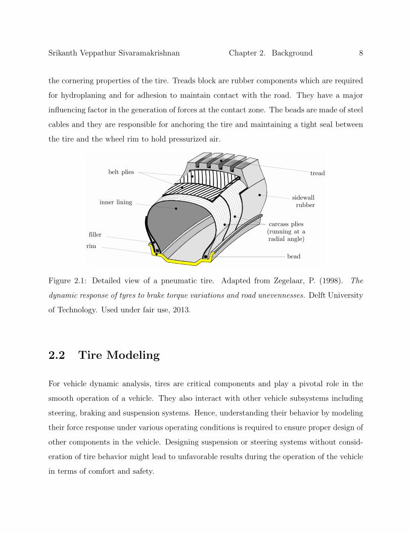
elastic rubber reinforced with high-tensile strength cords. Figure 2.1 shows the internal
composition of radial-ply tire. This tire has parallel cords, known as carcass plies running
from one bead to another. There are two stiff belts made of fabric and reinforced by steel
that runs around the circumference of the tire. The belt plies, typically aligned at 20deg to
the circumference and the pressurized sidewalls provide structural and directional stability
to the tires. The soft carcass provides for ride comfort and the stiff belts are essential for
7
Srikanth Veppathur Sivaramakrishnan Chapter 2. Background 8
the cornering properties of the tire. Treads block are rubber components which are required
for hydroplaning and for adhesion to maintain contact with the road. They have a major
influencing factor in the generation of forces at the contact zone. The beads are made of steel
cables and they are responsible for anchoring the tire and maintaining a tight seal between
the tire and the wheel rim to hold pressurized air.
Chapter 1
to the axle and further to the vehicle. The variations in normal load of the tyrehave an important, often adverse, effect on the generation of horizontal shearforces.
The behaviour of the pneumatic tyre is related to its complex construction, itcan be seen as a visco-elastic torus composed of high-tensile-strength cords andrubber. Figure 1.1 shows the construction of a radial-ply tyre which is the typicalconstruction of modern automobile tyres. The radial-ply tyre (in short radial tyre)is characterised by parallel cords running directly across the tyre from one beadto the other. These cords are referred to as the carcass plies. Directional stabilityof the tyre is supplied by the enclosed pressurised air acting on the sidewalls ofthe carcass and by a stiff belt of fabric or steel that runs around thecircumference of the tyre. The direction of the parallel plies of the belt isrelatively close to the circumferential: typically 20°.
tread
bead
filler
rim
carcass plies(running at aradial angle)
belt plies
inner liningsidewallrubber
Figure 1.1: Construction of a radial-ply tyre.
The relatively soft carcass provides the radial tyre with a soft ride and the stiffbelt provides the radial tyre with good cornering properties by keeping the treadflat on the road despite horizontal deflections of the tyre. The function of thetread is to establish and maintain contact between the tyre and the road. The keyfactor for the generation of horizontal forces in the contact zone is the adhesionbetween tread and road. The remaining components of the tyre are the steel-cablebeads which firmly anchor the assembly to the rim.
14
Figure 2.1: Detailed view of a pneumatic tire. Adapted from Zegelaar, P. (1998). The
dynamic response of tyres to brake torque variations and road unevennesses. Delft University
of Technology. Used under fair use, 2013.
2.2 Tire Modeling
For vehicle dynamic analysis, tires are critical components and play a pivotal role in the
smooth operation of a vehicle. They also interact with other vehicle subsystems including
steering, braking and suspension systems. Hence, understanding their behavior by modeling
their force response under various operating conditions is required to ensure proper design of
other components in the vehicle. Designing suspension or steering systems without consid-
eration of tire behavior might lead to unfavorable results during the operation of the vehicle
in terms of comfort and safety.

Srikanth Veppathur Sivaramakrishnan Chapter 2. Background 9
2.2.1 Classification
Tire modeling is an active area of research owing to its sheer complexity. Various theories
and methods were proposed towards modeling the behavior of tires. The type of tire model
used is heavily dependent on their targeted application which can span multiple domains
including material characterization, thermal response, strain mechanics and dynamics. The
primary focus of this section is towards tire models which can be used for vehicle dynamic
analysis. Based on the type of response, tire models can be classified as:
Steady-State Response A steady state condition is a situation in which there are low
variations in the input quantities to the tire (vertical load, slip). Some of the scenarios
that match this condition involve slow steering maneuvers such as cornering and lane
changing. Steady state tire models are the most widely used and can be both physical
and empirical.
Transient Response Steady state tire models lose their validity under conditions where are
rapid variations in slip with time. This is because the force generation in tire does not
instantaneously follow slip variations. The time constant of this response is described
using the concept of relaxation length which is defined as the distance traveled before
force generation in response to a step variation in slip. Transient tire models account for
the effect of relaxation length using various differential equations and predict the force
response more accurately at shorter time steps. In some methods, the transient effects
are calculated by physically modeling the tire mass in contact with the ground through
differential equations. Transient responses are mainly required under fast events such
as lane change at high velocities, ABS braking and traveling on a rough road to name a
few. Relaxation length is required to model the shimmy phenomenon [4] which occurs
on the front wheels of vehicles and also on the landing gear of aircraft.
According to H.B.Pacejka [5], tire models (both transient and steady state) can be broadly
classified into four categories, as shown in Figure 2.2. Each of these models have their own

Srikanth Veppathur Sivaramakrishnan Chapter 2. Background 10
advantages and shortcomings with varying levels of accuracy. The choice of model to be
used in this thesis is based on current modeling requirements. Some of the most important
tire models which fall into one of these categories are explained below:
2.5. TIRE MODELS (INTRODUCTORY DISCUSSION)
Several types of mathematical models of the tire have been developed duringthe past half-century; each type for a specific purpose. Different levels ofaccuracy and complexity may be introduced in the various categories ofutilization. This often involves entirely different ways of approach. Figure 2.11
degree of fit
number of fullscale tests
complexity of formulationseffort
insight in tyrebehaviour
number of special experiments
approach more
empirical theoretical
through simplephysical model
through complexphysical model
fitting full scaletyre test data by regression techniques
distorting,rescaling and combiningbasic characteristics
using simplemechanicalrepresentation,possibly closedform solution
describing tyrein greater detail, computer simulation, finite element method
e.g. Magic Formula
e.g. Brush model
e.g.RMOD-K. FTire
FIGURE 2.11 Four categories of possible types of approach to develop a tire model.
Exercise 2.3 Partial Differential Equations with Longitudinal Slip Included
Establish the differential equations for the sliding velocities similar to the Eqns
(2.58, 2.59) but nowwith longitudinal slip k included (a and 4 remain small). Note
that in that case Vr s Vc and that Vr may be expressed in terms of Vcx (zVc) and k.
Also, find the partial differential equations governing the deflections in the
adhesion zone similar to the Eqns (2.60, 2.61).
81Chapter | 2 Basic Tire Modeling Considerations
from experimental data only
using similarity method
Figure 2.2: Classification of tire models. Adapted from Pacejka, H. B. (2012). Tire and
Vehicle Dynamics (3rd ed.). Butterworth-Heinemann. Used under fair use, 2013.
2.2.2 Empirical Tire Models
These are mainly linear or non-linear mathematical relations which are derived based on
fitting experimental data. The biggest advantages of such models is their high accuracy
in predicting force response as their outputs are based on regressive analysis of previously
collected experimental data under similar conditions. Some their shortcomings are that
the equations formulated through this method are purely algebraic curves and have very

Srikanth Veppathur Sivaramakrishnan Chapter 2. Background 11
little physical significance as one cannot correlate the parameters of such models to the
actual properties of the tire. Also, parameterization of such models would require extensive
experimental data which can prove to be expensive.
Some of the most popular example of an empirical tire models is the Magic Formula by
Pacejka [6] which is considered a standard tire model in the industry for vehicle dynamic
simulations. The Magic Formula has been improved over the years with the addition of more
empirical relations to account for transients and inflation pressure changes [7, 8]. Braghin et
al proposed an extension to the Magic Formula by developing MF-Relax [9], which accounts
for the dynamic effects of the tire with a focus towards Anti-lock Braking System simulations.
2.2.3 Physical Tire Models
These are based on analytical derivations that are actually based on a set of assumptions
that would define the tire in a physical sense. The parameters of such models are based on
actual measurable entities of the tire such as belt mass, rotational moment of inertia, vertical
stiffness etc. Since these models are analytically derived, their outputs tend to have higher
scope in terms of analysis as one can correlate outputs to specific tire parameters. Hence,
they are extensively utilized during the design stage of the tire. The earliest application of
physical tire models were in ride and durability studies were the tire was a simple lumped
mass, spring and a damper. Such models are still being used to model vibration response
for both passive and active suspension design.
One of the most widely used physical models with a simplified formulation for vehicle dy-
namic studies is the HSRI model, also known as the ’brush model’ developed by Dugoff,
Francher and Segel [10] which was later improved by Bernard, Segel and Wild [11]. Some
of the recent advances in developing simple, unified physical models for all kinds of analysis
include UniTire [12]

Srikanth Veppathur Sivaramakrishnan Chapter 2. Background 12
Tire Enveloping Property
The behavior of a tire while rolling over obstacles is a complex phenomenon as the tire
is in contact with the ground at multiple points. This effect is clearly evident when the
road disturbances have short wavelengths as the tire contact creates a filtering effect by
smoothening out sharp obstacles. This is known as the enveloping property of the tire,
which is illustrated by Zegelaar [1] in Figure 2.3. As a result of the enveloping effect, the
effective road disturbance which acts on the tire is different from the actual road surface.Chapter 4
(a) lengthening of response (b) swallowing
actualroadsurface
filteredresponseat axle
Figure 4.1: The phenomena of the tyre rolling on discrete road unevennesses.
There are several models which can simulate the enveloping properties of tyreson uneven roads. Figure 4.2 presents an overview of tyre models for rolling overobstacles. This overview is partially based on the overview given by Badalamentiand Doyle [5]. Both Captain [16] and Kisilowski [52] used several models to studythe enveloping properties of these models.• Single-point contact model. The most extensively used model is the single-
point contact model [5]. This model is generally represented by a spring anddamper in parallel. This approximation is valid for long wavelengths (longerthan 3 meter) and gradual slope (smaller than 5%) surface irregularities [49].This model can be used on surfaces with random unevennesses generated byfiltered white noise. Rolling over discrete obstacles (e.g. cleats) gives too highaccelerations of the tyre with a point contact model.
• Roller contact model. The roller contact model consists of a rigid wheelrolling over the obstacles and one spring and damper. There is only one contactpoint, neglecting the special cases of road geometry where the rigid wheel hasmore than one contact point with the road. The contact point is not restrictedto lie directly beneath the wheel axle. Small wavelength bumps are filtered outby this model and its representation is much better than the single-pointcontact model [5,36]. Misun used the roller contact model to study the stressesin driving systems in a vehicle operating on an uneven road surface [69,70].
• Fixed footprint model. This model uses an linearly distributed stiffness anddamping in the contact area. In this model the road irregularities in thefootprint area are averaged, giving a smoother and more realistic excitation ofthe tyre than the point contact model.
• Radial spring model. The radial spring model is an improvement on therigid wheel model. The tyre is not modelled as a rolling rigid body, but as aradially deformable body. The radial spring model uses circumferentiallydistributed independent linear spring elements. A model with linearstiffnesses has a limited range through which it is able to predict forces. Amodel with non-linear degressive radial springs is able to show the typical dip
58
Figure 2.3: Tire enveloping property. Adapted from Zegelaar, P. (1998). The dynamic
response of tyres to brake torque variations and road unevennesses. TU Delft. Used under
fair use, 2013.
When the tire rolls over uneven roads, the assumption of a single point of contact might
not hold true. Hence, various enveloping model, both physical and semi-empirical have
been proposed to simulate this effect of the tire. A broad list of various methods used for
enveloping models found in literature are shown in Figure 2.4 . The overview provided here
is based on the work previously done by Schmeitz [13]
Point Contact Model The is the most popular model in which a single point of rolling
contact is assumed at the tire-road interface which is connected to the axle by a spring
and a damper. Although this generates a filtering effect, the accuracy is highly reduced
for sharp obstacles such as cleats because this model is valid only for longer wavelengths
(greater than 3m).

Srikanth Veppathur Sivaramakrishnan Chapter 2. Background 13
Chapter 2
12
2.1.1 Literature review with regard to the envelopment behaviour of tyres
In literature, several authors including Captain et al. (Captain et al., 1979), Kisilowski et al.
(Kisilowski et al., 1985), Badalamenti et al. (Badalamenti et al., 1988) and Zegelaar (Zegelaar,
1998) give overviews of various enveloping models. The overview presented in this section is
partly based on the overviews given by Badalamenti et al. and Zegelaar. In Figure 2.2, several
enveloping model types found in literature are illustrated.
point contact roller contact footprint displaced area
radial spring radial-interradial spring
flexible ring finite element
Figure 2.2: Several types of models that are used to study the envelopment properties of
tyres.
In this section, the various enveloping models are classified in the following seven categories:
• Point contact models
• Roller contact models
• Empirical models
• Radial spring models
• Flexible ring models
Figure 2.4: Tire enveloping models. Adapted from Schmeitz, A. J. C. (2004). A Semi-
Empirical Three-Dimensional Model of the Pneumatic Tyre Rolling over Arbitrarily Uneven
Road Surfaces. Delft University of Technology. Used under fair use, 2013.
Roller Contact Model This type of model, initially proposed by Guo [14] offers more ac-
curacy in comparison to a point contact model but fails to account for the deformation
of the tire which can cause high accelerations when used with dynamic tire models.
Footprint models In this type of model, the excitations are modeled using a linearly dis-
tributed stiffness and damping over the contact area. This gives more accurate results
than the point contact model but fails to account for tire geometry at the contact zone.
Recent advances in this model includes the work by Frey [15]
Radial Spring Model In this model, a radially deformable body is used instead of a rigid
wheel. The model is a network of circumferentially distributed springs which can
either be linear or quadratic. An enhanced variant of this model was developed by

Srikanth Veppathur Sivaramakrishnan Chapter 2. Background 14
Badalamenti [16].
Flexible Ring Models This type of model simulates enveloping behavior though a flexible
tread-band and distributed stiffness for sidewalls. These were developed using different
methods such as modal analysis by Gong [17] and Zegelaar [18] and finite element
methods by Mousseau [19]. Although this model has good accuracy it has a high
computational load. Other examples include the REF model [20]
Empirical Models Based on the analysis conducted by Lippmann [21], various attempts
have been made to develop empirical models that can be used for computing enveloping
characteristics. Based on the findings on Bandel [22], a basic function approach, was
developed by Zegelaar [1], which involved summing elementary curves to obtain the
effective road profile. This was later improved by Schmeitz [23].
A semi-empirical approach was adopted by Schmeitz [24, 13] using two tandem rigid
elliptical cams which roll over the uneven road surface. The average height of the cams
is considered to be the effective road surface or excitation to the tire. This model has
the advantage of being suitable for arbitrary road profiles and can be extended to all
three dimensions. A variation of this model has been proposed by Allen [25] to reduce
the experiments required for parameterization.
Displaced Area Models These are based on the assumption that the resultant force acts
along the centroid of the total displaced area and the wheel center. Although these
models offer better results than the point contact model, they lose their accuracy at
sharp obstacles.
Dynamic Tire Models
Dynamic Tire Models are physical models used to simulate the dynamic response of the tire
under situations where there are high-frequency variations in the inputs to the tire and the
transient response of the tire play a significant role in deciding the force response. Some
Srikanth Veppathur Sivaramakrishnan Chapter 2. Background 15
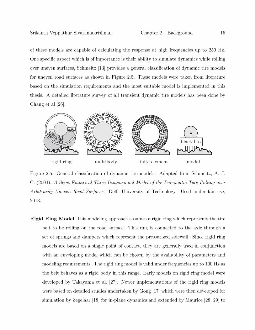
of these models are capable of calculating the response at high frequencies up to 250 Hz.
One specific aspect which is of importance is their ability to simulate dynamics while rolling
over uneven surfaces, Schmeitz [13] provides a general classification of dynamic tire models
for uneven road surfaces as shown in Figure 2.5. These models were taken from literature
based on the simulation requirements and the most suitable model is implemented in this
thesis. A detailed literature survey of all transient dynamic tire models has been done by
Chang et al [26].
Chapter 2
18
drum or on a flat road surface. The road experiments are carried out with instrumented
vehicles.
• Tyre type: In various publications, different types of tyres involving different
constructions are used: passenger car, (light) truck and aircraft tyres.
2.1.2 Literature review with regard to dynamic tyre models for rolling over uneven road
surfaces
In the literature, several tyre models are described that are developed to simulate the dynamic
response of a tyre when rolling over uneven road surfaces. These dynamic tyre models can
generally be classified in the following four model categories:
• Rigid ring models
• Multibody models
• Finite element models
• Modal models.
These model categories are illustrated in Figure 2.3.
rigid ring multibody finite element modal
black box
Figure 2.3: Different types of dynamic tyre models for uneven road surfaces.
Before the model categories are discussed in detail, it is useful to recapitulate the requirements
for tyre models for vehicle dynamic analyses as formulated in Chapter 1. These requirements
were that the tyre model should accurately predict the forces transmitted from the tyre to the
wheel spindle, the model should be practical in use (low computational effort, parameters
should be easily to obtain, etc.) and it should be widely applicable (ideally one model for all
Figure 2.5: General classification of dynamic tire models. Adapted from Schmeitz, A. J.
C. (2004). A Semi-Empirical Three-Dimensional Model of the Pneumatic Tyre Rolling over
Arbitrarily Uneven Road Surfaces. Delft University of Technology. Used under fair use,
2013.
Rigid Ring Model This modeling approach assumes a rigid ring which represents the tire
belt to be rolling on the road surface. This ring is connected to the axle through a
set of springs and dampers which represent the pressurized sidewall. Since rigid ring
models are based on a single point of contact, they are generally used in conjunction
with an enveloping model which can be chosen by the availability of parameters and
modeling requirements. The rigid ring model is valid under frequencies up to 100 Hz as
the belt behaves as a rigid body in this range. Early models on rigid ring model were
developed by Takayama et al. [27]. Newer implementations of the rigid ring models
were based on detailed studies undertaken by Gong [17] which were then developed for
simulation by Zegelaar [18] for in-plane dynamics and extended by Maurice [28, 29] to

Srikanth Veppathur Sivaramakrishnan Chapter 2. Background 16
account for out-of-plane dynamics. Other implementations of this model include the
work done by Allison and Sharp [30] and Bruni et al [31]. The rigid ring model has
been used for various commercial simulation tools for tires including MF-SWIFT by
TNO Automotive [32] and more recently, the UniTire model [33].
Multi-body Models In a multi-body simulation model, the tire belt is constructed as an
elaborate discrete point mass network which are interconnected through tension and
rotational springs. Multiple elastic belts with a similar discrete mass arrangement
are assumed to simulate lateral behavior which are again connected to each other
in a similar fashion. The elastic belts are connected to the axle through radial and
tangential springs. The tread elements are assumed to be brushes like that can slide
over or stick to the road surface. Eichler [34] introduced a three-dimensional version
of this model which was later commercially implemented as FTire [35, 36] and there
were studies on in-plane force transmissions which were conducted based on this model
by Dorfi [37]. Although these models are accurate, they tend to be computationally
heavy and difficult to parameterize.
Finite Element Models These models are constructed using detailed geometry and de-
scriptions of the tire. They are generally the most accurate in terms of simulation
output and can be directly used for simulating dynamic tire response. One of the ma-
jor drawbacks of this method is that they have the largest computational effort among
all models and are hence unsuitable for vehicle dynamic simulations. Finite element
models are generally used in conjunction with simpler discrete models as a virtual pro-
totyping tool to improve the speed of the simulations. Explicit finite element models
have been developed by Wu et al. [38] and Shobanie [39]. Some of the recent work on
finite element modeling which are usable in rigid ring tire models have been done by
Chae [40, 41]
Modal Models Generally, modal analysis is considered to be a ’black-box’ approach where
the relation between inputs (axle motion, road deflections) and outputs (spindle forces)

Srikanth Veppathur Sivaramakrishnan Chapter 2. Background 17
are identified using modal dynamics of the tire. One can either derive them through
FEA [22, 31] or through experimental modal analysis. One of the drawbacks with these
models is their linearity which fails to account for a lot of factors including the effect of
non-linear enveloping behavior, transient slip and the variations in longitudinal force
due to rolling velocity variations. Although they can be used up to frequencies of 250
Hz, they have greater applicability for noise and vibration analysis than for vehicle
dynamics.
2.3 Anti-lock Braking Systems
The two primary functions of a braking system are to retain control of the vehicle at a
steep inclination or a declination and to bring the vehicle to a complete stop in the shortest
distance possible. Conventionally, braking is accomplished in automobiles using a hydraulic
circuit. When the driver presses the brake pedal, it pushes fluid through the master cylinder
into the hydraulic circuit. This eventually translates into a pressure which would push the
brake shoes against the wheel and generate braking torque through friction.
Figure 2.6: Conventional vehicle braking system.

Srikanth Veppathur Sivaramakrishnan Chapter 2. Background 18
Initial systems were based on drum brakes on all four wheels where the drum is mounted on
the wheel with brake shoes positioned inside the drum. The hydraulic actuators press the
brake shoes against the drum and this would cause braking due to frictional force. Currently,
vehicles are equipped with disc brakes since they were more efficient during braking and had
a better heat dissipating mechanism. In this, a caliper is mounted on a wheel solid disc which
is attached to the wheel. The calipers are actuated through hydraulics and generate braking
force by clamping the disc through brake pads. A detailed diagram of a vehicle braking
system with disc brakes on the front and drum brakes on the rear is shown in Figure 2.6
Figure 2.7: Bendix ABS System Schematic.
Improvements in electronics led to the development of reliable control systems which could
be used for the improvement of safety systems. This led to the development of the Anti-lock
Braking System (ABS). This was a revolutionary concept in which the ABS controller cycles
the braking action such that the wheel is always at a desired optimum slip ratio and wheel
lock up is also prevented. As a result, this system retains directional control to the driver
even during severe braking events and prevents the vehicle from going unstable due to the
wheel slipping. Earlier versions of ABS began to appear in aircrafts as early as 1929 and they
Srikanth Veppathur Sivaramakrishnan Chapter 2. Background 19
remained exclusive due to their high costs. Modern ABS systems for use in automobiles were
introduced in 1971. The automotive industry was interested in utilizing this technology for
incorporating it as a safety system in their vehicles and began to adapt them for the consumer
level. Following their introduction in vehicles, ABS systems came to be widely adopted as
they drastically reduced the number of automotive-related accidents. Currently, ABS in a
vehicle is considered a critical safety system and is mandatory in many countries. Figure 2.7
shows a detailed overview of an ABS system. A time-line of the development of ABS systems
is described as an SAE Standard [42].
2.3.1 Principle of Operation
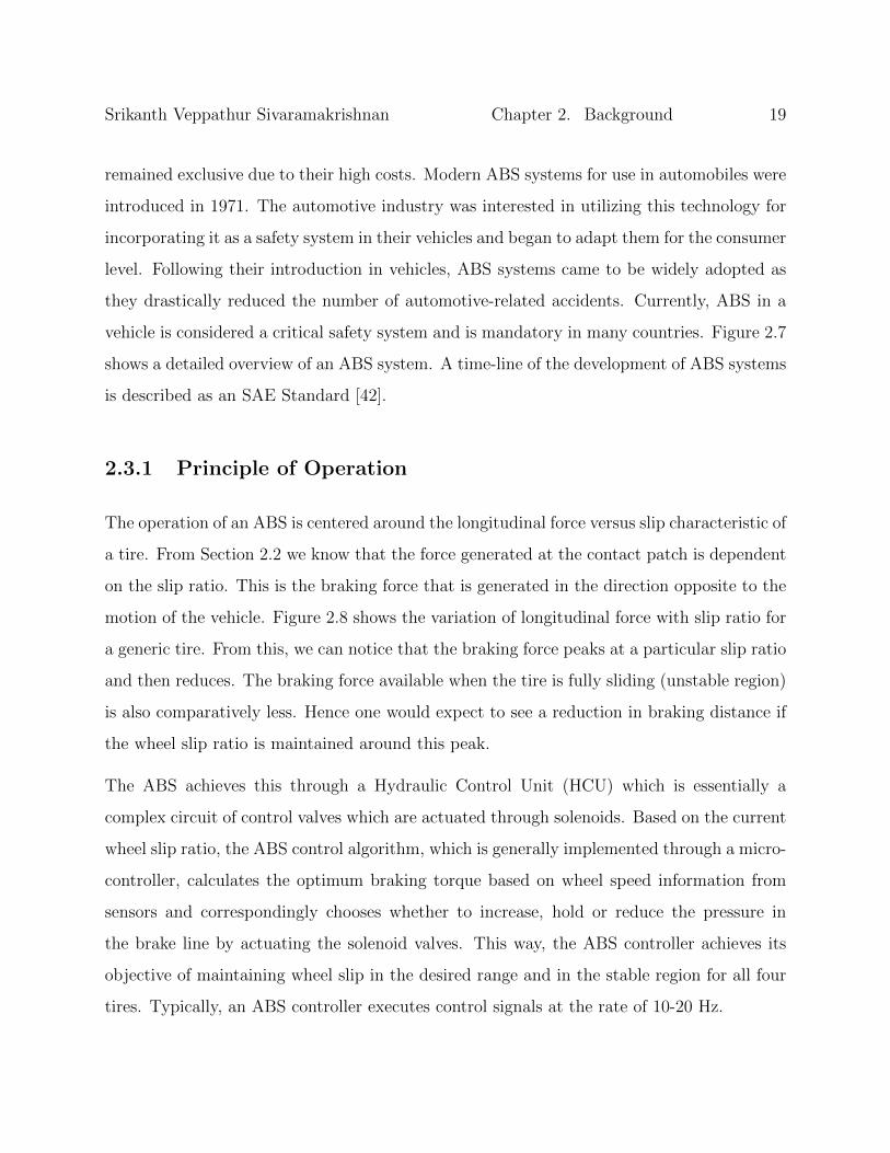
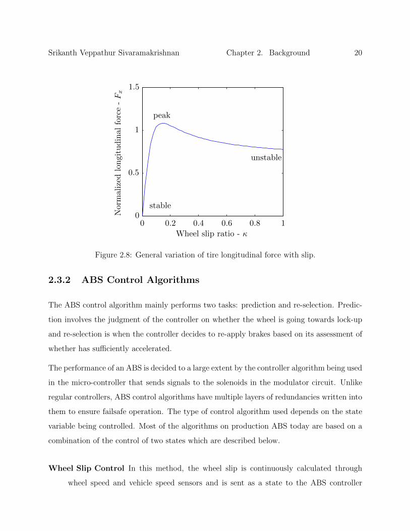
The operation of an ABS is centered around the longitudinal force versus slip characteristic of
a tire. From Section 2.2 we know that the force generated at the contact patch is dependent
on the slip ratio. This is the braking force that is generated in the direction opposite to the
motion of the vehicle. Figure 2.8 shows the variation of longitudinal force with slip ratio for
a generic tire. From this, we can notice that the braking force peaks at a particular slip ratio
and then reduces. The braking force available when the tire is fully sliding (unstable region)
is also comparatively less. Hence one would expect to see a reduction in braking distance if
the wheel slip ratio is maintained around this peak.
The ABS achieves this through a Hydraulic Control Unit (HCU) which is essentially a
complex circuit of control valves which are actuated through solenoids. Based on the current
wheel slip ratio, the ABS control algorithm, which is generally implemented through a micro-
controller, calculates the optimum braking torque based on wheel speed information from
sensors and correspondingly chooses whether to increase, hold or reduce the pressure in
the brake line by actuating the solenoid valves. This way, the ABS controller achieves its
objective of maintaining wheel slip in the desired range and in the stable region for all four
tires. Typically, an ABS controller executes control signals at the rate of 10-20 Hz.
Srikanth Veppathur Sivaramakrishnan Chapter 2. Background 20
Norm
alizedlongitudinalforce-Fx
Wheel slip ratio - κ
stable
peak
unstable
0 0.2 0.4 0.6 0.8 10
0.5
1
1.5
Figure 2.8: General variation of tire longitudinal force with slip.
2.3.2 ABS Control Algorithms
The ABS control algorithm mainly performs two tasks: prediction and re-selection. Predic-
tion involves the judgment of the controller on whether the wheel is going towards lock-up
and re-selection is when the controller decides to re-apply brakes based on its assessment of
whether has sufficiently accelerated.
The performance of an ABS is decided to a large extent by the controller algorithm being used
in the micro-controller that sends signals to the solenoids in the modulator circuit. Unlike
regular controllers, ABS control algorithms have multiple layers of redundancies written into
them to ensure failsafe operation. The type of control algorithm used depends on the state
variable being controlled. Most of the algorithms on production ABS today are based on a
combination of the control of two states which are described below.
Wheel Slip Control In this method, the wheel slip is continuously calculated through
wheel speed and vehicle speed sensors and is sent as a state to the ABS controller

Srikanth Veppathur Sivaramakrishnan Chapter 2. Background 21
which, based on various control methodologies drives the wheel slip to the desired
value. For wheel slip control, a model based law is adapted and currently this is the
most widely used method for advanced ABS systems used in modern automobiles. As
new control methodologies are formulated, various ABS algorithms have been proposed
and evaluated over the years towards creating a more robust system that would operate
under varying surface conditions. Slip control systems are known to work well for non-
decreasing force conditions.
Some of the earliest work done in this area includes the work done by Guntur [43, 44]
who proposed an adaptive brake control system. Taheri [45] investigated the use of non-
linear control laws for ABS and proposed a sliding mode based control algorithm [46],
a variation of which was also proposed by Drakunov et al [47]. Some authors including
Mauer [48] have proposed intelligent controllers based on fuzzy logic. Robust adaptive
control based on the Lyapunov method was suggested by Yu [49]. Due to the complex
nature of the hydraulic actuators which cause the pressure change in the brake line,
PID controllers are considered to be very robust and are popularly implemented at
the lower level, such as the ones proposed by Taheri and Law [50]. Recent advances
in sensor-based estimation techniques have led to the development of ABS control
methods based on intelligent tires as explained by Singh et al [51]. A comprehensive
review of various ABS wheel slip control algorithms has been explained by Aly [52].
Wheel Acceleration Control The concept of an ABS based on the measurement of pe-
ripheral angular acceleration of the wheel is implemented using a rule-based approach.
In this system, the braking cycle is designed to operate in three states: 1. Apply 2.
Hold 3. Release. The ABS controller is supplied with an exhaustive look-up table
that would account for different braking scenario. This table is essentially a set of
threshold values for wheel deceleration and slip ratios that would decide the brake
state during the prediction and re-selection stage. In a typical system, the ABS would
activate when the wheel deceleration drops below a specific value. The brake states
are continuously regulated such that the wheel deceleration and slip are within the

Srikanth Veppathur Sivaramakrishnan Chapter 2. Background 22
provided thresholds. This method is considered to be an indirect way of controlling
wheel slip because it requires careful adjustment of wheel acceleration thresholds to
achieve optimum performance.
Although more advanced controllers have been developed since their introduction,
wheel acceleration based ABS controllers are still popularly implemented in multi-
ple vehicle simulation models which require the inclusion of an ABS. One of the most
widely used algorithms in this regard is the Bosch R© HVE version 1 algorithm which has
been explained in detail by Roberts et al [53] and in their automotive handbook [54].
Ding et al [55, 56] implemented an improved version of this algorithm which was
originally designed for the 2002 Volkswagen R© Jetta with additional braking states
and self-adjusting thresholds and reference speeds. The Hardware-In-the-Loop (HIL)
validation [57] of this algorithm has also been explained in detail to demonstrate its
performance in comparison to a commercial ABS.
2.4 Previous Work on Dynamic Tire Models with ABS
Due to sustained interest from the industry to understand the influence of the dynamics of
tires and uneven roads on the performance of braking systems, various studies have been
undertaken using mutiple dynamic tire models. Earlier research by Zegelaar [58] involved
understanding the response of the rigid ring tire model to brake torque variations and their
experimental validation. Following this, Jansen et al [3] have focused on demonstrating the
potential of dynamic tire models such as the rigid ring model and their comparison with
steady-state and transient tire models for the analysis of the performance of ABS systems.
Following this, Paulwelussen et all [2] implemented the MF-SWIFT model in a full vehicle
with an ABS model and analyzed the braking response of their model at different velocities
under varying road conditions. Rangelov [59] constructed a simulink model of a quarter
car with MF-SWIFT and Bosch R© ABS algorithm and analyzed the performance of different

Srikanth Veppathur Sivaramakrishnan Chapter 2. Background 23
control methodologies. In addition to this, Adcox et al [60] developed a ring model with a
torsional spring and specifically analyzed the sensitivity of tire torsional dynamics on the
control effort of ABS and braking performance.
2.5 Conclusions
A review of literature of all the modeling aspects involved in this study has been conducted
in detail. Based on this, the following conclusions have been drawn:
• The reaction forces generated by a tire are influenced by vibrations induced in the belt
due to road unevenness, variations in brake torque and the oscillations in axle height.
The direct resultant of this is their effect on braking performance during the operation
of ABS.
• Simple transient models are not sufficient for modeling all the above influencing factors.
Various tire models are available to account for such factors.
• Dynamic tire models show considerable difference in response to braking in comparison
to steady-state and transient tire models which justify their necessity.
• The enveloping property of the tire should be included in conjunction with the tire
model to account for the filtering effect of the tire and the influence of road unevenness
on force response.
• Various detailed algorithms for ABS controllers are available in published literature
which can be adopted for analysis based on their closeness to commercial implementa-
tion.
• Requirements for vehicle models change according to their intended application (design
iterations, real-time testing, driving simulator etc.)

Srikanth Veppathur Sivaramakrishnan Chapter 2. Background 24
After carefully evaluating the advantages and drawbacks of various models described in the
literature, the following models have been chosen for implementation in the simulation tool
to be developed:
Tire Model For simulating the dynamics of the tire, the rigid ring model developed by
Zegelaar [1] is chosen because it is valid up to 100 Hz, accounts for the belt vibrations
and has potential for real-time implementation due to its speed.
Enveloping Model The semi-empirical tandem elliptical cam model, which was developed
by Schmeitz [13] has been selected due to its proven experimental validity and its
applicability to arbitrary uneven road profiles.
ABS Model For modeling the Anti-lock Braking System, an improved variation of the
Bosch R© ABS algorithm implemented by Ding [55] is chosen due to the availability of
source code and the algorithm has been validated to have accurately represented the
operation of a comparable commercial ABS system.
Vehicle Model The vehicle model would serve to integrate all the above developed sim-
ulation models as a single unit. It is proposed to implement a standalone version of
the simulation tool based on a quarter car vehicle model. Individual models also be
adapted to be implemented in advanced vehicle dynamic modeling software such as
CarSim R©.

Chapter 3
Mathematical Modeling
Following the detailed literature review and the consequent selection of available models from
available literature, the mathematical modeling of all components needs to be undertaken.
This chapter explains in detail the assumptions for each model, the equations and constitutive
relations that govern their behavior and their associated parameters. Detailed knowledge of
the mathematical aspects of the tire model, enveloping model and the ABS model will form
the basis for their implementation on a simulation platform. For the dynamic tire model,
most of the equations were based on the work by Zegelaar [1] and Schmeitz [13], which were
later improved by TNO Automotive during its commercial implementation as MF-SWIFT
and described in their equation manual [61].
3.1 Dynamic Tire Model
Developing the complete tire model involves two components: 1. Tire model and 2. En-
veloping model.
25

Srikanth Veppathur Sivaramakrishnan Chapter 3. Mathematical Modeling 26
3.1.1 Assumptions
Before beginning to derive the mathematical relations for the dynamics of the tire, important
assumptions need to be made to simplify the modeling process and remove unnecessary
factors that have low influence on the analysis task at hand. The major assumptions made
in this model are mentioned below:
• Only in-plane dynamics of the tire-wheel system is considered for modeling. Out-of-
plane motions and their related influence on force generation are neglected.
• The model is expected to be valid only up to 100 Hz where the rigid body modes are
dominant.
• The reaction forces generated at the wheel axle are calculated only along the longitu-
dinal and vertical direction (Fx and Fz respectively). Moments generated about the
lateral axis are calculated for rolling resistance and brake torque.
• The tire-wheel system is assumed to be rolling at an angular velocity of Ω at the start
of the simulation.
• Effect of tread element damping is neglected in the calculation of transient slip.
• Tire belt is assumed to be rigid and inextensible in its expected frequency range of
operation (<100 Hz).
• The elliptical cams used in the enveloping model are considered to be rigid and con-
strained to move only in the vertical direction.
• The tire is assumed to be symmetric about its axis of rotation. Loads and forces acting
on the tire are assumed to act along the Z-axis at the center of rotation.
• The influence of camber and toe are neglected
• Inflation pressure is assumed to be constant throughout the simulation.

Srikanth Veppathur Sivaramakrishnan Chapter 3. Mathematical Modeling 27
• The maximum height of the road disturbance is assumed to be less than 0.03 m.
3.1.2 Coordinate System
For all calculations, the right-handed cartesian coordinate system according to ISO 8855 is
used. For the X-axis, the forward direction is considered positive and is aligned along the
intersection of the wheel plane and the road plane. The Z-axis is chosen such that it is
aligned perpendicular to the road plane and the upwards direction is considered positive.
The Y -axis is chosen such that the axis system is right-handed. When the tire rolls in
the positive X direction, the angular velocity about the Y -axis is positive. Traction forces
are hence positive and the braking and rolling resistance forces are negative. The vertical
reaction force generated by the loaded tire is positive. Figure 3.1 shows the global coordinate
system as illustrated by Zegelaar [1].
Chapter 1
GmbH, Mercedes-Benz AG, PSA Peugeot-Citroën, Robert Bosch GmbH. Theobjectives of this research project are the development and implementation of amathematical model of a pneumatic tyre that is well suited for vehiclesimulations even under extreme manoeuvring conditions. The requirements forthe model development are:• A compact relatively fast tyre model, as it has to be used for vehicle dynamic
simulations.• Accurate representation of measured stationary slip characteristics.• High and low velocities, including starting to roll from stand-still.• Medium frequency range (f < 50 Hz).• Short wavelengths (λ > 0.2 m).• Uneven roads with relatively short and sharp unevennesses.In this thesis the development of the tyre model for in-plane dynamics will bediscussed, the model for the out-of-plane tyre dynamics is being developed byMaurice [65] while TNO is responsible for the professional software developmentof the model. The tyre in-plane dynamics refer to tyre vibrations in the wheelplane. The wheel plane is the central plane of the tyre normal to the axis ofrotation, see Figure 1.3. The tyre stands on the road plane and the contact patchis defined as the interface between tyre and road.
x
z
y
verticalwheel plane
road plane
lateral
longitudinal
Figure 1.3: The coordinate system used.
A right-handed Cartesian coordinate system (x,y,z) oriented according to ISO 8855is used. The x-axis is oriented along the intersection line of the wheel plane andthe road plane with the positive direction forwards. The z-axis is perpendicular tothe road plane with the positive direction upwards. The y-axis is perpendicular to
18
Figure 3.1: Global coordinate system. Adapted from Zegelaar, P. (1998). The dynamic
response of tyres to brake torque variations and road unevennesses. Delft University of
Technology. Used under fair use, 2013.
Srikanth Veppathur Sivaramakrishnan Chapter 3. Mathematical Modeling 28
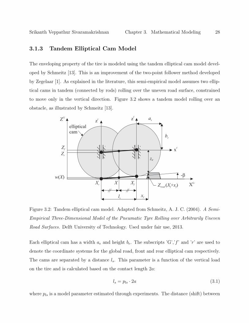
3.1.3 Tandem Elliptical Cam Model
The enveloping property of the tire is modeled using the tandem elliptical cam model devel-
oped by Schmeitz [13]. This is an improvement of the two-point follower method developed
by Zegelaar [1]. As explained in the literature, this semi-empirical model assumes two ellip-
tical cams in tandem (connected by rods) rolling over the uneven road surface, constrained
to move only in the vertical direction. Figure 3.2 shows a tandem model rolling over an
obstacle, as illustrated by Schmeitz [13].
The Quasi-Static Enveloping Behaviour of Pneumatic Tyres
115
x
zr
XG
xf
ze
xf
ZG
Z X xroad f f( + )
zf
X
ls
w X( )
XfXr
Zf
ae
be
-
Zr
ellipticalcam
Figure 4.18: The tandem model with elliptical cams.
The effective height (w) equals the height of the midpoint of the lower tandem rod. Thus, the
equation for the effective height reads:
( )2
f re
Z Zw X b
+= − (4.11)
where X is the global wheel centre longitudinal position and Zf and Zr are the global heights of
the front and rear ellipse centres, respectively. The inclination angle of the tandem rod
corresponds to the effective forward slope tan βy:
tan r fy
s
Z Z
lβ
−= (4.12)
For the front ellipse it will now be explained how the global height of the ellipse centre is
determined. The global height of the rear ellipse centre is obtained in the same way. As can be
seen in Figure 4.18, the front ellipse contacts the obstacle at the position where the road surface
height Zroad plus the distance ze (see equation (4.9)) is maximal. Consequently, the global
height of the ellipse centre can be obtained from the equation:
( ) ( )maxf road f f e fZ Z X x z x = + + (4.13)
In the simulation model, scans of the road height (Zroad) and ellipse height (ze) have to be taken
at a number of discrete positions (xf). Depending on the type of simulation, the size of the road
scan interval might be adjusted. For the simulations on obstacles, an interval of 1 mm was used
Figure 3.2: Tandem elliptical cam model. Adapted from Schmeitz, A. J. C. (2004). A Semi-
Empirical Three-Dimensional Model of the Pneumatic Tyre Rolling over Arbitrarily Uneven
Road Surfaces. Delft University of Technology. Used under fair use, 2013.
Each elliptical cam has a width ae and height be. The subscripts ’G’,’f ’ and ’r’ are used to
denote the coordinate systems for the global road, front and rear elliptical cam respectively.
The cams are separated by a distance ls. This parameter is a function of the vertical load
on the tire and is calculated based on the contact length 2a:
ls = pls · 2a (3.1)
where pls is a model parameter estimated through experiments. The distance (shift) between

Srikanth Veppathur Sivaramakrishnan Chapter 3. Mathematical Modeling 29
the cams increases as the load increases. The inputs to this model are the X and Z coordinates
of the actual road profile in the global frame of reference. This is transformed into an effective
plane height and slope which would serve as an input to the rigid ring tire model. The
effective plane height w is calculated for each road position X as the mid-point of the lower
tandem rod:
w(X) =Zf + Zr
2− be (3.2)
where Zf and Zr are the global heights of the front and rear cams respectively. The effective
plane slope β is calculated as:
β(X) = arctan
(Zr − Zf
ls
)(3.3)
For the front ellipse, we know its equation in the local coordinate system as:(xfae
)ce+
(zfbe
)ce= 1 (3.4)
where xf and zf are the local position coordinates for the front ellipse. The vertical distance
(ze) between the local X-axis and the ellipse for any local position xf is calculated based on
Equation (3.4) as:
ze(xf ) =
∣∣∣∣∣∣∣be ·(
1−( |xf |ae
)ce) 1
ce
∣∣∣∣∣∣∣ (3.5)
From Figure 3.2, we can observe the front ellipse rolling over an obstacle of height Zroad.
Thus the global height of the front ellipse(Zf ) is calculated using a maximal relation as the
sum of the road height and the vertical distance between the ellipse contact point and the
center:
Zf = max [Zroad(Xf + xf ) + ze(xf )] ∀ xf ∈ [−ae, ae] (3.6)
Equation (3.6) is a maximal relation because to calculate Zf it is necessary to find out where
the ellipse actually makes contact with the road profile. This is done using an iterative
procedure where the road profile is sampled at specific intervals around the global position
of the front ellipse Xf with a maximum limit of the ellipse width ae where the global height
of the front ellipse is calculated at each interval using Equation (3.6) and the maximum

Srikanth Veppathur Sivaramakrishnan Chapter 3. Mathematical Modeling 30
obtained value at the end of the iteration is taken as the final global height. The same
procedure is also repeated for the rear ellipse.
Special care must be given to the selection of the sample interval and the total scan width
because the number of points to scan at each road position would play a major role in de-
termining the speed and accuracy of the algorithm. Scan intervals which are too big might
lead to inaccurate results. Also, scanning the entire width of [−ae, ae] might severely slow
down the calculation speed as this step is repeated at each simulation time step. Generally,
the resolution of the road profile is taken as the sample interval and the scan width is ad-
justed accordingly to achieve the right balance between accuracy and speed. The maximum
allowable sampling interval is 2 cm to achieve acceptable results.
3.1.4 Rigid Ring Tire Model
This section details the modeling of the rigid ring dynamic tire model as explained by
Zegelaar [1] and adapted based on the current assumptions. This includes the calculations
for various properties of the tire including effective loading radius, forces in the contact patch
and related equations of motion.
In this model, the tire belt is modeled as a rigid ring connected to the axle or the rim through
springs and dampers which represent the pressurized sidewall. The ring is connected to the
road through a contact model which is represented as a transient slip model, as illustrated
in Figure 3.3. In this model, the translational sidewall stiffness and damping are represented
by cbx and kbx. cbθ and kbθ denote the rotational stiffness and damping. Vertical sidewall
stiffness and damping are represented by cbz and kbz respectively. Since the tire is assumed
to be symmetric, the stiffness and damping along the X and Z direction are assumed to be
the same.
Figure 3.4 shows deformations occurring in the tire ring of radius r. The tire-wheel system
is rotating at an undisturbed angular velocity Ω. The motion of the axle is represented by

Srikanth Veppathur Sivaramakrishnan Chapter 3. Mathematical Modeling 31
x
z
rigid tyre ring rim (axle)
slip model
road surface
155
cbkbx
cbx
cbz kbz
kb
Figure 3.3: Rigid ring tire model. Adapted from Zegelaar, P. (1998). The dynamic response
of tyres to brake torque variations and road unevennesses. Delft University of Technology.
Used under fair use, 2013.
xa and za. Consider a point O in the ring after a rotation of φ (φ = Ω). This point then
moves to A following the motion of the rim which is rotated by θa and translated by xa and
za. This then results in a deflection in the sidewall which results in the point moving to B
due to a rotation of θb and a translation of xb and zb in the ring.
Inputs and Outputs
The rigid ring model requires inputs from other models to simulate results, namely:
Axle Motion Axle motion is represented by xa, za, xa and za which are calculated from the
vehicle model. When the tire is loaded, the axle is given an initial vertical displacement
(which is negative) to represent the deflection in the tire. In the case of experiments
with a fixed axle, za is kept constant and za = 0.
Effective Road Profile This consists of the effective plane height w and plane angle β.
These values are calculated for each point in the road profile by the enveloping model.

Srikanth Veppathur Sivaramakrishnan Chapter 3. Mathematical Modeling 32
Development of the Rigid Ring Tyre Model
Chapter 4 the flexible ring model was considered, while in this chapter the rigidring model is developed. Secondly, here rim rotation results from twocontributions: the angle ϕ due to constant rotation and the small variation θa,while in Chapter 4 the total angle of rotation of the rim was represented by theangle ϕ. Thirdly, the variables vb and wb here denote the tangential and radialcomponents of the deformation of the tyre sidewalls, rather than the tangential
xxa xb
zb
za
z
B After additional
A After displacement
displacement and rotation of the tyre ring
and additional rotation of the rim
situationO Original undisturbed
Ω
O
A B
ϕ
θa
θb
r
The tangential vb and radial wb components of the deformation of the tyresidewall are equal to the difference between the positions of points A and B:
vw
rx xz zb
b
a a
a a
b a
b a
b a
=+ − ++ +
−−−
cos sinsin cos
ϕ θ ϕ θϕ θ ϕ θ
θ θ
0
(7.1)
Or:
v x xb b a= −Q (7.2)
where Q denotes the transformation matrix from the fixed to the rotatingcoordinate system and the deformations and positions are written as:
v v w x x z x x zb b bT
a a a aT
b b b bT= = =, ,θ θ (7.3)
The time rate of change of the tyre sidewall deformation reads:
157
Figure 3.4: Deformations in the tire. Adapted from Zegelaar, P. (1998). The dynamic
response of tyres to brake torque variations and road unevennesses. Delft University of
Technology. Used under fair use, 2013.
Braking Moment This is denoted by May and this input is provided by the braking module
which calculates the applied torque at the axle during a braking event. This can either
be due to ABS or manual braking.
Based on the above inputs, the rigid ring model calculates the following outputs which serve
as inputs to the vehicle and the braking model:
Reaction Forces These are the forces acting on the vehicle from the tire, denoted by Fbx
and Fbz and are from the equations of motion for the ring model.
Wheel Slip The dynamics of the tire rolling over uneven surfaces causes fluctuations in
the angular velocity of the wheel due to the deformation of the belt in the rotational
direction. The practical slip ratio κ, which acts an input to the braking module is
calculated from the theoretical slip in the contact patch ζcx along the longitudinal
direction.
Contact Patch Length This is calculated either based on the load acting on the contact
patch or the vertical deflection of the tire. The length of the contact patch is denoted
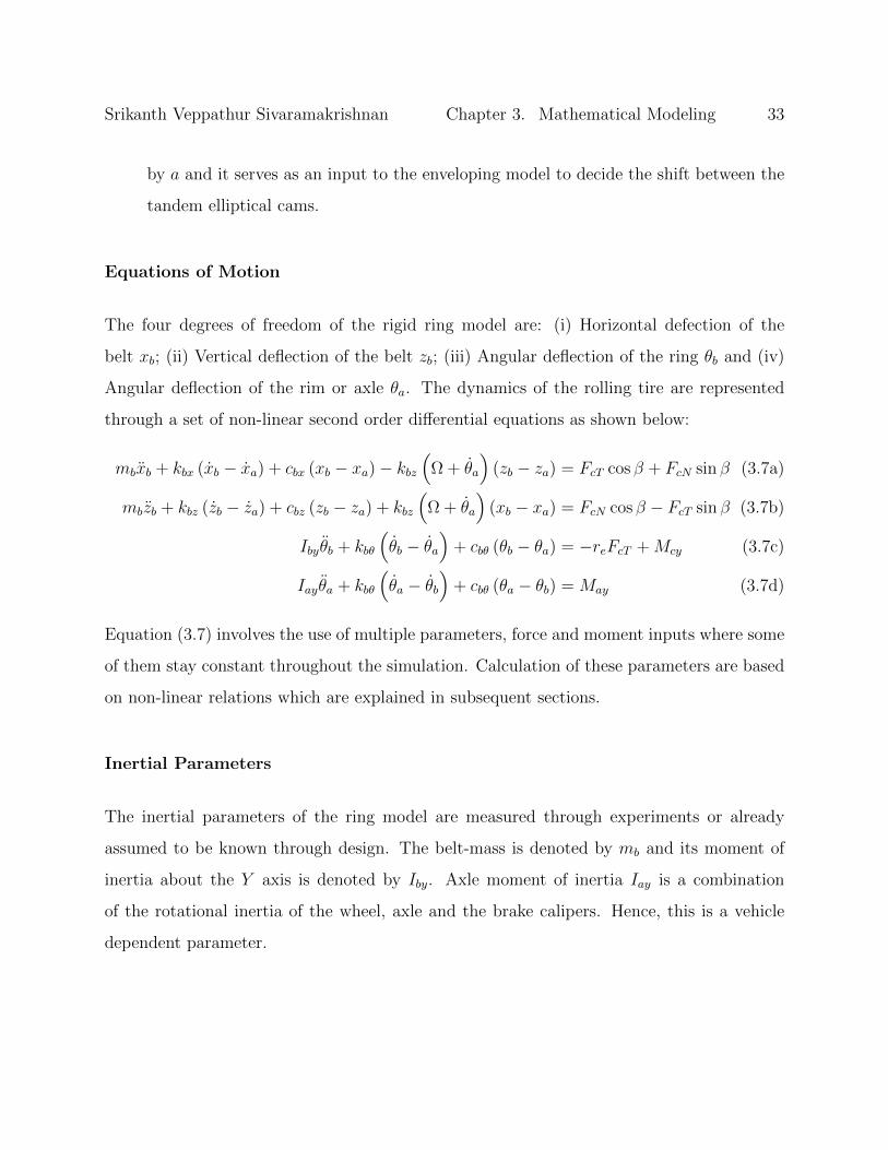
Srikanth Veppathur Sivaramakrishnan Chapter 3. Mathematical Modeling 33
by a and it serves as an input to the enveloping model to decide the shift between the
tandem elliptical cams.
Equations of Motion
The four degrees of freedom of the rigid ring model are: (i) Horizontal defection of the
belt xb; (ii) Vertical deflection of the belt zb; (iii) Angular deflection of the ring θb and (iv)
Angular deflection of the rim or axle θa. The dynamics of the rolling tire are represented
through a set of non-linear second order differential equations as shown below:
mbxb + kbx (xb − xa) + cbx (xb − xa)− kbz(
Ω + θa
)(zb − za) = FcT cos β + FcN sin β (3.7a)
mbzb + kbz (zb − za) + cbz (zb − za) + kbz
(Ω + θa
)(xb − xa) = FcN cos β − FcT sin β (3.7b)
Ibyθb + kbθ
(θb − θa
)+ cbθ (θb − θa) = −reFcT +Mcy (3.7c)
Iayθa + kbθ
(θa − θb
)+ cbθ (θa − θb) = May (3.7d)
Equation (3.7) involves the use of multiple parameters, force and moment inputs where some
of them stay constant throughout the simulation. Calculation of these parameters are based
on non-linear relations which are explained in subsequent sections.
Inertial Parameters
The inertial parameters of the ring model are measured through experiments or already
assumed to be known through design. The belt-mass is denoted by mb and its moment of
inertia about the Y axis is denoted by Iby. Axle moment of inertia Iay is a combination
of the rotational inertia of the wheel, axle and the brake calipers. Hence, this is a vehicle
dependent parameter.

Srikanth Veppathur Sivaramakrishnan Chapter 3. Mathematical Modeling 34
Sidewall Stiffness and Damping
The vertical and rotational stiffness and damping of the sidewall are calculated from the
natural frequencies of the in-plane rigid body modes of the unloaded, inflated tire which is
mounted on a fixed spindle without touching the ground. Sidewall stiffness and damping
values are calculated as:
cbx0 = cbz0 = 4π2 ·mb · f 2long (3.8a)
cbθ0 = 4π2 · Iby · f 2windup (3.8b)
kbx0 = kbz0 = 4π · ζlong ·mb · flong (3.8c)
kbθ0 = 4π · ζwindup · Iby · fwindup (3.8d)
where flong is the primary eigen-frequency (in Hz) and ζlong is the dimensionless damping
factor of the vertical/longitudinal motion of the belt, also known as the in-plane vertical
mode. fwindup and ζwindup are correspondingly the eigen-frequency and damping factor of
the rotational motion of the belt, also known as the in-plane torsional mode. The subscript
’0’ denotes stiffness and damping values of the tire at non-rolling conditions. Equation (3.8)
is valid only for rigid body modes because under such situations, the belt moves as a rigid
body and can be approximated to have the same behavior as a single degree of freedom
mass, spring and damper. During the modal analysis, the spindle is clamped to ensure the
belt mass is the primary inertial component.
Based on previous studies by Vinesse [62] and Zegelaar [58], it is understood that the natural
frequencies of the rolling tire change with velocity. Hence, the actual sidewall stiffness is much
lower than the values obtained from the natural frequencies at stationary condition using
Equation (3.8). In order to account for this effect, the sidewall stiffness is made dependent

Srikanth Veppathur Sivaramakrishnan Chapter 3. Mathematical Modeling 35
on the rolling velocity, pressure and load through correction factors:
cbx = cbx0 (1 + 0.65 · dpi)(
1− qbV x√QV
)(3.9a)
cbz = cbz0 (1 + 0.65 · dpi)(
1− qbV z√QV
)(3.9b)
cbθ = cbθ0 (1 + 0.49 · dpi)(
1− qbV θ√QV
)(3.9c)
where the variable QV is a non-dimensional quantity which represents the rate of deformation
of the tire due to rolling, calculated using the relation:
QV =
∣∣∣Ω + θa
∣∣∣V0
√(xb − xa)2 + (zb − za)2 (3.10)
where V0 is the nominal rolling velocity in m/s. The pressure dependency of sidewall stiffness
is included using empirical factors. The variable dpi measures the change in inflation pressure:
dpi =P − P0
P0
(3.11)
where P0 is the nominal inflation pressure and P is the current inflation pressure, measured
either in bar or kPa.
Normal Force in the Contact Patch
The normal force in the contact patch is represented by FcN which is a product of the residual
stiffness and the residual deflection in the contact patch. This occurs due to the fact that
the total deformation of the tire is larger than the displacement of the rigid ring. The total
vertical stiffness is hence a combination of the sidewall stiffness cbz and the residual stiffness.
The normal force in the contact patch has a non-linear relation with the residual deflection
and is represented as a third order polynomial:
FcN =
qFzr3ρ3zr + qFzr2ρ
2zr + qFzr1ρzr if ρzr > 0
0 if ρzr ≤ 0
(3.12)
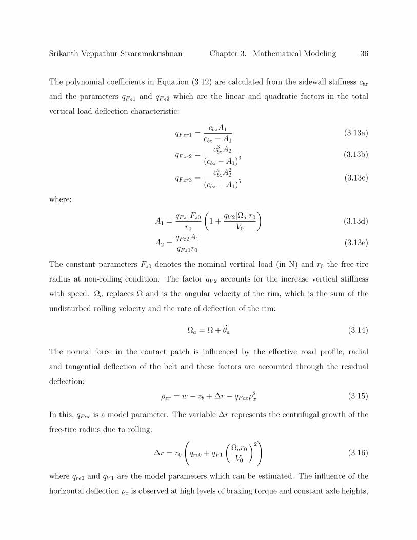
Srikanth Veppathur Sivaramakrishnan Chapter 3. Mathematical Modeling 36
The polynomial coefficients in Equation (3.12) are calculated from the sidewall stiffness cbz
and the parameters qFz1 and qFz2 which are the linear and quadratic factors in the total
vertical load-deflection characteristic:
qFzr1 =cbzA1
cbz − A1
(3.13a)
qFzr2 =c3bzA2
(cbz − A1)3 (3.13b)
qFzr3 =c4bzA
22
(cbz − A1)5 (3.13c)
where:
A1 =qFz1Fz0r0
(1 +
qV 2|Ωa|r0
V0
)(3.13d)
A2 =qFz2A1
qFz1r0
(3.13e)
The constant parameters Fz0 denotes the nominal vertical load (in N) and r0 the free-tire
radius at non-rolling condition. The factor qV 2 accounts for the increase vertical stiffness
with speed. Ωa replaces Ω and is the angular velocity of the rim, which is the sum of the
undisturbed rolling velocity and the rate of deflection of the rim:
Ωa = Ω + θa (3.14)
The normal force in the contact patch is influenced by the effective road profile, radial
and tangential deflection of the belt and these factors are accounted through the residual
deflection:
ρzr = w − zb + ∆r − qFcxρ2x (3.15)
In this, qFcx is a model parameter. The variable ∆r represents the centrifugal growth of the
free-tire radius due to rolling:
∆r = r0
(qre0 + qV 1
(Ωar0
V0
)2)
(3.16)
where qre0 and qV 1 are the model parameters which can be estimated. The influence of the
horizontal deflection ρx is observed at high levels of braking torque and constant axle heights,

Srikanth Veppathur Sivaramakrishnan Chapter 3. Mathematical Modeling 37
Vc,sxCκVcr
ccx
in the measurements. The horizontal mode is the mode of the model with thehighest natural frequency (100-140 Hz) and it has very small damping at lowvelocities. The relative damping of this mode increases by the introduction of thetread element damping. The resulting larger relative damping has two positiveeffects: first, the unwanted vibrations of the mode are damped rather quickly;and second, the larger damping puts less restrictions to the step size of thenumerical integration process.
Rolling resistance
The rolling resistance is modelled as an external torque Mcy acting from the roadon the tyre ring:
M r f Fcy e r cN b= − ⋅ +sgn Ω θ (7.32)
where fr denotes the rolling resistance coefficient. If the rotational tyre ringvelocity changes sign, the rolling resistance torque changes sign as well. Close to
169
____
(a) Tread element model.
Vc,sx
Ω
Vx
re
rim
tire
road surface
S(a) kinematics of a rolling tyre
(b) Brush-type tread elements.
Figure 3.5: Tire-road contact model. Adapted from Zegelaar, P. (1998). The dynamic
response of tyres to brake torque variations and road unevennesses. Delft University of
Technology. Used under fair use, 2013.
which is calculated as:
ρx = (xb − xa) + r0(θb − θa) (3.17)
Tire-Road Contact Model
The tangential force acting in the contact patch is represented by FcT . This force is generated
due to slip ζcx occurring in the contact patch. The dynamic interactions between the tread
elements of the rolling tire and the ground leads to variations in the slip. The slip is also
influenced by the deformation of the belt and variations in the effective rolling radius. This
plays a crucial role in the analysis of ABS systems.
Hence, a contact model is required for the tread elements to simulate the transient slip. This
is accomplished using an analytical model, as shown in Figure 3.5(a) where the non-steady
state slip variations are modeled using a first-order approximation which is based on the
relaxation length σcx and slip velocities calculated from belt deflections:
σc · ζcx + |Vcr| = −Vc,sx (3.18)
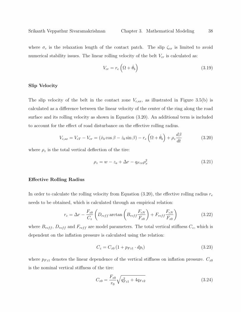
Srikanth Veppathur Sivaramakrishnan Chapter 3. Mathematical Modeling 38
where σc is the relaxation length of the contact patch. The slip ζcx is limited to avoid
numerical stability issues. The linear rolling velocity of the belt Vcr is calculated as:
Vcr = re
(Ω + θb
)(3.19)
Slip Velocity
The slip velocity of the belt in the contact zone Vc,sx, as illustrated in Figure 3.5(b) is
calculated as a difference between the linear velocity of the center of the ring along the road
surface and its rolling velocity as shown in Equation (3.20). An additional term is included
to account for the effect of road disturbance on the effective rolling radius.
Vc,sx = VcT − Vcr = (xb cos β − zb sin β)− re(
Ω + θb
)+ ρz
dβ
dt(3.20)
where ρz is the total vertical deflection of the tire:
ρz = w − za + ∆r − qFcxρ2x (3.21)
Effective Rolling Radius
In order to calculate the rolling velocity from Equation (3.20), the effective rolling radius re
needs to be obtained, which is calculated through an empirical relation:
re = ∆r − Fz0Cz
(Dreff arctan
(Breff
FcNFz0
)+ Freff
FcNFz0
)(3.22)
where Breff , Dreff and Freff are model parameters. The total vertical stiffness Cz, which is
dependent on the inflation pressure is calculated using the relation:
Cz = Cz0 (1 + pFz1 · dpi) (3.23)
where pFz1 denotes the linear dependence of the vertical stiffness on inflation pressure. Cz0
is the nominal vertical stiffness of the tire:
Cz0 =Fz0r0
√q2Fz1 + 4qFz2 (3.24)
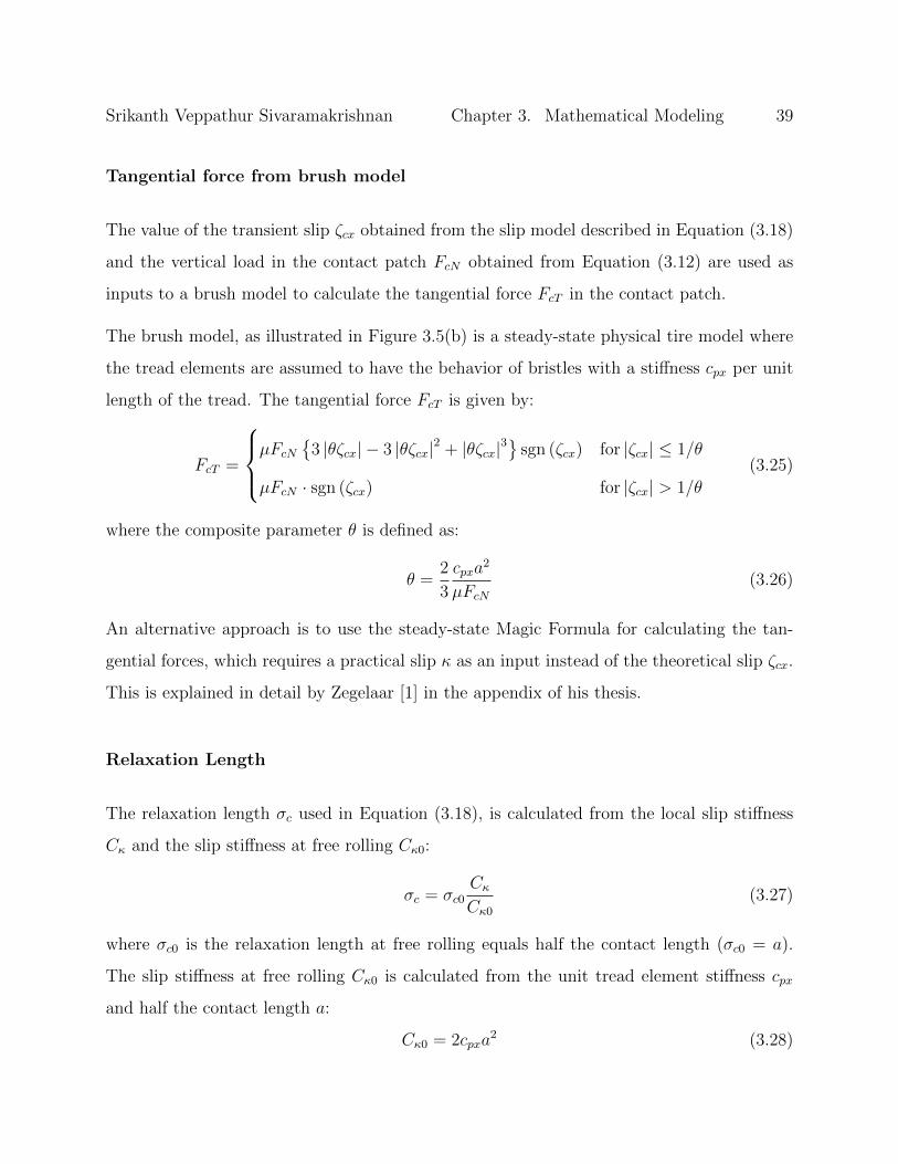
Srikanth Veppathur Sivaramakrishnan Chapter 3. Mathematical Modeling 39
Tangential force from brush model
The value of the transient slip ζcx obtained from the slip model described in Equation (3.18)
and the vertical load in the contact patch FcN obtained from Equation (3.12) are used as
inputs to a brush model to calculate the tangential force FcT in the contact patch.
The brush model, as illustrated in Figure 3.5(b) is a steady-state physical tire model where
the tread elements are assumed to have the behavior of bristles with a stiffness cpx per unit
length of the tread. The tangential force FcT is given by:
FcT =
µFcN
3 |θζcx| − 3 |θζcx|2 + |θζcx|3
sgn (ζcx) for |ζcx| ≤ 1/θ
µFcN · sgn (ζcx) for |ζcx| > 1/θ
(3.25)
where the composite parameter θ is defined as:
θ =2
3
cpxa2
µFcN(3.26)
An alternative approach is to use the steady-state Magic Formula for calculating the tan-
gential forces, which requires a practical slip κ as an input instead of the theoretical slip ζcx.
This is explained in detail by Zegelaar [1] in the appendix of his thesis.
Relaxation Length
The relaxation length σc used in Equation (3.18), is calculated from the local slip stiffness
Cκ and the slip stiffness at free rolling Cκ0:
σc = σc0CκCκ0
(3.27)
where σc0 is the relaxation length at free rolling equals half the contact length (σc0 = a).
The slip stiffness at free rolling Cκ0 is calculated from the unit tread element stiffness cpx
and half the contact length a:
Cκ0 = 2cpxa2 (3.28)
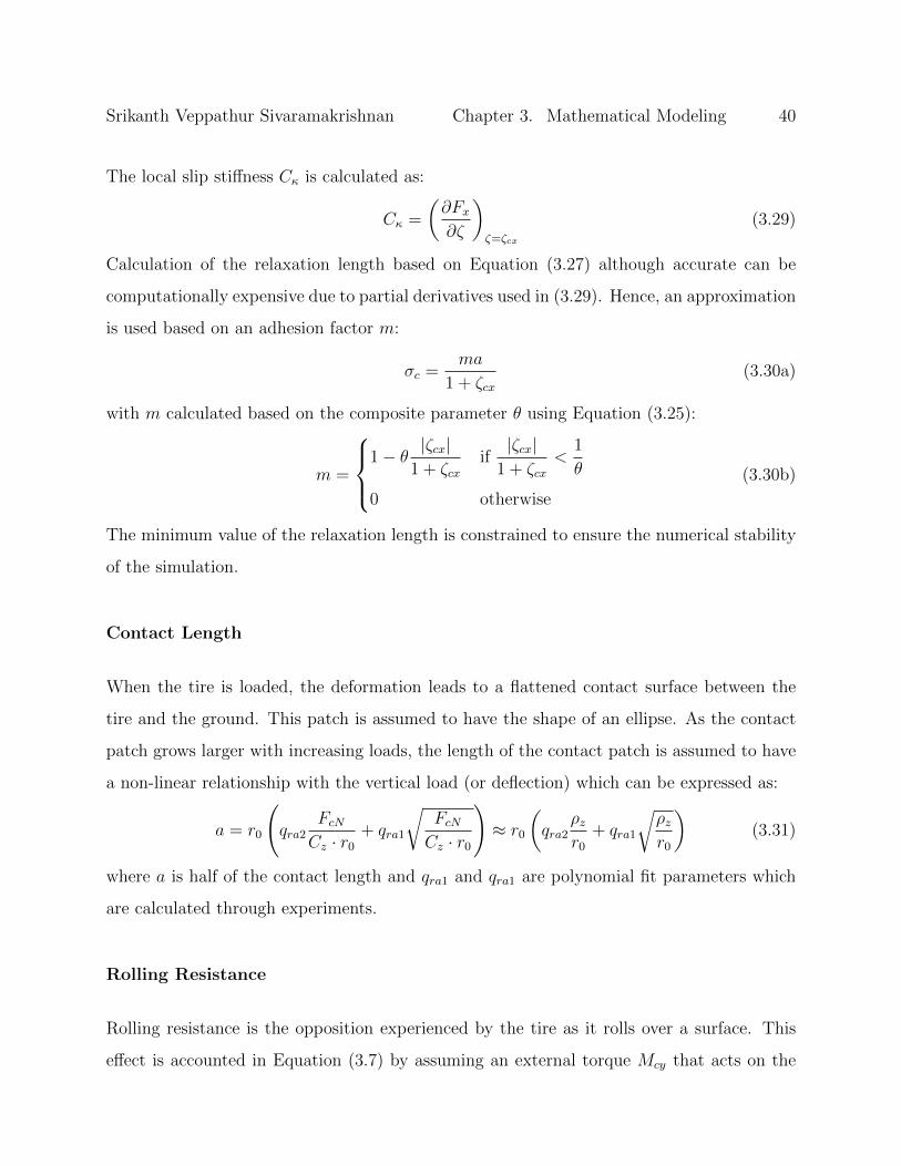
Srikanth Veppathur Sivaramakrishnan Chapter 3. Mathematical Modeling 40
The local slip stiffness Cκ is calculated as:
Cκ =
(∂Fx∂ζ
)ζ=ζcx
(3.29)
Calculation of the relaxation length based on Equation (3.27) although accurate can be
computationally expensive due to partial derivatives used in (3.29). Hence, an approximation
is used based on an adhesion factor m:
σc =ma
1 + ζcx(3.30a)
with m calculated based on the composite parameter θ using Equation (3.25):
m =
1− θ |ζcx|
1 + ζcxif|ζcx|
1 + ζcx<
1
θ
0 otherwise
(3.30b)
The minimum value of the relaxation length is constrained to ensure the numerical stability
of the simulation.
Contact Length
When the tire is loaded, the deformation leads to a flattened contact surface between the
tire and the ground. This patch is assumed to have the shape of an ellipse. As the contact
patch grows larger with increasing loads, the length of the contact patch is assumed to have
a non-linear relationship with the vertical load (or deflection) which can be expressed as:
a = r0
(qra2
FcNCz · r0
+ qra1
√FcNCz · r0
)≈ r0
(qra2
ρzr0
+ qra1
√ρzr0
)(3.31)
where a is half of the contact length and qra1 and qra1 are polynomial fit parameters which
are calculated through experiments.
Rolling Resistance
Rolling resistance is the opposition experienced by the tire as it rolls over a surface. This
effect is accounted in Equation (3.7) by assuming an external torque Mcy that acts on the
Srikanth Veppathur Sivaramakrishnan Chapter 3. Mathematical Modeling 41
ring:
Mcy = −refrFcN · sgn(
Ω + θb
)(3.32)
where fr is the rolling resistance coefficient. This coefficient is assumed to vary as a non-linear
polynomial function of speed and is expressed as:
fr =
(qsy1 + qsy3
∣∣∣∣VxV0
∣∣∣∣+ qsy4
(VxV0
)4)(
P
P0
)qsy8(3.33)
Forces at the Axle
The forces generated by the tire at the axle serve as the outputs from the tire model to the
vehicle model. They are calculated from the belt forces based on Equation (3.7) as:
Fxt = cbx (xb − xa) + kbx (xb − xa)− kbx(
Ω + θa
)(zb − za) (3.34a)
Fzt = cbz (zb − za) + kbz (zb − za) + kbz
(Ω + θa
)(xb − xa) (3.34b)
3.2 Anti-lock Braking System Model
An ABS model consists of two main components: 1. Control algorithm and 2. Pressure
model. Both these components are very essential to produce accurate results because having
an advanced control algorithm with a simplistic pressure model can lead to un-realistic
results. Also, having a detailed pressure model without a robust algorithm can also lead
to unfavorable results. Hence, a balance needs to be maintained to ensure confidence in
simulation results.
3.2.1 Inputs and Outputs
Since the ABS unit is only responsible for braking control, the system has a limited set of
inputs and outputs:

Srikanth Veppathur Sivaramakrishnan Chapter 3. Mathematical Modeling 42
Inputs : The ABS unit requires longitudinal slip κ and the wheel acceleration ε from the
tire model.
Outputs : Based on the inputs, the ABS with the included pressure model calculates the
braking torque May which is again sent to the tire model.
3.2.2 Assumptions
The hydraulic circuit of a braking system is an extremely complex system. A number of
assumptions were made which were aimed towards simplifying the modeling process and on
removing factors that had low influence on ABS performance:
• The ABS controller is assumed to know wheel slip and vehicle speed information
through sensors.
• Pressure in the master cylinder is assumed to be a constant value.
• Braking torque at the axle is considered to be linearly proportional to the pressure in
the brake line.
• Wheel slip and acceleration thresholds do not change during the simulation.
• The delay in the valves is represented as a first order delay.
• Mechanical delay in converting the pressure in the brake line to torque is taken to be
a constant value in time.
• The rate of increase and decrease of pressure during different brake states remain
constant and cannot be changed during the simulation.
• A minimum speed is required for the operation of the ABS system below which the
braking module switches to manual braking.

Srikanth Veppathur Sivaramakrishnan Chapter 3. Mathematical Modeling 43
3.2.3 Brake States
The operating algorithm of an ABS is characterized by the number and the type of brake
states utilized by the ABS to achieve optimal control of slip and wheel acceleration. The
ABS control logic, as designed by Ding et al [55] has the following primary states for the
braking system:
Initialize The ABS begins in this state where the output pressure in the wheel cylinder is
set to the master cylinder pressure. This is done to ensure proper build up of pressure
before regulation.
Hold Brake Pressure In this state, the ABS directs the wheel cylinder pressure to be
maintained in the previous control cycle. This is generally used when the slip and
wheel acceleration fall in the desired range.
Increase Brake Pressure In this, the brake pressure in the wheel cylinder is set to increase
from its current level up to the master cylinder pressure at a normal rate. The behavior
of the wheel cylinder is modeled according to Equation (3.35).
Fast Increase Brake Pressure The wheel cylinder pressure is regulated to increase at
a faster rate than the normal rate. This is generally done in cases where a sudden
increase in braking force is required (changing surface conditions etc.).
Decrease Brake Pressure This is also known as the pressure release state where the brake
pressure in the wheel cylinder is set to decrease from its current to atmospheric pressure.
The behavior of the wheel cylinder is modeled according to Equation (3.36).
Step Increase Brake Pressure This is a hybrid-state in which two operations are done
in a cycle: 1. Increase 2. Hold. This was introduced to increase the brake pressure and
also maintain the wheel acceleration without waiting for the controller to re-calculate
until the next cycle. Apart from the regular thresholds in the controller, this stage has

Srikanth Veppathur Sivaramakrishnan Chapter 3. Mathematical Modeling 44
a separate wheel acceleration threshold where the pressure is set to hold for a specific
amount of time when exceeded.
Step Decrease Brake Pressure The operation of this state is based on the same principle
as the step increase in brake pressure with the only difference being in this case the
brake pressure is decreased in cycles of decrease and hold (for a specified time).
Exit Braking This state is used when the vehicle is below a minimum speed where the
ABS shuts off and switches to manual braking.
3.2.4 ABS Control Cycling
An ABS system deployed in a vehicle is designed to control four wheels with a single con-
troller. In a general scenario, it might be too difficult to calculate control signals all four
wheels in a single cycle. This is accomplished by the use of controller flags where one wheel
is controlled during a cycle and this is rotated after each cycle. This way, all four wheels are
controlled at a reasonable rate. This method is illustrated in Figure 3.6.
3.2.5 State Selection Rules
The selection of brake states are made using a state-flow based approach where the decisions
are made based on a set of rules and thresholds. Figure 3.7 shows the chart used in this
system for the selection of states. Here, κ denotes the wheel slip and ε denotes the peripheral
acceleration of the wheel. This was previously designed at the Intelligent Transportation
Laboratory with a fixed set of thresholds which are being used.

Srikanth Veppathur Sivaramakrishnan Chapter 3. Mathematical Modeling 45
Release Rear-LeftSet
Flag RL = 0Count = 0
Control Rear-LeftSet
Flag RL = 0
IdleSet
Count = Count +1
Control Rear-RightSet
Flag RR = 0
Release Rear-RightSet
Flag RR = 0Count = 0
Is Count = 0 and Brake Pedal =1
?
IdleSet
Count = Count +1 True
Control Front-LeftSet
Flag FL = 0
Release Front-LeftSet
Flag FL = 0Count = 0
IdleSet
Count = Count +1
IsCount > 3
?
True
Release Front-RightSet
Flag FR = 0Count = 0
IdleSet
Count = Count +1
Start ABS Braking
IsBrake Pedal = 1
?
True
IsCount > 3
?
True
IsCount > 3
?
True
IsCount > 3
?
IsCount > 3
?
True
True
False
Exit ABS Braking
False
Figure 3.6: ABS control cycling between different tires.

Srikanth Veppathur Sivaramakrishnan Chapter 3. Mathematical Modeling 46
StartIs
Flag = 1 and Vx > 4 and κ > 0.08 ?
Isκ > 0.14
?
Decrease Brake Pressure
True
True
HoldBrake Pressure
False
Isκ > 0.14
and Flag = 1 ?
True
IsVx < minimum
speed ?
False
ReleaseBrakePressure
True
IsVx < minimum
speed ?True
Isκ < 0.135
and Flag = 1 ?
Hold BrakePressure
Count = Count + 1
Isκ > 0.08 ?
Slow IncreaseBrakePressure
Set Count = 0
Is( κ < 0.12
and Vx < 10 )or Count > 640 ?
Isκ > 0.15
?
True
True True
IsVx < minimum
speed ?Is
( κ < 0.135or Vx < 1 )or Flag = 1 ?
True
FalseTrue
False
True
False
Exit ABS Braking
Fast IncreaseBrakePressure
Count = Count + 1
Ism1f.ε> 15m1 ?
m1 = m1f.ε/15
True
Count = 0m1 = m1f.ε/15
Isε > 2 and Flag = 1
?
True
Isε > 5 or Count > 240
?
True
False
Figure 3.7: Flowchart for the selection of brake states.
Srikanth Veppathur Sivaramakrishnan Chapter 3. Mathematical Modeling 47
3.2.6 Pressure Model
In an ABS system, the brake pressure is regulated by means of electromagnetic valves that
are installed in the Hydraulic Control Unit (HCU). The pressure can be regulated through
three states: 1. Pressure increase; 2. Pressure hold; and 3. Pressure release.
In the pressure increase mode, the wheel cylinder pressure Pw is assumed to have an expo-
nential increase and is calculated as:
Pw(t) = Pm −[(Pm − Pw0)φinc −Kincφinc(t− t0)
]1/φinc
(3.35)
where Pw0 is the wheel cylinder pressure at the previous simulation time-step t0. Pm is
the pressure at the master cylinder. Kinc and φinc are model parameters for the response
characteristics of the brake system.
In the pressure release mode, the pressure in the brake cylinder pressure is governed by the
following expression:
Pw(t) =[(Pw0 − Pa)φdec −Kdecφdec(t− t0)
]1/φinc
+ Pa (3.36)
where Pa is the atmospheric pressure. The parameters Kdec and φdec are selected based on
the desired behavior for pressure decrease. The pressure in the wheel cylinder is retained in
its previous value during the hold phase.
The pressure in the wheel cylinder Pw is then converted into brake torque May using the
relation:
May = Pw · Cp (3.37)
where Cp is the brake torque gain (N.m/Pa) and this value is different for the front wheels
and rear wheels . The brake torque is applied to the tire model after a first-order transport
delay to account for the dynamics of the valve.

Srikanth Veppathur Sivaramakrishnan Chapter 3. Mathematical Modeling 48
3.3 Quarter Car Model
The quarter car model is the most commonly used for ride analysis and braking studies. The
model considered here is assumed to have suspensions in both X and Z directions. Inputs
to this model constitute reaction forces from the dynamic tire model to the axle. Desired
outputs are the axle motions that serve as inputs to the tire model. The quarter car model
is illustrated as shown in Figure 3.8.
Tire
Sprung Mass
Axle
zs
xs
zaxa
ma
ms
Csx
Ksx
Csz Ksz
Figure 3.8: Quarter car model.
The equations of motion of the quarter car model are calculated as:
ma · xa +Ksx (xa − xs) + Csx (xa − xs) = Fxt (3.38a)
ms · xs +Ksx (xs − xa) + Csx (xs − xa) = 0 (3.38b)
ma · za +Ksz (za − zs) + Csz (za − zs) = Fzt +mag (3.38c)
ms · zs +Ksz (zs − za) + Csz (zs − za) = msg (3.38d)
where Csx, Csz, Ksx and Ksz are the suspension stiffness and damping values along the X
and Z directions respectively. ms is the vehicle sprung mass and ma is the unsprung mass

Srikanth Veppathur Sivaramakrishnan Chapter 3. Mathematical Modeling 49
which consists of the mass of the axle including the suspension and braking elements. Since
the tire is modeled as a separate rigid ring element, their inertial properties are not added to
the axle mass. Here, the assumptions are that the stiffness and damping elements are linear
and the deflection along the X axis and Z axis are independent of each other.
3.4 Conclusions
Detailed mathematical models of all the subsystems of the simulation tool, including the
dynamic tire model, ABS model and the vehicle model were developed. This was done by
deciding on a set of assumptions for simplifying the model and the equations were derived
based on the literature. These models were then used to develop a simulation platform and
integrated to optimize performance as discussed in subsequent chapters.

Chapter 4
Implementation
Following the derivation of equations for the models, it was necessary to develop their models
in a platform that can conduct the simulations and can be used to analyze the results. This
chapter describes the methodology adopted towards the selection of simulation platform,
development of models and the requirements for the exchange of experimental and parameter
data.
4.1 Design Requirements
Based on the objectives of the model defined in Section 1.2.1, the following design require-
ments are outlined that are relevant towards model development:
• The simulation platform must be capable of running multiple test cases.
• There should be capability to support real-time simulations.
• ODE solvers in the platform should be computationally efficient to deliver results in
minimum time. Miscellaneous calculations should be efficient to ensure they do not
slow down the ODE solvers.
50

Srikanth Veppathur Sivaramakrishnan Chapter 4. Implementation 51
• The subsystems should be modular in nature and must be easy to modify. They should
be able to adapt to other simulation models or commercial software.
• The source for the simulation should be easy to interpret and modify.
• The output data from simulations should be in an open format which can be easily
extracted for plotting and analysis.
4.2 Simulation Platform
Based on the design requirements, an appropriate simulation was selected platform was for
model development. In this study, Matlab-Simulink R© was used because of its popularity and
widespread adoption as a simulation platform and it block diagram based approach which
is easier to understand and interpret. Their solvers for differential equations are considered
to be very efficient and they have the capability to export to C for standalone applications
and real-time simulations. Also, this platform can be used with commercial software such
as CarSim R© for future extensions in the model.
4.2.1 Simulink Modeling
The simulink model was developed based on the same differentiation as the modeling pro-
cedure explained in Chapter 2. The developed model consists of three major subsystems:
1. Tire model; 2. ABS model and 3. Vehicle model. These major subsystems were fur-
ther divided into multiple divisions based on the respective variable or also on the degrees
of freedom to reduce confusion while constructing the model. Special focus was placed to-
wards making all subsystems modular to improve interoperability with other subsystems
that the manufacturer would like to include, such as proprietary ABS models and vehicle
models. Figure 4.1 shows an overview of the complete simulation model with all three major
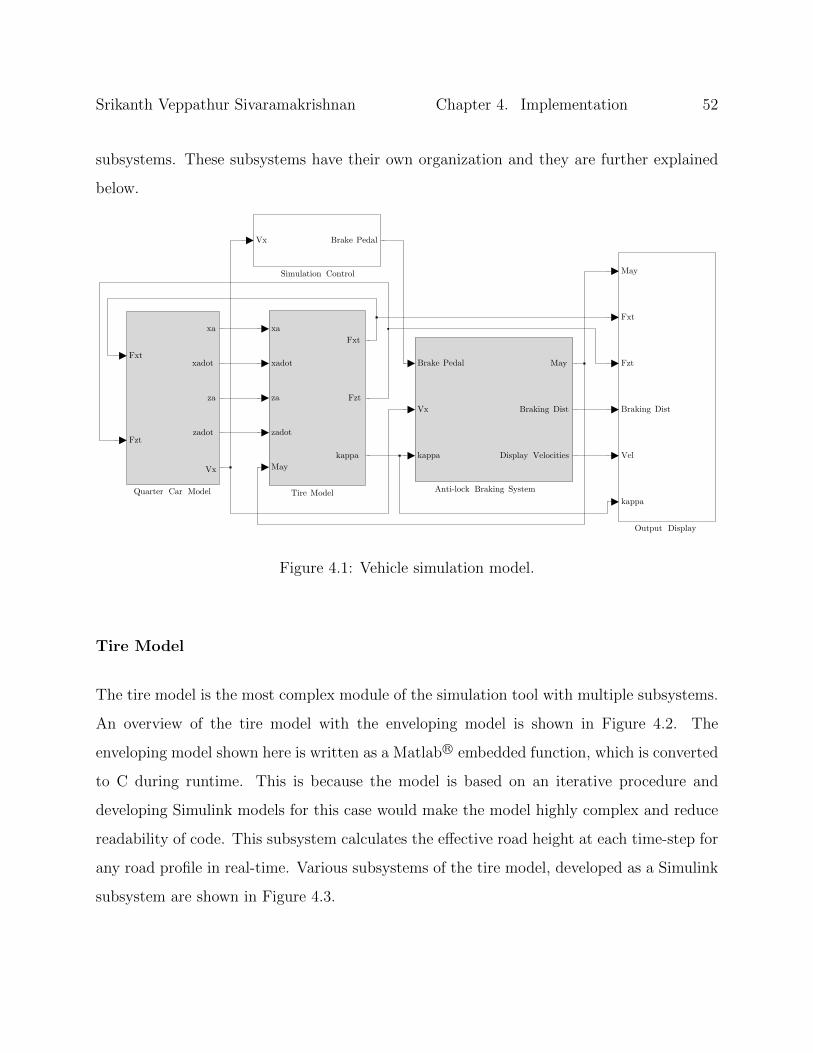
Srikanth Veppathur Sivaramakrishnan Chapter 4. Implementation 52
subsystems. These subsystems have their own organization and they are further explained
below.
Tire Model
xa
xadot
za
zadot
May
Fxt
Fzt
kappa
Simulation Control
Vx Brake Pedal
Vx
Quarter Car Model
Fxt
Fzt
xa
xadot
za
zadot
Output Display
May
Fxt
Fzt
Braking Dist
Vel
kappaAnti-lock Braking System
Brake Pedal
Vx
kappa
May
Braking Dist
Display Velocities
Figure 4.1: Vehicle simulation model.
Tire Model
The tire model is the most complex module of the simulation tool with multiple subsystems.
An overview of the tire model with the enveloping model is shown in Figure 4.2. The
enveloping model shown here is written as a Matlab R© embedded function, which is converted
to C during runtime. This is because the model is based on an iterative procedure and
developing Simulink models for this case would make the model highly complex and reduce
readability of code. This subsystem calculates the effective road height at each time-step for
any road profile in real-time. Various subsystems of the tire model, developed as a Simulink
subsystem are shown in Figure 4.3.
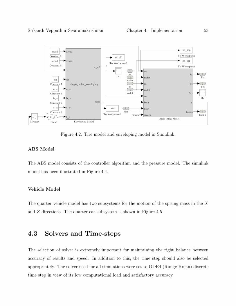
Srikanth Veppathur Sivaramakrishnan Chapter 4. Implementation 53
kappa3
Fzt2
Fxt1
w
za_inp
To Workspace4
xa_inp
To Workspace3w_eff
To Workspace2
beta
To Workspace1
Rigid Ring Model
xa
xadot
za
zadot
zw
beta
May
omega
Fx
Fz
My
a
kappa
My
Memory Gain3
2* p_ls
Enveloping Model
zroad
xroad
x
dx
a_e
b_e
c_e
l_s
w_eff
beta
single_point_enveloping
Constant 9
zroad
Constant 8
xroad
Constant 7
dx
Constant 6
c_e
Constant 5
b_e
Constant 4
a_e
omegaMay5
zadot4za3
xadot2xa1
Figure 4.2: Tire model and enveloping model in Simulink.
ABS Model
The ABS model consists of the controller algorithm and the pressure model. The simulink
model has been illustrated in Figure 4.4.
Vehicle Model
The quarter vehicle model has two subsystems for the motion of the sprung mass in the X
and Z directions. The quarter car subsystem is shown in Figure 4.5.
4.3 Solvers and Time-steps
The selection of solver is extremely important for maintaining the right balance between
accuracy of results and speed. In addition to this, the time step should also be selected
appropriately. The solver used for all simulations were set to ODE4 (Runge-Kutta) discrete
time step in view of its low computational load and satisfactory accuracy.
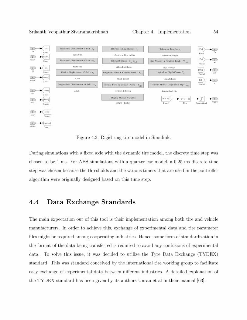
Srikanth Veppathur Sivaramakrishnan Chapter 4. Implementation 54
kappa5
a4
My3
Fz2
Fx1
Vertical Displacement of Belt - zb
z-belt
Longitudinal Displacement of Belt - xb
x-belt
Normal Force in Contact Patch - FcN
vertical deflection
Rotational Displacement of Axle - θa
theta-rim
Rotational Displacement of Belt - θb
theta-belt
Slip Velocity in Contact Patch - Vcsx
slip velocity
Longitudinal Slip Stiffness - Cκ
slip stiffness
Sidewall Stiffness - Cb, Cbθ
sidewall stiffness
Relaxation Length - σc
relaxation length
Display Output Variables
output display
Transient Model - Longitudinal Slip - ζcx
longitudinal slip
Effective Rolling Radius - re
effective rolling radius
Tangential Force in Contact Patch - FcT
brush model
Saturation1
Goto7
omega
Goto6
beta
Goto5
zw
Goto4
May
Goto3
zadot
Goto2
za
Goto1
xadot
Goto
xa
From8
slip_cx
From3
a
From2
My
From1
Fz
From
Fx
Fcn
-u/ (1+ u)
omega8
May7
beta6
zw5
zadot
za3
xadot2
xa1
4
Figure 4.3: Rigid ring tire model in Simulink.
During simulations with a fixed axle with the dynamic tire model, the discrete time step was
chosen to be 1 ms. For ABS simulations with a quarter car model, a 0.25 ms discrete time
step was chosen because the thresholds and the various timers that are used in the controller
algorithm were originally designed based on this time step.
4.4 Data Exchange Standards
The main expectation out of this tool is their implementation among both tire and vehicle
manufacturers. In order to achieve this, exchange of experimental data and tire parameter
files might be required among cooperating industries. Hence, some form of standardization in
the format of the data being transferred is required to avoid any confusions of experimental
data. To solve this issue, it was decided to utilize the Tyre Data Exchange (TYDEX)
standard. This was standard conceived by the international tire working group to facilitate
easy exchange of experimental data between different industries. A detailed explanation of
the TYDEX standard has been given by its authors Unrau et al in their manual [63].

Srikanth Veppathur Sivaramakrishnan Chapter 4. Implementation 55
2Braking Dist
May1cont roller_ flag
brk_pdl
flag_FL
flag_FR
flag_RL
flag_RR
Switch1
Pressure Model
Master Cylinder Pressure
epsilon
Brake State
m1
Brake Pressure
Master Cylinder
brake pedal pm
Integrator1
1/ s
Gain1
Cp_f
Control Algorithm
Brake Pedal
Ctlr Flag
epsilon_t
Vx
kappa
epsilon
Brake State
m1
Constant
0
kappa4
Vx3
epsilon2
1Brake Pedal
Figure 4.4: ABS subsystem.
Vx5
zadot4
za3
xadot2
xa1
Z-Axis
Fzt
zadot
za
X -Axis
Fxt
xadot
xa
Vehicle_Vx
Fzt2
Fxt1
Figure 4.5: Quarter car model in Simulink.
In this study, the capability to read experimental data and parameter values of tires from
standard TYDEX files was incorporated to reduce the additional effort involved in the im-
plementation of the tool and its work-flow integration. This would also ensure backward
compatibility and with parameter files from other simulation software such as MF-SWIFT
which utilize the same standard.
Srikanth Veppathur Sivaramakrishnan Chapter 4. Implementation 56
4.5 Model Optimization
When the simulation model was developed and implemented in their current state, it was
realized that the performance might not be optimal and feature set might be limited. An
important point of concern was that the speed of computation in each subsystem needed
to be maintained to ensure it does not slow down the entire simulation. The following
optimizations were done to improve the speed of simulation results:
• During initial test runs it was observed that the iterative calculations in the enveloping
model was slowing down the entire simulation. This was due to the fact that a process
of extrapolation was taking place at every time step. This was then replaced with an
indexed array with the road height and horizontal position at fixed intervals. Based
on this, the road profile at each time step was approximated to the nearest available
point instead of extrapolation. This modification has shown good improvements in the
speed of results.
• The scan width of the enveloping model has been set to [−ae/6, ae/6] to balance
between accuracy and achieving faster results without spending computational effort
on a bigger scan interval.
• The relaxation length has been approximated using Equation (3.30) to reduce the
numerical load in calculating slip stiffness at each time step.
• The calculation of wheel slip κ and wheel acceleration ε for the ABS model has been
done based the theoretical slip ζcx to match the rotating coordinate system being used
in the tire model and the global coordinate system used in the ABS model.
• All functions used in the simulink model were chosen based on their ability to be
converted into equivalent C-functions. This was done keeping future extensions in
mind for developing standalone applications.

Srikanth Veppathur Sivaramakrishnan Chapter 4. Implementation 57
• After completing the construction of the Simulink model and finalizing model param-
eters, the simulation file was converted into a Matlab R© MEX function, which is a
C-compiled executable of the Simulink file. This was found to significantly improve
the efficiency of calculations and reduce simulation time.
• All definitions of model parameter constants such as automated extraction from tire
parameter (TIR) files, simulation runs and plotting of results were performed using
scripts instead of a Graphical User Interface (GUI) based approach to reduce the
amount of user intervention required inside the model and to provide a code frame-
work for automated iterations of simulation runs under various test cases for ABS
development.
4.6 Conclusions
The simulation model of a quarter car with an ABS system using a dynamic tire model was
successfully developed in Matlab-Simulink R©. These models were further modified for opti-
mum performance and a code framework has been developed for the automated processing
of tire parameter files and conducting simulation runs. Following this, a model parameter-
ization process was developed and simulation runs were conducted for multiple test cases,
which are explained in subsequent chapters.

Chapter 5
Model Parameterization
The mathematical model of the dynamic tire involves multiple parameters that are either
physical quantities such as sidewall stiffness, damping etc. and also curve fitting parameters
to model the non-linear relationships between certain quantities. This chapter describes in
detail the procedure developed to parameterize the rigid ring tire model and the enveloping
model. Major parts of the procedure and the initial analysis was based on the methods
described by Besselink [5] and Schmeitz et al [64]. Also, the Curve Fitting ToolboxTM
available in Matlab R© has been utilized for the development of the fitting algorithm.
5.1 Reference Tire
In this study, a specific tire was selected as a reference for parameterization and analysis
based on the availability of experimental data and available tire parameters. The dimensions
of the tire used in this study is denoted as a Goodyear 205/60R15 91V where the numbers
are described, and illustrated by Zegelaar [1] in Figure 5.1 and explained in Table 5.1.
58

Srikanth Veppathur Sivaramakrishnan Chapter 5. Model Parameterization 59
Notation Meaning
205 Section width in mm
60 Ratio between section height and width in % (aspect ratio)
R Radial tire
15 Rim diameter in inches
91 Maximum allowable load on the tire - 6030 N (load index)
V Speed rating - 240 km/h
Table 5.1: Reference tire notation
5.2 Experimental Procedure
The physical and empirical parameters of the tire model used in this study are either through
direct measurements or based on fitting experimental data. This data is obtained using
standard test procedures and measurement conventions. The following experiments are
required to be performed in order to completely parameterize the dynamic tire model:
• Geometric and inertial measurements.
• Steady-state longitudinal force vs. slip characteristics.
• Vertical load vs. deflection at multiple inflation pressures.
• Loaded radius, effective rolling radius vs. vertical load and forward velocity at multiple
inflation pressures.
• Rolling resistance force vs. forward velocity at various values of inflation pressure.
• Contact patch length vs. vertical load.
• Low-speed enveloping tests on different types of cleats on a fixed axle at multiple loads.
• High-speed cleat tests at different velocities using a fixed axle.

Srikanth Veppathur Sivaramakrishnan Chapter 5. Model Parameterization 60
tread widthsection width
sectionheight
outerdiameter
rim diameter
Figure 5.1: Tire dimensions. Adapted from Zegelaar, P. (1998). The dynamic response of
tyres to brake torque variations and road unevennesses. Delft University of Technology. Used
under fair use, 2013.
Generally, experiments that require multiple loads and inflation pressures are based on three
distinct values for each, totaling nine experiments. In cases where only one inflation pressure
is required, the nominal pressure P0 is used. Table 5.2 shows the various measurement points
used for obtaining data in this study. Here, LI refers to the load index.
Parameter Values
Vertical load
L1 = 0.4 · LIL2 = 0.8 · LIL3 = 1.2 · LI
Inflation pressure
P1 = P0 − 0.5 bar
P2 = P0
P3 = P0 + 0.5 bar
Table 5.2: Measurements points for multiple loads and inflation pressures
Since the in-plane dynamics are of major focus in this study, the camber angle and side-slip
angle were always set to zero as a pre-condition before performing the experiments. All the

Srikanth Veppathur Sivaramakrishnan Chapter 5. Model Parameterization 61
experimental data used in this study were obtained from a trial version of TNO MF-Tool
6.1 [65]. Detailed descriptions of collected experimental data has been provided in their
documentation [66].
5.2.1 Nominal Parameters
Before beginning the parameterization process, a set of nominal values need to be fixed
for the operating conditions for the tire to ensure that the tire is not used at values that
extremely deviate from the nominal set. These would also be used to convert tire parameters
into non-dimensional quantities. Their selection is very important because the measurement
points are based on them and they need to be fixed throughout the parameterization process.
The parameters for the reference tire used in this study are shown in Table 5.3.
Parameter Symbol Value
Inflation pressure P0 2.2 bar
Vertical load Fz0 4000 N
Rolling velocity Vx0 16.7 m/s
Table 5.3: Nominal parameters for the tire
5.2.2 Inertial and Dimensional Parameters
The major inertial parameters of the tire used in the model involve the mass mb and rota-
tional moment of inertia Iby of the belt along the Y -axis. These are directly measured through
experiments. The main dimensional parameter includes the unloaded radius r0 is also mea-
sured directly. The standard procedure adopted for these measurements are explained in
SAE J2717 [67]. In the case of absence of experimental data, the following empirical values
are assigned for the tire belt inertial parameters:
75% of the tire mass is considered to be belt mass mb
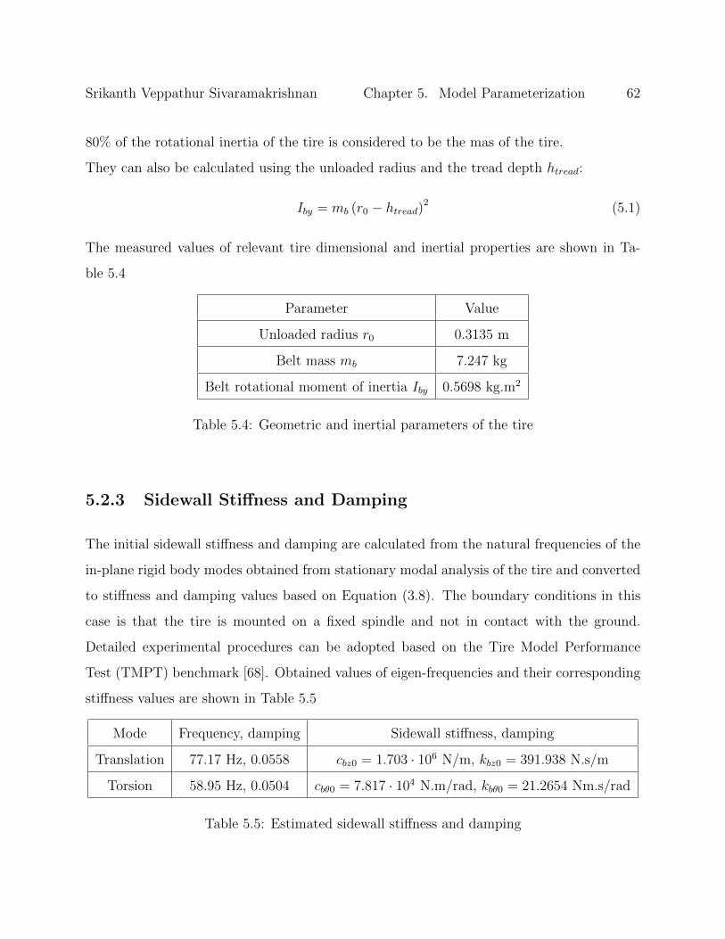
Srikanth Veppathur Sivaramakrishnan Chapter 5. Model Parameterization 62
80% of the rotational inertia of the tire is considered to be the mas of the tire.
They can also be calculated using the unloaded radius and the tread depth htread:
Iby = mb (r0 − htread)2 (5.1)
The measured values of relevant tire dimensional and inertial properties are shown in Ta-
ble 5.4
Parameter Value
Unloaded radius r0 0.3135 m
Belt mass mb 7.247 kg
Belt rotational moment of inertia Iby 0.5698 kg.m2
Table 5.4: Geometric and inertial parameters of the tire
5.2.3 Sidewall Stiffness and Damping
The initial sidewall stiffness and damping are calculated from the natural frequencies of the
in-plane rigid body modes obtained from stationary modal analysis of the tire and converted
to stiffness and damping values based on Equation (3.8). The boundary conditions in this
case is that the tire is mounted on a fixed spindle and not in contact with the ground.
Detailed experimental procedures can be adopted based on the Tire Model Performance
Test (TMPT) benchmark [68]. Obtained values of eigen-frequencies and their corresponding
stiffness values are shown in Table 5.5
Mode Frequency, damping Sidewall stiffness, damping
Translation 77.17 Hz, 0.0558 cbz0 = 1.703 · 106 N/m, kbz0 = 391.938 N.s/m
Torsion 58.95 Hz, 0.0504 cbθ0 = 7.817 · 104 N.m/rad, kbθ0 = 21.2654 Nm.s/rad
Table 5.5: Estimated sidewall stiffness and damping

Srikanth Veppathur Sivaramakrishnan Chapter 5. Model Parameterization 63
Zegelaar [1] observed that the stiffness values estimated through stationary modal analysis
might be too high due to the fact that the stiffness during rolling is less and Dorfi [69] observed
there is a shift in the modal frequencies due to the cycling of rubber and material transport.
Hence, a correction factor is recommended to account for such rolling effects, as shown in
Equation (3.9). These factors can be determined through an optimization procedure through
experimental results obtained from cleat testing. In this study, these correction factors were
set to empirical values: qbV x = 0.3640 and qbV θ = 0.0648.
5.2.4 Vertical Stiffness
The total vertical stiffness of the tire is determined through the variation of vertical deflection
vs. load on the tire. In this study, the deflection test has been performed on a rolling tire
at different velocities and inflation pressure. Hence, the deflection is calculated using the
loaded radius of the tire. As a first step, the fitting parameters qV 2, qFz1 and qFz2 were
evaluated using data obtained at nominal pressure P0 using non-linear curve fitting as shown
in Figure 5.2:
Fz =
(1 + qV 2
Ω · r0
V0
)· Fz0 ·
(qFz1
ρ
r0
+ qFz2
(ρ
r0
)2)
(5.2)
Based on this, the total vertical stiffness is calculated using Equation (3.24). The effect of
inflation pressure is then captured through an additional factor pFz1 with data measured at a
given vertical deflection (loaded radius) ρ = 0.0128 m at multiple loads and rolling velocities
using non-linear curve fitting as shown in Figure 5.3:
Fz =
(1 + qV 2
Ω · r0
V0
)· Fz0 ·
(qFz1
ρ
r0
+ qFz2
(ρ
r0
)2)
(1 + pFz1 · dP ) (5.3)
The calculated parameter values are shown in Table 5.6. SAE J2704 [70] can be used for
standardized measurement of normal force vs. deflection characteristics without any speed
effects. When no experimental data is available, a vertical stiffness Cz0 is used with qFz2 = 0.

Srikanth Veppathur Sivaramakrishnan Chapter 5. Model Parameterization 64
Measurement
Fit
Verticalload
(N)
Vertical deflection (m) Angular velocity (rad/s)
4060
80100
120
0.02
0.03
0.04
2000
4000
6000
8000
10000
Figure 5.2: Loaded radius measurements at P = 2.2 bar.
5.2.5 Effective Rolling Radius
The parameters for effective rolling radius are based on the same experimental data obtained
for loaded radius analysis. The calculation of rolling radius is based on an empirical approach
through Equation (3.22). The parameters Breff , Dreff , Freff , qre0 and qV 1 are calculated
based on the variation of the effective rolling radius with load and forward velocity using a
non-linear surface fitting procedure. This method assists in capturing the load dependency
and the growth in tire radius due to centrifugal forces.
Figure 5.4 shows the final results of the surface fit and the estimated parameters are shown in
Table 5.7. In the absence of measurements for effective rolling radius, the following empirical
values are suggested for a radial tire: Breff = 8, Dreff = 0.24, Freff = 0.01, qre0 = 1, qV 1 = 0.
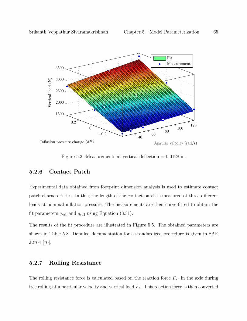
Srikanth Veppathur Sivaramakrishnan Chapter 5. Model Parameterization 65
Measurement
Fit
Verticalload
(N)
Inflation pressure change (dP ) Angular velocity (rad/s)
4060
80100
120
−0.2
0
0.2
1500
2000
2500
3000
3500
Figure 5.3: Measurements at vertical deflection = 0.0128 m.
5.2.6 Contact Patch
Experimental data obtained from footprint dimension analysis is used to estimate contact
patch characteristics. In this, the length of the contact patch is measured at three different
loads at nominal inflation pressure. The measurements are then curve-fitted to obtain the
fit parameters qra1 and qra2 using Equation (3.31).
The results of the fit procedure are illustrated in Figure 5.5. The obtained parameters are
shown in Table 5.8. Detailed documentation for a standardized procedure is given in SAE
J2704 [70].
5.2.7 Rolling Resistance
The rolling resistance force is calculated based on the reaction force Fxr in the axle during
free rolling at a particular velocity and vertical load Fz. This reaction force is then converted

Srikanth Veppathur Sivaramakrishnan Chapter 5. Model Parameterization 66
Parameter Value
Cz0 1.90 · 105 N/m
qFz1 12.6762
qFz2 15.2315
qV 2 0.0740
pFz1 0.7064
Table 5.6: Estimated vertical stiffness parameters
Parameter Value
Breff 2.1733
Dreff 0.2140
Freff 0.0567
qre0 0.9822
qV 1 7.4026 · 10−4
Table 5.7: Estimated parameters for effective rolling radius
to the rolling resistance coefficient fr using the relation:
fr =FxrFz
(5.4)
Equation (3.33) is then used to obtain a fit for the velocity and pressure dependence of
rolling resistance coefficient. Figure 5.6 shows the non-linear surface fit results and the
estimated parameters are shown in Table 5.9. ISO standards [71] are required to be followed
Parameter Value
qra1 0.6390
qra2 0.6625
Table 5.8: Estimated parameters for the contact patch

Srikanth Veppathur Sivaramakrishnan Chapter 5. Model Parameterization 67
Measurement
Fit
Effectiverollingradius(m
)
Vertical load (N) Angular velocity (rad/s)
4060
80100
120
4000
6000
8000
0.285
0.29
0.295
0.3
0.305
0.31
Figure 5.4: Effective rolling radius measurements at 2.2 bar
for measuring rolling resistance.
Parameter Value
qsy1 0.0070
qsy3 0.0016
qsy4 9.420 · 10−5
qsy8 -0.3189
Table 5.9: Estimated parameters for rolling resistance
5.2.8 Tread Element Stiffness
The tread element stiffness cpx per unit length is the main parameter involved in the calcula-
tion of steady-state tangential forces using the brush model as described in Equation (3.25).
This parameter is assumed to be invariable with pressure and is determined from the steady-

Srikanth Veppathur Sivaramakrishnan Chapter 5. Model Parameterization 68
Curve fit
Measurement
half-lengthof
contact
patch
(m)
Vertical load (N)
0 1000 2000 3000 4000 5000 60000
0.01
0.02
0.03
0.04
0.05
0.06
0.07
0.08
0.09
Figure 5.5: Contact patch length vs. vertical load at 2.2 bar.
state longitudinal force vs slip characteristics of the tire using the relation:
cpx =Cκ0
2a2(5.5)
where Cκ0 is the slip stiffness of the tire at free rolling condition which is the slope of
the force-slip curve at κ = 0. This is calculated from experimentally obtained force-slip
characteristics, as shown in Figure 5.7. Alternatively, this data can also be used for fit the
Magic Formula [6] if one chooses to use this instead of the brush model.
The half-length of the contact patch a is calculated using Equation (3.31) after accounting
for the effect of inflation pressure on the vertical stiffness Cz. The calculated value of tread
element stiffness per unit length is shown in Table 5.10.

Srikanth Veppathur Sivaramakrishnan Chapter 5. Model Parameterization 69
Measurement
Fit
Rollingresistan
cecoeffi
cient
Inflation pressure (bar) Forward velocity (m/s)
1015
2025
30
2
2.5
3
×10−3
6
8
10
12
Figure 5.6: Variation of rolling resistance.
Parameter Value
cpx 10.934 · 106 N/m2
Table 5.10: Estimated value of tread element stiffness
5.2.9 Enveloping Characteristics
The parameters of the enveloping model primarily involve the dimensions and the order of the
tandem elliptical cams. This is the most computationally heavy procedure in comparison to
all others because it involves an optimization procedure where the ellipse shape parameters
are changed with each iteration and compared with experimental results. The obtained
effective height for three types of cleats at different loads is shown in Figure 5.8. To obtain
this data, the tire is inflated to nominal pressure and rolled slowly (< 1 km/h) over different
sets of cleats at a constant axle height. The reaction forces Fx, Fz at the axle are recorded

Srikanth Veppathur Sivaramakrishnan Chapter 5. Model Parameterization 70
P = 2.7 bar
P = 2.2 bar
P = 1.7 barLon
gitudinal
Force
-Fx(N
)
Longitudinal Slip κ
−1 −0.8 −0.6 −0.4 −0.2 0 0.2 0.4 0.6 0.8 1−8000
−6000
−4000
−2000
0
2000
4000
6000
8000
Fz = 2000 N
Fz = 4000 N
Fz = 6000 N
Figure 5.7: Steady-state force vs. slip characteristics.
and are used to obtain the effective road height and plane angle as:
w =Fz − Fz0Cz0
(5.6a)
β = arctan
(FxFz
)(5.6b)
The values of w and β are then optimized with the enveloping model to find the shape
parameters of the ellipse. This is done using a non-linear least squares fit of the enveloping
function to the experimental data. Since the dimensions of the ellipse are generally the
same size of the tire, the starting values are assumed to be ae = r0, be = r0, ce = 1.8
and pls = 0.8. The current procedure is designed in such a way that the most minimal
set of enveloping data is used for parameterization. Hence, only set of experimental data
is used for estimation. This can be improved using multiple sets of experimental data and
weighting factors to calculate an optimal set of parameters. From the results of the fitting
procedure shown in Figure 5.9, we can see that the enveloping model is able to closely match
experimental results. The estimated parameters are shown in Table 5.11.
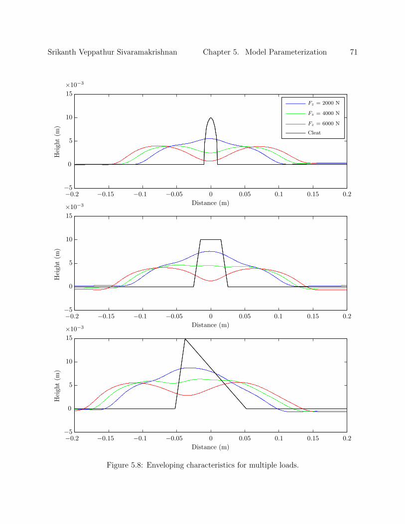
Srikanth Veppathur Sivaramakrishnan Chapter 5. Model Parameterization 71
Cleat
Fz = 6000 N
Fz = 4000 N
Fz = 2000 N
Heigh
t(m
)
Distance (m)
Heigh
t(m
)
Distance (m)
Heigh
t(m
)
Distance (m)
−0.2 −0.15 −0.1 −0.05 0 0.05 0.1 0.15 0.2
−0.2 −0.15 −0.1 −0.05 0 0.05 0.1 0.15 0.2
−0.2 −0.15 −0.1 −0.05 0 0.05 0.1 0.15 0.2
×10−3
×10−3
×10−3
−5
0
5
10
15
−5
0
5
10
15
−5
0
5
10
15
Figure 5.8: Enveloping characteristics for multiple loads.

Srikanth Veppathur Sivaramakrishnan Chapter 5. Model Parameterization 72
Measurement
Fit
Cleat
Heigh
t(m
)
Distance (m)
−0.1 −0.05 0 0.05 0.1 0.15
×10−3
−5
0
5
10
15
Figure 5.9: Enveloping model fit with experimental data.
An alternative approach towards parameterization of the enveloping model to reduce errors is
to fit the enveloping model based on reaction forces rather than through direct calculations.
Although this method tends to yield better results, the computational load is much higher
due to the fact that this process requires a full simulation at each time-step.
Parameter Value
ae 0.3626 m
be 0.3580 m
ce 1.7359
pls 0.8000
Table 5.11: Estimated parameters for the enveloping model
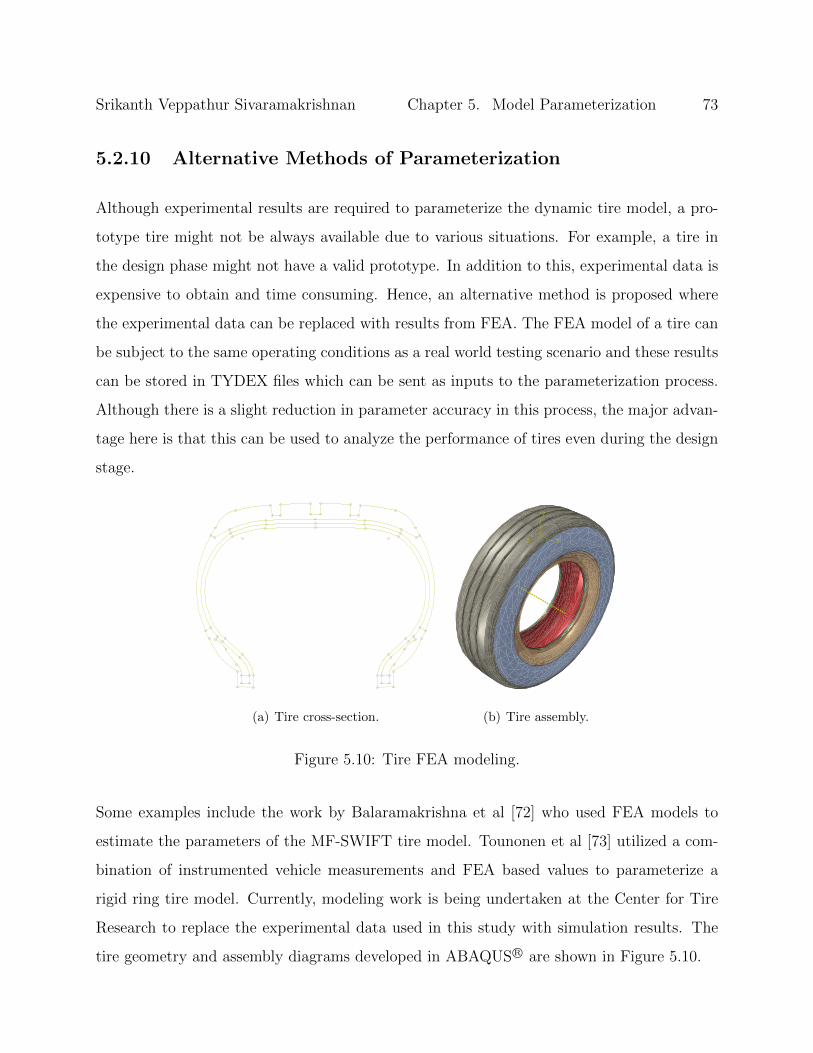
Srikanth Veppathur Sivaramakrishnan Chapter 5. Model Parameterization 73
5.2.10 Alternative Methods of Parameterization
Although experimental results are required to parameterize the dynamic tire model, a pro-
totype tire might not be always available due to various situations. For example, a tire in
the design phase might not have a valid prototype. In addition to this, experimental data is
expensive to obtain and time consuming. Hence, an alternative method is proposed where
the experimental data can be replaced with results from FEA. The FEA model of a tire can
be subject to the same operating conditions as a real world testing scenario and these results
can be stored in TYDEX files which can be sent as inputs to the parameterization process.
Although there is a slight reduction in parameter accuracy in this process, the major advan-
tage here is that this can be used to analyze the performance of tires even during the design
stage.
(a) Tire cross-section.
Z
Y
X
(b) Tire assembly.
Figure 5.10: Tire FEA modeling.
Some examples include the work by Balaramakrishna et al [72] who used FEA models to
estimate the parameters of the MF-SWIFT tire model. Tounonen et al [73] utilized a com-
bination of instrumented vehicle measurements and FEA based values to parameterize a
rigid ring tire model. Currently, modeling work is being undertaken at the Center for Tire
Research to replace the experimental data used in this study with simulation results. The
tire geometry and assembly diagrams developed in ABAQUS R© are shown in Figure 5.10.

Srikanth Veppathur Sivaramakrishnan Chapter 5. Model Parameterization 74
5.3 Conclusions
A parameterization procedure for the rigid ring tire model and enveloping model based on
non-linear curve fitting has been developed in this chapter and the model parameters were
estimated. This is shown in Figure 5.11.
Sidewall stiffness and
damping
Experimental
data
Nominal
parameters
0 0 0, ,
zP F V
θ θ0 0 0, 0 0 0, , , ,
bx bz b bx bz bc c c k k k
Vertical stiffness
1 1 2 0 2, ,, ,
Fz Fz Fz z VCp qq q
Contact patch
length
1 2,
ra raq q
Tread element
stiffness
pxc
Rolling
resistance
1 3 4 8, , ,
sy sy sy syq q q q
Inertial and geometric
parameters
0, ,b bym I r
Effective rolling
radius
0 1, ,, ,reff reff reff re VB qF qD
Enveloping model
, , ,e e e lsa cb p
Figure 5.11: Procedure for parameter estimation.
Work on alternative approaches that would supplant experimental data were also explained.
The parameters estimated for a 205/60R15 tire based on the current procedure are found to
have good correlation with the parameters for the same tire mentioned in literature [5] with
an acceptable margin of difference. There is more scope for improvement in the determination
of dynamic sidewall stiffness. Subsequent chapters concentrate on the analysis of simulation
results and conclusions from them.

Chapter 6
Results and Validation
In order to establish the reliability of the model it is necessary to compare and validate the
accuracy of simulation results with experimental data. This chapter explains the validation
of the tire model which was done using experimental data available for both high-speed
cleat tests and low-speed enveloping tests over different types of cleats. Following this, the
complete simulation model with all the components are subjected to various test cases and
the results are analyzed.
6.1 Enveloping Model Validation
The validation of the enveloping model involves comparison of the calculations of the effective
road profile with actual measurements. For this, the ellipse shape parameters which were
obtained in Section 5.2.9 were used to calculate the effective road profile height w and slope
β at various vertical loads for three types of cleats: 1. Cylindrical; 2. Trapezoidal and 3.
Triangular. It was ensured that the experimental data used for validation studies were not
previously used for model parameterization and all tests were conducted at nominal inflation
pressure. The test results are shown in Figures 6.1, 6.2 and 6.3.
75

Srikanth Veppathur Sivaramakrishnan Chapter 6. Results and Validation 76
Measurement
Simulation
Cleat
β(rad
)
Distance (m)
w(m
)
Distance (m)
−0.1 −0.05 0 0.05 0.1 0.15
−0.1 −0.05 0 0.05 0.1 0.15
×10−3
−0.2
0
0.2
−5
0
5
10
15
Figure 6.1: Enveloping over a cylindrical cleat at Fz = 2000 N.
Measurement
Simulation
Cleat
β(rad
)
Distance (m)
w(m
)
Distance (m)
−0.1 −0.05 0 0.05 0.1 0.15
−0.1 −0.05 0 0.05 0.1 0.15
×10−3
−0.1
0
0.1
−5
0
5
10
15
Figure 6.2: Enveloping over a trapezoidal cleat at Fz = 4000 N.
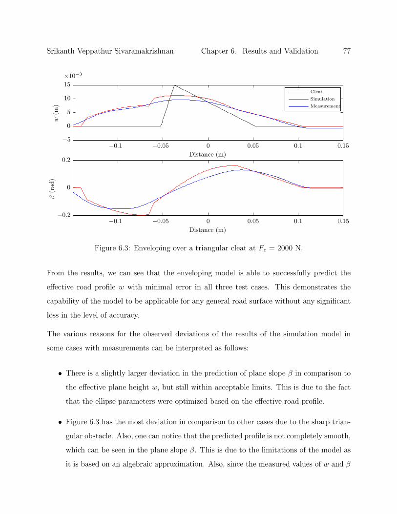
Srikanth Veppathur Sivaramakrishnan Chapter 6. Results and Validation 77
Measurement
Simulation
Cleat
β(rad
)
Distance (m)
w(m
)
Distance (m)
−0.1 −0.05 0 0.05 0.1 0.15
−0.1 −0.05 0 0.05 0.1 0.15
×10−3
−0.2
0
0.2
−5
0
5
10
15
Figure 6.3: Enveloping over a triangular cleat at Fz = 2000 N.
From the results, we can see that the enveloping model is able to successfully predict the
effective road profile w with minimal error in all three test cases. This demonstrates the
capability of the model to be applicable for any general road surface without any significant
loss in the level of accuracy.
The various reasons for the observed deviations of the results of the simulation model in
some cases with measurements can be interpreted as follows:
• There is a slightly larger deviation in the prediction of plane slope β in comparison to
the effective plane height w, but still within acceptable limits. This is due to the fact
that the ellipse parameters were optimized based on the effective road profile.
• Figure 6.3 has the most deviation in comparison to other cases due to the sharp trian-
gular obstacle. Also, one can notice that the predicted profile is not completely smooth,
which can be seen in the plane slope β. This is due to the limitations of the model as
it is based on an algebraic approximation. Also, since the measured values of w and β

Srikanth Veppathur Sivaramakrishnan Chapter 6. Results and Validation 78
are obtained indirectly from the reaction forces at the axle using Equation (5.6), the
values tend to be smooth.
• The presence of minor aberrations in Figure 6.3 can be attributed to the scan width
and the shift between the ellipse which might not be optimal for all types of obstacles.
In conclusion, the enveloping model based on the current parameterization procedure is able
to successfully predict the effective road profile and slope and provide results within accept-
able error bounds. Hence, this model is used with the rigid ring tire model for validation in
subsequent sections.
6.2 Tire Model Validation
The validation of the dynamic tire model is based on experimental data of the force response
that was obtained by rolling a tire over a rectangular cleat at different vertical loads and
velocities. In all cases, the axle was kept at a constant height for loading and nominal inflation
pressure was maintained. The rectangular cleat has dimensions of 0.05 m (length) and 0.01 m
(height). The outputs measured were the reaction forces at the axle and the wheel rotational
velocity. This response is then analyzed in both time and frequency domain and compared
with experimental data. A detailed description of all procedures adopted to obtained this
dataset is given by TNO [66]. SAE J2730 [74] can be utilized as a standard procedure for
performing dynamic cleat testing. Four test cases were analyzed for the validation studies.
Four test cases were selected out of the available data and the tire model was simulated
under the same operating conditions. Figures 6.4, 6.5, 6.6 and 6.7 show the results of the
cleat tests and their comparison with simulation results. Here, the analyzed variables are
the change in longitudinal axle force ∆Fx, change in vertical axle force ∆Fz, the change in
rotational velocity ∆Ω and their respective power spectral densities SFxFx , SFzFz and SΩΩ.
The following observations can be made based on the simulation results and their comparison

Srikanth Veppathur Sivaramakrishnan Chapter 6. Results and Validation 79
SΩΩ(dB)
Frequency (Hz)
SF
zF
z(dB)
Frequency (Hz)
SF
xF
x(dB)
Frequency (Hz)
∆Ω
(rad
/s)
Time (sec)
∆Fz(N
)
Time (sec)
Measurement
Simulation
∆Fx(N
)
Time (sec)
0 50 100 150
0 50 100 150
0 50 100 150
0 0.05 0.1 0.15 0.2 0.25
0 0.05 0.1 0.15 0.2 0.25
0 0.05 0.1 0.15 0.2 0.25
−60
−40
−20
0
20
0
20
40
60
80
0
20
40
60
80
−3
−2
−1
0
1
2
3
−1000
0
1000
2000
3000
−2000
−1000
0
1000
2000
3000
Figure 6.4: Tire rolling over a rectangular cleat at 20 km/h and Fz = 2000 N.
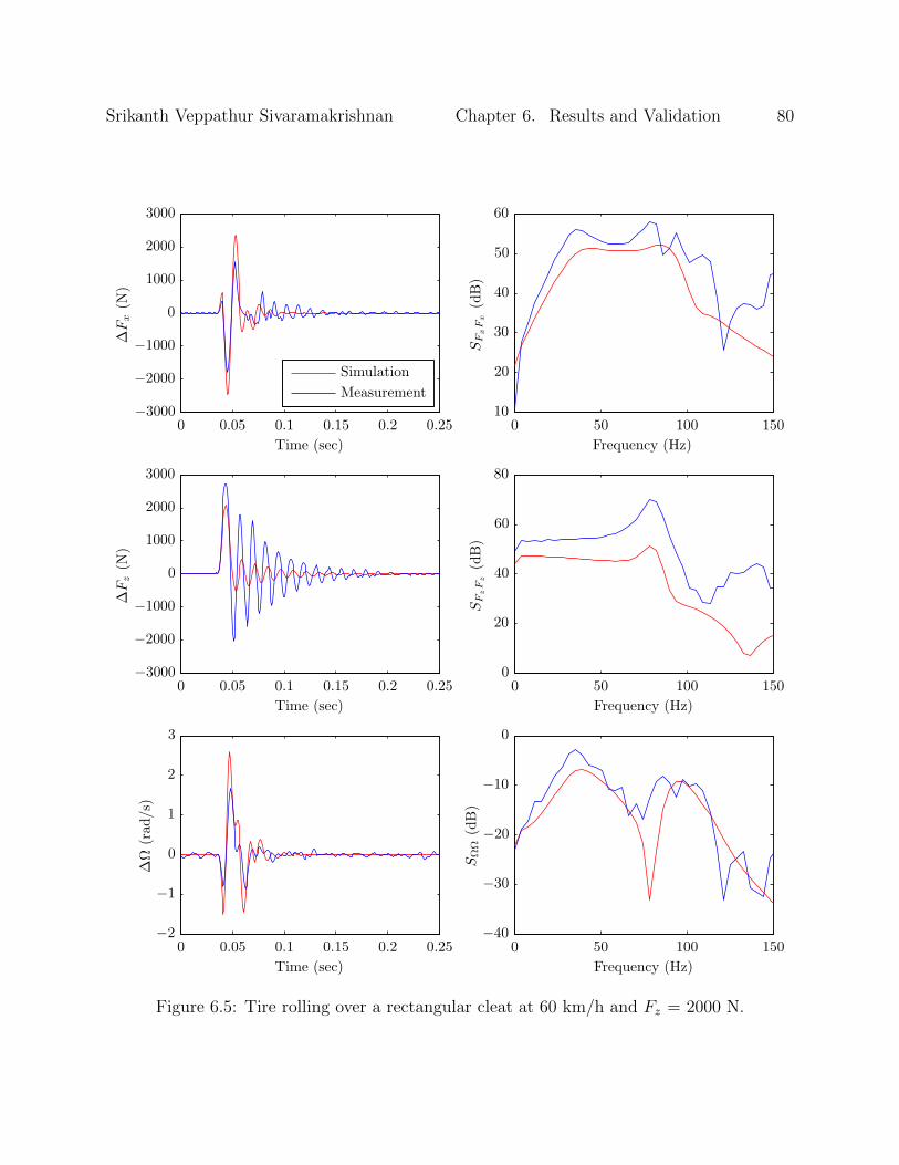
Srikanth Veppathur Sivaramakrishnan Chapter 6. Results and Validation 80
SΩΩ(dB)
Frequency (Hz)
SF
zF
z(dB)
Frequency (Hz)
SF
xF
x(dB)
Frequency (Hz)
∆Ω
(rad
/s)
Time (sec)
∆Fz(N
)
Time (sec)
Measurement
Simulation
∆Fx(N
)
Time (sec)
0 50 100 150
0 50 100 150
0 50 100 150
0 0.05 0.1 0.15 0.2 0.25
0 0.05 0.1 0.15 0.2 0.25
0 0.05 0.1 0.15 0.2 0.25
−40
−30
−20
−10
0
0
20
40
60
80
10
20
30
40
50
60
−2
−1
0
1
2
3
−3000
−2000
−1000
0
1000
2000
3000
−3000
−2000
−1000
0
1000
2000
3000
Figure 6.5: Tire rolling over a rectangular cleat at 60 km/h and Fz = 2000 N.

Srikanth Veppathur Sivaramakrishnan Chapter 6. Results and Validation 81
SΩΩ(dB)
Frequency (Hz)
SF
zF
z(dB)
Frequency (Hz)
SF
xF
x(dB)
Frequency (Hz)
∆Ω
(rad
/s)
Time (sec)
∆Fz(N
)
Time (sec)
Measurement
Simulation
∆Fx(N
)
Time (sec)
0 50 100 150
0 50 100 150
0 50 100 150
0 0.05 0.1 0.15 0.2 0.25
0 0.05 0.1 0.15 0.2 0.25
0 0.05 0.1 0.15 0.2 0.25
−40
−30
−20
−10
0
10
0
20
40
60
80
20
30
40
50
60
70
−4
−2
0
2
4
−2000
−1000
0
1000
2000
3000
−4000
−2000
0
2000
4000
Figure 6.6: Tire rolling over a rectangular cleat at 60 km/h and Fz = 4000 N.

Srikanth Veppathur Sivaramakrishnan Chapter 6. Results and Validation 82
SΩΩ(dB)
Frequency (Hz)
SF
zF
z(dB)
Frequency (Hz)
SF
xF
x(dB)
Frequency (Hz)
∆Ω
(rad
/s)
Time (sec)
∆Fz(N
)
Time (sec)
Measurement
Simulation
∆Fx(N
)
Time (sec)
0 50 100 150
0 50 100 150
0 50 100 150
0 0.05 0.1 0.15 0.2 0.25
0 0.05 0.1 0.15 0.2 0.25
0 0.05 0.1 0.15 0.2 0.25
−40
−30
−20
−10
0
10
20
10
20
30
40
50
60
70
0
20
40
60
80
−5
0
5
−2000
−1000
0
1000
2000
3000
−5000
0
5000
Figure 6.7: Tire rolling over a rectangular cleat at 60 km/h and Fz = 6000 N.

Srikanth Veppathur Sivaramakrishnan Chapter 6. Results and Validation 83
with experimental data:
• The time domain response for all four test cases except the vertical force in Figure 6.5
show comparable amplitudes of vibration and have similar settling times.
• The PSD plots show a vertical offset although the peak frequencies show a match. This
shift is minor in some plots and larger in a few, especially SFzFz in Figure 6.5. This is
due to the fact that there is lower damping predicted than measurements at low speeds
and a high damping is predicted at speeds of 60 km/h which can be attributed to the
relaxation length model with affects the relative damping. The time domain plots
reflect this effect through a phase delay between the simulations and measurements as
observed in the vertical force response of Figure 6.5.
• The time domain response for the change in horizontal force and angular velocity for
Figures 6.4 and 6.5 show good correlation with measurements. This indicates the tire
model has higher level of accuracy at lower loads.
• At higher loads of 4000 N and 6000 N, a minor deviation in measurements in the
first modal frequency for longitudinal force and angular velocity occurs. This can be
attributed to a higher predicted dynamic stiffness which is also reflected with larger
oscillations than measurements.
• The extra zeros observed in the simulation results which aren’t present in the exper-
imental data are due to the presence of null-points in the enveloping model. In this,
the calculated road profile might be zero for certain frequencies due to the geometric
setup of the tandem cams. This has been explained in detail by Schmeitz [24].
• From Figures 6.4, 6.5 and 6.7, a minor shift in the natural frequencies of the rigid
body modes of the tire at higher velocities can be seen from the experimental data.
This effect is also observed in the simulation results. This accounts for the change in
sidewall stiffness with rolling velocity.
Srikanth Veppathur Sivaramakrishnan Chapter 6. Results and Validation 84
Overall, a good correlation is observed in the response of the tire model in both time domain
and frequency domain. The predicted response and the peaks of the frequency response are
found to lie within acceptable levels of error. Hence, it can be concluded that the dynamic
tire model is valid over the specified frequency range of operation and the predicted response
lies within the expected range and error bounds.
6.3 Frequency Response to Brake Torque
Following the validation studies, it is necessary to understand the influence of in-plane dy-
namics of the tire during braking events. This is done by performing a comparison of the
simulation outputs of a quarter car model based on a Lugre transient model with the rigid
ring dynamic tire model. The Lugre model was chosen for comparison due to its widespread
usage in ABS simulations. The comparison methods used in this section is based on the
work done by Jansen [3] to understand the influence of in-plane dynamics on ABS braking.
For this analysis, an impulse braking torque May of high amplitude was chosen as an input to
the simulation models as a wide-band excitation to obtain the vertical force Fz and horizontal
force Fx at the axle and the angular velocity of the tire Ω. Due to the non-linearities of the
simulation model, the Power Spectrum Density (PSD) of the outputs SFxFx , SFzFz and SΩΩ
were obtained to plot the amplitude of the response at various frequencies, as shown in
Figure 6.8. All responses were normalized before obtaining the PSD and this results in much
smaller amplitudes.
From the results, we can see that the Lugre transient tire model matches the response of the
rigid ring model up to the wheel-hop mode. At higher frequencies above 10 Hz, the transient
model loses its validity as the amplitude of the response begins to fall. This is not seen in
the case of rigid ring model as the vertical and rotational rigid-body modes up to 100 Hz
can be seen. This demonstrates the validity of the rigid ring model over a higher frequency
range in comparison to simple transient tire models which are currently being used.

Srikanth Veppathur Sivaramakrishnan Chapter 6. Results and Validation 85
Transient tire model
Dynamic tire model
SΩΩ(dB)
Frequency (Hz)
SF
zF
z(dB)
Frequency (Hz)
SF
xF
x(dB)
Frequency (Hz)
0 50 100 150
0 50 100 150
0 50 100 150
−60
−40
−20
0
20
−60
−40
−20
0
20
−50
−40
−30
−20
−10
0
Figure 6.8: Frequency response to brake torque input.

Srikanth Veppathur Sivaramakrishnan Chapter 6. Results and Validation 86
6.4 ABS Simulations
Following the validation of the dynamic tire model, enveloping model and the understanding
that the dynamic tire model is valid over a higher frequency range in comparison to transient
tire models, simulations are required to be performed on the complete model to assess its
capabilities. This includes inducing short wavelength disturbances during ABS operation
and assessing braking performance.
6.4.1 Test cases
For this, four test cases with different road profiles were analyzed. In all test cases, the same
braking maneuver is adopted where the vehicle is assumed to be moving at 65 km/h before
the start of braking on a dry road surface of coefficient of friction µ = 0.9 to serve as a
standard for braking assessment. For experimental validation, the best practices described
in SAE J2909 [75] is recommended. The four types of road profile used for simulations in
this study are described below and shown in Figure 6.9:
Smooth Asphalt Road This is the road profile for asphalt concrete on bound base, as
shown in Figure 6.9(a) and was obtained from the Long Term Pavement Performance
(LTPP) database [76] for a stretch of highway from the state of Oklahoma. This profile
has the lowest level of disturbance and would serve as a baseline measure of braking
distance. These are measured at longer intervals of 150 mm.
Jointed Pavement Concrete Road This road profile, as shown in Figure 6.9(b) was also
obtained from the LTPP database, measured at intervals of 150 mm for a highway in
Oklahoma and this has sharper disturbances when compared to the asphalt road but
is still classified as a smooth road.
ISO Grade D Asphalt This standard road profile was available from the Center for Tire
Research and would assist in understanding the braking distance variations on a road
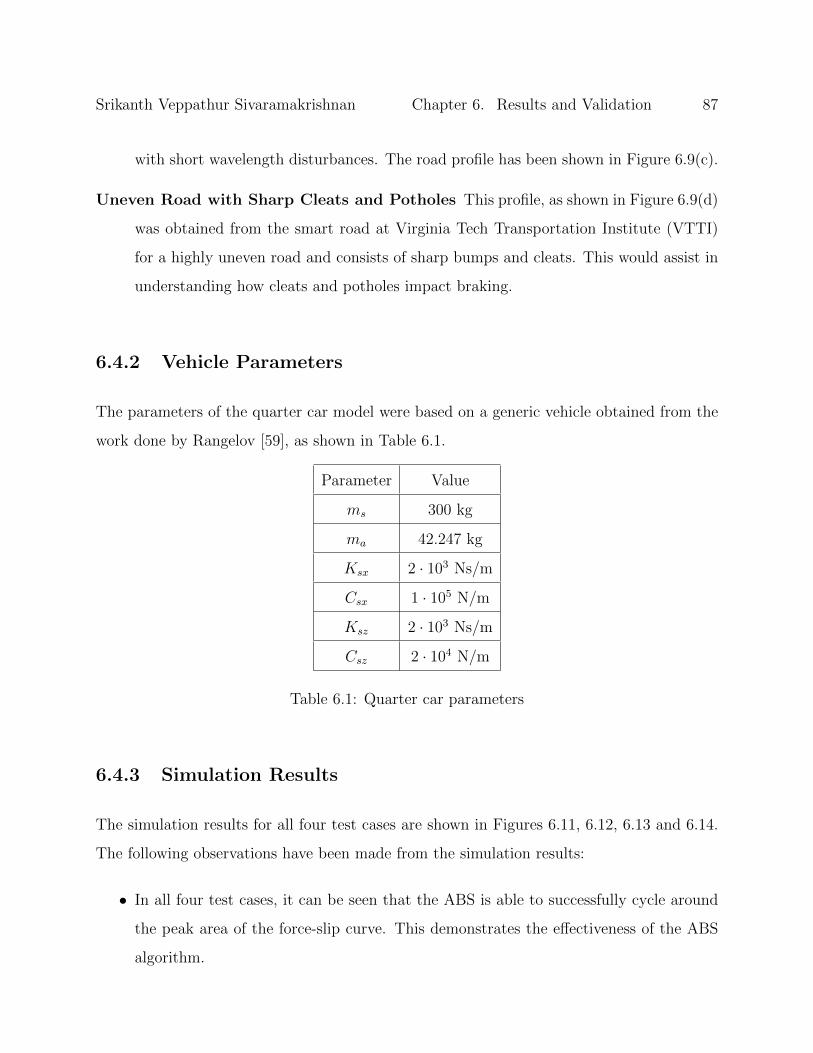
Srikanth Veppathur Sivaramakrishnan Chapter 6. Results and Validation 87
with short wavelength disturbances. The road profile has been shown in Figure 6.9(c).
Uneven Road with Sharp Cleats and Potholes This profile, as shown in Figure 6.9(d)
was obtained from the smart road at Virginia Tech Transportation Institute (VTTI)
for a highly uneven road and consists of sharp bumps and cleats. This would assist in
understanding how cleats and potholes impact braking.
6.4.2 Vehicle Parameters
The parameters of the quarter car model were based on a generic vehicle obtained from the
work done by Rangelov [59], as shown in Table 6.1.
Parameter Value
ms 300 kg
ma 42.247 kg
Ksx 2 · 103 Ns/m
Csx 1 · 105 N/m
Ksz 2 · 103 Ns/m
Csz 2 · 104 N/m
Table 6.1: Quarter car parameters
6.4.3 Simulation Results
The simulation results for all four test cases are shown in Figures 6.11, 6.12, 6.13 and 6.14.
The following observations have been made from the simulation results:
• In all four test cases, it can be seen that the ABS is able to successfully cycle around
the peak area of the force-slip curve. This demonstrates the effectiveness of the ABS
algorithm.

Srikanth Veppathur Sivaramakrishnan Chapter 6. Results and Validation 88Heigh
t(m
)
Distance (m)
0 50 100 150 200−0.03
−0.02
−0.01
0
0.01
0.02
(a) Smooth asphalt road.
Height(m
)
Distance (m)
0 50 100 150 200
×10−3
−8
−6
−4
−2
0
2
4
6
(b) Jointed concrete pavement road.
Height(m
)
Distance (m)
0 50 100 150
×10−3
−8
−6
−4
−2
0
2
4
6
8
(c) ISO grade D asphalt road.
Heigh
t(m
)
Distance (m)
0 20 40 60 80 100−0.05
−0.04
−0.03
−0.02
−0.01
0
0.01
0.02
0.03
(d) Uneven road with sharp cleats and potholes.
Figure 6.9: Road profiles for ABS braking analysis.
• The rate of cycling of brake torque is seen to reflect real-world ABS braking scenario
as it is done at a much slower rate compared to the simulation time-step.
Srikanth Veppathur Sivaramakrishnan Chapter 6. Results and Validation 89
• Variations in the vertical force Fzt are observed to have a direct effect on the braking
force Fxt generated by the tire at the axle. This effect can be clearly seen in Fig-
ure 6.9(d) where there is a sudden drop in braking force due to the tire rolling over a
pothole.
• Short wavelength road disturbances are observed to lead to small variations in the
angular velocity which can be clearly observed in Figures 6.9(c) and 6.9(d). This is an
expected result and demonstrates the capabilities of the tire model to account for such
effects.
• From Figure 6.9(c), it is observed that sharp disturbances at longer wavelengths (large
intervals) have minimal effect on the rolling velocity of the tire although variations can
be seen in the vertical load.
• A combination of sharp cleats and large potholes with short wavelength disturbances
can be seen to have an influence towards increasing the average slip during ABS brak-
ing.
The braking distance variations for all four test cases can be seen in Figure 6.10. The
following observations have been made:
• It is observed that the presence of large cleats and potholes have a direct effect on the
braking distance of the vehicle, as seen in the case of braking distance for the uneven
road as this test case shows the greatest deviation from the baseline value of smooth
asphalt road.
• In this case, the short wavelength disturbances in the ISO grade D asphalt road has
been observed to reduce the braking distance due to higher average deflection in the
tire.
• Sharp obstacles at larger wavelengths are seen to have minimal effect on the braking
distance, as seen in the case of jointed concrete pavement road where the difference

Srikanth Veppathur Sivaramakrishnan Chapter 6. Results and Validation 90
with baseline smooth asphalt road is very less.
Based on the observations it can be concluded that the vibrations of the belt due to short
wavelength disturbances have a significant effect on the ABS braking performance of a
tire and cannot be neglected. This confirms previous studies done by Zegelaar [58] and
Pauwelussen [2]. This effect has been clearly demonstrated by the developed simulation tool
with a validated tire model.
Braking distance (m)
20 20.5 21 21.5 22
Smooth asphalt
Jointed concrete
ISO grade D asphalt
Sharp cleats and potholes
Figure 6.10: Braking distance on various road surfaces.
6.5 Conclusions
The rigid ring tire model and the elliptical cam model were successfully validated against
experimental data obtained from fixed axle tests based on the parameters calculated form
the estimation procedure and reasons for any discrepancies were analyzed. Results with
estimated parameters were found to have equal or better fit with experimental results in
comparison with parameters provided by TNO [77]. Simulations with ABS braking maneu-
vers were conducted on a quarter car model under various road surfaces and the variations
in braking distance were also analyzed.

Srikanth Veppathur Sivaramakrishnan Chapter 6. Results and Validation 91
Wheel Vcr
Vehicle Vx
VerticalforceFzt(N
)
Time (sec)
Lon
gitudinal
forceFxt(N
)
Wheel slip κ
BraketorqueM
ay(N
.m)
Time (sec)
Wheelslip
κ
Time (sec)
Lon
gitudinal
forceFxt(N
)
Time (sec)
Velocity
(m/s)
Time (sec)
2 2.5 3 3.5 4
0 0.2 0.4 0.6 0.8 1 2 2.5 3 3.5 4
2 2.5 3 3.5 4
2 2.5 3 3.5 42 2.5 3 3.5 4
3200
3300
3400
3500
3600
3700
−1000
0
1000
2000
3000
4000
0
500
1000
1500
0
0.2
0.4
0.6
0.8
1
−1000
0
1000
2000
3000
4000
0
5
10
15
20
Figure 6.11: ABS braking on smooth asphalt road.

Srikanth Veppathur Sivaramakrishnan Chapter 6. Results and Validation 92
Wheel Vcr
Vehicle Vx
VerticalforceFzt(N
)
Time (sec)
Lon
gitudinal
forceFxt(N
)
Wheel slip κ
BraketorqueM
ay(N
.m)
Time (sec)
Wheelslip
κ
Time (sec)
Lon
gitudinal
forceFxt(N
)
Time (sec)
Velocity
(m/s)
Time (sec)
2 2.5 3 3.5 4
0 0.2 0.4 0.6 0.8 1 2 2.5 3 3.5 4
2 2.5 3 3.5 4
2 2.5 3 3.5 42 2.5 3 3.5 4
3100
3200
3300
3400
3500
3600
−1000
0
1000
2000
3000
4000
0
500
1000
1500
0
0.2
0.4
0.6
0.8
1
−1000
0
1000
2000
3000
4000
0
5
10
15
20
Figure 6.12: ABS braking on jointed pavement concrete road.

Srikanth Veppathur Sivaramakrishnan Chapter 6. Results and Validation 93
Wheel Vcr
Vehicle Vx
VerticalforceFzt(N
)
Time (sec)
Lon
gitudinal
forceFxt(N
)
Wheel slip κ
BraketorqueM
ay(N
.m)
Time (sec)
Wheelslip
κ
Time (sec)
Lon
gitudinal
forceFxt(N
)
Time (sec)
Velocity
(m/s)
Time (sec)
2 2.5 3 3.5 4
0 0.2 0.4 0.6 0.8 1 2 2.5 3 3.5 4
2 2.5 3 3.5 4
2 2.5 3 3.5 42 2.5 3 3.5 4
3000
3200
3400
3600
3800
−1000
0
1000
2000
3000
4000
0
500
1000
1500
0
0.2
0.4
0.6
0.8
1
−1000
0
1000
2000
3000
4000
0
5
10
15
20
Figure 6.13: ABS braking on ISO grade D poor asphalt road.

Srikanth Veppathur Sivaramakrishnan Chapter 6. Results and Validation 94
Wheel Vcr
Vehicle Vx
VerticalforceFzt(N
)
Time (sec)
Lon
gitudinal
forceFxt(N
)
Wheel slip κ
BraketorqueM
ay(N
.m)
Time (sec)
Wheelslip
κ
Time (sec)
Lon
gitudinal
forceFxt(N
)
Time (sec)
Velocity
(m/s)
Time (sec)
2 2.5 3 3.5 4
0 0.2 0.4 0.6 0.8 1 2 2.5 3 3.5 4
2 2.5 3 3.5 4
2 2.5 3 3.5 42 2.5 3 3.5 4
0
1000
2000
3000
4000
5000
−4000
−2000
0
2000
4000
6000
8000
0
500
1000
1500
0
0.2
0.4
0.6
0.8
1
−1000
0
1000
2000
3000
4000
5000
0
5
10
15
20
Figure 6.14: ABS braking on uneven road surface with cleats and potholes.

Chapter 7
Conclusions and Future Work
The following activities have been successfully carried out in the course of this study towards
the development of a simulation tool that analyze the effect of short wavelength disturbances
and brake torque variations on ABS performance:
• A detailed literature review on the development of dynamic tire models and enveloping
models and their analysis with respect to braking performance.
• Mathematical modeling of all relevant subsystems of the simulation tool based on the
literature, including the rigid ring tire model, tandem elliptical cam enveloping model,
ABS model and quarter car model.
• Model development in Matlab-Simulink R© with relevant data exchange standards and
experimental data further optimization to improve performance.
• Development of a parameterization procedure for estimation of model parameters from
experimental data or possibly through FEA in the future.
• Validation of the dynamic tire model including the enveloping model with experimental
data from dynamic cleat tests.
95
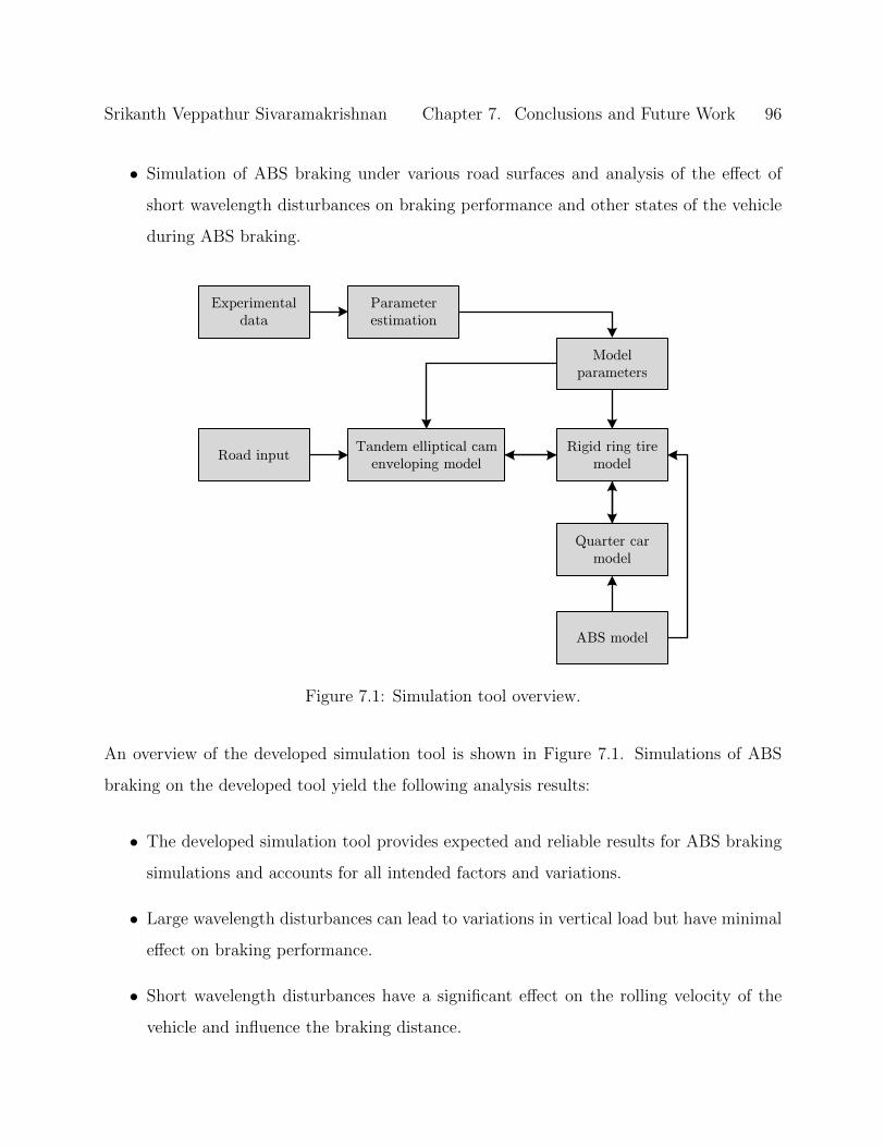
Srikanth Veppathur Sivaramakrishnan Chapter 7. Conclusions and Future Work 96
• Simulation of ABS braking under various road surfaces and analysis of the effect of
short wavelength disturbances on braking performance and other states of the vehicle
during ABS braking.
Experimental
data
Parameter
estimation
Rigid ring tire
model
Tandem elliptical cam
enveloping modelRoad input
ABS model
Quarter car
model
Model
parameters
Figure 7.1: Simulation tool overview.
An overview of the developed simulation tool is shown in Figure 7.1. Simulations of ABS
braking on the developed tool yield the following analysis results:
• The developed simulation tool provides expected and reliable results for ABS braking
simulations and accounts for all intended factors and variations.
• Large wavelength disturbances can lead to variations in vertical load but have minimal
effect on braking performance.
• Short wavelength disturbances have a significant effect on the rolling velocity of the
vehicle and influence the braking distance.
Srikanth Veppathur Sivaramakrishnan Chapter 7. Conclusions and Future Work 97
• Sharp cleats and potholes have a significant effect on the generation of braking force
and increase average slip.
7.1 Recommendations for Future Work
The various simulation models and subsystems that were developed in this study towards the
final goal of building a simulation tool have numerous scope for improvement. There is also
potential towards extending the model for other types of test cases such as ride and comfort
analysis for suspensions, evaluating active suspension controllers for robustness, stability
controller testing etc. The following recommendations are given for future work pertaining
to this study:
• Implementation of a GUI for the simulation tool that would require minimal user
intervention for conducting simulations.
• Building the simulation model as a standalone package using C/C++ that can be
deployed on any platform.
• Improving the accuracy of the procedure for parameter estimation through weighted
curve fitting using multiple sets of experimental data.
• Estimate the dynamic stiffness of the sidewall by fitting the model response to experi-
mental data obtained from high-speed cleat tests.
• Validate the simulations of the quarter car with an ABS system through Hardware-In-
the-Loop (HIL) simulations.
• Adapt the simulation tool to handle road profiles over slopes and absolute coordinates.
• Integration of the dynamic tire model and the ABS model in CarSim R©.

Srikanth Veppathur Sivaramakrishnan Chapter 7. Conclusions and Future Work 98
• Implementation of a magic formula based approach to calculate steady state tangential
forces in the contact patch instead of a brush model.
• Facilitate the replacement of experimental data with FEA simulation results and com-
plete the integration process.
• Parameterization of the ABS model to allow for adjustments in wheel acceleration
thresholds and compatibility with different simulation time-steps.
• Extension of the rigid ring tire model with additional degrees of freedom for out-of-
plane vibrations based on the work by Maurice [29, 28] and Mancosu et al [78] for
simulations involving both braking and cornering.

Bibliography
[1] P. Zegelaar, The dynamic response of tyres to brake torque variations and road uneven-
nesses. PhD thesis, TU Delft, 1998.
[2] J. Pauwelussen, L. Gootjes, C. Schroder, K.-U. Kohne, S. Jansen, and a. Schmeitz,
“Full vehicle ABS braking using the SWIFT rigid ring tyre model,” Control Engineering
Practice, vol. 11, pp. 199–207, Feb. 2003.
[3] S. T. Jansen, P. Zegelaar, and H. B. Pacejka, “The Influence of In-Plane Tyre Dynam-
ics on ABS Braking of a Quarter Vehicle Model,” Vehicle System Dynamics, vol. 32,
pp. 249–261, Aug. 1999.
[4] J. Maas, A Comparison of Dynamic Tyre Models for Vehicle Shimmy Stability Analysis.
PhD thesis, Eindhoven University of Technology, 2009.
[5] H. B. Pacejka, Tire and Vehicle Dynamics. Butterworth-Heinemann, 3 ed., 2012.
[6] H. B. Pacejka and E. Bakker, “The Magic Formula Tire Model,” Vehicle System Dy-
namics, vol. 21, pp. 1–18, Jan. 1992.
[7] I. J. Besselink, A. J. Schmeitz, and H. B. Pacejka, “An improved Magic Formula/Swift
tyre model that can handle inflation pressure changes,” Vehicle System Dynamics,
vol. 48, pp. 337–352, Dec. 2010.
[8] H. B. PACEJKA and I. J. M. BESSELINK, “Magic Formula Tyre Model with Transient
Properties,” Vehicle System Dynamics, vol. 27, pp. 234–249, Jan. 1997.
99

Srikanth Veppathur Sivaramakrishnan Bibliography 100
[9] F. Braghin and E. Sabbioni, “A Dynamic Tire Model for ABS Maneuver Simulations,”
Tire Science and Technology, vol. 38, pp. 137–154, June 2010.
[10] H. Dugoff, P. Fancher, and L. Segel, “An analysis of tire traction properties and their
influence on vehicle dynamic performance,” SAE Technical Paper, 1970.
[11] J. Bernard, L. Segel, and R. Wild, “Tire shear force generation during combined steering
and braking maneuvers,” SAE Technical Paper, 1977.
[12] K. Guo and D. Lu, “UniTire: unified tire model for vehicle dynamic simulation,” Vehicle
System Dynamics, vol. 45, pp. 79–99, Jan. 2007.
[13] A. Schmeitz, A Semi-Empirical Three-Dimensional Model of the Pneumatic Tyre Rolling
over Arbitrarily Uneven Road Surfaces. PhD thesis, Delft University of Technology,
2004.
[14] K. Guo, “Tire roller contact model for simulation of vehicle vibration input,” SAE
Technical Paper, 1993.
[15] N. W. Frey, Development Of A Rigid Ring Tire Model And Comparison Among Various
Tire Models For Ride Comfort Simulations. Masters thesis, Clemson University, 2009.
[16] J. Badalamenti and G. D. Jr, “Radial-interradial spring tire models,” Journal of Vibra-
tion Acoustics Stress and Reliability in . . . , no. January, 1988.
[17] S. Gong, A Study of in-plane Dynamics of Tires. PhD thesis, Delft University of Tech-
nology, 1993.
[18] P. Zegelaar and H. Pacejka, “The in-plane dynamics of tyres on uneven roads,” Vehicle
System Dynamics, no. November 2012, pp. 37–41, 1996.
[19] C. W. Mousseau and S. K. Clark, “An Analytical and Experimental Study of a Tire
Rolling Over a Stepped Obstacle at Low Velocity,” Tire Science and Technology, vol. 22,
pp. 162–181, July 1994.
Srikanth Veppathur Sivaramakrishnan Bibliography 101
[20] Y. T. Wei, L. Nasdala, and H. Rothert, “Analysis of Tire Rolling Contact Response by
REF Model,” Tire Science and Technology, vol. 32, pp. 214–235, Oct. 2004.
[21] S. A. Lippmann and J. D. Nanny, “A Quantitative Analysis of the Enveloping Forces
of Passenger Tires,” SAE Technical Paper, 1967.
[22] P. Bandel and C. Monguzzi, “Simulation Model of the Dynamic Behavior of a Tire
Running Over an Obstacle,” Tire Science and Technology, vol. 16, pp. 62–77, Apr.
1988.
[23] A. Schmeitz and J. Pauwelussen, “An efficient dynamic ride and handling tyre model
for arbitrary road unevennesses,” VDI-Berichte, no. 1632, pp. 173–199, 2001.
[24] a.J.C. Schmeitz, S. Jansen, H. Pacejka, J. Davis, N. Kota, C. Liang, and G. Lodewijks,
“Application of a semi-empirical dynamic tyre model for rolling over arbitrary road
profiles,” International Journal of Vehicle Design, vol. 36, no. 2/3, p. 194, 2004.
[25] J. A. II, M. El-Gindy, and K. Koudela, “Development of a Rigid Ring Quarter-Vehicle
Model With an Advanced Road Profile Algorithm for Durability and Ride Comfort
Predictions,” in International Design Engineering Technical Conferences & Computers
and Information in Engineering Conference, pp. 1–8, 2008.
[26] Y. Chang, M. E. Gindy, and D. a. Streit, “Literature survey of transient dynamic
response tyre models,” International Journal of Vehicle Design, vol. 34, no. 4, p. 354,
2004.
[27] M. Takayama and K. Yamagishi, “Simulation model of tire vibration,” Tire Science and
Technology, vol. 11, pp. 38–49, 1983.
[28] J. Maurice, “The influence of belt dynamics on cornering and braking properties of
tyres,” Vehicle System Dynamics, no. November 2012, pp. 37–41, 1998.
[29] J. Maurice, M. Berzeri, and H. Pacejka, “Pragmatic tyre model for short wavelength
side slip variations,” Vehicle system dynamics, no. November 2012, pp. 37–41, 1999.

Srikanth Veppathur Sivaramakrishnan Bibliography 102
[30] D. Allison and R. Sharp, “On the low frequency in-plane forced vibrations of pneumatic
tyre/wheel/suspension assemblies,” Vehicle System Dynamics, vol. 27, pp. 151–162, Jan.
1997.
[31] D. Belluzzo, F. Mancosu, R. Sangalli, F. Cheli, and S. Bruni, “New Predictive Model
for the Study of Vertical Forces (up to 250 Hz) Induced on the Tire Hub by Road
Irregularities,” Tire Science and Technology, vol. 30, pp. 2–18, Jan. 2002.
[32] a. J. C. Schmeitz, I. J. M. Besselink, and S. T. H. Jansen, “Tno Mf-Swift,” Vehicle
System Dynamics, vol. 45, pp. 121–137, Jan. 2007.
[33] K. Guo, “Dynamic tire model used in advanced chassis control,” in 2011 International
Conference on Electric Information and Control Engineering, pp. 4957–4961, IEEE,
Apr. 2011.
[34] M. Eichler, “A ride comfort tyre model for vibration analysis in full vehicle simulations,”
Vehicle System Dynamics, no. May 2013, pp. 37–41, 1997.
[35] M. Gipser, “FTire: a physically based application-oriented tyre model for use with
detailed MBS and finite-element suspension models,” Vehicle System Dynamics, vol. 43,
pp. 76–91, Jan. 2005.
[36] M. Gipser, “FTire, a new fast tire model for ride comfort simulations,” International
ADAMS User’s Conference Berlin, 1999.
[37] H. R. Dorfi, “A Study of the In Plane Force Transmission of Tires,” Tire Science and
Technology, vol. 32, pp. 188–213, Oct. 2004.
[38] S. R. Wu, L. Gu, and H. Chen, “Airbag Tire Modeling by the Explicit Finite Element
Method,” Tire Science and Technology, vol. 25, pp. 288–300, Oct. 1997.
[39] M. Sobhanie, “Road Load Analysis,” Tire Science and Technology, vol. 31, pp. 19–38,
Jan. 2003.
Srikanth Veppathur Sivaramakrishnan Bibliography 103
[40] S. Chae, Nonlinear finite element modeling and analysis of a truck tire. PhD thesis,
Pennsylvania State University, 2006.
[41] S. Chae, M. El-Gindy, M. Trivedi, I. Johansson, and F. Oijer, “Dynamic response
predictions of a truck tire using detailed finite element and rigid ring models,” in ASME
International Mechanical Engineering Congress and Exposition, pp. 1–11, 2004.
[42] SAE J2246, “Anti-Lock Brake System Review,” SAE Standard, 1992.
[43] R. R. Guntur and H. Ouwerkerk, “Adaptive brake control system,” Proceedings of the
Institution of Mechanical Engineers 1847-1982 (vols 1-196), vol. 186, no. 1972, pp. 855–
880, 1972.
[44] H. Ouwerkerk and R. R. Guntur, “Skid Prediction,” Vehicle System Dynamics, vol. 1,
no. 2, pp. 67–88, 1972.
[45] S. Taheri, “A Feasibility Study of the Use of a New Nonlinear Control Law for Auto-
mobile Anti-Lock Braking Systems,” Transportation Systems, 1990.
[46] S. Taheri and E. H. Law, “Investigation of a combined slip control braking and closed
loop four wheel steering system for an automobile during combined hard braking and
severe steering,” in American Control Conference,, Proceedings of the American Control
Conference, pp. 1862–1867, Publ by American Automatic Control Council, 1990.
[47] S. Drakunov, U. Ozguner, P. Dix, and B. Ashrafi, “ABS control using optimum search
via sliding modes,” IEEE Transactions on Control Systems Technology, vol. 3, pp. 79–
85, Mar. 1995.
[48] G. Mauer, “A fuzzy logic controller for an ABS braking system,” IEEE Transactions
on Fuzzy Systems, vol. 3, no. 4, pp. 381–388, 1995.
[49] J. Yu, “A robust adaptive wheel-slip controller for antilock brake system,” in Proceedings
of the 36th IEEE Conference on Decision and Control, vol. 3, pp. 2545–2546, IEEE,
1997.

Srikanth Veppathur Sivaramakrishnan Bibliography 104
[50] S. Taheri and E. Law, “Slip control braking of an automobile during combined braking
and steering manoeuvres,” Advanced Automotive Technologies, 1991.
[51] K. B. Singh, “An Intelligent Tire Based Tire-Road Friction Estimation Technique and
Adaptive Wheel Slip Controller for Antilock Brake System,” Journal of Dynamic Sys-
tems, Measurement, and Control, vol. 135, p. 031002, Feb. 2013.
[52] A. a. Aly, “An Antilock-Braking Systems (ABS) Control: A Technical Review,” Intel-
ligent Control and Automation, vol. 02, no. 03, pp. 186–195, 2011.
[53] T. Day and S. Roberts, “A Simulation Model for Vehicle Braking Systems Fitted with
ABS,” in SAE World Congress and Exhibition, SAE.
[54] Robert Bosch GmbH, “Automotive handbook,” 2004.
[55] N. Ding, W. Wang, G. Yu, W. Zhang, X. Xu, D. Nenggen, W. Weida, Y. Guizhen, and
Z. Wei, “Research and Validation of the Adaptive Control Strategy for ABS Based on
Experimental Knowledge,” Automotive Engineering, vol. 31, no. 1, 2009.
[56] W. Weida, D. Nenggen, and X. Xiangyang, “An Improved Self-adaptive Algorithm of
Vehicle Reference Speeds for ABS,” in 2006 IEEE International Conference on Vehicular
Electronics and Safety, pp. 98–102, IEEE, Dec. 2006.
[57] W. Zhang, N. Ding, M. Chen, G. Yu, and X. Xu, “Development of a Lowcost Hard-
wareintheloop Simulation System as a Test Bench for Antilocked Braking System,”
Chinese Journal of Mechanical Engineering, 2011.
[58] P. Zegelaar and H. Pacejka, “Dynamic tyre responses to brake torque variations,” Ve-
hicle System Dynamics, no. November 2012, pp. 37–41, 1997.
[59] Kiril Z. Rangelov, Simulink Models of a Quarter-Vehicle with an Anti-lock Braking
System. Masters thesis, Eindhoven University of Technology, 2004.
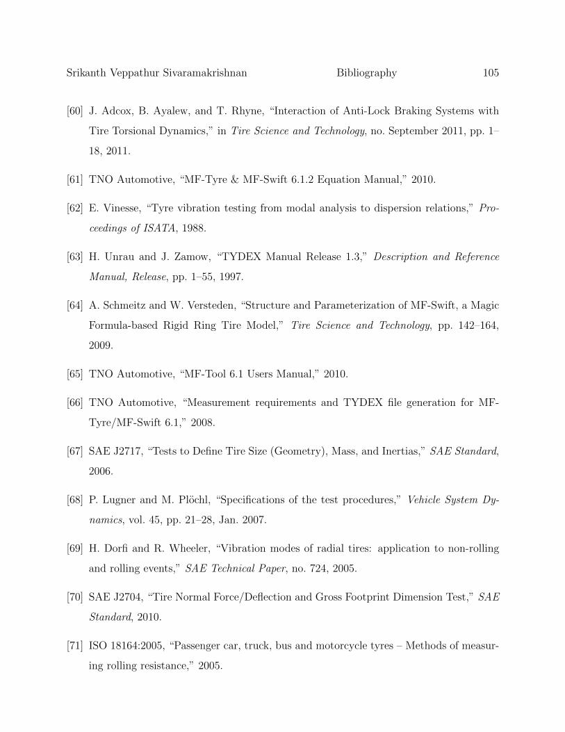
Srikanth Veppathur Sivaramakrishnan Bibliography 105
[60] J. Adcox, B. Ayalew, and T. Rhyne, “Interaction of Anti-Lock Braking Systems with
Tire Torsional Dynamics,” in Tire Science and Technology, no. September 2011, pp. 1–
18, 2011.
[61] TNO Automotive, “MF-Tyre & MF-Swift 6.1.2 Equation Manual,” 2010.
[62] E. Vinesse, “Tyre vibration testing from modal analysis to dispersion relations,” Pro-
ceedings of ISATA, 1988.
[63] H. Unrau and J. Zamow, “TYDEX Manual Release 1.3,” Description and Reference
Manual, Release, pp. 1–55, 1997.
[64] A. Schmeitz and W. Versteden, “Structure and Parameterization of MF-Swift, a Magic
Formula-based Rigid Ring Tire Model,” Tire Science and Technology, pp. 142–164,
2009.
[65] TNO Automotive, “MF-Tool 6.1 Users Manual,” 2010.
[66] TNO Automotive, “Measurement requirements and TYDEX file generation for MF-
Tyre/MF-Swift 6.1,” 2008.
[67] SAE J2717, “Tests to Define Tire Size (Geometry), Mass, and Inertias,” SAE Standard,
2006.
[68] P. Lugner and M. Plochl, “Specifications of the test procedures,” Vehicle System Dy-
namics, vol. 45, pp. 21–28, Jan. 2007.
[69] H. Dorfi and R. Wheeler, “Vibration modes of radial tires: application to non-rolling
and rolling events,” SAE Technical Paper, no. 724, 2005.
[70] SAE J2704, “Tire Normal Force/Deflection and Gross Footprint Dimension Test,” SAE
Standard, 2010.
[71] ISO 18164:2005, “Passenger car, truck, bus and motorcycle tyres – Methods of measur-
ing rolling resistance,” 2005.

Srikanth Veppathur Sivaramakrishnan Bibliography 106
[72] N. Balaramakrishna and R. K. Kumar, “A study on the estimation of SWIFT model
parameters by finite element analysis,” Proceedings of the Institution of Mechanical
Engineers, Part D: Journal of Automobile Engineering, vol. 223, pp. 1283–1300, Oct.
2009.
[73] A. Tuononen, L. Hartikainen, F. Petry, and S. Westermann, “Parameterization of in-
plane rigid ring tire model from instrumented vehicle measurements,” in 11th Interna-
tional Symposium on Advanced Vehicle Control, 2012.
[74] SAE J2730, “Dynamic Cleat Test with Perpendicular and Inclined Cleats,” SAE Stan-
dard, 2006.
[75] SAE J2909, “Light Vehicle Dry Stopping Distance,” SAE Standard, 2010.
[76] G. E. Elkins, P. Schmalzer, T. Thompson, and A. Simpson, “Long-Term Pavement
Performance Information Management System Pavement Performance Database User
Reference Guide,” McLean: Federal Highway Administration, 2003.
[77] TNO Automotive, “MF-Tyre/MF-Swift 6.1.2.1 Help Manual,” 2012.
[78] F. Mancosu, R. Sangalli, F. Cheli, G. Ciarlariello, and F. Braghin, “A Mathematical-
Physical 3D Tire Model for Handling/Comfort Optimization on a Vehicle: Comparison
with Experimental Results,” Tire Science and Technology, vol. 28, pp. 210–232, Oct.
2000.