discrete time signals and systems time-frequency … analysis fourier transform (1d and 2d)...
TRANSCRIPT
Discrete Time Signals and SystemsTime-frequency Analysis
Gloria Menegaz
Time-frequency Analysis
• Fourier transform (1D and 2D)
• Reference textbook:
Discrete time signal processing, A.W. Oppenheim and R.W. Shafer
– Chapter 1: Introduction
– Chapter 2: Discrete time Signals and Systems
– Chapter 3: Sampling of Continuos Time Signals
– (Chapter 4: The z-Transform)
Gloria Menegaz Discrete Time Signals and SystemsTime-frequency Analysis 2
Signal Classification• Continuous time signals x(t) are functions of a continuous indepen-
dent variable tx = x(t), t ∈ R
• Discrete time signals are functions of a discrete variablex = {x[n]},n ∈ Z,−∞ < n <+∞
– Are defined at discrete time intervals
– Are represented as sequences of numbers
• Digital signals both the independent variable and the amplitude arediscrete
Digital systems: both the input and the output are digital signals⇒ Digital Signal Processing: processing of signals that are discrete in bothtime and amplitude
Gloria Menegaz Discrete Time Signals and SystemsTime-frequency Analysis 3
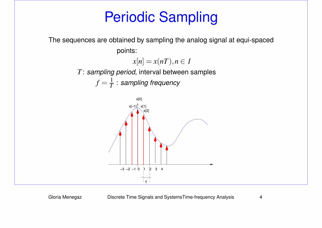
Periodic SamplingThe sequences are obtained by sampling the analog signal at equi-spaced
points:
x[n] = x(nT ),n ∈ IT : sampling period, interval between samples
f = 1T : sampling frequency
1 2 3 4−1−2−3 0
x[0]
x[−1] x[1]x[2]
T
Gloria Menegaz Discrete Time Signals and SystemsTime-frequency Analysis 4

Basic Sequences
• Products and sums among sequences: element by element operations
• Delayed or shifted sequence: y[n] = x[n− k]
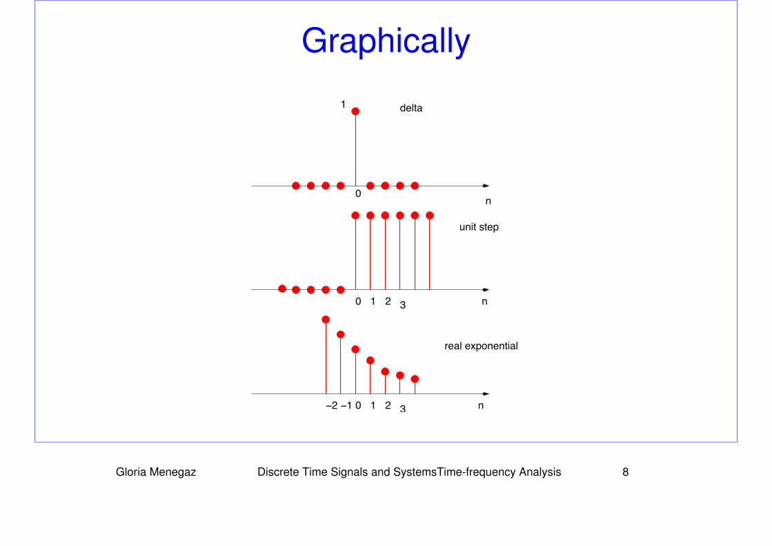
• Unit sample sequence δ[n] (Dirac function, impulse):
δ[n] =
{0, n 6= 01, n = 0
(1)
• Unit step sequence:
u[n] =
{0, n < 01, n≥ 0
(2)
Gloria Menegaz Discrete Time Signals and SystemsTime-frequency Analysis 5
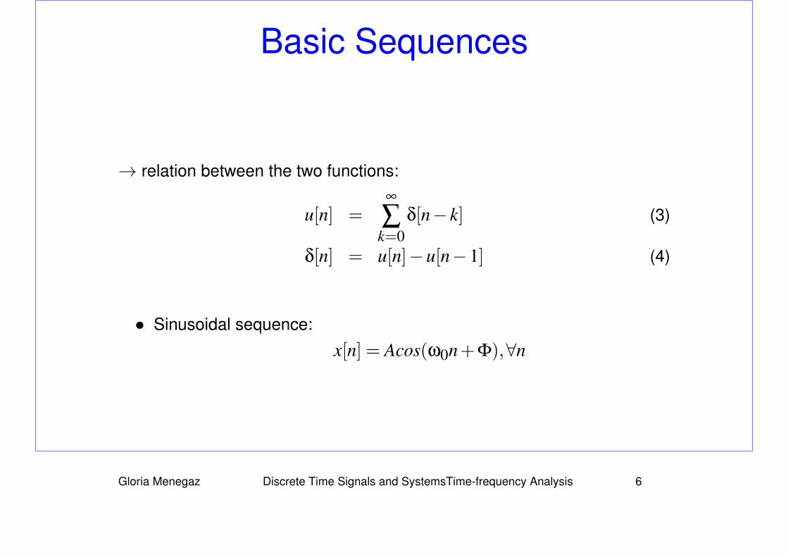
Basic Sequences
→ relation between the two functions:
u[n] =∞
∑k=0
δ[n− k] (3)
δ[n] = u[n]−u[n−1] (4)
• Sinusoidal sequence:
x[n] = Acos(ω0n+Φ),∀n
Gloria Menegaz Discrete Time Signals and SystemsTime-frequency Analysis 6
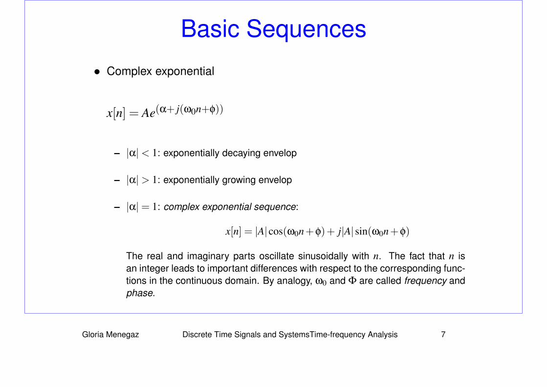
Basic Sequences
• Complex exponential
x[n] = Ae(α+ j(ω0n+φ))
– |α|< 1: exponentially decaying envelop
– |α|> 1: exponentially growing envelop
– |α|= 1: complex exponential sequence:
x[n] = |A|cos(ω0n+φ)+ j|A|sin(ω0n+φ)
The real and imaginary parts oscillate sinusoidally with n. The fact that n isan integer leads to important differences with respect to the corresponding func-tions in the continuous domain. By analogy, ω0 and Φ are called frequency andphase.
Gloria Menegaz Discrete Time Signals and SystemsTime-frequency Analysis 7
Graphically
n
n
n
1
0
0 1 2 3
0−1−2 1 2 3
delta
unit step
real exponential
Gloria Menegaz Discrete Time Signals and SystemsTime-frequency Analysis 8
Discrete vs. continuous1. Complex exponentials and sinusoids are 2π-periodic
x[n] = Aexp j(ω0+2π)n = Aexp jω0n exp j2πn = Aexp jω0n (5)
⇒ Complex exponentials with frequencies (ω0 + 2πr) are indistin-guishable from one another⇒ only frequencies in an interval of length2π need to be considered
2. Complex exponentials in general are not periodicPeriodicity condition: x[n] = x[n+N], ∀n,N ∈ I. For this condition tobe true, the following relation must hold true:
ω0N = 2πk, k ∈ I (6)
⇒ Complex exponentials and sinusoidal sequences are not necessar-ily periodic with period T0 = 2π/ω0 as in the continuous domain and,depending on the value of ω0, might not be periodic at all.
Gloria Menegaz Discrete Time Signals and SystemsTime-frequency Analysis 9
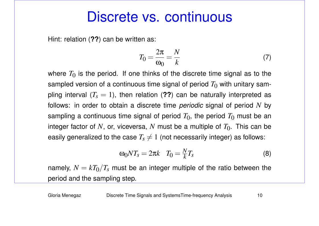
Discrete vs. continuousHint: relation (??) can be written as:
T0 =2π
ω0=
Nk
(7)
where T0 is the period. If one thinks of the discrete time signal as to the
sampled version of a continuous time signal of period T0 with unitary sam-
pling interval (Ts = 1), then relation (??) can be naturally interpreted as
follows: in order to obtain a discrete time periodic signal of period N by
sampling a continuous time signal of period T0, the period T0 must be an
integer factor of N, or, viceversa, N must be a multiple of T0. This can be
easily generalized to the case Ts 6= 1 (not necessarily integer) as follows:
ω0NTs = 2πk T0 =Nk Ts (8)
namely, N = kT0/Ts must be an integer multiple of the ratio between the
period and the sampling step.
Gloria Menegaz Discrete Time Signals and SystemsTime-frequency Analysis 10
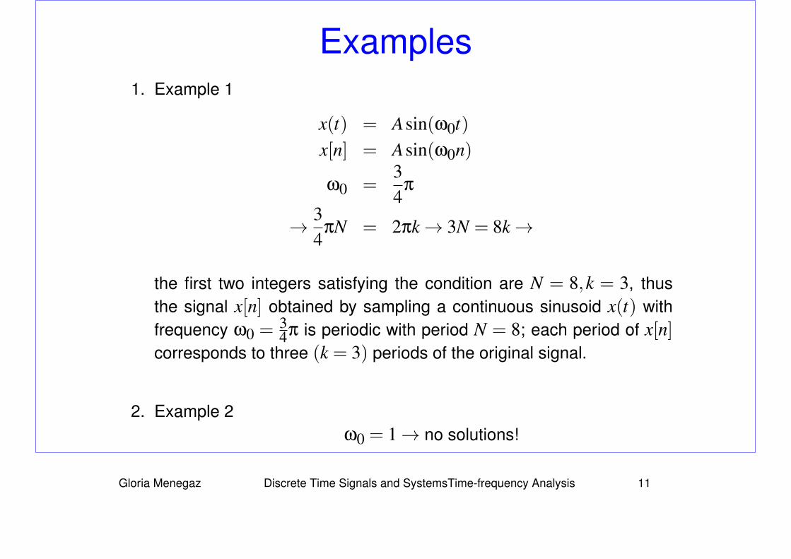
Examples1. Example 1
x(t) = Asin(ω0t)x[n] = Asin(ω0n)
ω0 =34
π
→ 34
πN = 2πk→ 3N = 8k→
the first two integers satisfying the condition are N = 8,k = 3, thusthe signal x[n] obtained by sampling a continuous sinusoid x(t) withfrequency ω0 = 3
4π is periodic with period N = 8; each period of x[n]corresponds to three (k = 3) periods of the original signal.
2. Example 2ω0 = 1→ no solutions!
Gloria Menegaz Discrete Time Signals and SystemsTime-frequency Analysis 11
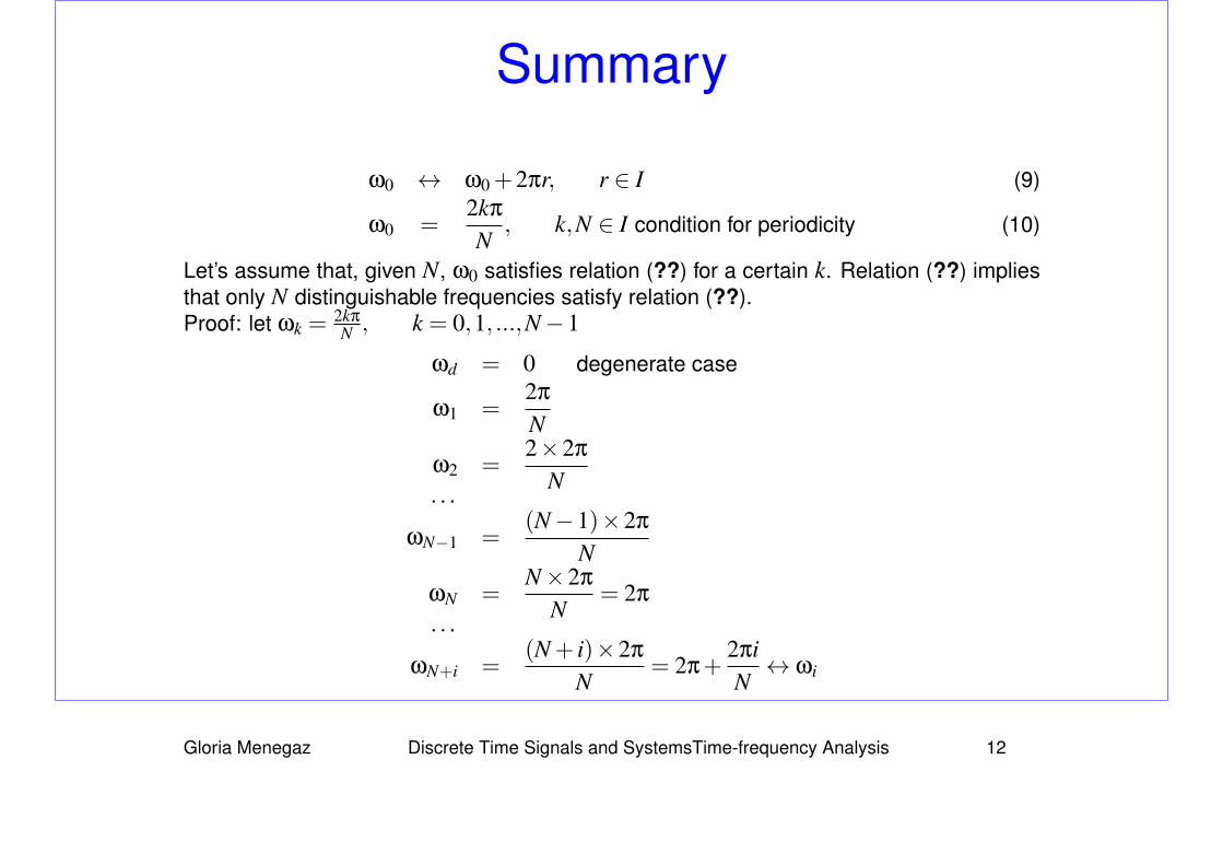
Summary
ω0 ↔ ω0+2πr, r ∈ I (9)
ω0 =2kπ
N, k,N ∈ I condition for periodicity (10)
Let’s assume that, given N, ω0 satisfies relation (??) for a certain k. Relation (??) impliesthat only N distinguishable frequencies satisfy relation (??).Proof: let ωk =
2kπ
N , k = 0,1, ...,N−1
ωd = 0 degenerate case
ω1 =2π
N
ω2 =2×2π
N. . .
ωN−1 =(N−1)×2π
N
ωN =N×2π
N= 2π
. . .
ωN+i =(N + i)×2π
N= 2π+
2πiN↔ ωi
Gloria Menegaz Discrete Time Signals and SystemsTime-frequency Analysis 12
Examples
Gloria Menegaz Discrete Time Signals and SystemsTime-frequency Analysis 13
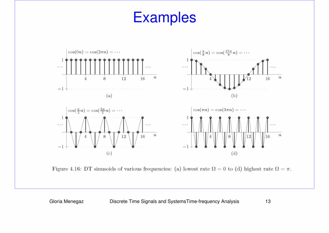
Discrete vs Continuous
Conclusion: for a sinusoidal signal x[n] = Asin(ω0n), as ω0 increases from
ω0 = 0 to ω0 = π, x[n] oscillates more and more rapidly. Conversely, from
ω0 = π to ω0 = 2π the oscillations become slower. In fact, because of
the periodicity in ω0 of complex exponentials and sinusoidal sequences,
ω0 = 0 is indistinguishable from ω0 = 2π and, more in general, frequencies
around ω0 = 2π are indistinguishable from frequencies around ω0 = 0. As
a consequence, values of ω0 in the vicinity of ω0 = 2kπ are referred to as
low frequencies, whereas frequencies in the vicinity of ω0 = (2k+1)π are
referred to as high frequencies. This is a fundamental difference from the
continuous case, where the speed of the oscillations increases monotoni-
cally with the frequency ω0.
Gloria Menegaz Discrete Time Signals and SystemsTime-frequency Analysis 14
Operations and Properties
• Periodicity: a sequence is periodic with period N iif:
x[n+N] = x[n],∀n
• Energy: E = ∑+∞n=−∞ |x[n]|2
• Sample-wise operations:
– Product: x · y = {x[n]y[n]}
– Sum: x+ y = {x[n]+ y[n]}
– Scaling: αx = {αx[n]}
– Delay: y[n] = x[n−n0],n,n0 ∈ I
Gloria Menegaz Discrete Time Signals and SystemsTime-frequency Analysis 15
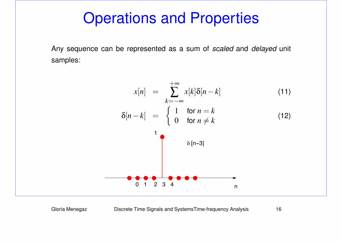
Operations and Properties
Any sequence can be represented as a sum of scaled and delayed unit
samples:
x[n] =+∞
∑k=−∞
x[k]δ[n− k] (11)
δ[n− k] =
{1 for n = k0 for n 6= k
(12)
n
1
3 4210
b [n−3]
Gloria Menegaz Discrete Time Signals and SystemsTime-frequency Analysis 16
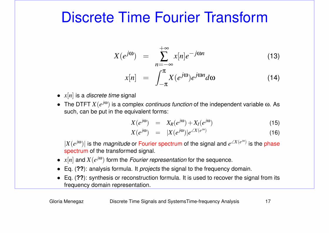
Discrete Time Fourier Transform
X(e jω) =+∞
∑n=−∞
x[n]e− jωn (13)
x[n] =∫
π
−π
X(e jω)e jωndω (14)
• x[n] is a discrete time signal• The DTFT X(e jω) is a complex continuos function of the independent variable ω. As
such, can be put in the equivalent forms:
X(e jω) = XR(e jω)+XI(e jω) (15)
X(e jω) = |X(e jω)|e∠X(e jω) (16)
|X(e jω)| is the magnitude or Fourier spectrum of the signal and e∠X(e jω) is the phasespectrum of the transformed signal.
• x[n] and X(e jω) form the Fourier representation for the sequence.• Eq. (??): analysis formula. It projects the signal to the frequency domain.• Eq. (??): synthesis or reconstruction formula. It is used to recover the signal from its
frequency domain representation.
Gloria Menegaz Discrete Time Signals and SystemsTime-frequency Analysis 17
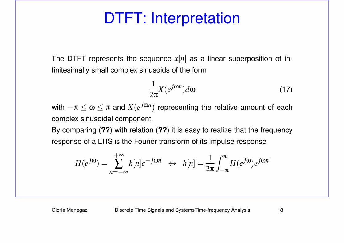
DTFT: Interpretation
The DTFT represents the sequence x[n] as a linear superposition of in-
finitesimally small complex sinusoids of the form
12π
X(e jωn)dω (17)
with −π ≤ ω ≤ π and X(e jωn) representing the relative amount of each
complex sinusoidal component.
By comparing (??) with relation (??) it is easy to realize that the frequency
response of a LTIS is the Fourier transform of its impulse response
H(e jω) =+∞
∑n=−∞
h[n]e− jωn ↔ h[n] =1
2π
∫π
−π
H(e jω)e jωn
Gloria Menegaz Discrete Time Signals and SystemsTime-frequency Analysis 18
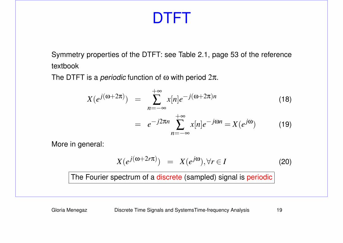
DTFT
Symmetry properties of the DTFT: see Table 2.1, page 53 of the reference
textbook
The DTFT is a periodic function of ω with period 2π.
X(e j(ω+2π)) =+∞
∑n=−∞
x[n]e− j(ω+2π)n (18)
= e− j2πn+∞
∑n=−∞
x[n]e− jωn = X(e jω) (19)
More in general:
X(e j(ω+2rπ)) = X(e jω),∀r ∈ I (20)
The Fourier spectrum of a discrete (sampled) signal is periodic
Gloria Menegaz Discrete Time Signals and SystemsTime-frequency Analysis 19
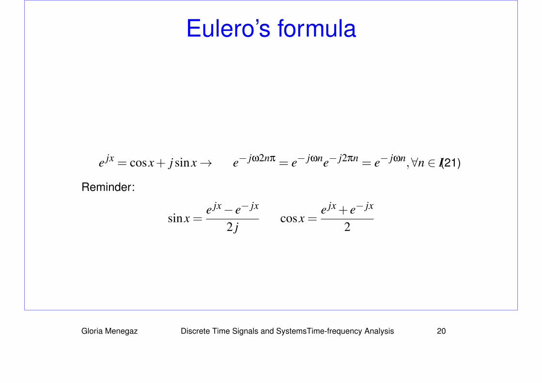
Eulero’s formula
e jx = cosx+ j sinx→ e− jω2nπ = e− jωne− j2πn = e− jωn,∀n ∈ I(21)
Reminder:
sinx =e jx− e− jx
2 jcosx =
e jx+ e− jx
2
Gloria Menegaz Discrete Time Signals and SystemsTime-frequency Analysis 20
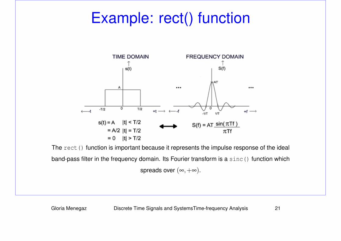
Example: rect() function
The rect() function is important because it represents the impulse response of the ideal
band-pass filter in the frequency domain. Its Fourier transform is a sinc() function which
spreads over (∞,+∞).
Gloria Menegaz Discrete Time Signals and SystemsTime-frequency Analysis 21
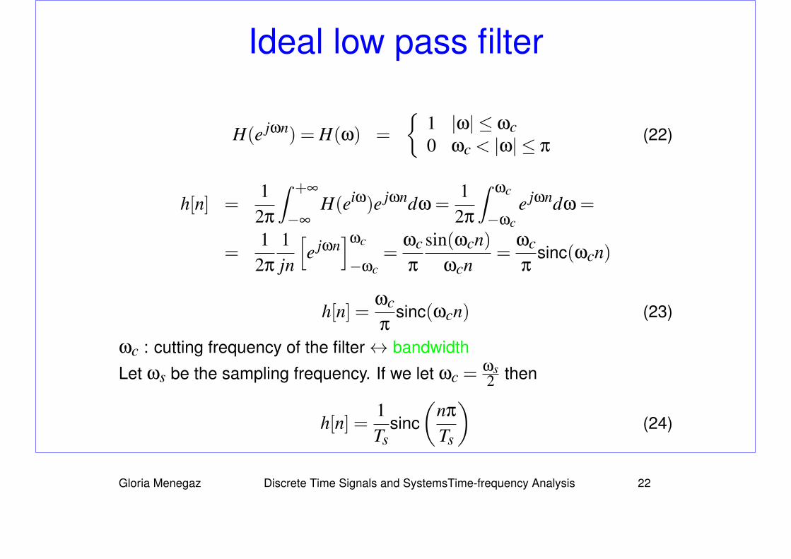
Ideal low pass filter
H(e jωn) = H(ω) =
{1 |ω| ≤ ωc0 ωc < |ω| ≤ π
(22)
h[n] =1
2π
∫ +∞
−∞
H(eiω)e jωndω =1
2π
∫ωc
−ωce jωndω =
=1
2π
1jn
[e jωn
]ωc
−ωc=
ωcπ
sin(ωcn)ωcn
=ωcπ
sinc(ωcn)
h[n] =ωcπ
sinc(ωcn) (23)
ωc : cutting frequency of the filter↔ bandwidth
Let ωs be the sampling frequency. If we let ωc =ωs2 then
h[n] =1Ts
sinc
(nπ
Ts
)(24)
Gloria Menegaz Discrete Time Signals and SystemsTime-frequency Analysis 22
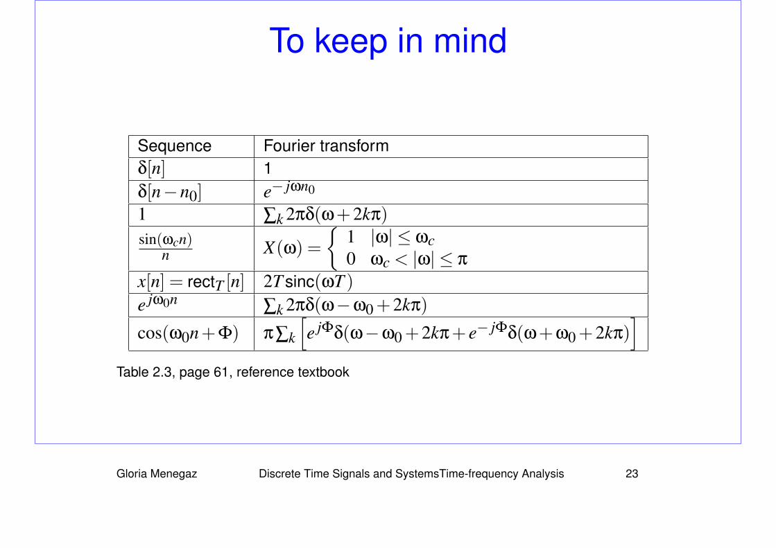
To keep in mind
Sequence Fourier transformδ[n] 1δ[n−n0] e− jωn0
1 ∑k 2πδ(ω+2kπ)
sin(ωcn)n X(ω) =
{1 |ω| ≤ ωc0 ωc < |ω| ≤ π
x[n] = rectT [n] 2T sinc(ωT )e jω0n
∑k 2πδ(ω−ω0+2kπ)
cos(ω0n+Φ) π∑k
[e jΦδ(ω−ω0+2kπ+ e− jΦδ(ω+ω0+2kπ)
]Table 2.3, page 61, reference textbook
Gloria Menegaz Discrete Time Signals and SystemsTime-frequency Analysis 23
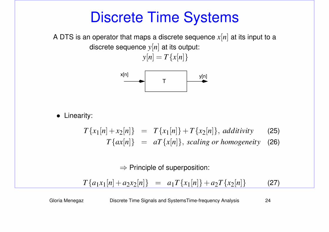
Discrete Time SystemsA DTS is an operator that maps a discrete sequence x[n] at its input to a
discrete sequence y[n] at its output:y[n] = T{x[n]}
Tx[n] y[n]
• Linearity:
T{x1[n]+ x2[n]} = T{x1[n]}+T{x2[n]}, additivity (25)
T{ax[n]} = aT{x[n]}, scaling or homogeneity (26)
⇒ Principle of superposition:
T{a1x1[n]+a2x2[n]} = a1T{x1[n]}+a2T{x2[n]} (27)
Gloria Menegaz Discrete Time Signals and SystemsTime-frequency Analysis 24
Discrete Time Systems
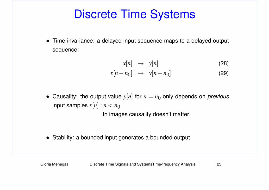
• Time-invariance: a delayed input sequence maps to a delayed output
sequence:
x[n] → y[n] (28)
x[n−n0] → y[n−n0] (29)
• Causality: the output value y[n] for n = n0 only depends on previous
input samples x[n] : n < n0In images causality doesn’t matter!
• Stability: a bounded input generates a bounded output
Gloria Menegaz Discrete Time Signals and SystemsTime-frequency Analysis 25
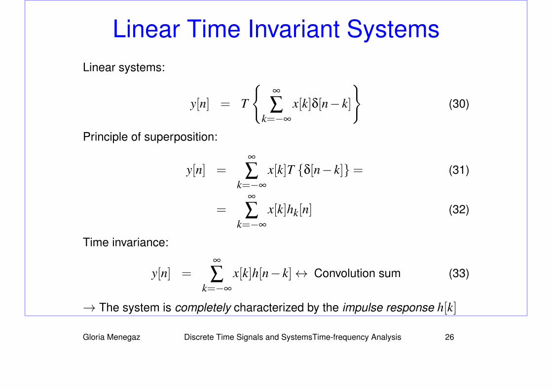
Linear Time Invariant SystemsLinear systems:
y[n] = T
{∞
∑k=−∞
x[k]δ[n− k]
}(30)
Principle of superposition:
y[n] =∞
∑k=−∞
x[k]T {δ[n− k]}= (31)
=∞
∑k=−∞
x[k]hk[n] (32)
Time invariance:
y[n] =∞
∑k=−∞
x[k]h[n− k]↔ Convolution sum (33)
→ The system is completely characterized by the impulse response h[k]
Gloria Menegaz Discrete Time Signals and SystemsTime-frequency Analysis 26

Convolution operator
x[n]? y[n] =+∞
∑k=−∞
x[k] · y[n− k] (34)
=+∞
∑k=−∞
x[n− k] · y[k] (35)
Recipe for the convolution (refer to( ??)):1. Reflect y[k] about the origin to get y[−k]
2. Shift the reflected sequence of n steps
3. Multiply (point wise) the resulting sequence by x[n]
4. Sum over the samples of the resulting signal to get the value of the convolution atposition n
5. Increment n and ge back to point 2.
Gloria Menegaz Discrete Time Signals and SystemsTime-frequency Analysis 27
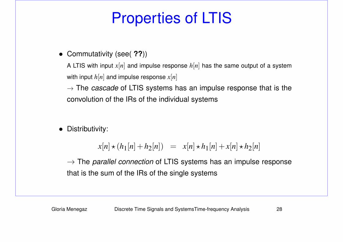
Properties of LTIS
• Commutativity (see( ??))
A LTIS with input x[n] and impulse response h[n] has the same output of a system
with input h[n] and impulse response x[n]
→ The cascade of LTIS systems has an impulse response that is the
convolution of the IRs of the individual systems
• Distributivity:
x[n]? (h1[n]+h2[n]) = x[n]?h1[n]+ x[n]?h2[n]
→ The parallel connection of LTIS systems has an impulse response
that is the sum of the IRs of the single systems
Gloria Menegaz Discrete Time Signals and SystemsTime-frequency Analysis 28
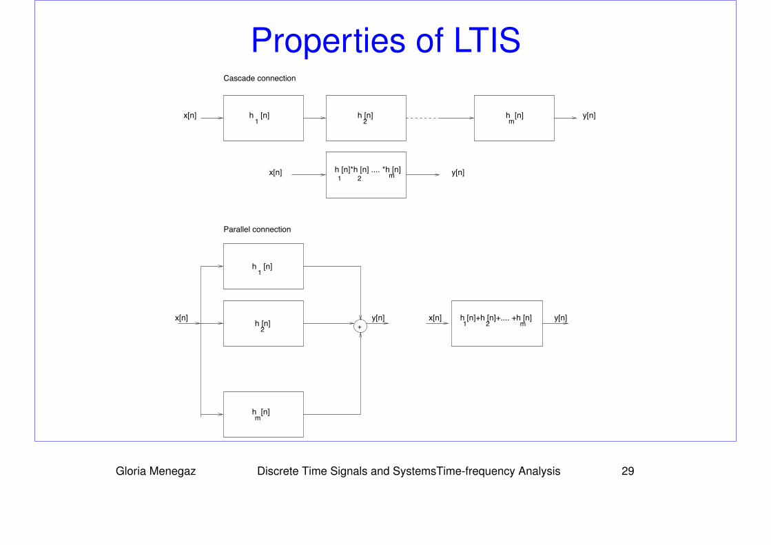
Properties of LTIS
h1
[n]
h [n]2
h [n]m
h [n]+h [n]+.... +h [n]1 2 m+
h [n]*h [n] .... *h [n]1 2 m
h1
[n] h [n]2
h [n]m
Cascade connection
Parallel connection
x[n] y[n]
x[n] y[n]
x[n] y[n] x[n] y[n]
Gloria Menegaz Discrete Time Signals and SystemsTime-frequency Analysis 29
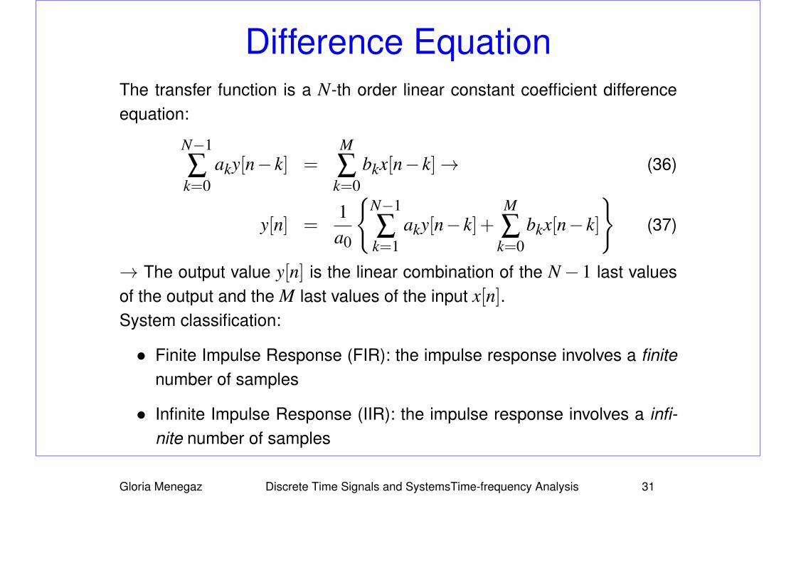
Difference EquationThe transfer function is a N-th order linear constant coefficient differenceequation:
N−1
∑k=0
aky[n− k] =M
∑k=0
bkx[n− k]→ (36)
y[n] =1a0
{N−1
∑k=1
aky[n− k]+M
∑k=0
bkx[n− k]
}(37)
→ The output value y[n] is the linear combination of the N− 1 last valuesof the output and the M last values of the input x[n].System classification:
• Finite Impulse Response (FIR): the impulse response involves a finitenumber of samples
• Infinite Impulse Response (IIR): the impulse response involves a infi-nite number of samples
Gloria Menegaz Discrete Time Signals and SystemsTime-frequency Analysis 31
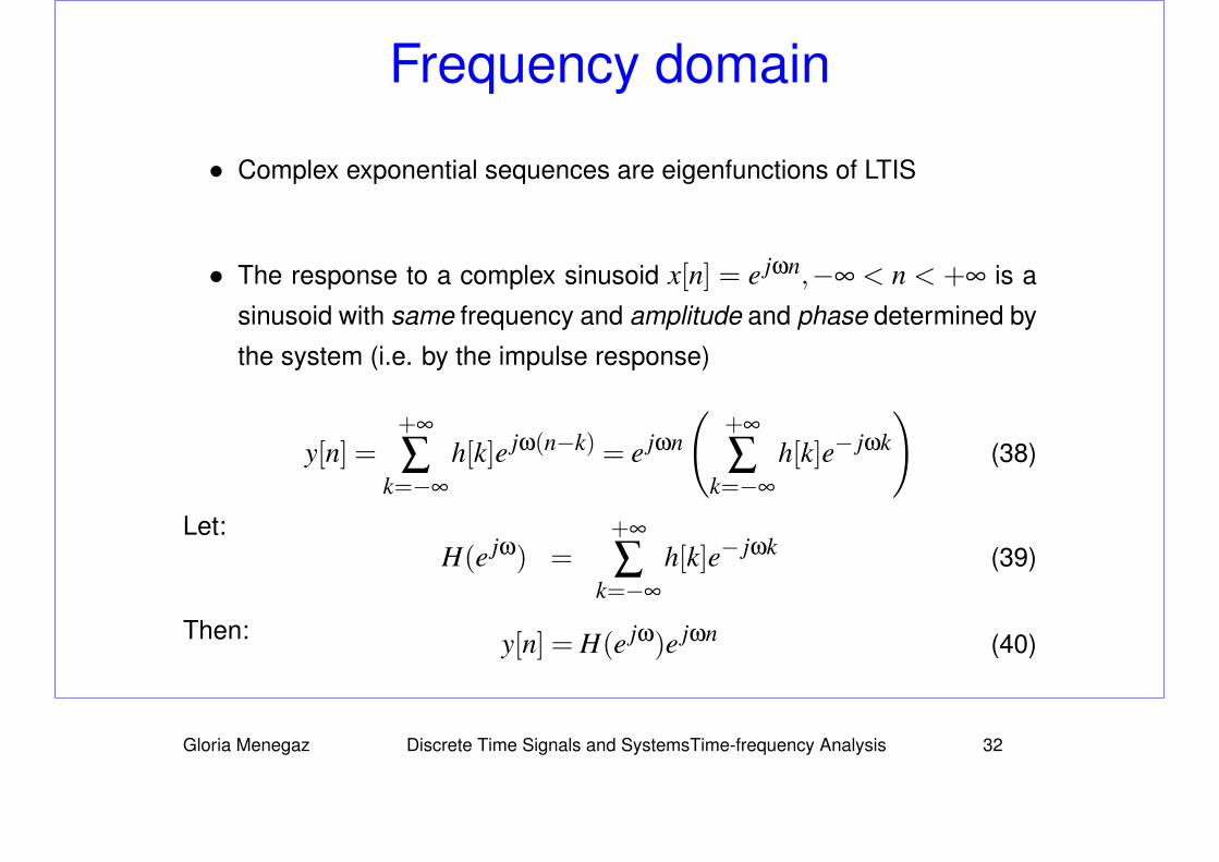
Frequency domain
• Complex exponential sequences are eigenfunctions of LTIS
• The response to a complex sinusoid x[n] = e jωn,−∞ < n < +∞ is a
sinusoid with same frequency and amplitude and phase determined by
the system (i.e. by the impulse response)
y[n] =+∞
∑k=−∞
h[k]e jω(n−k) = e jωn
(+∞
∑k=−∞
h[k]e− jωk
)(38)
Let:H(e jω) =
+∞
∑k=−∞
h[k]e− jωk (39)
Then: y[n] = H(e jω)e jωn (40)
Gloria Menegaz Discrete Time Signals and SystemsTime-frequency Analysis 32
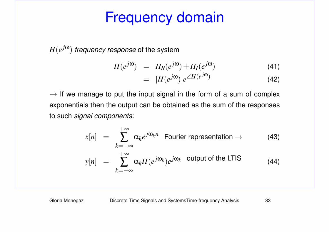
Frequency domain
H(e jω) frequency response of the system
H(e jω) = HR(ejω)+HI(e
jω) (41)
= |H(e jω)|e∠H(e jω) (42)
→ If we manage to put the input signal in the form of a sum of complex
exponentials then the output can be obtained as the sum of the responses
to such signal components:
x[n] =+∞
∑k=−∞
αke jωkn Fourier representation→ (43)
y[n] =+∞
∑k=−∞
αkH(e jωk)e jωk output of the LTIS (44)
Gloria Menegaz Discrete Time Signals and SystemsTime-frequency Analysis 33
Frequency response of a LTIS
H(e jω) is always a periodic function of ω with period 2π
H(e j(ω+2rπ)) =+∞
∑n=−∞
h[n]e− j(ω+2rπ)n =+∞
∑n=−∞
h[n]e− jωn = H(e jω)
(45)
Due to this property as well as to the fact that frequencies differing for mul-
tiples of 2π are indistinguishable, H(e jω) only needs to be specified over
an interval of length 2π. The inherent periodicity defines the frequency re-
sponse on the entire frequency axis. It is common use to specify H over
the interval −π ≤ ω ≤ π. Then, the frequencies around even multiples of
π are referred to as low frequencies, while those around odd multiples of π
are high frequencies.
Gloria Menegaz Discrete Time Signals and SystemsTime-frequency Analysis 34