discrete-time markov chain (dtmc) state space distribution · continuous-time markov models single...

1

Discrete-time Markov chain (DTMC)

State space distribution

pi(t) = P{Xt = i}

Transient solution: p(t)

State occupancy vector at time t in terms of the transition probability matrix:

p(t) = p(0) Pt

Probability that the Markov process is in state i at time-step t

System evolution in a finite number of steps computed starting from the

initial state distribution and the transition probability matrix

= (p1 , …, pn ) p(0) (0) (0)

p(t) = [p0(t), p1

(t), p2(t) , …] state occupancy vector at time t

p(1) = p(0) P

initial state space distribution:

A single step forward:

2

Limiting behaviour

A Markov process can be specified in terms of the state occupancy

probability vector p and a transition probability matrix P

p(t) = p(0) Pt

The limiting behaviour of a DTMC depends on the

characteristics of its states. Sometimes the solution is simple.

The limiting behaviour of a DTMC (steady-state behaviour):

3

Irreducible DTMC

A state j is said to be accessible from state i if there exists t >0

such that Pij(t) >0, we write i->j

A DTMC is irreducible if each state is accessible from every

other state in a finite number of steps :

for each i, j: i -> j

A subset S’ of S is closed if there not exists any transition

from S’ to S-S’

4

Classification of states

A state i is recurrent if

(i->j) then (j->i)

process moves again to state i with probability 1

recurrent non-null: medium time of recurrence is finite

recurrent null: medium time of recurrence is infinite

A state i is transient if

exists (j!=i) such that (i->j) and not (j->i)

A state i is absorbent if

pii=1

(i is a recurrent state)

5

Classification of states Given a recurrent state, let d be the greatest common divisor of

all the integers m such that Pii(m) > 0

A recurrent state i is periodic if d > 1

A recurrent state i is aperiodic if d = 1: it is possible to move to

the same state in one step

1 2

state 1 is periodic with period d=2

state 2 is periodic with period d=2

1

1

6

Steady-state behaviour

Moreover, if all states are recurrent non-null, the steady-

state behaviour of the Markov chain is given by the fixpoint of

the equation:

p(t) = p(t-1) P with

Sj pj =1

THEOREM:

For aperiodic irreducible Markov chain for each j

exists and the solution is independent from p(0)

pj is inversely proportional to the period of recurrence of state j

7

Time-average state space distribution

For periodic Markov chains

doesn’t exist (caused by the

probability of the periodic state)

We compute the time-average

state space distribution, called p*

1 2

1 0 1

2 1 0

p(0) = (1,0)

p(1) = p(0) P p(1) = (0,1)

p(2) = p(1) P p(2) = (1,0)

………..

P=

1 2

p(0) =(1,0)

p* = state i is periodic with period d=2

1

1

9

Continuous-time models:

state transitions occur at random intervals

transition rates assigned to each transition

Markov property assumption:

the length of time already spent in a state does not influence either the

probability distribution of the next state or the probability distribution of

remaining time in the same state before the next transition

These very strong assumptions imply that the waiting time spent in any

one state is exponentially distributed

Thus the Markov model naturally fits with the standard assumptions that

failure rates are constant, leading to exponential distribution of

interarrivals of failures

Continuous-time Markov models

10


Single system with repair

failure rate, m repair rate state 0: working

state 1: failed

p0(t) probability of being in the operational state

p1(t) probability of being in the failed state

Graph model

Transition Matrix P

derived from the discrete time model, taking the limit as

the time-step interval approaches zero

11

Probability of being in state 0 or 1 at time t+Dt:


Performing multiplication, rearranging and dividing by Dt, taking the limit as

Dt approaches to 0:

probability of being in

state 0 at time t+Dt

Continuous-time Chapman-Kolmogorov equations

12

Matrix form:


The set of equations can be written by inspection of a transition diagram

without self-loops and Dt’s:

T matrix

Continuous time Markov model graph

The change in state 0 is minus the flow out of state 0 times the probability

of being in state 0 at time t, plus the flow into state 0 from state 1 times

the probability of being in state 1.

13

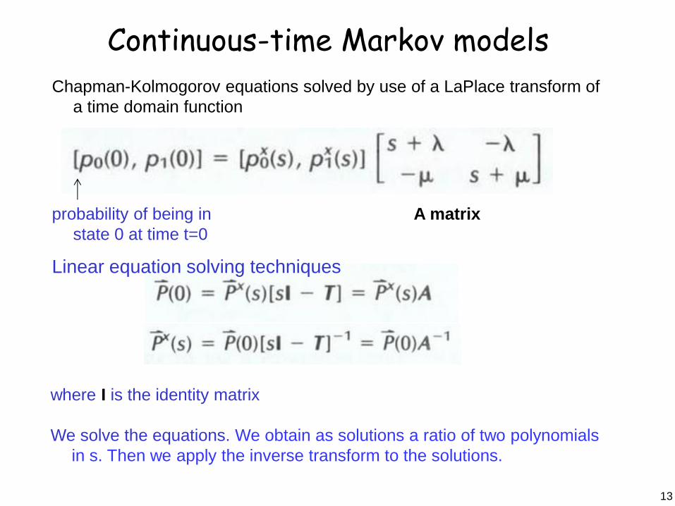
Chapman-Kolmogorov equations solved by use of a LaPlace transform of

a time domain function


where I is the identity matrix

We solve the equations. We obtain as solutions a ratio of two polynomials

in s. Then we apply the inverse transform to the solutions.

probability of being in

state 0 at time t=0

A matrix

Linear equation solving techniques

14


Assume the system starts in the operational state: P(0) = [1,0]

We apply the inverse transforms.

Our example

15


p0(t) probability that the system is in the operational state at time t,

availability at time t

The availability consists of a steady-state term and an exponential

decaying transient term

A(t)

Only steady-state solution

Chapman-Kolmogorov equations: derivative replaced by 0; p0(t) replaced by p0(0) and p1(t)

replaced by p1(0)

16

Availability as a function of time

= 0.001

m = 0.1

The steady-state

value is reached in

a very short time

17

Markov model making the system-failed state

a trapping state

Continuous-time Markov models: Reliability

Differential equations:

Single system without repair

T matrix

Continuous time Markov model graph

Dt = state transition probability

= failure rate

T matrix can be built by

inspection

18

Taking the inverse transform:

A matrix

A= [sI –T]

Continuous-time Markov models: Reliability

Continuous-time homogeneous Markov chains (CTMC)

19

X random process that represents the number of operational memories and the

number of operational processors at time t

Given a state (i, j):

i is the number of operational memories;

j is the number of operational processors

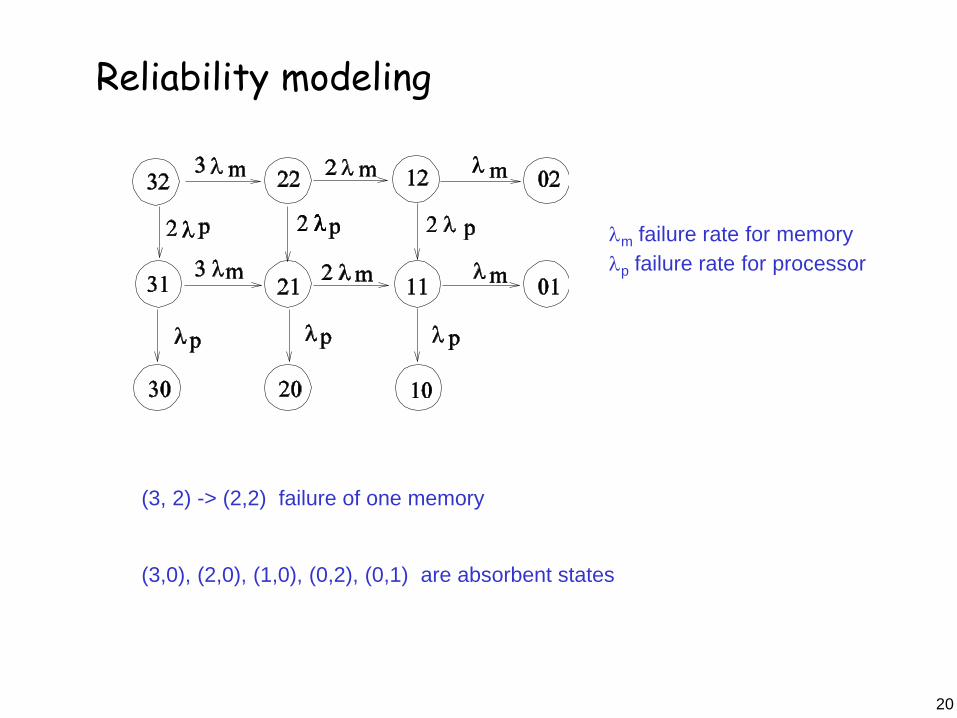
An example of modeling (CTMC)

m failure rate for memory

p failure rate for processor

Multiprocessor system with 2 processors and 3 shared memories system.

System is operational if at least one processor and one memory are

operational.

S = {(3,2), (3,1), (3,0), (2,2), (2,1), (2,0), (1,2), (1,1), (1,0), (0,2), (0,1)}

20

(3, 2) -> (2,2) failure of one memory

(3,0), (2,0), (1,0), (0,2), (0,1) are absorbent states



Reliability modeling

21

Assume that faulty components are replaced and we evaluate the

probability that the system is operational at time t

Constant repair rate m (number of expected repairs in a unit of time)

Strategy of repair:

only one processor or one memory at a time can be substituted

The behaviour of components (with respect of being operational or failed)

is not independent: it depends on whether or not other components are

in a failure state.

Availability modeling

22

Strategy of repair:

only one component can be substituted at a time



mm repair rate for memory

mp repair rate for processor

23

An alternative strategy of repair:

only one component can be substituted at a time and processors have

higher priority

exclude the lines mm representing memory repair in the case where there

has been a process failure

discrete-time markov chain (dtmc) state space distribution · continuous-time markov models single...

Documents