discrete mathematics and algebra - university of london

Discrete mathematics and algebraR. SimonMT3170, 2790170

2011

Undergraduate study in Economics, Management, Finance and the Social Sciences

This is an extract from a subject guide for an undergraduate course offered as part of the University of London International Programmes in Economics, Management, Finance and the Social Sciences. Materials for these programmes are developed by academics at the London School of Economics and Political Science (LSE).

For more information, see: www.londoninternational.ac.uk

This guide was prepared for the University of London International Programmes by:

Dr R.Simon, Lecturer, Department of Mathematics, London School of Economics and Political Science.

This is one of a series of subject guides published by the University. We regret that due to pressure of work the author is unable to enter into any correspondence relating to, or arising from, the guide. If you have any comments on this subject guide, favourable or unfavourable, please use the form at the back of this guide.

University of London International Programmes

Publications OfficeStewart House32 Russell SquareLondon WC1B 5DNUnited Kingdom

Website: www.londoninternational.ac.uk

Published by: University of London

© University of London 2011

The University of London asserts copyright over all material in this subject guide except where otherwise indicated. All rights reserved. No part of this work may be reproduced in any form, or by any means, without permission in writing from the publisher.

We make every effort to contact copyright holders. If you think we have inadvertently used your copyright material, please let us know.

Contents

Contents

1 Introduction 1

1.1 This course . . . . . . . . . . . . . . . . . . . . . . . . . . . . . . . . . . 1

1.1.1 Relationship to previous mathematics courses . . . . . . . . . . . 1

1.1.2 Aims . . . . . . . . . . . . . . . . . . . . . . . . . . . . . . . . . . 1

1.1.3 Learning outcomes . . . . . . . . . . . . . . . . . . . . . . . . . . 1

1.1.4 Topics covered . . . . . . . . . . . . . . . . . . . . . . . . . . . . . 2

1.2 Recommended books . . . . . . . . . . . . . . . . . . . . . . . . . . . . . 2

1.2.1 Essential reading . . . . . . . . . . . . . . . . . . . . . . . . . . . 2

1.2.2 Further reading . . . . . . . . . . . . . . . . . . . . . . . . . . . . 3

1.3 Online study resources . . . . . . . . . . . . . . . . . . . . . . . . . . . . 3

1.3.1 The VLE . . . . . . . . . . . . . . . . . . . . . . . . . . . . . . . 4

1.3.2 Making use of the Online Library . . . . . . . . . . . . . . . . . . 4

1.4 Examination advice . . . . . . . . . . . . . . . . . . . . . . . . . . . . . . 5

1.5 Basic notation . . . . . . . . . . . . . . . . . . . . . . . . . . . . . . . . . 6

2 Elementary counting 7

Essential reading . . . . . . . . . . . . . . . . . . . . . . . . . . . . . . . . . . 7

Further reading . . . . . . . . . . . . . . . . . . . . . . . . . . . . . . . . . . . 7

2.1 Introduction . . . . . . . . . . . . . . . . . . . . . . . . . . . . . . . . . . 7

2.2 Selections . . . . . . . . . . . . . . . . . . . . . . . . . . . . . . . . . . . 7

2.2.1 Number of functions . . . . . . . . . . . . . . . . . . . . . . . . . 7

2.2.2 Functions with restrictions and equivalence relations . . . . . . . 8

2.2.3 Pascal’s triangle . . . . . . . . . . . . . . . . . . . . . . . . . . . . 12

Exercises for section 2.2 . . . . . . . . . . . . . . . . . . . . . . . . . . . 14

2.3 Inclusion-exclusion . . . . . . . . . . . . . . . . . . . . . . . . . . . . . . 14

2.3.1 The theorem . . . . . . . . . . . . . . . . . . . . . . . . . . . . . . 15

2.3.2 Applications . . . . . . . . . . . . . . . . . . . . . . . . . . . . . . 17

2.3.3 Surjective functions . . . . . . . . . . . . . . . . . . . . . . . . . . 18


2.4 Partitions and permutations . . . . . . . . . . . . . . . . . . . . . . . . . 23

i

Contents

2.4.1 Partitions of an integer . . . . . . . . . . . . . . . . . . . . . . . . 23

2.4.2 Partition and cycle types . . . . . . . . . . . . . . . . . . . . . . . 23

2.4.3 Number of partitions . . . . . . . . . . . . . . . . . . . . . . . . . 24

2.4.4 Permutations . . . . . . . . . . . . . . . . . . . . . . . . . . . . . 26

2.4.5 Ferrers diagrams . . . . . . . . . . . . . . . . . . . . . . . . . . . 29


2.5 The Stirling numbers . . . . . . . . . . . . . . . . . . . . . . . . . . . . . 31

2.5.1 Stirling numbers of the first kind . . . . . . . . . . . . . . . . . . 31

2.5.2 Stirling numbers of the second kind . . . . . . . . . . . . . . . . . 32

2.5.3 Number of permutations . . . . . . . . . . . . . . . . . . . . . . . 34


Learning outcomes . . . . . . . . . . . . . . . . . . . . . . . . . . . . . . . . . 38

Solutions to exercises . . . . . . . . . . . . . . . . . . . . . . . . . . . . . . . . 38

Solutions to section 2.2 exercises . . . . . . . . . . . . . . . . . . . . . . . 38




3 Generating functions 47


Further reading . . . . . . . . . . . . . . . . . . . . . . . . . . . . . . . . . . . 47

3.1 Introduction . . . . . . . . . . . . . . . . . . . . . . . . . . . . . . . . . . 47

3.2 The basic theory . . . . . . . . . . . . . . . . . . . . . . . . . . . . . . . 47

3.2.1 What is a generating function? . . . . . . . . . . . . . . . . . . . 47

3.2.2 Making change . . . . . . . . . . . . . . . . . . . . . . . . . . . . 48

3.2.3 The Fibonacci numbers . . . . . . . . . . . . . . . . . . . . . . . . 49

3.2.4 A way to find the generating function . . . . . . . . . . . . . . . . 51

3.2.5 Algebraic manipulations . . . . . . . . . . . . . . . . . . . . . . . 52

3.2.6 Calculus manipulations . . . . . . . . . . . . . . . . . . . . . . . . 53

3.2.7 How to find the explicit solution . . . . . . . . . . . . . . . . . . . 56


3.3 Recurrence relations . . . . . . . . . . . . . . . . . . . . . . . . . . . . . 59

3.3.1 What is a recurrence relation? . . . . . . . . . . . . . . . . . . . . 59

3.3.2 Equivalences . . . . . . . . . . . . . . . . . . . . . . . . . . . . . . 60

3.3.3 Tables and long division . . . . . . . . . . . . . . . . . . . . . . . 62

3.3.4 Composite linear recurrence relations . . . . . . . . . . . . . . . . 65

ii

Contents

3.3.5 Initial conditions . . . . . . . . . . . . . . . . . . . . . . . . . . . 66


3.4 Non-linear recurrence relations . . . . . . . . . . . . . . . . . . . . . . . . 71

3.4.1 The Catalan numbers . . . . . . . . . . . . . . . . . . . . . . . . . 72

3.4.2 Partitions of an integer . . . . . . . . . . . . . . . . . . . . . . . . 73

3.4.3 A theorem of Euler . . . . . . . . . . . . . . . . . . . . . . . . . . 74







4 Graph theory 87


Further reading . . . . . . . . . . . . . . . . . . . . . . . . . . . . . . . . . . . 87

4.1 Introduction . . . . . . . . . . . . . . . . . . . . . . . . . . . . . . . . . . 87

4.1.1 Basic definition and examples . . . . . . . . . . . . . . . . . . . . 87

4.1.2 Adjacency, distance, and connectivity . . . . . . . . . . . . . . . . 91

4.1.3 Degree . . . . . . . . . . . . . . . . . . . . . . . . . . . . . . . . . 91

4.1.4 Minors . . . . . . . . . . . . . . . . . . . . . . . . . . . . . . . . . 92

4.1.5 Directed graphs . . . . . . . . . . . . . . . . . . . . . . . . . . . . 93


4.2 Walks and cycles . . . . . . . . . . . . . . . . . . . . . . . . . . . . . . . 95

4.2.1 Eulerian walks . . . . . . . . . . . . . . . . . . . . . . . . . . . . 95

4.2.2 Hamiltonian cycles . . . . . . . . . . . . . . . . . . . . . . . . . . 96


4.3 Trees and forests . . . . . . . . . . . . . . . . . . . . . . . . . . . . . . . 98

4.3.1 Numbers of edges, vertices, and components . . . . . . . . . . . . 99

4.3.2 Cycles . . . . . . . . . . . . . . . . . . . . . . . . . . . . . . . . . 100

4.3.3 Spanning trees and forests . . . . . . . . . . . . . . . . . . . . . . 102

4.3.4 Greedy algorithm . . . . . . . . . . . . . . . . . . . . . . . . . . . 103


4.4 Vertex colouring . . . . . . . . . . . . . . . . . . . . . . . . . . . . . . . 104

4.4.1 Chromatic number and polynomial . . . . . . . . . . . . . . . . . 104

4.4.2 A-cyclic orientations . . . . . . . . . . . . . . . . . . . . . . . . . 106

iii

Contents


4.5 Matching . . . . . . . . . . . . . . . . . . . . . . . . . . . . . . . . . . . 109

4.5.1 Hall’s theorem . . . . . . . . . . . . . . . . . . . . . . . . . . . . . 109

4.5.2 Vertex covering . . . . . . . . . . . . . . . . . . . . . . . . . . . . 111

4.5.3 Permutation matrices . . . . . . . . . . . . . . . . . . . . . . . . . 111


4.6 Directed graphs and flows . . . . . . . . . . . . . . . . . . . . . . . . . . 113

4.6.1 Definitions . . . . . . . . . . . . . . . . . . . . . . . . . . . . . . . 113

4.6.2 Tournaments . . . . . . . . . . . . . . . . . . . . . . . . . . . . . 113

4.6.3 Network flows . . . . . . . . . . . . . . . . . . . . . . . . . . . . . 117










5 Group theory 129


Further reading . . . . . . . . . . . . . . . . . . . . . . . . . . . . . . . . . . . 129

5.1 Permutations . . . . . . . . . . . . . . . . . . . . . . . . . . . . . . . . . 129

5.1.1 Basic properties . . . . . . . . . . . . . . . . . . . . . . . . . . . . 129

5.1.2 Transpositions . . . . . . . . . . . . . . . . . . . . . . . . . . . . . 130

5.1.3 Even or odd . . . . . . . . . . . . . . . . . . . . . . . . . . . . . . 133


5.2 Group axioms . . . . . . . . . . . . . . . . . . . . . . . . . . . . . . . . . 136

5.2.1 Definition . . . . . . . . . . . . . . . . . . . . . . . . . . . . . . . 136

5.2.2 Cancellation law . . . . . . . . . . . . . . . . . . . . . . . . . . . 136

5.2.3 Examples of groups . . . . . . . . . . . . . . . . . . . . . . . . . . 137

5.2.4 Subgroups . . . . . . . . . . . . . . . . . . . . . . . . . . . . . . . 138

5.2.5 Examples of subgroups . . . . . . . . . . . . . . . . . . . . . . . . 139


5.3 Cosets . . . . . . . . . . . . . . . . . . . . . . . . . . . . . . . . . . . . . 141

iv

Contents

5.3.1 Equivalence relation . . . . . . . . . . . . . . . . . . . . . . . . . 141

5.3.2 Homomorphisms . . . . . . . . . . . . . . . . . . . . . . . . . . . 142

5.3.3 Normal subgroups . . . . . . . . . . . . . . . . . . . . . . . . . . 142


5.4 Group action . . . . . . . . . . . . . . . . . . . . . . . . . . . . . . . . . 145

5.4.1 Definition . . . . . . . . . . . . . . . . . . . . . . . . . . . . . . . 145

5.4.2 Examples . . . . . . . . . . . . . . . . . . . . . . . . . . . . . . . 145

5.4.3 Orbits and stabilisers . . . . . . . . . . . . . . . . . . . . . . . . . 147

5.4.4 More on homomorphisms . . . . . . . . . . . . . . . . . . . . . . . 149

5.4.5 Commuting permutations . . . . . . . . . . . . . . . . . . . . . . 150


5.5 Counting orbits . . . . . . . . . . . . . . . . . . . . . . . . . . . . . . . . 154

5.5.1 Burnside’s lemma . . . . . . . . . . . . . . . . . . . . . . . . . . . 154

5.5.2 Examples of Burnside’s lemma . . . . . . . . . . . . . . . . . . . . 155

5.5.3 Automorphisms and conjugacy . . . . . . . . . . . . . . . . . . . 156









6 Ring and field theory 169


Further reading . . . . . . . . . . . . . . . . . . . . . . . . . . . . . . . . . . . 169

6.1 Introduction to rings . . . . . . . . . . . . . . . . . . . . . . . . . . . . . 169

6.1.1 Axioms . . . . . . . . . . . . . . . . . . . . . . . . . . . . . . . . 169

6.1.2 Elementary results . . . . . . . . . . . . . . . . . . . . . . . . . . 170

6.1.3 Examples of rings . . . . . . . . . . . . . . . . . . . . . . . . . . . 170

6.1.4 Ideals . . . . . . . . . . . . . . . . . . . . . . . . . . . . . . . . . 171


6.2 Commutative rings . . . . . . . . . . . . . . . . . . . . . . . . . . . . . . 173

6.2.1 Zero divisors and integral domains . . . . . . . . . . . . . . . . . 173

6.2.2 Fields . . . . . . . . . . . . . . . . . . . . . . . . . . . . . . . . . 174

v

Contents

6.2.3 Polynomials . . . . . . . . . . . . . . . . . . . . . . . . . . . . . . 174

6.2.4 Factoring . . . . . . . . . . . . . . . . . . . . . . . . . . . . . . . 177


6.3 Polynomial factor rings . . . . . . . . . . . . . . . . . . . . . . . . . . . . 179

6.3.1 Basic structure . . . . . . . . . . . . . . . . . . . . . . . . . . . . 179

6.3.2 Examples . . . . . . . . . . . . . . . . . . . . . . . . . . . . . . . 180

6.3.3 Factoring by an irreducible . . . . . . . . . . . . . . . . . . . . . . 181

6.3.4 Field extensions . . . . . . . . . . . . . . . . . . . . . . . . . . . . 182







7 Finite geometry 189


Further reading . . . . . . . . . . . . . . . . . . . . . . . . . . . . . . . . . . . 189

7.1 Introduction . . . . . . . . . . . . . . . . . . . . . . . . . . . . . . . . . . 189

7.2 Finite fields . . . . . . . . . . . . . . . . . . . . . . . . . . . . . . . . . . 189

7.2.1 Basic construction . . . . . . . . . . . . . . . . . . . . . . . . . . 189

7.2.2 Characteristic . . . . . . . . . . . . . . . . . . . . . . . . . . . . . 190

7.2.3 Cyclic groups . . . . . . . . . . . . . . . . . . . . . . . . . . . . . 190

7.2.4 Existence . . . . . . . . . . . . . . . . . . . . . . . . . . . . . . . 192


7.3 Finite linear algebra . . . . . . . . . . . . . . . . . . . . . . . . . . . . . 195

7.3.1 Basis and dimension . . . . . . . . . . . . . . . . . . . . . . . . . 196

7.3.2 Determinant . . . . . . . . . . . . . . . . . . . . . . . . . . . . . . 197

7.3.3 Linear transformations . . . . . . . . . . . . . . . . . . . . . . . . 198

7.3.4 Inner product . . . . . . . . . . . . . . . . . . . . . . . . . . . . . 198

7.3.5 Diagonalisation . . . . . . . . . . . . . . . . . . . . . . . . . . . . 199


7.4 Designs . . . . . . . . . . . . . . . . . . . . . . . . . . . . . . . . . . . . 201

7.4.1 Definition . . . . . . . . . . . . . . . . . . . . . . . . . . . . . . . 202

7.4.2 Example . . . . . . . . . . . . . . . . . . . . . . . . . . . . . . . . 202

7.4.3 Existence . . . . . . . . . . . . . . . . . . . . . . . . . . . . . . . 203

vi

Contents

7.4.4 t-designs . . . . . . . . . . . . . . . . . . . . . . . . . . . . . . . . 204

7.4.5 Difference sets . . . . . . . . . . . . . . . . . . . . . . . . . . . . . 205


7.5 Planes . . . . . . . . . . . . . . . . . . . . . . . . . . . . . . . . . . . . . 207

7.5.1 Affine planes . . . . . . . . . . . . . . . . . . . . . . . . . . . . . 207

7.5.2 Projective planes . . . . . . . . . . . . . . . . . . . . . . . . . . . 208

7.5.3 Matrix action . . . . . . . . . . . . . . . . . . . . . . . . . . . . . 211








8 Coding theory 223


Further reading . . . . . . . . . . . . . . . . . . . . . . . . . . . . . . . . . . . 223

8.1 Introduction . . . . . . . . . . . . . . . . . . . . . . . . . . . . . . . . . . 223

8.1.1 The problem . . . . . . . . . . . . . . . . . . . . . . . . . . . . . . 223

8.1.2 Binary spaces . . . . . . . . . . . . . . . . . . . . . . . . . . . . . 224

8.1.3 Distance . . . . . . . . . . . . . . . . . . . . . . . . . . . . . . . . 224

8.1.4 Error correcting . . . . . . . . . . . . . . . . . . . . . . . . . . . . 226


8.2 Linear codes . . . . . . . . . . . . . . . . . . . . . . . . . . . . . . . . . . 227

8.2.1 Definition . . . . . . . . . . . . . . . . . . . . . . . . . . . . . . . 227

8.2.2 Generator matrices . . . . . . . . . . . . . . . . . . . . . . . . . . 228

8.2.3 Parity check matrices . . . . . . . . . . . . . . . . . . . . . . . . . 228

8.2.4 Minimal distance . . . . . . . . . . . . . . . . . . . . . . . . . . . 229

8.2.5 Correcting one error . . . . . . . . . . . . . . . . . . . . . . . . . 230


8.3 Special codes . . . . . . . . . . . . . . . . . . . . . . . . . . . . . . . . . 232

8.3.1 Hamming codes . . . . . . . . . . . . . . . . . . . . . . . . . . . . 232

8.3.2 Cyclic codes . . . . . . . . . . . . . . . . . . . . . . . . . . . . . . 233

8.3.3 Cyclic parity check matrices . . . . . . . . . . . . . . . . . . . . . 234

8.3.4 Irreducible polynomials . . . . . . . . . . . . . . . . . . . . . . . . 235

vii

Contents







A Sample examination paper 241

B Solutions, comments and marking scheme to the Sample examinationpaper 251

viii

List of Figures

List of Figures

2.1 |Y ||X| = |Y | · |Y ||X′|. . . . . . . . . . . . . . . . . . . . . . . . . . . . . . 8

2.2 Flip and rotate. . . . . . . . . . . . . . . . . . . . . . . . . . . . . . . . . 10

2.3 Examples. . . . . . . . . . . . . . . . . . . . . . . . . . . . . . . . . . . . 10

2.4 How many people are watching? . . . . . . . . . . . . . . . . . . . . . . . 15

2.5 The Christmas lottery. . . . . . . . . . . . . . . . . . . . . . . . . . . . . 17

2.6 How permutations change functions. . . . . . . . . . . . . . . . . . . . . 19

2.7 Surjective selections: (a) permuting the range, (b) permuting the domain. 21

2.8 A permutation in S18 with type [6 · 42 · 2 · 12]. . . . . . . . . . . . . . . . 26

2.9 Matching cycles. . . . . . . . . . . . . . . . . . . . . . . . . . . . . . . . 28

2.10 Equivalent cycles. . . . . . . . . . . . . . . . . . . . . . . . . . . . . . . . 29

2.11 k is not alone. . . . . . . . . . . . . . . . . . . . . . . . . . . . . . . . . . 33

2.12 k is not alone. . . . . . . . . . . . . . . . . . . . . . . . . . . . . . . . . . 35

3.1 The Fibonacci numbers. . . . . . . . . . . . . . . . . . . . . . . . . . . . 50

3.2 A cut of n objects into j objects and n− j objects. . . . . . . . . . . . . 73

4.1 The graph C8. . . . . . . . . . . . . . . . . . . . . . . . . . . . . . . . . . 88

4.2 The graph K5. . . . . . . . . . . . . . . . . . . . . . . . . . . . . . . . . . 88

4.3 The Peterson graph. . . . . . . . . . . . . . . . . . . . . . . . . . . . . . 89

4.4 A bipartite graph. . . . . . . . . . . . . . . . . . . . . . . . . . . . . . . . 89

4.5 The complete bipartite graph K3,4. . . . . . . . . . . . . . . . . . . . . . 90

4.6 Isomorphic graphs. . . . . . . . . . . . . . . . . . . . . . . . . . . . . . . 90

4.7 A subgraph. . . . . . . . . . . . . . . . . . . . . . . . . . . . . . . . . . . 90

4.8 Complementary graphs. . . . . . . . . . . . . . . . . . . . . . . . . . . . 91

4.9 The 3-dimensional cube. . . . . . . . . . . . . . . . . . . . . . . . . . . . 91

4.10 Three connected components. . . . . . . . . . . . . . . . . . . . . . . . . 92

4.11 Every vertex has degree 3. . . . . . . . . . . . . . . . . . . . . . . . . . . 92

4.12 Minors of a graph. . . . . . . . . . . . . . . . . . . . . . . . . . . . . . . 93

4.13 A directed graph. . . . . . . . . . . . . . . . . . . . . . . . . . . . . . . . 94

4.14 An oriented directed graph. . . . . . . . . . . . . . . . . . . . . . . . . . 94

4.15 A walk and the unused edges. . . . . . . . . . . . . . . . . . . . . . . . . 96

ix

List of Figures

4.16 No Hamiltonian cycle? . . . . . . . . . . . . . . . . . . . . . . . . . . . . 97

4.17 Adding edge {u, v} to a tree. . . . . . . . . . . . . . . . . . . . . . . . . . 99

4.18 Some cycle contains e. . . . . . . . . . . . . . . . . . . . . . . . . . . . . 100

4.19 All vertices with even degree. . . . . . . . . . . . . . . . . . . . . . . . . 101

4.20 Two paths from x to y. . . . . . . . . . . . . . . . . . . . . . . . . . . . . 102

4.21 G′: different colours. . . . . . . . . . . . . . . . . . . . . . . . . . . . . . 106

4.22 G′: same colour. . . . . . . . . . . . . . . . . . . . . . . . . . . . . . . . . 106

4.23 Two a-cyclic orientations. . . . . . . . . . . . . . . . . . . . . . . . . . . 107

4.24 A proper critical set. . . . . . . . . . . . . . . . . . . . . . . . . . . . . . 110

4.25 A ∪ B vertex cover. . . . . . . . . . . . . . . . . . . . . . . . . . . . . . . 112

4.26 A network. . . . . . . . . . . . . . . . . . . . . . . . . . . . . . . . . . . . 117

5.1 A transposition. . . . . . . . . . . . . . . . . . . . . . . . . . . . . . . . . 131

5.2 Combining transpositions. . . . . . . . . . . . . . . . . . . . . . . . . . . 132

5.3 Two cycles from one cycle. . . . . . . . . . . . . . . . . . . . . . . . . . . 133

5.4 One cycle from two cycles. . . . . . . . . . . . . . . . . . . . . . . . . . . 134

5.5 The order of g is l. . . . . . . . . . . . . . . . . . . . . . . . . . . . . . . 137

5.6 Cyclic groups. . . . . . . . . . . . . . . . . . . . . . . . . . . . . . . . . . 138

5.7 The kernel. . . . . . . . . . . . . . . . . . . . . . . . . . . . . . . . . . . 142

5.8 σ and ρ generate D4. . . . . . . . . . . . . . . . . . . . . . . . . . . . . . 146

5.9 Orbits. . . . . . . . . . . . . . . . . . . . . . . . . . . . . . . . . . . . . . 148

5.10 σ and τ commute. . . . . . . . . . . . . . . . . . . . . . . . . . . . . . . . 151

7.1 Looking for a larger cycle. . . . . . . . . . . . . . . . . . . . . . . . . . . 191

7.2 An affine plane. . . . . . . . . . . . . . . . . . . . . . . . . . . . . . . . . 208

7.3 Projective space: opposite points identified. . . . . . . . . . . . . . . . . . 209

7.4 Planes and lines are one-to-one. . . . . . . . . . . . . . . . . . . . . . . . 210

7.5 Representing projective space. . . . . . . . . . . . . . . . . . . . . . . . . 211

7.6 A translation. . . . . . . . . . . . . . . . . . . . . . . . . . . . . . . . . . 213

x

1

Chapter 1

Introduction

In this very brief introduction, I aim to give you an idea of the nature of this course andto advise on how best to approach it. I also give general information about the contentsand use of this subject guide, on recommended reading, and on how to use thetextbooks.

1.1 This course

1.1.1 Relationship to previous mathematics courses

If you are taking this course as part of a BSc degree, you will already have taken theprerequisite mathematics course 116 Abstract mathematics. In 116 Abstractmathematics you will have learned about the fundamentals of mathematicalreasoning, in addition to some background in discrete mathematics and algebra.

After studying this course, you should be equipped with a knowledge of concepts whichare central not only to advanced mathematics courses, but to applications ofmathematics in many areas. You may also discover that some concepts appear in manydifferent contexts, so that the course material will at times appear to be interwoven.More generally, a course of this nature, with the emphasis on abstract reasoning andproof, will help you to think in an analytical way and formulate mathematicalarguments in a precise, logical manner.

1.1.2 Aims

The course is designed to enable you to:

obtain general knowledge about the areas of discrete mathematics and algebraunderstand a variety of methods used to construct mathematical proofsacquire an insight into applications such as coding and designs.

1.1.3 Learning outcomes

At the end of the course, and having completed the Essential reading and activities youshould be able to:

demonstrate knowledge of the definitions, concepts, and methods in the topicscovered, and how to apply thesefind and formulate simple proofsmodel situations in a mathematical way and derive useful results.

1

1 1. Introduction

1.1.4 Topics covered

We study the formal mathematical theory of:

countinggenerating functionsgraphsgroup theoryring and field theoryfinite geometrycoding theory.

1.2 Recommended books

1.2.1 Essential reading

This is just a course guide and not a textbook. Almost all of the theoretical materialcovered in this guide can be found in the two books by Peter Cameron, Introduction toAlgebra and Combinatorics, and the book Discrete Mathematics by Norman Biggs. Theconnections to these books will be mentioned throughout the guide. Additionally, youshould look at Part I (Foundations) of Discrete Mathematics as a summary of theprerequisite mathematical knowledge for this course.

Unfortunately, there is no single book that covers all the material of this course.Furthermore, some of the material of these books is too advanced for this course. Youwould do well to read the chapters of these books that are mentioned as ‘reading’ at thestart of each chapter of this guide. Almost all of the theoretical material of this guide isto be found in these three books. However, some of the theoretical material of this guideare variations on themes presented in these three books. When the material cannot befound explicitly in any of these three books, the connections to the appropriate sectionsin these books will, nevertheless, be mentioned. It may prove useful also to workthrough examples and exercises presented in these books as well as the exercises andexamples of this guide. The proofs in this guide are my proofs. Sometimes they areessentially the same as those presented in these three books and sometimes they arequite different. Also, sometimes the proofs by Biggs and Cameron of the same resultwill differ significantly. It is usually an advantage to understand how the same resultcan be proven in different ways, and it is recommended that you read both the proofs inthis guide and the proofs in the three textbooks.

The full information on these three books is given below:

R N. Biggs. Discrete Mathematics. (Oxford: Oxford University Press, 2002) [ISBN9780198507178].

R P.J. Cameron. Introduction to Algebra. (Oxford: Oxford University Press, 2008)[ISBN 9780198527930].

R P.J. Cameron. Combinatorics. (Cambridge: Cambridge University Press, 1994)[ISBN 9780521457613].

2

11.3. Online study resources

When cited in this guide, I will refer to them as Discrete Mathematics, Algebra andCombinatorics respectively.

Detailed reading references in this subject guide refer to the editions of the settextbooks listed above. New editions of one or more of these textbooks may have beenpublished by the time you study this course. You can use a more recent edition of anyof these books; use the detailed chapter and section headings and the index to identifyrelevant readings. Also check the virtual learning environment (VLE) regularly forupdated guidance on readings.

1.2.2 Further reading

Please note that as long as you read the Essential reading you are then free to readaround the subject area in any text, paper or online resource. You will need to supportyour learning by reading as widely as possible. To help you read extensively, you havefree access to the VLE and University of London Online Library (see below).

There are many additional books that might be useful for this course. Some are listedbelow:

R M. Artin. Algebra. (Englewood Cliffs, NJ: Prentice Hall, 1991) [ISBN9780130047632].

R J.A. Bondy and U.S.R Murty. Graph Theory with Applications. (Berlin: SpringerVerlag, 2010) [ISBN 9781849966900].

R D.S. Dummit and R.M. Foote. Abstract Algebra. (Hoboken, NJ: Wiley, 2003)[ISBN9780471433347].

R I.N. Herstein. Topics in Algebra. (Hoboken, NJ: Wiley, 1975) [ISBN9780471010906].

R R. Stanley. Enumerative Combinatorics, Volume 1 (Cambridge: CambridgeUniversity Press, 1997) [ISBN 9780521663519].

R D.J.A. Welsh. Codes and Cryptography. (Oxford: Clarendon Press, 1988) [ISBN9780198532873].

R D.B. West. Introduction to Graph Theory. (Englewood Cliffs, NJ: Prentice Hall,2001) [ISBN 9780130144003].

1.3 Online study resources

In addition to the subject guide and the Essential reading, it is crucial that you takeadvantage of the study resources that are available online for this course, including theVLE and the Online Library.

You can access the VLE, the Online Library and your University of London emailaccount via the Student Portal at:

http://my.londoninternational.ac.uk

You should have received your login details for the Student Portal with your officialoffer, which was emailed to the address that you gave on your application form. You

3

http://my.londoninternational.ac.uk

1 1. Introduction

have probably already logged in to the Student Portal in order to register! As soon asyou registered, you will automatically have been granted access to the VLE, OnlineLibrary and your fully functional University of London email account. If you forget yourlogin details at any point, please email [email protected] quoting yourstudent number.

1.3.1 The VLE

The VLE, which complements this subject guide, has been designed to enhance yourlearning experience, providing additional support and a sense of community. It forms animportant part of your study experience with the University of London and you shouldaccess it regularly.

The VLE provides a range of resources for EMFSS courses:

Self-testing activities: Doing these allows you to test your own understanding ofsubject material.Electronic study materials: The printed materials that you receive from theUniversity of London are available to download, including updated reading listsand references.Past examination papers and Examiners’ commentaries : These provide advice onhow each examination question might best be answered.A student discussion forum: This is an open space for you to discuss interests andexperiences, seek support from your peers, work collaboratively to solve problemsand discuss subject material.Videos: There are recorded academic introductions to the subject, interviews anddebates and, for some courses, audio-visual tutorials and conclusions.Recorded lectures: For some courses, where appropriate, the sessions from previousyears’ Study Weekends have been recorded and made available.Study skills: Expert advice on preparing for examinations and developing yourdigital literacy skills.Feedback forms.

Some of these resources are available for certain courses only, but we are expanding ourprovision all the time and you should check the VLE regularly for updates.

1.3.2 Making use of the Online Library

The Online Library contains a huge array of journal articles and other resources to helpyou read widely and extensively.

To access the majority of resources via the Online Library you will either need to useyour University of London Student Portal login details, or you will be required toregister and use an Athens login:

http://tinyurl.com/ollathens

The easiest way to locate relevant content and journal articles in the Online Library isto use the Summon search engine.

If you are having trouble finding an article listed in a reading list, try removing anypunctuation from the title, such as single quotation marks, question marks and colons.

4

http://tinyurl.com/ollathens

11.4. Examination advice

For further advice, please see the online help pages:

http://www.external.shl.lon.ac.uk/summon/about.php

1.4 Examination advice

Important: the information and advice given here are based on the examinationstructure used at the time this guide was written. Please note that subject guides maybe used for several years. Because of this we strongly advise you to always check boththe current Regulations for relevant information about the examination, and the VLEwhere you should be advised of any forthcoming changes. You should also carefullycheck the rubric/instructions on the paper you actually sit and follow those instructions.

A Sample examination paper is given at the end of this guide. There are no optionaltopics in this course: you should study them all. The examination paper will providesome element of choice as to which questions you attempt: see the Sample examinationpaper at the end of the guide for an indication of the structure of the examinationpaper.

Please do not assume that the questions in a real examination will necessarily be verysimilar to these sample questions. An examination is designed (by definition) to testyou. You will get examination questions unlike questions in this guide and each yearthere will be examination questions different from those in previous years. The wholepoint of examining is to see whether you can apply knowledge in familiar and unfamiliarsettings. For this reason, it is important that you try as many examples as possible,from the guide and from the textbooks. This is not so that you can cover every possibletype of question the Examiners can think of! It is so that you get used to confrontingunfamiliar questions, grappling with them, and finally coming up with the solution.

Do not panic if you cannot completely solve an examination question. There are manymarks to be awarded for using the correct approach or method.

The examination covers the material in this guide. The three textbooks used in thiscourse do contain material that is too advanced for this course, and therefore I wouldnot expect you to have mastered all the material covered in these books. However, ifyou do, it would not hurt your performance in the examination! It would be very helpfulto study the Sample examination paper at the end of this guide to understand the levelof difficulty, the format and the types of topics covered. As a general rule, you will notbe expected to reproduce long or complicated proofs that are contained in this guide.However, knowledge of shorter and simpler proofs may be requested and certainly it isdesirable that you know something of the significance and application of all thetheorems covered in this guide.

You will not be permitted to use calculators of any type in the examination. This is notsomething that you should panic about: the Examiners are interested in assessing thatyou understand the key concepts, ideas, methods and techniques, and will therefore setquestions which do not require the use of a calculator.

5

http://www.external.shl.lon.ac.uk/summon/about.php

1 1. Introduction

Remember it is important to check the VLE for:

up-to-date information on examination and assessment arrangements for this coursewhere available, past examination papers and Examiners’ commentaries for thecourse which give advice on how each question might best be answered.

1.5 Basic notation

We often use the symbol � to denote the end of a proof, where we have finishedexplaining why a particular result is true. This is just to make it clear where the proofends and the following text begins.

6

2Chapter 2

Elementary counting

Essential readingR Biggs, Norman. Discrete Mathematics. Chapters 10, 11 and 12.

R Cameron, Peter J. Combinatorics. Chapters 3 and 5.

Further readingR Stanley, Richard. Enumerative Combinatorics I.

2.1 Introduction

In this chapter, we look at elementary counting, the ways to determine the size of afinite set. In later chapters, we introduce ways to count that involve more sophisticatedalgebraic methods.

2.2 Selections

The relevant reading here will be Sections 10.l to 10.4 of Discrete Mathematics andSection 3 of Combinatorics.

The following definition is in Section 6.2 of Discrete Mathematics.

Definition 2.1 The cardinality of a non-empty finite set A is its number of elements,equivalently the positive integer n such that there is a one-to-one matching of everyelement of A with every element of {1, 2, . . . , n}. The cardinality of the empty set iszero.

If X is a finite set, |X| stands for the cardinality of X.

2.2.1 Number of functions

A function f from a set X to another set Y is a way of assigning to each element of X asingle element of Y , and f : X → Y denotes a function from X to Y .

If X and Y are finite, how many functions are there from X to Y ?

The following lemma is Theorem 10.4 of Discrete Mathematics.

7

2

2. Elementary counting

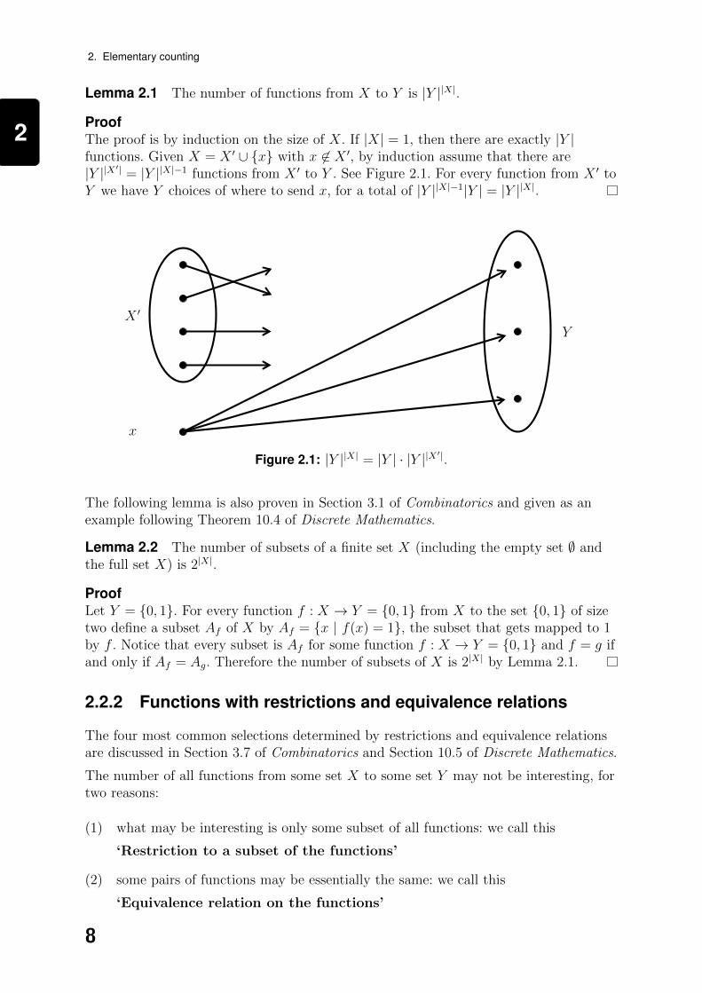
Lemma 2.1 The number of functions from X to Y is |Y ||X|.

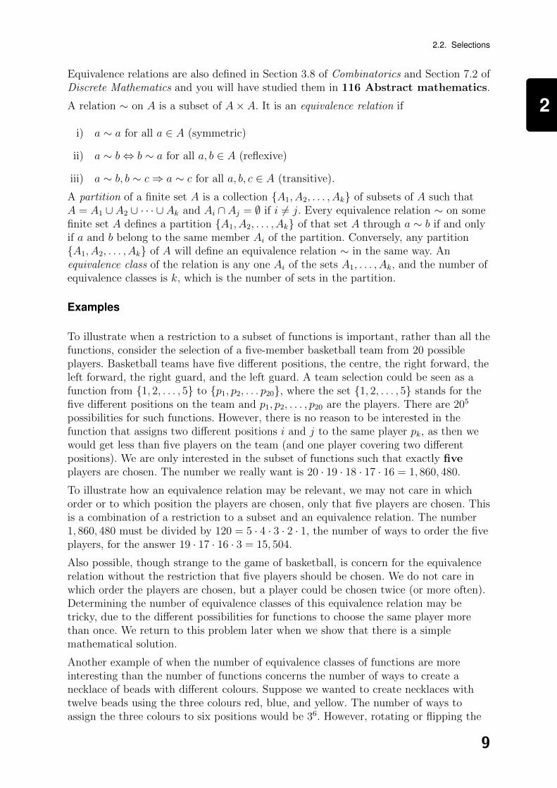
ProofThe proof is by induction on the size of X. If |X| = 1, then there are exactly |Y |functions. Given X = X ′ ∪ {x} with x 6∈ X ′, by induction assume that there are|Y ||X′| = |Y ||X|−1 functions from X ′ to Y . See Figure 2.1. For every function from X ′ toY we have Y choices of where to send x, for a total of |Y ||X|−1|Y | = |Y ||X|.

X ′

x

Y

Figure 2.1: |Y ||X| = |Y | · |Y ||X′|.

The following lemma is also proven in Section 3.1 of Combinatorics and given as anexample following Theorem 10.4 of Discrete Mathematics.

Lemma 2.2 The number of subsets of a finite set X (including the empty set ∅ andthe full set X) is 2|X|.

ProofLet Y = {0, 1}. For every function f : X → Y = {0, 1} from X to the set {0, 1} of sizetwo define a subset Af of X by Af = {x | f(x) = 1}, the subset that gets mapped to 1by f . Notice that every subset is Af for some function f : X → Y = {0, 1} and f = g ifand only if Af = Ag. Therefore the number of subsets of X is 2|X| by Lemma 2.1.

2.2.2 Functions with restrictions and equivalence relations

The four most common selections determined by restrictions and equivalence relationsare discussed in Section 3.7 of Combinatorics and Section 10.5 of Discrete Mathematics.

The number of all functions from some set X to some set Y may not be interesting, fortwo reasons:

(1) what may be interesting is only some subset of all functions: we call this

‘Restriction to a subset of the functions’

(2) some pairs of functions may be essentially the same: we call this

‘Equivalence relation on the functions’

8

2

2.2. Selections

Equivalence relations are also defined in Section 3.8 of Combinatorics and Section 7.2 ofDiscrete Mathematics and you will have studied them in 116 Abstract mathematics.

A relation ∼ on A is a subset of A× A. It is an equivalence relation if

i) a ∼ a for all a ∈ A (symmetric)

ii) a ∼ b⇔ b ∼ a for all a, b ∈ A (reflexive)

iii) a ∼ b, b ∼ c⇒ a ∼ c for all a, b, c ∈ A (transitive).

A partition of a finite set A is a collection {A1, A2, . . . , Ak} of subsets of A such thatA = A1 ∪ A2 ∪ · · · ∪ Ak and Ai ∩ Aj = ∅ if i 6= j. Every equivalence relation ∼ on somefinite set A defines a partition {A1, A2, . . . , Ak} of that set A through a ∼ b if and onlyif a and b belong to the same member Ai of the partition. Conversely, any partition{A1, A2, . . . , Ak} of A will define an equivalence relation ∼ in the same way. Anequivalence class of the relation is any one Ai of the sets A1, . . . , Ak, and the number ofequivalence classes is k, which is the number of sets in the partition.

Examples

To illustrate when a restriction to a subset of functions is important, rather than all thefunctions, consider the selection of a five-member basketball team from 20 possibleplayers. Basketball teams have five different positions, the centre, the right forward, theleft forward, the right guard, and the left guard. A team selection could be seen as afunction from {1, 2, . . . , 5} to {p1, p2, . . . p20}, where the set {1, 2, . . . , 5} stands for thefive different positions on the team and p1, p2, . . . , p20 are the players. There are 205

possibilities for such functions. However, there is no reason to be interested in thefunction that assigns two different positions i and j to the same player pk, as then wewould get less than five players on the team (and one player covering two differentpositions). We are only interested in the subset of functions such that exactly fiveplayers are chosen. The number we really want is 20 · 19 · 18 · 17 · 16 = 1, 860, 480.

To illustrate how an equivalence relation may be relevant, we may not care in whichorder or to which position the players are chosen, only that five players are chosen. Thisis a combination of a restriction to a subset and an equivalence relation. The number1, 860, 480 must be divided by 120 = 5 · 4 · 3 · 2 · 1, the number of ways to order the fiveplayers, for the answer 19 · 17 · 16 · 3 = 15, 504.

Also possible, though strange to the game of basketball, is concern for the equivalencerelation without the restriction that five players should be chosen. We do not care inwhich order the players are chosen, but a player could be chosen twice (or more often).Determining the number of equivalence classes of this equivalence relation may betricky, due to the different possibilities for functions to choose the same player morethan once. We return to this problem later when we show that there is a simplemathematical solution.

Another example of when the number of equivalence classes of functions are moreinteresting than the number of functions concerns the number of ways to create anecklace of beads with different colours. Suppose we wanted to create necklaces withtwelve beads using the three colours red, blue, and yellow. The number of ways toassign the three colours to six positions would be 36. However, rotating or flipping the

9

2


necklace results in the same necklace. For example, the necklace defined by the sequencey, y, b, r, b, r is the same necklace as that defined by the sequences r, b, r, b, y, y(flipping between beads) and is the same as that defined by the sequence y, r, b, r, b, y(rotating by one). All three of these functions define the same necklace. See Figure 2.2.Counting the number of necklaces is a problem of counting the number of equivalenceclasses, where two functions are equivalent if they define the same necklace. An effectivemethod for determining this number will be presented in a later chapter.

r b

r

by

y

Figure 2.2: Flip and rotate.

In general, given a subset A of all the functions and an equivalence relation defined by∼ we will want to know the number k such that there is a partition {A1, A2, . . . , Ak} ofA such that for all a, b ∈ A it holds that a ∼ b if and only if a, b ∈ Ai for some i.

The following definitions are given in Section 5.2 of Discrete Mathematics and in 116Abstract mathematics.

A function f : X → Y is injective if f(x) = f(y) implies that x = y.

The image of a function f : X → Y (im (f)) is the subset of all points in Y that aref(x) for some x in X.

A function f : X → Y is surjective if the image of f is the whole set Y .

A function that is both injective and surjective is called a bijection.

A bijective function from a set X to itself is called a permutation of X. See Figure 2.3.

Injective Surjective Bijective

Figure 2.3: Examples.

There are many types of subset restrictions and equivalence relations. But there are twopairs that are most commonly used. They are the same as those presented in Chapter

10

2

2.2. Selections

3.7 of Combinatorics and in Sections 10.5 and 11.2 of Discrete Mathematics. Weconsider the functions from a set X to a set Y .

1. Subsets of functions:

With repetitions: all functions from X to Y are relevant.

Without repetitions: only injective functions from X to Y are relevant.

2. Equivalence relations:

Ordered: no two distinct functions from X to Y are considered to be equivalent.

Unordered: permutations on X yield equivalent functions.

Permutations on Y yielding equivalent functions define a different equivalence relation.We deal with this later.

Four most common selections

Ordered with repetitions: this is the most inclusive. These are all the functions froma k-set to an n-set.

The best example is the number of different keys that can be made to open a lock. Atevery depth of the key there are finitely many positions. The width of the key has tomatch that of the lock for every position, otherwise the key will not work.

Ordered without repetitions: This is the subset of injective functions.

Suppose there is a cricket team of 20 players. The manager must choose not only 11players from the 20 on the team to bat, but also determine the batting order. For thefirst on the batting order, one of 20 can be chosen. For the second, one of 19 can bechosen, and so on. The number of such functions is 20 · 19 · · · 10.

The number n · (n− 1) · · · (n− k + 1) is called ‘n falling k’ and is denoted by (n)k. It isthe number of injective functions from a k-set to an n-set.

Obviously if k is larger than n then there can be no injective function, and then (n)k isdefined to be zero.

Unordered without repetitions: Only the injective functions are used, and allfunctions with the same image are equivalent.

For example, the above example of choosing 5 players from 20 to make a basketballteam is such a selection, where their positions or the order of their selection is notimportant nor considered.

The number (k)k = k · (k − 1) · · · 1 is denoted by k!. It is the number of bijective

functions from a k-set to itself. The number(n)kk!

is called ‘n choose k’, and is written

as

(n

k

)or as

n!

k!(n− k)!. This is also the number of k subsets of an n-set. If n is smaller

than k then (n)k and

(n

k

)would be 0 (as there would be no injective functions from a

k-set to an n-set) and

(n

0

)=

(n

n

)=

(0

0

)= 1. This is also presented in Section 3.2 of

Combinatorics.

11

2


Unordered with repetitions: There is a total of k objects and n different types orcolours. What matters is how many objects there are of each type or colour, but theobjects themselves have no identity.

Example 2.1 In a population of k = 7, there are people of the n = 4 blood types,A, B, C, and D. What are the possible distributions?

We can represent a distribution as a total of n− 1 dividers | between the k objectsthat are to be labelled (representing the division into n different classes). If there aretwo of type A, three of type B, none of type C, and two of type D, we can representthis as AA|BBB||DD.

There are n− 1 dividers and a distribution is determined by the location of thesedividers in a set of n+ k − 1 positions. Therefore the number of distributions is

(n+ k − 1

n− 1

)=

(n+ k − 1

k

).

This argument is made in Section 3.7 of Combinatorics and it is Theorem 11.2 ofDiscrete Mathematics.

Define n(k) to be n · (n+ 1) · (n+ 2) · · · (n+ k − 1). n(k) is called ‘n rising k’, and it is

the same as (n+ k − 1)k. We also have the simple identity

(n+ k − 1

n− 1

)=n(k)

k!.

In the above example we distributed people into blood types where the people had noidentities. We could also distribute coins or money to people where the coins or moneyhad no identity but the people do. This would be the same mathematical problem, butone must remember that the ‘people’ play different roles; in the former they are in thedomain of the function and have no identities while in the latter they are in the range ofthe function and do have identities. We deal in more detail with this problem in a laterchapter.

2.2.3 Pascal’s triangle

Now we look in more detail at

(n

k

)and its properties. This can also be found in

Section 11.1 of Discrete Mathematics and Section 3.3 of Combinatorics.

The following lemma is Theorem 11.1.1 of Discrete Mathematics.

Lemma 2.3 For n ≥ k > 0

(n

k

)=

(n− 1

k

)+

(n− 1

k − 1

).

ProofChoose any number i from 1 to n. The k subsets of {1, 2, . . . , n} can be made including

the number i or excluding the number i. By including we have

(n− 1

k − 1

)ways and by

excluding we have

(n− 1

k

)ways.

12

2

2.2. Selections

Lemma 2.3 gives one way to calculate

(n

k

)known as Pascal’s Triangle.

1

1 1

1 2 1

1 3 3 1

1 4 6 4 1

1 5 10 10 5 1

1 6 15 20 15 6 1

The following is proven in Section 3.3 of Combinatorics and Section 11.3 of DiscreteMathematics. It is known as the Binomial Theorem.

Lemma 2.4 (a+ b)n =n∑

k=0

(n

k

)akbn−k.

Proof (1)When n = 0 then

(0

0

)= 1 and we get 1 on both sides of the equation. By induction,

we can assume that

(a+ b)n−1 =n−1∑

k=0

(n− 1

k

)akbn−k−1.

It follows that

(a+ b)(a+ b)n−1 =n−1∑

k=0

(n− 1

k

)akbn−k +

n−1∑

k=0

(n− 1

k

)ak+1bn−k−1.

The latter sum can be re-written as

n∑

k=1

(n− 1

k − 1

)akbn−k.

Collecting together the terms for k ≥ 1 one gets the coefficient

(n− 1

k − 1

)+

(n− 1

k

)=

(n

k

)

(from Lemma 2.3). And for k = 0 one simply gets the coefficient

(n− 1

0

)which is 1

and equal to

(n

0

).

Proof (2)The number of unordered ways and without repetition to select k times the letter a and

n− k times the letter b is

(n

k

). This is exactly the coefficient for akbn−k in the

expression (a+ b)(a+ b) · · · (a+ b) repeated n times, which counts the number of kchoices for a with n− k choices for b.

13

2


Proof (3)Let D be the differential operator on the polynomials, meaning that Df of the

polynomial f(x) is the functiondf

dx. From elementary calculus there is Taylor’s formula,

which states that for all polynomials f

f(x+ y) = f(x) + [Df ](x)y + · · · [Dkf ](x)yk

k!+ · · · .

Letting f(t) be tn, it follows by substitution, as [Dkf ](x) = (n)kxn−k and

(n

k

)=

(n)kk!

.

Exercises for section 2.2

Exercise 2.1

How many results are possible when throwing 6 identical 6-sided dice?

Exercise 2.2

How many ways are there to roll two identical dice for a sum that is divisible by three?Likewise for a sum divisible by two?

Exercise 2.3

Assume that there are nine billiard balls, five of them are black and the other four arecoloured blue, yellow, red, and green. In how many ways can one choose five balls out ofthese nine (so that with respect to the black balls only their number is relevant)?

Exercise 2.4

Prove the formula for any integers n and k:

nk =k∑

j=0

(k

j

)(n− 1)j.

We proved using induction on the number k that nk is the number of functions from ak-set to an n-set. How can this formula be used to prove the same result usinginduction on the number n?

Exercise 2.5

Prove the formula for n ≥ 1 and s ≥ 1:

(s+ n

n

)=

(s− 1

0

)+

(s

1

)+

(s+ 1

2

)+ · · ·+

(s+ n− 1

n

).

2.3 Inclusion-exclusion

If in a room there are 17 adult men and 22 adult women then there are 39 adults. Why?

14

2

2.3. Inclusion-exclusion

First, all adults are either men or women, and second, nobody is both a man and awoman.

The North London football teams Arsenal and Tottenham are playing and people arewatching the game on TV in a pub. If 13 fans of Arsenal are watching and 8 fans ofTottenham are watching, how many people are watching? See Figure 2.4.

TV

Tottenham

fans

Arsenal fans

The Old White Lion

Figure 2.4: How many people are watching?

The equation 13 + 8 = 21 might be the wrong answer. First, there may be some peoplewatching who are not fans of either team. Second, some people may be fans of bothteams. If everyone is indeed a fan of one of the two teams and two of them are fans ofboth teams, then we know that 19 people are watching. We can calculate this in twoways. We can break things down into three categories: exclusive fans of Arsenal,exclusive fans of Tottenham, and fans of both, with 13− 2 = 11 of the first, 8− 2 = 6 ofthe second, and 2 of the third, and then add up for 11 + 6 + 2 = 19. Another way is toadd the 13 and 8 together, and then subtract the 2, the people who were counted twice.The second way is of greater mathematical sophistication.

2.3.1 The theorem

Proofs of the following theorem are in Sections 11.4 and 11.5 of Discrete Mathematicsand Section 5.1 of Combinatorics.

Theorem 2.5 (Inclusion-Exclusion) Let A1, A2, . . . , An be finite sets.∣∣∣∣∣n⋃

i=1

Ai

∣∣∣∣∣ =∑

∅6=K⊆{1,2,...,n}(−1)|K|+1

∣∣∣∣∣⋂

i∈KAi

∣∣∣∣∣ .

15

2


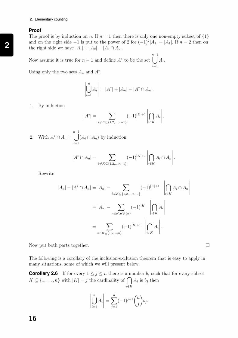
ProofThe proof is by induction on n. If n = 1 then there is only one non-empty subset of {1}and on the right side −1 is put to the power of 2 for (−1)2|A1| = |A1|. If n = 2 then onthe right side we have |A1|+ |A2| − |A1 ∩ A2|.

Now assume it is true for n− 1 and define A∗ to be the setn−1⋃

i=1

Ai.

Using only the two sets An and A∗,

∣∣∣∣∣n⋃

i=1

Ai

∣∣∣∣∣ = |A∗|+ |An| − |A∗ ∩ An|.

1. By induction

|A∗| =∑

∅6=K⊆{1,2,...,n−1}(−1)|K|+1

∣∣∣∣∣⋂

i∈KAi

∣∣∣∣∣ .

2. With A∗ ∩ An =n−1⋃

i=1

(Ai ∩ An) by induction

|A∗ ∩ An| =∑

∅6=K⊆{1,2,...,n−1}(−1)|K|+1

∣∣∣∣∣⋂

i∈KAi ∩ An

∣∣∣∣∣ .

Rewrite

|An| − |A∗ ∩ An| = |An| −∑

∅6=K⊆{1,2,...,n−1}(−1)|K|+1

∣∣∣∣∣⋂

i∈KAi ∩ An

∣∣∣∣∣

= |An| −∑

n∈K,K 6={n}(−1)|K|

∣∣∣∣∣⋂

i∈KAi

∣∣∣∣∣

=∑

n∈K⊆{1,2,...,n}(−1)|K|+1

∣∣∣∣∣⋂

i∈KAi

∣∣∣∣∣ .

Now put both parts together.

The following is a corollary of the inclusion-exclusion theorem that is easy to apply inmany situations, some of which we will present below.

Corollary 2.6 If for every 1 ≤ j ≤ n there is a number bj such that for every subset

K ⊆ {1, . . . , n} with |K| = j the cardinality of⋂

i∈KAi is bj then

∣∣∣∣∣n⋃

i=1

Ai

∣∣∣∣∣ =n∑

j=1

(−1)j+1

(n

j

)bj.

16

2


2.3.2 Applications

Application to co-primes

For any positive integer n the number φ(n) is defined to be the number of positiveintegers k less than n such that the greatest common divisor of k and n is 1, meaningthat the only positive integer that divides both k and n is the number 1. The followingapplication is presented in Section 11.5 of Discrete Mathematics.

Assume that n breaks down to n = pα11 p

α22 · · · pαq

q , where p1, p2, . . . , pq are distinct primeintegers.

To apply inclusion-exclusion, we need to determine first for every subset of primenumbers that divides the number n how many numbers less than or equal to n aredivided by this subset. Let A be any subset of {1, 2, . . . , q}. It is easy to calculate thatthe number of positive integers less than n divisible by all the primes in A is

n∏i∈A pi

,

the same as the number of positive integers less than or equal to n divided by∏

i∈Api.

Apply the inclusion-exclusion theorem to get

φ(n) = n−∑

A⊆{1,2,...,q}(−1)|A|+1 n∏

i∈A pi

= n

(1− 1

p1

)(1− 1

p2

)· · ·(

1− 1

pq

).

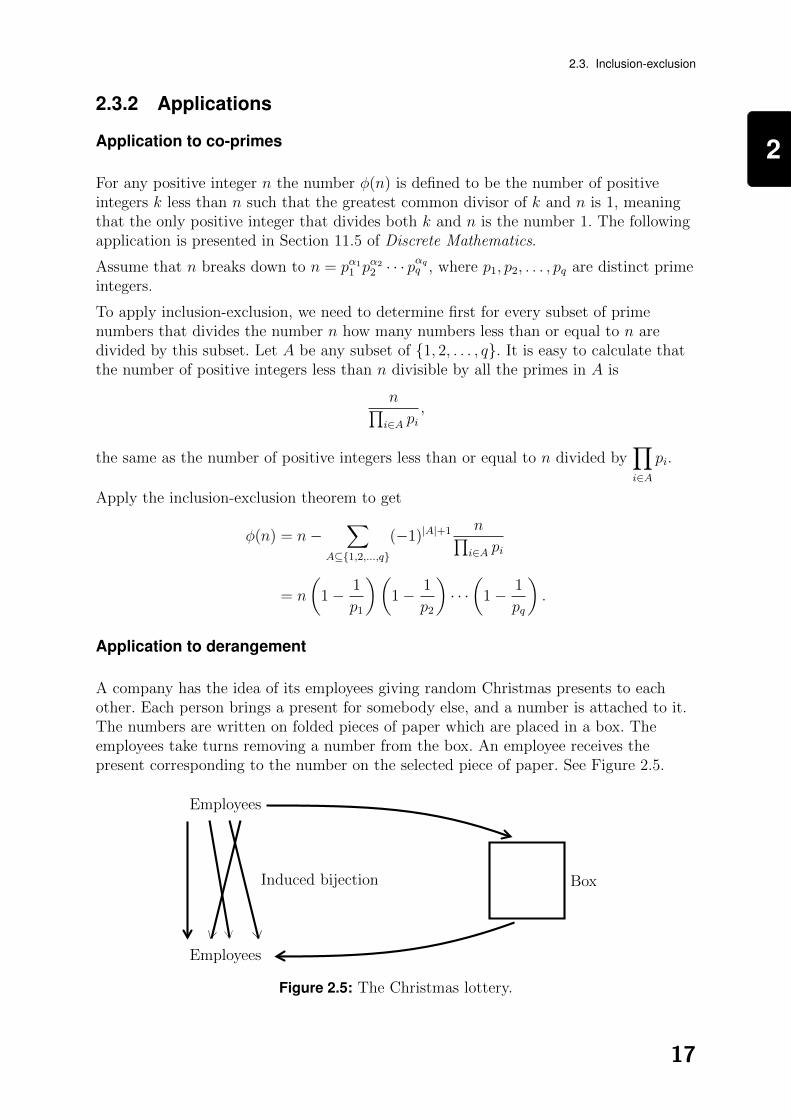
Application to derangement

A company has the idea of its employees giving random Christmas presents to eachother. Each person brings a present for somebody else, and a number is attached to it.The numbers are written on folded pieces of paper which are placed in a box. Theemployees take turns removing a number from the box. An employee receives thepresent corresponding to the number on the selected piece of paper. See Figure 2.5.

Employees

Induced bijection

Employees

Box

Figure 2.5: The Christmas lottery.

17

2


The only problem with this idea is the possibility that somebody gives their present tothemselves. If there are only two employees, this probability is one-half. If there arethree employees then this probability is 2

3(4 out of the six permutations).

What is the probability of somebody getting their own present if n is large? Will thisprobability converge, and if so to 0, 1, or something in between as n goes to infinity?This problem is treated in Section 11.4 of Discrete Mathematics.

Let N be the set of employees, and n = |N | its size. For every A ⊆ N the number ofpermutations of N such that all in A get their own presents is exactly the number ofpermutations of N\A, namely (n− |A|)!. For every k the number of subsets of N of size

k is

(n

k

).

By the inclusion-exclusion formula the number of permutations of N such that at leastone element is mapped to itself is

n∑

k=1

(−1)k+1

(n

k

)(n− k)! = n!

n∑

k=1

(−1)k+1

k!.

After dividing by n!, the total number of permutations, the probability that nobodygets their own present is

1−n∑

k=1

(−1)k+1

k!=

n∑

k=0

(−1)k

k!.

This is also presented in Theorem 5.1.3 of Combinatorics.

The Taylor formula for ex is∞∑

k=0

xk

k!. It follows that lim

n→∞

n∑

k=0

(−1)k

k!is e−1. Therefore the

probability that nobody gets their own present is e−1 in the limit, or about 0.368. If thecompany is big then the probability that somebody gets their own present is over 60 percent. Interestingly this probability is not monotone in the variable n. Even numbers ofelements give a slightly greater tendency for avoiding the situation where somebodygives a present to themselves.

2.3.3 Surjective functions

How many surjective functions are there from a k-set to an n-set? We can use theinclusion-exclusion method to get an answer.

We calculate the number of surjective functions from a k-set to an n-set by calculatingfirst the number of non-surjective functions. A function that is not surjective avoidssome subset of the n-set. The number of functions that avoids a subset of size j is(n− j)k, the total number of functions from a k-set to the other elements excluding thechosen set of size j. By inclusion-exclusion the number of non-surjective functions is

n∑

j=1

(−1)j+1

(n

j

)(n− j)k.

Therefore, the number of surjective functions is

nk −n∑

j=1

(−1)j+1

(n

j

)(n− j)k =

n∑

j=0

(−1)j(n

j

)(n− j)k.

18

2


This is presented in Theorem 5.1.2 in Combinatorics.

Surjective selections

3

2

1

2

1

τσ

f

3

2

1

2

1

f ◦ σ

3

2

1

2

1

τ ◦ f

Figure 2.6: How permutations change functions.

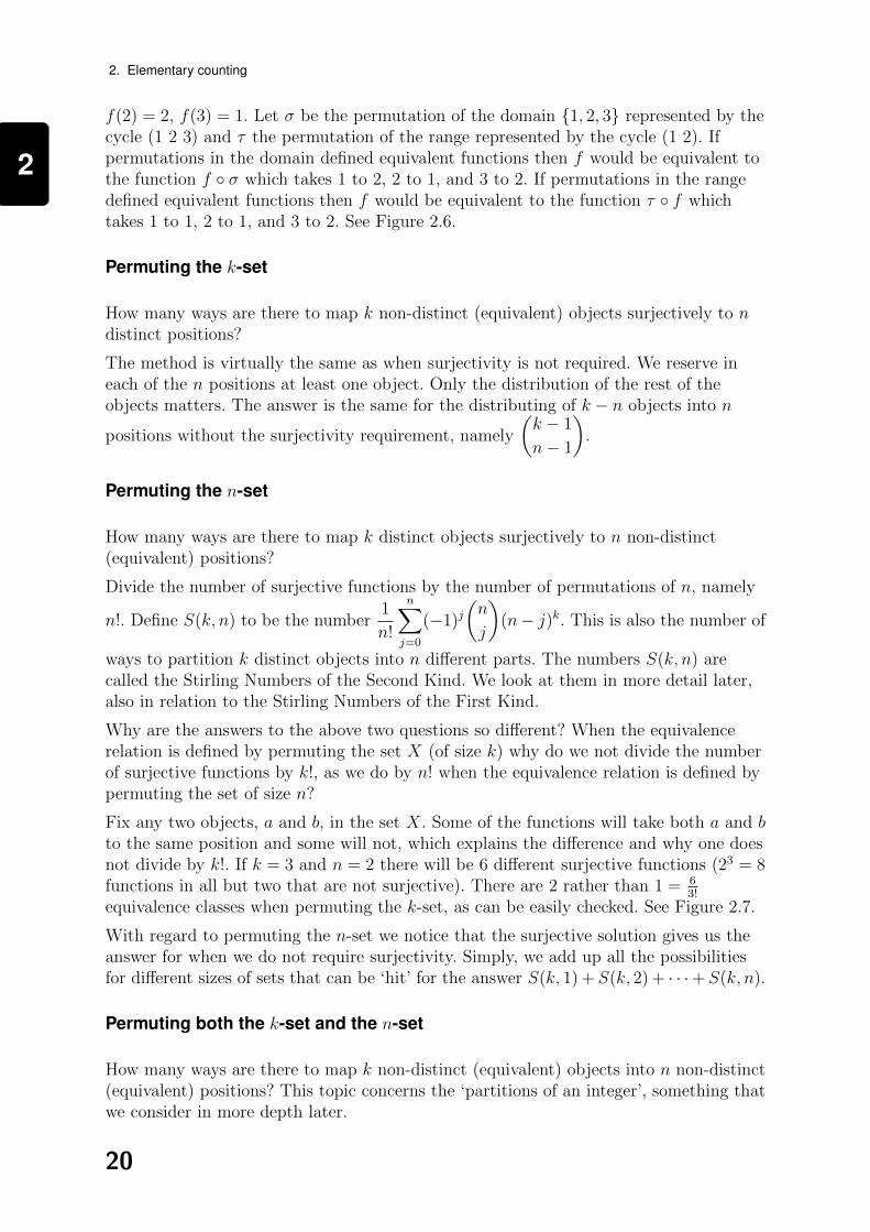
With regard to surjective functions from a k-set to an n-set there are at least two waysto define equivalence relations. One can permute the domain, the k-set. This is what wehave done so far. Also one can permute the range, the n-set. We count the number ofsurjective selections using both approaches. We discover that the solutions are not thatdifferent from the solutions when one does not require surjectivity.

What do we mean by the equivalence relationships defined by permuting the domainand permuting the range? Take the function f : {1, 2, 3} → {1, 2} defined by f(1) = 2,

19

2


f(2) = 2, f(3) = 1. Let σ be the permutation of the domain {1, 2, 3} represented by thecycle (1 2 3) and τ the permutation of the range represented by the cycle (1 2). Ifpermutations in the domain defined equivalent functions then f would be equivalent tothe function f ◦ σ which takes 1 to 2, 2 to 1, and 3 to 2. If permutations in the rangedefined equivalent functions then f would be equivalent to the function τ ◦ f whichtakes 1 to 1, 2 to 1, and 3 to 2. See Figure 2.6.

Permuting the k-set

How many ways are there to map k non-distinct (equivalent) objects surjectively to ndistinct positions?

The method is virtually the same as when surjectivity is not required. We reserve ineach of the n positions at least one object. Only the distribution of the rest of theobjects matters. The answer is the same for the distributing of k − n objects into n

positions without the surjectivity requirement, namely

(k − 1

n− 1

).

Permuting the n-set

How many ways are there to map k distinct objects surjectively to n non-distinct(equivalent) positions?

Divide the number of surjective functions by the number of permutations of n, namely

n!. Define S(k, n) to be the number1

n!

n∑

j=0

(−1)j(n

j

)(n− j)k. This is also the number of

ways to partition k distinct objects into n different parts. The numbers S(k, n) arecalled the Stirling Numbers of the Second Kind. We look at them in more detail later,also in relation to the Stirling Numbers of the First Kind.

Why are the answers to the above two questions so different? When the equivalencerelation is defined by permuting the set X (of size k) why do we not divide the numberof surjective functions by k!, as we do by n! when the equivalence relation is defined bypermuting the set of size n?

Fix any two objects, a and b, in the set X. Some of the functions will take both a and bto the same position and some will not, which explains the difference and why one doesnot divide by k!. If k = 3 and n = 2 there will be 6 different surjective functions (23 = 8functions in all but two that are not surjective). There are 2 rather than 1 = 6

3!

equivalence classes when permuting the k-set, as can be easily checked. See Figure 2.7.

With regard to permuting the n-set we notice that the surjective solution gives us theanswer for when we do not require surjectivity. Simply, we add up all the possibilitiesfor different sizes of sets that can be ‘hit’ for the answer S(k, 1) + S(k, 2) + · · ·+ S(k, n).

Permuting both the k-set and the n-set

How many ways are there to map k non-distinct (equivalent) objects into n non-distinct(equivalent) positions? This topic concerns the ‘partitions of an integer’, something thatwe consider in more depth later.

20

2


3

2

1

3

2

1

3

2

1

(a)

2

1

2

1

(b)

Figure 2.7: Surjective selections: (a) permuting the range, (b) permuting the domain.

Example 2.2 (Cards)When playing with a standard deck of 52 cards, in how many ways can a card playerreceive a hand of five cards with at least one card from each suit?

The total number of hands is

(52

5

). We count the number of possibilities of

receiving only cards from 3 or fewer suits, and subtract the result from

(52

5

).

Assuming the suits are numbered 1 through 4, for every proper subsetA ⊆ {1, 2, 3, 4} let HA be the set of hands that uses only the suits in A and let nA bethe number of hands which are made from only suits in the set A. This number nA is(

13|A|5

), and is determined only by the size of A. We need to calculate the size of

⋃

A⊆{1,2,3,4}HA. By inclusion-exclusion this number is

4

(39

5

)− 6

(26

5

)+ 4

(13

5

)−(

0

5

).

Subtracting from

(52

5

)gives the answer

(52

5

)− 4

(39

5

)+ 6

(26

5

)− 4

(13

5

)= 685, 464.

With the total number of hands being

(52

5

)= 2, 598, 960, we see that only about 26

per cent of all hands have all four suits.

There is another way to count this number. One of the suits must be represented bytwo cards, the rest by one. We choose one of four suits to be represented twice, and

then two representatives can be chosen in

(13

2

)= 78 ways. For each of the other

three suits we have a choice of one of 13 representatives. The answer is4 · 78 · 133 = 685, 464. It is valuable to look at both of these methods.

21

2



Exercise 2.6

How many integers from 1 to 106 (inclusive) are either squares or cubes?

Exercise 2.7

What is the number of surjective functions from a 6-set to a 4-set?

What is the number if the selection is unordered, meaning that only the number ofelements reaching each member of the 4-set is relevant?

Exercise 2.8

Define two functions from a 6-set to a 4-set to be equivalent if a permutation of the4-set transforms one function into the other function. There are 46 such functions, buthow many equivalence classes?

Exercise 2.9

Consider the functions from a k-set to an n-set and let two functions f, g be equivalentif f = g ◦ π where π is any permutation of the k-set. Find numbers k and n such thatmore than two-thirds of the functions are surjective however less than one-third of theequivalent classes contain surjective functions.

Exercise 2.10

In a standard deck of 52 cards, there are four suits and each suit has the numbers 1 to13 (with King=13 and Ace=1). A 4-hand is a set of 4 different cards from this deck.

(a) How many different 4-hands can a player receive?

(b) How many different 4-hands can a player receive such that all 4 cards are of thesame suit?

(c) How many different 4-hands can a player receive where there are exactly twonumbers present with two cards of each number?

A game is played with four players, each receiving a 4-hand. Player One holds in hishand all four cards of the number eight. The last three parts concern this situation ofPlayer One’s unusual 4-hand. Two ways are different if and only if some player holds adifferent hand.

(d) In how many different ways can the rest of the cards be distributed to the otherthree players?

(e) Of those ways from question (d), for how many will all three other players receivehands that contain four cards of the same suit?

(f) Of those ways from question (d) how many involve at least one of the other threeplayers also having four cards of the same number? Hint: use inclusion-exclusion.

22

2

2.4. Partitions and permutations

Exercise 2.11

How many ways are there to distribute 6 black balls (indistinguishable objects) and 6coloured balls (distinguishable objects with 6 distinct colours) to five distinguishablepeople so that three people get 2 objects and two people get 3 objects?

2.4 Partitions and permutations

Relevant to this section are Sections 3.5, 13.1 and 13.2 of Combinatorics and Sections12.1 to 12.5 of Discrete Mathematics.

2.4.1 Partitions of an integer

A partition of a positive integer k is a way to write k as a sum of positive integers. Forexample, the partitions of 5 are the following:

5

4 + 1 3 + 2

3 + 1 + 1 2 + 2 + 1

2 + 1 + 1 + 1

1 + 1 + 1 + 1 + 1

The above listing of the partitions of 5 are grouped according to the size of thepartition. 3 + 1 + 1 and 2 + 2 + 1 are the partitions of 5 into three parts. For everypositive integer n there will be only one partition into one part, namely n itself, andonly one partition into n parts, namely 1 + 1 + · · ·+ 1.

The partitions of an integer k are the equivalence classes of the functions from a k-setto a k-set when permutations of both the domain and the range of the function result inequivalent functions.

2.4.2 Partition and cycle types

The conventional notation for a partition of an integer k uses the form

[rm11 · rm2

2 · · · rmll ]

where k =l∑

i=1

rimi and r1 > r2 > · · · > rl and dropping the exponent means that it

should be 1. This is presented in Section 13.1 of Combinatorics and Section 12.4 ofDiscrete Mathematics.

The partition 3 + 1 + 1 of 5 is written as [3 · 12].

The partition 5 + 3 + 3 + 2 + 2 + 2 + 1 + 1 + 1 of 20 is written as [5 · 32 · 23 · 13].

A partition [rm11 · rm2

2 · · · rmll ] of an integer k is also called a type. To every such type and

every set A of size k there belong partitions and permutations of the set A. We presentthe relationship to partitions first.

23

2


2.4.3 Number of partitions

Every partition of a set A of cardinality k must come in the form

{A1r1, A2

r1, . . . , Am1

r1, . . . A1

r2, A2

r2, . . . , Am2

r2. . . A1

rl, A2

rl, . . . , Aml

rl

}

where for any pair i, j the cardinality of Aij is rj, k =l∑

i=1

rimi and r1 > r2 > · · · > rl.

This structure uniquely defines a type, namely[rm11 · rm2

2 · · · rmll

]. For example, the

partition {{1, 3, 4}, {2, 5, 9}, {6, 7}, {8}, {10}} belongs to the type[32 · 2 · 12

].

The following lemma can be deduced from Proposition 13.1.5 of Combinatorics.

Lemma 2.7 The number of partitions of a set of cardinality k belonging to the type[rm1

1 · rm22 · · · rml

l ] isk!

(r1!)m1 · · · (rl!)mlm1! · · ·ml!.

ProofWe proceed by induction on l. Assume that l = 1 (and therefore k = r1m1). Let us

choose the partition members. For the first partition member we have a choice of

(k

r1

)

objects. For the second partition member we have a choice of

(k − r1r1

)objects. The

total number of possibilities is

(k

r1

)·(k − r1r1

)· · ·(r1r1

)=

k! · (k − r1)! · · · r1!(k − r1)! · (k − 2r1)! · · · 0! · (r1!)m1

=k!

(r1!)m1.

But any permutation on the m1 sets of size r1 yields the same partition, and thereforethe number of partitions is

k!

(r1!)m1m1!.

Now assume that the lemma holds for the quantity l − 1. Every partition of kcorresponding to the type [rm1

1 · rm22 · · · rml

l ] defines a partition of a set of size r1m1

according to the type [rm11 ] and a partition of a set of size k − r1m1 belonging to the

type [rm22 · · · rml

l ]. Vice-versa, due to r1 6= ri for all i > 1, distinct choices for a set of sizer1m1 (determining a complementary choice of a set of size k − r1m1) followed bydistinct choices for the partitions of the r1m1-set and partitions of the (k − r1m1)-setcorresponding to the types [r1m1] and [rm2

2 · · · rmll ] respectively generate distinct

partitions of the k-set. Therefore the number of partitions of the k-set is

(k

r1m1

)r1m1!

(r1!)m1m1!

k − r1m1!

(r2!)m2 · · · (rl!)mlm2! · · ·ml!=

k!

(r1!)m1 · · · (rl!)mlm1! · · ·ml!.

24

2


We have a formula for the number of surjective functions from a k-set to an n-set andtherefore also a formula for the number of partitions of a k-set into n parts. For everytype of a k-set partitioned into n parts we know from Lemma 2.7 the number ofpartitions belonging to it. These numbers should match up.

Example 2.3 Consider the surjective functions from a 5-set to a 3-set.

By the formula the number of surjective functions is

35 −(

3

1

)(3− 1)5 +

(3

2

)(3− 2)5 = 243− 96 + 3 = 150.

The number of partitions of a 5-set into 3 parts is therefore150

3!=

150

6= 25.

Now consider the same task using the formula from Lemma 2.7 . A 5-set can bepartitioned into three parts in two ways, as the type [3 · 12] or as the type [22 · 1]. For

the first our formula gives5!

3! · 2!= 10 partitions and for the second our formula

gives5!

(2!)2 · 2!= 15 partitions.

The same classification scheme can be applied to the set of all functions of a k-set to ann-set.

We can break down these functions:

1. according to the sizes m = 1, 2, . . . , n of the image

2. then according to a set for that image

3. then according to the types, and finally

4. to the corresponding partitions for each type.

Example 2.4 Consider the set of all functions from a 5-set to a 3-set.

We have already considered the types with 3 parts. Next, consider the types with 2parts. These are [4 · 1] and [3 · 2]. According to Lemma 2.7:

the number of partitions corresponding to type [4 · 1] should be5!

4! · 1!= 5, and

the number of partitions corresponding to type [3 · 2] should be5!

3! · 2!= 10.

The total number of partitions should be 15, meaning that the correspondingnumber of functions should be 30 (multiplying by 2!). According to the formula thenumber of surjective functions from a 5-set to a 2-set should be 25 − 2 = 30.

Now consider the only type [5] of length 1. The number of partitions correspondingto this type is one. The number of surjective functions (from a 5-set to a 1-set) islikewise 1.

25

2


Now add up all the results. The number of functions from a 5-set to a 3-set should be

(3

3

)150 +

(3

2

)30 +

(3

1

)1 = 150 + 90 + 3 = 243 = 35.

2.4.4 Permutations

Permutations are bijective functions from a finite set to itself. There are k!permutations of a k-set.

We could express a permutation π as a function, with π(i) = ai and then list the resultsin the proper order:

1→ a1, 2→ a2, · · · , k → ak.

But there is a much more efficient way of expressing a permutation. Look at where thefirst element 1 goes, namely π(1). Then look at where this goes, (π ◦ π)(1) = π2(1). Wecould continue until some number i = πj(1) = πj+l(1) is repeated for the first time, andfrom then on cyclic repetition would rule:

1, π(1), π2(1), . . . , πj(1) = i, πj+1(1) = π(i), . . . , πj+l(1) = i.

But because the permutation π is a bijection, we could move backwards with its inverseπ−1 and show that πj+l−1(1) = πj−1(1) and so on backwards to 1 = πl(1). So startingfrom any element we get a cycle of elements returning to this first element. This allowsus to write down any permutation of a k-set as a partition of the k-set plus a cyclicorientation of each partition. See Figure 2.8.

Figure 2.8: A permutation in S18 with type [6 · 42 · 2 · 12].

For example, with k = 9, the following expression for a permutation

(1 5 3) (2 9) (8) (7 4 6)

means that 1 is mapped to 5, 5 is mapped to 3, 3 is mapped to 1, and so on, with 8mapped to itself. This is presented in Section 3.5 of Combinatorics and Section 10.6 ofDiscrete Mathematics.

26

2


Because any permutation of the k-set is based on a partition of the k-set, thepermutations are also classified according to their types.

A permutation π2 is conjugate to π1 if there exists another permutation ρ such thatρ−1π1ρ = π2.

Conjugacy is an equivalence relation,

(i) reflexive: use the identity permutation itself

(ii) symmetric: π1 = ρ−1π2ρ⇔ π2 = ρπ1ρ−1

(iii) transitive: π1 = ρ−1π2ρ, π2 = θ−1π3θ implies that π1 = ρ−1θ−1π3θρ.

Conjugating a permutation π by the permutation ρ is a way to represent the samepermutation π but with the names of the elements changed according to ρ. Aconjugation is the same concept as a basis change in linear algebra. Therefore thefollowing lemma, also Proposition 13.1.4 of Combinatorics and Theorem 12.5 of DiscreteMathematics, should not be surprising.

Lemma 2.8 Any two permutations are conjugate if and only if they have the sametype.

ProofAssume that permutations π1 and π2 have the same type and we pair cycles from bothof the same size. Choose any pairing of cycles with size m, the first a cycle of π1 and thesecond a cycle of π2:

(i1, i2, · · · , im) (j1, j2, · · · , jm).

Define a function ρ from the members of the first cycle to those of the second byρ(im) = jm. See Figure 2.9. Extend this function by doing the same for all pairs ofcycles, to a permutation on the whole set. We see that ρ−1 ◦ π2 ◦ ρ (il) will beil+1 = π1(il) (or, if l = m, then i1).

On the other hand, assuming a conjugacy between π1 and π2 with ρ−1π2ρ = π1, wechoose any cycle (j1, j2, · · · , jm) of π2 and define i1 to be ρ−1(j1). By ρ−1π2ρ = π1 itfollows that

πm1 (i1) = (ρ−1π2ρ)m(i1) = ρ−1 ◦ πm2 ◦ ρ (i1) = ρ−1 ◦ πm2 (j1) = ρ−1 (j1) = i1

(because πm2 (j1) = j1). On the other hand, if πn1 (i1) = i1 for some n strictly smaller thanm, we would have

i1 = πn1 (i1) = (ρ−1π2ρ)n(i1) = ρ−1 ◦ πn2 ◦ ρ(i1) = ρ−1 ◦ πn2 (j1).

But ρ could be applied on the left side for j1 = ρ(i1) = πn2 (j1), a contradiction.Therefore ρ−1 maps the cycle (j1, · · · , jm) to a cycle (i1, · · · , im), both of size m.Repeating the argument for all the cycles shows that they have the same cycle type.

The following lemma is also Proposition 13.1.5 of Combinatorics and is presented inSection 12.5 of Discrete Mathematics.

27

2


π1

im

i1i2 i3

i4

π2

jm

j1j2 j3

j4

ρ

Figure 2.9: Matching cycles.

Lemma 2.9 The number of permutations of a k-set corresponding to a type[rm1

1 · rm22 · · · rml

l ] isk!

rm11 · · · rml

l m1! · · ·ml!.

ProofEvery permutation of {1, . . . , k} generates a partition of {1, . . . , k} defined by thecycles. For every partition member of size ri, by fixing any element to come first, thereare (ri − 1)! ways to define a cycle using the rest of the elements. See Figure 2.10.Therefore to go from the number of partitions to the number of cycles corresponding tothe type we must multiply by ((r1 − 1)!)m1 · · · ((rl − 1)!)ml .

Just as above, we can check this formula.

Example 2.5 Consider the permutations of a 5-set. We list the types and thecorresponding number of permutations.

[5]5!

5= 24

[4 · 1]5!

4= 30

[3 · 2]5!

3 · 2 = 20

[3 · 12]5!

3 · 2!= 20

28

2


[22 · 1]5!

22 · 2!= 15

[2 · 13]5!

2 · 3!= 10

[15]5!

5!= 1

The total number of permutations is then 24 + 30 + 20 + 20 + 15 + 10 + 1 = 120 = 5!.

ar

a1

a2

(a1 a2 a3 . . . ar−1 ar)

(a2 a3 a4 . . . ar a1)

...

(ar a1 a2 . . . ar−2 ar−1)

Figure 2.10: Equivalent cycles.

2.4.5 Ferrers diagrams

Ferrers diagrams are presented in Section 13.1 of Combinatorics and Sections 26.1 and26.2 of Discrete Mathematics. There is a convenient way to express a particular partitionof k (a type), called a Ferrers diagram. We express [1 · 22 · 4 · 6], a partition of 15.

◦ ◦ ◦ ◦ ◦ ◦◦ ◦ ◦ ◦◦ ◦◦ ◦◦

29

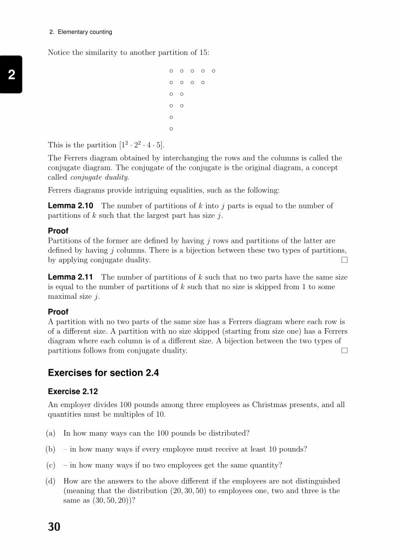
2


Notice the similarity to another partition of 15:

◦ ◦ ◦ ◦ ◦◦ ◦ ◦ ◦◦ ◦◦ ◦◦◦

This is the partition [12 · 22 · 4 · 5].

The Ferrers diagram obtained by interchanging the rows and the columns is called theconjugate diagram. The conjugate of the conjugate is the original diagram, a conceptcalled conjugate duality.

Ferrers diagrams provide intriguing equalities, such as the following:

Lemma 2.10 The number of partitions of k into j parts is equal to the number ofpartitions of k such that the largest part has size j.

ProofPartitions of the former are defined by having j rows and partitions of the latter aredefined by having j columns. There is a bijection between these two types of partitions,by applying conjugate duality.

Lemma 2.11 The number of partitions of k such that no two parts have the same sizeis equal to the number of partitions of k such that no size is skipped from 1 to somemaximal size j.

ProofA partition with no two parts of the same size has a Ferrers diagram where each row isof a different size. A partition with no size skipped (starting from size one) has a Ferrersdiagram where each column is of a different size. A bijection between the two types ofpartitions follows from conjugate duality.


Exercise 2.12

An employer divides 100 pounds among three employees as Christmas presents, and allquantities must be multiples of 10.

(a) In how many ways can the 100 pounds be distributed?

(b) – in how many ways if every employee must receive at least 10 pounds?

(c) – in how many ways if no two employees get the same quantity?

(d) How are the answers to the above different if the employees are not distinguished(meaning that the distribution (20, 30, 50) to employees one, two and three is thesame as (30, 50, 20))?

30

2

2.5. The Stirling numbers

Exercise 2.13

Show that the number of partition of an integer n into distinct and odd parts is equalto the number of partitions of the integer n that are self-conjugate (meaning that theFerrers diagram and its conjugate are the same).

Exercise 2.14

Let n and r be positive integers. Show that the number of partitions of n in which thenumber of parts is r or less is equal to the number of partitions of n+ r with exactly rparts.

2.5 The Stirling numbers

In the previous section we looked at the number of partitions and permutationsbelonging to the various types of a partition of an integer. One can aggregate this countaccording to the number of sets in the partition and the number of parts in thepermutation. The result is a surprising relationship between these numbers and certainpolynomials that are created in a very natural way.

The Stirling numbers are presented in Sections 5.3 and 15.6 of Combinatorics andSection 12.1 of Discrete Mathematics.

2.5.1 Stirling numbers of the first kind

(x)k = x(x− 1)(x− 2) · · · (x− k + 1),

x falling k, is a polynomial of degree k in the variable x and can be also written as

(x)k = s(k, k) xk + s(k, k − 1) xk−1 + · · ·+ s(k, 0),

with integers s(k, n).

The s(k, n) are called the Stirling numbers of the first kind.

Let us work out a few:

(x)0 = 1, (x)1 = x so

s(1, 1) = 1, s(1, 0) = 0.

(x)2 = x(x− 1) = x2 − x, so

s(2, 2) = 1, s(2, 1) = −1, s(2, 0) = 0.

(x)3 = (x− 2)(x2 − x) = x3 − 3x2 + 2x, so

s(3, 3) = 1, s(3, 2) = −3, s(3, 1) = 2, s(3, 0) = 0.

31

2


(x)4 = (x− 3)(x3 − 3x2 + 2x) = x4 − 6x3 + 11x2 − 6x, so

s(4, 4) = 1, s(4, 3) = −6, s(4, 2) = 11, s(4, 1) = −6, s(4, 0) = 0.

2.5.2 Stirling numbers of the second kind

S(k, n) is defined to be the number of partitions of a k-set into n parts, and thesenumbers are called the Stirling numbers of the second kind. We show how they relate tothe Stirling numbers of the first kind, something also presented in Section 5.3 ofCombinatorics..

Because (x)k, (x)k−1, . . . , (x)0 = 1 form a basis of the vector space of all polynomialswith real coefficients of degree k or less (just as the xk, xk−1, . . . , 1 do the same), wecan write

xk =k∑

j=0

R(k, j)(x)j

for some real numbers R(k, j). By substitution, xk =k∑

j=0

R(k, j)(x)j can be expanded to

xk =k∑

j=0

R(k, j)

j∑

m=0

s(j,m)xm.

With R(k, j) = s(k, j) = 0 if j > k the matrices defined by the R(k, j) and the s(k′, j′)are inverses of each other, meaning that

k∑

j=0

R(k, j)s(j,m) =

1, k = m,

0, k 6= m.

Lemma 2.12 The R(k, j) satisfy

R(0, 0) = 1, R(k, k) = 1, R(k, j) = R(k, 0) = 0

for all j > k ≥ 1, and

R(k, j) = jR(k − 1, j) +R(k − 1, j − 1)

for all 1 ≤ j ≤ k.

ProofR(0, 0) = 1, R(1, 1) = 1 and R(1, 0) = 0 come from 1 = (x)0 and x = (x)1.

Consider the equation xk = xxk−1. Substituting on both sides we have

k∑

j=0

R(k, j)(x)j =k−1∑

j=0

x R(k − 1, j)(x)j.

The x(x)j can be re-written as

(x)j(x− j) + j(x)j = (x)j+1 + j(x)j.

32

2


So the above equation can be re-written again as

k∑

j=0

R(k, j)(x)j =k−1∑

j=0

R(k − 1, j)(x)j+1 + j

k−1∑

j=0

R(k − 1, j)(x)j

=k∑

j=1

R(k − 1, j − 1)(x)j + j

k−1∑

j=0

R(k − 1, j)(x)j.

Since the (x)j form a basis of the polynomial vector space, if we fix any value for j thecoefficients should be equal.

Choosing j = k, we get R(k, k) = R(k − 1, k − 1), and by induction we have R(k, k) = 1for all k.

Choosing j = 0, we get R(k, 0) = jR(k − 1, 0), and again by induction we haveR(k, 0) = 0 for all k.

Choosing 0 < j < k we get R(k, j) = R(k − 1, j − 1) + j R(k − 1, j).

The following lemma is Theorem 12.1 of Discrete Mathematics.

Lemma 2.13 The Stirling numbers of the second kind, S(k, n), satisfy

S(0, 0) = 1, S(k, k) = 1, S(k, n) = S(k, 0) = 0

for all n > k ≥ 1, and

S(k, n) = nS(k − 1, n) + S(k − 1, n− 1)

for all 1 ≤ n ≤ k.

ProofA partition of {1, 2, . . . k} into n parts induces a partition of {1, 2, . . . , k − 1}, intoeither n or n− 1 parts. If k is alone in the partition, then we get a partition of k − 1objects into n− 1 parts. If k was not alone then we get a partition of k − 1 objects inton parts with n choices for where to put the last object k. See Figure 2.11.

k

1

2

n

Figure 2.11: k is not alone.

Corollary 2.14 The R(k, n) are the same as the S(k, n).

33

2


ProofThe two collections of numbers obey the same initial conditions and the samerecurrence relations.

2.5.3 Number of permutations

Now we show how the Stirling numbers of the first kind relate to the number ofpermutations. This is worked out in Section 5.3 of Combinatorics, in particular inProposition 5.3.3. Recall the definition of n rising k, n(k) = n · (n+ 1) · · · (n+ k − 1).

Lemma 2.15 The s(k, n) satisfy s(k, 0) = 0, s(k, k) = 1 and

s(k + 1, n) = s(k, n− 1)− ks(k, n)

for all k ≥ 1.

ProofThe first identities are trivial. For the last equation by definition (x)k+1 = (x)k(x− k)holds, yielding

s(k + 1, k + 1)xk+1 + · · ·+ s(k + 1, n)xn + · · ·+ s(k + 1, 0)

= (x− k)(s(k, k)xk + s(k, n)xn + s(k, n− 1)xn−1 + · · ·+ s(k, 0)

).

Looking at the nth power of this polynomial we get

s(k + 1, n) = s(k, n− 1)− ks(k, n).

Define the number c(k, n) to be the number of permutations of {1, 2, . . . , k} withexactly n cycles. Define c(0, 0) to be 1.

Lemma 2.16 The c(k, n) satisfy c(0, 0) = 1, c(k, 0) = 0 for all k ≥ 1, and

c(k, n) = (k − 1)c(k − 1, n) + c(k − 1, n− 1).

ProofFor k = 1 we have c(1, 1) = c(0, 0) = 1. For k ≥ 2 consider the permutation on{1, 2, . . . , k − 1} induced by removing from a permutation π on {1, 2, . . . , k} the lastelement k in the following way: if i goes to k and k goes to j then with the inducedpermutation i goes to j. Either the last element k is alone in a cycle of π, or it was in acycle of π with others.

If k is in a cycle alone, we generate a permutation ρ of {1, 2, . . . , k− 1} with n− 1 cycles.

If k is in a cycle with others we generate a permutation ρ of {1, 2, . . . , k − 1} with ncycles.

For any permutation ρ of {1, 2, . . . , k − 1} with n cycles we want to consider how manypermutations π of {1, 2, . . . , k} with n cycles will generate ρ. k could be inserted in anyof the cycles of ρ. For each cycle putting k back in the front of the cycle or at the back

34

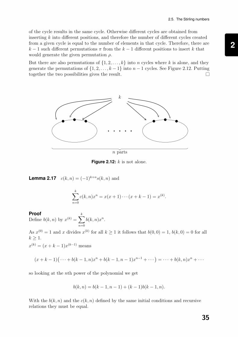
2


of the cycle results in the same cycle. Otherwise different cycles are obtained frominserting k into different positions, and therefore the number of different cycles createdfrom a given cycle is equal to the number of elements in that cycle. Therefore, there arek − 1 such different permutations π from the k − 1 different positions to insert k thatwould generate the given permutation ρ.

But there are also permutations of {1, 2, . . . , k} into n cycles where k is alone, and theygenerate the permutations of {1, 2, . . . , k− 1} into n− 1 cycles. See Figure 2.12. Puttingtogether the two possibilities gives the result.

k

n parts

Figure 2.12: k is not alone.

Lemma 2.17 c(k, n) = (−1)k+ns(k, n) and

k∑

n=0

c(k, n)xn = x(x+ 1) · · · (x+ k − 1) = x(k).

ProofDefine b(k, n) by x(k) =

k∑

n=0

b(k, n)xn.

As x(0) = 1 and x divides x(k) for all k ≥ 1 it follows that b(0, 0) = 1, b(k, 0) = 0 for allk ≥ 1.

x(k) = (x+ k − 1)x(k−1) means

(x+ k − 1)(· · ·+ b(k − 1, n)xn + b(k − 1, n− 1)xn−1 + · · ·

)= · · ·+ b(k, n)xn + · · ·

so looking at the nth power of the polynomial we get

b(k, n) = b(k − 1, n− 1) + (k − 1)b(k − 1, n).

With the b(k, n) and the c(k, n) defined by the same initial conditions and recursiverelations they must be equal.

35

2


Next replace x by −x for

k∑

n=0

c(k, n)(−x)n = −x(1− x) · · · (k − 1− x)

= (−1)kx(x− 1) · · · (x− k + 1)

= (−1)k(x)n

= (−1)kk∑

n=0

s(k, n)xn.

This implies that c(k, n) = (−1)k+ns(k, n).

Example 2.6 We calculate S(5, n) and s(5, n) for 0 ≤ n ≤ 5 using two methods:the previous method and then using (x)k.

Recall from Examples 2.3 and 2.4 we had

S(5, 1) = 1, S(5, 2) = 15, S(5, 3) = 25.

Furthermore S(5, 5) = 1 and using the formula

S(5, 4)4! = 45 − 4 · 35 + 6 · 25 − 4 · 15

= 1024− 972 + 192− 4

= 240

we get S(5, 4) = 10.

The number of permutations of a 5-set with n cycles was calculated to be:

n = 1 one type 24

n = 2 two types 50

n = 3 two types 35

n = 4 one type 10

n = 5 one type 1.

This means

s(5, 1) = 24, s(5, 2) = −50, s(5, 3) = 35, s(5, 4) = −10, s(5, 5) = 1.

Now find the Stirling number s(5, n) and S(5, n) using (x)k:

(x)4 = (x− 3)(x3 − 3x2 + 2x) = x4 − 6x3 + 11x2 − 6x

(x)5 = (x− 4)(x4 − 6x3 + 11x2 − 6x) = x5 − 10x4 + 35x3 − 50x2 + 24x.

36

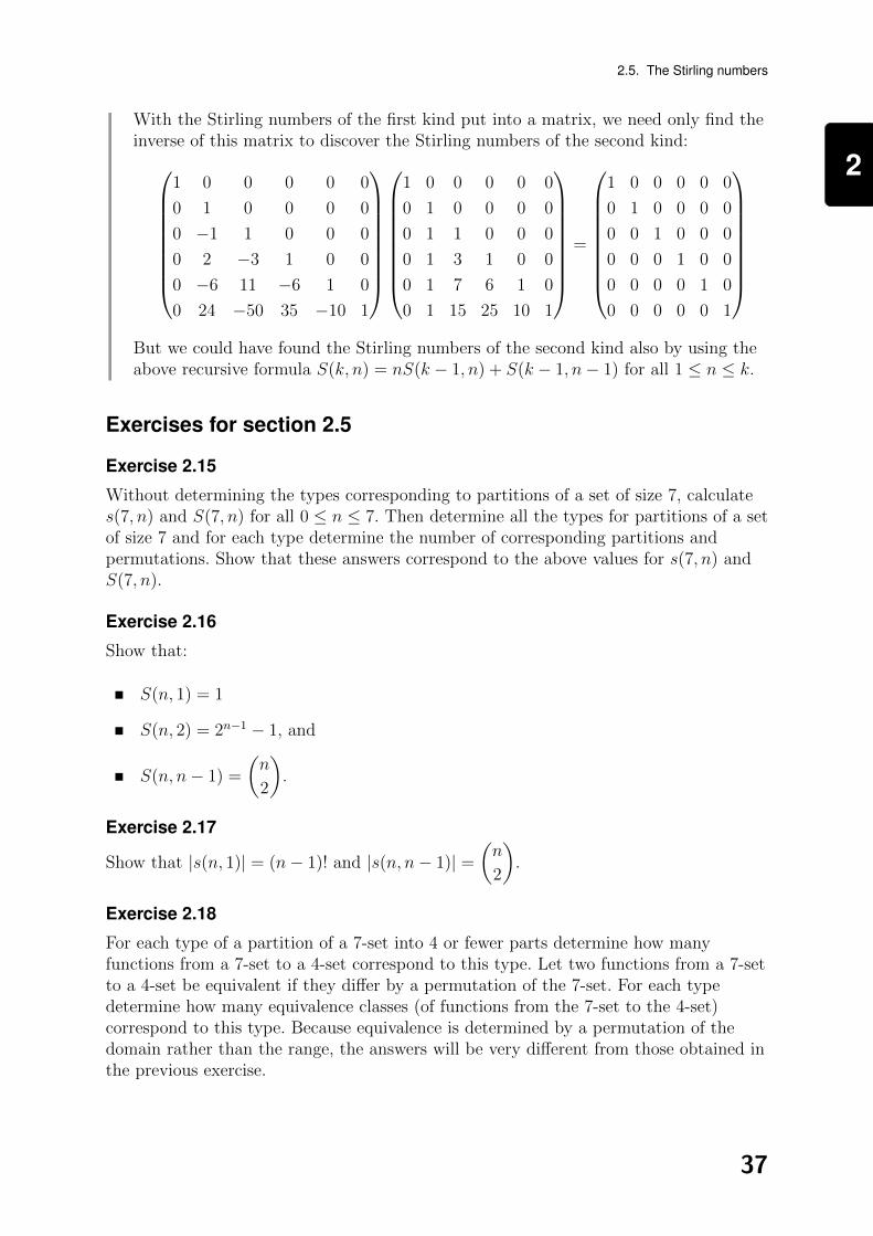
2


With the Stirling numbers of the first kind put into a matrix, we need only find theinverse of this matrix to discover the Stirling numbers of the second kind:

1 0 0 0 0 0

0 1 0 0 0 0

0 −1 1 0 0 0

0 2 −3 1 0 0

0 −6 11 −6 1 0

0 24 −50 35 −10 1

1 0 0 0 0 0

0 1 0 0 0 0

0 1 1 0 0 0

0 1 3 1 0 0

0 1 7 6 1 0

0 1 15 25 10 1

=

1 0 0 0 0 0

0 1 0 0 0 0

0 0 1 0 0 0

0 0 0 1 0 0

0 0 0 0 1 0

0 0 0 0 0 1

But we could have found the Stirling numbers of the second kind also by using theabove recursive formula S(k, n) = nS(k − 1, n) + S(k − 1, n− 1) for all 1 ≤ n ≤ k.


Exercise 2.15

Without determining the types corresponding to partitions of a set of size 7, calculates(7, n) and S(7, n) for all 0 ≤ n ≤ 7. Then determine all the types for partitions of a setof size 7 and for each type determine the number of corresponding partitions andpermutations. Show that these answers correspond to the above values for s(7, n) andS(7, n).

Exercise 2.16

Show that:

S(n, 1) = 1

S(n, 2) = 2n−1 − 1, and

S(n, n− 1) =

(n

2

).

Exercise 2.17

Show that |s(n, 1)| = (n− 1)! and |s(n, n− 1)| =(n

2

).

Exercise 2.18

For each type of a partition of a 7-set into 4 or fewer parts determine how manyfunctions from a 7-set to a 4-set correspond to this type. Let two functions from a 7-setto a 4-set be equivalent if they differ by a permutation of the 7-set. For each typedetermine how many equivalence classes (of functions from the 7-set to the 4-set)correspond to this type. Because equivalence is determined by a permutation of thedomain rather than the range, the answers will be very different from those obtained inthe previous exercise.

37

2


Learning outcomes

At the end of this chapter and the relevant reading, you should be able to:

count the functions from a k-set to an n-set according to various restrictions andequivalence relationsapply the inclusion-exclusion formula in various wayscount partitions and permutations according to their typesinterpret a Ferrers diagramcalculate explicitly the Stirling numbers of the first and second kinds for small kand n in various ways.

Solutions to exercises

Solutions to section 2.2 exercises

Solution to exercise 2.1

The throw of six identical dice yields six unordered choices of six different values. Sixobjects are divided by five dividers (for the six possible values), for a total of(

11

5

)= 462 results.


Concerning the rolling of two dice:

To roll a sum of 2, there is only 1 + 1.

To roll a sum of 4, there are 1 + 3 and 2 + 2.

To roll a sum of 6, there are 1 + 5, 2 + 4 and 3 + 3.


To roll a sum of 10, there are 4 + 6 and 5 + 5.


In total, there are 12 ways. But there are 21 ways to roll the dice, and yet theprobability of getting an even number is the same as getting an odd number. Thereason for this mismatch is simple: for each i ∈ {1, 2, 3, 4, 5, 6} the probability to rolli+ i is 1

36while the probability to roll i+ j for j 6= i is 1

18.



To roll a sum of 9, there are 3 + 6, and 4 + 5.

38

2

2.5. Solutions to exercises


In total, there are seven ways, exactly one third of the twenty-one.


Any choice of a non-empty subset of the coloured balls can be augmented by the rightnumber of black balls. So there are 24 ways to choose these balls, the number of subsetsof a 4-set.


Consider nk = ((n− 1) + 1)k and using the binomial expansion we get

nk =k∑

j=0

(k

j

)(n− 1)j1k−j =

k∑

j=0

(k

j

)(n− 1)j.

Now prove that nk is the number of functions from a k-set to an n-set using inductionon n rather than on k. If |n| = 1 then there is exactly one function and the formula istrue. Let x be any fixed element of the n-set and for every such function f let x(f) be

the number of elements of the k-set that reach x. With j fixed there are

(k

j

)(n− 1)j

different functions f such that x(f) = k − j, the (n− 1)j by the induction hypothesis

and the

(k

j

)being the number of choices for k − j elements to be mapped to x.

Therefore by induction hypothesis there arek∑

j=0

(k

j

)(n− 1)j different functions from a

k-set to an n-set, and we have shown that this is equal to nk.


Order the possibilities of choosing a subset of size n from a set of size s+ n in thefollowing way.

0: The first object is not chosen1: The first object is chosen, but not the second2: The first and second objects are chosen, but not the third, etc.n: The first n objects are chosen.This exhausts all the possibilities for choosing an n-set from an (s+ n)-set. To any

category i above there will be exactly

(s+ n− i− 1

n− i

)possibilities.



There are 1,000 squares and 100 cubes. If a positive integer is both a square and a cubethen by unique factorisation into primes it must be a sixth power. With 10 numbersthat are sixth powers there is a total of 1000 + 100− 10 = 1090.

39

2



The number of surjective functions is 46 − 4 · 36 + 6 · 26 − 4 = 1560. If permutations of

the 6-set result in an equivalent selection then the answer is

(5

3

)= 10.


This is the number of partitions of a 6-set into four or fewer parts. We need thesummation S(6, 4) + S(6, 3) + S(6, 2) + S(6, 1). Probably the easiest way is to use theformula on each.

S(6, 4) =1

24(46 − 4 · 36 + 6 · 26 − 4) = 65

S(6, 3) =1

6(36 − 3 · 26 + 3) = 90

S(6, 2) =1

2(26 − 2) = 31

S(6, 1) = 1

for a total of 187.


Try the functions from a 9 set to a 4 set. The number of equivalence relations is(12

9

)= 220 but the number of those that are surjective is

(8

5

)= 56. The total number

of functions is 49 = 262, 144 and the number of surjective functions is49 − 4 · 39 + 6 · 29 − 4 = 186, 480. Considering the functions from an n3-set to an n2-setone can show that the proportion of surjective functions approaches 1 as n tends toinfinity while the proportion of surjective equivalence classes tends to 0.


(a) The answer is

(52

4

).

(b) First choose one of 4 suits, and then choose the numbers in the suit for a total of

4

(13

4

).

(c) First choose which numbers are received twice. This is a total of

(13

2

). For each

number there are

(4

2

)choices for which cards. The total number is

(13

2

)(4

2

)2

.

(d) The answer is independent of the hand of the first player. There are 48(12) ways todistribute the remaining 12 cards one at a time, the first four to the next player,the next four to the next player, and the last four to the third player. And then foreach player divide by 4! for the different orders that these four cards were received.

The answer is48(12)

(4!)3. Equivalently we could write the multinomial

48!

(4!)336!.

40

2


(e) Because Player One has one card from each suit, the 48 cards left have 12 cards ineach suit. There are three possibilities for the suits represented, one suit for whichall three players gets cards of this suit, two suits such that two players get cardsfrom one of the two and one player from the other, three different suits given to thethree other players. For the first case there are exactly four possibilities, as thethree players must exhaust all 12 cards of this suit. For the second case there are4 · 3 · 3 possibilities, the first choice being the suit corresponding to two players andthe second choice being the suit given to only one player and the third choice beingwhich player does not share a suit with any other. For the third case there are

4 · 3 · 2 possibilities. For the first case there will be12!

(4!)3ways for the numbers of

this suit to be distributed to the three players. For the second case there will be12!

(4!)3ways to determine the numbers to the two players with the same suit and

(12

4

)ways for the third player. For the third case there will be

(12

4

)3

ways to

determine the numbers given to the three players. The final answer is

412!

(4!)3+ 4 · 3 · 3 12!

(4!)3

(12

4

)+ 4 · 3 · 2

(12

4

)3

.

(f) The number of ways for some particular subset of i other players to have four cards

of the same number is [12]i(48− 4i)!

(4!)3−i36!. So by inclusion-exclusion the answer is

3 · 1244!

(4!)236!− 3 · 12 · 11

40!

4!36!+ 12 · 11 · 10.


First distribute the 6 coloured balls to the five people. In any way we do this such thatnobody gets more than 3 balls we can complete this distribution with the black balls tothe desired results. There are 56 ways to map the 6 coloured balls to five people. Wemust subtract the number of ways that give some players four or more coloured balls.Since only one player at most can receive four or more coloured balls, withinclusion-exclusion the calculations are simple. First we fix the person getting the 4 ormore balls and then look at the i = 4, 5, 6 size subset of coloured balls given to this

person:6∑

i=4

(−1)i(

6

i

)56−i. Multiply this by the number of people (who could get four

coloured balls) and subtract the result from 56 for

56 − 56∑

i=4

(−1)i(

6

i

)56−i.

41

2




(a) If the first employee gets 10k pounds, then there are 11− k different ways to

distribute the rest. Withn∑

k=1

k =(n+ 1)n

2the answer is 66, which can also be

found through the number of unordered selections with repetition,

(12

2

).

(b) If every employee must get at least 10 pounds the answer is the same fordistributing 70 to the three employees, namely 36.

(c) The easiest way is to subtract the number where two get the same quantity. Let ussuppose the quantity is 10k pounds. Since 3 does not divide 10, the calculation isnot too difficult. There are 3 choices for the two people who will receive the samequantity, and these quantities range from 0 to 50 pounds. Therefore the number ofways two receive the same quantity is 6 · 3 = 18, and the answer is 66− 18 = 48ways.

(d) Parts (a) and (c) are best answered together. (Part (b) is essentially the same asPart (a).) Whenever two get the same quantity, there are three ways to permutethe positions. Whenever all three get different quantities, there are six ways topermute the positions. (There are no ways for all three to get the same quantity.)Therefore the answer is 18

3+ 48

6= 6 + 8 = 14. It is also easy to list them all,

starting with (100, 0, 0), (90, 10, 0), (80, 20, 0), (80, 10, 10), etc., and thereforedetermine directly the answer to all questions.


Self-conjugacy in the Ferrers diagram means that the first row and the first columnhave the same size. Assume this size is l1. By peeling off the first row and columntogether, one removes 2l1 − 1 points, an odd number. One continues in this way, alwayspeeling off odd numbers, because the ith row and the ith column are of the same size.Assuming that l2 is the size of both the second row and column, after peeling off thefirst row and column what is left of the second row and column together is 2l2 − 3.Continuing in this way results in a sequence of strictly decreasing odd numbers. Byplacing this sequence of odd numbers into the rows of a new Ferrers diagram, one gets apartition with odd and distinct sizes. And likewise reversing the process from a Ferrersdiagram with odd and distinct sizes results in a self-conjugate Ferrers diagram.


If in a Ferrers diagram with n+ r points and r rows one peels off the first column one isleft with a Ferrers diagram of n points into r parts or less. Likewise one could add acolumn of r points to a Ferrers diagram of n points into r parts or less. The processesare inverses of each other.

42

2




Without reference to the types, there are at least three ways to calculate the Stirlingnumbers of the second kind, through the formula for the number of surjective functions,by the recursive formula S(k, n) = S(k − 1, n− 1) + nS(k − 1, n), or by finding theinverse of the matrix defined by the Stirling numbers of the first kind. Let us do thethird method first (and not do the first method).

(x)2 = (x− 1)x

= x2 − x,

(x)3 = (x− 2)(x2 − x)

= x3 − 3x2 + 2x,

(x)4 = (x− 3)(x3 − 3x2 + 2x)

= x4 − 6x3 + 11x2 − 6x,

(x)5 = (x− 4)(x4 − 6x3 + 11x2 − 6x)

= x5 − 10x4 + 35x3 − 50x2 + 24x,

(x)6 = (x− 5)(x5 − 10x4 + 35x3 − 50x2 + 24x)

= x6 − 15x5 + 85x4 − 225x3 + 274x2 − 120x,

(x)7 = (x− 6)(x6 − 15x5 + 85x4 − 225x3 + 274x2 − 120x)

= x7 − 21x6 + 175x5 − 735x4 + 1624x3 − 1764x2 + 720x,

and we have

s(7, 0) = 0, s(7, 1) = 720, s(7, 2) = −1764, s(7, 3) = 1624,

s(7, 4) = −735, s(7, 5) = 175, s(7, 6) = −21, s(7, 7) = 1.

The inverse of the matrix formed by these numbers is then:

1 0 0 0 0 0 0 0

0 1 0 0 0 0 0 0

0 −1 1 0 0 0 0 0

0 2 −3 1 0 0 0 0

0 −6 11 −6 1 0 0 0

0 24 −50 35 −10 1 0 0

0 −120 274 −225 85 −15 1 0

0 720 −1764 1624 −735 175 −21 1

−1

=

1 0 0 0 0 0 0 0

0 1 0 0 0 0 0 0

0 1 1 0 0 0 0 0

0 1 3 1 0 0 0 0

0 1 7 6 1 0 0 0

0 1 15 25 10 1 0 0

0 1 31 90 65 15 1 0

0 1 63 301 350 140 21 1

.

43

2


Therefore

S(7, 0) = 0, S(7, 1) = 1, S(7, 2) = 63, S(7, 3) = 301,

S(7, 4) = 350, S(7, 5) = 140, S(7, 6) = 21, S(7, 7) = 1.

We could also follow the formula

S(n, k) = S(n− 1, k − 1) + kS(n− 1, k)

to create the triangle

1

1 1

1 3 1

1 6 7 1

1 10 25 15 1

1 15 65 90 31 1

1 21 140 350 301 63 1

The types are

[7],

[6 · 1] [5 · 2] [4 · 3]

[5 · 12] [4 · 2 · 1] [3 · 22] [32 · 1]

[4 · 13] [3 · 2 · 12] [23 · 1]

[3 · 14] [22 · 13]

[2 · 15]

[17].

Counting the possible number of partitions and permutations for each type, we see that:

[7] has only 1 partition and 6! = 720 permutations.

[6 · 1] has 7 partitions and 7 · 5! = 840 permutations.

[5 · 2] has

(7

2

)= 21 partitions and 21 · 4! = 504 permutations.

[4 · 3] has

(7

3

)= 35 partitions and 35 · 3! · 2 = 420 permutations.

[5 · 12] has

(7

5

)= 21 partitions and 21 · 4! = 504 permutations.

44

2


[4 · 2 · 1] has7!

4! · 2 = 105 partitions and 105 · 3! = 630 permutations.

[3 · 22] has7!

3! · 23= 105 partitions and 105 · 2 = 210 permutations.

[32 · 1] has7!

2 · (3!)2= 70 partitions and 70 · 22 = 280 permutations.

[4 · 13] has7!

4! · 3!= 35 partitions and 35 · 3! = 210 permutations.

[3 · 2 · 12] has7!

3! · 2! · 2!= 210 partitions and 210 · 2 = 420 permutations.

[23 · 1] has7!

3! · 23= 105 partitions and 105 permutations.

[3 · 14] has7!

3! · 4!= 35 partitions and 35 · 2 = 70 permutations.

[22 · 13] has7!

23 · 3!= 105 partitions and 105 permutations.

[2 · 15] has7!

2 · 5!= 21 partitions and 21 permutations.

[17] has only 1 partition and 1 permutation.

Thus:

S(7, 1) has 1 partition and |s(7, 1)| has 720 permutations.

S(7, 2) has 7 + 21 + 35 = 63 partitions and |s(7, 2)| has 840 + 504 + 420 = 1764permutations.

S(7, 3) has 21 + 105 + 105 + 70 = 301 partitions and |s(7, 3)| has504 + 630 + 210 + 280 = 1624 permutations.

S(7, 4) has 35 + 210 + 105 = 350 partitions and |s(7, 4)| has 210 + 420 + 105 = 735permutations.

S(7, 5) has 35 + 105 = 140 partitions and |s(7, 5)| has 70 + 105 = 175 permutations.

S(7, 6) has 21 partitions and |s(7, 6)| has 21 permutations.

S(7, 7) has 1 partition and |s(7, 7)| has 1 permutation.


The number of partitions of an n-set into one part will be 1, regardless of the value of n.

If the set {1, . . . , n} is divided into two parts then one must decide which subset of{2, . . . n} will be grouped with the element 1. It is acceptable that 1 is alone but not allof {2, . . . n} can be grouped with 1 (since that would be a partition into one part). Sothe answer is the total number of subsets of {2, . . . n} minus one, or 2n−1 − 1.

45

2


If {1, . . . , n} is partitioned into n− 1 parts, then one part is of size two and all theothers are of size one. The number of ways of doing this is the number of subsets of size

two, or

(n

2

).


The number of permutations of {1, . . . n} with only one cycle is the number of ways towrite down 1 first followed by any permutation of the {2, . . . , n}, or (n− 1)!.

Because any partition into parts all of size no more than two uniquely determines a

permutation, the answer is

(n

2

), the same as the number of partitions into n− 1 parts.


Consider all the types corresponding to partitions of a set of size 7 into four or fewerparts.

[7] has 4 functions and also 4 equivalence classes.

[6 · 1] has 7 · 4 · 3 = 84 functions and 4 · 3 = 12 equivalence classes.

[5 · 2] has

(7

2

)· 4 · 3 = 252 functions and 4 · 3 = 12 equivalence classes.

[4 · 3] has

(7

3

)· 4 · 3 = 420 functions and 4 · 3 = 12 equivalence classes.

[5 · 12] has

(7

5

)· 4 · 3 · 2 = 504 functions and 4 · 3 = 12 equivalence classes.

[4 · 2 · 1] has

(7

4

)· 4 ·

(3

2

)· 3 · 2 = 2, 520 functions and 4 · 3 · 2 = 24 equivalence

classes.

[3 · 22] has

(7

3

)· 4 ·

(4

2

)· 3 = 2, 520 functions and 4 · 3 = 12 equivalence classes.

[32 · 1] has 7 · 4 · 3 ·(

6

3

)= 1, 680 functions and 4 · 3 = 12 equivalence classes.

[4 · 13] has

(7

4

)· 4 · 3 · 2 = 840 functions and 4 equivalence classes.

[3 · 2 · 12] has

(7

3

)· 4 ·(

4

2

)· 3 · 2 = 5, 040 functions and 4 · 3 = 12 equivalence classes.

[23 · 1] has 7 · 4 ·(

6

2

)·(

4

2

)= 2, 520 functions and 4 equivalence classes.

The number of functions adds up to 47 = 16, 384 and the number of equivalence classes

adds up to

(10

3

)= 120.

46

3

Chapter 3

Generating functions

Essential readingR Biggs, Norman. Discrete Mathematics. Chapter 25.

R Cameron, Peter J. Combinatorics. Chapter 4.

Further readingR Stanley, Richard. Enumerative Combinatorics I.

3.1 Introduction

In this chapter we look at a new way to count, using generating functions. Some, butnot all, problems of counting are easier to understand using generating functions. Whenthey are useful, generating functions connect the problems of counting to algebraic andcalculus methods. In later chapters we expand on the algebraic approach to counting.Generating functions are introduced at the start of the fourth chapter of Combinatoricsand in their algebraic context at the start of Chapter 25 of Discrete Mathematics.

3.2 The basic theory

3.2.1 What is a generating function?

Consider the polynomial

(x+ 1)n = anxn + an−1x

n−1 + · · ·+ a1x+ a0.

We know that ai =

(n

i

), the number of i subsets of an n-set.

Consider the polynomial x falling k, or

(x)k = x(x− 1) · · · (x− k + 1) = akxk + ak−1x

k−1 + · · ·+ a0.

The ai are the Stirling numbers of the first kind s(k, k), s(k, k − 1), ... , s(k, 0), withai = s(k, i).

Polynomials have finitely many non-zero coefficients. Consider instead the expression

1 + 2x+ 3x2 + 4x3 + 5x4 + · · · .

47

3

3. Generating functions

We could say that it is∞∑

i=0

aixi

with ai = 1 + i for every i = 0, 1, 2, . . . .

The expression 1 + 2x+ 3x2 + · · · is called the generating function for the seriesai = i+ 1 for all i ≥ 0.

Definition 3.1 If am, am+1, . . . is an infinite sequence with m some integer (positive,

zero, or negative) then the expression∞∑

i=m

aixi is the generating function for the

sequence am, am+1, . . . .

We demonstrate the basic techniques of generating functions on the problem ofcounting the number of ways to make change with coins and the Fibonacci numbers.Then we explain these methods with some theory.

3.2.2 Making change

For every n ≥ 0 let an be the number of ways to have one and two pence coins that addup to n pence (where all the one pence coins are identical and all the two pence coinsare identical).

First, for every n there is only one way to add up to n pence with only one pence coins,namely by giving n coins. This is represented by the power series 1 + x+ x2 + x3 + · · · .For every positive k the coefficient ak is 1.

Next we do the same with two pence coins. For every n either n is odd and there is noway or n is even and there is exactly one way to get n with two pence coins. This isrepresented by the power series 1 + x2 + x4 + x6 + · · · .So far this has not been interesting. Now we want to use both one pence and two pencecoins. This is represented by the power series

(1 + x+ x2 + · · · )(1 + x2 + x4 + · · · ).

Why? Look at the coefficient for xn. It represents all the ways to combine k two pencecoins with n− 2k pennies, taking 2k exponents from the left side and n− 2k exponentsfrom the right side.

Now add the five pence coins for the expression

(1 + x+ x2 + · · · )(1 + x2 + x4 + · · · )(1 + x5 + x10 + · · · ).

Power series can be manipulated. One can view them as functions on x, but one canalso view them as formal objects. This is discussed in Section 4.2 of Combinatorics andSection 25.1 of Discrete Mathematics. For example, the power series 1 + x+ x2 + · · ·can be represented as

1

1− x . For some real values of x this identity holds, namely for

−1 < x < 1 (and can be proven using the formula for the geometric series). Though forother values it clearly does not hold (because the series would not be convergent), for

48

3

3.2. The basic theory

our purposes the equality always holds. The reason is that the multiplication of the twopower series (1− x) and (1 + x+ x2 + · · · ) results in cancellation to zero in everycoordinate except for the first one, meaning that (1− x)(1 + x+ x2 + · · · ) = 1.

A solution to the coin problem: Let f1 be the power series

1

1− x = 1 + x+ x2 + · · · .

Let f2 be the power series f1(1 + x2 + x4 + · · · ). We can express this also as f2 =f1

1− x2and again as f1 = (1− x2)f2. If b0, b1, . . . are the coefficients of f2, we get

f1 =∞∑

i=0

xi =∞∑

i=0

bi(xi − xi+2) =

∞∑

i=0

bixi −

∞∑

j=2

bj−2xj

which gives the recursive formula 1 = bi − bi−2, or bi = 1 + bi−2. Knowing the initialvalues for f1, we can write down a table of the values for bi. By definition of f2, b0 mustbe 1. This makes sense, since the first value for bi to be greater than one must takeplace at b2 = 2, and this fits the recurrence relation bi = 1 + bi−2.

Next we add the possibility of using five pence coins. Let f5 be the power seriesf2(1 + x5 + x10 + · · · ), with f5 = c0 + c1x1 + · · · . As before,

1

1− x5 = 1 + x5 + x10 + · · · ,

f5 =f2

1− x5 and f2 = f5(1− x5) (with c0 = 1). This gives∞∑

i=0

bixi =

∞∑

i=0

ci(xi − xi+5).

Fix any j and look at the jth power of x. If j < 5 we get cj = bj. If j ≥ 5 we getcj − cj−5 = bj, or cj = bj + cj−5. With this relation we can complete the table.

i 0 1 2 3 4 5 6 7 8

ai 1 1 1 1 1 1 1 1 1

bi 1 1 2 2 3 3 4 4 5

ci 1 1 2 2 3 4 5 6 7

Continuing in this way we can determine the answers for all types of coins and allquantities of money.

3.2.3 The Fibonacci numbers

The Fibonacci numbers are defined by a0 = 1, a1 = 1, and for all n ≥ 2an = an−2 + an−1. See Figure 3.1. The following analysis of the Fibonacci numbers iscontained in Section 4.1 of Combinatorics.

Letting f(x) = a0 + a1x+ a2x2 + · · · be the generating function for the Fibonacci

numbers, we have

x2f(x) + xf(x) = f(x)− a1x− a0 + a0x = f(x)− 1

49

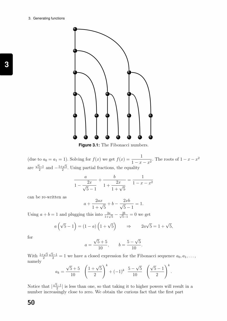
3


Figure 3.1: The Fibonacci numbers.

(due to a0 = a1 = 1). Solving for f(x) we get f(x) =1

1− x− x2 . The roots of 1− x− x2

are√5−12

and −1+√5

2. Using partial fractions, the equality

a

1− 2x√5− 1

+b

1 +2x

1 +√

5

=1

1− x− x2

can be re-written as

a+2ax

1 +√

5+ b− 2xb√

5− 1= 1.

Using a+ b = 1 and plugging this into 2a1+√5− 2b√

5−1 = 0 we get

a(√

5− 1)

= (1− a)(

1 +√

5)

⇒ 2a√

5 = 1 +√

5,

for

a =

√5 + 5

10, b =

5−√

5

10.

With 1+√5

2

√5−12

= 1 we have a closed expression for the Fibonacci sequence a0, a1, . . . ,namely

ak =

√5 + 5

10

(1 +√

5

2

)k

+ (−1)k5−√

5

10

(√5− 1

2

)k

.

Notice that |√5−12| is less than one, so that taking it to higher powers will result in a

number increasingly close to zero. We obtain the curious fact that the first part

50

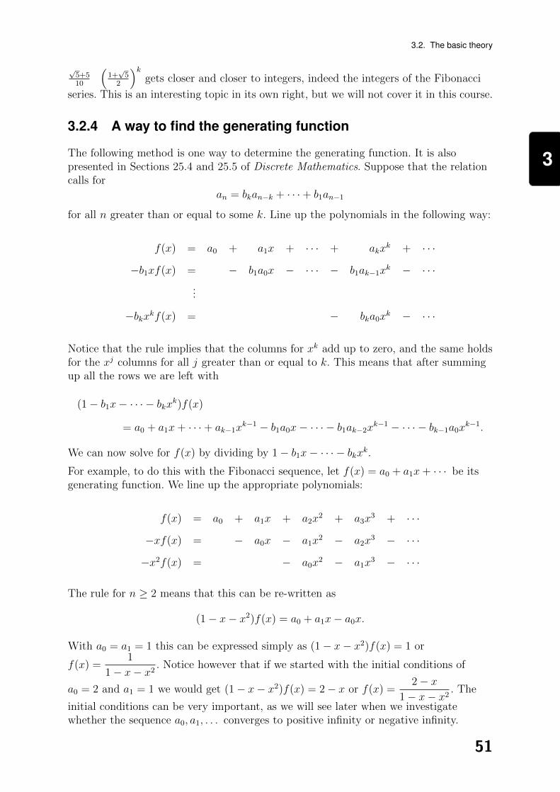
3


√5+510

(1+√5

2

)kgets closer and closer to integers, indeed the integers of the Fibonacci

series. This is an interesting topic in its own right, but we will not cover it in this course.

3.2.4 A way to find the generating function

The following method is one way to determine the generating function. It is alsopresented in Sections 25.4 and 25.5 of Discrete Mathematics. Suppose that the relationcalls for

an = bkan−k + · · ·+ b1an−1

for all n greater than or equal to some k. Line up the polynomials in the following way:

f(x) = a0 + a1x + · · · + akxk + · · ·

−b1xf(x) = − b1a0x − · · · − b1ak−1xk − · · ·...

−bkxkf(x) = − bka0xk − · · ·

Notice that the rule implies that the columns for xk add up to zero, and the same holdsfor the xj columns for all j greater than or equal to k. This means that after summingup all the rows we are left with

(1− b1x− · · · − bkxk)f(x)

= a0 + a1x+ · · ·+ ak−1xk−1 − b1a0x− · · · − b1ak−2xk−1 − · · · − bk−1a0xk−1.

We can now solve for f(x) by dividing by 1− b1x− · · · − bkxk.For example, to do this with the Fibonacci sequence, let f(x) = a0 + a1x+ · · · be itsgenerating function. We line up the appropriate polynomials:

f(x) = a0 + a1x + a2x2 + a3x

3 + · · ·

−xf(x) = − a0x − a1x2 − a2x

3 − · · ·

−x2f(x) = − a0x2 − a1x

3 − · · ·

The rule for n ≥ 2 means that this can be re-written as

(1− x− x2)f(x) = a0 + a1x− a0x.

With a0 = a1 = 1 this can be expressed simply as (1− x− x2)f(x) = 1 or

f(x) =1

1− x− x2 . Notice however that if we started with the initial conditions of

a0 = 2 and a1 = 1 we would get (1− x− x2)f(x) = 2− x or f(x) =2− x

1− x− x2 . The

initial conditions can be very important, as we will see later when we investigatewhether the sequence a0, a1, . . . converges to positive infinity or negative infinity.

51

3


3.2.5 Algebraic manipulations

The following algebraic manipulations of generating functions are presented in Sections25.1 and 25.2 of Discrete Mathematics and Section 4.2 of Combinatorics.

With any integer k , positive, negative, or zero, a sequence akxk + ak+1x

k+1 + · · · iscalled a Laurent series. Usually we are interested in the Laurent series that start withnon-negative k, otherwise known as power series. One can add and subtract any pair ofLaurent series, each position separately. By starting at the lowest power and followinginductively, always adding together only finitely many terms, one can multiply togethertwo Laurent series. For example, if the two series start with x4 + 2x6 + · · · and2x−1 + 3x+ · · · we know that the product of the two series will look like 2x3 + 7x5 + · · ·(from the information given we do not know the rest of the coefficients).

With the same kind of approach, given any Laurent series f = aixi + ai+1x

i+1 + · · · that

is not zero, with ai 6= 0, we can find its multiplicative inverse1

f. We start with the

leading coefficient b−i =1

ai. We multiply b−ix−i with f to get

1 + b−iai+1x1 + b−iai+2x

2 + · · · .

We look for the appropriate coefficient b−i+1 for x−i+1 so that the x1 coefficientdisappears. The right choice for b−i+1 satisfies

b−i+1ai + b−iai+1 = 0.

Since ai is not zero there is a unique solution for b−i+1. Proceeding in this way we canfind the Laurent series

1

f= b−ix

−i + b−i+1x−i+1 + · · ·

such that when multiplied with f the result is 1. Another way to express1

f(x)is

f−1(x). Next, we can perceive the expressionf(x)

g(x)as f(x)g−1(x), the product of two

Laurent series.

To illustrate this, let f(x) = 1− x+ 2x2 − 3x3 + 4x4 − · · · . We see that

(1 + x)(1− x+ 2x2 − 3x3 + 4x4 − . . . ) = 1 + x2 − x3 + x4 + . . . .

This suggests that the next polynomial to try is (1 + x− x2), and indeed we get

(1 + x− x2)(1− x+ 2x2 − 3x3 + 4x4 − · · · ) = 1− x4 + · · · ,

with the next approximation 1 + x− x2 + x4.

An explicit method for finding1

fis called long division and can be performed with

polynomials in the same way as it is done with integers. We return to this method later.

Another algebraic method that is very useful for analysing generating functions is thatof partial fractions, also presented in Section 25.2 of Discrete Mathematics. Given the

52

3


expressionf(x)

g(x)where the degree of f(x) is strictly less than the degree of g(x) and

g(x) can be factored into gn11 (x) · · · gnl

l (x) we can re-writef(x)

g(x)as a sum of terms of the

formr

gkj (x)where r is a number and k is no greater than nj. The same method is used

to help integrate such functions. For example, suppose we have the generating function

x2 − 2x− 1

1− x− x2 + x3.

First notice that 1− x− x2 + x3 is equal to (1− x)2(1 + x). So we can re-write:

x2 − 2x− 1

1− x− x2 + x3=

a

(1− x)2+

b

1− x +c

1 + x.

Multiplying through by 1− x− x2 + x3 we get

x2 − 2x− 1 = a(1 + x) + b(1 + x)(1− x) + c(1− x)2.

We could collect like powers of x and solve for three linear equations in three unknowns.But the easier way is through the cover-up rule. Choose three distinct values for x thatmake the calculations easy. Two of these choices are obvious, x = 1 and x = −1. Fromx = 1 we get 1− 2− 1 = 2a, or a = −1. From x = −1 we get 1 + 2− 1 = 4c, or c = 1

2.

For a third choice x = 0 is possible, and with a and c already solved we get−1 = −1 + b+ 1

2or b = −1

2. Therefore

x2 − 2x− 1

1− x− x2 + x3= − 1

(1− x)2− 1

2(1− x)+

1

2(1 + x).

Why does the cover-up rule work? With the above example, we have to solve for

x2 − 2x− 1 = a(1 + x) + b(1 + x)(1− x) + c(1− x)2,

or in other words we had two polynomials of degree 2 which had to be equal. Touniquely determine a polynomial f(x) of degree n or less it suffices to know its valuesfor n+ 1 distinct values of x. Let us assume that there is a second polynomial g ofdegree n or less that agrees with f on these n+ 1 distinct values of x. That would meanthat f − g, a polynomial of degree n or less, has n+ 1 distinct roots. This is possibleonly if f − g = 0, meaning f = g. The formal argument for why a polynomial of degreen cannot have more than n distinct roots is presented in a later chapter.

3.2.6 Calculus manipulations

Taking derivatives of generating functions and its applications are presented in Section4.2 of Combinatorics and in Exercise 25.7 of Discrete Mathematics.

One can take the derivative of any Laurent series, using the rule that the derivative ofxn is nxn−1, also when n is negative. Many of the other rules of calculus apply. We

demonstrate by taking the derivative of1

1− x = 1 + x+ x2 + · · · .

53

3


The derivative of the left side is1

(1− x)2and on the right side it is

1 + 2x+ 3x2 + 4x3 + · · · .

We continue this process. The derivative of x−n is −nx−n−1 for all n = 1, 2, 3, . . . ,meaning that the derivative of (1− x)−n is n(1− x)−n−1. Taking the derivatives of bothsides (the second time) we get

2

(1− x)3= 2 + 3 · 2x+ 4 · 3x2 + 5 · 4x3 + · · · ,

which is better formulated as

1

(1− x)3= 1 +

(3

2

)x+

(4

2

)x2 +

(5

2

)x3 + · · · .

Differentiating both sides of the expression for2

(1− x)3we get

6

(1− x)4= 3 · 2 + 4 · 3 · 2x+ 5 · 4 · 3x2 + · · ·

which we can rewrite as

1

(1− x)4= 1 +

(4

3

)x+

(5

3

)x2 + · · · .

The following is Theorem 25.3 of Discrete Mathematics.

Lemma 3.1 Assume that1

(1− x)n= a0 + a1x+ a2x

2 + · · · . Then the coefficients ak

are equal to

(k + n− 1

k

).

Proof (1)We proceed by induction. If n = 1 then all these coefficients should be 1, since

1 + x+ x2 + · · · = 1

1− x . And indeed

(k + 1− 1

k

)is equal to 1.

Assume the formula is true for n− 1 for any given n ≥ 2. Write

(1− x)−n+1 ≡ 1

(1− x)n−1= a0 + a1x+ a2x

2 + · · ·

and1

(1− x)n= b0 + b1x+ b2x

2 + · · · .

We take the derivative of both sides of the equation (1− x)−n+1 to get

n− 1

(1− x)n= a1 + 2a2x+ 3a3x

2 + · · · .

Bringing in the bi coordinates,

(n− 1)b0 + (n− 1)b1x+ · · · = a1 + 2a2x+ · · · ,

54

3


or (n− 1)bi = (i+ 1)ai+1 for all i ≥ 0.

With the induction assumption, we have

(n− 1)bi = (i+ 1)

((n− 1) + (i+ 1)− 1

i+ 1

).

Solving for bi we get

bi =(i+ 1)(i+ n− 1)!

(i+ 1)!(n− 2)!(n− 1)=

(n+ i− 1

i

).

Proof (2)Notice that the coefficient for xk of the power series (1 + x+ x2 + · · · )n is the number ofways to select with repetition n positions for k unordered objects, which we knew

already to be

(n− 1 + k

k

).

Return to generating functions a0 + a1x+ · · · of the form1

(1− x)n, which have a

solution of ak =

(n− 1 + k

k

). For any fixed n ≥ 1 re-write

(n− 1 + k

k

)as

1

(n− 1)!(k + 1)(n−1), a polynomial in k of degree n− 1. Let us look at the polynomials

1

(n− 1)!(x+ 1)(n−1).

n = 1 :1

0!(x+ 1)(0) = 1

n = 2 :1

1!(x+ 1)(1) = x+ 1

n = 3 :1

2!(x+ 1)(2) =

1

2(x+ 2)(x+ 1) =

x2 + 3x+ 2

2

n = 4 :1

3!(x+ 1)(3) =

1

6(x+ 3)(x+ 2)(x+ 1) =

x3 + 6x2 + 11x+ 6

6.

These polynomials form a basis of the space of polynomials in x. Therefore anypolynomial can be written as a linear combination of them. In this way we can find thegenerating functions for any sequences defined by an = nk for any positive integer k,

since we know from Lemma 3.1 that the generating function for bn =

(n− 1 + k

k

)is

1

(1− x)k= b0 + b1x+ · · · .

Assume that c is any non-zero complex number and make the substitution y = cx. We

get that the generating function a0 + a1x+ · · · for an =

(n− 1 + k

k

)cn is

1

(1− cx)k.

For the same reason as above we can find the algebraic expression for the generatingfunction a0 + a1x+ · · · for any sequence defined by an = nkcn.

55

3


3.2.7 How to find the explicit solution

Putting together what we have learned so far, we discover a method for going from agenerating function to the explicit formula for its coefficients. There is, however, aproblem with this method, discussed later, which may make it impractical in manysituations.

First, put it in the form of h(x) +f(x)

g(x)such that the degree of f(x) is less than the

degree of g(x) and g(0) is equal to 1.

Second, express g(x) as a product of irreducible factors. Using complex numbers, anypolynomial can be factored down completely to

∏k(x− ri)mk where the rk are the roots

of the polynomial (with multiplicities mk) and∑

kmk is the degree of the polynomial.For example, x2 + 1 is irreducible over the real numbers, but with complex numbersx2 + 1 = (x+ i)(x− i), where i is the square root of −1. This is the hardest part of thetechnique, since finding exact expressions for these roots may be impossible. However, ifapproximate values are sufficient, then this method works. Given that g(0) = 1 we can

express g(x) as∏

k

(1− x

rk

)mk

, where rk are the roots.

Third, with g(x) factored and expressed as∏

k

(1− x

rk

)mk

, one applies the methods of

partial fractions and solves for the unique (complex) numbers bk,j which satisfy

f(x)

g(x)=∑

k

mk∑

j=1

bk,j(1− x

rk

)j .

Fourth, one uses Lemma 3.1 to express the pth power coefficient of f(x)/g(x) as

∑

k

mk∑

j=1

bk,j

(1

rk

)p(p+ j − 1

p

).

Fifth, combine with the polynomial h(x) (determining the initial values of the sequence)for the complete answer.

A second approach to giving change

First, let us stick to giving change in only one and two pence coins, since otherwise theexplicit approach could be difficult. We want to know the coefficients of the power series

1

(1− x)(1− x2) . Since 1− x2 = (1− x)(1 + x) this should be expressed as

1

(1− x)2(1 + x). Using partial fractions write this as

a

1− x +b

(1− x)2+

c

1 + x=

1

(1− x)2(1 + x).

Re-write it as(1− x)(1 + x)a+ (1 + x)b+ (1− x)2c = 1

56

3


and again as(c− a)x2 + (b− 2c)x+ a+ b+ c = 1.

We use the cover-up rule with x = 0, 1,−1:2b = 14c = 1a+ b+ c = 1.

The solution is a = 14, b = 1

2, and c = 1

4. (The cover-up rule will be explained later.)

The power series for1

1− x and1

1 + xare not difficult. We are already familiar with

1

1− x = 1 + x+ x2 + · · · ,

while1

1 + x= 1− x+ x2 − x3 + x4 − · · · .

Therefore the sum of1

4(1− x)and

1

4(1 + x)is easy to express. At even positions we get

1

2and at odd positions we get 0. The

1

2(1− x)2is more difficult to understand.

The derivative of the function1

1− x is1

(1− x)2. Therefore we get

1

(1− x)2= 1 + 2x+ 3x2 + 4x3 + · · ·

Now we can say explicitly how many ways one can give n pence in change using onlyone or two pence coins. For any n we add half of n+ 1 to the previous result (addingthe two easier power series) to get

if n is odd, inn+ 1

2ways

if n is even, inn+ 2

2ways.

This corresponds exactly to our previous table. Needless to say, making the sameexplicit calculation for coins in one, two, and five pence would be significantly moredifficult using this method. For all k ≥ 2 some of the roots of the polynomials1 + x+ · · ·+ xk are non-real complex numbers (the roots of unity). Using tables is aneasier method when there are coins of higher value. However we extend this approach tocoins to the value of one and four (though a four pence coin does not exist).

Giving change in one and four pence coins

Given that there exists a four pence coin, we work through the explicit solution usingcomplex numbers. We take advantage of the fact that i and −i are also fourth roots ofone. Notice from the solution that working this out for five pence coins would beconsiderably more difficult, though it would not be too difficult to extend this methodto one, two, and four pence coins.

57

3


The generating function is1

1− x1

1− x4 .

The roots of x4 − 1 are 1, −1, i, and −i (with i and −i the complex numbers such thati2 = −1). The generating function can be re-written as

1

(1− x)21

1 + x

1

1− ix1

1 + ix.

Breaking down into partial fractions with variables a, b, c, d, e to solve we get thegenerating function equal to

a

1 + ix+

b

1− ix +c

1 + x+

d

1− x +e

(1− x)2.

The equation can be re-written again as

1 = (1− x)2(1− ix)(1 + x)a+ (1− x)2(1 + ix)(1 + x)b

+ (1 + x2)(1− x)2c+ (1 + x2)(1− x)(1 + x)d+ (1 + x2)(1 + x)e.

Using the cover-up rule with x = i,−i, 1,−1, 0:

x = 1 : 4e = 1

x = −1 : 8c = 1

x = i : 4(1− i)a = 1

x = −i : 4(i+ 1)b = 1

x = 0 : a+ b+ c+ d+ e = 1

This solves to yield

a =1

8+

1

8i, b =

1

8− 1

8i, c =

1

8, d =

3

8, e =

1

4.

The formula for the kth coordinate of the generating function is therefore(

1

8− 1

8i

)ik +

(1

8+

1

8i

)(−i)k +

1

8(−1)k +

3

8+

1

4(k + 1).

Let us check a few values.

a0 =1

8+

1

8i+

1

8− 1

8i+

1

8+

3

8+

1

4= 1

a1 =1

8i+

1

8− 1

8i+

1

8− 1

8+

3

8+

1

2= 1

a2 = −1

8− 1

8i− 1

8+

1

8i+

1

8+

3

8+

3

4= 1

a3 =1

8i− 1

8− 1

8i− 1

8− 1

8+

3

8+ 1 = 1

a4 =1

4+

1

8+

3

8+

5

4= 2

58

3

3.3. Recurrence relations


Exercise 3.1

Find the generating function for the sequence an = 2nn2. Hint: Look at the solutions to

the generating functions1

(1− 2x)kand the fact that n2 can be written in terms of

(n

2

),

n and 1.

Exercise 3.2

An eccentric professor climbs stairs by taking either two stairs or one stair in one stride.Find a formula for bn, the number of ways in which he can climb n stairs (and the threesolutions 1 + 2 + 2, 2 + 1 + 2 and 2 + 2 + 1 are all distinct).

Exercise 3.3

Find the explicit solution for the coefficients of the generating function1

1 + x+ x2using

complex numbers. Hint: Use that x3 − 1 = (x− 1)(x2 + x+ 1).

Exercise 3.4

What is the generating function for the number of ways to distribute k pence to threepeople (distinguishable) in one, two, and five pence coins so that the first person nevergets a one-pence (penny) coin, the second person never gets a two-pence coin, and thethird person never gets a five-pence coin?

3.3 Recurrence relations

3.3.1 What is a recurrence relation?

Recurrence relations are introduced with generating functions at the start of Chapter 4of Combinatorics in the following way: ‘A recurrence relation expresses the value of afunction f at the natural number n in terms of its values at smaller natural numbers.’

Let N = {0, 1, 2, . . . }, the natural numbers, be the non-negative integers and Z be allintegers. Sometimes a definition of a recurrence relation is given as follows.

A recurrence relation of degree k is defined by a function p : N× Zk → Z and an initialsequence of integers a0, a1, a2, . . . , ak−1 such that for all n ≥ k the number an is equal top(n, an−1, . . . , an−k).

The problem with this definition is that it describes any function on the natural numberif there is no restriction on the properties of the function p. But usually some form ofrestriction on p is implicit in this definition.

A linear recurrence of degree k is defined by a function p such that for all n ≥ k

p(n, x1, . . . , xk) = q(n) + b1xn−1 + · · ·+ bkxn−k

for some function q and constants b1, b2, . . . , bk.

It is homogeneous if the function q is the zero function.

59

3


The homogeneous linear recurrence relations have a special structure that we will studyin some depth. And their definition as stated above is not ambiguous.

Just as recurrence relations define generating functions, so one can move in the oppositedirection.

Example 3.1 Let

f(x) =1 + 7x

1 + x− 6x2

and now determine the recursive relation for which f(x) is the generating function.Then determine the explicit formula for ai as well as the initial values a0 and a1.

Due to the polynomial in the denominator and our previous analysis of how to gofrom the recurrence relation to the generating function, we have for n ≥ 2an = −an−1 + 6an−2. The initial conditions are a0 = 1 and a1 = 6 (seen from theinitial process of long division). With 1 + x− 6x2 = (1− 2x)(1 + 3x) we can write

1 + 7x

1 + x− 6x2=

a

1− 2x+

b

1 + 3x

or (1 + 3x)a+ (1− 2x)b = 1 + 7x. With the cover-up rule, letting x = 12

we get a = 95

and with x = −13

we get b = −45

. This solves to an = 952n − 4

5(−3)n.

Checking this on n = 2, 3, 4, 5 by the recursive formula we get a2 = 0, a3 = 36,a4 = −36, and a5 = 7 · 36 = 252 = 4

5243 + 9

532.

3.3.2 Equivalences

Putting together everything we have learned so far, we can characterise homogeneouslinear recurrence relationships in terms of their generating functions.

Define a generating function to be rational if it can be expressed as a fraction of onepolynomial over another. This follows the definition of a rational number being aninteger divided by a non-zero integer.

Lemma 3.2 A rational generating function defines a homogeneous linear recurrencerelation. Furthermore if a recurrence relation is linear and the function q(n) has arational generating function then the generating function of the recurrence relation isalso rational.

ProofAssume that f(x) is the generating function for the sequence a0, a1, . . . . Assume that

f(x) =g(x)

h(x)with h(x) = ckx

k + · · ·+ c0 a polynomial of degree k and

g(x) = blxl + · · ·+ b0 a polynomial of degree l. Re-write as h(x)f(x) = g(x). Let i be the

first number such that ci is not zero.

(ckxk + · · ·+ cix

i)(a0 + a1x+ · · · ) = blxl + · · ·+ b0.

Assuming j > max{l, k} and looking at the (j + i)th coefficient we have

ajci + aj−1ci+1 + · · ·+ aj−k+ick = 0.

60

3


With ci not equal to zero, divide by ci and solve for aj for

aj = −ci+1

ciaj−1 − · · · −

ckciaj−k+i.

For the second part, let g(x) = q(k)xk + q(k + 1)xk+1 + · · · be the generating functionfor the function q. Look at the function

h(x) := f(x)(1− b1x− b2x2 − · · · − bkxk)− g(x),

where the b1, b2, . . . , bk define the recurrence relation. For all j ≥ k the xj coefficient isaj − b1aj−1 − · · · − bkaj−k − q(j), which is zero by assumption. Therefore h(x) is apolynomial of degree at most k − 1. We can re-write f(x) as

h(x) + g(x)

1− b1x− b2x2 − · · · − bkxk.

Theorem 3.3 The following are equivalent about an infinite sequence a0, a1, . . . :

(i) The sequence is determined by a homogeneous linear recurrence relation.

(ii) The expression a0 + a1x+ a2x2 + · · · is a rational generating function(

f

gfor some polynomials f, g with g 6= 0

).

(iii) There is a positive integer t such that for all k ≥ t

ak =n∑

p=1

mp∑

j=0

bp,j (1

rp)kkj

for some fixed n, m1, . . .mn, complex numbers b1,1, . . . , b1,m1 , b2,1, . . . , bn,mn andcomplex numbers r1, . . . , rn.

If so then the r1, . . . , rn are the roots of g(x) such that the generating function reduces

tof(x)

g(x)for polynomials f(x), g(x).

ProofThe equivalency of (i) and (ii) is Lemma 3.2 . (ii) implies (iii) is the result of ourexplicit solution for the series. (iii) implies (ii) results from the fact that

1

(n− 1)![k + 1]n−1 =

(n− 1 + k

k

), the explicit solutions an for the generating function

∑∞n=0 any

n =1

(1− y)k, for n = 1, 2, . . . form a basis of the polynomials in k, as

described above.

Notice that y = rx can be substituted to incorporate the powers of 1r

and that shifts ofindex can be rewritten without the shift, such as an = (n− 1)2 re-written asan = n2 − 2n+ 1 or an = cn+1 as an = c · cn. (i) implies (iii) of the above is alsoTheorem 25.5.2 of Discrete Mathematics.

61

3


3.3.3 Tables and long division

Theoretically we know how to write down closed-form formulae for the recurrencerelations defined by all rational generating functions. But in reality finding the complexroots of the appropriate polynomial may be too difficult, if not impossible. Given thatonly partial factorisation of the polynomial in the denominator is possible, sometimes atable of solutions is all that one can hope for.

As with the tables created for giving change in different types of coins, we can constructsequences of solutions in tables, where the last sequence is the recurrence relationdesired. The general approach is the following. Start with a rational generating function

h(x) +f(x)

g1(x)g2(x) · · · gm(x)

where for all i gi(0) = 1 and the gi cannot be factored further and the degree of f is lessthan the sums of the degrees of the gi.

For every i = 1, 2, . . .m define the generating function ji to bef(x)

g1(x) · · · gi(x), so that

g1(x)j1(x) = f(x) and gi(x)ji(x) = ji−1(x).

Let

gi(x) = 1 + bi,1x+ bi,2x2 + bi,pix

pi ,

f(x) = f0 + f1x+ · · ·+ flxl,

jr(x) = ar,0 + ar,1x+ ar,2x2 + · · · .

For the first line of the table write down the finite sequence

f0 f1 . . . fl

For any given k look at the coefficient for xk in the expression g1(x)j1(x) = f(x)

(1 + b1,1x+ b1,2x2 + b1,p1x

p1)(a1,0 + a1,1x+ a1,2x2 + · · · ) = f0 + f1x+ · · ·+ flx

l.

We get a1,0 = f0 anda1,k = fk − b1,1a1,k−1 − · · · − b1,ka1,0,

with fk = 0 if k > l.

The sequence for j1 can be written down according to this rule, below the sequencef0, . . . , fl.

f0 f1 . . . fl

a1,0 a1,1 . . . a1,l . . .

Assuming that this has been done for j1, j2, . . . , jr−1, we create the sequencear,0, ar,1, . . . corresponding to the generating function jr. With gr(x)jr(x) = jr−1(x) wedo the same trick:

(1 + br,1x+ br,2x2 + br,prx

pr)(ar,0 + ar,1x+ ar,2x2 + · · · ) = ar−1,0 + ar−1,1x+ · · ·

62

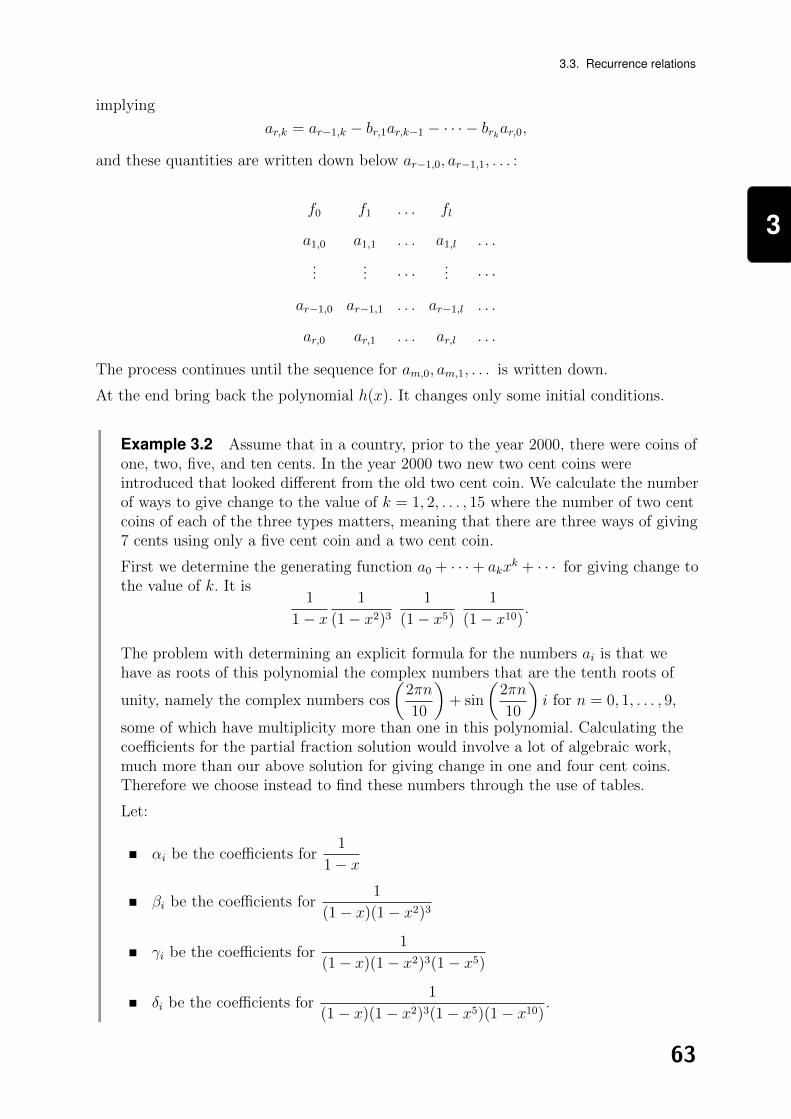
3


implying

ar,k = ar−1,k − br,1ar,k−1 − · · · − brkar,0,

and these quantities are written down below ar−1,0, ar−1,1, . . . :

f0 f1 . . . fl

a1,0 a1,1 . . . a1,l . . .

...... · · · ... · · ·

ar−1,0 ar−1,1 . . . ar−1,l . . .

ar,0 ar,1 . . . ar,l . . .

The process continues until the sequence for am,0, am,1, . . . is written down.

At the end bring back the polynomial h(x). It changes only some initial conditions.

Example 3.2 Assume that in a country, prior to the year 2000, there were coins ofone, two, five, and ten cents. In the year 2000 two new two cent coins wereintroduced that looked different from the old two cent coin. We calculate the numberof ways to give change to the value of k = 1, 2, . . . , 15 where the number of two centcoins of each of the three types matters, meaning that there are three ways of giving7 cents using only a five cent coin and a two cent coin.

First we determine the generating function a0 + · · ·+ akxk + · · · for giving change to

the value of k. It is1

1− x1

(1− x2)31

(1− x5)1

(1− x10) .

The problem with determining an explicit formula for the numbers ai is that wehave as roots of this polynomial the complex numbers that are the tenth roots of

unity, namely the complex numbers cos

(2πn

10

)+ sin

(2πn

10

)i for n = 0, 1, . . . , 9,

some of which have multiplicity more than one in this polynomial. Calculating thecoefficients for the partial fraction solution would involve a lot of algebraic work,much more than our above solution for giving change in one and four cent coins.Therefore we choose instead to find these numbers through the use of tables.

Let:

αi be the coefficients for1

1− x

βi be the coefficients for1

(1− x)(1− x2)3

γi be the coefficients for1

(1− x)(1− x2)3(1− x5)

δi be the coefficients for1

(1− x)(1− x2)3(1− x5)(1− x10) .

63

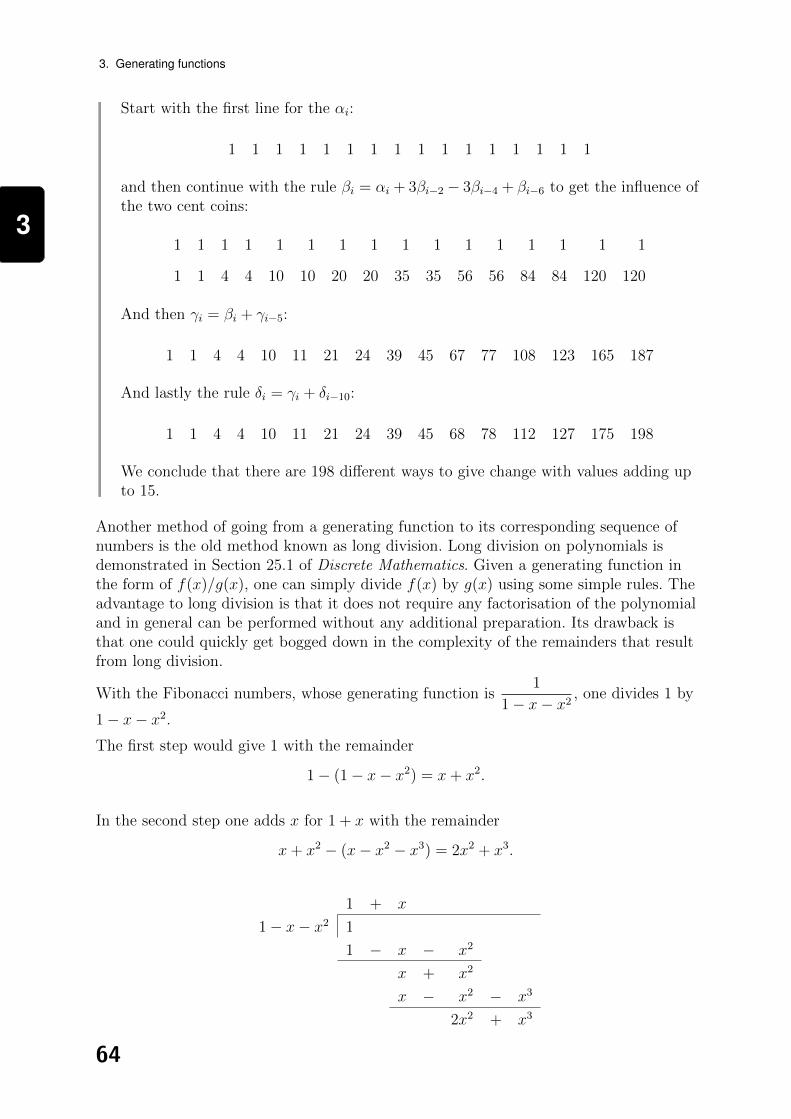
3


Start with the first line for the αi:

1 1 1 1 1 1 1 1 1 1 1 1 1 1 1 1

and then continue with the rule βi = αi + 3βi−2 − 3βi−4 + βi−6 to get the influence ofthe two cent coins:

1 1 1 1 1 1 1 1 1 1 1 1 1 1 1 1

1 1 4 4 10 10 20 20 35 35 56 56 84 84 120 120

And then γi = βi + γi−5:

1 1 4 4 10 11 21 24 39 45 67 77 108 123 165 187

And lastly the rule δi = γi + δi−10:

1 1 4 4 10 11 21 24 39 45 68 78 112 127 175 198

We conclude that there are 198 different ways to give change with values adding upto 15.

Another method of going from a generating function to its corresponding sequence ofnumbers is the old method known as long division. Long division on polynomials isdemonstrated in Section 25.1 of Discrete Mathematics. Given a generating function inthe form of f(x)/g(x), one can simply divide f(x) by g(x) using some simple rules. Theadvantage to long division is that it does not require any factorisation of the polynomialand in general can be performed without any additional preparation. Its drawback isthat one could quickly get bogged down in the complexity of the remainders that resultfrom long division.

With the Fibonacci numbers, whose generating function is1

1− x− x2 , one divides 1 by

1− x− x2.The first step would give 1 with the remainder

1− (1− x− x2) = x+ x2.

In the second step one adds x for 1 + x with the remainder

x+ x2 − (x− x2 − x3) = 2x2 + x3.

1 + x

1− x− x2 1

1 − x − x2

x + x2

x − x2 − x3

2x2 + x3

64

3


In the third step one adds 2x2 for 1 + x+ 2x2 and the remainder

2x2 + x3 − (2x2 − 2x3 − 2x4) = 3x3 + 2x4.

In the fourth step one adds 3x3 for 1 + x+ 2x2 + 3x3 with the remainder

3x3 + 2x4 − (3x3 − 3x4 − 3x5) = 5x4 + 3x5.

The next step yields a 5x4. One recognises the pattern of the Fibonacci sequence in theprocess of this long division.

3.3.4 Composite linear recurrence relations

The relationship between many homogeneous linear recurrence relations and theirgenerating functions can be well disguised. For example, for every n we may define ldifferent types of objects such that the number an of objects we want to know is thesum of the numbers of the different types. The relations could be expressed entirely interms of these different types, so that the relation between the an and the previousan−1, an−2, . . . is obscured. How could we discover the formula that makes it ahomogeneous linear recurrence relation? Formally we have for all n ≥ k

bjn =n∑

i=1

l∑

j=1

pji bjn−i

for some variables pji and initial values b10, . . . , bl0, . . . , b1k−1, . . . , blk−1.

Often cleverness suffices to discover the general pattern without the complexity of acomposite formulation. For example, if an stands for the number of ways to climb nstairs with strides of length 1, 2, or 3 one should recognise that an = an−1 + an−2 + an−3(from the last step being of size one, two, or three) without defining an additional threesequences bn, cn, and dn, representing the ways to end in strides of length 1, 2, and 3respectively.

It is good to know, however, that failing some clever solution to the problem that thereis a general method of linear algebra that will work.

Example 3.3 To demonstrate this method, we define a0 = 1, b0 = 0, c0 = 0, andfor all i ≥ 1 by

ai = ci−1 + bi−1 + ai−1,

bi = ai−1 − ci−1,

ci = ai−1 − bi−1,and we want to know ai for all i ≥ 0.

Let f , g, and h be the generating functions for the ai, bi, and ci. We have

f = 1 + xg + xh+ xf,

g = xf − xh,

h = xf − xg.

65

3


We can treat f , g, and h as variables, place these relations in a matrix, and solveusing the techniques of linear algebra:

x− 1 x x

−x 1 x

−x x 1

f

g

h

=

−1

0

0

which reduces to

x2 + x− 1 0 x− x2

−x 1 x

1 0 −x+ 1

x

f

g

h

=

−1

0

0

and

0 0 1

0 1 −1

1 0 −x+ 1

x

f

g

h

=

x

1− 3x2

0

0

and solves to

f =1 + x

1− 3x2, g = h =

x

1− 3x2.

Now solve for an with

u

1−√

3x+

v

1 +√

3x=

1 + x

1− 3x2

thus

(1 +√

3x)u+ (1−√

3x)v = 1 + x.

Using the cover-up rule with x =√33,−√33

we get u =√3+36

and v = 3−√3

6for

ak =

√3 + 3

6(√

3)k +3−√

3

6(−√

3)k

This corresponds to the answers obtained directly: a0 = 1, b0 = c0 = 0,a1 = b1 = c1 = 1, a2 = 3, b2 = c2 = 0, a3 = 3.

3.3.5 Initial conditions

Two recurrence relations, both ruled by the same formula an = b1an−1 + · · ·+ bkan−k forall n ≥ k, can act very differently. To illustrate this, we look at simple recurrencerelations defined by integers such that the initial conditions can determine whether the

66

3


series goes to positive infinity or negative infinity.

Example 3.4 Define a recurrence relation by

α0 = 1, αn = 3αn−1 − 2αn−2 − n,

for all n ≥ 2, with α1 a variable.

Try first α1 = 1:

α0 = 1,

α1 = 1,

α2 = 3− 2− 2 = −1,

α3 = −3− 2− 3 = −8,

and so on downward.

Next try α1 = 3:

α0 = 1,

α1 = 3,

α2 = 9− 2− 2 = 5,

α3 = 15− 6− 3 = 6,

α4 = 18− 10− 4 = 4,

α5 = 12− 12− 5 = −5.

Next try α1 = 4:

α0 = 1,

α1 = 4,

α2 = 12− 2− 2 = 8,

α3 = 24− 8− 3 = 13.

Will this continue going up, or fall back like the others?

Let f(x) be the generating function for α0, α1, . . . .

With1

(1− x)2equal to 1 + 2x+ 3x2 + · · · it follows that

x

(1− x)2is the generating

function for the recurrence relation αn = n. We assume that α1 = 4

f(x) = 1 + 4x + α2x2 + α3x

3 + · · ·

−3xf(x) = − 3x − 12x2 − 3α2x3 − · · ·

+2x2f(x) = + 2x2 + 8x3 + · · ·

+x

(1− x)2= + x + 2x2 + 3x3 + · · · .

67

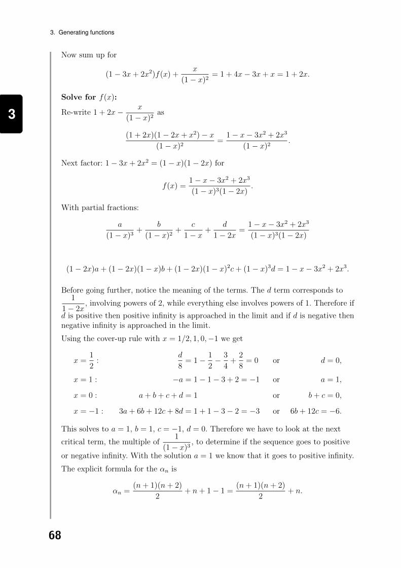
3


Now sum up for

(1− 3x+ 2x2)f(x) +x

(1− x)2= 1 + 4x− 3x+ x = 1 + 2x.

Solve for f(x):

Re-write 1 + 2x− x

(1− x)2as

(1 + 2x)(1− 2x+ x2)− x(1− x)2

=1− x− 3x2 + 2x3

(1− x)2.

Next factor: 1− 3x+ 2x2 = (1− x)(1− 2x) for

f(x) =1− x− 3x2 + 2x3

(1− x)3(1− 2x).

With partial fractions:

a

(1− x)3+

b

(1− x)2+

c

1− x +d

1− 2x=

1− x− 3x2 + 2x3

(1− x)3(1− 2x)

(1− 2x)a+ (1− 2x)(1− x)b+ (1− 2x)(1− x)2c+ (1− x)3d = 1− x− 3x2 + 2x3.

Before going further, notice the meaning of the terms. The d term corresponds to1

1− 2x, involving powers of 2, while everything else involves powers of 1. Therefore if

d is positive then positive infinity is approached in the limit and if d is negative thennegative infinity is approached in the limit.

Using the cover-up rule with x = 1/2, 1, 0,−1 we get

x =1

2:

d

8= 1− 1

2− 3

4+

2

8= 0 or d = 0,

x = 1 : −a = 1− 1− 3 + 2 = −1 or a = 1,

x = 0 : a+ b+ c+ d = 1 or b+ c = 0,

x = −1 : 3a+ 6b+ 12c+ 8d = 1 + 1− 3− 2 = −3 or 6b+ 12c = −6.

This solves to a = 1, b = 1, c = −1, d = 0. Therefore we have to look at the next

critical term, the multiple of1

(1− x)3, to determine if the sequence goes to positive

or negative infinity. With the solution a = 1 we know that it goes to positive infinity.

The explicit formula for the αn is

αn =(n+ 1)(n+ 2)

2+ n+ 1− 1 =

(n+ 1)(n+ 2)

2+ n.

68

3


Check how it continues, as we have already calculated α2 = 8 and α3 = 13. On theleft side is the explicit formula, on the right side the numbers are from therecurrence relation:

α4 =5 · 6

2+ 4 = 19 = 3 · 13− 2 · 8− 4

α5 =6 · 7

2+ 5 = 26 = 3 · 19− 2 · 13− 5.

What if α1 = 3 or α1 = 5? The main equation is

(1− 3x+ 2x2)f(x) +x

(1− x)2= 1 + α1x− 3x+ x.

If α1 = 3 the right side is 1 + x.

If α1 = 5 the right side is 1 + 3x.

For α1 = 3 we get the explicit solution

αn =(n+ 1)(n+ 2)

2+ n+ 1− 2n,

and for α1 = 5 we get the explicit solution

αn =(n+ 1)(n+ 2)

2+ n− 1 + 2n.

Example 3.5 Let the recurrence relation be defined by a0 = 1 and for n ≥ 2

αn = 3αn−1 − 2αn−2 − 5n.

For what values of α1 will the limit of the sequence be positive infinity?

f(x) = 1 + α1x + α2x2 + α3x

3 + · · ·

−3xf(x) = − 3x − 3α1x2 − 3α2x

3 − · · ·

+2x2f(x) = + 2x2 + 2α1x3 + · · ·

+5x

(1− x)2= + 5x + 10x2 + 15x3 + · · ·

Sum up for

(1− 3x+ 2x2)f(x) +5x

(1− x)2= 1 + α1x+ 2x

and

f(x) =1 + α1x− 5x− 3x2 − 2α1x

2 + 2x3 + α1x3

(1− x)3(1− 2x).

Putting into partial fractions:

a

(1− x)3+

b

(1− x)2+

c

1− x +d

1− 2x=

1 + α1x− 5x− 3x2 − 2α1x2 + 2x3 + α1x

3

(1− x)3(1− 2x)

69

3


and

(1− 2x)a+ (1− 2x)(1− x)b+ (1− 2x)(1− x)2c+ (1− x)3d

= 1 + α1x− 5x− 3x2 − 2α1x2 + 2x3 + α1x

3.

With d corresponding to the powers of 2, we must solve for d = 0. Using thecover-up rule with x = 1/2 we get

1

8d = 1 +

α1

2− 3

4− α1

2+

1

4+α1

8− 5

2

which solves to d = α1 − 16. We conclude that if α1 > 16 then the limit of thesequence will be positive infinity and if α1 < 16 then the limit of the sequence willbe negative infinity. It remains to see what happens when α1 = 16 (and d = 0).

Cover-up further with x = 1, x = 0, and x = −1:

x = 1 : −a = 1 + 16− 5− 3− 32 + 2 + 16 or a = 5,

x = 0 : a+ b+ c+ d = 1 or b+ c = −4,

x = −1 : 3a+ 6b+ 12c+ 8d = 1− 16 + 5− 3− 32− 2− 16 or 6b+ 12c = −78.

This solves to b = 5 and c = −9.

The explicit formula, which will have positive infinity as its limit, becomes

an =5(n+ 1)(n+ 2)

2+ 5(n+ 1)− 9.

This can be checked. On the left side is the quantity from the formula, on the rightside that from the recurrence relation starting with α0 = 1 and α1 = 16:

α2 = 30 + 15− 9 = 48− 2− 10 = 36,

α3 = 50 + 20− 9 = 108− 32− 15 = 61,

α4 = 75 + 25− 9 = 183− 72− 20 = 91.


Exercise 3.5

Assume that

a0 + a1x+ a2x2 + · · · = 1

1− x1

1− x3 .

For all i ≥ 1, ai will be the number of ways of giving change in one and three pencecoins. Using long division, determine the values ai from i = 0 to i = 10.

70

3

3.4. Non-linear recurrence relations

Exercise 3.6

Let qn be the number of ways to write an n sequence of the letters a and b such that ais never repeated three times consecutively (meaning that baabbabbbbabaab . . . isallowed). Find the generating function for qn. (Hint: break down the possibilities tothree cases: those that end in b, those that end in one a, and those that end in two as.)

Exercise 3.7

The language of ALEBEMA has words consisting of the letters A, B, E, L , and M.Every word must start with the letter A and alternate between the consonants and thevowel letters A or E. The sequences A, AB, ALA, ABE and ABEL are words but BA,ABLEB, EBA and AAL are not words. Let an denote the number of words of length n.

(a) Show that a1 = 1, a2 = 3, and an = 6an−2 for all n ≥ 3.

(b) Write down the generating function for an, and the closed formula for the numberan as a function of n.

Next year the government of ALEBEMA will reform the language, permitting allexisting words but allowing for some new words. All words must still begin with theletter A. Two consonants in succession are still not permitted and AA, EA, or EE in aword is still not permitted; however AE in a word is permitted. AELEBAEMA andABAE are now words but ABEAL, AMAA and ALEE are still not words.

(c) Show that the recursive relation for the number bn of words of length n is b1 = 1,b2 = 4, b3 = 9, and bn = 6bn−2 + 3bn−3 for all n ≥ 4.

Exercise 3.8

Consider the linear recurrences defined by a0 = 1 and an = 3an−1− 2an−2− n2. Find thefirst positive integer for the initial value a1 such that the limit of the sequence ispositive infinity.

Exercise 3.9

The following problem is a little difficult. Let there be k planes in Euclidean space R3

such that any three distinct planes intersect at a point and any four distinct planes havean empty intersection. Three planes will cut R3 into eight regions. Find the rationalgenerating function for how many regions (of both finite and infinite area) of R3 arecreated by the cuts of k such planes and write down the explicit formula. Hint: Calculatethese numbers first for R1 and R2 with respect to points and lines, respectively.

3.4 Non-linear recurrence relations

Recurrence relations that do not conform to Theorem 3.3 do not have rationalgenerating functions and are not homogeneous linear. For non-linear recurrence relationsthere is no ‘cook book’ to solve them. Solving them is an art. We look at one examplethat demonstrates the power of taking the derivative. This example is also worked outin Section 4.5 of Combinatorics. See also Sections 26.3 to 26.7 of Discrete Mathematics.

71

3


3.4.1 The Catalan numbers

a0 = 0, a1 = 1, for n ≥ 2

an = a1an−1 + a2an−2 + · · ·+ an−1a1.

Let f(x) = a0 + a1x+ a2x2 + · · · and look at the generating function f(x)2. For any

k ≥ 2 its kth power coefficient is

aka0 + an−1a1 + ak−2a2 + · · ·+ a1ak−1 + a0ak

and by a0 = 0 this is equal to ak. It holds that

(f(x))2 − f(x) = a20 + 2a1a0x− a0 − a1x = −x.

Add 14

to both sides for

(f(x))2 − f(x) +1

4=

(f(x)− 1

2

)2

=1

4− x.

For now let us assume

f(x) =1

2−√

1− 4x

2

as a0 = 0 means that f(0) = 0.

By Taylor’s expansion (as the function is not too wild)

f(x) = f(0) + [Df ](0) + · · ·+ 1

k![Dkf ](0) + · · ·

and [Dkf ](0) is equal to k! ak. So we need only find the derivatives of the function f(x).

[Df ](x) = (1− 4x)−12

[D2f ](x) = 2(1− 4x)−32

[D3f ](x) = 4 · 3(1− 4x)−52

[D4f ](x) = 8 · 3 · 5(1− 4x)−72

[Dkf ](x) = 2(2k − 3)!

(k − 2)!(1− 4x)−

2k−12

[Dkf ](0) = 2(2k − 3)!

(k − 2)!ak = 2

(2k − 3)!

k!(k − 2)!

This can be re-written, multiplying top and bottom by (k − 1) for

ak =(2k − 2)!

k!(k − 1)!=

1

k

(2k − 2

k − 1

).

This is too clean an expression not to represent something. If ak is the number of waysone can write the sum of x1 + x2 + x3 + · · ·+ xk in parentheses, we have a3 = 2 (from

72

3


the two possibilities (x1 + x2) + x3 and x1 + (x2 + x3). If there are k variables the firstcut can be made in k − 1 places. If it is made in the jth place (meaning j variables tothe left, k − j to the right) then the number of ways is ajak−j, given that we let both a1and a2 be 1. See Figure 3.2.

j objects n− j objects

n objects

( · · · ) ( · · · )

Figure 3.2: A cut of n objects into j objects and n− j objects.

The corresponding recurrence relation goes by the name of the Catalan numbers.

3.4.2 Partitions of an integer

Consider the number of ways that positive integers can add up to the number n (thenumber of types corresponding to n). What is the generating function for this number?This is presented as Theorem 13.1.1 of Combinatorics and also Sections 26.3 and 26.4 ofDiscrete Mathematics.

First, a certain number of blocks of size 1 is used. This is represented by

1 + x+ x2 · · · .

Second, a certain number of blocks of size 2 is used. This is represented by

1 + x2 + x4 + · · · .

Third, a certain number of blocks of size 3 is used. This is represented by

1 + x3 + x6 + · · · .

If we are interested only in the number of types using blocks of size one, two, and threethe generating function would be

(1 + x+ · · · )(1 + x2 + · · · )(1 + x3 + · · · ) =1

1− x1

1− x21

1− x3as the coefficient for xn would be the number of ways of choosing quantities of blocks ofsize one, two, and three to add up to n.

Since there is no limit on the size of the blocks used, the generating function would be

1

1− x1

1− x21

1− x3 · · · .

This generating function is an infinite product; is it well defined? We need to know thatfor every choice for k the coefficient for xk is well defined. Assuming that n is greaterthan k, the generating function takes the form

(1 + x+ · · · )(1 + x2 + · · · ) · · · (1 + xk + · · · ) · · · (1 + xn + · · · ) · · · .

73

3


We see that the further multiplications by 1 + xn + · · · by all n greater than k have noinfluence on the xk coefficient. Therefore for every choice of k the coefficient for xk isthe result of finitely many combinations and hence is well defined.

Being an infinite product, this generating function is not rational. However, given any

fixed n we can choose to ignore the terms1

1− xk for k > n. Therefore fixing any large n

we have a rational generating function for the number of ways to partition the integer kinto parts of size less than or equal to n.

However, with this large n fixed, finding an explicit formula through partial fractionswould be very difficult, due to the fact that the generating function up to n can berewritten as

1

1 + x

1

1 + x+ x2· · · 1

1 + x+ · · ·+ xn1

(1− x)n.

The roots of the polynomial 1 + x+ x2 + · · ·+ xm are the complex numbers other than1 whose (m+ 1)th power is the number one.

On the other hand, we can calculate these numbers through the use of tables. One cando so in exactly the same way one calculates the number of ways to give change, withthe idea that there are coins of all values. And one can do the same when there is nolimit to the size of the parts. There are efficient ways to create a table to reveal thesenumbers. For a presentation of an efficient method using tables see Sections 26.5 and26.6 of Discrete Mathematics.

What sequence of numbers is represented by the generating function

1

(1− x)31

(1− x2)31

(1− x3)3 · · ·?

Assume that any positive integer can be coloured red, blue, or yellow. This is thegenerating function for the number of ways to add up to k when the colours of thenumbers also matter.

Which sequence is represented by

1

(1− x)n1

(1− x2)n1

(1− x5)n · · ·?

This represents the number of ways to give k pence to n distinguishable people in coinsof one, two, and five pence. The two questions are equivalent in the following way. If wecolour the coins with n different colours each colour could correspond to a differentperson and the colouring of a coin is a determination of which person receives it.

3.4.3 A theorem of Euler

The following theorem demonstrates the power of algebraic manipulations. It ispresented in Section 26.4 of Discrete Mathematics.

Theorem 3.4 (Euler) The number of partitions of n into parts of distinct size is equalto the number of partitions of n into odd parts.

ProofFor unequal parts the generating function is

f(x) := (1 + x)(1 + x2) · · · .

74

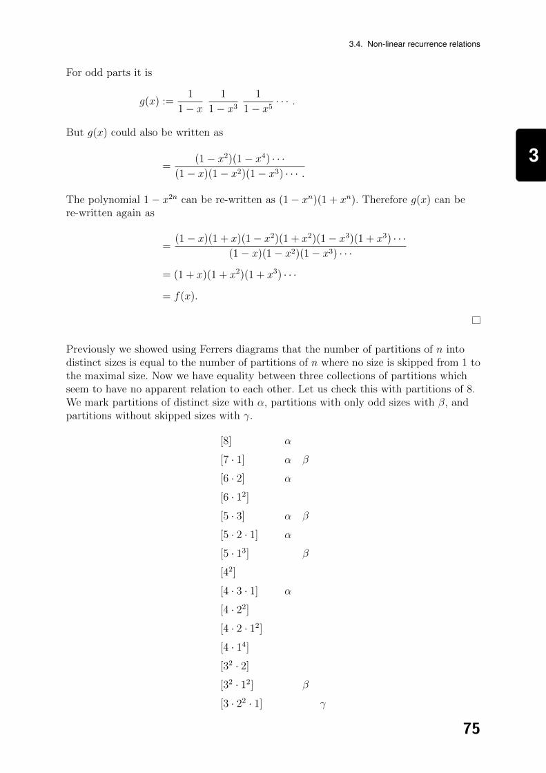
3


For odd parts it is

g(x) :=1

1− x1

1− x31

1− x5 · · · .

But g(x) could also be written as

=(1− x2)(1− x4) · · ·

(1− x)(1− x2)(1− x3) · · · .

The polynomial 1− x2n can be re-written as (1− xn)(1 + xn). Therefore g(x) can bere-written again as

=(1− x)(1 + x)(1− x2)(1 + x2)(1− x3)(1 + x3) · · ·

(1− x)(1− x2)(1− x3) · · ·= (1 + x)(1 + x2)(1 + x3) · · ·

= f(x).

Previously we showed using Ferrers diagrams that the number of partitions of n intodistinct sizes is equal to the number of partitions of n where no size is skipped from 1 tothe maximal size. Now we have equality between three collections of partitions whichseem to have no apparent relation to each other. Let us check this with partitions of 8.We mark partitions of distinct size with α, partitions with only odd sizes with β, andpartitions without skipped sizes with γ.

[8] α

[7 · 1] α β

[6 · 2] α

[6 · 12]

[5 · 3] α β

[5 · 2 · 1] α

[5 · 13] β

[42]

[4 · 3 · 1] α

[4 · 22]

[4 · 2 · 12]

[4 · 14]

[32 · 2]

[32 · 12] β

[3 · 22 · 1] γ

75

3


[3 · 2 · 13] γ

[3 · 15] β

[24]

[23 · 12] γ

[22 · 14] γ

[2 · 16] γ

[18] β γ


Exercise 3.10

Write down the generating functions for the number of partitions of an integer n suchthat

(a) all parts are odd

(b) all parts are of unequal size

(c) the largest part is of size m

(d) one and only one part is of size one

(e) the size of every part is not a power of 2.

Exercise 3.11

Explain why both the sequences ai = i! and bi =1

i!do not have rational generating

functions while the sequence ci =

(i

m

)does have a rational generating function for any

fixed m.

Exercise 3.12

Define a sequence of numbers a0, a1, . . . by a0 = 0, a1 = 1, and for n ≥ 2

an = (a1an−1 + a2an−2 + · · ·+ an−1a1) + 1.

Write down the values of ak for k = 1, 2, 3, 4, 5, 6. What is its generating function? Takethe first and second derivatives of the generating function and show that theirevaluations at zero correspond to the values for a1 and a2. Hint: Similar to the solutionto the Catalan numbers, we see that

ak = 1 + aka0 + ak−1a1 + ak−2a2 + · · ·+ a1ak−1 + a0ak

for k = 2, 3, . . . . Recall that1

1− x is the generating function for the sequence ai = 1 for

all i = 0, 1, . . . .

76

3

3.4. Learning outcomes

Learning outcomes

At the end of this chapter and the relevant reading, you should be able to:

write down the generating function for the number of ways to make change andcalculate these valuesobtain the generating function from a homogeneous linear recurrence relationknow how to multiply, divide and differentiate Laurent seriesbreak down complicated expressions into partial fractionsfind the explicit formula for a generating function, given that the appropriatepolynomial is easy to factoridentify homogeneous linear recurrence relationssolve explicitly for homogeneous linear recurrence relations using tablesperform long division on polynomialsconvert composite linear recurrence relations into a single recurrence relationdetermine the initial conditions that make a sequence go to positive or negativeinfinity.

Solutions to exercises



The answer is2x(2x+ 1)

(1− 2x)3.

Consider first ai = i: The generating function1

(1− y)2corresponds to the polynomial

function ai = i+ 1. Therefore ai = i corresponds to the generating function

1

(1− y)2− 1

1− y =y

(1− y)2.

Then solve for ai = i2. The generating function1

(1− y)3corresponds to the polynomial

function ai =(i+ 2)(i+ 1)

2. Multiply by 2 for 2

1

(1− y)3corresponding to i2 + 3i+ 2.

With the above results for i and 1 we get i2 corresponding to

2

(1− y)3− 3

(1− y)2+

1

1− y .

Put everything on top of1

(1− y)3for

y(1 + y)

(1− y)3. Now substitute y = 2x.

There is another way: take the derivative ofy

(1− y)2= y + 2y2 + 3y3 on both sides and

then multiply the result by y. Lastly substitute y = 2x.

77

3



a1 is equal to 1 and a2 = 2 (in two strides or in one double stride). For n ≥ 3 either theprofessor reaches the n− 1th stair or he does not. In the former case he takes the laststair in a single stride and in the latter case he takes the last two stairs in a doublestride. Therefore an = an−1 + an−2 for n ≥ 3 and with a0 = 1 we have the Fibonnacisequence.


First factor the polynomial 1 + x+ x2 (or finds its roots). Then complete the square:

1 + x+x2

4=−3x2

4⇒

(1 +

x

2

)2=−3x2

4

⇒ 1 +x

2=

√3 i

2x or −

√3 i

2x

1 + x+ x2 =

(1 +

1 +√

3 i

2x

)(1 +

1−√

3 i

2x

).

Notice that (1+√3 i

2)(1−

√3 i

2) = 1−3i2

4= 1. These two complex number are the roots of

unity corresponding to 120 and 240 degrees around the circle (as 1 + x+ x2 is a factorof 1− x3).We can write

a

1 + 1+√3 i

2x

+b

1 + 1−√3 i

2x

=1

1 + x+ x2.

Thus

a+1−√

3 i

2ax+ b+

1 +√

3 i

2bx = 1.

Collecting the coefficients for the powers of x we have a linear system with two variablesand two equations. It solves to a = 3−

√3 i

6and b = 3+

√3 i

6for the explicit formula

an =3−√

3 i

6

(1 +√

3 i

2

)n

(−1)n +3 +√

3 i

6

(√3 i− 1

2

)n

.

We can check by following the rule an = −an−1 − an−2 or doing long division on1

1 + x+ x2. Notice that there are only finitely many numbers for an. Because the roots

of 1 + x+ · · ·+ xk are distinct roots of unity, this will hold for all rules of the forman = −an−1 − · · · − an−k for all n ≥ k.


The number of ways to distribute k pence in coins of value v to n people has thegenerating function

1

(1− xv)n .

But here we have restrictions. The first coin gets distributed to only two people, so with

only the first coin the answer is1

(1− x)2. Adding the second and third coins, and also

78

3


considering that each of these coins can be distributed to only two people, we get

1

(1− x)21

(1− x2)21

(1− x5)2 .



We can start with (1−x)(1−x3) = 1−x−x3 +x4 and divide 1 by 1−x−x3 +x4 or we

can start with1

1− x = 1 + x+ x2 + · · · and then divide by 1− x3. Let us do the latter.

The first number to be placed on top is 1. After subtracting 1− x3 we are left with theremainder x+ x2 + 2x3 + x4 + · · · .The next step gives 1 + x on the top with the remainder x2 + 2x3 + 2x4 + x5 + · · · .Next comes 1 + x+ x2 on top with the remainder 2x3 + 2x4 + 2x5 + x6 + · · · .Not surprisingly, we get the first coefficient other than 1 at the third power, exactly thelevel where there is more than one way to give change. 1 + x+ x2 + 2x3 is on the topwith the remainder 2x4 + 2x5 + 3x6 + x7 + · · · .Next comes

1 + x+ x2 + 2x3 + 2x4

on the top with the remainder 2x5 + 3x6 + 3x7 + x8 + · · · .With 5 less than twice 3 we continue with the coefficient 2 for

1 + x+ x2 + 2x3 + 2x4 + 2x5

on the top and the remainder 3x6 + 3x7 + 3x8 + x9 + · · · .Not surprisingly, with 6 we get more possibilities for giving change than just two. Onthe top is

1 + x+ x2 + 2x3 + 2x4 + 2x5 + 3x6

with the remainder 3x7 + 3x8 + 4x9 + x10 + · · · .The next step gives

1 + x+ x2 + 2x3 + 2x4 + 2x5 + 3x6 + 3x7

on the top and the remainder 3x8 + 4x9 + 4x10 + x11 + · · · .With 8 less than three times 3, the next step gives

1 + x+ x2 + 2x3 + 2x4 + 2x5 + 3x6 + 3x7 + 3x8

on top and the remainder 4x9 + 4x10 + 4x11 + x12 + · · · .The ninth step has

1 + x+ x2 + 2x3 + 2x4 + 2x5 + 3x6 + 3x7 + 3x8 + 4x9

79

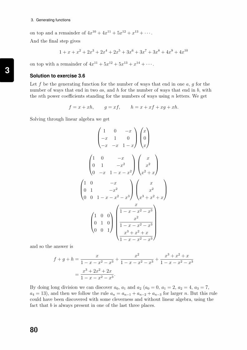
3


on top and a remainder of 4x10 + 4x11 + 5x12 + x13 + · · · .And the final step gives

1 + x+ x2 + 2x3 + 2x4 + 2x5 + 3x6 + 3x7 + 3x8 + 4x9 + 4x10

on top with a remainder of 4x11 + 5x12 + 5x13 + x14 + · · · .


Let f be the generating function for the number of ways that end in one a, g for thenumber of ways that end in two as, and h for the number of ways that end in b, withthe nth power coefficients standing for the numbers of ways using n letters. We get

f = x+ xh, g = xf, h = x+ xf + xg + xh.

Solving through linear algebra we get

1 0 −x−x 1 0

−x −x 1− x

x

0

x

1 0 −x0 1 −x20 −x 1− x− x2

x

x2

x2 + x

1 0 −x0 1 −x20 0 1− x− x2 − x3

x

x2

x3 + x2 + x

1 0 0

0 1 0

0 0 1

x

1− x− x2 − x3x2

1− x− x2 − x3x3 + x2 + x

1− x− x2 − x3

and so the answer is

f + g + h =x

1− x− x2 − x3 +x2

1− x− x2 − x3 +x3 + x2 + x

1− x− x2 − x3

=x3 + 2x2 + 2x

1− x− x2 − x3 .

By doing long division we can discover a0, a1 and a2 (a0 = 0, a1 = 2, a2 = 4, a3 = 7,a4 = 13), and then we follow the rule an = an−1 + an−2 + an−3 for larger n. But this rulecould have been discovered with some cleverness and without linear algebra, using thefact that b is always present in one of the last three places.

80

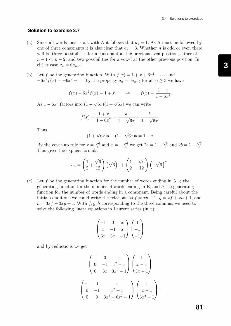
3



(a) Since all words must start with A it follows that a1 = 1. As A must be followed byone of three consonants it is also clear that a2 = 3. Whether n is odd or even therewill be three possibilities for a consonant at the previous even position, either atn− 1 or n− 2, and two possibilities for a vowel at the other previous position. Ineither case an = 6an−2.

(b) Let f be the generating function. With f(x) = 1 + x+ 6x2 + · · · and−6x2f(x) = −6x2 − · · · by the property an = 6an−2 for all n ≥ 3 we have

f(x)− 6x2f(x) = 1 + x ⇒ f(x) =1 + x

1− 6x2.

As 1− 6x2 factors into (1−√

6x)(1 +√

6x) we can write

f(x) =1 + x

1− 6x2=

a

1−√

6x+

b

1 +√

6x.

Thus

(1 +√

6x)a+ (1−√

6x)b = 1 + x

By the cover-up rule for x =√66

and x = −√66

we get 2a = 1 +√66

and 2b = 1−√66

.This gives the explicit formula

an =

(1

2+

√6

12

)(√6)n

+

(1

2−√

6

12

)(−√

6)n.

(c) Let f be the generating function for the number of words ending in A, g thegenerating function for the number of words ending in E, and h the generatingfunction for the number of words ending in a consonant. Being careful about theinitial conditions we could write the relations as f = xh− 1, g = xf + xh+ 1, andh = 3xf + 3xg + 1. With f, g, h corresponding to the three columns, we need tosolve the following linear equations in Laurent series (in x):

−1 0 x

x −1 x

3x 3x −1

1

−1

−1

and by reductions we get

−1 0 x

0 −1 x2 + x

0 3x 3x2 − 1

1

x− 1

3x− 1

−1 0 x

0 −1 x2 + x

0 0 3x3 + 6x2 − 1

1

x− 1

3x2 − 1

.

81

3


With 1− 6x2 − 3x3 in the denominator of all the generating functions this isenough to see the basic relation an = 6an−2 + 3an−3 for sufficiently large n and, ofcourse, the initial values are easy to calculate. One could also continue the processof solving the linear equations to get

h =1− 3x2

1− 6x2 − 3x3, g =

1− 5x2

1− 6x2 − 3x3, f =

−1 + x+ 6x2

1− 6x2 − 3x3

and the complete generating function:

1 + x− 2x2

1− 6x2 − 3x3.

The linear recurrence relation is a0 = 0, a1 = 1, a2 = 4, a3 = 9, and for n ≥ 4an = 6an−2 + 3an−3 (which can be discovered by knowing only the denominator1− 6x2− 3x3 and a little logic to calculate an up to n = 3). Also, as in the previousexercise, the relation an = 6an−1 + 3an−2 can be discovered with some clevernessand without linear algebra from the fact that there is alternation between vowelcombinations and consonants.

Solution to exercise 3.8x(x+ 1)

(1− x)3is the generating function for an = n2, which we have discovered already.

Let f(x) = 1 + a1x+ · · · be the generating function in question. We can write

f(x) = 1 + a1x + a2x2 + · · ·

−3xf(x) = − 3x − 3a1x2 − · · ·

+2x2f(x) = + 2x2 + · · ·

+x(1 + x)

(1− x)3= + x + 4x2 + · · ·

We therefore get

(1− 3x+ 2x2)f(x) +x(1 + x)

(1− x)3= 1 + a1x− 2x.

Factor 1− 3x+ 2x2 = (1− 2x)(1− x) and put together for

f(x) =1− 6x+ a1x+ 8x2 − 3a1x

2 − 7x3 + 3a1x3 + 2x4 − a1x4

(1− 2x)(1− x)4

=b

1− 2x+

c

1− x +d

(1− x)2+

e

(1− x)3+

g

(1− x)4

and

1− 6x+ a1x+ 8x2 − 3a1x2 − 7x3 + 3a1x

3 + 2x4 − a1x4

= (1− x)4b+ (1− x)3(1− 2x)c+ (1− x)2(1− 2x)d+ (1− 2x)(1− x)e+ (1− 2x)g.

82

3


Now solve for b = 0 with the cover up rule using x = 12

for the answer a1 = 12 (obtainedby multiplying everything by 16 and simplifying). In the event that b = 0 and a1 = 12,it is the value of g that matters. Plug in x = 1 and a1 = 12 for g = 2. Hence if a1 is 12or more then the sequence goes to positive infinity and if a1 is less than 12 then tonegative infinity.


Consider first the generating function f = a0 + a1x+ · · · where ak is the number ofregions of R generated by k points. Given the intersection properties, it follows thatak = k + 1, which is true even for the case of k = 0. This yields

f =1

(1− x)2.

Next consider the generating function g = b0 + b1x+ · · · where bk is the number ofregions of R2 generated by k lines (assuming by induction that these numbers areindependent of the lines chosen, so long as the intersection properties hold). Considerthe regions B1, . . . , Bbk−1

of R2 generated by k − 1 lines. The kth line will cut throughsome of these regions and not cut through others. The number of regions created by klines will be bk−1 plus the number of the Bi cut into two by the new kth line. Look atthe intersections of the B1, . . . , Bbk−1

with the kth line. They are regions of the kth linecreated by k − 1 points on this line (intersections of the k − 1 first lines with the kthline). This is the number ak−1 = k. We conclude that b0 = 1 and bk = bk−1 + ak−1 for allk ≥ 1, or g = xg + xf + 1. This solves to

(1− x)g = 1 +x

(1− x)2=

1− x+ x2

(1− x)2⇒ g =

1− x+ x2

(1− x)3.

Lastly consider the generating function h = c0 + c1x+ · · · where ck is the number ofregions of R3 generated by k planes (again well defined by an induction assumption).Consider the regions C1, . . . , Cck−1

generated by k − 1 planes. We perform the sameargument, that the number of regions with k planes is the sum of the number ck−1 withk − 1 planes plus the number of the regions C1, . . . , Cck−1

cut into two by the kth plane,and then relate this to the answer for the lower dimensions. We get c0 = 1 andck = ck−1 + bk−1 for all k ≥ 1, or h = xh+ xg + 1. This solves to

(1− x)h = x1− x+ x2

(1− x)3+ 1 =

1− 2x+ 2x2

(1− x)3⇒ h =

1− 2x+ 2x2

(1− x)4.

Solving with partial fractions yields

a

1− x +b

(1− x)2+

c

(1− x)3+

d

(1− x)4=

1− 2x+ 2x2

(1− x)4

or

a(1− x)3 + b(1− x)2 + c(1− x) + d = 1− 2x+ 2x2.

83

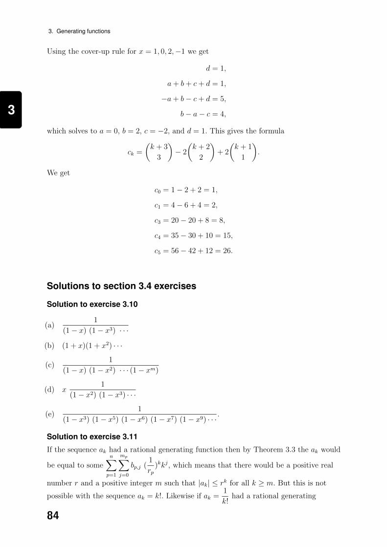
3


Using the cover-up rule for x = 1, 0, 2,−1 we get

d = 1,

a+ b+ c+ d = 1,

−a+ b− c+ d = 5,

b− a− c = 4,

which solves to a = 0, b = 2, c = −2, and d = 1. This gives the formula

ck =

(k + 3

3

)− 2

(k + 2

2

)+ 2

(k + 1

1

).

We get

c0 = 1− 2 + 2 = 1,

c1 = 4− 6 + 4 = 2,

c3 = 20− 20 + 8 = 8,

c4 = 35− 30 + 10 = 15,

c5 = 56− 42 + 12 = 26.



(a)1

(1− x) (1− x3) · · ·

(b) (1 + x)(1 + x2) · · ·

(c)1

(1− x) (1− x2) · · · (1− xm)

(d) x1

(1− x2) (1− x3) · · ·

(e)1

(1− x3) (1− x5) (1− x6) (1− x7) (1− x9) · · · .


If the sequence ak had a rational generating function then by Theorem 3.3 the ak would

be equal to somen∑

p=1

mp∑

j=0

bp,j (1

rp)kkj, which means that there would be a positive real

number r and a positive integer m such that |ak| ≤ rk for all k ≥ m. But this is not

possible with the sequence ak = k!. Likewise if ak =1

k!had a rational generating

84

3


function then also by Theorem 3.3 there would be a positive real number r and apositive integer m such that |ak| ≥ rk for all k ≥ m, something also impossible.

However, for a fixed m the expression

(i

m

)as a function of i is a polynomial in i,

hence by Theorem 3.3 it has a rational generating function.


The first values are a0 = 0, a1 = 1, a2 = 2, a3 = 5, a4 = 15, a5 = 51, and a6 = 188. Let fbe the generating function. According to the recurrence relation, for every n ≥ 2 the

nth coefficient of f 2 plus one is equal to the nth coefficient of f . Recalling that1

xis

equal to 1 + x+ x2 + · · · , this allows us to write f 2 − f +1

xequal to a polynomial of

degree no more than 1. Since f starts out with 0 + x we know that f 2 − f +1

xmust be

equal to −x+ 1 + x = 1. Completing the square gives f 2 − f +1

4=

5

4− 1

1− x . This

solves to f(x) =1

2+

√5

4− 1

1− x or f(x) =1

2−√

5

4− 1

1− x . Since we are given that

f(0) must be equal to 0:

f(x) =1

2−√

5

4− 1

1− xmust be the generating function. The first derivative is

1

2(1− x)2

(5

4− 1

1− x

)− 12

and the second derivative is

1

(1− x)3

(5

4− 1

1− x

)− 12

+1

4(1− x)2

(5

4− 1

1− x

)− 32

.

The first derivative evaluated at 0 is 1 and the second derivative evaluated at 0 is 4.The first must be divided by 1! = 1 to get a1 = 1 and the second must be divided by 2!to get a2 = 2.

85

3


86

discrete mathematics and algebra - university of london

Documents