discrete element method modeling for the failure analysis
TRANSCRIPT

Article
Discrete element method modeling for the failure analysis ofdry mono-size coke aggregates
Alireza Sadeghi-Chahardeh 1 , Roozbeh Mollaabbasi 1 , Donald Picard 2 , Seyed Mohammad Taghavi 3 and
Houshang Alamdari 1,*
�����������������
Citation: Sadeghi-Chahardeh, A.;
Mollaabbasi, R.; Picard, D.; Tessier, J.;
Taghavi, S.M.; Alamdari, H.; Discrete
element method modeling for the
failure analysis of dry mono-size coke
aggregates. Preprints 2021, 1, 0.
https://doi.org/
Received:
Accepted:
Published:
Publisher’s Note: MDPI stays neutral
with regard to jurisdictional claims in
published maps and institutional affil-
iations.
1 Aluminum Research Centre–REGAL, Mining, Material, and Metallurgy Engineering Department, UniversitéLaval, 1065 Avenue de la Médecine, Québec, QC G1V 0A6, CANADA; [email protected](A.S.C.), [email protected] (R.M.), [email protected] (H.A.)
2 Aluminum Research Centre–REGAL, Civil Engineering Department, Université Laval , Québec, QC G1V 0A6,CANADA; [email protected] (D.P.)
3 Chemical Engineering Department, Université Laval, 1065 Avenue de la Médecine, Québec, QC G1V 0A6,CANADA; [email protected] (S.M.T.)
* Correspondence: [email protected]
Abstract: An in-depth study of the failure of granular materials, which is known as a mechanism togenerate defects, can reveal the facts about the origin of the imperfections such as cracks in the carbonanodes. The initiation and propagation of the cracks in the carbon anode, especially the horizontalcracks below the stub-holes, reduce the anode efficiency during the electrolysis process. In orderto avoid the formation of cracks in the carbon anodes, the failure analysis of coke aggregates canbe employed to determine the appropriate recipe and operating conditions. In this paper, it will beshown that a particular failure mode can be responsible for the crack generation in the carbon anodes.The second-order work criterion is employed to analyze the failure of the coke aggregate specimensand the relationships between the second-order work, the kinetic energy, and the instability of thegranular material are investigated. In addition, the coke aggregates are modeled by exploiting thediscrete element method (DEM) to reveal the micro-mechanical behavior of the dry coke aggregatesduring the compaction process. The optimal number of particles required for the failure analysisin the DEM simulations is determined. The effects of the confining pressure and the strain rate astwo important compaction process parameters on the failure are studied. The results reveal thatincreasing the confining pressure enhances the probability of the diffusing mode of the failure in thespecimen. On the other hand, the increase of strain rate augments the chance of the strain localizationmode of the failure in the specimen.
Keywords: Carbon anode production, Crack generation, Discrete element method, Failure analysis,Second-order work criterion, Strain localization
1. Introduction
Carbon anodes are part of the chemical reaction of the alumina reduction and areconsumed during the Hall-Héroult electrolysis process. The mechanical and chemical qual-ities of the carbon anodes directly affect the technological, economical, and environmentalaspects of the aluminum production process. The carbon anode production accounts for 17% of the total cost of the aluminum smelting [1]. To produce one ton of aluminum, theoret-ically, 334 kg of carbon would be required. However, in practice, the required carbon ishigher and roughly about 415 kg per ton of aluminum [2]. The carbon anodes are composedof three major parts, i.e. the calcined petroleum coke (65 wt. %), the recycled anode (butt,20 wt. %), and the coal tar pitch (15 wt. %). Initially, the coke particles are crushed andsieved to the required size distribution, and they are mixed with the granulated recycledbutts. The dry aggregates are then heated to about 160 ◦C and mixed with the coal tar pitchat 150–180 ◦C. The coal tar pitch binds the coke and butt particles. The obtained mixture iscalled the anode paste. The anode paste goes through the vibro-compaction or the pressingprocess to form the green anode blocks. To improve the mechanical strength and electricalconductivity, the green anodes are baked at a temperature of 1100 ◦C. Then, the obtainedbaked anodes can be used as electrodes in the aluminum smelters [3].
Preprints (www.preprints.org) | NOT PEER-REVIEWED | Posted: 15 March 2021 doi:10.20944/preprints202103.0393.v1
© 2021 by the author(s). Distributed under a Creative Commons CC BY license.

2 of 30
Figure 1. Images of cuts made on baked carbon anodes which are manufactured at the Alcoa Deschambault Québec (ADQ)smelter [4]. (The size of cracks in these images has been virtually enlarge for a clearer visual appreciation).
High mechanical strength and electrical conductivity, homogeneity, as well as lowreactivity towards carbon dioxide and air, are the important quality indices of the carbonanodes [5]. The main parameters determining the final anode quality are categorizedinto two essential groups; the material properties and the process parameters [6]. Thevariations in the properties of the raw materials are considered as one of the most significantchallenges in the anode manufacturing industry. This quality variation is due to the factthat the raw materials come from different sources. When the material properties arechanged, the paste formation and the process parameters including the mixing variablesand the compaction parameters should be re-adjusted in such a way to compensate for theeffects of the variations and to keep the anode quality consistent. Moreover, the sufficientmixing power and time, the optimized speed of the vibro-compaction, and the confiningpressures, as well as the proper temperature, are the most important process parametersdetermining the mixing effectiveness and the anode quality. An efficient mixing results ina homogeneous distribution of the coke and the coal tar pitch, and lower porosity in thepaste that improves the anode characteristics such as the density and the thermal shockresistance [5]. In addition, any changes in either the speed and load of pressing forming orthe frequency and dead-weight of the vibro-compaction process influence the homogeneityof the density of the green anodes, as well as the quality of the baked anodes [7]. Similarly,the higher baking temperature leads to larger crystallite sizes and a more homogeneousstructure of the pitch-coke, which reduces the electrical resistivity and the consumptionrate of the carbon anodes [8].
Any defects such as the internal and the external cracks and the density distributionaffect the carbon anode consumption rate and remarkably increase the process costs [7].The presence of the cracks reduces the mechanical strength and the electrical conductivityof the baked carbon anode, thereby reducing the life of the carbon anode, disrupting thecell stability, and increasing the greenhouse gas emissions [6]. Given that all the steps ofanode production are done at high temperatures and the components of the anode pasteare opaque, it is not easy to investigate the origins of the cracks. The cracks can be formedduring the green carbon anode preparation, as well as during the baking process [9,10].Many researchers have attempted to discover the reasons for the formation of the cracks inthe carbon anodes. Menard [11] attributed the generation of the cracks during the green
Preprints (www.preprints.org) | NOT PEER-REVIEWED | Posted: 15 March 2021 doi:10.20944/preprints202103.0393.v1

3 of 30
anode formation to two factors, trapping compressed air in the anode paste during theformation and inhomogeneous distribution of the binder, which causes adhesion betweenthe coke particles. Moreover, Amrani et al. [12] ascribed the crack formation to the releasingof the volatiles from the coal-tar pitch during the baking process, which can create pressureinside the carbon anodes.
Three major types of the cracks can develop in the carbon anodes: corner, vertical,and horizontal cracks [13]. The corner cracks predominantly appear after the anode isset into the electrolysis cell due to the thermal shock [14]. The vertical cracks are createdmainly during the baking process. The high temperature gradient inside the carbon anodedue to the high heating rate provides the tensile stresses required to create the verticalcracks [8]. The horizontal cracks of the anodes are the most detrimental to the electrolysisoperation [13]. Under normal circumstances, the stresses caused by the thermal shockcannot generate these types of cracks [13]. These defects should already appear as smallhorizontal cracks that are likely to occur during the formation process [13]. Boubaker etal. [4] reported a kind of the horizontal cracks below the stub-holes of the baked carbonanodes. In Figure 1, the baked carbon anodes are cut from the middle and shows thehorizontal cracks under the stub-holes. Although these cracks are not present in all theanodes, they are accidentally observed beneath the stub-holes. In the compaction process,however, the compression stresses around the stub-holes appear to be higher than in otherparts of the carbon anode. Hence, It seems strange to have these types of cracks wherethey are probably denser than elsewhere in the anode [15]. On the other hand, becausethese cracks are the opening type, the tensile stresses perpendicular to the direction of thecrack growth is required to generate them [16]. However, the origin of these tensile stressesbeneath the stub-hole is not known [4].
Many investigations have been conducted to find the cause of the formation of thecracks [15,17]. Due to the high temperature of the forming process and the opacity of thecarbon anode paste, the experimental investigations are not easily performed. Chaoukiet al. [15] proposed a constitutive law to simulate the anode paste during the compactionprocess. Although this model can reveal the density gradient due to the stub-hole, it is notcapable of demonstrating the formation of the horizontal cracks below the stub-hole [15,17].This limitation stems from the fact that the granularity nature of the anode paste cannot betaken into account by phenomenological models such as finite element methods [18]. Onthe other hand, several attempts have been made to investigate the behavior of anode pasteusing the discrete element method (DEM), which considers grains as the basic elementfrom which the mechanical behavior of granular materials originates [6,19]. Despite the factthat modeling anode paste with all its complexities, including different size distribution,particle shape, solid-fluid interaction, and coal-tar pitch dependence on temperature, is achallenging task, DEM has shown that it is able to simulate successfully some properties ofthe anode coke aggregates such as the bulk density [20] and the electrical resistivity [21].However, investigating the causes of the horizontal cracks under stub-holes requires morein-depth analysis. Hence, a comprehensive study of the distinct behaviors of granularmaterials subjected to compression loading conditions can shed light on the hidden truthof this problem.
The granular materials are generally defined as those composed of the smaller par-ticles, and in our case, those whose mechanical behavior is governed by the interactionbetween the particles [18]. When the granular material is exposed to a compression load, itreaches a stress state wherein it is no longer able to sustain any deviatoric load increment.At such a limited stress state, if an additional load is imposed the state of the materialchanges suddenly with the occurrence of large deformations, cracks, fragmentation, etc[22]. This circumstance, which is associated with a sudden decrease in the number ofgrain contacts, is called failure [23]. The sudden reduction in the grain contacts leads to asignificant increase in the number of degrees of freedom which implies the possibility ofrapid relative displacements between the grains. Due to these rapid relative displacementsbetween the grains, the failure is a physical phenomenon that can be regarded as a state
Preprints (www.preprints.org) | NOT PEER-REVIEWED | Posted: 15 March 2021 doi:10.20944/preprints202103.0393.v1

4 of 30
from which a transition from a quasi-static regime to a dynamical regime is possible undercertain constant loading parameters [24]. For the materials with an associative flow rule,as it is generally assumed for metals, the symmetry of the elasto-plastic tensor leads tothe compelling fact that the failure occurs in the plastic limit condition. However, forgranular materials, which are known to have non-associated flow rules and consequentlynon-symmetry in the elasto-plastic tensor, the failure can be met before the plastic limitcondition (Mohr-Coulomb criterion) [25]. The mathematical interpretation of the failureis usually attributed to the existence of a limit load that cannot be exceeded for a givenmechanical system under some boundary and initial conditions [26].
The failure in the granular materials is initiated by the instability of these materials[27]. The instability can be either geometric such as structural instability [28], or materialsuch as constitutive behavior and force chains buckling [25,29]. The geometric instability isassociated with the tendency of the configuration to pass from one deformation pattern toanother [28]. For instance, the critical condition of a long, slender column that is axiallyloaded is a state of transition from pure compression to a combination of compression andbending. Therefore, this type of instability is a function of the geometry of the specimenand its loading [30]. On the other hand, material instability is defined as a property of thematerial that converts an initially homogeneous deformation field into a heterogeneousdeformation field [31]. The material instability is related to the size of the materiallyintrinsic length scales, which is called microstructure, and the magnitudes of the lengthscale of the initial perturbations [29,31]. For example, local buckling of particle force chainsis considered as a material instability [29,32].
The material instability leads to the loss of uniqueness of the solution of the underlyinggoverning equations, hence to a bifurcation problem [33]. When a mechanical state belongswithin the bifurcation domain, failure is possible depending on the loading parameters,loading history, disturbances, and imperfections in the system [22]. Due to this dependenceon small perturbations, the failure can also be viewed as an instability phenomenon in thebasic Lyapunov sense [34]. Lyapunov’s definition of stability expresses that for a givenrate-independent material, a stress-strain state for a given strain history is called stableif any small change of any admissible loading leads to a small change of the response.However, the main question that comes to mind is, according to Lyapunov’s definition ofstability, how can be shown a stress-strain state is unstable strictly inside the plastic limitsurface?
Two concepts of failure are built around the above-mentioned question of describingthe failure. The first one is the notion of controllability [35] and the second one is thesustainability of equilibrium states [36]. Nova [35] proceeded by defining controllabilityas the ability of a material (or a model) to provide one and only one (existence anduniqueness) response to any loading path for which some strain components and theother stress components are prescribed. According to [35], granular materials lose theircontrollability at a certain stress level and after that point, the specimen does not give rise toa unique material response under any arbitrary incremental loading program. At this point,the stiffness tensor is no longer positive definite. It has been shown that as soon as thestiffness tensor becomes positive semi-definite, there is a particular program that leads toinfinite solutions and unconditional controllability is lost [37]. The concept of controllabilityis an interpretation of the Lyapunov definition of stability. As the notion of controllabilityapplies to a given loading program, therefore, this is not an intrinsic characteristic ofthe mechanical state of the system [35]. On the other hand, another interpretation of theLyapunov definition of stability is about the sustainability of the mechanical state of thesystem. The sustainability of equilibrium states defined as an ability of a mechanical systemloaded with specific control parameters to evolve toward another mechanical state froma given equilibrium state, with no change in the control parameters [36]. If this is true,the equilibrium state of the material is reputed unsustainable, and the subsequent lossof sustainability corresponds to a proper bifurcation mode. From a mechanical point of
Preprints (www.preprints.org) | NOT PEER-REVIEWED | Posted: 15 March 2021 doi:10.20944/preprints202103.0393.v1

5 of 30
view, it means that a system that is initially in equilibrium can generate kinetic energyspontaneously and without any external disturbances [26,36].
Due to the difficulty with Lyapunov definition of stability, there was a need for arelated manageable criterion of failure for the practical use in the investigation of thegranular materials [38,39]. To compensate for this issue, Hill’s second-order work criterionof stability has been introduced. According to Hill [40], a stress-strain state is unstable ifthere exists one loading direction which can be pursued in an infinitesimal manner withoutany input of the energy from an external source. Although Hill’s criterion and Lyapunov’sdefinition of stability are not related in a general manner [41], the concepts of controllabilityand sustainability are equivalent to the Hill’s criterion in the classical elasto-plasticity [35]and the failure of granular materials [39,42]. Therefore, in spite of the fact that this criteriondoes not specify the mode of material failure [24], it can predict the necessary conditionsfor the occurrence of a failure in the granular materials.
Various modes of failure in granular materials have been observed in practice. Thanksto experimental observations, there are two broad classes of failure modes that arise in thegranular materials due to some instabilities [43]. In the granular materials, excluding flutterinstabilities, two material failure modes are of interest: localized and diffuse failure modes.At a material point scale, the localized failure mode corresponds to a transition from ahomogeneous strain pattern to an inhomogeneous one, characterized by the appearance ofa system of bands in which strains concentrate [44]. These narrow zones where deforma-tion is concentrated are called localized bands. Depending on the loading path and theirkinematic attributes, shear, dilation, or compaction bands may be developed [45]. Whilethe shear bands are predominated by shearing, the dilation and compaction bands areformed primarily by volumetric deformation and they are characterized by local volumeexpansion and local volume reduction, respectively [45]. The strain localization of thegranular materials has been studied by many researchers through theoretical [44,46–48], ex-perimental [49–54], and numerical methods [55–58]. There have been attempts to simulatethe phenomenon of the strain localization in the granular material, especially in the sandsamples, based on either continuum mechanics by using the finite element method (FEM)[55,56] or micro-mechanics by using the discrete element methods (DEM) [53,57]. Thefinite element methods (FEM) require the constitutive relation of the material, while thereare no reliable constitutive laws that can accurately predict the behavior of the granularmaterials [59]. It should be noted that the constitutive laws derived from the classicalcontinuum mechanics do not take into account the dimensions of the granular elements[18,60]. Consequently, these constitutive laws suffer from pathological mesh-dependencywhen they are employed in the failure analyses [61,62]. However, the discrete elementmethod can provide applicable equipment for considering the internal length scale of thegranular material without involving the sophisticated mathematics of the non-classicalcontinuum mechanics [63]. In addition, a combination of the latter two methods, calledmulti-scale methods, is also used to model the strain localization in the granular materials,which benefits from both FEM and DEM [18,58,62,64,65].
On the contrary, the diffusing failure mode corresponds to a homogeneous occurrenceof the failure in which no visible pattern of localization exists [66]. A chaotic, unstructuredstrain field dominates [41]. This failure mode can be observed mostly in the loose sandspecimens for classical tests [67]. Diffusing failure does not occur in the dense sand underundrained conditions [68]. This is the case, for instance, for the isochoric triaxial test carriedout on a loose sand specimen. At the deviatoric peak, an infinitesimal loading disturbanceis sufficient to provoke the abrupt collapse of the specimen without any localization pattern[38,66]. While the localized failure is predicted by the vanishing values of the determinantof the acoustic tensor [46], known as classical bifurcation analysis, the second-order workcriterion is mostly used as a proper indicator of the diffuse failure mode [66]. Althoughthere are differences in the kinematics properties of the two failure modes, [69] showedthat both localized and diffuse failure can be predicted through the classical bifurcationanalysis. Despite the difficulty in finding a proper constitutive law that describes the
Preprints (www.preprints.org) | NOT PEER-REVIEWED | Posted: 15 March 2021 doi:10.20944/preprints202103.0393.v1

6 of 30
granular material’s behavior, the bifurcation analysis has been used widely to predictfailure in the sands [56,70], the rocks [71], and the fluid-saturated granular soils [72,73].Moreover, it has been shown that the second-order work criterion is capable to detectboth the diffuse and the localized failure modes [24]. This criterion, unlike the classicalbifurcation analysis, does not require necessarily a constitutive law to predict failure [74].
Comprehension of failure as a mechanism to generate defects in granular materialcan reveal the facts about the origin of the imperfections such as cracks in the granularmaterials (e.g. see [45,75] and the references cited in them). In geology, the localizedbands are recognized as the main mechanism of fault formation in sandstone whichprecedes the formation of the larger faults [76,77]. As these localized bands are usuallyassociated with porosity reduction, they may provide a natural barrier to fluid flows andform hydrocarbon reservoirs and aquifers [78,79]. Another type of localized bands, calledcompaction bands, is formed by the accommodation of pure compaction (with little orno shear) in the tabular zone perpendicular to the maximum compression direction inthe sandstone or the sedimentary rocks [80–82]. There are compelling evidence for theexistence and the formation of compaction bands in the granular materials that are exposedto the compressive stress states both in the laboratory and in the theory [82]. Althoughcompaction bands were first recognized in the sandstone [80], similar phenomena appearto be common in the other porous materials [83]. For instance, Bastawros et al. [84] wereable to illustrate the formation of the compaction bands in a cellular aluminum alloy uponaxial compression through a digital image correlation procedure. Similar observations hadbeen reported for steel foams [85] and polycarbonate honeycombs [86] in which inherentpore collapse has mainly caused the formation of the compaction bands.
The characteristics of the compaction bands, such as being perpendicular to themaximum principal compression direction, as well as the similarity in the way of loading,which is mainly compressive, have led us to the idea that the horizontal cracks beneaththe stub-holes in the carbon anodes can be generated by these bands. Figure 2 shows howinternal tensile stresses could generate inside the carbon anode even in the absence of anexternal load. When the compressive stresses are applied to the carbon anode paste, dueto the stub-hole shape effect, the areas below the stub-holes subject to more compactionthan their neighboring areas (Figure 2 (a)). It is assumed that this additional compressioncan cause the compressive strain to accumulate in a narrow rectangular region, resultingin a compression band (dashed rectangle in Figure 2 (b)). After removing the externalload from the material, due to the viscoelastic properties of the carbon anode paste, thecompression accumulated in the compaction bands causes residual tensile stresses in thestub-hole region, as well as residual compressive stresses in the neighboring areas (Figure2 (c)). Accordingly, the compaction bands could be responsible for the tensile stresseswhich are required for the generation of these type of cracks. This phenomenon is similarto the inclusion problem in the elastic media described by Eshelby [87]. Although manyresearchers used an analogous method to predict the initiating of the compaction bandsin the porous rocks [81,88–90], the factors influencing the various manifestations of thecompression bands are still unknown [82]. Therefore, understanding the failure behaviorof the granular materials is of great importance to find the mysterious phenomena ofcompaction band formation. In addition, due to the fact that detection of the compactionbands is difficult in either the field or the laboratory [82], it is possible that compactionbands are present in virtually all the carbon anodes (even in the cases where there are nohorizontal cracks). Although some parameters, such as thermal shocks or shrinkage of thecoal-tar pitch during the baking process, affect the formation of the cracks in the carbonanodes, the compaction bands are a mechanism that can create a susceptible region underthe stub-holes to generate the horizontal cracks. Therefore, it is necessary to determinethe factors of the physical conditions and the material characteristics associated with theformation of the compaction bands in the case of a systematic investigation.
As aforementioned, the existence of compaction bands in the visco-elastic anodepaste creates a susceptible area for the horizontal crack formation. While the temperature
Preprints (www.preprints.org) | NOT PEER-REVIEWED | Posted: 15 March 2021 doi:10.20944/preprints202103.0393.v1

7 of 30
(a) (b) (c)
Figure 2. Generation of the residual tensile stresses due to compaction band formation. (a) The carbon anode paste beforethe compaction process. (b) The carbon anode paste during the compaction process and the formation of the compactionband (dashed rectangle). (c) Creating residual stresses in the absence of the external pressure. (The red arrows indicate thecompression stresses and the blue ones show the tensile stresses).
and coal-tar pitch content affect the viscous part of the anode paste, the coke particlecharacteristics influence the elastic part of the anode paste behavior [5]. Therefore, it seemsreasonable to consider only the coke particles for the failure analysis. In addition, thecoarse coke particles have been shown to form a skeleton that controls the main mechanicalbehavior of coke aggregates [91]. Hence, for the sake of simplicity, we will consider thecoarse coke particles with spherical shape for our investigations. Accordingly, in this paper,the second-order work criterion for the failure of the granular material will be reviewedand the influence of failure on the kinetic energy of the system will be explained in Section2. In addition, the ability of the second-order work criterion in diagnosing the failure ofthe granular material will be discussed. In Section 3, the concept of the discrete elementmethod will be presented. The criteria for choosing the proper representative volumeelement (RVE) will be studied. In Section 4, the strain localization analysis is presentedbased on the second-order work criterion and the evolution of the mode of the localizedbands will be discussed. The most salient results of this work will be summarized anddiscussed in Section 5.
Throughout this paper, the material time derivatives of any variable ψ will be dis-tinguished by denoting Dψ
Dt and the particulate time derivative of ψ defined as ψ. Thefirst-order tensors (vectors) and the second-order tensors, respectively, denoted by lower-case bold Latin (v) and upper-case bold Latin (F). Moreover, the subscript 3 throughout thepaper indicates the axial direction, while the subscripts 1 and 2 were designated as lateraldirections.
2. Second-order work criterion
In mechanical problems, where the existence of a potential energy function can beassumed, with some particular hypotheses on conservative and dissipative forces, stabilityis ensured if this potential function has a strict minimum. Due to complex dissipativephenomena, a potential energy function does not exist in mechanics problems involvinggranular media [38]. Therefore, the material instabilities thus cannot be studied throughthe analysis of potential energy function. In other words, these instabilities are linked tothe inherent deformation mechanisms of the granular material and do not depend on thepotential energy. In addition, the theoretical investigations, the numerical analyses, andthe experimental results highlight that the concept of failure is related to the developmentof kinetic energy [26,68,92,93]. As a consequence, it is necessary to have criteria that relatethe kinetic energy of granular material to the control parameters (such as strain or stress
Preprints (www.preprints.org) | NOT PEER-REVIEWED | Posted: 15 March 2021 doi:10.20944/preprints202103.0393.v1

8 of 30
Figure 3. Definition of the First Piola-Kirchhoff stress tensor and Cauchy stress tensor and transformation of a material system.
at the boundaries). Hence, the issue of stability will be investigated using Hill’s second-order work criterion [40]. This sufficient condition of failure states that a stress-strainstate is stable if, for all (δP, δF) in the semi-Lagrangian formulation or (δσ, δǫ) in Eulerianformulation (by assuming small deformations and neglecting geometrical aspects) linkedby the constitutive relation, the second-order work is strictly positive [94]:
d2W =∫∫∫
V0
δPij δFij dV0 > 0 (semi-Lagrangian expression) ,
d2W =∫∫∫
V
δσij δǫij dV > 0 (Eulerian expression) ,(1)
where Pij is the first Piola-Kirchhoff stress tensor, Fij the general term of the deformationgradient tensor, σij the Cauchy stress tensor and, and ǫij is the strain tensor. Thus, accordingto Hill, a stress-strain state is unstable if at least one loading direction exists that can bepursued in an infinitesimal manner without any input of energy from the outside. It isworth noting that the vanishing of the second-order work implies the loss of controllabilityof the loading program, independently of the constitutive relations has been proved,independently of the constitutive relations [37]. Although this sufficient condition isnot based on thermodynamic principles, it still remains a valuable tool for investigatingpotential instabilities [38]. The nullity of the second-order work criterion is a powerful toolto describe any kind of quasi-static material instability by taking into account that flutterinstabilities are dynamic.
2.1. kinetic energy of the granular system and external and internal second-order work
An attempt for the definition of the failure in the granular material was made in theprevious section, and this related to a transition (bifurcation) from a quasi-static regimetoward a dynamic one. In this section, the mathematical description of the second-orderwork criterion is developed and the conditions in which the kinetic energy of the granularmaterial system may increase will be investigated. For this purpose, a system consisting ofgranular material, with a volume, V0, and a surface boundary, S0, initially in a configuration,C0, is considered. With a loading history, the system is in a current configuration, C, witha volume, V, and the surface boundary, S, in equilibrium under a prescribed externalload. Each material point in the volume V0 is transformed into a material point in thevolume V (Figure 3). All the material points in the volume V0 are displaced along with thedeformation of their geometric properties, including the surface vector, the area, and thevolume. During this transformation, the material is subjected to a rigid body motion, along
Preprints (www.preprints.org) | NOT PEER-REVIEWED | Posted: 15 March 2021 doi:10.20944/preprints202103.0393.v1

9 of 30
with the pure strain induced by the stretching and the spinning deformations. If largeamounts of strain take place, the initial configuration, C0, will be significantly differentfrom the current configuration, C.
As the Cauchy stress tensor is not objective (in the rigid body transformation, itgives different values), the first Piola-Kirchhoff stress tensor and the conservation of themechanical energy in the material description are used [95,96]. It should be noted that thefirst Piola-Kirchhoff stress vector is the vector t0(X, t, n0), which is parallel to the Cauchystress t(x, t, n), but measures the force per unit undeformed area (see Figure 3). The balanceof the kinetic energy of a system with neglecting the body force in the material description(configuration C0) can be derived as [97]:
D
DtK(t) = Pext(t)−Pint(t) , (2)
orD
Dt
∫∫∫
V0
(12
ρ0v · v
)
dV0 =∫∫
S0
Pn0 · vdS0 −∫∫∫
V0
P : FdV0 . (3)
Equation (3), expresses that the rate of change of the kinetic energy, K(t), is equal to thedifference between the power of the external forces, Pext(t), and the power of the stresses,Pint(t). The stress power, P : F, given in term of the first Piola-Kirchhoff stress tensorP = JσF−T and the deformation gradient F. Note that the stress power P : F refers to theunit undeformed volume. By taking the time derivative of Equation (3) yields:
D2
Dt2
∫∫∫
V0
(12
ρ0v · v
)
dV0 =∫∫
S0
(Pn0 · v + Pn0 · v
)dS0 −
∫∫∫
V0
(P : F + P : F
)dV0 . (4)
Furthermore, the two-order Taylor expansion of the kinetic energy reads:
K(t0 + ∆t) = K(t0) + ∆tK(t0) +(∆t)2
2K(t0) + H.O.T. (∆t) . (5)
Since the velocity of the system in the initial time is equal to zero (quasi-static), the amountof the kinetic energy K(t0) and its first time derivative K(t0) must be equal to zero [93]. Inaddition, if ∆t is considered to be small, then the higher-order terms of ∆t (H.O.T. (∆t)) canbe ignored. Therefore, by substituting in Equation (5), the kinetic energy in a very smalltime interval could be predicted as:
K(t0 + ∆t) =(∆t)2
2K(t0) . (6)
Therefore, by combining Equation (4) and (6), an approximation of the kinetic energychanges in a quasi-static system will be obtained as a function of the external and theinternal stress powers.
K(t0 + ∆t) =(∆t)2
2
Pext(t)︷ ︸︸ ︷∫∫
S0
(Pn0 · v + Pn0 · v
)dS0 −
Pint(t)︷ ︸︸ ︷∫∫∫
V0
(P : F + P : F
)dV0
. (7)
Based on Equation (7), the evolution of the kinetic energy of a granular system for everytime step can be expressed as the difference between the rate of the external and the internalstress power. It should be noted that this approximation is limited to small time increments[92]. In addition, in Equation (7), it is important to distinguish the stress acting on theboundary and the stress inside the boundary.
Some simplification needed to be taken place for using Equation (7). Hereafter,we particularize the analysis to a cubic representative volume element with dimension
Preprints (www.preprints.org) | NOT PEER-REVIEWED | Posted: 15 March 2021 doi:10.20944/preprints202103.0393.v1

10 of 30
Figure 4. Cubic representative volume element.
(L1 × L2 × L3) as defined in Figure 4. The average external stress at the boundaries isdetermined by summing the contact forces, f, along the boundary, and dividing by thesurface area of the rigid boundary for the 3D model. Therefore, the external stress of eachside of the boundary, Ai, is equal to:
Ti =fi
Ai, (8)
where, fi is the equivalent external force on the side "i" and the Ai is the area of the surfaceperpendicular to the direction "ei", as mentioned in Figure 4. The displacement of each sideis denoted ui = u · ei. The deformation gradient tensor is defined as
[Fij
]= ∂xi
∂Xj= 1 + ∂ui
∂Xj.
No tangential displacement is assumed to take place. Therefore, the deformation gradienttensor will be in its principal axes. It should be noted that at any material point of thesystem, both the rate of the first Piola-Kirchhoff stress tensor (P) and the rate of thedeformation gradient tensor (F) are related by the constitutive equation Pij = Lijkl Fij, wherethe four-order tensor L is the tangent constitutive tensor for rate-independent materials.Since the first Piola-Kirchhoff stress tensor and deformation gradient tensor are each other’senergy conjugate, the first Piola-Kirchhoff stress tensor will be in principle axes as well.Against this background, it could be written:
〈F〉 =
〈F11〉 0 00 〈F22〉 00 0 〈F33〉
and 〈P〉 =
〈P11〉 0 00 〈P22〉 00 0 〈P33〉
, (9)
where, 〈Y〉 denotes the mean value of the variable Y over the whole volume V0, which isdefined as:
〈Y〉 = 1V0
∫∫∫
V0
YdV0 . (10)
Preprints (www.preprints.org) | NOT PEER-REVIEWED | Posted: 15 March 2021 doi:10.20944/preprints202103.0393.v1

11 of 30
For the deformation gradient tensor 〈Fii〉 = 1V0
∫∫∫
V0
(
1 + ∂ui∂Xj
)
dV0 by virtue of the Green
formula, the following hold:
〈Fii〉 =1
V0
∫∫∫
V0
dV0 +∫∫
S0
uieidS0
= 1 +Ai
V0ui . (11)
The detailed mathematical calculations of the first and the second rate of the deformationgradient tensor are provided in Appendix A and B, respectively.
By considering the rate of the external stress power, Pext(t), and the above assump-tions, it could be simplified as:
Pext(t) =∫∫
S0
[(∂Ti
∂t
)(∂ui
∂t
)
+ Ti
(∂2ui
∂t2
)]
dS0 . (12)
Equation (12) can be written as:
Pext(t) =3
∑i=1
(Tiui + Tiui
)Ai . (13)
due to considering a fixed value of the external stress on each side of the boundary.In the other hand, the macro-homogeneity assumption makes it possible to invoke
the fundamental Hill identity [93], stating that⟨
PijFij
⟩=
⟨Pij
⟩⟨Fij
⟩, consequently, by
considering the mean value for the first Piola-Kirchhoff stress tensor and the deformationgradient tensor, the rate of the internal stress power, Pint(t), could be written as:
Pint(t) =∫∫∫
V0
(⟨Pij
⟩⟨Fij
⟩+
⟨Pij
⟩⟨Fij
⟩)dV0 . (14)
Combining Equation (11) and Equation (14) gives:
Pint(t) =(⟨
Pij
⟩⟨Fij
⟩+
⟨Pij
⟩⟨Fij
⟩)V0 =
3
∑i=1
(⟨Pii
⟩ui + 〈Pii〉ui
)Ai . (15)
By substituting Equation (13) and (15) in Equation (7), an expression of the kinetic energyas a function of the system’s second-order works is obtained:
K(t0 + ∆t) =(∆t)2
2
3
∑i=1
[(Ti −
⟨Pii
⟩)ui + (Ti − 〈Pii〉)ui
]Ai . (16)
The first term of the right-hand side of Equation (16) represents the difference betweenexternal and internal second-order work. The second term ((Ti − 〈Pii〉)ui Ai) demonstratesthe effect of the inertia on the evolution of the kinetic energy. According to Equation (16), the external stress vector (Ti) acting on the boundary of the specimen is equal to theinternal stress (〈Pii〉) acting within the specimen as long as the system is in the quasi-staticevolution, and consequently, the information from the boundary will reveal the materialconstitutive behavior. Thus, the constitutive response of the specimen can be investigatedin that case from the measurable variables Ti and ui. This information exactly what isevaluated during laboratory tests. On the other hand, when the material failure occurs, thetransition from the quasi-static to the dynamic regime, the information which are obtainedfrom the boundary is not the exact information of the material constitutive relations. Hence,the external stresses are not balanced by the internal stresses, and a heterogeneous strainfield may develop within the specimen [93]. In addition, when failure occurs, the internalstress will be dropped and according to Equation (16), the terms
(Ti −
⟨Pii
⟩)and(Ti − 〈Pii〉)
Preprints (www.preprints.org) | NOT PEER-REVIEWED | Posted: 15 March 2021 doi:10.20944/preprints202103.0393.v1

12 of 30
are greater than zero. Therefore, in this case, leads to K(t0 + ∆t) > 0, which describes anoutburst in the kinetic energy [92]. Hence, a sudden release in the kinetic energy of thesystem, could be an indicator of the material failure.
3. DEM simulation
The discontinuous nature of the granular materials causes many phenomena suchas the collapse of void space and the buckling of force chains, that cannot be modeled bythe phenomenological plasticity methods [63,64]. One possibility to obtain informationabout the behavior of the granular materials is to perform simulations with the discreteelement method (DEM) as proposed by [98]. Because the DEM provides the opportunityto track the motion of every single particle in the grain assembly, it can consider how themicrostructures affect the macroscopic properties of the granular material. Therefore, itprovides interesting information to describe the mechanisms of the failure in the granularmaterials.
In this paper, the DEM computations were realized with the open-source softwareYADE [99]. The particles are assumed to be rigid spheres with a diameter, dp. The inter-actions between the particles are simulated in the normal direction to the contact by alinear elastic spring with a stiffness Kn = 681 MPa, and in the tangential direction by alinear elastic spring with a stiffness (Kt/Kn = 0.385), and the tangential perfect plasticitywith a friction angle ϕ = 18◦ [6]. The normal and the tangential contact forces, fn and ft,respectively, are given by:
fn =Knδn fn > 0 ,
ft =Ktδt, ft 6 tan ϕ fn ,(17)
where δn is the overlap at the contact point and δt is the incremental tangential displacement.At the beginning of a computational time-step, the position of all the elements and theboundaries are known. The contacts are detected by the algorithm according to the knownposition of the elements and so the magnitude of the possible overlaps between the elementsare discovered. The propagated contact forces and momentum on each sphere are thencalculated by the interaction law (Equation (17)). After that, the forces are inserted in thelaw of motion for each particle and the velocity and the acceleration of the particles arecalculated. Then, the new sphere positions are calculated by applying Newton’s secondlaw of motion. The integration time in Newton’s second law and the interaction contactlaw are both carried out by way of an explicit scheme. The positions of all the particlesand the boundaries in the current time-step are determined by the obtained values. Thiscycle of the calculations is repeated and solved at each time-step, and thus the flow or thedeformation of the material is simulated (Figure 5).
Dealing with spherical particles has a great advantage comes from a relatively simplegeometry treatment, then two particles will be considered as interacting bodies if thedistance between their centers is lower than the sum of their radii. Simulation resultspresented in this paper were all obtained from two boundary conditions, the periodic andthe solid boundary conditions. In the periodic boundary conditions, the particles can gothrough the boundaries, although the total number of the particles is constant. It is usefulfor the bulk properties modeling, because it ignores the boundary effect on the behaviorof the material [100]. Meanwhile, the solid boundary conditions are used for the failureanalysis, which is strictly controlled by the boundary effects [101]. Here, it is assumedthat the solid boundaries are frictionless. Therefore, the interaction of the spheres and thewalls will be in the normal direction of their contacts. The specimens are generated byrandomly inserting grains within a cubic domain (each side is Dinitial = 8 cm long) withthe possibility of overlap until a target void ratio is achieved. Then specimens are left tostabilize. Since the time required to complete the calculation depends on the number ofparticles, determining the optimum number of particles is a challenging part of our work.
Preprints (www.preprints.org) | NOT PEER-REVIEWED | Posted: 15 March 2021 doi:10.20944/preprints202103.0393.v1

13 of 30
Figure 5. The computation cycle of a DEM model.
Table 1. Coke properties which are used in the DEM model [6].
Radii (mm) Density (kg/m3) Elastic Modulus (MPa) Poisson ratio Friction angle (rad) Damping ratio
1.87 1377 681 0.3 0.31 0.4
3.1. Determination of a proper representative volume element (RVE)
Due to the high computational cost of the DEM simulation, the modeling of the realsize of the carbon anode is not practical. Therefore, we need to perform our simulationon the optimum number of particles which could represent the mechanical behavior ofthe whole material with an acceptable statistical error [102]. Accordingly, six differentrepresentative volume elements (RVE) are considered, each of which contains 150, 300, 500,1000, 2000, 3000, and 4000 particles, respectively. The particle diameter is the same and isequal to 3.74 mm. This is the average diameter of the coarse coke (4-8 US mesh) [19]. Theproperties of the materials are also given in Table 1. All RVEs are then consolidated to thesame initial confining pressure P0 = 100 kPa. Because of the mechanical properties of theRVEs are intended here, their shear responses are examined under a drained conventionaltriaxial compression loading path. Hence, the load is applied through the displacement-controlled boundaries in the z-direction (ǫ3 = 0.05 s−1), while the lateral boundaries arestress-controlled and maintain a constant value for the lateral stresses (σ1 = σ2 = 100kPa). Various criteria have been considered to quantify the RVE size, including having amore homogeneous force path network, having a smother stress-strain diagram, having arepetitive shear behavior, and having a higher chance of capturing the strain localization.Below, They will be explained in detail.
3.1.1. First criterion: Having a more homogeneous force chain network
All the particles will not participate equally in the deformation of the granular materi-als. However, when the forces between the particles are more symmetrical, the mechanicalbehavior of the material will be closer to the bulk state. Figure 6 shows the force chain
Table 2. The average of inter-particle forces and their standard deviation for the different size RVEs.
Number of the particles in the RVE Average force (N) Standard deviation (N)
150 13.72 10.68300 12.65 9.94500 12.84 10.551000 12.76 9.692000 12.71 10.133000 12.49 9.394000 14.53 9.87
Preprints (www.preprints.org) | NOT PEER-REVIEWED | Posted: 15 March 2021 doi:10.20944/preprints202103.0393.v1

14 of 30
Figure 6. Force chain network for the RVE with the periodic boundary conditions.
network of RVEs with a different number of particles in which the RVEs are under confin-ing pressure (P0 = 100 kPa) and have periodic boundary conditions. To have an accurateexplanation for Figure 6, the average of inter-particle forces and the standard deviationof the inter-particle forces are represented in Table 2. It is observed that the average ofthe inter-particle forces and their standard deviation are almost the same for all the RVEs.In addition, the results show that increasing the number of particles does not lead to anincrease in the inter-particle forces. This can be due to the fact that the stress on the RVEs isthe same. Hence, as the number of particles increases, both the boundary areas and thenumber of particles that apply force to the boundaries increase in order to keep the stressesfelt at the boundaries constant. Therefore, this criterion does not lead us to a specificconclusion for selecting the appropriate number of particles in the RVE.
3.1.2. Second and third criteria: Smooth the stress-strain curve and repetitive behavior
For quantifying the smoothness and repetitive behavior, the shear response of theRVEs with a different number of particles are simulated and for each RVE this simulation isrepeated five times, and then their average is calculated. Figure 7 shows the average shearbehavior of the RVEs with different number of particles, and the error bars represent thestandard deviation from the average behavior. Because the bulk behavior of the RVEs is
Preprints (www.preprints.org) | NOT PEER-REVIEWED | Posted: 15 March 2021 doi:10.20944/preprints202103.0393.v1

15 of 30
(a) (b)
(c) (d)
(e) (f)
(g)
Figure 7. The average of shear behavior of the RVEs with (a) 150, (b) 300, (c) 500, (d) 1000, (e) 2000, (f) 3000, and (g) 4000 particles andperiodic boundary conditions. The error bars indicate the standard deviation for five times of simulation for each RVE.
Preprints (www.preprints.org) | NOT PEER-REVIEWED | Posted: 15 March 2021 doi:10.20944/preprints202103.0393.v1

16 of 30
Figure 8. The maximum error of the stress-strain fluctuation versus D0/dp for the different RVEs with the different numberof particles.
desired, the periodic boundary conditions are employed. The results show that increasingthe number of particles leads to a reduction in the standard deviations and makes theaverage stress-strain behavior of the RVEs smoother. This is because as the number ofparticles increases, so does the number of particles taking part in the deformation. Also,since the deformation of the granular material is associated with buckling of the forcechains and rearrangement of the particles, there are more particles to replace in the newforce chains so that they can withstand the external loads. As a result, less stress thefluctuations are felt at the boundaries. Therefor, the stress-strain curve will be smoother.
To quantitative this phenomenon, D0/dp is considered in which D0 is the size of theRVE at the beginning of the compaction process and dp is the diameter of the particles.Based on [103], for the RVEs with higher D0/dp, the fluctuations of the stress-strain diagramare reduced. We define another parameter in which the ratio of the maximum of thestandard deviation to its average stress is considered as the error parameter. The errorparameter is as follows:
error =Max(δσi)
σi× 100 , (18)
where Max(δσi) is the maximum of the standard deviation and the σi is the average stressbelongs to the maximum standard deviation. In addition, Oda and Kazama [32] by usingphotoelastic pictures taken from a biaxial test on a two-dimensional assembly of oval rodsindicated that the thickness of localized bands is at least 7 times of the mean particle size.Therefore, the RVEs with 150 and 300 particles in which D0/dp is less than 7 will be refusedfor this criterion. Moreover, according to Evesque and Adjemian [103], if the number ofparticles increases, the error will be decreased. In figure 8, the error parameter is plottedin terms of the parameter D0/dp for the RVEs with different number of particle. For theRVEs with 2000, 3000, and 4000 particles, the error is 4.9%, 3.9%, and 3.28 %, respectively.In addition, the parameter D0/dp for the RVEs with 2000, 3000, and 4000 particles is 12.27,14.023, 15.41, respectively. Therefore, these three RVEs can be considered as candidates.It is worth mentioning that to achieve an error of less than 1%, an RVE with at least 107
particles must be used [103].
3.1.3. Forth criterion: Higher chance of capturing the strain localization
According to Stroeven et al. [102], if the size of the RVE increases, the resolution forcapturing the strain localization inside the RVE increases. In other words, by increasingthe number of particles, the localized zone will be more distinguishable. To examine thisissue, the RVEs with the mono-size particles and the solid boundary conditions with thedifferent number of particles are considered. The initial position of particles inside the
Preprints (www.preprints.org) | NOT PEER-REVIEWED | Posted: 15 March 2021 doi:10.20944/preprints202103.0393.v1

17 of 30
Figure 9. the particle-centered domains for the definition of micro-strain.
RVEs is random. The particles are initially compressed by a confining pressure of 100 kPa.While the axial pressure is applied through the upper displacement-controlled boundary(ǫ3 = 0.05 s−1), the micro-strain is calculated for each particle. The micro-strain tensorfor a particle is defined as a function of the displacements of the particles adjacent to itin the regular triangulation, which forms the polyhedral domain Vµ (Figure 9) [104,105].The definition is based on the equivalent continuum formed by the space cells of thesystem. The space cells are triangles in 2D and tetrahedral in 3D, formed by the centers ofneighboring (but not necessarily contacting) particles (see Figure 9). The boundary of thisequivalent continuum goes through the center of the surrounded particles. The averagedisplacement gradient in the equivalent continuum, which contains the polyhedral domainVµ, is as follows:
〈∇u〉µ =1
Vµ
∫∫∫
Vµ
∂(u)
∂xdVµ =
1Vµ
∫∫
Sµ
u · n dSµ , (19)
where, Vµ and Sµ are the volume or the surface area of the cell, du is the translation vectorof the boundary point, and n is the outwards unit normal vector of the boundary of the cellat the same point. In addition, the amount of du for the point c is equal to the differencebetween m and n nodes translation. Therefore, by applying the ∆uc = un − um and usingdc, the complementary area vector belonging to the c the pair of grains (see [105,106] formore detail), the average displacement gradient for the particle p will be:
〈∇u〉µ =1
Vµ∑
c
∆ucdc, (20)
and the micro-strain is the symmetric part of Equation (20) and is as follows:
⟨ǫij
⟩
µ=
12Vµ
∑c
(∆ui
cdjc + ∆uj
cdic). (21)
The micro-strains are visualized for the different RVEs in Figure 10 and it roughlyshows that localized areas are more recognizable as the number of particles increases.Hence, as shown in Figure 10, it is easier to detect the localized areas in the RVEs with 3000and 4000 particles than in the RVEs with 1000 and 2000 particles. However, this judgmentis based on the visualization (color difference in Figure 10) and mathematically it could not
Preprints (www.preprints.org) | NOT PEER-REVIEWED | Posted: 15 March 2021 doi:10.20944/preprints202103.0393.v1

18 of 30
(a) (b)
(c) (d)
Figure 10. The magnitude of the micro-strain insideThe RVEs with (a) 1000, (b) 2000, (c) 3000, and (d) 4000 particles.
be cited. Hence, we need a rational criterion to select the RVE with the most probable ofthe strain localization formation.
As explained in Section 2.1, the granular material failure is a transition state (a bi-furcation) between a quasi-static regime and a dynamic one; consequently, the changingprocedure of the kinetic energy could be a reliable indicator of the granular material failure[92,93]. Therefore, by pursuing of the kinetic energy of a granular system, its failure canbe recognized. In addition, As Oda and Kazama [32] explained, the particles which arelocated in the localized zone have the rotation one order of the magnitude more than therotation of the particles outside of the localized zone. Hence, the onset of failure will beaccompanied by a jump in the kinetic energy of the granular system [92]. The kineticenergy of a granular system is:
K(t) =N
∑i=1
[12
mp(vp)2 +12
ωp(
IpωpT)]
, (22)
where mp is the mass of the particle p, vp is the linear velocity of the particle p, Ip isthe inertia tensor transformed to the global frame, and ωp is the angular velocity of theparticles p. The total number of the particles in each RVE is denoted by N. In view of the
Preprints (www.preprints.org) | NOT PEER-REVIEWED | Posted: 15 March 2021 doi:10.20944/preprints202103.0393.v1

19 of 30
Figure 11. The evolution of the total kinetic energy of different RVEs during the compaction process.
fact that the compaction process carried out in the quasi static manner, the kinetic energyof all the RVEs will remain near to zero (10−2µJ) except when the failure occurs in them. Itshould be note that the discrete element method is a dynamic method (in each step, DEMsolves Newton’s second law of motion for each particle to find the new interactions andposition of particles), hence the initial kinetic energy of the system is not exactly zero (theinitial kinetic energy is in the order of 10−2µJ). Therefore, the outburst of the kinetic energyis an indicator of the higher probability of the failure (localization) in the RVEs. Figure 11shows the kinetic energy evaluation of the RVEs with different number of particles. Forthe RVEs with 2000, 3000, and 4000 particles, the kinetic energy diagram has a jump whenthe strain equal to 0.044, 0.07, and 0.093, respectively. The local maximums of Figure 11reveal the bucking of the small force-chains in the RVEs [107]. Therefore, the RVEs with2000, 3000, and 4000 particles can be treated as candidates.
All the criteria which are considered in this paper show that as the number of particlesincreases, the RVE behavior will be more reliable. On the other hand, increasing the numberof particles dramatically affects the computational cost. Therefore, selecting the size of theRVE size is a trade-off between the computational cost and the reliability of the results. Thecomputational cost for DEM simulation is a function of the number of particles, strain rate,the hydrostatic pressure, and the Central Processing Units (CPU) of the system used for thesimulation. For example, the computational cost for the RVE with 1000 particles, confiningpressure equal to 100 kPa, and the strain rate equal to 0.05 s−1 is approximately 10 hours.This time for the RVE with 4000 particles is nearly four days. Therefore, the computationalcost is the most effective limiting factor for considering more particles. According to ourcriteria, the error and smoothness of the RVE with 3000 and 4000 particles are almostthe same. Hence, to reduce the computational cost, the RVE with 3000 particles will beconsidered for further investigations.
4. Failure analysis
The confining pressure and the speed of compaction process have a significant effect onthe final density of the carbon anodes. To investigate the effect of the confining pressure andthe strain rate on the failure of the carbon anodes, numerical simulations were conductedon three three-dimensional specimens S1, S2, and S3 which are compacted uniformly byconfining pressure equal to 100 kPa, 250 kPa, and 100 kPa, respectively. All of the specimensare cubical in shape and contain 3000 spherical particles of radius 1.87 mm enclosed withinsix rigid frictionless walls. They were compressed from initially sparse arrangements ofthe particles to an isotopic state by moving the six rigid frictionless walls until the desired
Preprints (www.preprints.org) | NOT PEER-REVIEWED | Posted: 15 March 2021 doi:10.20944/preprints202103.0393.v1

20 of 30
(a)
(b)
Figure 12. (a)The shear stress behavior and (b) the volumetric strain behavior of specimens S1, S2, and S3.
confining pressures are reached. The desired confining pressures for specimens S1 andS3 are σ1 = σ2 = σ3 = 100 kPa and for specimen S2 is σ1 = σ2 = σ3 = 250 kPa. They arethen subjected to a drained conventional triaxial compression loading path. The stressesare kept constant and equal to confining pressures in the lateral directions. The specimensare loaded by applying constant strain rate in the axial direction. The axial strain rate forspecimen S1 and S2 is ǫ3 = 0.05 s−1, for specimen S3 is ǫ3 = 0.15 s−1. The initial porosityof both specimens S1 and S3 are the same and equal to φ = 0.466. The initial porosityof the specimen S2 is equal to φ = 0.463. It should be noticed that porosity is defined asφ = VT−Vs
VTin which Vs is the volume of spheres and VT is the total volume of specimen.
The evolution of both the axial stress σ3 and the volumetric strain ǫv versus the axialstrain ǫ3 are shown in Figure 12 (a) and (b), respectively for all three specimens. Forspecimen S1, the axial stress increases continuously (positive hardening regime) toward alimit plateau at which σ3 = 203 kPa, and its volumetric strain increases when the strainreaches to 0.0825. By increasing the confining pressure for specimen S2, the hardeningregime augments and its axial stress increases until it reaches to the strain ǫ3 = 0.122. Themaximum of the axial stress at this strain is σ3 = 511 kPa. Its volumetric strain grows afteraxial strain reaches to ǫ3 = 0.067. The shear behavior of specimen S3 is similar to specimenS1, except that the hardening regime for specimen S3 is shorter than specimen S1 and itreach to its maximum level of stress when the axial strain is equal to 0.0365. Moreover, thereduction of volumetric strain for specimen S3 is less than specimen S1 and it attains itsminimum value at the axial strain ǫ3 = 0.92. These analyzes are based on the behaviorof the granular material at the boundaries. Although our information in the laboratory
Preprints (www.preprints.org) | NOT PEER-REVIEWED | Posted: 15 March 2021 doi:10.20944/preprints202103.0393.v1

21 of 30
Figure 13. Definition of Rendulic planes; (a) stress probes and (b) strain responses.
experiments is also based on the information which are obtained from the boundaries,when the granular materials fails, the information at the boundaries does not properlydelineate the behavior of the material. Therefore, second-order work analysis requiresexamining the behavior of the specimens at their critical points.
4.1. Second-order work from macroscopic variables
In Section 2, the two distinct formulations of the second-order work have been re-viewed. [42] shown that the semi-Lagrangian and the Eulerian expressions of the second-order work are equivalent as long as the deformation is quasi static. In addition, thesecond-order work for a granular material can be calculated using by either macroscopicvariable or inter-particle variables (microscopic variables) [39]. [42] shown that the macro-scopic second-order work Equation (1) (the variables that are measured at the boundaries)and the microscopic expression (which takes into account the forces between the particlesand the micro displacement gradient) are in a good agreement. Therefore, in this paper, theEulerian expression of the second-order work with macroscopic variable will be used.
In order to compute the second order work from the macroscopic variables, threestress states defined by their deviatoric stress ratio η = (3(σ3 − σ1)/(σ1 + σ2 + σ3)) areconsidered (represented by the points (A1, B1, C1), (A2, B2, C2), and (A3, B3, C3) in Figure12 (a) for specimens S1, S2, and S3, respectively). These arbitrary stress states are chosenbefore the maximum stress condition (Mohr-Coulomb condition) is reached (see Table 3).In particular, A1, A2, and A3 correspond to the isotropic state for each specimen. The strainstates which are specified in Table 3 will constitute initial states on which stress probes(as first introduced by [108]) are performed. It should be noted that due to frictionlessboundaries of specimens and the fact that lateral stresses are kept equal, the stress probewill be written as:
∆~σ =‖ ∆~σ ‖ (cos(α)~e1 + cos(α)~e2 + sin(α)~e3) . (23)
Table 3. Deviatoric stress ratio η and axial strain ǫ3 corresponding to the critical points of specimensS1, S2, and S3.
Specimen S1 Specimen S2 Specimen S3
A1 B1 C1 A2 B2 C2 A3 B3 C3
ǫ3 0 0.0413 0.0833 0 0.0365 0.067 0 0.04 0.092η 0 0.69 0.74 0 0.62 0.76 0 0.65 0.75
Preprints (www.preprints.org) | NOT PEER-REVIEWED | Posted: 15 March 2021 doi:10.20944/preprints202103.0393.v1

22 of 30
(a) (b)
(c)
Figure 14. Circular diagrams of the normalized second-order work of (a) specimen S1 (confining pressure P0 = 100 kPa andstrain rate ǫ3 = 0.05 s−1), (b) specimen S2 (confining pressure P0 = 250 kPa and strain rate ǫ3 = 0.05 s−1), and (c) specimenS3 (confining pressure P0 = 100 kPa and strain rate ǫ3 = 0.15 s−1) for different values of η.
By exposing this stress probe to the specimens, the strain response will be obtained directlyfrom DEM as:
∆~ǫ = (‖ ∆~ǫ1 ‖)~e1 + (‖ ∆~ǫ2 ‖)~e2 + (‖ ∆~ǫ3 ‖)~e3 . (24)
As the stress probe and its strain response are equal in the lateral direction, the they couldbe represented on a two dimensional diagram (see Figure 13). Stress probes are performedfrom an initial stress-strain state by imposing a loading vector ∆~σ defined in the Rendulicplane of stress increments (
√2∆σ1, ∆σ3). The norm of ∆~σ assumed to be 10 kPa. The angle
α between the√
2∆σ1 and ∆~σ is increased from 0◦ to 360◦ by increments of 10◦ to checkeach stress direction. The maximum axial strain rate for applying the stress probe forspecimens S1 and S2 is equal to 0.05 s−1, and for the specimen S3 is equal to 0.15 s−1. Thecorresponding response vectors ∆~ǫ, defined in the Rendulic plane of the strain increments(√
2∆ǫ1, ∆ǫ3) are computed. Once the strain response ∆~ǫ is computed for each stress probe,by using Eulerian expression of Equation (1) the macroscopic normalized second-orderwork is computed as:
d2W =∆~σ.∆~ǫ
‖ ∆~σ ‖‖ ∆~ǫ ‖ , (25)
for all investigated stress directions and considered strain states. It is worth mentioning thatthe value of normalized second-order work is in the range of [−1, 1]. Figure 14 representsthe value of the normalized second-order work for the specimens S1, S2, and S3 at their
Preprints (www.preprints.org) | NOT PEER-REVIEWED | Posted: 15 March 2021 doi:10.20944/preprints202103.0393.v1

23 of 30
Figure 15. The micro-strain contour evolution during compaction process of specimen S1 (P0 = 100 kPa and ǫ3 = 0.05s−1).
critical stress state. The dashed circles in Figure 14 demonstrate the zero value for thesecond-order work. Therefore, when d2W is negative the plot is inside the dashed circles,whereas plot is outside the dashed circles for positive values of d2W.
All the specimens have a positive second-order work in the isotropic stress state(points A1, A2, and A3). In the other words, all the specimens are in the stable stress state atthe begging of the compaction process. For the specimen S1, the cone of the unstable stressdirections (inside the dashed circle zone in Figure 14 (a)) are found for σ3 = 173.5 kPa whenits correspond α is in the range of [225◦, 248◦]. In addition, the stress states of point C1,in which the tangent of the volumetric strain diagram (Figure 12 (b)) is zero, are unstablewhen α in the range of [227◦, 254◦]. By increasing the confining pressure for specimen S2to P0 = 250 kPa, all the stress states associated with point B2 are stable. Moreover, theunstable stress is discovered for the σ3 = 445 kPa when its corresponding α is in the rangeof [249◦, 251◦]. The results indicates that by enhancing the confining pressure, the stablezone for the compaction process increases, and the specimen could be tolerated more stresswithout any failure inside. In a similar way, by increasing the strain rate to ǫ3 = 0.15 s−1,the cone of the unstable stress directions are found when the axial stress is equal to 174.1kPa (Figure 14 (c)). The unstable corresponding α for this stress state is in the range of[229◦, 231◦]. By comparison the range of the unstable α for the points B1 and B3 revealsthat the unstable zone diminishes when the strain rate enhances. However, by analyzingthe response of the stress state at the point C3, the unstable stress directions are detectedwhen the range of α is [226◦, 253◦], which is almost similar to the range of the unstable αfor the point C1 of the specimen S1. As we discussed in Section 2, the second-order workcriterion does not specify the instability mode of specimens. Therefore, the micro-straincontours are plotted during the compaction process to identify which type of failure modes(localization or diffusing failure) is happened inside the specimens.
4.2. Failure mode along the drained compression path
Both modes of the failure, either the localized within the granular assembly formingthen a system with failing bands and unloading zones; or diffuse within the whole granularassembly (as thoroughly investigated in [109]) are observable for the failures initiatedfrom the generalized limit states. Thanks to using the micro-strain contours inside thespecimens, the mode of failure could be recognizable. As discussed in the previous section,specimen S1 fails when the axial stress and the axial strain are equal to 173.5 kPa and 0.0413,
Preprints (www.preprints.org) | NOT PEER-REVIEWED | Posted: 15 March 2021 doi:10.20944/preprints202103.0393.v1
24 of 30
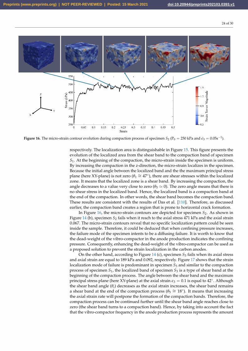
Figure 16. The micro-strain contour evolution during compaction process of specimen S2 (P0 = 250 kPa and ǫ3 = 0.05s−1).
respectively. The localization area is distinguishable in Figure 15. This figure presents theevolution of the localized area from the shear band to the compaction band of specimenS1. At the beginning of the compaction, the micro-strain inside the specimen is uniform.By increasing the compaction in the z-direction, the micro-strain localizes in the specimen.Because the initial angle between the localized band and the the maximum principal stressplane (here XY-plane) is not zero (θ1
∼= 47◦), there are shear stresses within the localizedzone. It means that the localized zone is a shear band. By increasing the compaction, theangle decreases to a value very close to zero (θ5 ≃ 0). The zero angle means that there isno shear stress in the localized band. Hence, the localized band is a compaction band atthe end of the compaction. In other words, the shear band becomes the compaction band.These results are consistent with the results of Das et al. [110]. Therefore, as discussedearlier, the compaction band creates a region that is prone to horizontal crack formation.
In Figure 16, the micro-strain contours are depicted for specimen S2. As shown inFigure 14 (b), specimen S2 fails when it reach to the axial stress 471 kPa and the axial strain0.067. The micro-strain contours reveal that no specific localization pattern could be seeninside the sample. Therefore, it could be deduced that when confining pressure increases,the failure mode of the specimen intents to be a diffusing failure. It is worth to know thatthe dead-weight of the vibro-compactor in the anode production indicates the confiningpressure. Consequently, enhancing the dead-weight of the vibro-compactor can be used asa proposed solution to prevent the strain localization in the carbon anodes.
On the other hand, according to Figure 14 (c), specimen S3 fails when its axial stressand axial strain are equal to 189 kPa and 0.092, respectively. Figure 17 shows that the strainlocalization mode of failure is predominant in specimen S3 and similar to the compactionprocess of specimen S1, the localized band of specimen S3 is a type of shear band at thebeginning of the compaction process. The angle between the shear band and the maximumprincipal stress plane (here XY-plane) at the axial strain ǫ3 = 0.1 is equal to 42◦. Althoughthe shear band angle (θi) decreases as the axial strain increases, the shear band remainsa shear band at the end of the compaction process (θ5
∼= 18◦). It means that increasingthe axial strain rate will postpone the formation of the compaction bands. Therefore, thecompaction process can be continued further until the shear band angle reaches close tozero (the shear band turns to a compaction band). Hence, by taking into account the factthat the vibro-compactor frequency in the anode production process represents the amount
Preprints (www.preprints.org) | NOT PEER-REVIEWED | Posted: 15 March 2021 doi:10.20944/preprints202103.0393.v1

25 of 30
Figure 17. The micro-strain contour evolution during compaction process of specimen S3 (P0 = 100 kPa and ǫ3 = 0.15s−1).
of the axial strain rate, increasing the frequency can be a suggested solution to inhibit theformation of compaction bands in the anode production process.
5. Conclusions
This paper presents a theoretical aspect of the failure analysis in the granular materialand a numerical investigation to find the failure in the mono-sized spherical coke aggregateunder different compaction conditions. Some conclusions can be summarized as follows:
• It has been shown that the strain localization could happen in the carbon anodesduring the compaction process and if this localized zone be a type of the compactionband, it could be responsible for the crack generation under the stub-holes in thecarbon anodes. As the carbon anode paste behavior during the compaction process istoo complex for considering, the dry mono-sized spherical coke aggregates have beenexamined.
• Considering failure as a bifurcation from a quasi-static regime to a dynamical one, afailure criterion was inferred, and the notion of the bifurcation domain was specified.The relationship between the kinetic energy of the granular materials and the internaland external second-order work has been evolved. It has been shown that when thefailure occurred, the stresses which sense at the boundaries cannot reflect the realstress inside the material.
• Using the DEM simulation, the optimum number of particles which could representthe bulk material for the failure analysis is justified. Four criteria, including having amore uniform force path network, having a smother stress-strain diagram, repetitivebehavior of the RVE, and a higher chance of the capturing the strain localization, havebeen exploited. It has been proved that the RVE with 3000 particles could representthe bulk material behavior in the failure analysis.
• The second-order criterion was used for finding the failure threshold in the specimens.The evolution of the shear band to the compaction band was investigated. Moreover,the effect of the confining pressure and the strain rate on the failure of the specimenshave been studied. It revealed that by enhancing the confining pressure, the failuremode of the specimen would be of the diffusing type. However, by increasing thestrain rate, the mode of the failure would be the localized type. In addition, the strainrate could postpone the formation of the compaction band, which can generate asusceptible area for the crack generation. The results highlighted that increasing the
Preprints (www.preprints.org) | NOT PEER-REVIEWED | Posted: 15 March 2021 doi:10.20944/preprints202103.0393.v1

26 of 30
confining pressure and the axial strain rate could be suggested solutions for preventingthe localization or postponing the formation of the compaction bands in the carbonanode.
This article focuses on the study of the failure behavior of the dry mono-sized coke aggre-gates. However, the coke aggregates are very complex as they are composed of particles ofdifferent sizes, different shapes, different materials, etc. In the next step, the role of the sizedistribution and particle shape on the failure of the coke aggregates will be explored byusing DEM simulation.
Appendix A
Let us consider, at a given time t, a homogeneous granular assembly of volume Vin equilibrium under prescribed boundary conditions. Then, the rate of the deformationgradient tensor can be obtained as [97]:
F = ∇v F. (A1)
In the other hand, we can use a pull-back transportation to bring the differential from thespatial configuration to the material configuration as:
∇v =∂v
∂X
∂X
∂x=
∂v
∂XF−1. (A2)
By substituting Equation (A2) in (A1), it comes:
F =
(∂v
∂XF−1
)
F =∂v
∂X. (A3)
Then, the mean value of the rate of the deformation gradient tensor (⟨
Fij
⟩) by using Green
formula is equal to:
⟨Fij
⟩=
1V0
∫∫∫
V0
∂vi
∂XjdV0
=1
V0
∫∫
S0
vi NidS0
=Aiui
V0. (A4)
Appendix B
By using a similar process, we can calculate the second rate of the deformation gradienttensor by using a time derivative of Equation (A3):
F =∂
∂t
(∂v
∂X
)
(A5)
Because X is independent of t, it can be written:
F =∂
∂X
(∂v
∂t
)
. (A6)
Then, by using Green formula, the mean value of the second rate of the deformationgradient tensor (
⟨Fij
⟩) is equal to:
⟨Fij
⟩=
1V0
∫∫∫
V0
∂
∂Xj
(∂vi
∂t
)
dV0
=1
V0
∫∫
S0
(∂vi
∂t
)
· Nj dS0
=Aiui
V0. (A7)
Author Contributions: Conceptualization, methodology, investigation, and writing—original draftpreparation, A.S.C.; Writing-review and editing, R.M., D.P., J.T., S.M.T, and H.A.; supervision, H.A.;All authors have read and agreed to the published version of the manuscript
Preprints (www.preprints.org) | NOT PEER-REVIEWED | Posted: 15 March 2021 doi:10.20944/preprints202103.0393.v1

27 of 30
Funding: A part of the research presented in this article was financed by the Fonds de recherche duQuébec – Nature et Technologies by the intermediary of the Aluminium Research Centre – REGAL.
Acknowledgments: The authors gratefully acknowledge the financial support provided by AlcoaInc., the Natural Sciences and Engineering Research Council of Canada and Centre Québécoisde Recherche et de Développement de l’Aluminium. We would like to express our very greatappreciation to Dr. Donald Ziegler for his valuable and constructive suggestions during the planningand development of this research work.
Conflicts of Interest: The authors declare no conflict of interest.
References
1. Welch, B.J. Aluminum production paths in the new millennium. JoM 1999, 51, 24–28. https://doi.org/10.1007/s11837-999-0036-4.2. Rhedey, P. A Review of factors affecting carbon anode consumption in the electrolytic production of aluminum. Essent. Read.
Light Met. 2016, pp. 611–622. https://doi.org/10.1007/978-3-319-48200-2_81.3. Hulse, K.L. Anode manufacture: raw materials, formulation and processing parameters; R& D Carbon Limited, 2000.4. Boubaker, M.B.; Picard, D.; Duchesne, C.; Tessier, J.; Alamdari, H.; Fafard, M. Non-destructive testing of baked anodes
based on modal analysis and principal component analysis. In Light Met.; Springer, Cham, 2017; pp. 1289–1298. https://doi.org/10.1007/978-3-319-51541-0_154.
5. Dorcheh, K.A. Investigation of the materials and paste relationships to improve forming process and anode quality. PhD thesis,Université Laval, Québec, Canada, 2013. http://hdl.handle.net/20.500.11794/24666.
6. Majidi, B. Discrete element method simulation of packing and rheological properties of coke and coke/pitch mixtures. PhDthesis, Université Laval, Québec, Canada, 2018. http://hdl.handle.net/20.500.11794/30959.
7. Azari, K.; Alamdari, H.; Ammar, H.; Fafard, M.; Adams, A.; Ziegler, D. Influence of mixing parameters on the density andcompaction behavior of carbon anodes used in aluminum production. Adv. Mat. Res. Trans. Tech. Publ., 2012, Vol. 409, pp.17–22. https://doi.org/10.4028/www.scientific.net/AMR.409.17.
8. Amrani, S.; Kocaefe, D.; Kocaefe, Y.; Morais, B.; Blaney, G. Effect of heating rate on the crack formation during baking in carbonanodes used in aluminum industry. In Light Met.; Springer, Cham, 2014; pp. 1175–1180. https://doi.org/10.1007/978-3-319-48144-9_196.
9. Amrani, S.; Kocaefe, D.; Kocaefe, Y.; Bhattacharyay, D.; Bouazara, M.; Morais, B. Characterization of cracking mechanisms ofcarbon anodes used in aluminum industry by optical microscopy and tomography. J. Mater. Eng. Perform. 2016, 25, 4274–4282.https://doi.org/10.1007/s11665-016-2257-3.
10. Chamam, Y.; Kocaefe, D.; Kocaefe, Y.; Bhattacharyay, D.; Morais, B. Effect of heating rate during baking on the properties ofcarbon anodes used in aluminum industry. In Light Met.; Springer, Cham, 2016; pp. 947–951. https://doi.org/10.1007/978-3-319-48251-4_159.
11. Menard, Y. Prebaked anode cracking and forming–reasons and solutions. Proceedings of 35th International ICSOBA Conference,Hamburg, Germany, 2017, pp. 2–5.
12. Amrani, S.; Kocaefe, D.; Kocaefe, Y.S.; Bhattacharyay, D.; Bouazara, M.; Coulombe, P. Evolution of anode properties duringbaking. Int. J. Innov. Sci. Eng. Technol. 2017, 4, 301–309.
13. Meier, M.W. Cracking behaviour of anodes; R & D Carbon, 1996.14. Schneider, J.; Coste, B. Thermomechanical modelling of thermal shock in anodes. Light Met. 1993, pp. 621–628.15. Chaouki, H.; Picard, D.; Ziegler, D.; Azari, K.; Alamdari, H.; Fafard, M. Viscoplastic modeling of the green anode paste compaction
process. J. Appl. Mech. 2016, 83. https://doi.org/10.1115/1.4031857.16. Anderson, T.L. Fracture mechanics: fundamentals and applications; CRC press, 2017. https://doi.org/10.1201/9781315370293.17. Chaouki, H.; Thibodeau, S.; Fafard, M.; Ziegler, D.; Alamdari, H. Characterization of the Hot Anode Paste Compaction Process:
A Computational and Experimental Study. Materials 2019, 12, 800. https://doi.org/10.3390/ma12050800.18. Andrade, J.E.; Avila, C.; Hall, S.; Lenoir, N.; Viggiani, G. Multiscale modeling and characterization of granular matter: from grain
kinematics to continuum mechanics. J. Mech. Phys. Solids 2011, 59, 237–250. https://doi.org/10.1016/j.jmps.2010.10.009.19. Majidi, B.; Melo, J.; Fafard, M.; Ziegler, D.; Alamdari, H. Packing density of irregular shape particles: DEM simulations applied to
anode-grade coke aggregates. Adv. Powder Technol. 2015, 26, 1256–1262. https://doi.org/10.1016/j.apt.2015.06.008.20. Majidi, B.; Rouget, G.; Fafard, M.; Ziegler, D.; Alamdari, H. Discrete element method investigation of bulk density and electrical
resistivity of calcined coke mixes. Metals 2017, 7, 154. https://doi.org/10.3390/met7050154.21. Rouget, G.; Majidi, B.; Picard, D.; Gauvin, G.; Ziegler, D.; Mashreghi, J.; Alamdari, H. Electrical resistivity measurement of
petroleum coke powder by means of four-probe method. Metall. Mater. Trans. B 2017, 48, 2543–2550. https://doi.org/10.1007/s11663-017-1022-9.
22. Daouadji, A.; Darve, F.; Al Gali, H.; Hicher, P.; Laouafa, F.; Lignon, S.; Nicot, F.; Nova, R.; Pinheiro, M.; Prunier, F.; Sibille, L.; Wan,R. Diffuse failure in geomaterials: Experiments, theory and modelling. Int. J. Numer. Anal. Methods Geomech. 2011, 35, 1731–1773.https://doi.org/10.1002/nag.975.
23. Nicot, F.; Sibille, L.; Darve, F. Failure in Granular Materials: Macro and Micro Views. In Bifurcations, Instabilities and Degradations
in Geomaterials; Springer, 2011; pp. 1–12. https://doi.org/10.1007/978-3-642-18284-6_1.
Preprints (www.preprints.org) | NOT PEER-REVIEWED | Posted: 15 March 2021 doi:10.20944/preprints202103.0393.v1

28 of 30
24. Nicot, F.; Darve, F. Diffuse and localized failure modes: two competing mechanisms. Int. J. Numer. Anal. Methods Geomech. 2011,35, 586–601. https://doi.org/10.1002/nag.912.
25. Sibille, L.; Hadda, N.; Nicot, F.; Tordesillas, A.; Darve, F. Granular plasticity, a contribution from discrete mechanics. J. Mech.
Phys. Solids 2015, 75, 119–139. https://doi.org/10.1016/j.jmps.2014.09.010.26. Hadda, N.; Sibille, L.; Nicot, F.; Wan, R.; Darve, F. Failure in granular media from an energy viewpoint. Granul. Matter 2016,
18, 50. https://doi.org/10.1007/s10035-016-0639-8.27. Chu, J.; Leong, W.; Loke, W.; Wanatowski, D. Instability of loose sand under drained conditions. J. Geotech. Geoenviron. Eng. 2012,
138, 207–216. https://doi.org/10.1061/(ASCE)GT.1943-5606.0000574.28. Simitses, G.; Hodges, D.H. Fundamentals of structural stability; Butterworth-Heinemann, 2006.29. Tordesillas, A.; Muthuswamy, M. On the modeling of confined buckling of force chains. J. Mech. Phys. Solids 2009, 57, 706–727.
https://doi.org/10.1016/j.jmps.2009.01.005.30. Ziegler, H. Principles of structural stability; Vol. 35, Birkhäuser, 2013.31. Wan, R.; Pinheiro, M.; Daouadji, A.; Jrad, M.; Darve, F. Diffuse instabilities with transition to localization in loose granular
materials. Int. J. Numer. Anal. Methods Geomech. 2013, 37, 1292–1311. https://doi.org/10.1002/nag.2085.32. Oda, M.; Kazama, H. Microstructure of shear bands and its relation to the mechanisms of dilatancy and failure of dense granular
soils. Geotechnique 1998, 48, 465–481. https://doi.org/10.1680/geot.1998.48.4.465.33. Darve, F.; Flavigny, E.; Meghachou, M. Constitutive modelling and instabilities of soil behaviour. Comput. Geotech. 1995,
17, 203–224. https://doi.org/10.1016/0266-352X(95)93869-K.34. Liapounoff, A. Problème général de la stabilité du mouvement. Annales de la Faculté des sciences de Toulouse: Mathématiques,
1907, Vol. 9, pp. 203–474. https://doi.org/10.5802/afst.246.35. Nova, R. Controllability of the incremental response of soil specimens subjected to arbitrary loading programmes. J. Mech. behav.
Mater. 1994, 5, 193–202. https://doi.org/10.1515/JMBM.1994.5.2.193.36. Nicot, F.; Darve, F.; Dat Vu Khoa, H. Bifurcation and second-order work in geomaterials. Int. J. Numer. Anal. Methods Geomech.
2007, 31, 1007–1032. https://doi.org/10.1002/nag.573.37. Chambon, R. Some theoretical results about second-order work, uniqueness, existence and controllability independent of the
constitutive equation. In Hill J. M., Selvadurai A. (eds) Mathematics and Mechanics of Granular Materials; Springer, Dordrecht, 2005;pp. 53–61. https://doi.org/10.1007/1-4020-4183-7_4.
38. Darve, F.; Laouafa, F. Instabilities in granular materials and application to landslides. Mech. Cohesive-frict. Mater. 2000, 5, 627–652.39. Nicot, F.; Darve, F. A micro-mechanical investigation of bifurcation in granular materials. Int. J. Solids Struct. 2007, 44, 6630–6652.
https://doi.org/10.1016/j.ijsolstr.2007.03.002.40. Hill, R. A general theory of uniqueness and stability in elastic-plastic solids. J. the Mech. Phys. Solids 1958, 6, 236–249.
https://doi.org/10.1016/0022-5096(58)90029-2.41. Darve, F.; Servant, G.; Laouafa, F.; Khoa, H. Failure in geomaterials: continuous and discrete analyses. Comput. Methods Appl.
Mech. Eng. 2004, 193, 3057–3085. https://doi.org/10.1016/j.cma.2003.11.011.42. Darve, F.; Sibille, L.; Daouadji, A.; Nicot, F. Bifurcations in granular media: macro-and micro-mechanics approaches. Comptes
Rendus Mécanique 2007, 335, 496–515. https://doi.org/10.1016/j.crme.2007.08.005.43. Lade, P.V. Instability, shear banding, and failure in granular materials. Int. J.Solids Struct. 2002, 39, 3337–3357.44. Rice, J.R.; Rudnicki, J. A note on some features of the theory of localization of deformation. Int. J. Solids Struct. 1980, 16, 597–605.
https://doi.org/10.1016/0020-7683(80)90019-0.45. Aydin, A.; Borja, R.I.; Eichhubl, P. Geological and mathematical framework for failure modes in granular rock. J. Struct. Geol.
2006, 28, 83–98. https://doi.org/10.1016/j.jsg.2005.07.008.46. Rudnicki, J.W.; Rice, J. Conditions for the localization of deformation in pressure-sensitive dilatant materials. J. Mech. Phys. Solids
1975, 23, 371–394. https://doi.org/10.1016/0022-5096(75)90001-0.47. Borja, R.I. Bifurcation of elastoplastic solids to shear band mode at finite strain. Comput. Methods Appl. Mech. Eng. 2002,
191, 5287–5314. https://doi.org/10.1016/S0045-7825(02)00459-0.48. Borja, R.I.; Aydin, A. Computational modeling of deformation bands in granular media. I. Geological and mathematical
framework. Comput. Methods Appl. Mech. Eng. 2004, 193, 2667–2698. https://doi.org/10.1016/j.cma.2003.09.019.49. Calvetti, F.; Combe, G.; Lanier, J. Experimental micromechanical analysis of a 2D granular material: relation between structure
evolution and loading path. Mech. Cohes. frict. Mater. 1997, 2, 121–163.50. Bésuelle, P.; Desrues, J.; Raynaud, S. Experimental characterisation of the localisation phenomenon inside a Vosges sandstone in a
triaxial cell. Int. J. Rock Mech. Min. Sci. 2000, 37, 1223–1237. https://doi.org/10.1016/S1365-1609(00)00057-5.51. Desrues, J.; Viggiani, G. Strain localization in sand: an overview of the experimental results obtained in Grenoble using
stereophotogrammetry. Int. J. Numer. Anal. Methods Geomech. 2004, 28, 279–321. https://doi.org/10.1002/nag.338.52. Zhuang, L.; Nakata, Y.; Kim, U.G.; Kim, D. Influence of relative density, particle shape, and stress path on the plane strain
compression behavior of granular materials. Acta Geotech. 2014, 9, 241–255. https://doi.org/10.1007/s11440-013-0253-4.53. Wu, K.; Pizette, P.; Becquart, F.; Remond, S.; Abriak, N.; Xu, W.; Liu, S. Experimental and numerical study of cylindrical
triaxial test on mono-sized glass beads under quasi-static loading condition. Adv. Powder Technol. 2017, 28, 155–166. https://doi.org/10.1016/j.apt.2016.09.006.
Preprints (www.preprints.org) | NOT PEER-REVIEWED | Posted: 15 March 2021 doi:10.20944/preprints202103.0393.v1

29 of 30
54. Alikarami, R.; Andò, E.; Gkiousas-Kapnisis, M.; Torabi, A.; Viggiani, G. Strain localisation and grain breakage in sand undershearing at high mean stress: insights from in situ X-ray tomography. Acta Geotech. 2015, 10, 15–30. https://doi.org/10.1144/SP289.4.
55. Borja, R.I. Computational modeling of deformation bands in granular media. II. Numerical simulations. Comput. Methods Appl.
Mech. Eng. 2004, 193, 2699–2718. https://doi.org/10.1016/j.cma.2003.09.018.56. Andrade, J.E.; Borja, R.I. Capturing strain localization in dense sands with random density. Int. J. Numer. Methods Eng. 2006,
67, 1531–1564. https://doi.org/10.1002/nme.1673.57. Wang, B.; Chen, Y.; Wong, T.f. A discrete element model for the development of compaction localization in granular rock. J.
Geophys. Res. Solid Earth 2008, 113. https://doi.org/10.1029/2006JB004501.58. Guo, N.; Zhao, J. 3D multiscale modeling of strain localization in granular media. Comput. Geotech. 2016, 80, 360–372.
https://doi.org/10.1016/j.compgeo.2016.01.020.59. Liang, W.; Zhao, J. Multiscale modeling of large deformation in geomechanics. Int. J. Numer. Anal. Methods Geomech. 2019,
43, 1080–1114. https://doi.org/10.1002/nag.2921.60. Alshibli, K.A.; Alsaleh, M.I.; Voyiadjis, G.Z. Modelling strain localization in granular materials using micropolar theory:
Numerical implementation and verification. Int. J Numer. Anal. Methods Geomech. 2006, 30, 1525–1544. https://doi.org/10.1002/nag.534.
61. De Borst, R. Simulation of strain localization: a reappraisal of the Cosserat continuum. Eng. Comput. 1991. https://doi.org/10.1108/eb023842.
62. Tang, H.; Dong, Y.; Wang, T.; Dong, Y. Simulation of strain localization with discrete element-Cosserat continuum finite elementtwo scale method for granular materials. J. Mech. Phys. Solids 2019, 122, 450–471. https://doi.org/10.1016/j.jmps.2018.09.029.
63. Scholtès, L.; Donzé, F.V. A DEM model for soft and hard rocks: role of grain interlocking on strength. J. Mech. Phys. Solids 2013,61, 352–369. https://doi.org/10.1016/j.jmps.2012.10.005.
64. Liu, Y.; Sun, W.; Yuan, Z.; Fish, J. A nonlocal multiscale discrete-continuum model for predicting mechanical behavior of granularmaterials. Int. J. Numer. Methods Eng. 2016, 106, 129–160. https://doi.org/10.1002/nme.5139.
65. Wu, H.; Zhao, J.; Liang, W. Pattern transitions of localized deformation in high-porosity sandstones: Insights from multiscaleanalysis. Comput. Geotech. 2020, 126, 103733. https://doi.org/10.1016/j.compgeo.2020.103733.
66. Khoa, H.D.V.; Georgopoulos, I.O.; Darve, F.; Laouafa, F. Diffuse failure in geomaterials: Experiments and modelling. Comput.
Geotech. 2006, 33, 1–14. https://doi.org/10.1016/j.compgeo.2006.01.002.67. Lade, P.V. Static instability and liquefaction of loose fine sandy slopes. J. Geotech. Eng. 1992, 118, 51–71. https://doi.org/10.1061/
(asce)0733-9410(1992)118:1(51).68. Chu, J.; Leroueil, S.; Leong, W. Unstable behaviour of sand and its implication for slope instability. Can. Geotech. J. 2003,
40, 873–885. https://doi.org/10.1139/t03-039.69. Borja, R.I. Conditions for instabilities in collapsible solids including volume implosion and compaction banding. Acta Geotech.
2006, 1, 107–122. https://doi.org/10.1007/s11440-006-0012-x.70. Sun, W. A unified method to predict diffuse and localized instabilities in sands. Geomech. Geoeng. 2013, 8, 65–75. https:
//doi.org/10.1080/17486025.2012.695403.71. Borja, R.I. Localized and diffuse bifurcations in porous rocks undergoing shear localization and cataclastic flow. In: Oñate
E., Owen R. (eds) Computational Plasticity, Comput. Methods Appl. Sci. Springer, Dordrecht, 2007, Vol. 7, pp. 37–53.https://doi.org/10.1007/978-1-4020-6577-4_3.
72. Borja, R.I. Condition for liquefaction instability in fluid-saturated granular soils. Acta Geotech. 2006, 1, 211. https://doi.org/10.1007/s11440-006-0017-5.
73. Andrade, J.E. A predictive framework for liquefaction instability. Géotechnique 2009, 59, 673–682. https://doi.org/10.1680/geot.7.00087.
74. Sibille, L.; Donzé, F.V.; Nicot, F.; Chareyre, B.; Darve, F. From bifurcation to failure in a granular material: a DEM analysis. Acta
Geotech. 2008, 3, 15. https://doi.org/10.1007/s11440-007-0035-y.75. Aydin, A.; Johnson, A.M. Analysis of faulting in porous sandstones. J. Struct. Geol. 1983, 5, 19–31. https://doi.org/10.1016/0191
-8141(83)90004-4.76. Aydin, A. Small faults formed as deformation bands in sandstone. In Rock Friction and Earthquake Prediction; Springer, 1978; pp.
913–930. https://doi.org/10.1007/978-3-0348-7182-2_22.77. Davatzes, N.C.; Aydin, A.; Eichhubl, P. Overprinting faulting mechanisms during the development of multiple fault sets in
sandstone, Chimney Rock fault array, Utah, USA. Tectonophysics 2003, 363, 1–18. https://doi.org/10.1016/S0040-1951(02)00647-9.78. Antonellini, M.A.; Aydin, A.; Pollard, D.D. Microstructure of deformation bands in porous sandstones at Arches National Park,
Utah. J. Struct. Geol. 1994, 16, 941–959. https://doi.org/10.1016/0191-8141(94)90077-9.79. Sternlof, K.R.; Karimi-Fard, M.; Pollard, D.; Durlofsky, L. Flow and transport effects of compaction bands in sandstone at scales
relevant to aquifer and reservoir management. Water Resour. Res. 2006, 42. https://doi.org/10.1029/2005WR004664.80. Mollema, P.; Antonellini, M. Compaction bands: a structural analog for anti-mode I cracks in aeolian sandstone. Tectonophysics
1996, 267, 209–228. https://doi.org/10.1016/S0040-1951(96)00098-4.81. Sternlof, K.R.; Rudnicki, J.W.; Pollard, D.D. Anticrack inclusion model for compaction bands in sandstone. J. Geophys. Res. B
2005, 110. https://doi.org/10.1029/2005JB003764.
Preprints (www.preprints.org) | NOT PEER-REVIEWED | Posted: 15 March 2021 doi:10.20944/preprints202103.0393.v1

30 of 30
82. Holcomb, D.; Rudnicki, J.W.; Issen, K.A.; Sternlof, K. Compaction localization in the Earth and the laboratory: state of the researchand research directions. Acta Geotech. 2007, 2, 1–15. https://doi.org/10.1007/s11440-007-0027-y.
83. Issen, K.; Casey, T.; Dixon, D.; Richards, M.; Ingraham, J. Characterization and modeling of localized compaction in aluminumfoam. Scr. Mater. 2005, 52, 911–915. https://doi.org/10.1016/j.scriptamat.2004.12.031.
84. Bastawros, A.; Bart-Smith, H.; Evans, A. Experimental analysis of deformation mechanisms in a closed-cell aluminum alloy foam.J. Mech. Phys. Solids 2000, 48, 301–322. https://doi.org/10.1016/S0022-5096(99)00035-6.
85. Park, C.; Nutt, S. Anisotropy and strain localization in steel foam. Mat. Sci. Eng. A 2001, 299, 68–74. https://doi.org/10.1016/S0921-5093(00)01418-0.
86. Papka, S.D.; Kyriakides, S. In-plane crushing of a polycarbonate honeycomb. Int. J. Solids Struct. 1998, 35, 239–267. https://doi.org/10.1016/S0020-7683(97)00062-0.
87. Eshelby, J.D. The determination of the elastic field of an ellipsoidal inclusion, and related problems. Proc. R. Soc. Lond. A-Math.
Phys. Eng. Sci. 1957, 241, 376–396. https://doi.org/10.1098/rspa.1957.0133.88. Katsman, R.; Aharonov, E.; Scher, H. Localized compaction in rocks: Eshelby’s inclusion and the spring network model. Geophys.
Res. Lett. 2006, 33. https://doi.org/10.1029/2005GL025628.89. Katsman, R.; Aharonov, E.; Scher, H. A numerical study on localized volume reduction in elastic media: some insights on the
mechanics of anticracks. J. Geophys. Res. B 2006, 111. https://doi.org/10.1029/2004JB003607.90. Katsman, R.; Aharonov, E. A study of compaction bands originating from cracks, notches, and compacted defects. J. Struct. Geol.
2006, 28, 508–518. https://doi.org/10.1016/j.jsg.2005.12.007.91. Thibodeau, S.; Alamdari, H.; Ziegler, D.P.; Fafard, M. New insight on the restructuring and breakage of particles during uniaxial
confined compression tests on aggregates of petroleum coke. Powder Technol. 2014, 253, 757–768. https://doi.org/10.1016/j.powtec.2013.12.048.
92. Nguyen, H.N.; Prunier, F.; Djeran-Maigre, I.; Nicot, F. Kinetic energy and collapse of granular materials. Granul. Matter 2016,18, 5. https://doi.org/10.1007/s10035-016-0609-1.
93. Nicot, F.; Sibille, L.; Darve, F. Failure in rate-independent granular materials as a bifurcation toward a dynamic regime. Int. J.
Plast. 2012, 29, 136–154. https://doi.org/10.1016/j.ijplas.2011.08.002.94. Hadda, N.; Nicot, F.; Bourrier, F.; Sibille, L.; Radjai, F.; Darve, F. Micromechanical analysis of second order work in granular
media. Granul. Matter 2013, 15, 221–235. https://doi.org/10.1007/s10035-013-0402-3.95. Holzapfel, A.G. Nonlinear solid mechanics: A continuum approach for engineering; John Wiley & Sons, Chichen., 2000. https:
//doi.org/10.1023/A:1020843529530.96. Nicot, F.; Hadda, N.; Bourrier, F.; Sibille, L.; Wan, R.; Darve, F. Inertia effects as a possible missing link between micro and macro
second-order work in granular media. Int. J. Solids Struct. 2012, 49, 1252–1258. https://doi.org/10.1016/j.ijsolstr.2012.02.005.97. Basar, Y.; Weichert, D. Nonlinear continuum mechanics of solids: fundamental mathematical and physical concepts; Springer Science &
Business Media, 2013. https://doi.org/10.1007/978-3-662-04299-1.98. Cundall, P.A.; Strack, O.D. A discrete numerical model for granular assemblies. Geotechnique 1979, 29, 47–65. https://doi.org/10
.1680/geot.1979.29.1.47.99. Šmilauer, V.; Catalano, E.; Chareyre, B.; Dorofeenko, S.; Duriez, J.; Gladky, A.; Kozicki, J.; Modenese, C.; Scholtès, L.; Sibille, L.;
others. Yade documentation. The Yade Project 2015. http://yade-dem.org/doc/.100. He, X.; Wu, W.; Cai, G.; Qi, J.; Kim, J.R.; Zhang, D.; Jiang, M. Work–energy analysis of granular assemblies validates and calibrates
a constitutive model. Granul. Matter 2020, 22, 28. https://doi.org/10.1007/s10035-019-0990-7.101. Nicot, F.; Lerbet, J.; Darve, F. Second-order work criterion: from material point to boundary value problems. Acta Mech. 2017,
228, 2483–2498. https://doi.org/10.1007/s00707-017-1844-1.102. Stroeven, M.; Askes, H.; Sluys, L. Numerical determination of representative volumes for granular materials. Comput. Methods
Appl. Mech. Eng. 2004, 193, 3221–3238. https://doi.org/10.1016/j.cma.2003.09.023.103. Evesque, P.; Adjemian, F. Stress fluctuations and macroscopic stick-slip in granular materials. Eur. Phys. J. E 2002, 9, 253–259.
https://doi.org/10.1140/epje/i2002-10082-4.104. Catalano, E.; Chareyre, B.; Barthélemy, E. Pore-scale modeling of fluid-particles interaction and emerging poromechanical effects.
Int. J. Numer. Anal. Methods Geomech. 2014, 38, 51–71. https://doi.org/10.1002/nag.2198.105. Bagi, K. Stress and strain in granular assemblies. Mech. Mater. 1996, 22, 165–178. https://doi.org/10.1016/0167-6636(95)00044-5.106. Bagi, K. Analysis of microstructural strain tensors for granular assemblies. Int. J. Solids Struct. 2006, 43, 3166–3184. https:
//doi.org/10.1016/j.ijsolstr.2005.07.016.107. Zhu, H.; Nguyen, H.N.; Nicot, F.; Darve, F. On a common critical state in localized and diffuse failure modes. J. Mech. Phys. Solids
2016, 95, 112–131. https://doi.org/10.1016/j.jmps.2016.05.026.108. Bardet, J.P. Numerical simulations of the incremental responses of idealized granular materials. Int. J. Plast. 1994, 10, 879–908.
https://doi.org/10.1016/0749-6419(94)90019-1.109. Tordesillas, A.; Pucilowski, S.; Sibille, L.; Nicot, F.; Darve, F. Multiscale characterisation of diffuse granular failure. Philos. Mag.
2012, 92, 4547–4587. https://doi.org/10.1080/14786435.2012.715766.110. Das, A.; Tengattini, A.; Nguyen, G.D.; Viggiani, G.; Hall, S.A.; Einav, I. A thermomechanical constitutive model for cemented
granular materials with quantifiable internal variables. Part II–validation and localization analysis. J. Mech. Phys. Solids 2014,70, 382–405. https://doi.org/10.1016/j.jmps.2014.05.022.
Powered by TCPDF (www.tcpdf.org)Powered by TCPDF (www.tcpdf.org)Powered by TCPDF (www.tcpdf.org)Powered by TCPDF (www.tcpdf.org)
Preprints (www.preprints.org) | NOT PEER-REVIEWED | Posted: 15 March 2021 doi:10.20944/preprints202103.0393.v1