discrete choice - sas customer support knowledge base and community
TRANSCRIPT

Discrete Choice
Warren F. Kuhfeld
Abstract
Discrete choice modeling is a popular technique in marketing research, transportation, and other areas.It is used to help researchers understand people’s stated choice of alternative products and services.We discuss designing a choice experiment, preparing the questionnaire, inputting and processing thedata, performing the analysis, and interpreting the results.∗ Most of the discussion is on designing thechoice experiment.
Introduction
This chapter shows you how to use the multinomial logit model (McFadden 1974; Manski and McFadden1981; Louviere and Woodworth 1983) to investigate consumer’s stated choices. The multinomial logitmodel is an alternative to full-profile conjoint analysis that is extremely popular in marketing research(Louviere 1991; Carson et. al. 1994). Discrete choice analysis, using the multinomial logit model, issometimes referred to as “choice-based conjoint.” However, the discrete choice model is different from afull-profile conjoint model. Discrete choice analysis uses a nonlinear model and aggregate choice data,whereas full-profile conjoint analysis uses a linear model and individual-level rating or ranking data.
The design and analysis of a discrete choice experiment is explained in the context of a series examples.†
There are also several very basic introductory examples starting on page 127 in the introduction toexperimental design chapter, which starts on page 53. Be sure to read the design chapter beforeproceeding to the examples in this chapter. The examples are as follows:
• The candy example (page 289) is a first, very simple example that discusses the multinomial logitmodel, the input data, analysis, results, and computing the probability of choice.
• The fabric softener example (page 302) is a small, somewhat more realistic example that dis-cusses designing the choice experiment, randomization, generating the questionnaire, enteringand processing the data, analysis, results, probability of choice, and custom questionnaires.
∗Copies of this chapter (MR-2010F), the other chapters, sample code, and all of the macros are available on theWeb http://support.sas.com/resources/papers/tnote/tnote_marketresearch.html. Specifically, sample code is herehttp://support.sas.com/techsup/technote/mr2010f.sas. For help, please contact SAS Technical Support. See page25 for more information.This document would not be possible without the help of Randy Tobias who contributed to thediscussion of experimental design and Ying So who contributed to the discussion of analysis. Randy Tobias wrote PROCFACTEX and PROC OPTEX. Ying So wrote PROC PHREG. Warren F. Kuhfeld wrote PROC TRANSREG and all ofthe macros.
†All of the example data sets are artificially generated.
285

286 MR-2010F — Discrete Choice
• The first vacation example (page 339) is a larger, symmetric example (all factors have the samenumber of levels) that discusses designing the choice experiment, blocks, randomization, gener-ating the questionnaire, entering and processing the data, coding, and alternative-specific effects.
• The second vacation example (page 410) is a larger, asymmetric example (not all factors havethe same number of levels) that discusses designing the choice experiment, blocks, blocking anexisting design, interactions, generating the questionnaire, generating artificial data, reading,processing, and analyzing the data, aggregating the data to save time and memory.
• The brand choice example (page 444) is a small example that discusses the processing of aggregatedata, the mother logit model, and the likelihood function.
• The food product example (page 468) is a medium sized example that discusses asymmetry,coding, checking the design to ensure that all effects are estimable, price cross-effects, availabilitycross-effects, interactions, overnight design searches, modeling subject attributes, and designswhen balance is of primary importance.
• The drug allocation example (page 535) is a small example that discusses data processing forstudies where respondents potentially make multiple choices.
• The chair example (page 556) is a purely generic-attributes study, and it uses the %ChoicEffmacro to create experimental designs.
• The next example section (page 580) shows how to improve an existing design and augmenting adesign with some choice sets are fixed in advance.
• The last example section (page 595) discusses partial-profile designs and designs with restrictions.Also see page 1079 for an example of a choice design with a complicated set of restrictions.
This chapter relies heavily on a number of macros and procedures.
• The %MktRuns autocall macro suggests design sizes. See page 1159 for documentation.
• The %MktEx autocall macro generates designs for linear models. These designs are directly usedfor conjoint studies. After post-processing they can also be used as choice designs. They arealso used to make candidate sets for directly constructing choice designs. Most examples use the%MktEx macro in some capacity. See page 1017 for documentation.
• The %MktEval autocall macro evaluates linear model designs. See page 1012 for documentation.
• The %ChoicEff autocall macro both generates and evaluates choice designs. See page 806 fordocumentation.
• The autocall macros %MktKey, %MktRoll, %MktMerge, and %MktAllo prepare the data and designfor analysis. See pages 1090, 1153, 1125, and 956 for documentation.
• PROC TRANSREG codes our designs, which puts the data into the final form for analysis.
• The %PHChoice autocall macro customizes our displayed output. This macro uses PROC TEM-PLATE and ODS (Output Delivery System) to customize the output from PROC PHREG, whichfits the multinomial logit model. See page 1173 for documentation.
• The %MktBal macro makes perfectly balanced designs for main effects models. See page 959 fordocumentation.

MR-2010F — Discrete Choice 287
• The %MktBlock macro block a linear or choice design into sets of alternatives or choice sets. Seepage 979 for documentation.
• The %MktDups macro searches a design for duplicate runs or choice sets. See page 1004 fordocumentation.
• The %MktLab macro assigns variable names, labels and levels to experimental designs and addsan intercept. See page 1093 for documentation.
• The %MktOrth macro lists the orthogonal experimental designs that the %MktEx macro can pro-duce. See page 1128 for documentation.
• The %MktPPro macro makes certain partial-profile choice designs. See page 1145 for documenta-tion.
• The %MktBIBD macro makes balanced incomplete block designs, unbalanced block designs, andmore generally, incomplete block designs, which are useful in constructing certain partial-profiledesigns and MaxDiff designs. See page 963 for documentation.
• The %MktMDiff macro processes and analyzes data from MaxDiff (best-worst) studies. See page1105 for documentation.
All of these macros are distributed with SAS 9.2 as autocall macros (see page 803 for more informationabout autocall macros), however, you should get the latest versions of the macros from the Webhttp://support.sas.com/resources/papers/tnote/tnote_marketresearch.html.
Experimental Design
Experimental design is a fundamental component of choice modeling. A discrete choice experimentaldesign consists of sets of products, and subjects choose a product from each set. Often, the mostchallenging part of the entire study is making the design. There are many examples of making choicedesigns in this chapter. Before you read them, be sure to read the design chapter beginning on page 53.There are also a number of design examples with the macro documentation. After you become familiarwith the design chapter, you should check out the %ChoicEff macro examples starting on page 808.
Customizing the Multinomial Logit Output
You can fit the multinomial logit model for discrete choice experiments by using the SAS/STAT pro-cedure PHREG (proportional hazards regression), with the ties=breslow option. The likelihoodfunction for the multinomial logit model has the same form as a survival analysis model fit by PROCPHREG. PROC PHREG and its output are primarily designed for survival-analysis studies. Beforeyou fit the multinomial logit model with PROC PHREG, you can customize its output templates tomake them more appropriate for choice experiments by using the %PHChoice autocall macro. See page803 for information about autocall macros. You can run the following macro to customize PROCPHREG output:
%phchoice(on)
288 MR-2010F — Discrete Choice
The macro uses PROC TEMPLATE and ODS (Output Delivery System) to customize the output fromPROC PHREG. Running this step edits two of the PROC PHREG templates and stores copies in thesasuser library. The default templates that SAS provides are stored in the library sashelp.tmplmst.By default, if you modify a template, it is stored in the library sasuser.templat. By default, ODSsearches sasuser.templat for templates, and then it searches sashelp.tmplmst if it does not find therequested template in sasuser.templat. You can see the list of template libraries by submitting thefollowing statement:
ods path show;
The template changes made by the %PHChoice macro do not affect the numerical output from PROCPHREG, but they do change the format and some of the titles, labels, and column headers that areused to label the output. Note that these changes assume that each effect in the choice model has avariable label associated with it, so there is no need to display variable names. If you are coding withPROC TRANSREG, this is usually the case. These changes remain in effect until you delete them. Toreturn to the default output from PROC PHREG, run the following macro:
%phchoice(off)
More generally, you can run the following step to delete the entire sasuser.templat library of cus-tomized templates so that ODS uses only the SAS supplied templates:
proc datasets library=sasuser;delete templat(memtype=itemstor);run;
If you only use PROC PHREG for choice modeling, and if you do not delete the contents of thesasuser or the template library, you only have to run the %PHChoice macro once, and the templatechanges are there for all subsequent steps that use the same template library in the sasuser library.Alternatively, you can choose to run phchoice(on) before running PROC PHREG and phchoice(off)after you are done. If you plan on using PROC PHREG for survival analysis, you should be sure torun phchoice(off) first so that your output is labeled appropriately for a survival study. See page1173 for more information about the %PHChoice macro.

MR-2010F — Candy Example 289
Candy Example
We begin with a very simple introductory example. In this example, we discuss the multinomial logitmodel, data input and processing, analysis, results, interpretation, and probability of choice. Manyaspects of this example, the experimental design in particular, are simpler than almost all realisticchoice studies. Still, it is useful to start with a simple choice study with no experimental design issuesto consider. In this example, each of ten subjects is presented with eight different chocolate candiesand asked to choose one. The eight candies consist of the 23 combinations of dark or milk chocolate,soft or chewy center, and nuts or no nuts. Each subject saw all eight candies and made one choice.Experimental choice data such as these are typically analyzed with a multinomial logit model.
The Multinomial Logit Model
The multinomial logit model assumes that the probability that an individual will choose one of the malternatives, ci, from choice set C is
p(ci|C) =exp(U(ci))∑m
j=1 exp(U(cj))=
exp(xiβ)∑mj=1 exp(xjβ)
where xi is a vector of coded attributes and β is a vector of unknown attribute parameters. At theheart- of this formula is a linear part-worth utility function, xiβ (like a linear regression function, butwrapped in a more complicated nonlinear model). U(ci) = xiβ is the utility for alternative ci, whichis a linear function of the attributes. The probability that an individual will choose one of the malternatives, ci, from choice set C is the exponential of the utility of the alternative divided by the sumof all of the exponentiated utilities.
There are m = 8 attribute vectors in this example, one for each alternative. Let x = (Dark/Milk,Soft/Chewy, Nuts/No Nuts) where Dark/Milk = (1 = Dark, 0 = Milk), Soft/Chewy = (1 = Soft, 0 =Chewy), Nuts/No Nuts = (1 = Nuts, 0 = No Nuts). The eight attribute vectors are
x1 = (0 0 0) (Milk, Chewy, No Nuts)x2 = (0 0 1) (Milk, Chewy, Nuts )x3 = (0 1 0) (Milk, Soft, No Nuts)x4 = (0 1 1) (Milk, Soft, Nuts )x5 = (1 0 0) (Dark, Chewy, No Nuts)x6 = (1 0 1) (Dark, Chewy, Nuts )x7 = (1 1 0) (Dark, Soft, No Nuts)x8 = (1 1 1) (Dark, Soft, Nuts )
Say, hypothetically that β′ = (4 −2 1). That is, the part-worth utility for dark chocolate is 4, thepart-worth utility for soft center is −2, and the part-worth utility for nuts is 1. The utility for each ofthe combinations, xiβ, is as follows:

290 MR-2010F — Discrete Choice
U(Milk, Chewy, No Nuts) = 0× 4 + 0×−2 + 0× 1 = 0U(Milk, Chewy, Nuts ) = 0× 4 + 0×−2 + 1× 1 = 1U(Milk, Soft, No Nuts) = 0× 4 + 1×−2 + 0× 1 = -2U(Milk, Soft, Nuts ) = 0× 4 + 1×−2 + 1× 1 = -1U(Dark, Chewy, No Nuts) = 1× 4 + 0×−2 + 0× 1 = 4U(Dark, Chewy, Nuts ) = 1× 4 + 0×−2 + 1× 1 = 5U(Dark, Soft, No Nuts) = 1× 4 + 1×−2 + 0× 1 = 2U(Dark, Soft, Nuts ) = 1× 4 + 1×−2 + 1× 1 = 3
The denominator of the probability formula,∑m
j=1 exp(xjβ), is exp(0)+exp(1)+exp(−2)+exp(−1)+exp(4) + exp(5) + exp(2) + exp(3) = 234.707. The probability that each alternative is chosen,exp(xiβ)/
∑mj=1 exp(xjβ), is
p(Milk, Chewy, No Nuts) = exp(0) / 234.707 = 0.004p(Milk, Chewy, Nuts ) = exp(1) / 234.707 = 0.012p(Milk, Soft, No Nuts) = exp(-2) / 234.707 = 0.001p(Milk, Soft, Nuts ) = exp(-1) / 234.707 = 0.002p(Dark, Chewy, No Nuts) = exp(4) / 234.707 = 0.233p(Dark, Chewy, Nuts ) = exp(5) / 234.707 = 0.632p(Dark, Soft, No Nuts) = exp(2) / 234.707 = 0.031p(Dark, Soft, Nuts ) = exp(3) / 234.707 = 0.086
Note that even combinations with a negative or zero utility have a nonzero probability of choice.Also note that adding a constant to the utilities does not change the probability of choice, howevermultiplying by a constant will.
Probability of choice is a nonlinear and increasing function of utility. The plot produced by the followingsteps shows the relationship between utility and probability of choice for this hypothetical situation:
data x;do u = -2 to 5 by 0.1;
p = exp(u) / 234.707;output;end;
label p = ’Probability(Choice)’ u = ’Utility’;run;
proc sgplot data=x;title ’Probability of Choice as a Function of Utility’;series y=p x=u;run;

MR-2010F — Candy Example 291
This plot shows the function exp(−2) to exp(5), scaled into the range zero to one, the range of prob-ability values. For the small negative utilities, the probability of choice is essentially zero. As utilityincreases beyond two, the function starts rapidly increasing.
In this example, the chosen alternatives are x5, x6, x7, x5, x2, x6, x2, x6, x6, x6. Alternative x2 ischosen 2 times, x5 is chosen 2 times, x6 is chosen 5 times, and x7 is chosen 1 time. The choice modellikelihood for these data is the product of ten terms, one for each choice set for each subject. Eachterm consists of the probability that the chosen alternative is chosen. For each choice set, the utilitiesfor all of the alternatives enter into the denominator, and the utility for the chosen alternative entersinto the numerator. The choice model likelihood for these data is
LC =exp(x5β)[∑8
j=1 exp(xjβ)] × exp(x6β)[∑8
j=1 exp(xjβ)] × exp(x7β)[∑8
j=1 exp(xjβ)] × exp(x5β)[∑8
j=1 exp(xjβ)] ×
exp(x2β)[∑8j=1 exp(xjβ)
] × exp(x6β)[∑8j=1 exp(xjβ)
] × exp(x2β)[∑8j=1 exp(xjβ)
] × exp(x6β)[∑8j=1 exp(xjβ)
] ×exp(x6β)[∑8
j=1 exp(xjβ)] × exp(x6β)[∑8
j=1 exp(xjβ)]
=exp((2x2 + 2x5 + 5x6 + x7)β)[∑8
j=1 exp(xjβ)]10
292 MR-2010F — Discrete Choice
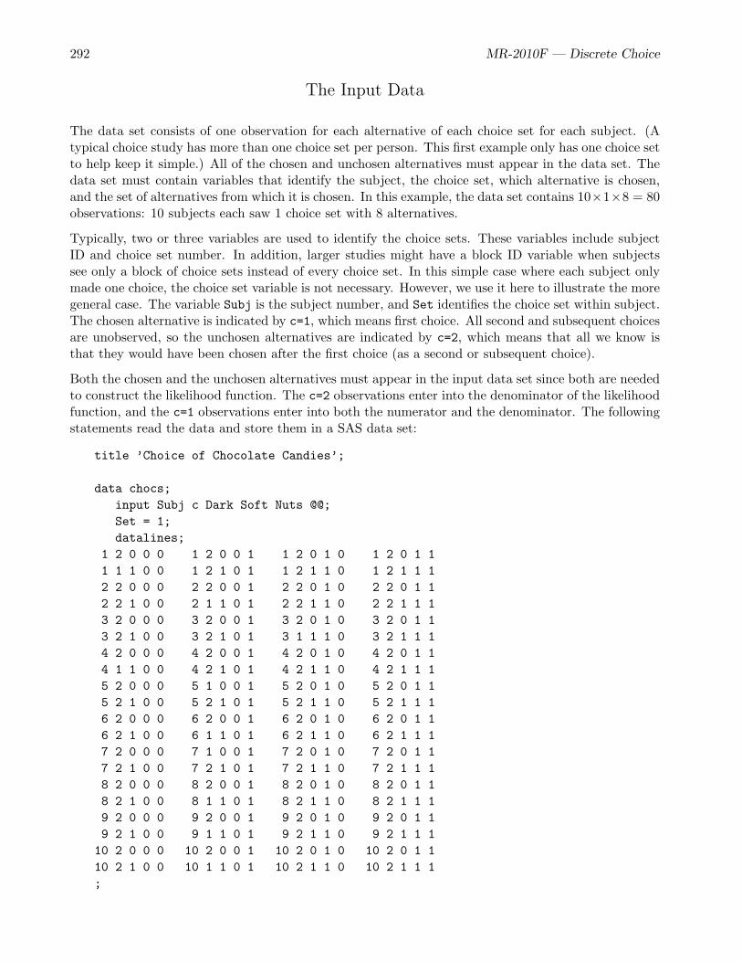
The Input Data
The data set consists of one observation for each alternative of each choice set for each subject. (Atypical choice study has more than one choice set per person. This first example only has one choice setto help keep it simple.) All of the chosen and unchosen alternatives must appear in the data set. Thedata set must contain variables that identify the subject, the choice set, which alternative is chosen,and the set of alternatives from which it is chosen. In this example, the data set contains 10×1×8 = 80observations: 10 subjects each saw 1 choice set with 8 alternatives.
Typically, two or three variables are used to identify the choice sets. These variables include subjectID and choice set number. In addition, larger studies might have a block ID variable when subjectssee only a block of choice sets instead of every choice set. In this simple case where each subject onlymade one choice, the choice set variable is not necessary. However, we use it here to illustrate the moregeneral case. The variable Subj is the subject number, and Set identifies the choice set within subject.The chosen alternative is indicated by c=1, which means first choice. All second and subsequent choicesare unobserved, so the unchosen alternatives are indicated by c=2, which means that all we know isthat they would have been chosen after the first choice (as a second or subsequent choice).
Both the chosen and the unchosen alternatives must appear in the input data set since both are neededto construct the likelihood function. The c=2 observations enter into the denominator of the likelihoodfunction, and the c=1 observations enter into both the numerator and the denominator. The followingstatements read the data and store them in a SAS data set:
title ’Choice of Chocolate Candies’;
data chocs;input Subj c Dark Soft Nuts @@;Set = 1;datalines;
1 2 0 0 0 1 2 0 0 1 1 2 0 1 0 1 2 0 1 11 1 1 0 0 1 2 1 0 1 1 2 1 1 0 1 2 1 1 12 2 0 0 0 2 2 0 0 1 2 2 0 1 0 2 2 0 1 12 2 1 0 0 2 1 1 0 1 2 2 1 1 0 2 2 1 1 13 2 0 0 0 3 2 0 0 1 3 2 0 1 0 3 2 0 1 13 2 1 0 0 3 2 1 0 1 3 1 1 1 0 3 2 1 1 14 2 0 0 0 4 2 0 0 1 4 2 0 1 0 4 2 0 1 14 1 1 0 0 4 2 1 0 1 4 2 1 1 0 4 2 1 1 15 2 0 0 0 5 1 0 0 1 5 2 0 1 0 5 2 0 1 15 2 1 0 0 5 2 1 0 1 5 2 1 1 0 5 2 1 1 16 2 0 0 0 6 2 0 0 1 6 2 0 1 0 6 2 0 1 16 2 1 0 0 6 1 1 0 1 6 2 1 1 0 6 2 1 1 17 2 0 0 0 7 1 0 0 1 7 2 0 1 0 7 2 0 1 17 2 1 0 0 7 2 1 0 1 7 2 1 1 0 7 2 1 1 18 2 0 0 0 8 2 0 0 1 8 2 0 1 0 8 2 0 1 18 2 1 0 0 8 1 1 0 1 8 2 1 1 0 8 2 1 1 19 2 0 0 0 9 2 0 0 1 9 2 0 1 0 9 2 0 1 19 2 1 0 0 9 1 1 0 1 9 2 1 1 0 9 2 1 1 110 2 0 0 0 10 2 0 0 1 10 2 0 1 0 10 2 0 1 110 2 1 0 0 10 1 1 0 1 10 2 1 1 0 10 2 1 1 1;

MR-2010F — Candy Example 293
In this DATA step, the data for four alternatives appear on one line, and all of the data for a choice setof eight alternatives appear on two lines. The DATA step shows the data entry in the way that requiresthe fewest programming statements. Each execution of the input statement reads information aboutone alternative. The @@ in the input statement specifies that SAS should not automatically go to anew input data set line when it reads the next row of data. This specification is needed here becauseeach line in the input data set contains the data for four output data set rows. The data from the firsttwo subjects is displayed as follows:
proc print data=chocs noobs;where subj <= 2;var subj set c dark soft nuts;run;
The data for the first two subjects is as follows:
Choice of Chocolate Candies
Subj Set c Dark Soft Nuts
1 1 2 0 0 01 1 2 0 0 11 1 2 0 1 01 1 2 0 1 11 1 1 1 0 01 1 2 1 0 11 1 2 1 1 01 1 2 1 1 12 1 2 0 0 02 1 2 0 0 12 1 2 0 1 02 1 2 0 1 12 1 2 1 0 02 1 1 1 0 12 1 2 1 1 02 1 2 1 1 1
These next steps illustrate a more typical form of data entry. The experimental design and the data arestored in separate data sets. Then they are merged and processed to produce the same results as thepreceding steps. The process of merging the experimental design and the data is explicitly illustratedhere with a DATA step program. In practice, and in all of the other examples, we use the %MktMergemacro to do this. The following steps read the design, merge it with the data, and designate first andsubsequent choices:

294 MR-2010F — Discrete Choice
title ’Choice of Chocolate Candies’;
* Alternative Form of Data Entry;
data combos; /* Read the design matrix. */input Dark Soft Nuts;datalines;
0 0 00 0 10 1 00 1 11 0 01 0 11 1 01 1 1;
data chocs; /* Create the data set. */input Choice @@; drop choice; /* Read the chosen combo num. */Subj = _n_; Set = 1; /* Store subj, choice set num. */do i = 1 to 8; /* Loop over alternatives. */
c = 2 - (i eq choice); /* Designate chosen alt. */set combos point=i; /* Read design matrix. */output; /* Output the results. */end;
datalines;5 6 7 5 2 6 2 6 6 6;
The variable Choice is the number of the chosen alternative. For each choice set, each of the eightobservations in the experimental design is read. The point= option in the set statement is used toread the ith observation of the data set Combos. When i (the alternative index) equals Choice (thenumber of the chosen alternative), the logical expression (i eq choice) equals 1; otherwise it is 0.The statement c = 2 - (i eq choice) sets c to 1 (two minus one) when the alternative is chosenand 2 (two minus zero) otherwise. All eight observations in the Combos data set are read 10 times, onceper subject. The resulting data set is the same as the one we created previously. As we mentionedpreviously, in all of the remaining examples, we simplify this process by using the %MktMerge macroto merge the design and data and flag the chosen and unchosen alternatives. Still, it is good to knowwhat the %MktMerge step does. The basic logic underlying this macro is shown in the preceding step.The number of a chosen alternative is read, then each alternative of the choice set is read, the chosenalternative is flagged (c = 1), and the unchosen alternatives are flagged (c = 2). One observationper choice set per subject is read from the input data, and one observation per alternative per choiceset per subject is written.
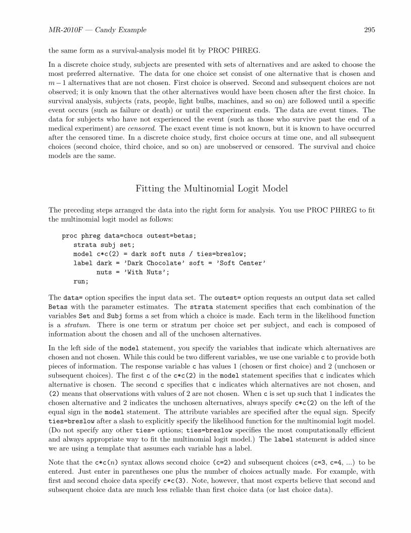
Choice and Survival Models
In SAS, the multinomial logit model is fit with the SAS/STAT procedure PHREG (proportional hazardsregression), with the ties=breslow option. The likelihood function of the multinomial logit model has
MR-2010F — Candy Example 295
the same form as a survival-analysis model fit by PROC PHREG.
In a discrete choice study, subjects are presented with sets of alternatives and are asked to choose themost preferred alternative. The data for one choice set consist of one alternative that is chosen andm−1 alternatives that are not chosen. First choice is observed. Second and subsequent choices are notobserved; it is only known that the other alternatives would have been chosen after the first choice. Insurvival analysis, subjects (rats, people, light bulbs, machines, and so on) are followed until a specificevent occurs (such as failure or death) or until the experiment ends. The data are event times. Thedata for subjects who have not experienced the event (such as those who survive past the end of amedical experiment) are censored. The exact event time is not known, but it is known to have occurredafter the censored time. In a discrete choice study, first choice occurs at time one, and all subsequentchoices (second choice, third choice, and so on) are unobserved or censored. The survival and choicemodels are the same.
Fitting the Multinomial Logit Model
The preceding steps arranged the data into the right form for analysis. You use PROC PHREG to fitthe multinomial logit model as follows:
proc phreg data=chocs outest=betas;strata subj set;model c*c(2) = dark soft nuts / ties=breslow;label dark = ’Dark Chocolate’ soft = ’Soft Center’
nuts = ’With Nuts’;run;
The data= option specifies the input data set. The outest= option requests an output data set calledBetas with the parameter estimates. The strata statement specifies that each combination of thevariables Set and Subj forms a set from which a choice is made. Each term in the likelihood functionis a stratum. There is one term or stratum per choice set per subject, and each is composed ofinformation about the chosen and all of the unchosen alternatives.
In the left side of the model statement, you specify the variables that indicate which alternatives arechosen and not chosen. While this could be two different variables, we use one variable c to provide bothpieces of information. The response variable c has values 1 (chosen or first choice) and 2 (unchosen orsubsequent choices). The first c of the c*c(2) in the model statement specifies that c indicates whichalternative is chosen. The second c specifies that c indicates which alternatives are not chosen, and(2) means that observations with values of 2 are not chosen. When c is set up such that 1 indicates thechosen alternative and 2 indicates the unchosen alternatives, always specify c*c(2) on the left of theequal sign in the model statement. The attribute variables are specified after the equal sign. Specifyties=breslow after a slash to explicitly specify the likelihood function for the multinomial logit model.(Do not specify any other ties= options; ties=breslow specifies the most computationally efficientand always appropriate way to fit the multinomial logit model.) The label statement is added sincewe are using a template that assumes each variable has a label.
Note that the c*c(n) syntax allows second choice (c=2) and subsequent choices (c=3, c=4, ...) to beentered. Just enter in parentheses one plus the number of choices actually made. For example, withfirst and second choice data specify c*c(3). Note, however, that most experts believe that second andsubsequent choice data are much less reliable than first choice data (or last choice data).

296 MR-2010F — Discrete Choice
Multinomial Logit Model Results
Recall that we specified %phchoice(on) on page 287 to customize the output from PROC PHREG.The results are as follows:
Choice of Chocolate Candies
The PHREG Procedure
Model Information
Data Set WORK.CHOCSDependent Variable cCensoring Variable cCensoring Value(s) 2Ties Handling BRESLOW
Number of Observations Read 80Number of Observations Used 80
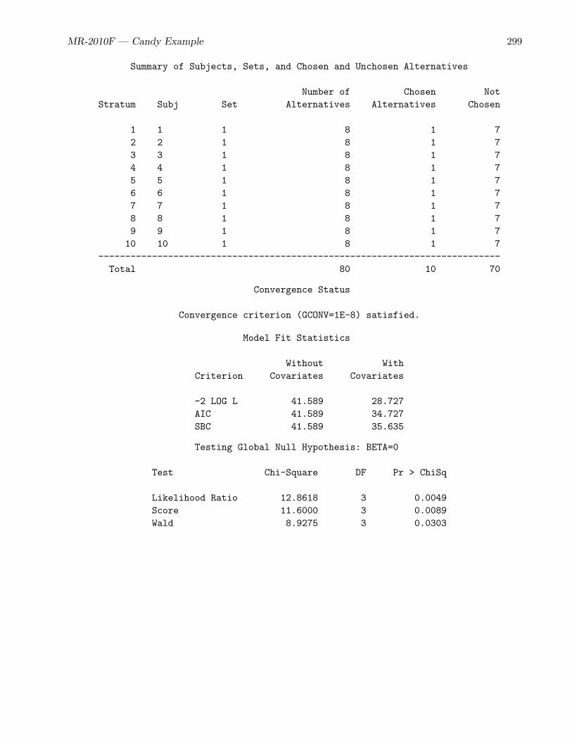
Summary of Subjects, Sets, and Chosen and Unchosen Alternatives
Number of Chosen NotStratum Subj Set Alternatives Alternatives Chosen
1 1 1 8 1 72 2 1 8 1 73 3 1 8 1 74 4 1 8 1 75 5 1 8 1 76 6 1 8 1 77 7 1 8 1 78 8 1 8 1 79 9 1 8 1 710 10 1 8 1 7
---------------------------------------------------------------------------Total 80 10 70
Convergence Status
Convergence criterion (GCONV=1E-8) satisfied.
Model Fit Statistics
Without WithCriterion Covariates Covariates
-2 LOG L 41.589 28.727AIC 41.589 34.727SBC 41.589 35.635

MR-2010F — Candy Example 297
Testing Global Null Hypothesis: BETA=0
Test Chi-Square DF Pr > ChiSq
Likelihood Ratio 12.8618 3 0.0049Score 11.6000 3 0.0089Wald 8.9275 3 0.0303
Choice of Chocolate Candies
The PHREG Procedure
Multinomial Logit Parameter Estimates
Parameter StandardDF Estimate Error Chi-Square Pr > ChiSq
Dark Chocolate 1 1.38629 0.79057 3.0749 0.0795Soft Center 1 -2.19722 1.05409 4.3450 0.0371With Nuts 1 0.84730 0.69007 1.5076 0.2195
The first table, Model Information, contains the input data set name, dependent variable name,censoring information, and tie handling option. The next table shows that 80 observations are readfrom the input SAS data set, and all 80 of them are used in the analysis.
The Summary of Subjects, Sets, and Chosen and Unchosen Alternatives table is displayed bydefault and should be used to check the data entry. There are as many strata as there are combinationsof the Subj and Set variables.∗ In this case, there are ten strata. Each stratum must be composed ofm alternatives. In this case, there are eight alternatives. The number of chosen alternatives should be1, and the number of unchosen alternatives is m− 1 (in this case, 7). Always check the summarytable to ensure that the data are arrayed correctly.
The Convergence Status table shows that the iterative algorithm successfully converged. The nexttables, Model Fit Statistics and Testing Global Null Hypothesis: BETA=0 contain the overallfit of the model. The –2 LOG L statistic under With Covariates is 28.727 and the Chi-Square statisticis 12.8618 with 3 df (p=0.0049), which is used to test the null hypothesis that the attributes do notinfluence choice. At common alpha levels such as 0.05 and 0.01, we reject the null hypothesis of norelationship between choice and the attributes. Note that 41.589 (–2 LOG L Without Covariates, whichis –2 LOG L for a model with no explanatory variables) minus 28.727 (–2 LOG L With Covariates,which is –2 LOG L for a model with all explanatory variables) equals 12.8618 (Model Chi-Square,which is used to test the effects of the explanatory variables).
The Multinomial Logit Parameter Estimates table is next. For each effect, it contains the maxi-mum likelihood parameter estimate, its estimated standard error (the square root of the correspondingdiagonal element of the estimated variance matrix), the Wald Chi-Square statistic (the square of theparameter estimate divided by its standard error), the df of the Wald Chi-Square statistic (1 unless thecorresponding parameter is redundant or infinite, in which case the value is 0), and the p-value of theChi-Squared statistic with respect to a chi-squared distribution with one df. The parameter estimate
∗More generally, there are as many strata as there are combinations of the Subj, Set, and block ID variable. In thiscase, there is only one block and no blocking variable.

298 MR-2010F — Discrete Choice
with the smallest p-value is for soft center. Since the parameter estimate is negative, chewy is the morepreferred level. Dark is preferred over milk, and nuts over no nuts, however only the p-value for Soft isless than 0.05.
Fitting the Multinomial Logit Model, All Levels
It is instructive to perform some manipulations on the data set and analyze it again. These stepsperform the same analysis as before, only now, coefficients for both levels of the three attributes aredisplayed:
data chocs2;set chocs;Milk = 1 - dark; Chewy = 1 - Soft; NoNuts = 1 - nuts;label dark = ’Dark Chocolate’ milk = ’Milk Chocolate’
soft = ’Soft Center’ chewy = ’Chewy Center’nuts = ’With Nuts’ nonuts = ’No Nuts’;
run;
proc phreg data=chocs2;strata subj set;model c*c(2) = dark milk soft chewy nuts nonuts / ties=breslow;run;
Binary variables for the missing levels are created by subtracting the existing binary variables from 1.The output is as follows:
Choice of Chocolate Candies
The PHREG Procedure
Model Information
Data Set WORK.CHOCS2Dependent Variable c
Censoring Variable cCensoring Value(s) 2Ties Handling BRESLOW
Number of Observations Read 80Number of Observations Used 80
MR-2010F — Candy Example 299
Summary of Subjects, Sets, and Chosen and Unchosen Alternatives
Number of Chosen NotStratum Subj Set Alternatives Alternatives Chosen
1 1 1 8 1 72 2 1 8 1 73 3 1 8 1 74 4 1 8 1 75 5 1 8 1 76 6 1 8 1 77 7 1 8 1 78 8 1 8 1 79 9 1 8 1 710 10 1 8 1 7
---------------------------------------------------------------------------Total 80 10 70
Convergence Status
Convergence criterion (GCONV=1E-8) satisfied.
Model Fit Statistics
Without WithCriterion Covariates Covariates
-2 LOG L 41.589 28.727AIC 41.589 34.727SBC 41.589 35.635
Testing Global Null Hypothesis: BETA=0
Test Chi-Square DF Pr > ChiSq
Likelihood Ratio 12.8618 3 0.0049Score 11.6000 3 0.0089Wald 8.9275 3 0.0303

300 MR-2010F — Discrete Choice
Choice of Chocolate Candies
The PHREG Procedure
Multinomial Logit Parameter Estimates
Parameter StandardDF Estimate Error Chi-Square Pr > ChiSq
Dark Chocolate 1 1.38629 0.79057 3.0749 0.0795Milk Chocolate 0 0 . . .Soft Center 1 -2.19722 1.05409 4.3450 0.0371Chewy Center 0 0 . . .With Nuts 1 0.84730 0.69007 1.5076 0.2195No Nuts 0 0 . . .
Now, the zero coefficients for the reference levels, milk, chewy, and no nuts are displayed. The part-worth utility for Milk Chocolate is a structural zero, and the part-worth utility for Dark Chocolateis larger at 1.38629. Similarly, the part-worth utility for Chewy Center is a structural zero, and thepart-worth utility for Soft Center is smaller at −2.19722. Finally, the part-worth utility for No Nuts isa structural zero, and the part-worth utility for Nuts is larger at 0.84730.
Probability of Choice
The parameter estimates are used next to construct the estimated probability that each alternative ischosen. The DATA step program uses the following formula to create the choice probabilities:
p(ci|C) =exp(xiβ)∑m
j=1 exp(xjβ)
* Estimate the probability that each alternative is chosen;
data p;retain sum 0;set combos end=eof;
* On the first pass through the DATA step (_n_ is the passnumber), get the regression coefficients in B1-B3.Note that they are automatically retained so that theycan be used in all passes through the DATA step.;
if _n_ = 1 thenset betas(rename=(dark=b1 soft=b2 nuts=b3));
keep dark soft nuts p;array x[3] dark soft nuts;array b[3] b1-b3;

MR-2010F — Candy Example 301
* For each combination, create x * b;p = 0;do j = 1 to 3;
p = p + x[j] * b[j];end;
* Exponentiate x * b and sum them up;p = exp(p);sum = sum + p;
* Output sum exp(x * b) to the macro variable ’&sum’;if eof then call symputx(’sum’, sum);run;
proc format;value df 1 = ’Dark’ 0 = ’Milk’;value sf 1 = ’Soft’ 0 = ’Chewy’;value nf 1 = ’Nuts’ 0 = ’No Nuts’;run;
* Divide each exp(x * b) by sum exp(x * b);data p;
set p;p = p / (&sum);format dark df. soft sf. nuts nf.;run;
proc sort;by descending p;run;
proc print;run;
The results are as follows:
Choice of Chocolate Candies
Obs Dark Soft Nuts p
1 Dark Chewy Nuts 0.504002 Dark Chewy No Nuts 0.216003 Milk Chewy Nuts 0.126004 Dark Soft Nuts 0.056005 Milk Chewy No Nuts 0.054006 Dark Soft No Nuts 0.024007 Milk Soft Nuts 0.014008 Milk Soft No Nuts 0.00600
The three most preferred alternatives are Dark/Chewy/Nuts, Dark/Chewy/No Nuts, and Milk/Chewy/Nuts.

302 MR-2010F — Discrete Choice
Fabric Softener Example
In this example, subjects are asked to choose among fabric softeners. This example shows all of the stepsin a discrete choice study, including experimental design creation and evaluation, creating the ques-tionnaire, inputting the raw data, creating the data set for analysis, coding, fitting the discrete choicemodel, interpretation, and probability of choice. In addition, custom questionnaires are discussed. Weassume that you are familiar with the experimental design issues that are discussed starting on page53.
Set Up
The study involves four fictitious fabric softeners Sploosh, Plumbbob, Platter, and Moosey.∗ There are50 subjects, each of which see the same choice sets.
Each choice set consists of each of these four brands and a constant alternative Another. Each of thebrands is available at three prices, $1.49, $1.99, and $2.49. Another is only offered at $1.99. Thetotal number of alternatives for this study is four, since there are four brands, and each consists ofone attribute, namely price. Since the constant alternative does not vary, it does not enter into theexperimental design at this stage. We use an approach in this example that is discussed in detail in theexperimental design chapter starting on page 53. Namely, we start by making a “linear arrangementof a choice design,” with one factor for every attribute of every alternative, and use that to make ourfinal choice design.
We can use the %MktRuns autocall macro to help us choose the number of choice sets. All of the autocallmacros used in this book are documented starting on page 803. To use this macro, you specify thenumber of levels for each of the factors. With four price factors (one for each of the four brands) eachwith three prices, you specify four 3’s (or equivalently, 3 ** 4). The %MktRuns macro is invoked asfollows:
title ’Choice of Fabric Softener’;
%mktruns(3 3 3 3)
The output from this macro is as follows:
Choice of Fabric Softener
Design Summary
Number ofLevels Frequency
3 4
∗Of course real studies use real brands. We have not collected real data, so we cannot use real brand names withartificial data. We picked these silly names so no one would confuse our artificial data with real data.

MR-2010F — Fabric Softener Example 303
Choice of Fabric Softener
Saturated = 9Full Factorial = 81
Some Reasonable Cannot BeDesign Sizes Violations Divided By
9 *S 018 * 012 6 915 6 910 10 3 911 10 3 913 10 3 914 10 3 916 10 3 917 10 3 9
* - 100% Efficient design can be made with the MktEx macro.S - Saturated Design - The smallest design that can be made.
Choice of Fabric Softener
n Design Reference
9 3 ** 4 Fractional-Factorial18 2 ** 1 3 ** 7 Orthogonal Array18 3 ** 6 6 ** 1 Orthogonal Array
The output first tells us that we specified a design with four factors, each with three levels. The nexttable reports the size of the saturated design, which is the number of parameters in the linear modelbased on this design. After that, design sizes are suggested.
The output from this macro tells us that the saturated design has nine runs and the full-factorialdesign has 81 runs. It also tells us that 9 and 18 are optimal design sizes with zero violations. Themacro tells us that in nine runs, an orthogonal design with 4 three-level factors is available, and in 18runs, two orthogonal and balanced designs are available: one with a two-level factor and 7 three-levelfactors, and one with 6 three-level factors and a six-level factor. There are zero violations with thesedesigns because these sizes can be divided by 3 and 3 × 3 = 9. Twelve and 15 are also reported aspotential design sizes, but each has 6 violations. Six times (the 4(4−1)/2 = 6 pairs of the four 3’s) thedesign sizes of 12 and 15 cannot be divided by 3× 3 = 9. Ideally, we would like to have a manageablenumber of choice sets for people to evaluate and a design that is both orthogonal and balanced. Whenviolations are reported, orthogonal and balanced designs are not possible. While orthogonality andbalance are not required, they are nice properties to have. With 4 three-level factors, the number ofchoice sets in all orthogonal and balanced designs must be divisible by 3× 3 = 9.

304 MR-2010F — Discrete Choice
Nine choice sets is a bit small. Furthermore, there are no error df. We set the number of choice sets to18 since it is small enough for each person to see all choice sets, large enough to have reasonable errordf, and an orthogonal and balanced design is available. It is important to understand, however, thatthe concept of number of parameters and error df discussed here applies to the linear arrangement ofthe choice design and not to the choice model.∗ We could use the nine-run design for a discrete choicemodel and have error df in the choice model. If we were to instead use this design for a full-profileconjoint (not recommended), there would be no error df.
To make the code easier to modify for future use, the number of choice sets and alternatives are storedin macro variables and the prices are put into a format. Our design, in raw form, has values for priceof 1, 2, and 3. We use a format to assign the actual prices: $1.49, $1.99, and $2.49. The format alsocreates a price of $1.99 for missing, which is used for the constant alternative. The following statementscreate the macro variables and format:
%let n = 18; /* n choice sets */%let m = 5; /* m alternative including constant */%let mm1 = %eval(&m - 1); /* m - 1 */
proc format; /* create a format for the price */value price 1 = ’$1.49’ 2 = ’$1.99’ 3 = ’$2.49’ . = ’$1.99’;run;
Designing the Choice Experiment
The next step creates an efficient experimental design. We use the autocall macro %MktEx to createmany of our designs. (All of the autocall macros used in this book are documented starting on page803.) When you invoke the %MktEx macro for a simple problem, you only need to specify the numbersof levels and the number of runs. The macro does the rest. The %MktEx macro usage for this exampleis as follows:
%mktex(3 ** 4, n=&n)
The syntax ’n ** m’ means m factors each at n levels. This example has four factors, x1 through x4,all with three levels. The n= option specifies the number of runs. The specification n=&n is equivalentto n=18, and it requests a design in 18 runs. These are all the options that are needed for a simpleproblem such as this one. However, throughout this book, random number seeds are explicitly specifiedwith the seed= option so that the results are reproducible.∗ The macro call with the random numberseed specified is as follows:
%mktex(3 ** 4, n=&n, seed=17)
∗See page 67 for an explanation of the linear arrangement of a choice design versus the arrangement of a choice designthat is more suitable for analysis.
∗By specifying a random number seed, results should be reproducible within a SAS release for a particular operatingsystem and for a particular version of the macro. However, due to machine and macro differences, some results mightnot be exactly reproducible everywhere. For most orthogonal and balanced designs, the results should be reproducible.When computerized searches are done, it is likely that you will not get the same design as the one in the book, althoughyou would expect the efficiency differences to be slight.
MR-2010F — Fabric Softener Example 305
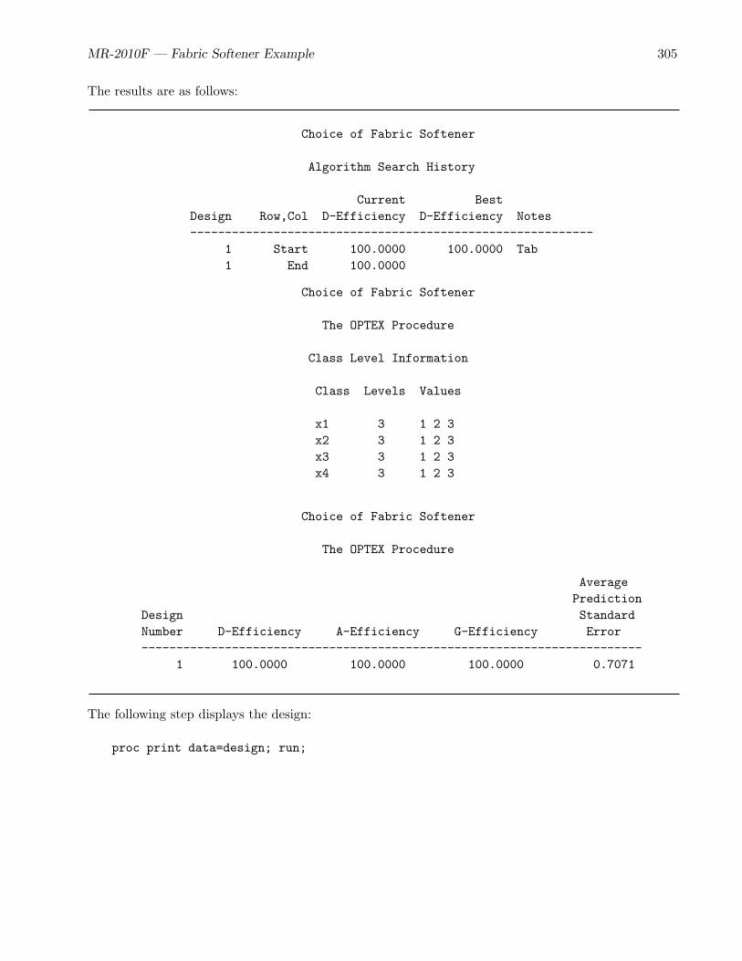
The results are as follows:
Choice of Fabric Softener
Algorithm Search History
Current BestDesign Row,Col D-Efficiency D-Efficiency Notes----------------------------------------------------------
1 Start 100.0000 100.0000 Tab1 End 100.0000
Choice of Fabric Softener
The OPTEX Procedure
Class Level Information
Class Levels Values
x1 3 1 2 3x2 3 1 2 3x3 3 1 2 3x4 3 1 2 3
Choice of Fabric Softener
The OPTEX Procedure
AveragePrediction
Design StandardNumber D-Efficiency A-Efficiency G-Efficiency Error------------------------------------------------------------------------
1 100.0000 100.0000 100.0000 0.7071
The following step displays the design:
proc print data=design; run;

306 MR-2010F — Discrete Choice
The design is as follows:
Choice of Fabric Softener
Obs x1 x2 x3 x4
1 1 1 1 12 1 1 2 23 1 2 1 34 1 2 3 15 1 3 2 36 1 3 3 27 2 1 1 38 2 1 3 19 2 2 2 210 2 2 3 311 2 3 1 212 2 3 2 113 3 1 2 314 3 1 3 215 3 2 1 216 3 2 2 117 3 3 1 118 3 3 3 3
The macro found a perfect, orthogonal and balanced, 100% D-efficient design consisting of 4 three-levelfactors, x1-x4. The levels are the integers 1 to 3. For this problem, the macro generated the designdirectly. For other problems, the macro might have to use a computerized search. See page 347 formore information about how the %MktEx macro works.
Examining the Design
You should run basic checks on all designs, even orthogonal designs such as this one. You can usethe %MktEval macro to display information about the design. The macro first displays a matrix ofcanonical correlations between the factors. We hope to see an identity matrix (a matrix of ones on thediagonal and zeros everywhere else) which means the design is orthogonal. Next, the macro displays allone-way frequencies for all attributes, all two-way frequencies, and all n-way frequencies (in this casefour-way frequencies). We hope to see equal or at least nearly equal one-way and two-way frequencies,and we want to see that each combination occurs only once. The following step creates the design:
%mkteval(data=design)
MR-2010F — Fabric Softener Example 307
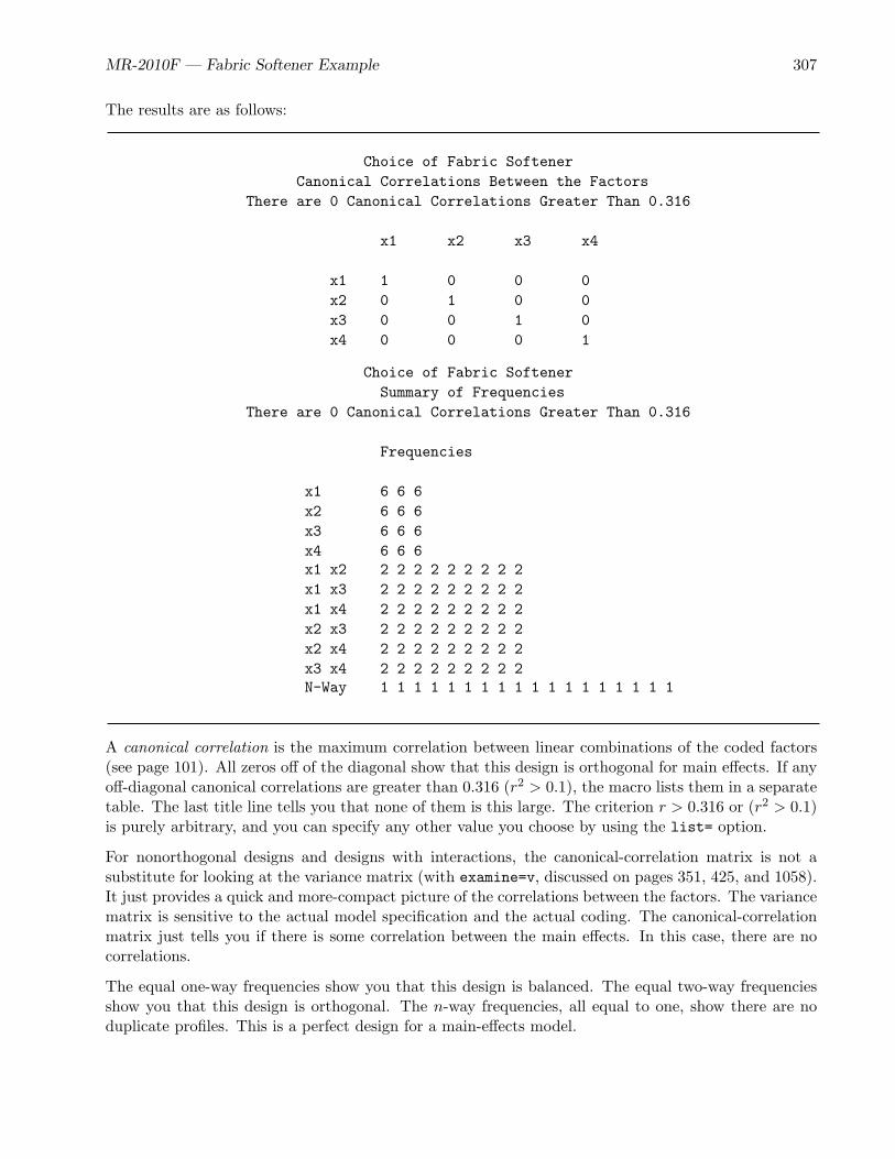
The results are as follows:
Choice of Fabric SoftenerCanonical Correlations Between the Factors
There are 0 Canonical Correlations Greater Than 0.316
x1 x2 x3 x4
x1 1 0 0 0x2 0 1 0 0x3 0 0 1 0x4 0 0 0 1
Choice of Fabric SoftenerSummary of Frequencies
There are 0 Canonical Correlations Greater Than 0.316
Frequencies
x1 6 6 6x2 6 6 6x3 6 6 6x4 6 6 6x1 x2 2 2 2 2 2 2 2 2 2x1 x3 2 2 2 2 2 2 2 2 2x1 x4 2 2 2 2 2 2 2 2 2x2 x3 2 2 2 2 2 2 2 2 2x2 x4 2 2 2 2 2 2 2 2 2x3 x4 2 2 2 2 2 2 2 2 2N-Way 1 1 1 1 1 1 1 1 1 1 1 1 1 1 1 1 1 1
A canonical correlation is the maximum correlation between linear combinations of the coded factors(see page 101). All zeros off of the diagonal show that this design is orthogonal for main effects. If anyoff-diagonal canonical correlations are greater than 0.316 (r2 > 0.1), the macro lists them in a separatetable. The last title line tells you that none of them is this large. The criterion r > 0.316 or (r2 > 0.1)is purely arbitrary, and you can specify any other value you choose by using the list= option.
For nonorthogonal designs and designs with interactions, the canonical-correlation matrix is not asubstitute for looking at the variance matrix (with examine=v, discussed on pages 351, 425, and 1058).It just provides a quick and more-compact picture of the correlations between the factors. The variancematrix is sensitive to the actual model specification and the actual coding. The canonical-correlationmatrix just tells you if there is some correlation between the main effects. In this case, there are nocorrelations.
The equal one-way frequencies show you that this design is balanced. The equal two-way frequenciesshow you that this design is orthogonal. The n-way frequencies, all equal to one, show there are noduplicate profiles. This is a perfect design for a main-effects model.

308 MR-2010F — Discrete Choice
You should always check the n-way frequencies to ensure that you do not have duplicates. For thissituation for example, a 100% D-efficient design exists where each run appears twice. It consists of twocopies of the fractional-factorial design 34 in 9 runs. When you get duplicates, specify options=nodupsin the %MktEx macro, or sometimes you can just change the random number seed. Most designs donot have duplicates, so it is better to specify options=nodups only after you have found a design withduplicates. The no-duplicates constraint greatly slows down the algorithm.
The %MktEval macro produces a very compact summary of the design, hence some information, forexample, the levels to which the frequencies correspond, is not shown. You can use the print=freqsoption to get a less compact and more detailed display as follows:
%mkteval(data=design, print=freqs)
Portions of the results are as follows:
Choice of Fabric SoftenerFrequencies
Effects Frequency x1 x2 x3 x4
x1 6 1 . . .6 2 . . .6 3 . . .
x2 6 . 1 . .6 . 2 . .6 . 3 . .
.
.
.
x1 x2 2 1 1 . .2 1 2 . .2 1 3 . .2 2 1 . .2 2 2 . .2 2 3 . .2 3 1 . .2 3 2 . .2 3 3 . .
.
.
.

MR-2010F — Fabric Softener Example 309
x3 x4 2 . . 1 12 . . 1 22 . . 1 32 . . 2 12 . . 2 22 . . 2 32 . . 3 12 . . 3 22 . . 3 3
N-Way 1 1 1 1 11 1 1 2 21 1 2 1 31 1 2 3 11 1 3 2 31 1 3 3 21 2 1 1 31 2 1 3 11 2 2 2 21 2 2 3 31 2 3 1 21 2 3 2 11 3 1 2 31 3 1 3 21 3 2 1 21 3 2 2 11 3 3 1 11 3 3 3 3
The Randomized Design and Postprocessing
The design we just looked at and examined is in the default output data set, Design. The Designdata set is the last data set created by the %MktEx macro, so it is the data set that you see if you runPROC PRINT or the %MktEval macro without specifying the data= option. The Design data set issorted, and often the first row consists entirely of ones. For these reasons, you should actually use therandomized design. In the randomized design, the choice sets are presented in a random order andthe levels have been randomly reassigned. Neither of these operations affects the design D-efficiency,balance, or orthogonality, so the %MktEval results from the Design data set are valid, even if youultimately use the Randomized data set. The macro automatically randomizes the design and storesthe results in a data set called Randomized. The next steps assign formats and labels and store theresults in a SAS data set sasuser.SoftenerLinDes. It is important to store the design in a permanentSAS data set or in some other permanent form so that it is available for analysis after the data arecollected.
Every SAS data set has a two-level name of the form libref.filename. You can always referencea file with its two-level name. However, you can also use a one-level name, and then that data setis stored in temporary SAS data library with a libref of Work. Temporary data sets are deleted at

310 MR-2010F — Discrete Choice
the end of your SAS session, so any data that must be saved needs to be stored in a permanent SASdata set. The libref called sasuser is automatically available for permanent storage in most SASinstallations. Furthermore, you can make your own libref using a libname statement. You mightwish to create a separate library for each project. The latter approach of using a libname statement isusually preferable, but for our purposes, mainly to avoid discussing issues of host-specific paths and filenames, we use sasuser. See your BASE SAS documentation and SAS Companion for your operatingsystem for more information about data libraries, libref, and libname. The following step creates apermanent SAS data set:
data sasuser.SoftenerLinDes;set randomized;format x1-x&mm1 price.;label x1 = ’Sploosh’ x2 = ’Plumbbob’ x3 = ’Platter’ x4 = ’Moosey’;run;
The following step displays the final design:
proc print data=sasuser.SoftenerLinDes label; /* print final design */title2 ’Efficient Design’;run;
The results are as follows:
Choice of Fabric SoftenerEfficient Design
Obs Sploosh Plumbbob Platter Moosey
1 $1.99 $1.99 $1.99 $2.492 $2.49 $1.49 $1.49 $1.993 $1.49 $2.49 $2.49 $1.494 $2.49 $1.99 $2.49 $1.995 $1.49 $1.49 $1.49 $2.496 $1.49 $2.49 $1.99 $1.99
7 $2.49 $1.99 $1.99 $1.498 $2.49 $2.49 $1.49 $1.499 $1.99 $1.49 $2.49 $1.4910 $1.49 $1.49 $1.99 $1.4911 $1.99 $2.49 $1.49 $2.4912 $1.49 $1.99 $1.49 $1.99
13 $1.99 $1.99 $1.49 $1.4914 $1.49 $1.99 $2.49 $2.4915 $2.49 $1.49 $2.49 $2.4916 $1.99 $2.49 $2.49 $1.9917 $1.99 $1.49 $1.99 $1.9918 $2.49 $2.49 $1.99 $2.49

MR-2010F — Fabric Softener Example 311
From the Linear Arrangement to a Choice Design
The randomized design is now in a useful form for making the questionnaire, which is discussed in thenext section. However, it is not in the final choice-design form that is needed for analysis and for thelast evaluation that we should perform before collecting data. In this section, we convert our lineararrangement to a choice design and evaluate its goodness for a choice model.
Our linear arrangement, which we stored in a permanent SAS data set, sasuser.SoftenerLinDes, isarranged with one row per choice set. For analysis, we need a choice design with one row for eachalternative of each choice set. We call the randomized design a linear arrangement (see page 67) becausewe used the %MktEx macro to create it optimizing D-efficiency for a linear model. We use the macro%MktRoll to “roll out” the linear arrangement into the choice design, which is in the proper form foranalysis. First, we must create a data set that describes how the design is processed. We call this dataset the design key.
In this example, we want a choice design with two factors, Brand and Price. Brand has levels Sploosh,Plumbbob, Platter, Moosey, and Another. Price has levels $1.49, $1.99, and $2.49. Brand and Priceare created by different processes. The Price attribute is constructed from the factors of the lineararrangement matrix. In contrast, there is no Brand factor in the linear arrangement. Each brandis a bin into which its factors are collected. The variable Brand is named in the alt= option of the%MktRoll macro as the alternative variable, so its values are read directly out of the Key data set.Price is not named in the alt= macro option, so its values in the Key data set are variable namesfrom the linear arrangement data set. The values of Price in the final choice design are read fromthe named variables in the linear arrangement data set. The Price attribute in the choice design iscreated from the four linear arrangement factors (x1 for Sploosh, x2 for Plumbbob, x3 for Platter, x4for Moosey, and no attribute for Another, the constant alternative). The Key data set is created in thenext step. The Brand factor levels and the Price linear arrangement factors are stored in the Key dataset as follows:
title2 ’Key Data Set’;
data key;input Brand $ Price $;datalines;
Sploosh x1Plumbbob x2Platter x3Moosey x4Another .;
proc print; run;

312 MR-2010F — Discrete Choice
The results are as follows:
Choice of Fabric SoftenerKey Data Set
Obs Brand Price
1 Sploosh x12 Plumbbob x23 Platter x34 Moosey x45 Another
Note that the value of Price for alternative Another in the Key data set is blank (character missing).The period in the in-stream data set is simply a place holder, used with list input to read both characterand numeric missing data. A period is not stored with the data. Next, we use the %MktRoll macro toprocess the design as follows:
%mktroll(design=sasuser.SoftenerLinDes, key=key, alt=brand,out=sasuser.SoftenerChDes)
The %MktRoll step processes the design=sasuser.SoftenerLinDes linear arrangement data set usingthe rules specified in the key=key data set, naming the alt=brand variable as the alternative namevariable, and creating an output SAS data set called out=sasuser.SoftenerChDes, which containsthe choice design. The input design=sasuser.SoftenerLinDes data set has 18 observations, one perchoice set, and the output out=sasuser.SoftenerChDes data set has 5 × 18 = 90 observations, onefor each alternative of each choice set. The following step displays the first three observations of thelinear arrangement data set:
title2 ’Linear Arrangement (First 3 Sets)’;
proc print data=sasuser.SoftenerLinDes(obs=3); run;
The results are as follows:
Choice of Fabric SoftenerLinear Arrangement (First 3 Sets)
Obs x1 x2 x3 x4
1 $1.99 $1.99 $1.99 $2.492 $2.49 $1.49 $1.49 $1.993 $1.49 $2.49 $2.49 $1.49
These observations define the first three choice sets.
MR-2010F — Fabric Softener Example 313
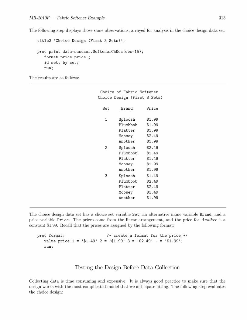
The following step displays those same observations, arrayed for analysis in the choice design data set:
title2 ’Choice Design (First 3 Sets)’;
proc print data=sasuser.SoftenerChDes(obs=15);format price price.;id set; by set;run;
The results are as follows:
Choice of Fabric SoftenerChoice Design (First 3 Sets)
Set Brand Price
1 Sploosh $1.99Plumbbob $1.99Platter $1.99Moosey $2.49Another $1.99
2 Sploosh $2.49Plumbbob $1.49Platter $1.49Moosey $1.99Another $1.99
3 Sploosh $1.49Plumbbob $2.49Platter $2.49Moosey $1.49Another $1.99
The choice design data set has a choice set variable Set, an alternative name variable Brand, and aprice variable Price. The prices come from the linear arrangement, and the price for Another is aconstant $1.99. Recall that the prices are assigned by the following format:
proc format; /* create a format for the price */value price 1 = ’$1.49’ 2 = ’$1.99’ 3 = ’$2.49’ . = ’$1.99’;run;
Testing the Design Before Data Collection
Collecting data is time consuming and expensive. It is always good practice to make sure that thedesign works with the most complicated model that we anticipate fitting. The following step evaluatesthe choice design:

314 MR-2010F — Discrete Choice
title2 ’Evaluate the Choice Design’;
%choiceff(data=sasuser.SoftenerChDes,/* candidate set of choice sets */init=sasuser.SoftenerChDes(keep=set), /* select these sets */intiter=0, /* evaluate without internal iterations */
/* main effects with ref cell coding *//* ref level for brand is ’Another’ *//* ref level for price is $1.99 */
model=class(brand price / zero=’Another’ ’$1.99’) /lprefix=0 /* lpr=0 labels created from just levels*/cprefix=0%str(;) /* cpr=0 names created from just levels */format price price.,/* trick: format passed in with model */
nsets=&n, /* number of choice sets */nalts=&m, /* number of alternatives */beta=zero) /* assumed beta vector, Ho: b=0 */
The %ChoicEff macro has two uses. You can use it to search for an efficient choice design, or you canuse it to evaluate a choice design including designs that are generated using other methods such as the%MktEx and %MktRoll macros. It is this latter use that is illustrated here.
The way you check a design like this is to first name it in the data= option. This is the candidate setthat contains all of the choice sets that we will consider. In addition, the same design is named in theinit= option. The full specification is init=sasuser.SoftenerChDes(keep=set). Just the variableSet is kept. It is used to bring in just the indicated choice sets from the data= design, which in thiscase is all of them. The option nsets=&n specifies that there are &n=18 choice sets, and nalts=&mspecifies that there are &m=5 alternatives. The option beta=zero specifies that we are assuming fordesign evaluation purposes the null hypothesis that all of the betas or part-worth utilities are zero.You can evaluate the design for other parameter vectors by specifying a list of numbers after beta=.This will change the variances and standard errors. We also specify intiter=0 which specifies zerointernal iterations. We use zero internal iterations when we want to evaluate an initial design, but notattempt to improve it. The model= option option specifies the model.
The model specification contains everything that appears in the TRANSREG procedure’s modelstatement for coding the design. The specification class(brand price / zero=’Another’ ’$1.99’)names the brand and price variable as a classification variables and asks for coded variables for everylevel except ’Another’ for brand and ’$1.99’ for price. The levels ’Another’ and ’$1.99’ are thereference levels for the two attributes. In a p-level factor, there are at most p− 1 nonzero parameters.
The lprefix=0 option specifies that when labels are created for the binary variables, zero characters ofthe original variable name should be used as a prefix. This means that the labels are created only fromthe level values. For example, ’Sploosh’ and ’Plumbbob’ are created as labels not ’Brand Sploosh’and ’Brand Plumbbob’. The cprefix=0 option specifies that when names are created for the binaryvariables, zero characters of the original variable name should be used as a prefix. This means that thenames are created only from the level values. The c in cprefix stands for class.
The code following the cprefix= specification is a bit of a trick. The %ChoicEff macro generates amodel statement for PROC TRANSREG using the specified value like this:
model &model;
MR-2010F — Fabric Softener Example 315
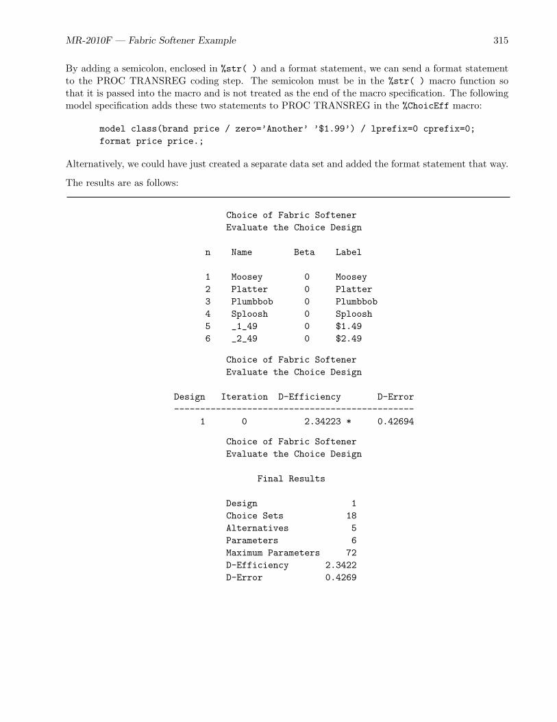
By adding a semicolon, enclosed in %str( ) and a format statement, we can send a format statementto the PROC TRANSREG coding step. The semicolon must be in the %str( ) macro function sothat it is passed into the macro and is not treated as the end of the macro specification. The followingmodel specification adds these two statements to PROC TRANSREG in the %ChoicEff macro:
model class(brand price / zero=’Another’ ’$1.99’) / lprefix=0 cprefix=0;format price price.;
Alternatively, we could have just created a separate data set and added the format statement that way.
The results are as follows:
Choice of Fabric SoftenerEvaluate the Choice Design
n Name Beta Label
1 Moosey 0 Moosey2 Platter 0 Platter3 Plumbbob 0 Plumbbob4 Sploosh 0 Sploosh5 _1_49 0 $1.496 _2_49 0 $2.49
Choice of Fabric SoftenerEvaluate the Choice Design
Design Iteration D-Efficiency D-Error----------------------------------------------
1 0 2.34223 * 0.42694
Choice of Fabric SoftenerEvaluate the Choice Design
Final Results
Design 1Choice Sets 18Alternatives 5Parameters 6Maximum Parameters 72D-Efficiency 2.3422D-Error 0.4269
316 MR-2010F — Discrete Choice
Choice of Fabric SoftenerEvaluate the Choice Design
Variable Standardn Name Label Variance DF Error
1 Moosey Moosey 0.72917 1 0.853912 Platter Platter 0.72917 1 0.853913 Plumbbob Plumbbob 0.72917 1 0.853914 Sploosh Sploosh 0.72917 1 0.853915 _1_49 $1.49 0.52083 1 0.721696 _2_49 $2.49 0.52083 1 0.72169
==6
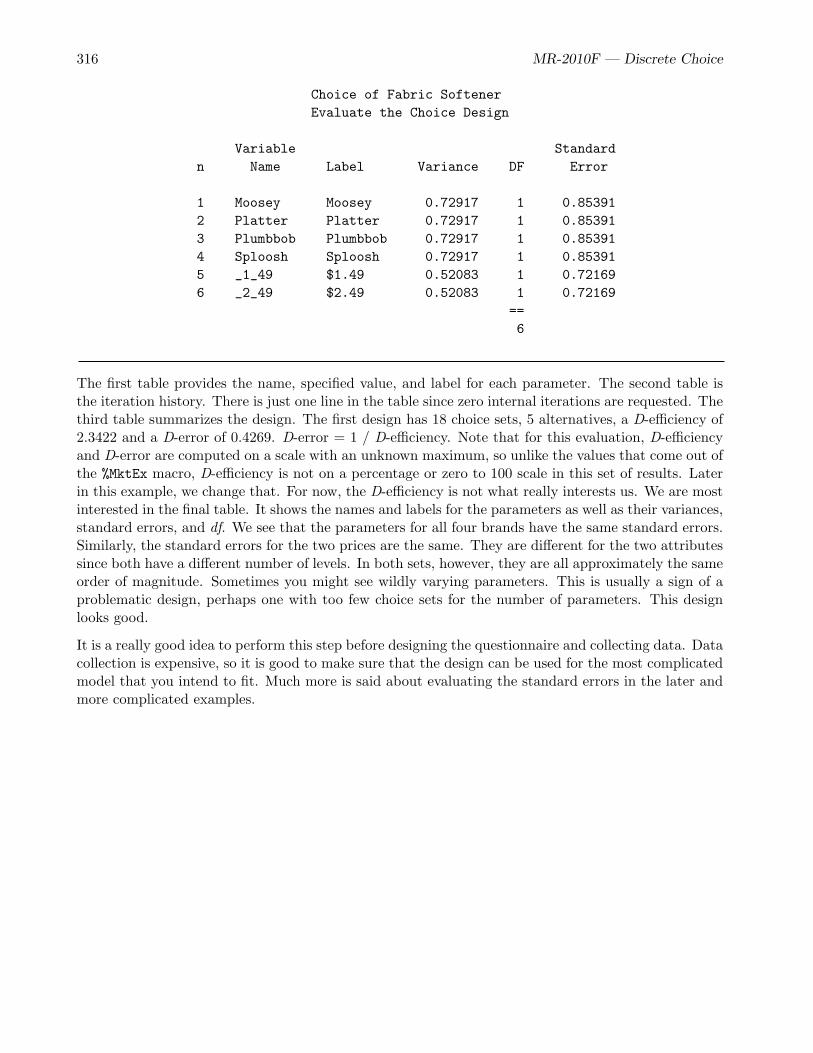
The first table provides the name, specified value, and label for each parameter. The second table isthe iteration history. There is just one line in the table since zero internal iterations are requested. Thethird table summarizes the design. The first design has 18 choice sets, 5 alternatives, a D-efficiency of2.3422 and a D-error of 0.4269. D-error = 1 / D-efficiency. Note that for this evaluation, D-efficiencyand D-error are computed on a scale with an unknown maximum, so unlike the values that come out ofthe %MktEx macro, D-efficiency is not on a percentage or zero to 100 scale in this set of results. Laterin this example, we change that. For now, the D-efficiency is not what really interests us. We are mostinterested in the final table. It shows the names and labels for the parameters as well as their variances,standard errors, and df. We see that the parameters for all four brands have the same standard errors.Similarly, the standard errors for the two prices are the same. They are different for the two attributessince both have a different number of levels. In both sets, however, they are all approximately the sameorder of magnitude. Sometimes you might see wildly varying parameters. This is usually a sign of aproblematic design, perhaps one with too few choice sets for the number of parameters. This designlooks good.
It is a really good idea to perform this step before designing the questionnaire and collecting data. Datacollection is expensive, so it is good to make sure that the design can be used for the most complicatedmodel that you intend to fit. Much more is said about evaluating the standard errors in the later andmore complicated examples.
MR-2010F — Fabric Softener Example 317
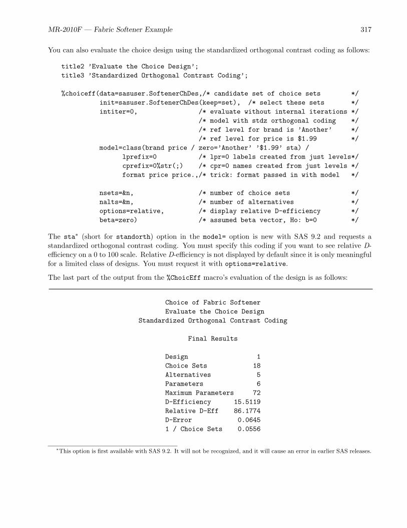
You can also evaluate the choice design using the standardized orthogonal contrast coding as follows:
title2 ’Evaluate the Choice Design’;title3 ’Standardized Orthogonal Contrast Coding’;
%choiceff(data=sasuser.SoftenerChDes,/* candidate set of choice sets */init=sasuser.SoftenerChDes(keep=set), /* select these sets */intiter=0, /* evaluate without internal iterations */
/* model with stdz orthogonal coding *//* ref level for brand is ’Another’ *//* ref level for price is $1.99 */
model=class(brand price / zero=’Another’ ’$1.99’ sta) /lprefix=0 /* lpr=0 labels created from just levels*/cprefix=0%str(;) /* cpr=0 names created from just levels */format price price.,/* trick: format passed in with model */
nsets=&n, /* number of choice sets */nalts=&m, /* number of alternatives */options=relative, /* display relative D-efficiency */beta=zero) /* assumed beta vector, Ho: b=0 */
The sta∗ (short for standorth) option in the model= option is new with SAS 9.2 and requests astandardized orthogonal contrast coding. You must specify this coding if you want to see relative D-efficiency on a 0 to 100 scale. Relative D-efficiency is not displayed by default since it is only meaningfulfor a limited class of designs. You must request it with options=relative.
The last part of the output from the %ChoicEff macro’s evaluation of the design is as follows:
Choice of Fabric SoftenerEvaluate the Choice Design
Standardized Orthogonal Contrast Coding
Final Results
Design 1Choice Sets 18Alternatives 5Parameters 6Maximum Parameters 72D-Efficiency 15.5119Relative D-Eff 86.1774D-Error 0.06451 / Choice Sets 0.0556
∗This option is first available with SAS 9.2. It will not be recognized, and it will cause an error in earlier SAS releases.

318 MR-2010F — Discrete Choice
Choice of Fabric Softener 9Evaluate the Choice Design
Standardized Orthogonal Contrast Coding
Variable Standardn Name Label Variance DF Error
1 Moosey Moosey 0.055556 1 0.235702 Platter Platter 0.055556 1 0.235703 Plumbbob Plumbbob 0.055556 1 0.235704 Sploosh Sploosh 0.055556 1 0.235705 _1_49 $1.49 0.086806 1 0.294636 _2_49 $2.49 0.086806 1 0.29463
==6
In the first table, we see D-efficiency equals 15.5119 (as opposed to 2.3422 previous). D-error is alwaysequal to 1 / D-efficiency. If this were a perfect choice design like we can achieve for some genericdesigns, then D-efficiency would equal 18, and the number of choice sets and D-error and all of thevariances would equal one over the number of choice sets (0.0556). Relative D-efficiency equals 100times D-efficiency divided by the number of choice sets. It is 100 for perfect designs. In this case,relative D-efficiency = 86.1774, and all of the variances for the price parameters are larger than 0.556.Note the relative D-efficiency = 86.1774 provides a pessimistic view of the goodness of this design. Thisvalue is computed relative to the value you would get for an unrestricted design (one that does nothave a constant alternative). 100% relative D-efficiency is not possible with a constant alternative andusing the number of choice sets as a base line since all alternatives must vary optimally to achieve 100%efficiency. Furthermore, this design has five alternatives. There are five brands, one for each alternative,which is ideal. Hence, the variances for the brand parameters are at the minimum. However, there areonly three prices. Since 3 does not evenly divide the 5 alternatives, there is no way we can achieve 100%efficiency by scaling D-efficiency relative to the number of choice sets. Hence, the variances for theprice parameters are greater than their minimum. This design looks reasonable because the variancesare not too far removed from one over the number of choice sets.
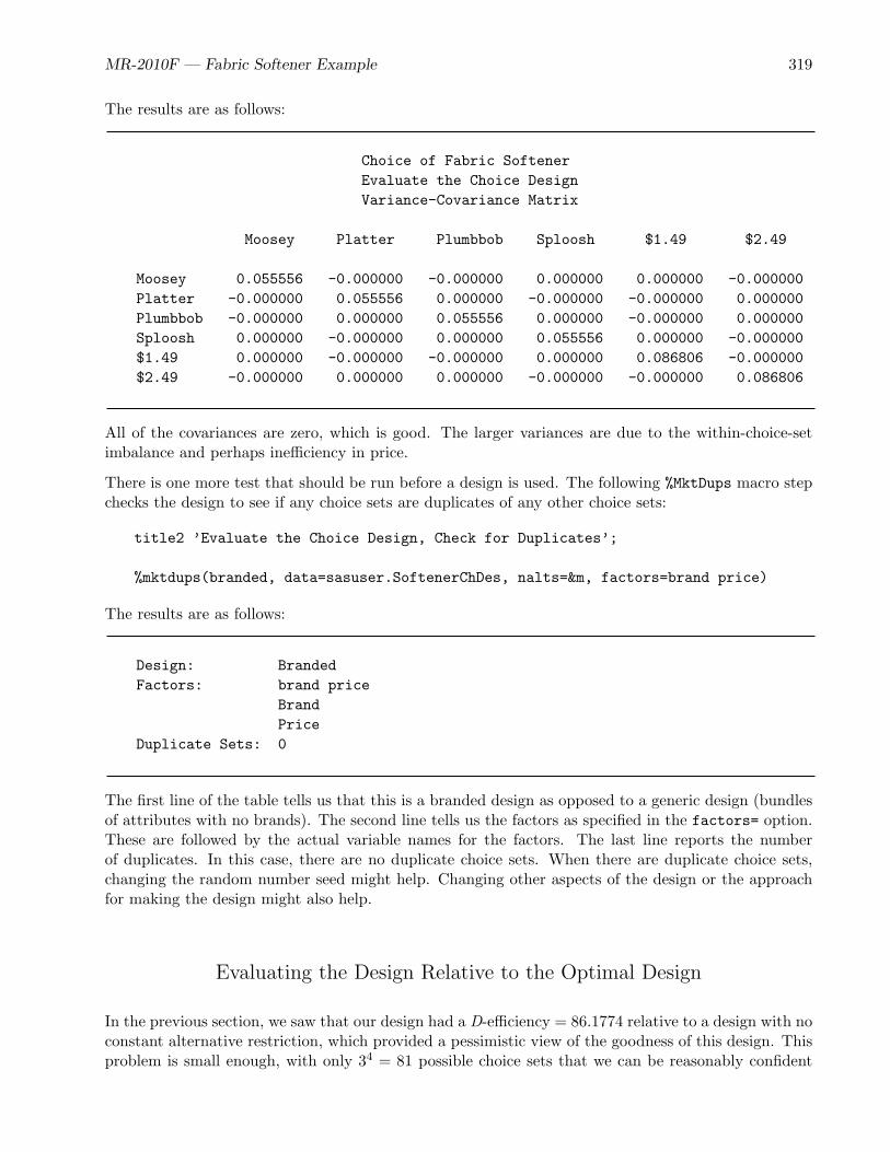
The %ChoicEff macro displays the variances. You can display the full matrix of variances and covari-ances, which the %ChoicEff macro stores in a SAS data set, as follows:
proc print data=bestcov label;title3 ’Variance-Covariance Matrix’;id __label;label __label = ’00’x;var Moosey -- _2_49;run;
MR-2010F — Fabric Softener Example 319
The results are as follows:
Choice of Fabric SoftenerEvaluate the Choice DesignVariance-Covariance Matrix
Moosey Platter Plumbbob Sploosh $1.49 $2.49
Moosey 0.055556 -0.000000 -0.000000 0.000000 0.000000 -0.000000Platter -0.000000 0.055556 0.000000 -0.000000 -0.000000 0.000000Plumbbob -0.000000 0.000000 0.055556 0.000000 -0.000000 0.000000Sploosh 0.000000 -0.000000 0.000000 0.055556 0.000000 -0.000000$1.49 0.000000 -0.000000 -0.000000 0.000000 0.086806 -0.000000$2.49 -0.000000 0.000000 0.000000 -0.000000 -0.000000 0.086806
All of the covariances are zero, which is good. The larger variances are due to the within-choice-setimbalance and perhaps inefficiency in price.
There is one more test that should be run before a design is used. The following %MktDups macro stepchecks the design to see if any choice sets are duplicates of any other choice sets:
title2 ’Evaluate the Choice Design, Check for Duplicates’;
%mktdups(branded, data=sasuser.SoftenerChDes, nalts=&m, factors=brand price)
The results are as follows:
Design: BrandedFactors: brand price
BrandPrice
Duplicate Sets: 0
The first line of the table tells us that this is a branded design as opposed to a generic design (bundlesof attributes with no brands). The second line tells us the factors as specified in the factors= option.These are followed by the actual variable names for the factors. The last line reports the numberof duplicates. In this case, there are no duplicate choice sets. When there are duplicate choice sets,changing the random number seed might help. Changing other aspects of the design or the approachfor making the design might also help.
Evaluating the Design Relative to the Optimal Design
In the previous section, we saw that our design had a D-efficiency = 86.1774 relative to a design with noconstant alternative restriction, which provided a pessimistic view of the goodness of this design. Thisproblem is small enough, with only 34 = 81 possible choice sets that we can be reasonably confident

320 MR-2010F — Discrete Choice
that the %ChoicEff macro will find the optimal design given a candidate set of all possible choice sets.We can then use the D-efficiency of the optimal design in the relative D-efficiency computations forour design to measure the goodness of our design for this particular model. This is illustrated in thissection. It proceeds very similarly to the steps shown previously, only this time, rather than giving the%ChoicEff macro a set of choice sets to evaluate, it is given a set of candidate choice sets from whichto construct a design. The following steps create a candidate set of all possible choice sets:
%mktex(3 ** 4, n=81)
data TestLinDes;set design;format x1-x&mm1 price.;label x1 = ’Sploosh’ x2 = ’Plumbbob’ x3 = ’Platter’ x4 = ’Moosey’;run;
data key;input Brand $ Price $;datalines;
Sploosh x1Plumbbob x2Platter x3Moosey x4Another .;
%mktroll(design=TestLinDes, key=key, alt=brand, out=TestChDes)
The following step searches for an optimal design:
%choiceff(data=TestChDes, /* candidate set of choice sets *//* model with stdz orthogonal coding *//* ref level for brand is ’Another’ *//* ref level for price is $1.99 */
model=class(brand price / zero=’Another’ ’$1.99’ sta) /lprefix=0 /* lpr=0 labels created from just levels*/cprefix=0%str(;) /* cpr=0 names created from just levels */format price price.,/* trick: format passed in with model */
seed=205, /* random number seed */maxiter=50, /* maximum number of designs to make */nsets=&n, /* number of choice sets */nalts=&m, /* number of alternatives */options=relative, /* display relative D-efficiency */beta=zero) /* assumed beta vector, Ho: b=0 */

MR-2010F — Fabric Softener Example 321
Some of the results are as follows:
Choice of Fabric SoftenerEvaluate the Choice Design, Check for Duplicates
Final Results
Design 1Choice Sets 18Alternatives 5Parameters 6Maximum Parameters 72D-Efficiency 16.4264Relative D-Eff 91.2581D-Error 0.06091 / Choice Sets 0.0556
Choice of Fabric SoftenerEvaluate the Choice Design, Check for Duplicates
Variable Standardn Name Label Variance DF Error
1 Moosey Moosey 0.055556 1 0.235702 Platter Platter 0.055556 1 0.235703 Plumbbob Plumbbob 0.055556 1 0.235704 Sploosh Sploosh 0.055556 1 0.235705 _1_49 $1.49 0.073099 1 0.270376 _2_49 $2.49 0.073099 1 0.27037
==6
The iteration histories for the 50 designs that were created (not shown) all have the same D-efficiency= 16.4264. With small problems like this one, this is a good sign that the optimal design was found.
322 MR-2010F — Discrete Choice
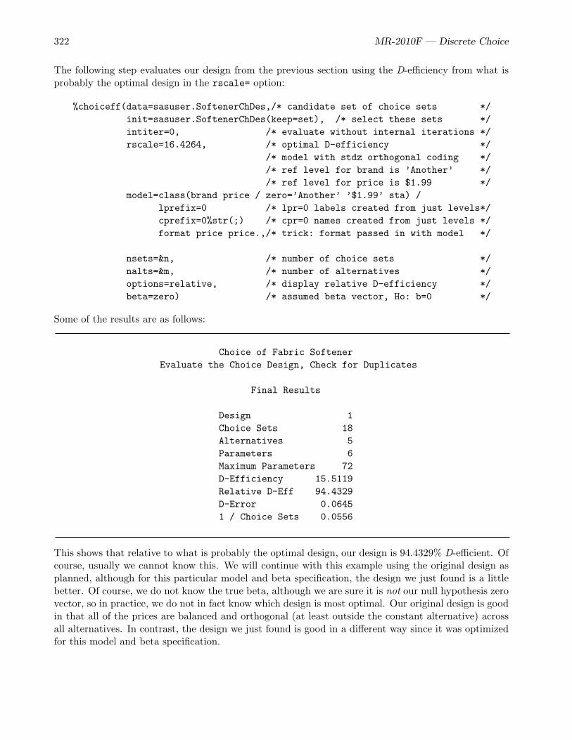
The following step evaluates our design from the previous section using the D-efficiency from what isprobably the optimal design in the rscale= option:
%choiceff(data=sasuser.SoftenerChDes,/* candidate set of choice sets */init=sasuser.SoftenerChDes(keep=set), /* select these sets */intiter=0, /* evaluate without internal iterations */rscale=16.4264, /* optimal D-efficiency */
/* model with stdz orthogonal coding *//* ref level for brand is ’Another’ *//* ref level for price is $1.99 */
model=class(brand price / zero=’Another’ ’$1.99’ sta) /lprefix=0 /* lpr=0 labels created from just levels*/cprefix=0%str(;) /* cpr=0 names created from just levels */format price price.,/* trick: format passed in with model */
nsets=&n, /* number of choice sets */nalts=&m, /* number of alternatives */options=relative, /* display relative D-efficiency */beta=zero) /* assumed beta vector, Ho: b=0 */
Some of the results are as follows:
Choice of Fabric SoftenerEvaluate the Choice Design, Check for Duplicates
Final Results
Design 1Choice Sets 18Alternatives 5Parameters 6Maximum Parameters 72D-Efficiency 15.5119Relative D-Eff 94.4329D-Error 0.06451 / Choice Sets 0.0556
This shows that relative to what is probably the optimal design, our design is 94.4329% D-efficient. Ofcourse, usually we cannot know this. We will continue with this example using the original design asplanned, although for this particular model and beta specification, the design we just found is a littlebetter. Of course, we do not know the true beta, although we are sure it is not our null hypothesis zerovector, so in practice, we do not in fact know which design is most optimal. Our original design is goodin that all of the prices are balanced and orthogonal (at least outside the constant alternative) acrossall alternatives. In contrast, the design we just found is good in a different way since it was optimizedfor this model and beta specification.

MR-2010F — Fabric Softener Example 323
Generating the Questionnaire
A questionnaire based on the design is produced using the following DATA step:
title;
data _null_; /* print questionnaire */array brands[&m] $ _temporary_ (’Sploosh’ ’Plumbbob’ ’Platter’
’Moosey’ ’Another’);array x[&m] x1-x&m;file print linesleft=ll;set sasuser.SoftenerLinDes;
x&m = 2; /* constant alternative */format x&m price.;
if _n_ = 1 or ll < 12 then do;put _page_;put @60 ’Subject: _________’ //;end;
put _n_ 2. ’) Circle your choice of ’’one of the following fabric softeners:’ /;
do brnds = 1 to &m;put ’ ’ brnds 1. ’) ’ brands[brnds] ’brand at ’
x[brnds] +(-1) ’.’ /;end;
run;
The following statement creates a constant array:
array brands[&m] $ _temporary_ (’Sploosh’ ’Plumbbob’ ’Platter’’Moosey’ ’Another’)
The array reference brands[1] accesses the string ’Sploosh’, brands[2] accesses the string ’Plumbbob’,and so on. The temporary specification means that no output data set variables are created for thisarray. The linesleft= specification in the file statement creates the variable ll, which contains thenumber of lines left on a page. This ensures that each choice set is not split over two pages.

324 MR-2010F — Discrete Choice
In the interest of space, only the first two choice sets are shown as follows:
Subject: _________
1) Circle your choice of one of the following fabric softeners:
1) Sploosh brand at $1.99.
2) Plumbbob brand at $1.99.
3) Platter brand at $1.99.
4) Moosey brand at $2.49.
5) Another brand at $1.99.
2) Circle your choice of one of the following fabric softeners:
1) Sploosh brand at $2.49.
2) Plumbbob brand at $1.49.
3) Platter brand at $1.49.
4) Moosey brand at $1.99.
5) Another brand at $1.99.
The questionnaire is printed, copied, and the data are collected.
In practice, data collection is typically much more elaborate than this. It might involve art work orphotographs, and the choice sets might be presented and the data might be collected through personalinterview or over the Web. However the choice sets are presented and the data are collected, theessential elements remain the same. Subjects are shown a set of alternatives and are asked to make achoice, then they go on to the next set.
Entering the Data
The data consist of a subject number followed by 18 integers in the range 1 to 5. These are thealternatives that are chosen for each choice set. For example, the first subject chose alternative 3(Platter brand at $1.99) in the first choice set, alternative 3 (Platter brand at $1.49) in the secondchoice set, and so on. In the interest of space, data from three subjects appear on one line. The dataare read in the following step:
MR-2010F — Fabric Softener Example 325
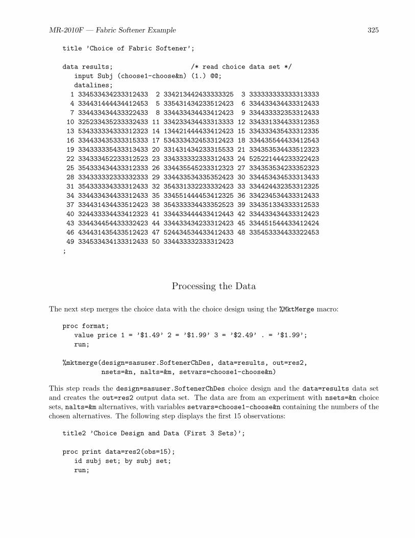
title ’Choice of Fabric Softener’;
data results; /* read choice data set */input Subj (choose1-choose&n) (1.) @@;datalines;
1 334533434233312433 2 334213442433333325 3 3333333333333133334 334431444434412453 5 335431434233512423 6 3344334344333124337 334433434433322433 8 334433434433412423 9 33443333235331243310 325233435233332433 11 334233434433313333 12 33433133443331235313 534333334333312323 14 134421444433412423 15 33433343543331233516 334433435333315333 17 534333432453312423 18 33443554443341254319 334333335433313433 20 331431434233315533 21 33435353443351232322 334333452233312523 23 334333332333312433 24 52522144423332242325 354333434433312333 26 334435545233312323 27 33435353423335232328 334333332333332333 29 334433534335352423 30 33445343453331343331 354333334333312433 32 354331332233332423 33 33442443235331232534 334433434433312433 35 334551444453412325 36 33423453443331243337 334431434433512423 38 354333334433352523 39 33435133433331253340 324433334433412323 41 334433444433412443 42 33443343443331242343 334434454433332423 44 334433434233312423 45 33445154443341242446 434431435433512423 47 524434534433412433 48 33545333443332245349 334533434133312433 50 334433332333312423;
Processing the Data
The next step merges the choice data with the choice design using the %MktMerge macro:
proc format;value price 1 = ’$1.49’ 2 = ’$1.99’ 3 = ’$2.49’ . = ’$1.99’;run;
%mktmerge(design=sasuser.SoftenerChDes, data=results, out=res2,nsets=&n, nalts=&m, setvars=choose1-choose&n)
This step reads the design=sasuser.SoftenerChDes choice design and the data=results data setand creates the out=res2 output data set. The data are from an experiment with nsets=&n choicesets, nalts=&m alternatives, with variables setvars=choose1-choose&n containing the numbers of thechosen alternatives. The following step displays the first 15 observations:
title2 ’Choice Design and Data (First 3 Sets)’;
proc print data=res2(obs=15);id subj set; by subj set;run;

326 MR-2010F — Discrete Choice
The results are as follows:
Choice of Fabric SoftenerChoice Design and Data (First 3 Sets)
Subj Set Brand Price c
1 1 Sploosh 2 2Plumbbob 2 2Platter 2 1Moosey 3 2Another . 2
1 2 Sploosh 3 2Plumbbob 1 2Platter 1 1Moosey 2 2Another . 2
1 3 Sploosh 1 2Plumbbob 3 2Platter 3 2Moosey 1 1Another . 2
The data set contains the subject ID variable Subj from the data=results data set, the Set, Brand,and Price variables from the design=sasuser.SoftenerChDes data set, and the variable c, whichindicates which alternative is chosen. The variable c contains: 1 for first choice and 2 for second orsubsequent choice. This subject chose the third alternative, Platter in the first choice set, Platter inthe second, and Moosey in the third. This data set has 4500 observations: 50 subjects times 18 choicesets times 5 alternatives.
Since we did not specify a format, we see in the design the raw design values for Price: 1, 2, 3 andmissing for the constant alternative. If we were going to treat Price as a categorical variable foranalysis, this would be fine. We would simply assign our price format to Price and designate it as aclass variable. However, in this analysis we are going to treat price as quantitative and use the actualprices in the analysis. Hence, we must convert our design values from 1, 2, 3, and . to 1.49, 1.99, 2.49,and 1.99. We cannot do this by simply assigning a format. Formats create character strings that aredisplayed in place of the original value. We need to convert a numeric variable from one set of numericvalues to another. We could use if and assignment statements. We could also use the %MktLab macro,which is used in later examples. However, instead we can use the put function to write the formattedvalue into a character string, then we read it back using a dollar format and the input function. Forexample, the expression put(price, price.) converts a number, say 2, into a string (in this case’$1.99’), then the input function reads the string and converts it to a numeric 1.99. The following stepalso assigns a label to the variable Price:
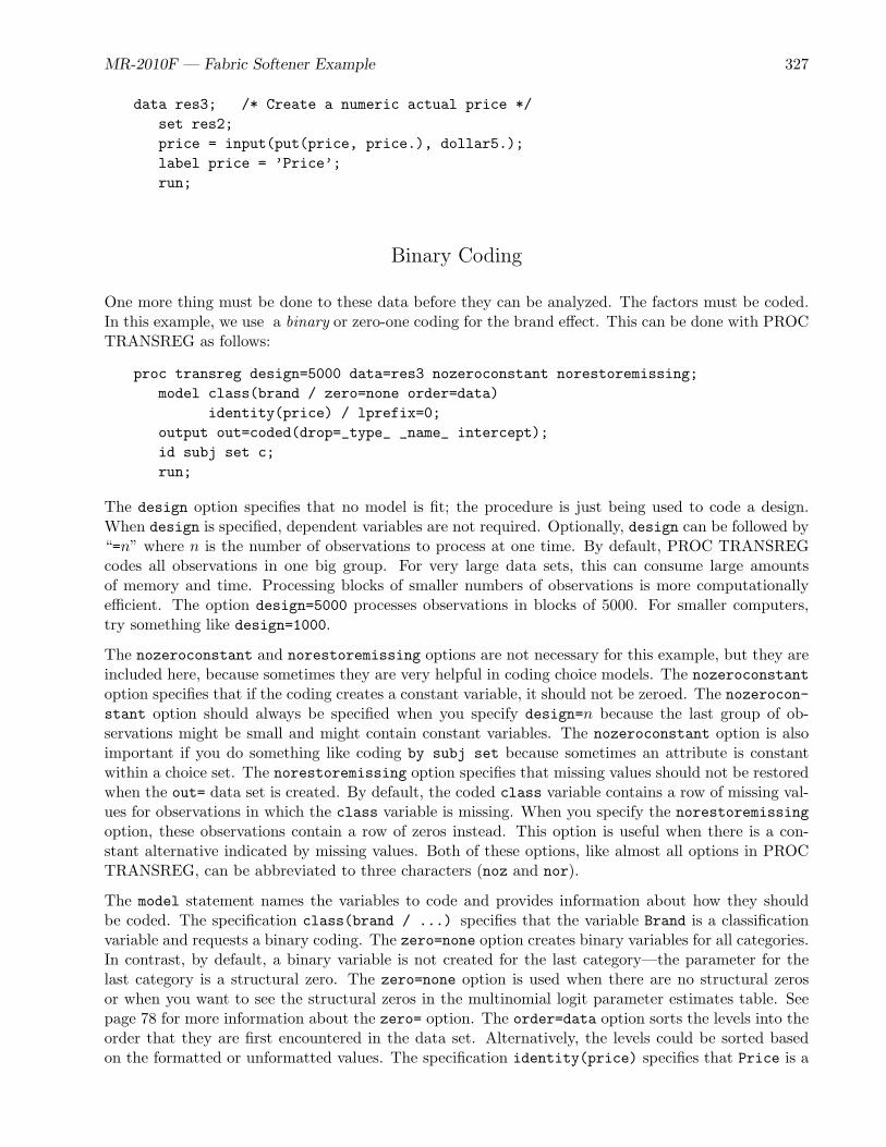
MR-2010F — Fabric Softener Example 327
data res3; /* Create a numeric actual price */set res2;price = input(put(price, price.), dollar5.);label price = ’Price’;run;
Binary Coding
One more thing must be done to these data before they can be analyzed. The factors must be coded.In this example, we use a binary or zero-one coding for the brand effect. This can be done with PROCTRANSREG as follows:
proc transreg design=5000 data=res3 nozeroconstant norestoremissing;model class(brand / zero=none order=data)
identity(price) / lprefix=0;output out=coded(drop=_type_ _name_ intercept);id subj set c;run;
The design option specifies that no model is fit; the procedure is just being used to code a design.When design is specified, dependent variables are not required. Optionally, design can be followed by“=n” where n is the number of observations to process at one time. By default, PROC TRANSREGcodes all observations in one big group. For very large data sets, this can consume large amountsof memory and time. Processing blocks of smaller numbers of observations is more computationallyefficient. The option design=5000 processes observations in blocks of 5000. For smaller computers,try something like design=1000.
The nozeroconstant and norestoremissing options are not necessary for this example, but they areincluded here, because sometimes they are very helpful in coding choice models. The nozeroconstantoption specifies that if the coding creates a constant variable, it should not be zeroed. The nozerocon-stant option should always be specified when you specify design=n because the last group of ob-servations might be small and might contain constant variables. The nozeroconstant option is alsoimportant if you do something like coding by subj set because sometimes an attribute is constantwithin a choice set. The norestoremissing option specifies that missing values should not be restoredwhen the out= data set is created. By default, the coded class variable contains a row of missing val-ues for observations in which the class variable is missing. When you specify the norestoremissingoption, these observations contain a row of zeros instead. This option is useful when there is a con-stant alternative indicated by missing values. Both of these options, like almost all options in PROCTRANSREG, can be abbreviated to three characters (noz and nor).
The model statement names the variables to code and provides information about how they shouldbe coded. The specification class(brand / ...) specifies that the variable Brand is a classificationvariable and requests a binary coding. The zero=none option creates binary variables for all categories.In contrast, by default, a binary variable is not created for the last category—the parameter for thelast category is a structural zero. The zero=none option is used when there are no structural zerosor when you want to see the structural zeros in the multinomial logit parameter estimates table. Seepage 78 for more information about the zero= option. The order=data option sorts the levels into theorder that they are first encountered in the data set. Alternatively, the levels could be sorted basedon the formatted or unformatted values. The specification identity(price) specifies that Price is a

328 MR-2010F — Discrete Choice
quantitative attribute that should be analyzed as is (not expanded into indicator variables).
The lprefix=0 option specifies that when labels are created for the binary variables, zero charactersof the original variable name should be used as a prefix.
An output statement names the output data set and drops variables that are not needed. Thesevariables do not have to be dropped. However, since they are variable names that are often found inspecial data set types, PROC PHREG displays warnings when it finds them. Dropping the variablesprevents the warnings. Finally, the id statement names the additional variables that we want copiedfrom the input to the output data set. The next steps display the first three coded choice sets:
proc print data=coded(obs=15) label;title2 ’First 15 Observations of Analysis Data Set’;id subj set c;by subj set;run;
The results are as follows:
Choice of Fabric SoftenerFirst 15 Observations of Analysis Data Set
Subj Set c Sploosh Plumbbob Platter Moosey Another Price Brand
1 1 2 1 0 0 0 0 1.99 Sploosh2 0 1 0 0 0 1.99 Plumbbob1 0 0 1 0 0 1.99 Platter2 0 0 0 1 0 2.49 Moosey2 0 0 0 0 1 1.99 Another
1 2 2 1 0 0 0 0 2.49 Sploosh2 0 1 0 0 0 1.49 Plumbbob1 0 0 1 0 0 1.49 Platter2 0 0 0 1 0 1.99 Moosey2 0 0 0 0 1 1.99 Another
1 3 2 1 0 0 0 0 1.49 Sploosh2 0 1 0 0 0 2.49 Plumbbob2 0 0 1 0 0 2.49 Platter1 0 0 0 1 0 1.49 Moosey2 0 0 0 0 1 1.99 Another
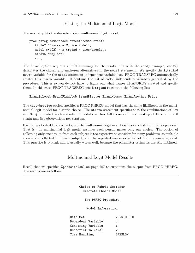
MR-2010F — Fabric Softener Example 329
Fitting the Multinomial Logit Model
The next step fits the discrete choice, multinomial logit model:
proc phreg data=coded outest=betas brief;title2 ’Discrete Choice Model’;model c*c(2) = &_trgind / ties=breslow;strata subj set;run;
The brief option requests a brief summary for the strata. As with the candy example, c*c(2)designates the chosen and unchosen alternatives in the model statement. We specify the & trgindmacro variable for the model statement independent variable list. PROC TRANSREG automaticallycreates this macro variable. It contains the list of coded independent variables generated by theprocedure. This is so you do not have to figure out what names TRANSREG created and specifythem. In this case, PROC TRANSREG sets & trgind to contain the following list:
BrandSploosh BrandPlumbbob BrandPlatter BrandMoosey BrandAnother Price
The ties=breslow option specifies a PROC PHREG model that has the same likelihood as the multi-nomial logit model for discrete choice. The strata statement specifies that the combinations of Setand Subj indicate the choice sets. This data set has 4500 observations consisting of 18 × 50 = 900strata and five observations per stratum.
Each subject rated 18 choice sets, but the multinomial logit model assumes each stratum is independent.That is, the multinomial logit model assumes each person makes only one choice. The option ofcollecting only one datum from each subject is too expensive to consider for many problems, so multiplechoices are collected from each subject, and the repeated measures aspect of the problem is ignored.This practice is typical, and it usually works well, because the parameter estimates are still unbiased.
Multinomial Logit Model Results
Recall that we specified %phchoice(on) on page 287 to customize the output from PROC PHREG.The results are as follows:
Choice of Fabric SoftenerDiscrete Choice Model
The PHREG Procedure
Model Information
Data Set WORK.CODEDDependent Variable cCensoring Variable cCensoring Value(s) 2Ties Handling BRESLOW
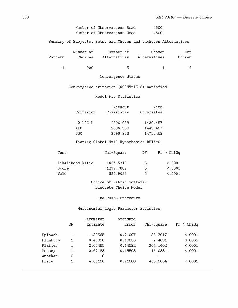
330 MR-2010F — Discrete Choice
Number of Observations Read 4500Number of Observations Used 4500
Summary of Subjects, Sets, and Chosen and Unchosen Alternatives
Number of Number of Chosen NotPattern Choices Alternatives Alternatives Chosen
1 900 5 1 4
Convergence Status
Convergence criterion (GCONV=1E-8) satisfied.
Model Fit Statistics
Without WithCriterion Covariates Covariates
-2 LOG L 2896.988 1439.457AIC 2896.988 1449.457SBC 2896.988 1473.469
Testing Global Null Hypothesis: BETA=0
Test Chi-Square DF Pr > ChiSq
Likelihood Ratio 1457.5310 5 <.0001Score 1299.7889 5 <.0001Wald 635.9093 5 <.0001
Choice of Fabric SoftenerDiscrete Choice Model
The PHREG Procedure
Multinomial Logit Parameter Estimates
Parameter StandardDF Estimate Error Chi-Square Pr > ChiSq
Sploosh 1 -1.30565 0.21097 38.3017 <.0001Plumbbob 1 -0.49090 0.18035 7.4091 0.0065Platter 1 2.08485 0.14592 204.1402 <.0001Moosey 1 0.62183 0.15503 16.0884 <.0001Another 0 0 . . .Price 1 -4.60150 0.21608 453.5054 <.0001
MR-2010F — Fabric Softener Example 331
The procedure output begins with information about the data set, variables, options, and numberof observations read. This is followed by information about the 900 strata. Since the brief optionis specified, this table contains one row for each stratum pattern. In contrast, the default table has900 rows, one for each choice set and subject combination. Each subject and choice set combinationconsists of a total of five observations, one that is chosen and four that are not chosen. This patternis observed 900 times. This table provides a check on data entry. Unless we have an availability orallocation study (page 524) or a nonconstant number of alternatives in different choice sets, we expectto see one pattern of results where one of the m alternatives is chosen for each choice set. If you donot observe this for a study like this, there is probably a mistake in the data entry or processing.
The most to least preferred brands are: Platter, Moosey, Another, Plumbbob, and Sploosh. Increases inprice have a negative utility. For example, the predicted utility of Platter brand at $1.99 is xiβ which is(0 0 1 0 0 $1.99) (−1.31 −0.49 2.08 0.62 0 −4.60)′ = 2.08 + 1.99 × −4.60 = −7.07Since Price is analyzed as a quantitative attribute, we can see for example that the utility of Platterat $1.89, which is not in any choice set, is 2.08 + 1.89×−4.60 = −6.61, which is a $0.10× 4.60 = 0.46increase in utility.
Probability of Choice
These next steps compute the expected probability that each alternative is chosen within each choice set.These steps could easily be modified to compute expected market share for hypothetical marketplacesthat do not directly correspond to the choice sets. Note, however, that a term like “expected marketshare,” while widely used, is a misnomer. Without purchase volume data, it is unlikely that thesenumbers mirror true market share.
First, PROC SCORE is used to compute the predicted utility for each alternative as follows:
proc score data=coded(where=(subj=1) drop=c)score=betas type=parms out=p;
var &_trgind;run;
The data set to be scored is named with the data= option, and the coefficients are specified in theoption score=beta. Note that we only need to read all of the choice sets once, since the parameterestimates are computed in an aggregate analysis. This is why we specified where=(subj=1). We do notneed xjβ for each of the different subjects. We dropped the variable c from the Coded data set sincethis name is used by PROC SCORE for the results (xjβ). The option type=parms specifies that thescore= data set contains the parameters in TYPE = ’PARMS’ observations. The output data set withthe predicted utilities is named P. Scoring is based on the coded variables from PROC TRANSREG,whose names are contained in the macro variable & trgind. The next step exponentiates xjβ:
data p2;set p;p = exp(c);run;

332 MR-2010F — Discrete Choice
Next, exp(xjβ) is summed for each choice set as follows:
proc means data=p2 noprint;output out=s sum(p) = sp;by set;run;
Finally, each xjβ is divided by∑m
j=1 xjβ in the following step:
data p;merge p2 s(keep=set sp);by set;p = p / sp;keep brand set price p;run;
proc print data=p(obs=15);title2 ’Choice Probabilities for the First 3 Choice Sets’;id set; by set;run;
The results for the first three choice sets are as follows:
Choice of Fabric SoftenerChoice Probabilities for the First 3 Choice Sets
Set Price Brand p
1 1.99 Sploosh 0.026801.99 Plumbbob 0.060521.99 Platter 0.795352.49 Moosey 0.018451.99 Another 0.09888
2 2.49 Sploosh 0.000301.49 Plumbbob 0.068431.49 Platter 0.899211.99 Moosey 0.020861.99 Another 0.01120
3 1.49 Sploosh 0.116792.49 Plumbbob 0.002652.49 Platter 0.034791.49 Moosey 0.802601.99 Another 0.04318
MR-2010F — Fabric Softener Example 333
Custom Questionnaires
In this part of the example, a custom questionnaire is displayed for each person. Previously, eachsubject saw the same questionnaire, with the same choice sets, each containing the same alternatives,with everything in the same order. In this example, the order of the choice sets and all alternativeswithin choice sets are randomized for each subject. Randomizing avoids any systematic effects due tothe order of the alternatives and choice sets. The constant alternative is always displayed last. If youhave no interest in custom questionnaires, you can skip ahead to page 339.
First, the macro variable &forms is created. It contains the number of separate questionnaires (orforms or subjects, in this case 50). We can use the %MktEx macro to create a data set with oneobservation for each alternative of each choice set for each person. The specification %mktex(&forms&n &mm1, n=&forms * &n * &mm1) is %mktex(50 18 4, n=50 * 18 * 4) and creates a 50 × 18 × 4full-factorial design. Note that the n= specification allows expressions. The macro %MktLab is thenused to assign the variable names Form, Set, and Alt instead of the default x1 - x3. The data set issorted by Form. Within Form, the choice sets are sorted into a random order, and within choice set,the alternatives are sorted into a random order. The 72 observations for each choice set contain 18blocks of 4 observations—one block per choice set in a random order and the 4 alternatives within eachchoice set, again in a random order. Note that we store these in a permanent SAS data set so they areavailable after the data are collected. See page 309 for more information about permanent SAS datasets. The following steps create the design:
%let forms = 50;title2 ’Create 50 Custom Questionnaires’;
*---Make the design---;%mktex(&forms &n &mm1, n=&forms * &n * &mm1)
*---Assign Factor Names---;%mktlab(data=design, vars=Form Set Alt)
*---Set up for Random Ordering---;data sasuser.orders;
set final;by form set;retain r1;if first.set then r1 = uniform(17);r2 = uniform(17);run;
*---Random Sort---;proc sort out=sasuser.orders(drop=r:); by form r1 r2; run;
proc print data=sasuser.orders(obs=16); run;

334 MR-2010F — Discrete Choice
The first 16 observations in this data set are as follows:
Choice of Fabric SoftenerCreate 50 Custom Questionnaires
Obs Form Set Alt
1 1 4 32 1 4 13 1 4 24 1 4 45 1 8 26 1 8 37 1 8 18 1 8 49 1 16 110 1 16 211 1 16 312 1 16 413 1 1 314 1 1 115 1 1 416 1 1 2
The data set is transposed, so the resulting data set contains 50 × 18 = 900 observations, one persubject per choice set. The alternatives are in the variables Col1-Col4. The first 18 observations,which contain the ordering of the choice sets for the first subject, are displayed by the following steps:
proc transpose data=sasuser.orders out=sasuser.orders(drop=_name_);by form notsorted set;run;
proc print data=sasuser.orders(obs=18);run;
The results are as follows:
Choice of Fabric SoftenerCreate 50 Custom Questionnaires
Obs Form Set COL1 COL2 COL3 COL4
1 1 4 3 1 2 42 1 8 2 3 1 43 1 16 1 2 3 44 1 1 3 1 4 25 1 6 2 4 1 36 1 7 4 1 3 2

MR-2010F — Fabric Softener Example 335
7 1 12 3 2 1 48 1 2 2 4 1 39 1 17 3 4 1 210 1 15 4 2 3 111 1 14 1 2 3 412 1 10 2 4 3 113 1 5 1 4 2 314 1 9 2 4 1 315 1 13 3 2 1 416 1 3 3 4 2 117 1 18 4 2 1 318 1 11 3 1 4 2
The following DATA step displays the 50 custom questionnaires:
title;
data _null_;array brands[&mm1] $ _temporary_
(’Sploosh’ ’Plumbbob’ ’Platter’ ’Moosey’);array x[&mm1] x1-x&mm1;array c[&mm1] col1-col&mm1;format x1-x&mm1 price.;file print linesleft=ll;
do frms = 1 to &forms;do choice = 1 to &n;
if choice = 1 or ll < 12 then do;put _page_;put @60 ’Subject: ’ frms //;end;
put choice 2. ’) Circle your choice of ’’one of the following fabric softeners:’ /;
set sasuser.orders;set sasuser.SoftenerLinDes point=set;do brnds = 1 to &mm1;
put ’ ’ brnds 1. ’) ’ brands[c[brnds]] ’brand at ’x[c[brnds]] +(-1) ’.’ /;
end;put ’ 5) Another brand at $1.99.’ /;end;
end;stop;run;
The loop do frms = 1 to &forms creates the 50 questionnaires. The loop do choice = 1 to &ncreates the alternatives within each choice set. On the first choice set and when there is not enoughroom for the next choice set, we skip to a new page (put page ) and print the subject (forms) number.The data set sasuser.Orders is read and the Set variable is used to read the relevant observation

336 MR-2010F — Discrete Choice
from sasuser.SoftenerLinDes using the point= option in the set statement. The order of thealternatives is in the c array and variables col1-col&mm1 from the sasuser.Orders data set. In thefirst observation of sasuser.Orders, Set=4, Col1=3, Col2=1, Col3=2, and Col4=4. The first brand, isc[brnds] = c[1] = col1 = 3, so brands[c[brnds]] = brands[c[1]] = brands[3] = ’Platter’,and the price, from observation Set=4 of sasuser.SoftenerLinDes, is x[c[brnds]] = x[3] = $2.49.The second brand, is c[brnds] = c[2] = col2 = 1, so brands[c[brnds]] = brands[c[2]] = brands[1]= ’Sploosh’, and the price, from observation Set=4 of sasuser.SoftenerLinDes, is x[c[brnds]] =x[1] = $2.49.
In the interest of space, only the first two choice sets are displayed. Note that the subject number isdisplayed on the form. This information is needed to restore all data to the original order. The firsttwo choice sets are as follows:
Subject: 1
1) Circle your choice of one of the following fabric softeners:
1) Platter brand at $2.49.
2) Sploosh brand at $2.49.
3) Plumbbob brand at $1.99.
4) Moosey brand at $1.99.
5) Another brand at $1.99.
2) Circle your choice of one of the following fabric softeners:
1) Plumbbob brand at $2.49.
2) Platter brand at $1.49.
3) Sploosh brand at $2.49.
4) Moosey brand at $1.49.
5) Another brand at $1.99.
MR-2010F — Fabric Softener Example 337
Processing the Data for Custom Questionnaires
The data are entered next. (Actually, these are the data that would have been collected if the samepeople as in the previous situation made the same choices, without error and uninfluenced by ordereffects.) Before these data are analyzed, the original order must be restored as follows:
title ’Choice of Fabric Softener’;
data results; /* read choice data set */input Subj (choose1-choose&n) (1.) @@;datalines;
1 524141141211421241 2 532234223321321311 3 2234132214341442314 424413322222544331 5 123324312534444533 6 2331144234411433217 123243224422433312 8 312432241121112412 9 31543222214411112410 511432445343442414 11 331244123342421432 12 32323411431212324513 312313434224435334 14 143433332142334114 15 23442313353144114516 425441421454434414 17 234431535341441432 18 23522435224152331119 134331342432542243 20 335331253334232433 21 51345325421413422422 212241213544214125 23 133444341431414432 24 45342414215114232225 324424431252444221 26 244145452131443415 27 55325413142332312128 233423242432231424 29 322454324541433543 30 32343343313513354231 412422434342513222 32 243144343352123213 33 44111314113345444534 131114113312342312 35 325222444355122522 36 34213325443212434237 511322324114234222 38 522153113442344541 39 21154223231451241240 244432222212213211 41 241411341323123213 42 31433434211123211443 422351321313343332 44 124243444234124432 45 14125111331435212146 414215225442424413 47 333452434454311222 48 33432534134255234449 335124122444243112 50 244412331342433332;
The data set is transposed, and the original order is restored as follows:
proc transpose data=results /* create one obs per choice set */out=res2(rename=(col1=choose) drop=_name_);
by subj;run;
data res3(keep=subj set choose);array c[&mm1] col1-col&mm1;merge sasuser.orders res2;if choose < 5 then choose = c[choose];run;
proc sort; by subj set; run;
The actual choice number, stored in Choose, indexes the alternative numbers from sasuser.Ordersto restore the original alternative orders. For example, for the first subject, the first choice is 5, whichis the Another constant alternative. Since the first subject saw the fourth choice set first, the fourthdata value for the first subject in the processed data set has a value of 5. The choice in the secondchoice set for the first subject is 2, and the second alternative the subject saw is Platter. The data

338 MR-2010F — Discrete Choice
set sasuser.Orders shows in the second observation that this choice of 2 corresponds to the third(original) alternative (in the second column variable, Col2 = 3) of choice set Set= 8. In the originalordering, Platter is the third alternative. Hence the eighth data value in the processed data set has avalue of 3. The following DATA step writes out the data after the original order has been restored:
data _null_;set res3;by subj;if first.subj then do;
if mod(subj, 3) eq 1 then put;put subj 4. +1 @@;end;
put choose 1. @@;run;
The results are as follows:
1 334533434233312433 2 334213442433333325 3 3333333333333133334 334431444434412453 5 335431434233512423 6 3344334344333124337 334433434433322433 8 334433434433412423 9 33443333235331243310 325233435233332433 11 334233434433313333 12 33433133443331235313 534333334333312323 14 134421444433412423 15 33433343543331233516 334433435333315333 17 534333432453312423 18 33443554443341254319 334333335433313433 20 331431434233315533 21 33435353443351232322 334333452233312523 23 334333332333312433 24 52522144423332242325 354333434433312333 26 334435545233312323 27 33435353423335232328 334333332333332333 29 334433534335352423 30 33445343453331343331 354333334333312433 32 354331332233332423 33 33442443235331232534 334433434433312433 35 334551444453412325 36 33423453443331243337 334431434433512423 38 354333334433352523 39 33435133433331253340 324433334433412323 41 334433444433412443 42 33443343443331242343 334434454433332423 44 334433434233312423 45 33445154443341242446 434431435433512423 47 524434534433412433 48 33545333443332245349 334533434133312433 50 334433332333312423
The results match the data on page 325.
The data can be combined with the design and analyzed as in the previous example.

MR-2010F — Vacation Example 339
Vacation Example
This example illustrates the design and analysis for a larger choice experiment. We discuss designinga choice experiment, evaluating the design, generating the questionnaire, processing the data, binarycoding, generic attributes, quantitative price effects, quadratic price effects, effects coding, alternative-specific effects, analysis, and interpretation of the results. In this example, a researcher is interested instudying choice of vacation destinations. There are five destinations (alternatives) of interest: Hawaii,Alaska, Mexico, California, and Maine. Two summaries of the design are displayed next, one withfactors first grouped by attribute and one grouped by destination:
Factor Destination Attribute LevelsX1 Hawaii Accommodations Cabin, Bed & Breakfast, HotelX2 Alaska Accommodations Cabin, Bed & Breakfast, HotelX3 Mexico Accommodations Cabin, Bed & Breakfast, HotelX4 California Accommodations Cabin, Bed & Breakfast, HotelX5 Maine Accommodations Cabin, Bed & Breakfast, Hotel
X6 Hawaii Scenery Mountains, Lake, BeachX7 Alaska Scenery Mountains, Lake, BeachX8 Mexico Scenery Mountains, Lake, BeachX9 California Scenery Mountains, Lake, BeachX10 Maine Scenery Mountains, Lake, Beach
X11 Hawaii Price $999, $1249, $1499X12 Alaska Price $999, $1249, $1499X13 Mexico Price $999, $1249, $1499X14 California Price $999, $1249, $1499X15 Maine Price $999, $1249, $1499
Factor Destination Attribute LevelsX1 Hawaii Accommodations Cabin, Bed & Breakfast, HotelX6 Scenery Mountains, Lake, BeachX11 Price $999, $1249, $1499
X2 Alaska Accommodations Cabin, Bed & Breakfast, HotelX7 Scenery Mountains, Lake, BeachX12 Price $999, $1249, $1499
X3 Mexico Accommodations Cabin, Bed & Breakfast, HotelX8 Scenery Mountains, Lake, BeachX13 Price $999, $1249, $1499
X4 California Accommodations Cabin, Bed & Breakfast, HotelX9 Scenery Mountains, Lake, BeachX14 Price $999, $1249, $1499
X5 Maine Accommodations Cabin, Bed & Breakfast, HotelX10 Scenery Mountains, Lake, BeachX15 Price $999, $1249, $1499

340 MR-2010F — Discrete Choice
Each alternative is composed of three factors: package cost ($999, $1,249, $1,499), scenery (mountains,lake, beach), and accommodations (cabin, bed & breakfast, and hotel). There are five destinations,each with three attributes, for a total of 15 factors. This problem requires a design with 15 three-levelfactors, denoted 315. Each row of the design matrix contains the description of the five alternatives inone choice set. Note that the levels do not have to be the same for all destinations. For example, thecost for Hawaii and Alaska could be different from the other destinations. However, for this example,each destination has the same attributes.
Set Up
We can use the %MktRuns autocall macro to suggest design sizes. (All of the autocall macros used inthis book are documented starting on page 803.) To use this macro, you specify the number of levelsfor each of the factors. With 15 attributes each with three prices, you specify fifteen 3’s (3 3 3 3 3 33 3 3 3 3 3 3 3 3), or you can use the more compact syntax of 3 ** 15 as follows:
title ’Vacation Example’;
%mktruns(3 ** 15)
The results are as follows:
Vacation Example
Design Summary
Number ofLevels Frequency
3 15
Vacation Example
Saturated = 31Full Factorial = 14,348,907
Some Reasonable Cannot BeDesign Sizes Violations Divided By
36 045 054 * 063 072 * 0

MR-2010F — Vacation Example 341
33 105 939 105 942 105 948 105 951 105 931 S 120 3 9
* - 100% Efficient design can be made with the MktEx macro.S - Saturated Design - The smallest design that can be made.
Note that the saturated design is not one of therecommended designs for this problem. It is shownto provide some context for the recommended sizes.
Vacation Example
n Design Reference
54 2 ** 1 3 ** 25 Orthogonal Array54 2 ** 1 3 ** 21 9 ** 1 Orthogonal Array54 3 ** 24 6 ** 1 Orthogonal Array54 3 ** 20 6 ** 1 9 ** 1 Orthogonal Array54 3 ** 18 18 ** 1 Orthogonal Array
72 2 ** 23 3 ** 24 Orthogonal Array72 2 ** 22 3 ** 20 6 ** 1 Orthogonal Array72 2 ** 21 3 ** 16 6 ** 2 Orthogonal Array72 2 ** 20 3 ** 24 4 ** 1 Orthogonal Array72 2 ** 19 3 ** 20 4 ** 1 6 ** 1 Orthogonal Array72 2 ** 18 3 ** 16 4 ** 1 6 ** 2 Orthogonal Array72 2 ** 16 3 ** 25 Orthogonal Array
72 2 ** 15 3 ** 21 6 ** 1 Orthogonal Array72 2 ** 14 3 ** 24 6 ** 1 Orthogonal Array72 2 ** 14 3 ** 17 6 ** 2 Orthogonal Array72 2 ** 13 3 ** 25 4 ** 1 Orthogonal Array72 2 ** 13 3 ** 20 6 ** 2 Orthogonal Array
72 2 ** 12 3 ** 24 12 ** 1 Orthogonal Array72 2 ** 12 3 ** 21 4 ** 1 6 ** 1 Orthogonal Array72 2 ** 12 3 ** 16 6 ** 3 Orthogonal Array72 2 ** 11 3 ** 24 4 ** 1 6 ** 1 Orthogonal Array72 2 ** 11 3 ** 20 6 ** 1 12 ** 1 Orthogonal Array72 2 ** 11 3 ** 17 4 ** 1 6 ** 2 Orthogonal Array
72 2 ** 10 3 ** 20 4 ** 1 6 ** 2 Orthogonal Array72 2 ** 10 3 ** 16 6 ** 2 12 ** 1 Orthogonal Array72 2 ** 9 3 ** 16 4 ** 1 6 ** 3 Orthogonal Array72 3 ** 25 8 ** 1 Orthogonal Array72 3 ** 24 24 ** 1 Orthogonal Array
The output tells us the size of the saturated design, which is the number of parameters in the lineararrangement, and suggests design sizes.

342 MR-2010F — Discrete Choice
In this design, there are 15 × (3− 1) + 1 = 31 parameters, so at least 31 choice sets must be created.With all three-level factors, the number of choice sets in all orthogonal and balanced designs mustbe divisible by 3 × 3 = 9. Hence, optimal designs for this problem have at least 36 choice sets (thesmallest number ≥ 31 and divisible by 9). Note, however, that zero violations does not guarantee thata 100% D-efficient design exists. It just means that 100% D-efficiency is not precluded by unequal cellfrequencies. In fact, the %MktEx orthogonal design catalog does not include orthogonal designs for thisproblem in 36, 45, and 63 runs (because they do not exist).
Thirty-six is a good design size (2 blocks of size 18) as is 54 (3 blocks of size 18). Fifty-four is probablythe best choice, and that is what we recommend for this study. However, we instead create a D-efficientexperimental design with 36 choice sets using the %MktEx macro. In practice, with more difficult designs,an orthogonal design is not available, and using 36 choice sets lets us see an example of using the %Mktfamily of macros to get a nonorthogonal design.
We can see what orthogonal designs with three-level factors are available in 36 runs as follows. The%MktOrth macro creates a data set with information about the orthogonal designs that the %MktExmacro knows how to make. This macro produces a data set called MktDesLev that contains variablesn, the number of runs; Design, a description of the design; and Reference, which contains the type ofthe design. In addition, there are variables: x1, the number of 1-level factors (which is always zero);x2, the number of 2-level factors; x3, the number of 3-level factors; and so on. The following steps use%MktOrth to only output n=36 run designs and sort this list so that designs with the most three-levelfactors are displayed first:
%mktorth(range=n=36)
proc sort data=mktdeslev out=list(drop=x:);by descending x3;where x3;run;
proc print; run;
The results are as follows:
Vacation Example
Obs n Design Reference
1 36 2 ** 4 3 ** 13 Orthogonal Array2 36 3 ** 13 4 ** 1 Orthogonal Array3 36 2 ** 11 3 ** 12 Orthogonal Array4 36 2 ** 2 3 ** 12 6 ** 1 Orthogonal Array5 36 3 ** 12 12 ** 1 Orthogonal Array
6 36 2 ** 3 3 ** 9 6 ** 1 Orthogonal Array7 36 2 ** 10 3 ** 8 6 ** 1 Orthogonal Array8 36 2 ** 1 3 ** 8 6 ** 2 Orthogonal Array9 36 3 ** 7 6 ** 3 Orthogonal Array10 36 2 ** 2 3 ** 5 6 ** 2 Orthogonal Array

MR-2010F — Vacation Example 343
11 36 2 ** 16 3 ** 4 Orthogonal Array12 36 2 ** 9 3 ** 4 6 ** 2 Orthogonal Array13 36 2 ** 1 3 ** 3 6 ** 3 Orthogonal Array14 36 2 ** 20 3 ** 2 Orthogonal Array15 36 2 ** 13 3 ** 2 6 ** 1 Orthogonal Array
16 36 2 ** 3 3 ** 2 6 ** 3 Orthogonal Array17 36 2 ** 27 3 ** 1 Orthogonal Array18 36 2 ** 18 3 ** 1 6 ** 1 Orthogonal Array19 36 2 ** 10 3 ** 1 6 ** 2 Orthogonal Array20 36 2 ** 4 3 ** 1 6 ** 3 Orthogonal Array
There are 13 two-level factors available in 36 runs, and we need 15, only two more, so we expect tomake a pretty good nonorthogonal design.
Designing the Choice Experiment
The following step creates a design:
%let m = 6; /* m alts including constant */%let mm1 = %eval(&m - 1); /* m - 1 */%let n = 18; /* number of choice sets per person */%let blocks = 2; /* number of blocks */
%mktex(3 ** 15 2, n=&n * &blocks, seed=151)
The specification 3 ** 15 requests a design with 15 factors, x1---x15, each with three levels. Thisspecification also requests a two-level factor (the 2 following the 3 ** 15). This is because 36 choicesets might be too many for one person to rate, so we might want to block the design into two blocks,and we can use a two-level factor to do this. A design with 18× 2 = 36 runs is requested, which means36 choice sets. A random number seed is explicitly specified so we can reproduce these exact results.∗
Some of the log messages are as follows:
NOTE: Generating the candidate set.NOTE: Performing 20 searches of 81 candidates, full-factorial=28,697,814.NOTE: Generating the orthogonal array design, n=36.
The macro searches a fractional-factorial candidate set of 81 runs, and it also generates an orthogonalarray in 36 runs to try as part of the design. This is explained in more detail on page 347.
∗By specifying a random number seed, results should be reproducible within a SAS release for a particular operatingsystem and for a particular version of the macro. However, due to machine and macro differences, some results mightnot be exactly reproducible everywhere. For most orthogonal and balanced designs, the results should be reproducible.When computerized searches are done, it is likely that you will not get the same design as the one in the book, althoughyou expect the efficiency differences to be slight.

344 MR-2010F — Discrete Choice
Some of the results from the %MktEx macro are as follows:
Vacation Example
Algorithm Search History
Current BestDesign Row,Col D-Efficiency D-Efficiency Notes----------------------------------------------------------
1 Start 82.2544 82.2544 Can1 End 82.2544
2 Start 78.8337 Tab,Ran2 3 15 82.7741 82.77412 4 14 83.2440 83.24402 4 15 83.6041 83.60412 4 15 83.8085 83.80852 6 14 84.0072 84.0072...2 End 98.8567
.
.
.
5 Start 78.5222 Tab,Ran5 11 14 98.8567 98.85675 End 98.8567
.
.
.
8 Start 77.5829 Tab,Ran8 10 15 98.9438 98.94388 End 98.9438
.
.
.
21 Start 48.8411 Ran,Mut,Ann21 End 93.1010
Design Search History
Current BestDesign Row,Col D-Efficiency D-Efficiency Notes----------------------------------------------------------
0 Initial 98.9438 98.9438 Ini

MR-2010F — Vacation Example 345
1 Start 77.8094 Tab,Ran1 End 98.6368
2 Start 77.9170 Tab,Ran2 End 98.5516
.
.
.
78 Start 79.9023 Tab,Ran78 24 15 98.9438 98.943878 End 98.9438
.
.
.
87 Start 74.7014 Tab,Ran87 4 15 98.9438 98.943887 End 98.9438
.
.
.
146 Start 78.3794 Tab,Ran146 19 15 98.9438 98.9438146 End 98.9438
.
.
.
200 Start 84.1995 Tab,Ran200 End 98.6368
Vacation Example
Design Refinement History
Current BestDesign Row,Col D-Efficiency D-Efficiency Notes----------------------------------------------------------
0 Initial 98.9438 98.9438 Ini
1 Start 96.5678 Pre,Mut,Ann1 1 8 98.9438 98.94381 26 14 98.9438 98.94381 30 11 98.9438 98.94381 1 12 98.9438 98.94381 32 5 98.9438 98.94381 18 6 98.9438 98.94381 End 98.9438

346 MR-2010F — Discrete Choice
.
.
.
6 Start 97.2440 Pre,Mut,Ann6 33 7 98.9438 98.94386 4 3 98.9438 98.94386 16 12 98.9438 98.94386 3 14 98.9438 98.94386 20 15 98.9438 98.94386 End 98.6958
NOTE: Stopping since it appears that no improvement is possible.
Vacation Example
The OPTEX Procedure
Class Level Information
Class Levels Values
x1 3 1 2 3x2 3 1 2 3x3 3 1 2 3x4 3 1 2 3x5 3 1 2 3x6 3 1 2 3x7 3 1 2 3x8 3 1 2 3x9 3 1 2 3x10 3 1 2 3x11 3 1 2 3x12 3 1 2 3x13 3 1 2 3x14 3 1 2 3x15 3 1 2 3x16 2 1 2
Vacation ExampleAverage
PredictionDesign StandardNumber D-Efficiency A-Efficiency G-Efficiency Error------------------------------------------------------------------------
1 98.9437 97.9592 98.9743 0.9428

MR-2010F — Vacation Example 347
The %MktEx macro used 30 seconds and found a design that is almost 99% D-efficient. (Differences inthe fourth decimal place between the iteration history and the final table, in this case 98.9438 versus98.9437, are due to rounding error and differences in ridging strategies between the macro code thegenerates the design and PROC OPTEX, which evaluates the design, and are nothing to worry about.)
The %MktEx Macro Algorithm
The %MktEx macro creates D-efficient linear experimental designs using several approaches. The macrotries to create an orthogonal array, it searches a set of candidate runs (rows of the design), and ituses a coordinate-exchange algorithm using both a random initial designs and also a partial orthogonalarray initialization. The macro stops if at any time it finds a perfect, 100% D-efficient, orthogonal andbalanced design. This first phase is the algorithm search phase. In it, the macro tries a number ofmethods for this problem. At the end of this phase, the macro chooses the method that has producedthe best design and performs another set of iterations using exclusively the chosen approach. Finally,the macro performs a third set of iterations, where it takes the best design it found so far and tries toimprove it.
The %MktEx macro can directly generate, without iterations, well over one-hundred thousand different100% D-efficient, orthogonal and balanced designs. It does this using its design catalog and manydifferent general and ad hoc algorithms. The closest design that the macro knows how to make for thisproblem is 21313 in 36 runs.
The candidate-set search has two parts. First, either PROC PLAN is run to create a full-factorialdesign for small problems, or PROC FACTEX is run to create a fractional-factorial design for largeproblems. Either way, this larger design is a candidate set that in the second part is searched by PROCOPTEX using the modified Fedorov algorithm. A design is built from a selection of the rows of thecandidate set (Fedorov 1972; Cook and Nachtsheim 1980). The modified Fedorov algorithm considerseach run in the design and each candidate run. Candidate runs are swapped in and design runs areswapped out if the swap improves D-efficiency. In this case, since the full-factorial design is large (over14 million runs), the candidate-set search step calls PROC FACTEX to make the candidate set andthen PROC OPTEX to do the search. The Can line of the iteration history shows that this step founda design that is 82.2544% D-efficient.
Next, the %MktEx macro uses the coordinate-exchange algorithm, based on Meyer and Nachtsheim(1995). The coordinate-exchange algorithm considers each level of each factor, and considers the effecton D-efficiency of changing a level (1 → 2, or 1 → 3, or 2 → 1, or 2 → 3, or 3 → 1, or 3 → 2, and soon). Exchanges that increase D-efficiency are performed. In this step, the macro first tries to initializethe design with an orthogonal array (designated by Tab, which refers to the orthogonal array table orcatalog) and a random design (Ran) both. In this case, 14 of the 16 factors can be initialized with the 13three-level factors and one two-level factor of 24313, and the other two factors are randomly initialized.Levels that are not orthogonally initialized might be exchanged for other levels if the exchange increasesD-efficiency. The algorithm search and design search iteration histories for this example show that themacro exchanged levels in factor 14 and 15 only, the ones that are randomly initialized.
The initialization might be more complicated in other problems. Say you asked for the design 415134
in 18 runs. The macro uses the orthogonal array 3661 in 18 runs to initialize the three-level factorsorthogonally, and the five-level factor with the six-level factor coded down to five levels (which is un-balanced). The four-level factor is randomly initialized. The macro also tries the same initializationbut with a random rather than unbalanced initialization of the five-level factor, as a minor variation on

348 MR-2010F — Discrete Choice
the first initialization. In the next initialization variation, the macro uses a fully-random initialization.If the number of runs requested is smaller than the number or runs in the initial orthogonal array, themacro initializes the design with just the first n rows of the orthogonal array. Similarly, if the numberof runs requested is larger than the number or runs in the initial orthogonal array, the macro initializespart of the design with the orthogonal orthogonal array and the remaining rows and columns ran-domly. The coordinate-exchange algorithm considers each level of each factor that is not orthogonallyinitialized, and it exchanges a level if the exchange improves D-efficiency. When the number or runsin the orthogonal array does not match the number of runs desired, none of the design is initializedorthogonally.
The coordinate-exchange algorithm is not restricted by having a candidate set and hence can poten-tially consider any possible design. In practice, however, both the candidate-set-based and coordinate-exchange algorithms consider only a tiny fraction of the possible designs. When the number of runsin the full-factorial design is very small (say 100 or 200 runs), the modified Fedorov algorithm andcoordinate-exchange algorithms usually work equally well. When the number of runs in the full-factorialdesign is small (up to several thousand), the modified Fedorov algorithm is sometimes superior to co-ordinate exchange, particularly for models with interactions. When the full-factorial design is larger,coordinate exchange is usually the superior approach. However, heuristics like these are sometimeswrong, which is why the macro tries both methods to see which one is really best for each problem.
In the first attempt at coordinate exchange (Design 2), the macro found a design that is 98.8567%D-efficient (Design 2, End). In design 3 and subsequent designs, the macro uses this same approach,but different random initializations of the remaining two factors. In design 8, the %MktEx macro findsa design that is 98.9438% D-efficient. Designs 12 through 21 use a purely random initialization andsimulated annealing and are not as good as previous designs. During these iterations, the macro isconsidering exchanging every level of every factor with every other level, one one row and one factorat a time. At this point, the %MktEx macro determines that the combination of orthogonal arrayand random initialization is working best and tries more iterations using that approach. It starts bydisplaying the initial (Ini) best D-efficiency of 98.9438. In designs 78, 87, 146, and 197 the macro findsa design that is 98.9438% D-efficient.
Next, the %MktEx macro tries to improve the best design it found previously. Using the previousbest design as an initialization (Pre), and random mutations of the initialization (Mut) and simulatedannealing (Ann), the macro uses the coordinate-exchange algorithm to try to find a better design. Thisstep is important because the best design that the macro found might be an intermediate design, andit might not be the final design at the end of an iteration. Sometimes the iterations deliberately makethe designs less D-efficient, and sometimes, the macro never finds a design as efficient or more efficientagain. Hence it is worthwhile to see if the best design found so far can be improved. In this case, themacro fails to improve the design. After iteration 6, the macro stops since it keeps finding the samedesign over and over. This does not necessarily mean the macro found the optimal design; it means itfound a very attractive (perhaps local) optimum, and it is unlikely it will do better using this approach.At the end, PROC OPTEX is called to display the levels of each factor and the final D-efficiency.
Random mutations add random noise to the initial design before the iterations start (levels are randomlychanged). This might eliminate the perfect balance that is often in the initial design. By default,random mutations are used with designs with fully-random initializations and in the design refinementstep; orthogonal initial designs are not mutated.
Simulated annealing allows the design to get worse occasionally but with decreasing probability as thenumber of exchanges increases. For design 1, for the first level of the first factor, by default, the macromight execute an exchange (say change a 2 to a 1), that makes the design worse, with probability

MR-2010F — Vacation Example 349
0.05. As more and more exchanges occur, this probability decreases so at the end of the processing ofdesign 1, exchanges that decrease D-efficiency are hardly ever done. For design 2, this same process isrepeated, again starting by default with an annealing probability of 0.05. This often helps the algorithmovercome local efficiency maxima. To envision this, imagine that you are standing on a molehill nextto a mountain. The only way you can start going up the mountain is to first step down off the molehill.Once you are on the mountain, you might occasionally hit a dead end, where all you can do is stepdown and look for a better place to continue going up. Other analogies include cleaning a garage andpainting a room. Both have steps where you make things look worse so that in the end they look better.The solitaire game “Spider,” which is available on many PCs, is another example. Sometimes, you needto temporarily break apart those suits that you so carefully put together in order to make progress.Simulated annealing, by occasionally stepping down the efficiency function, often allows the macro togo farther up it than it would otherwise. The simulated annealing is why you sometimes see designsgetting worse in the iteration history. However, the macro keeps track of the best design, not the finaldesign in each step. By default, annealing is used with designs with fully-random initializations and inthe design refinement step; simulated annealing is not used with orthogonal initial designs.
For this example, the %MktEx macro ran in around 30 seconds. If an orthogonal design had beenavailable, run time would have been a few seconds. If the fully-random initialization method had beenthe best method, run time might have been on the order of 10 to 45 minutes. Since the orthogonal arrayinitialization worked best, run time is much shorter. While it is possible to construct huge problemsthat take much longer, for any design that most marketing researchers are likely to encounter, run timeshould be less than one hour. One of the macro options, maxtime=, typically ensures this.
Examining the Design
Before you use a design, you should always look at its characteristics. We can use the %MktEval macroto do this as follows:
%mkteval(data=randomized)
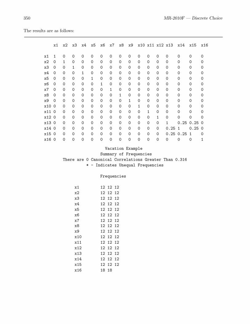
350 MR-2010F — Discrete Choice
The results are as follows:
x1 x2 x3 x4 x5 x6 x7 x8 x9 x10 x11 x12 x13 x14 x15 x16
x1 1 0 0 0 0 0 0 0 0 0 0 0 0 0 0 0x2 0 1 0 0 0 0 0 0 0 0 0 0 0 0 0 0x3 0 0 1 0 0 0 0 0 0 0 0 0 0 0 0 0x4 0 0 0 1 0 0 0 0 0 0 0 0 0 0 0 0x5 0 0 0 0 1 0 0 0 0 0 0 0 0 0 0 0x6 0 0 0 0 0 1 0 0 0 0 0 0 0 0 0 0x7 0 0 0 0 0 0 1 0 0 0 0 0 0 0 0 0x8 0 0 0 0 0 0 0 1 0 0 0 0 0 0 0 0x9 0 0 0 0 0 0 0 0 1 0 0 0 0 0 0 0x10 0 0 0 0 0 0 0 0 0 1 0 0 0 0 0 0x11 0 0 0 0 0 0 0 0 0 0 1 0 0 0 0 0x12 0 0 0 0 0 0 0 0 0 0 0 1 0 0 0 0x13 0 0 0 0 0 0 0 0 0 0 0 0 1 0.25 0.25 0x14 0 0 0 0 0 0 0 0 0 0 0 0 0.25 1 0.25 0x15 0 0 0 0 0 0 0 0 0 0 0 0 0.25 0.25 1 0x16 0 0 0 0 0 0 0 0 0 0 0 0 0 0 0 1
Vacation ExampleSummary of Frequencies
There are 0 Canonical Correlations Greater Than 0.316* - Indicates Unequal Frequencies
Frequencies
x1 12 12 12x2 12 12 12x3 12 12 12x4 12 12 12x5 12 12 12x6 12 12 12x7 12 12 12x8 12 12 12x9 12 12 12x10 12 12 12x11 12 12 12x12 12 12 12x13 12 12 12x14 12 12 12x15 12 12 12x16 18 18
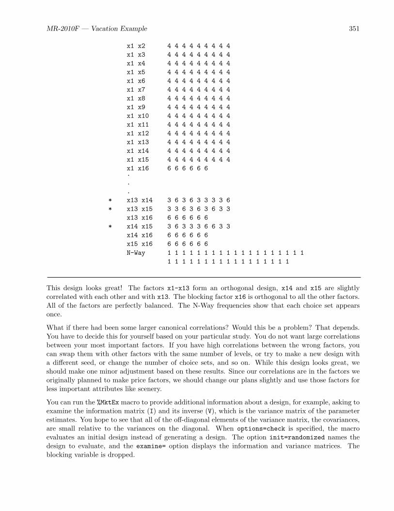
MR-2010F — Vacation Example 351
x1 x2 4 4 4 4 4 4 4 4 4x1 x3 4 4 4 4 4 4 4 4 4x1 x4 4 4 4 4 4 4 4 4 4x1 x5 4 4 4 4 4 4 4 4 4x1 x6 4 4 4 4 4 4 4 4 4x1 x7 4 4 4 4 4 4 4 4 4x1 x8 4 4 4 4 4 4 4 4 4x1 x9 4 4 4 4 4 4 4 4 4x1 x10 4 4 4 4 4 4 4 4 4x1 x11 4 4 4 4 4 4 4 4 4x1 x12 4 4 4 4 4 4 4 4 4x1 x13 4 4 4 4 4 4 4 4 4x1 x14 4 4 4 4 4 4 4 4 4x1 x15 4 4 4 4 4 4 4 4 4x1 x16 6 6 6 6 6 6...
* x13 x14 3 6 3 6 3 3 3 3 6* x13 x15 3 3 6 3 6 3 6 3 3
x13 x16 6 6 6 6 6 6* x14 x15 3 6 3 3 3 6 6 3 3
x14 x16 6 6 6 6 6 6x15 x16 6 6 6 6 6 6N-Way 1 1 1 1 1 1 1 1 1 1 1 1 1 1 1 1 1 1 1
1 1 1 1 1 1 1 1 1 1 1 1 1 1 1 1 1
This design looks great! The factors x1-x13 form an orthogonal design, x14 and x15 are slightlycorrelated with each other and with x13. The blocking factor x16 is orthogonal to all the other factors.All of the factors are perfectly balanced. The N-Way frequencies show that each choice set appearsonce.
What if there had been some larger canonical correlations? Would this be a problem? That depends.You have to decide this for yourself based on your particular study. You do not want large correlationsbetween your most important factors. If you have high correlations between the wrong factors, youcan swap them with other factors with the same number of levels, or try to make a new design witha different seed, or change the number of choice sets, and so on. While this design looks great, weshould make one minor adjustment based on these results. Since our correlations are in the factors weoriginally planned to make price factors, we should change our plans slightly and use those factors forless important attributes like scenery.
You can run the %MktEx macro to provide additional information about a design, for example, asking toexamine the information matrix (I) and its inverse (V), which is the variance matrix of the parameterestimates. You hope to see that all of the off-diagonal elements of the variance matrix, the covariances,are small relative to the variances on the diagonal. When options=check is specified, the macroevaluates an initial design instead of generating a design. The option init=randomized names thedesign to evaluate, and the examine= option displays the information and variance matrices. Theblocking variable is dropped.

352 MR-2010F — Discrete Choice
The following step creates the design:
%mktex(3 ** 15, /* all attrs of all alternatives */n=&n * &blocks, /* total number of choice sets */init=randomized(drop=x16), /* initial design */options=check, /* check initial design efficiency */examine=i v) /* show information & variance matrices */
A small part of the output is as follows:
Vacation Example
AveragePrediction
Design StandardNumber D-Efficiency A-Efficiency G-Efficiency Error------------------------------------------------------------------------
1 98.9099 97.8947 98.9418 0.9280
Vacation ExampleInformation Matrix
Intercept x11 x12 x21 x22 x31 x32 x41
Intercept 36.000 0 0 0 0 0 0 0x11 0 36.000 0 0 0 0 0 0x12 0 0 36.000 0 0 0 0 0x21 0 0 0 36.000 0 0 0 0x22 0 0 0 0 36.000 0 0 0x31 0 0 0 0 0 36.000 0 0x32 0 0 0 0 0 0 36.000 0x41 0 0 0 0 0 0 0 36.000
.
.
.
x122 36.000 0 0 0 0 0 0x131 0 36.000 0 9.000 0 -4.500 -7.794x132 0 0 36.000 0 9.000 -7.794 4.500x141 0 9.000 0 36.000 0 -4.500 -7.794x142 0 0 9.000 0 36.000 -7.794 4.500x151 0 -4.500 -7.794 -4.500 -7.794 36.000 0x152 0 -7.794 4.500 -7.794 4.500 0 36.000

MR-2010F — Vacation Example 353
Vacation ExampleVariance Matrix
Intercept x11 x12 x21 x22 x31 x32 x41
Intercept 0.028 0 0 0 0 0 0 0x11 0 0.028 0 0 0 0 0 0x12 0 0 0.028 0 0 0 0 0x21 0 0 0 0.028 0 0 0 0x22 0 0 0 0 0.028 0 0 0x31 0 0 0 0 0 0.028 0 0x32 0 0 0 0 0 0 0.028 0x41 0 0 0 0 0 0 0 0.028
.
.
.
x122 0.028 0 0 0 0 0 0x131 0 0.031 0 -0.006 0 0.003 0.005x132 0 0 0.031 0 -0.006 0.005 -0.003x141 0 -0.006 0 0.031 0 0.003 0.005x142 0 0 -0.006 0 0.031 0.005 -0.003x151 0 0.003 0.005 0.003 0.005 0.031 0x152 0 0.005 -0.003 0.005 -0.003 0 0.031
This design still looks good. The D-efficiency for the design excluding the blocking factor is 98.9099%.We can see that the nonorthogonality between x13-x15 makes their variances larger than the otherfactors (0.031 versus 0.028).
These next steps use the %MktLab macro to reassign the variable names, store the design in a permanentSAS data set, sasuser.VacationLinDesBlckd, and then use the %MktEx macro to check the results.See page 309 for more information about permanent SAS data sets. We need to make the correlatedvariables correspond to the least important attributes in different alternatives (in this case the sceneryfactors for Alaska, Mexico, and Maine). The vars= option provides the new variable names: the firstvariable (originally x1) becomes x1 (still), ..., the fifth variable (originally x5) becomes x5 (still), thesixth variable (originally x6) becomes x11, ... the tenth variable (originally x10) becomes x15, theeleventh through fifteenth original variables become x6, x9, x7, x8, x10, and finally the last variablebecomes Block. The following PROC SORT step sorts the design into blocks:
%mktlab(data=randomized, vars=x1-x5 x11-x15 x6 x9 x7 x8 x10 Block,out=sasuser.VacationLinDesBlckd)
proc sort data=sasuser.VacationLinDesBlckd; by block; run;
%mkteval(blocks=block)

354 MR-2010F — Discrete Choice
The output from the %MktLab macro, which shows the correspondence between the original and newvariable names is as follows:
Variable Mapping:x1 : x1x2 : x2x3 : x3x4 : x4x5 : x5x6 : x11x7 : x12x8 : x13x9 : x14x10 : x15x11 : x6x12 : x9x13 : x7x14 : x8x15 : x10x16 : Block
Some of the output from the %MktEval macro is as follows:
Vacation ExampleCanonical Correlations Between the Factors
There are 0 Canonical Correlations Greater Than 0.316
Block x1 x2 x3 x4 x5 x11 x12 x13 x14 x15 x6 x9 x7 x8 x10
Block 1 0 0 0 0 0 0 0 0 0 0 0 0 0 0 0x1 0 1 0 0 0 0 0 0 0 0 0 0 0 0 0 0x2 0 0 1 0 0 0 0 0 0 0 0 0 0 0 0 0x3 0 0 0 1 0 0 0 0 0 0 0 0 0 0 0 0x4 0 0 0 0 1 0 0 0 0 0 0 0 0 0 0 0x5 0 0 0 0 0 1 0 0 0 0 0 0 0 0 0 0x11 0 0 0 0 0 0 1 0 0 0 0 0 0 0 0 0x12 0 0 0 0 0 0 0 1 0 0 0 0 0 0 0 0x13 0 0 0 0 0 0 0 0 1 0 0 0 0 0 0 0x14 0 0 0 0 0 0 0 0 0 1 0 0 0 0 0 0x15 0 0 0 0 0 0 0 0 0 0 1 0 0 0 0 0x6 0 0 0 0 0 0 0 0 0 0 0 1 0 0 0 0x9 0 0 0 0 0 0 0 0 0 0 0 0 1 0 0 0x7 0 0 0 0 0 0 0 0 0 0 0 0 0 1 0.25 0.25x8 0 0 0 0 0 0 0 0 0 0 0 0 0 0.25 1 0.25x10 0 0 0 0 0 0 0 0 0 0 0 0 0 0.25 0.25 1

MR-2010F — Vacation Example 355
Vacation ExampleSummary of Frequencies
There are 0 Canonical Correlations Greater Than 0.316* - Indicates Unequal Frequencies
Frequencies
Block 18 18x1 12 12 12x2 12 12 12x3 12 12 12x4 12 12 12x5 12 12 12x11 12 12 12x12 12 12 12x13 12 12 12x14 12 12 12x15 12 12 12x6 12 12 12x9 12 12 12x7 12 12 12x8 12 12 12x10 12 12 12Block x1 6 6 6 6 6 6Block x2 6 6 6 6 6 6Block x3 6 6 6 6 6 6Block x4 6 6 6 6 6 6Block x5 6 6 6 6 6 6Block x11 6 6 6 6 6 6Block x12 6 6 6 6 6 6Block x13 6 6 6 6 6 6Block x14 6 6 6 6 6 6Block x15 6 6 6 6 6 6Block x6 6 6 6 6 6 6Block x9 6 6 6 6 6 6Block x7 6 6 6 6 6 6Block x8 6 6 6 6 6 6Block x10 6 6 6 6 6 6x1 x2 4 4 4 4 4 4 4 4 4x1 x3 4 4 4 4 4 4 4 4 4x1 x4 4 4 4 4 4 4 4 4 4x1 x5 4 4 4 4 4 4 4 4 4...

356 MR-2010F — Discrete Choice
* x7 x8 6 3 3 3 6 3 3 3 6* x7 x10 3 3 6 3 6 3 6 3 3* x8 x10 3 3 6 3 6 3 6 3 3
N-Way 1 1 1 1 1 1 1 1 1 1 1 1 1 1 1 1 1 1 11 1 1 1 1 1 1 1 1 1 1 1 1 1 1 1 1
From a Linear Arrangement to a Choice Design
These next steps prepare the design for analysis and further evaluation. We need to covert our lineararrangement into a choice design.∗ We need to create a data set Key that describes how the factors inour linear arrangement are used to make the choice design for analysis. The Key data set contains allof the factor names, x1, x2, x3, ... x15. We can run the %MktKey macro to get these names, for cuttingand pasting into the program without typing them. The following step requests 5 rows, 3 columns andthe results transposed so names progress down each column instead of across each row:
%mktkey(5 3 t)
The %MktKey macro produces the following data set:
x1 x2 x3
x1 x6 x11x2 x7 x12x3 x8 x13x4 x9 x14x5 x10 x15
∗See page 67 for an explanation of the linear arrangement of a choice design versus the arrangement of a choice designthat is more suitable for analysis.
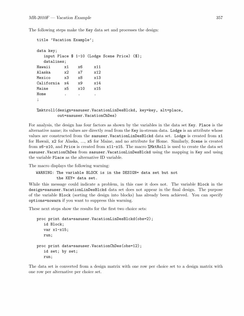
MR-2010F — Vacation Example 357
The following steps make the Key data set and processes the design:
title ’Vacation Example’;
data key;input Place $ 1-10 (Lodge Scene Price) ($);datalines;
Hawaii x1 x6 x11Alaska x2 x7 x12Mexico x3 x8 x13California x4 x9 x14Maine x5 x10 x15Home . . .;
%mktroll(design=sasuser.VacationLinDesBlckd, key=key, alt=place,out=sasuser.VacationChDes)
For analysis, the design has four factors as shown by the variables in the data set Key. Place is thealternative name; its values are directly read from the Key in-stream data. Lodge is an attribute whosevalues are constructed from the sasuser.VacationLinDesBlckd data set. Lodge is created from x1for Hawaii, x2 for Alaska, ..., x5 for Maine, and no attribute for Home. Similarly, Scene is createdfrom x6-x10, and Price is created from x11-x15. The macro %MktRoll is used to create the data setsasuser.VacationChDes from sasuser.VacationLinDesBlckd using the mapping in Key and usingthe variable Place as the alternative ID variable.
The macro displays the following warning:
WARNING: The variable BLOCK is in the DESIGN= data set but notthe KEY= data set.
While this message could indicate a problem, in this case it does not. The variable Block in thedesign=sasuser.VacationLinDesBlckd data set does not appear in the final design. The purposeof the variable Block (sorting the design into blocks) has already been achieved. You can specifyoptions=nowarn if you want to suppress this warning.
These next steps show the results for the first two choice sets:
proc print data=sasuser.VacationLinDesBlckd(obs=2);id Block;var x1-x15;run;
proc print data=sasuser.VacationChDes(obs=12);id set; by set;run;
The data set is converted from a design matrix with one row per choice set to a design matrix withone row per alternative per choice set.

358 MR-2010F — Discrete Choice
The results are as follows:
Vacation Example
Block x1 x2 x3 x4 x5 x6 x7 x8 x9 x10 x11 x12 x13 x14 x15
1 1 3 3 1 1 3 1 3 2 1 1 1 2 2 21 1 2 1 2 3 3 2 2 1 3 1 3 1 1 2
Vacation Example
Set Place Lodge Scene Price
1 Hawaii 1 3 1Alaska 3 1 1Mexico 3 3 2California 1 2 2Maine 1 1 2Home . . .
2 Hawaii 1 3 1Alaska 2 2 3Mexico 1 2 1California 2 1 1Maine 3 3 2Home . . .
The following steps assign formats, convert the variable Price to contain actual prices, and recode theconstant alternative:
proc format;value price 1 = ’ 999’ 2 = ’1249’
3 = ’1499’ 0 = ’ 0’;value scene 1 = ’Mountains’ 2 = ’Lake’
3 = ’Beach’ 0 = ’Home’;value lodge 1 = ’Cabin’ 2 = ’Bed & Breakfast’
3 = ’Hotel’ 0 = ’Home’;run;
data sasuser.VacationChDes;set sasuser.VacationChDes;if place = ’Home’ then do; lodge = 0; scene = 0; price = 0; end;price = input(put(price, price.), 5.);format scene scene. lodge lodge.;run;
proc print data=sasuser.VacationChDes(obs=12);id set; by set;run;

MR-2010F — Vacation Example 359
The results are as follows:
Vacation Example
Set Place Lodge Scene Price
1 Hawaii Cabin Beach 999Alaska Hotel Mountains 999Mexico Hotel Beach 1249California Cabin Lake 1249Maine Cabin Mountains 1249Home Home Home 0
2 Hawaii Cabin Beach 999Alaska Bed & Breakfast Lake 1499Mexico Cabin Lake 999California Bed & Breakfast Mountains 999Maine Hotel Beach 1249Home Home Home 0
It is not necessary to recode the missing values for the constant alternative. In practice, we usually donot do this step. However, for this first analysis, we want all nonmissing values of the attributes so wecan see all levels in the final displayed output. We also recode Price so that for a later analysis, we cananalyze Price as a quantitative effect. For example, the expression put(price, price.) converts anumber, say 2, into a string (in this case ’1249’), then the input function reads the string and convertsit to a numeric 1249.

360 MR-2010F — Discrete Choice
Testing the Design Before Data Collection
Collecting data is time consuming and expensive. It is always good practice to make sure that thedesign works with the most complicated model that we anticipate fitting. The following steps evaluatethe choice design:
title2 ’Evaluate the Choice Design’;
%choiceff(data=sasuser.VacationChDes,/* candidate set of choice sets */init=sasuser.VacationChDes(keep=set), /* select these sets */intiter=0, /* evaluate without internal iterations */
/* alternative-specific effects model *//* zero=none - use all levels of place *//* order=data - do not sort levels */
model=class(place / zero=none order=data)/* place * price ... - interactions or *//* alternative-specific effects */
class(place * price place * scene place * lodge /zero=none /* zero=none - use all levels of place */order=formatted) / /* order=formatted - sort levels */
lprefix=0 /* lpr=0 labels created from just levels*/cprefix=0 /* cpr=0 names created from just levels */separators=’ ’ ’, ’,/* use comma sep to build interact terms*/
nsets=36, /* number of choice sets */nalts=6, /* number of alternatives */beta=zero) /* assumed beta vector, Ho: b=0 */
The %ChoicEff macro has two uses. You can use it to search for an efficient choice design, or you canuse it to evaluate a choice design including designs that are generated using other methods such as the%MktEx macro. It is this latter use that is illustrated here.

MR-2010F — Vacation Example 361
The way you check a design like this is to first name it in the data= option. This is the candidate setthat contains all of the choice sets that we will consider. In addition, the same design is named in theinit= option. Just the variable Set is kept. It is used to bring in just the indicated choice sets fromthe data= design, which in this case is all of them. The option nsets= specifies that there are 36 choicesets, and nalts= specifies that there are 6 alternatives. The option beta=zero specifies that we areassuming for design evaluation purposes the null hypothesis that all of the betas or part-worth utilitiesare zero. You can evaluate the design for other parameter vectors by specifying a list of numbers afterbeta=. This will change the variances and standard errors. We also specify intiter=0 which specifieszero internal iterations. We use zero internal iterations when we want to evaluate an initial design, butnot attempt to improve it. The last option specifies the model.
The model specification contains everything that appears in the TRANSREG procedure’s modelstatement for coding the design. Some of these options are familiar from the previous example.The specification class(place / zero=none order=data) names the place variable as a classifi-cation variables and asks for coded variables for every level including the constant, stay-at-homealternative. The specification class(place * price place * scene place * lodge / zero=noneorder=formatted) asks for alternative-specific effects for price, lodging, and scenery. The alternative-specific effects permit the part-worth utilities to be different for each of the destinations. This isaccomplished by requesting interactions between the destination and the attributes. Class levels aresorted by their formatted values, and for all factors. The zero=none option is used so that for now wecan see all of the levels of all of the factors. Many of these will not correspond to estimable parameters,and we can eliminate them later. See page 78 for more information about the zero= option.
The lprefix=0 option specifies that when labels are created for the binary variables, zero charactersof the original variable name should be used as a prefix. The cprefix=0 option specifies that whennames are created for the binary variables, zero characters of the original variable name should beused as a prefix. The separators=’ ’ ’, ’ option provides two strings (one blank and the other acomma followed by a blank) that let you specify label component separators for the main effect andinteraction terms. By specifying a comma and a blank for the second value, we request labels for theside trip effects like ’Alaska, 999’ instead of the default ’Alaska * 999’. This option is explainedin more detail on page 449.
The last tables from the %ChoicEff macro, which are the ones in which we are most interested, is asfollows:
Vacation ExampleEvaluate the Choice Design
Final Results
Design 1Choice Sets 36Alternatives 6Parameters 35Maximum Parameters 180D-Efficiency 0D-Error .
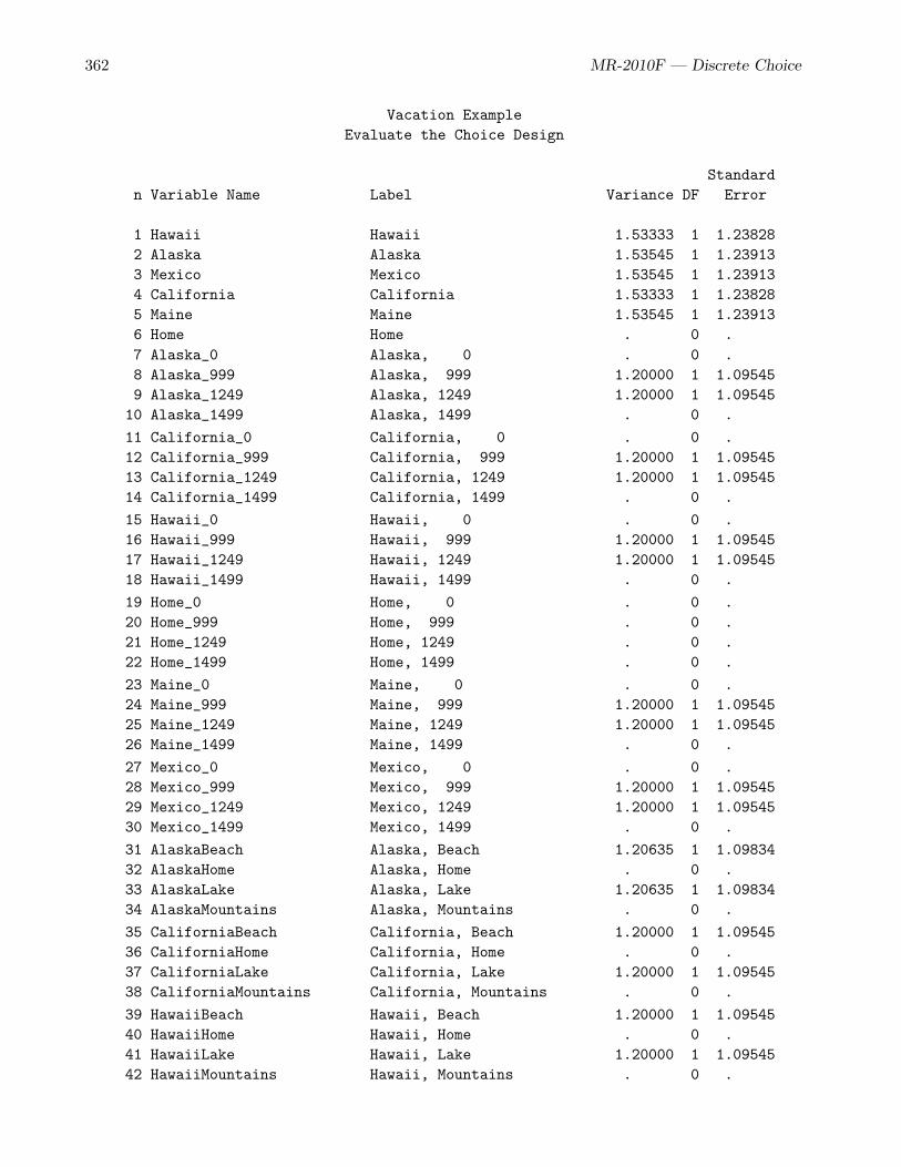
362 MR-2010F — Discrete Choice
Vacation ExampleEvaluate the Choice Design
Standardn Variable Name Label Variance DF Error
1 Hawaii Hawaii 1.53333 1 1.238282 Alaska Alaska 1.53545 1 1.239133 Mexico Mexico 1.53545 1 1.239134 California California 1.53333 1 1.238285 Maine Maine 1.53545 1 1.239136 Home Home . 0 .7 Alaska_0 Alaska, 0 . 0 .8 Alaska_999 Alaska, 999 1.20000 1 1.095459 Alaska_1249 Alaska, 1249 1.20000 1 1.0954510 Alaska_1499 Alaska, 1499 . 0 .
11 California_0 California, 0 . 0 .12 California_999 California, 999 1.20000 1 1.0954513 California_1249 California, 1249 1.20000 1 1.0954514 California_1499 California, 1499 . 0 .
15 Hawaii_0 Hawaii, 0 . 0 .16 Hawaii_999 Hawaii, 999 1.20000 1 1.0954517 Hawaii_1249 Hawaii, 1249 1.20000 1 1.0954518 Hawaii_1499 Hawaii, 1499 . 0 .
19 Home_0 Home, 0 . 0 .20 Home_999 Home, 999 . 0 .21 Home_1249 Home, 1249 . 0 .22 Home_1499 Home, 1499 . 0 .
23 Maine_0 Maine, 0 . 0 .24 Maine_999 Maine, 999 1.20000 1 1.0954525 Maine_1249 Maine, 1249 1.20000 1 1.0954526 Maine_1499 Maine, 1499 . 0 .
27 Mexico_0 Mexico, 0 . 0 .28 Mexico_999 Mexico, 999 1.20000 1 1.0954529 Mexico_1249 Mexico, 1249 1.20000 1 1.0954530 Mexico_1499 Mexico, 1499 . 0 .
31 AlaskaBeach Alaska, Beach 1.20635 1 1.0983432 AlaskaHome Alaska, Home . 0 .33 AlaskaLake Alaska, Lake 1.20635 1 1.0983434 AlaskaMountains Alaska, Mountains . 0 .
35 CaliforniaBeach California, Beach 1.20000 1 1.0954536 CaliforniaHome California, Home . 0 .37 CaliforniaLake California, Lake 1.20000 1 1.0954538 CaliforniaMountains California, Mountains . 0 .
39 HawaiiBeach Hawaii, Beach 1.20000 1 1.0954540 HawaiiHome Hawaii, Home . 0 .41 HawaiiLake Hawaii, Lake 1.20000 1 1.0954542 HawaiiMountains Hawaii, Mountains . 0 .
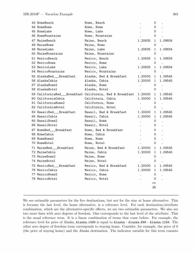
MR-2010F — Vacation Example 363
43 HomeBeach Home, Beach . 0 .44 HomeHome Home, Home . 0 .45 HomeLake Home, Lake . 0 .46 HomeMountains Home, Mountains . 0 .
47 MaineBeach Maine, Beach 1.20635 1 1.0983448 MaineHome Maine, Home . 0 .49 MaineLake Maine, Lake 1.20635 1 1.0983450 MaineMountains Maine, Mountains . 0 .
51 MexicoBeach Mexico, Beach 1.20635 1 1.0983452 MexicoHome Mexico, Home . 0 .53 MexicoLake Mexico, Lake 1.20635 1 1.0983454 MexicoMountains Mexico, Mountains . 0 .
55 AlaskaBed___Breakfast Alaska, Bed & Breakfast 1.20000 1 1.0954556 AlaskaCabin Alaska, Cabin 1.20000 1 1.0954557 AlaskaHome2 Alaska, Home . 0 .58 AlaskaHotel Alaska, Hotel . 0 .
59 CaliforniaBed___Breakfast California, Bed & Breakfast 1.20000 1 1.0954560 CaliforniaCabin California, Cabin 1.20000 1 1.0954561 CaliforniaHome2 California, Home . 0 .62 CaliforniaHotel California, Hotel . 0 .
63 HawaiiBed___Breakfast Hawaii, Bed & Breakfast 1.20000 1 1.0954564 HawaiiCabin Hawaii, Cabin 1.20000 1 1.0954565 HawaiiHome2 Hawaii, Home . 0 .66 HawaiiHotel Hawaii, Hotel . 0 .
67 HomeBed___Breakfast Home, Bed & Breakfast . 0 .68 HomeCabin Home, Cabin . 0 .69 HomeHome2 Home, Home . 0 .70 HomeHotel Home, Hotel . 0 .
71 MaineBed___Breakfast Maine, Bed & Breakfast 1.20000 1 1.0954572 MaineCabin Maine, Cabin 1.20000 1 1.0954573 MaineHome2 Maine, Home . 0 .74 MaineHotel Maine, Hotel . 0 .
75 MexicoBed___Breakfast Mexico, Bed & Breakfast 1.20000 1 1.0954576 MexicoCabin Mexico, Cabin 1.20000 1 1.0954577 MexicoHome2 Mexico, Home . 0 .78 MexicoHotel Mexico, Hotel . 0 .
==35
We see estimable parameters for the five destinations, but not for the stay at home alternative. Thisis because the last level, the home alternative, is a reference level. For each destination/attributecombination, which are the alternative-specific effects, we see two estimable parameters. We also seetwo more lines with zero degrees of freedom. One corresponds to the last level of the attribute. Thisis the usual reference term. It is a linear combination of terms that come before. For example, thereference level for price of Alaska, Alaska 1499 is equal to Alaska - Alaska 999 - Alaska 1249. Theother zero degree of freedom term corresponds to staying home. Consider, for example, the price of 0(the price of staying home) and the Alaska destination. The indicator variable for this term consists

364 MR-2010F — Discrete Choice
of all zeros since the price of 0 never happens with Alaska. So there is no parameter to estimate. Youcan prove these things to yourself by examining the coded design. The %ChoicEff macro makes itavailable in a SAS data set called tmp cand. This data set is not considered to be one of the “normal”output data sets from the macro, so no note is created about its creation. However, it is always therein case you want to look at it. You can verify that Alaska 1499 is equal to Alaska - Alaska 999 -Alaska 1249 as follows:
proc reg data=tmp_cand;model Alaska_1499 = Alaska Alaska_999 Alaska_1249 / noint;run; quit;
The results are as follows:
Vacation ExampleEvaluate the Choice Design
The REG ProcedureModel: MODEL1
Dependent Variable: Alaska_1499 Alaska, 1499
Number of Observations Read 216Number of Observations Used 216
NOTE: No intercept in model. R-Square is redefined.
Analysis of Variance
Sum of MeanSource DF Squares Square F Value Pr > F
Model 3 12.00000 4.00000 Infty <.0001Error 213 0 0Uncorrected Total 216 12.00000
Root MSE 0 R-Square 1.0000Dependent Mean 0.05556 Adj R-Sq 1.0000Coeff Var 0
Parameter Estimates
Parameter StandardVariable Label DF Estimate Error t Value Pr > |t|
Alaska Alaska 1 1.00000 0 Infty <.0001Alaska_999 Alaska, 999 1 -1.00000 0 -Infty <.0001Alaska_1249 Alaska, 1249 1 -1.00000 0 -Infty <.0001
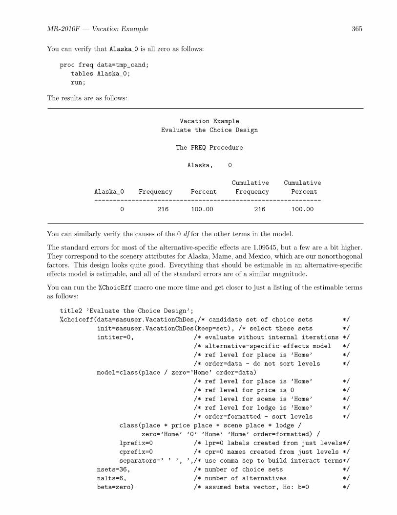
MR-2010F — Vacation Example 365
You can verify that Alaska 0 is all zero as follows:
proc freq data=tmp_cand;tables Alaska_0;run;
The results are as follows:
Vacation ExampleEvaluate the Choice Design
The FREQ Procedure
Alaska, 0
Cumulative CumulativeAlaska_0 Frequency Percent Frequency Percent-------------------------------------------------------------
0 216 100.00 216 100.00
You can similarly verify the causes of the 0 df for the other terms in the model.
The standard errors for most of the alternative-specific effects are 1.09545, but a few are a bit higher.They correspond to the scenery attributes for Alaska, Maine, and Mexico, which are our nonorthogonalfactors. This design looks quite good. Everything that should be estimable in an alternative-specificeffects model is estimable, and all of the standard errors are of a similar magnitude.
You can run the %ChoicEff macro one more time and get closer to just a listing of the estimable termsas follows:
title2 ’Evaluate the Choice Design’;%choiceff(data=sasuser.VacationChDes,/* candidate set of choice sets */
init=sasuser.VacationChDes(keep=set), /* select these sets */intiter=0, /* evaluate without internal iterations */
/* alternative-specific effects model *//* ref level for place is ’Home’ *//* order=data - do not sort levels */
model=class(place / zero=’Home’ order=data)/* ref level for place is ’Home’ *//* ref level for price is 0 *//* ref level for scene is ’Home’ *//* ref level for lodge is ’Home’ *//* order=formatted - sort levels */
class(place * price place * scene place * lodge /zero=’Home’ ’0’ ’Home’ ’Home’ order=formatted) /
lprefix=0 /* lpr=0 labels created from just levels*/cprefix=0 /* cpr=0 names created from just levels */separators=’ ’ ’, ’,/* use comma sep to build interact terms*/
nsets=36, /* number of choice sets */nalts=6, /* number of alternatives */beta=zero) /* assumed beta vector, Ho: b=0 */

366 MR-2010F — Discrete Choice
The results of this step are not shown, but there are 35 model df like before and many fewer zeros.The macro displays a list of the terms with zero df. In this case, the list is as follows:
Alaska_1499 California_1499 Hawaii_1499 Maine_1499 Mexico_1499 AlaskaMountainsCaliforniaMountains HawaiiMountains MaineMountains MexicoMountains AlaskaHotelCaliforniaHotel HawaiiHotel MaineHotel MexicoHotel
You can incorporate this list into the macro as follows:
title2 ’Evaluate the Choice Design’;
%choiceff(data=sasuser.VacationChDes,/* candidate set of choice sets */init=sasuser.VacationChDes(keep=set), /* select these sets */intiter=0, /* evaluate without internal iterations */
/* alternative-specific effects model *//* ref level for place is ’Home’ *//* order=data - do not sort levels */
model=class(place / zero=’Home’ order=data)/* ref level for place is ’Home’ *//* ref level for price is 0 *//* ref level for scene is ’Home’ *//* ref level for lodge is ’Home’ *//* order=formatted - sort levels */
class(place * price place * scene place * lodge /zero=’Home’ ’0’ ’Home’ ’Home’ order=formatted) /
lprefix=0 /* lpr=0 labels created from just levels*/cprefix=0 /* cpr=0 names created from just levels */separators=’ ’ ’, ’,/* use comma sep to build interact terms*/
nsets=36, /* number of choice sets */nalts=6, /* number of alternatives */
/* extra model terms to drop from model */drop=Alaska_1499 California_1499 Hawaii_1499 Maine_1499
Mexico_1499 AlaskaMountains CaliforniaMountainsHawaiiMountains MaineMountains MexicoMountains AlaskaHotelCaliforniaHotel HawaiiHotel MaineHotel MexicoHotel,
beta=zero) /* assumed beta vector, Ho: b=0 */
Most of the results are as follows:
Vacation ExampleEvaluate the Choice Design
Design Iteration D-Efficiency D-Error----------------------------------------------
1 0 1.18690 * 0.84253

MR-2010F — Vacation Example 367
Vacation ExampleEvaluate the Choice Design
Final Results
Design 1Choice Sets 36Alternatives 6Parameters 35Maximum Parameters 180D-Efficiency 1.1869D-Error 0.8425
Vacation ExampleEvaluate the Choice Design
Standardn Variable Name Label Variance DF Error
1 Hawaii Hawaii 1.53333 1 1.238282 Alaska Alaska 1.53545 1 1.239133 Mexico Mexico 1.53545 1 1.239134 California California 1.53333 1 1.238285 Maine Maine 1.53545 1 1.239136 Alaska_999 Alaska, 999 1.20000 1 1.095457 Alaska_1249 Alaska, 1249 1.20000 1 1.09545
8 California_999 California, 999 1.20000 1 1.095459 California_1249 California, 1249 1.20000 1 1.09545
10 Hawaii_999 Hawaii, 999 1.20000 1 1.0954511 Hawaii_1249 Hawaii, 1249 1.20000 1 1.09545
12 Maine_999 Maine, 999 1.20000 1 1.0954513 Maine_1249 Maine, 1249 1.20000 1 1.09545
14 Mexico_999 Mexico, 999 1.20000 1 1.0954515 Mexico_1249 Mexico, 1249 1.20000 1 1.09545
16 AlaskaBeach Alaska, Beach 1.20635 1 1.0983417 AlaskaLake Alaska, Lake 1.20635 1 1.09834
18 CaliforniaBeach California, Beach 1.20000 1 1.0954519 CaliforniaLake California, Lake 1.20000 1 1.09545
20 HawaiiBeach Hawaii, Beach 1.20000 1 1.0954521 HawaiiLake Hawaii, Lake 1.20000 1 1.09545
22 MaineBeach Maine, Beach 1.20635 1 1.0983423 MaineLake Maine, Lake 1.20635 1 1.09834
24 MexicoBeach Mexico, Beach 1.20635 1 1.0983425 MexicoLake Mexico, Lake 1.20635 1 1.09834
26 AlaskaBed___Breakfast Alaska, Bed & Breakfast 1.20000 1 1.0954527 AlaskaCabin Alaska, Cabin 1.20000 1 1.09545
28 CaliforniaBed___Breakfast California, Bed & Breakfast 1.20000 1 1.0954529 CaliforniaCabin California, Cabin 1.20000 1 1.09545

368 MR-2010F — Discrete Choice
30 HawaiiBed___Breakfast Hawaii, Bed & Breakfast 1.20000 1 1.0954531 HawaiiCabin Hawaii, Cabin 1.20000 1 1.09545
32 MaineBed___Breakfast Maine, Bed & Breakfast 1.20000 1 1.0954533 MaineCabin Maine, Cabin 1.20000 1 1.09545
34 MexicoBed___Breakfast Mexico, Bed & Breakfast 1.20000 1 1.0954535 MexicoCabin Mexico, Cabin 1.20000 1 1.09545
==35
Now we have all of the final 35 parameters. We used the drop= option to drop the extra terms. It isoften the case with a choice model with a constant alternative that it is hard to write a model thatprecisely creates all of the right terms with nothing extra. The drop= option gives you a way to toremove the extra terms.
These results look good. The variances for Alaska, Mexico, and Maine are slightly larger than thevariances for Hawaii and California. Similarly, the variances for the scenery parameters for Alaska,Mexico, and Maine are larger than the variances for the other attributes. This is because we have asmall amount of nonorthogonality in those attributes. You can see that this effect is slight.
There is one more test that should be run before a design is used. The following %MktDups macro stepchecks the design to see if any choice sets are duplicates of any other choice sets:
%mktdups(branded, data=sasuser.VacationChDes,nalts=6, factors=place price scene lodge)
The results are as follows:
Design: BrandedFactors: place price scene lodge
PlaceLodge Price Scene
Duplicate Sets: 0
The first line of the table tells us that this is a branded design as opposed to a generic design (bundlesof attributes with no brands). The second line tells us the factors as specified in the factors= option.These are followed by the actual variable names for the factors. The last line reports the number ofduplicates. In this case, there are no duplicate choice sets. If there are duplicate choice sets, thenchanging the random number seed might help. Changing other aspects of the design or the approachfor making the design might also help.

MR-2010F — Vacation Example 369
Generating the Questionnaire
The following DATA step produces the questionnaires:
title;proc sort data=sasuser.VacationLinDesBlckd; by block; run;
options ls=80 ps=60 nodate nonumber;
data _null_;array dests[&mm1] $ 10 _temporary_ (’Hawaii’ ’Alaska’ ’Mexico’
’California’ ’Maine’);array prices[3] $ 5 _temporary_ (’$999’ ’$1249’ ’$1499’);array scenes[3] $ 13 _temporary_
(’the Mountains’ ’a Lake’ ’the Beach’);array lodging[3] $ 15 _temporary_
(’Cabin’ ’Bed & Breakfast’ ’Hotel’);array x[15];
file print linesleft=ll;
set sasuser.VacationLinDesBlckd;by block;
if first.block then do;choice = 0;put _page_;put @50 ’Form: ’ block ’ Subject: ________’ //;end;
choice + 1;
if ll < 19 then put _page_;put choice 2. ’) Circle your choice of ’
’vacation destinations:’ /;do dest = 1 to &mm1;
put ’ ’ dest 1. ’) ’ dests[dest]+(-1) ’, staying in a ’ lodging[x[dest]]’near ’ scenes[x[&mm1 + dest]] +(-1) ’,’ /’ with a package cost of ’prices[x[2 * &mm1 + dest]] +(-1) ’.’ /;
end;put " &m) Stay at home this year." /;run;
They are then copied and the data are collected. In this design, there are five destinations, andeach destination has three attributes. Each destination name is accessed from the array dests. Notethat destination is not a factor in the design; it is a bin into which the attributes are grouped. Thefactors in the design are named in the statement array x[15], which is a short-hand notation forarray x[15] x1-x15. The first five factors are used for the lodging attribute of the five destinations.The actual descriptions of lodging are accessed by lodging[x[dest]]. The variable Dest varies from1 to 5 destinations, so x[dest] extracts the levels for the Dest destination. Similarly for scenery,

370 MR-2010F — Discrete Choice
scenes[x[&mm1 + dest]] extracts the descriptions of the scenery. The index &mm1 + dest accessesfactors 6 through 10, and x[&mm1 + dest] indexes the scenes array. For prices, prices[x[2 * &mm1+ dest]], the index 2 * &mm1 + dest accesses the factors 11 through 15.
The first two choice sets are as follows:
Vacation ExampleForm: 1 Subject: ________
1) Circle your choice of vacation destinations:
1) Hawaii, staying in a Cabin near the Beach,with a package cost of $999.
2) Alaska, staying in a Hotel near the Mountains,with a package cost of $999.
3) Mexico, staying in a Hotel near the Beach,with a package cost of $1249.
4) California, staying in a Cabin near a Lake,with a package cost of $1249.
5) Maine, staying in a Cabin near the Mountains,with a package cost of $1249.
6) Stay at home this year.
2) Circle your choice of vacation destinations:
1) Hawaii, staying in a Cabin near the Beach,with a package cost of $999.
2) Alaska, staying in a Bed & Breakfast near a Lake,with a package cost of $1499.
3) Mexico, staying in a Cabin near a Lake,with a package cost of $999.
4) California, staying in a Bed & Breakfast near the Mountains,with a package cost of $999.
5) Maine, staying in a Hotel near the Beach,with a package cost of $1249.
6) Stay at home this year.

MR-2010F — Vacation Example 371
In practice, data collection is typically much more elaborate than this. It might involve art work orphotographs, and the choice sets might be presented and the data might be collected through personalinterview or over the Web. However the choice sets are presented and the data are collected, theessential elements remain the same. Subjects are shown a set of alternatives and are asked to make achoice, then they go on to the next set.
Entering and Processing the Data
The data are read as follows:
title ’Vacation Example’;
data results;input Subj Form (choose1-choose&n) (1.) @@;datalines;
1 1 111353313351554151 2 2 344113155513111413 3 1 1323533311515341514 2 341133131523331143 5 1 142153111151334143 6 2 3441141115431311517 1 141343111311154154 8 2 344113111343121111 9 1 14112413115134215510 2 344113131523131141 11 1 311423131353524144 12 2 33212315141333115113 1 311244331352134155 14 2 341114111543131153 15 1 14125311135134415116 2 344135131323331143 17 1 142123313154132141 18 2 54211315132313114119 1 145314111311144111 20 2 344111131313431143 21 1 133343131313432145...;
Data from a total of 200 subjects are collected, 100 per form.
Next, we use the %MktMerge macro as follows to combine the data and design and create the variablec, indicating whether each alternative is a first choice or a subsequent choice:
%mktmerge(design=sasuser.VacationChDes, data=results, out=res2, blocks=form,nsets=&n, nalts=&m, setvars=choose1-choose&n)
proc print data=res2(obs=12);id subj form set; by subj form set;run;
This macro takes the design=sasuser.VacationChDes experimental design, merges it with the data=result data set, creating the out=res2 output data set. The Results data set contains the variableForm that contains the block number. Since there are two blocks, this variable must have values of 1and 2. This variable must be specified in the blocks= option. The experiment has nsets=&n choicesets, nalts=6 alternatives, and the variables setvars=choose1-choose&n contain the numbers of thechosen alternatives. The output data set Res2 has 21,600 observations (200 subjects who each saw 18choice sets with 6 alternatives).

372 MR-2010F — Discrete Choice
The first two choice sets are as follows:
Vacation Example
Subj Form Set Place Lodge Scene Price c
1 1 1 Hawaii Cabin Beach 999 1Alaska Hotel Mountains 999 2Mexico Hotel Beach 1249 2California Cabin Lake 1249 2Maine Cabin Mountains 1249 2Home Home Home 0 2
1 1 2 Hawaii Cabin Beach 999 1Alaska Bed & Breakfast Lake 1499 2Mexico Cabin Lake 999 2California Bed & Breakfast Mountains 999 2Maine Hotel Beach 1249 2Home Home Home 0 2
Binary Coding
One more thing must be done to these data before they can be analyzed. The binary design matrix iscoded for each effect. This can be done with PROC TRANSREG as follows:
proc transreg design=5000 data=res2 nozeroconstant norestoremissing;model class(place / zero=none order=data)
class(price scene lodge / zero=none order=formatted) /lprefix=0;
output out=coded(drop=_type_ _name_ intercept);id subj set form c;run;
The design option specifies that no model is fit; the procedure is just being used to code a design.When design is specified, dependent variables are not required. Optionally, design can be followed by“=n” where n is the number of observations to process at one time. By default, PROC TRANSREGcodes all observations in one big group. For very large data sets, this can consume large amountsof memory and time. Processing blocks of smaller numbers of observations is more computationallyefficient. The option design=5000 processes observations in blocks of 5000. For smaller computers,try something like design=1000.
The nozeroconstant and norestoremissing options are not necessary for this example but are in-cluded here because sometimes they are very helpful in coding choice models. The nozeroconstant op-tion specifies that if the coding creates a constant variable, it should not be zeroed. The nozeroconstantoption should always be specified when you specify design=n because the last group of observationsmight be small and might contain constant variables. The nozeroconstant option is also importantif you do something like coding by subj set because sometimes an attribute is constant within a

MR-2010F — Vacation Example 373
choice set. The norestoremissing option specifies that missing values should not be restored whenthe out= data set is created. By default, the coded class variable contains a row of missing valuesfor observations in which the class variable is missing. With the norestoremissing option, theseobservations contain a row of zeros instead. This option is useful when there is a constant alternativeindicated by missing values. Both of these options, like almost all options in PROC TRANSREG, canbe abbreviated to three characters (noz and nor).
The model statement names the variables to code and provides information about how they shouldbe coded. The specification class(place / ...) specifies that the variable Place is a classificationvariable and requests a binary coding. The zero=none option creates binary variables for all categories.The order=data option sorts the levels into the order they are encountered in the data set. It is specifiedso ’Home’ is the last destination in the analysis, as it is in the data set. The class(price scene lodge/ ...) specification names the variables Price, Scene, and Lodge as categorical variables and createsbinary variables for all of the levels of all of the variables. The levels are sorted into order based ontheir formatted values. The lprefix=0 option specifies that when labels are created for the binaryvariables, zero characters of the original variable name should be used as a prefix. This means that thelabels are created only from the level values. For example, ’Mountains’ and ’Bed & Breakfast’ arecreated as labels not ’Scene Mountains’ and ’Lodge Bed & Breakfast’.
An output statement names the output data set and drops variables that are not needed. Thesevariables do not have to be dropped. However, since they are variable names that are often found inspecial data set types, PROC PHREG displays warnings when it finds them. Dropping the variablesprevents the warnings. Finally, the id statement names the additional variables that we want copiedfrom the input to the output data set. The following steps display the first coded choice set:
proc print data=coded(obs=6);id place;var subj set form c price scene lodge;run;
proc print data=coded(obs=6) label;var pl:;run;
proc print data=coded(obs=6) label;id place;var sc:;run;
proc print data=coded(obs=6) label;id place;var lo: pr:;run;
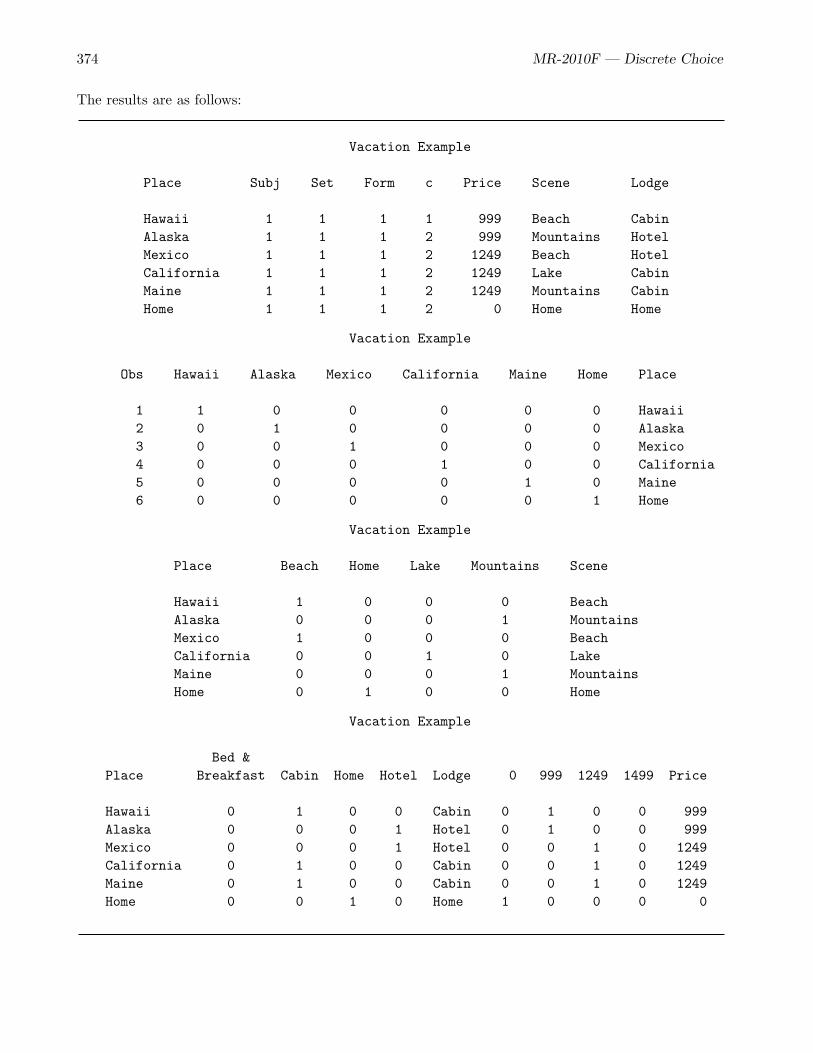
374 MR-2010F — Discrete Choice
The results are as follows:
Vacation Example
Place Subj Set Form c Price Scene Lodge
Hawaii 1 1 1 1 999 Beach CabinAlaska 1 1 1 2 999 Mountains HotelMexico 1 1 1 2 1249 Beach HotelCalifornia 1 1 1 2 1249 Lake CabinMaine 1 1 1 2 1249 Mountains CabinHome 1 1 1 2 0 Home Home
Vacation Example
Obs Hawaii Alaska Mexico California Maine Home Place
1 1 0 0 0 0 0 Hawaii2 0 1 0 0 0 0 Alaska3 0 0 1 0 0 0 Mexico4 0 0 0 1 0 0 California5 0 0 0 0 1 0 Maine6 0 0 0 0 0 1 Home
Vacation Example
Place Beach Home Lake Mountains Scene
Hawaii 1 0 0 0 BeachAlaska 0 0 0 1 MountainsMexico 1 0 0 0 BeachCalifornia 0 0 1 0 LakeMaine 0 0 0 1 MountainsHome 0 1 0 0 Home
Vacation Example
Bed &Place Breakfast Cabin Home Hotel Lodge 0 999 1249 1499 Price
Hawaii 0 1 0 0 Cabin 0 1 0 0 999Alaska 0 0 0 1 Hotel 0 1 0 0 999Mexico 0 0 0 1 Hotel 0 0 1 0 1249California 0 1 0 0 Cabin 0 0 1 0 1249Maine 0 1 0 0 Cabin 0 0 1 0 1249Home 0 0 1 0 Home 1 0 0 0 0

MR-2010F — Vacation Example 375
The coded design consists of binary variables for destinations Hawaii — Home, scenery Beach —Mountains, lodging Bed & Breakfast — Hotel, and price 0 — 1499. For example, in the last panel ofthe first choice set, the Cabin column has a 1 for Hawaii since Hawaii has Cabin lodging in this choiceset. The Cabin column has a 0 for Alaska since Alaska does not have Cabin lodging in this choice set.These binary variables form the independent variables in the analysis.
Note that we are fitting a model with generic attributes. Generic attributes are assumed to be thesame for all alternatives. For example, our model is structured so that the part-worth utility for beingon a lake is the same for Hawaii, Alaska, and all of the other destinations. Similarly, the part-worthutilities for the different prices do not depend on the destinations. In contrast, on page 386, using thesame data, we code alternative-specific effects where the part-worth utilities are allowed by the modelto be different for each of the destinations.
PROC PHREG is run to fit the choice model as follows:
proc phreg data=coded brief;model c*c(2) = &_trgind / ties=breslow;strata subj set;run;
We specify the & trgind macro variable for the model statement independent variable list. PROCTRANSREG automatically creates this macro variable. It contains the list of coded independentvariables generated by the procedure. This is so you do not have to figure out what names TRANSREGcreated and specify them. In this case, PROC TRANSREG sets & trgind to contain the following list:
PlaceHawaii PlaceAlaska PlaceMexico PlaceCalifornia PlaceMaine PlaceHomePrice0 Price999 Price1249 Price1499 SceneBeach SceneHome SceneLakeSceneMountains LodgeBed___Breakfast LodgeCabin LodgeHome LodgeHotel
The analysis is stratified by subject and choice set. Each stratum consists of a set of alternatives fromwhich a subject made one choice. In this example, each stratum consists of six alternatives, one ofwhich is chosen and five of which are not chosen. (Recall that we specified %phchoice(on) on page287 to customize the output from PROC PHREG.) The full table of the strata is quite large with oneline for each of the 3600 strata, so the brief option is specified in the PROC PHREG statement. Thisoption produces a brief summary of the strata. In this case, we see there are 3600 choice sets that allfit one response pattern. Each consisted of 6 alternatives, 1 of which is chosen and 5 of which are notchosen. There should be one pattern for all choice sets in an example like this one—the number ofalternatives, number of chosen alternatives, and the number not chosen should be constant.

376 MR-2010F — Discrete Choice
The results are as follows:
Vacation Example
The PHREG Procedure
Model Information
Data Set WORK.CODEDDependent Variable cCensoring Variable cCensoring Value(s) 2Ties Handling BRESLOW
Number of Observations Read 21600Number of Observations Used 21600
Summary of Subjects, Sets, and Chosen and Unchosen Alternatives
Number of Number of Chosen NotPattern Choices Alternatives Alternatives Chosen
1 3600 6 1 5
Convergence Status
Convergence criterion (GCONV=1E-8) satisfied.
Model Fit Statistics
Without WithCriterion Covariates Covariates
-2 LOG L 12900.668 6257.752AIC 12900.668 6279.752SBC 12900.668 6347.827
Testing Global Null Hypothesis: BETA=0
Test Chi-Square DF Pr > ChiSq
Likelihood Ratio 6642.9164 11 <.0001Score 5858.3798 11 <.0001Wald 2482.5118 11 <.0001
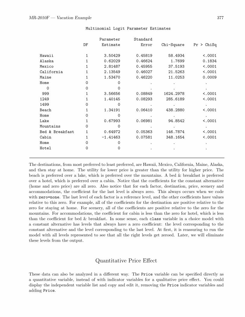
MR-2010F — Vacation Example 377
Multinomial Logit Parameter Estimates
Parameter StandardDF Estimate Error Chi-Square Pr > ChiSq
Hawaii 1 3.50429 0.45819 58.4934 <.0001Alaska 1 0.62029 0.46624 1.7699 0.1834Mexico 1 2.81487 0.45955 37.5193 <.0001California 1 2.13549 0.46027 21.5263 <.0001Maine 1 1.53470 0.46220 11.0253 0.0009Home 0 0 . . .
0 0 0 . . .999 1 3.56656 0.08849 1624.2978 <.0001
1249 1 1.40145 0.08293 285.6189 <.00011499 0 0 . . .Beach 1 1.34191 0.06410 438.2880 <.0001Home 0 0 . . .Lake 1 0.67993 0.06981 94.8542 <.0001Mountains 0 0 . . .Bed & Breakfast 1 0.64972 0.05363 146.7874 <.0001Cabin 1 -1.41463 0.07581 348.1654 <.0001Home 0 0 . . .Hotel 0 0 . . .
The destinations, from most preferred to least preferred, are Hawaii, Mexico, California, Maine, Alaska,and then stay at home. The utility for lower price is greater than the utility for higher price. Thebeach is preferred over a lake, which is preferred over the mountains. A bed & breakfast is preferredover a hotel, which is preferred over a cabin. Notice that the coefficients for the constant alternative(home and zero price) are all zero. Also notice that for each factor, destination, price, scenery andaccommodations, the coefficient for the last level is always zero. This always occurs when we codewith zero=none. The last level of each factor is a reference level, and the other coefficients have valuesrelative to this zero. For example, all of the coefficients for the destination are positive relative to thezero for staying at home. For scenery, all of the coefficients are positive relative to the zero for themountains. For accommodations, the coefficient for cabin is less than the zero for hotel, which is lessthan the coefficient for bed & breakfast. In some sense, each class variable in a choice model witha constant alternative has levels that always have a zero coefficient: the level corresponding to theconstant alternative and the level corresponding to the last level. At first, it is reassuring to run themodel with all levels represented to see that all the right levels get zeroed. Later, we will eliminatethese levels from the output.
Quantitative Price Effect
These data can also be analyzed in a different way. The Price variable can be specified directly asa quantitative variable, instead of with indicator variables for a qualitative price effect. You coulddisplay the independent variable list and copy and edit it, removing the Price indicator variables andadding Price.

378 MR-2010F — Discrete Choice
The following statement displays the list:
%put &_trgind;
Alternatively, you could run PROC TRANSREG again with the new coding. We use this latterapproach, because it is easier, and it lets us illustrate other options. In the previous analysis, thereare a number of structural zeros in the parameter estimate results due to the usage of the zero=noneoption in the PROC TRANSREG coding. This is a good thing, particularly for a first attempt atthe analysis. It is good to specify zero=none and check the results and make sure you have the rightpattern of zeros and nonzeros. Later, you can run again excluding some of the structural zeros. Thistime, we explicitly specify the ’Home’ level in the zero= option as the reference level so it is omittedfrom the & trgind variable list. The first class specification specifies zero=’Home’ since there is onevariable. The second class specification specifies zero=’Home’ ’Home’ specifying the reference levelfor each of the two variables. The variable Price is designated as an identity variable. The identitytransformation is the no-transformation option, which is used for variables that need to enter the modelwith no further manipulations. The identity variables are simply copied into the output data set andadded to the & trgind variable list. The statement label price = ’Price’ is specified to explicitlyset a label for the identity variable price. This is because we explicitly modified PROC PHREGoutput using %phchoice(on) so that the rows of the parameter estimate table are labeled only withvariable labels not variable names. A label for Price must be explicitly specified in order for the outputto contain a label for the price effect. The following steps perform the coding and the analysis:
proc transreg design data=res2 nozeroconstant norestoremissing;model class(place / zero=’Home’ order=data) identity(price)
class(scene lodge / zero=’Home’ ’Home’ order=formatted) /lprefix=0;
output out=coded(drop=_type_ _name_ intercept);label price = ’Price’;id subj set form c;run;
proc phreg data=coded brief;model c*c(2) = &_trgind / ties=breslow;strata subj set;run;
The results are as follows:
Vacation Example
The PHREG Procedure
Model Information
Data Set WORK.CODEDDependent Variable cCensoring Variable cCensoring Value(s) 2Ties Handling BRESLOW
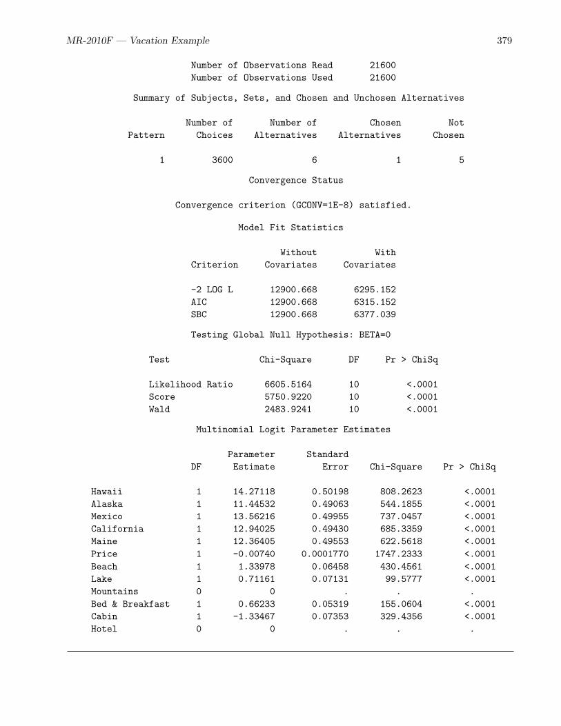
MR-2010F — Vacation Example 379
Number of Observations Read 21600Number of Observations Used 21600
Summary of Subjects, Sets, and Chosen and Unchosen Alternatives
Number of Number of Chosen NotPattern Choices Alternatives Alternatives Chosen
1 3600 6 1 5
Convergence Status
Convergence criterion (GCONV=1E-8) satisfied.
Model Fit Statistics
Without WithCriterion Covariates Covariates
-2 LOG L 12900.668 6295.152AIC 12900.668 6315.152SBC 12900.668 6377.039
Testing Global Null Hypothesis: BETA=0
Test Chi-Square DF Pr > ChiSq
Likelihood Ratio 6605.5164 10 <.0001Score 5750.9220 10 <.0001Wald 2483.9241 10 <.0001
Multinomial Logit Parameter Estimates
Parameter StandardDF Estimate Error Chi-Square Pr > ChiSq
Hawaii 1 14.27118 0.50198 808.2623 <.0001Alaska 1 11.44532 0.49063 544.1855 <.0001Mexico 1 13.56216 0.49955 737.0457 <.0001California 1 12.94025 0.49430 685.3359 <.0001Maine 1 12.36405 0.49553 622.5618 <.0001Price 1 -0.00740 0.0001770 1747.2333 <.0001Beach 1 1.33978 0.06458 430.4561 <.0001Lake 1 0.71161 0.07131 99.5777 <.0001Mountains 0 0 . . .Bed & Breakfast 1 0.66233 0.05319 155.0604 <.0001Cabin 1 -1.33467 0.07353 329.4356 <.0001Hotel 0 0 . . .

380 MR-2010F — Discrete Choice
The results of the two different analyses are similar. The coefficients for the destinations all increaseby a nonconstant amount (approximately 10.8) but the pattern is the same. There is still a negativeeffect for price. Also, the fit of this model is slightly worse, Chi-Square = 6605.5164, compared to theprevious value of 6642.9164 (bigger values mean better fit), because price has one fewer parameter.
Quadratic Price Effect
Previously, we saw price treated as a qualitative factor with two parameters and two df, then we sawprice treated as a quantitative factor with one parameter and one df. Alternatively, we could treat priceas quantitative and add a quadratic price effect (price squared). Like treating price as a qualitativefactor, there are two parameters and two df for price. First, we create PriceL, the linear price termby centering the original price and dividing by the price increment (250). This maps (999, 1249, 1499)to (−1, 0, 1). Next, we run PROC TRANSREG and PROC PHREG with the new price variables asfollows:
data res3;set res2;PriceL = price;if price then pricel = (price - 1249) / 250;run;
proc transreg design=5000 data=res3 nozeroconstant norestoremissing;model class(place / zero=’Home’ order=data)
pspline(pricel / degree=2)class(scene lodge / zero=’Home’ ’Home’ order=formatted) /lprefix=0;
output out=coded(drop=_type_ _name_ intercept);label pricel = ’Price’;id subj set form c;run;
The pspline or polynomial spline expansion with the degree=2 option replaces the variable PriceLwith two coded variables, PriceL 1 (which is the same as the original PriceL) and PriceL 2 (which isPriceL squared). A degree=2 spline with no knots (neither knots= nor nknots= is specified) simplyexpands the variable into a quadratic polynomial.
The following step fits the model:
proc phreg data=coded brief;model c*c(2) = &_trgind / ties=breslow;strata subj set;run;

MR-2010F — Vacation Example 381
This step produced the following results:
Vacation Example
The PHREG Procedure
Model Information
Data Set WORK.CODEDDependent Variable cCensoring Variable cCensoring Value(s) 2Ties Handling BRESLOW
Number of Observations Read 21600Number of Observations Used 21600
Summary of Subjects, Sets, and Chosen and Unchosen Alternatives
Number of Number of Chosen NotPattern Choices Alternatives Alternatives Chosen
1 3600 6 1 5
Convergence Status
Convergence criterion (GCONV=1E-8) satisfied.
Model Fit Statistics
Without WithCriterion Covariates Covariates
-2 LOG L 12900.668 6257.752AIC 12900.668 6279.752SBC 12900.668 6347.827
Testing Global Null Hypothesis: BETA=0
Test Chi-Square DF Pr > ChiSq
Likelihood Ratio 6642.9164 11 <.0001Score 5858.3798 11 <.0001Wald 2482.5118 11 <.0001

382 MR-2010F — Discrete Choice
Multinomial Logit Parameter Estimates
Parameter StandardDF Estimate Error Chi-Square Pr > ChiSq
Hawaii 1 4.90574 0.45379 116.8713 <.0001Alaska 1 2.02174 0.46010 19.3081 <.0001Mexico 1 4.21633 0.45427 86.1476 <.0001California 1 3.53695 0.45507 60.4085 <.0001Maine 1 2.93615 0.45761 41.1683 <.0001Price 1 1 -1.78328 0.04425 1624.2978 <.0001Price 2 1 0.38183 0.06263 37.1732 <.0001Beach 1 1.34191 0.06410 438.2880 <.0001Lake 1 0.67993 0.06981 94.8542 <.0001Mountains 0 0 . . .Bed & Breakfast 1 0.64972 0.05363 146.7874 <.0001Cabin 1 -1.41463 0.07581 348.1654 <.0001Hotel 0 0 . . .
The fit is exactly the same as when price is treated as qualitative, Chi-Square = 6642.9164. This isbecause both models are the same except for the different but equivalent 2 df codings of price. Thecoefficients for the destinations in the two models differ by a constant 1.40145. The coefficients for thefactors after price are unchanged. The part-worth utility for $999 is −1.78328 × (999 − 1249)/250 +0.38183 × ((999 − 1249)/250)2 = 2.16511, the part-worth utility for $1249 is −1.78328 × (1249 −1249)/250 + 0.38183 × ((1249 − 1249)/250)2 = 0, and the part-worth utility for $1499 is −1.78328 ×(1499−1249)/250+0.38183×((1499−1249)/250)2 = −1.40145, which differ from the coefficients whenprice is treated as qualitative, by a constant −1.40145.
Effects Coding
In the previous analyses, binary (1, 0) codings are used for the variables. The next analysis illustrateseffects (1, 0, −1) coding. The two codings differ in how the final reference level is coded. In binarycoding, the reference level is coded with zeros. In effects coding, the reference level is coded with minusones.
Binary Coding Effects Coding
Levels One Two One Two1 1 0 1 02 0 1 0 13 0 0 -1 -1
In this example, we use a binary coding for the destinations and effects codings for the attributes.
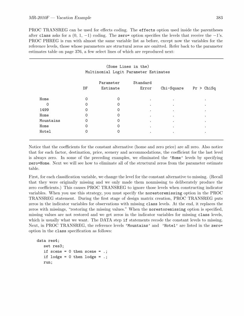
MR-2010F — Vacation Example 383
PROC TRANSREG can be used for effects coding. The effects option used inside the parenthesesafter class asks for a (0, 1, −1) coding. The zero= option specifies the levels that receive the −1’s.PROC PHREG is run with almost the same variable list as before, except now the variables for thereference levels, those whose parameters are structural zeros are omitted. Refer back to the parameterestimates table on page 376, a few select lines of which are reproduced next:
(Some Lines in the)Multinomial Logit Parameter Estimates
Parameter StandardDF Estimate Error Chi-Square Pr > ChiSq
Home 0 0 . . .0 0 0 . . .
1499 0 0 . . .Home 0 0 . . .Mountains 0 0 . . .Home 0 0 . . .Hotel 0 0 . . .
Notice that the coefficients for the constant alternative (home and zero price) are all zero. Also noticethat for each factor, destination, price, scenery and accommodations, the coefficient for the last levelis always zero. In some of the preceding examples, we eliminated the ’Home’ levels by specifyingzero=Home. Next we will see how to eliminate all of the structural zeros from the parameter estimatetable.
First, for each classification variable, we change the level for the constant alternative to missing. (Recallthat they were originally missing and we only made them nonmissing to deliberately produce thezero coefficients.) This causes PROC TRANSREG to ignore those levels when constructing indicatorvariables. When you use this strategy, you must specify the norestoremissing option in the PROCTRANSREG statement. During the first stage of design matrix creation, PROC TRANSREG putszeros in the indicator variables for observations with missing class levels. At the end, it replaces thezeros with missings, “restoring the missing values.” When the norestoremissing option is specified,missing values are not restored and we get zeros in the indicator variables for missing class levels,which is usually what we want. The DATA step if statements recode the constant levels to missing.Next, in PROC TRANSREG, the reference levels ’Mountains’ and ’Hotel’ are listed in the zero=option in the class specification as follows:
data res4;set res3;if scene = 0 then scene = .;if lodge = 0 then lodge = .;run;

384 MR-2010F — Discrete Choice
proc transreg design=5000 data=res4 nozeroconstant norestoremissing;model class(place / zero=’Home’ order=data)
pspline(pricel / degree=2)class(scene lodge /
effects zero=’Mountains’ ’Hotel’ order=formatted) /lprefix=0;
output out=coded(drop=_type_ _name_ intercept);label pricel = ’Price’;id subj set form c;run;
Next, the coded data and design matrix are displayed for the first choice set. The coded design matrixbegins with five binary columns for the destinations, ’Hawaii’ through ’Maine’. There is not a columnfor the stay-at-home destination and the row for stay at home has all zeros in the coded variables. Nextis the linear price effect, ’Price 1’, consisting of 0, 1, and −1. It is followed by the quadratic priceeffect, ’Price 2’, which is ’Price 1’ squared. Next are the scenery terms, effects coded. ’Beach’and ’Lake’ have values of 0 and 1; −1’s in the fourth row for the reference level, ’Mountains’; andzeros in the last row for the stay-at-home alternative. Next are the lodging terms, effects coded. ’Bed& Breakfast’ and ’Cabin’ have values of 0 and 1; −1’s in the first, third and fourth row for thereference level, ’Hotel’; and zeros in the last row for the stay-at-home alternative. The following stepdisplays the lodging terms:
proc print data=coded(obs=6) label; run;
The results are as follows:
Vacation Example
Price Price Bed &Obs Hawaii Alaska Mexico California Maine 1 2 Beach Lake Breakfast Cabin
1 1 0 0 0 0 -1 1 1 0 0 12 0 1 0 0 0 -1 1 -1 -1 -1 -13 0 0 1 0 0 0 0 1 0 -1 -14 0 0 0 1 0 0 0 0 1 0 15 0 0 0 0 1 0 0 -1 -1 0 16 0 0 0 0 0 0 0 0 0 0 0
Obs Place Price Scene Lodge Subj Set Form c
1 Hawaii -1 Beach Cabin 1 1 1 12 Alaska -1 Mountains Hotel 1 1 1 23 Mexico 0 Beach Hotel 1 1 1 24 California 0 Lake Cabin 1 1 1 25 Maine 0 Mountains Cabin 1 1 1 26 Home 0 . . 1 1 1 2

MR-2010F — Vacation Example 385
The following step fits the choice model:
proc phreg data=coded brief;model c*c(2) = &_trgind / ties=breslow;strata subj set;run;
The results are as follows:
Vacation Example
The PHREG Procedure
Model Information
Data Set WORK.CODEDDependent Variable cCensoring Variable cCensoring Value(s) 2Ties Handling BRESLOW
Number of Observations Read 21600Number of Observations Used 21600
Summary of Subjects, Sets, and Chosen and Unchosen Alternatives
Number of Number of Chosen NotPattern Choices Alternatives Alternatives Chosen
1 3600 6 1 5
Convergence Status
Convergence criterion (GCONV=1E-8) satisfied.
Model Fit Statistics
Without WithCriterion Covariates Covariates
-2 LOG L 12900.668 6257.752AIC 12900.668 6279.752SBC 12900.668 6347.827
Testing Global Null Hypothesis: BETA=0
Test Chi-Square DF Pr > ChiSq
Likelihood Ratio 6642.9164 11 <.0001Score 5858.3798 11 <.0001Wald 2482.5118 11 <.0001

386 MR-2010F — Discrete Choice
Multinomial Logit Parameter Estimates
Parameter StandardDF Estimate Error Chi-Square Pr > ChiSq
Hawaii 1 5.32472 0.44985 140.1076 <.0001Alaska 1 2.44072 0.45690 28.5360 <.0001Mexico 1 4.63531 0.45052 105.8613 <.0001California 1 3.95593 0.45176 76.6803 <.0001Maine 1 3.35513 0.45381 54.6610 <.0001Price 1 1 -1.78328 0.04425 1624.2978 <.0001Price 2 1 0.38183 0.06263 37.1732 <.0001Beach 1 0.66796 0.03582 347.7320 <.0001Lake 1 0.00599 0.03922 0.0233 0.8787Bed & Breakfast 1 0.90469 0.03471 679.2342 <.0001Cabin 1 -1.15966 0.04650 621.9367 <.0001
It is instructive to compare the results of this analysis to the previous analysis on page 381. First, themodel fit and chi-square statistics are the same indicating the models are equivalent. The coefficientsfor the destinations differ by a constant −0.41898, the price coefficients are the same, the scenerycoefficients differ by a constant 0.67395, and the lodging coefficients differ by a constant −0.25497.Notice that −0.41898 + 0 + 0.67395 +−0.25497 = 0, so the utility for each alternative is unchanged bythe different but equivalent codings.
Alternative-Specific Effects
In all of the analyses presented so far in this example, we have assumed that the effects for price,scenery, and accommodations are generic or constant across the different destinations. Equivalently,we assumed that destination does not interact with the attributes. Next, we show a model withalternative-specific effects that does not make this assumption. The alternative-specific model allowsfor different price, scenery and lodging effects for each destination. The coding can be done with PROCTRANSREG using its syntax for interactions. Before we do the coding, let’s go back to the designpreparation stage and redo it in a more normal fashion so reference levels are omitted from the analysis.
We start by creating the data set Key as follows:
data key;input Place $ 1-10 (Lodge Scene Price) ($);datalines;
Hawaii x1 x6 x11Alaska x2 x7 x12Mexico x3 x8 x13California x4 x9 x14Maine x5 x10 x15. . . .;

MR-2010F — Vacation Example 387
This step differs from the one we saw on page 356 only in that now we have a missing value for Placefor the constant alternative.Next, we use the %MktRoll macro to process the design and the %MktMergemacro to merge the design and data as follows:
%mktroll(design=sasuser.VacationLinDesBlckd, key=key, alt=place,out=sasuser.VacationChDes)
%mktmerge(design=sasuser.VacationChDes, data=results, out=res2, blocks=form,nsets=&n, nalts=&m, setvars=choose1-choose&n,stmts=%str(price = input(put(price, price.), 5.);
format scene scene. lodge lodge.;))
proc print data=res2(obs=12); run;
The usage of the %MktRoll macro is exactly the same as we saw on page 356. The %MktMerge macrousage differs from page 371 in that instead of assigning labels and recoding price in a separate DATAstep, we now do it directly in the macro. The stmts= option is used to add a price = assignmentstatement and format statement to the DATA step that merges the two data sets. The statements areincluded in a %str( ) macro since they contain semicolons. The first two choice sets are as follows:
Vacation Example
Obs Subj Form Set Place Lodge Scene Price c
1 1 1 1 Hawaii Cabin Beach 999 12 1 1 1 Alaska Hotel Mountains 999 23 1 1 1 Mexico Hotel Beach 1249 24 1 1 1 California Cabin Lake 1249 25 1 1 1 Maine Cabin Mountains 1249 26 1 1 1 . . . 27 1 1 2 Hawaii Cabin Beach 999 18 1 1 2 Alaska Bed & Breakfast Lake 1499 29 1 1 2 Mexico Cabin Lake 999 210 1 1 2 California Bed & Breakfast Mountains 999 211 1 1 2 Maine Hotel Beach 1249 212 1 1 2 . . . 2
Notice that the attributes for the constant alternative are all missing. Next, we code with PROCTRANSREG. Since we are using missing values for the constant alternative, we must specify thenorestoremissing option in the PROC TRANSREG statement. With the norestoremissing option,the indicator variables created for missing class variable values contain all zeros instead of all missings.First, we specify the variable Place as a class variable.
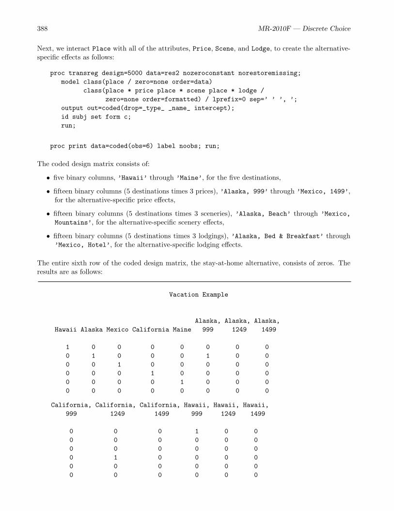
388 MR-2010F — Discrete Choice
Next, we interact Place with all of the attributes, Price, Scene, and Lodge, to create the alternative-specific effects as follows:
proc transreg design=5000 data=res2 nozeroconstant norestoremissing;model class(place / zero=none order=data)
class(place * price place * scene place * lodge /zero=none order=formatted) / lprefix=0 sep=’ ’ ’, ’;
output out=coded(drop=_type_ _name_ intercept);id subj set form c;run;
proc print data=coded(obs=6) label noobs; run;
The coded design matrix consists of:
• five binary columns, ’Hawaii’ through ’Maine’, for the five destinations,
• fifteen binary columns (5 destinations times 3 prices), ’Alaska, 999’ through ’Mexico, 1499’,for the alternative-specific price effects,
• fifteen binary columns (5 destinations times 3 sceneries), ’Alaska, Beach’ through ’Mexico,Mountains’, for the alternative-specific scenery effects,
• fifteen binary columns (5 destinations times 3 lodgings), ’Alaska, Bed & Breakfast’ through’Mexico, Hotel’, for the alternative-specific lodging effects.
The entire sixth row of the coded design matrix, the stay-at-home alternative, consists of zeros. Theresults are as follows:
Vacation Example
Alaska, Alaska, Alaska,Hawaii Alaska Mexico California Maine 999 1249 1499
1 0 0 0 0 0 0 00 1 0 0 0 1 0 00 0 1 0 0 0 0 00 0 0 1 0 0 0 00 0 0 0 1 0 0 00 0 0 0 0 0 0 0
California, California, California, Hawaii, Hawaii, Hawaii,999 1249 1499 999 1249 1499
0 0 0 1 0 00 0 0 0 0 00 0 0 0 0 00 1 0 0 0 00 0 0 0 0 00 0 0 0 0 0

MR-2010F — Vacation Example 389
Maine, Maine, Maine, Mexico, Mexico, Mexico, Alaska, Alaska, Alaska,999 1249 1499 999 1249 1499 Beach Lake Mountains
0 0 0 0 0 0 0 0 00 0 0 0 0 0 0 0 10 0 0 0 1 0 0 0 00 0 0 0 0 0 0 0 00 1 0 0 0 0 0 0 00 0 0 0 0 0 0 0 0
California, California, California, Hawaii, Hawaii, Hawaii,Beach Lake Mountains Beach Lake Mountains
0 0 0 1 0 00 0 0 0 0 00 0 0 0 0 00 1 0 0 0 00 0 0 0 0 00 0 0 0 0 0
Alaska,Maine, Maine, Maine, Mexico, Mexico, Mexico, Bed & Alaska, Alaska,Beach Lake Mountains Beach Lake Mountains Breakfast Cabin Hotel
0 0 0 0 0 0 0 0 00 0 0 0 0 0 0 0 10 0 0 1 0 0 0 0 00 0 0 0 0 0 0 0 00 0 1 0 0 0 0 0 00 0 0 0 0 0 0 0 0
California, Hawaii,Bed & California, California, Bed & Hawaii, Hawaii,
Breakfast Cabin Hotel Breakfast Cabin Hotel
0 0 0 0 1 00 0 0 0 0 00 0 0 0 0 00 1 0 0 0 00 0 0 0 0 00 0 0 0 0 0

390 MR-2010F — Discrete Choice
Maine, Mexico,Bed & Maine, Maine, Bed & Mexico, Mexico,Breakfast Cabin Hotel Breakfast Cabin Hotel Place
0 0 0 0 0 0 Hawaii0 0 0 0 0 0 Alaska0 0 0 0 0 1 Mexico0 0 0 0 0 0 California0 1 0 0 0 0 Maine0 0 0 0 0 0
Price Scene Lodge Subj Set Form c
999 Beach Cabin 1 1 1 1999 Mountains Hotel 1 1 1 21249 Beach Hotel 1 1 1 21249 Lake Cabin 1 1 1 21249 Mountains Cabin 1 1 1 2
. . . 1 1 1 2
Analysis proceeds by running PROC PHREG as follows:
proc phreg data=coded brief;model c*c(2) = &_trgind / ties=breslow;strata subj set;run;
The results are as follows:
Vacation Example
The PHREG Procedure
Model Information
Data Set WORK.CODEDDependent Variable cCensoring Variable cCensoring Value(s) 2Ties Handling BRESLOW
Number of Observations Read 21600Number of Observations Used 21600

MR-2010F — Vacation Example 391
Summary of Subjects, Sets, and Chosen and Unchosen Alternatives
Number of Number of Chosen NotPattern Choices Alternatives Alternatives Chosen
1 3600 6 1 5
Convergence Status
Convergence criterion (GCONV=1E-8) satisfied.
Model Fit Statistics
Without WithCriterion Covariates Covariates
-2 LOG L 12900.668 6239.870AIC 12900.668 6309.870SBC 12900.668 6526.474
Testing Global Null Hypothesis: BETA=0
Test Chi-Square DF Pr > ChiSq
Likelihood Ratio 6660.7982 35 <.0001Score 6601.7928 35 <.0001Wald 2448.1475 35 <.0001
Multinomial Logit Parameter Estimates
Parameter StandardDF Estimate Error Chi-Square Pr > ChiSq
Hawaii 1 3.49208 0.47222 54.6856 <.0001Alaska 1 0.17527 0.67139 0.0682 0.7940Mexico 1 2.93013 0.47932 37.3706 <.0001California 1 2.17915 0.49725 19.2058 <.0001Maine 1 1.27770 0.54587 5.4787 0.0192Alaska, 999 1 4.02423 0.46534 74.7858 <.0001Alaska, 1249 1 1.81200 0.49473 13.4147 0.0002Alaska, 1499 0 0 . . .
California, 999 1 3.38438 0.19965 287.3498 <.0001California, 1249 1 1.22372 0.22445 29.7251 <.0001California, 1499 0 0 . . .
Hawaii, 999 1 3.61016 0.14157 650.2879 <.0001Hawaii, 1249 1 1.45415 0.13050 124.1725 <.0001Hawaii, 1499 0 0 . . .
Maine, 999 1 3.80918 0.26060 213.6577 <.0001Maine, 1249 1 1.53370 0.27050 32.1475 <.0001Maine, 1499 0 0 . . .

392 MR-2010F — Discrete Choice
Mexico, 999 1 3.45924 0.15495 498.4209 <.0001Mexico, 1249 1 1.41406 0.15693 81.1907 <.0001Mexico, 1499 0 0 . . .
Alaska, Beach 1 1.01542 0.21881 21.5355 <.0001Alaska, Lake 1 0.48168 0.22639 4.5269 0.0334Alaska, Mountains 0 0 . . .
California, Beach 1 1.47681 0.15536 90.3528 <.0001California, Lake 1 0.84358 0.16138 27.3244 <.0001California, Mountains 0 0 . . .
Hawaii, Beach 1 1.29573 0.12493 107.5692 <.0001Hawaii, Lake 1 0.61301 0.12299 24.8444 <.0001Hawaii, Mountains 0 0 . . .
Maine, Beach 1 1.59739 0.20874 58.5584 <.0001Maine, Lake 1 0.64984 0.20203 10.3468 0.0013Maine, Mountains 0 0 . . .
Mexico, Beach 1 1.26780 0.13744 85.0857 <.0001Mexico, Lake 1 0.67632 0.13589 24.7716 <.0001Mexico, Mountains 0 0 . . .
Alaska, Bed & Breakfast 1 1.00195 0.18862 28.2169 <.0001Alaska, Cabin 1 -1.33747 0.31958 17.5146 <.0001Alaska, Hotel 0 0 . . .
California, Bed & Breakfast 1 0.67004 0.13195 25.7875 <.0001California, Cabin 1 -1.50239 0.16734 80.6060 <.0001California, Hotel 0 0 . . .
Hawaii, Bed & Breakfast 1 0.63585 0.11523 30.4508 <.0001Hawaii, Cabin 1 -1.41004 0.13462 109.7155 <.0001Hawaii, Hotel 0 0 . . .
Maine, Bed & Breakfast 1 0.58532 0.15999 13.3848 0.0003Maine, Cabin 1 -1.50967 0.22377 45.5166 <.0001Maine, Hotel 0 0 . . .
Mexico, Bed & Breakfast 1 0.54835 0.11802 21.5891 <.0001Mexico, Cabin 1 -1.40762 0.15033 87.6707 <.0001Mexico, Hotel 0 0 . . .
There are zero coefficients for the reference level. Do we need this more complicated model insteadof the simpler model? To answer this, first look at the coefficients. Are they similar across differentdestinations? In this case, they seem to be. This suggests that the simpler model might be sufficient.
More formally, the two models can be statistically compared. You can test the null hypothesis that thetwo models are not significantly different by comparing their likelihoods. The difference between two−2 log(LC)’s (the number reported under ’With Covariates’ in the output) has a chi-square distribution.We can get the df for the test by subtracting the two df for the two likelihoods. The difference6257.752 − 6239.870 = 17.882 is distributed χ2 with 35 − 11 = 24 df (p < 0.80869). This morecomplicated model does not account for significantly more variance than the simpler model.

MR-2010F — Vacation Example and Artificial Data Generation 393
Vacation Example and Artificial DataGeneration
This example does not illustrate any new capabilities. Rather, it shows how to make artificial data totest your design and your code for processing and analyzing the real data before the data are collected.This example goes into more detail about how to create artificial data than the other artificial dataexamples in this chapter. The artificial data creation step assumes that the design is in the final choicedesign format (not in the linear arrangement that comes from the %MktEx macro).
You begin by making a design. This example is based on the vacation example on page 339. The goalis to make an alternative-specific design for vacation destinations. The choice design has a destinationattribute along with three other attributes, accommodations, scenery, and price. The design can beconstructed from a linear arrangement with the following factors:
Factor Destination Attribute Levels
X1 Hawaii Accommodations Cabin, Bed & Breakfast, HotelX2 Alaska Accommodations Cabin, Bed & Breakfast, HotelX3 Mexico Accommodations Cabin, Bed & Breakfast, HotelX4 California Accommodations Cabin, Bed & Breakfast, HotelX5 Maine Accommodations Cabin, Bed & Breakfast, Hotel
X6 Hawaii Scenery Mountains, Lake, BeachX7 Alaska Scenery Mountains, Lake, BeachX8 Mexico Scenery Mountains, Lake, BeachX9 California Scenery Mountains, Lake, BeachX10 Maine Scenery Mountains, Lake, Beach
X11 Hawaii Price $999, $1249, $1499X12 Alaska Price $999, $1249, $1499X13 Mexico Price $999, $1249, $1499X14 California Price $999, $1249, $1499X15 Maine Price $999, $1249, $1499
The design additionally has a constant “stay at home” alternative.
The %MktEx macro can be used as follows to make a linear arrangement in 36 runs, which becomes achoice design with 36 choice sets:
%mktex(3 ** 15, /* 15 three-level factors */n=36, /* 36 rows in linear arrang - 36 ch sets*/seed=205) /* random number seed */
The linear arrangement is blocked into two blocks of size 18 as follows:
%mktblock(data=randomized, /* block randomized design */nblocks=2, /* create two blocks of 18 choice sets */out=blocked, /* output data set for blocked design */seed=114) /* random number seed */
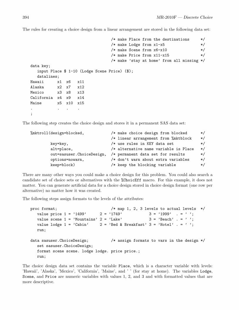
394 MR-2010F — Discrete Choice
The rules for creating a choice design from a linear arrangement are stored in the following data set:
/* make Place from the destinations *//* make Lodge from x1-x5 *//* make Scene from x6-x10 *//* make Price from x11-x15 *//* make ’stay at home’ from all missing */
data key;input Place $ 1-10 (Lodge Scene Price) ($);datalines;
Hawaii x1 x6 x11Alaska x2 x7 x12Mexico x3 x8 x13California x4 x9 x14Maine x5 x10 x15. . . .;
The following step creates the choice design and stores it in a permanent SAS data set:
%mktroll(design=blocked, /* make choice design from blocked *//* linear arrangement from %mktblock */
key=key, /* use rules in KEY data set */alt=place, /* alternative name variable is Place */out=sasuser.ChoiceDesign, /* permanent data set for results */options=nowarn, /* don’t warn about extra variables */keep=block) /* keep the blocking variable */
There are many other ways you could make a choice design for this problem. You could also search acandidate set of choice sets or alternatives with the %ChoicEff macro. For this example, it does notmatter. You can generate artificial data for a choice design stored in choice design format (one row peralternative) no matter how it was created.
The following steps assign formats to the levels of the attributes:
proc format; /* map 1, 2, 3 levels to actual levels */value price 1 = ’1499’ 2 = ’1749’ 3 = ’1999’ . = ’ ’;value scene 1 = ’Mountains’ 2 = ’Lake’ 3 = ’Beach’ . = ’ ’;value lodge 1 = ’Cabin’ 2 = ’Bed & Breakfast’ 3 = ’Hotel’ . = ’ ’;run;
data sasuser.ChoiceDesign; /* assign formats to vars in the design */set sasuser.ChoiceDesign;format scene scene. lodge lodge. price price.;run;
The choice design data set contains the variable Place, which is a character variable with levels:’Hawaii’, ’Alaska’, ’Mexico’, ’California’, ’Maine’, and ’ ’ (for stay at home). The variables Lodge,Scene, and Price are numeric variables with values 1, 2, and 3 and with formatted values that aremore descriptive.

MR-2010F — Vacation Example and Artificial Data Generation 395
The following step displays the choice design:
proc print data=sasuser.ChoiceDesign; /* display sets and check results */by block set; id block set;run;
It is important to display the choice design and ensure that it is correct. Some of the results are asfollows:
Block Set Place Lodge Scene Price
1 1 Hawaii Cabin Beach 1999Alaska Hotel Lake 1999Mexico Cabin Lake 1499California Cabin Lake 1749Maine Hotel Beach 1999
1 2 Hawaii Cabin Mountains 1499Alaska Bed & Breakfast Mountains 1999Mexico Bed & Breakfast Mountains 1999California Hotel Lake 1749Maine Hotel Mountains 1749
.
.
.
1 18 Hawaii Bed & Breakfast Lake 1999Alaska Hotel Beach 1749Mexico Cabin Lake 1999California Bed & Breakfast Beach 1749Maine Cabin Lake 1749
.
.
.
2 36 Hawaii Bed & Breakfast Lake 1499Alaska Bed & Breakfast Lake 1999Mexico Hotel Mountains 1749California Cabin Beach 1499Maine Cabin Beach 1999

396 MR-2010F — Discrete Choice
The following step evaluates the choice design by using the %ChoicEff macro:
/* Evaluate the choice design */%choiceff(data=sasuser.ChoiceDesign,/* candidate set of choice sets */
init=sasuser.ChoiceDesign(keep=set), /* select these sets */intiter=0, /* evaluate without internal iterations */
/* alternative-specific effects model *//* zero=none - no ref levels for place *//* order=data - do not sort levels */
model=class(place / zero=none order=data)/* zero=’ ’ - no ref level for first *//* factor (place), ordinary ref levels *//* for other factors (price -- lodge). *//* order=formatted - sort levels *//* use blank sep to build interact terms*/
class(place * price place * scene place * lodge /zero=’ ’ order=formatted separators=’’ ’ ’) /
/* no ref level for place *//* use blank sep to build interact terms*/
lprefix=0 /* lpr=0 labels created from just levels*/cprefix=0, /* cpr=0 names created from just levels */
nsets=72, /* number of choice sets */nalts=6, /* number of alternatives */beta=zero) /* assumed beta vector, Ho: b=0 */
The list of parameters, variances, and standard errors are as follows:
Standardn Variable Name Label Variance DF Error
1 Hawaii Hawaii 0.76667 1 0.875602 Alaska Alaska 0.76667 1 0.875603 Mexico Mexico 0.76717 1 0.875884 California California 0.86667 1 0.930955 Maine Maine 0.76717 1 0.875886 Alaska_1499 Alaska 1499 0.60000 1 0.774607 Alaska_1749 Alaska 1749 0.60000 1 0.774608 California_1499 California 1499 0.80000 1 0.894439 California_1749 California 1749 0.60000 1 0.7746010 Hawaii_1499 Hawaii 1499 0.60000 1 0.7746011 Hawaii_1749 Hawaii 1749 0.60000 1 0.7746012 Maine_1499 Maine 1499 0.60150 1 0.7755713 Maine_1749 Maine 1749 0.60150 1 0.7755714 Mexico_1499 Mexico 1499 0.60150 1 0.7755715 Mexico_1749 Mexico 1749 0.60150 1 0.7755716 AlaskaBeach Alaska Beach 0.60000 1 0.7746017 AlaskaLake Alaska Lake 0.60000 1 0.7746018 CaliforniaBeach California Beach 0.60000 1 0.7746019 CaliforniaLake California Lake 0.60000 1 0.77460

MR-2010F — Vacation Example and Artificial Data Generation 397
20 HawaiiBeach Hawaii Beach 0.60000 1 0.7746021 HawaiiLake Hawaii Lake 0.60000 1 0.7746022 MaineBeach Maine Beach 0.60000 1 0.7746023 MaineLake Maine Lake 0.60000 1 0.7746024 MexicoBeach Mexico Beach 0.60000 1 0.7746025 MexicoLake Mexico Lake 0.60000 1 0.7746026 AlaskaBed___Breakfast Alaska Bed & Breakfast 0.60000 1 0.7746027 AlaskaCabin Alaska Cabin 0.60000 1 0.7746028 CaliforniaBed___Breakfast California Bed & Breakfast 0.60000 1 0.7746029 CaliforniaCabin California Cabin 0.60000 1 0.7746030 HawaiiBed___Breakfast Hawaii Bed & Breakfast 0.60000 1 0.7746031 HawaiiCabin Hawaii Cabin 0.60000 1 0.7746032 MaineBed___Breakfast Maine Bed & Breakfast 0.60000 1 0.7746033 MaineCabin Maine Cabin 0.60000 1 0.7746034 MexicoBed___Breakfast Mexico Bed & Breakfast 0.60000 1 0.7746035 MexicoCabin Mexico Cabin 0.60000 1 0.77460
==35
The next step, now that the choice design has been constructed and evaluated with the %ChoicEffmacro, is making artificial data for some fictitious subjects. Before you do that, however, you shouldstudy the next three examples which explain some of the inner workings of the SAS DATA step. Thisbackground makes the data generation program clearer. The first program is a standard DATA stepthat creates a copy of the choice design. It is not a model for what you will do. Rather, it provides astandard and familiar DATA step program, which you can compare to what you will actually do. Thefollowing step creates a copy of a data set:
data Test; /* Make one copy of the input SAS data set. *//* DATA step does automatic looping, it automatically *//* writes out the observation to a SAS data set, and it *//* automatically stops when it hits the end of file on *//* the input SAS data set. With 216 observations in *//* the input SAS data set, there are 216 passes through *//* the DATA step, and since there is no OUTPUT *//* statement, each observation is automatically written *//* to the output SAS data set by an implicit OUTPUT. */
set sasuser.ChoiceDesign;run;
In the preceding step, SAS does most of the work for you. You can use this type of DATA step whenthere is a one to one correspondence between the input and the output. The DATA step that makesthe artificial data does not have this one to one correspondence.

398 MR-2010F — Discrete Choice
The following step creates a copy of the design data set, but this time, you must program all of thelooping yourself:
data Test; /* Make one copy of the input SAS data set. There is *//* one pass through this DATA step, and the DO loop *//* reads 216 observations from the input SAS data set. */
/* Do the looping yourself. */do i = 1 to 216; /* 36 choice sets and 6 alternatives = 216 observations */
/* SET statement with POINT=i reads the ith *//* observation, and the variable i is automatically *//* dropped from the output SAS data set. */
set sasuser.ChoiceDesign point=i;
output; /* Write out each observation to a SAS data set. *//* Without this statement, an OUTPUT statement *//* implicitly appears at the end of the DATA step, *//* which would have written out only the last *//* observation if the STOP statement hadn’t stopped the *//* DATA step first. */
end;
stop; /* Must specify STOP since it never hits the end of the *//* data file (it never attempts to read past the last *//* record). Infinite loop without this statement. */
run;
This step uses one pass through the DATA step with 216 reads of the input data set. The previousstep uses 216 passes through the DATA step to perform 216 reads of the input data set. You can use avariation on this looping approach to create two copies of the output data set. Now there is no longera one-to-one correspondence between the input data set and the output data set. The following stepmakes two copies of the input data set:
data Test; /* Make two copies of the input SAS data set. *//* There is one pass through this DATA step, the outer *//* DO loop creates two copies, and the inner DO loop *//* reads 216 observations from the input SAS data set *//* (twice due to the outer DO loop). */
do Subject = 1 to 2;/* Two copies. */
/* Do the looping yourself. */do i = 1 to 216; /* 36 choice sets and 6 alternatives = 216 obs */
/* SET statement reads the ith observation, and the *//* variable i is automatically dropped from the output *//* SAS data set. */
set sasuser.ChoiceDesign point=i;
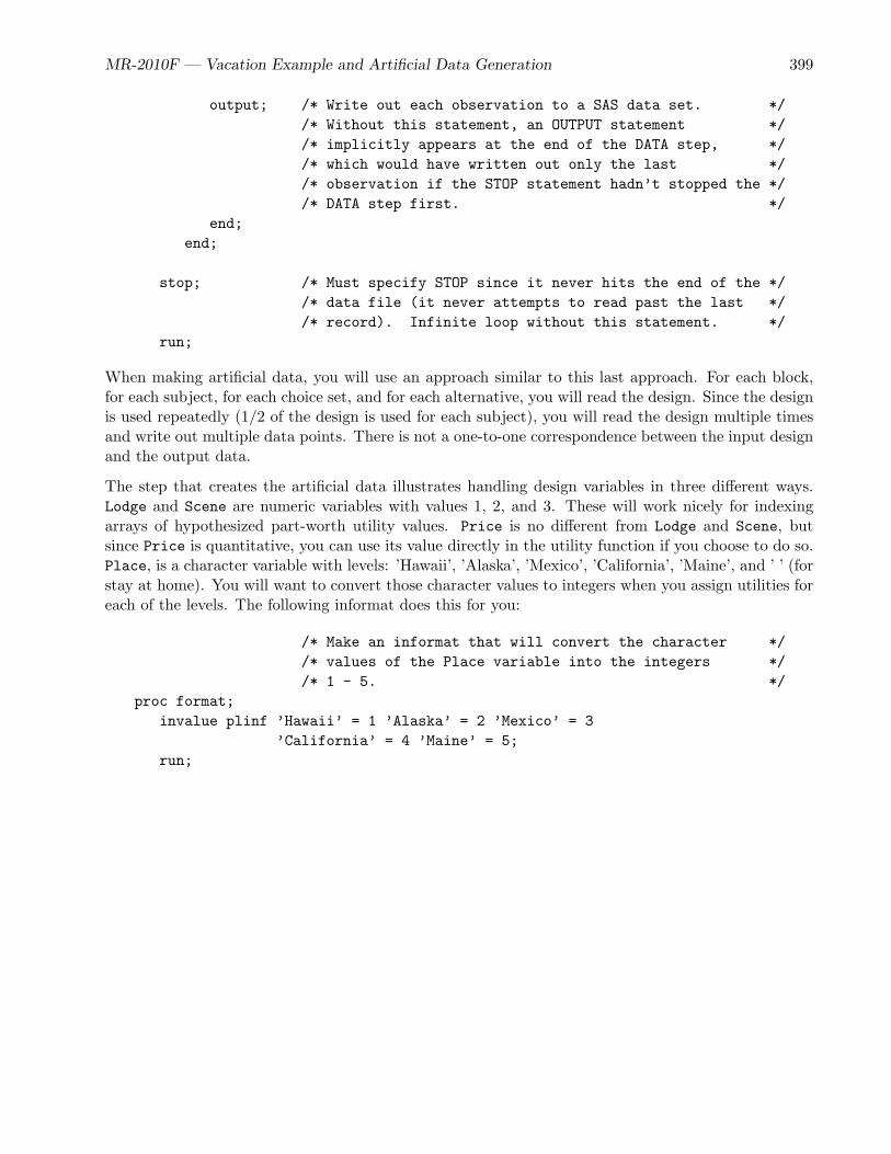
MR-2010F — Vacation Example and Artificial Data Generation 399
output; /* Write out each observation to a SAS data set. *//* Without this statement, an OUTPUT statement *//* implicitly appears at the end of the DATA step, *//* which would have written out only the last *//* observation if the STOP statement hadn’t stopped the *//* DATA step first. */
end;end;
stop; /* Must specify STOP since it never hits the end of the *//* data file (it never attempts to read past the last *//* record). Infinite loop without this statement. */
run;
When making artificial data, you will use an approach similar to this last approach. For each block,for each subject, for each choice set, and for each alternative, you will read the design. Since the designis used repeatedly (1/2 of the design is used for each subject), you will read the design multiple timesand write out multiple data points. There is not a one-to-one correspondence between the input designand the output data.
The step that creates the artificial data illustrates handling design variables in three different ways.Lodge and Scene are numeric variables with values 1, 2, and 3. These will work nicely for indexingarrays of hypothesized part-worth utility values. Price is no different from Lodge and Scene, butsince Price is quantitative, you can use its value directly in the utility function if you choose to do so.Place, is a character variable with levels: ’Hawaii’, ’Alaska’, ’Mexico’, ’California’, ’Maine’, and ’ ’ (forstay at home). You will want to convert those character values to integers when you assign utilities foreach of the levels. The following informat does this for you:
/* Make an informat that will convert the character *//* values of the Place variable into the integers *//* 1 - 5. */
proc format;invalue plinf ’Hawaii’ = 1 ’Alaska’ = 2 ’Mexico’ = 3
’California’ = 4 ’Maine’ = 5;run;

400 MR-2010F — Discrete Choice
The following step creates artificial data:
data _null_;/* DATA _NULL_ allows you to use the DATA step without creating an *//* output SAS data set. The result is a list of artificial data written *//* to the SAS log. *//* *//* Specify a list of expected utilities for each level of each *//* attribute in an array for each attribute. Recall that the Price, *//* Scene, and Lodge have actual values 1, 2, 3 that correspond to the *//* formatted values shown here: *//* *//* value price 1 = ’1499’ 2 = ’1749’ 3 = ’1999’ *//* value scene 1 = ’Mountains’ 2 = ’Lake’ 3 = ’Beach’ *//* value lodge 1 = ’Cabin’ 2 = ’Bed & Breakfast’ 3 = ’Hotel’ *//* *//* In the design data set, actual values are stored not the formatted *//* values. However, Place has only actual values. *//* *//* When Place = ’Hawaii’, *//* input(place, plinf.) = 1, and the utility, dests[1] = 5; *//* when Place = ’Alaska’, *//* input(place, plinf.) = 2, and the utility, dests[2] = -1; *//* and so on. *//* *//* When Scene = 1, and the formatted value is ’Mountains’, *//* scenes[1] = -1; and so on. *//* *//* Price has values 1 to 3 and they can be used directly in the *//* utility function (or in a way similar to the other attributes). *//* *//* _temporary_ is used when the goal is for an array name and an *//* index to access a list of values, and no data set variables are *//* created or needed. *//* *//* Be careful that your array names and variable names do not *//* conflict with variable names in the input design data set. */
array dests[5] _temporary_ (5 -1 4 3 2);array scenes[3] _temporary_ (-1 0 1);array lodging[3] _temporary_ (0 3 2);
array u[6]; /* An array to store the utility of each alt */
Subject = 0; /* Subject number */
do s = 1 to 100; /* Create data for 100 subjects per block */
i = 0; /* Observation number in the design data set */do BlockNum = 1 to 2; /* Create data for 2 blocks of 100 subjects */
Subject + 1; /* Subject number */

MR-2010F — Vacation Example and Artificial Data Generation 401
/* put / - go to a new line *//* blocknum 3. - write the block number in 3 columns *//* +2 - skip two columns *//* subject 3. - write the subject number in 3 columns *//* +2 - skip two columns *//* @@; - hold the output line for the data yet to come */put / blocknum 3. +2 subject 3. +2 @@;
do SetNum = 1 to 18; /* Loop over the 18 sets in a block */do Alt = 1 to 6; /* Loop over the 6 alts in a set */
i + 1; /* same as i = i + 1; design index, *//* i = 1 to 216 (2 blocks x 18 sets x 6 alts) */
/* Read the ith observation of the choice *//* design. Note that you are reading the *//* choice design not the linear arrangement. *//* Just read in the variables that you need. */
set sasuser.ChoiceDesign(keep=place--price) point=i;
if place ne ’ ’/* process the destinations differently */then do; /* from the constant ’stay at home’ */p = input(place, plinf.); /* map place values to 1-5 */u[alt] = 1 + /* add 1 just for not at home */
dests[p] + /* util for destination */scenes[scene] + /* util for scenery */lodging[lodge] - /* util for lodging */price; /* negative util for price */
if place = ’Hawaii’ and /* add in Hawaii/Beach */scene = 3 then /* interaction */u[alt] = u[alt] + 2;
if place = ’Maine’ and /* add Maine on a lake in a */scene = 2 and lodge = 1/* cabin interaction */then u[alt] = u[alt] + 1;
end;
else u[alt] = 0; /* util for stay at home */
u[alt] = u[alt] + 3 * normal(17); /* add error to utils *//* change ’3’ to change *//* the magnitude of error */
/* Alternatively, you can create Type I Gumbel errors for *//* some scaling parameter b as follows: *//* u[alt] = u[alt] + b * log(-log(1 - uniform(104))); */end;

402 MR-2010F — Discrete Choice
/* at this point you have gathered u1-u6 for all 6 alts */m = max(of u1-u6); /* max util over alts */
/* which one had the maximum util? do fuzzy comparison */if abs(u1 - m) < 1e-4 then c = 1; /* alt 1 is chosen */else if abs(u2 - m) < 1e-4 then c = 2; /* alt 2 is chosen */else if abs(u3 - m) < 1e-4 then c = 3; /* alt 3 is chosen */else if abs(u4 - m) < 1e-4 then c = 4; /* alt 4 is chosen */else if abs(u5 - m) < 1e-4 then c = 5; /* alt 5 is chosen */else c = 6; /* alt 6 is chosen (home)*/
put +(-1) c @@; /* write number of chosen alt. Use ’@@’ to hold *//* the line for the rest of the data in this *//* block for this subject. *//* +(-1) skips forward -1 space, which is how *//* you move back one space */
end;end;
end;stop; /* explicitly stop since no end of file is hit */run;
You can copy and paste the results, which are displayed in the SAS log file, into the following DATAstep† to input the results as you might do so when it comes time to analyze the data:
data results; /* Read the input data. List input for block *//* and subject. Formatted input (fields of *//* size 1) for choices. */
input Block Subject (choose1-choose18) (1.);datalines;1 1 4164342134153115352 2 1154115414514411511 3 1324553314341131442 4 3133132441213113141 5 4511435325414112142 6 311131311414411511...1 197 3313353331143131122 198 1113142515212111411 199 1513512111143111312 200 311314311151143141
;
†Alternatively, you could use a FILE statement in the preceding DATA step to write the data to a file (for example,FILE ’mytestdata.dat’; after the ARRAY statements). Then you could use INFILE ’mytestdata.dat’; before the INPUTstatement instead of DATALINES and in stream data after the INPUT statement. If you do this, you must ensure thatyou do not rerun this program after the data are collected and wipe out the data.

MR-2010F — Vacation Example and Artificial Data Generation 403
It is important to display the contents of the results data set to ensure that you read the input datacorrectly. The following step displays the data set:
proc print; run; /* make sure data match input */
Some of the results are as follows:
c c c c c c c c cS c c c c c c c c c h h h h h h h h hu h h h h h h h h h o o o o o o o o o
B b o o o o o o o o o o o o o o o o o ol j o o o o o o o o o s s s s s s s s s
O o e s s s s s s s s s e e e e e e e e eb c c e e e e e e e e e 1 1 1 1 1 1 1 1 1s k t 1 2 3 4 5 6 7 8 9 0 1 2 3 4 5 6 7 8
1 1 1 4 1 6 4 3 4 2 1 3 4 1 5 3 1 1 5 3 52 2 2 1 1 5 4 1 1 5 4 1 4 5 1 4 4 1 1 5 13 1 3 1 3 2 4 5 5 3 3 1 4 3 4 1 1 3 1 4 44 2 4 3 1 3 3 1 3 2 4 4 1 2 1 3 1 1 3 1 45 1 5 4 5 1 1 4 3 5 3 2 5 4 1 4 1 1 2 1 46 2 6 3 1 1 1 3 1 3 1 1 4 1 4 4 1 1 5 1 1...
199 1 199 1 5 1 3 5 1 2 1 1 1 1 4 3 1 1 1 3 1200 2 200 3 1 1 3 1 4 3 1 1 1 5 1 1 4 3 1 4 1
You should ensure that there are no unexpected missing values and that the right number of observa-tions (in this case, 2 blocks times 100 subjects) are present.
The following step merges the data and the choice design:
%mktmerge(design=sasuser.ChoiceDesign, /* merge the design data set */data=results, /* with the results */out=res2, /* create output data set res2 */blocks=block, /* name of blocking variable */nsets=18, /* number of choice sets per block */nalts=6, /* number of alternatives */setvars=choose1-choose18) /* variables with the choices */
The following step displays part of the resulting data set:
proc print data=res2(obs=18); /* display some data - sanity check */id block subject set;by block subject set;run;

404 MR-2010F — Discrete Choice
It is again important to look at the results before proceeding. The results are as follows:
Block Subject Set Place Lodge Scene Price c
1 1 1 Hawaii Cabin Beach 1999 2Alaska Hotel Lake 1999 2Mexico Cabin Lake 1499 2California Cabin Lake 1749 1Maine Hotel Beach 1999 2
2
1 1 2 Hawaii Cabin Mountains 1499 1Alaska Bed & Breakfast Mountains 1999 2Mexico Bed & Breakfast Mountains 1999 2California Hotel Lake 1749 2Maine Hotel Mountains 1749 2
2
1 1 3 Hawaii Hotel Beach 1749 2Alaska Bed & Breakfast Beach 1749 2Mexico Cabin Mountains 1499 2California Cabin Beach 1499 2Maine Hotel Mountains 1499 2
1
The following step codes the attributes for analysis:
proc transreg /* use proc transreg to code */data=res2 /* name of data set to code */design=5000 /* code big designs in chunks */
/* code up to 5000 obs at a time */nozeroconstant /* don’t zero constant variables */norestoremissing; /* zeros in coded vars, not missings */
model class(place / /* code Place variable */zero=none /* use all nonmissing levels */order=data) /* don’t sort levels */
class(place * price /* code other vars */place * sceneplace * lodge /zero=none /* use all nonmissing levels */
/* including 0 reference levels */order=formatted /* do sort levels by formatted values*/separators=’’ ’ ’) / /* use blank separator in interacts */
lprefix=0; /* make labels just from levels */output out=coded /* output coded data set */
(drop=_type_ _name_ intercept);/* drop vars that you don’t need */id subject set block c; /* add extra vars that you do need */run;
MR-2010F — Vacation Example and Artificial Data Generation 405
The following step customizes the output from PROC PHREG for choice modeling:
%phchoice( on ) /* customize output from PHREG for *//* choice models */
The following step analyzes the artificial data:
proc phreg data=coded brief; /* do analysis with a brief summary *//* of strata (set, subject, block) */
model c*c(2) = &_trgind / ties=breslow; /* standard choice model */strata subject set block; /* ID variables who taken together */run; /* identify each individual choice */
/* set */
Some of the results are as follows:
Summary of Subjects, Sets, and Chosen and Unchosen Alternatives
Number of Number of Chosen NotPattern Choices Alternatives Alternatives Chosen
1 3600 6 1 5
It is important to note that there were 3600 choices (36 choice sets and 100 subjects per set). Eachset consists of 6 alternatives—one was chosen and five were not. Each of the 3600 subject and setcombinations jointly defines a separate stratum in the analysis. Any other pattern of results for thisdesign and data set indicates an error in data collection, entry, or processing. More is said about thistable at the end of this example.
The parameter estimates are as follows:
Multinomial Logit Parameter Estimates
Parameter StandardDF Estimate Error Chi-Square Pr > ChiSq
Hawaii 1 2.29050 0.17219 176.9392 <.0001Alaska 1 -1.58858 0.49315 10.3766 0.0013Mexico 1 1.87521 0.18389 103.9896 <.0001California 1 1.32370 0.21482 37.9705 <.0001Maine 1 0.77912 0.23117 11.3595 0.0008Alaska 1499 1 1.64559 0.42064 15.3050 <.0001Alaska 1749 1 0.65152 0.44333 2.1597 0.1417Alaska 1999 0 0 . . .California 1499 1 0.97060 0.14844 42.7531 <.0001California 1749 1 0.50921 0.13822 13.5731 0.0002California 1999 0 0 . . .

406 MR-2010F — Discrete Choice
Hawaii 1499 1 0.98873 0.09483 108.7181 <.0001Hawaii 1749 1 0.49605 0.09585 26.7826 <.0001Hawaii 1999 0 0 . . .Maine 1499 1 1.19476 0.15276 61.1707 <.0001Maine 1749 1 0.74813 0.16447 20.6919 <.0001Maine 1999 0 0 . . .Mexico 1499 1 0.91560 0.10707 73.1267 <.0001Mexico 1749 1 0.51216 0.11346 20.3759 <.0001Mexico 1999 0 0 . . .Alaska Beach 1 1.54354 0.39272 15.4479 <.0001Alaska Lake 1 1.27276 0.41947 9.2065 0.0024Alaska Mountains 0 0 . . .California Beach 1 1.08297 0.12645 73.3523 <.0001California Lake 1 0.47855 0.13229 13.0850 0.0003California Mountains 0 0 . . .Hawaii Beach 1 1.80453 0.09781 340.3990 <.0001Hawaii Lake 1 0.42488 0.09485 20.0664 <.0001Hawaii Mountains 0 0 . . .Maine Beach 1 0.99093 0.14340 47.7530 <.0001Maine Lake 1 0.38796 0.16197 5.7372 0.0166Maine Mountains 0 0 . . .Mexico Beach 1 1.02413 0.10838 89.2899 <.0001Mexico Lake 1 0.51537 0.11251 20.9839 <.0001Mexico Mountains 0 0 . . .Alaska Bed & Breakfast 1 0.40897 0.27771 2.1687 0.1408Alaska Cabin 1 -2.43166 0.62578 15.0992 0.0001Alaska Hotel 0 0 . . .California Bed & Breakfast 1 0.54281 0.10989 24.4010 <.0001California Cabin 1 -0.80653 0.14042 32.9922 <.0001California Hotel 0 0 . . .Hawaii Bed & Breakfast 1 0.50693 0.09488 28.5458 <.0001Hawaii Cabin 1 -0.83312 0.09467 77.4467 <.0001Hawaii Hotel 0 0 . . .Maine Bed & Breakfast 1 0.44868 0.12833 12.2231 0.0005Maine Cabin 1 -0.88742 0.17247 26.4743 <.0001Maine Hotel 0 0 . . .Mexico Bed & Breakfast 1 0.42361 0.09781 18.7575 <.0001Mexico Cabin 1 -0.93363 0.11723 63.4222 <.0001Mexico Hotel 0 0 . . .
The parameter estimates for the destinations, including the stay at home (reference level) which is notdisplayed in the table are displayed in the following table along with the parameters that were used inthe DATA step that made the artificial data:

MR-2010F — Vacation Example and Artificial Data Generation 407
Destination Estimate ParameterHawaii 2.29050 5Alaska -1.58858 -1Mexico 1.87521 4California 1.32370 3Maine 0.77912 2Stay at home 0 0
You would not expect these values to match, but you would expect a consistent ordering of the two,at least if you have generated enough data.
The price, scenery, and lodging parameters and estimates are as follows:
Alaska California Hawaii Maine Mexico Parameter1499 1.64559 0.97060 0.98873 1.19476 0.91560 -11749 0.65152 0.50921 0.49605 0.74813 0.51216 -21999 0 0 0 0 0 -3
Beach 1.54354 1.08297 1.80453 0.99093 1.02413 1Lake 1.27276 0.47855 0.42488 0.38796 0.51537 0Mountains 0 0 0 0 0 -1
Bed & Breakfast 0.40897 0.54281 0.50693 0.44868 0.42361 3Cabin -2.43166 -0.80653 -0.83312 -0.88742 -0.93363 0Hotel 0 0 0 0 0 2
All orderings are consistent. Furthermore, the parameter estimate for Hawaii at the beach is higherthan the other beach parameter estimates. The parameter estimate for Maine in a cabin is not higherthan the others even though you added one to the utility for that combination. However, in fact youadded one for a three way interaction that included scenery, and that was not modeled.
You fit an alternative-specific effects model. That is, you fit a model with separate parameters for eachdestination. However, the data were created mostly assuming a main effects model. You could makethe artificial data creation much more elaborate than this. Examples of two interaction terms wereadded. You could add many more. You could in fact have a completely different set of parametersfor each destination. You could also have different parameters for different groups of individuals andconcatenate the group results to make the final data set. However, the point of this exercise is not toadd detailed realism to the artificial data generation. The point is just to have some data that youcan use to ensure that you know how to read, process, code, and analyze the data before you collectthem. The variances, covariances, and standard errors from the %ChoicEff macro show that all effectsof interest are estimable and show other information about the design. Analyzing artificial data willnot turn up anything beyond that. You could simply make random data to test your design.

408 MR-2010F — Discrete Choice
The following step shows one way that you could create purely random data:
data _null_;do s = 1 to 100;
do BlockNum = 1 to 2;Subject + 1;put / blocknum 3. +2 subject 3. +2 @@;do SetNum = 1 to 18;
c = ceil(6 * uniform(17));put +(-1) c @@;end;
end;end;
stop;run;
The statement c = ceil(6 * uniform(17)) generates random choices that are integers in the range1 to 6. The expression 6 * uniform(17) generates random values in the range 0 to 6, and the ceilfunction creates the ceiling, the integer greater than or equal to the value. This statement is the onlystatement that did not appear in the previous DATA NULL step.
However you make the artificial data, particularly when you are new to choice modeling, creating andanalyzing artificial data is a useful step to help ensure that you know what you are doing before yougo to the time and expense of collecting data.
The last part of this example returns to the “Summary of Subjects, Sets, and Chosen and UnchosenAlternatives” table. Recall that in this example, it is as follows:
Summary of Subjects, Sets, and Chosen and Unchosen Alternatives
Number of Number of Chosen NotPattern Choices Alternatives Alternatives Chosen
1 3600 6 1 5
The following PROC FREQ steps illustrate the logic that goes into making the first part of the table:
proc freq data=coded noprint;tables subject*set*block / list out=t1;run;
proc freq; tables count; run;

MR-2010F — Vacation Example and Artificial Data Generation 409
The number of times each stratum variable occurs in the data set is counted, and then the number ofdifferent frequencies is counted and displayed. The results are as follows:
The FREQ Procedure
Frequency Count
Cumulative CumulativeCOUNT Frequency Percent Frequency Percent----------------------------------------------------------
6 3600 100.00 3600 100.00
3600 choice sets of size six occur in the data. The number of stratification variables that you usedepends on the way you organize the input data. In this data set, subject number varies across blocks(the subject number varies from 1 to 200 rather than from 1 to 100 in block 1 and again from 1 to 100in block 2). Hence, in this data set, you could drop the blocking variable from the STRATA statementand get the same results. The following steps illustrate:
proc freq data=coded noprint;tables subject*set / list out=t1;run;
proc freq; tables count; run;
The results match the PROC FREQ output from when the blocking variable was included.
410 MR-2010F — Discrete Choice
Vacation Example
with Alternative-Specific Attributes
This example discusses choosing the number of choice sets, designing the choice experiment, ensuringthat certain key interactions are estimable, examining the design, blocking an existing design, evaluatingthe design, generating the questionnaire, generating artificial data, reading, processing, and analyzingthe data, binary coding, generic attributes, alternative-specific effects, aggregating the data, analysis,and interpretation of the results. In this example, a researcher is interested in studying choice ofvacation destinations. This page and the next page contain two summaries of the design, one withfactors grouped by attribute and one grouped by destination.
This example is a modification of the previous example. Now, all alternatives do not have the samefactors, and all factors do not have the same numbers of levels. There are still five destinations ofinterest: Hawaii, Alaska, Mexico, California, and Maine. Each alternative is composed of three factorslike before: package cost, scenery, and accommodations, only now they do not all have the same levels,and the Hawaii and Mexico alternatives are composed of one additional attribute. For Hawaii andAlaska, the costs are $1,249, $1,499, and $1,749; for California, the prices are $999, $1,249, $1,499, and$1,749; and for Mexico and Maine, the prices are $999, $1,249, and $1,499. Scenery (mountains, lake,beach) and accommodations (cabin, bed & breakfast, and hotel) are the same as before. The Mexicotrip now has the option of a side trip to sites of archaeological significance, via bus, for an additionalcost of $100. The Hawaii trip has the option of a side trip to an active volcano, via helicopter, for anadditional cost of $200. This is typical of the problems that marketing researchers face. We have manyfactors and asymmetry—each alternative is not composed of the same factors, and the factors do notall have the same numbers of levels.
Factor Destination Attribute LevelsX1 Hawaii Accommodations Cabin, Bed & Breakfast, HotelX2 Alaska Accommodations Cabin, Bed & Breakfast, HotelX3 Mexico Accommodations Cabin, Bed & Breakfast, HotelX4 California Accommodations Cabin, Bed & Breakfast, HotelX5 Maine Accommodations Cabin, Bed & Breakfast, Hotel
X6 Hawaii Scenery Mountains, Lake, BeachX7 Alaska Scenery Mountains, Lake, BeachX8 Mexico Scenery Mountains, Lake, BeachX9 California Scenery Mountains, Lake, BeachX10 Maine Scenery Mountains, Lake, Beach
X11 Hawaii Price $1249, $1499, $1749X12 Alaska Price $1249, $1499, $1749X13 Mexico Price $999, $1249, $1499X14 California Price $999, $1249, $1499, $1749X15 Maine Price $999, $1249, $1499
X16 Hawaii Side Trip Yes, NoX17 Mexico Side Trip Yes, No

MR-2010F — Vacation Example with Alternative-Specific Attributes 411
Factor Destination Attribute LevelsX1 Hawaii Accommodations Cabin, Bed & Breakfast, HotelX6 Scenery Mountains, Lake, BeachX11 Price $1249, $1499, $1749X16 Side Trip Yes, No
X2 Alaska Accommodations Cabin, Bed & Breakfast, HotelX7 Scenery Mountains, Lake, BeachX12 Price $1249, $1499, $1749
X3 Mexico Accommodations Cabin, Bed & Breakfast, HotelX8 Scenery Mountains, Lake, BeachX13 Price $999, $1249, $1499X17 Side Trip Yes, No
X4 California Accommodations Cabin, Bed & Breakfast, HotelX9 Scenery Mountains, Lake, BeachX14 Price $999, $1249, $1499, $1749
X5 Maine Accommodations Cabin, Bed & Breakfast, HotelX10 Scenery Mountains, Lake, BeachX15 Price $999, $1249, $1499
Choosing the Number of Choice Sets
We can use the %MktRuns autocall macro to suggest experimental design sizes. (All of the autocallmacros used in this book are documented starting on page 803.) As before, we specify a list containingthe number of levels of each factor as follows:
title ’Vacation Example with Asymmetry’;
%mktruns(3 ** 14 4 2 2)
The results are as follows:
Vacation Example with Asymmetry
Design Summary
Number ofLevels Frequency
2 23 144 1

412 MR-2010F — Discrete Choice
Vacation Example with Asymmetry
Saturated = 34Full Factorial = 76,527,504
Some Reasonable Cannot BeDesign Sizes Violations Divided By
72 * 0144 * 036 2 8108 2 854 18 4 8 1290 18 4 8 12126 18 4 8 1245 48 2 4 6 8 1263 48 2 4 6 8 1281 48 2 4 6 8 1234 S 151 3 4 6 8 9 12
* - 100% Efficient design can be made with the MktEx macro.S - Saturated Design - The smallest design that can be made.
Note that the saturated design is not one of therecommended designs for this problem. It is shownto provide some context for the recommended sizes.
Vacation Example with Asymmetry
n Design Reference
72 2 ** 20 3 ** 24 4 ** 1 Orthogonal Array72 2 ** 19 3 ** 20 4 ** 1 6 ** 1 Orthogonal Array72 2 ** 18 3 ** 16 4 ** 1 6 ** 2 Orthogonal Array
72 2 ** 13 3 ** 25 4 ** 1 Orthogonal Array72 2 ** 12 3 ** 21 4 ** 1 6 ** 1 Orthogonal Array72 2 ** 11 3 ** 24 4 ** 1 6 ** 1 Orthogonal Array
72 2 ** 11 3 ** 17 4 ** 1 6 ** 2 Orthogonal Array72 2 ** 10 3 ** 20 4 ** 1 6 ** 2 Orthogonal Array72 2 ** 9 3 ** 16 4 ** 1 6 ** 3 Orthogonal Array
144 2 ** 92 3 ** 24 4 ** 1 Orthogonal Array144 2 ** 91 3 ** 20 4 ** 1 6 ** 1 Orthogonal Array144 2 ** 90 3 ** 16 4 ** 1 6 ** 2 Orthogonal Array
144 2 ** 85 3 ** 25 4 ** 1 Orthogonal Array144 2 ** 84 3 ** 21 4 ** 1 6 ** 1 Orthogonal Array144 2 ** 83 3 ** 24 4 ** 1 6 ** 1 Orthogonal Array
144 2 ** 83 3 ** 17 4 ** 1 6 ** 2 Orthogonal Array144 2 ** 82 3 ** 20 4 ** 1 6 ** 2 Orthogonal Array144 2 ** 81 3 ** 16 4 ** 1 6 ** 3 Orthogonal Array

MR-2010F — Vacation Example with Alternative-Specific Attributes 413
.
.
.
The output tells us the size of the saturated design, which is the number of parameters in the lineararrangement, and suggests design sizes. We need at least 34 choice sets, as shown by (Saturated=34)in the listing. Any size that is a multiple of 72 is optimal. We would recommend 72 choice sets, fourblocks of size 18. However, like the previous vacation example, we use fewer choice sets so that we canillustrate getting an efficient but nonorthogonal design. A design with 36 choice sets is pretty good.Thirty-six is not divisible by 8 = 2× 4, so we cannot have equal frequencies in the California price andMexico and Hawaii side trip combinations. This should not pose any problem. This leaves only 2 errordf for the linear model, but in the choice model, we have adequate error df.
Designing the Choice Experiment
This problem requires a design with 1 four-level factor for price and 4 three-level factors for price. Thereare 10 three-level factors for scenery and accommodations as before. Also, we need 2 two-level factorsfor the two side trips. Note that we do not need a factor for the price or mode of transportation of theside trips since they are constant within each trip. With the %MktEx macro, making an asymmetricdesign is no more difficult than making a symmetric design. The following step creates the design:∗
%mktex(3 ** 13 4 3 2 2, n=36, seed=205)
%mkteval(data=randomized)
The last part of the results are as follows:
Vacation Example with Asymmetry
The OPTEX Procedure
Class Level Information
Class Levels Values
x1 3 1 2 3x2 3 1 2 3x3 3 1 2 3x4 3 1 2 3x5 3 1 2 3x6 3 1 2 3x7 3 1 2 3x8 3 1 2 3
∗Due to machine, SAS release, and macro differences, you might not get exactly the same design used in this book,but the differences should be slight.

414 MR-2010F — Discrete Choice
x9 3 1 2 3x10 3 1 2 3x11 3 1 2 3x12 3 1 2 3x13 3 1 2 3x14 4 1 2 3 4x15 3 1 2 3x16 2 1 2x17 2 1 2
Vacation Example with Asymmetry
AveragePrediction
Design StandardNumber D-Efficiency A-Efficiency G-Efficiency Error------------------------------------------------------------------------
1 98.8874 97.5943 97.4925 0.9718
Vacation Example with AsymmetryCanonical Correlations Between the Factors
There are 2 Canonical Correlations Greater Than 0.316
x1 x2 x3 x4 x5 x6 x7 x8 x9 x10 x11 x12 x13 x14 x15 x16 x17
x1 1 0 0 0 0 0 0 0 0 0 0 0 0 0 0 0 0x2 0 1 0 0 0 0 0 0 0 0 0 0 0 0 0 0 0x3 0 0 1 0 0 0 0 0 0 0 0 0 0 0 0 0 0x4 0 0 0 1 0 0 0 0 0 0 0 0 0 0 0 0 0x5 0 0 0 0 1 0 0 0 0 0 0 0 0 0 0 0 0x6 0 0 0 0 0 1 0 0 0 0 0 0 0 0 0 0 0x7 0 0 0 0 0 0 1 0 0 0 0 0 0 0 0 0 0x8 0 0 0 0 0 0 0 1 0 0 0 0 0 0 0 0 0x9 0 0 0 0 0 0 0 0 1 0 0 0 0 0 0 0 0x10 0 0 0 0 0 0 0 0 0 1 0 0 0 0 0 0 0x11 0 0 0 0 0 0 0 0 0 0 1 0 0 0 0 0 0x12 0 0 0 0 0 0 0 0 0 0 0 1 0 0 0 0 0x13 0 0 0 0 0 0 0 0 0 0 0 0 1 0 0.25 0 0x14 0 0 0 0 0 0 0 0 0 0 0 0 0 1 0 0.33 0.33x15 0 0 0 0 0 0 0 0 0 0 0 0 0.25 0 1 0 0x16 0 0 0 0 0 0 0 0 0 0 0 0 0 0.33 0 1 0x17 0 0 0 0 0 0 0 0 0 0 0 0 0 0.33 0 0 1
The macro found a very nice, almost orthogonal and almost 99% D-efficient design in 40 seconds.However, we will not use this design. Instead, we will make a larger design with interactions.
MR-2010F — Vacation Example with Alternative-Specific Attributes 415
Ensuring that Certain Key Interactions are Estimable
Next, we ensure that certain key interactions are estimable. Specifically, it is good if in the aggregate,the interactions between price and accommodations are estimable for each destination. We wouldlike the following interactions to be estimable: x1*x11 x2*x12 x3*x13 x4*x15 x5*x15. We use the%MktEx macro as follows:
%mktex(3 ** 13 4 3 2 2, n=36, seed=205interact=x1*x11 x2*x12 x3*x13 x4*x14 x5*x15)
The macro immediately displays the following errors:
ERROR: More parameters than runs.If you really want to do this, specify RIDGE=.There are 36 runs with 56 parameters.
ERROR: The MKTEX macro ended abnormally.
If we want interactions to be estimable, we need more choice sets. The number of parameters is 1 for theintercept, 14×(3−1)+(4−1)+2×(2−1) = 33 for main effects, and 4×(3−1)×(3−1)+(4−1)×(3−1) = 22for interactions for a total of 1 + 33 + 22 = 56 parameters. This means we need at least 56 choice sets,and ideally for this design with 2, 3, and 4 level factors, we would like the number of sets to be divisibleby 2× 2, 2× 3, 2× 4, 3× 3, and 3× 4. Sixty is divisible by 2, 3, 4, 6, and 12 so is a reasonable designsize. Sixty choice sets could be divided into three blocks of size 20, four blocks of size 15, or five blocksof size 12. Seventy-two choice sets is better, since unlike 60, 72 can be divided by 9. Unfortunately, 72would require one more block.
We can use the %MktRuns macro to help us choose the number of choice sets. We also specified akeyword option max= to consider only the 45 design sizes from the minimum of 56 up to 100 as follows:
title ’Vacation Example with Asymmetry’;%mktruns(3 ** 13 4 3 2 2, interact=x1*x11 x2*x12 x3*x13 x4*x14 x5*x15, max=45)
The results are as follows:
Vacation Example with Asymmetry
Design Summary
Number ofLevels Frequency
2 23 144 1
Vacation Example with Asymmetry
Saturated = 56Full Factorial = 76,527,504
416 MR-2010F — Discrete Choice
Some Reasonable Cannot BeDesign Sizes Violations Divided By
72 58 27 81 10881 79 2 4 6 8 12 18 24 36 10890 95 4 8 12 24 27 36 81 10863 133 2 4 6 8 12 18 24 27 36 81 10899 133 2 4 6 8 12 18 24 27 36 81 10896 174 9 18 27 36 81 10860 178 8 9 18 24 27 36 81 10884 178 8 9 18 24 27 36 81 10866 194 4 8 9 12 18 24 27 36 81 10878 194 4 8 9 12 18 24 27 36 81 10856 S 232 3 6 9 12 18 24 27 36 81 108
S - Saturated Design - The smallest design that can be made.Note that the saturated design is not one of therecommended designs for this problem. It is shownto provide some context for the recommended sizes.
We see that 72 cannot be divided by 27 = 9 × 3 so, for example, the Maine accommodation/pricecombinations cannot occur with equal frequency with each of the three-level factors. We see that 72cannot be divided by 81 = 9×9 so, for example, the Mexico accommodation/price combinations cannotoccur with equal frequency with each of the Hawaii accommodation/price combinations. We see that 72cannot be divided by 108 = 9× 12 so, for example, the California accommodation/price combinationscannot occur with equal frequency with each of the Maine accommodation/price combinations. Withinteractions, there are many higher-order opportunities for nonorthogonality. However, usually weare not be overly concerned about potential unequal cell frequencies on combinations of attributes indifferent alternatives.
The smallest number of runs in the table is 60. While 72 is better in that it can be divided by morenumbers, either 72 or 60 should work fine. We pick the larger number and run the %MktEx macro againwith n=72 specified as follows:
%mktex(3 ** 13 4 3 2 2, n=72, seed=368,interact=x1*x11 x2*x12 x3*x13 x4*x14 x5*x15)
The final D-efficiency table is as follows:
Vacation Example with AsymmetryAverage
PredictionDesign StandardNumber D-Efficiency A-Efficiency G-Efficiency Error------------------------------------------------------------------------
1 89.8309 79.7751 94.4393 0.8819

MR-2010F — Vacation Example with Alternative-Specific Attributes 417
Sometimes, particularly in models with two-way interactions, we can do better by having %MktEx dopairwise exchanges in the coordinate-exchange algorithm instead of working on a single column at atime. You can always specify exchange=2 and order=sequential to get all possible pairs, but thiscan be very time consuming. Alternatively, you can use the order=matrix=SAS-data-set option andtell %MktEx exactly which pairs of columns to work on. That approach is illustrated in the followingsteps:
data mat;do a = 1 to 17;
b = .;output;end;
do a = 1 to 5;b = 10 + a;output;end;
run;
proc print; run;
%mktex(3 ** 13 4 3 2 2, /* all attrs of all alternatives */n=72, /* number of choice sets */seed=368, /* random number seed */order=matrix=mat, /* identifies pairs of cols to work on */interact=x1*x11 x2*x12 x3*x13 x4*x14 x5*x15) /* interactions */
The data set Mat is as follows:
Vacation Example with Asymmetry
Obs a b
1 1 .2 2 .3 3 .4 4 .5 5 .6 6 .7 7 .8 8 .9 9 .10 10 .11 11 .12 12 .13 13 .14 14 .15 15 .16 16 .17 17 .

418 MR-2010F — Discrete Choice
18 1 1119 2 1220 3 1321 4 1422 5 15
It has two columns. The values in the data set indicate the pairs of columns that %MktEx should workon together. Missing values are replaced by a random column number for every row and for everypass through the design. This data set instructs %MktEx to sequentially go through every column eachtime paired with some other random column, then work through all of the interaction pairs, x1*x11,x2*x12, and so on. This performs 22 pairwise exchanges in every row, which is many fewer exchangesthan the 17× 16/2 = 136 that are required with exchange=2 and order=sequential. There are manyother combinations that you might consider. A few examples are as follows:
One Two Three Four Five1 . 1 11 1 1 1 11 1 . .2 . 2 12 2 2 2 12 2 . .3 . 3 13 3 3 3 13 3 . .4 . 4 14 4 4 4 14 4 . .5 . 5 15 5 5 5 15 5 . .6 . 6 . 6 6 6 6 6 . .7 . 7 . 7 7 7 7 7 . .8 . 8 . 8 8 8 8 8 . .9 . 9 . 9 9 9 9 9 . .
10 . 10 . 10 10 10 10 10 . .11 . 11 11 11 . .12 . 12 12 12 . .13 . 13 13 13 . .14 . 14 14 14 . .15 . 15 15 15 . .16 . 16 16 16 . .17 . 17 17 17 . .1 11 1 11 1 11 .2 12 2 12 2 12 .3 13 3 13 3 13 .4 14 4 14 4 14 .5 15 5 15 5 15 .
Set one is the set we just used. Each column is paired with a random column and every interaction pairis mentioned. Set two is like set one except it consists of only 10 pairs and the interaction columns areonly paired with the other columns in its interaction term. Set three names each factor twice and thenhas the usual pairs for interactions. This requests 17 single-column exchanges followed by 5 pairwiseexchanges. When a column is repeated, all but the first instance is ignored. %MktEx does not considerall pairs of a factor with itself. Set four is similar to set 3 but the interaction columns are only pairedwith the other columns in its interaction term. Set five is like set one except three-way exchanges areperformed and a random column is added to each exchange. There are many other possibilities. Itis impossible to know what will work best, but often, expending some effort to consider exchanges inpairs for two-way interactions or in triples for three-way interactions is rewarded with a small gain in

MR-2010F — Vacation Example with Alternative-Specific Attributes 419
D-efficiency.
The macro displays the following notes:
NOTE: Generating the candidate set.NOTE: Performing 20 searches of 243 candidates, full-factorial=76,527,504.NOTE: Generating the orthogonal array design, n=72.
The candidate-set search is using a fractional-factorial candidate set with 35 = 243 candidates. Thetwo-level factors in the candidate set are made from three-level factors by coding down. Coding downreplaces an m-level factor with a factor with fewer than m levels, for example, a two-level factor could becreated from a three-level factor: ((1 2 3) ⇒ (1 2 1)). The four-level factor in the candidate set is madefrom 2 three-level factors and coding down. ((1 2 3)×(1 2 3) ⇒ (1 2 3 4 5 6 7 8 9) ⇒ (1 2 3 4 1 2 3 4 1)).The orthogonal array used for the partial initialization in the coordinate-exchange steps has 72 runs.Some of the results are as follows:
Vacation Example with Asymmetry
Algorithm Search History
Current BestDesign Row,Col D-Efficiency D-Efficiency Notes----------------------------------------------------------
1 Start 84.8774 84.8774 Can1 End 84.8774
2 Start 41.1012 Tab2 8 5 84.9292 84.92922 16 2 84.9450 84.94502 17 15 85.0008 85.00082 18 3 85.0423 85.0423...2 42 14 87.3823 87.38232 66 5 87.4076 87.40762 2 13 87.4113 87.41132 End 87.4113...
11 Start 41.1012 Tab11 End 87.2914

420 MR-2010F — Discrete Choice
12 Start 55.7719 Ran,Mut,Ann12 53 16 87.4195 87.419512 48 9 87.4355 87.435512 49 6 87.4688 87.468812 50 1 87.4688 87.4688...12 9 4 90.3157 90.315712 End 90.3157
.
.
.
17 Start 58.3436 Ran,Mut,Ann17 End 90.5685
NOTE: Quitting the algorithm search step after 10.03 minutes and 17 designs.
Design Search History
Current BestDesign Row,Col D-Efficiency D-Efficiency Notes----------------------------------------------------------
0 Initial 90.7877 90.7877 Ini
1 Start 59.2298 Ran,Mut,Ann1 End 90.3158
.
.
.
14 Start 58.8515 Ran,Mut,Ann14 End 90.3433
NOTE: Quitting the design search step after 20.17 minutes and 14 designs.
Vacation Example with Asymmetry
Design Refinement History
Current BestDesign Row,Col D-Efficiency D-Efficiency Notes----------------------------------------------------------
0 Initial 90.7877 90.7877 Ini
1 Start 88.9486 Pre,Mut,Ann1 End 90.6106

MR-2010F — Vacation Example with Alternative-Specific Attributes 421
2 Start 87.6249 Pre,Mut,Ann2 64 4 90.7886 90.78862 End 90.7803
.
.
.
5 Start 89.3771 Pre,Mut,Ann5 End 90.5049
NOTE: Quitting the refinement step after 5.60 minutes and 5 designs.
Vacation Example with Asymmetry
The OPTEX Procedure
Class Level Information
Class Levels Values
x1 3 1 2 3x2 3 1 2 3x3 3 1 2 3x4 3 1 2 3x5 3 1 2 3x6 3 1 2 3x7 3 1 2 3x8 3 1 2 3x9 3 1 2 3x10 3 1 2 3x11 3 1 2 3x12 3 1 2 3x13 3 1 2 3x14 4 1 2 3 4x15 3 1 2 3x16 2 1 2x17 2 1 2
AveragePrediction
Design StandardNumber D-Efficiency A-Efficiency G-Efficiency Error------------------------------------------------------------------------
1 90.7886 81.5474 93.3553 0.8819
The macro ran in approximately 36 minutes. The algorithm search history shows that the candidate-set approach (Can) used in design 1 found a design that is 84.8774% D-efficient. The macro makes noattempt to improve this design, unless there are restrictions on the design, until the end in the designrefinement step, and only if it is the best design found.

422 MR-2010F — Discrete Choice
Designs 2 through 11 used the coordinate-exchange algorithm with an orthogonal array initialization(Tab). For this problem, the orthogonal array initialization initializes all 72 rows. For other problems,when the number of runs in the design is greater than the number of runs in the nearest orthogonalarray, the remaining rows are randomly initialized. The orthogonal array initialization usually worksvery well when all but at most a very few rows and columns are left uninitialized and there are nointeractions or restrictions. That is not the case in this problem, and when the algorithm switches toa fully-random initialization in design 12, it immediately does better.
The algorithm search phase picked the coordinate-exchange algorithm with a random initialization,random mutations, and simulated annealing as the algorithm to use in the next step, the design searchstep. The design search history is initialized with the best design (D-efficiency = 90.7877) found so far.The design search phase starts out with the initial design (Ini) found in the algorithm search phase.The macro finds a design with D-efficiency = 90.3433.
The final set of iterations tries to improve the best design found so far. Random mutations (Ran),simulated annealing (Ann), and level exchanges are used on the previous best (Pre) design. Therandom mutations are responsible for making the D-efficiency of the starting design worse than theprevious best D-efficiency. In this case, the design refinement step found a very slight improvement onthe best design found by the design search step.
Each stage ended before the maximum number of iterations and displayed a note. The macro displaysthe following notes:
NOTE: Quitting the algorithm search step after 10.03 minutes and 17 designs.NOTE: Quitting the design search step after 20.17 minutes and 14 designs.NOTE: Quitting the refinement step after 5.60 minutes and 5 designs.
The default values for maxtime=10 20 5 constrain the three steps to run in an approximate maximumtime of 10, 20, and 5 minutes. Fewer iterations are performed with order=matrix than with thedefault single-column exchanges because each pair of exchanges takes longer than a single exchange.For example, with two three-level factors, a pairwise exchange considers 3× 3 = 9 exchanges, whereasa single exchange considers 3 exchanges. However, a single design with a random initialization andannealing, is faster and better than the full %MktEx run with a single-column exchange. This is requestedby specifying options=quickr as follows:
data mat;do a = 1 to 17;
b = .;output;end;
do a = 1 to 5;b = 10 + a;output;end;
run;
proc print; run;

MR-2010F — Vacation Example with Alternative-Specific Attributes 423
%mktex(3 ** 13 4 3 2 2, /* all attrs of all alternatives */n=72, /* number of choice sets */seed=368, /* random number seed */order=matrix=mat, /* identifies pairs of cols to work on */
quickr /* very quick run with random init */interact=x1*x11 x2*x12 x3*x13 x4*x14 x5*x15) /* interactions */
These steps are not run, and we will use the design created with the previous steps.
Examining the Design
We can use the %MktEval macro to evaluate the goodness of this design as follows:
%mkteval(data=design)
Some of the results are as follows:
Vacation Example with AsymmetryCanonical Correlations Between the Factors
There are 0 Canonical Correlations Greater Than 0.316
x1 x2 x3 x4 x5 x6 x7 x8 x9
x1 1 0.11 0.09 0.17 0.14 0.03 0.09 0.11 0.09x2 0.11 1 0.18 0.13 0.09 0.14 0.09 0.07 0.15x3 0.09 0.18 1 0.20 0.11 0.09 0.09 0.13 0.09x4 0.17 0.13 0.20 1 0.13 0.11 0.07 0.09 0.15x5 0.14 0.09 0.11 0.13 1 0.03 0.12 0.05 0.13x6 0.03 0.14 0.09 0.11 0.03 1 0.10 0.04 0.11x7 0.09 0.09 0.09 0.07 0.12 0.10 1 0.08 0.09x8 0.11 0.07 0.13 0.09 0.05 0.04 0.08 1 0.07x9 0.09 0.15 0.09 0.15 0.13 0.11 0.09 0.07 1...
Vacation Example with AsymmetrySummary of Frequencies
There are 0 Canonical Correlations Greater Than 0.316* - Indicates Unequal Frequencies
Frequencies
* x1 25 24 23* x2 24 25 23
x3 24 24 24* x4 25 24 23

424 MR-2010F — Discrete Choice
* x5 25 23 24* x6 26 22 24* x7 22 26 24* x8 23 26 23* x9 23 27 22* x10 24 26 22* x11 23 24 25* x12 23 25 24* x13 25 23 24* x14 19 17 19 17
x15 24 24 24x16 36 36
* x17 37 35* x1 x2 7 9 9 8 8 8 9 8 6* x1 x3 9 9 7 7 8 9 8 7 8* x1 x4 7 9 9 11 7 6 7 8 8* x1 x5 8 8 9 10 8 6 7 7 9* x1 x6 9 8 8 9 7 8 8 7 8* x1 x7 8 10 7 6 9 9 8 7 8* x1 x8 9 8 8 8 8 8 6 10 7* x1 x9 7 9 9 8 9 7 8 9 6* x1 x10 9 8 8 8 10 6 7 8 8* x1 x11 8 8 9 7 8 9 8 8 7* x1 x12 7 8 10 9 8 7 7 9 7* x1 x13 9 9 7 7 8 9 9 6 8* x1 x14 7 6 7 5 7 4 6 7 5 7 6 5* x1 x15 10 7 8 8 8 8 6 9 8* x1 x16 12 13 12 12 12 11* x1 x17 12 13 14 10 11 12...* x12 x13 6 9 8 10 6 9 9 8 7* x12 x14 5 5 6 7 8 6 6 5 6 6 7 5* x12 x15 7 9 7 9 7 9 8 8 8* x12 x16 12 11 13 12 11 13* x12 x17 12 11 13 12 12 12...
N-Way 1 1 1 1 1 1 1 1 1 1 1 1 1 1 1 1 1 1 11 1 1 1 1 1 1 1 1 1 1 1 1 1 1 1 1 1 11 1 1 1 1 1 1 1 1 1 1 1 1 1 1 1 1 1 11 1 1 1 1 1 1 1 1 1 1 1 1 1 1

MR-2010F — Vacation Example with Alternative-Specific Attributes 425
We can use the %MktEx macro to check the design and display the information matrix and variancematrix as follows:
%mktex(3 ** 13 4 3 2 2, /* all attrs of all alternatives */n=72, /* number of choice sets */examine=i v, /* show information & variance matrices */options=check, /* check initial design efficiency */init=randomized, /* initial design */interact=x1*x11 x2*x12 x3*x13 x4*x14 x5*x15) /* interactions */
A small part of the results are as follows:
Vacation Example with AsymmetryInformation Matrix
Intercept x11 x12 x21 x22 x31 x32 x41
Intercept 72.000 2.121 -1.225 2.121 1.225 0 0 2.121x11 2.121 73.500 0.866 1.500 -6.062 -6.000 0 -7.500x12 -1.225 0.866 70.500 0.866 4.500 -1.732 -3.000 -9.526x21 2.121 1.500 0.866 73.500 -0.866 -6.000 0 -3.000x22 1.225 -6.062 4.500 -0.866 70.500 -3.464 -12.000 1.732x31 0 -6.000 -1.732 -6.000 -3.464 72.000 0 -1.500x32 0 0 -3.000 0 -12.000 0 72.000 2.598x41 2.121 -7.500 -9.526 -3.000 1.732 -1.500 2.598 73.500...
Vacation Example with AsymmetryVariance Matrix
Intercept x11 x12 x21 x22 x31 x32 x41
Intercept 0.015 -0.001 0.000 -0.001 -0.001 -0.000 -0.000 -0.001x11 -0.001 0.017 -0.001 0.001 0.002 0.001 0.001 0.002x12 0.000 -0.001 0.017 -0.001 -0.001 0.001 0.000 0.002x21 -0.001 0.001 -0.001 0.017 0.000 0.002 0.000 0.001x22 -0.001 0.002 -0.001 0.000 0.018 0.001 0.003 0.000x31 -0.000 0.001 0.001 0.002 0.001 0.016 0.000 -0.000x32 -0.000 0.001 0.000 0.000 0.003 0.000 0.018 -0.001x41 -0.001 0.002 0.002 0.001 0.000 -0.000 -0.001 0.017...

426 MR-2010F — Discrete Choice
Blocking an Existing Design
An existing design is blocked using the %MktBlock macro. The macro takes the observations in anexisting design and optimally sorts them into blocks. Here, we are seeing how to block the linearversion of the choice design, but the macro can also be used directly on the choice design. Thefollowing step blocks the design:
%mktblock(data=randomized, nblocks=4, out=sasuser.AsymVacLinDesBlckd, seed=114)
This step took 2 seconds. Some of the results including the one-way frequencies within blocks are asfollows:
Vacation Example with AsymmetryCanonical Correlations Between the Factors
There are 0 Canonical Correlations Greater Than 0.316
Block x1 x2 x3 x4 x5 x6 x7 x8
Block 1 0.08 0.06 0.10 0.06 0.08 0.08 0.08 0.06x1 0.08 1 0.11 0.09 0.17 0.14 0.03 0.09 0.11x2 0.06 0.11 1 0.18 0.13 0.09 0.14 0.09 0.07x3 0.10 0.09 0.18 1 0.20 0.11 0.09 0.09 0.13x4 0.06 0.17 0.13 0.20 1 0.13 0.11 0.07 0.09x5 0.08 0.14 0.09 0.11 0.13 1 0.03 0.12 0.05x6 0.08 0.03 0.14 0.09 0.11 0.03 1 0.10 0.04x7 0.08 0.09 0.09 0.09 0.07 0.12 0.10 1 0.08x8 0.06 0.11 0.07 0.13 0.09 0.05 0.04 0.08 1...
Vacation Example with AsymmetrySummary of Frequencies
There are 0 Canonical Correlations Greater Than 0.316* - Indicates Unequal Frequencies
Frequencies
Block 18 18 18 18* x1 25 23 24* x2 25 24 23
x3 24 24 24* x4 25 24 23* x5 25 24 23* x6 22 26 24
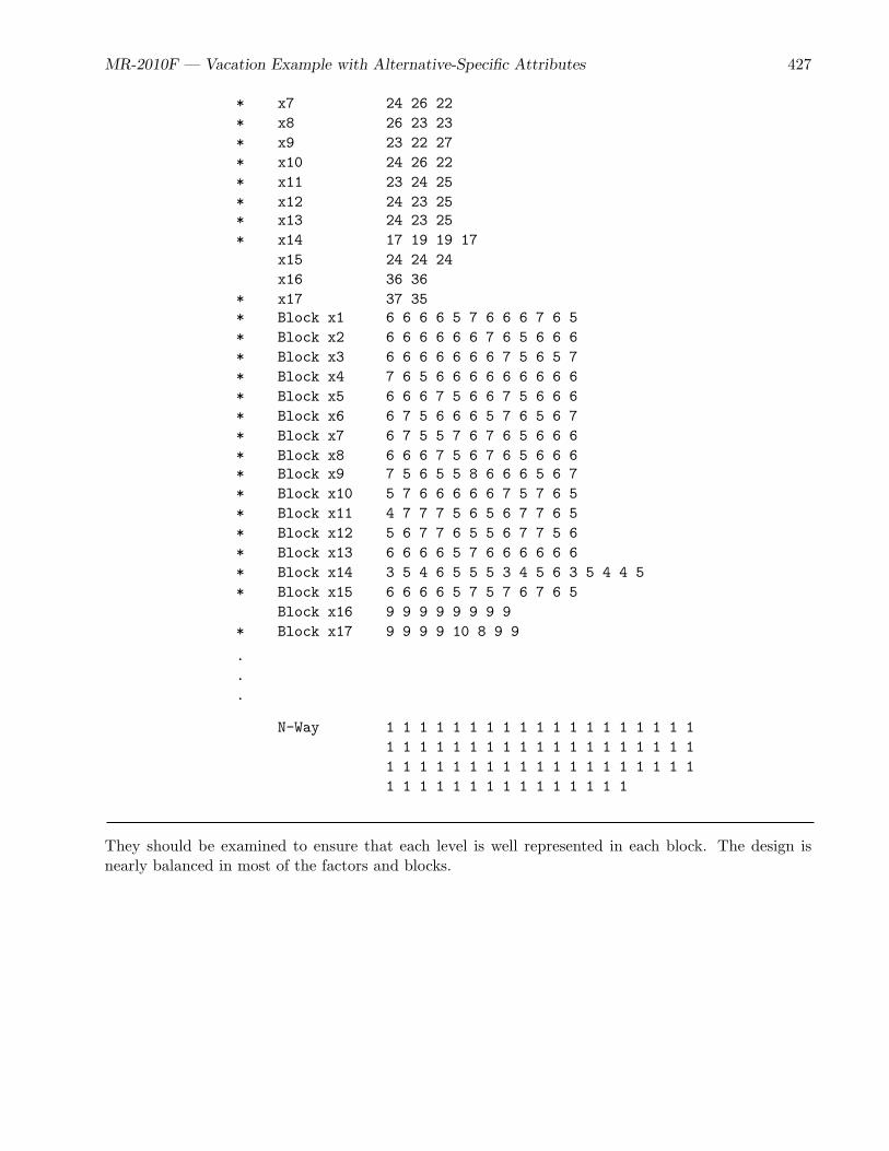
MR-2010F — Vacation Example with Alternative-Specific Attributes 427
* x7 24 26 22* x8 26 23 23* x9 23 22 27* x10 24 26 22* x11 23 24 25* x12 24 23 25* x13 24 23 25* x14 17 19 19 17
x15 24 24 24x16 36 36
* x17 37 35* Block x1 6 6 6 6 5 7 6 6 6 7 6 5* Block x2 6 6 6 6 6 6 7 6 5 6 6 6* Block x3 6 6 6 6 6 6 6 7 5 6 5 7* Block x4 7 6 5 6 6 6 6 6 6 6 6 6* Block x5 6 6 6 7 5 6 6 7 5 6 6 6* Block x6 6 7 5 6 6 6 5 7 6 5 6 7* Block x7 6 7 5 5 7 6 7 6 5 6 6 6* Block x8 6 6 6 7 5 6 7 6 5 6 6 6* Block x9 7 5 6 5 5 8 6 6 6 5 6 7* Block x10 5 7 6 6 6 6 6 7 5 7 6 5* Block x11 4 7 7 7 5 6 5 6 7 7 6 5* Block x12 5 6 7 7 6 5 5 6 7 7 5 6* Block x13 6 6 6 6 5 7 6 6 6 6 6 6* Block x14 3 5 4 6 5 5 5 3 4 5 6 3 5 4 4 5* Block x15 6 6 6 6 5 7 5 7 6 7 6 5
Block x16 9 9 9 9 9 9 9 9* Block x17 9 9 9 9 10 8 9 9
.
.
.
N-Way 1 1 1 1 1 1 1 1 1 1 1 1 1 1 1 1 1 1 11 1 1 1 1 1 1 1 1 1 1 1 1 1 1 1 1 1 11 1 1 1 1 1 1 1 1 1 1 1 1 1 1 1 1 1 11 1 1 1 1 1 1 1 1 1 1 1 1 1 1
They should be examined to ensure that each level is well represented in each block. The design isnearly balanced in most of the factors and blocks.

428 MR-2010F — Discrete Choice
Collecting data is time consuming and expensive. Before collecting data, it is a good practice to convertyour linear arrangement into a choice design and evaluate it in the context of a choice model. We startby creating some formats for the factor levels and the key to converting the linear arrangement into achoice design as follows:∗
proc format;value price 1 = ’ 999’ 2 = ’1249’ 3 = ’1499’ 4 = ’1749’ . = ’ ’;value scene 1 = ’Mountains’ 2 = ’Lake’ 3 = ’Beach’ . = ’ ’;value lodge 1 = ’Cabin’ 2 = ’Bed & Breakfast’ 3 = ’Hotel’ . = ’ ’;value side 1 = ’Side Trip’ 2 = ’No’ . = ’ ’;run;
data key;input Place $ 1-10 (Lodge Scene Price Side) ($);datalines;
Hawaii x1 x6 x11 x16Alaska x2 x7 x12 .Mexico x3 x8 x13 x17California x4 x9 x14 .Maine x5 x10 x15 .. . . . .;
For analysis, the design has five attributes. Place is the alternative name. Lodge, Scene, Price andSide are created from the design using the indicated factors. See page 356 for more information aboutcreating the design key. Notice that Side only applies to some of the alternatives and hence has missingvalues for the others. Processing the design and merging it with the data are similar to the exampleson pages 356 and 371. One difference is now there are asymmetries in Price. For Hawaii’s price, x11,we need to change 1, 2, and 3 to $1249, $1499, and $1749. For Alaska’s price, x12, we need to change1, 2, and 3 to $1249, $1499, and $1749. For Mexico’s price, x13, we need to change 1, 2, and 3 to $999,$1249, and $1499. For California’s price, x14, we need to change 1, 2, 3, and 4 to $999, $1249, $1499,and $1749. For Maine’s price, x11, we need to change 1, 2, and 3 to $999, $1249, and $1499. We cansimplify the problem by adding 1 to x11 and x12, which are the factors that start at $1249 insteadof $999. This lets us use a common format to set the price. See pages 499 and 884 for examples ofhandling more complicated asymmetries.
∗See page 67 for an explanation of the linear arrangement of a choice design versus the arrangement of a choice designthat is more suitable for analysis.

MR-2010F — Vacation Example with Alternative-Specific Attributes 429
The following steps process the design:
data temp;set sasuser.AsymVacLinDesBlckd(rename=(block=Form));x11 + 1;x12 + 1;run;
%mktroll(design=temp, key=key, alt=place, out=sasuser.AsymVacChDes,options=nowarn, keep=form)
data sasuser.AsymVacChDes;set sasuser.AsymVacChDes;format scene scene. lodge lodge. side side. price price.;run;
proc print data=sasuser.AsymVacChDes(obs=12);by form set; id form set;run;
The first two choice sets are as follows:
Vacation Example with Asymmetry
Form Set Place Lodge Scene Price Side
1 1 Hawaii Bed & Breakfast Lake 1499 NoAlaska Bed & Breakfast Mountains 1249Mexico Cabin Lake 999 NoCalifornia Cabin Lake 1249Maine Hotel Beach 1249
1 2 Hawaii Hotel Lake 1749 Side TripAlaska Hotel Lake 1499Mexico Hotel Beach 1249 NoCalifornia Cabin Beach 999Maine Cabin Lake 1249
Notice that each has six alternatives, one of which is displaying in this format as all blank.

430 MR-2010F — Discrete Choice
Testing the Design Before Data Collection
Collecting data is time consuming and expensive. It is always good practice to make sure that thedesign works with the most complicated model that we anticipate fitting. The following step evaluatesthe choice design:
title2 ’Evaluate the Choice Design’;
%choiceff(data=sasuser.AsymVacChDes,/* candidate set of choice sets */init=sasuser.AsymVacChDes(keep=set), /* select these sets */intiter=0, /* evaluate without internal iterations */
/* alternative-specific effects model *//* zero=none - no ref levels for place *//* order=data - do not sort levels */
model=class(place / zero=none order=data)/* zero=none - no ref levels any factor *//* order=formatted - sort levels *//* use blank sep to build interact terms*/
class(place * price place * scene place * lodge /zero=none order=formatted separators=’’ ’ ’)
/* no ref level for place *//* ref level for side is ’No’ *//* use blank sep to build interact terms*/
class(place * side / zero=’ ’ ’No’ separators=’’ ’ ’) /lprefix=0 /* lpr=0 labels created from just levels*/cprefix=0, /* cpr=0 names created from just levels */
nsets=72, /* number of choice sets */nalts=6, /* number of alternatives */beta=zero) /* assumed beta vector, Ho: b=0 */
We use the %ChoicEff macro to evaluate our choice design. You can both use this macro to search acandidate set for an efficient choice design, and you can use it to evaluate a design created by othermeans. The way you check a design like this is to first name it in the data= option. This is thecandidate set that contains all of the choice sets that we will consider. In addition, the same design isnamed in the init= option. The full specification is init=sasuser.AsymVacChDes(keep=set). Justthe variable Set is kept. It is used to bring in just the indicated choice sets from the data= design,which in this case is all of them. The option nsets=72 specifies the number of choice sets, and nalts=6specifies the number of alternatives. The option beta=zero specifies that we are assuming for designevaluation purpose that all of the betas or part-worth utilities are zero. You can evaluate the designfor other parameter vectors by specifying a list of numbers after beta=. This changes the variancesand standard errors. We also specify intiter=0 which specifies zero internal iterations. We use zerointernal iterations when we want to evaluate an initial design, but not attempt to improve it. The lastoption specifies the model.
The model specification contains everything that appears in the TRANSREG procedure’s model state-ment for coding the design. Many of these options should be familiar from previous examples. Thespecification class(place / zero=none order=data) names the place variable as a classificationvariable and asks for coded variables for every nonmissing level (zero=none). The order of the levelson output matches the order that the levels are first encountered in the input data set. This specificationcreates the alternative effects or alternative-specific intercepts.
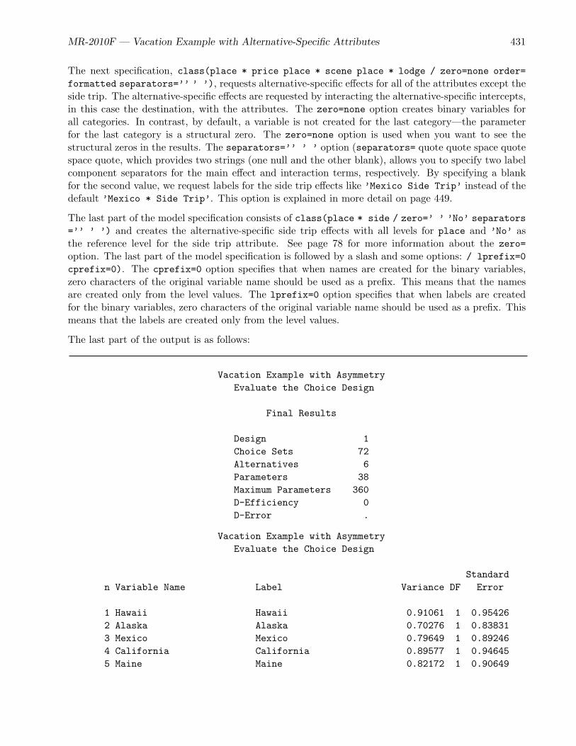
MR-2010F — Vacation Example with Alternative-Specific Attributes 431
The next specification, class(place * price place * scene place * lodge / zero=none order=formatted separators=’’ ’ ’), requests alternative-specific effects for all of the attributes except theside trip. The alternative-specific effects are requested by interacting the alternative-specific intercepts,in this case the destination, with the attributes. The zero=none option creates binary variables forall categories. In contrast, by default, a variable is not created for the last category—the parameterfor the last category is a structural zero. The zero=none option is used when you want to see thestructural zeros in the results. The separators=’’ ’ ’ option (separators= quote quote space quotespace quote, which provides two strings (one null and the other blank), allows you to specify two labelcomponent separators for the main effect and interaction terms, respectively. By specifying a blankfor the second value, we request labels for the side trip effects like ’Mexico Side Trip’ instead of thedefault ’Mexico * Side Trip’. This option is explained in more detail on page 449.
The last part of the model specification consists of class(place * side / zero=’ ’ ’No’ separators=’’ ’ ’) and creates the alternative-specific side trip effects with all levels for place and ’No’ asthe reference level for the side trip attribute. See page 78 for more information about the zero=option. The last part of the model specification is followed by a slash and some options: / lprefix=0cprefix=0). The cprefix=0 option specifies that when names are created for the binary variables,zero characters of the original variable name should be used as a prefix. This means that the namesare created only from the level values. The lprefix=0 option specifies that when labels are createdfor the binary variables, zero characters of the original variable name should be used as a prefix. Thismeans that the labels are created only from the level values.
The last part of the output is as follows:
Vacation Example with AsymmetryEvaluate the Choice Design
Final Results
Design 1Choice Sets 72Alternatives 6Parameters 38Maximum Parameters 360D-Efficiency 0D-Error .
Vacation Example with AsymmetryEvaluate the Choice Design
Standardn Variable Name Label Variance DF Error
1 Hawaii Hawaii 0.91061 1 0.954262 Alaska Alaska 0.70276 1 0.838313 Mexico Mexico 0.79649 1 0.892464 California California 0.89577 1 0.946455 Maine Maine 0.82172 1 0.90649

432 MR-2010F — Discrete Choice
6 Alaska_999 Alaska 999 . 0 .7 Alaska_1249 Alaska 1249 0.59635 1 0.772238 Alaska_1499 Alaska 1499 0.60551 1 0.778149 Alaska_1749 Alaska 1749 . 0 .10 California_999 California 999 0.85492 1 0.9246211 California_1249 California 1249 0.81130 1 0.9007212 California_1499 California 1499 0.82552 1 0.9085813 California_1749 California 1749 . 0 .14 Hawaii_999 Hawaii 999 . 0 .15 Hawaii_1249 Hawaii 1249 0.60792 1 0.7796916 Hawaii_1499 Hawaii 1499 0.59679 1 0.7725217 Hawaii_1749 Hawaii 1749 . 0 .18 Maine_999 Maine 999 0.60676 1 0.7789419 Maine_1249 Maine 1249 0.61109 1 0.7817220 Maine_1499 Maine 1499 . 0 .21 Maine_1749 Maine 1749 . 0 .22 Mexico_999 Mexico 999 0.59178 1 0.7692723 Mexico_1249 Mexico 1249 0.60604 1 0.7784924 Mexico_1499 Mexico 1499 . 0 .25 Mexico_1749 Mexico 1749 . 0 .26 AlaskaBeach Alaska Beach 0.63778 1 0.7986127 AlaskaLake Alaska Lake 0.58330 1 0.7637428 AlaskaMountains Alaska Mountains . 0 .29 CaliforniaBeach California Beach 0.59453 1 0.7710630 CaliforniaLake California Lake 0.67196 1 0.8197331 CaliforniaMountains California Mountains . 0 .32 HawaiiBeach Hawaii Beach 0.63923 1 0.7995233 HawaiiLake Hawaii Lake 0.61115 1 0.7817634 HawaiiMountains Hawaii Mountains . 0 .35 MaineBeach Maine Beach 0.63688 1 0.7980536 MaineLake Maine Lake 0.58479 1 0.7647137 MaineMountains Maine Mountains . 0 .38 MexicoBeach Mexico Beach 0.59462 1 0.7711139 MexicoLake Mexico Lake 0.59710 1 0.7727240 MexicoMountains Mexico Mountains . 0 .41 AlaskaBed___Breakfast Alaska Bed & Breakfast 0.62130 1 0.7882342 AlaskaCabin Alaska Cabin 0.61012 1 0.7811043 AlaskaHotel Alaska Hotel . 0 .44 CaliforniaBed___Breakfast California Bed & Breakfast 0.62122 1 0.7881745 CaliforniaCabin California Cabin 0.60866 1 0.7801646 CaliforniaHotel California Hotel . 0 .47 HawaiiBed___Breakfast Hawaii Bed & Breakfast 0.61876 1 0.7866148 HawaiiCabin Hawaii Cabin 0.59145 1 0.7690649 HawaiiHotel Hawaii Hotel . 0 .50 MaineBed___Breakfast Maine Bed & Breakfast 0.61592 1 0.7848051 MaineCabin Maine Cabin 0.60681 1 0.7789852 MaineHotel Maine Hotel . 0 .53 MexicoBed___Breakfast Mexico Bed & Breakfast 0.61050 1 0.7813454 MexicoCabin Mexico Cabin 0.61670 1 0.7853055 MexicoHotel Mexico Hotel . 0 .

MR-2010F — Vacation Example with Alternative-Specific Attributes 433
56 AlaskaSide_Trip Alaska Side Trip . 0 .57 CaliforniaSide_Trip California Side Trip . 0 .58 HawaiiSide_Trip Hawaii Side Trip 0.40413 1 0.6357259 MaineSide_Trip Maine Side Trip . 0 .60 MexicoSide_Trip Mexico Side Trip 0.40622 1 0.63735
==38
It consists of a table with the name and label for each parameter along with its variance, df, andstandard error. It needs to be carefully evaluated to see if the zeros and nonzeros are in all of theright places. We see one parameter for five of the six destinations, with the constant stay-at-homealternative in all cases excluded from the table. This is followed by four terms for the Alaska priceeffect. The Alaska at $999 parameter is zero since $999 does not apply to Alaska. The Alaska at $1749parameter is the reference level and hence is zero. The other two Alaska price parameters are nonzero.Similarly, each of the alternative-specific price effects have two or three parameters (the number ofapplicable prices minus one). For the scenery and accommodations attributes, each alternative has twononzero parameters and a reference level. There are two nonzero parameters for the side trips for thetwo applicable destinations. The pattern of zeros and nonzeros looks perfect. There are 38 parametersin the alternative-specific model.
You should also note that the variances and standard errors. They are all approximately the sameorder of magnitude. Sometimes you might see wildly varying parameters. This is usually a sign of aproblematic design, perhaps one with too few choice sets for the number of parameters. This designlooks good. The number of parameters in our model is 38 and the maximum number we could estimatewith this design is 360, so too few choice sets should not be a problem. Note one difference betweenthese results and the results that we see in the previous example on page 361. Here, our standarderrors are not constant within an attribute, although they are similar. This is because none of ourfactors are orthogonal, although they are close.
Generating the Questionnaire
The following step produces the questionnaire:
%let m = 6; /* m alts including constant */%let mm1 = %eval(&m - 1); /* m - 1 */%let n = 18; /* number of choice sets */%let blocks = 4; /* number of blocks */
title;options ls=80 ps=60 nonumber nodate;
data _null_;array dests[&mm1] $ 10 _temporary_ (’Hawaii’ ’Alaska’ ’Mexico’
’California’ ’Maine’);array scenes[3] $ 13 _temporary_
(’the Mountains’ ’a Lake’ ’the Beach’);

434 MR-2010F — Discrete Choice
array lodging[3] $ 15 _temporary_(’Cabin’ ’Bed & Breakfast’ ’Hotel’);
array x[15];
array p[&mm1];length price $ 6;file print linesleft=ll;
set sasuser.AsymVacLinDesBlckd;by block;
p1 = 1499 + (x[11] - 2) * 250;p2 = 1499 + (x[12] - 2) * 250;p3 = 1249 + (x[13] - 2) * 250;p4 = 1374 + (x[14] - 2.5) * 250;p5 = 1249 + (x[15] - 2) * 250;
if first.block then do;choice = 0;put _page_;put @50 ’Form: ’ block ’ Subject: ________’ //;end;
choice + 1;
if ll < (19 + (x16 = 1) + (x17 = 1)) then put _page_;put choice 2. ’) Circle your choice of ’
’vacation destinations:’ /;
do dest = 1 to &mm1;price = left(put(p[dest], dollar6.));put ’ ’ dest 1. ’) ’ dests[dest]
+(-1) ’, staying in a ’ lodging[x[dest]]’near ’ scenes[x[&mm1 + dest]] +(-1) ’,’ /+7 ’with a package cost of ’ price +(-1) @@;
if dest = 3 and x16 = 1 thenput ’, and an optional visit’ / +7
’to archaeological sites for an additional $100’ @@;else if dest = 1 and x17 = 1 then
put ’, and an optional helicopter’ / +7’flight to an active volcano for an additional $200’ @@;
put ’.’ /;end;
put " &m) Stay at home this year." /;run;

MR-2010F — Vacation Example with Alternative-Specific Attributes 435
The first two choice sets for the first subject are as follows:
Form: 1 Subject: ________
1) Circle your choice of vacation destinations:
1) Hawaii, staying in a Bed & Breakfast near a Lake,with a package cost of $1,499.
2) Alaska, staying in a Bed & Breakfast near the Mountains,with a package cost of $1,249.
3) Mexico, staying in a Cabin near a Lake,with a package cost of $999.
4) California, staying in a Cabin near a Lake,with a package cost of $1,249.
5) Maine, staying in a Hotel near the Beach,with a package cost of $1,249.
6) Stay at home this year.
2) Circle your choice of vacation destinations:
1) Hawaii, staying in a Hotel near a Lake,with a package cost of $1,749.
2) Alaska, staying in a Hotel near a Lake,with a package cost of $1,499.
3) Mexico, staying in a Hotel near the Beach,with a package cost of $1,249, and an optional visitto archaeological sites for an additional $100.
4) California, staying in a Cabin near the Beach,with a package cost of $999.
5) Maine, staying in a Cabin near a Lake,with a package cost of $1,249.
6) Stay at home this year.

436 MR-2010F — Discrete Choice
In practice, data collection is typically be much more elaborate than this. It might involve art work orphotographs, and the choice sets might be presented and the data might be collected through personalinterview or over the Web. However the choice sets are presented and the data are collected, theessential elements remain the same. Subjects are shown a set of alternatives and are asked to make achoice, then they go on to the next set.
Generating Artificial Data
This section shows in a cursory way how to generate artificial data. Some researchers wisely like touse artificial data to test a design before spending lots of money on collecting data. See the sectionbeginning on page 393 for a detailed discussion of generating artificial data.
The following step generates an artificial set of data:
data _null_;array dests[&mm1] _temporary_ (5 -1 4 3 2);array scenes[3] _temporary_ (-1 0 1);array lodging[3] _temporary_ (0 3 2);array u[&m];array x[15];
do rep = 1 to 100;n = 0;do i = 1 to &blocks;
k + 1;if mod(k,3) = 1 then put;put k 3. +1 i 1. +2 @@;
do j = 1 to &n; n + 1;set sasuser.AsymVacLinDesBlckd point=n;do dest = 1 to &mm1;
u[dest] = dests[dest] + lodging[x[dest]] +scenes[x[&mm1 + dest]] -x[2 * &mm1 + dest] +2 * normal(17);
end;
u[1] = u[1] + (x16 = 1);u[3] = u[3] + (x17 = 1);u&m = -3 + 3 * normal(17);m = max(of u1-u&m);if abs(u1 - m) < 1e-4 then c = 1;else if abs(u2 - m) < 1e-4 then c = 2;else if abs(u3 - m) < 1e-4 then c = 3;else if abs(u4 - m) < 1e-4 then c = 4;else if abs(u5 - m) < 1e-4 then c = 5;else c = 6;put +(-1) c @@;end;
end;end;
stop;run;

MR-2010F — Vacation Example with Alternative-Specific Attributes 437
Collecting data is time consuming and expensive. Generating some artificial data before the data arecollected to test your code and make sure the analysis will run is a good idea. It helps avoid the “Howam I going to analyze this?” question from occurring after the data have already been collected. Thisstep generates data for 400 subjects, 100 per block.
The dests, scenes, and lodging arrays are initialized with part-worth utilities for each level. Theutilities for each of the destinations are computed and stored in the array u in the statement u[dest]= ..., which includes an error term 2 * normal(17). The utilities for the side trips are added in sep-arately with u[1] = u[1] + (x16 = 1) and u[3] = u[3] + (x17 = 1). The utility for the stay-at-home alternative is -3 + 3 * normal(17). The maximum utility is computed, m = max(of u1-u&m)and the alternative with the maximum utility is chosen. The put statement writes out the results tothe log.
Reading, Processing, and Analyzing the Data
The results from the previous step are pasted into a DATA step and run to mimic reading real inputdata as follows:
title ’Vacation Example with Asymmetry’;
data results;input Subj Form (choose1-choose&n) (1.) @@;datalines;
1 1 413414111315351335 2 2 115311141441134121 3 3 3314513444335133414 4 113111143133311314 5 1 113413531545431313 6 2 1451311114143315117 3 313413113111313331 8 4 415143311133541321 9 1 133314111133431113...
;
The analysis proceeds in a fashion similar to the simpler vacation example on page 371. The followingsteps merge the data and display a subset of the results:
%mktmerge(design=sasuser.AsymVacChDes, data=results, out=res2, blocks=form,nsets=&n, nalts=&m, setvars=choose1-choose&n,stmts=%str(price = input(put(price, price.), 5.);
format scene scene. lodge lodge. side side.;))
proc print data=res2(obs=18);id form subj set; by form subj set;run;
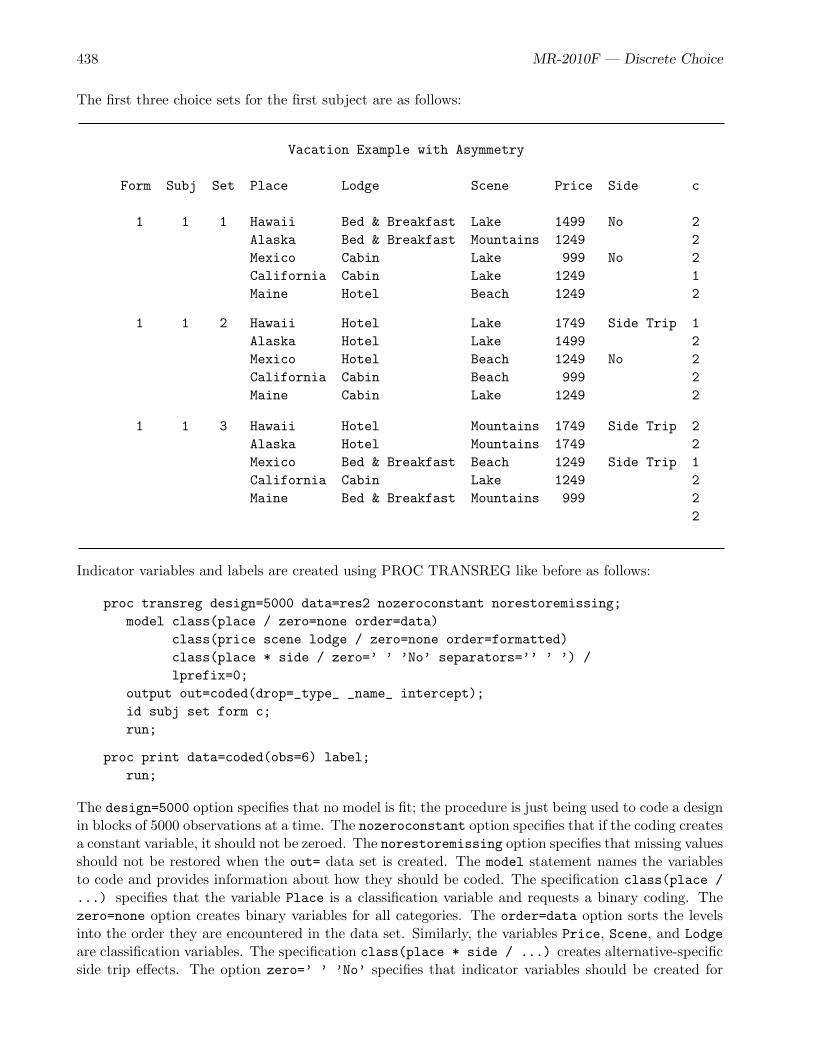
438 MR-2010F — Discrete Choice
The first three choice sets for the first subject are as follows:
Vacation Example with Asymmetry
Form Subj Set Place Lodge Scene Price Side c
1 1 1 Hawaii Bed & Breakfast Lake 1499 No 2Alaska Bed & Breakfast Mountains 1249 2Mexico Cabin Lake 999 No 2California Cabin Lake 1249 1Maine Hotel Beach 1249 2
1 1 2 Hawaii Hotel Lake 1749 Side Trip 1Alaska Hotel Lake 1499 2Mexico Hotel Beach 1249 No 2California Cabin Beach 999 2Maine Cabin Lake 1249 2
1 1 3 Hawaii Hotel Mountains 1749 Side Trip 2Alaska Hotel Mountains 1749 2Mexico Bed & Breakfast Beach 1249 Side Trip 1California Cabin Lake 1249 2Maine Bed & Breakfast Mountains 999 2
2
Indicator variables and labels are created using PROC TRANSREG like before as follows:
proc transreg design=5000 data=res2 nozeroconstant norestoremissing;model class(place / zero=none order=data)
class(price scene lodge / zero=none order=formatted)class(place * side / zero=’ ’ ’No’ separators=’’ ’ ’) /lprefix=0;
output out=coded(drop=_type_ _name_ intercept);id subj set form c;run;
proc print data=coded(obs=6) label;run;
The design=5000 option specifies that no model is fit; the procedure is just being used to code a designin blocks of 5000 observations at a time. The nozeroconstant option specifies that if the coding createsa constant variable, it should not be zeroed. The norestoremissing option specifies that missing valuesshould not be restored when the out= data set is created. The model statement names the variablesto code and provides information about how they should be coded. The specification class(place /...) specifies that the variable Place is a classification variable and requests a binary coding. Thezero=none option creates binary variables for all categories. The order=data option sorts the levelsinto the order they are encountered in the data set. Similarly, the variables Price, Scene, and Lodgeare classification variables. The specification class(place * side / ...) creates alternative-specificside trip effects. The option zero=’ ’ ’No’ specifies that indicator variables should be created for

MR-2010F — Vacation Example with Alternative-Specific Attributes 439
all levels of Place except blank, and all levels of Side except ’No’. The specification zero=’ ’ isalmost the same as zero=none. The zero=’ ’ specification names a missing level as the reference levelcreating indicator variables for all nonmissing levels of the class variables, just like zero=none. Thedifference is zero=none applies to all of the variables named in the class specification. When youwant zero=none to apply to only some variables, then you must use zero=’ ’, as in zero=’ ’ ’No’instead. In this case, zero=none applies to the first variable and zero=’No’ applies to the second.With zero=’ ’, PROC TRANSREG displays the following warning, which can be safely ignored:
WARNING: Reference level ZERO=’’ was not found for variable Place.
See page 78 for more information about the zero= option.
The separators=’’ ’ ’ option (separators= quote quote space quote space quote) allows you tospecify two label component separators for the main effect and interaction terms, respectively. Byspecifying a blank for the second value, we request labels for the side trip effects like ’Mexico SideTrip’ instead of the default ’Mexico * Side Trip’. This option is explained in more detail on page449.
The lprefix=0 option specifies that when labels are created for the binary variables, zero charactersof the original variable name should be used as a prefix. This means that the labels are created onlyfrom the level values. An output statement names the output data set and drops variables that arenot needed. Finally, the id statement names the additional variables that we want copied from theinput to the output data set. The results are as follows:
Vacation Example with Asymmetry
Obs Hawaii Alaska Mexico California Maine 999 1249 1499 1749 Beach Lake
1 1 0 0 0 0 0 0 1 0 0 12 0 1 0 0 0 0 1 0 0 0 03 0 0 1 0 0 1 0 0 0 0 14 0 0 0 1 0 0 1 0 0 0 15 0 0 0 0 1 0 1 0 0 1 06 0 0 0 0 0 0 0 0 0 0 0
Alaska Hawaii Maine MexicoBed & Side California Side Side Side
Obs Mountains Breakfast Cabin Hotel Trip Side Trip Trip Trip Trip
1 0 1 0 0 0 0 0 0 02 1 1 0 0 0 0 0 0 03 0 0 1 0 0 0 0 0 04 0 0 1 0 0 0 0 0 05 0 0 0 1 0 0 0 0 06 0 0 0 0 0 0 0 0 0

440 MR-2010F — Discrete Choice
Obs Place Price Scene Lodge Side Subj Set Form c
1 Hawaii 1499 Lake Bed & Breakfast No 1 1 1 22 Alaska 1249 Mountains Bed & Breakfast 1 1 1 23 Mexico 999 Lake Cabin No 1 1 1 24 California 1249 Lake Cabin 1 1 1 15 Maine 1249 Beach Hotel 1 1 1 26 1 1 1 2
The PROC PHREG specification is the same as we have used before. Recall that we used %phchoice(on)on page 287 to customize the output from PROC PHREG.) The following step analyzes the data:
proc phreg data=coded brief;model c*c(2) = &_trgind / ties=breslow;strata subj set;run;
The results are as follows:
Vacation Example with Asymmetry
The PHREG Procedure
Model Information
Data Set WORK.CODEDDependent Variable cCensoring Variable cCensoring Value(s) 2Ties Handling BRESLOW
Number of Observations Read 43200Number of Observations Used 43200
Summary of Subjects, Sets, and Chosen and Unchosen Alternatives
Number of Number of Chosen NotPattern Choices Alternatives Alternatives Chosen
1 7200 6 1 5
Convergence Status
Convergence criterion (GCONV=1E-8) satisfied.

MR-2010F — Vacation Example with Alternative-Specific Attributes 441
Model Fit Statistics
Without WithCriterion Covariates Covariates
-2 LOG L 25801.336 12603.247AIC 25801.336 12631.247SBC 25801.336 12727.593
Testing Global Null Hypothesis: BETA=0
Test Chi-Square DF Pr > ChiSq
Likelihood Ratio 13198.0891 14 <.0001Score 12223.0125 14 <.0001Wald 5081.3295 14 <.0001
Multinomial Logit Parameter Estimates
Parameter StandardDF Estimate Error Chi-Square Pr > ChiSq
Hawaii 1 3.61141 0.22224 264.0701 <.0001Alaska 1 -0.94997 0.26364 12.9836 0.0003Mexico 1 2.26877 0.22776 99.2247 <.0001California 1 1.54548 0.22760 46.1102 <.0001Maine 1 0.74153 0.23210 10.2074 0.0014999 1 2.10214 0.07298 829.7619 <.0001
1249 1 1.44298 0.06078 563.6949 <.00011499 1 0.72311 0.05936 148.4188 <.00011749 0 0 . . .Beach 1 1.42021 0.04635 938.8384 <.0001Lake 1 0.72019 0.04472 259.3676 <.0001Mountains 0 0 . . .Bed & Breakfast 1 0.65045 0.04079 254.3369 <.0001Cabin 1 -1.42317 0.04809 875.8795 <.0001Hotel 0 0 . . .Alaska Side Trip 0 0 . . .California Side Trip 0 0 . . .Hawaii Side Trip 1 0.71850 0.05753 155.9801 <.0001Maine Side Trip 0 0 . . .Mexico Side Trip 1 0.65550 0.06293 108.4863 <.0001
You would not expect the part-worth utilities to match those that are used to generate the data, butyou would expect a similar ordering within each attribute, and in fact that does occur. These datacan also be analyzed with quantitative price effects and destination by attribute interactions, as in theprevious vacation example.

442 MR-2010F — Discrete Choice
Aggregating the Data
This data set is rather large with 43,200 observations. You can make the analysis run faster and withless memory by aggregating. Instead of stratifying on each choice set and subject combination, youcan stratify just on choice set and specify the number of times each alternative is chosen and thenumber of times it is not chosen. First, use PROC SUMMARY to count the number of times eachobservation occurs. Specify all the analysis variables, and in this example, also specify Form. Thevariable Form is added to the list because Set designates choice set within form. It is the Form andSet combinations that identify the choice sets. (In the previous PROC PHREG step, since the Subj* Set combinations uniquely identified each stratum, Form is not needed.) PROC SUMMARY storesthe number of times each unique observation appears in the variable freq . PROC PHREG is thenrun with a freq statement. Now, instead of analyzing a data set with 43,200 observations and 7200strata, we analyze a data set with at most 2× 6× 72 = 864 observations and 72 strata. For each of the6 alternatives and 72 choice sets, there are typically 2 observations in the aggregate data set: one thatcontains the number of times it is chosen and one that contains the number of times it is not chosen.When one of those counts is zero, there is one observation. In this case, the aggregate data set has 724observations. The following steps aggregate and perform the analysis:
proc summary data=coded nway;class form set c &_trgind;output out=agg(drop=_type_);run;
proc phreg data=agg;model c*c(2) = &_trgind / ties=breslow;freq _freq_;strata form set;run;
PROC SUMMARY ran in three seconds, and PROC PHREG ran in less than one second. The resultsare as follows:
Vacation Example with Asymmetry
The PHREG Procedure
Model Information
Data Set WORK.AGGDependent Variable cCensoring Variable cCensoring Value(s) 2Frequency Variable _FREQ_Ties Handling BRESLOW
Number of Observations Read 724Number of Observations Used 724Sum of Frequencies Read 43200Sum of Frequencies Used 43200

MR-2010F — Vacation Example with Alternative-Specific Attributes 443
Summary of Subjects, Sets, and Chosen and Unchosen Alternatives
Number of Chosen NotStratum Form Set Alternatives Alternatives Chosen
1 1 1 600 100 5002 1 2 600 100 5003 1 3 600 100 5004 1 4 600 100 500...71 4 71 600 100 50072 4 72 600 100 500
---------------------------------------------------------------------------Total 43200 7200 36000
The parameter estimates and Chi-Square statistics (not shown) are the same as before. The summarytable shows the results of the aggregation, 100 out of 600 alternatives are chosen in each stratum. Thelog likelihood statistics are different, but that does not matter since the Chi-Square statistics are thesame. Page 466 provides more information about this.

444 MR-2010F — Discrete Choice
Brand Choice Example with Aggregate Data
In this next example, subjects are presented with brands of a product at different prices. There arefour brands and a constant alternative, eight choice sets, and 100 subjects. This example shows how tohandle data that come to you already aggregated. It also illustrates comparing the fits of two competingmodels, the mother logit model, cross-effects, IIA, and techniques for handling large data sets. Thechoice sets, with the price of each alternative and the number of times it is chosen, are shown next.
Set Brand 1 Brand 2 Brand 3 Brand 4 Other1 $3.99 4 $5.99 29 $3.99 16 $5.99 42 $4.99 92 $5.99 12 $5.99 19 $5.99 22 $5.99 33 $4.99 143 $5.99 34 $5.99 26 $3.99 8 $3.99 27 $4.99 54 $5.99 13 $3.99 37 $5.99 15 $3.99 27 $4.99 85 $5.99 49 $3.99 1 $3.99 9 $5.99 37 $4.99 46 $3.99 31 $5.99 12 $5.99 6 $3.99 18 $4.99 337 $3.99 37 $3.99 10 $5.99 5 $5.99 35 $4.99 138 $3.99 16 $3.99 14 $3.99 5 $3.99 51 $4.99 14
The first choice set consists of Brand 1 at $3.99, Brand 2 at $5.99, Brand 3 at $3.99, Brand 4 at $5.99,and Other at $4.99. From this choice set, Brand 1 is chosen 4 times, Brand 2 is chosen 29 times, Brand3 is chosen 16 times, Brand 4 is chosen 42 times, and Other is chosen 9 times.
Processing the Data
As in the previous examples, we process the data to create a data set with one stratum for eachchoice set within each subject and m alternatives per stratum. This example has 100 people times 5alternatives times 8 choice sets equals 4000 observations. The first five observations are for the firstsubject and the first choice set, the next five observations are for the second subject and the first choiceset, ..., the next five observations are for the one-hundredth subject and the first choice set, the nextfive observations are for the first subject and the second choice set, and so on. Subject 1 in the firstchoice set is almost certainly not the same as subject 1 in subsequent choice sets since we are givenaggregate data. However, that is not important. What is important is that we have a subject andchoice set variable whose unique combinations identify each choice set within each subject. In previousexamples, we specified strata Subj Set with PROC PHREG, and our data are sorted by choice setwithin subject. We can still use the same specification even though our data are now sorted by subjectwithin choice set. The following step reads and prepares the data:
%let m = 5; /* Number of Brands in Each Choice Set *//* (including Other) */
title ’Brand Choice Example, Multinomial Logit Model’;
proc format;value brand 1 = ’Brand 1’ 2 = ’Brand 2’ 3 = ’Brand 3’
4 = ’Brand 4’ 5 = ’Other’;run;
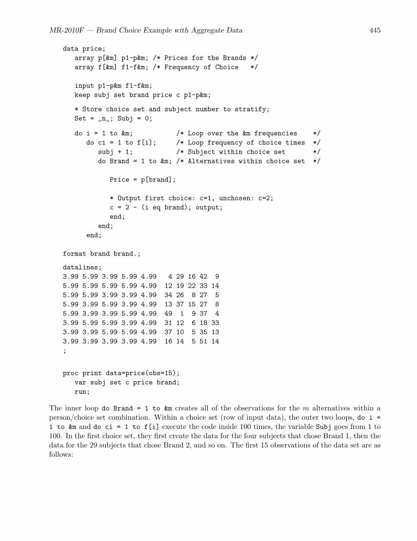
MR-2010F — Brand Choice Example with Aggregate Data 445
data price;array p[&m] p1-p&m; /* Prices for the Brands */array f[&m] f1-f&m; /* Frequency of Choice */
input p1-p&m f1-f&m;keep subj set brand price c p1-p&m;
* Store choice set and subject number to stratify;Set = _n_; Subj = 0;
do i = 1 to &m; /* Loop over the &m frequencies */do ci = 1 to f[i]; /* Loop frequency of choice times */
subj + 1; /* Subject within choice set */do Brand = 1 to &m; /* Alternatives within choice set */
Price = p[brand];
* Output first choice: c=1, unchosen: c=2;c = 2 - (i eq brand); output;end;
end;end;
format brand brand.;
datalines;3.99 5.99 3.99 5.99 4.99 4 29 16 42 95.99 5.99 5.99 5.99 4.99 12 19 22 33 145.99 5.99 3.99 3.99 4.99 34 26 8 27 55.99 3.99 5.99 3.99 4.99 13 37 15 27 85.99 3.99 3.99 5.99 4.99 49 1 9 37 43.99 5.99 5.99 3.99 4.99 31 12 6 18 333.99 3.99 5.99 5.99 4.99 37 10 5 35 133.99 3.99 3.99 3.99 4.99 16 14 5 51 14;
proc print data=price(obs=15);var subj set c price brand;run;
The inner loop do Brand = 1 to &m creates all of the observations for the m alternatives within aperson/choice set combination. Within a choice set (row of input data), the outer two loops, do i =1 to &m and do ci = 1 to f[i] execute the code inside 100 times, the variable Subj goes from 1 to100. In the first choice set, they first create the data for the four subjects that chose Brand 1, then thedata for the 29 subjects that chose Brand 2, and so on. The first 15 observations of the data set are asfollows:

446 MR-2010F — Discrete Choice
Brand Choice Example, Multinomial Logit Model
Obs Subj Set c Price Brand
1 1 1 1 3.99 Brand 12 1 1 2 5.99 Brand 23 1 1 2 3.99 Brand 34 1 1 2 5.99 Brand 45 1 1 2 4.99 Other6 2 1 1 3.99 Brand 17 2 1 2 5.99 Brand 28 2 1 2 3.99 Brand 39 2 1 2 5.99 Brand 410 2 1 2 4.99 Other11 3 1 1 3.99 Brand 112 3 1 2 5.99 Brand 213 3 1 2 3.99 Brand 314 3 1 2 5.99 Brand 415 3 1 2 4.99 Other
Note that the data set also contains the variables p1-p5 which contain the prices of each of thealternatives. These variables, which are used in constructing the cross-effects, are discussed in moredetail on page 452. The following step displays the first five rows:
proc print data=price(obs=5); run;
The results are as follows:
Brand Choice Example, Multinomial Logit Model
Obs p1 p2 p3 p4 p5 Set Subj Brand Price c
1 3.99 5.99 3.99 5.99 4.99 1 1 Brand 1 3.99 12 3.99 5.99 3.99 5.99 4.99 1 1 Brand 2 5.99 23 3.99 5.99 3.99 5.99 4.99 1 1 Brand 3 3.99 24 3.99 5.99 3.99 5.99 4.99 1 1 Brand 4 5.99 25 3.99 5.99 3.99 5.99 4.99 1 1 Other 4.99 2

MR-2010F — Brand Choice Example with Aggregate Data 447
Simple Price Effects
The data are coded using PROC TRANSREG as follows:
proc transreg design data=price nozeroconstant norestoremissing;model class(brand / zero=none) identity(price) / lprefix=0;output out=coded(drop=_type_ _name_ intercept);label price = ’Price’;id subj set c;run;
The design option specifies that no model is fit; the procedure is just being used to code a design. Thenozeroconstant option specifies that if the coding creates a constant variable, it should not be zeroed.The norestoremissing option specifies that missing values should not be restored when the out= dataset is created. The model statement names the variables to code and provides information about howthey should be coded. The specification class(brand / zero=none) specifies that the variable Brandis a classification variable and requests a binary coding. The zero=none option creates binary variablesfor all categories. The specification identity(price) specifies that the variable Price is quantitativeand hence should directly enter the model without coding. The lprefix=0 option specifies that whenlabels are created for the binary variables, zero characters of the original variable name should be usedas a prefix. This means that the labels are created only from the level values. An output statementnames the output data set and drops variables that are not needed. Finally, the id statement namesthe additional variables that we want copied from the input to the output data set. The following stepperforms the analysis:
proc phreg data=coded brief;title2 ’Discrete Choice with Common Price Effect’;model c*c(2) = &_trgind / ties=breslow;strata subj set;run;
Recall that we used %phchoice(on) on page 287 to customize the output from PROC PHREG. Theresults are as follows:
Brand Choice Example, Multinomial Logit ModelDiscrete Choice with Common Price Effect
The PHREG Procedure
Model Information
Data Set WORK.CODEDDependent Variable cCensoring Variable cCensoring Value(s) 2Ties Handling BRESLOW
Number of Observations Read 4000Number of Observations Used 4000
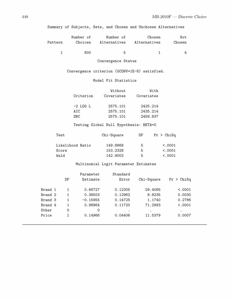
448 MR-2010F — Discrete Choice
Summary of Subjects, Sets, and Chosen and Unchosen Alternatives
Number of Number of Chosen NotPattern Choices Alternatives Alternatives Chosen
1 800 5 1 4
Convergence Status
Convergence criterion (GCONV=1E-8) satisfied.
Model Fit Statistics
Without WithCriterion Covariates Covariates
-2 LOG L 2575.101 2425.214AIC 2575.101 2435.214SBC 2575.101 2458.637
Testing Global Null Hypothesis: BETA=0
Test Chi-Square DF Pr > ChiSq
Likelihood Ratio 149.8868 5 <.0001Score 153.2328 5 <.0001Wald 142.9002 5 <.0001
Multinomial Logit Parameter Estimates
Parameter StandardDF Estimate Error Chi-Square Pr > ChiSq
Brand 1 1 0.66727 0.12305 29.4065 <.0001Brand 2 1 0.38503 0.12962 8.8235 0.0030Brand 3 1 -0.15955 0.14725 1.1740 0.2786Brand 4 1 0.98964 0.11720 71.2993 <.0001Other 0 0 . . .Price 1 0.14966 0.04406 11.5379 0.0007

MR-2010F — Brand Choice Example with Aggregate Data 449
Alternative-Specific Price Effects
In the following step, the data are coded for fitting a multinomial logit model with brand by priceeffects:
proc transreg design data=price nozeroconstant norestoremissing;model class(brand / zero=none separators=’’ ’ ’) |
identity(price) / lprefix=0;output out=coded(drop=_type_ _name_ intercept);label price = ’Price’;id subj set c;run;
The PROC TRANSREG model statement has a vertical bar, “|”, between the class specification andthe identity specification. Since the zero=none option is specified with class, the vertical bar createstwo sets of variables: five indicator variables for the brand effects and five more variables for the brandby price interactions. The separators= option allows you to specify two label component separatorsas quoted strings. The specification separators=’’ ’ ’ (separators= quote quote space quote spacequote) specifies a null string (quote quote) and a blank (quote space quote). The separators=’’ ’ ’option in the class specification specifies the separators that are used to construct the labels for themain effect and interaction terms, respectively. By default, the alternative-specific price effects—thebrand by price interactions—have labels like ’Brand 1 * Price’ since the default second value forseparators= is ’ * ’ (a quoted space asterisk space). Specifying ’ ’ (a quoted space) as the secondvalue creates labels of the form ’Brand 1 Price’. Since lprefix=0, the main-effects separator, whichis the first separators= value, ’’ (quote quote), is ignored. Zero name or input variable label charactersare used to construct the label. The label is simply the formatted value of the class variable. Thefollowing steps display the first two coded choice sets and perform the analysis:
proc print data=coded(obs=10) label;title2 ’Discrete Choice with Brand by Price Effects’;var subj set c brand price &_trgind;run;
proc phreg data=coded brief;model c*c(2) = &_trgind / ties=breslow;strata subj set;run;
title2;
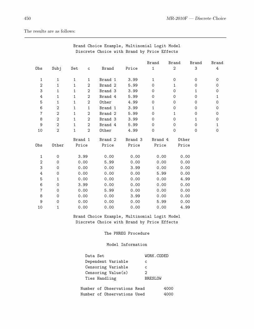
450 MR-2010F — Discrete Choice
The results are as follows:
Brand Choice Example, Multinomial Logit ModelDiscrete Choice with Brand by Price Effects
Brand Brand Brand BrandObs Subj Set c Brand Price 1 2 3 4
1 1 1 1 Brand 1 3.99 1 0 0 02 1 1 2 Brand 2 5.99 0 1 0 03 1 1 2 Brand 3 3.99 0 0 1 04 1 1 2 Brand 4 5.99 0 0 0 15 1 1 2 Other 4.99 0 0 0 06 2 1 1 Brand 1 3.99 1 0 0 07 2 1 2 Brand 2 5.99 0 1 0 08 2 1 2 Brand 3 3.99 0 0 1 09 2 1 2 Brand 4 5.99 0 0 0 110 2 1 2 Other 4.99 0 0 0 0
Brand 1 Brand 2 Brand 3 Brand 4 OtherObs Other Price Price Price Price Price
1 0 3.99 0.00 0.00 0.00 0.002 0 0.00 5.99 0.00 0.00 0.003 0 0.00 0.00 3.99 0.00 0.004 0 0.00 0.00 0.00 5.99 0.005 1 0.00 0.00 0.00 0.00 4.996 0 3.99 0.00 0.00 0.00 0.007 0 0.00 5.99 0.00 0.00 0.008 0 0.00 0.00 3.99 0.00 0.009 0 0.00 0.00 0.00 5.99 0.0010 1 0.00 0.00 0.00 0.00 4.99
Brand Choice Example, Multinomial Logit ModelDiscrete Choice with Brand by Price Effects
The PHREG Procedure
Model Information
Data Set WORK.CODEDDependent Variable cCensoring Variable cCensoring Value(s) 2Ties Handling BRESLOW
Number of Observations Read 4000Number of Observations Used 4000

MR-2010F — Brand Choice Example with Aggregate Data 451
Summary of Subjects, Sets, and Chosen and Unchosen Alternatives
Number of Number of Chosen NotPattern Choices Alternatives Alternatives Chosen
1 800 5 1 4
Convergence Status
Convergence criterion (GCONV=1E-8) satisfied.
Model Fit Statistics
Without WithCriterion Covariates Covariates
-2 LOG L 2575.101 2424.812AIC 2575.101 2440.812SBC 2575.101 2478.288
Testing Global Null Hypothesis: BETA=0
Test Chi-Square DF Pr > ChiSq
Likelihood Ratio 150.2891 8 <.0001Score 154.2563 8 <.0001Wald 143.1425 8 <.0001
Multinomial Logit Parameter Estimates
Parameter StandardDF Estimate Error Chi-Square Pr > ChiSq
Brand 1 1 -0.00972 0.43555 0.0005 0.9822Brand 2 1 -0.62230 0.48866 1.6217 0.2028Brand 3 1 -0.81250 0.60318 1.8145 0.1780Brand 4 1 0.31778 0.39549 0.6456 0.4217Other 0 0 . . .Brand 1 Price 1 0.13587 0.08259 2.7063 0.1000Brand 2 Price 1 0.20074 0.09210 4.7512 0.0293Brand 3 Price 1 0.13126 0.11487 1.3057 0.2532Brand 4 Price 1 0.13478 0.07504 3.2255 0.0725Other Price 0 0 . . .

452 MR-2010F — Discrete Choice
The likelihood for this model is essentially the same as for the simpler, common-price-slope model fitpreviously, −2 log(LC) = 2425.214 compared to 2424.812. You can test the null hypothesis that thetwo models are not significantly different by comparing their likelihoods. The difference between two−2 log(LC)’s (the number reported under ’With Covariates’ in the output) has a chi-square distribution.We can get the df for the test by subtracting the two df for the two likelihoods. The difference2425.214− 2424.812 = 0.402 is distributed χ2 with 8− 5 = 3 df and is not statistically significant.
Mother Logit Model
This next step fits the so-called “mother logit” model. This step creates the full design matrix, includingthe brand, price, and cross-effects. A cross-effect represents the effect of one alternative on the utilityof another alternative. First, the input data set for the first choice set is displayed by the followingstep:
proc print data=price(obs=5) label;run;
The results are as follows:
Brand Choice Example, Multinomial Logit Model
Obs p1 p2 p3 p4 p5 Set Subj Brand Price c
1 3.99 5.99 3.99 5.99 4.99 1 1 Brand 1 3.99 12 3.99 5.99 3.99 5.99 4.99 1 1 Brand 2 5.99 23 3.99 5.99 3.99 5.99 4.99 1 1 Brand 3 3.99 24 3.99 5.99 3.99 5.99 4.99 1 1 Brand 4 5.99 25 3.99 5.99 3.99 5.99 4.99 1 1 Other 4.99 2
The input consists of Set, Subj, Brand, Price, and a choice time variable c. In addition, it contains fivevariables p1 through p5. The first observation of the Price variable shows us that the first alternativecosts $3.99; p1 contains the cost of alternative 1, $3.99, which is the same for all alternatives. It doesnot matter which alternative you are looking at, p1 shows that alternative 1 costs $3.99. Similarly, thesecond observation of the Price variable shows us that the second alternative costs $5.99; p2 containsthe cost of alternative 2, $5.99, which is the same for all alternatives. There is one price variable, p1through p5, for each of the five alternatives.
In all of the previous examples, we use models that are coded so that the utility of an alternative onlydepends on the attributes of that alternative. For example, the utility of Brand 1 only depends on theBrand 1 name and its price. In contrast, p1-p5 contain information about each of the other alternatives’attributes. We construct cross-effects using the interaction of p1-p5 and the Brand variable. In a modelwith cross-effects, the utility for an alternative depends on both that alternative’s attributes and theother alternatives’ attributes. The IIA (independence from irrelevant alternatives) property states thatutility only depends on an alternative’s own attributes. Cross-effects add other alternative’s attributesto the model, so they can be used to test for violations of IIA. (See pages 459, 468, 674, and 679 forother discussions of IIA.) The PROC TRANSREG step for coding the cross-effects model is as follows:

MR-2010F — Brand Choice Example with Aggregate Data 453
proc transreg design data=price nozeroconstant norestoremissing;model class(brand / zero=none separators=’’ ’ ’) | identity(price)
identity(p1-p&m) *class(brand / zero=none lprefix=0 separators=’’ ’ on ’) /
lprefix=0;output out=coded(drop=_type_ _name_ intercept);label price = ’Price’
p1 = ’Brand 1’ p2 = ’Brand 2’ p3 = ’Brand 3’p4 = ’Brand 4’ p5 = ’Other’;
id subj set c;run;
The class(brand / ...) | identity(price) specification in the model statement is the same asthe previous analysis. The additional terms, identity(p1-p&m) * class(brand / ...) create thecross-effects. The second value of the separators= option, ’ on’ is used to create labels like ’Brand1 on Brand 2’ instead of the default ’Brand 1 * Brand 2’. It is important to note that you mustspecify the cross-effect by specifying identity with the price factors, followed by the asterisk, followedby class and the brand effect, in that order. The order of the specification determines the order inwhich brand names are added to the labels. Do not specify the brand variable first; doing so createsincorrect labels.
With m alternatives, there are m ×m cross-effects, but as we will see, many of them are zero. Thefirst coded choice set is displayed with the following PROC PRINT steps:
title2 ’Discrete Choice with Cross-Effects, Mother Logit’;proc format; value zer 0 = ’ 0’ 1 = ’ 1’; run;proc print data=coded(obs=5) label; var subj set c brand price; run;proc print data=coded(obs=5) label; var Brand:;
format brand: zer5.2 brand brand.; run;proc print data=coded(obs=5) label; var p1B:; format p: zer5.2; id brand; run;proc print data=coded(obs=5) label; var p2B:; format p: zer5.2; id brand; run;proc print data=coded(obs=5) label; var p3B:; format p: zer5.2; id brand; run;proc print data=coded(obs=5) label; var p4B:; format p: zer5.2; id brand; run;proc print data=coded(obs=5) label; var p5B:; format p: zer5.2; id brand; run;
The coded data set contains the strata variable Subj and Set, choice time variable c, and Brand andPrice. Brand and Price are used to create the coded independent variables but they are not used inthe analysis with PROC PHREG.

454 MR-2010F — Discrete Choice
The results are as follows:
Brand Choice Example, Multinomial Logit ModelDiscrete Choice with Cross-Effects, Mother Logit
Obs Subj Set c Brand Price
1 1 1 1 Brand 1 3.992 1 1 2 Brand 2 5.993 1 1 2 Brand 3 3.994 1 1 2 Brand 4 5.995 1 1 2 Other 4.99
The effects ’Brand 1’ through ’Other’ in the next output are the binary brand effect variables. Theyindicate the brand for each alternative. The effects ’Brand 1 Price’ through ’Other Price’ arealternative-specific price effects. They indicate the price for each alternative. All ten of these variablesare independent variables in the analysis, and their names are part of the & trgind macro variable list,as are all of the cross-effects that are described next. The results are as follows:
Brand Choice Example, Multinomial Logit ModelDiscrete Choice with Cross-Effects, Mother Logit
Brand Brand Brand Brand Brand 1 Brand 2 Brand 3 Brand 4 OtherObs 1 2 3 4 Other Price Price Price Price Price Brand
1 1 0 0 0 0 3.99 0 0 0 0 Brand 12 0 1 0 0 0 0 5.99 0 0 0 Brand 23 0 0 1 0 0 0 0 3.99 0 0 Brand 34 0 0 0 1 0 0 0 0 5.99 0 Brand 45 0 0 0 0 1 0 0 0 0 4.99 Other
The effects ’Brand 1 on Brand 1’ through ’Brand 1 on Other’ in the next output are the first fivecross-effects.
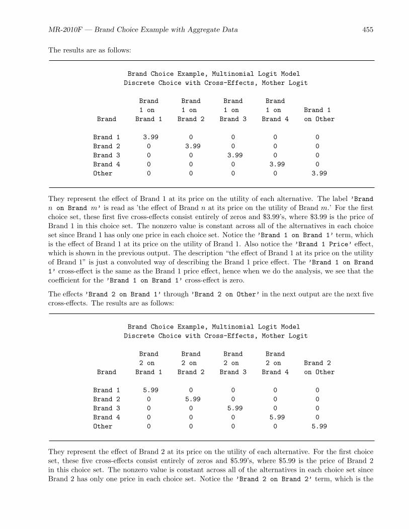
MR-2010F — Brand Choice Example with Aggregate Data 455
The results are as follows:
Brand Choice Example, Multinomial Logit ModelDiscrete Choice with Cross-Effects, Mother Logit
Brand Brand Brand Brand1 on 1 on 1 on 1 on Brand 1
Brand Brand 1 Brand 2 Brand 3 Brand 4 on Other
Brand 1 3.99 0 0 0 0Brand 2 0 3.99 0 0 0Brand 3 0 0 3.99 0 0Brand 4 0 0 0 3.99 0Other 0 0 0 0 3.99
They represent the effect of Brand 1 at its price on the utility of each alternative. The label ’Brandn on Brand m’ is read as ’the effect of Brand n at its price on the utility of Brand m.’ For the firstchoice set, these first five cross-effects consist entirely of zeros and $3.99’s, where $3.99 is the price ofBrand 1 in this choice set. The nonzero value is constant across all of the alternatives in each choiceset since Brand 1 has only one price in each choice set. Notice the ’Brand 1 on Brand 1’ term, whichis the effect of Brand 1 at its price on the utility of Brand 1. Also notice the ’Brand 1 Price’ effect,which is shown in the previous output. The description “the effect of Brand 1 at its price on the utilityof Brand 1” is just a convoluted way of describing the Brand 1 price effect. The ’Brand 1 on Brand1’ cross-effect is the same as the Brand 1 price effect, hence when we do the analysis, we see that thecoefficient for the ’Brand 1 on Brand 1’ cross-effect is zero.
The effects ’Brand 2 on Brand 1’ through ’Brand 2 on Other’ in the next output are the next fivecross-effects. The results are as follows:
Brand Choice Example, Multinomial Logit ModelDiscrete Choice with Cross-Effects, Mother Logit
Brand Brand Brand Brand2 on 2 on 2 on 2 on Brand 2
Brand Brand 1 Brand 2 Brand 3 Brand 4 on Other
Brand 1 5.99 0 0 0 0Brand 2 0 5.99 0 0 0Brand 3 0 0 5.99 0 0Brand 4 0 0 0 5.99 0Other 0 0 0 0 5.99
They represent the effect of Brand 2 at its price on the utility of each alternative. For the first choiceset, these five cross-effects consist entirely of zeros and $5.99’s, where $5.99 is the price of Brand 2in this choice set. The nonzero value is constant across all of the alternatives in each choice set sinceBrand 2 has only one price in each choice set. Notice the ’Brand 2 on Brand 2’ term, which is the

456 MR-2010F — Discrete Choice
effect of Brand 2 at its price on the utility of Brand 2. The description “the effect of Brand 2 at its priceon the utility of Brand 2” is just a convoluted way of describing the Brand 2 price effect. The ’Brand2 on Brand 2’ cross-effect is the same as the Brand 2 price effect, hence when we do the analysis, wesee that the coefficient for the ’Brand 2 on Brand 2’ cross-effect is zero.
The effects ’Brand 3 on Brand 1’ through ’Brand 3 on Other’ in the next output are the next fivecross-effects. The results are as follows:
Brand Choice Example, Multinomial Logit ModelDiscrete Choice with Cross-Effects, Mother Logit
Brand Brand Brand Brand3 on 3 on 3 on 3 on Brand 3
Brand Brand 1 Brand 2 Brand 3 Brand 4 on Other
Brand 1 3.99 0 0 0 0Brand 2 0 3.99 0 0 0Brand 3 0 0 3.99 0 0Brand 4 0 0 0 3.99 0Other 0 0 0 0 3.99
They represent the effect of Brand 3 at its price on the utility of each alternative. For the first choiceset, these five cross-effects consist entirely of zeros and $3.99’s, where $3.99 is the price of Brand 3 inthis choice set. Notice that the ’Brand 3 on Brand 3’ term is the same as the Brand 3 price effect,hence when we do the analysis, see that the coefficient for the ’Brand 3 on Brand 3’ cross-effect iszero.
The remaining cross-effects follow the same pattern that was described for the previous cross-effectsand are as follows:
Brand Choice Example, Multinomial Logit ModelDiscrete Choice with Cross-Effects, Mother Logit
Brand Brand Brand Brand4 on 4 on 4 on 4 on Brand 4
Brand Brand 1 Brand 2 Brand 3 Brand 4 on Other
Brand 1 5.99 0 0 0 0Brand 2 0 5.99 0 0 0Brand 3 0 0 5.99 0 0Brand 4 0 0 0 5.99 0Other 0 0 0 0 5.99

MR-2010F — Brand Choice Example with Aggregate Data 457
Brand Choice Example, Multinomial Logit ModelDiscrete Choice with Cross-Effects, Mother Logit
Other on Other on Other on Other on Other onBrand Brand 1 Brand 2 Brand 3 Brand 4 Other
Brand 1 4.99 0 0 0 0Brand 2 0 4.99 0 0 0Brand 3 0 0 4.99 0 0Brand 4 0 0 0 4.99 0Other 0 0 0 0 4.99
We have been describing variables by their labels. While it is not necessary to look at it, the & trgindmacro variable name list that PROC TRANSREG creates for this problem is as follows:
%put &_trgind;
BrandBrand_1 BrandBrand_2 BrandBrand_3 BrandBrand_4 BrandOtherBrandBrand_1Price BrandBrand_2Price BrandBrand_3Price BrandBrand_4PriceBrandOtherPrice p1BrandBrand_1 p1BrandBrand_2 p1BrandBrand_3 p1BrandBrand_4p1BrandOther p2BrandBrand_1 p2BrandBrand_2 p2BrandBrand_3 p2BrandBrand_4p2BrandOther p3BrandBrand_1 p3BrandBrand_2 p3BrandBrand_3 p3BrandBrand_4p3BrandOther p4BrandBrand_1 p4BrandBrand_2 p4BrandBrand_3 p4BrandBrand_4p4BrandOther p5BrandBrand_1 p5BrandBrand_2 p5BrandBrand_3 p5BrandBrand_4p5BrandOther
The analysis proceeds in exactly the same manner as before as follows:
proc phreg data=coded brief;model c*c(2) = &_trgind / ties=breslow;strata subj set;run;
The results are as follows:
Brand Choice Example, Multinomial Logit ModelDiscrete Choice with Cross-Effects, Mother Logit
The PHREG Procedure
Model Information
Data Set WORK.CODEDDependent Variable cCensoring Variable cCensoring Value(s) 2Ties Handling BRESLOW

458 MR-2010F — Discrete Choice
Number of Observations Read 4000Number of Observations Used 4000
Summary of Subjects, Sets, and Chosen and Unchosen Alternatives
Number of Number of Chosen NotPattern Choices Alternatives Alternatives Chosen
1 800 5 1 4
Convergence Status
Convergence criterion (GCONV=1E-8) satisfied.
Model Fit Statistics
Without WithCriterion Covariates Covariates
-2 LOG L 2575.101 2349.325AIC 2575.101 2389.325SBC 2575.101 2483.018
Testing Global Null Hypothesis: BETA=0
Test Chi-Square DF Pr > ChiSq
Likelihood Ratio 225.7752 20 <.0001Score 218.4500 20 <.0001Wald 190.0257 20 <.0001
Multinomial Logit Parameter Estimates
Parameter StandardDF Estimate Error Chi-Square Pr > ChiSq
Brand 1 1 1.24963 1.31259 0.9064 0.3411Brand 2 1 -0.16269 1.38579 0.0138 0.9065Brand 3 1 -3.90179 1.56511 6.2150 0.0127Brand 4 1 2.49435 1.25537 3.9480 0.0469Other 0 0 . . .Brand 1 Price 1 0.51056 0.13178 15.0096 0.0001Brand 2 Price 1 -0.04920 0.13411 0.1346 0.7137Brand 3 Price 1 -0.27594 0.15517 3.1623 0.0754Brand 4 Price 1 0.28951 0.12192 5.6389 0.0176Other Price 0 0 . . .Brand 1 on Brand 1 0 0 . . .Brand 1 on Brand 2 1 0.51651 0.13675 14.2653 0.0002Brand 1 on Brand 3 1 0.66122 0.15655 17.8397 <.0001Brand 1 on Brand 4 1 0.32806 0.12664 6.7105 0.0096Brand 1 on Other 0 0 . . .
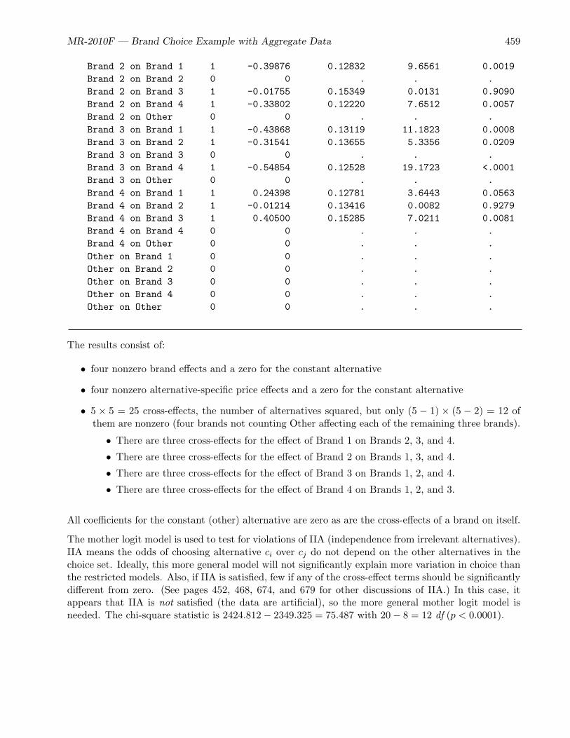
MR-2010F — Brand Choice Example with Aggregate Data 459
Brand 2 on Brand 1 1 -0.39876 0.12832 9.6561 0.0019Brand 2 on Brand 2 0 0 . . .Brand 2 on Brand 3 1 -0.01755 0.15349 0.0131 0.9090Brand 2 on Brand 4 1 -0.33802 0.12220 7.6512 0.0057Brand 2 on Other 0 0 . . .Brand 3 on Brand 1 1 -0.43868 0.13119 11.1823 0.0008Brand 3 on Brand 2 1 -0.31541 0.13655 5.3356 0.0209Brand 3 on Brand 3 0 0 . . .Brand 3 on Brand 4 1 -0.54854 0.12528 19.1723 <.0001Brand 3 on Other 0 0 . . .Brand 4 on Brand 1 1 0.24398 0.12781 3.6443 0.0563Brand 4 on Brand 2 1 -0.01214 0.13416 0.0082 0.9279Brand 4 on Brand 3 1 0.40500 0.15285 7.0211 0.0081Brand 4 on Brand 4 0 0 . . .Brand 4 on Other 0 0 . . .Other on Brand 1 0 0 . . .Other on Brand 2 0 0 . . .Other on Brand 3 0 0 . . .Other on Brand 4 0 0 . . .Other on Other 0 0 . . .
The results consist of:
• four nonzero brand effects and a zero for the constant alternative
• four nonzero alternative-specific price effects and a zero for the constant alternative
• 5 × 5 = 25 cross-effects, the number of alternatives squared, but only (5 − 1) × (5 − 2) = 12 ofthem are nonzero (four brands not counting Other affecting each of the remaining three brands).
• There are three cross-effects for the effect of Brand 1 on Brands 2, 3, and 4.
• There are three cross-effects for the effect of Brand 2 on Brands 1, 3, and 4.
• There are three cross-effects for the effect of Brand 3 on Brands 1, 2, and 4.
• There are three cross-effects for the effect of Brand 4 on Brands 1, 2, and 3.
All coefficients for the constant (other) alternative are zero as are the cross-effects of a brand on itself.
The mother logit model is used to test for violations of IIA (independence from irrelevant alternatives).IIA means the odds of choosing alternative ci over cj do not depend on the other alternatives in thechoice set. Ideally, this more general model will not significantly explain more variation in choice thanthe restricted models. Also, if IIA is satisfied, few if any of the cross-effect terms should be significantlydifferent from zero. (See pages 452, 468, 674, and 679 for other discussions of IIA.) In this case, itappears that IIA is not satisfied (the data are artificial), so the more general mother logit model isneeded. The chi-square statistic is 2424.812− 2349.325 = 75.487 with 20− 8 = 12 df (p < 0.0001).

460 MR-2010F — Discrete Choice
You could eliminate some of the zero parameters by changing zero=none to zero=’Other’ and elimi-nating p5 (p&m) from the model as follows:
proc transreg design data=price nozeroconstant norestoremissing;model class(brand / zero=’Other’ separators=’’ ’ ’) | identity(price)
identity(p1-p4) * class(brand / zero=’Other’ separators=’’ ’ on ’) /lprefix=0;
output out=coded(drop=_type_ _name_ intercept);label price = ’Price’
p1 = ’Brand 1’ p2 = ’Brand 2’ p3 = ’Brand 3’p4 = ’Brand 4’;
id subj set c;run;
You could also eliminate the brand by price effects and instead capture brand by price effects as thecross-effect of a variable on itself as follows:
proc transreg design data=price nozeroconstant norestoremissing;model class(brand / zero=’Other’ separators=’’ ’ ’)
identity(p1-p4) * class(brand / zero=’Other’ separators=’’ ’ on ’) /lprefix=0;
output out=coded(drop=_type_ _name_ intercept);label price = ’Price’
p1 = ’Brand 1’ p2 = ’Brand 2’ p3 = ’Brand 3’p4 = ’Brand 4’;
id subj set c;run;
In both cases, the analysis (not shown) is run in the usual manner. Except for the elimination of zeroterms, and in the second case, the change to capture the price effects in the cross-effects, the resultsare identical.
Aggregating the Data
In all examples so far (except the last part of the last vacation example), the data set has been createdfor analysis with one stratum for each choice set and subject combination. Such data sets can be large.The data can also be arrayed with a frequency variable and each choice set forming a separate stratum.The following example illustrates how:

MR-2010F — Brand Choice Example with Aggregate Data 461
title ’Brand Choice Example, Multinomial Logit Model’;title2 ’Aggregate Data’;
%let m = 5; /* Number of Brands in Each Choice Set *//* (including Other) */
proc format;value brand 1 = ’Brand 1’ 2 = ’Brand 2’ 3 = ’Brand 3’
4 = ’Brand 4’ 5 = ’Other’;run;
data price2;array p[&m] p1-p&m; /* Prices for the Brands */array f[&m] f1-f&m; /* Frequency of Choice */
input p1-p&m f1-f&m;keep set price brand freq c p1-p&m;
* Store choice set number to stratify;Set = _n_;
do Brand = 1 to &m;
Price = p[brand];
* Output first choice: c=1, unchosen: c=2;Freq = f[brand]; c = 1; output;
* Output number of times brand is not chosen.;freq = sum(of f1-f&m) - freq; c = 2; output;
end;
format brand brand.;
datalines;3.99 5.99 3.99 5.99 4.99 4 29 16 42 95.99 5.99 5.99 5.99 4.99 12 19 22 33 145.99 5.99 3.99 3.99 4.99 34 26 8 27 55.99 3.99 5.99 3.99 4.99 13 37 15 27 85.99 3.99 3.99 5.99 4.99 49 1 9 37 43.99 5.99 5.99 3.99 4.99 31 12 6 18 333.99 3.99 5.99 5.99 4.99 37 10 5 35 133.99 3.99 3.99 3.99 4.99 16 14 5 51 14;
proc print data=price2(obs=10);var set c freq price brand;run;

462 MR-2010F — Discrete Choice
The results are as follows:
Brand Choice Example, Multinomial Logit ModelAggregate Data
Obs Set c Freq Price Brand
1 1 1 4 3.99 Brand 12 1 2 96 3.99 Brand 13 1 1 29 5.99 Brand 24 1 2 71 5.99 Brand 25 1 1 16 3.99 Brand 36 1 2 84 3.99 Brand 37 1 1 42 5.99 Brand 48 1 2 58 5.99 Brand 49 1 1 9 4.99 Other10 1 2 91 4.99 Other
This data set has 5 brands times 2 observations times 8 choice sets for a total of 80 observations,compared to 100 × 5 × 8 = 4000 using the standard method. Two observations are created for eachalternative within each choice set. The first contains the number of people who chose the alternative,and the second contains the number of people who did not choose the alternative.
To analyze the data, specify strata Set and freq Freq. The following steps code and analyze thedata:
proc transreg design data=price2 nozeroconstant norestoremissing;model class(brand / zero=none) identity(price) / lprefix=0;output out=coded(drop=_type_ _name_ intercept);label price = ’Price’;id freq set c;run;
proc phreg data=coded;title2 ’Discrete Choice with Common Price Effect, Aggregate Data’;model c*c(2) = &_trgind / ties=breslow;strata set;freq freq;run;
These steps produced the following results:

MR-2010F — Brand Choice Example with Aggregate Data 463
Brand Choice Example, Multinomial Logit ModelDiscrete Choice with Common Price Effect, Aggregate Data
The PHREG Procedure
Model Information
Data Set WORK.CODEDDependent Variable cCensoring Variable cCensoring Value(s) 2Frequency Variable FreqTies Handling BRESLOW
Number of Observations Read 80Number of Observations Used 80Sum of Frequencies Read 4000Sum of Frequencies Used 4000
Summary of Subjects, Sets, and Chosen and Unchosen Alternatives
Number of Chosen NotStratum Set Alternatives Alternatives Chosen
1 1 500 100 4002 2 500 100 4003 3 500 100 4004 4 500 100 4005 5 500 100 4006 6 500 100 4007 7 500 100 4008 8 500 100 400
---------------------------------------------------------------Total 4000 800 3200
Convergence Status
Convergence criterion (GCONV=1E-8) satisfied.
Model Fit Statistics
Without WithCriterion Covariates Covariates
-2 LOG L 9943.373 9793.486AIC 9943.373 9803.486SBC 9943.373 9826.909

464 MR-2010F — Discrete Choice
Testing Global Null Hypothesis: BETA=0
Test Chi-Square DF Pr > ChiSq
Likelihood Ratio 149.8868 5 <.0001Score 153.2328 5 <.0001Wald 142.9002 5 <.0001
Multinomial Logit Parameter Estimates
Parameter StandardDF Estimate Error Chi-Square Pr > ChiSq
Brand 1 1 0.66727 0.12305 29.4065 <.0001Brand 2 1 0.38503 0.12962 8.8235 0.0030Brand 3 1 -0.15955 0.14725 1.1740 0.2786Brand 4 1 0.98964 0.11720 71.2993 <.0001Other 0 0 . . .Price 1 0.14966 0.04406 11.5379 0.0007
The summary table is small with eight rows, one row per choice set. Each row represents 100 chosenalternatives and 400 unchosen. The ’Analysis of Maximum Likelihood Estimates’ table exactly matchesthe one produced by the standard analysis. The –2 LOG L statistics are different than before: 9793.486now compared to 2425.214 previously. This is because the data are arrayed in this example so thatthe partial likelihood of the proportional hazards model fit by PROC PHREG with the ties=breslowoption is now proportional to—not identical to—the likelihood for the choice model. However, theModel Chi-Square statistics, df, and p-values are the same as before. The two corresponding pairs of –2LOG L’s differ by a constant 9943.373−2575.101 = 9793.486−2425.214 = 7368.272 = 2×800×log(100).Since the χ2 is the –2 LOG L without covariates minus –2 LOG L with covariates, the constants canceland the χ2 test is correct for both methods.
The technique of aggregating the data and using a frequency variable can be used for other models aswell, for example, with brand by price effects as follows:
proc transreg design data=price2 nozeroconstant norestoremissing;model class(brand / zero=none separators=’’ ’ ’) |
identity(price) / lprefix=0;output out=coded(drop=_type_ _name_ intercept);label price = ’Price’;id freq set c;run;
proc phreg data=coded;title2 ’Discrete Choice with Brand by Price Effects, Aggregate Data’;model c*c(2) = &_trgind / ties=breslow;strata set;freq freq;run;

MR-2010F — Brand Choice Example with Aggregate Data 465
This step produced the following results:
Brand Choice Example, Multinomial Logit ModelDiscrete Choice with Brand by Price Effects, Aggregate Data
The PHREG Procedure
Model Information
Data Set WORK.CODEDDependent Variable cCensoring Variable cCensoring Value(s) 2Frequency Variable FreqTies Handling BRESLOW
Number of Observations Read 80Number of Observations Used 80Sum of Frequencies Read 4000Sum of Frequencies Used 4000
Summary of Subjects, Sets, and Chosen and Unchosen Alternatives
Number of Chosen NotStratum Set Alternatives Alternatives Chosen
1 1 500 100 4002 2 500 100 4003 3 500 100 4004 4 500 100 4005 5 500 100 4006 6 500 100 4007 7 500 100 4008 8 500 100 400
---------------------------------------------------------------Total 4000 800 3200
Convergence Status
Convergence criterion (GCONV=1E-8) satisfied.
Model Fit Statistics
Without WithCriterion Covariates Covariates
-2 LOG L 9943.373 9793.084AIC 9943.373 9809.084SBC 9943.373 9846.561
466 MR-2010F — Discrete Choice
Testing Global Null Hypothesis: BETA=0
Test Chi-Square DF Pr > ChiSq
Likelihood Ratio 150.2891 8 <.0001Score 154.2562 8 <.0001Wald 143.1425 8 <.0001
Multinomial Logit Parameter Estimates
Parameter StandardDF Estimate Error Chi-Square Pr > ChiSq
Brand 1 1 -0.00972 0.43555 0.0005 0.9822Brand 2 1 -0.62230 0.48866 1.6217 0.2028Brand 3 1 -0.81250 0.60318 1.8145 0.1780Brand 4 1 0.31778 0.39549 0.6456 0.4217Other 0 0 . . .Brand 1 Price 1 0.13587 0.08259 2.7063 0.1000Brand 2 Price 1 0.20074 0.09210 4.7512 0.0293Brand 3 Price 1 0.13126 0.11487 1.3057 0.2532Brand 4 Price 1 0.13478 0.07504 3.2255 0.0725Other Price 0 0 . . .
The only thing that changes from the analysis with one stratum for each subject and choice setcombination is the likelihood.
Previously, with one stratum per choice set within subject, we compared these models as follows: “Thedifference 2425.214 − 2424.812 = 0.402 is distributed χ2 with 8 − 5 = 3 df and is not statisticallysignificant.” The difference between two −2 log(LC)’s equals the difference between two −2 log(LB)’s,since the constant terms (800× log(100)) cancel, 9793.486− 9793.084 = 2425.214− 2424.812 = 0.402.
Choice and Breslow Likelihood Comparison
This section explains why the –2 LOG L values differ by a constant with aggregate data versus individualdata. It can be skipped by all but the most dedicated readers.
Consider the choice model with a common price slope. Let x0 represent the price of the brand. Letx1, x2, x3, and x4 be indicator variables representing the choice of brands. Let x = (x0 x1 x2 x3 x4)be the vector of alternative attributes. (A sixth element for ’Other’ is omitted, since its parameter isalways zero given the other brands.)
Consider the first choice set. There are five distinct vectors of alternative attributesx1 = (3.99 1 0 0 0) x2 = (5.99 0 1 0 0) x3 = (3.99 0 0 1 0) x4 = (5.99 0 0 0 1)x5 = (4.99 0 0 0 0)

MR-2010F — Brand Choice Example with Aggregate Data 467
The vector x2, for example, represents choice of Brand 2, and x5 represents the choice of Other. Onehundred individuals are asked to choose one of the m = 5 brands from each of the eight sets. Let f1,f2, f3, f4, and f5 be the number of times each brand is chosen. For the first choice set, f1 = 4, f2 = 29,f3 = 16, f4 = 42, and f5 = 9. Let N be the total frequency for each choice set, N =
∑5j=1 fj = 100.
The likelihood LC1 for the first choice set data is
LC1 =
exp((∑5
j=1 fjxj
)β
)[∑5
j=1 exp(xjβ)]N
The joint likelihood for all eight choice sets is the product of the likelihoods
LC =8∏
k=1
LCk
The Breslow likelihood for this example, LBk , for the kth choice set, is the same as the likelihood for
the choice model, except for a multiplicative constant.
LCk = NNLB
k = 100100LBk
Therefore, the Breslow likelihood for all eight choice sets is
LB =8∏
k=1
LBk = N−8NLC = 100−800LC
The two likelihoods are not exactly the same, because each choice set is designated as a separatestratum, instead of each choice set within each subject.
The log likelihood for the choice model is
log(LC) = 800× log(100) + log(LB),log(LC) = 800× log(100) + (−0.5)× 9793.486,
log(LC) = −1212.607
and −2 log(LC) = 2425.214, which matches the earlier output. However, it is usually not necessary toobtain this value.
468 MR-2010F — Discrete Choice
Food Product Example with Asymmetry andAvailability Cross-Effects
This example is based on the choice example from page 255. This example discusses the multinomiallogit model, number of parameters, choosing the number of choice sets, designing the choice experiment,long design searches, examining the design, examining the subdesigns, examining the aliasing structure,blocking the design, testing the design before data collection, generating artificial data, processing thedata, coding, cross-effects, availability, multinomial logit model results, modeling subject attributes,results, and interpretation.
Consider the problem of using a discrete choice model to study the effect of introducing a retail foodproduct. This might be useful, for instance, to refine a marketing plan or to optimize a product priorto test market. A typical brand team has several concerns such as knowing the potential market sharefor the product, examining the source of volume, and providing guidance for pricing and promotions.The brand team might also want to know what brand attributes have competitive clout and want toidentify competitive attributes to which they are vulnerable.
To develop this further, assume our client wishes to introduce a line extension in the category of frozenentrees. The client has one nationally branded competitor, a regional competitor in each of threeregions, and a profusion of private label products at the grocery chain level. The product can comein two different forms: stove-top or microwaveable. The client believes that the private labels are verylikely to mimic this line extension and to sell it at a lower price. The client suspects that this strategyon the part of private labels might work for the stove-top version but not for the microwaveable, wherethey have the edge on perceived quality. They also want to test the effect of a shelf talker that drawsattention to their product.
The Multinomial Logit Model
This problem can be set up as a discrete choice model in which a respondent’s choice among brands,given choice set Ca of available brands, corresponds to the brand with the highest utility. For eachbrand i, the utility Ui is the sum of a systematic component Vi and a random component ei. Theprobability of choosing brand i from choice set Ca is therefore:
P (i|Ca) = P (Ui > max(Uj)) = P (Vi + ei > max(Vj + ej)) ∀ (j 6= i) ∈ Ca
Assuming that the ei follow an extreme value type I distribution, the conditional probabilities P (i|Ca)can be found using the multinomial logit (MNL) formulation of McFadden (1974).
P (i|Ca) = exp(Vi)/∑
j∈Caexp(Vj)
One of the consequences of the MNL formulation is the property of independence from irrelevantalternatives (IIA). Under the assumption of IIA, all cross-effects are assumed to be equal, so that ifa brand gains in utility, it draws share from all other brands in proportion to their current shares.Departures from IIA exist when certain subsets of brands are in more direct competition and tend todraw a disproportionate amount of share from each other than from other members in the category.

MR-2010F — Food Product Example with Asymmetry and Availability Cross-Effects 469
IIA is frequently described using a transportation example. Say you have three alternatives for gettingto work: bicycle, car, or a blue bus. If a fourth alternative became available, a red bus, then accordingto IIA the red bus should draw riders from the other alternatives in proportion to their current usage.However, in this case, IIA is violated, and instead the red bus draws more riders from the blue busthan from car drivers and bicycle riders.
The mother logit formulation of McFadden (1974) can be used to capture departures from IIA. Ina mother logit model, the utility for brand i is a function of both the attributes of brand i andthe attributes of other brands. The effect of one brand’s attributes on another is termed a cross-effect. In the case of designs in which only subsets Ca of the full shelf set C appear, the effect ofthe presence/absence of one brand on the utility of another is termed an availability cross-effect. (Seepages 452, 459, 674, and 679 for other discussions of IIA.)
Set Up
In the frozen entree example, there are five alternatives: the client’s brand, the client’s line extension, anational branded competitor, a regional brand and a private label brand. Several regional and privatelabels can be tested in each market, then aggregated for the final model. Note that the line extensionis treated as a separate alternative rather than as a level of the client brand. This enables us to modelthe source of volume for the new entry and to quantify any cannibalization that occurs. Each brandis shown at either two or three price points. Additional price points are included so that quadraticmodels of price elasticity can be tested. The indicator for the presence or absence of a brand in theshelf set is coded using one level of the Price variable. The layout of factors and levels is given in thefollowing table.
Factors and Levels
Alternative Factor Levels Brand Description1 X1 4 Client 1.29, 1.69, 2.09 + absent
2 X2 4 Client Line Extension 1.39, 1.89, 2.39, + absentX3 2 microwave/stove-topX4 2 shelf talker yes/no
3 X5 3 Regional 1.99, 2.49 + absent
4 X6 3 Private Label 1.49, 2.29 absentX7 2 microwave/stove-top
5 X8 3 National 1.99 + 2.39 + absent
In addition to intercepts and main effects, we also require that all two-way interactions within alter-natives be estimable: x2*x3, x2*x4, x3*x4 for the line extension and x6*x7 for private labels. Thisenables us to test for different price elasticities by form (stove-top versus microwaveable) and to see ifthe promotion works better combined with a low price or with different forms. Using a linear modelfor x1-x8, the total number of parameters including the intercept, all main effects, and two-way in-teractions with brand is 25. This assumes that price is treated as qualitative. The actual number ofparameters in the choice model is larger than this because of the inclusion of cross-effects.
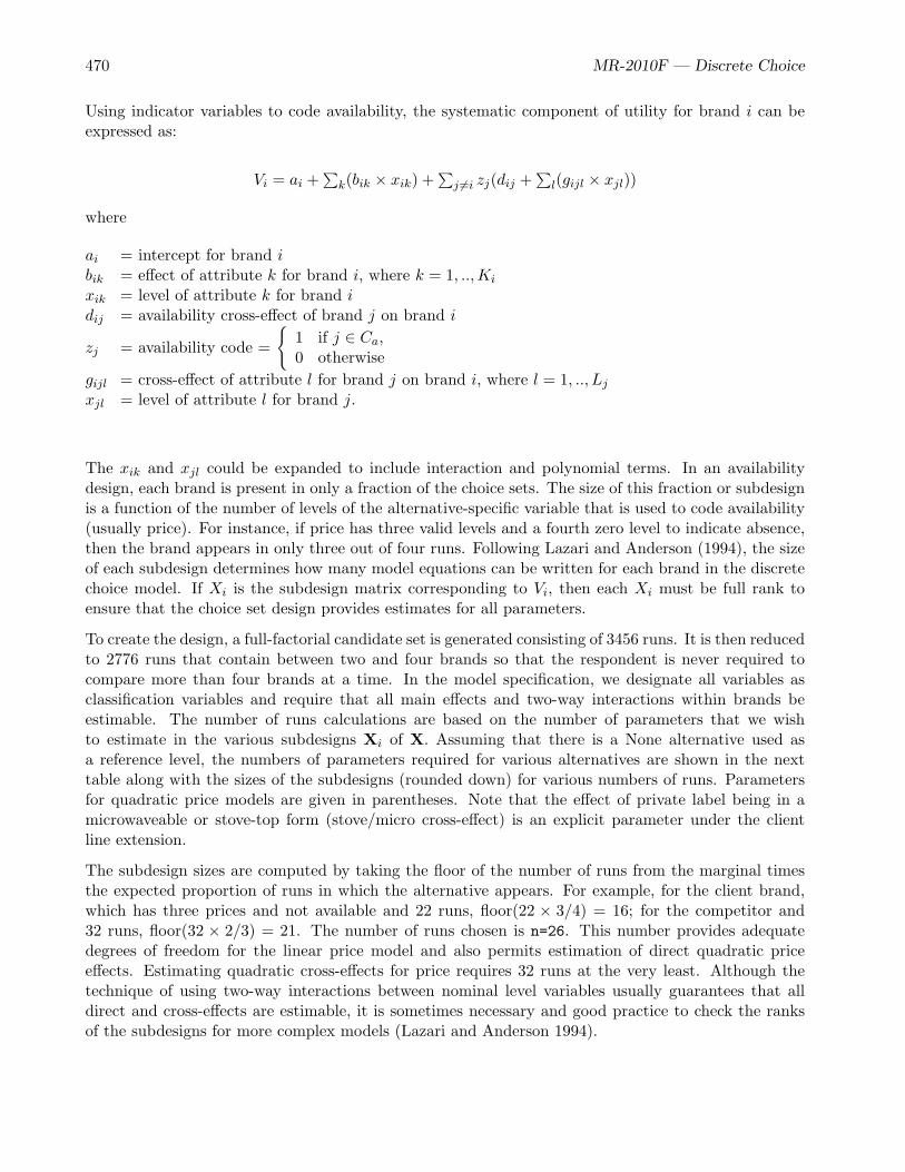
470 MR-2010F — Discrete Choice
Using indicator variables to code availability, the systematic component of utility for brand i can beexpressed as:
Vi = ai +∑
k(bik × xik) +∑
j 6=i zj(dij +∑
l(gijl × xjl))
where
ai = intercept for brand ibik = effect of attribute k for brand i, where k = 1, ..,Ki
xik = level of attribute k for brand idij = availability cross-effect of brand j on brand i
zj = availability code =
{1 if j ∈ Ca,0 otherwise
gijl = cross-effect of attribute l for brand j on brand i, where l = 1, .., Lj
xjl = level of attribute l for brand j.
The xik and xjl could be expanded to include interaction and polynomial terms. In an availabilitydesign, each brand is present in only a fraction of the choice sets. The size of this fraction or subdesignis a function of the number of levels of the alternative-specific variable that is used to code availability(usually price). For instance, if price has three valid levels and a fourth zero level to indicate absence,then the brand appears in only three out of four runs. Following Lazari and Anderson (1994), the sizeof each subdesign determines how many model equations can be written for each brand in the discretechoice model. If Xi is the subdesign matrix corresponding to Vi, then each Xi must be full rank toensure that the choice set design provides estimates for all parameters.
To create the design, a full-factorial candidate set is generated consisting of 3456 runs. It is then reducedto 2776 runs that contain between two and four brands so that the respondent is never required tocompare more than four brands at a time. In the model specification, we designate all variables asclassification variables and require that all main effects and two-way interactions within brands beestimable. The number of runs calculations are based on the number of parameters that we wishto estimate in the various subdesigns Xi of X. Assuming that there is a None alternative used asa reference level, the numbers of parameters required for various alternatives are shown in the nexttable along with the sizes of the subdesigns (rounded down) for various numbers of runs. Parametersfor quadratic price models are given in parentheses. Note that the effect of private label being in amicrowaveable or stove-top form (stove/micro cross-effect) is an explicit parameter under the clientline extension.
The subdesign sizes are computed by taking the floor of the number of runs from the marginal timesthe expected proportion of runs in which the alternative appears. For example, for the client brand,which has three prices and not available and 22 runs, floor(22 × 3/4) = 16; for the competitor and32 runs, floor(32 × 2/3) = 21. The number of runs chosen is n=26. This number provides adequatedegrees of freedom for the linear price model and also permits estimation of direct quadratic priceeffects. Estimating quadratic cross-effects for price requires 32 runs at the very least. Although thetechnique of using two-way interactions between nominal level variables usually guarantees that alldirect and cross-effects are estimable, it is sometimes necessary and good practice to check the ranksof the subdesigns for more complex models (Lazari and Anderson 1994).

MR-2010F — Food Product Example with Asymmetry and Availability Cross-Effects 471
ParametersClient Private
Effect Client Line Extension Regional Label Competitorintercept 1 1 1 1 1availability cross-effects 4 4 4 4 4direct price effect 1 (2) 1 (2) 1 1 1price cross-effects 4 (8) 4 (8) 4 4 4stove versus microwave - 1 - 1 -stove/micro cross-effects - 1 - - -shelf talker - 1 - - -price*stove/microwave - 1 (2) - 1 -price*shelf talker - 1 (2) - - -stove/micro*shelf talker - 1 - - -
Total 10 (15) 16 (23) 10 12 10
Subdesign size
22 runs 16 16 14 14 1426 runs 19 19 17 17 1732 runs 24 24 21 21 21
Designing the Choice Experiment
This example originated with Kuhfeld, Tobias, and Garratt (1994), long before the %MktRuns macroexisted. At least for now, we will skip the customary step of running the %MktRuns macro to suggesta design size and instead use the original size of 26 choice sets.
We use the %MktEx autocall macro to create the design. (All of the autocall macros used in this bookare documented starting on page 803.) To recap, we want to make the design 233342 in 26 runs, andwe want the following interactions to be estimable: x2*x3 x2*x4 x3*x4 x6*x7. Furthermore, thereare restrictions on the design. Each of the price variables, x1, x2, x5, x6, and x8, has one level—themaximum level—that indicates the alternative is not available in the choice set. We use this to createchoice sets with 2, 3, or 4 alternatives available. If (x1 < 4) then the first alternative is available, if(x2 < 4) then the second alternative is available, if (x5 < 3) then the third alternative is available,and so on. A Boolean term such as (x1 < 4) is one when true and zero otherwise. Hence,
((x1 < 4) + (x2 < 4) + (x5 < 3) + (x6 < 3) + (x8 < 3))
is the number of available alternatives. It is simply the sum of some 1’s if available and 0’s if notavailable.
We impose restrictions with the %MktEx macro by writing a macro, with IML statements, that quantifiesthe badness of each run (or in this case, each choice set). We do this so bad = 0 is good and valueslarger than zero are increasingly worse. We write our restrictions using an IML row vector x thatcontains the levels (integers beginning with 1) of each of the factors in the ith choice set, the one themacro is currently seeking to improve. The jth factor is x[j], or we can also use the factor names (forexample, x1, x2). (See pages 604 and 1079 for other examples of restrictions.)

472 MR-2010F — Discrete Choice
We must use IML logical operators, which do not have all of the same syntactical alternatives as DATAstep operators:
Do NotSpecify For Specify= equals EQ∧ = or ¬ = not equals NE< less than LT<= less than or equal to LE> greater than GT>= greater than or equal to GE& and AND| or OR∧ or ¬ not NOTa <= b & b <= c range check a <= b <= c
To restrict the design, we must specify restrictions=macro-name, in this case restrictions=resmac,that names the macro that quantifies badness. The first statement counts up the number of availablealternatives. The next two set the actual badness value. Note that the else bad = 0 statement is notnecessary since bad is automatically initialized to zero by the %MktEx macro. If the number availableis less than two or greater than 4, then bad gets set to the absolute difference between the numberavailable and 3. Hence, zero available corresponds to bad = 3, one available corresponds to bad = 2,two through four available corresponds to bad = 0, and five available corresponds to bad = 2. Donot just set bad to zero when everything is fine and one otherwise, because the macro needs to knowthat when it switches from zero available to one available, it is going in the right direction. For simplerestrictions like this, it does not matter very much. However, for complicated sets of restrictions, itis critical that the bad variable is set to a count of the number of current restriction violations. Thefollowing steps create the design:∗
title ’Consumer Food Product Example’;
%macro resmac;navail = (x1 < 4) + (x2 < 4) + (x5 < 3) + (x6 < 3) + (x8 < 3);if (navail < 2) | (navail > 4) then bad = abs(navail - 3);else bad = 0;%mend;
%mktex(4 4 2 2 3 3 2 3, /* all attrs of all alternatives */n=26, /* number of choice sets */interact=x2*x3 x2*x4 x3*x4 x6*x7, /* interactions */restrictions=resmac, /* name of restrictions macro */seed=377, /* random number seed */outr=sasuser.EntreeLinDes1) /* randomized design stored permanently */
∗Due to machine, SAS release, and macro differences, you might not get exactly the same design used in this book,but the differences should be slight.
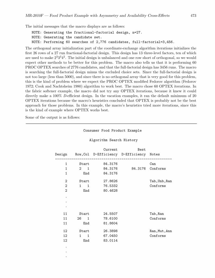
MR-2010F — Food Product Example with Asymmetry and Availability Cross-Effects 473
The initial messages that the macro displays are as follows:
NOTE: Generating the fractional-factorial design, n=27.NOTE: Generating the candidate set.NOTE: Performing 60 searches of 2,776 candidates, full-factorial=3,456.
The orthogonal array initialization part of the coordinate-exchange algorithm iterations initializes thefirst 26 rows of a 27 run fractional-factorial design. This design has 13 three-level factors, ten of whichare used to make 233342. The initial design is unbalanced and one row short of orthogonal, so we wouldexpect other methods to be better for this problem. The macro also tells us that it is performing 60PROC OPTEX searches of 2776 candidates, and that the full-factorial design has 3456 runs. The macrois searching the full-factorial design minus the excluded choice sets. Since the full-factorial design isnot too large (less than 5000), and since there is no orthogonal array that is very good for this problem,this is the kind of problem where we expect the PROC OPTEX modified Fedorov algorithm (Fedorov1972; Cook and Nachtsheim 1980) algorithm to work best. The macro chose 60 OPTEX iterations. Inthe fabric softener example, the macro did not try any OPTEX iterations, because it knew it coulddirectly make a 100% D-efficient design. In the vacation examples, it ran the default minimum of 20OPTEX iterations because the macro’s heuristics concluded that OPTEX is probably not be the bestapproach for those problems. In this example, the macro’s heuristics tried more iterations, since thisis the kind of example where OPTEX works best.
Some of the output is as follows:
Consumer Food Product Example
Algorithm Search History
Current BestDesign Row,Col D-Efficiency D-Efficiency Notes----------------------------------------------------------
1 Start 84.3176 Can1 2 1 84.3176 84.3176 Conforms1 End 84.3176
2 Start 27.8626 Tab,Unb,Ran2 1 1 76.5332 Conforms2 End 80.4628
.
.
.
11 Start 24.5507 Tab,Ran11 26 1 78.6100 Conforms11 End 81.8604
12 Start 26.3898 Ran,Mut,Ann12 1 1 67.0450 Conforms12 End 83.0114
.
.
.

474 MR-2010F — Discrete Choice
21 Start 45.9310 Ran,Mut,Ann21 15 1 67.1046 Conforms21 End 82.1657
NOTE: Performing 600 searches of 2,776 candidates.
Consumer Food Product Example
Design Search History
Current BestDesign Row,Col D-Efficiency D-Efficiency Notes----------------------------------------------------------
0 Initial 84.3176 84.3176 Ini
1 Start 84.7548 Can1 2 1 84.7548 84.7548 Conforms1 End 84.7548
Consumer Food Product Example
Design Refinement History
Current BestDesign Row,Col D-Efficiency D-Efficiency Notes----------------------------------------------------------
0 Initial 84.7548 84.7548 Ini
1 Start 84.7548 Pre,Mut,Ann1 2 1 82.6737 Conforms1 14 1 84.7548 84.75481 End 82.6386
.
.
.
8 Start 84.7548 Pre,Mut,Ann8 2 1 84.7548 84.7548 Conforms8 14 1 84.7548 84.75488 21 2 84.7548 84.75488 12 3 84.7548 84.75488 12 6 84.7548 84.75488 18 1 84.7548 84.75488 2 2 84.7548 84.75488 End 84.7548
NOTE: Stopping since it appears that no improvement is possible.
MR-2010F — Food Product Example with Asymmetry and Availability Cross-Effects 475
Consumer Food Product Example
The OPTEX Procedure
Class Level Information
Class Levels -Values-
x1 4 1 2 3 4x2 4 1 2 3 4x3 2 1 2x4 2 1 2x5 3 1 2 3x6 3 1 2 3x7 2 1 2
Consumer Food Product Example
The OPTEX Procedure
AveragePrediction
Design StandardNumber D-Efficiency A-Efficiency G-Efficiency Error------------------------------------------------------------------------
1 84.7548 71.1686 98.0583 0.9806
Design 1 (Can), which is created by the candidate-set search (using PROC OPTEX), has D-efficiencyor 84.3176, and the macro confirms that the design conforms to our restrictions. The orthogonal array,unbalanced, and random initializations do not work as well. For each design, the macro iteration historystates the D-efficiency for the initial design (27.8626 in design 2), the D-efficiency when the restrictionsare met (76.5332, Conforms), and the D-efficiency for the final design (80.4628). The fully-randominitialization tends to work a little better than the orthogonal array initialization for this problem, butnot as well as PROC OPTEX. At the end of the algorithm search phase, the macro decides to usePROC OPTEX and performs 600 more searches, and it finds a design with 84.7548% D-efficiency. Thedesign refinement step fails to improve on the best design. This step took 3.5 minutes.
Restrictions Formulated Using Actual Attribute Names and Levels
In the previous section, we constructed a macro to create a design, maximizing efficiency while forcingthe design to conform to a set of restrictions. We provide %MktEx with a macro that it used to evaluatehow well it is doing in imposing the restrictions. Internally, %MktEx stores its results in matrices,vectors, and scalars, with fixed names: x1, x2, x3, and so on. Levels of the factors are always positiveintegers starting with one. In practice, before you actually use the design, you will usually want tochange these names and levels to something else that is more meaningful to your particular problem. Insome cases, it might be more convenient to express your restrictions in terms of these more meaningfulnames and levels as well. To do that, you need to convert the %MktEx names and levels into your names
476 MR-2010F — Discrete Choice
and levels, for example, as follows:
%macro resmac;client = {1.29 1.69 2.09 .}[x1];extension = {1.39 1.89 2.39 .}[x2];regional = {1.99 2.49 .}[x5];private = {1.49 2.29 .}[x6];national = {1.99 2.39 .}[x8];
navail = (client ^= .) + (extension ^= .) + (regional ^= .) +(private ^= .) + (national ^= .);
if (navail < 2) | (navail > 4) then bad = abs(navail - 3);else bad = 0;%mend;
The first line creates a scalar called client, that has one of four values: 1.29 when x1 is 1, 1.69 whenx1 is 2, 2.09 when x1 is 3, and . (missing) when x1 is 4. Each of the first five assignment statementsuses the %MktEx factor variables as an index into a constant vector of levels and stores the result inthe attribute name so that restrictions can be posed in terms of the actual design problem. A literalvector consists of { list } and you can provide a subscript variable to index any vector, including aliteral vector by specifying [ variable ]. Hence, the first five statements just convert x1, x2, x5, x6,and x8 into names and levels that are familiar to the problem. Character vectors are allowed as well.The following step shows an alternative but equivalent formulation of the macro, treating the first twofactors as numeric and the rest as character:
%macro resmac;client = {1.29 1.69 2.09 .}[x1];extension = {1.39 1.89 2.39 .}[x2];regional = {"$1.99" "$2.49" "NA"}[x5];private = {"$1.49" "$2.29" "NA"}[x6];national = {"$1.99" "$2.39" "NA"}[x8];
navail = (client ^= .) + (extension ^= .) + (regional ^= "NA") +(private ^= "NA") + (national ^= "NA");
if (navail < 2) | (navail > 4) then bad = abs(navail - 3);else bad = 0;%mend;
You cannot mix quoted character strings and unquoted numbers within a vector, however you can putany value in quotes. There is one extremely important caveat. Several names are used internally by%MktEx , and are available for you to look at when writing your restrictions. You must not changethem. Do not use any of these names as names of anything you create when you write restrictionsmacros: i, try, x, x1 x2 ..., j1 j2 ..., xmat, pbad, bbad.
Macros like this are always be less efficient than macros based on the internal names since extraassignments are needed and the statements in the macro are evaluated many times. However, theslight loss of computer efficiency might be more than offset by the convenience of avoiding convertingyour restrictions to use internal names. It might not matter much for a problem such as this, but forcomplicated restrictions, it might be much easier to work with more informative names and levels. Youcan make the macro slightly more efficient, at a cost of a slightly more complicated looking restrictions

MR-2010F — Food Product Example with Asymmetry and Availability Cross-Effects 477
macro, by using options=nox to suppress the creation of x1, x2, and so on, and instead make themnemonic names and levels directly based on x. The macro must be changed, substituting x[1] forx1, x[2] for x2, and so on, as follows:
%macro resmac;client = {1.29 1.69 2.09 .}[x[1]];extension = {1.39 1.89 2.39 .}[x[2]];regional = {"$1.99" "$2.49" "NA"}[x[5]];private = {"$1.49" "$2.29" "NA"}[x[6]];national = {"$1.99" "$2.39" "NA"}[x[8]];
navail = (client ^= .) + (extension ^= .) + (regional ^= "NA") +(private ^= "NA") + (national ^= "NA");
if (navail < 2) | (navail > 4) then bad = abs(navail - 3);else bad = 0;%mend;
%mktex(4 4 2 2 3 3 2 3, /* all attrs of all alternatives */n=26, /* number of choice sets */interact=x2*x3 x2*x4 x3*x4 x6*x7, /* interactions */optiter=0, /* no PROC OPTEX iterations */tabiter=0, /* no OA initialization iterations */maxdesigns=10, /* make at most 10 designs */options=nox, /* suppress x1, x2, ... creation */restrictions=resmac, /* name of restrictions macro */seed=377) /* random number seed */
When You Have a Long Time to Search for an Efficient Design
With a moderate sized candidate set such as this one (2000 to 6000 runs), we might be able to dobetter with more iterations. To test this, PROC OPTEX was run 10,000 times over the winter holidayvacation, from December 22 through January 2, creating a total of 200,000 designs, 20 designs on eachtry. (This was many years ago on computers that were much slower than the ones we have today.) Thefollowing table provides a summary of the results:
PROCOPTEX Percent
Run D-Efficiency Improvement1 83.89592 83.9890 0.11%3 84.3763 0.46%6 84.7548 0.45%
84 85.1561 0.47%1535 85.3298 0.20%9576 85.3985 0.08%

478 MR-2010F — Discrete Choice
This example is interesting, because it shows the diminishing value of increasing the number of it-erations. Six minutes into the search, in the first six passes through PROC OPTEX (6 × 20 = 120total iterations), we found a design with reasonably good D-efficiency=84.7548. Over an hour intothe search, with (84 − 6) × 20 = 1560 more iterations, we get a small 0.47% increase in D-efficiencyto 85.1561. About one day into the search, with (1535 − 84) × 20 = 29, 020 more iterations, we getanother small 0.20% increase in D-efficiency, 85.3298. Finally, almost a week into the search, with(9576 − 1535) × 20 = 160, 820 more iterations, we get another small 0.08% increase in D-efficiency to85.3985. Our overall improvement over the best design found in 120 iterations was 0.75952%, aboutthree-quarters of a percent. These numbers will change with other problems and other seeds. However,as these results show, usually the first few iterations give you a good, efficient design, and usually,subsequent iterations give you slight improvements but with a cost of much greater run times. Next,we construct a plot of this table as follows:
data e;input n e;label n = ’PROC OPTEX Run’ e = ’D-Efficiency’;datalines;1 83.89592 83.98903 84.37636 84.754884 85.1561
1535 85.32989576 85.3985;
proc sgplot data=e;title ’Consumer Food Product Example’;title2 ’Maximum D-Efficiency Found Over Time’;series y=e x=n;yaxis values=(0 to 100 by 25);run;
The plot of maximum D-efficiency as a function of PROC OPTEX run number clearly shows that thegain in D-efficiency that comes from a large number of iterations is very slight.
MR-2010F — Food Product Example with Asymmetry and Availability Cross-Effects 479
If you have a lot of time to search for a good design, you can specify some of the time and maximumnumber of iteration parameters. Sometimes you might get lucky and find a better design. In this nextexample, maxtime=300 300 60 is specified. This gives the macro up to 300 minutes for the algorithmsearch step, 300 minutes for the design search step, and 60 minutes for the refinement step. The optionmaxiter= increases the number iterations to 10000 for each of the three steps (or the maximum time).With this specification, you expect the macro to run overnight. See the macro documentation (startingon page 1017) for more iteration options. Note that you must increase the number of iterations andthe maximum amount of time if you want the macro to run longer. With this specification, the macroperforms 1800 OPTEX iterations initially (compared to 60 by default). The following steps create therestrictions macro and search for a design:

480 MR-2010F — Discrete Choice
title ’Consumer Food Product Example’;
%macro resmac;navail = (x1 < 4) + (x2 < 4) + (x5 < 3) + (x6 < 3) + (x8 < 3);if (navail < 2) | (navail > 4) then bad = abs(navail - 3);else bad = 0;%mend;
%mktex(4 4 2 2 3 3 2 3, /* all attrs of all alternatives */n=26, /* number of choice sets */interact=x2*x3 x2*x4 x3*x4 x6*x7, /* interactions */restrictions=resmac, /* name of restrictions macro */seed=151, /* random number seed */maxtime=300 300 60, /* max time for each major search phase */maxiter=10000) /* max iterations for each phase */
The results from this step are not shown.
Examining the Design
We can use the %MktEval macro to start to evaluate the design as follows:
%mkteval(data=sasuser.EntreeLinDes1)
The results are as follows:
Consumer Food Product ExampleCanonical Correlations Between the Factors
There are 4 Canonical Correlations Greater Than 0.316
x1 x2 x3 x4 x5 x6 x7 x8
x1 1 0.30 0.20 0.11 0.42 0.26 0.09 0.33x2 0.30 1 0.10 0.10 0.13 0.17 0.51 0.18x3 0.20 0.10 1 0.08 0.09 0.30 0 0.10x4 0.11 0.10 0.08 1 0.09 0.10 0 0.10x5 0.42 0.13 0.09 0.09 1 0.24 0.05 0.43x6 0.26 0.17 0.30 0.10 0.24 1 0.14 0.13x7 0.09 0.51 0 0 0.05 0.14 1 0.14x8 0.33 0.18 0.10 0.10 0.43 0.13 0.14 1
MR-2010F — Food Product Example with Asymmetry and Availability Cross-Effects 481
Consumer Food Product ExampleCanonical Correlations > 0.316 Between the Factors
There are 4 Canonical Correlations Greater Than 0.316
r r Square
x2 x7 0.51 0.26x5 x8 0.43 0.18x1 x5 0.42 0.18x1 x8 0.33 0.11
Consumer Food Product ExampleSummary of Frequencies
There are 4 Canonical Correlations Greater Than 0.316* - Indicates Unequal Frequencies
Frequencies
* x1 7 8 6 5* x2 6 7 7 6
x3 13 13x4 13 13
* x5 9 8 9* x6 7 10 9* x7 12 14* x8 7 9 10* x1 x2 2 2 1 2 2 2 2 2 1 1 2 2 1 2 2 0* x1 x3 3 4 4 4 4 2 2 3* x1 x4 4 3 4 4 3 3 2 3* x1 x5 4 2 1 2 1 5 2 2 2 1 3 1* x1 x6 2 3 2 2 4 2 2 1 3 1 2 2* x1 x7 3 4 4 4 3 3 2 3* x1 x8 1 2 4 2 4 2 2 1 3 2 2 1* x2 x3 3 3 3 4 4 3 3 3* x2 x4 3 3 3 4 4 3 3 3* x2 x5 2 2 2 3 2 2 2 2 3 2 2 2* x2 x6 2 2 2 2 3 2 2 2 3 1 3 2* x2 x7 1 5 4 3 2 5 5 1* x2 x8 2 2 2 1 3 3 2 2 3 2 2 2* x3 x4 7 6 6 7* x3 x5 5 4 4 4 4 5* x3 x6 2 5 6 5 5 3* x3 x7 6 7 6 7* x3 x8 4 4 5 3 5 5* x4 x5 4 4 5 5 4 4* x4 x6 4 5 4 3 5 5* x4 x7 6 7 6 7* x4 x8 4 4 5 3 5 5
482 MR-2010F — Discrete Choice
* x5 x6 2 4 3 2 2 4 3 4 2* x5 x7 4 5 4 4 4 5* x5 x8 1 2 6 4 2 2 2 5 2* x6 x7 3 4 4 6 5 4* x6 x8 2 2 3 2 4 4 3 3 3* x7 x8 4 4 4 3 5 6
N-Way 1 1 1 1 1 1 1 1 1 1 1 1 1 1 1 1 1 1 11 1 1 1 1 1 1
Some of the canonical correlations are bigger than we would like. They all involve attributes indifferent alternatives, so they should not pose huge problems. Still, they are large enough to makesome researchers uncomfortable. The frequencies are pretty close to balanced. Perfect balance is notpossible with 26 choice sets and this design. If we are willing to consider blocking the design, we mightdo better with more choice sets.
Designing the Choice Experiment, More Choice Sets
Let’s run the %MktRuns macro to see what design size looks good. For now, we ignore the interactionsand just specify main effects as follows:
%mktruns(4 4 2 2 3 3 2 3)
The results are as follows:
Consumer Food Product Example
Design Summary
Number ofLevels Frequency
2 33 34 2
Consumer Food Product Example
Saturated = 16Full Factorial = 3,456

MR-2010F — Food Product Example with Asymmetry and Availability Cross-Effects 483
Some Reasonable Cannot BeDesign Sizes Violations Divided By
144 * 072 1 1648 3 996 3 9192 3 924 4 9 16120 4 9 16168 4 9 1636 7 8 16108 7 8 1616 S 21 3 6 9 12
* - 100% Efficient design can be made with the MktEx macro.
S - Saturated Design - The smallest design that can be made.Note that the saturated design is not one of therecommended designs for this problem. It is shownto provide some context for the recommended sizes.
n Design Reference
144 2 **118 3 ** 4 4 ** 2 Orthogonal Array144 2 **115 3 ** 4 4 ** 3 Orthogonal Array144 2 **113 3 ** 12 4 ** 2 Orthogonal Array144 2 **112 3 ** 8 4 ** 2 6 ** 1 Orthogonal Array144 2 **112 3 ** 4 4 ** 4 Orthogonal Array144 2 **111 3 ** 4 4 ** 2 6 ** 2 Orthogonal Array144 2 **110 3 ** 12 4 ** 3 Orthogonal Array
.
.
.
The smallest suggestion larger than 26 is 36. With this mix of factor levels, we would need 144 runs toget an orthogonal design (ignoring interactions), so we definitely want to stick with a nonorthogonaldesign. Balance is possible in 36 runs, but 36 cannot be divided by 2× 4 = 8 and 4× 4 = 16. With 36runs, a blocking factor is required (2 blocks of 18 or 3 blocks of 12). We would like the shelf talker toappear in half of the choice sets within block, so with two blocks, we want the number of choice setsto be divisible by 2× 2 = 4, and 36 can be divided by 4. Now let’s specify the interactions as follows:
%mktruns(4 4 2 2 3 3 2 3, interact=x2*x3 x2*x4 x3*x4 x6*x7)
484 MR-2010F — Discrete Choice
The results are as follows:
Consumer Food Product Example
Design Summary
Number ofLevels Frequency
2 33 34 2
Consumer Food Product Example
Saturated = 25Full Factorial = 3,456
Some Reasonable Cannot BeDesign Sizes Violations Divided By
144 2 3296 5 9 18192 5 9 1848 7 9 18 3272 9 16 32 48216 9 16 32 48120 14 9 16 18 32 48168 14 9 16 18 32 4836 25 8 16 24 32 48108 25 8 16 24 32 4825 S 61 2 3 4 6 8 9 12 16 18 24 32 48
S - Saturated Design - The smallest design that can be made.Note that the saturated design is not one of therecommended designs for this problem. It is shownto provide some context for the recommended sizes.
Thirty-six runs is still in our list of possibilities, but now we see that not only can it not be divided by8 and 16, it also cannot be divided by 24, 32, 48. We will try making a design in 36 runs and see howit looks.
In the previous try in 26 runs, the PROC OPTEX modified Fedorov algorithm worked best. Thereare two reasons why this probably happened. First, the full-factorial design is small enough to useas a candidate set. After imposing restrictions, the candidate set has 2,776 runs, and any size under5000 or 10,000 is very manageable. Second, the design has interactions. The coordinate exchangealgorithm by default considers only a single factor at a time, which is just one part of an interactionterm. Modified Fedorov in contrast, considers exchanges involving all of the factors. For this problem,Modified Fedorov is invariably superior to the default coordinate-exchange algorithm. However, we can

MR-2010F — Food Product Example with Asymmetry and Availability Cross-Effects 485
make coordinate exchange better, by having it perform multiple-column exchanges taking into accountthe interactions, just as we did in the vacation example on page 417. We use the order=matrix=SAS-data-set approach to looping over the columns of the design with the coordinate-exchange algorithm. Inthis case, coordinate exchange pairs columns 1, 5, and 8 with a randomly chosen column, it considersevery possible triple in columns 2, 3, and 4, and it pairs columns 6 and 7 with a randomly chosencolumn. The following steps generate the order matrix and search for a design:
title ’Consumer Food Product Example’;
%macro resmac;navail = (x1 < 4) + (x2 < 4) + (x5 < 3) + (x6 < 3) + (x8 < 3);if (navail < 2) | (navail > 4) then bad = abs(navail - 3);else bad = 0;%mend;
data mat;input a b c;datalines;
1 1 .2 3 45 5 .6 7 .8 8 .;
%mktex(4 4 2 2 3 3 2 3, /* all attrs of all alternatives */n=36, /* number of choice sets */order=matrix=mat, /* pairs/trips of cols to work on */interact=x2*x3 x2*x4 x3*x4 x6*x7, /* interactions */restrictions=resmac, /* name of restrictions macro */seed=377, /* random number seed */outr=sasuser.EntreeLinDes2) /* randomized design stored permanently */
%mkteval(data=sasuser.EntreeLinDes2)
A small part of the output from the %MktEx macro is as follows:
Consumer Food Product Example 1
Algorithm Search History
Current BestDesign Row,Col D-Efficiency D-Efficiency Notes----------------------------------------------------------
1 Start 94.0517 Can1 2 1 94.0517 94.0517 Conforms1 End 94.0517
.
.
.
486 MR-2010F — Discrete Choice
12 Start 71.6955 Ran,Mut,Ann12 1 1 78.5418 Conforms12 30 5 94.1433 94.143312 33 5 94.1507 94.150712 31 1 94.1532 94.153212 23 6 94.1553 94.155312 End 94.1553
Design Search History
Current BestDesign Row,Col D-Efficiency D-Efficiency Notes----------------------------------------------------------
0 Initial 94.1553 94.1553 Ini
.
.
.
3 Start 68.5288 Ran,Mut,Ann3 29 1 75.9029 Conforms3 22 5 94.1682 94.16823 34 5 94.1683 94.16833 35 6 94.2926 94.29263 16 8 94.3718 94.37183 24 6 94.3718 94.37183 9 1 94.4572 94.45723 End 94.2846
.
.
.
Consumer Food Product Example
The OPTEX Procedure
AveragePrediction
Design StandardNumber D-Efficiency A-Efficiency G-Efficiency Error------------------------------------------------------------------------
1 94.4571 88.7104 94.0740 0.8333
The order=matrix= option apparently helped. The coordinate exchange algorithm is in fact chosenover the modified Fedorov algorithm.
D-efficiency at 94.46% looks good. Part of the %MktEval results are as follows:

MR-2010F — Food Product Example with Asymmetry and Availability Cross-Effects 487
Consumer Food Product ExampleCanonical Correlations Between the Factors
There is 1 Canonical Correlation Greater Than 0.316
x1 x2 x3 x4 x5 x6 x7 x8
x1 1 0.13 0.10 0.11 0.11 0.17 0.10 0.12x2 0.13 1 0.12 0.08 0.23 0.39 0.06 0.18x3 0.10 0.12 1 0.06 0.10 0.04 0.00 0.10x4 0.11 0.08 0.06 1 0.07 0.07 0.06 0.18x5 0.11 0.23 0.10 0.07 1 0.13 0.04 0.15x6 0.17 0.39 0.04 0.07 0.13 1 0.04 0.13x7 0.10 0.06 0.00 0.06 0.04 0.04 1 0.04x8 0.12 0.18 0.10 0.18 0.15 0.13 0.04 1
Consumer Food Product ExampleCanonical Correlations > 0.316 Between the FactorsThere is 1 Canonical Correlation Greater Than 0.316
r r Square
x2 x6 0.39 0.15
Consumer Food Product ExampleSummary of Frequencies
There is 1 Canonical Correlation Greater Than 0.316* - Indicates Unequal Frequencies
Frequencies
x1 9 9 9 9* x2 8 9 10 9* x3 19 17
x4 18 18* x5 11 11 14* x6 12 13 11* x7 17 19* x8 11 12 13
The correlations are better, although one is still not as good as we would like. The balance lookspretty good, however it would be nice if the balance, for example, in x5 were better. It is often thecase that improving balance requires some sacrifice of D-efficiency. We can run the macro again, thistime specifying balance=2, which forces better balance. The specification of 2 allows the maximumfrequency for a level in a factor to be no more than two greater than the minimum frequency. Youshould always specify mintry= with balance=. This allows %MktEx to at first increase D-efficiencywhile ignoring the balance restrictions. Then, after mintry=m rows have been processed, the balancerestrictions are considered. Typically, you specify an expression that is a function of the number of
488 MR-2010F — Discrete Choice
rows for mintry=, for example, mintry=5 * n. The balance= option works best when its restrictionsare imposed on a reasonably efficient design not an inefficient initial design.
This example also uses a somewhat more involved order=matrix data set. To understand why, youneed to understand how the balance= option works. The %MktEx macro uses some of the followingstatements to impose balance:
__bbad = 1;if try > &balancetry & j1 then do;
acol = xmat[,j1];acol[i,] = x[,j1];acol = design(acol)[+,];__bbad = max(0, max(acol) - min(acol) - &balance);end;
It checks the balance restrictions based on the first column index, j1. If we are doing multiple exchanges,the exchanges in the second or subsequent columns could degrade the balance without it registeringas a violation in the code above. For example, in the order=matrix=mat data set used previously, thelast line is: 8 8 .. The column index j3 might change any of the columns and yet not register inthe balance-checking code, because it is only looking at column 8. For this reason, we add eight morelines so the last thing the restrictions macro does in each row is check every column for the balanceconstraints. The following steps create and use the order matrix:
data mat;input a b c;datalines;
1 1 .2 3 45 5 .6 7 .8 8 .1 1 12 2 23 3 34 4 45 5 56 6 67 7 78 8 8;
%mktex(4 4 2 2 3 3 2 3, /* all attrs of all alternatives */n=36, /* number of choice sets */order=matrix=mat, /* pairs/trips of cols to work on */interact=x2*x3 x2*x4 x3*x4 x6*x7, /* interactions */restrictions=resmac, /* name of restrictions macro */seed=368, /* random number seed */outr=sasuser.EntreeLinDes3, /* randomized design stored permanently */balance=2, /* require near but not perfect balance */mintry=5 * n) /* ignore balance= for first 5 passes */

MR-2010F — Food Product Example with Asymmetry and Availability Cross-Effects 489
The last part of the output from the %MktEx macro is as follows:
Consumer Food Product Example
The OPTEX Procedure
AveragePrediction
Design StandardNumber D-Efficiency A-Efficiency G-Efficiency Error------------------------------------------------------------------------
1 93.9552 87.8357 92.9627 0.8333
The D-efficiency looks good. It is a little lower than before, but not much. Next, we look at thecanonical correlations and frequencies using the %MktEval macro as follows:
%mkteval(data=sasuser.EntreeLinDes3)
The first part of the output from the %MktEval macro is as follows:
Consumer Food Product ExampleCanonical Correlations Between the Factors
There are 0 Canonical Correlations Greater Than 0.316
x1 x2 x3 x4 x5 x6 x7 x8
x1 1 0.17 0.08 0.08 0.16 0.12 0.18 0.16x2 0.17 1 0.08 0.08 0.16 0.31 0.27 0.16x3 0.08 0.08 1 0.11 0.12 0.07 0 0.12x4 0.08 0.08 0.11 1 0.12 0.07 0 0.07x5 0.16 0.16 0.12 0.12 1 0.13 0.07 0.10x6 0.12 0.31 0.07 0.07 0.13 1 0.07 0.19x7 0.18 0.27 0 0 0.07 0.07 1 0.12x8 0.16 0.16 0.12 0.07 0.10 0.19 0.12 1
The canonical correlations look good. The last part of the output from the %MktEval macro is asfollows:

490 MR-2010F — Discrete Choice
Consumer Food Product ExampleSummary of Frequencies
There are 0 Canonical Correlations Greater Than 0.316* - Indicates Unequal Frequencies
Frequencies
* x1 9 8 9 10* x2 8 9 10 9
x3 18 18x4 18 18
* x5 12 11 13* x6 11 12 13
x7 18 18* x8 11 12 13* x1 x2 2 2 2 3 2 2 2 2 2 3 2 2 2 2 4 2* x1 x3 5 4 4 4 4 5 5 5* x1 x4 4 5 4 4 5 4 5 5* x1 x5 3 3 3 2 2 4 3 3 3 4 3 3* x1 x6 3 3 3 3 2 3 2 3 4 3 4 3* x1 x7 4 5 5 3 5 4 4 6* x1 x8 3 3 3 2 2 4 2 4 3 4 3 3* x2 x3 4 4 4 5 5 5 5 4* x2 x4 4 4 5 4 5 5 4 5* x2 x5 3 3 2 3 2 4 3 3 4 3 3 3* x2 x6 2 2 4 3 2 4 2 4 4 4 4 1* x2 x7 2 6 5 4 6 4 5 4* x2 x8 2 2 4 3 3 3 4 3 3 2 4 3* x3 x4 8 10 10 8* x3 x5 7 5 6 5 6 7* x3 x6 5 6 7 6 6 6
x3 x7 9 9 9 9* x3 x8 6 5 7 5 7 6* x4 x5 5 6 7 7 5 6* x4 x6 6 6 6 5 6 7
x4 x7 9 9 9 9* x4 x8 6 6 6 5 6 7* x5 x6 4 4 4 3 3 5 4 5 4* x5 x7 6 6 6 5 6 7* x5 x8 3 4 5 4 3 4 4 5 4* x6 x7 5 6 6 6 7 6* x6 x8 2 4 5 4 4 4 5 4 4* x7 x8 5 7 6 6 5 7
N-Way 1 1 1 1 1 1 1 1 1 1 1 1 1 1 1 1 1 1 11 1 1 1 1 1 1 1 1 1 1 1 1 1 1 1 1

MR-2010F — Food Product Example with Asymmetry and Availability Cross-Effects 491
This design looks much better. It is possible to get designs with better balance by specifying balance=1,however, since this gives %MktEx much less freedom, the balance=1 option might cause D-efficiency togo down. Because balance=1 is a tough restriction, we try this without order=matrix as follows:
%mktex(4 4 2 2 3 3 2 3, /* all attrs of all alternatives */n=36, /* number of choice sets */interact=x2*x3 x2*x4 x3*x4 x6*x7, /* interactions */restrictions=resmac, /* name of restrictions macro */seed=472, /* random number seed */outr=sasuser.EntreeLinDes4, /* randomized design stored permanently */balance=1, /* require near perfect balance */mintry=5 * n) /* ignore balance= for first 5 passes */
%mkteval(data=sasuser.EntreeLinDes4)
The D-efficiency, which is a lower than we saw previously, is as follows:
Consumer Food Product Example
The OPTEX Procedure
AveragePrediction
Design StandardNumber D-Efficiency A-Efficiency G-Efficiency Error------------------------------------------------------------------------
1 90.4983 79.9621 87.0176 0.8333
More troubling is the fact that the balance restrictions have increased the correlations between factors.The correlations are as follows:
Consumer Food Product ExampleCanonical Correlations Between the Factors
There are 2 Canonical Correlations Greater Than 0.316
x1 x2 x3 x4 x5 x6 x7 x8
x1 1 0.22 0.11 0.11 0.19 0.33 0.11 0.30x2 0.22 1 0.11 0.11 0.44 0.29 0.11 0x3 0.11 0.11 1 0 0.14 0 0 0.14x4 0.11 0.11 0 1 0.14 0 0.11 0.14x5 0.19 0.44 0.14 0.14 1 0.14 0 0.17x6 0.33 0.29 0 0 0.14 1 0.14 0x7 0.11 0.11 0 0.11 0 0.14 1 0.14x8 0.30 0 0.14 0.14 0.17 0 0.14 1

492 MR-2010F — Discrete Choice
Consumer Food Product ExampleCanonical Correlations > 0.316 Between the Factors
There are 2 Canonical Correlations Greater Than 0.316
r r Square
x2 x5 0.44 0.20x1 x6 0.33 0.11
The rest of the results are as follows:
Consumer Food Product ExampleSummary of Frequencies
There are 2 Canonical Correlations Greater Than 0.316* - Indicates Unequal Frequencies
Frequencies
x1 9 9 9 9x2 9 9 9 9x3 18 18x4 18 18x5 12 12 12x6 12 12 12x7 18 18x8 12 12 12
The balance is perfect. Having balance in all of the factors is nice, but for this design, we only needto ensure that x4, the shelf talker factor is balanced, since we are dividing the design into two partsdepending on whether the shelf talker is there or not. All things considered, it looks like the design thatis created with balance=2 is the best design for our situation. It is balanced in x4, it is either balancedor reasonably close to balanced in the other factors, and it has good D-efficiency and is reasonably closeto orthogonal. If our design had not been balanced in x4, we could have tried again with a differentseed, or we could have tried again with different values for mintry=. If the interactions had not beenrequested, we also could have switched it with another two-level factor, or added it after the fact byblocking (running the %MktBlock macro as if we are adding a blocking factor), or we could have usedthe init= option to constrain the factor to be balanced.
The balance= option in the %MktEx macro works by adding restrictions to the design. The approachit uses often works quite well, but sometimes it does not. Forcing balance gives the macro much lessfreedom in its search, and makes it easy for the macro to get stuck in suboptimal designs. If perfectbalance is critical and there are no interactions or restrictions, you can also try the %MktBal macro.

MR-2010F — Food Product Example with Asymmetry and Availability Cross-Effects 493
Examining the Subdesigns
As we mentioned previously, “it is sometimes necessary and good practice to check the ranks of thesubdesigns for more complex models (Lazari and Anderson 1994).” The next step shows one way to dothat with PROC OPTEX. This is the only usage of PROC OPTEX in this book that is too specializedto be run from one of the %Mkt macros (because not all variables are designated as class variables).For convenience, we call PROC OPTEX from an ad hoc macro, since it must be run five times, onceper alternative, with only a change in the where statement. We need to evaluate the design whenthe client’s alternative is available (x1 ne 4), when the client line extension alternative is available(x2 ne 4), when the regional competitor is available (x5 ne 3), when the private label competitor isavailable (x6 ne 3), and when the national competitor is available (x8 ne 3). We need to use a modelstatement that lists all of the main effects and interactions. We do not designate all of the variablesin the class statement because we only have enough runs to consider linear price effects within eachavailability group. The statement generate method=sequential initdesign=desv specifies that weare evaluating the initial design desv, using the sequential algorithm, which ensures no swaps betweenthe candidate set and the initial design. The other option of note here appears in the class statement,and that is param=orthref. This specifies an orthogonal parameterization of the effects that gives usa nice 0 to 100 scale for the D-efficiencies. The design is evaluated as follows:
%macro evaleff(where);data desv / view=desv; set sasuser.EntreeLinDes3(where=(&where)); run;
proc optex data=desv;class x3 x4 x7 / param=orthref;model x1-x8 x2*x3 x2*x4 x3*x4 x6*x7;generate method=sequential initdesign=desv;run; quit;
%mkteval(data=desv)%mend;
%evaleff(x1 ne 4)%evaleff(x2 ne 4)%evaleff(x5 ne 3)%evaleff(x6 ne 3)%evaleff(x8 ne 3)
Each step took just over two seconds. We hope to not see any efficiencies of zero, and we hope to notget the message WARNING: Can’t estimate model parameters in the final design. Some of theresults are as follows:

494 MR-2010F — Discrete Choice
Consumer Food Product Example
The OPTEX Procedure
AveragePrediction
Design StandardNumber D-Efficiency A-Efficiency G-Efficiency Error------------------------------------------------------------------------
1 69.7007 61.6709 80.8872 0.7071
AveragePrediction
Design StandardNumber D-Efficiency A-Efficiency G-Efficiency Error------------------------------------------------------------------------
1 72.7841 64.9939 87.5576 0.6939
AveragePrediction
Design StandardNumber D-Efficiency A-Efficiency G-Efficiency Error------------------------------------------------------------------------
1 66.1876 50.8651 81.2554 0.7518
AveragePrediction
Design StandardNumber D-Efficiency A-Efficiency G-Efficiency Error------------------------------------------------------------------------
1 71.8655 59.8208 86.6281 0.7518
AveragePrediction
Design StandardNumber D-Efficiency A-Efficiency G-Efficiency Error------------------------------------------------------------------------
1 65.2313 50.1059 84.1610 0.7518

MR-2010F — Food Product Example with Asymmetry and Availability Cross-Effects 495
Examining the Aliasing Structure
It is also good to look at the aliasing structure of the design. We use PROC GLM to do this, so wemust create a dependent variable. We use a constant y=1. The following PROC GLM step just checksthe model to make sure none of the specified effects are aliased with each other:
data temp;set sasuser.EntreeLinDes3;y = 1;run;
proc glm data=temp;model y = x1-x8 x2*x3 x2*x4 x3*x4 x6*x7 / e aliasing;run; quit;
This step is not necessary since our D-efficiency value greater than zero already guarantees this. Theresults, ignoring the ANOVA and regression tables, which are not of interest, are as follows:
Interceptx1x2x3x4x5x6x7x8x2*x3x2*x4x3*x4x6*x7
Each of these lines is a linear combination that is estimable. It is simply a list of the effects. Contrastthis with a specification that includes all simple effects and two-way and three-way interactions. Wespecify the model of interest first, x1-x8 x2*x3 x2*x4 x3*x4 x6*x7, so all of those terms are listedfirst, then we specify all main effects and two-way and three-way interactions using the notation x1 | x2| x3 | x4 | x5 | x6 | x7 | x8@3. It is not a problem that some of the terms are both explicitlyspecified and also generated by the x1 | x2 | x3 | x4 | x5 | x6 | x7 | x8@3 list since PROCGLM automatically eliminates duplicate terms. The following step displays this more complicatedaliasing structure:
proc glm data=temp;model y = x1-x8 x2*x3 x2*x4 x3*x4 x6*x7
x1|x2|x3|x4|x5|x6|x7|x8@3 / e aliasing;run; quit;

496 MR-2010F — Discrete Choice
The results are as follows:
Intercept - 20.008*x4*x6 - 9.8483*x1*x4*x6 - 42.279*x2*x4*x6 - 9.0597*x3*x4*x6 +57.417*x5*x6 + 151.23*x1*x5*x6 + 186.61*x2*x5*x6 + 80.158*x3*x5*x6 +90.545*x4*x5*x6 - 50.89*x1*x7 + 4.2117*x2*x7 - 159.53*x1*x2*x7 + 12.566*x3*x7 -52.475*x1*x3*x7 + 43.269*x2*x3*x7 + 0.3801*x4*x7 - 71.5*x1*x4*x7 +36.725*x2*x4*x7 + 24.297*x3*x4*x7 + 21.563*x5*x7 - 27.16*x1*x5*x7 +75.528*x2*x5*x7 + 62.984*x3*x5*x7 + 39.224*x4*x5*x7 - 85.333*x1*x6*x7 -10.566*x2*x6*x7 + 15.818*x3*x6*x7 - 31.415*x4*x6*x7 + 123.51*x5*x6*x7 -24.144*x1*x8 + 6.6197*x2*x8 - 12.153*x1*x2*x8 - 38.1*x3*x8 - 133.06*x1*x3*x8 -135.02*x2*x3*x8 + 39.148*x4*x8 + 101.08*x1*x4*x8 + 149.27*x2*x4*x8 -15.467*x3*x4*x8 - 30.981*x5*x8 - 157.71*x1*x5*x8 - 130.69*x2*x5*x8 -107.69*x3*x5*x8 + 19.478*x4*x5*x8 - 40.116*x6*x8 - 116.84*x1*x6*x8 -61.852*x2*x6*x8 - 97.721*x3*x6*x8 - 23.772*x4*x6*x8 + 44.985*x5*x6*x8 -5.0186*x7*x8 - 171.5*x1*x7*x8 + 12.071*x2*x7*x8 - 2.9687*x3*x7*x8 +44.468*x4*x7*x8 + 8.5765*x5*x7*x8 - 52.648*x6*x7*x8x1 + 9.1371*x4*x6 + 7.8312*x1*x4*x6 + 17.618*x2*x4*x6 + 9.7563*x3*x4*x6 -21.745*x5*x6 - 69.803*x1*x5*x6 - 73.705*x2*x5*x6 - 39.359*x3*x5*x6 -25.304*x4*x5*x6 + 22.962*x1*x7 - 2.9296*x2*x7 + 71.792*x1*x2*x7 - 4.9586*x3*x7 +26.888*x1*x3*x7 - 12.562*x2*x3*x7 - 7.8969*x4*x7 + 11.379*x1*x4*x7 -35.377*x2*x4*x7 - 21.468*x3*x4*x7 - 12.723*x5*x7 + 10.604*x1*x5*x7 -43.808*x2*x5*x7 - 32.655*x3*x5*x7 - 32.497*x4*x5*x7 + 31.754*x1*x6*x7 +6.8554*x2*x6*x7 - 4.0467*x3*x6*x7 + 1.6149*x4*x6*x7 - 46.784*x5*x6*x7 -1.133*x1*x8 + 7.3858*x2*x8 + 2.0538*x1*x2*x8 + 4.336*x3*x8 + 3.3233*x1*x3*x8 +39.854*x2*x3*x8 - 5.3094*x4*x8 - 28.994*x1*x4*x8 - 5.5582*x2*x4*x8 +7.6916*x3*x4*x8 + 6.3495*x5*x8 + 15.979*x1*x5*x8 + 58.815*x2*x5*x8 +16.519*x3*x5*x8 + 11.175*x4*x5*x8 + 7.3054*x6*x8 + 13.278*x1*x6*x8 +29.443*x2*x6*x8 + 14.09*x3*x6*x8 + 18.767*x4*x6*x8 - 34.202*x5*x6*x8 +5.8152*x7*x8 + 65.231*x1*x7*x8 + 14.788*x2*x7*x8 - 3.885*x3*x7*x8 -15.536*x4*x7*x8 - 6.816*x5*x7*x8 + 18.202*x6*x7*x8...
Again, we have a list of linear combinations that are estimable. This shows that the Intercept cannotbe estimated independently of the x4*x6 interaction and a bunch of others including four-way thougheight-way interactions which are not specified and hence not shown. Similarly, x1 is confounded witha bunch of interactions, and so on. This is why we want to be estimable the two-way interactionsbetween factors that are combined to create an alternative. We did not want something like x2*x3, theclient-line extension’s price and microwave/stove top interaction to be confounded with say anotherbrand’s price.
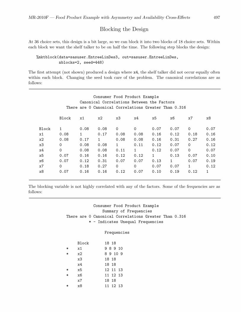
MR-2010F — Food Product Example with Asymmetry and Availability Cross-Effects 497
Blocking the Design
At 36 choice sets, this design is a bit large, so we can block it into two blocks of 18 choice sets. Withineach block we want the shelf talker to be on half the time. The following step blocks the design:
%mktblock(data=sasuser.EntreeLinDes3, out=sasuser.EntreeLinDes,nblocks=2, seed=448)
The first attempt (not shown) produced a design where x4, the shelf talker did not occur equally oftenwithin each block. Changing the seed took care of the problem. The canonical correlations are asfollows:
Consumer Food Product ExampleCanonical Correlations Between the Factors
There are 0 Canonical Correlations Greater Than 0.316
Block x1 x2 x3 x4 x5 x6 x7 x8
Block 1 0.08 0.08 0 0 0.07 0.07 0 0.07x1 0.08 1 0.17 0.08 0.08 0.16 0.12 0.18 0.16x2 0.08 0.17 1 0.08 0.08 0.16 0.31 0.27 0.16x3 0 0.08 0.08 1 0.11 0.12 0.07 0 0.12x4 0 0.08 0.08 0.11 1 0.12 0.07 0 0.07x5 0.07 0.16 0.16 0.12 0.12 1 0.13 0.07 0.10x6 0.07 0.12 0.31 0.07 0.07 0.13 1 0.07 0.19x7 0 0.18 0.27 0 0 0.07 0.07 1 0.12x8 0.07 0.16 0.16 0.12 0.07 0.10 0.19 0.12 1
The blocking variable is not highly correlated with any of the factors. Some of the frequencies are asfollows:
Consumer Food Product ExampleSummary of Frequencies
There are 0 Canonical Correlations Greater Than 0.316* - Indicates Unequal Frequencies
Frequencies
Block 18 18* x1 9 8 9 10* x2 8 9 10 9
x3 18 18x4 18 18
* x5 12 11 13* x6 11 12 13
x7 18 18* x8 11 12 13

498 MR-2010F — Discrete Choice
* Block x1 5 5 4 4 4 4 5 5* Block x2 4 5 4 5 4 4 5 5* Block x3 8 10 9 9
Block x4 9 9 9 9* Block x1 5 4 4 5 4 4 5 5* Block x2 4 4 5 5 4 5 5 4
Block x3 9 9 9 9Block x4 9 9 9 9
* Block x5 6 6 6 6 5 7* Block x6 5 6 7 6 6 6
Block x7 9 9 9 9* Block x8 5 6 7 6 6 6
.
.
.
The blocking variable is perfectly balanced, as it is guaranteed to be if the number of blocks divides thenumber of runs. Balance within blocks, that is the cross-tabulations of the factors with the blockingvariable, looks good. The macro also displays canonical correlations within blocking variables. Thesecan sometimes be quite high, even 1.0, but that is not a problem.∗ The design, as it is displayed bythe %MktBlock macro, is as follows:
Consumer Food Product Example
Block Run x1 x2 x3 x4 x5 x6 x7 x8
1 1 1 3 1 1 1 3 1 12 3 1 2 2 1 3 2 13 2 4 2 2 3 1 1 34 4 3 1 2 2 2 1 15 1 2 2 1 3 3 2 36 4 3 1 1 3 2 2 37 2 3 1 2 1 1 1 38 1 1 2 1 2 2 2 39 4 2 1 2 1 3 2 310 3 1 1 1 1 1 2 311 4 4 2 1 3 2 1 112 4 3 2 2 3 3 1 213 1 4 1 1 2 1 1 214 2 2 1 1 2 3 1 115 1 4 2 2 2 1 2 216 3 4 2 1 1 2 2 217 2 1 1 2 3 2 2 218 3 2 2 2 2 3 1 2
∗Ideally, each subject only makes one choice, since the choice model is based on this assumption (which is almostalways ignored). As the number of blocks increases, the correlations mostly go to one, and ultimately are undefined whenthere is only one choice set per block.
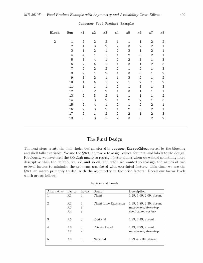
MR-2010F — Food Product Example with Asymmetry and Availability Cross-Effects 499
Consumer Food Product Example
Block Run x1 x2 x3 x4 x5 x6 x7 x8
2 1 4 2 2 1 1 1 2 22 1 3 2 2 3 2 2 13 1 2 1 2 3 1 2 14 4 1 1 1 2 3 2 15 3 4 1 2 2 3 1 36 2 4 1 1 3 1 2 37 2 2 2 2 1 2 1 38 2 1 2 1 3 3 1 29 3 2 1 1 3 2 1 2
10 1 4 1 2 1 2 1 211 1 1 1 2 1 3 1 312 3 2 2 1 3 1 1 113 4 3 2 1 1 1 1 214 3 3 2 1 2 2 1 315 4 4 1 2 1 2 2 116 2 3 2 1 2 3 2 117 4 1 2 2 2 1 2 318 3 3 1 2 3 3 2 2
The Final Design
The next steps create the final choice design, stored in sasuser.EntreeChDes, sorted by the blockingand shelf talker variable. We use the %MktLab macro to assign values, formats, and labels to the design.Previously, we have used the %MktLab macro to reassign factor names when we wanted something moredescriptive than the default, x1, x2, and so on, and when we wanted to reassign the names of twom-level factors to minimize the problems associated with correlated factors. This time, we use the%MktLab macro primarily to deal with the asymmetry in the price factors. Recall our factor levelswhich are as follows:
Factors and Levels
Alternative Factor Levels Brand Description1 X1 4 Client 1.29, 1.69, 2.09, absent
2 X2 4 Client Line Extension 1.39, 1.89, 2.39, absentX3 2 microwave/stove-topX4 2 shelf talker yes/no
3 X5 3 Regional 1.99, 2.49, absent
4 X6 3 Private Label 1.49, 2.29, absentX7 2 microwave/stove-top
5 X8 3 National 1.99 + 2.39, absent

500 MR-2010F — Discrete Choice
The choice design needs a quantitative price attribute, made from all five of the linear price factors,that contains the prices of each of the alternatives. At this point, our factor x1 contains 1, 2, 3, 4, andnot 1.29, 1.69, 2.09, and absent, which is different from x2 and from all of the other factors. A 1 in x1needs to become a price of 1.29 in the choice design, a 1 in x2 needs to become a price of 1.39 in thechoice design, a 1 in x3 needs to become a price of 1.99 in the choice design, and so on. Before we usethe %MktRoll macro to turn the linear arrangement into a choice design, we need to use the %MktLabmacro to assign the actual prices to the price factors.
The %MktLab macro is like the %MktRoll macro in the sense that it can use as input a key= data setthat contains the rules for customizing a design for our particular usage. In the %MktRoll macro, thekey= data set provides the rules for turning a linear arrangement into a choice design. In contrast, inthe %MktLab macro, the key= data set contains the rules for turning a linear arrangement into anotherlinear arrangement, changing one or more of the following: factor names, factor levels, factor types(numeric to character), level formats, and factor labels.
We could use the %MktLab macro to change the names of the variables and their types, but we willnot do that for this example. Ultimately, we use the %MktRoll macro to assign all of the price factorsto a variable called Price and similarly provide meaningful names for all of the factors in the choicedesign, just as we have in previous examples. We could also change a variable like x3 with values of1 and 2 to something like Stove with values ’Stove’ and ’Micro’. We will not do that because wewant to make a design with a simple list of numeric factors, with simple names like x1-x8 that we canrun through the %MktRoll macro to get the final choice design. We assign formats and labels, so wecan display the design in a meaningful way, but ultimately, our only goal at this step is to handle theprice asymmetries by assigning the actual price values to the factors.
The key= data set contains the rules for customizing our design. The data set has as many rows asthe maximum number of levels, in this case four. Each variable is one of the factors in the design, andthe values are the factor levels that we want in the final design. The first factor, x1, is the price factorfor the client brand. Its levels are 1.29, 1.69, and 2.09. In addition, one level is ’not available’, whichis flagged by the SAS special missing value .N. In order to read special missing values in an input dataset, you must use the missing statement and name the expected missing values. The factor x2 has thesame structure as x1, but with different levels. The factor x3 has two levels, hence the key= data sethas missing values in the third and fourth row. Since the design has only 1’s and 2’s for x3, the missingvalues are never used. Notice that we are keeping x3 as a numeric variable with values 1 and 2 usinga format to supply the character levels ’micro’ and ’stove’. The other factors are created in a similarfashion. By default, ordinary missing values ’.’ are not permitted as levels. By default, you can onlyuse ordinary missing values as place holders for factors that have fewer levels than the maximum. Ifyou want missing values in the levels, you must use one of the special missing values .A, .B, ..., .Z,and . ∗ or the cfill= or nfill= options.
The %MktLab macro specification names the input SAS data set with the design and the key data set.By default, it creates an output SAS data set called Final. The data set is sorted by block and shelftalker and displayed in the following steps:
∗Note that the ’.’ in ’.N’ is not typed in the data, nor is it typed in the missing statement. Furthermore, itdoes not appear in the displayed output. However, you need to type it if you ever refer to a special missing value in code:if x1 eq .N then ....

MR-2010F — Food Product Example with Asymmetry and Availability Cross-Effects 501
proc format;value yn 1 = ’No’ 2 = ’Talker’;value micro 1 = ’Micro’ 2 = ’Stove’;run;
data key;missing N;input x1-x8;format x1 x2 x5 x6 x8 dollar5.2
x4 yn. x3 x7 micro.;
label x1 = ’Client Brand’x2 = ’Client Line Extension’x3 = ’Client Micro/Stove’x4 = ’Shelf Talker’
x5 = ’Regional Brand’x6 = ’Private Label’x7 = ’Private Micro/Stove’x8 = ’National Competitor’;
datalines;1.29 1.39 1 1 1.99 1.49 1 1.991.69 1.89 2 2 2.49 2.29 2 2.392.09 2.39 . . N N . NN N . . . . . .;
%mktlab(data=sasuser.EntreeLinDes, key=key)
proc sort out=sasuser.EntreeLinDesLab(drop=run); by block x4; run;
proc print label; id block x4; by block x4; run;
The %MktLab macro displays the variable mapping that it uses, old names followed by new names, asfollows:
Variable Mapping:x1 : x1x2 : x2x3 : x3x4 : x4x5 : x5x6 : x6x7 : x7x8 : x8
In this case, none of the names change, but it is good to make sure that you have the expectedcorrespondence.

502 MR-2010F — Discrete Choice
The design is as follows:
Consumer Food Product Example
Client Client PrivateShelf Client Line Micro/ Regional Private Micro/ National
Block Talker Brand Extension Stove Brand Label Stove Competitor
1 No $1.29 $2.39 Micro $1.99 N Micro $1.99$1.29 $1.89 Stove N N Stove NN $2.39 Micro N $2.29 Stove N
$1.29 $1.39 Stove $2.49 $2.29 Stove N$2.09 $1.39 Micro $1.99 $1.49 Stove NN N Stove N $2.29 Micro $1.99
$1.29 N Micro $2.49 $1.49 Micro $2.39$1.69 $1.89 Micro $2.49 N Micro $1.99$2.09 N Stove $1.99 $2.29 Stove $2.39
1 Talker $2.09 $1.39 Stove $1.99 N Stove $1.99$1.69 N Stove N $1.49 Micro NN $2.39 Micro $2.49 $2.29 Micro $1.99
$1.69 $2.39 Micro $1.99 $1.49 Micro NN $1.89 Micro $1.99 N Stove NN $2.39 Stove N N Micro $2.39
$1.29 N Stove $2.49 $1.49 Stove $2.39$1.69 $1.39 Micro N $2.29 Stove $2.39$2.09 $1.89 Stove $2.49 N Micro $2.39
2 No N $1.89 Stove $1.99 $1.49 Stove $2.39N $1.39 Micro $2.49 N Stove $1.99
$1.69 N Micro N $1.49 Stove N$1.69 $1.39 Stove N N Micro $2.39$2.09 $1.89 Micro N $2.29 Micro $2.39$2.09 $1.89 Stove N $1.49 Micro $1.99N $2.39 Stove $1.99 $1.49 Micro $2.39
$2.09 $2.39 Stove $2.49 $2.29 Micro N$1.69 $2.39 Stove $2.49 N Stove $1.99
2 Talker $1.29 $2.39 Stove N $2.29 Stove $1.99$1.29 $1.89 Micro N $1.49 Stove $1.99$2.09 N Micro $2.49 N Micro N$1.69 $1.89 Stove $1.99 $2.29 Micro N$1.29 N Micro $1.99 $2.29 Micro $2.39$1.29 $1.39 Micro $1.99 N Micro NN N Micro $1.99 $2.29 Stove $1.99N $1.39 Stove $2.49 $1.49 Stove N
$2.09 $2.39 Micro N N Stove $2.39
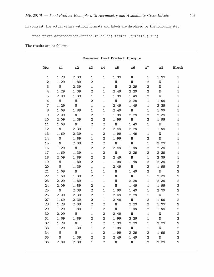
MR-2010F — Food Product Example with Asymmetry and Availability Cross-Effects 503
In contrast, the actual values without formats and labels are displayed by the following step:
proc print data=sasuser.EntreeLinDesLab; format _numeric_; run;
The results are as follows:
Consumer Food Product Example
Obs x1 x2 x3 x4 x5 x6 x7 x8 Block
1 1.29 2.39 1 1 1.99 N 1 1.99 12 1.29 1.89 2 1 N N 2 N 13 N 2.39 1 1 N 2.29 2 N 14 1.29 1.39 2 1 2.49 2.29 2 N 15 2.09 1.39 1 1 1.99 1.49 2 N 16 N N 2 1 N 2.29 1 1.99 17 1.29 N 1 1 2.49 1.49 1 2.39 18 1.69 1.89 1 1 2.49 N 1 1.99 19 2.09 N 2 1 1.99 2.29 2 2.39 1
10 2.09 1.39 2 2 1.99 N 2 1.99 111 1.69 N 2 2 N 1.49 1 N 112 N 2.39 1 2 2.49 2.29 1 1.99 113 1.69 2.39 1 2 1.99 1.49 1 N 114 N 1.89 1 2 1.99 N 2 N 115 N 2.39 2 2 N N 1 2.39 116 1.29 N 2 2 2.49 1.49 2 2.39 117 1.69 1.39 1 2 N 2.29 2 2.39 118 2.09 1.89 2 2 2.49 N 1 2.39 119 N 1.89 2 1 1.99 1.49 2 2.39 220 N 1.39 1 1 2.49 N 2 1.99 221 1.69 N 1 1 N 1.49 2 N 222 1.69 1.39 2 1 N N 1 2.39 223 2.09 1.89 1 1 N 2.29 1 2.39 224 2.09 1.89 2 1 N 1.49 1 1.99 225 N 2.39 2 1 1.99 1.49 1 2.39 226 2.09 2.39 2 1 2.49 2.29 1 N 227 1.69 2.39 2 1 2.49 N 2 1.99 228 1.29 2.39 2 2 N 2.29 2 1.99 229 1.29 1.89 1 2 N 1.49 2 1.99 230 2.09 N 1 2 2.49 N 1 N 231 1.69 1.89 2 2 1.99 2.29 1 N 232 1.29 N 1 2 1.99 2.29 1 2.39 233 1.29 1.39 1 2 1.99 N 1 N 234 N N 1 2 1.99 2.29 2 1.99 235 N 1.39 2 2 2.49 1.49 2 N 236 2.09 2.39 1 2 N N 2 2.39 2

504 MR-2010F — Discrete Choice
One issue remains to be resolved regarding this design, and that concerns the role of the shelf talkerwhen the client line extension is not available. The second part of each block of the design consists ofchoice sets in which the shelf talker is present and calls attention to the client line extension. However,in some of those choice sets, the client line extension is unavailable. This problem can be handled inseveral ways including the following:
• Rerun the design creation and evaluation programs excluding all choice sets with shelf talkerpresent and client line extension unavailable. However, this requires changing the model becausethe excluded cell makes inestimable the interaction between client-line-extension price and shelftalker. Furthermore, the shelf talker variable will almost certainly no longer be balanced.
• Move the choice sets with client line extension unavailable to the no-shelf talker block and reran-domize. The shelf talker is then on for all of the last nine choice sets.
• Let the shelf talker go on and off as needed.
• Let the shelf talker call attention to a brand that happens to be out of stock. It is easy to imaginethis happening in a real store.
Other options are available as well. No one approach is obviously superior to the alternatives. For thisexample, we take the latter approach and let the shelf talker be on even when the client line extensionis not available. Note that if the shelf talker is turned off when the client line extension is not availablethen the design must be manually modified to reflect this fact.
Testing the Design Before Data Collection
This is a complicated design that is used to fit a complicated model with alternative-specific effects,price cross-effects, and availability cross-effects. Collecting data is time consuming and expensive. It isalways good practice, and particularly when there are cross-effects, to make sure that the design workswith the most complicated model that we anticipate fitting. Before we collect any data, we convertthe linear arrangement to a choice design∗ and use the %ChoicEff macro to evaluate its efficiency fora multinomial logit model with both price and availability cross-effects.
For analysis, the design has four factors, Brand, Price, Micro, Shelf. We use the %MktRoll macroand a key= data set (although not the same one as before) to make the choice design. Brand is thealternative name; its values are directly read from the key=Key in-stream data. Price is an attributewhose values are constructed from the factors x1, x2, x5, x6, and x8 in sasuser.EntreeLinDesLabdata set. Micro, the microwave attribute, is constructed from x3 for the client line extension and x7for the private label. Shelf, the shelf talker attribute, is created from x4 for the extension. The keep=option in the %MktRoll macro is used to keep the original price factors in the design, since we needthem for the price cross-effects. Normally, they are dropped. The following steps process the designand display a subset of the results:
∗See page 67 for an explanation of the linear arrangement of a choice design versus the arrangement of a choice designthat is more suitable for analysis.

MR-2010F — Food Product Example with Asymmetry and Availability Cross-Effects 505
data key;input Brand $ 1-10 (Price Micro Shelf) ($);datalines;
Client x1 . .Extension x2 x3 x4Regional x5 . .Private x6 x7 .National x8 . .None . . .;
%mktroll(design=sasuser.EntreeLinDesLab, key=key, alt=brand, out=rolled,keep=x1 x2 x5 x6 x8)
proc print data=sasuser.EntreeLinDesLab(obs=2); run;
proc print data=rolled(obs=12);format price dollar5.2 shelf yn. micro micro.;id set; by set;run;
Consider the first two choice sets in the linear arrangement. They are as follows:
Consumer Food Product Example
Obs x1 x2 x3 x4 x5 x6 x7 x8 Block
1 $1.29 $2.39 Micro No $1.99 N Micro $1.99 12 $1.29 $1.89 Stove No N N Stove N 1
When rolled out as a choice design, they are as follows:
Consumer Food Product Example
Set Brand Price Micro Shelf x1 x2 x5 x6 x8
1 Client $1.29 . . $1.29 $2.39 $1.99 N $1.99Extension $2.39 Micro No $1.29 $2.39 $1.99 N $1.99Regional $1.99 . . $1.29 $2.39 $1.99 N $1.99Private N Micro . $1.29 $2.39 $1.99 N $1.99National $1.99 . . $1.29 $2.39 $1.99 N $1.99None . . . $1.29 $2.39 $1.99 N $1.99

506 MR-2010F — Discrete Choice
2 Client $1.29 . . $1.29 $1.89 N N NExtension $1.89 Stove No $1.29 $1.89 N N NRegional N . . $1.29 $1.89 N N NPrivate N Stove . $1.29 $1.89 N N NNational N . . $1.29 $1.89 N N NNone . . . $1.29 $1.89 N N N
Set 1, Alternative 1
Brand = ’Client’ the brand for this alternativePrice = x1 = $1.29 the price of this alternativeMicro = . does not apply to this brandShelf = . does not apply to this brandx1 = $1.29 the price of the client brand in this choice setx2 = $2.39 the price of the extension in this choice setx5 = $1.99 the price of the regional competitor in this choice setx6 = N the private label unavailable in this choice setx8 = $1.99 national competitor unavailable in this choice set
Set 1, Alternative 2
Brand = ’Extension’ the brand for this alternativePrice = x2 = $2.39 the price of this alternativeMicro = Micro Microwave versionShelf = No Shelf Talker, Nox1 = $1.29 the price of the client brand in this choice setx2 = $2.39 the price of the extension in this choice setx5 = $1.99 the price of the regional competitor in this choice setx6 = N the private label unavailable in this choice setx8 = $1.99 national competitor unavailable in this choice set
The factors x1 through x8 are used to make the price cross-effects. Notice that x1 through x8 areconstant within each choice set. The variable x1 is the price of alternative one, which is the same nomatter which alternative it is stored with. The factors x1 through x8 are also used to make five otherfactors that are used to make the availability cross-effects. The following table shows how the pricesare recoded for those factors:
x1 → a1 x2 → a2 x5 → a5 x6 → a6 x8 → a81.29 1 1.39 1 1.99 1 1.49 1 1.99 11.69 1 1.89 1 2.49 1 2.29 1 2.39 12.09 1 2.39 1 N −2 N −2 N −2
N −3 N −3
This is a contrast coding. Within each factor, the coding sums to zero. Each availability factorhas a coding that contrasts unavailable with the remaining available prices. When an alternative isunavailable, the a variable is set to minus the number of available price points. The coding for availablealternatives is 1. A −3 is used for the first two alternatives that have three prices, and a −2 is usedfor the remaining alternatives that have two prices.

MR-2010F — Food Product Example with Asymmetry and Availability Cross-Effects 507
We need to do a few more things to this design before we are ready to use it. We need to convertthe missings for when Micro and Shelf do not apply to 2 for ’Stove’ and 1 for ’No’. We need to dothe contrast coding for making the availability cross-effects. More is said about this after the code isshown. Since we are treating all of the price factors as a quantitative (not as class variables), we needto convert the missing prices to zero. Eventually, we also need to output just the alternatives that areavailable (those with a nonzero price and also the none alternative). For now, we just make a variablew that flags the available alternatives (w = 1). We can do this using a weight or flag variable: w =1 means available and w = 0 means not available. We also need to assign labels and formats. Thefollowing DATA step does the processing:
data sasuser.EntreeChDes(drop=i);set rolled;array x[6] price x1 -- x8;array a[5] a1 a2 a5 a6 a8;if nmiss(micro) then micro = 2; /* stove if not a factor in alt */if nmiss(shelf) then shelf = 1; /* not talker if not a factor in alt */
a1 = -3 * nmiss(x1) + n(x1); /* alt1: -3 - not avail, 1 - avail */a2 = -3 * nmiss(x2) + n(x2); /* alt2: -3 - not avail, 1 - avail */a5 = -2 * nmiss(x5) + n(x5); /* alt3: -2 - not avail, 1 - avail */a6 = -2 * nmiss(x6) + n(x6); /* alt4: -2 - not avail, 1 - avail */a8 = -2 * nmiss(x8) + n(x8); /* alt5: -2 - not avail, 1 - avail */i = mod(_n_ - 1, 6) + 1; /* alternative number */if i le 5 then a[i] = 0; /* 0 effect of an alt on itself */
do i = 1 to 6; if nmiss(x[i]) then x[i] = 0; end; /* missing price -> 0 */w = brand eq ’None’ or price ne 0; /* 1 - avail, 0 not avail*/format price dollar5.2 shelf yn. micro micro.;label x1 = ’CE, Client’ a1 = ’AE, Client’
x2 = ’CE, Extension’ a2 = ’AE, Extension’x5 = ’CE, Regional’ a5 = ’AE, Regional’x6 = ’CE, Private’ a6 = ’AE, Private’x8 = ’CE, National’ a8 = ’AE, National’;
run;
proc print data=sasuser.EntreeChDes(obs=18); by set; id set; run;
The statements in the middle of the DATA step, from a1 = ... through if i ... create the variablesthat are used to make the availability effects. When alternative 1 is unavailable (x1 is missing), a1 isset to −3, otherwise a1 is set to 1; when alternative 2 is unavailable (x2 is missing), a2 is set to −3,otherwise a2 is set to 1; when alternative 3 is unavailable (x5 is missing), a5 is set to −3, otherwisea5 is set to 1; and so on. Each of these statements could have been written in if else form. Here,for example, is the first assignment statement rewritten: if nmiss(x1) then a1 = −3; else a1 =1;. The variables x1, x2, x5, x6, and x8 are the five price factors, and the “a” factors use thesame numbering scheme, although this is not a requirement. The if i and i = statements then setthe variable to zero when the variable is used to construct the effect of an alternative on itself. Forexample, the first alternative is the client brand, so a1 in the first alternative is set to zero. The firstthree choice sets are as follows:

508 MR-2010F — Discrete Choice
Consumer Food Product Example
Set Brand Price Micro Shelf x1 x2 x5 x6 x8 a1 a2 a5 a6 a8 w
1 Client $1.29 Stove No $1.29 $2.39 $1.99 $0.00 $1.99 0 1 1 -2 1 1Extension $2.39 Micro No $1.29 $2.39 $1.99 $0.00 $1.99 1 0 1 -2 1 1Regional $1.99 Stove No $1.29 $2.39 $1.99 $0.00 $1.99 1 1 0 -2 1 1Private $0.00 Micro No $1.29 $2.39 $1.99 $0.00 $1.99 1 1 1 0 1 0National $1.99 Stove No $1.29 $2.39 $1.99 $0.00 $1.99 1 1 1 -2 0 1None $0.00 Stove No $1.29 $2.39 $1.99 $0.00 $1.99 1 1 1 -2 1 1
2 Client $1.29 Stove No $1.29 $1.89 $0.00 $0.00 $0.00 0 1 -2 -2 -2 1Extension $1.89 Stove No $1.29 $1.89 $0.00 $0.00 $0.00 1 0 -2 -2 -2 1Regional $0.00 Stove No $1.29 $1.89 $0.00 $0.00 $0.00 1 1 0 -2 -2 0Private $0.00 Stove No $1.29 $1.89 $0.00 $0.00 $0.00 1 1 -2 0 -2 0National $0.00 Stove No $1.29 $1.89 $0.00 $0.00 $0.00 1 1 -2 -2 0 0None $0.00 Stove No $1.29 $1.89 $0.00 $0.00 $0.00 1 1 -2 -2 -2 1
3 Client $0.00 Stove No $0.00 $2.39 $0.00 $2.29 $0.00 0 1 -2 1 -2 0Extension $2.39 Micro No $0.00 $2.39 $0.00 $2.29 $0.00 -3 0 -2 1 -2 1Regional $0.00 Stove No $0.00 $2.39 $0.00 $2.29 $0.00 -3 1 0 1 -2 0Private $2.29 Stove No $0.00 $2.39 $0.00 $2.29 $0.00 -3 1 -2 0 -2 1National $0.00 Stove No $0.00 $2.39 $0.00 $2.29 $0.00 -3 1 -2 1 0 0None $0.00 Stove No $0.00 $2.39 $0.00 $2.29 $0.00 -3 1 -2 1 -2 1
In the first choice set, for example, since alternative 1 is available, a1 is 1, for all alternatives exceptthe first, where a1 is 0. Also in the first choice set, since alternative 4 is not available and there aretwo price levels, a6 is −2 for all alternatives except the fourth, where a6 is 0. In the third choice set,since alternative 1 is not available and there are three price levels, a1 is −3, for all alternatives exceptthe first, where a2 is 0. In general, the coding stores a zero in the ith effect for the ith alternative,otherwise a 1 if the alternative is available, otherwise minus the number of price levels if the alternativeis unavailable.
Now our choice design is done except for the final coding for the analysis. We can now use the%ChoicEff macro to evaluate our choice design. The complicated part of this is the model due to thealternative-specific price effects and the cross-effects. For now, let’s concentrate on everything else.The following step provides some sample code, omitting for now the details of the model (indicated bymodel= ...):
%choiceff(data=sasuser.EntreeChDes, /* candidate set of choice sets */init=sasuser.EntreeChDes(keep=set), /* select these sets */intiter=0, /* evaluate without internal iterations */model= ..., /* model specification skipped for now */nsets=36, /* number of choice sets */nalts=6, /* number of alternatives */weight=w, /* weight to handle unavailable alts */beta=zero) /* assumed beta vector, Ho: b=0 */

MR-2010F — Food Product Example with Asymmetry and Availability Cross-Effects 509
The way you check the efficiency of a design like this is to first name it in the data= option. This is thecandidate set that contains all of the choice sets that we will consider. In addition, the same designis named in the init= option. The full specification is init=sasuser.EntreeChDes(keep=set). Justthe variable Set is kept. It is used to bring in just the indicated choice sets from the data= design,which in this case is all of them. The option nsets=36 specifies the number of choice sets, and nalts=6specifies the number of alternatives. This macro requires a constant number of alternatives in eachchoice set for ease of data management. However, not all of the alternatives have to be used. In thiscase, we have an availability study. We need to keep the unavailable alternatives in the design forthis step, but we do not want them to contribute to the analysis, so we specify a weight variable withweight=w and flag the available alternatives with w=1 and the unavailable alternatives with w=0. Theoption beta=zero specifies that we are assuming for design evaluation purpose all zero betas. We canspecify other values and get other results for the variances and standard errors. Finally, we specifyintiter=0 which specifies zero internal iterations. We use zero internal iterations when we want toevaluate an initial design, but not attempt to improve it. The actual specification we use, completewith the model specification, is shown in the following step:
%choiceff(data=sasuser.EntreeChDes, /* candidate set of choice sets */init=sasuser.EntreeChDes(keep=set), /* select these sets */intiter=0, /* evaluate without internal iterations */
/* cross-effects model *//* zero=’None’ - ’None’ level is ref lev*/
model=class(brand / zero=’None’)/* use blank sep to build interact terms*/
class(brand / zero=’None’ separators=’’ ’ ’) *identity(price)
/* lpr=5 0 uses 5 var name chars in *//* label for shelf and 0 for micro *//* ’No’ is ref level for shelf *//* ’Stove’ is ref level for micro */
class(shelf micro / lprefix=5 0 zero=’No’ ’Stove’)/* ’ on ’ is used to build interact term*/
identity(x1 x2 x5 x6 x8) *class(brand / zero=’None’ separators=’ ’ ’ on ’)
identity(a1 a2 a5 a6 a8) *class(brand / zero=’None’ separators=’ ’ ’ on ’) /
lprefix=0 /* lpr=0 labels are created from just *//* levels unless overridden above */
order=data, /* order=data - do not sort levels */
nsets=36, /* number of choice sets */nalts=6, /* number of alternatives */weight=w, /* weight to handle unavailable alts */beta=zero) /* assumed beta vector, Ho: b=0 */
The specification class(brand / zero=’None’) specifies the brand effects. This specification cre-ates indicator variables for brand with the constant alternative being the reference brand. The op-tion zero=’None’ ensures that the reference level is ’None’ instead of the default last sorted level(’Regional’). Indicator variables are created for the brands Client, Extension, Regional, Private, andNational, but not None. The zero=’None’ option, like zero=’Home’ and other zero=’literal-string’

510 MR-2010F — Discrete Choice
options we have used in previous examples, names the actual formatted value of the class variable thatshould be excluded from the coded variables because the coefficient is zero. Do not confuse zero=noneand zero=’None’. The zero=none option specifies that you want all indicator variables to be cre-ated, even including one for the last level. In contrast, the option zero=’None’ (or zero= any quotedstring) names a specific formatted value, in this case ’None’, for which indicator variables are not tobe created. See page 78 for more information about the zero= option.
The specification class(brand / ...) * identity(price) creates the alternative-specific price ef-fects. They are specified as an interaction between a categorical variable Brand and a quantitativeattribute Price. The separators=’’ ’ ’ option in the class specification specifies the separatorsthat are used to construct the labels for the main effect and interaction terms. The main-effects separa-tor, which is the first separators= value, ’’, is ignored since lprefix=0. Specifying ’ ’ as the secondvalue creates labels of the form brand-blank-price instead of the default brand-blank-asterisk-blank-price.
The specification class(shelf micro / ...) names the shelf talker and microwave variables ascategorical variables and creates indicator variables for the ’Talker’ category, not the ’No’ categoryand the ’Micro’ category not the ’Stove’ category. In zero=’No’ ’Stove’, the ’No’ applies to thefirst variable, Shelf and the second value, ’Stove’, applies to second variable, Micro.
The specification identity(x1 x2 x5 x6 x8) * class(brand / ...) creates the linear price cross-effects. The separators= option is specified with a second value of ’ on ’ to create cross-effectlabels like ’Client on Extension’. The specification identity(a1 a2 a5 a6 a8) * class(brand/ ...) creates the availability cross-effects. Note that the order of the transformation specification isimportant. Make sure you specify identity followed by class in order to get the right labels. Moreis said about cross-effects when we look at the actual coded values in the next few pages.
PROC TRANSREG produces the following warning:
WARNING: This usage of * sets one group’s slope to zero. Specify |to allow all slopes and intercepts to vary. Alternatively,specify CLASS(vars) * identity(vars) identity(vars) forseparate within group functions and a common intercept.This is a change from Version 6.
This is because class is interacted with identity using the asterisk instead of the vertical bar. In alinear model, this might be a sign of a coding error, so the procedure displays a warning. If you getthis warning while coding a choice model specifying zero=’constant-alternative-level’, you can safelyignore it. Still, it is always good to display one or more coded choice sets to check the coding as wewill do later. The last part of the output from the %ChoicEff macro is as follows:
Consumer Food Product Example
Final Results
Design 1Choice Sets 36Alternatives 6Parameters 52Maximum Parameters 180D-Efficiency 0D-Error .

MR-2010F — Food Product Example with Asymmetry and Availability Cross-Effects 511
Consumer Food Product Example
Standardn Variable Name Label Variance DF Error
1 BrandClient Client 69.807 1 8.35512 BrandExtension Extension 75.688 1 8.69993 BrandRegional Regional 121.147 1 11.00674 BrandPrivate Private 104.058 1 10.20095 BrandNational National 110.456 1 10.50986 BrandClientPrice Client Price 3.255 1 1.80427 BrandExtensionPrice Extension Price 2.233 1 1.49428 BrandRegionalPrice Regional Price 6.599 1 2.56889 BrandPrivatePrice Private Price 2.604 1 1.613810 BrandNationalPrice National Price 11.071 1 3.327311 ShelfTalker Shelf Talker 0.928 1 0.9636
12 MicroMicro Micro 0.562 1 0.749313 x1BrandClient CE, Client on Client . 0 .14 x1BrandExtension CE, Client on Extension 4.689 1 2.165515 x1BrandRegional CE, Client on Regional 4.462 1 2.112416 x1BrandPrivate CE, Client on Private 5.627 1 2.372017 x1BrandNational CE, Client on National 5.374 1 2.3182
18 x2BrandClient CE, Extension on Client 3.040 1 1.743519 x2BrandExtension CE, Extension on Extension . 0 .20 x2BrandRegional CE, Extension on Regional 3.038 1 1.743121 x2BrandPrivate CE, Extension on Private 3.666 1 1.914622 x2BrandNational CE, Extension on National 3.130 1 1.7691
23 x5BrandClient CE, Regional on Client 8.961 1 2.993524 x5BrandExtension CE, Regional on Extension 9.824 1 3.134325 x5BrandRegional CE, Regional on Regional . 0 .26 x5BrandPrivate CE, Regional on Private 10.496 1 3.239827 x5BrandNational CE, Regional on National 10.360 1 3.2188
28 x6BrandClient CE, Private on Client 3.965 1 1.991229 x6BrandExtension CE, Private on Extension 4.195 1 2.048230 x6BrandRegional CE, Private on Regional 4.429 1 2.104631 x6BrandPrivate CE, Private on Private . 0 .32 x6BrandNational CE, Private on National 4.453 1 2.1102
33 x8BrandClient CE, National on Client 18.098 1 4.254134 x8BrandExtension CE, National on Extension 16.311 1 4.038735 x8BrandRegional CE, National on Regional 22.372 1 4.729936 x8BrandPrivate CE, National on Private 18.271 1 4.274537 x8BrandNational CE, National on National . 0 .
38 a1BrandClient AE, Client on Client . 0 .39 a1BrandExtension AE, Client on Extension 0.981 1 0.990440 a1BrandRegional AE, Client on Regional 0.892 1 0.944741 a1BrandPrivate AE, Client on Private 1.071 1 1.034742 a1BrandNational AE, Client on National 1.031 1 1.0155

512 MR-2010F — Discrete Choice
43 a2BrandClient AE, Extension on Client 0.766 1 0.875544 a2BrandExtension AE, Extension on Extension . 0 .45 a2BrandRegional AE, Extension on Regional 0.880 1 0.938146 a2BrandPrivate AE, Extension on Private 0.990 1 0.995247 a2BrandNational AE, Extension on National 0.999 1 0.9995
48 a5BrandClient AE, Regional on Client 5.128 1 2.264449 a5BrandExtension AE, Regional on Extension 5.530 1 2.351650 a5BrandRegional AE, Regional on Regional . 0 .51 a5BrandPrivate AE, Regional on Private 5.860 1 2.420852 a5BrandNational AE, Regional on National 5.887 1 2.4263
53 a6BrandClient AE, Private on Client 1.796 1 1.340254 a6BrandExtension AE, Private on Extension 1.843 1 1.357755 a6BrandRegional AE, Private on Regional 2.116 1 1.454756 a6BrandPrivate AE, Private on Private . 0 .57 a6BrandNational AE, Private on National 1.964 1 1.4015
58 a8BrandClient AE, National on Client 10.135 1 3.183659 a8BrandExtension AE, National on Extension 8.720 1 2.952960 a8BrandRegional AE, National on Regional 12.021 1 3.467161 a8BrandPrivate AE, National on Private 10.188 1 3.191962 a8BrandNational AE, National on National . 0 .
==52
First we see estimable brand effects for each of the five brands, excluding the constant alternative’None’. Next, we see quantitative alternative-specific price effects for each of the brands. The nexttwo effects that are single df effects for the shelf talker and the microwave option. Then we see five setsof linear price cross-effects (those whose label begins with “CE”), each consisting of four effects of abrand on another brand, plus one more zero df cross-effect of a brand on itself. The zero df and missingvariances and standard errors are correct since the cross-effect of an alternative on itself is perfectlyaliased with its alternative-specific price effect. After that we see five sets of availability cross-effects(those whose label begins with “AE”), each consisting of four effects of a brand on another brand, plusone more zero df cross-effect of a brand on itself. The zero df and missing variances and standard errorsare correct since the cross-effect of an alternative on itself is zero. These results look fine. Everythingthat should be estimable is estimable, and everything that should not be estimable is not.
Next, we run some further checks by looking at the coded design. Before we look at the coded design,recall that the design for the first five choice sets is as follows:

MR-2010F — Food Product Example with Asymmetry and Availability Cross-Effects 513
Consumer Food Product Example
Client Client PrivateShelf Client Line Micro/ Regional Private Micro/ National
Block Talker Brand Extension Stove Brand Label Stove Competitor
1 No $1.29 $2.39 Micro $1.99 N Micro $1.99$1.29 $1.89 Stove N N Stove N
N $2.39 Micro N $2.29 Stove N$1.29 $1.39 Stove $2.49 $2.29 Stove N$2.09 $1.39 Micro $1.99 $1.49 Stove N
The coded design that the %ChoicEff macro creates is called TMP CAND. We can look at the codeddata set in several ways. First, the Brand, Price, microwave and shelf talker factors, for just theavailable alternatives for the first five choice sets are displayed as follows:
proc print data=tmp_cand(obs=24) label;var Brand Price Shelf Micro;where w;run;
The results are as follows:
Consumer Food Product Example
Obs Brand Price Shelf Micro
1 Client $1.29 No Stove2 Extension $2.39 No Micro3 Regional $1.99 No Stove5 National $1.99 No Stove6 None $0.00 No Stove
7 Client $1.29 No Stove8 Extension $1.89 No Stove12 None $0.00 No Stove14 Extension $2.39 No Micro16 Private $2.29 No Stove18 None $0.00 No Stove
19 Client $1.29 No Stove20 Extension $1.39 No Stove21 Regional $2.49 No Stove22 Private $2.29 No Stove24 None $0.00 No Stove

514 MR-2010F — Discrete Choice
25 Client $2.09 No Stove26 Extension $1.39 No Micro27 Regional $1.99 No Stove28 Private $1.49 No Stove30 None $0.00 No Stove
34 Private $2.29 No Micro35 National $1.99 No Stove36 None $0.00 No Stove
Unlike all previous examples, the number of alternatives is not the same in all of the choice sets dueto differing subsets of brands being unavailable in each choice set.
The coded factors for the brand effects and alternative-specific price effects for the first choice set aredisplayed as follows:
proc print data=tmp_cand(obs=5) label;id Brand;var BrandClient -- BrandNational;where w;run;
proc format; value zer 0 = ’ 0’; run;
proc print data=tmp_cand(obs=5) label;id Brand Price;var BrandClientPrice -- BrandNationalPrice;format BrandClientPrice -- BrandNationalPrice zer5.2;where w;run;
The results are as follows:
Consumer Food Product Example
Brand Client Extension Regional Private National
Client 1 0 0 0 0Extension 0 1 0 0 0Regional 0 0 1 0 0National 0 0 0 0 1None 0 0 0 0 0

MR-2010F — Food Product Example with Asymmetry and Availability Cross-Effects 515
Consumer Food Product Example
Client Extension Regional Private NationalBrand Price Price Price Price Price Price
Client $1.29 1.29 0 0 0 0Extension $2.39 0 2.39 0 0 0Regional $1.99 0 0 1.99 0 0National $1.99 0 0 0 0 1.99None $0.00 0 0 0 0 0
The brand effects and alternative-specific price effect codings are similar to those we have used previ-ously. The difference is the presence of all zero columns for unavailable alternatives, in this case theprivate label and national brands. Note that Brand Price are just ID variables and do not enter intothe analysis.
The shelf talker and microwave coded factors (along with the Brand, Price, Shelf, and Micro factors)are displayed by the following step:
proc print data=tmp_cand(obs=5) label;id Brand Price Shelf Micro;var shelftalker micromicro;where w;run;
The results are as follows:
Consumer Food Product Example
ShelfBrand Price Shelf Micro Talker Micro
Client $1.29 No Stove 0 0Extension $2.39 No Micro 0 1Regional $1.99 No Stove 0 0National $1.99 No Stove 0 0None $0.00 No Stove 0 0
The following steps display the price cross-effects along with Brand and Price for the first choice set:
proc print data=tmp_cand(obs=4) label;id Brand Price;var x1Brand:; format x1Brand: zer5.2;where w;run;

516 MR-2010F — Discrete Choice
proc print data=tmp_cand(obs=4) label;id Brand Price;var x2Brand:; format x2Brand: zer5.2;where w;run;
proc print data=tmp_cand(obs=4) label;id Brand Price;var x5Brand:; format x5Brand: zer5.2;where w;run;
proc print data=tmp_cand(obs=4) label;id Brand Price;var x6Brand:; format x6Brand: zer5.2;where w;run;
proc print data=tmp_cand(obs=4) label;id Brand Price;var x8Brand:; format x8Brand: zer5.2;where w;run;
The cross-effects are displayed in panels. This first panel shows the terms that capture the effect ofthe client brand on the utility of the other brands. The second panel shows the terms that capture theeffect of the line extension on the other alternatives, and so on. An unavailable brand has no effect onany other brand’s utility in that choice set. The results are as follows:
Consumer Food Product Example
CE, Client CE, Client CE, ClientCE, Client on on CE, Client on
Brand Price on Client Extension Regional on Private National
Client $1.29 1.29 0 0 0 0Extension $2.39 0 1.29 0 0 0Regional $1.99 0 0 1.29 0 0National $1.99 0 0 0 0 1.29
CE, CE, CE,CE, Extension Extension CE, Extension
Extension on on Extension onBrand Price on Client Extension Regional on Private National
Client $1.29 2.39 0 0 0 0Extension $2.39 0 2.39 0 0 0Regional $1.99 0 0 2.39 0 0National $1.99 0 0 0 0 2.39

MR-2010F — Food Product Example with Asymmetry and Availability Cross-Effects 517
CE, CE, CE,CE, Regional Regional CE, Regional
Regional on on Regional onBrand Price on Client Extension Regional on Private National
Client $1.29 1.99 0 0 0 0Extension $2.39 0 1.99 0 0 0Regional $1.99 0 0 1.99 0 0National $1.99 0 0 0 0 1.99
CE, CE, CE, CE, CE,Private on Private on Private on Private on Private on
Brand Price Client Extension Regional Private National
Client $1.29 0 0 0 0 0Extension $2.39 0 0 0 0 0Regional $1.99 0 0 0 0 0National $1.99 0 0 0 0 0
CE, CE, CE,CE, National National CE, National
National on on National onBrand Price on Client Extension Regional on Private National
Client $1.29 1.99 0 0 0 0Extension $2.39 0 1.99 0 0 0Regional $1.99 0 0 1.99 0 0National $1.99 0 0 0 0 1.99
A column like ’CE, Client on Extension’ in the first panel, for example, captures the effect of theclient brand at $1.29 on the utility of the extension. In the next panel, ’CE, Extension on Client’captures the effect of the extension at $2.39 on the utility of the client brand.
The following steps displays the availability cross-effects along with Brand and Price for the first choiceset:
proc print data=tmp_cand(obs=4) label;id Brand Price;var a1Brand:;where w;run;
proc print data=tmp_cand(obs=4) label;id Brand Price;var a2Brand:;where w;run;
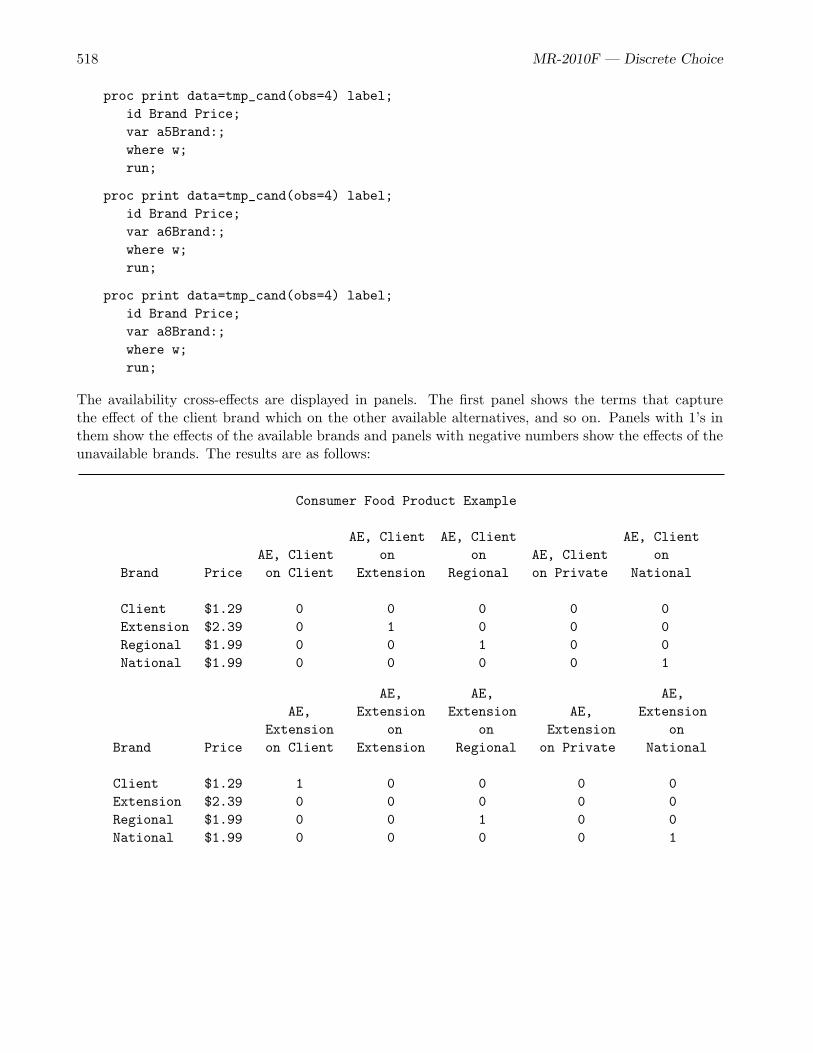
518 MR-2010F — Discrete Choice
proc print data=tmp_cand(obs=4) label;id Brand Price;var a5Brand:;where w;run;
proc print data=tmp_cand(obs=4) label;id Brand Price;var a6Brand:;where w;run;
proc print data=tmp_cand(obs=4) label;id Brand Price;var a8Brand:;where w;run;
The availability cross-effects are displayed in panels. The first panel shows the terms that capturethe effect of the client brand which on the other available alternatives, and so on. Panels with 1’s inthem show the effects of the available brands and panels with negative numbers show the effects of theunavailable brands. The results are as follows:
Consumer Food Product Example
AE, Client AE, Client AE, ClientAE, Client on on AE, Client on
Brand Price on Client Extension Regional on Private National
Client $1.29 0 0 0 0 0Extension $2.39 0 1 0 0 0Regional $1.99 0 0 1 0 0National $1.99 0 0 0 0 1
AE, AE, AE,AE, Extension Extension AE, Extension
Extension on on Extension onBrand Price on Client Extension Regional on Private National
Client $1.29 1 0 0 0 0Extension $2.39 0 0 0 0 0Regional $1.99 0 0 1 0 0National $1.99 0 0 0 0 1
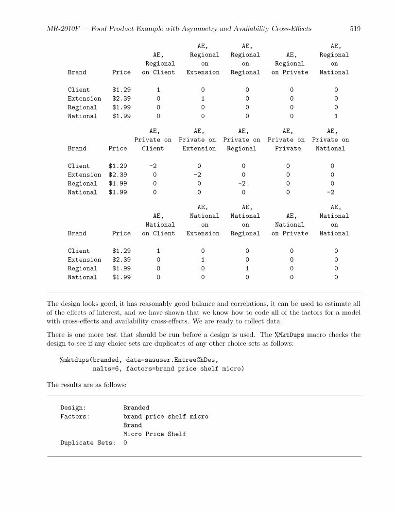
MR-2010F — Food Product Example with Asymmetry and Availability Cross-Effects 519
AE, AE, AE,AE, Regional Regional AE, Regional
Regional on on Regional onBrand Price on Client Extension Regional on Private National
Client $1.29 1 0 0 0 0Extension $2.39 0 1 0 0 0Regional $1.99 0 0 0 0 0National $1.99 0 0 0 0 1
AE, AE, AE, AE, AE,Private on Private on Private on Private on Private on
Brand Price Client Extension Regional Private National
Client $1.29 -2 0 0 0 0Extension $2.39 0 -2 0 0 0Regional $1.99 0 0 -2 0 0National $1.99 0 0 0 0 -2
AE, AE, AE,AE, National National AE, National
National on on National onBrand Price on Client Extension Regional on Private National
Client $1.29 1 0 0 0 0Extension $2.39 0 1 0 0 0Regional $1.99 0 0 1 0 0National $1.99 0 0 0 0 0
The design looks good, it has reasonably good balance and correlations, it can be used to estimate allof the effects of interest, and we have shown that we know how to code all of the factors for a modelwith cross-effects and availability cross-effects. We are ready to collect data.
There is one more test that should be run before a design is used. The %MktDups macro checks thedesign to see if any choice sets are duplicates of any other choice sets as follows:
%mktdups(branded, data=sasuser.EntreeChDes,nalts=6, factors=brand price shelf micro)
The results are as follows:
Design: BrandedFactors: brand price shelf micro
BrandMicro Price Shelf
Duplicate Sets: 0

520 MR-2010F — Discrete Choice
The first line of the table tells us that this is a branded design as opposed to a generic design (bundlesof attributes with no brands). The second line tells us the factors as specified in the factors= option.These are followed by the actual variable names for the factors. The last line reports the number ofduplicates. In this case, there are no duplicate choice sets. If there are duplicate choice sets, thenchanging the random number seed might help. Changing other aspects of the design or the approachfor making the design might help as well.
Generating Artificial Data
We do not illustrate questionnaire generation for this example since we have done it several times beforein previous examples. Instead we go straight to data processing and analysis. The following DATAstep generates some artificial data:†
%let m = 6;%let mm1 = %eval(&m - 1);%let n = 36;
proc format;value yn 1 = ’No’ 2 = ’Talker’;value micro 1 = ’Micro’ 2 = ’Stove’;run;
†This section shows in a cursory way how to generate artificial data. Some researchers wisely like to use artificial datato test a design before spending lots of money on collecting data. See the section beginning on page 393 for a detaileddiscussion of generating artificial data.

MR-2010F — Food Product Example with Asymmetry and Availability Cross-Effects 521
data _null_;array brands[&m] _temporary_ (5 7 1 2 3 -2);array u[&m];array x[&mm1] x1 x2 x5 x6 x8;do rep = 1 to 300;
if mod(rep, 2) then put;put rep 3. +2 @@;do j = 1 to &n;
set sasuser.EntreeLinDesLab point=j;do brand = 1 to &m; u[brand] = brands[brand] + 2 * normal(17); end;do brand = 1 to &mm1;
if n(x[brand]) then u[brand] + -x[brand]; else u[brand] = .;end;
if n(u2) and x4 = 2 then u2 + 1; /* shelf talker */if n(u2) and x3 = 1 then u2 + 1; /* microwave */if n(u4) and x7 = 1 then u4 + 1; /* microwave */* Choose the most preferred alternative.;m = max(of u1-u&m);do brand = 1 to &m;
if n(u[brand]) then if abs(u[brand] - m) < 1e-4 then c = brand;end;
put +(-1) c @@;end;
end;stop;run;
Creating artificial data and trying the analysis before collecting real data is another way to test thedesign before going to the expense of data collection. The following DATA step reads the data:
data results;input Subj (choose1-choose&n) (1.) @@;datalines;
1 222224155212222522221221222221212522 2 2222254212422221222212122222212113223 212224521545222122221222221121112522 4 2121251212122221222212224212212125225 222225125212222122521212222221212422 6 222125523112222122224221212111242522...
297 222225521212222422224222522121151622 298 222224121242122422221222512221212522299 112225121212122121521222212211212622 300 122225123242122122221211222123212322;
Processing the Data
The analysis proceeds in a fashion similar to before. We have already made the choice design, so wejust have to merge it with the data. The data and design are merged in the usual way using the%MktMerge macro. Notice at this point that the unavailable alternatives are still in the design. The
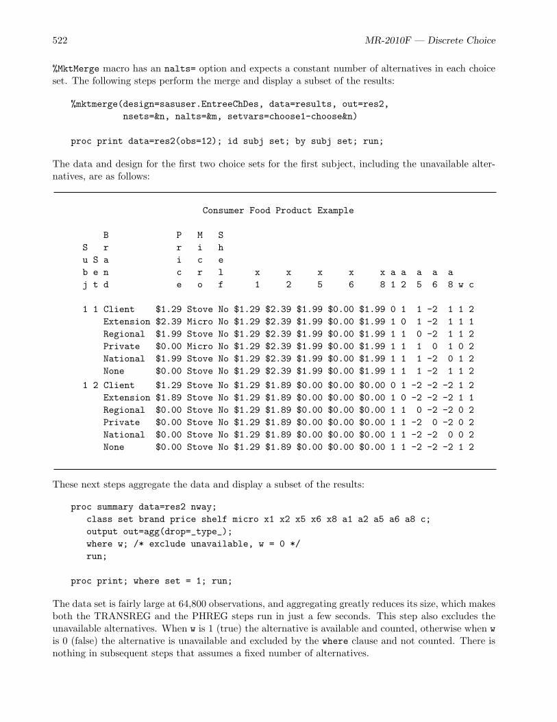
522 MR-2010F — Discrete Choice
%MktMerge macro has an nalts= option and expects a constant number of alternatives in each choiceset. The following steps perform the merge and display a subset of the results:
%mktmerge(design=sasuser.EntreeChDes, data=results, out=res2,nsets=&n, nalts=&m, setvars=choose1-choose&n)
proc print data=res2(obs=12); id subj set; by subj set; run;
The data and design for the first two choice sets for the first subject, including the unavailable alter-natives, are as follows:
Consumer Food Product Example
B P M SS r r i hu S a i c eb e n c r l x x x x x a a a a aj t d e o f 1 2 5 6 8 1 2 5 6 8 w c
1 1 Client $1.29 Stove No $1.29 $2.39 $1.99 $0.00 $1.99 0 1 1 -2 1 1 2Extension $2.39 Micro No $1.29 $2.39 $1.99 $0.00 $1.99 1 0 1 -2 1 1 1Regional $1.99 Stove No $1.29 $2.39 $1.99 $0.00 $1.99 1 1 0 -2 1 1 2Private $0.00 Micro No $1.29 $2.39 $1.99 $0.00 $1.99 1 1 1 0 1 0 2National $1.99 Stove No $1.29 $2.39 $1.99 $0.00 $1.99 1 1 1 -2 0 1 2None $0.00 Stove No $1.29 $2.39 $1.99 $0.00 $1.99 1 1 1 -2 1 1 2
1 2 Client $1.29 Stove No $1.29 $1.89 $0.00 $0.00 $0.00 0 1 -2 -2 -2 1 2Extension $1.89 Stove No $1.29 $1.89 $0.00 $0.00 $0.00 1 0 -2 -2 -2 1 1Regional $0.00 Stove No $1.29 $1.89 $0.00 $0.00 $0.00 1 1 0 -2 -2 0 2Private $0.00 Stove No $1.29 $1.89 $0.00 $0.00 $0.00 1 1 -2 0 -2 0 2National $0.00 Stove No $1.29 $1.89 $0.00 $0.00 $0.00 1 1 -2 -2 0 0 2None $0.00 Stove No $1.29 $1.89 $0.00 $0.00 $0.00 1 1 -2 -2 -2 1 2
These next steps aggregate the data and display a subset of the results:
proc summary data=res2 nway;class set brand price shelf micro x1 x2 x5 x6 x8 a1 a2 a5 a6 a8 c;output out=agg(drop=_type_);where w; /* exclude unavailable, w = 0 */run;
proc print; where set = 1; run;
The data set is fairly large at 64,800 observations, and aggregating greatly reduces its size, which makesboth the TRANSREG and the PHREG steps run in just a few seconds. This step also excludes theunavailable alternatives. When w is 1 (true) the alternative is available and counted, otherwise when wis 0 (false) the alternative is unavailable and excluded by the where clause and not counted. There isnothing in subsequent steps that assumes a fixed number of alternatives.

MR-2010F — Food Product Example with Asymmetry and Availability Cross-Effects 523
All of the variables used in the analysis are named as class variables in PROC SUMMARY, whichreduces the data set from 64,800 observations to 286. The aggregated data for the first choice set is asfollows:
Consumer Food Product Example
_B P S M Fr r h i R
O S a i e c Eb e n c l r x x x x x a a a a a Qs t d e f o 1 2 5 6 8 1 2 5 6 8 c _
1 1 Client $1.29 No Stove $1.29 $2.39 $1.99 $0.00 $1.99 0 1 1 -2 1 1 742 1 Client $1.29 No Stove $1.29 $2.39 $1.99 $0.00 $1.99 0 1 1 -2 1 2 2263 1 Extension $2.39 No Micro $1.29 $2.39 $1.99 $0.00 $1.99 1 0 1 -2 1 1 2204 1 Extension $2.39 No Micro $1.29 $2.39 $1.99 $0.00 $1.99 1 0 1 -2 1 2 805 1 National $1.99 No Stove $1.29 $2.39 $1.99 $0.00 $1.99 1 1 1 -2 0 1 66 1 National $1.99 No Stove $1.29 $2.39 $1.99 $0.00 $1.99 1 1 1 -2 0 2 2947 1 None $0.00 No Stove $1.29 $2.39 $1.99 $0.00 $1.99 1 1 1 -2 1 2 3008 1 Regional $1.99 No Stove $1.29 $2.39 $1.99 $0.00 $1.99 1 1 0 -2 1 2 300
In the first choice set, the client brand is chosen (c = 1) a total of freq = 74 times and not chosen(c = 2) a total of freq = 226 times. Each alternative is chosen and not chosen a total of 300 times,which is the number of subjects. These next steps code and run the analysis.
Cross-Effects
This next step codes the design for analysis. This coding is discussed on page 509. PROC TRANSREGis run like before, except now the data set Agg is specified and the ID variable includes freq (thefrequency variable) but not Subj (the subject number variable). The following step does the coding:
proc transreg data=agg design=5000 nozeroconstant norestoremissing;model class(brand / zero=’None’)
class(brand / zero=’None’ separators=’’ ’ ’) * identity(price)class(shelf micro / lprefix=5 0 zero=’No’ ’Stove’)identity(x1 x2 x5 x6 x8) *
class(brand / zero=’None’ separators=’ ’ ’ on ’)identity(a1 a2 a5 a6 a8) *
class(brand / zero=’None’ separators=’ ’ ’ on ’) /lprefix=0;
output out=coded(drop=_type_ _name_ intercept);id set c _freq_;label shelf = ’Shelf Talker’
micro = ’Microwave’;run;

524 MR-2010F — Discrete Choice
Note that like we saw in the %ChoicEff macro, PROC TRANSREG produces the following warning:
WARNING: This usage of * sets one group’s slope to zero. Specify |to allow all slopes and intercepts to vary. Alternatively,specify CLASS(vars) * identity(vars) identity(vars) forseparate within group functions and a common intercept.This is a change from Version 6.
This is because class is interacted with identity using the asterisk instead of the vertical bar. In alinear model, this might be a sign of a coding error, so the procedure displays a warning. If you getthis warning while coding a choice model specifying zero=’constant-alternative-level’, you can safelyignore it.
The analysis is the same as we have done previously with aggregate data. PROC PHREG is run to fitthe mother logit model, complete with availability cross-effects as follows:
proc phreg data=coded;strata set;model c*c(2) = &_trgind / ties=breslow;freq _freq_;run;
Multinomial Logit Model Results
Recall that we used %phchoice(on) on page 287 to customize the output from PROC PHREG. Thesesteps produced the following results:
Consumer Food Product Example
The PHREG Procedure
Model Information
Data Set WORK.CODEDDependent Variable cCensoring Variable cCensoring Value(s) 2Frequency Variable _FREQ_Ties Handling BRESLOW
Number of Observations Read 284Number of Observations Used 284Sum of Frequencies Read 47400Sum of Frequencies Used 47400

MR-2010F — Food Product Example with Asymmetry and Availability Cross-Effects 525
Summary of Subjects, Sets, and Chosen and Unchosen Alternatives
Number of Chosen NotStratum Set Alternatives Alternatives Chosen
1 1 1500 300 12002 2 900 300 6003 3 900 300 6004 4 1500 300 12005 5 1500 300 12006 6 900 300 6007 7 1500 300 12008 8 1500 300 12009 9 1500 300 120010 10 1500 300 120011 11 900 300 60012 12 1500 300 120013 13 1500 300 120014 14 900 300 60015 15 900 300 60016 16 1500 300 120017 17 1500 300 120018 18 1500 300 120019 19 1500 300 120020 20 1200 300 90021 21 900 300 60022 22 1200 300 90023 23 1500 300 120024 24 1500 300 120025 25 1500 300 120026 26 1500 300 120027 27 1500 300 120028 28 1500 300 120029 29 1500 300 120030 30 900 300 60031 31 1500 300 120032 32 1500 300 120033 33 1200 300 90034 34 1200 300 90035 35 1200 300 90036 36 1200 300 900
---------------------------------------------------------------Total 47400 10800 36600
Convergence Status
Convergence criterion (GCONV=1E-8) satisfied.

526 MR-2010F — Discrete Choice
Model Fit Statistics
Without WithCriterion Covariates Covariates
-2 LOG L 154710.28 134305.63AIC 154710.28 134409.63SBC 154710.28 134788.57
Testing Global Null Hypothesis: BETA=0
Test Chi-Square DF Pr > ChiSq
Likelihood Ratio 20404.6461 52 <.0001Score 22883.7078 52 <.0001Wald 6444.0844 52 <.0001
Multinomial Logit Parameter Estimates
Parameter StandardDF Estimate Error Chi-Square Pr > ChiSq
Client 1 8.16629 3.96395 4.2442 0.0394Extension 1 10.30298 4.13379 6.2119 0.0127National 1 5.41386 4.90468 1.2184 0.2697Private 1 4.90773 4.06749 1.4558 0.2276Regional 1 4.96459 5.93423 0.6999 0.4028
Client Price 1 -1.11653 0.77149 2.0945 0.1478Extension Price 1 -0.99948 1.21987 0.6713 0.4126National Price 1 1.25938 1.74132 0.5231 0.4695Private Price 1 -1.33471 0.76283 3.0614 0.0802Regional Price 1 -1.22852 1.48246 0.6867 0.4073
Shelf Talker 1 0.66941 0.07828 73.1204 <.0001
Micro 1 0.59645 0.06746 78.1706 <.0001CE, Client on Client 0 0 . . .CE, Client on Extension 1 -0.31640 0.78240 0.1635 0.6859CE, Client on National 1 -0.50555 0.80031 0.3990 0.5276CE, Client on Private 1 -0.25802 0.82061 0.0989 0.7532CE, Client on Regional 1 1.15121 1.03011 1.2489 0.2638
CE, Extension on Client 1 -0.52993 1.22364 0.1876 0.6650CE, Extension on Extension 0 0 . . .CE, Extension on National 1 -0.55507 1.24852 0.1977 0.6566CE, Extension on Private 1 0.20613 1.25789 0.0269 0.8698CE, Extension on Regional 1 -0.54337 1.43547 0.1433 0.7050
CE, Regional on Client 1 -1.14955 1.07675 1.1398 0.2857CE, Regional on Extension 1 -1.43726 1.08276 1.7620 0.1844CE, Regional on National 1 -1.81230 1.13204 2.5629 0.1094CE, Regional on Private 1 -1.20206 1.09592 1.2031 0.2727CE, Regional on Regional 0 0 . . .

MR-2010F — Food Product Example with Asymmetry and Availability Cross-Effects 527
CE, Private on Client 1 -0.42457 0.75836 0.3134 0.5756CE, Private on Extension 1 -0.35800 0.75937 0.2223 0.6373CE, Private on National 1 -0.68966 0.79742 0.7480 0.3871CE, Private on Private 0 0 . . .CE, Private on Regional 1 -1.11543 1.08771 1.0516 0.3051
CE, National on Client 1 1.42556 1.75683 0.6584 0.4171CE, National on Extension 1 1.03538 1.75043 0.3499 0.5542CE, National on National 0 0 . . .CE, National on Private 1 1.46740 1.78874 0.6730 0.4120CE, National on Regional 1 -0.28269 2.28193 0.0153 0.9014
AE, Client on Client 0 0 . . .AE, Client on Extension 1 0.12477 0.38019 0.1077 0.7428AE, Client on National 1 0.10606 0.38579 0.0756 0.7834AE, Client on Private 1 -0.04026 0.39633 0.0103 0.9191AE, Client on Regional 1 -0.57219 0.48525 1.3904 0.2383
AE, Extension on Client 1 0.77428 0.65342 1.4041 0.2360AE, Extension on Extension 0 0 . . .AE, Extension on National 1 0.61514 0.67002 0.8429 0.3586AE, Extension on Private 1 0.18324 0.67377 0.0740 0.7856AE, Extension on Regional 1 0.38862 0.76269 0.2596 0.6104
AE, Regional on Client 1 0.87692 0.77389 1.2840 0.2572AE, Regional on Extension 1 1.05490 0.77497 1.8529 0.1734AE, Regional on National 1 1.29670 0.79530 2.6584 0.1030AE, Regional on Private 1 0.98393 0.77581 1.6085 0.2047AE, Regional on Regional 0 0 . . .
AE, Private on Client 1 0.29125 0.48172 0.3655 0.5454AE, Private on Extension 1 0.26656 0.48436 0.3029 0.5821AE, Private on National 1 0.49015 0.50341 0.9480 0.3302AE, Private on Private 0 0 . . .AE, Private on Regional 1 0.81907 0.74339 1.2140 0.2705
AE, National on Client 1 -1.15849 1.35844 0.7273 0.3938AE, National on Extension 1 -0.88510 1.35042 0.4296 0.5122AE, National on National 0 0 . . .AE, National on Private 1 -1.32585 1.38251 0.9197 0.3376AE, National on Regional 1 0.31543 1.74206 0.0328 0.8563
Since the number of alternatives is not constant within each choice set, the summary table has non-constant numbers of alternatives and numbers of alternatives not chosen. The number chosen, 300 (orone per subject per choice set), is constant, since each subject always chooses one alternative from eachchoice set regardless of the number of alternatives. The total number of alternatives ranges from 900with three alternatives to 1500 with five alternatives.

528 MR-2010F — Discrete Choice
The cross-effects are mostly nonsignificant. Since most of the cross-effects are nonsignificant, we canrerun the analysis with a simpler model as follows:
proc transreg data=agg design=5000 nozeroconstant norestoremissing;model class(brand / zero=’None’)
class(brand / zero=’None’ separators=’’ ’ ’) * identity(price)class(shelf micro / lprefix=5 0 zero=’No’ ’Stove’) /lprefix=0;
output out=coded(drop=_type_ _name_ intercept);id set c _freq_;label shelf = ’Shelf Talker’
micro = ’Microwave’;run;
proc phreg data=coded;strata set;model c*c(2) = &_trgind / ties=breslow;freq _freq_;run;
The parameter estimates for the simpler model are as follows:
Multinomial Logit Parameter Estimates
Parameter StandardDF Estimate Error Chi-Square Pr > ChiSq
Client 1 5.65644 0.20231 781.6872 <.0001Extension 1 6.42043 0.21086 927.1112 <.0001National 1 0.77822 0.63713 1.4919 0.2219Private 1 4.51101 0.30491 218.8745 <.0001Regional 1 1.71388 0.99673 2.9567 0.0855
Client Price 1 -0.76985 0.09446 66.4224 <.0001Extension Price 1 -0.50666 0.08350 36.8162 <.0001National Price 1 0.74444 0.29078 6.5542 0.0105Private Price 1 -1.33357 0.14151 88.8068 <.0001Regional Price 1 -0.42010 0.46037 0.8327 0.3615
Shelf Talker 1 0.71984 0.06941 107.5588 <.0001Micro 1 0.58407 0.05632 107.5642 <.0001
The most to least preferred brands are: client line extension, client brand, private label, the regionalcompetitor, the national brand, and the none alternative (with an implicit part-worth utility of zero).The price effects are mostly negative, and the positive effects are only marginally significant. Both theshelf talker and the microwaveable option have positive utility.

MR-2010F — Food Product Example with Asymmetry and Availability Cross-Effects 529
Modeling Subject Attributes
This example uses the same design and data as we just saw, but this time we have some demographicinformation about our respondents that we wish to model. The following DATA step reads a subjectnumber, the choices, and the respondent age and income (in thousands of dollars):
data results;input Subj (choose1-choose&n) (1.) age income;datalines;
1 222224155212222522221221222221212522 33 1092 222225421242222122221212222221211322 56 1173 212224521545222122221222221121112522 56 784 212125121212222122221222421221212522 57 107...
299 112225121212122121521222212211212622 41 89300 122225123242122122221211222123212322 38 95;
Merging the data and design is no different from what we saw previously. To make this analysis simpler,we do not fit any cross-effects or availability cross-effects, although we certainly could. The followingstep performs the merge and displays a subset of the results:
%mktmerge(design=sasuser.EntreeChDes(drop=x1--x8 a1--a8), data=results,out=res2, nsets=&n, nalts=&m, setvars=choose1-choose&n)
proc print data=res2;by subj set; id subj set;where (subj = 1 and set = 1) or
(subj = 2 and set = 2) or(subj = 3 and set = 3) or(subj = 300 and set = 36);
run;
A small sample of the data is as follows:
Consumer Food Product Example
Subj Set Age Income Brand Price Micro Shelf w c
1 1 33 109 Client $1.29 Stove No 1 233 109 Extension $2.39 Micro No 1 133 109 Regional $1.99 Stove No 1 233 109 Private $0.00 Micro No 0 233 109 National $1.99 Stove No 1 233 109 None $0.00 Stove No 1 2
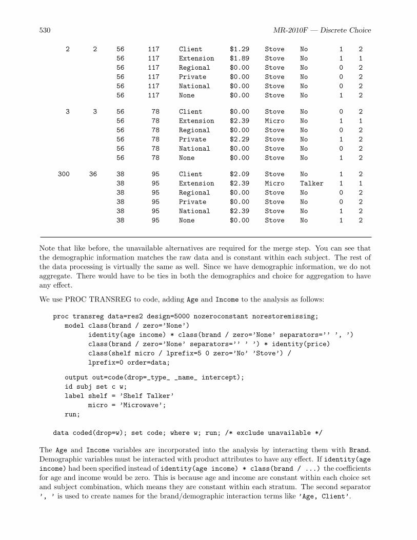
530 MR-2010F — Discrete Choice
2 2 56 117 Client $1.29 Stove No 1 256 117 Extension $1.89 Stove No 1 156 117 Regional $0.00 Stove No 0 256 117 Private $0.00 Stove No 0 256 117 National $0.00 Stove No 0 256 117 None $0.00 Stove No 1 2
3 3 56 78 Client $0.00 Stove No 0 256 78 Extension $2.39 Micro No 1 156 78 Regional $0.00 Stove No 0 256 78 Private $2.29 Stove No 1 256 78 National $0.00 Stove No 0 256 78 None $0.00 Stove No 1 2
300 36 38 95 Client $2.09 Stove No 1 238 95 Extension $2.39 Micro Talker 1 138 95 Regional $0.00 Stove No 0 238 95 Private $0.00 Stove No 0 238 95 National $2.39 Stove No 1 238 95 None $0.00 Stove No 1 2
Note that like before, the unavailable alternatives are required for the merge step. You can see thatthe demographic information matches the raw data and is constant within each subject. The rest ofthe data processing is virtually the same as well. Since we have demographic information, we do notaggregate. There would have to be ties in both the demographics and choice for aggregation to haveany effect.
We use PROC TRANSREG to code, adding Age and Income to the analysis as follows:
proc transreg data=res2 design=5000 nozeroconstant norestoremissing;model class(brand / zero=’None’)
identity(age income) * class(brand / zero=’None’ separators=’’ ’, ’)class(brand / zero=’None’ separators=’’ ’ ’) * identity(price)class(shelf micro / lprefix=5 0 zero=’No’ ’Stove’) /lprefix=0 order=data;
output out=code(drop=_type_ _name_ intercept);id subj set c w;label shelf = ’Shelf Talker’
micro = ’Microwave’;run;
data coded(drop=w); set code; where w; run; /* exclude unavailable */
The Age and Income variables are incorporated into the analysis by interacting them with Brand.Demographic variables must be interacted with product attributes to have any effect. If identity(ageincome) had been specified instead of identity(age income) * class(brand / ...) the coefficientsfor age and income would be zero. This is because age and income are constant within each choice setand subject combination, which means they are constant within each stratum. The second separator’, ’ is used to create names for the brand/demographic interaction terms like ’Age, Client’.

MR-2010F — Food Product Example with Asymmetry and Availability Cross-Effects 531
The following steps display the first coded choice set:
proc print data=coded(obs=4) label;id brand price;var BrandClient -- BrandPrivate Shelf Micro c;run;
proc print data=coded(obs=4 drop=Age) label;id brand price;var Age:;run;
proc print data=coded(obs=4 drop=Income) label;id brand price;var Income:;run;
proc print data=coded(obs=4) label;id brand price;var BrandClientPrice -- BrandPrivatePrice;format BrandClientPrice -- BrandPrivatePrice best4.;run;
The coded data set for the first subject and choice set is displayed next in a series of panels. The partthat is new is the second and third panel, which are used to capture the brand by age and brand byincome effects. The attributes and the brand effects are as follows:
Consumer Food Product Example
ShelfBrand Price Client Extension Regional Private Talker Microwave c
Client $1.29 1 0 0 0 No Stove 2Extension $2.39 0 1 0 0 No Micro 1Regional $1.99 0 0 1 0 No Stove 2National $1.99 0 0 0 0 No Stove 2

532 MR-2010F — Discrete Choice
The age by brand effects are as follows:
Consumer Food Product Example
Age, Age, Age, Age, Age,Brand Price Client Extension Regional Private National
Client $1.29 33 0 0 0 0Extension $2.39 0 33 0 0 0Regional $1.99 0 0 33 0 0National $1.99 0 0 0 0 33
The income by brand effects are as follows:
Consumer Food Product Example
Income, Income, Income, Income, Income,Brand Price Client Extension Regional Private National
Client $1.29 109 0 0 0 0Extension $2.39 0 109 0 0 0Regional $1.99 0 0 109 0 0National $1.99 0 0 0 0 109
The alternative-specific price effects are as follows:
Consumer Food Product Example
Client Extension Regional PrivateBrand Price Price Price Price Price
Client $1.29 1.29 0 0 0Extension $2.39 0 2.39 0 0Regional $1.99 0 0 1.99 0National $1.99 0 0 0 0
The PROC PHREG specification is the same as we have used before with nonaggregated data. Thefollowing step performs the analysis:
proc phreg data=coded brief;model c*c(2) = &_trgind / ties=breslow;strata subj set;run;

MR-2010F — Food Product Example with Asymmetry and Availability Cross-Effects 533
This step took just about one minute and produced the following results:
Consumer Food Product Example
The PHREG Procedure
Model Information
Data Set WORK.CODEDDependent Variable cCensoring Variable cCensoring Value(s) 2Ties Handling BRESLOW
Number of Observations Read 47400Number of Observations Used 47400
Summary of Subjects, Sets, and Chosen and Unchosen Alternatives
Number of Number of Chosen NotPattern Choices Alternatives Alternatives Chosen
1 2400 3 1 22 1800 4 1 33 6600 5 1 4
Convergence Status
Convergence criterion (GCONV=1E-8) satisfied.
Model Fit Statistics
Without WithCriterion Covariates Covariates
-2 LOG L 31508.579 10939.139AIC 31508.579 10983.139SBC 31508.579 11143.460
Testing Global Null Hypothesis: BETA=0
Test Chi-Square DF Pr > ChiSq
Likelihood Ratio 20569.4401 22 <.0001Score 21088.4411 22 <.0001Wald 6947.1766 22 <.0001

534 MR-2010F — Discrete Choice
Consumer Food Product Example
The PHREG Procedure
Multinomial Logit Parameter Estimates
Parameter StandardDF Estimate Error Chi-Square Pr > ChiSq
Client 1 2.04997 0.81287 6.3599 0.0117Extension 1 0.47882 0.81714 0.3434 0.5579Regional 1 -1.49923 1.51428 0.9802 0.3221Private 1 3.33861 0.85485 15.2528 <.0001National 1 -0.62955 1.06206 0.3514 0.5533Age, Client 1 0.01142 0.00944 1.4655 0.2261Age, Extension 1 0.00855 0.00949 0.8111 0.3678Age, Regional 1 0.01114 0.01205 0.8548 0.3552Age, Private 1 0.00826 0.00970 0.7247 0.3946Age, National 1 0.00809 0.00964 0.7042 0.4014
Income, Client 1 0.03227 0.00771 17.4954 <.0001Income, Extension 1 0.05717 0.00776 54.2991 <.0001Income, Regional 1 0.02496 0.01014 6.0642 0.0138Income, Private 1 0.00957 0.00794 1.4521 0.2282Income, National 1 0.00929 0.00789 1.3858 0.2391
Client Price 1 -0.76510 0.09598 63.5410 <.0001Extension Price 1 -0.51364 0.08465 36.8207 <.0001Regional Price 1 -0.27824 0.46406 0.3595 0.5488Private Price 1 -1.37957 0.14286 93.2538 <.0001National Price 1 0.82684 0.29260 7.9852 0.0047Shelf Talker 1 0.74026 0.07033 110.7751 <.0001Micro 1 0.59312 0.05692 108.6006 <.0001
In other examples, when we use the brief option to produce a brief summary of the strata, the tablehas only one line. In this case, since our choice sets have 3, 4, or 5 alternatives, we have three rows,one for each choice set size. The coefficients for the age and income variables are generally not verysignificant in this analysis except an effect for income on the client brand and particularly on theextension.

MR-2010F — Allocation of Prescription Drugs 535
Allocation of Prescription Drugs
This example discusses an allocation study, which is a technique often used in the area of prescriptiondrug marketing research. This example discusses designing the allocation experiment, processing thedata, analyzing frequencies, analyzing proportions, coding, analysis, and results. The principles ofdesigning an allocation study are the same as for designing a first-choice experiment, as is the codingand final analysis. However, processing the data before analysis is different.
The previous examples have all modeled simple choice. However, sometimes the response of interest isnot simple first choice. For example, in prescription drug marketing, researchers often use allocationstudies where multiple, not single choices are made. Physicians are asked questions like “For the nextten prescriptions you write for a particular condition, how many would you write for each of thesedrugs?” The response, for example, could be “5 for drug 1, none for drug 2, 3 for drug 3, and 2 fordrug 4.”
Designing the Allocation Experiment
In this study, physicians are asked to specify which of ten drugs they would prescribe to their nextten patients. In this study, ten drugs, Drug 1 — Drug 10, are available each at three different prices,$50, $75, and $100. In real studies, real brand names are used and there would probably be moreattributes. Since experimental design has been covered in some detail in other examples, we chose asimple design for this experiment so that we could concentrate on data processing. First, we use the%MktRuns autocall macro to suggest a design size. (All of the autocall macros used in this book aredocumented starting on page 803.) We specify 3 ** 10 for the 10 three-level factors as follows:
title ’Allocation of Prescription Drugs’;
%mktruns(3 ** 10)
The results are as follows:
Allocation of Prescription Drugs
Design Summary
Number ofLevels Frequency
3 10
Allocation of Prescription Drugs
Saturated = 21Full Factorial = 59,049

536 MR-2010F — Discrete Choice
Some Reasonable Cannot BeDesign Sizes Violations Divided By
27 * 036 * 045 * 054 * 021 S 45 924 45 930 45 933 45 939 45 942 45 9
* - 100% Efficient design can be made with the MktEx macro.S - Saturated Design - The smallest design that can be made.
Allocation of Prescription Drugs
n Design Reference
27 3 ** 13 Fractional-Factorial36 2 ** 11 3 ** 12 Orthogonal Array36 2 ** 4 3 ** 13 Orthogonal Array36 2 ** 2 3 ** 12 6 ** 1 Orthogonal Array36 3 ** 13 4 ** 1 Orthogonal Array36 3 ** 12 12 ** 1 Orthogonal Array45 3 ** 10 5 ** 1 Orthogonal Array54 2 ** 1 3 ** 25 Orthogonal Array54 2 ** 1 3 ** 21 9 ** 1 Orthogonal Array54 3 ** 24 6 ** 1 Orthogonal Array54 3 ** 20 6 ** 1 9 ** 1 Orthogonal Array54 3 ** 18 18 ** 1 Orthogonal Array
We need at least 21 choice sets and we see the optimal sizes are all divisible by nine. We use 27 choicesets, which can give us up to 13 three-level factors.
Next, we use the %MktEx macro to create the design.∗ In addition, one more factor is added to thedesign. This factor is used to block the design into three blocks of size 9. The following step generatesthe design:
%let nalts = 10;
%mktex(3 ** &nalts 3, n=27, seed=396)
∗Due to machine, SAS release, and macro differences, you might not get exactly the same design used in this book,but the differences should be slight.

MR-2010F — Allocation of Prescription Drugs 537
The macro finds a 100% D-efficient design. The results are as follows:
Allocation of Prescription Drugs
Algorithm Search History
Current BestDesign Row,Col D-Efficiency D-Efficiency Notes----------------------------------------------------------
1 Start 100.0000 100.0000 Tab1 End 100.0000
Allocation of Prescription Drugs
The OPTEX Procedure
Class Level Information
Class Levels -Values-
x1 3 1 2 3x2 3 1 2 3x3 3 1 2 3x4 3 1 2 3x5 3 1 2 3x6 3 1 2 3x7 3 1 2 3x8 3 1 2 3x9 3 1 2 3x10 3 1 2 3x11 3 1 2 3
Allocation of Prescription Drugs
The OPTEX Procedure
AveragePrediction
Design StandardNumber D-Efficiency A-Efficiency G-Efficiency Error------------------------------------------------------------------------
1 100.0000 100.0000 100.0000 0.9230
The %MktEx macro always creates factor names of x1, x2, and so on with values of 1, 2, .... You cancreate a data set with the names and values you want and use it to rename the factors and reset thelevels. This first step creates a data set with 11 variables, Block and Brand1 - Brand10. Block hasvalues 1, 2, and 3, and the brand variables have values of 50, 75, and 100 with a dollar format. The%MktLab macro takes the data=Randomized design data set and uses the names, values, and formats in

538 MR-2010F — Discrete Choice
the key=Key data set to make the out=Final data set. This data set is sorted by block and displayed.The %MktEval macro is called to check the results. The following steps process and evaluate the design:
data key(drop=i);input Block Brand1;array Brand[10];do i = 2 to 10; brand[i] = brand1; end;format brand: dollar4.;datalines;
1 502 753 100;
proc print; run;
%mktlab(data=randomized, key=key)
proc sort out=sasuser.DrugAlloLinDes; by block; run;
proc print; id block; by block; run;
%mkteval(blocks=block)
.
The key= data set is as follows:
Allocation of Prescription Drugs
Obs Block Brand1 Brand2 Brand3 Brand4 Brand5 Brand6 Brand7 Brand8 Brand9 Brand10
1 1 $50 $50 $50 $50 $50 $50 $50 $50 $50 $502 2 $75 $75 $75 $75 $75 $75 $75 $75 $75 $753 3 $100 $100 $100 $100 $100 $100 $100 $100 $100 $100
The %MktLab macro displays the following mapping information:

MR-2010F — Allocation of Prescription Drugs 539
Variable Mapping:x1 : Blockx2 : Brand1x3 : Brand2x4 : Brand3x5 : Brand4x6 : Brand5x7 : Brand6x8 : Brand7x9 : Brand8x10 : Brand9x11 : Brand10
The design is as follows:
Allocation of Prescription Drugs
Block Brand1 Brand2 Brand3 Brand4 Brand5 Brand6 Brand7 Brand8 Brand9 Brand10
1 $50 $75 $50 $75 $100 $100 $100 $100 $50 $100$100 $50 $100 $75 $75 $75 $100 $50 $100 $75$50 $50 $75 $100 $50 $75 $50 $75 $50 $75$75 $50 $50 $50 $100 $75 $75 $100 $75 $75$75 $75 $100 $100 $75 $100 $50 $50 $75 $100$50 $100 $100 $50 $75 $50 $75 $50 $50 $50$100 $75 $75 $50 $50 $100 $75 $75 $100 $100$100 $100 $50 $100 $100 $50 $50 $100 $100 $50$75 $100 $75 $75 $50 $50 $100 $75 $75 $50
2 $100 $75 $50 $100 $75 $50 $100 $75 $75 $75$100 $100 $100 $75 $50 $75 $75 $100 $75 $100$50 $75 $100 $50 $50 $50 $50 $100 $100 $75$75 $50 $100 $100 $50 $100 $100 $100 $50 $50$50 $100 $75 $100 $100 $75 $100 $50 $100 $100$100 $50 $75 $50 $100 $100 $50 $50 $75 $50$50 $50 $50 $75 $75 $100 $75 $75 $100 $50$75 $75 $75 $75 $100 $50 $75 $50 $50 $75$75 $100 $50 $50 $75 $75 $50 $75 $50 $100

540 MR-2010F — Discrete Choice
3 $100 $75 $100 $75 $100 $75 $50 $75 $50 $50$75 $75 $50 $50 $50 $75 $100 $50 $100 $50$50 $75 $75 $100 $75 $75 $75 $100 $75 $50$50 $100 $50 $75 $50 $100 $50 $50 $75 $75$50 $50 $100 $50 $100 $50 $100 $75 $75 $100$75 $50 $75 $75 $75 $50 $50 $100 $100 $100$75 $100 $100 $100 $100 $100 $75 $75 $100 $75
$100 $50 $50 $100 $50 $50 $75 $50 $50 $100$100 $100 $75 $50 $75 $100 $100 $100 $50 $75
Some of the evaluation results are as follows:
Allocation of Prescription DrugsCanonical Correlations Between the Factors
There are 0 Canonical Correlations Greater Than 0.316
Block Brand1 Brand2 Brand3 Brand4 Brand5 Brand6 Brand7 Brand8 Brand9 Brand10
Block 1 0 0 0 0 0 0 0 0 0 0Brand1 0 1 0 0 0 0 0 0 0 0 0Brand2 0 0 1 0 0 0 0 0 0 0 0Brand3 0 0 0 1 0 0 0 0 0 0 0Brand4 0 0 0 0 1 0 0 0 0 0 0Brand5 0 0 0 0 0 1 0 0 0 0 0Brand6 0 0 0 0 0 0 1 0 0 0 0Brand7 0 0 0 0 0 0 0 1 0 0 0Brand8 0 0 0 0 0 0 0 0 1 0 0Brand9 0 0 0 0 0 0 0 0 0 1 0Brand10 0 0 0 0 0 0 0 0 0 0 1
Allocation of Prescription DrugsSummary of Frequencies
There are 0 Canonical Correlations Greater Than 0.316
Frequencies
Block 9 9 9Brand1 9 9 9Brand2 9 9 9Brand3 9 9 9Brand4 9 9 9Brand5 9 9 9Brand6 9 9 9Brand7 9 9 9Brand8 9 9 9Brand9 9 9 9Brand10 9 9 9

MR-2010F — Allocation of Prescription Drugs 541
Block Brand1 3 3 3 3 3 3 3 3 3Block Brand2 3 3 3 3 3 3 3 3 3Block Brand3 3 3 3 3 3 3 3 3 3Block Brand4 3 3 3 3 3 3 3 3 3Block Brand5 3 3 3 3 3 3 3 3 3Block Brand6 3 3 3 3 3 3 3 3 3Block Brand7 3 3 3 3 3 3 3 3 3Block Brand8 3 3 3 3 3 3 3 3 3Block Brand9 3 3 3 3 3 3 3 3 3Block Brand10 3 3 3 3 3 3 3 3 3...N-Way 1 1 1 1 1 1 1 1 1 1 1 1 1 1 1 1 1 1 1
1 1 1 1 1 1 1 1
We can also create a choice design from the linear arrangement and evaluate it using the %ChoicEffmacro. The design is rolled into a choice design as follows using the same technique that we used inprevious examples:
%mktkey(Brand1-Brand10)
data key(keep=Brand Price);input Brand $ 1-8 Price $;datalines;
Brand 1 Brand1Brand 2 Brand2Brand 3 Brand3Brand 4 Brand4Brand 5 Brand5Brand 6 Brand6Brand 7 Brand7Brand 8 Brand8Brand 9 Brand9Brand 10 Brand10- .;
%mktroll(design=sasuser.DrugAlloLinDes, key=key, alt=brand, out=rolled,options=nowarn)
At this point, the choice design can be stored in a permanent SAS data set stored for analysis time aswe have done in previous examples. Alternatively, you an just store the linear arrangement and usethe same (or similar) code to make the choice design at analysis time. We use the latter approach here.This is because a form that is convenient for analysis is not always convenient for design evaluation.This is explained in more detail once the evaluation results are displayed. For now, simply note thatthe constant alternative is denoted by a dash here, but we use a blank (or character missing value) forthe analysis.

542 MR-2010F — Discrete Choice
The choice design is evaluated as follows:
%choiceff(data=rolled, /* candidate set of choice sets */init=rolled(keep=set), /* select these sets */intiter=0, /* evaluate without internal iterations */
/* model with stdz orthogonal coding *//* ref level for brand is ’-’ */
model=class(brand price / zero=’-’ sta),options=relative, /* display relative D-efficiency */nsets=27, /* number of choice sets */nalts=11, /* number of alternatives */beta=zero) /* assumed beta vector, Ho: b=0 */
Some of the results are as follows:
Allocation of Prescription Drugs
Final Results
Design 1Choice Sets 27Alternatives 11Parameters 12Maximum Parameters 270D-Efficiency 26.1557Relative D-Eff 96.8729D-Error 0.03821 / Choice Sets 0.0370
Allocation of Prescription Drugs
Standardn Variable Name Label Variance DF Error
1 BrandBrand__1 Brand Brand 1 0.037037 1 0.192452 BrandBrand__2 Brand Brand 2 0.037037 1 0.192453 BrandBrand__3 Brand Brand 3 0.037037 1 0.192454 BrandBrand__4 Brand Brand 4 0.037037 1 0.192455 BrandBrand__5 Brand Brand 5 0.037037 1 0.192456 BrandBrand__6 Brand Brand 6 0.037037 1 0.192457 BrandBrand__7 Brand Brand 7 0.037037 1 0.192458 BrandBrand__8 Brand Brand 8 0.037037 1 0.192459 BrandBrand__9 Brand Brand 9 0.037037 1 0.1924510 BrandBrand_10 Brand Brand 10 0.037037 1 0.1924511 Price50 Price 50 0.044815 1 0.2117012 Price75 Price 75 0.044815 1 0.21170
==12

MR-2010F — Allocation of Prescription Drugs 543
Note that there are 12 parameters, one of each of the 10 brands (10 brands minus plus one constant,minus 1) and two for price (three brands minus 1). The constant brand (not shown, but representedby ’-’) was explicitly designated as the reference level for brand. The standardized orthogonal contrastcoding is used for both attributes. Note that each of the 11 brands (including the constant) appearsin each of the 11 alternatives in each choice set, the variances for Brand are at the minimum value ofone over the number of choice sets. The price attribute does not have a perfect relationship like this,3 prices does not evenly divide 11 alternatives, and there is a constant alternative, so the variances forthe price attribute are higher. Still, they look pretty good. Relative D-efficiency is 96.8729, which ispretty good. Note that like before, relative D-efficiency = 100 is not possible since there is a constantalternative and 3 does not divide 11. So again, this design looks pretty good.
Processing the Data
Questionnaires are generated and data collected using a minor modification of the methods discussedin earlier examples. The difference is instead of asking for first choice data, allocation data are collectedinstead. Each row of the input data set contains a block, subject, and set number, followed by thenumber of times each of the ten alternatives is chosen. If all of the choice frequencies are zero, then theconstant alternative is chosen. The if statement is used to check data entry. For convenience, choiceset number is recoded to run from 1 to 27 instead of consisting of three blocks of nine sets. This givesus one fewer variable on which to stratify.
data results;input Block Subject Set @9 (freq1-freq&nalts) (2.);if not (sum(of freq:) in (0, &nalts)) then put _all_;set = (block - 1) * 9 + set;datalines;
1 1 1 0 0 8 0 2 0 0 0 0 01 1 2 0 0 8 0 0 0 2 0 0 01 1 3 0 0 0 0 0 0 0 010 01 1 4 1 0 0 1 3 3 0 0 2 01 1 5 2 0 8 0 0 0 0 0 0 01 1 6 0 1 3 1 0 0 0 0 1 41 1 7 0 1 3 1 1 2 0 0 2 01 1 8 0 0 3 0 0 2 1 0 0 41 1 9 0 2 5 0 0 0 0 0 3 02 210 1 1 0 2 0 3 0 1 1 12 211 1 0 3 1 0 1 1 0 2 1...;
In the first step, in creating an analysis data set for an allocation study, we reformat the data fromone row per choice set per block per subject (9× 3× 100 = 2700 observations) to one per alternative(including the constant) per choice set per block per subject ((10+1)×9×3×100 = 29, 700 observations).

544 MR-2010F — Discrete Choice
For each choice set, 11 observations are written storing the choice frequency in the variable Count andthe brand in the variable Brand. If no alternative is chosen, then the constant alternative is chosen tentimes, otherwise it is chosen zero times. The following steps process and display some of the data:
data allocs(keep=block set brand count);set results;array freq[&nalts];
* Handle the &nalts alternatives;do b = 1 to &nalts;
Brand = ’Brand ’ || put(b, 2.);Count = freq[b];output;end;
* Constant alt choice is implied if nothing else is chosen.brand = ’ ’ is used to flag the constant alternative.;
brand = ’ ’;count = 10 * (sum(of freq:) = 0);output;run;
proc print data=results(obs=3) label noobs; run;proc print data=allocs(obs=33); id block set; by block set; run;
The PROC PRINT steps show how the first three observations of the Results data set are transposedinto the first 33 observations of the Allocs data set. The results are as follows:
Allocation of Prescription Drugs
Block Subject Set Freq1 Freq2 Freq3 Freq4 Freq5 Freq6 Freq7 Freq8 Freq9 Freq10
1 1 1 0 0 8 0 2 0 0 0 0 01 1 2 0 0 8 0 0 0 2 0 0 01 1 3 0 0 0 0 0 0 0 0 10 0

MR-2010F — Allocation of Prescription Drugs 545
Allocation of Prescription Drugs
Block Set Brand Count
1 1 Brand 1 0Brand 2 0Brand 3 8Brand 4 0Brand 5 2Brand 6 0Brand 7 0Brand 8 0Brand 9 0Brand 10 0
0
1 2 Brand 1 0Brand 2 0Brand 3 8Brand 4 0Brand 5 0Brand 6 0Brand 7 2Brand 8 0Brand 9 0Brand 10 0
0
1 3 Brand 1 0Brand 2 0Brand 3 0Brand 4 0Brand 5 0Brand 6 0Brand 7 0Brand 8 0Brand 9 10Brand 10 0
0

546 MR-2010F — Discrete Choice
The following step aggregates the data:
* Aggregate, store the results back in count.;
proc summary data=allocs nway missing;class set brand;output sum(count)=Count out=allocs(drop=_type_ _freq_);run;
It stores in the variable Count the number of times each alternative of each choice set is chosen. Thiscreates a data set with 297 observations (3 blocks × 9 sets × 11 alternatives = 297).
These next steps prepare the design for analysis. We need to create a data set Key that describes howthe factors in our design are used for analysis. It contains all of the factor names, Brand1, Brand2, ...,Brand10. We can run the %MktKey macro to get these names for cutting and pasting into the programwithout typing them as follows:
%mktkey(Brand1-Brand10)
The %MktKey macro produced the following line:
Brand1 Brand2 Brand3 Brand4 Brand5 Brand6 Brand7 Brand8 Brand9 Brand10
The next step rolls out the experimental design data set to match the choice allocations data set. Thedata set is transposed from one row per choice set to one row per alternative per choice set. This dataset also has 297 observations. As we saw in previous examples, the %MktRoll macro can be used toprocess the design as follows:
data key(keep=Brand Price);input Brand $ 1-8 Price $;datalines;
Brand 1 Brand1Brand 2 Brand2Brand 3 Brand3Brand 4 Brand4Brand 5 Brand5Brand 6 Brand6Brand 7 Brand7Brand 8 Brand8Brand 9 Brand9Brand 10 Brand10. .;
%mktroll(design=sasuser.DrugAlloLinDes, key=key, alt=brand, out=rolled,options=nowarn)
proc print data=rolled(obs=11); format price dollar4.; run;

MR-2010F — Allocation of Prescription Drugs 547
The results are as follows:
Allocation of Prescription Drugs
Obs Set Brand Price
1 1 Brand 1 $502 1 Brand 2 $753 1 Brand 3 $504 1 Brand 4 $755 1 Brand 5 $1006 1 Brand 6 $1007 1 Brand 7 $1008 1 Brand 8 $1009 1 Brand 9 $50
10 1 Brand 10 $10011 1 .
Both data sets must be sorted the same way before they can be merged. The constant alternative,indicated by a missing brand, is last in the design choice set and hence is out of order. Missing mustcome before nonmissing for the merge. The order is correct in the Allocs data set since it is createdby PROC SUMMARY with Brand as a class variable. The following step sorts the data:
proc sort data=rolled; by set brand; run;
The data are merged along with error checking to ensure that the merge proceeded properly. Bothdata sets should have the same observations and Set and Brand variables, so the merge should be oneto one. The following steps merge the data and display a subset of the results:
data allocs2;merge allocs(in=flag1) rolled(in=flag2);by set brand;if flag1 ne flag2 then put ’ERROR: Merge is not 1 to 1.’;format price dollar4.;run;
proc print data=allocs2(obs=22);var brand price count;sum count;by notsorted set;id set;run;
In the aggregate and combined data set, we see how often each alternative is chosen for each choiceset. For example, in the first choice set, the constant alternative is chosen zero times, Brand 1 at $100was chosen 103 times, and so on. The 11 alternatives are chosen a total of 1000 times, 100 subjectstimes 10 choices each. The results are as follows:
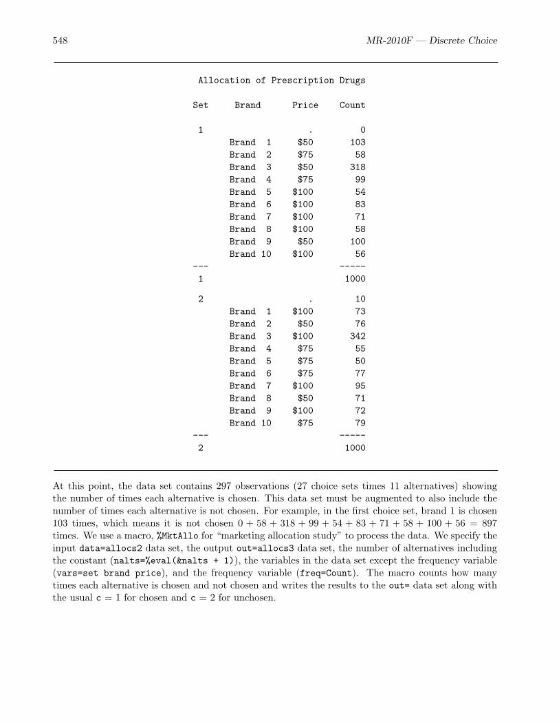
548 MR-2010F — Discrete Choice
Allocation of Prescription Drugs
Set Brand Price Count
1 . 0Brand 1 $50 103Brand 2 $75 58Brand 3 $50 318Brand 4 $75 99Brand 5 $100 54Brand 6 $100 83Brand 7 $100 71Brand 8 $100 58Brand 9 $50 100Brand 10 $100 56
--- -----1 1000
2 . 10Brand 1 $100 73Brand 2 $50 76Brand 3 $100 342Brand 4 $75 55Brand 5 $75 50Brand 6 $75 77Brand 7 $100 95Brand 8 $50 71Brand 9 $100 72Brand 10 $75 79
--- -----2 1000
At this point, the data set contains 297 observations (27 choice sets times 11 alternatives) showingthe number of times each alternative is chosen. This data set must be augmented to also include thenumber of times each alternative is not chosen. For example, in the first choice set, brand 1 is chosen103 times, which means it is not chosen 0 + 58 + 318 + 99 + 54 + 83 + 71 + 58 + 100 + 56 = 897times. We use a macro, %MktAllo for “marketing allocation study” to process the data. We specify theinput data=allocs2 data set, the output out=allocs3 data set, the number of alternatives includingthe constant (nalts=%eval(&nalts + 1)), the variables in the data set except the frequency variable(vars=set brand price), and the frequency variable (freq=Count). The macro counts how manytimes each alternative is chosen and not chosen and writes the results to the out= data set along withthe usual c = 1 for chosen and c = 2 for unchosen.
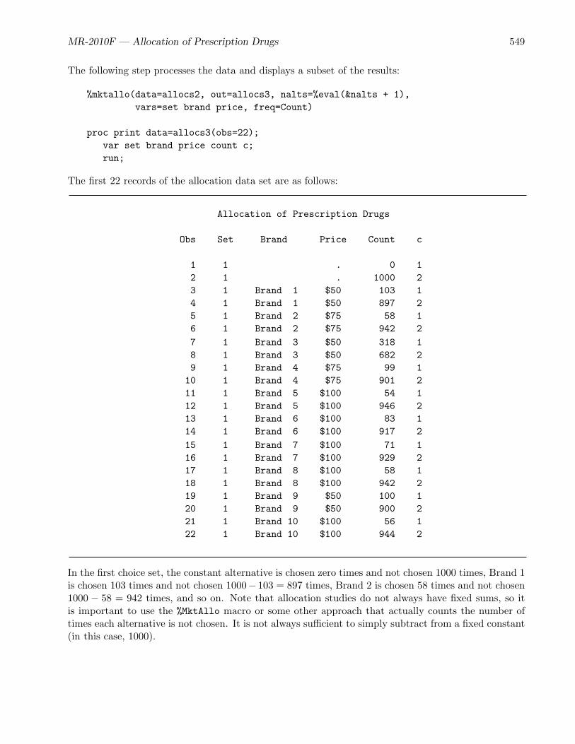
MR-2010F — Allocation of Prescription Drugs 549
The following step processes the data and displays a subset of the results:
%mktallo(data=allocs2, out=allocs3, nalts=%eval(&nalts + 1),vars=set brand price, freq=Count)
proc print data=allocs3(obs=22);var set brand price count c;run;
The first 22 records of the allocation data set are as follows:
Allocation of Prescription Drugs
Obs Set Brand Price Count c
1 1 . 0 12 1 . 1000 23 1 Brand 1 $50 103 14 1 Brand 1 $50 897 25 1 Brand 2 $75 58 16 1 Brand 2 $75 942 2
7 1 Brand 3 $50 318 18 1 Brand 3 $50 682 29 1 Brand 4 $75 99 110 1 Brand 4 $75 901 211 1 Brand 5 $100 54 112 1 Brand 5 $100 946 213 1 Brand 6 $100 83 114 1 Brand 6 $100 917 2
15 1 Brand 7 $100 71 116 1 Brand 7 $100 929 217 1 Brand 8 $100 58 118 1 Brand 8 $100 942 219 1 Brand 9 $50 100 120 1 Brand 9 $50 900 221 1 Brand 10 $100 56 122 1 Brand 10 $100 944 2
In the first choice set, the constant alternative is chosen zero times and not chosen 1000 times, Brand 1is chosen 103 times and not chosen 1000− 103 = 897 times, Brand 2 is chosen 58 times and not chosen1000 − 58 = 942 times, and so on. Note that allocation studies do not always have fixed sums, so itis important to use the %MktAllo macro or some other approach that actually counts the number oftimes each alternative is not chosen. It is not always sufficient to simply subtract from a fixed constant(in this case, 1000).

550 MR-2010F — Discrete Choice
Coding and Analysis
The next step codes the design for analysis. Indicator variables are created for Brand and Price. Allof the PROC TRANSREG options have been discussed in other examples. The following step does thecoding:
proc transreg design data=allocs3 nozeroconstant norestoremissing;model class(brand price / zero=none) / lprefix=0;output out=coded(drop=_type_ _name_ intercept);id set c count;run;
Analysis proceeds like it has in all other examples. We stratify by choice set number. We do not needto stratify by Block since choice set number does not repeat within block. The following step performsthe analysis:
proc phreg data=coded;where count > 0;model c*c(2) = &_trgind / ties=breslow;freq count;strata set;run;
We used the where statement to exclude observations with zero frequency; otherwise PROC PHREGcomplains about them.
Multinomial Logit Model Results
Recall that we used %phchoice(on) on page 287 to customize the output from PROC PHREG. Theresults are as follows:
Allocation of Prescription Drugs
The PHREG Procedure
Model Information
Data Set WORK.CODEDDependent Variable cCensoring Variable cCensoring Value(s) 2Frequency Variable CountTies Handling BRESLOW
Number of Observations Read 583Number of Observations Used 583Sum of Frequencies Read 297000Sum of Frequencies Used 297000

MR-2010F — Allocation of Prescription Drugs 551
Summary of Subjects, Sets, and Chosen and Unchosen Alternatives
Number of Chosen NotStratum Set Alternatives Alternatives Chosen
1 1 11000 1000 100002 2 11000 1000 100003 3 11000 1000 100004 4 11000 1000 100005 5 11000 1000 100006 6 11000 1000 100007 7 11000 1000 100008 8 11000 1000 100009 9 11000 1000 1000010 10 11000 1000 1000011 11 11000 1000 1000012 12 11000 1000 1000013 13 11000 1000 1000014 14 11000 1000 1000015 15 11000 1000 1000016 16 11000 1000 1000017 17 11000 1000 1000018 18 11000 1000 1000019 19 11000 1000 1000020 20 11000 1000 1000021 21 11000 1000 1000022 22 11000 1000 1000023 23 11000 1000 1000024 24 11000 1000 1000025 25 11000 1000 1000026 26 11000 1000 1000027 27 11000 1000 10000
---------------------------------------------------------------Total 297000 27000 270000
Convergence Status
Convergence criterion (GCONV=1E-8) satisfied.
Model Fit Statistics
Without WithCriterion Covariates Covariates
-2 LOG L 502505.13 489062.66AIC 502505.13 489086.66SBC 502505.13 489185.11

552 MR-2010F — Discrete Choice
Testing Global Null Hypothesis: BETA=0
Test Chi-Square DF Pr > ChiSq
Likelihood Ratio 13442.4676 12 <.0001Score 18340.8415 12 <.0001Wald 14087.6778 12 <.0001
Multinomial Logit Parameter Estimates
Parameter StandardDF Estimate Error Chi-Square Pr > ChiSq
Brand 1 1 2.09906 0.06766 962.5297 <.0001Brand 2 1 2.09118 0.06769 954.5113 <.0001Brand 3 1 3.54204 0.06484 2984.4698 <.0001Brand 4 1 2.09710 0.06766 960.5277 <.0001Brand 5 1 2.08523 0.06771 948.4791 <.0001Brand 6 1 2.03530 0.06790 898.6218 <.0001Brand 7 1 2.06920 0.06777 932.3154 <.0001Brand 8 1 2.08573 0.06771 948.9824 <.0001Brand 9 1 2.11705 0.06759 980.9640 <.0001Brand 10 1 2.06363 0.06779 926.7331 <.0001
$50 1 0.00529 0.01628 0.1058 0.7450$75 1 0.0005304 0.01629 0.0011 0.9740
$100 0 0 . . .
The output shows that there are 27 strata, one per choice set, each consisting of 1000 chosen alter-natives (10 choices by 100 subjects) and 10,000 unchosen alternatives. All of the brand coefficientsare “significant,” with the Brand 3 effect being by far the strongest. (We will soon see that statisticalsignificance should be ignored with allocation studies.) There is no price effect.
Analyzing Proportions
Recall that we collected data by asking physicians to report which brands they would prescribe thenext ten times they write prescriptions. Alternatively, we could ask them to report the proportion oftime they would prescribe each brand. We can simulate having proportion data by dividing our countdata by 10. This means our frequency variable no longer contains integers, so we need to specify thenotruncate option in the PROC PHREG freq statement to permit “noninteger frequencies.” This isillustrated in the following steps:
data coded2;set coded;count = count / 10;run;

MR-2010F — Allocation of Prescription Drugs 553
proc phreg data=coded2;where count > 0;model c*c(2) = &_trgind / ties=breslow;freq count / notruncate;strata set;run;
When we do this, we see the number of alternatives and the number chosen and not chosen decreaseby a factor of 10 as do all of the Chi-Square tests. The coefficients are unchanged. This implies thatmarket share calculations are invariant to the different scalings of the frequencies. However, the p-values are not invariant. The sample size is artificially inflated when counts are used so p-values arenot interpretable in an allocation study. When proportions are used, each subject is contributing 1 tothe number chosen instead of 10, just like a normal choice study, so p-values have meaning. The resultsare as follows:
Allocation of Prescription Drugs
The PHREG Procedure
Model Information
Data Set WORK.CODED2Dependent Variable cCensoring Variable cCensoring Value(s) 2Frequency Variable CountTies Handling BRESLOW
Number of Observations Read 583Number of Observations Used 583Sum of Frequencies Read 29700Sum of Frequencies Used 29700
Summary of Subjects, Sets, and Chosen and Unchosen Alternatives
Number of Chosen NotStratum Set Alternatives Alternatives Chosen
1 1 1100.0 100.0 1000.02 2 1100.0 100.0 1000.03 3 1100.0 100.0 1000.04 4 1100.0 100.0 1000.05 5 1100.0 100.0 1000.06 6 1100.0 100.0 1000.07 7 1100.0 100.0 1000.08 8 1100.0 100.0 1000.09 9 1100.0 100.0 1000.010 10 1100.0 100.0 1000.0

554 MR-2010F — Discrete Choice
11 11 1100.0 100.0 1000.012 12 1100.0 100.0 1000.013 13 1100.0 100.0 1000.014 14 1100.0 100.0 1000.015 15 1100.0 100.0 1000.016 16 1100.0 100.0 1000.017 17 1100.0 100.0 1000.018 18 1100.0 100.0 1000.019 19 1100.0 100.0 1000.020 20 1100.0 100.0 1000.021 21 1100.0 100.0 1000.022 22 1100.0 100.0 1000.023 23 1100.0 100.0 1000.024 24 1100.0 100.0 1000.025 25 1100.0 100.0 1000.026 26 1100.0 100.0 1000.027 27 1100.0 100.0 1000.0
---------------------------------------------------------------Total 29700.0 2700.0 27000.0
Convergence Status
Convergence criterion (GCONV=1E-8) satisfied.
Model Fit Statistics
Without WithCriterion Covariates Covariates
-2 LOG L 37816.553 36472.307AIC 37816.553 36496.307SBC 37816.553 36567.119
Testing Global Null Hypothesis: BETA=0
Test Chi-Square DF Pr > ChiSq
Likelihood Ratio 1344.2468 12 <.0001Score 1834.0841 12 <.0001Wald 1408.7678 12 <.0001
MR-2010F — Allocation of Prescription Drugs 555
Multinomial Logit Parameter Estimates
Parameter StandardDF Estimate Error Chi-Square Pr > ChiSq
Brand 1 1 2.09906 0.21395 96.2530 <.0001Brand 2 1 2.09118 0.21404 95.4511 <.0001Brand 3 1 3.54204 0.20503 298.4470 <.0001Brand 4 1 2.09710 0.21398 96.0528 <.0001Brand 5 1 2.08523 0.21411 94.8479 <.0001Brand 6 1 2.03530 0.21470 89.8622 <.0001Brand 7 1 2.06920 0.21430 93.2315 <.0001Brand 8 1 2.08573 0.21411 94.8982 <.0001Brand 9 1 2.11705 0.21375 98.0964 <.0001Brand 10 1 2.06363 0.21436 92.6733 <.0001
$50 1 0.00529 0.05148 0.0106 0.9181$75 1 0.0005304 0.05152 0.0001 0.9918$100 0 0 . . .

556 MR-2010F — Discrete Choice
Chair Design with Generic Attributes
This study illustrates creating an experimental design for a purely generic choice model. This examplediscusses generic attributes, alternative swapping, choice set swapping, and constant alternatives. Ina purely generic study, there are no brands, just bundles of attributes. Also see page 102 in theexperimental design chapter for examples of how to combinatorially construct optimal generic choicedesigns for certain problems. You can find additional examples in the documentation for the %ChoicEffmacro beginning on page 806.
Say a manufacturer is interested in designing one or more new chairs. The manufacturer can vary theattributes of the chairs, present subjects with competing chair designs, and model the effects of theattributes on choice. The attributes of interest are as follows:
Factor Attribute LevelsX1 Color 3 ColorsX2 Back 3 StylesX3 Seat 3 StylesX4 Arm Rest 3 StylesX5 Material 3 Materials
Since seeing descriptions of chairs is not the same as seeing and sitting in the actual chairs, themanufacturer is going to actually make sample chairs for people to try and choose from. Subjects areshown groups of three chairs at a time. If we were to make our design using the approach discussed inprevious examples, we would use the %MktEx autocall macro to create a design with 15 factors, five forthe first chair, five for the second chair, and five for the third chair. This design would need at least15 × (3 − 1) + 1 = 31 runs and 93 sample chairs. The following step shows how we could have madethe design:∗
title ’Generic Chair Attributes’;
* This design will not be used;%mktex(3 ** 15, n=36, seed=238)
%mktkey(3 5)
%mktroll(design=randomized, key=key, out=cand)
The %MktEx approach to designing an experiment like this allows you to fit very general models includingmodels with alternative-specific effects and even mother logit models. However, at analysis time for thispurely generic model, we fit a model with 10 parameters, two for each of the five factors, class(x1-x5).Creating a design with over 31× 3 = 93 chairs is way too expensive. In ordinary linear model designs,we need at least as many runs as parameters. In choice designs, we need to count the total numberof alternatives across all choice sets, subtract the number of choice sets, and this number must be atleast as large as the number of parameters. Equivalently, each choice set allows us to estimate m − 1parameters, where m is the number of alternatives in that choice set. In this case, we could fit ourpurely generic model with as few as 10/(3− 1) = 5 choice sets.
∗Due to machine, SAS release, and macro differences, you might not get exactly the same design used in this book,but the differences should be slight.

MR-2010F — Chair Design with Generic Attributes 557
Since we only need a simple generic model for this example, and since our chair manufacturing for ourresearch is expensive, we do not use the %MktEx approach for designing our choice experiment. Instead,we use a different approach that lets us get a smaller design that is adequate for our model and budget.Recall the discussion of linear model design efficiency, choice model design efficiency, and using linearmodel design efficiency as a surrogate for choice design goodness starting on page 62. Instead of usinglinear model design efficiency as a surrogate for choice design goodness, we can directly optimize choicedesign efficiency given an assumed model and parameter vector β. This approach uses the %ChoicEffmacro.
Generic Attributes, Alternative Swapping, Large Candidate Set
This part of the example illustrates using the %ChoicEff macro for efficient choice designs, using itsalgorithm that builds a design from candidate alternatives (as opposed to candidates consisting ofentire choice sets). First, we use the %MktRuns macro to suggest a candidate-set size as follows:
%mktruns(3 ** 5)
Some of the results are as follows:
Generic Chair Attributes
Design Summary
Number ofLevels Frequency
3 5
Saturated = 11Full Factorial = 243
Some Reasonable Cannot BeDesign Sizes Violations Divided By
18 * 027 * 036 * 012 10 915 10 921 10 924 10 930 10 933 10 911 S 15 3 9

558 MR-2010F — Discrete Choice
* - 100% Efficient design can be made with the MktEx macro.S - Saturated Design - The smallest design that can be made.
Note that the saturated design is not one of therecommended designs for this problem. It is shownto provide some context for the recommended sizes.
Generic Chair Attributes
n Design Reference
18 2 ** 1 3 ** 7 Orthogonal Array18 3 ** 6 6 ** 1 Orthogonal Array27 3 ** 13 Fractional-Factorial27 3 ** 9 9 ** 1 Fractional-Factorial36 2 ** 11 3 ** 12 Orthogonal Array36 2 ** 10 3 ** 8 6 ** 1 Orthogonal Array36 2 ** 4 3 ** 13 Orthogonal Array36 2 ** 3 3 ** 9 6 ** 1 Orthogonal Array36 2 ** 2 3 ** 12 6 ** 1 Orthogonal Array36 2 ** 2 3 ** 5 6 ** 2 Orthogonal Array36 2 ** 1 3 ** 8 6 ** 2 Orthogonal Array36 3 ** 13 4 ** 1 Orthogonal Array36 3 ** 12 12 ** 1 Orthogonal Array36 3 ** 7 6 ** 3 Orthogonal Array
We could use candidate sets of size: 18, 27 or 36. Additionally, since this problem is small, we couldtry an 81-run fractional-factorial design or the 243-run full-factorial design. We choose the 243-runfull-factorial design, since it is reasonably small and it gives the macro the most freedom to find a gooddesign.∗
We use the %MktEx macro to create a candidate set. The candidate set consists of 5 three-level factors,one for each of the five generic attributes. The following steps create the candidates:
%mktex(3 ** 5, n=243)
proc print data=design(obs=27); run;
Part of the candidate set is as follows:∗Later, we will see we could have chosen 18.
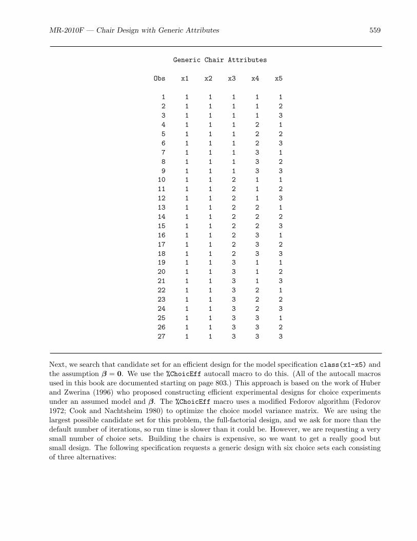
MR-2010F — Chair Design with Generic Attributes 559
Generic Chair Attributes
Obs x1 x2 x3 x4 x5
1 1 1 1 1 12 1 1 1 1 23 1 1 1 1 34 1 1 1 2 15 1 1 1 2 26 1 1 1 2 37 1 1 1 3 18 1 1 1 3 29 1 1 1 3 310 1 1 2 1 111 1 1 2 1 212 1 1 2 1 313 1 1 2 2 114 1 1 2 2 215 1 1 2 2 316 1 1 2 3 117 1 1 2 3 218 1 1 2 3 319 1 1 3 1 120 1 1 3 1 221 1 1 3 1 322 1 1 3 2 123 1 1 3 2 224 1 1 3 2 325 1 1 3 3 126 1 1 3 3 227 1 1 3 3 3
Next, we search that candidate set for an efficient design for the model specification class(x1-x5) andthe assumption β = 0. We use the %ChoicEff autocall macro to do this. (All of the autocall macrosused in this book are documented starting on page 803.) This approach is based on the work of Huberand Zwerina (1996) who proposed constructing efficient experimental designs for choice experimentsunder an assumed model and β. The %ChoicEff macro uses a modified Fedorov algorithm (Fedorov1972; Cook and Nachtsheim 1980) to optimize the choice model variance matrix. We are using thelargest possible candidate set for this problem, the full-factorial design, and we ask for more than thedefault number of iterations, so run time is slower than it could be. However, we are requesting a verysmall number of choice sets. Building the chairs is expensive, so we want to get a really good butsmall design. The following specification requests a generic design with six choice sets each consistingof three alternatives:

560 MR-2010F — Discrete Choice
%choiceff(data=design, /* candidate set of alternatives */model=class(x1-x5 / sta), /* model with stdzd orthogonal coding */nsets=6, /* number of choice sets */maxiter=100, /* maximum number of designs to make */seed=121, /* random number seed */flags=3, /* 3 alternatives, generic candidates */options=relative, /* display relative D-efficiency */beta=zero) /* assumed beta vector, Ho: b=0 */
The data=final option names the input data set of candidates. The model=class(x1-x5 / sta)option specifies the most general model that is considered at analysis time. This is a main-effectsmodel for x1-x5 with a standardized orthogonal contrast coding. You must specify this coding if youwant to see relative D-efficiency on a 0 to 100 scale. The nsets=6 option specifies the number of choicesets. Note that this is considerably smaller than the minimum of 31 that is required if we are justusing the %MktEx linear-arrangement approach (6× 3 = 18 chairs instead of 31× 3 = 93 chairs). Themaxiter=100 option requests 100 designs based on 100 random initial designs (by default, maxiter=2).The seed=121 option specifies the random number seed. The flags=3 option specifies that thereare three alternatives in a purely generic design.† The options=relative option scales D-efficiencyrelative to the hypothetical maximum value so that we can get a 0 to 100 scale for D-efficiency. RelativeD-efficiency is not displayed by default since it is only meaningful for some designs. The beta=zerooption specifies the assumption β = 0. A vector of numbers like beta=-1 0 -1 0 -1 0 -1 0 -1 0 -10 could be specified. (See page 878 for an example of this.) When you wish to assume all parametersare zero, you can specify beta=zero instead of typing a vector of the zeros. You can also omit thebeta= option if you just want the macro to list the parameters. You can use this list to ensure thatyou specify the parameters in the right order.
The first part of the output from the macro is a list of all of the effects generated and the assumedvalues of β. The effects are as follows:
Generic Chair Attributes
n Name Beta Label
1 x11 0 x1 12 x12 0 x1 23 x21 0 x2 14 x22 0 x2 25 x31 0 x3 16 x32 0 x3 27 x41 0 x4 18 x42 0 x4 29 x51 0 x5 110 x52 0 x5 2
†The option name flags= comes from the fact that in the context of other types of designs (designs with brands orlabeled alternatives), this option provides a set of “flag” variables that specify which candidates can be be used for whichalternatives.

MR-2010F — Chair Design with Generic Attributes 561
It is very important that you check this list and make sure it is correct. In particular, when you areexplicitly specifying the β vector, you need to make sure you specified all of the values in the rightorder. If you are not specifying a beta vector you can check the names and labels in the final table ofvariances and standard errors.
Next, the macro produces the iteration history, which is different from the iteration histories we areused to seeing in the %MktEx macro. The %ChoicEff macro uses PROC IML and a modified Fedorovalgorithm to iteratively improve the efficiency of the choice design given the specified candidates, model,and β. Note that these unscaled efficiencies are not on a 0 to 100 scale. This step took about 2 minutes.Some of the results are as follows:
Generic Chair Attributes
Design Iteration D-Efficiency D-Error----------------------------------------------
1 0 1.83063 * 0.546261 4.91557 * 0.203442 5.20220 * 0.192233 5.40987 * 0.184854 5.42657 * 0.18428
.
.
.
Design Iteration D-Efficiency D-Error----------------------------------------------
34 0 2.44100 0.409671 4.77565 0.209402 5.49875 0.181863 6.00000 * 0.166674 6.00000 0.16667
.
.
.
Design Iteration D-Efficiency D-Error----------------------------------------------
100 0 2.37105 0.421751 5.22899 0.191242 5.41804 0.184573 5.41804 0.18457
An asterisk is used to indicate places where D-efficiency is greater than any previously reported value.
Next, the macro shows which design it chose and the final D-efficiency and D-error (D-efficiency = 1 /D-error). The results are as follows:

562 MR-2010F — Discrete Choice
Generic Chair Attributes
Final Results
Design 34Choice Sets 6Alternatives 3Parameters 10Maximum Parameters 12D-Efficiency 6.0000Relative D-Eff 100.0000D-Error 0.16671 / Choice Sets 0.1667
Next, it shows the variance, standard error, and df for each effect as follows:
Generic Chair Attributes
Variable Standardn Name Label Variance DF Error
1 x11 x1 1 0.16667 1 0.408252 x12 x1 2 0.16667 1 0.408253 x21 x2 1 0.16667 1 0.408254 x22 x2 2 0.16667 1 0.408255 x31 x3 1 0.16667 1 0.408256 x32 x3 2 0.16667 1 0.408257 x41 x4 1 0.16667 1 0.408258 x42 x4 2 0.16667 1 0.408259 x51 x5 1 0.16667 1 0.4082510 x52 x5 2 0.16667 1 0.40825
==10
It is important to ensure that each effect is estimable: (df = 1). Usually, when all of the variances areconstant, like we see in this table, it means that the macro has found the optimal design. In fact, inthis case, we see that all of the variances in the last table equal both D-Error and one over the numberof choice sets in the preceding table. This means that relative D efficiency, which is also shown in thepreceding table must equal 100. With the standardized orthogonal contrast coding, and a situation likethis where an optimal design is possible, D-efficiency ranges from 0 to the number of choice sets. In theoptimal design, D-efficiency = 6, the number of sets, and relative D-efficiency is 100 times D-efficiencydivided by the number of choice sets.

MR-2010F — Chair Design with Generic Attributes 563
The data set Best contains the final, best design found. It is displayed as follows:
proc print; by set; id set; run;
The data set contains: Design – the number of the design with the maximum D-efficiency,Efficiency – the D-efficiency of this design,Index – the candidate set observation number,Set – the choice set number,Prob – the probability that this alternative will be chosen given β,n – the observation number,x1-x5 – the design, andf1- f3 – the automatically generated alternative flags.The data set is as follows:
Generic Chair Attributes
Set Design Efficiency Index Prob n x1 x2 x3 x4 x5 _f1 _f2 _f3
1 34 6 183 0.33333 595 3 1 3 1 3 1 1 134 6 62 0.33333 596 1 3 1 3 2 1 1 134 6 121 0.33333 597 2 2 2 2 1 1 1 1
2 34 6 217 0.33333 598 3 3 1 1 1 1 1 134 6 45 0.33333 599 1 2 2 3 3 1 1 134 6 104 0.33333 600 2 1 3 2 2 1 1 1
3 34 6 215 0.33333 601 3 2 3 3 2 1 1 134 6 147 0.33333 602 2 3 2 1 3 1 1 134 6 4 0.33333 603 1 1 1 2 1 1 1 1
4 34 6 78 0.33333 604 1 3 3 2 3 1 1 134 6 178 0.33333 605 3 1 2 3 1 1 1 134 6 110 0.33333 606 2 2 1 1 2 1 1 1
5 34 6 90 0.33333 607 2 1 1 3 3 1 1 134 6 46 0.33333 608 1 2 3 1 1 1 1 134 6 230 0.33333 609 3 3 2 2 2 1 1 1
6 34 6 195 0.33333 610 3 2 1 2 3 1 1 134 6 11 0.33333 611 1 1 2 1 2 1 1 134 6 160 0.33333 612 2 3 3 3 1 1 1 1
This design has 18 runs (6 choice sets × 3 alternatives). Notice that in this design, each level occursexactly once in each factor and each choice set. To use this design for analysis, you only need thevariables Set and x1-x5. Since it is already in choice design format, it does not need to be processedusing the %MktRoll macro. Since data collection, processing, and analysis have already been coveredin detail in other examples, this example concentrates solely on experimental design.
564 MR-2010F — Discrete Choice
There is one more test that should be run before a design is used. The %MktDups macro checks thedesign to see if any choice sets are duplicates of any other choice sets. The following steps evaluate thedesign:
%mktdups(generic, data=best, nalts=3, factors=x1-x5)
The results are as follows:
Design: GenericFactors: x1-x5
x1 x2 x3 x4 x5Sets w Dup Alts: 0Duplicate Sets: 0
The first line of the table tells us that this is a generic design. The second line tells us the factors asspecified in the factors= option. These are followed by the actual variable names for the factors. Thenext line reports the number of choice sets that have duplicate alternatives—that is, the number oftimes an alternative appears in a set more than once. The last line reports the number of duplicatechoice sets. In this case, there are no duplicates of either type. If there are duplicates, then changingthe random number seed might help. Changing other aspects of the design or the approach for makingthe design might help as well.
Generic Attributes, Alternative Swapping, Small Candidate Set
In this part of this example, we try to make an equivalent design to the one we just made, only thistime using a smaller candidate set. The following steps create and evaluate the design:
%mktex(3 ** 5, n=18)
%choiceff(data=design, /* candidate set of alternatives */model=class(x1-x5 / sta), /* model with stdzd orthogonal coding */nsets=6, /* number of choice sets */maxiter=20, /* maximum number of designs to make */seed=121, /* random number seed */flags=3, /* 3 alternatives, generic candidates */options=relative, /* display relative D-efficiency */beta=zero) /* assumed beta vector, Ho: b=0 */
proc print; by set; id set; run;
%mktdups(generic, data=best, nalts=3, factors=x1-x5)
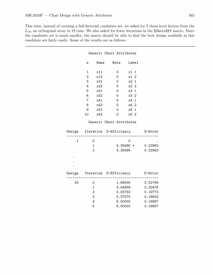
MR-2010F — Chair Design with Generic Attributes 565
This time, instead of creating a full-factorial candidate set, we asked for 5 three-level factors from theL18, an orthogonal array in 18 runs. We also asked for fewer iterations in the %ChoicEff macro. Sincethe candidate set is much smaller, the macro should be able to find the best design available in thiscandidate set fairly easily. Some of the results are as follows:
Generic Chair Attributes
n Name Beta Label
1 x11 0 x1 12 x12 0 x1 23 x21 0 x2 14 x22 0 x2 25 x31 0 x3 16 x32 0 x3 27 x41 0 x4 18 x42 0 x4 29 x51 0 x5 110 x52 0 x5 2
Generic Chair Attributes
Design Iteration D-Efficiency D-Error----------------------------------------------
1 0 0 .1 4.35495 * 0.229622 4.35495 0.22962
.
.
.
Design Iteration D-Efficiency D-Error----------------------------------------------
20 0 1.89505 0.527691 4.44909 0.224762 5.05750 0.197733 5.37575 0.186024 6.00000 0.166675 6.00000 0.16667

566 MR-2010F — Discrete Choice
Generic Chair Attributes
Final Results
Design 4Choice Sets 6Alternatives 3Parameters 10Maximum Parameters 12D-Efficiency 6.0000Relative D-Eff 100.0000D-Error 0.16671 / Choice Sets 0.1667
Generic Chair Attributes
Variable Standardn Name Label Variance DF Error
1 x11 x1 1 0.16667 1 0.408252 x12 x1 2 0.16667 1 0.408253 x21 x2 1 0.16667 1 0.408254 x22 x2 2 0.16667 1 0.408255 x31 x3 1 0.16667 1 0.408256 x32 x3 2 0.16667 1 0.408257 x41 x4 1 0.16667 1 0.408258 x42 x4 2 0.16667 1 0.408259 x51 x5 1 0.16667 1 0.4082510 x52 x5 2 0.16667 1 0.40825
==10
Generic Chair Attributes
Set Design Efficiency Index Prob n f1 f2 f3 x1 x2 x3 x4 x5
1 4 6 18 0.33333 55 1 1 1 3 3 3 3 34 6 1 0.33333 56 1 1 1 1 1 1 1 14 6 9 0.33333 57 1 1 1 2 2 2 2 2
2 4 6 3 0.33333 58 1 1 1 1 2 1 3 34 6 12 0.33333 59 1 1 1 2 3 2 1 14 6 14 0.33333 60 1 1 1 3 1 3 2 2
3 4 6 15 0.33333 61 1 1 1 3 2 1 2 14 6 8 0.33333 62 1 1 1 2 1 3 1 34 6 5 0.33333 63 1 1 1 1 3 2 3 2
4 4 6 16 0.33333 64 1 1 1 3 2 2 1 34 6 6 0.33333 65 1 1 1 1 3 3 2 14 6 7 0.33333 66 1 1 1 2 1 1 3 2
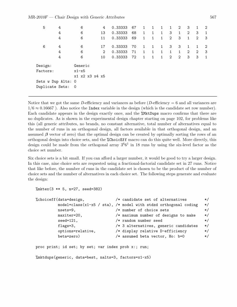
MR-2010F — Chair Design with Generic Attributes 567
5 4 6 4 0.33333 67 1 1 1 1 2 3 1 24 6 13 0.33333 68 1 1 1 3 1 2 3 14 6 11 0.33333 69 1 1 1 2 3 1 2 3
6 4 6 17 0.33333 70 1 1 1 3 3 1 1 24 6 2 0.33333 71 1 1 1 1 1 2 2 34 6 10 0.33333 72 1 1 1 2 2 3 3 1
Design: GenericFactors: x1-x5
x1 x2 x3 x4 x5Sets w Dup Alts: 0Duplicate Sets: 0
Notice that we got the same D-efficiency and variances as before (D-efficiency = 6 and all variances are1/6 ≈ 0.16667 ). Also notice the Index variable in the design (which is the candidate set row number).Each candidate appears in the design exactly once, and the %MktDups macro confirms that there areno duplicates. As is shown in the experimental design chapter starting on page 102, for problems likethis (all generic attributes, no brands, no constant alternative, total number of alternatives equal tothe number of runs in an orthogonal design, all factors available in that orthogonal design, and anassumed β vector of zero) that the optimal design can be created by optimally sorting the rows of anorthogonal design into choice sets, and the %ChoicEff macro can do this quite well. More directly, thisdesign could be made from the orthogonal array 3661 in 18 runs by using the six-level factor as thechoice set number.
Six choice sets is a bit small. If you can afford a larger number, it would be good to try a larger design.In this case, nine choice sets are requested using a fractional-factorial candidate set in 27 runs. Noticethat like before, the number of runs in the candidate set is chosen to be the product of the number ofchoice sets and the number of alternatives in each choice set. The following steps generate and evaluatethe design:
%mktex(3 ** 5, n=27, seed=382)
%choiceff(data=design, /* candidate set of alternatives */model=class(x1-x5 / sta), /* model with stdzd orthogonal coding */nsets=9, /* number of choice sets */maxiter=20, /* maximum number of designs to make */seed=121, /* random number seed */flags=3, /* 3 alternatives, generic candidates */options=relative, /* display relative D-efficiency */beta=zero) /* assumed beta vector, Ho: b=0 */
proc print; id set; by set; var index prob x:; run;
%mktdups(generic, data=best, nalts=3, factors=x1-x5)
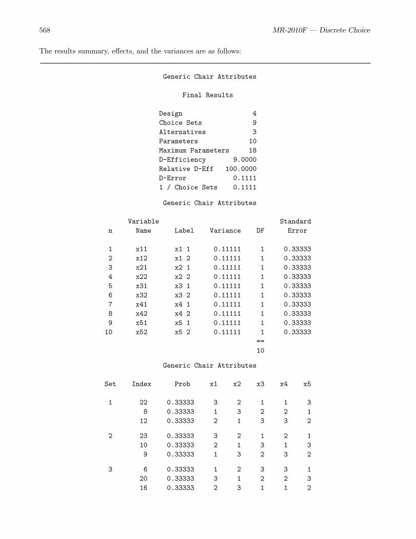
568 MR-2010F — Discrete Choice
The results summary, effects, and the variances are as follows:
Generic Chair Attributes
Final Results
Design 4Choice Sets 9Alternatives 3Parameters 10Maximum Parameters 18D-Efficiency 9.0000Relative D-Eff 100.0000D-Error 0.11111 / Choice Sets 0.1111
Generic Chair Attributes
Variable Standardn Name Label Variance DF Error
1 x11 x1 1 0.11111 1 0.333332 x12 x1 2 0.11111 1 0.333333 x21 x2 1 0.11111 1 0.333334 x22 x2 2 0.11111 1 0.333335 x31 x3 1 0.11111 1 0.333336 x32 x3 2 0.11111 1 0.333337 x41 x4 1 0.11111 1 0.333338 x42 x4 2 0.11111 1 0.333339 x51 x5 1 0.11111 1 0.3333310 x52 x5 2 0.11111 1 0.33333
==10
Generic Chair Attributes
Set Index Prob x1 x2 x3 x4 x5
1 22 0.33333 3 2 1 1 38 0.33333 1 3 2 2 112 0.33333 2 1 3 3 2
2 23 0.33333 3 2 1 2 110 0.33333 2 1 3 1 39 0.33333 1 3 2 3 2
3 6 0.33333 1 2 3 3 120 0.33333 3 1 2 2 316 0.33333 2 3 1 1 2

MR-2010F — Chair Design with Generic Attributes 569
4 13 0.33333 2 2 2 1 126 0.33333 3 3 3 2 23 0.33333 1 1 1 3 3
5 24 0.33333 3 2 1 3 27 0.33333 1 3 2 1 311 0.33333 2 1 3 2 1
6 14 0.33333 2 2 2 2 227 0.33333 3 3 3 3 31 0.33333 1 1 1 1 1
7 15 0.33333 2 2 2 3 325 0.33333 3 3 3 1 12 0.33333 1 1 1 2 2
8 21 0.33333 3 1 2 3 117 0.33333 2 3 1 2 34 0.33333 1 2 3 1 2
9 5 0.33333 1 2 3 2 318 0.33333 2 3 1 3 119 0.33333 3 1 2 1 2
Design: GenericFactors: x1-x5
x1 x2 x3 x4 x5Sets w Dup Alts: 0Duplicate Sets: 0
Notice that like before, the variances are constant, but in this case smaller at 1/9, and each candidateappears once. This is an optimal design in 9 choice sets. More directly, this design could be made fromthe orthogonal array 3991 in 27 runs by using the nine-level factor as the choice set number.
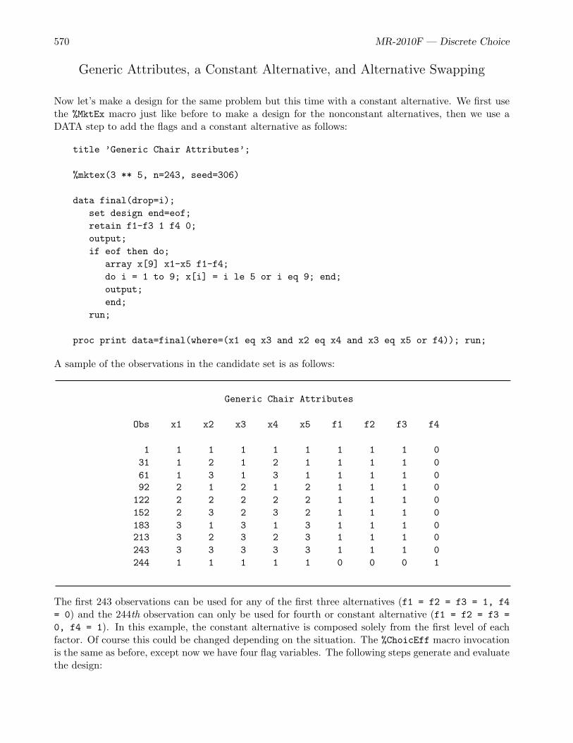
570 MR-2010F — Discrete Choice
Generic Attributes, a Constant Alternative, and Alternative Swapping
Now let’s make a design for the same problem but this time with a constant alternative. We first usethe %MktEx macro just like before to make a design for the nonconstant alternatives, then we use aDATA step to add the flags and a constant alternative as follows:
title ’Generic Chair Attributes’;
%mktex(3 ** 5, n=243, seed=306)
data final(drop=i);set design end=eof;retain f1-f3 1 f4 0;output;if eof then do;
array x[9] x1-x5 f1-f4;do i = 1 to 9; x[i] = i le 5 or i eq 9; end;output;end;
run;
proc print data=final(where=(x1 eq x3 and x2 eq x4 and x3 eq x5 or f4)); run;
A sample of the observations in the candidate set is as follows:
Generic Chair Attributes
Obs x1 x2 x3 x4 x5 f1 f2 f3 f4
1 1 1 1 1 1 1 1 1 031 1 2 1 2 1 1 1 1 061 1 3 1 3 1 1 1 1 092 2 1 2 1 2 1 1 1 0122 2 2 2 2 2 1 1 1 0152 2 3 2 3 2 1 1 1 0183 3 1 3 1 3 1 1 1 0213 3 2 3 2 3 1 1 1 0243 3 3 3 3 3 1 1 1 0244 1 1 1 1 1 0 0 0 1
The first 243 observations can be used for any of the first three alternatives (f1 = f2 = f3 = 1, f4= 0) and the 244th observation can only be used for fourth or constant alternative (f1 = f2 = f3 =0, f4 = 1). In this example, the constant alternative is composed solely from the first level of eachfactor. Of course this could be changed depending on the situation. The %ChoicEff macro invocationis the same as before, except now we have four flag variables. The following steps generate and evaluatethe design:
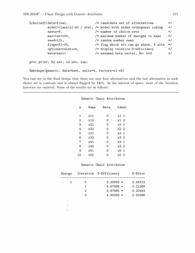
MR-2010F — Chair Design with Generic Attributes 571
%choiceff(data=final, /* candidate set of alternatives */model=class(x1-x5 / sta), /* model with stdzd orthogonal coding */nsets=6, /* number of choice sets */maxiter=100, /* maximum number of designs to make */seed=121, /* random number seed */flags=f1-f4, /* flag which alt can go where, 4 alts */options=relative, /* display relative D-efficiency */beta=zero) /* assumed beta vector, Ho: b=0 */
proc print; by set; id set; run;
%mktdups(generic, data=best, nalts=4, factors=x1-x5)
You can see in the final design that there are now four alternatives and the last alternative in eachchoice set is constant and is always flagged by f4=1. In the interest of space, most of the iterationhistories are omitted. Some of the results are as follows:
Generic Chair Attributes
n Name Beta Label
1 x11 0 x1 12 x12 0 x1 23 x21 0 x2 14 x22 0 x2 25 x31 0 x3 16 x32 0 x3 27 x41 0 x4 18 x42 0 x4 29 x51 0 x5 110 x52 0 x5 2
Generic Chair Attributes
Design Iteration D-Efficiency D-Error----------------------------------------------
1 0 2.20693 * 0.453121 4.67998 * 0.213682 4.87965 * 0.204933 4.90282 * 0.20396
.
.
.

572 MR-2010F — Discrete Choice
Design Iteration D-Efficiency D-Error----------------------------------------------
13 0 2.56694 0.389571 4.54049 0.220242 4.75518 0.210303 4.99035 0.200394 5.19495 * 0.192495 5.21381 * 0.19180
.
.
.
Design Iteration D-Efficiency D-Error----------------------------------------------
100 0 2.74564 0.364211 4.59264 0.217742 4.80304 0.208203 4.88340 0.20478
Generic Chair Attributes
Final Results
Design 13Choice Sets 6Alternatives 4Parameters 10Maximum Parameters 18D-Efficiency 5.2138Relative D-Eff 86.8968D-Error 0.19181 / Choice Sets 0.1667
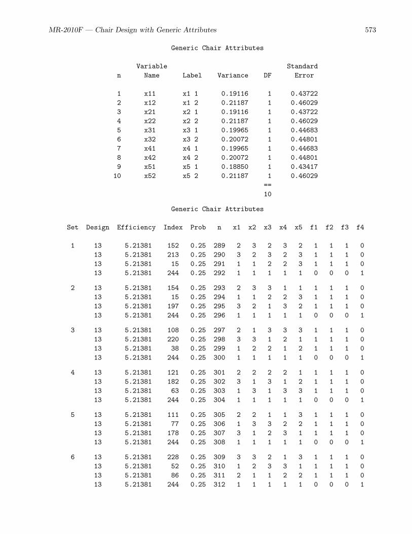
MR-2010F — Chair Design with Generic Attributes 573
Generic Chair Attributes
Variable Standardn Name Label Variance DF Error
1 x11 x1 1 0.19116 1 0.437222 x12 x1 2 0.21187 1 0.460293 x21 x2 1 0.19116 1 0.437224 x22 x2 2 0.21187 1 0.460295 x31 x3 1 0.19965 1 0.446836 x32 x3 2 0.20072 1 0.448017 x41 x4 1 0.19965 1 0.446838 x42 x4 2 0.20072 1 0.448019 x51 x5 1 0.18850 1 0.4341710 x52 x5 2 0.21187 1 0.46029
==10
Generic Chair Attributes
Set Design Efficiency Index Prob n x1 x2 x3 x4 x5 f1 f2 f3 f4
1 13 5.21381 152 0.25 289 2 3 2 3 2 1 1 1 013 5.21381 213 0.25 290 3 2 3 2 3 1 1 1 013 5.21381 15 0.25 291 1 1 2 2 3 1 1 1 013 5.21381 244 0.25 292 1 1 1 1 1 0 0 0 1
2 13 5.21381 154 0.25 293 2 3 3 1 1 1 1 1 013 5.21381 15 0.25 294 1 1 2 2 3 1 1 1 013 5.21381 197 0.25 295 3 2 1 3 2 1 1 1 013 5.21381 244 0.25 296 1 1 1 1 1 0 0 0 1
3 13 5.21381 108 0.25 297 2 1 3 3 3 1 1 1 013 5.21381 220 0.25 298 3 3 1 2 1 1 1 1 013 5.21381 38 0.25 299 1 2 2 1 2 1 1 1 013 5.21381 244 0.25 300 1 1 1 1 1 0 0 0 1
4 13 5.21381 121 0.25 301 2 2 2 2 1 1 1 1 013 5.21381 182 0.25 302 3 1 3 1 2 1 1 1 013 5.21381 63 0.25 303 1 3 1 3 3 1 1 1 013 5.21381 244 0.25 304 1 1 1 1 1 0 0 0 1
5 13 5.21381 111 0.25 305 2 2 1 1 3 1 1 1 013 5.21381 77 0.25 306 1 3 3 2 2 1 1 1 013 5.21381 178 0.25 307 3 1 2 3 1 1 1 1 013 5.21381 244 0.25 308 1 1 1 1 1 0 0 0 1
6 13 5.21381 228 0.25 309 3 3 2 1 3 1 1 1 013 5.21381 52 0.25 310 1 2 3 3 1 1 1 1 013 5.21381 86 0.25 311 2 1 1 2 2 1 1 1 013 5.21381 244 0.25 312 1 1 1 1 1 0 0 0 1

574 MR-2010F — Discrete Choice
Design: GenericFactors: x1-x5
x1 x2 x3 x4 x5Sets w Dup Alts: 0Duplicate Sets: 0
When there are three alternatives, each alternative has a probability of choice of 1/3, and now withfour alternatives, the probability is 1/4. They are all equal because of the assumption β = 0. Withother assumptions about β, typically the probabilities will not all be equal. Relative D-efficiency is lessthan 100 since there is a constant alternative. It must also be less than 100 since we have all three-levelfactors but four alternatives. The optimal D-efficiency is not the number of choice sets in designs likethis, so relative D-efficiency is less than 100.
To use this design for analysis, you only need the variables Set and x1-x5. Since it is already inchoice design format (one row per alternative), it does not need to be processed using the %MktRollmacro. Note that when you make designs with the %ChoicEff macro, the model statement in PROCTRANSREG should match or be no more complicated than the model specification that generated thedesign:
model class(x1-x5);
A model with fewer degrees of freedom is safe, although the design is suboptimal. For example, ifx1-x5 are quantitative attributes, the following model is safe:
model identity(x1-x5);
However, specifying interactions, or using this design in a branded study and specifying alternative-specific effects like this could lead to quite a few inestimable parameters. The following statementsillustrate:
* Bad idea for this design!!;model class(x1-x5 x1*x2 x4*x5);
* Another bad idea for this design!!;model class(brand)
class(brand * x1 brand * x2 brand * x3 brand * x4 brand * x5);
Generic Attributes, a Constant Alternative, and Choice Set Swapping
The %ChoicEff macro can be used in a very different way. Instead of providing a candidate setof alternatives to swap in and out of the design, you can provide a candidate set of entire choicesets. For this particular example, swapping alternatives is almost certainly better (see page 579).However, sometimes, if you need to impose restrictions on which alternative can appear with whichother alternative, then you must use the set-swapping options. We start by using the %MktEx macroto make a candidate design, with one run per choice set and one factor for each attribute of eachalternative (just like we did in the vacation, fabric softener, and food examples). We then process thecandidates from one row per choice set to one row per alternative per choice set using the %MktRoll

MR-2010F — Chair Design with Generic Attributes 575
macro. The following steps make the candidate set of choice sets:
%mktex(3 ** 15, n=81 * 81, seed=522)
%mktkey(3 5)
data key;input (x1-x5) ($);datalines;
x1 x2 x3 x4 x5x6 x7 x8 x9 x10x11 x12 x13 x14 x15. . . . .;
%mktroll(design=randomized, key=key, out=rolled)
* Code the constant alternative;data final;
set rolled;if _alt_ = ’4’ then do; x1 = 1; x2 = 1; x3 = 1; x4 = 1; x5 = 1; end;run;
proc print; by set; id set; where set in (1, 100, 1000, 5000, 6561); run;
The %MktKey macro produced the following data set, which we copied, pasted, and augmented to makethe Key data set:
x1 x2 x3 x4 x5
x1 x2 x3 x4 x5x6 x7 x8 x9 x10x11 x12 x13 x14 x15
A few of the candidate choice sets are as follows:
Generic Chair Attributes
Set _Alt_ x1 x2 x3 x4 x5
1 1 2 1 1 2 32 3 3 1 1 13 2 2 1 1 34 1 1 1 1 1
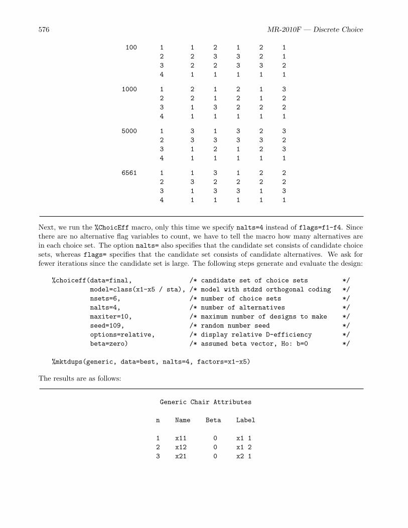
576 MR-2010F — Discrete Choice
100 1 1 2 1 2 12 2 3 3 2 13 2 2 3 3 24 1 1 1 1 1
1000 1 2 1 2 1 32 2 1 2 1 23 1 3 2 2 24 1 1 1 1 1
5000 1 3 1 3 2 32 3 3 3 3 23 1 2 1 2 34 1 1 1 1 1
6561 1 1 3 1 2 22 3 2 2 2 23 1 3 3 1 34 1 1 1 1 1
Next, we run the %ChoicEff macro, only this time we specify nalts=4 instead of flags=f1-f4. Sincethere are no alternative flag variables to count, we have to tell the macro how many alternatives arein each choice set. The option nalts= also specifies that the candidate set consists of candidate choicesets, whereas flags= specifies that the candidate set consists of candidate alternatives. We ask forfewer iterations since the candidate set is large. The following steps generate and evaluate the design:
%choiceff(data=final, /* candidate set of choice sets */model=class(x1-x5 / sta), /* model with stdzd orthogonal coding */nsets=6, /* number of choice sets */nalts=4, /* number of alternatives */maxiter=10, /* maximum number of designs to make */seed=109, /* random number seed */options=relative, /* display relative D-efficiency */beta=zero) /* assumed beta vector, Ho: b=0 */
%mktdups(generic, data=best, nalts=4, factors=x1-x5)
The results are as follows:
Generic Chair Attributes
n Name Beta Label
1 x11 0 x1 12 x12 0 x1 23 x21 0 x2 1

MR-2010F — Chair Design with Generic Attributes 577
4 x22 0 x2 25 x31 0 x3 16 x32 0 x3 27 x41 0 x4 18 x42 0 x4 29 x51 0 x5 110 x52 0 x5 2
Generic Chair Attributes
Design Iteration D-Efficiency D-Error----------------------------------------------
1 0 2.78600 * 0.358941 4.40738 * 0.226892 4.53259 * 0.220623 4.53259 0.22062
.
.
.
Design Iteration D-Efficiency D-Error----------------------------------------------
5 0 2.75184 0.363391 4.34618 0.230092 4.47415 0.223513 4.67101 * 0.214094 4.69946 * 0.212795 4.69946 0.21279
.
.
.
Design Iteration D-Efficiency D-Error----------------------------------------------
10 0 2.80475 0.356541 4.26387 0.234532 4.40048 0.227253 4.51659 0.221414 4.51659 0.22141

578 MR-2010F — Discrete Choice
Generic Chair Attributes
Final Results
Design 5Choice Sets 6Alternatives 4Parameters 10Maximum Parameters 18D-Efficiency 4.6995Relative D-Eff 78.3243D-Error 0.21281 / Choice Sets 0.1667
Generic Chair Attributes
Variable Standardn Name Label Variance DF Error
1 x11 x1 1 0.19102 1 0.437052 x12 x1 2 0.37907 1 0.615683 x21 x2 1 0.24790 1 0.497904 x22 x2 2 0.27501 1 0.524415 x31 x3 1 0.19389 1 0.440336 x32 x3 2 0.23730 1 0.487137 x41 x4 1 0.22452 1 0.473848 x42 x4 2 0.21910 1 0.468099 x51 x5 1 0.21234 1 0.4608110 x52 x5 2 0.24140 1 0.49133
==10
Design: GenericFactors: x1-x5
x1 x2 x3 x4 x5Sets w Dup Alts: 0Duplicate Sets: 0
This design is less D-efficient than we found using the alternative-swapping algorithm, so we will notuse it.

MR-2010F — Chair Design with Generic Attributes 579
Design Algorithm Comparisons
It is instructive to compare the three approaches outlined in this chapter in the context of this problem.There are 33×5 = 14, 348, 907 choice sets for this problem (three-level factors and 3 alternatives times 5factors per alternative). If we were to use the linear arrangement approach using the %MktEx macro, wecould never begin to consider all possible candidate choice sets. Similarly, with the choice-set-swappingalgorithm of the %ChoicEff macro, we could never begin to consider all possible candidate choice sets.Furthermore, with the linear arrangement approach, we could not create a design with six choice setssince the minimum size is 2 × 15 + 1 = 31. Now consider the alternative-swapping algorithm. It usesat most a candidate set with only 244 observations (35 + 1). From it, every possible choice set canpotentially be constructed, although the macro only considers a tiny fraction of the possibilities. Hence,alternative swapping usually finds a better design, because the candidate set does not limit it.
Both uses of the %ChoicEff macro have the advantage that they are explicitly minimizing the variancesof the parameter estimates given a model and a β vector. They can be used to produce smaller, morespecialized, and better designs. However, if the β vector or model is badly misspecified, the designscould be horrible. How badly do things have to be misspecified before you will have problems? Whoknows. More research is needed. In contrast, the linear model %MktEx approach is very conservativeand safe in that it should let you specify a very general model and still produce estimable parameters.The cost is you might be using many more choice sets than you need, particularly for nonbrandedgeneric attributes. If you really have some information about your parameters, you should use them toproduce a smaller and better design. However, if you have little or no information about parametersand if you anticipate specifying very general models like mother logit, then you probably want to usethe linear arrangement approach.

580 MR-2010F — Discrete Choice
Initial Designs
This section illustrates some design strategies that involve improving on or augmenting initial designs.We will not actually use any designs from this section.
Improving an Existing Design
Sometimes, it is useful to try to improve an existing design. In this example, we use the %MktEx macroto create a design in 80 runs for 25 four-level factors. In the next step, we specify init=, and themacro goes straight into the design refinement history seeking to refine the input design. You mightwant to do this, for example, whenever you have a good, but not 100% D-efficient design, and you arewilling to wait a few minutes to see if the macro can make it any better. The following steps generatethe design:
title ’Try to Improve an Existing Design’;
%mktex(4 ** 25, n=80, seed=368)
%mktex(4 ** 25, /* 25 four-level factors */n=80, /* number of runs */init=design, /* initial design */seed=306, /* random number seed */maxtime=20) /* maximum time in minutes to work */
The D-efficiency of the final design from the first step is as follows:
Try to Improve an Existing Design
The OPTEX Procedure
AveragePrediction
Design StandardNumber D-Efficiency A-Efficiency G-Efficiency Error------------------------------------------------------------------------
1 91.4106 83.9583 97.6073 0.9747
This is a large problem—one in which the maxtime= option might cause the macro to stop before itreaches the maximum number of iterations. Running a second refinement step might help improve thedesign by adding a few more iterations.

MR-2010F — Initial Designs 581
The results from the second step are as follows:
Design Refinement History
Current BestDesign Row,Col D-Efficiency D-Efficiency Notes----------------------------------------------------------
0 Initial 91.4106 91.4106 Ini
1 Start 90.0771 Pre,Mut,Ann1 End 91.3476
2 Start 88.8927 Pre,Mut,Ann2 36 12 91.4181 91.41812 56 6 91.4285 91.42852 7 17 91.4372 91.43722 13 10 91.4373 91.43732 23 18 91.4404 91.44042 17 16 91.4445 91.44452 34 6 91.4572 91.45722 56 19 91.4673 91.46732 56 21 91.4768 91.47682 77 1 91.4821 91.48212 23 18 91.4827 91.48272 48 3 91.4848 91.48482 48 9 91.4863 91.48632 40 18 91.4863 91.48632 End 91.4863
.
.
.
6 Start 90.2194 Pre,Mut,Ann6 63 19 91.5811 91.58116 68 18 91.5835 91.58356 End 91.5751

582 MR-2010F — Discrete Choice
7 Start 89.4607 Pre,Mut,Ann7 25 4 91.5851 91.58517 34 7 91.5902 91.59027 47 2 91.5913 91.59137 48 14 91.5930 91.59307 56 4 91.5955 91.59557 56 15 91.5999 91.59997 60 6 91.6142 91.61427 68 7 91.6172 91.61727 78 5 91.6172 91.61727 13 21 91.6249 91.62497 18 19 91.6249 91.62497 43 10 91.6249 91.62497 48 14 91.6282 91.62827 50 22 91.6408 91.64087 61 4 91.6417 91.64177 80 15 91.6430 91.64307 46 12 91.6430 91.64307 48 6 91.6430 91.64307 End 91.6430
.
.
.
10 Start 89.8707 Pre,Mut,Ann10 End 91.6629
.
.
.
Try to Improve an Existing Design
The OPTEX Procedure
AveragePrediction
Design StandardNumber D-Efficiency A-Efficiency G-Efficiency Error------------------------------------------------------------------------
1 91.7082 83.9853 97.5951 0.9747
The macro skips the normal first steps, algorithm search and design search, and goes straight intothe design refinement search. In this example a small improvement is found, although often, noimprovement is found.

MR-2010F — Initial Designs 583
When Some Choice Sets are Fixed in Advance
Sometimes certain runs or choice sets are fixed in advance and must be included in the design. The%MktEx macro can be used to efficiently augment a starting design with other choice sets. Suppose thatyou can make a choice design from the L36 (211312). In addition, you want to optimally add four morechoice sets to use as holdouts. First we look at how to do this using the fixed= option. This optioncan be used for fairly general design augmentation and refinement problems. On page 587, we see aneasier way to handle this particular problem using the holdouts= option.
You can create the design in 36 runs as before. Next, a DATA step is used to add a flag variable f thathas values of 1 for the original 36 runs. In addition, four more runs are added (just copies of the lastrun) but with a flag value of missing. When this variable is specified in the fixed=f option, it indicatesthat the first 36 runs of the init=init design are fixed—they must not change. The remaining 4 runsare to be randomly initialized and optimally refined to maximize the D-efficiency of the overall 40-rundesign. We specify options=nosort so that the additional runs stay at the end of the design. Thefollowing steps generate and display the design:
title ’Augment a Design’;
%mktex(n=36, seed=292)
data init;set randomized end = eof;f = 1;output;
if eof then do;f = .;do i = 1 to 4; output; end;drop i;end;
run;
proc print; run;
%mktex(2 ** 11 3 ** 12, /* 11 2-level and 12 3-level factors */n=40, /* 40 runs in final design */init=init, /* initial design */fixed=f, /* f var flags runs that cannot change */seed=513, /* random number seed */options=nosort) /* do not sort output design */
proc print; run;
The initial design is as follows:

584 MR-2010F — Discrete Choice
Augment a Design
O x x x x x x x x x x x x x xb x x x x x x x x x 1 1 1 1 1 1 1 1 1 1 2 2 2 2s 1 2 3 4 5 6 7 8 9 0 1 2 3 4 5 6 7 8 9 0 1 2 3 f
1 2 1 2 2 2 2 1 1 1 2 1 2 3 1 1 1 2 3 2 3 1 3 2 12 2 1 1 2 2 1 2 1 2 1 2 3 1 2 1 3 2 3 1 2 2 3 1 13 2 2 1 1 1 1 1 1 1 2 2 1 2 3 1 1 2 2 3 2 3 3 3 14 1 1 1 1 2 1 1 2 2 2 1 1 2 3 2 3 2 3 2 1 2 1 2 15 1 2 1 2 2 2 1 2 1 1 2 1 1 2 2 2 1 3 3 3 3 3 2 16 2 1 1 2 2 1 2 1 2 1 2 1 2 1 3 2 1 2 2 3 1 1 3 17 1 2 2 1 2 1 2 1 1 1 1 3 3 2 2 1 1 2 2 1 2 3 3 18 2 2 1 1 1 1 1 1 1 2 2 2 3 2 3 3 1 1 1 3 2 1 2 19 2 2 2 2 1 1 1 2 2 1 1 2 2 2 3 3 3 3 3 1 1 3 3 110 2 2 2 2 1 1 1 2 2 1 1 1 1 3 1 1 1 1 2 3 2 2 1 111 1 1 2 1 1 2 1 1 2 1 2 3 2 2 2 1 2 1 3 3 1 1 1 112 2 2 2 1 2 2 2 2 2 2 2 1 3 3 2 3 3 2 1 3 1 3 1 113 1 2 1 2 2 2 1 2 1 1 2 3 3 3 3 3 2 1 2 2 1 2 3 114 1 1 2 1 1 2 1 1 2 1 2 1 3 1 1 3 1 3 1 1 3 2 3 115 2 1 1 1 1 2 2 2 1 1 1 1 3 2 3 1 3 3 2 2 3 1 1 116 1 2 2 1 2 1 2 1 1 1 1 2 2 3 3 2 2 3 1 3 3 2 1 117 2 1 1 1 1 2 2 2 1 1 1 3 2 3 1 2 1 1 1 1 1 3 2 118 1 1 1 1 2 1 1 2 2 2 1 3 1 1 3 1 3 1 1 3 3 3 3 119 2 1 2 2 2 2 1 1 1 2 1 1 2 2 2 2 3 1 1 2 2 2 3 120 2 1 1 1 1 2 2 2 1 1 1 2 1 1 2 3 2 2 3 3 2 2 3 121 1 2 1 2 1 2 2 1 2 2 1 1 3 1 3 2 2 1 3 1 2 3 1 122 1 1 2 1 1 2 1 1 2 1 2 2 1 3 3 2 3 2 2 2 2 3 2 123 2 2 2 1 2 2 2 2 2 2 2 3 2 1 3 1 1 3 3 2 2 2 2 124 1 2 2 1 2 1 2 1 1 1 1 1 1 1 1 3 3 1 3 2 1 1 2 125 1 1 2 2 1 1 2 2 1 2 2 1 1 2 3 1 2 2 1 1 1 2 2 126 1 1 2 2 1 1 2 2 1 2 2 2 2 1 2 3 1 1 2 2 3 3 1 127 1 1 2 2 1 1 2 2 1 2 2 3 3 3 1 2 3 3 3 3 2 1 3 128 1 2 1 2 2 2 1 2 1 1 2 2 2 1 1 1 3 2 1 1 2 1 1 129 2 1 2 2 2 2 1 1 1 2 1 3 1 3 3 3 1 2 3 1 3 1 1 130 2 2 1 1 1 1 1 1 1 2 2 3 1 1 2 2 3 3 2 1 1 2 1 131 1 2 1 2 1 2 2 1 2 2 1 2 1 3 2 1 1 3 1 2 1 1 3 132 2 1 1 2 2 1 2 1 2 1 2 2 3 3 2 1 3 1 3 1 3 2 2 133 2 2 2 2 1 1 1 2 2 1 1 3 3 1 2 2 2 2 1 2 3 1 2 134 1 2 1 2 1 2 2 1 2 2 1 3 2 2 1 3 3 2 2 3 3 2 2 135 2 2 2 1 2 2 2 2 2 2 2 2 1 2 1 2 2 1 2 1 3 1 3 136 1 1 1 1 2 1 1 2 2 2 1 2 3 2 1 2 1 2 3 2 1 2 1 137 1 1 1 1 2 1 1 2 2 2 1 2 3 2 1 2 1 2 3 2 1 2 1 .38 1 1 1 1 2 1 1 2 2 2 1 2 3 2 1 2 1 2 3 2 1 2 1 .39 1 1 1 1 2 1 1 2 2 2 1 2 3 2 1 2 1 2 3 2 1 2 1 .40 1 1 1 1 2 1 1 2 2 2 1 2 3 2 1 2 1 2 3 2 1 2 1 .

MR-2010F — Initial Designs 585
The iteration history for the augmentation is as follows:
Augment a Design
Design Refinement History
Current BestDesign Row,Col D-Efficiency D-Efficiency Notes----------------------------------------------------------
0 Initial 97.0559 97.0559 Ini
1 Start 97.0788 97.0788 Pre,Mut,Ann1 37 5 97.0805 97.08051 37 8 97.0816 97.08161 37 9 97.1049 97.10491 37 11 97.1133 97.11331 37 13 97.1177 97.11771 38 1 97.1410 97.14101 38 2 97.1605 97.16051 38 3 97.1729 97.17291 38 4 97.1822 97.18221 38 6 97.1905 97.19051 38 8 97.1944 97.19441 39 2 97.1991 97.19911 39 13 97.2007 97.20071 39 19 97.2007 97.20071 40 9 97.2007 97.20071 40 10 97.2007 97.20071 37 18 97.2023 97.20231 37 3 97.2028 97.20281 37 4 97.2028 97.20281 37 23 97.2043 97.20431 End 97.2043
2 Start 97.2043 97.2043 Pre,Mut,Ann2 40 21 97.2043 97.20432 38 2 97.2043 97.20432 40 9 97.2043 97.20432 40 21 97.2043 97.20432 End 97.2043
3 Start 97.2043 97.2043 Pre,Mut,Ann3 End 97.2043
4 Start 97.2002 Pre,Mut,Ann4 39 12 97.2043 97.20434 39 23 97.2043 97.20434 39 16 97.2043 97.20434 End 97.2043

586 MR-2010F — Discrete Choice
5 Start 97.2043 97.2043 Pre,Mut,Ann5 37 3 97.2043 97.20435 37 15 97.2043 97.20435 End 97.2043
6 Start 97.2043 97.2043 Pre,Mut,Ann6 40 1 97.2043 97.20436 39 16 97.2043 97.20436 38 16 97.2043 97.20436 End 97.2043
NOTE: Stopping since it appears that no improvement is possible.
Notice that the macro goes straight into the design refinement stage. Also notice that in the iterationhistory, only rows 37 through 40 are changed. The design is as follows:
Augment a Design
O x x x x x x x x x x x x x xb x x x x x x x x x 1 1 1 1 1 1 1 1 1 1 2 2 2 2s 1 2 3 4 5 6 7 8 9 0 1 2 3 4 5 6 7 8 9 0 1 2 3 f
1 2 1 2 2 2 2 1 1 1 2 1 2 3 1 1 1 2 3 2 3 1 3 2 12 2 1 1 2 2 1 2 1 2 1 2 3 1 2 1 3 2 3 1 2 2 3 1 13 2 2 1 1 1 1 1 1 1 2 2 1 2 3 1 1 2 2 3 2 3 3 3 14 1 1 1 1 2 1 1 2 2 2 1 1 2 3 2 3 2 3 2 1 2 1 2 15 1 2 1 2 2 2 1 2 1 1 2 1 1 2 2 2 1 3 3 3 3 3 2 16 2 1 1 2 2 1 2 1 2 1 2 1 2 1 3 2 1 2 2 3 1 1 3 17 1 2 2 1 2 1 2 1 1 1 1 3 3 2 2 1 1 2 2 1 2 3 3 18 2 2 1 1 1 1 1 1 1 2 2 2 3 2 3 3 1 1 1 3 2 1 2 19 2 2 2 2 1 1 1 2 2 1 1 2 2 2 3 3 3 3 3 1 1 3 3 110 2 2 2 2 1 1 1 2 2 1 1 1 1 3 1 1 1 1 2 3 2 2 1 111 1 1 2 1 1 2 1 1 2 1 2 3 2 2 2 1 2 1 3 3 1 1 1 112 2 2 2 1 2 2 2 2 2 2 2 1 3 3 2 3 3 2 1 3 1 3 1 113 1 2 1 2 2 2 1 2 1 1 2 3 3 3 3 3 2 1 2 2 1 2 3 114 1 1 2 1 1 2 1 1 2 1 2 1 3 1 1 3 1 3 1 1 3 2 3 115 2 1 1 1 1 2 2 2 1 1 1 1 3 2 3 1 3 3 2 2 3 1 1 116 1 2 2 1 2 1 2 1 1 1 1 2 2 3 3 2 2 3 1 3 3 2 1 117 2 1 1 1 1 2 2 2 1 1 1 3 2 3 1 2 1 1 1 1 1 3 2 118 1 1 1 1 2 1 1 2 2 2 1 3 1 1 3 1 3 1 1 3 3 3 3 119 2 1 2 2 2 2 1 1 1 2 1 1 2 2 2 2 3 1 1 2 2 2 3 120 2 1 1 1 1 2 2 2 1 1 1 2 1 1 2 3 2 2 3 3 2 2 3 1

MR-2010F — Initial Designs 587
21 1 2 1 2 1 2 2 1 2 2 1 1 3 1 3 2 2 1 3 1 2 3 1 122 1 1 2 1 1 2 1 1 2 1 2 2 1 3 3 2 3 2 2 2 2 3 2 123 2 2 2 1 2 2 2 2 2 2 2 3 2 1 3 1 1 3 3 2 2 2 2 124 1 2 2 1 2 1 2 1 1 1 1 1 1 1 1 3 3 1 3 2 1 1 2 125 1 1 2 2 1 1 2 2 1 2 2 1 1 2 3 1 2 2 1 1 1 2 2 126 1 1 2 2 1 1 2 2 1 2 2 2 2 1 2 3 1 1 2 2 3 3 1 127 1 1 2 2 1 1 2 2 1 2 2 3 3 3 1 2 3 3 3 3 2 1 3 128 1 2 1 2 2 2 1 2 1 1 2 2 2 1 1 1 3 2 1 1 2 1 1 129 2 1 2 2 2 2 1 1 1 2 1 3 1 3 3 3 1 2 3 1 3 1 1 130 2 2 1 1 1 1 1 1 1 2 2 3 1 1 2 2 3 3 2 1 1 2 1 131 1 2 1 2 1 2 2 1 2 2 1 2 1 3 2 1 1 3 1 2 1 1 3 132 2 1 1 2 2 1 2 1 2 1 2 2 3 3 2 1 3 1 3 1 3 2 2 133 2 2 2 2 1 1 1 2 2 1 1 3 3 1 2 2 2 2 1 2 3 1 2 134 1 2 1 2 1 2 2 1 2 2 1 3 2 2 1 3 3 2 2 3 3 2 2 135 2 2 2 1 2 2 2 2 2 2 2 2 1 2 1 2 2 1 2 1 3 1 3 136 1 1 1 1 2 1 1 2 2 2 1 2 3 2 1 2 1 2 3 2 1 2 1 137 1 2 2 2 2 1 1 2 1 1 1 3 2 3 3 2 1 2 1 3 1 3 1 .38 2 2 2 1 2 1 2 2 1 1 1 2 2 1 2 3 3 3 1 1 3 2 3 .39 1 2 2 2 2 2 2 1 2 2 2 3 3 3 1 2 1 3 2 1 3 2 3 .40 2 1 1 1 1 1 1 2 2 2 1 2 1 2 3 2 1 3 2 1 1 2 1 .
The last four rows are the holdouts.
The following steps do the same thing only using the holdouts=4 option instead:
title ’Augment a Design’;
%mktex(n=36, seed=292)
%mktex(2 ** 11 3 ** 12, /* 11 2-level and 12 3-level factors */n=40, /* 40 runs in final design */init=randomized, /* initial design with 36 runs */holdouts=4, /* add four holdouts */seed=513, /* random number seed */options=nosort) /* do not sort output design */
proc print data=design(firstobs=37); run;
The holdout observations, which are the same as we saw previously, are as follows:

588 MR-2010F — Discrete Choice
Augment a Design
O x x x x x x x x x x x x x xb x x x x x x x x x 1 1 1 1 1 1 1 1 1 1 2 2 2 2s 1 2 3 4 5 6 7 8 9 0 1 2 3 4 5 6 7 8 9 0 1 2 3 w
37 1 2 2 2 2 1 1 2 1 1 1 3 2 3 3 2 1 2 1 3 1 3 1 .38 2 2 2 1 2 1 2 2 1 1 1 2 2 1 2 3 3 3 1 1 3 2 3 .39 1 2 2 2 2 2 2 1 2 2 2 3 3 3 1 2 1 3 2 1 3 2 3 .40 2 1 1 1 1 1 1 2 2 2 1 2 1 2 3 2 1 3 2 1 1 2 1 .
The %MktEx macro provides another way to use initial designs. The initial design can indicate thatpart of the design is fixed and cannot change and a different part should be randomly initialized andcan change. The initial design can have three types of values:
• positive integers are fixed and constant and do not change throughout the course of the iterations.
• zero and missing values are replaced by random values at the start of each new design search andcan change throughout the course of the iterations.
• negative values are replaced by their absolute value at the start of each new design attempt andcan change throughout the course of the iterations.
Returning to the example of making the design 425 in 80 runs, we could do it in two steps. The maximumnumber of four-level factors in 80 runs is 11. If it is important that some factors be orthogonal, wecould first make an orthogonal array with 11 four-level factors and then append 14 more nonorthogonal-factors. The following steps create the design:
title ’Differential Design Initialization’;
%mktex(4 ** 11, n=80)
data init;set design;retain x12-x25 .;run;
%mktex(4 ** 25, /* 25 four-level factors */n=80, /* 80 runs */init=init, /* initial design */seed=472) /* random number seed */
%mkteval;
The initial design consists of the orthogonal array with 11 columns followed by 14 more columns thatare all missing. When %MktEx sees missing values in the initial design, it holds all the nonmissingvalues fixed. Then it randomly replaces the missing values and uses the coordinate-exchange algorithmto refine the last columns. The final design is slightly less D-efficient than we saw previously, but the

MR-2010F — Initial Designs 589
first 11 columns are orthogonal. The remaining columns are all slightly correlated with themselves andwith the first columns. The final efficiency table is as follows:
Differential Design Initialization
AveragePrediction
Design StandardNumber D-Efficiency A-Efficiency G-Efficiency Error------------------------------------------------------------------------
1 89.4216 78.9807 97.7767 0.9747
The canonical correlations are as follows:
Differential Design InitializationCanonical Correlations Between the Factors
There are 0 Canonical Correlations Greater Than 0.316
x1 x2 x3 x4 x5 x6 x7 x8 x9 x10 x11 x12 x13
x1 1 0 0 0 0 0 0 0 0 0 0 0.15 0.17x2 0 1 0 0 0 0 0 0 0 0 0 0.17 0.11x3 0 0 1 0 0 0 0 0 0 0 0 0.20 0.13x4 0 0 0 1 0 0 0 0 0 0 0 0.16 0.12x5 0 0 0 0 1 0 0 0 0 0 0 0.16 0.18x6 0 0 0 0 0 1 0 0 0 0 0 0.12 0.12x7 0 0 0 0 0 0 1 0 0 0 0 0.18 0.18x8 0 0 0 0 0 0 0 1 0 0 0 0.16 0.12x9 0 0 0 0 0 0 0 0 1 0 0 0.15 0.14x10 0 0 0 0 0 0 0 0 0 1 0 0.12 0.18x11 0 0 0 0 0 0 0 0 0 0 1 0.16 0.12x12 0.15 0.17 0.20 0.16 0.16 0.12 0.18 0.16 0.15 0.12 0.16 1 0.10x13 0.17 0.11 0.13 0.12 0.18 0.12 0.18 0.12 0.14 0.18 0.12 0.10 1x14 0.18 0.14 0.10 0.14 0.19 0.20 0.18 0.19 0.14 0.15 0.11 0.16 0.15x15 0.16 0.25 0.15 0.18 0.17 0.17 0.15 0.12 0.24 0.13 0.16 0.14 0.13x16 0.10 0.23 0.14 0.15 0.17 0.16 0.15 0.13 0.10 0.16 0.21 0.12 0.11x17 0.20 0.20 0.15 0.07 0.12 0.17 0.16 0.12 0.13 0.20 0.14 0.12 0.11x18 0.09 0.18 0.10 0.16 0.15 0.13 0.13 0.17 0.10 0.15 0.14 0.15 0.09x19 0.17 0.18 0.17 0.16 0.13 0.17 0.19 0.21 0.15 0.15 0.16 0.14 0.15x20 0.23 0.09 0.11 0.14 0.17 0.21 0.25 0.27 0.06 0.17 0.15 0.14 0.11x21 0.12 0.09 0.15 0.17 0.17 0.15 0.20 0.14 0.20 0.17 0.16 0.18 0.12x22 0.17 0.14 0.07 0.18 0.15 0.12 0.11 0.16 0.17 0.09 0.17 0.12 0.16x23 0.19 0.15 0.15 0.18 0.09 0.10 0.16 0.16 0.12 0.16 0.16 0.13 0.12x24 0.18 0.16 0.14 0.20 0.09 0.22 0.13 0.13 0.18 0.13 0.18 0.14 0.11x25 0.14 0.18 0.09 0.13 0.19 0.18 0.17 0.19 0.16 0.20 0.14 0.15 0.12

590 MR-2010F — Discrete Choice
x14 x15 x16 x17 x18 x19 x20 x21 x22 x23 x24 x25
x1 0.18 0.16 0.10 0.20 0.09 0.17 0.23 0.12 0.17 0.19 0.18 0.14x2 0.14 0.25 0.23 0.20 0.18 0.18 0.09 0.09 0.14 0.15 0.16 0.18x3 0.10 0.15 0.14 0.15 0.10 0.17 0.11 0.15 0.07 0.15 0.14 0.09x4 0.14 0.18 0.15 0.07 0.16 0.16 0.14 0.17 0.18 0.18 0.20 0.13x5 0.19 0.17 0.17 0.12 0.15 0.13 0.17 0.17 0.15 0.09 0.09 0.19x6 0.20 0.17 0.16 0.17 0.13 0.17 0.21 0.15 0.12 0.10 0.22 0.18x7 0.18 0.15 0.15 0.16 0.13 0.19 0.25 0.20 0.11 0.16 0.13 0.17x8 0.19 0.12 0.13 0.12 0.17 0.21 0.27 0.14 0.16 0.16 0.13 0.19x9 0.14 0.24 0.10 0.13 0.10 0.15 0.06 0.20 0.17 0.12 0.18 0.16x10 0.15 0.13 0.16 0.20 0.15 0.15 0.17 0.17 0.09 0.16 0.13 0.20x11 0.11 0.16 0.21 0.14 0.14 0.16 0.15 0.16 0.17 0.16 0.18 0.14x12 0.16 0.14 0.12 0.12 0.15 0.14 0.14 0.18 0.12 0.13 0.14 0.15x13 0.15 0.13 0.11 0.11 0.09 0.15 0.11 0.12 0.16 0.12 0.11 0.12x14 1 0.22 0.14 0.12 0.12 0.21 0.13 0.13 0.13 0.20 0.18 0.12x15 0.22 1 0.12 0.09 0.19 0.09 0.09 0.13 0.10 0.15 0.16 0.13x16 0.14 0.12 1 0.15 0.14 0.14 0.18 0.13 0.12 0.10 0.17 0.18x17 0.12 0.09 0.15 1 0.09 0.16 0.18 0.09 0.15 0.12 0.18 0.12x18 0.12 0.19 0.14 0.09 1 0.14 0.13 0.20 0.15 0.13 0.14 0.17x19 0.21 0.09 0.14 0.16 0.14 1 0.13 0.11 0.10 0.11 0.16 0.12x20 0.13 0.09 0.18 0.18 0.13 0.13 1 0.10 0.11 0.11 0.18 0.11x21 0.13 0.13 0.13 0.09 0.20 0.11 0.10 1 0.21 0.15 0.23 0.09x22 0.13 0.10 0.12 0.15 0.15 0.10 0.11 0.21 1 0.19 0.18 0.22x23 0.20 0.15 0.10 0.12 0.13 0.11 0.11 0.15 0.19 1 0.13 0.13x24 0.18 0.16 0.17 0.18 0.14 0.16 0.18 0.23 0.18 0.13 1 0.12x25 0.12 0.13 0.18 0.12 0.17 0.12 0.11 0.09 0.22 0.13 0.12 1
The one-way frequencies are as follows:
Differential Design InitializationSummary of Frequencies
There are 0 Canonical Correlations Greater Than 0.316* - Indicates Unequal Frequencies
Frequencies
x1 20 20 20 20x2 20 20 20 20x3 20 20 20 20x4 20 20 20 20x5 20 20 20 20x6 20 20 20 20x7 20 20 20 20x8 20 20 20 20x9 20 20 20 20x10 20 20 20 20x11 20 20 20 20

MR-2010F — Initial Designs 591
* x12 19 22 19 20* x13 21 19 20 20* x14 18 20 21 21* x15 18 21 22 19* x16 19 18 22 21* x17 21 19 18 22* x18 21 20 20 19* x19 21 18 18 23* x20 20 20 21 19* x21 18 20 23 19* x22 20 18 22 20* x23 19 20 21 20* x24 23 17 20 20* x25 21 19 19 21
We could run one more refinement on this design and force x12-x25 to be balanced. We need to makea new initial design using our current design. This time, we make x12-x25 negative. Then x1-x11 donot change, the absolute values of x12-x25 are used as initial values, but x12-x25 are still be allowed tochange. Then we can use the balance=1 option with %MktEx to make a design that is better balanced.Usually, when you are creating a design, you should specify mintry= with balance=, however, sincewe are refining not creating a design it is not necessary. The following steps create the design:
data init(drop=j);set design;array x[25];do j = 12 to 25; x[j] = -x[j]; end;run;
%mktex(4 ** 25, /* 25 four-level factors */n=80, /* 80 runs */init=init, /* initial design */seed=472, /* random number seed */balance=1) /* require near perfect balance */
%mkteval;
The final D-efficiency, which again, is a bit lower than we saw previously, is as follows:
Differential Design Initialization
AveragePrediction
Design StandardNumber D-Efficiency A-Efficiency G-Efficiency Error------------------------------------------------------------------------
1 86.1917 71.1301 97.9379 0.9747

592 MR-2010F — Discrete Choice
The canonical correlations are as follows:
Differential Design InitializationCanonical Correlations Between the Factors
There are 0 Canonical Correlations Greater Than 0.316
x1 x2 x3 x4 x5 x6 x7 x8 x9 x10 x11 x12 x13
x1 1 0 0 0 0 0 0 0 0 0 0 0.20 0.15x2 0 1 0 0 0 0 0 0 0 0 0 0.15 0.13x3 0 0 1 0 0 0 0 0 0 0 0 0.15 0.12x4 0 0 0 1 0 0 0 0 0 0 0 0.20 0.15x5 0 0 0 0 1 0 0 0 0 0 0 0.20 0.24x6 0 0 0 0 0 1 0 0 0 0 0 0.13 0.15x7 0 0 0 0 0 0 1 0 0 0 0 0.17 0.19x8 0 0 0 0 0 0 0 1 0 0 0 0.13 0.15x9 0 0 0 0 0 0 0 0 1 0 0 0.12 0.16x10 0 0 0 0 0 0 0 0 0 1 0 0.13 0.17x11 0 0 0 0 0 0 0 0 0 0 1 0.20 0.13x12 0.20 0.15 0.15 0.20 0.20 0.13 0.17 0.13 0.12 0.13 0.20 1 0.14x13 0.15 0.13 0.12 0.15 0.24 0.15 0.19 0.15 0.16 0.17 0.13 0.14 1x14 0.20 0.10 0.09 0.13 0.18 0.22 0.17 0.16 0.13 0.16 0.09 0.20 0.15x15 0.21 0.23 0.22 0.25 0.20 0.24 0.17 0.15 0.22 0.13 0.22 0.18 0.16x16 0.09 0.20 0.17 0.18 0.12 0.18 0.17 0.17 0.10 0.16 0.20 0.09 0.14x17 0.20 0.23 0.15 0.15 0.09 0.22 0.20 0.10 0.15 0.17 0.15 0.15 0.15x18 0.10 0.23 0.10 0.16 0.15 0.15 0.18 0.17 0.10 0.15 0.15 0.15 0.12x19 0.17 0.20 0.18 0.14 0.17 0.15 0.23 0.16 0.12 0.19 0.17 0.16 0.25x20 0.26 0.10 0.10 0.17 0.17 0.17 0.24 0.23 0.09 0.17 0.19 0.12 0.10x21 0.20 0.13 0.20 0.19 0.19 0.19 0.20 0.20 0.15 0.14 0.17 0.14 0.14x22 0.17 0.16 0.10 0.23 0.14 0.16 0.10 0.16 0.15 0.10 0.14 0.15 0.15x23 0.24 0.18 0.14 0.18 0.09 0.10 0.15 0.20 0.13 0.22 0.19 0.19 0.12x24 0.24 0.20 0.27 0.18 0.15 0.29 0.12 0.12 0.18 0.20 0.17 0.20 0.14x25 0.20 0.16 0.09 0.15 0.23 0.19 0.17 0.18 0.17 0.22 0.15 0.16 0.12
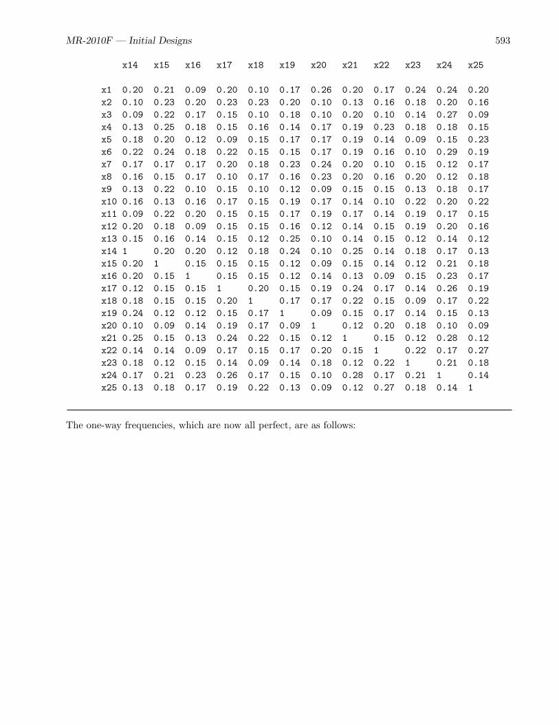
MR-2010F — Initial Designs 593
x14 x15 x16 x17 x18 x19 x20 x21 x22 x23 x24 x25
x1 0.20 0.21 0.09 0.20 0.10 0.17 0.26 0.20 0.17 0.24 0.24 0.20x2 0.10 0.23 0.20 0.23 0.23 0.20 0.10 0.13 0.16 0.18 0.20 0.16x3 0.09 0.22 0.17 0.15 0.10 0.18 0.10 0.20 0.10 0.14 0.27 0.09x4 0.13 0.25 0.18 0.15 0.16 0.14 0.17 0.19 0.23 0.18 0.18 0.15x5 0.18 0.20 0.12 0.09 0.15 0.17 0.17 0.19 0.14 0.09 0.15 0.23x6 0.22 0.24 0.18 0.22 0.15 0.15 0.17 0.19 0.16 0.10 0.29 0.19x7 0.17 0.17 0.17 0.20 0.18 0.23 0.24 0.20 0.10 0.15 0.12 0.17x8 0.16 0.15 0.17 0.10 0.17 0.16 0.23 0.20 0.16 0.20 0.12 0.18x9 0.13 0.22 0.10 0.15 0.10 0.12 0.09 0.15 0.15 0.13 0.18 0.17x10 0.16 0.13 0.16 0.17 0.15 0.19 0.17 0.14 0.10 0.22 0.20 0.22x11 0.09 0.22 0.20 0.15 0.15 0.17 0.19 0.17 0.14 0.19 0.17 0.15x12 0.20 0.18 0.09 0.15 0.15 0.16 0.12 0.14 0.15 0.19 0.20 0.16x13 0.15 0.16 0.14 0.15 0.12 0.25 0.10 0.14 0.15 0.12 0.14 0.12x14 1 0.20 0.20 0.12 0.18 0.24 0.10 0.25 0.14 0.18 0.17 0.13x15 0.20 1 0.15 0.15 0.15 0.12 0.09 0.15 0.14 0.12 0.21 0.18x16 0.20 0.15 1 0.15 0.15 0.12 0.14 0.13 0.09 0.15 0.23 0.17x17 0.12 0.15 0.15 1 0.20 0.15 0.19 0.24 0.17 0.14 0.26 0.19x18 0.18 0.15 0.15 0.20 1 0.17 0.17 0.22 0.15 0.09 0.17 0.22x19 0.24 0.12 0.12 0.15 0.17 1 0.09 0.15 0.17 0.14 0.15 0.13x20 0.10 0.09 0.14 0.19 0.17 0.09 1 0.12 0.20 0.18 0.10 0.09x21 0.25 0.15 0.13 0.24 0.22 0.15 0.12 1 0.15 0.12 0.28 0.12x22 0.14 0.14 0.09 0.17 0.15 0.17 0.20 0.15 1 0.22 0.17 0.27x23 0.18 0.12 0.15 0.14 0.09 0.14 0.18 0.12 0.22 1 0.21 0.18x24 0.17 0.21 0.23 0.26 0.17 0.15 0.10 0.28 0.17 0.21 1 0.14x25 0.13 0.18 0.17 0.19 0.22 0.13 0.09 0.12 0.27 0.18 0.14 1
The one-way frequencies, which are now all perfect, are as follows:

594 MR-2010F — Discrete Choice
Differential Design Initialization
Summary of FrequenciesThere are 0 Canonical Correlations Greater Than 0.316
* - Indicates Unequal Frequencies
Frequencies
x1 20 20 20 20x2 20 20 20 20x3 20 20 20 20x4 20 20 20 20x5 20 20 20 20x6 20 20 20 20x7 20 20 20 20x8 20 20 20 20x9 20 20 20 20x10 20 20 20 20x11 20 20 20 20x12 20 20 20 20x13 20 20 20 20x14 20 20 20 20x15 20 20 20 20x16 20 20 20 20x17 20 20 20 20x18 20 20 20 20x19 20 20 20 20x20 20 20 20 20x21 20 20 20 20x22 20 20 20 20x23 20 20 20 20x24 20 20 20 20x25 20 20 20 20
You can initialize any part of the design to positive integers (fixed), any other part to zero or missing(randomly initialize and change), and any other part to negative (do not reinitialize but change isallowed). This capability gives you very flexible control over the components of your design.

MR-2010F — Partial Profiles and Restrictions 595
Partial Profiles and Restrictions
Partial-profile designs (Chrzan and Elrod 1995) are used when there are many attributes but no morethan a few of them are allowed to vary at any one time. Chrzan and Elrod show an example whererespondents must choose between vacuum cleaners that vary along 20 different attributes: Brand,Price, Warranty, Horsepower, and so on. It is difficult for respondents to simultaneously evaluate thatmany attributes, so it is better if they are only exposed to a few at a time. Partial-profile designs havebecome very popular among some researchers.
This section serves two purposes. It shows ways in which partial-profile designs can be made. It alsoillustrates some of the important techniques available for restricting designs with the %MktEx macro.Partial-profile designs provide a nice context for illustrating the creation of highly-restricted designs.
Pairwise Partial-Profile Choice Design
For example, a partial-profile design for 20 two-level factors, with 5 varying at a time, with the factorsthat are not shown displayed with an ordinary missing value is as follows:
. . . 2 . . . 1 1 1 . . . . 1 . . . . .2 . . . 2 . . . . . 1 . . . . . 1 . . 12 . 1 . . . . 1 . . . . . 1 . . . . . 2. . . . . . . 2 . . . . . 2 2 . . 2 2 .. . . . 2 . . . . 2 . 2 . . . 2 . 2 . .. . . . . . . . 2 . . . . 1 . . . 2 1 1. . . . . . . . 1 . 2 . 2 . . . 2 . . 21 . . . . 1 . . . . . . . 2 . 2 . . . 1. . . . . . 2 . . . . 2 1 . 2 . . . . 1. . 1 . 1 . . . . 2 . . . . . 1 . . . 11 . 2 . . . 2 . . . . . . . . . 1 2 . .. 1 . . . . . . . . 2 . 1 . 1 1 . . . .2 . . . . . . . 2 . . 2 . . . 1 2 . . .. . 1 . . . . . . . . 2 2 . 1 . . . 1 .. . . . 2 . 2 . . . . . . 2 . 1 . . 1 .. 2 . 1 . . . 1 . . . . . . . . 2 . 2 .2 2 . . . . 1 . 1 . . 1 . . . . . . . .. 2 . . . . . . . 1 1 . . . . . . 1 . 2. 1 . 1 . 2 . 2 . . . . . . . . . 1 . .. . . 1 1 . . . . . 2 2 . 1 . . . . . .1 . . . 2 2 1 . . . . . . . 2 . . . . .. . . . . 1 1 2 . 1 . . . . . . 1 . . .. . . 2 . . . . . . . 1 2 1 . 1 . . . .. . . 1 . . . . 2 . . 1 . . 1 . . . . 2. . 2 . . 1 . . 1 . 1 . . . 2 . . . . .. . 2 . 1 . . 2 . . . . 1 . . 2 . . . .. . 2 . . . 1 1 . . 2 . . . . . . 1 . .. 1 . . 1 . . 1 2 . . . 2 . . . . . . .1 . . . . . . . 1 . . . 1 . . . . 1 2 .2 . . 2 1 1 . . . . . . . . . . . 2 . .
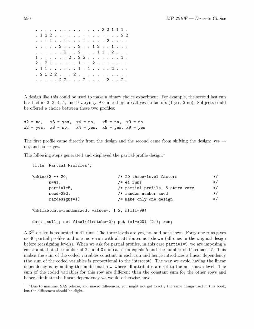
596 MR-2010F — Discrete Choice
. . . . . . . . . . . . . . 2 2 1 1 1 .
. 1 2 2 . . . . . . . . . . . . . . 2 2
. . 1 1 . . 1 . . . 1 . . . . 2 . . . .
. . . . . 2 . . . 2 . . 1 2 . . 1 . . .
. . . . . . 2 . . 2 . . . 1 1 . 2 . . .1 . . . . . . 2 . 2 2 . . . . . . . 1 .2 . 2 1 . . . . . 1 . . 2 . . . . . . .. 1 1 . . . . . . 1 . 1 . . . . 2 . . .. 2 1 2 2 . . . 2 . . . . . . . . . . .. . . . . 2 2 . . . 2 . . . . 2 . . 2 .
A design like this could be used to make a binary choice experiment. For example, the second last runhas factors 2, 3, 4, 5, and 9 varying. Assume they are all yes-no factors (1 yes, 2 no). Subjects couldbe offered a choice between these two profiles:
x2 = no, x3 = yes, x4 = no, x5 = no, x9 = nox2 = yes, x3 = no, x4 = yes, x5 = yes, x9 = yes
The first profile came directly from the design and the second came from shifting the design: yes →no, and no → yes.
The following steps generated and displayed the partial-profile design:∗
title ’Partial Profiles’;
%mktex(3 ** 20, /* 20 three-level factors */n=41, /* 41 runs */partial=5, /* partial profile, 5 attrs vary */seed=292, /* random number seed */maxdesigns=1) /* make only one design */
%mktlab(data=randomized, values=. 1 2, nfill=99)
data _null_; set final(firstobs=2); put (x1-x20) (2.); run;
A 320 design is requested in 41 runs. The three levels are yes, no, and not shown. Forty-one runs givesus 40 partial profiles and one more run with all attributes not shown (all ones in the original designbefore reassigning levels). When we ask for partial profiles, in this case partial=5, we are imposing aconstraint that the number of 2’s and 3’s in each run equals 5 and the number of 1’s equals 15. Thismakes the sum of the coded variables constant in each run and hence introduces a linear dependency(the sum of the coded variables is proportional to the intercept). The way we avoid having the lineardependency is by adding this additional row where all attributes are set to the not-shown level. Thesum of the coded variables for this row are different than the constant sum for the other rows andhence eliminate the linear dependency we would otherwise have.
∗Due to machine, SAS release, and macro differences, you might not get exactly the same design used in this book,but the differences should be slight.

MR-2010F — Partial Profiles and Restrictions 597
The %MktLab macro reassigns the levels (1, 2, 3) to (., 1, 2) where “.” means not shown. Normally,the %MktLab macro complains about using missing values for levels, because missing values are usedin the key= data set as fillers when some factors have more levels than others. Encountering missinglevels normally indicates an error. We can permit missing levels by specifying nfill=99. Then themacro considers levels of 99 to be invalid, not missing. A DATA step displays the design excluding theconstant (all not shown) first row.
The next steps take this design and turn it into a partial-profile choice design. It reads each profilein the design, and outputs it. If the level is not missing, the code changes 1 to 2 and 2 to 1 andoutputs the new profile. The next step uses the %ChoicEff macro to evaluate the design. We specifyzero=none for now to see exactly which parameters we can estimate and which ones we cannot. Thisusage of the %ChoicEff macro is similar to what we saw in the food product example on page 509.Our choice design is specified on the data= option and the same data set, with just the Set variablekept, is specified on the init= option. The number of choice sets, 40 (we drop the constant choiceset), number of alternatives, 2, and assumed betas, a vector of zeros, are also specified. Zero internaliterations are requested since we want a design evaluation, not an attempt to improve the design. Thefollowing steps generate and evaluate the design:
data des(drop=i);Set = _n_;set final(firstobs=2);array x[20];output;do i = 1 to 20;
if n(x[i]) then do; if x[i] = 1 then x[i] = 2; else x[i] = 1; end;end;
output;run;
%choiceff(data=des, /* candidate set of choice sets */init=des(keep=set), /* select these sets from candidates */intiter=0, /* evaluate without internal iterations */model=class(x1-x20 / zero=none), /* main effects, no ref levels */nsets=40, /* number of choice sets */nalts=2, /* number of alternatives */beta=zero) /* assumed beta vector, Ho: b=0 */
%mktdups(generic, data=best, nalts=2, factors=x1-x20)
The last part of the output is as follows:

598 MR-2010F — Discrete Choice
Partial Profiles
Variable Standardn Name Label Variance DF Error
1 x11 x1 1 0.46962 1 0.685292 x12 x1 2 . 0 .3 x21 x2 1 0.52778 1 0.726484 x22 x2 2 . 0 .5 x31 x3 1 0.42989 1 0.655666 x32 x3 2 . 0 .7 x41 x4 1 0.46230 1 0.679938 x42 x4 2 . 0 .9 x51 x5 1 0.54615 1 0.7390210 x52 x5 2 . 0 .11 x61 x6 1 0.81069 1 0.9003812 x62 x6 2 . 0 .13 x71 x7 1 0.50135 1 0.7080614 x72 x7 2 . 0 .15 x81 x8 1 0.49753 1 0.7053616 x82 x8 2 . 0 .17 x91 x9 1 0.48632 1 0.6973718 x92 x9 2 . 0 .19 x101 x10 1 0.54529 1 0.7384420 x102 x10 2 . 0 .21 x111 x11 1 0.56975 1 0.7548222 x112 x11 2 . 0 .23 x121 x12 1 0.54158 1 0.7359224 x122 x12 2 . 0 .25 x131 x13 1 0.54817 1 0.7403926 x132 x13 2 . 0 .27 x141 x14 1 0.55059 1 0.7420128 x142 x14 2 . 0 .29 x151 x15 1 0.52638 1 0.7255230 x152 x15 2 . 0 .31 x161 x16 1 0.44403 1 0.6663632 x162 x16 2 . 0 .33 x171 x17 1 0.57751 1 0.7599434 x172 x17 2 . 0 .35 x181 x18 1 0.56915 1 0.7544236 x182 x18 2 . 0 .37 x191 x19 1 0.58340 1 0.7638138 x192 x19 2 . 0 .39 x201 x20 1 0.54343 1 0.7371840 x202 x20 2 . 0 .
==20

MR-2010F — Partial Profiles and Restrictions 599
Design: GenericFactors: x1-x20
x1 x2 x3 x4 x5 x6 x7 x8 x9 x10 x11 x12 x13 x14 x15 x16 x17 x18 x19 x20Sets w Dup Alts: 0Duplicate Sets: 0
We see that one parameter is estimable for each factor and that is the parameter for the 1 or yeslevel. We also see that there are no duplicates. The %ChoicEff macro displays the following list of allredundant variables:
Redundant Variables:
x12 x22 x32 x42 x52 x62 x72 x82 x92 x102 x112 x122 x132 x142 x152 x162 x172 x182x192 x202
We can copy and paste this list into our program and drop those terms as follows:
%choiceff(data=des, /* candidate set of choice sets */init=des(keep=set), /* select these sets from candidates */intiter=0, /* evaluate without internal iterations */model=class(x1-x20 / zero=none), /* main effects, no ref levels */nsets=40, /* number of choice sets */nalts=2, /* number of alternatives */
/* extra model terms to drop from model */drop=x12 x22 x32 x42 x52 x62 x72 x82 x92 x102x112 x122 x132 x142 x152 x162 x172 x182 x192 x202,beta=zero) /* assumed beta vector, Ho: b=0 */
The last part of the output is as follows:
Partial Profiles
Final Results
Design 1Choice Sets 40Alternatives 2Parameters 20Maximum Parameters 40D-Efficiency 2.1648D-Error 0.4619

600 MR-2010F — Discrete Choice
Partial Profiles
Variable Standardn Name Label Variance DF Error
1 x11 x1 1 0.46962 1 0.685292 x21 x2 1 0.52778 1 0.726483 x31 x3 1 0.42989 1 0.655664 x41 x4 1 0.46230 1 0.679935 x51 x5 1 0.54615 1 0.739026 x61 x6 1 0.81069 1 0.900387 x71 x7 1 0.50135 1 0.708068 x81 x8 1 0.49753 1 0.705369 x91 x9 1 0.48632 1 0.6973710 x101 x10 1 0.54529 1 0.7384411 x111 x11 1 0.56975 1 0.7548212 x121 x12 1 0.54158 1 0.7359213 x131 x13 1 0.54817 1 0.7403914 x141 x14 1 0.55059 1 0.7420115 x151 x15 1 0.52638 1 0.7255216 x161 x16 1 0.44403 1 0.6663617 x171 x17 1 0.57751 1 0.7599418 x181 x18 1 0.56915 1 0.7544219 x191 x19 1 0.58340 1 0.7638120 x201 x20 1 0.54343 1 0.73718
==20
We could also run this using the standardized orthogonal contrast coding as follows:
%choiceff(data=des, /* candidate set of choice sets */init=des(keep=set), /* select these sets from candidates */intiter=0, /* evaluate without internal iterations */model=class(x1-x20 / sta),/* model with stdzd orthogonal coding */nsets=40, /* number of choice sets */nalts=2, /* number of alternatives */
/* extra model terms to drop from model */options=relative, /* display relative D-efficiency */beta=zero) /* assumed beta vector, Ho: b=0 */
The results are as follows:

MR-2010F — Partial Profiles and Restrictions 601
Partial Profiles
Final Results
Design 1Choice Sets 40Alternatives 2Parameters 20Maximum Parameters 40D-Efficiency 8.6590Relative D-Eff 21.6476D-Error 0.11551 / Choice Sets 0.0250
Partial Profiles
Variable Standardn Name Label Variance DF Error
1 x11 x1 1 0.11741 1 0.342642 x21 x2 1 0.13194 1 0.363243 x31 x3 1 0.10747 1 0.327834 x41 x4 1 0.11558 1 0.339965 x51 x5 1 0.13654 1 0.369516 x61 x6 1 0.20267 1 0.450197 x71 x7 1 0.12534 1 0.354038 x81 x8 1 0.12438 1 0.352689 x91 x9 1 0.12158 1 0.3486810 x101 x10 1 0.13632 1 0.3692211 x111 x11 1 0.14244 1 0.3774112 x121 x12 1 0.13539 1 0.3679613 x131 x13 1 0.13704 1 0.3701914 x141 x14 1 0.13765 1 0.3710115 x151 x15 1 0.13159 1 0.3627616 x161 x16 1 0.11101 1 0.3331817 x171 x17 1 0.14438 1 0.3799718 x181 x18 1 0.14229 1 0.3772119 x191 x19 1 0.14585 1 0.3819020 x201 x20 1 0.13586 1 0.36859
==20
The output has the same model terms as previously, but the efficiencies and variances have changed.Relative D-efficiency is 21.6476. The largest it could be under optimal circumstances is 25 since only5 of 20 attributes (25%) can vary.

602 MR-2010F — Discrete Choice
Linear Partial-Profile Design
This section provides another example. Say that you want to make a design in 36 runs with 12 three-level factors, but you want only four factors to be considered at a time. You need to create four-levelfactors with one of the levels meaning not shown. You also need to ask for a design in 37 runs, becausewith partial profiles, one run must be all-constant. The following steps create a partial-profile designwith the %MktEx macro using the partial= option:
title ’Partial Profiles’;
%mktex(4 ** 12, /* 12 four-level factor */n=37, /* 37 runs */partial=4, /* partial profile, 4 attrs vary */seed=462, /* random number seed */maxdesigns=1) /* make only one design */
%mktlab(data=randomized, values=. 1 2 3, nfill=99)
proc print; run;
The iteration history proceeds like before, so we will not discuss it. The final D-efficiency is as follows:
Partial Profiles
The OPTEX Procedure
AveragePrediction
Design StandardNumber D-Efficiency A-Efficiency G-Efficiency Error------------------------------------------------------------------------
1 49.4048 22.4346 100.0000 1.0000
With partial-profile designs, D-efficiency is typically much less than we are accustomed to seeing withother types of designs. The design is as follows:

MR-2010F — Partial Profiles and Restrictions 603
Partial Profiles
Obs x1 x2 x3 x4 x5 x6 x7 x8 x9 x10 x11 x12
1 . . . . . . . . . . . .2 . . 1 1 . . . . . 1 . 13 . . 1 . . . 2 . 1 . 2 .4 . 2 2 . . . . . . 3 . 35 . . 3 3 3 . 3 . . . . .6 . . . . 2 . 1 . . . 3 37 1 . . . 2 . . . . 3 1 .8 . 1 . . 1 . . . 1 2 . .9 2 . . . . . . 3 . . 1 310 . 2 2 . . . . . 3 . 1 .11 2 2 . 2 . . 1 . . . . .12 . . . . 3 3 . . . 2 2 .13 1 . 2 . . 2 1 . . . . .14 3 3 . 1 3 . . . . . . .15 3 . 3 . . . . 1 . . . 216 . 1 1 3 . 3 . . . . . .17 2 . . . . 2 . . . 3 3 .18 . . . . . . 1 3 2 3 . .19 . . . . 3 1 . 1 . . . 120 1 2 . . . . . . 2 . 3 .21 . . . 3 1 . . 1 . . 2 .22 . . . . 1 3 2 . . . . 123 3 . . . . 1 3 . . 1 . .24 . . 1 . 1 . . 2 . . . 225 . 1 . . . . 2 2 . 1 . .26 . 3 . . . . 3 1 . 2 . .27 . . . 1 . 1 2 . . 2 . .28 . 1 . . . . 3 . . . 2 229 2 . 2 . 2 . . . 2 . . .30 . . . 3 . . . . 1 1 . 231 . . . 2 . 2 . . 2 . 1 .32 3 . . 3 . . . 2 . . . 133 . 2 . . 2 2 . 3 . . . .34 . 3 3 . . 1 . . . . 2 .35 . . . 1 . 3 . 2 1 . . .36 1 . . 2 . . . . 3 . . 337 . . 2 2 . . . 3 . . 3 .
Notice that the first run is constant. For all other runs, exactly four factors vary and have levels notmissing.

604 MR-2010F — Discrete Choice
Choice from Triples; Partial Profiles Constructed Using Restrictions
The approach we just saw, constructing partial profiles using the partial= option, is fine for a full-profile conjoint study or a pairwise choice study with level shifts. However, it is not good for a moregeneral choice experiment with more alternatives. For a choice experiment, you need partial-profilerestrictions on each alternative, and you must have the same attributes varying in every alternativewithin each choice set. There is currently no automatic way to request this in the %MktEx macro, soyou have to program the restrictions yourself. To specify restrictions for choice designs, you need totake into consideration the number of attributes that can vary within each alternative, which ones, andwhich attributes go with which alternatives. Fortunately, that is not too difficult. See page 471 foranother example of restrictions.
In this section, we construct a partial-profile design for a purely generic (unbranded) study, with tenattributes and three alternatives. Each attribute has three levels, and each alternative is a bundleof attributes. Partial-profile designs have the advantage that subjects do not have to consider allattributes at once. However, this is also a bit of a disadvantage as well in the sense that the subjectsmust constantly shift from considering one set of attributes to considering a different set. For thisreason, it can be helpful to get more information out of each choice, and having more than twoalternatives per choice set accomplishes this.
This example has several parts. As we mentioned in the chair study, we usually do not directly use the%MktEx macro to generate designs for generic studies. Instead, we use the %MktEx macro to generate acandidate set of partial-profile choice sets. Next, the design is checked and turned into a candidate setof choice sets. Next, the %MktDups macro is called to ensure there are no duplicate choice sets. Finally,the %ChoicEff macro is used to create an efficient generic partial-profile choice design.
Before we go into any more detail on making this design, let’s skip ahead and look at a couple ofpotential choice sets so it is clear what we are trying to accomplish and why. Two potential choicesets, still in linear arrangement, are as follows:
2 2 1 3 1 2 1 2 2 2 2 1 3 2 1 1 2 1 2 2 2 3 2 1 1 3 3 3 2 22 2 1 3 2 2 1 3 2 3 3 2 2 3 1 2 1 1 1 1 1 2 3 3 3 2 1 2 3 2
The same two potential choice sets, but now arrayed in choice design format, are as follows:
Partial Profiles
Set x1 x2 x3 x4 x5 x6 x7 x8 x9 x10
1 2 2 1 3 1 2 1 2 2 22 1 3 2 1 1 2 1 2 22 3 2 1 1 3 3 3 2 2
2 2 2 1 3 2 2 1 3 2 33 2 2 3 1 2 1 1 1 11 2 3 3 3 2 1 2 3 2

MR-2010F — Partial Profiles and Restrictions 605
Each choice set has 10 three-level factors and three alternatives. Four attributes are constant in eachchoice set: x1, x5, x9, and x10 in the first choice set, and x2, x4, x6, and x7 in the second choice set.We do not need an all-constant choice set like we saw in our earlier partial-profile designs, nor do weneed an extra level for not varying. In this approach, we simply construct choice sets for four constantattributes (they can be constant at 1, 2, or 3) and six varying attributes (with levels: 1, 2, and 3).Respondents are given a choice task along the lines of “Given a set of products that differ on theseattributes but are identical in all other respects, which one would you choose?”. They are then showna list of differences.
The following steps create the candidate design:
title ’Partial Profiles’;
%macro partprof;sum = 0;do k = 1 to 10;
sum = sum + (x[k] = x[k+10] & x[k] = x[k+20]);end;
bad = abs(sum - 4);%mend;
%mktex(3 ** 30, /* 30 three-level factors */n=198, /* 198 runs */options=quickr /* very quick run with random init */
nox, /* suppress x1, x2, ... creation */order=random, /* loop over columns in a random order */out=sasuser.cand, /* output design stored permanently */restrictions=partprof, /* name of restrictions macro */seed=382) /* random number seed */
We requested a design in 198 runs with 30 three-level factors. The 198 is chosen arbitrarily as anumber divisible by 3 × 3 = 9 that gives us approximately 200 candidate sets. The first ten factors,x1-x10, make the first alternative, the next ten, x11-x20, make the second alternative, and the lastten, x21-x30, make the third alternative. We want six attributes to be nonconstant at a time. ThePartProf macro counts the number of constant attributes: x1 = x11 = x21, x2 = x12 = x22, ..., andx10 = x20 = x30. If the number of constant attributes is four, our choice set conforms. If it is moreor less than four, our choice set is in violation of the restrictions. The badness is the absolute differencebetween four and the number of constant attributes.
We specify order=random so the columns are looped over in a random order in the coordinate-exchangealgorithm. When partial= is specified, as it is in the previous partial-profile examples, order=randomis the default. Whenever you are imposing partial-profile restrictions without using the partial= op-tion, you should specify order=random. Without order=random, %MktEx tends to put the nonconstantattributes close together in each row.
Our goal in this step is to make a candidate set of potential partial-profile choice sets, not to makea final experimental design. Ideally, it is nice to have more than random candidates—it is nice if ourcandidate generation code at least makes some attempt to ensure that our attributes are approximatelyorthogonal and balanced across attributes both between and within alternatives. This is a big problem(30 factors and 198 runs) with restrictions, so the %MktEx macro runs slowly by default. It is notcritical that we permit the macro to spend a great deal of time optimizing linear model D-efficiency.

606 MR-2010F — Discrete Choice
For this reason, we limit the number of iterations by specifying options=quickr. This is equivalentto specifying optiter=0, which specifies no OPTEX iterations, since with large partial-profile studies,we will never have a good candidate set for PROC OPTEX to search. It also specifies tabiter=0since an orthogonal array initial design is horrible for this problem. We also specified options=nox toincrease efficiency by suppressing the creation of x1, x2, and so on, since they are not needed, and ourrestrictions are just based on x. Some of the results are as follows:
Partial Profiles
Algorithm Search History
Current BestDesign Row,Col D-Efficiency D-Efficiency Notes----------------------------------------------------------
1 Start 85.1531 Ran,Mut,Ann1 169 1 93.3863 93.3863 Conforms1 169 8 93.3892 93.38921 169 22 93.3892 93.38921 169 12 93.3911 93.39111 170 20 93.3954 93.3954...1 123 1 96.5805 96.58051 38 21 96.5806 96.58061 47 1 96.5811 96.58111 End 96.5811
.
.
.
Partial Profiles
The OPTEX Procedure
AveragePrediction
Design StandardNumber D-Efficiency A-Efficiency G-Efficiency Error------------------------------------------------------------------------
1 96.5811 93.5359 95.3976 0.5551
The macro finds a design that conforms to the restrictions (shown by the Conforms note). This steptook approximately 3 minutes.

MR-2010F — Partial Profiles and Restrictions 607
The rest of the code for making the partial-profile choice design is as follows:
%mktkey(3 10)
%mktroll(design=sasuser.cand, key=key, out=rolled)
%mktdups(generic, data=rolled, out=nodups, factors=x1-x10, nalts=3)
proc print data=nodups(obs=9); id set; by set; run;
%choiceff(data=nodups, /* candidate set of choice sets */model=class(x1-x10 / sta),/* model with stdzd orthogonal coding */seed=495, /* random number seed */maxiter=10, /* maximum iterations for each phase */nsets=27, /* number of choice sets */nalts=3, /* number of alternatives */options=nodups /* no duplicate choice sets */
relative, /* display relative D-efficiency */beta=zero) /* assumed beta vector, Ho: b=0 */
proc print data=best; id set; by notsorted set; var x1-x10; run;
The %MktKey macro is run to generate a Key data set with 3 rows, 10 columns and the variable namesx1 - x30. The Key data set is as follows:
Partial Profiles
x1 x2 x3 x4 x5 x6 x7 x8 x9 x10
x1 x2 x3 x4 x5 x6 x7 x8 x9 x10x11 x12 x13 x14 x15 x16 x17 x18 x19 x20x21 x22 x23 x24 x25 x26 x27 x28 x29 x30
The %MktRoll macro creates a choice design from the linear candidate design.
The next step uses the %MktDups macro to check a design to see if there are any duplicate runs andoutput just the unique ones. For a generic study like this, it can also check to make sure there areduplicate choice sets taking into account the fact that two choice sets can be duplicates even if thealternatives are not in the same order. The %MktDups step names in a positional parameter the typeof design as a generic choice design. It names the input data set and the output data set that containthe design with any duplicates removed. It names the factors in the choice design x1-x10 and thenumber of alternatives. The result is a data set called NoDups. The first 3 candidate choice sets are asfollows:

608 MR-2010F — Discrete Choice
Partial Profiles
Set _Alt_ x1 x2 x3 x4 x5 x6 x7 x8 x9 x10
1 1 1 1 1 1 1 3 1 1 2 12 2 3 2 3 3 2 1 1 2 13 2 2 3 2 2 1 1 1 2 1
2 1 1 1 1 1 2 3 3 2 2 22 2 3 1 1 2 2 1 3 3 23 3 2 1 1 2 3 2 1 1 2
3 1 1 1 1 1 2 3 3 3 1 32 3 1 1 1 2 2 3 1 3 23 2 1 2 1 2 3 3 2 2 1
The %ChoicEff macro is called to search for an efficient choice design. The model specificationclass(x1-x10 / sta) specifies a generic model with 10 attributes and the standardized orthogo-nal contrast coding. The option maxiter=10 specifies more than the default number of iterations (thedefault is 2 designs). We ask for a design with 27 sets and 3 alternatives. Furthermore, we ask for noduplicate choice sets, relative D-efficiency, and specify an assumed beta vector of zero. Some of theresults from the %ChoicEff macro are as follows:
Partial Profiles
Design Iteration D-Efficiency D-Error----------------------------------------------
1 0 12.57808 * 0.079501 14.91821 * 0.067032 14.92197 * 0.06702
.
.
.
Design Iteration D-Efficiency D-Error----------------------------------------------
10 0 12.55237 0.079671 14.95788 0.066852 15.05607 0.066423 15.06856 0.06636
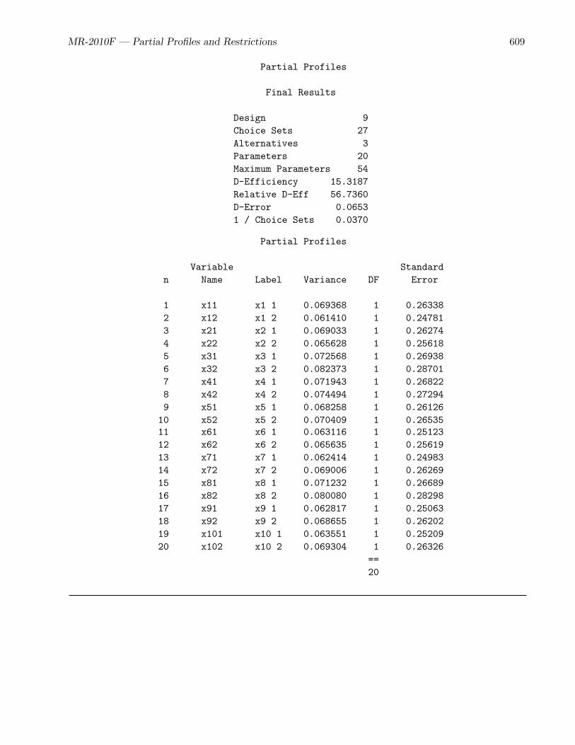
MR-2010F — Partial Profiles and Restrictions 609
Partial Profiles
Final Results
Design 9Choice Sets 27Alternatives 3Parameters 20Maximum Parameters 54D-Efficiency 15.3187Relative D-Eff 56.7360D-Error 0.06531 / Choice Sets 0.0370
Partial Profiles
Variable Standardn Name Label Variance DF Error
1 x11 x1 1 0.069368 1 0.263382 x12 x1 2 0.061410 1 0.247813 x21 x2 1 0.069033 1 0.262744 x22 x2 2 0.065628 1 0.256185 x31 x3 1 0.072568 1 0.269386 x32 x3 2 0.082373 1 0.287017 x41 x4 1 0.071943 1 0.268228 x42 x4 2 0.074494 1 0.272949 x51 x5 1 0.068258 1 0.2612610 x52 x5 2 0.070409 1 0.2653511 x61 x6 1 0.063116 1 0.2512312 x62 x6 2 0.065635 1 0.2561913 x71 x7 1 0.062414 1 0.2498314 x72 x7 2 0.069006 1 0.2626915 x81 x8 1 0.071232 1 0.2668916 x82 x8 2 0.080080 1 0.2829817 x91 x9 1 0.062817 1 0.2506318 x92 x9 2 0.068655 1 0.2620219 x101 x10 1 0.063551 1 0.2520920 x102 x10 2 0.069304 1 0.26326
==20
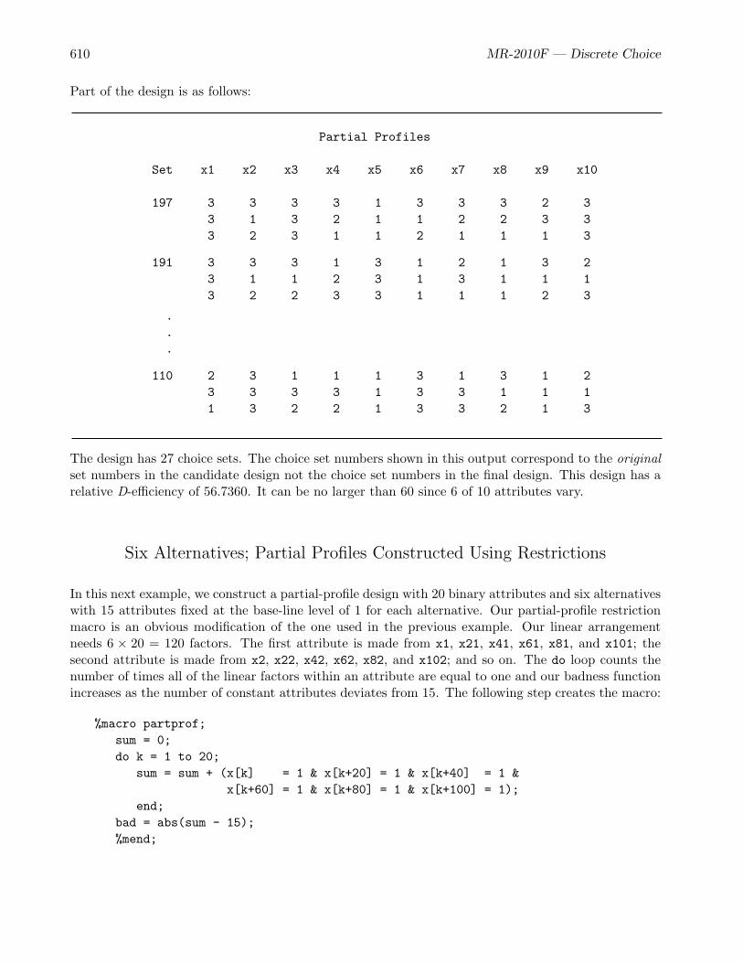
610 MR-2010F — Discrete Choice
Part of the design is as follows:
Partial Profiles
Set x1 x2 x3 x4 x5 x6 x7 x8 x9 x10
197 3 3 3 3 1 3 3 3 2 33 1 3 2 1 1 2 2 3 33 2 3 1 1 2 1 1 1 3
191 3 3 3 1 3 1 2 1 3 23 1 1 2 3 1 3 1 1 13 2 2 3 3 1 1 1 2 3
.
.
.
110 2 3 1 1 1 3 1 3 1 23 3 3 3 1 3 3 1 1 11 3 2 2 1 3 3 2 1 3
The design has 27 choice sets. The choice set numbers shown in this output correspond to the originalset numbers in the candidate design not the choice set numbers in the final design. This design has arelative D-efficiency of 56.7360. It can be no larger than 60 since 6 of 10 attributes vary.
Six Alternatives; Partial Profiles Constructed Using Restrictions
In this next example, we construct a partial-profile design with 20 binary attributes and six alternativeswith 15 attributes fixed at the base-line level of 1 for each alternative. Our partial-profile restrictionmacro is an obvious modification of the one used in the previous example. Our linear arrangementneeds 6 × 20 = 120 factors. The first attribute is made from x1, x21, x41, x61, x81, and x101; thesecond attribute is made from x2, x22, x42, x62, x82, and x102; and so on. The do loop counts thenumber of times all of the linear factors within an attribute are equal to one and our badness functionincreases as the number of constant attributes deviates from 15. The following step creates the macro:
%macro partprof;sum = 0;do k = 1 to 20;
sum = sum + (x[k] = 1 & x[k+20] = 1 & x[k+40] = 1 &x[k+60] = 1 & x[k+80] = 1 & x[k+100] = 1);
end;bad = abs(sum - 15);%mend;

MR-2010F — Partial Profiles and Restrictions 611
The %MktEx macro is run as follows:
%mktex(2 ** 120, /* 120 two-level factors */n=300, /* 300 runs */order=random, /* loop over columns in a random order */out=cand, /* output design */restrictions=partprof, /* name of restrictions macro */seed=424, /* random number seed */maxtime=0, /* stop once design conforms */options=largedesign /* make large design more quickly */
nosort /* do not sort output design */resrep /* detailed report on restrictions */quickr /* very quick run with random init */nox) /* suppress x1, x2, ... creation */
This step requests 120 binary factors and 300 runs. We specify order=random so that the columnsare looped over in a random order in the coordinate-exchange algorithm. You should always specifyorder=random with partial-profile designs. With a sequential order you tend to get nonvarying at-tributes paired with only nearby attributes. Several options are specified to make this step run quickly.With maxtime=0, only one design is created. With options=quickr, that one design is created withthe coordinate exchange algorithm and a random initialization. (The “r” in quickr stands for random.)The largedesign option allows %MktEx to stop as soon as it has imposed all restrictions. The resrepoption reports on the progress of imposing restrictions.
The first part of the output is as follows:
Algorithm Search History
Current BestDesign Row,Col D-Efficiency D-Efficiency Notes----------------------------------------------------------
1 Start 79.5699 Ran,Mut,Ann1 1 79.8384 14 Violations1 2 80.0541 12 Violations1 3 80.3047 14 Violations1 4 80.5649 15 Violations1 5 80.7840 13 Violations1 6 81.0383 12 Violations...
At the end of the first pass through the design we see the following warning:
WARNING: It may be impossible to meet all restrictions.
The macro never gets anywhere in imposing restrictions. Every row of the design has many restric-tion violations as shown by the output from the resrep (restrictions report) option. Always specifyoptions=resrep with complicated restrictions so you can look for things like this. When the macro is

612 MR-2010F — Discrete Choice
never succeeding in imposing restrictions, there is something wrong with the restrictions macro. Themacro we used is as follows:
%macro partprof;sum = 0;do k = 1 to 20;
sum = sum + (x[k] = 1 & x[k+20] = 1 & x[k+40] = 1 &x[k+60] = 1 & x[k+80] = 1 & x[k+100] = 1);
end;bad = abs(sum - 15);%mend;
It correctly evaluates the Boolean expression to determine whether an attribute is all one, and itcorrectly counts the number of such attributes. It also correctly sets bad to the absolute differencebetween the sum and 15, the desired number of constant attributes. Sometimes you get results like wejust saw when you made a logical mistake in programming the restrictions. For example, you mighthave written a set of restrictions that are impossible to satisfy. That is not the problem in this case.The problem in this case is the quantification of badness is not fine enough. You need to tell the macrowhenever it does something that moves it closer to an acceptable solution. Consider a potential choiceset that almost conforms to the restrictions such as the following:
Set x1 x2 x3 x4 x5 x6 x7 x8 x9 x10 x11 x12 x13 x14 x15 x16 x17 x18 x19 x20
1 2 1 1 1 2 2 1 1 1 1 1 1 2 1 1 1 1 1 1 12 1 2 1 2 2 1 1 1 1 1 1 2 1 1 1 1 1 1 11 1 2 1 1 2 2 1 1 1 1 1 2 1 1 1 1 1 1 11 1 2 1 2 2 1 1 1 1 1 1 1 1 1 1 1 1 1 12 1 1 1 1 1 2 1 1 1 1 1 1 1 1 1 1 1 1 11 1 1 1 1 1 1 1 1 1 1 1 1 1 1 1 1 1 1 1
The problem with this choice set is it has six nonconstant attributes instead of five. So bad = abs(14 -15) = 1. Now consider what happens when the macro changes the first attribute of the first alternativefrom 2 to 1. This is a change in the right direction because it moves the choice set closer to havingone more constant attribute. However, this change has no effect on the badness criterion. It is still1, because we still have six nonconstant attributes. We are not giving %MktEx enough informationabout when it is heading in the right direction. The %MktEx macro, without your restrictions macro tootherwise guide it, is guided by the goal of maximizing D-efficiency. It does not particularly want tomake partial-profile designs, because imposing all of those ties decreases statistical D-efficiency. Usingthe hill climbing analogy, %MktEx wants to climb Mount Everest; your restrictions macro needs to tellit to find the top of an island in the middle of a river valley. This is not where %MktEx would normallylook. If your restrictions macro is going to overcome the %MktEx macro’s normal goal, you have totrain it and more explicitly tell it where to look.
Training the %MktEx macro to find highly restricted designs is like training a dog. You have to bepersistent and consistent, and you need to watch it every second. You have to reward it whenever itdoes the right thing and you have to punish it for even thinking about doing the wrong thing. Whenit tears up your favorite slippers, you need to whack it over the head with a rolled up newspaper.∗ It
∗No actual dogs were harmed in the process of developing any of this software.
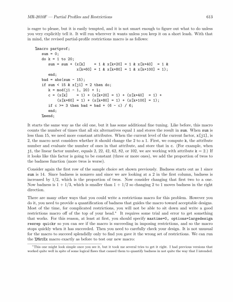
MR-2010F — Partial Profiles and Restrictions 613
is eager to please, but it is easily tempted, and it is not smart enough to figure out what to do unlessyou very explicitly tell it. It will run wherever it wants unless you keep it on a short leash. With thatin mind, the revised partial-profile restrictions macro is as follows:
%macro partprof;sum = 0;do k = 1 to 20;
sum = sum + (x[k] = 1 & x[k+20] = 1 & x[k+40] = 1 &x[k+60] = 1 & x[k+80] = 1 & x[k+100] = 1);
end;bad = abs(sum - 15);if sum < 15 & x[j1] = 2 then do;
k = mod(j1 - 1, 20) + 1;c = (x[k] = 1) + (x[k+20] = 1) + (x[k+40] = 1) +
(x[k+60] = 1) + (x[k+80] = 1) + (x[k+100] = 1);if c >= 3 then bad = bad + (6 - c) / 6;end;
%mend;
It starts the same way as the old one, but it has some additional fine tuning. Like before, this macrocounts the number of times that all six alternatives equal 1 and stores the result in sum. When sum isless than 15, we need more constant attributes. When the current level of the current factor, x[j1], is2, the macro next considers whether it should change the 2 to a 1. First, we compute k, the attributenumber and evaluate the number of ones in that attribute, and store that in c. (For example, whenj1, the linear factor number, equals 2, 22, 42, 62, 82, or 102, we are working with attribute k = 2.) Ifit looks like this factor is going to be constant (three or more ones), we add the proportion of twos tothe badness function (more twos is worse).
Consider again the first row of the sample choice set shown previously. Badness starts out as 1 sincesum is 14. Since badness is nonzero and since we are looking at a 2 in the first column, badness isincreased by 1/2, which is the proportion of twos. Now consider changing that first two to a one.Now badness is 1 + 1/3, which is smaller than 1 + 1/2 so changing 2 to 1 moves badness in the rightdirection.
There are many other ways that you could write a restrictions macro for this problem. However youdo it, you need to provide a quantification of badness that guides the macro toward acceptable designs.Most of the time, for complicated restrictions, you will not be able to sit down and write a goodrestrictions macro off of the top of your head.∗ It requires some trial and error to get somethingthat works. For this reason, at least at first, you should specify maxtime=0, options=largedesignresrep quickr so you can see if the macro is succeeding in imposing restrictions, and so the macrostops quickly when it has succeeded. Then you need to carefully check your design. It is not unusualfor the macro to succeed splendidly only to find you gave it the wrong set of restrictions. We can runthe %MktEx macro exactly as before to test our new macro:
∗This one might look simple once you see it, but it took me several tries to get it right. I had previous versions thatworked quite well in spite of some logical flaws that caused them to quantify badness in not quite the way that I intended.

614 MR-2010F — Discrete Choice
%mktex(2 ** 120, /* 120 two-level factors */n=300, /* 300 runs */order=random, /* loop over columns in a random order */out=cand, /* output design */restrictions=partprof, /* name of restrictions macro */seed=424, /* random number seed */maxtime=0, /* stop once design conforms */options=largedesign /* make large design more quickly */
nosort /* do not sort output design */resrep /* detailed report on restrictions */quickr /* very quick run with random init */nox) /* suppress x1, x2, ... creation */
Some of the output from the first pass through the design is as follows:
Algorithm Search History
Current BestDesign Row,Col D-Efficiency D-Efficiency Notes----------------------------------------------------------
1 Start 79.5699 Ran,Mut,Ann1 1 79.5426 0 Violations1 2 79.5904 1 Violations1 3 79.6679 4 Violations1 4 79.6601 2 Violations1 5 79.6136 0 Violations...1 100 70.7815 0 Violations1 101 70.6383 3.5 Violations1 102 70.4911 0 Violations...1 197 54.9906 2.5 Violations1 198 54.8216 2 Violations1 199 54.6956 3 Violations1 200 54.5982 4 Violations1 201 54.4009 3 Violations1 202 54.2690 5 Violations1 203 54.0316 1 Violations...1 297 37.1307 4 Violations1 298 36.9190 0 Violations1 299 36.7720 4 Violations1 300 36.5326 2 Violations
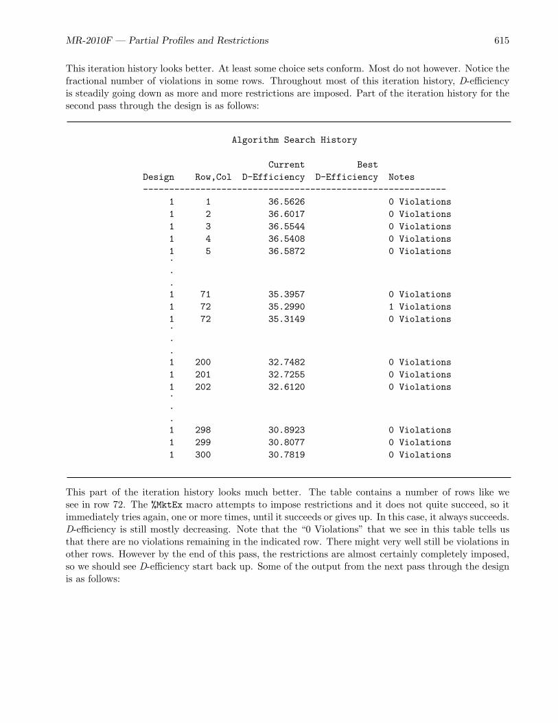
MR-2010F — Partial Profiles and Restrictions 615
This iteration history looks better. At least some choice sets conform. Most do not however. Notice thefractional number of violations in some rows. Throughout most of this iteration history, D-efficiencyis steadily going down as more and more restrictions are imposed. Part of the iteration history for thesecond pass through the design is as follows:
Algorithm Search History
Current BestDesign Row,Col D-Efficiency D-Efficiency Notes----------------------------------------------------------
1 1 36.5626 0 Violations1 2 36.6017 0 Violations1 3 36.5544 0 Violations1 4 36.5408 0 Violations1 5 36.5872 0 Violations...1 71 35.3957 0 Violations1 72 35.2990 1 Violations1 72 35.3149 0 Violations...1 200 32.7482 0 Violations1 201 32.7255 0 Violations1 202 32.6120 0 Violations...1 298 30.8923 0 Violations1 299 30.8077 0 Violations1 300 30.7819 0 Violations
This part of the iteration history looks much better. The table contains a number of rows like wesee in row 72. The %MktEx macro attempts to impose restrictions and it does not quite succeed, so itimmediately tries again, one or more times, until it succeeds or gives up. In this case, it always succeeds.D-efficiency is still mostly decreasing. Note that the “0 Violations” that we see in this table tells usthat there are no violations remaining in the indicated row. There might very well still be violations inother rows. However by the end of this pass, the restrictions are almost certainly completely imposed,so we should see D-efficiency start back up. Some of the output from the next pass through the designis as follows:

616 MR-2010F — Discrete Choice
Algorithm Search History
Current BestDesign Row,Col D-Efficiency D-Efficiency Notes----------------------------------------------------------
1 1 30.7883 0 Violations1 2 30.8000 0 Violations1 3 30.8232 0 Violations...1 100 32.2841 0 Violations1 101 32.3019 0 Violations1 102 32.3076 0 Violations...1 200 33.1653 0 Violations1 201 33.1732 0 Violations1 202 33.1784 0 Violations...1 298 33.8588 0 Violations1 299 33.8877 0 Violations1 300 33.8971 0 Violations
Now D-efficiency is increasing. The rest of the iteration history is as follows:
Algorithm Search History
Current BestDesign Row,Col D-Efficiency D-Efficiency Notes----------------------------------------------------------
1 1 1 33.8971 33.8971 Conforms1 1 53 33.8988 33.89881 1 60 33.9013 33.90131 1 6 33.9016 33.90161 End 33.9016
It is followed by the following messages:
NOTE: Stopping early, possibly before convergence, with a large design.

MR-2010F — Partial Profiles and Restrictions 617
Due to maxtime=0, options=largedesign quickr, the macro stops after it has completed one passthrough the design without encountering any restriction violations. Our final D-efficiency = 33.9016 isnot very high, but this is just a candidate set. Furthermore, this is a highly restricted design, so it isnot surprising that D-efficiency is not very high. We might want to iterate more and see if we can dobetter, but for now, let’s test the rest of our code. The %MktEx step took about 2.5 minutes. When themacro completes a full pass through the design without detecting any violations, it displays Conformsand switches from the options=resrep style to the normal iteration history style. The following stepsturn the linear arrangement into a choice design and eliminate duplicate choice sets:
%mktkey(6 20)
%mktroll(design=cand, key=key, out=rolled)
proc print; by set; id set; var x:; where set le 5; run;
%mktdups(generic, data=rolled, out=nodups, factors=x1-x20, nalts=6)
proc print data=nodups(obs=18); id set; by set; run;
The %MktKey macro is run to generate a Key data set with 6 rows, 20 columns and the variable namesx1 - x120. The Key data set, displayed in two panels, is as follows:
x1 x2 x3 x4 x5 x6 x7 x8 x9 x10
x1 x2 x3 x4 x5 x6 x7 x8 x9 x10x21 x22 x23 x24 x25 x26 x27 x28 x29 x30x41 x42 x43 x44 x45 x46 x47 x48 x49 x50x61 x62 x63 x64 x65 x66 x67 x68 x69 x70x81 x82 x83 x84 x85 x86 x87 x88 x89 x90x101 x102 x103 x104 x105 x106 x107 x108 x109 x110
x11 x12 x13 x14 x15 x16 x17 x18 x19 x20
x11 x12 x13 x14 x15 x16 x17 x18 x19 x20x31 x32 x33 x34 x35 x36 x37 x38 x39 x40x51 x52 x53 x54 x55 x56 x57 x58 x59 x60x71 x72 x73 x74 x75 x76 x77 x78 x79 x80x91 x92 x93 x94 x95 x96 x97 x98 x99 x100x111 x112 x113 x114 x115 x116 x117 x118 x119 x120
The %MktDups macro eliminated 70 choice sets with duplicate alternatives resulting in a candidate setwith 230 choice sets.

618 MR-2010F — Discrete Choice
The results of the last PROC PRINT, with the first three candidate choice sets, are as follows:
Set x1 x2 x3 x4 x5 x6 x7 x8 x9 x10 x11 x12 x13 x14 x15 x16 x17 x18 x19 x20
1 1 1 1 1 2 1 1 1 1 1 1 1 1 1 1 1 1 1 1 21 1 1 1 1 1 1 1 2 1 1 1 2 1 1 1 1 1 1 11 1 1 1 2 1 1 1 2 1 1 1 1 1 1 1 1 1 1 11 1 1 1 1 2 1 1 1 1 1 1 2 1 1 1 1 1 1 21 1 1 1 2 2 1 1 2 1 1 1 1 1 1 1 1 1 1 21 1 1 1 1 1 1 1 1 1 1 1 2 1 1 1 1 1 1 1
2 1 2 1 1 1 1 1 1 1 1 1 1 2 1 1 2 2 1 2 11 2 1 1 1 1 1 1 1 1 1 1 1 1 1 2 2 1 2 11 2 1 1 1 1 1 1 1 1 1 1 1 1 1 2 2 1 2 11 1 1 1 1 1 1 1 1 1 1 1 2 1 1 2 1 1 1 11 1 1 1 1 1 1 1 1 1 1 1 2 1 1 1 1 1 2 11 1 1 1 1 1 1 1 1 1 1 1 1 1 1 1 1 1 1 1
3 2 1 1 1 1 1 1 2 2 1 1 1 1 2 1 1 1 1 1 11 1 1 1 1 1 1 2 1 1 1 1 1 1 1 2 1 1 1 12 1 1 1 1 1 1 1 2 1 1 1 1 2 1 2 1 1 1 11 1 1 1 1 1 1 1 1 1 1 1 1 1 1 2 1 1 1 11 1 1 1 1 1 1 2 2 1 1 1 1 1 1 2 1 1 1 12 1 1 1 1 1 1 2 2 1 1 1 1 2 1 1 1 1 1 1
Each choice set has the correct number of nonconstant attributes. The following step runs the%ChoicEff macro to find a choice design:
%choiceff(data=nodups, /* candidate set of choice sets */model=class(x1-x20 / zero=first), /* main effects, first ref level*/seed=495, /* random number seed */maxiter=10, /* maximum iterations for each phase */nsets=18, /* number of choice sets */nalts=6, /* number of alternatives */options=nodups, /* no duplicate choice sets */beta=zero) /* assumed beta vector, Ho: b=0 */
proc print data=best; id set; by notsorted set; var x1-x20; run;
We set the reference level to the first level of each factor, which is the base-line level of 1. Some of theoutput is as follows:
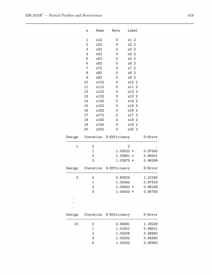
MR-2010F — Partial Profiles and Restrictions 619
n Name Beta Label
1 x12 0 x1 22 x22 0 x2 23 x32 0 x3 24 x42 0 x4 25 x52 0 x5 26 x62 0 x6 27 x72 0 x7 28 x82 0 x8 29 x92 0 x9 210 x102 0 x10 211 x112 0 x11 212 x122 0 x12 213 x132 0 x13 214 x142 0 x14 215 x152 0 x15 216 x162 0 x16 217 x172 0 x17 218 x182 0 x18 219 x192 0 x19 220 x202 0 x20 2
Design Iteration D-Efficiency D-Error----------------------------------------------
1 0 0 .1 1.02522 * 0.975402 1.03841 * 0.963013 1.03875 * 0.96269
Design Iteration D-Efficiency D-Error----------------------------------------------
2 0 0.82624 1.210301 1.02442 0.976162 1.03920 * 0.962283 1.04403 * 0.95783
.
.
.
Design Iteration D-Efficiency D-Error----------------------------------------------
10 0 0.84581 1.182291 1.01501 0.985212 1.03206 0.968933 1.04232 0.959404 1.04232 0.95940
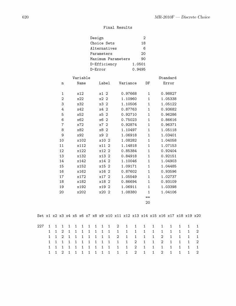
620 MR-2010F — Discrete Choice
Final Results
Design 2Choice Sets 18Alternatives 6Parameters 20Maximum Parameters 90D-Efficiency 1.0501D-Error 0.9495
Variable Standardn Name Label Variance DF Error
1 x12 x1 2 0.97668 1 0.988272 x22 x2 2 1.10960 1 1.053383 x32 x3 2 1.10506 1 1.051224 x42 x4 2 0.87763 1 0.936825 x52 x5 2 0.92710 1 0.962866 x62 x6 2 0.75023 1 0.866167 x72 x7 2 0.92874 1 0.963718 x82 x8 2 1.10497 1 1.051189 x92 x9 2 1.06918 1 1.0340110 x102 x10 2 1.08282 1 1.0405811 x112 x11 2 1.14818 1 1.0715312 x122 x12 2 0.85384 1 0.9240413 x132 x13 2 0.84918 1 0.9215114 x142 x14 2 1.10046 1 1.0490315 x152 x15 2 1.09171 1 1.0448516 x162 x16 2 0.87602 1 0.9359617 x172 x17 2 1.05549 1 1.0273718 x182 x18 2 0.86694 1 0.9310919 x192 x19 2 1.06911 1 1.0339820 x202 x20 2 1.08380 1 1.04106
==20
Set x1 x2 x3 x4 x5 x6 x7 x8 x9 x10 x11 x12 x13 x14 x15 x16 x17 x18 x19 x20
227 1 1 1 1 1 1 1 1 1 1 2 1 1 1 1 1 1 1 1 11 1 2 1 1 1 1 1 1 1 1 1 1 1 1 1 1 1 1 21 1 2 1 1 1 1 1 1 1 2 1 1 1 1 2 1 1 1 11 1 1 1 1 1 1 1 1 1 1 1 2 1 1 2 1 1 1 21 1 1 1 1 1 1 1 1 1 1 1 2 1 1 1 1 1 1 11 1 2 1 1 1 1 1 1 1 1 1 2 1 1 2 1 1 1 2

MR-2010F — Partial Profiles and Restrictions 621
187 1 1 1 1 1 1 1 1 1 2 1 2 1 1 1 1 1 2 1 11 1 1 2 1 1 1 1 1 1 1 2 1 1 2 1 1 1 1 11 1 1 2 1 1 1 1 1 2 1 1 1 1 2 1 1 2 1 11 1 1 2 1 1 1 1 1 2 1 2 1 1 1 1 1 1 1 11 1 1 2 1 1 1 1 1 1 1 1 1 1 2 1 1 2 1 11 1 1 1 1 1 1 1 1 1 1 1 1 1 1 1 1 1 1 1
.
.
.
191 1 1 2 1 2 1 1 1 1 1 1 1 1 1 1 1 1 1 1 11 1 2 1 1 1 1 1 1 1 1 1 1 1 1 1 1 2 1 11 1 2 1 1 1 1 2 1 1 1 1 1 2 1 1 1 1 1 11 1 1 1 1 1 1 2 1 1 1 1 1 2 1 1 1 1 1 11 1 1 1 2 1 1 2 1 1 1 1 1 1 1 1 1 2 1 11 1 1 1 2 1 1 1 1 1 1 1 1 2 1 1 1 2 1 1
Since the %ChoicEff macro did not have any problems, and the results look reasonable, it appearsthat we did everything right. Now we could try again, perhaps with more choice sets (say 400), andwe could iterate longer (say one hour), then we could make our final partial-profile choice design. Thisis illustrated in the following step:
%mktex(2 ** 120, /* 120 two-level factors */n=400, /* 400 runs */optiter=0, /* no PROC OPTEX iterations */tabiter=0, /* no OA initialization iterations */maxtime=60, /* at most 60 minutes per phase */order=random, /* loop over columns in a random order */out=cand, /* output design */restrictions=partprof, /* name of restrictions macro */seed=424, /* random number seed */maxstages=1, /* maximum number of algorithm stages */options=largedesign /* make large design more quickly */
nosort) /* do not sort output design */
The results of this step are not shown.
To recap, the first restrictions macro correctly differentiated between acceptable and unacceptablechoice sets, but it provided %MktEx with no guidance or direction on how to find acceptable choice sets.Hence, the first macro did not work. The second macro corrected this problem by “nudging” %MktExin the right direction. The restrictions macro looked for attributes that appear to be heading towardconstant and created a penalty function that encouraged %MktEx to make those attributes constant.Next, we will look at another way of writing a restrictions macro for this problem. There is nothingsubtle about this next approach. This next macro uses the whack-it-over-the-head-with-a-rolled-up-newspaper approach. Sometimes you need to tell %MktEx that a restriction is really important bystrongly eliminating that source of badness. In this case, our macro strongly eliminates twos from thedesign until the restriction violations go away. This is illustrated in the following steps:
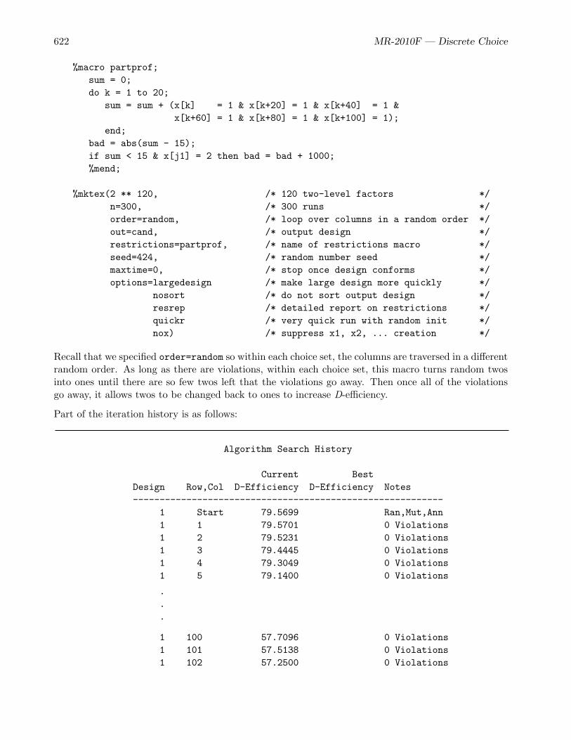
622 MR-2010F — Discrete Choice
%macro partprof;sum = 0;do k = 1 to 20;
sum = sum + (x[k] = 1 & x[k+20] = 1 & x[k+40] = 1 &x[k+60] = 1 & x[k+80] = 1 & x[k+100] = 1);
end;bad = abs(sum - 15);if sum < 15 & x[j1] = 2 then bad = bad + 1000;%mend;
%mktex(2 ** 120, /* 120 two-level factors */n=300, /* 300 runs */order=random, /* loop over columns in a random order */out=cand, /* output design */restrictions=partprof, /* name of restrictions macro */seed=424, /* random number seed */maxtime=0, /* stop once design conforms */options=largedesign /* make large design more quickly */
nosort /* do not sort output design */resrep /* detailed report on restrictions */quickr /* very quick run with random init */nox) /* suppress x1, x2, ... creation */
Recall that we specified order=random so within each choice set, the columns are traversed in a differentrandom order. As long as there are violations, within each choice set, this macro turns random twosinto ones until there are so few twos left that the violations go away. Then once all of the violationsgo away, it allows twos to be changed back to ones to increase D-efficiency.
Part of the iteration history is as follows:
Algorithm Search History
Current BestDesign Row,Col D-Efficiency D-Efficiency Notes----------------------------------------------------------
1 Start 79.5699 Ran,Mut,Ann1 1 79.5701 0 Violations1 2 79.5231 0 Violations1 3 79.4445 0 Violations1 4 79.3049 0 Violations1 5 79.1400 0 Violations
.
.
.
1 100 57.7096 0 Violations1 101 57.5138 0 Violations1 102 57.2500 0 Violations
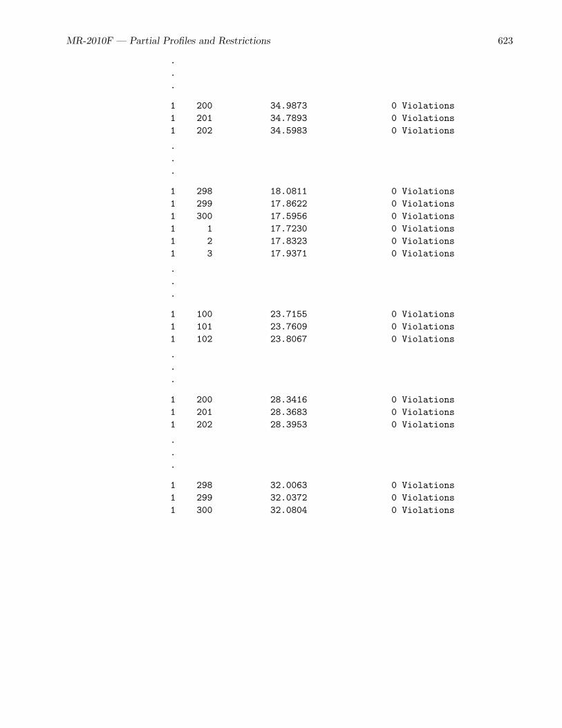
MR-2010F — Partial Profiles and Restrictions 623
.
.
.
1 200 34.9873 0 Violations1 201 34.7893 0 Violations1 202 34.5983 0 Violations
.
.
.
1 298 18.0811 0 Violations1 299 17.8622 0 Violations1 300 17.5956 0 Violations1 1 17.7230 0 Violations1 2 17.8323 0 Violations1 3 17.9371 0 Violations
.
.
.
1 100 23.7155 0 Violations1 101 23.7609 0 Violations1 102 23.8067 0 Violations
.
.
.
1 200 28.3416 0 Violations1 201 28.3683 0 Violations1 202 28.3953 0 Violations
.
.
.
1 298 32.0063 0 Violations1 299 32.0372 0 Violations1 300 32.0804 0 Violations

624 MR-2010F — Discrete Choice
1 1 1 32.0804 32.0804 Conforms1 1 13 32.0873 32.08731 1 27 32.0950 32.09501 1 105 32.0981 32.09811 1 103 32.1020 32.10201 1 113 32.1032 32.10321 1 65 32.1096 32.10961 1 106 32.1116 32.11161 1 86 32.1159 32.11591 1 43 32.1163 32.11631 1 47 32.1193 32.11931 1 45 32.1232 32.12321 1 3 32.1294 32.12941 1 53 32.1295 32.12951 1 107 32.1344 32.13441 1 6 32.1366 32.13661 1 73 32.1372 32.13721 End 32.1372
With this approach, all violations in each row are eliminated in the first pass through the design. Themacro quits after the end of the second pass, when it has completed an entire pass without encounteringany restriction violations.
Call the first approach the “nudge” approach and the second approach the “whack” approach. Thenudge approach starts with D-efficiency on the order of 80% for the random design. After one completepass, imposing many but not all restrictions, D-efficiency is down around 37%. After another pass andimposing all restrictions, it is down to around 31%. Then it creeps back up to 34%. D-efficiency forthe choice design is approximately 1.05. The whack approach starts with the same random design (dueto the same random number seed) and with the same D-efficiency on the order of 80%. Then after onepass of severe restriction imposition, D-efficiency drops to 18%. The nudge approach asks “are you agood two or a bad two?” and then acts accordingly. In contrast, when the whack approach sees a two,it whacks it—no questions asked. There is no subtle nudging in the whack approach, and initially, itover corrects to impose restrictions. Hence, the design it makes at the end of the first pass is not verygood, but once all of the restrictions are in place, D-efficiency quickly recovers to 32%. This is notquite as high as the nudge approach, but the nudge approach had one more complete pass through thedesign.
It is natural to ask, which approach is better? There are many ways to get %MktEx to impose therestrictions. It is not clear that one is better than the other. Our goal here is to use %MktEx to createa set of candidates for the %ChoicEff macro to search. Any restrictions macro that accomplishes thisshould be fine. Writing a macro that uses the whack approach is probably a bit easier. However, thereis always some worry that the initial over correction might not be a good thing. In contrast, subtlenudging takes longer to get to the point of all restrictions being met, and you have to be a bit creativesometimes to write nudges that actually work. Sometimes you need to combine both approaches—whack it to take care of one set of restrictions then nudge it in the right direction for a secondary setof restrictions. This is all part of the art of sophisticated experimental design. Note that it is not thefact that we used a large penalty of 1000 that makes this approach an example of the whack approach.It is the whack approach because we strongly over-corrected every violation.

MR-2010F — Partial Profiles and Restrictions 625
The differential weighting of the components of badness is another very important strategy to keep inmind. When there is more than one aspect to the set of restrictions, they sometimes trade off againsteach other. Every time %MktEx fixes one thing, something else gets worse. Differentially weighting thecomponents, as we did in the partprof macro, can greatly help avoid this. The first component, bad= abs(sum - 15); sets badness to values in the range 0 to 15. The next component if sum < 15 &x[j1] = 2 then bad = bad + 1000; adds contributions in the thousands. %MktEx will never increasethe second component to decrease the first. This gives %MktEx something of a two-stage functionality.At first, it worries about eliminating twos and also having the right number, but mostly it eliminatestwos. Once it eliminates the most-penalized source of badness then it can concentrate on the remainingsource, as long as it does not bring back any of the badness it previously eliminated. Often times, itdoes not matter which component you weight the most, nor does it matter how much you weight them,as long as each component has a differential weight.
We could run the %ChoicEff macro again to see what the final D-efficiency is like before as follows:
%choiceff(data=nodups, /* candidate set of choice sets */model=class(x1-x20 / zero=first), /* main effects, first ref level*/seed=495, /* random number seed */maxiter=10, /* maximum iterations for each phase */nsets=18, /* number of choice sets */nalts=6, /* number of alternatives */options=nodups, /* no duplicate choice sets */beta=zero) /* assumed beta vector, Ho: b=0 */
The summary table is as follows:
Final Results
Design 3Choice Sets 18Alternatives 6Parameters 20Maximum Parameters 90D-Efficiency 1.0531D-Error 0.9495
These results are similar to those from before. We could also specify the standardized orthogonalcontrast coding as follows:
%choiceff(data=nodups, /* candidate set of choice sets */model=class(x1-x20 / sta),/* model with stdzd orthogonal coding */seed=495, /* random number seed */maxiter=10, /* maximum iterations for each phase */nsets=18, /* number of choice sets */nalts=6, /* number of alternatives */options=nodups /* no duplicate choice sets */
relative, /* display relative D-efficiency */beta=zero) /* assumed beta vector, Ho: b=0 */

626 MR-2010F — Discrete Choice
The summary table is as follows:
Final Results
Design 3Choice Sets 18Alternatives 6Parameters 20Maximum Parameters 90D-Efficiency 4.2126Relative D-Eff 23.4032D-Error 0.23741 / Choice Sets 0.0556
D-efficiency is 23.4032. The largest it could possibly be is 25 since 5 of 20 attributes (25%) vary.
Five-Level Factors; Partial Profiles Constructed Using Restrictions
This next example extends what we discussed in the previous example and constructs a somewhatdifferent style of partial-profile design. This design has five alternatives and 15 five-level factors, fiveof which vary in each choice set. Unlike the previous example, however, the constant factors are notall at the base-line level. The constant factors can have any of the levels, and we use the first factorwithin each attribute when we check the restrictions. The partial-profile restrictions macro along with%MktEx code, which uses the same basic option set that we used in the previous example, is as follows:
%macro partprof;sum = 0;do k = 1 to 15;
sum = sum + (x[k+15] = x[k] & x[k+30] = x[k] &x[k+45] = x[k] & x[k+60] = x[k]);
end;bad = abs(sum - 10);if sum < 10 & x[j1] ^= x[mod(j1 - 1, 15) + 1] then bad = bad + 1000;%mend;
%mktex(5 ** 75, /* 75 five-level factors */n=400, /* 400 runs */order=random, /* loop over columns in a random order */out=cand, /* output design */restrictions=partprof, /* name of restrictions macro */seed=472, /* random number seed */maxtime=0, /* stop once design conforms */options=largedesign /* make large design more quickly */
nosort /* do not sort output design */resrep /* detailed report on restrictions */quickr /* very quick run with random init */nox) /* suppress x1, x2, ... creation */

MR-2010F — Partial Profiles and Restrictions 627
The macro counts the number of times all of the linear factors in a choice set attribute are constantwithin choice set, that is they equal the level of the first linear factor in the attribute, then it computesbadness in the customary way. Also like before, when not all restrictions are met, any level that is notequal to the first factor within its attribute is heavily penalized. The macro uses the “whack” approachto impose constant attributes. Some of the iteration history is as follows:
Algorithm Search History
Current BestDesign Row,Col D-Efficiency D-Efficiency Notes----------------------------------------------------------
1 1 58.6862 0 Violations1 2 58.7150 1 Violations1 3 58.6810 2 Violations
.
.
.
1 100 56.0416 5 Violations1 101 55.9496 0 Violations1 102 55.8855 4 Violations
.
.
.
1 200 48.0539 3 Violations1 201 47.9776 3 Violations1 202 47.9279 4 Violations
.
.
.
1 300 38.9711 0 Violations1 301 38.8695 4 Violations1 302 38.7805 3 Violations
.
.
.
1 398 30.4723 2 Violations1 399 30.4075 2 Violations1 400 30.3169 2 Violations1 1 30.4110 0 Violations1 2 30.4491 0 Violations1 3 30.5001 0 Violations
.
.
.

628 MR-2010F — Discrete Choice
1 73 32.8050 2 Violations1 73 32.8708 0 Violations1 74 32.8840 0 Violations1 75 32.8518 1 Violations1 75 32.8845 0 Violations
.
.
.
1 398 34.9958 0 Violations1 399 35.0104 0 Violations1 400 34.9901 0 Violations1 1 35.0015 0 Violations1 2 35.0133 0 Violations1 3 35.0337 0 Violations
.
.
.
1 398 43.0865 0 Violations1 399 43.1054 0 Violations1 400 43.1304 0 Violations1 1 1 43.1304 43.1304 Conforms1 1 42 43.1311 43.13111 1 17 43.1338 43.13381 End 43.1305
This iteration history has a pattern very similar to what we saw in the previous example with thenudge approach. In the first pass through the design, not all restrictions are met. Even the whackapproach does not guarantee that all restrictions get met right away. In the second pass, some rowsare processed more than once until all restrictions are met. We can see that in choice sets 73 and 75.By the end of the second pass, all restrictions are met (efficiency starts back up), %MktEx realizes allrestrictions are met at the end of the third pass, and then it stops. The %MktEx macro iterates longer ifwe do not specify options=largedesign, but for now when you are testing a new restrictions macro,it is good to check the results before %MktEx spends a long time iterating. The following steps createa choice design from this linear candidate set in the familiar way:

MR-2010F — Partial Profiles and Restrictions 629
%mktkey(5 15)
%mktroll(design=cand, key=key, out=rolled)
%mktdups(generic, data=rolled, out=nodups, factors=x1-x15, nalts=5)
%choiceff(data=nodups, /* candidate set of choice sets */model=class(x1-x15 / sta),/* model with stdz orthogonal coding */seed=513, /* random number seed */maxiter=10, /* maximum iterations for each phase */nsets=15, /* number of choice sets */nalts=5, /* number of alternatives */options=nodups /* no duplicate choice sets */
relative, /* display relative D-efficiency */beta=zero) /* assumed beta vector, Ho: b=0 */
proc print data=best(obs=15); id set; by notsorted set; var x1-x15; run;
The key with 5 rows, 15 columns and the variable names x1 - x75 is as follows:
x1 x2 x3 x4 x5 x6 x7 x8 x9 x10 x11 x12 x13 x14 x15
x1 x2 x3 x4 x5 x6 x7 x8 x9 x10 x11 x12 x13 x14 x15x16 x17 x18 x19 x20 x21 x22 x23 x24 x25 x26 x27 x28 x29 x30x31 x32 x33 x34 x35 x36 x37 x38 x39 x40 x41 x42 x43 x44 x45x46 x47 x48 x49 x50 x51 x52 x53 x54 x55 x56 x57 x58 x59 x60x61 x62 x63 x64 x65 x66 x67 x68 x69 x70 x71 x72 x73 x74 x75
Skipping the %ChoicEff macro output for a moment, part of the choice design is as follows:
Set x1 x2 x3 x4 x5 x6 x7 x8 x9 x10 x11 x12 x13 x14 x15
33 5 5 4 5 2 1 4 2 3 5 5 2 5 3 15 1 3 1 2 1 4 4 3 5 1 2 5 3 15 5 3 4 2 1 4 5 3 5 2 2 5 3 15 1 1 2 2 1 4 1 3 5 5 2 5 3 15 2 5 3 2 1 4 3 3 5 3 2 5 3 1
291 3 2 3 1 2 4 5 4 2 4 3 1 1 2 43 2 3 1 2 4 5 3 3 4 3 1 5 4 43 2 3 1 2 4 4 2 5 4 3 1 3 5 43 2 3 1 2 4 5 5 2 4 3 1 4 3 43 2 3 1 2 4 4 1 4 4 3 1 1 1 4

630 MR-2010F — Discrete Choice
186 3 4 3 3 5 2 1 1 4 1 3 1 1 3 53 4 5 3 5 2 5 2 4 2 3 1 1 3 43 4 2 3 5 2 3 1 4 4 3 1 1 3 23 4 1 3 5 2 4 3 4 5 3 1 1 3 53 4 4 3 5 2 4 5 4 3 3 1 1 3 3
The pattern of constant and nonconstant attributes looks correct: 10 constant and 5 nonconstantattributes per choice set. Furthermore, the constant attributes have the full range of levels. The lastpart of the output from the %ChoicEff macro is as follows:
Final Results
Design 9Choice Sets 15Alternatives 5Parameters 60Maximum Parameters 60D-Efficiency 2.3286Relative D-Eff 15.5243D-Error 0.42941 / Choice Sets 0.0667
Variable Standardn Name Label Variance DF Error
1 x11 x1 1 1.24427 1 1.115472 x12 x1 2 1.37689 1 1.173413 x13 x1 3 1.62664 1 1.275404 x14 x1 4 1.25242 1 1.119125 x21 x2 1 1.06398 1 1.031496 x22 x2 2 2.50082 1 1.581407 x23 x2 3 1.54702 1 1.243798 x24 x2 4 1.00564 1 1.002829 x31 x3 1 1.68441 1 1.2978510 x32 x3 2 0.72847 1 0.8535111 x33 x3 3 1.58669 1 1.2596412 x34 x3 4 1.36204 1 1.1670713 x41 x4 1 1.57492 1 1.2549614 x42 x4 2 2.40504 1 1.5508215 x43 x4 3 2.07707 1 1.4412016 x44 x4 4 1.37807 1 1.1739117 x51 x5 1 1.84721 1 1.3591218 x52 x5 2 3.63100 1 1.9055219 x53 x5 3 2.87391 1 1.6952620 x54 x5 4 0.87844 1 0.93725
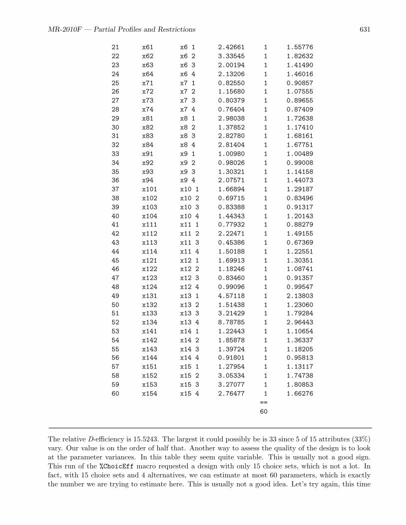
MR-2010F — Partial Profiles and Restrictions 631
21 x61 x6 1 2.42661 1 1.5577622 x62 x6 2 3.33545 1 1.8263223 x63 x6 3 2.00194 1 1.4149024 x64 x6 4 2.13206 1 1.4601625 x71 x7 1 0.82550 1 0.9085726 x72 x7 2 1.15680 1 1.0755527 x73 x7 3 0.80379 1 0.8965528 x74 x7 4 0.76404 1 0.8740929 x81 x8 1 2.98038 1 1.7263830 x82 x8 2 1.37852 1 1.1741031 x83 x8 3 2.82780 1 1.6816132 x84 x8 4 2.81404 1 1.6775133 x91 x9 1 1.00980 1 1.0048934 x92 x9 2 0.98026 1 0.9900835 x93 x9 3 1.30321 1 1.1415836 x94 x9 4 2.07571 1 1.4407337 x101 x10 1 1.66894 1 1.2918738 x102 x10 2 0.69715 1 0.8349639 x103 x10 3 0.83388 1 0.9131740 x104 x10 4 1.44343 1 1.2014341 x111 x11 1 0.77932 1 0.8827942 x112 x11 2 2.22471 1 1.4915543 x113 x11 3 0.45386 1 0.6736944 x114 x11 4 1.50188 1 1.2255145 x121 x12 1 1.69913 1 1.3035146 x122 x12 2 1.18246 1 1.0874147 x123 x12 3 0.83460 1 0.9135748 x124 x12 4 0.99096 1 0.9954749 x131 x13 1 4.57118 1 2.1380350 x132 x13 2 1.51438 1 1.2306051 x133 x13 3 3.21429 1 1.7928452 x134 x13 4 8.78785 1 2.9644353 x141 x14 1 1.22443 1 1.1065454 x142 x14 2 1.85878 1 1.3633755 x143 x14 3 1.39724 1 1.1820556 x144 x14 4 0.91801 1 0.9581357 x151 x15 1 1.27954 1 1.1311758 x152 x15 2 3.05334 1 1.7473859 x153 x15 3 3.27077 1 1.8085360 x154 x15 4 2.76477 1 1.66276
==60
The relative D-efficiency is 15.5243. The largest it could possibly be is 33 since 5 of 15 attributes (33%)vary. Our value is on the order of half that. Another way to assess the quality of the design is to lookat the parameter variances. In this table they seem quite variable. This is usually not a good sign.This run of the %ChoicEff macro requested a design with only 15 choice sets, which is not a lot. Infact, with 15 choice sets and 4 alternatives, we can estimate at most 60 parameters, which is exactlythe number we are trying to estimate here. This is usually not a good idea. Let’s try again, this time

632 MR-2010F — Discrete Choice
with 30 choice sets. The following step finds the design:
%choiceff(data=nodups, /* candidate set of choice sets */model=class(x1-x15 / sta),/* model with stdz orthogonal coding */seed=513, /* random number seed */maxiter=10, /* maximum iterations for each phase */nsets=30, /* number of choice sets */nalts=5, /* number of alternatives */options=nodups /* no duplicate choice sets */
relative, /* display relative D-efficiency */beta=zero) /* assumed beta vector, Ho: b=0 */
The new results and variance tables are as follows:
Partial Profiles
Final Results
Design 1Choice Sets 30Alternatives 5Parameters 60Maximum Parameters 120D-Efficiency 7.7251Relative D-Eff 25.7503D-Error 0.12941 / Choice Sets 0.0333
Partial Profiles
Variable Standardn Name Label Variance DF Error
1 x11 x1 1 0.16200 1 0.402502 x12 x1 2 0.15231 1 0.390273 x13 x1 3 0.15801 1 0.397514 x14 x1 4 0.18802 1 0.433615 x21 x2 1 0.20554 1 0.453376 x22 x2 2 0.15363 1 0.391967 x23 x2 3 0.16931 1 0.411478 x24 x2 4 0.17124 1 0.413819 x31 x3 1 0.14382 1 0.3792410 x32 x3 2 0.13760 1 0.3709411 x33 x3 3 0.19570 1 0.4423812 x34 x3 4 0.15172 1 0.3895213 x41 x4 1 0.13177 1 0.3630014 x42 x4 2 0.13093 1 0.3618515 x43 x4 3 0.13788 1 0.37133

MR-2010F — Partial Profiles and Restrictions 633
16 x44 x4 4 0.15115 1 0.3887817 x51 x5 1 0.14697 1 0.3833618 x52 x5 2 0.12922 1 0.3594719 x53 x5 3 0.12505 1 0.3536220 x54 x5 4 0.17476 1 0.4180421 x61 x6 1 0.15004 1 0.3873522 x62 x6 2 0.17357 1 0.4166123 x63 x6 3 0.12204 1 0.3493424 x64 x6 4 0.13766 1 0.3710225 x71 x7 1 0.18417 1 0.4291526 x72 x7 2 0.16833 1 0.4102727 x73 x7 3 0.13836 1 0.3719728 x74 x7 4 0.14091 1 0.3753829 x81 x8 1 0.16784 1 0.4096930 x82 x8 2 0.16454 1 0.4056431 x83 x8 3 0.14048 1 0.3748132 x84 x8 4 0.17935 1 0.4234933 x91 x9 1 0.17887 1 0.4229334 x92 x9 2 0.17178 1 0.4144735 x93 x9 3 0.18717 1 0.4326336 x94 x9 4 0.16287 1 0.4035737 x101 x10 1 0.17880 1 0.4228438 x102 x10 2 0.15523 1 0.3940039 x103 x10 3 0.15494 1 0.3936240 x104 x10 4 0.15128 1 0.3889441 x111 x11 1 0.15144 1 0.3891642 x112 x11 2 0.19196 1 0.4381343 x113 x11 3 0.18085 1 0.4252644 x114 x11 4 0.17372 1 0.4168045 x121 x12 1 0.16954 1 0.4117546 x122 x12 2 0.19912 1 0.4462347 x123 x12 3 0.16908 1 0.4112048 x124 x12 4 0.15868 1 0.3983449 x131 x13 1 0.17289 1 0.4158050 x132 x13 2 0.19481 1 0.4413851 x133 x13 3 0.21682 1 0.4656452 x134 x13 4 0.17501 1 0.4183453 x141 x14 1 0.15621 1 0.3952454 x142 x14 2 0.13804 1 0.3715455 x143 x14 3 0.13537 1 0.3679356 x144 x14 4 0.16000 1 0.4000057 x151 x15 1 0.14634 1 0.3825458 x152 x15 2 0.16575 1 0.4071259 x153 x15 3 0.14842 1 0.3852560 x154 x15 4 0.17341 1 0.41643
==60

634 MR-2010F — Discrete Choice
This looks much better. The variances are smaller and more uniform and relative D-efficiency is larger.Note that it is good to run the %MktEx macro again without options=largedesign and let it iteratemore before making the final choice design.
Next, we will investigate another thing you can try. Typically, the %MktEx macro is run so that it loopsover all of the columns in a row, and then it goes on to the next row. Alternatively, it can work withpairs of columns at one time using the exchange=2 option. Working with pairs of columns instead ofsingle columns is always much slower, but sometimes it can make better designs. The following stepscreate the design:
%macro partprof;sum = 0;do k = 1 to 15;
sum = sum + (x[k+15] = x[k] & x[k+30] = x[k] &x[k+45] = x[k] & x[k+60] = x[k]);
end;bad = abs(sum - 10);if sum < 10 then do;
if x[j1] ^= x[mod(j1 - 1, 15) + 1] then bad = bad + 1000;if x[j2] ^= x[mod(j2 - 1, 15) + 1] then bad = bad + 1000;end;
%mend;
%mktex(5 ** 75, /* 75 five-level factors */n=400, /* 400 runs */optiter=0, /* no PROC OPTEX iterations */tabiter=0, /* no OA initialization iterations */maxtime=720, /* at most 720 minutes per phase */order=random=15, /* pairwise exchanges within */
/* nonconstant attributes */out=sasuser.cand, /* output design stored permanently */restrictions=partprof, /* name of restrictions macro */seed=472, /* random number seed */exchange=2, /* pairwise exchanges */maxstages=1, /* maximum number of algorithm stages */options=largedesign /* make large design more quickly */
nosort /* do not sort output design */resrep /* detailed report on restrictions */nox) /* suppress x1, x2, ... creation */
The initial quantification of badness is the same. Like before, nonconforming levels are whacked.This time however, they are whacked in two ways—when j1, the primary column index points toa nonconstant level, and when j2, the secondary column index for the pairwise exchange indexes anonconstant level. In the %MktEx invocation, we now see maxtime=720 so that %MktEx can run overnight for 12 hours (or 720 minutes). We also see exchange=2 for pairwise exchanges. The output dataset is stored as a permanent SAS data set in the sasuser library. If we search for 12 hours for a design,we want to make sure it is there for us if we accidentally trip over the power cord in the morning beforewe have our coffee. See page 309 for more information about permanent SAS data sets.

MR-2010F — Partial Profiles and Restrictions 635
There is one more option in this example that we have not used previously, order=random=15. Thisis a special variation on order=random for pairwise exchanges in partial-profile designs. Before thisoption is explained, here is a bit of background. Sequential pairwise exchanges for m factors workslike this: %MktEx sets j1 = 1, 2, 3, ..., m and j2 = j1 + 1, j1 + 2, ..., m. Together, the variablesj1 and j2 loop over all pairs of columns. Random pairwise exchanges work like this: this: %MktExsets j1 = random permutation(1, 2, 3, ..., m) and j2 = random permutation(j1 + 1, j1 + 2, ..., m).Together, the variables j1 and j2 loop over all pairs of columns but in a random order. For partialprofiles, pairwise exchanges are appealing, because sometimes there is a lot to be gained by having twovalues change at once. However, it does not make sense to consider simultaneously changing the levelof a nonconstant attribute and the level of a constant attribute, nor does it make sense to considerpairwise exchanges within constant attributes. Random exchange with a value of 15 specified workslike this: %MktEx sets j1 = random permutation(1, 2, 3, ..., m) and j2 is set to a sequential list of theother factors in the same attribute as j1. For example, when j1 = 18, which means j1 is indexing thesecond alternative (18 is in the second block of 15 factors) for the third attribute (18 is 3 beyond thefifteenth factor, which is the end of the first block), then j2 = 3, 18, 33, 48, and 63 for a nonconstantthird attribute (which index the 5 factors that make up the third attribute) and j2 = j1 for constantattributes. This does pairwise exchanges but only within nonconstant attributes. This eliminates a lotof unproductive pairs from consideration.
A small part of the iteration history is as follows:
Algorithm Search History
Current BestDesign Row,Col D-Efficiency D-Efficiency Notes----------------------------------------------------------
1 Start 58.6611 Ran,Mut,Ann1 1 58.6962 0 Violations1 2 58.7140 0 Violations1 3 58.7171 1 Violations1 4 58.7076 1 Violations1 5 58.7269 2 Violations1 6 58.6943 2 Violations
.
.
.
1 398 31.1040 0 Violations1 399 31.0346 3 Violations1 400 30.9260 1 Violations1 1 31.0114 0 Violations1 2 31.0566 0 Violations1 3 31.1412 0 Violations
.
.
.

636 MR-2010F — Discrete Choice
1 48 32.6265 0 Violations1 49 32.6150 3 Violations1 49 32.5890 1 Violations1 49 32.6547 0 Violations1 50 32.7205 0 Violations
.
.
.
1 398 34.7853 0 Violations1 399 34.7463 0 Violations1 400 34.7763 0 Violations1 1 34.8061 0 Violations1 2 34.8381 0 Violations1 3 34.8520 0 Violations
.
.
.
1 398 43.2881 0 Violations1 399 43.2774 0 Violations1 400 43.3051 0 Violations1 1 1 43.3051 43.3051 Conforms1 1 72 43.3085 43.30851 1 26 43.3105 43.31051 1 41 43.3113 43.3113
.
.
.
1 154 7 50.0432 50.04321 176 1 50.0432 50.04321 217 17 50.0432 50.04321 End 50.0432
It is followed by the following messages:
NOTE: Stopping early, possibly before convergence, with a large design.NOTE: Quitting the algorithm search step after 720.01 minutes and 22 designs.
The following steps make and evaluate the choice design:
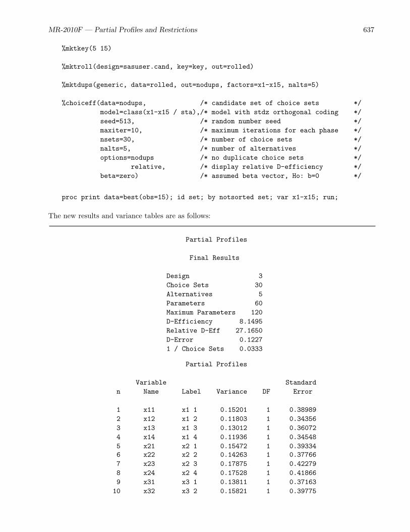
MR-2010F — Partial Profiles and Restrictions 637
%mktkey(5 15)
%mktroll(design=sasuser.cand, key=key, out=rolled)
%mktdups(generic, data=rolled, out=nodups, factors=x1-x15, nalts=5)
%choiceff(data=nodups, /* candidate set of choice sets */model=class(x1-x15 / sta),/* model with stdz orthogonal coding */seed=513, /* random number seed */maxiter=10, /* maximum iterations for each phase */nsets=30, /* number of choice sets */nalts=5, /* number of alternatives */options=nodups /* no duplicate choice sets */
relative, /* display relative D-efficiency */beta=zero) /* assumed beta vector, Ho: b=0 */
proc print data=best(obs=15); id set; by notsorted set; var x1-x15; run;
The new results and variance tables are as follows:
Partial Profiles
Final Results
Design 3Choice Sets 30Alternatives 5Parameters 60Maximum Parameters 120D-Efficiency 8.1495Relative D-Eff 27.1650D-Error 0.12271 / Choice Sets 0.0333
Partial Profiles
Variable Standardn Name Label Variance DF Error
1 x11 x1 1 0.15201 1 0.389892 x12 x1 2 0.11803 1 0.343563 x13 x1 3 0.13012 1 0.360724 x14 x1 4 0.11936 1 0.345485 x21 x2 1 0.15472 1 0.393346 x22 x2 2 0.14263 1 0.377667 x23 x2 3 0.17875 1 0.422798 x24 x2 4 0.17528 1 0.418669 x31 x3 1 0.13811 1 0.3716310 x32 x3 2 0.15821 1 0.39775

638 MR-2010F — Discrete Choice
11 x33 x3 3 0.13531 1 0.3678412 x34 x3 4 0.13226 1 0.3636713 x41 x4 1 0.14763 1 0.3842214 x42 x4 2 0.14864 1 0.3855415 x43 x4 3 0.13789 1 0.3713416 x44 x4 4 0.14818 1 0.3849417 x51 x5 1 0.15596 1 0.3949118 x52 x5 2 0.15623 1 0.3952619 x53 x5 3 0.15559 1 0.3944420 x54 x5 4 0.13505 1 0.3675021 x61 x6 1 0.14271 1 0.3777722 x62 x6 2 0.14806 1 0.3847923 x63 x6 3 0.14098 1 0.3754824 x64 x6 4 0.14159 1 0.3762925 x71 x7 1 0.14727 1 0.3837626 x72 x7 2 0.11428 1 0.3380627 x73 x7 3 0.13768 1 0.3710528 x74 x7 4 0.14633 1 0.3825329 x81 x8 1 0.12268 1 0.3502630 x82 x8 2 0.13987 1 0.3739931 x83 x8 3 0.13153 1 0.3626732 x84 x8 4 0.12463 1 0.3530333 x91 x9 1 0.21901 1 0.4679834 x92 x9 2 0.16280 1 0.4034935 x93 x9 3 0.14938 1 0.3865036 x94 x9 4 0.14706 1 0.3834837 x101 x10 1 0.15695 1 0.3961738 x102 x10 2 0.17411 1 0.4172639 x103 x10 3 0.14308 1 0.3782640 x104 x10 4 0.13558 1 0.3682241 x111 x11 1 0.14586 1 0.3819242 x112 x11 2 0.15817 1 0.3977143 x113 x11 3 0.15272 1 0.3908044 x114 x11 4 0.19799 1 0.4449645 x121 x12 1 0.14785 1 0.3845146 x122 x12 2 0.21303 1 0.4615547 x123 x12 3 0.14543 1 0.3813648 x124 x12 4 0.12144 1 0.3484849 x131 x13 1 0.19242 1 0.4386650 x132 x13 2 0.20030 1 0.4475551 x133 x13 3 0.17448 1 0.4177052 x134 x13 4 0.17275 1 0.4156353 x141 x14 1 0.15431 1 0.3928254 x142 x14 2 0.13919 1 0.3730955 x143 x14 3 0.15637 1 0.39543
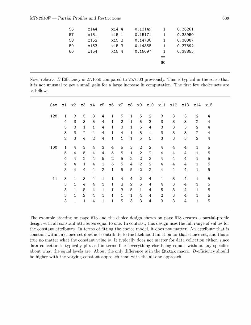
MR-2010F — Partial Profiles and Restrictions 639
56 x144 x14 4 0.13149 1 0.3626157 x151 x15 1 0.15171 1 0.3895058 x152 x15 2 0.14736 1 0.3838759 x153 x15 3 0.14358 1 0.3789260 x154 x15 4 0.15097 1 0.38855
==60
Now, relative D-Efficiency is 27.1650 compared to 25.7503 previously. This is typical in the sense thatit is not unusual to get a small gain for a large increase in computation. The first few choice sets areas follows:
Set x1 x2 x3 x4 x5 x6 x7 x8 x9 x10 x11 x12 x13 x14 x15
128 1 3 5 3 4 1 5 1 5 2 3 3 3 2 44 3 3 5 4 1 2 1 5 3 3 3 3 2 45 3 1 1 4 1 3 1 5 4 3 3 3 2 43 3 2 4 4 1 4 1 5 1 3 3 3 2 42 3 4 2 4 1 1 1 5 5 3 3 3 2 4
100 1 4 3 4 3 4 5 3 2 2 4 4 4 1 55 4 5 4 4 5 5 1 2 2 4 4 4 1 54 4 2 4 5 2 5 2 2 2 4 4 4 1 52 4 1 4 1 3 5 4 2 2 4 4 4 1 53 4 4 4 2 1 5 5 2 2 4 4 4 1 5
11 3 1 3 4 1 1 4 4 2 4 1 3 4 1 53 1 4 4 1 1 2 2 5 4 4 3 4 1 53 1 5 4 1 1 3 5 1 4 5 3 4 1 53 1 2 4 1 1 1 1 4 4 2 3 4 1 53 1 1 4 1 1 5 3 3 4 3 3 4 1 5
The example starting on page 613 and the choice design shown on page 618 creates a partial-profiledesign with all constant attributes equal to one. In contrast, this design uses the full range of values forthe constant attributes. In terms of fitting the choice model, it does not matter. An attribute that isconstant within a choice set does not contribute to the likelihood function for that choice set, and this istrue no matter what the constant value is. It typically does not matter for data collection either, sincedata collection is typically phrased in terms like “everything else being equal” without any specificsabout what the equal levels are. About the only difference is in the %MktEx macro. D-efficiency shouldbe higher with the varying-constant approach than with the all-one approach.

640 MR-2010F — Discrete Choice
Partial Profiles from Block Designs andOrthogonal Arrays
These next examples make optimal partial-profile designs from balanced incomplete block designs(BIBDs) and small orthogonal arrays (OAs). Before we get into partial profiles, let’s discuss BIBDsand review OAs.
Balanced Incomplete Block Designs
The following design is a BIBD:
Balanced Incomplete Block Design
x1 x2 x3 x4
10 4 16 116 13 14 1112 15 4 148 10 2 1313 9 1 154 6 13 57 5 15 105 12 8 169 14 5 23 5 11 17 13 3 122 15 3 1614 6 10 38 3 9 410 11 9 121 7 14 82 1 12 611 2 4 76 16 7 915 8 6 11
It consists of b = 20 rows or blocks. The design has k = 4 columns, so each block is of size four. Thedesign consists of the integers 1 to 16, so over the entire design, there are t = 16 attributes. Thedesign has a total of bk = 20× 4 = 80 elements. This design is balanced in the sense that each of thet = 16 attributes occurs exactly r = 5 times (rt = 5 × 16 = bk = 20 × 4 = 80). Furthermore, thet(t − 1)/2 = 16(16 − 1)/2 = bk(k − 1)/2 = 20 × 4(4 − 1)/2 = 120 pairs of attributes occur togetherin the same block exactly once. This is what makes this design a BIBD. The attribute by attributefrequencies are as follows:

MR-2010F — Partial Profiles from Block Designs and Orthogonal Arrays 641
Attribute by Attribute Frequencies
1 2 3 4 5 6 7 8 9 10 11 12 13 14 15 16
1 5 1 1 1 1 1 1 1 1 1 1 1 1 1 1 12 5 1 1 1 1 1 1 1 1 1 1 1 1 1 13 5 1 1 1 1 1 1 1 1 1 1 1 1 14 5 1 1 1 1 1 1 1 1 1 1 1 15 5 1 1 1 1 1 1 1 1 1 1 16 5 1 1 1 1 1 1 1 1 1 17 5 1 1 1 1 1 1 1 1 18 5 1 1 1 1 1 1 1 19 5 1 1 1 1 1 1 1
10 5 1 1 1 1 1 111 5 1 1 1 1 112 5 1 1 1 113 5 1 1 114 5 1 115 5 116 5
In the partial-profile context, this BIBD instructs us to create 20 blocks of choice sets. This BIBD canbe used for the situation where there are 16 attributes and 4 are varied at a time. In the first block,attributes 10, 4, 16, and 1 vary while the remaining attributes are held constant; in the second block,attributes 16, 13, 14, and 11 vary while the remaining attributes are held constant; and so on. Everyattribute appears in a block of choice sets with every other attribute and each attribute occurs exactlyas often as every other attribute. A BIBD is not an orthogonal array or ordinary factorial design likewe get out of the %MktEx macro, so we use a different tool, the %MktBIBD macro to find BIBDs. Formore information about BIBDs and how they relate to factorial designs see page 965. BIBDs only existfor specific and limited combinations of b, k, and t. We can run the %MktBSize macro to find sizes thatmeet necessary but not sufficient criteria for the existence of a BIBD as follows:
%mktbsize(b=20, nattrs=16, setsize=4)
This step reports the following, which shows that a BIBD might exist for this specification, but ofcourse we already knew that:
nt k b r Lambda TotalNumber of Set Number Attribute Pairwise SampleAttributes Size of Sets Frequency Frequencies Size
16 4 20 5 1 80

642 MR-2010F — Discrete Choice
More generally, we can run the %MktBSize macro with lists of parameters and get a list of thosecombinations of parameters that meet the necessary but not sufficient conditions for the existence of aBIBD. This list includes the design we just saw. The following step generates the list:
%mktbsize(nattrs=15 to 20, setsize=3 to t / 2, b=t to 30)
The results are as follows:
nt k b r Lambda TotalNumber of Set Number Attribute Pairwise SampleAttributes Size of Sets Frequency Frequencies Size
15 5 21 7 2 10515 7 15 7 3 10516 4 20 5 1 8016 6 16 6 2 9616 8 30 15 7 24019 9 19 9 4 171
There is no guarantee that %MktBIBD will find a BIBD for any specification, even when one is in factknown to exist. However, it usually does quite well in finding smaller BIBDS and in finding designs thatare close the rest of the time. When it cannot find a BIBD, it finds a design where each attribute occursas often as every other attribute or almost as often and each pair of attributes occurs together almostequally often. Furthermore, the %MktBIBD macro can find designs like this even when the parametersdo not meet the necessary criteria. For the purposes of making a partial-profile design, a block designwith almost equal frequencies is usually good enough. The following step shows how we found theBIBD shown in the beginning of this section:
%mktbibd(b=20, nattrs=16, setsize=4, seed=17)
The entire set of output from this macro is as follows:
Block Design Efficiency Criterion 100.0000Number of Attributes, t 16Set Size, k 4Number of Sets, b 20Attribute Frequency 5Pairwise Frequency 1Total Sample Size 80Positional Frequencies Optimized? Yes

MR-2010F — Partial Profiles from Block Designs and Orthogonal Arrays 643
Attribute by Attribute Frequencies
1 2 3 4 5 6 7 8 9 10 11 12 13 14 15 16
1 5 1 1 1 1 1 1 1 1 1 1 1 1 1 1 12 5 1 1 1 1 1 1 1 1 1 1 1 1 1 13 5 1 1 1 1 1 1 1 1 1 1 1 1 14 5 1 1 1 1 1 1 1 1 1 1 1 15 5 1 1 1 1 1 1 1 1 1 1 16 5 1 1 1 1 1 1 1 1 1 17 5 1 1 1 1 1 1 1 1 18 5 1 1 1 1 1 1 1 19 5 1 1 1 1 1 1 1
10 5 1 1 1 1 1 111 5 1 1 1 1 112 5 1 1 1 113 5 1 1 114 5 1 115 5 116 5
Attribute by Position Frequencies
1 2 3 4
1 1 1 1 22 2 1 1 13 1 1 2 14 1 1 2 15 1 2 1 16 1 2 1 17 2 1 1 18 2 1 1 19 1 1 2 110 2 1 1 111 1 1 1 212 1 1 1 213 1 2 1 114 1 1 2 115 1 2 1 116 1 1 1 2

644 MR-2010F — Discrete Choice
Balanced Incomplete Block Design
x1 x2 x3 x4
10 4 16 116 13 14 1112 15 4 148 10 2 1313 9 1 154 6 13 57 5 15 105 12 8 169 14 5 23 5 11 17 13 3 122 15 3 1614 6 10 38 3 9 410 11 9 121 7 14 82 1 12 611 2 4 76 16 7 915 8 6 11
The first part of the output consists of a “factoid” of miscellaneous statistics, parameters, and informa-tion. The efficiency criterion is 100, so a BIBD was found. Next, the parameters of the BIBD, t = 16,k = 4, and b = 20 are reported. The attribute frequency of 5 shows that each of the t = 16 attributesoccurs five times in the array. Each pair of attributes occurs once. The total sample size refers to thebk = 20 × 4 = 80 elements in the BIBD. In the final BIBD, the positional frequencies are optimized.This is shown in the attribute by position frequencies, which are discussed soon.
The factoid is followed by the attribute by attribute frequency matrix. We want to see a constantdiagonal and a constant upper triangular matrix above the diagonal, and that is what we get sincewe have a BIBD. The next matrix contains the attribute by position frequencies. We see that eachattribute occurs in each position either one or two times. It is impossible for the results to be constantin this BIBD. However, they are as close to constant as they possibly can be, and there are no zeros,threes, or greater values. Note though, that the attribute by position frequencies are not important tous in the partial-profile context. We could specify positer= to turn off the iterations that optimizethe positional frequencies to make the macro run faster for this problem. In this case, we get the sameBIBD, but with the values in a different order within row. The last matrix is the BIBD.

MR-2010F — Partial Profiles from Block Designs and Orthogonal Arrays 645
Orthogonal Arrays
An orthogonal array (OA) is a factorial design in which all estimable effects are uncorrelated. The%MktEx macro has an extensive catalog of orthogonal arrays. A sample of a small OA is as follows:
x1 x2 x3 x4 x5
1 1 1 1 11 2 2 2 22 1 2 1 22 2 1 2 13 1 1 2 23 2 2 1 14 1 2 2 14 2 1 1 2
This design is balanced—each of the four levels of x1 occurs exactly twice, and each of the two levelsof x2-x4 occurs exactly four times. This design is orthogonal—each of the eight pairs of levels of x1with x2-x5 occurs exactly once, and each of the four pairs of levels for each of the pairs of factors inx2-x5 occurs exactly twice. Hence this design is an OA. It can be created as follows:
%mktex(4 2**4, n=8)
proc print noobs; run;
80 Choice Sets, 16 Binary Attributes, Four Varying
In this example, we create a partial-profile design with t = 16 binary attributes and k = 4 varying atone time. We create 80 choice sets of two alternatives each. The resulting design is optimal under theassumption β = 0 (Anderson 2003). The following steps create and evaluate the design:
%mktbibd(b=20, nattrs=16, setsize=4, seed=17)
%mktex(4 2 ** 4, n=8, seed=306)
proc sort data=randomized out=randes(drop=x1);by x2 x1;run;
proc print noobs data=randes; run;
%mktppro(design=randes, ibd=bibd)

646 MR-2010F — Discrete Choice
%choiceff(data=chdes, /* candidate set of choice sets */init=chdes, /* initial design */initvars=x1-x6, /* factors in the initial design */model=class(x1-x16 / sta),/* model with stdz orthogonal coding */nsets=80, /* number of choice sets */nalts=2, /* number of alternatives */rscale= /* relative D-efficiency scale factor */%sysevalf(80 * 4 / 16), /* 4 of 16 attrs in 80 sets vary */beta=zero) /* assumed beta vector, Ho: b=0 */
proc print data=chdes(obs=12); id set; by set; run;
%mktdups(generic, data=best, factors=x1-x16, nalts=2)
The first step makes the BIBD as we saw in the previous step. It tells us which attributes to vary ineach choice set. The following design is a BIBD:
Balanced Incomplete Block Design
x1 x2 x3 x4
1 4 16 1016 13 14 1112 15 4 148 10 2 1313 9 1 154 6 13 510 5 15 75 12 8 169 14 5 23 5 11 17 13 3 1216 2 3 1514 6 10 38 3 9 49 11 12 101 7 14 82 1 12 611 4 2 76 16 7 915 8 6 11
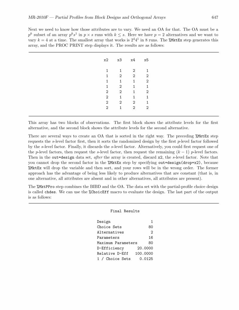
MR-2010F — Partial Profiles from Block Designs and Orthogonal Arrays 647
Next we need to know how those attributes are to vary. We need an OA for that. The OA must be apk subset of an array pks1 in p × s runs with k ≤ s. Here we have p = 2 alternatives and we want tovary k = 4 at a time. The smallest array that works is 2441 in 8 runs. The %MktEx step generates thisarray, and the PROC PRINT step displays it. The results are as follows:
x2 x3 x4 x5
1 1 2 11 2 2 21 1 1 21 2 1 12 2 1 22 1 1 12 2 2 12 1 2 2
This array has two blocks of observations. The first block shows the attribute levels for the firstalternative, and the second block shows the attribute levels for the second alternative.
There are several ways to create an OA that is sorted in the right way. The preceding %MktEx steprequests the s-level factor first, then it sorts the randomized design by the first p-level factor followedby the s-level factor. Finally, it discards the s-level factor. Alternatively, you could first request one ofthe p-level factors, then request the s-level factor, then request the remaining (k − 1) p-level factors.Then in the out=design data set, after the array is created, discard x2, the s-level factor. Note thatyou cannot drop the second factor in the %MktEx step by specifying out=design(drop=x2), because%MktEx will drop the variable and then sort, and your rows will be in the wrong order. The formerapproach has the advantage of being less likely to produce alternatives that are constant (that is, inone alternative, all attributes are absent and in other alternatives, all attributes are present).
The %MktPPro step combines the BIBD and the OA. The data set with the partial-profile choice designis called chdes. We can use the %ChoicEff macro to evaluate the design. The last part of the outputis as follows:
Final Results
Design 1Choice Sets 80Alternatives 2Parameters 16Maximum Parameters 80D-Efficiency 20.0000Relative D-Eff 100.00001 / Choice Sets 0.0125
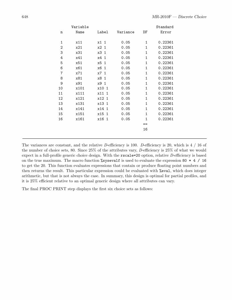
648 MR-2010F — Discrete Choice
Variable Standardn Name Label Variance DF Error
1 x11 x1 1 0.05 1 0.223612 x21 x2 1 0.05 1 0.223613 x31 x3 1 0.05 1 0.223614 x41 x4 1 0.05 1 0.223615 x51 x5 1 0.05 1 0.223616 x61 x6 1 0.05 1 0.223617 x71 x7 1 0.05 1 0.223618 x81 x8 1 0.05 1 0.223619 x91 x9 1 0.05 1 0.2236110 x101 x10 1 0.05 1 0.2236111 x111 x11 1 0.05 1 0.2236112 x121 x12 1 0.05 1 0.2236113 x131 x13 1 0.05 1 0.2236114 x141 x14 1 0.05 1 0.2236115 x151 x15 1 0.05 1 0.2236116 x161 x16 1 0.05 1 0.22361
==16
The variances are constant, and the relative D-efficiency is 100. D-efficiency is 20, which is 4 / 16 ofthe number of choice sets, 80. Since 25% of the attributes vary, D-efficiency is 25% of what we wouldexpect in a full-profile generic choice design. With the rscale=20 option, relative D-efficiency is basedon the true maximum. The macro function %sysevalf is used to evaluate the expression 80 * 4 / 16to get the 20. This function evaluates expressions that contain or produce floating point numbers andthen returns the result. This particular expression could be evaluated with %eval, which does integerarithmetic, but that is not always the case. In summary, this design is optimal for partial profiles, andit is 25% efficient relative to an optimal generic design where all attributes can vary.
The final PROC PRINT step displays the first six choice sets as follows:

MR-2010F — Partial Profiles from Block Designs and Orthogonal Arrays 649
Set x1 x2 x3 x4 x5 x6 x7 x8 x9 x10 x11 x12 x13 x14 x15 x16
1 1 1 1 1 1 1 1 1 1 1 1 1 1 1 1 22 1 1 2 1 1 1 1 1 2 1 1 1 1 1 1
2 1 1 1 2 1 1 1 1 1 2 1 1 1 1 1 22 1 1 1 1 1 1 1 1 1 1 1 1 1 1 1
3 1 1 1 1 1 1 1 1 1 2 1 1 1 1 1 12 1 1 2 1 1 1 1 1 1 1 1 1 1 1 2
4 1 1 1 2 1 1 1 1 1 1 1 1 1 1 1 12 1 1 1 1 1 1 1 1 2 1 1 1 1 1 2
5 1 1 1 1 1 1 1 1 1 1 1 1 1 2 1 11 1 1 1 1 1 1 1 1 1 2 1 2 1 1 2
6 1 1 1 1 1 1 1 1 1 1 2 1 2 2 1 11 1 1 1 1 1 1 1 1 1 1 1 1 1 1 2
There are a total of 80 choice sets, b = 20 blocks of size s = 4. The first four choice sets show the 8-runOA embedded in the partial-profile design in columns 1, 4, 10, and 16, as directed by the first row ofthe BIBD. The next four choice sets (only two are shown) show the same 8-run OA embedded in thepartial-profile design in columns 11, 13, 14, and 16, as directed by the second row of the BIBD.
We have already seen that the choice design is statistically optimal. However, it might not be optimalfrom a practical usage point of view. In every choice set, there is a pair of alternatives, one withthree attributes present and one with only one attribute present. This might not meet your needs (ormaybe it does). You always need to inspect your designs to see how well they work for your purposes.Statistical efficiency and optimality are just one part of the picture. With the OA 4124 in 8 runs,there is one other kind of OA that you can get by specifying other random number seeds, that alwaysproduces a choice set (one in each block of choice sets) where all four attributes are present in onealternative and none are present in the other alternative. This might be worse. This kind of problemis less likely to be an issue when you vary more than four attributes.
The output from the %MktDups macro is as follows:
Design: GenericFactors: x1-x16
x1 x2 x3 x4 x5 x6 x7 x8 x9 x10 x11 x12 x13 x14 x15 x16Sets w Dup Alts: 0Duplicate Sets: 0
There are no duplicates.

650 MR-2010F — Discrete Choice
80 Choice Sets, 16 Binary Attributes, Four Varying, Part 2
This example is identical to the previous example except that now b = 12 blocks are requested insteadof 20, resulting in 48 choice sets instead of 80. The following steps create the design:
%mktbibd(b=12, nattrs=16, setsize=4, seed=17)
%mktex(4 2 ** 4, n=8, seed=306)
proc sort data=randomized out=randes(drop=x1);by x2 x1;run;
%mktppro(ibd=bibd, design=randes)
%choiceff(data=chdes, /* candidate set of choice sets */init=chdes, /* initial design */initvars=x1-x6, /* factors in the initial design */model=class(x1-x16 / sta),/* model with stdz orthogonal coding */nsets=48, /* number of choice sets */nalts=2, /* number of alternatives */rscale= /* relative D-efficiency scale factor */%sysevalf(48 * 4 / 16), /* 4 of 16 attrs in 80 sets vary */beta=zero) /* assumed beta vector, Ho: b=0 */
%mktdups(generic, data=best, factors=x1-x16, nalts=2)
The first part of the output from the %MktBIBD macro is as follows:
Block Design Efficiency Criterion 98.0066Number of Attributes, t 16Set Size, k 4Number of Sets, b 12Average Attribute Frequency 3Average Pairwise Frequency 0.6Total Sample Size 48Positional Frequencies Optimized? Yes
We can see that our results, an unbalanced block design, is not a BIBD since the efficiency is not 100.The attribute by attribute frequencies are as follows:

MR-2010F — Partial Profiles from Block Designs and Orthogonal Arrays 651
Attribute by Attribute Frequencies
1 2 3 4 5 6 7 8 9 10 11 12 13 14 15 16
1 3 1 1 0 0 0 1 1 0 1 1 1 1 0 0 12 3 0 0 1 1 0 0 0 1 0 1 1 1 1 13 3 1 1 1 1 1 0 0 0 1 0 0 1 14 3 1 0 1 0 1 1 0 1 1 1 0 15 3 1 0 1 0 1 1 1 0 1 0 06 3 1 1 1 1 0 0 1 0 1 07 3 0 0 1 1 0 1 1 1 08 3 1 0 1 0 1 1 0 19 3 1 1 1 1 0 1 1
10 3 1 0 0 0 0 111 3 1 0 1 1 012 3 1 0 1 013 3 1 0 014 3 1 115 3 116 3
Each attribute occurs exactly 3 times, but each pair of attributes does not occur equally often. With20 blocks, each pair occurred exactly once, so with fewer blocks, the best we can do is some zeros andsome ones. The same is true for the attribute by position frequencies, which are as follows:
Attribute by Position Frequencies
1 2 3 4
1 1 1 1 02 1 0 1 13 1 1 1 04 1 0 1 15 1 1 1 06 0 1 1 17 1 1 0 18 1 1 0 19 1 0 1 110 1 0 1 111 1 1 1 012 0 1 1 113 0 1 1 114 0 1 1 115 1 1 0 1

652 MR-2010F — Discrete Choice
The unbalanced block design is as follows:
Design
x1 x2 x3 x4
9 11 12 1515 7 3 62 15 14 167 1 11 108 13 6 93 5 4 1216 3 1 810 16 9 41 12 2 134 14 13 711 8 5 145 6 10 2
The last part of the output from the %ChoicEff macro’s evaluation of the design is as follows:
Final Results
Design 1Choice Sets 48Alternatives 2Parameters 16Maximum Parameters 48D-Efficiency 12.0000Relative D-Eff 100.0000D-Error 0.08331 / Choice Sets 0.0208

MR-2010F — Partial Profiles from Block Designs and Orthogonal Arrays 653
Variable Standardn Name Label Variance DF Error
1 x11 x1 1 0.083333 1 0.288682 x21 x2 1 0.083333 1 0.288683 x31 x3 1 0.083333 1 0.288684 x41 x4 1 0.083333 1 0.288685 x51 x5 1 0.083333 1 0.288686 x61 x6 1 0.083333 1 0.288687 x71 x7 1 0.083333 1 0.288688 x81 x8 1 0.083333 1 0.288689 x91 x9 1 0.083333 1 0.2886810 x101 x10 1 0.083333 1 0.2886811 x111 x11 1 0.083333 1 0.2886812 x121 x12 1 0.083333 1 0.2886813 x131 x13 1 0.083333 1 0.2886814 x141 x14 1 0.083333 1 0.2886815 x151 x15 1 0.083333 1 0.2886816 x161 x16 1 0.083333 1 0.28868
==16
The relative D-efficiency is 100% corresponding to 4 / 16 of 48 choice sets. This design is optimal! Itis optimal even though our block design is not balanced. We might not have used a real BIBD, but wedid use a real OA, and that is what is critical to achieve optimality. It is optimal for a partial-profiledesign in 48 choices sets even though it provides less information than a design optimized for a largernumber of choice sets such as 80.
The output from the %MktDups macro is as follows:
Design: GenericFactors: x1-x16
x1 x2 x3 x4 x5 x6 x7 x8 x9 x10 x11 x12 x13 x14 x15 x16Sets w Dup Alts: 0Duplicate Sets: 0
There are no duplicates.
Note again, however, that while this design is statistically optimal, it might not be optimal from apractical usage point of view. Besides the problems with the imbalance in the number of attributesshown in each alternative, now every attribute is no longer paired with every other attribute. Theseare issues you need to think about when you evaluate your designs.

654 MR-2010F — Discrete Choice
80 Choice Sets, 16 Binary Attributes, Four Varying, Part 3
This example is identical to the previous example except that now b = 8 blocks are requested insteadof 12 or 20, resulting in 32 choice sets instead of 48 or 80. The following steps create and evaluate thedesign:
%mktbibd(b=8, nattrs=16, setsize=4, seed=17)
%mktex(4 2 ** 4, n=8, seed=306)
proc sort data=randomized out=randes(drop=x1);by x2 x1;run;
%mktppro(ibd=bibd, design=randes)
%choiceff(data=chdes, /* candidate set of choice sets */init=chdes, /* initial design */initvars=x1-x6, /* factors in the initial design */model=class(x1-x16 / sta),/* model with stdz orthogonal coding */nsets=32, /* number of choice sets */nalts=2, /* number of alternatives */rscale= /* relative D-efficiency scale factor */%sysevalf(32 * 4 / 16), /* 4 of 16 attrs in 32 sets vary */beta=zero) /* assumed beta vector, Ho: b=0 */
%mktdups(generic, data=best, factors=x1-x16, nalts=2)
The attribute by attribute frequencies are as follows:
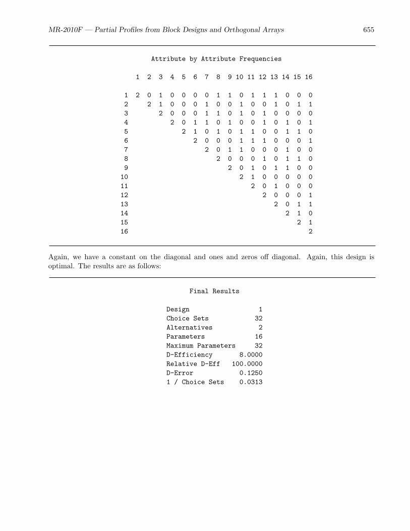
MR-2010F — Partial Profiles from Block Designs and Orthogonal Arrays 655
Attribute by Attribute Frequencies
1 2 3 4 5 6 7 8 9 10 11 12 13 14 15 16
1 2 0 1 0 0 0 0 1 1 0 1 1 1 0 0 02 2 1 0 0 0 1 0 0 1 0 0 1 0 1 13 2 0 0 0 1 1 0 1 0 1 0 0 0 04 2 0 1 1 0 1 0 0 1 0 1 0 15 2 1 0 1 0 1 1 0 0 1 1 06 2 0 0 0 1 1 1 0 0 0 17 2 0 1 1 0 0 0 1 0 08 2 0 0 0 1 0 1 1 09 2 0 1 0 1 1 0 0
10 2 1 0 0 0 0 011 2 0 1 0 0 012 2 0 0 0 113 2 0 1 114 2 1 015 2 116 2
Again, we have a constant on the diagonal and ones and zeros off diagonal. Again, this design isoptimal. The results are as follows:
Final Results
Design 1Choice Sets 32Alternatives 2Parameters 16Maximum Parameters 32D-Efficiency 8.0000Relative D-Eff 100.0000D-Error 0.12501 / Choice Sets 0.0313

656 MR-2010F — Discrete Choice
Variable Standardn Name Label Variance DF Error
1 x11 x1 1 0.125 1 0.353552 x21 x2 1 0.125 1 0.353553 x31 x3 1 0.125 1 0.353554 x41 x4 1 0.125 1 0.353555 x51 x5 1 0.125 1 0.353556 x61 x6 1 0.125 1 0.353557 x71 x7 1 0.125 1 0.353558 x81 x8 1 0.125 1 0.353559 x91 x9 1 0.125 1 0.3535510 x101 x10 1 0.125 1 0.3535511 x111 x11 1 0.125 1 0.3535512 x121 x12 1 0.125 1 0.3535513 x131 x13 1 0.125 1 0.3535514 x141 x14 1 0.125 1 0.3535515 x151 x15 1 0.125 1 0.3535516 x161 x16 1 0.125 1 0.35355
==16
It is optimal for a partial-profile design in 32 choices sets even though it provides less information thandesigns optimized for a larger number of choice sets such as 48 or 80.
The output from the %MktDups macro is as follows:
Design: GenericFactors: x1-x16
x1 x2 x3 x4 x5 x6 x7 x8 x9 x10 x11 x12 x13 x14 x15 x16Sets w Dup Alts: 0Duplicate Sets: 0
There are no duplicates.
80 Choice Sets, 16 Binary Attributes, Four Varying, Part 4
This example is identical to the previous example except that now b = 7 blocks are requested insteadof a multiple of 4. The following steps create the design:
%mktbibd(b=7, nattrs=16, setsize=4, seed=17)
%mktex(4 2 ** 4, n=8, seed=306)
proc sort data=randomized out=randes(drop=x1);by x2 x1;run;

MR-2010F — Partial Profiles from Block Designs and Orthogonal Arrays 657
%mktppro(ibd=bibd, design=randes)
%choiceff(data=chdes, /* candidate set of choice sets */init=chdes, /* initial design */initvars=x1-x6, /* factors in the initial design */model=class(x1-x16 / sta),/* model with stdz orthogonal coding */nsets=28, /* number of choice sets */nalts=2, /* number of alternatives */rscale= /* relative D-efficiency scale factor */%sysevalf(28 * 4 / 16), /* 4 of 16 attrs in 28 sets vary */beta=zero) /* assumed beta vector, Ho: b=0 */
%mktdups(generic, data=best, factors=x1-x16, nalts=2)
The attribute by attribute frequencies are as follows:
Attribute by Attribute Frequencies
1 2 3 4 5 6 7 8 9 10 11 12 13 14 15 16
1 2 0 0 1 0 0 0 0 1 0 1 1 1 0 1 02 2 0 0 0 0 1 1 0 1 0 0 1 0 1 13 2 0 0 1 1 0 1 0 0 1 0 1 0 14 1 0 0 0 0 0 0 0 1 0 0 1 05 1 1 0 0 0 1 1 0 0 0 0 06 2 0 0 0 1 1 1 0 0 0 17 2 0 1 1 0 0 0 1 1 08 1 0 0 0 0 1 0 0 19 2 0 1 0 1 1 0 0
10 2 1 0 0 0 1 011 2 0 1 0 0 012 2 0 0 1 113 2 0 0 114 1 0 015 2 016 2
The 16 attributes cannot be equally distributed across the 7×4 entries in the incomplete block design,so the diagonal has nonconstant frequencies. The evaluation is as follows:

658 MR-2010F — Discrete Choice
Final Results
Design 1Choice Sets 28Alternatives 2Parameters 16Maximum Parameters 28D-Efficiency 6.7272Relative D-Eff 96.1024D-Error 0.14871 / Choice Sets 0.0357
Variable Standardn Name Label Variance DF Error
1 x11 x1 1 0.125 1 0.353552 x21 x2 1 0.125 1 0.353553 x31 x3 1 0.125 1 0.353554 x41 x4 1 0.250 1 0.500005 x51 x5 1 0.250 1 0.500006 x61 x6 1 0.125 1 0.353557 x71 x7 1 0.125 1 0.353558 x81 x8 1 0.250 1 0.500009 x91 x9 1 0.125 1 0.3535510 x101 x10 1 0.125 1 0.3535511 x111 x11 1 0.125 1 0.3535512 x121 x12 1 0.125 1 0.3535513 x131 x13 1 0.125 1 0.3535514 x141 x14 1 0.250 1 0.5000015 x151 x15 1 0.125 1 0.3535516 x161 x16 1 0.125 1 0.35355
==16
The design does not have a relative D-efficiency of 100%, so it is not optimal relative to a hypothetical,optimal partial-profile design. With seven blocks, or any b not a multiple of 4, the kind of combinatorialoptimality we saw previously is not possible.
The output from the %MktDups macro is as follows:
Design: GenericFactors: x1-x16
x1 x2 x3 x4 x5 x6 x7 x8 x9 x10 x11 x12 x13 x14 x15 x16Sets w Dup Alts: 0Duplicate Sets: 0

MR-2010F — Partial Profiles from Block Designs and Orthogonal Arrays 659
There are no duplicates.
Partial Profiles, the General Combinatorial Approach
In the previous sections, we saw several examples of using the %MktBIBD macro to make BIBDs, the%MktEx macro to make OAs, the %MktPPro macro to combine them into a partial-profile design, andthe %ChoicEff macro to evaluate the design. Next an ad hoc wrapper macro that combines them intoa single macro for making partial-profile designs based on this combinatorial structure is shown. Itworks for attr attributes and lev-level factors, with vary varying, and maxv × lev rows in each of the bblocks of choice sets. The macro is as follows:
%macro pp( /*--------------------------------------*/lev=, /* levels */nattrs=, /* total attributes */setsize=, /* number of attributes that vary */maxv=, /* max number of attrs that can vary */b=, /* number of blocks */seed=); /* random number seed */
/*--------------------------------------*/
%let sets = %sysevalf(&b * &maxv);%put NOTE: nattrs=&nattrs, setsize=&setsize, sets=&sets, b=&b..;
%mktbibd(b=&b, nattrs=&nattrs, setsize=&setsize, seed=&seed, positer=0)
%mktex(&maxv &lev ** &setsize, n=&lev * &maxv)
proc sort data=randomized out=randes(drop=x1);by x2 x1;run;
%mktppro(ibd=bibd, design=randes)
%choiceff(data=chdes, /* candidate set of choice sets */init=chdes, /* initial design */initvars=x1-x&nattrs, /* factors in the initial design */intiter=0, /* evaluate without internal iterations */model=class(x1-x&nattrs / sta),/* model with stdz orthog coding */nsets=&sets, /* number of choice sets */nalts=&lev, /* number of alternatives */rscale= /* relative D-efficiency scale factor */%sysevalf(&sets * &setsize / &nattrs),beta=zero) /* assumed beta vector, Ho: b=0 */
proc print data=chdes; by set; id set; var x:; run;
%mktdups(generic, data=best, factors=x1-x&nattrs, nalts=&lev)%mend;

660 MR-2010F — Discrete Choice
The next steps create 25 examples of partial-profile designs. Thousands more could be made. You canuse any positive integer < 231− 1 for a seed.∗ Note that some are subject to problems with duplicates.The following steps create the designs:
%pp(lev = 2, nattrs = 16, setsize = 4, maxv = 4, b = 20, seed = 17)%pp(lev = 4, nattrs = 16, setsize = 4, maxv = 4, b = 20, seed = 93)%pp(lev = 2, nattrs = 16, setsize = 8, maxv = 8, b = 30, seed = 109)%pp(lev = 3, nattrs = 13, setsize = 6, maxv = 6, b = 26, seed = 114)%pp(lev = 2, nattrs = 23, setsize = 12, maxv = 12, b = 23, seed = 121)%pp(lev = 5, nattrs = 11, setsize = 5, maxv = 5, b = 11, seed = 145)%pp(lev = 3, nattrs = 19, setsize = 9, maxv = 9, b = 19, seed = 151)%pp(lev = 2, nattrs = 22, setsize = 7, maxv = 16, b = 22, seed = 205)%pp(lev = 4, nattrs = 13, setsize = 3, maxv = 8, b = 26, seed = 238)%pp(lev = 3, nattrs = 21, setsize = 5, maxv = 12, b = 21, seed = 289)%pp(lev = 2, nattrs = 22, setsize = 8, maxv = 20, b = 11, seed = 292)%pp(lev = 3, nattrs = 25, setsize = 9, maxv = 15, b = 25, seed = 306)%pp(lev = 4, nattrs = 21, setsize = 5, maxv = 12, b = 21, seed = 350)%pp(lev = 7, nattrs = 15, setsize = 7, maxv = 7, b = 15, seed = 368)%pp(lev = 5, nattrs = 16, setsize = 10, maxv = 10, b = 16, seed = 377)%pp(lev = 4, nattrs = 16, setsize = 8, maxv = 16, b = 10, seed = 382)%pp(lev = 8, nattrs = 15, setsize = 8, maxv = 8, b = 15, seed = 396)%pp(lev = 2, nattrs = 8, setsize = 2, maxv = 28, b = 28, seed = 420)%pp(lev = 5, nattrs = 7, setsize = 6, maxv = 15, b = 7, seed = 424)%pp(lev = 4, nattrs = 11, setsize = 6, maxv = 20, b = 11, seed = 448)%pp(lev = 3, nattrs = 45, setsize = 12, maxv = 27, b = 45, seed = 462)%pp(lev = 9, nattrs = 16, setsize = 4, maxv = 9, b = 20, seed = 472)%pp(lev = 3, nattrs = 15, setsize = 5, maxv = 30, b = 21, seed = 495)%pp(lev = 7, nattrs = 9, setsize = 3, maxv = 14, b = 12, seed = 513)%pp(lev = 5, nattrs = 13, setsize = 4, maxv = 20, b = 13, seed = 522)
It is instructive to see how these parameters are set, particularly maxv= and rep parameters. In thefirst example, there are 16 two-level attributes, and four vary at a time. This corresponds to a BIBDwith t = 14 and k = 4. We can run the %MktBSize macro with these specifications as follows:
%mktbsize(nattrs=16, setsize=4)
We see that a BIBD is available with each attribute appearing r = 5 times. This is the rep= parameterin the ad hoc macro. Remember though, that we do not need a BIBD in order to make good partial-profile designs. We can use other specifications as well, as long as there is an OA that works with ourblock design. We can find all OAs pks1 in p× s runs with k ≤ s as follows:
∗These are selected from some particularly interesting OA sections.
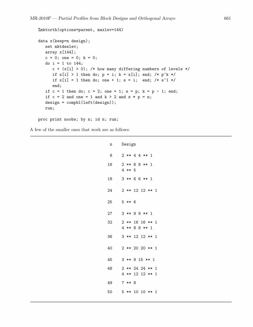
MR-2010F — Partial Profiles from Block Designs and Orthogonal Arrays 661
%mktorth(options=parent, maxlev=144)
data x(keep=n design);set mktdeslev;array x[144];c = 0; one = 0; k = 0;do i = 1 to 144;
c + (x[i] > 0); /* how many differing numbers of levels */if x[i] > 1 then do; p = i; k = x[i]; end; /* p^k */if x[i] = 1 then do; one + 1; s = i; end; /* s^1 */end;
if c = 1 then do; c = 2; one = 1; s = p; k = p - 1; end;if c = 2 and one = 1 and k > 2 and s * p = n;design = compbl(left(design));run;
proc print noobs; by n; id n; run;
A few of the smaller ones that work are as follows:
n Design
8 2 ** 4 4 ** 1
16 2 ** 8 8 ** 14 ** 5
18 3 ** 6 6 ** 1
24 2 ** 12 12 ** 1
25 5 ** 6
27 3 ** 9 9 ** 1
32 2 ** 16 16 ** 14 ** 8 8 ** 1
36 3 ** 12 12 ** 1
40 2 ** 20 20 ** 1
45 3 ** 9 15 ** 1
48 2 ** 24 24 ** 14 ** 12 12 ** 1
49 7 ** 8
50 5 ** 10 10 ** 1

662 MR-2010F — Discrete Choice
The first example used 2441 in 8 runs (2ks1 or 2setsizemaxv1). Note that you can always select a subsetof the available columns to vary (vary < k), and many of the examples do precisely that.
Efficient but Nonoptimal Partial Profiles
We can use the same methods to make efficient but nonoptimal partial-profile designs. With 12attributes, six varying, and six-level factors, an OA is not possible in 36 runs. Furthermore, with 12blocks of choice sets and 12 attributes and six varying, a BIBD is not possible either. Still, we can usean efficient factorial design and an unbalanced block design to make a partial-profile design as follows:
%mktbibd(b=12, nattrs=12, setsize=6, seed=93, positer=)
%mktex(6 ** 7, n=36, seed=238)
proc sort data=randomized out=randes(drop=x1);by x2 x1;run;
%mktppro(ibd=bibd, design=randes)
%choiceff(data=chdes, /* candidate set of choice sets */init=chdes, /* initial design */initvars=x1-x12, /* factors in the initial design */intiter=0, /* evaluate without internal iterations */model=class(x1-x12 / sta),/* model with stdz orthogonal coding */nsets=72, /* number of choice sets */nalts=6, /* number of alternatives */rscale= /* relative D-efficiency scale factor */%sysevalf(72 * 6 / 12), /* 6 of 12 attrs in 72 sets vary */beta=zero) /* assumed beta vector, Ho: b=0 */
proc print; by set; id set; var x1-x12; run;
%mktdups(generic, data=best, factors=x1-x12, nalts=6)

MR-2010F — Conclusions 663
Conclusions
This very long chapter has several purposes. It provides an introduction to the multinomial logit modelused in choice modeling, it discusses linear model designs created by the %MktEx macro and their use inchoice modeling, and it discusses using the %ChoicEff macro to find and evaluate designs. These twomacros, along with all of the other macros, provide powerful tools for designing choice experiments ina variety of ways. Numerous other macros and techniques are discussed as well.