discrete chirp-fourier transform and its application to ...xxia/dcft.pdf · discrete chirp-fourier...

3122 IEEE TRANSACTIONS ON SIGNAL PROCESSING, VOL. 48, NO. 11, NOVEMBER 2000

Discrete Chirp-Fourier Transform and Its Applicationto Chirp Rate Estimation

Xiang-Gen Xia, Senior Member, IEEE

Abstract—The discrete Fourier transform (DFT) has foundtremendous applications in almost all fields, mainly because it canbe used to match the multiple frequencies of a stationary signalwith multiple harmonics. In many applications, wideband andnonstationary signals, however, often occur. One of the typicalexamples of such signals is chirp-type signals that are usuallyencountered in radar signal processing, such as synthetic apertureradar (SAR) and inverse SAR imaging. Due to the motion of atarget, the radar return signals are usually chirps, and their chirprates include the information about the target, such as the locationand the velocity.

In this paper, we study discrete chirp-Fourier transform(DCFT), which is analogous to the DFT. Besides the multiplefrequency matching similar to the DFT, the DCFT can be usedto match the multiple chirp rates in a chirp-type signal withmultiple chirp components. We show that when the signal length

is prime, the magnitudes of all the sidelobes of the DCFTof a quadratic chirp signal are 1, whereas the magnitude of themainlobe of the DCFT is . With this result, an upper boundfor the number of the detectable chirp components using theDCFT is provided in terms of signal length and signal and noisepowers. We also show that the -point DCFT performs optimallywhen is a prime.

Index Terms—Chirp-Fourier transform, chirp rate estimation,chirps.

I. INTRODUCTION

T HE DISCRETE Fourier transform (DFT) has been appliedin almost all fields. The main reason is because the DFT

matches the frequencies in a signal of multiple harmonics. Inother words, if a signal has only several harmonics, the DFTof this signal has and only has peaks at the frequencies of thesignal harmonics, and the peak values correspond to the signalpowers at the corresponding harmonic frequencies. Therefore,the DFT can be used to estimate the Fourier spectrum of a signal,which is known asspectrum estimation, that plays an impor-tant role in digital signal processing applications. However, inorder to have the DFT work well, a signal has to be stationary.Although the stationarity assumption applies in many applica-tions, nonstationary signals often occur in some real applica-tions. Examples of nonstationary signals are chirp-type signals

Manuscript received May 12, 1999; revised July 16, 2000. This work wassupported in part by the Office of Naval Research Young Investigator Programunder Grant N00014-98-1-0644, the Air Force Office of Scientific Research(AFOSR) under Grant F49620-00-1-0086, and the National Science Founda-tion (NSF) CAREER under Grant MIP-9703377. The associate editor coordi-nating the review of this paper and approving it for publication was Prof. GregoriVazquez.

The author is with Department of Electrical and Computer Engineering, Uni-versity of Delaware, Newark, DE 19716 USA (e-mail: [email protected]).

Publisher Item Identifier S 1053-587X(00)09308-9.

that are encountered in radar signal processing, such as in syn-thetic aperture radar (SAR) and inverse SAR (ISAR) imaging;see, for example, [1]. In SAR imaging, when targets are moving,the radar return signals are chirps, in particularquadratic chirps,when the velocities of the moving targets are constant. In ISARimaging, when targets have maneuvering motions, the radar re-turn signals are also chirps. It is well known in the SAR andISAR literature that the direct DFT applications to the radar re-turn signals will smear the SAR or ISAR images of the targets.Furthermore, the chirp rates in the radar return signals includethe important information about the moving targets, such as thevelocities and the location parameters of the moving targets inSAR imaging. Therefore, the estimation of the chirp rates arecritically important in these applications.

For chirp-type signals, besides frequencies of multiple har-monics, there are chirp rates of multiple chirps, and the DFTcan be used only to match the multiple frequencies, but the mul-tiple chirps, in this case, may even reduce the resolution of thefrequency matching. The question of interest in this paper is togeneralize the DFT and its properties todiscrete chirp-Fouriertransform(DCFT) and corresponding properties, which is usednot only to match the multiple frequencies but to match the mul-tiple chirp rates, simultaneously as well.

It should be noticed that there has been much researchon chirp-type signals and their chirp rate estimations, suchas high-order ambiguity functions [2]–[4], adaptive chirplettransforms [10], [11], and other polynomial phase signalestimations [7]–[9]. In addition, the chirp-transform wasproposed in [12] for the efficient DFT implementation but notfor chirp rate estimation. However, the goal of this paper isfor chirp signal analysis and is, therefore, different. We firstgeneralize the DFT to the DCFT and then study the propertiesof the DCFT analogous to the DFT. In particular, we showthat when signal length is a prime, the magnitudes of allthe sidelobes (i.e., when the chirp rate is not matched) of theDCFT of a single quadratic chirp signal without noise are 1,whereas the magnitude of the mainlobe (i.e., when the chirprate and the harmonic frequency are both matched) of theDCFT is . The mainlobe and sidelobe magnitude ratio inthis case is , which is shown to be optimal for a givenlength . In other words, the DCFT performs optimally in thematching of the constant frequency and the chirp rate when thesignal length is a prime. When the chirp rate is preciselymatched, the DCFT is reduced to the DFT. Notice that for anysignal length , the magnitudes of all the sidelobes of the DFTof a single harmonic signal without noise are 0, whereas themagnitude of the mainlobe of the DFT is . The mainlobeand sidelobe magnitude ratio in this case is infinity, which tells

1053–587X/00$10.00 © 2000 IEEE

Authorized licensed use limited to: IEEE Xplore. Downloaded on November 26, 2008 at 14:46 from IEEE Xplore. Restrictions apply.

XIA: DISCRETE CHIRP-FOURIER TRANSFORM AND ITS APPLICATION TO CHIRP RATE ESTIMATION 3123

us that many different harmonics can be estimated using theDFT when there is no noise. In general, unlike the DFT forthe harmonic estimation, less than many different chirpscan be estimated using the DCFT. This paper is focused onquadratic chirps that are common in radar applications.

This paper is organized as follows. In Section II, we intro-duce the DCFT and study its basic properties for single com-ponent chirp signals. In Section III, we study the properties ofthe DCFT for multiple component chirp signals. We present anupper bound for the number of the components such that theyare detectable using the DCFT. In Section IV, we study its con-nection with the analog chirp-Fourier transform. In Section V,we present some numerical examples.

II. DISCRETECHIRP-FOURIER TRANSFORM AND ITS BASIC

PROPERTIES FORSINGLE COMPONENTCHIRP SIGNALS

Before going to the DCFT, let us first briefly recall the DFT.For a signal with length , its -point DFT is defined as

(2.1)

where . The key properties of the DFTare based on the following elementary identity

(2.2)

where takes 1 when and 0 otherwise. The identity(2.2) implies that if is a single harmonic, i.e.,

for some integer with , then its DFT matchesthe frequency perfectly, i.e.,

(2.3)

Based on this property, when has harmonics with ,i.e.,

where for , its DFT matches these frequenciesperfectly, i.e.,

(2.4)

where the peaks in the DFT domain are shown at all, and thecorresponding peak values are for .

We now introduce thediscrete chirp-Fourier transform(DCFT). Let , be a signal of length .Its -point DCFT is defined as

(2.5)

where represents the constant frequencies andrepresent thechirp rates. From the above DCFT, one can see that for eachfixed , is the DFT of the signal .When , the DCFT is the same as the DFT. Therefore, theinverse DCFT (IDCFT) is

(2.6)

where is an arbitrarily fixed integer. The above connection be-tween the DCFT and the DFT also suggests a fast algorithm tocompute the DCFT, i.e., for each, the FFT may be used to com-pute , . The computational complexitywith this approach is, thus, .

As a remark, the above chirp-Fourier transform is relatedto the fractional Fourier transform (FRFT), where the rotationangle is related to the variablein the DCFT. For more aboutFRFT, see, for example, [13]–[17].

The above DCFT definition is not surprising to see by fol-lowing the DFT definition. What is more interesting is its prop-erties. Can it be used to match the chirp rates and the constantfrequencies simultaneously? If so, how many of the chirp com-ponents can be matched simultaneously? Similar to the previousDFT study, let us first consider a single chirp signal

(2.7)

where and are two integers with , .When and in the DCFT (2.5) precisely match the aboveand , we have

which is called themainlobeof the DCFT . The ques-tion of interest here is what happens when the chirp rateandthe constant frequencydo not match and , i.e., what thesidelobesof the DCFT are. Is there a similar property for theDCFT as (2.3) for the DFT? To study these questions, we firsthave the following lemma.

Lemma 1: When is a prime, we have the following iden-tity: For ,

and

but

(2.8)



Proof: Let

Then, for

(2.9)

where , and the new range of in the summationin Step 1 is from the periodicity of in terms of the integervariable for any integer . When is a prime, for

, and is a multiple of if and onlyif is a multiple of , i.e., . Thus

for

Therefore, when . When , isreduced to (2.2). This proves the lemma.

From the second half of the above proof, one can see whyneeds to be prime in order for the second equality in (2.8)

to hold. From this lemma, we immediately have the followingresult.

Theorem 1: Let be a single chirp

(2.10)

for some integers and with , . If thelength is a prime, then its DCFT magnitude has the followingform:

when andwhenwhen but

(2.11)

This result tells us that for a single quadratic chirp, the peak orthe mainlobe of its DCFT has value and appears atin the DCFT domain and that the sidelobes are not above 1. Inother words, the DCFT of a single quadratic chirp matches itschirp rate and its constant frequency simultaneously. Sur-prisingly, one can see that all the magnitudes of the sidelobes,unless the chirp rate is matched, are all the same, which is 1.

In chirp rate and constant frequency estimation, the smallerthe sidelobe magnitudes of the DCFT, the better the perfor-mance of the estimation. When is a prime, from (2.11), themaximal sidelobe magnitude of the DCFT is 1, i.e.,

when is a prime (2.12)

One might want to ask what will happen whenis not a prime.The following result tells us that the maximal sidelobe magni-tude is the minimal when is a prime, i.e., the -point DCFTperforms the best when is a prime in the estimation of chirprates and constant frequencies. This will be also seen from thenumerical simulations in Section V.

Theorem 2: Let be the same as in Theorem 1, i.e., havethe form in (2.10). If the length is not a prime, then the max-imal sidelobe magnitude of the DCFT satisfies

(2.13)

Proof: To prove (2.13), it is enough to prove that whenis not a prime, the following inequality holds:

(2.14)

where is defined in the Proof of Lemma 1. Assumeis not a prime, and let with and .

Case i): Both and are odd. In this case, letand . Then, by (2.9)

Since is odd, is a multiple of if and only if is amultiple of . Thus

if is not a multiple of

Therefore, by setting , we have

Case ii): One of and is even. Without loss of gener-ality, we may assume . Let . In this case,

. Thus, by (2.9)



Notice that is always even, which implies. Therefore

By combining Cases i) and ii), (2.14) is proved.By this result, in what follows, we only consider prime.

The above results are based on the assumption that bothandin (2.10) are integers. In practice, these two parameters may

not be precisely integers. Next, we want to briefly discuss theDCFT performance when they are not integers but are close tointegers. The reason why we only consider the case whenand

are close to integers is because of the following argument.Let us consider an analog chirp signal

(2.15)

and consider the sampling . Then, the sampled chirpbecomes

(2.16)

where and . There-fore, when is large enough (i.e., the sampling rate is fastenough), there exist integersand such that

and (2.17)

This implies that the real chirp rate is and thatthe real constant frequency is when integersand are estimated. It also tells us that for a practical chirpsignal in (2.15), we only need to consider the discretechirp signal in (2.16) with parameters and close tointegers.

We now consider a discrete chirp signal

(2.18)

where

and (2.19)

where and are two integers with , , and ,and are two positive numbers. By using the Taylor expansionof in terms of , it is not hard to see that

(2.20)

Thus, for

(2.21)

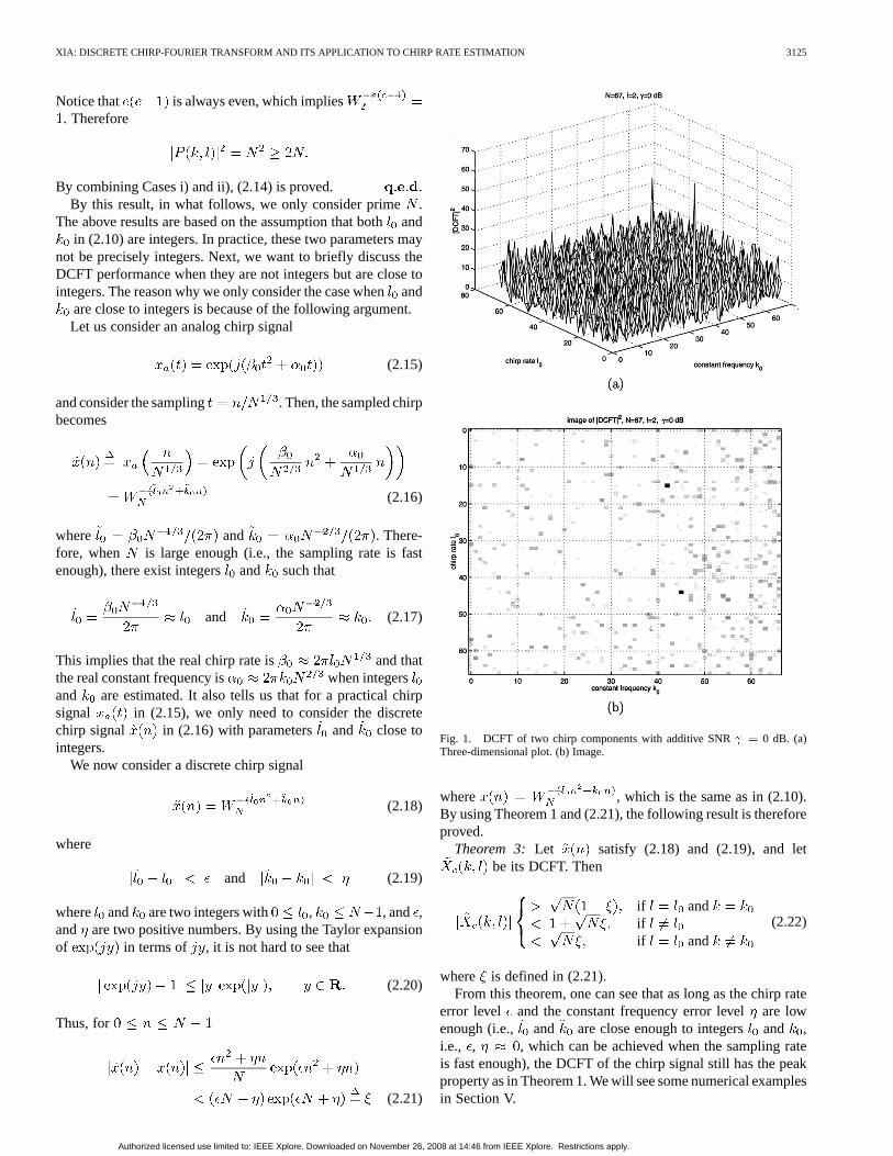
Fig. 1. DCFT of two chirp components with additive SNR = 0 dB. (a)Three-dimensional plot. (b) Image.

where , which is the same as in (2.10).By using Theorem 1 and (2.21), the following result is thereforeproved.

Theorem 3: Let satisfy (2.18) and (2.19), and letbe its DCFT. Then

if andifif and

(2.22)

where is defined in (2.21).From this theorem, one can see that as long as the chirp rate

error level and the constant frequency error levelare lowenough (i.e., and are close enough to integersand ,i.e., , , which can be achieved when the sampling rateis fast enough), the DCFT of the chirp signal still has the peakproperty as in Theorem 1. We will see some numerical examplesin Section V.



Fig. 2. DCFT of two chirp components with additive SNR = 6 dB. (a)Three-dimensional plot. (b) Image.

III. DCFT PROPERTIES FORMULTIPLE COMPONENTCHIRP

SIGNALS

We next consider a multiple component chirp signal ofthe form

(3.1)

where is an additive i.i.d. noise with mean 0 and variance, is the signal power of theth chirp component,

and for . For , let

(3.2)

Then, the DCFT of is

Fig. 3. DCFT of three chirp components with additive SNR = 0 dB. (a)Three-dimensional plot. (b) Image.

where is the DCFT of theth chirp component ,and is the DCFT of noise . From the study in Sec-tion II, we know that each has a peak at withpeak value , and the maximal off peak value is .What we are interested in here is whether there is a peak of

at each , . If there is a peak at, then a chirp component with constant frequencyand

chirp rate is detected. To study this question, let us calculatethe mean magnitude of . We first calculate the mean

at . For

(3.3)



Fig. 4. DCFT of three chirp components with additive SNR = 6 dB. (a)Three-dimensional plot. (b) Image.

where the inequality in Step 1 is becausefrom the Schwarz inequality with respect

to the expectation . Thus, to estimate the lower bound of themean magnitude , we need to estimate the meanpower of the DCFT of the noise . Since for any fixed ,

is the DFT of , the energy of interms of the frequency variable is the same as the one of

, i.e., the one of . This proves

(3.4)

Therefore, for by (3.3) and (3.4), we have

(3.5)

Fig. 5. DCFT of four chirp components with additive SNR = 0 dB. (a)Three-dimensional plot. (b) Image.

Furthermore, for for

(3.6)

By comparing (3.5) and (3.6), there are peaks at in theDCFT domain if

or

(3.7)



Fig. 6. DCFT of four chirp components with additive SNR = 6 dB. (a)Three-dimensional plot. (b) Image.

Theorem 4: Consider a multiple component chirp signalin (3.1) with components at different constant frequency

and chirp rate pairs of power for .Its DCFT magnitudes at are lower bounded by

(3.8)

and its DCFT magnitudes at other are upper bounded by

(3.9)

For each with , a peak in the DCFT domain appearsat if the inequality (3.7) holds.

Fig. 7. DCFT of another set of four chirp components with additive SNR =

0 dB. (a) Three-dimensional plot. (b) Image.

From (3.7), one can see that when the numberof mul-tiple chirp components is fixed, all the peaks at for

will appear in the DCFT domain as long as the signallength —a prime—is sufficiently large. In other words, whenthe signal is sufficiently long, all the chirp components can bedetected by using the DCFT.

We next consider the special case when all the signal powersof the different chirp components are the same, i.e.

for

In this case, (3.7) becomes

where is the signal-to-noise ratio (SNR)

(3.10)



Fig. 8. DCFT of another set of four chirp components with additive SNR =

6 dB. (a) Three-dimensional plot. (b) Image.

In other words, given the SNR, all peaks at forappear in the DCFT domain if the number of chirp

components satisfies

(3.11)

This gives us the following corollary.Corollary 1: Let be of the form (3.1) with all equal

powers and the SNR defined in (3.10). Then,there are peaks at for if the number ofthe chirp components satisfies the upper bound (3.11).

The above corollary basically says that in the case when allsignal powers of the multiple chirp components are the same,the chirp components can be detected using the DCFT if thenumber of them is less than when the signal length issufficiently large. From the simulation results in Section V, onewill see that the upper bound in (3.11) is already optimal, i.e.,tight.

Fig. 9. DCFT of two chirp components with additive SNR = 6 dB andsignal lengthN+ 66. (a) Three-dimensional plot. (b) Image.

Similar to the single chirp DCFT performance analysis inTheorem 3, when the chirp rate and the constant frequency pa-rameters and are not integers, the above results for multiplechirp DCFT can be generalized. Some numerical examples willbe presented in Section V.

IV. CONNECTION TO THEANALOG CHIRP-FOURIER

TRANSFORM

In this section, we want to see the relationship of the DCFTand the analog chirp-Fourier transform (ACFT). Let us first seethe ACFT. For an analog signal , its ACFT is

(4.1)

where and are real. When is a quadratic chirp, i.e.,

(4.2)



Fig. 10. DCFT of two chirp components (41.9897, 15.0180), (45.0037,43.9968) with additive SNR = 6 dB. (a) Three-dimensional plot. (b) Image.

the ACFT is

sign

(4.3)

where (4.3) is from [18]. Clearly, when the constant frequencyand the chirp rate are both matched, i.e., when and

, the ACFT , and otherwise,is a finite value, i.e., for or .

To consider the connection with the DCFT, let us consider thefollowing samplings for the above analog parameters, , and

Fig. 11. DCFT of two chirp components (41.9897, 15.0180), (45.0037,43.9968) with additive SNR = 0 dB. (a) Three-dimensional plot. (b) Image.

:

(4.4)

where is a positive integer. The reason for this samplingmethod is for getting the DCFT form studied in the previoussections, and the difference of the samplings between the chirprate and the constant frequencyis due to the power differ-ence between the chirp termand the constant frequency term. Truncate such that it is zero for . Sample

into for . Inthis case, the integral in (4.1) can be discretized



Fig. 12. DCFT of three chirp components (12.0050, 1.9883), (48.9875,35.0063), (17.9825, 24.0004) with additive SNR = 6 dB. (a)Three-dimensional plot. (b) Image.

In other words

(4.5)

which gives a connection between the DCFT and the ACFT.

V. NUMERICAL SIMULATIONS

In this section, we want to see some simple numerical simu-lations. Two signal lengths are considered: and

. We first see some examples when . Two differentSNRs in (3.10) are considered, which are (0 dB) and

(6 dB). For the first SNR , the upper bound in (3.11)for the number of the detectable chirp components is 3, i.e.,

. For the second SNR , the upper bound in (3.11)for the number of the detectable chirp components is 4, i.e.,

. In the following, three different numbers

Fig. 13. DCFT of two chirp components (12.0050, 1.9883), (48.9875,35.0063), (17.9825, 24.0004) with additive SNR = 0 dB. (a)Three-dimensional plot. (b) Image.

of chirp components are simulated, where the constant frequen-cies and the chirp rates for are arbitrarilychosen. The corresponding amplitudesare set to be all 1.

Figs. 1 and 2 show the DCFT’s of signals with two chirpcomponents at (42,15), (45, 44) and the SNR’s

0 dB and 6 dB in (3.10), respectively. Figs. 3and 4 show the DCFT’s of signals with three chirp componentsat (12, 2), (49, 35), (18, 24), and the SNR’s0 dB and 6 dB in (3.10), respectively. Figs. 5 and6 show the DCFT’s of signals with four chirp components at

(44, 57), (38, 65), (53, 10), (55, 12) and the SNR’s0 dB and 6 dB in (3.10), respectively.

One can see from Fig. 5 that although the upper bound foris3 when the SNR 0 dB, the four peaks can be seen inthe DCFT domain. This is, however, not always true from thefollowing examples. Figs. 7 and 8 show the DCFT’s of anotherset of two signals with four chirp components at (64,



Fig. 14. DCFT of four chirp components (43.9977, 56.9989), (38.0013,64.9920), (52.9976, 9.9991), (54.9898, 12.0094) with additive SNR = 6 dB.(a) Three-dimensional plot. (b) Image.

55), (21, 39), (8, 17), (53, 44), and the SNR’s 0 dBand 6 dB in (3.10), respectively. One can see fromFig. 7 that the four peaks ( ) are not clear, which is becausethe upper bound for in (3.11) is 3 when 0 dB. Thefour peaks in Fig. 8 are, however, clear because the upper boundfor in (3.11) is 4 when 6 dB.

When , we consider the two chirp components(42, 15), (45, 44) in Fig. 2 with the SNR

6 dB. Its DCFT is shown in Fig. 9. Clearly, it fails to show thetwo peaks, which illustrates the difference of the DCFT withrespect to having prime and nonprime length.

We next want to see some examples when the chirp rate andthe constant frequency parametersand are not but closeto integers, i.e., , . The parameter errors are randomlyadded with Gaussian distributions. Figs. 10 and 11 show theDCFT’s of the two chirp components = (41.9897,15.0180), (45.0037, 43.9968) that are distorted from the chirpcomponents in Figs. 1 and 2. Figs. 12 and 13 show the DCFT’s

Fig. 15. DCFT of two chirp components (43.9977, 56.9989), (38.0013,64.9920), (52.9976, 9.9991), (54.9898, 12.0094) with additive SNR = 0 dB.(a) Three-dimensional plot. (b) Image.

of the three chirp components (12.0050, 1.9883),(48.9875, 35.0063), (17.9825, 24.0004) that are distorted fromthe chirp components in Figs. 3 and 4. Figs. 14 and 15 showthe DCFT’s of the four chirp components (43.9977,56.9989), (38.0013, 64.9920), (52.9976, 9.9991), (54.9898,12.0094) that are distorted from the chirp components in Figs. 5and 6. One can see that unlike in Figs. 5 and 6, in Figs. 14and 15, the four peaks are not all shown well, which is due tothe additional distortions of the integer chirp rate and constantfrequency parametersand , as we have studied in Theorem3.

VI. CONCLUSION

In this paper, we studied the discrete chirp-Fourier transform(DCFT) for discrete quadratic chirp signals. The approach isanalogous to the one of the DFT. We showed that when thesignal length is prime, all the sidelobes (i.e., when the chirp



rates or the constant frequencies are not matched) of the DCFTare not above 1, whereas the mainlobe (i.e., when the chirp ratesand the constant frequencies are matched simultaneously) of theDCFT is . We showed that this is optimal, i.e., whenisnot a prime, the maximal sidelobe magnitude of the DCFT isgreater than 1 (in fact, we showed that the maximal sidelobemagnitude of the DCFT is greater than ). We also presentedan upper bound in terms of signal length and SNR for thenumber of the detectable chirp components using the DCFT.Simulations were presented to illustrate the theory. A connec-tion of the DCFT with the analog chirp-Fourier transform wasalso presented.

Although the DCFT was defined for quadratic chirps thatare quite common in radar applications, it is not hard to gen-eralize to higher order chirps. Notice that the DCFT for higherorder chirps may not have the precise values but some roughlylow values of the sidelobes obtained in Section s II and III forquadratic chirps. However, it might be possible but more tediousto calculate the values of the sidelobes of the DCFT for higherorder chirps when the higher order powers of in (2.9) inthe Proof of Lemma 1 is used. Another comment we would liketo make here is that similar to the spectrum estimation, when thechirp rate and the constant frequency are not integers, other highresolution techniques may exist and are certainly interesting.

ACKNOWLEDGMENT

The author would like to thank the reviewers for their con-structive comments, in particular, for their suggestions of addingthe analysis of the DCFT when the chirp parameters arenot all integers, which improves the clarity of the manuscript.

REFERENCES

[1] D. R. Wehner,High-Resolution Radar, 2nd ed. Norwell, MA: ArtechHouse, 1995.

[2] S. Peleg and B. Porat, “Estimation and classification of signals withpolynomial phase,”IEEE Trans. Inform. Theory, vol. 37, pp. 422–430,1991.

[3] B. Porat, Digital Processing of Random Signals, Theory andMethods. Englewood Cliffs, NJ: Prentice-Hall, 1994.

[4] S. Peleg and B. Friedlander, “The discrete polynomial-phase transform,”IEEE Trans. Signal Processing, vol. 43, pp. 1901–1914, Aug. 1995.

[5] T. J. Abatzoglou, “Fast maximum likelihood joint estimation of fre-quency and frequency rate,”IEEE Trans. Aerosp. Electron. Syst., vol.AES-22, pp. 708–715, Nov. 1986.

[6] S. Peleg and B. Porat, “The Cramer-Rao lower bound for signals withconstant amplitude and polynomial phase,”IEEE Trans. Signal Pro-cessing, vol. 39, pp. 749–752, Mar. 1991.

[7] R. Kumaresan and S. Verma, “On estimating the parameters of chirpsignals using rank reduction techniques,” inProc. 21st Asilomar Conf.Signals, Syst., Comput., Pacific Grove, CA, 1987, pp. 555–558.

[8] P. M. Djuric and S. M. Kay, “Parameter estimation of chirp signals,”IEEE Trans. Acoust., Speech, Signal Processing, vol. 38, pp. 2118–2126,Dec. 1990.

[9] M. Z. Ikram, K. Abed-Meraim, and Y. Hua, “Estimating the parametersof chirp signals: An iterative approach,”IEEE Trans. Signal Processing,vol. 46, pp. 3436–3441, Dec. 1998.

[10] S. Qian, D. Chen, and Q. Yin, “Adaptive chirplet based signal approxi-mation,” inProc. ICASSP, Seattle, WA, 1998.

[11] G. Wang and Z. Bao, “ISAR imaging of maneuvering targets based onchirplet decomposition,” , to be published.

[12] L. R. Rabiner, R. W. Schafer, and C. M. Rader, “The chirp z-trans-form algorithm and its applications,”Bell Syst. Tech. J., vol. 48, pp.1249–1292, May–June 1969.

[13] V. Namias, “The fractional order Fourier transform and its application toquantum mechanics,”J. Inst. Math. Appl., vol. 25, pp. 241–265, 1980.

[14] A. C. McBride and F. H. Kerr, “On Namias’ fractional Fourier trans-forms,” IMA J. Appl. Math., vol. 39, pp. 150–175, 1987.

[15] L. B. Almeida, “The fractional Fourier transform and time-fre-quency representations,”IEEE Trans. Signal Processing, vol. 42, pp.3084–3091, Nov. 1994.

[16] A. W. Lohmann, “Image rotation, Wigner rotation and the fractionalFourier transform,”J. Opt. Soc. Amer. A, vol. 10, pp. 2181–2186, 1993.

[17] D. Mendlovic and H. M. Ozaktas, “Fractional Fourier transformationsand their optical implementation: I,”J. Opt. Soc. Amer. A, vol. 10, pp.1875–1881, 1993.

[18] I. N. Bronshtein and K. A. Semendyayev,Handbook of Mathe-matics. New York: Van Nostrand Reinhold, 1985.

Xiang-Gen Xia (M’97–SM’00) received the B.S.degree in mathematics from Nanjing NormalUniversity, Nanjing, China, the M.S. degree inmathematics from Nankai University, Tianjin,China, and the Ph.D. degree in electrical engineeringfrom the University of Southern California (USC),Los Angeles, in 1983, 1986, and 1992, respectively.

He was a Lecturer at Nankai University from1986 to 1988, a Teaching Assistant at the Universityof Cincinnati, Cincinnati, OH, from 1988 to 1990, aResearch Assistant at USC from 1990 to 1992, and a

Research Scientist at the Air Force Institute of Technology from 1993 to 1994.He was a Senior/Research Staff Member at Hughes Research Laboratories,Malibu, CA, from 1995 to 1996. In September 1996, he joined the Departmentof Electrical and Computer Engineering, University of Delaware, Newark, DE,where he is currently an Associate Professor. His current research interestsinclude communication systems including equalization and coding; SAR andISAR imaging of moving targets, wavelet transform, and multirate filterbanktheory and applications; time–frequency analysis and synthesis; and numericalanalysis and inverse problems in signal/image processing. He is the author ofModulated Coding for Intersymbol Interference Channels(New York: MarcelDekker, 2000).

Dr. Xia received the National Science Foundation (NSF) Faculty Early Ca-reer Development (CAREER) Program Award in 1997 and the Office of NavalResearch (ONR) Young Investigator Award in 1998. He is currently an Asso-ciate Editor of the IEEE TRANSACTIONS ONSIGNAL PROCESSINGand a Memberof the Signal Processing for Communications Technical Committee of the IEEESignal Processing Society.


discrete chirp-fourier transform and its application to ...xxia/dcft.pdf · discrete chirp-fourier...

Documents