discrete b-splines and subdivision techniques in computer
TRANSCRIPT

Discrete B-Splines and Subdivision Techniques in Com puter-Aided Geometric Design and Computer Graphics
E l a i n e C o h e x
Central Institute for Industrial Research, Oslo, Norway
T o m L y c h e
University of Oslo, Oslo, Norway
AND
R ic h a r d R i e s e n f e l d
Central Institute for Industrial Research, Oslo, Norway
Reprinted from Computer Graphics and Image Processing, Volume 14, No. 2, October 1980
Copyright © 1980 by Academic Press, Inc. Printed in U.S.A.

COMPUTER GRAPHICS AND IMAGE PROCESSING 14, 87- 111 (1980)
Discrete B-Splines and Subdivision Techniques in
Computer-Aided Geometric Design and Computer Graphics
E la in e C o h e n *
Central Institute for Industrial Research, Oslo, Norway
T o m L y c h e
University of Oslo, Oslo, Norway
AND
R i c h a r d R ie s e n f e l d *
Central Institute for Industrial Research, Oslo, Norway
Received December 17, 1979; accepted January 14, 1980
The relevant theory of discrete 5-splines with associated new algorithms is extended to
provide a framework for understanding and implementing general subdivision schemes for
nonuniform S-splines. The new derived polygon corresponding to an arbitrary refinement of
the knot vector for an existing fi-spline curve, including multiplicities, is shown to be formed
by successive evaluations of the discrete B-spline defined by the original vertices, the original
knot vector, and the new refined knot vector. Existing subdivision algorithms can be seen as
proper special cases. General subdivision has widespread applications in computer-aided
geometric design, computer graphics, and numerical analysis. The new algorithms resulting
from the new theory lead to a unification of the display model, the analysis model, and other
needed models into a single geometric model from which other necessary models are easily
derived. New sample algorithms for interference calculation, contouring, surface rendering,
and other important calculations are presented.
1. INTRODUCTION
During the last 15 years there has been increasing attention given to the problem of geometric modeling, that is, defining and representing freeform curves and surfaces in an interactive computing system. Two of the most widely used methods for interactively designing shapes are the Bezier method [2] and the £-spline method [34], Even when 5-splines or Bezier curves are not used in the initial specification of a curve or surface, these bases can be very valuable for later representation of splines, because these special bases have some extraordinary properties of geometrical significance not shared by other, more traditional representations. Since Bezier curves are a special case of B-splines, it is meant to be understood that remarks made about 5-splines apply to Bezier curves and surfaces, a fortiori [1,10],
Although splines have gained increasing acceptance in applications to computer- aided geometric design (CA G D ) and computer graphics, there have been some obstacles to their convenient use, namely, computing intersections of spline surfaces with spline surfaces, and accurately rendering either line drawings or smooth
*On leave from University of Utah.
0146-664X/80/ 100087-25S02.00/0Copyright © 1980 by Academic Press, Inc.
All rights of reproduction in any form reserved.
87

88 COHEN, LYCHE, AND RIESENFELD
shaded pictures of spline surface models. The latter problem, in fact, has inhibited the more extensive use of splines in computer graphics applications because most surface-rendering algorithms require a polygonal database, a piecewise linear C [0] representation, of the model. This requirement entailed either tedious hand generation of such a database, or reliance on very fine automatically generated piecewise approximations resulting in impractically large representations necessary to cover all possible situations. Some heuristic approaches [32, 33] and hierarchical approaches [5, 8] have been suggested to cope with this problem, but heuristic methods, like the method proposed by Blinn and the method proposed by Whitted in a joint paper [3], do not always work. Some relatively efficient hierarchical methods like the Lane and Carpenter algorithm [19] and the Lane and Riesenfeld algorithms [23] are not defined for splines with nonuniform knot spacing.
In this paper we will develop the necessary theory of discrete 5-splines, including a new extension to nonuniform refinements including multiple knots, so that it can be used as a general framework for understanding the underlying structure of recursive subdivision algorithms like Lane and Riesenfeld’s [23], and for generating new algorithms for nonuniform 5-splines. The recursively generated new vertices will be shown to lie on a discrete 5-spline defined by the previous vertices. The general utility of this new framework will be demonstrated by its application to many standard problems which occur in CAGD, computer graphics, and elsewhere [31].
2. BACKGROUND
A. B-SplinesWe recall from [34] the definition of a 5-spline curve.D e f in it ion . The space curve y(.v) = ’Z"=0PlNik(s) is a B-spline curve for the
polygon
P = P 0Pi -Pn, (2-1)
where
Pi are points in R/ forming an open (nonperiodic) or closed (periodic) polygonP,
t = ( t0, t ,, . . . , 7q) is a knot vector over which Nik{s) are defined, and
Nik(s ) are the normalized local support 5-spline basis functions of order k (degree k - 1).
There are three common methods of dealing with the end conditions. The open case, resembling the behavior of Bezier curves most closely, is defined by a knot vector having the smallest and largest knots occurring with multiplicity k. If no interior knots appear in the knot vector, the open 5-spline curve specializes properly to a Bezier curve. The closed (or periodic) case is defined by considering the polygon array as a ring structure in which vertex P0 is defined as the successor of Pn. The knot vector r must also be treated in a periodic way so that r is defined as a repeating sequence modulo t . This periodicity in r can also be implemented by making a ring structure of the relative knot spacings A t,- = t;+ , — r,.
A third treatment of the end conditions leads to the so-called floating case in which the k vertices necessary to define each span are used, just as though the span
B-SPLINE SUBDIVISION 89
were part of a periodic curve. Since the summation in (2.1) is local, it is well defined as long as there are k vertices to use for the generation of each span. Whether the global topology of a ring data structure is used is not relevant for the local calculations of each span. The procedure is tantamount to having no special treatment of the end vertices at all; simply let them “float” without interpolation requirements at all. Sometimes the extra vertices at each are made coincident in the floating case to produce an interpolation effect which mimics the open case, although it is not identical to it. All variants of the floating end conditions share the advantage that the basis functions can be made standard and tabled for uniformly spaced knots, but there can be some undesirable geometrical properties associated with the procedure of assigning multiplicity to the end vertices [38].
The deB oor-C ox algorithm (2.2) can be used for evaluating a point Pjk](s) on the curve in (2.1). First the parameter value .y is used to determine j such that Tj < s < rJ+ t; then (2.2) is recursively applied:
P}‘\ s) = Pr for / = 0
= A1.Jp;,-1l(^) + (l - A , ) ^ 11 ) else, (2.2)
where A, = (s - Tg)/(Tg_i+k - t? ).In the evaluations of periodic 5-splines, the knot vector must be shifted by k /2
and the knots and vertices used in a periodic manner. In practice, the deB oor-C ox algorithm is usually used only once in each polynomial span, after which a Taylor expansion or incremental method is used.
B. Subdivision MethodsThe procedure of describing a given curve y(.v) = ’E fL0PiOj(.s), with correspond
ing control points Pn in terms of a larger set of basis functions and net control points P- so that y(s) = 2 fL 0-P/<?>,(-s) for A' > M, is often referred to, together with the surface analogs, as a subdivision technique. These techniques in CAGD, which are also called “curve-splitting” or “surface-splitting” methods, have been suggested as a method of top-down design and have actually appeared quite early in the literature, for example, in Forrest [16], MacCallum [26], and more recently Knapp [17], All of these approaches have been motivated by the common notion that the gross overall shape of a curve ought to be defined first, after which a designer might desire additional flexibility in terms of control points for portions of the design still requiring some finer detail. The extra control points should be made available to the designer without perturbing the previously defined shape. In this vein subdivision has emerged out of efforts to provide more satisfactory hierarchical schemes for interactive shape specification.
Subdivision has also arisen as a technique in computer graphics for obtaining a satisfactory piecewise linear approximation to smooth polynomial and spline surfaces. Methods such as those of Catmull [5] and Lane and Riesenfeld [23] have relied on the convergence properties of the new control points for Bezier and .B-spline curves, respectively. After enough levels of recursive subdivision, the piecewise linear polygon determined by the newly defined control points can be used in place of the original curve y(s). Important calculations such as surface rendering with hidden surface removal, shading functions, and object interference can then be carried out effectively with the piecewise linear representations.

90 COHEN, LYCHE, AND RIESENFELD
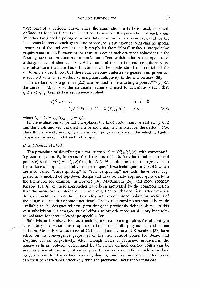
Fig. 1. Subdivision of cubic Bezier curve.
As examples for specific “halving” subdivision algorithms, we refer the reader to Figs. 1 and 2, which describe subdivision procedures for Bezier curves and for uniform 5-splines. The original cubic Bezier curve defined by P0P lP2P3 has been subdivided at the parameter value s = \ so that the same curve is now described as two articulated Bezier curves defined by PqPIPj P* and by P^P^P\P . At each level the Bezier subdivision algorithm consists of connecting midpoints of the previous polygon. The “halving” algorithm for uniform cubic 5-splines curves illustrated in Fig. 2 is performed similarly after the original polygon P0P iP1P7i is augmented with extra midpoint vertices P?, P^, P$.
Both of the above constructions generate a convergent, shape-preserving, sequence of piecewise linear approximations in which each new vertex is given recursively as a convex combination of two previous vertices. This leads to simple and fast algorithms for generating subdivisions. Since the convex hull property of 5-spline curves is not altered by subdivision, this characteristic of the 5-spline basis has been exploited to solve hierarchically for points of interaction between two 5-spline curves, or between two 5-spline surfaces, or between a curve and a surface. The general rule is simple: Recursively subdivide and test only when relevant convex hulls overlap. No intersection is possible if the convex hulls do not intersect. Since the parametric value of the curve is always known at the point of subdivision, the parametric value of an intersection found by subdivision can easily
Fig. 2. Subdivision of cubic 5-spline curve segment.
B-SPLINE SUBDIVISION 91
be known to within the tolerance of the testing criterion. That is, the interval containing the intersection is always known. A fuller discussion of these methods with more generality and rigor appears in [3, 19, 20, 21, 23].
The convergent properties of subdivision methods can be used as a method of curve generation itself, for the constructions lead to a close piecewise linear approximation to a smooth curve or surface, which is exactly what is necessary for driving a display or other numerical control machines. Several years ago Chaikin [7] proposed such a scheme, which he viewed as successively “cutting” off the corners of a polygon. Riesenfeld later proved that his “midpoint” construction actually yielded quadratic 5-splines with a certain intrinsic parametrization [35]. Recently Doo and Sabin [15] and Catmull and Clark [6] studied very intriguing local subdivision schemes for surfaces derived from meshes involving nonrectilin- ear topologies. All of the uses of subdivision for curve and surface generation substitute a recursively applied procedure for the more traditional use of a closed-form mathematical function.
3. DISCRETE B-SPLINES
In this section we extend and present the necessary theory of a discrete 5-splines so that it can be applied to the general area of subdivision in the remaining sections.
Discrete splines have been studied extensively. They were introduced by Mangasarian and Schumaker [28] as solutions to certain minimization problems involving differences instead of derivatives. They are connected to best summation formulas [29], and have been used by Malcolm [27] to compute nonlinear splines iteratively. Approximation properties of discrete splines have been studied by Lyche [24, 25], Discrete 5-splines on a uniform partition were introduced by Schumaker [37]. Discrete 5-splines on a nonuniform partition were defined by deBoor [13, p. 15].
Consider a piecewise polynomial written in terms of 5-splines Bik of order k:
n
f ( x ) = 2 P,Bik{x ) . (3.1)/= l
The knots r = { t , , . . . , rn+k} can be nonuniform and multiple. There are certain situations where it is useful to increase the degrees of freedom of / by adding additional knots r “ = {t,°, . . . , t " ) to the already existing ones. Suppose we let m = n + I and t = { ? , , . . . , tm+k} = r u t “ be the new knot sequence in nondecreasing order. With Njk the 5-splines on t, f can also be written as a linear combination of N1 Nm k with certain (unknown) coefficients dy.
m
f ( x ) = 2 djNjk(x ) . (3.2)j = i
We consider now the followingPr o b l e m . Given k, n, m, r , t, and { / >1, . . . , / >n} as above, compute d x, . . . , d m.
There are several ways to compute the dj's. For instance, we can choose m points
92 COHEN, LYCHE, AND RIESENFELD
p , , . . . , pm and solve the interpolation problem,
m2 djNj^Pi) = i — 1 ,2 ,.. . , m. (3.3)
7 = 1
If tj < pj < tJ + k, j = 1 , 2 t hen this set of linear equations has a unique solution The coefficient matrix is totally positive and banded, and it canbe inverted by Gaussian elimination without pivoting in Q(mk2) operations (see deBoor and Pinkus [12).
Alternatively one can use the quasi-interpolant of deBoor and Fix [11] to compute the d ? s. Thus if
A J = 7 r ^ 2 ( - l ) t " 1 )(« ; ) / (‘ - , - r)K ) , (3.4){K I). r = Q
where ay is any point in (tj9 tJ+k) and
k - 1
*j{y ) = n (y - tj+r), (3.5)r= 1
then
Xj N,k = 8,j = i= j>- 0, i =£j.
Therefore applying X; on both sides of (3.2) we have
dj = \jf, j = \ ,2,.. . ,m . (3.6)
This method of computing dj could be advantageous if / is given in its piecewise polynomial representation.
We will, not, however discuss these methods any further. Let us instead consider a third method. Here dj will be computed recursively. The method is similar to the subdivision scheme considered by Lane and Riesenfeld [23] for the special cases of Bezier curves (&-tuple knots) and for uniform knots. In fact, our method, which is valid for any knot configuration, reduces to theirs in these special situations. To start we note by linearity that
nd j = l l ocik(j )P i (3.7)
;=1
for some numbers aik(j).
To gain some insight we start by studying the cases k = 1 (step-functions) and k = 2 (piecewise linear functions).
Suppose first that k — 1. Then
nj{x) = 2 P,Bn(x),
i=i(3.8)

where
If
B-SPLINE SUBDIVISION
5 ,lO )= l , Ti < X < T i + ] ,
- 0 , otherwise.
where
then
f ( x ) = 2 djNjX(x ) ,7 = 1
Nj\(x) = 1 , tj < x < tj+ j ,
= 0, otherwise,
dj = p, , Ti < t j < T i/ + 1 *
Hence in (3.7) we have
= 1, T, ^ 0 < Ti+,’
— 0, otherwise.
We note that a n( j ) =Consider next the case k = 2. Then
where
Suppose
where
/(*) = 2 P t B , i ( x ) , 1= 1
5,.2(jc) = ( x - T , ) / (t, + 1 - T ,.), T, < X < ri + l ,
= U + 2 - * ) / ( t, + 2 - T ,+ 1) , T,.+ 1 < * < T,. + 2 ,
= 0, otherwise.
/“ i
t j < X < tJ + ,,W/20) = (* - / ;) / (?y+1 - /y),
= (f/ + 2 - * ) / (0 + 2 _ 0 + ') ’ 0+1 ^ < 0+2 >
= 0, otherwise.
(3.9)
(3.10)
(3.11)
(3.12)
(3.13)
(3.14)
(3.15)
(3.16)
(3.17)
93

94 COHEN, LYCHE, AND RIESENFELD
N ow if v and j are such that
then
Thus (3.7) is valid with
«,2(v) = (‘j+1 - T,) / (T/+i ~ T;)>
= (fi + 2 - tj+\)/ ( f i + 2 - T/+1),
= 0, otherwise.
We also note that «,-2( i ) = Ba ( tJ+ i)-We observe the interesting fact that the numbers a ik( j ) are related to the
5-spline 5 /(t for /c = 1,2. As we shall see the relation between a ik and Bik for k > 2
is not as simple as that for k = 1 and 2. In fact, a ik( j ) is a discrete 5-spline.The relation between 5-splines NJk on a partition {tj) and 5-splines Bik on a
(coarser) subpartition ( t J is given in the following theorem.
T h e o r e m 1. For all x we have
Uj can be chosen anywhere in \tj, tJ+k), and, Ti+k\<i>jk denotes a divided difference.
Remarks.
1. a ik( j ) is called a discrete 5-spline.
2. The number a ik( j ) in (3.7) are the discrete 5-splines given by (3.21).
Proof. From (3.1) and (3.20) we have
where a ik( j ) is given by (3.21). Comparing this with (3.7) the statement follows.
mBik(x ) = 2 otik(j)N Jk{x ) , i = l , 2 , . . . , m . (3.20)
where
a , j ( j ) = ( W ~ Ti)[Tn---,Ti + k]$Jk ,
<t>jk(.y) = (y - ajf+ %k(y)>
(3.23)
(3.22a)
and where %k(y ) is given by (3.5). Here
(y ~ a j f+ = 1, y > a p= 0, otherwise,
n n m/ ( * ) = 2 P,B,k{x ) = 2 2 P ^ kU )N Jk(x )
m n
j ~i L / = i J
B-SPLINE SUBDIVISION 95
3. For k = 1 we have from (3 .2 1)
«/iU ) = (Tj+ i ~ <J;)° - (t, - a,.)° , (3.22b)
which agrees with a n ( j ) given by (3.13) for any a } G [tj, tJ + l ). Similarly for k — 2 we find
« / 2 0 ) = [ T i + 1 , r l + 2 ]<l>J2
with
^ 2( 7 ) = ( .v - « / ) + - tJ + , ) .
This can be seen to agree with a i2( j ) given by (3.19) for any a,- £ [/., / , +2).
4. Identity (3.20) can also be found in deBoor [13, p. 15]. However, deBoorused
k- 1<t>jk(y) = I I ( ^ - 0 + r ) +
r = 1
to define a lk( j ) in (3.21). With this <j>Jk it was not clear to us how to interpret (3.21) for multiple t ’s.
To prove Theorem 1 we need two lemmas. The first lemma is due to Marsden [30].
L e m m a 1. F o r a n y y £ IR a n d a n y x G [/fc, tm + l ) w e h a v e
m
( y - * ) * ' ' = 2 * jk { y ) N Jk{ x ) , (3.23)
where % k( y ) is given by (3.5).P r o o f (deBoor [14]). For k — 1, (3.23) takes the form 1 = S J = iA^,(x), which
follows from (3.11). For k > 2 we use the recurrence relation (deBoor [14], Cox [9])
Njk(x ) = ( * ~ t j)Q j,k - i ( * ) + ({j+k - x)Q J+uk. l(x ) , (3.24)
where
Q j k ( x ) = N j k ( x ) / { { j + k - t j ) , tJ + k > tj,
= 0, otherwise. (3.25)
Denoting the right-hand side of (3.23) by £k we find
m
$k = 2 ^ / f c 0 0 [ ( * ~ t j)Q j.k -i(x ) + (*j+k ~ * ) G / + i , * - i ( * ) ] -7 = 1
Since x e [tk , tm + l ) we have ~ Q m + \ .k ~ \(x ) = 0- Hence rearranging the
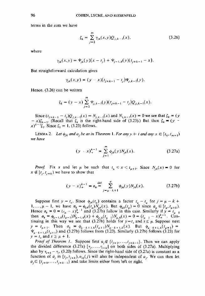
96 COHEN, LYCHE, AND RIESENFELD
m
$k = 2 yjk(x’y)Qj,k-i(x)’ (3-26)7 = 2
where
Y/*(*>->') = % k(y )(X - 0 ) + * 7 - l .* ( j ' ) ( /7 + * - l _ *)•
But straightforward calculation gives
Yjk(x >y) = (y - x )(tj+k- i -
Hence, (3.26) can be written
m
h = (y ~ x ) 2 ^/,*-i(j')(o+*-i _ 0)^7 ,*- i(x )-7 = 2
Since (tJ+k_ l - /,•)£?,-*_ , ( * ) = A ^ . ^ x ) and TV, . * _ , ( * ) = Owe see that £k = (.y— x)£k_ v (Recall that is the right-hand side of (3.23).) But then £k = (y — x ) * _1f,. Since f, = 1, (3.23) follows.
Lemma 2. Let <j>Jk andaj be as in Theorem 1. For anyy E t and any x G \tk,tm+]) we have
m
(y - x ) k~' = 2 <t>jk(y)Njk (x )- (3.27a)7 = 1
Proof. Fix x and let p. be such that < x < Since NJk(x ) = 0 for x & [tj,tj+ k) we have to show that
def ^(y - x ) k+ 1 = °k = 2 fyk(y )Njk (x )- (3.27b)
j = y.-k+\
Suppose first y = Since <t>jk(tIL) contains a factor t — t for j = p. — k + l , . . . ,ju. - 1, we have ak = ^ ( t ^ N ^ x ) . But ^ ( ^ ) = 0 since aM G > tp + k)-
Hence a* = 0 = (iM — x )k+~' and (3.27b) follow in this case. Similarly if y = t x then ak = , * ( ^ _ , ) ^ _ 1>( x ) + <Jv,*(^_ ^ ^ ( x ) = 0 = ( ^ _ , - x ) * - 1 . Continuing in this way we see that (3.27b) holds for y = ts and s< p.. Suppose next
y = ^+i- Then ° k = ^-*+i,*(^+i)^-*+i,*(^)- But <#>„-*+i,*(^+i) =¥,,_*+1 ,*;(^+1) and (3.27b) follows from (3.23). Similarly (3.27b) follows (3.23) for y = ts and s > p + 1.
Proof o f Theorem 1. Suppose first a , £ {^+ i»• • •»tj+k~\}- Then we can apply the divided difference (3.27a) [t,-, . . . , Ti+k] on both sides of (3.27a). Multiplying also by ri+k — r„ (3.20) follows. Since the right-hand side of (3.27a) is constant as a function of a, in [tj,tj+ k) ,a ik( j ) will also be independent of a.. We can then let Oj El ( tJ + tJ + k [} and take limits either from left or right.
terms in the sum we have

B-SPLINE SUBDIVISION 97
We next prove a recurrence relation for the <xik( j ) . A similar recurrence relation for uniform t's has been given by Schumaker [37] and Lyche [24].
Theorem 2. Suppose rj+k> and that a ik( j ) is given by (3.21). Then
a i \ (J ) ~ I - t , < t j < Ti + j ,
= 0, otherwise. (3.28)
Moreover for k > 2 and all i,j,
a ik (J ) = ( !j + k - 1 ~ + ( Ti+k ~~ t j+ k - l)P i+ l,k - l( j) ’ (3.29)
where
P ikiJ) = a ik ( J ) / ( T, + k ~ T/)> Ti + k > Ti’= 0, otherwise. (3.30)
Proof. Equation (3.28) follows from (3.22b). To prove (3.2.9) we proceed as in [14], applying the L eib n iz’ rule to the product <Pj/c( y ) — (y —
def
tj+ k-O fy .k-iiy ) = g (y )'K y )- Then
i-¥k
r = i
Since [r,]g - g(t,) = (r, - ?;+*_, ) , [T ( , r i + 1 ] g = 1 and [ t r , ] g = 0 for r > ; +1, we obtain
[ T,, . . . , t ,+1 ^ = g ( T,.) [ T i , . . . , r i + k ] h + [ T, + J , . . . , r ,+* ] h .
By the definition of divided differences
( T/+* - Ti ) [ Ti ’ - - - > Ti + k ] h = [ T;+i>--->T/+*]/l ~ [ Ti r i + k - i ] h -
Hence
a i k ( J ) = ( T/+* “
- 0,. - tj+ k _ i ) ( [ r i + l , . . . , r i +k ] h - [ r n . . . ,Tl +k _ { ] h )
+ (t/+* ~ Ti) [ r/+ T,.+fc] A
= (T ,.+/t_ , - t i) [ T i , . . . , T i + k .- i ] h + ( r i+ k - t ( ) [ t , + 1, . . . , t i+k\h.
But this is precisely identity (3.29). Note the similarity between (3.29) and the recurrence relation for Bik,
Blk(x ) = (x - Ti)Cj k_ i(x ) + (rl+k - x)Ci+uk_ i(x ) , (3.31)

98 COHEN, LYCHE, AND RIESENFELD
Qt(*) = B i k ( x ) / ( r i +k - rf), r i+ k > Ti ,
= 0, otherwise. (3.32)
Thus the discrete splines a ik( j ) have properties very similar to those for Bik. We collect some properties of a ik( j ) in a corollary to Theorem 2.
C o r o l l a r y . Let otik( j ) be as in Theorem 2. Then
(A) For 1 < j < m let /jl be such that < ty < tm+1. Then a ik( j ) = 0 i & {jn — k + 1 , . . . , jli};
(B) a ik{ j ) > 0, all i ,j;
(C) '2ni=\a ikU) = W < tj < t„+v
Part (A) says that for each j there are at most k discrete B-splines a k+l<k( j ) , , a^ k{ j ) with a ( possible) nonzero value.
Proof. By (3.28), (A) follows immediately for k = 1. Suppose (A) is true for A: — 1; i.e., only a ll_k + 2 k_ ]( j ) , . . . , a flk_ l( j ) can be nonzero. By the recurrence relation (3.29) it is clear that only oc)X_k+lj c{ j ) , . . . , ct^kU ) can be nonzero. Hence (A) follows by induction.
To prove (B) we need a slightly stronger version of (A).
(A'). If tj < Tt or tj+ k_ l > Ti+k then a lk( j ) = 0. The fact that a lk( j ) = 0 for tj < 7} is clear from (A). Suppose tj+k _, > Tj+k. If k = 1 then a n( j ) = 0. We proceed by induction. Since tj+k_ x > ri+k we have tj+ k_2 > Ti+k_ v Hence A .* -iO ') = 0. Also, if tj+ k_ ] > Ti+k then tJ+k_2 > Ti+k and f t +li* _ , 0 ' ) = 0. Hence by (3.29) we have a ik( j ) = 0 for tj+ k_ ] > Ti+k. This completes the proof of (A'). To prove (B) we note that by (A'), we only have to prove that a ik( j ) > 0 for / . > t, and tJ+k_ i < Ti+k. But then all factors in (3.29) are nonnegative.
Finally, to prove (C) we note that
n m1 = 2 Bik(x ) = 2 NJk(x ).
i -l j ~l
Thus by taking dj and all Pt's equal to 1 in (3.7), (C) follows.
We return now to the problem of computing dj in (3.7) once the Pt's are known. Writing (3.7) in the form
n
d ( j ) = 2 P i*ik(j) i = 1
we see that d ( j ) is a discrete spline, i.e., a linear combination of discrete B-splines. The fact that discrete splines have local support is proved in Corollary A and used in Algorithms 1 and 2. The similarity between the recurrence relations (3.29) for a ik{ j ) and (3.31) for Bik therefore makes the computation of d ( j ) very similar to
where

B-SPLINE SUBDIVISION 99
the computation of f ( x ) for some x wheren
f ( x ) = 2 PiBik(x ) . i= 1
This leads to the following algorithms:A l g o r i t h m 1. F o r integers k > 2 a n d j , ji let Tfl+2_ k , . . . , T/1 + k _ i a n d
tj + l , . . . , t J+k_j b e g iv e n s u c h that
V 2_k < • • • < T(1< tm+1< • • • < (3.33)
(3-34)
This algorithm computes o,r = a ,r( j ) given by (3.21) or (3.29) r = 1 , . . . , k ; i = n +1 These are all the discrete 5-splines of order < k that can be nonzerofor the given j .
(1) a(ju, 1) = 1, ju2 = jn
(2) For r = 1 , 2 , . . . , k — 1
(i) beta_ 1 = 0, tj = t( j + r )
(ii) For i = ^2 , ^2 + I , . . . , ft(a) d\ = tj - r (/'), d 2 = r ( i + r ) - tj
(b) beta = a ( i , r ) / ( d 1 + d l )
(c) a ( i — 1 , r + 1) = «/2*beta + beta_l
(d) beta_l = ^l*beta
(iii) a(fi, r + 1) = beta_ 1
(iv)ju2 = ju.2 — 1.
Algorithm 1 can be used to computen
d ( j ) = 2 « i k ( J ) P i ’
i= 1for if tm < tj < tm+1
d { j ) = 2 «ik( j)P , (3-35)i = / i — k + 1
and the values a ik( j ) are available from Algorithm 1.There is an alternative way to compute d ( j ) given by (3.35) which parallels
Algorithm 1 in [23]. To derive it we have by (3.29)
d ( j ) = 2 p ia i k U ) = 2 P { ( t J + k _ , - T , . ) / ? , )i = (X — k+ 1 i = fi — k + \
+ (Ti + A: _ fz+fc-OA'+l.t-lCv')]'
Since /?„_*+! , *- , ( . / ) = h + i ,k - iU ) = 0 by (A) in the corollary, we have
d ( j ) = 2i=H-k+2
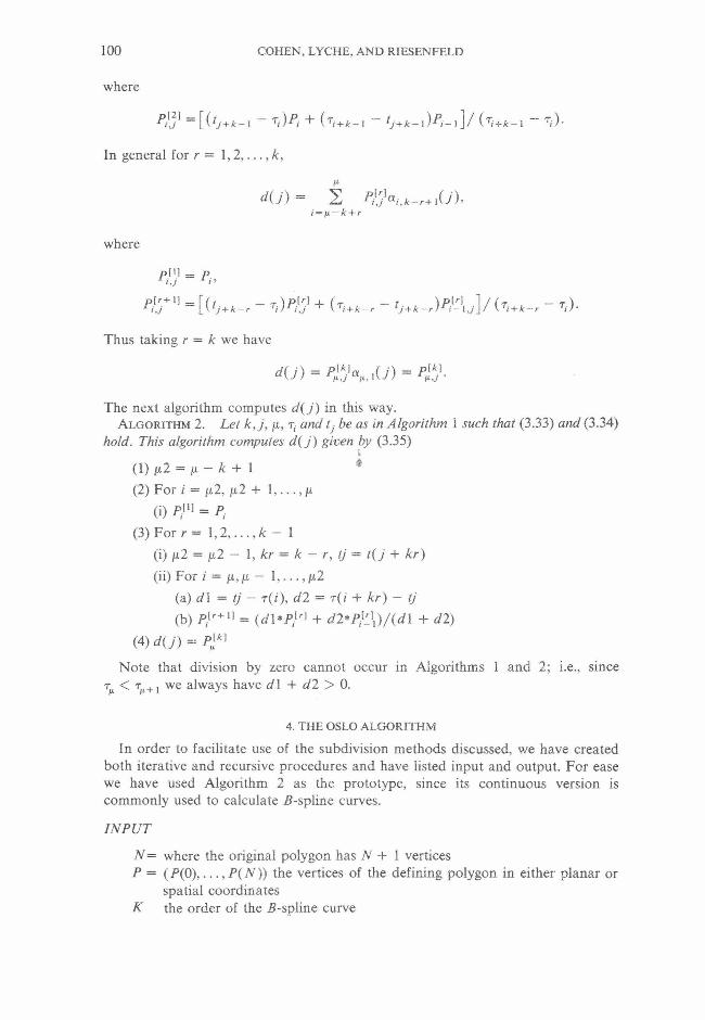
100 COHEN, LYCHE, AND RIESENFELD
where
i + k — 1
In general for r = 1 , 2 , . . . , k,
i,k — r+ 1(j)>i = jx — k + r
where
Thus taking r = k we have
The next algorithm computes d ( j ) in this way.A l g o r i t h m 2. Let k , j , p, rt and tj be as in Algorithm 1 such that (3.33) and (3.34)
hold. This algorithm computes d ( j ) given by (3.35)
(1) \>.2 = n — k + 1 *
(2) For i = /i2, jx2 + 1 , . . . , jix
(i) P/'l = P,(3) For r = 1 , 2 , . . . , k - 1
(i) jj,2 = fi2 — 1, kr = k — r, tj = /( / + A.r)
(ii) For i = ft, fi — 1 ,..., /x2
(a) i/I = tj — r ( / ) , d2 — t(i + A:r) — tj
(b) = ( J } * p . l r) + </2*7»yj)/(rfl + rf2)
(4) J(v) -
Note that division by zero cannot occur in Algorithms 1 and 2; i.e., since Tn < Tn+i we always have d 1 + d2 > 0.
In order to facilitate use of the subdivision methods discussed, we have created both iterative and recursive procedures and have listed input and output. For ease we have used Algorithm 2 as the prototype, since its continuous version is commonly used to calculate B-spline curves.
N = where the original polygon has N + 1 verticesP = (P(0 ) , . . . , P(N )) the vertices of the defining polygon in either planar or
spatial coordinates K the order of the B-spline curve
4. T H E O SL O A L G O R IT H M
INPUT
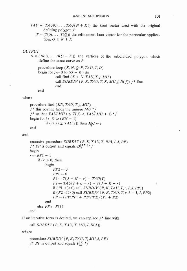
B-SPLINE SUBDIVISION 301
TAU = (T A U ( 0 ) ,T A U ( N + K )) the knot vector used with the original defining polygon P
T = (T(0 ) , . . . , T(Q)) the refinement knot vector for the particular application, Q > N + K
OUTPUTD —■ (D (0),. . . , D(Q — K )) the vertices of the subdivided polygon which
define the same curve as P.
procedure loop (K , N, Q, P, TA U ,T,D ) begin for j <- 0 to (Q - K ) do
call find (K + N, TA U, T ,j, MU)call SUBDIV ( P , K, TA U, T, K, MU,j, D (j)) / * lineend
end
where
procedure find ( KN, TA U, T,j, MU)/ * this routine finds the unique MU * // * so that TAU(MU) < T ( j) < TAU(MU + 1) * / begin for i <— 0 to (KN — 1)
if (T O ) > TAU(i)) then M U /end
and
recursive procedure SUBDIV ( P, K, TA U, T, RPl, J, J , PP)/ * PP is output and equals D }*pl] * / beginr RPl - 1
if ( r > 0) then begin
PP2 <- 0 PP l <- 0PI T (J + K - r ) - TA U (I)P2 <- TA U(I + k - r ) - T (J + K - r ) \
if (P I < > 0 ) call SUBDIV (P, K, TAU, T ,r ,I,J,P P \ ) if (P 2 < > 0) call SUBDIV (P, K, TA U, T, r, 7 - 1 , 7 , P P l) PP^(P\*PP\ + P2*PP2)/(P\ + P2)
endelse PP<r-P(I)
end
If an iterative form is desired, we can replace / * line with
call SUBDIV ( P, K. TA U, T, MU, J , D (J ))
where
procedure SUBDIV (P, K, TA U. T, MU, J , PP)/ * PP is output and equals P f f * /

102 COHEN, LYCHE, AND RIESENFELD
beginfor I ^ ( M U - K + 1) to MU T E M P (l,I) * - P (I);
for r <— 1 to K — 1 do begin
for i <— (MU — k + 1 + r) to MU begin
T l <- T (J + K - r) - TA U(i)T2 <— TAU(i + K — r) — T (J + K - r )TEMP(r + l ,i)< -(T l*T E M P (r ,i) + T2*TEM P(r,i - 1) / ( T l + T2)
endend
/*/*<— TEMP(K, MU) end
5. APPLICATIONS OF THE OSLO SUBDIVISION ALGORITHM
The Oslo algorithm described in the previous section has many applications in CAGD, computer graphics, and numerical analysis. In this section we will give some sample extensions and generalizations that are made possible by the power to perform subdivision on arbitrary refinements. It is evident to the authors that the optimal choice of the refinement vector I in many applications is a freedom that can be exploited considerably beyond what is proposed here. The refinement choice may also be optimized for a particular application in which additional a priori knowledge is available. So the following algorithms might be viewed as starting points for the construction of more specialized or sophisticated (intelligent) algorithms based on the same theory. This section is meant to suggest a collection of algorithms whose optimal forms cannot be adequately developed within the scope of this paper.
A p p l ic a t io n 1. Add a new (pseudo)knot at a prescribed point and calculate the new control polygon.
This application is an essential step in Knapp’s approach to designing curves and surfaces by introducing more flexibility, i.e., control points, in regions where finer specification is required [17]. The calculations for the new vertices in (a) are carried out in detail for this application, so that it can serve as an example in computing with the Oslo algorithm.
(a) The original curve is an open cubic B-spline curve with r = (0 ,0 ,0 , 0, 1, 2, 3, 3, 3, 3). A pseu dokn ot is added at 1.3, so t = (0, 0, 0, 0 , 1 , 1 . 3 , 2 , 3 , 3 , 3 , 3 ) .
Solution. Since it is cubic K = 4.
r = ( 0 , 0 , 0 , 0 , 1 , 2 , 3 , 3 , 3 , 3 ) .
N + K = 9, so N = 5 and the original polygon is P = (P0, P^,. . . , P5). Also, t = ( 0 , 0 , 0 , 0 , 1 , 1 . 3 , 2 , 3 , 3 , 3 , 3 ) so Q = 10 and D = (D0, . . . , D6).

t3 = 0 < tj < t4 = 1,
so Dj = P \ y,j = 0 , 1 ,2 , 3 .
Now let j = 0.
^ 3 ,o '= [(^1 — t 3 )^ >3,30 ( T3 + l ~ h ) P $ ] / ( T4 ~ t 3 )
= [(0 - 0 )4 30! + (1 - 0 )/foy i
= t( 2 - t2)P% + (U - w ' o 1] / ^ - r2)
= [(0 - 0)P™ + (1 - 0 ) P $ ] / 1
~ Pl20 = [(^3 ~ T j r U + (^4 — ^3)^0,o]/(t4 — Tl)
= [(0 - 0)P\'l + (1 - 0 ) P $ ] / 1
B-SPLINE SUBDIVISION 103
Now in procedure loop, \x = 3 fory = 0,1,2,3 since
Therefore D0 = P0.
Let j = 1.
P \ y = [(^2 — t 3 )^ 3 ,3/ ■*" ( t 4 ~ ^2)^ >2,3 ] / ( t 4 ~ T3 )
= [(0 - o)pw + (1 - 0)/>2'3,)]/i
= ^ 2 ,V = [(^3 — r2 ) P x \ + ( T4 _ h ) P \ 2\ } / ( r4 ~ t 2 )
= [ (0 ,0 )P '2l + (1 - 0)/>|2’] / l
= P ] 2] = [(?4 Tl)^>l,1] "*■ ( t4 — 4 )^0,'l ] / (T4 ~ Tl)
= [(1 - 0)Pfl + (1 - l jp ^ i/ d - 0)
= = Pi-
Therefore Z), = Px.Let j = 2.
P % 2 ~ [(^ 2 + 1 ~ J3 ) P x 2 ( t 4 — ^3)P\^2 ] / ^T4 — t 3 )
= [(0 - 0 )P {321 + (1 - 0)P™]/\
= * $ = [( 4 - t2)P $ + (t4 - *4)P $ ] /(t . - t2)
= [(1 - 0)P $ + (1 - 1 )P{22']/1
= P \ 22 = t ( ?5 ~ T2 )^ 2 ,2 + ( t 5 ~ ti ) P \ ]\ / (T5 — T2 )
= [1.3 P\}\ + 0.7P[|l] /2 .
Therefore D2 = 0.65P2 + 0.35 P{.
Let y = 3.
P ^ = [(<4 - ^ ) ^ 3 |33l + (T 4 - U ) P ^ ] / ( U ~ T3 )
= [(1 - 0 ) />3[33l + (1 - l)/>j3' / l
= ^3,33 = I ( * 5 ~ t3 )^ >3,23 + ( t 5 — 5 ) -^2 ] / ( T5 ~ T3 )
= [(1.3 - 0)/>3[23] + (2 - l.3)P{\']/2
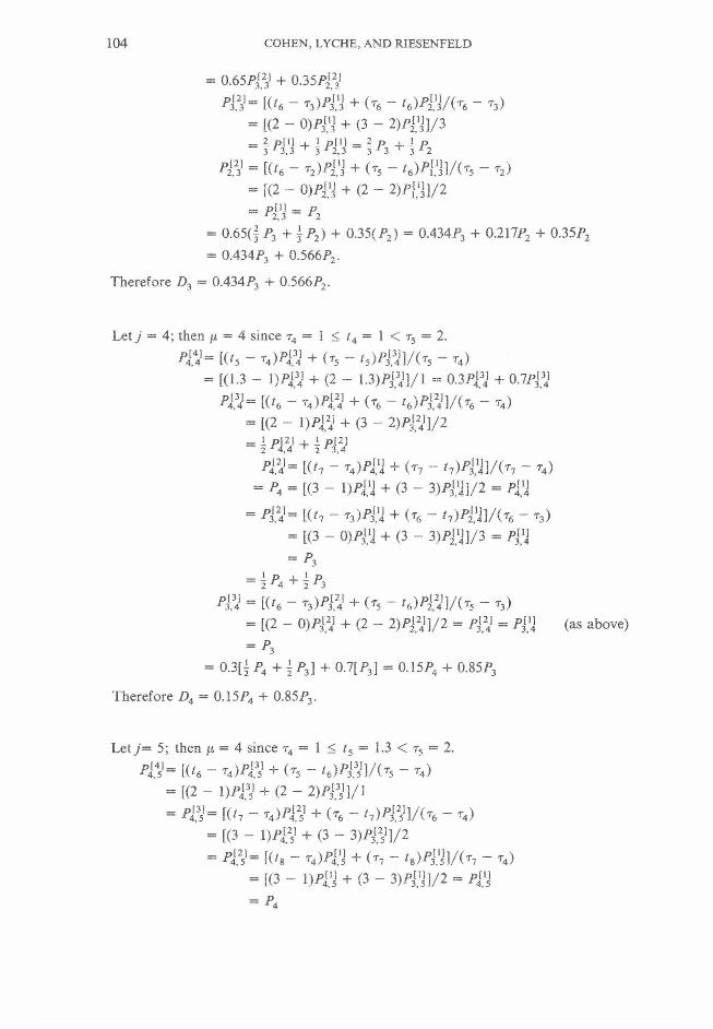
104 COHEN, LYCHE, AND RIESENFELD
= 0.65 Pj2 + 0.35 P2[23]
3,23 ~ t(?6 — r3)^3,3 (t6 ~ (T6 ~ T3)
= [(2 - 0)4'1 + (3 - 2)P2l']]/3
= I P[l] + A p[l] = 1 P + i P3 3,3 3 2,3 3 3 3 2
= t(^6 — T2 )^ 2 ,3 + ( T5 ~ ] / ( T5 _ T2 )
= [(2 - 0)4 'J + (2 - 2)pf']]/2
= = ^2
= 0.65(f P3 + ~ P 2) + 0.35(P 2) = 0.434P, + Q.217P2 + 0.35P2
= 0.434P3 + 0 .566P2.
Therefore Z)3 = 0.434P3 + 0.566P2.
Let j ~ 4 ; then ju = 4 since r4 = 1 < /4 = 3 < x5 = 2.
^4,44 ~ [(^5 — T4 )^ 4 ,34 + ( T5 — s )^ >3,3J ] / ( T5 — T4 )
= [(1.3 - l )P j34! + (2 - 1 . 3 ) F $ ] / 1 - 0.3P4[3J + 0 .7 P $
4 4 = K '« - ^ ) A ‘ 24I + (T 6 - /6 ) ^ ] / ( T 6 - T4 )
= [(2 - l )P j24i + (3 - 2 )P '24l ] /2
^ = I(<7 - ^ J . ' J + (t7 - h )P \ ]j]/(T7 - T4)
= P4 = [(3 - 1)P4! 'J + (3 - 3 )P j‘] ] / 2 = P],1]
= 3,41== [( 7 — T3)^3,4 + (t6 — ,7)^>2,4l/(T6 ~ T3)
= [(3 - 0)P3"j + (3 - 3 )P j‘J j /3 = Pj.'j
= ^3
= 2 P4 + j P3
= [(^6 ~ T3 )^ 3 ,4 + ( T5 ~ f 6 )^ 2 ,24 ] / ( t 5 — T j)
= [(2 - 0 )P j24i + (2 - 2)P2l241] /2 = P j2’ = P j’J (as above)
= ^3
= 0 .3 [i P4 + | P3] + 0.7[P3] = 0.15P4 + 0.85P3
Therefore D4 = 0.15P4 + 0.85P3.
Let j — 5; then ju = 4 since r4 = 1 < t5 = 1.3 < r5 = 2.
P J ."V = f(^6 ~~ T4 )^ 4 ,35 ■*" ( t5 ~ 3 / ( T5 — T4 )
= [(2 - 1)P4|35' + (2 - 2 )P j35! ] / l
= p jy = [(/7 — T4)P42* + ( t6 — / 7)P325 ] / ( t6 — t4)
= [(3 - l )P j25' + (3 - 3 )P j25i] /2
= A [,V= f( 8 — T4)^4,l5 (T~ ~ t$)P\ \\/(t7 - r4)
= [(3 - 1 )P' ‘‘ + (3 - 3)Pj,1l ] /2 = P l ‘1
= P4
B-SPLINE SUBDIVISION 105
Let j = 6; then n = 5 since r5 = 2 < t6 = 2 < t6 = 3.
^5*6 = [( * 7 — t 5 )^ 5 ,36 + ( T6 — ( T6 ~ T5 )
= [(3 - 2)/>5>36l + (3 - 3)P j36' ] / l
= ^5,6I = t ( ?8 — T5 )^ 5 , ft' + ( t 7 — ^8>/>I.6 1] / ( T7 ~ T5 )
= [(3 - 2 )P $ + (3 _ 3 ) P # ] / 1
= A [6= [(#9 - ^ ) 4 ,6) + K - f9) ^ ] / ( T 8 - Tj)
= [(3 - 2 ) Jp f |l + (3 - 3 ) ^ ] / l =
= ^5
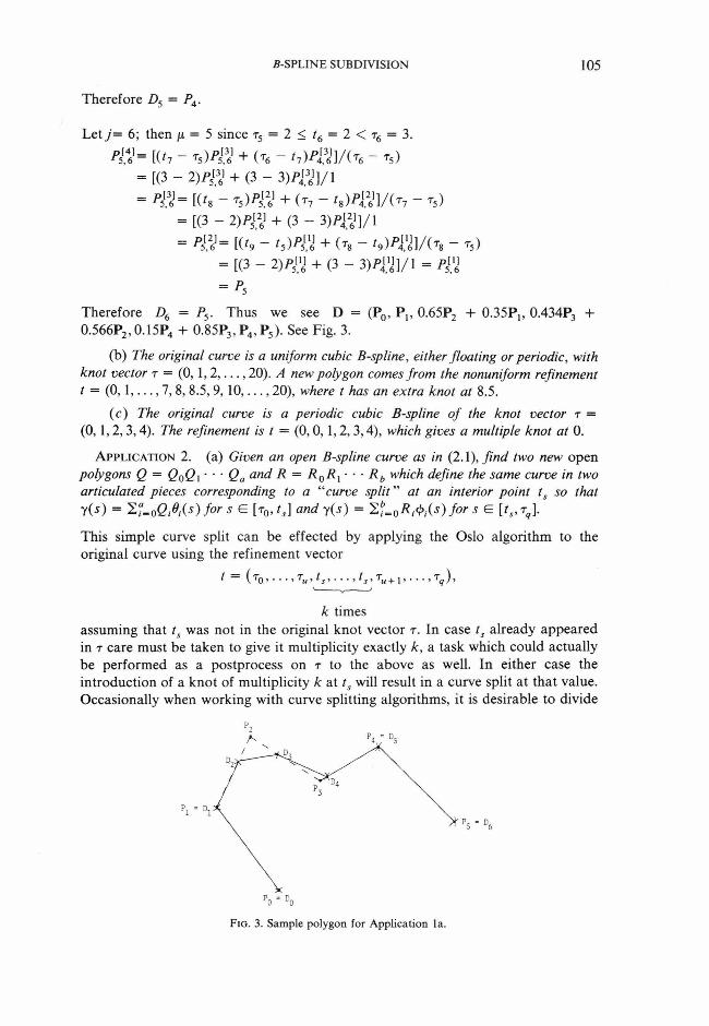
Therefore Z>6 = P5. Thus we see D = (P0, P ,, 0.65P2 + 0.35P, , 0.434P3 + 0.566P2, 0.15P4 + 0.85P3, P4, P5). See Fig. 3.
(b) The original curve is a uniform cubic B-spline, either floating or periodic, with knot vector r = (0, 1 , 2 , . . . , 20). A new polygon comes from the nonuniform refinement t = ( 0 , 1 , . . . , 7, 8, 8.5, 9, 1 0 , . . . , 20), where t has an extra knot at 8.5.
(c ) The original curve is a periodic cubic B-spline o f the knot vector t = (0, 1 ,2 ,3,4) . The refinement is t = (0,0, 1,2, 3,4), which gives a multiple knot at 0.
A p p l i c a t i o n 2 . ( a ) Given an open B-spline curve as in (2A), find two new o p e n
polygons Q — QoQ\ - • ' Qa and R — R 0R { • • • R h which define the same curve in two articulated pieces corresponding to a “curve split” at an interior point ts so that y(s) = 2f_0Q ,0 ,(s)fors G [iq,*,] and y(s) = 2?=0R ^ ( s ) fo r s G [ts, tJ.
This simple curve split can be effected by applying the Oslo algorithm to the original curve using the refinement vector
* (*7*0 ’ * * * ’ s ’ * ' * ’ s ’ + 1 ’ * * * ’ ’
k timesassuming that ts was not in the original knot vector t . In case ts already appeared in t care must be taken to give it multiplicity exactly k, a task which could actually be performed as a postprocess on t to the above as well. In either case the introduction of a knot of multiplicity k at ts will result in a curve split at that value. Occasionally when working with curve splitting algorithms, it is desirable to divide
Therefore D5 — P4.
F ig . 3. Sam ple polygon for A pplication la .

106 COHEN, LYCHE, AND RIESENFELD
the original curve y (s ) into separate curves which are represented in a similar form. This can be achieved by dividing the refined knot vector t into two subpieces
h ( To > • ■ • ’ * ■ • • > ts) and t r ( ts, ts, . . . , ts, tu+ j , . . . , )
k times k timesfor the left and right subpieces, respectively. Furthermore, since the relative spacing of the knots only is of importance in determining the shape of the 5-splines, it is straightforward to normalize the pieces so that the new knot, vectors both begin at a parameter value of 0. Division by the largest knot is also possible to normalize the parameter range, but this is usually not done in practice, since the benefits of doing so are not very important.
(b) Given a closed B-spline curve as in (2.1), split the curve into open B-spline curve points at ts.
This problem is very similar to Part 2a above, and can be treated in an analogous manner by introducing a new knot of multiplicity k at the parameter value ts in the refinement vector t. This procedure is sufficient to specify an open polygon, if the knot vector is treated in a modulo fashion. Otherwise, it is simply a matter of rearrangement to string out the knots to form an ascending knot vector with appropriate multiplicities at the beginning and end knots.
(c) Divide a closed B-spline into two open B-spline curves.
This problem can be viewed as a combination of the process described in Application 2b followed by 2a.
Application 3. Determine the parametric values o f the points o f intersection o f two B-spline curves y ^ s) and y2(t) o f orders k x and k 2 defined over knot vectors r, and t2, respectively.
This algorithm, in its most basic form, is a straightforward generalization of Algorithm V for Curve Intersections in Lane and Riesenfeld [23], Using the Oslo algorithm, it is possible to split y^ s) and y2( 0 at their parametric midpoints by adding new knots of multiplicities M, and M2 at the parametric midpoints, in the case that the convex hulls for y ^ s) and y2(r) overlap. If the convex hulls do not overlap, no curve intersection is possible. This basic procedure involving the above curve-splitting technique can now be applied recursively, adopting all of the refinements including tests for linearity of the subpieces described in [23] until all intersections are found to within a prespecified tolerance. Strategies for splitting at points other than midpoints are intriguing, but the pitfalls of such bolder strategies are many. A more complete analysis of these advantages and disadvantages is a topic for another paper. Here we shall only point out that the structure, but not the performance, of such variants is basically the same.
Application 4. Extend the Lane-Riesenfeld algorithms for rendering B-spline surfaces.
The power to split nonuniform 5-spline curves leads very directly to the power to split tensor product 5-spline surfaces in a manner completely analogous to the approach taken by Lane and Riesenfeld in [23]. Essentially they recursively
B-SPLINE SUBDIVISION 107
subdivide, say into four subpieces, until matters of intersections and visibility are reduced to unambiguous, piecewise linear cases. A simple frame buffer algorithm for generating a picture of a 5-spline scene then consists of sending a parametric line through the eye and a pixel into the 5-spline scene. Subdivision can be used to compute the nearest and subsequent intersections of the parametric line with the scene. Alternatively, one can invoke subdivision until the surface is determined to be sufficiently locally flat, and then resort to any standard polygon-rendering algorithm to compute the corresponding image for display. This, too, is a frame buffer algorithm, as the order of image generation is not generally in scan line order. All of the improvements that apply to the Lane-Riesenfeld algorithm can also be applied in this more general setting. The Oslo algorithm for subdividing arbitrary 5-splines serves to extend the class of 5-splines to which the L an e- Riesenfeld algorithms can be applied. The structure of the algorithms remains identical.
Application 5. Extend the Lane-Carpenter algorithm.
The Lane-Carpenter algorithm looks at all surfaces that intersect the “current scan line,” and then progressively subdivides all of those “active surfaces” until they become either “nonactive” or sufficiently close to planar that they can be treated as polygons in a Watkins-like manner. Inasmuch as the Oslo algorithm allows for the splitting of nonuniform 5-spline surfaces, it is clear that this can be used to extend the Lane-Carpenter algorithm to this wider class of surfaces. The Oslo algorithm can be used to split the active surfaces into four subsurfaces by splitting at the parametric midpoints along each parameter domain. The remaining portions of the Lane-Carpenter algorithm can be applied without alteration.
Application 6. Generate curves and extend the deBoor-Cox algorithm.
In [20] it is shown that the polygon associated with each refinement converges to the 5-spline curve as long as the mesh size of the refined knot vector goes to zero. Thus one can reasonably use a closely refined knot vector to generate a polygon which is useful as a representation of the curve on a graphics display, since a piecewise linear approximation is usually used for display purposes anyway. It was observed by Lane [18] that the Oslo Algorithm actually specializes to the deB oor- Cox algorithm when the refinement consists of adding a new knot of multiplicity k (the order). This observation further shows that the d eB oor-C ox algorithm, in its intermediate recursive calculations, generates vertices corresponding to a split of the 5-spline curve at the point of evaluation for the deB oor-C ox algorithm. These properties follow directly from observing when the two formulas become identical. One could consider this application as an extension to Chaikin’s algorithm as well, since Chaikin’s algorithm was shown to produce quadratic 5-spline curves [35].
Application 7. Convert from B-spline to piecevnse Bezier form and generalize constructions o f Bohm and o f Sablonniere.
As the Bezier curve form is purely polynomial and simpler to understand and use, it is occasionally desirable to convert to it from the 5-spline representation. This problem has been studied for specialized cases and algorithms for these have been developed by Bohm [4] and by Sablonniere [36]. The Oslo algorithm is useful for providing the general construction for converting nonuniform 5-splines to an

108 COHEN, LYCHE, AND RIESENFELD
equivalent piecewise Bezier representation for any order k. This application of the Oslo algorithm follows immediately from the fact that the Bezier representation is actually a special case of the B-spline form in which there are knots of multiplicity k at each end of the curve and no interior knots. This necessary condition can be met for any B-spline curve simply by refining the knot vector so that each knot appears with multiplicity k.
A p p l ic a t io n 8. Produce a contouring algorithm for B-splines.
In many applications in engineering and other areas, it is required that a series of contour plots for a B-spline surface be made. These contours may represent fuel levels in an airplane wing, station curves of a ship’s hull, or water lines on a cargo ship. In any case, contours can be computed as the intersection of two B-spline surfaces, one being the model for which the contours are desired and the other being a parametric plane. Stating it in this way, we have reduced the problem of producing contours to the problem of intersecting two B-spline surfaces, a problem to which the Oslo algorithm has already been successfully applied.
A p pl ic a t io n 9. Generate refraction and shadow algorithms for B-spline surfaces.
In order to produce very realistic pictures of B-spline surfaces representing transparent objects, it is helpful to include refraction calculations to simulate the proper distortion which would be present in a corresponding photograph. This calculation is an easy one involving only the normal to the surface at each pixel and a table of the indices of refraction for the surfaces in the scene being rendered. Certainly such information can be included in a rendering algorithm based on the Oslo algorithm, for the normal vector is easily calculated for a planar polygon produced by the Oslo algorithm. Similarly shadow algorithms require knowledge about the visibility of surfaces from the vantage point of the light source rather than the viewer. Anything that is not visible from the light source is shadowed. Seen in this way, a shadow algorithm is just an invocation of a hidden surface algorithm, an application which has already been discussed in Applications 4 and 5.
A p p l ic a t io n 10. Find the zeros and extrema o f a polynomial spline function.
Normally the problem of finding these critical points of a spline are treated by viewing a spline function as piecewise polynomial and solving the problem for each polynomial span. Clearly subdivision techniques like those employed by Lane and Riesenfeld can be extended to finding the answer globally for the whole spline without decomposing it into constituent polynomial pieces. The formulation and analysis of this approach are a subject of further research by the authors.
A p p l ic a t io n 11. Generate nontensor product surfaces.
Recently some intriguing procedures for generating an approximating surface to a topologically nonrectangular array of control vertices have been proposed by Catmull and Clark [6], and Doo and Sabin [15], These schemes are built on subdivision and produce a B-spline surface in the case in which the control points form a rectangular grid. Thus, in this special case, their approach can be viewed as an instance of the Oslo algorithm which produces tensor product B-splines. When the control points do not form a rectangular grid, it is felt that this theory might

B-SPLINE SUBDIVISION 109
shed further light on the behavior of such surfaces. Up to now, analysis of the surfaces has been difficult partly because of the lack of a theoretical basis for understanding subdivision algorithms. The issue is being pursued further by some of the authors.
A ppl ic a t io n 12. Generate additional nodes for finite-element analysis o f B-spline surfaces.
In regions where stress gradients, thermal gradients, and the like are large, it is often required for an adequate finite-element analysis that additional nodes be added to get a better approximation in that region. When the model happens to be a B-spline surface, the addition of extra nodes might be achieved by refining the knot vectors and using the Oslo algorithm to generate the corresponding elements. The authors plan no work in this direction, but only suggest it as a possible application.
A p p l ic a t io n 13. Prove the variation-diminishing property o f B-splines.
Traditionally the proof of the variation-diminishing property of B-spline approximation, which states that B-spline approximation produces approximants with no more undulations than the primitive itself, relies on the rather formidable and not commonly known theory of total positivity. In [22] Lane and Riesenfeld provided a geometric proof of this property based on subdivision of uniform B-splines which avoided the use of total positivity. They are now using the more general construction available through the Oslo algorithm to extend their proof to the general case [20], This will significantly broaden the audience for whom this important concept of the variation-diminishing property is accessible.
6. CONCLUSION
In the paper we have developed a theoretical framework based on discrete splines for understanding subdivision techniques, with new results that specialize properly to previous work. The Oslo algorithm, in iterative and recursive form, provides the computational tool for widespread application of nonuniform subdivision of B-splines. Nonuniform subdivision greatly extends the uses of the subdivision technique because it is naturally suited in many situations where subdivision is a desirable approach to the problem. While it is evident that this topic can be pursued substantially further, the authors are moved to contain the length of this paper and yield to the increasing pressures for disseminating these results. It is hoped that this paper will provide the necessary results for immediate adoption in cases where they apply directly, as well as serve as a source of direction and reference for the many points of departure herefrom.
ACKNOWLEDGMENTS
E. Cohen and R. Riesenfeld are grateful to the Central Institute of Industrial Research and their hosts Even Mehlum and Frank Lillehagen in Oslo for support and encouragement of this work while they were visiting scientists there, and to N SF (M CS-76-80789 and M CS-78-01966, respectively) for partial support of this research. Riesenfeld is grateful to N T N F in Norway for a travel grant which helped bring about this visit.

B-SPLINE SUBDIVISION 111
33. U. Ramer, An iterative procedure for the polygonal approximation of plane curves, ComputerGraphics and Image Processing 1, 1972.
34. R. Riesenfeld, Applications of B-Spline Approximation to Geometric Problems of Computer-AidedDesign, University of Utah, Computer Science Technical Report, UTEC-CSc-73-126, March1973,
35. R. Riesenfeld, On Chaikin’s algorithm, Computer Graphics and Image Processing 4, 1975, 304-310.36. P. Sablonniere, Spline and Bezier polygons associated with a polynomial spline curve, Comput. Aided
Design 10, 1978, 257-261.37. L. L. Schumaker, Constructive aspects of discrete polynomial spline functions, in Approximation
Theory (C. C. Lorentz, Ed.), pp. 469-476, Academic Press, New York, 1973.38. B. A. Barsky, End conditions for uniform B-spline curve and surface representations, submitted for
publication.39. W. Bohm, Inserting new knots into B-spline curves, Comput. Aided Design 12, 1980, 199-201.

110 COHEN, LYCHE, AND RIESENFELD
REFERENCES
1. R. Barnhill and R. Riesenfeld (Eds), Computer Aided Geometric Design, Academic Press, New York,1974.
2. P. Bezier, Numerical Control— Mathematics and Applications, Wiley, London, 1972.3. J. Lane, L. Carpenter, T. Whitted, and J. Blinn, Scan line methods for displaying parametrically
defined surfaces, Comm. ACM 23, 1980, 23-34.4. W. Bohm, Parameterdarstellung, kubischer und bikubischer splines, Computing 17, 1976, 87-92.5. E. Catmull, Computer display of curved surfaces, in Proceedings, Conference on Computer Graphics,
Pattern Recognition, and Data Structure, (May 1975), pp. 11-17.6. E. Catmull and J. Clark, Recursively generated 5-spline surfaces on arbitrary topological meshes,
Comput. Aided Design 10, 1978, 350-355.7. G. Chaikin, An algorithm for high-speed curve generation, Computer Graphics and Image Processing,
3, 1974, 346-349.8. J. H. Clark, Hierarchical geometric models for visible surface algorithms, ACM 19, 1976, 547-554.9. M. G. Cox, The numerical evaluation of B-splines, J. Inst. Math. Appl. 10, 1972, 134-149.10. C. deBoor, A Practical Guide to Splines, Springer-Verlag, Berlin/New York, 1978.11. C. deBoor and G. Fix, Spline approximation by quasi-interpolants, J. Approximation Theory 7, 1973,
19-45.12. C. deBoor and A. Pinkus, Backward error analysis for totally positive linear systems, Numer. Math.
27, 1977, 485-490.13. C. deBoor, Splines as linear combinations of B-splines: A survey, in Approximation Theory II (G. G.
Lorentz, C. K. Chui, and L. L. Schumaker, Eds.), pp. 1-4, Academic Press, New York, 1976.14. C. deBoor, On calculating with 5-splines, J. Approximation Theory 6, 1972, 50-62.15. D. Doo and M. Sabin, Behaviour of recursive division surfaces near extraordinary points, Comput.
Aided Design 10, 1978, 356-360.16. A. R. Forrest, Interactive interpolation and approximation by Bezier polynomials, Comput. J. 15,
1972, 71-79.17. L. Knapp, A Design Scheme Using Coons Surfaces with Nonuniform B-spline Curves, Ph.D. thesis,
Syracuse University, 1979.18. J. Lane, Private communications, September 1979.19. J. Lane and L. Carpenter, A generalized scan line algorithm for the computer display of parametri
cally defined surfaces, Computer Graphics and Image Processing 11, 1979, 290-297.20. J. Lane and R. Riesenfeld, A geometric proof of the variation diminishing property of 5-spline
approximation, submitted for publication.21. J. Lane and R. Riesenfeld, Bounds on a polynomial, BIT, in press.22. J. Lane and R. Riesenfeld, The Application of Total Positivity to Computer Aided Curve and Surface
Design, Computer Science Technical Report UUCS-79-115, October 1979.23. J. Lane and R. Riesenfeld, A theoretical development for the computer generation of piecewise
polynomial surfaces, IEEE Trans.PAMI 2, 1980, 35-46.24. T. Lyche, Discrete Polynomial Spline Approximation Methods, Thesis, University of Texas at Austin,
1975. For a summary, see Spline Functions, Karlsruhe 1975 (K. Bohmer, G. Meinandus, and W. Schimpp, Eds.), pp. 144-176, Lecture Notes in Mathematics No. 501, Springer-Verlag, Berlin/Heidelberg/New York, 1976.
25. T. Lyche, Discrete cubic spline interpolation, BIT 16, 1976, 281-290.26. K. MacCallum, The Application of Computer Graphics to the Preliminary Design of Ship Hulls, Ph.D.
thesis, London University, 1970.27. M. A. Malcolm, On the computation of nonlinear spline functions, Siam J. Numer. Anal. 14, 1977,
254-282.28. O. L. Mangasarian and L. L. Schumaker, Discrete splines via mathematical programming, Siam J.
Contr. 9, (1971), 174-183.29. O. L. Mangasarian and L. L. Schumaker, Best summation formula and discrete splines, Siam J.
Numer. Anal. 10, 1973, 448-459.30. J. J. Marsden, An identity for spline functions with applications to variation-diminishing spline
approximation, J. Approximation Theory 3, 1970, 7-49.31. W. Newman and R. Sproull, Principles of Interactive Graphics, McGraw-Hill, New York, 1973; 2nd
ed., 1979.32. R. Nyddeger, A Data Minimization Algorithm of Analytical Models for Computer Graphics, Masters
thesis, University of Utah, 1972.