discrete analysis of continuous behaviour in real-time concurrent
TRANSCRIPT

Discrete Analysis of Continuous Behaviour
in Real-Time Concurrent Systems
Joel OuaknineSt Cross College and University College
Thesis submitted for the degree of Doctor of Philosophyat the University of Oxford, Michaelmas 2000

Abstract
This thesis concerns the relationship between continuous and discrete mod-elling paradigms for timed concurrent systems, and the exploitation of thisrelationship towards applications, in particular model checking. The frame-work we have chosen is Reed and Roscoe’s process algebra Timed CSP, inwhich semantic issues can be examined from both a denotational and anoperational perspective. The continuous-time model we use is the timed fail-ures model; on the discrete-time side, we build a suitable model in a CSP-likesetting by incorporating a distinguished tock event to model the passage oftime. We study the connections between these two models and show thatour framework can be used to verify certain specifications on continuous-timeprocesses, by building upon and extending results of Henzinger, Manna, andPnueli’s. Moreover, this verification can in many cases be carried out directlyon the model checker FDR1. Results are illustrated with a small railway levelcrossing case study. We also construct a second, more sophisticated discrete-time model which reflects continuous behaviour in a manner more consistentwith one’s intuition, and show that our results carry over this second modelas well.
Discrete Analysis of Continuous Behaviour
in Real-Time Concurrent Systems
Joel Ouaknine
Thesis submitted for the degree of Doctor of Philosophyat the University of Oxford, Michaelmas 2000
1FDR is a commercial product of Formal Systems (Europe) Ltd.

Acknowledgements
I would like to thank my supervisor, Mike Reed, for his encouragement,advice, and guidance. I am also grateful for his kindness and generosity, aswell as for sharpening my understanding and appreciation of life in academia.I am indebted to Bill Roscoe, whose impeccable work in CSP (building onHoare’s seminal legacy) and Timed CSP (joint with Mike Reed) has been arich and constant source of inspiration. Steve Schneider, Michael Goldsmith,James Worrell, and Mike Mislove deserve my thanks for many stimulatingdiscussions.
This thesis is dedicated to my parents, for their love and support. Gratefulthanks are also due to the rest of my family as well as to my friends, in Oxfordand elsewhere, for making my life so full and exhilarating.
Finally, I wish to thank the Fonds FCAR (Quebec) and the US Office forNaval Research for financial support during the course of this thesis.

There are no things,only processes.
David Bohm

Contents
1 Introduction 1
2 Notation and Basic Concepts 5
2.1 Timed CSP . . . . . . . . . . . . . . . . . . . . . . . . . . . . 5
2.2 Semantic Modelling . . . . . . . . . . . . . . . . . . . . . . . . 10
2.3 Notation . . . . . . . . . . . . . . . . . . . . . . . . . . . . . . 11
3 The Timed Failures Model 13
3.1 Denotational Semantics . . . . . . . . . . . . . . . . . . . . . . 14
3.2 Operational Semantics . . . . . . . . . . . . . . . . . . . . . . 19
3.3 The Digitisation Lemma . . . . . . . . . . . . . . . . . . . . . 27
3.4 Refinement, Specification, Verification . . . . . . . . . . . . . . 28
4 Discrete-Time Modelling: Motivation 33
4.1 Event Prefixing . . . . . . . . . . . . . . . . . . . . . . . . . . 34
4.2 Deadlock, Termination, Delay . . . . . . . . . . . . . . . . . . 34
4.3 External Choice . . . . . . . . . . . . . . . . . . . . . . . . . . 35
4.4 Concurrency . . . . . . . . . . . . . . . . . . . . . . . . . . . . 35
4.5 Hiding and Sequential Composition . . . . . . . . . . . . . . . 36
4.6 Timeout . . . . . . . . . . . . . . . . . . . . . . . . . . . . . . 38
4.7 Others . . . . . . . . . . . . . . . . . . . . . . . . . . . . . . . 38

Contents iv
4.8 Summary . . . . . . . . . . . . . . . . . . . . . . . . . . . . . 39
5 The Discrete-Time Refusal Testing Model 41
5.1 Denotational Semantics . . . . . . . . . . . . . . . . . . . . . . 42
5.2 Operational Semantics . . . . . . . . . . . . . . . . . . . . . . 54
5.3 Refinement and Specification . . . . . . . . . . . . . . . . . . . 63
5.4 Verification . . . . . . . . . . . . . . . . . . . . . . . . . . . . 66
6 Timed Analysis (I) 68
6.1 Timed Denotational Expansion . . . . . . . . . . . . . . . . . 69
6.2 Timing Inaccuracies . . . . . . . . . . . . . . . . . . . . . . . . 70
6.3 Timed Trace Analysis . . . . . . . . . . . . . . . . . . . . . . . 73
6.4 Applications to Verification . . . . . . . . . . . . . . . . . . . 77
6.5 Timed Failure Analysis . . . . . . . . . . . . . . . . . . . . . . 86
6.6 Refinement Analysis . . . . . . . . . . . . . . . . . . . . . . . 89
6.7 Example: Railway Level Crossing . . . . . . . . . . . . . . . . 94
7 The Discrete-Time Unstable Refusal Testing Model 99
7.1 Denotational Semantics . . . . . . . . . . . . . . . . . . . . . . 100
7.2 Operational Semantics . . . . . . . . . . . . . . . . . . . . . . 112
7.3 Refinement, Specification, Verification . . . . . . . . . . . . . . 120
8 Timed Analysis (II) 121
8.1 Timed Denotational Expansion . . . . . . . . . . . . . . . . . 121
8.2 Timed Failure Soundness . . . . . . . . . . . . . . . . . . . . . 122
9 Discussion, Comparisons, Future Work 125
A Mathematical Proofs 135
A.1 Proofs for Chapter 3 . . . . . . . . . . . . . . . . . . . . . . . 135

Contents v
A.2 Proofs for Chapter 5 . . . . . . . . . . . . . . . . . . . . . . . 143
B Power-Simulations and Model Checking 160
C Operational Semantics for the Timed Failures-Stability Model163
Bibliography 171

Chapter 1
Introduction
The motivations for undertaking the work presented in this thesis originatefrom two distinct sources. The more abstract was a desire to embark on aproject with some relevance, however vague, to the ‘real world’. Real-timeconcurrent systems, composed of several components interacting with eachother subject to timing constraints, certainly seemed a good candidate tofulfill this ambition: after all, such systems appear in an increasingly largenumber of applications, from kitchen appliances to nuclear power, telecom-munications, aeronautics, and so on. Moreover, in many instances it is infact crucial that these systems behave exactly as they were intended to, lestcatastrophic consequences ensue. Unfortunately, the complexities involvedoften mean that it is very difficult—if not impossible—to satisfy oneself thata system will indeed always behave as intended.
The field of formal methods, which seeks to apply rigorous mathematicaltechniques to the understanding and analysis of computerised systems, wastherefore an exciting area in which to undertake research. A prominent mod-elling paradigm within formal methods is that of process algebra, which inthe case of timed systems splits into two branches, according to whether timeis modelled in a discrete or continuous/dense fashion.
Although much work has been carried out in both the discrete and con-tinuous instances, much less is known about the relationship between them.This fact provided a second incentive for the author to immerse himself intothe subject.
The question remained of which framework to choose. Reed and Roscoe’stimed failures model for Timed CSP [RR86, Ree88, RR99, Sch00] seemed anexcellent candidate to act as the continuous-time process algebra represen-

1 Introduction 2
tative. Not only was it already quite well understood, having been the focusof a considerable amount of prior work, but it also encompassed most ofthe salient features found in other timed process algebras, and often more; itboasts, for instance, congruent denotational and operational models, whereasmany process algebras are predicated solely upon an operational semantics.
An additional advantage of Timed CSP was that it is a natural extensionof Hoare’s CSP [Hoa85, Ros97], which Roscoe had used to describe discrete-time systems with the help of a CSP-coded fictitious clock. The projectquickly evolved into one aimed at elucidating the relationship between thesetwo distinct methods for modelling time.
One of the foremost applications of this research lies in model checking.Model checking consists in a (usually automated) graph-theoretic analysis ofthe state space of a system, with the goal of establishing whether or not agiven specification on the system actually holds. Its main overall aim is toensure reliability and correctness, properties which we argued earlier can beof paramount importance.
Model checking has a rich history, with one of the first reported instancesof it dating back almost twenty years [QS81]. It has achieved a numberof spectacular successes, yet formidable obstacles still remain in its path.The situation is yet worse when time is considered, as the following exampledemonstrates. Consider a trivial process such as a −→ STOP : it can commu-nicate the event a at any time, and then deadlock. Under a continuous-timeinterpretation, this process has an uncountable number of behaviours, andhence an uncountably large state space. Mechanical exploration of the lat-ter will therefore not be possible until some drastic reductions are effected.These sorts of difficulties explain why the first model checking algorithm forcontinuous-time systems only arose approximately a decade ago, fruit of thepioneering work of Alur, Courcoubetis, and Dill [ACD90, ACD93].
Discrete-time modelling, being a much more straightforward extensionof untimed modelling, poses considerably fewer problems: model checkingtechniques developed for the untimed world are reasonably easy to extend todiscrete-time frameworks. In particular, our proposed enterprise potentiallyentailed that one could employ the CSP model checker FDR to verify spec-ifications on continuous-time systems described in Timed CSP. AlthoughJackson [Jac92] gave an algorithm, based on that of Alur et al.’s, to modelcheck continuous-time processes written in a significantly restricted subsetof Timed CSP, no actual implementation of his or any other approach exists

1 Introduction 3
to this day.1
The object of this thesis is therefore twofold: the first goal is to studythe relationship between continuous-time and discrete-time models for timedprocess algebras, focussing on (Timed and untimed) CSP-based formalisms;the second goal is to apply the results gathered thus towards applications, inparticular model checking.
The thesis is structured as follows:
In Chapter 2 we introduce the basic notation and concepts of Timed CSPand semantic modelling, and list a number of definitions and conventionswhich apply throughout the thesis.
Chapter 3 is devoted to the timed failures model and its congruent op-erational counterpart. We establish a crucial result, the digitisation lemma,which says that the continuous-time operational behaviour of any TimedCSP process is so-called closed under digitisation; this fact is the main in-gredient allowing us later on to relate the discrete-time and continuous-timedenotational behaviours of processes to each other. We conclude Chapter 3by discussing process specification and verification.
Chapter 4 presents and considers the main issues which arise when oneattempts to emulate as faithfully as possible the timed failures model in adiscrete CSP-based setting.
Building on these observations, we then carefully construct a suitablediscrete-time denotational model in Chapter 5. A congruent operationalsemantics is also given, and specifications as well as verification and theapplicability of the model checker FDR are discussed.
Chapter 6 addresses the central question of the relationship between ourdiscrete-time model and the continuous-time model of Chapter 3, and theimpact of this relationship on verification. An intuitive and straightforwardapproach is first presented, providing insight and interesting results, butfound to be wanting in certain respects. We then offer a more sophisti-cated (if more specialised) verification method which builds upon, and sub-sequently extends, a result of Henzinger, Manna, and Pnueli’s. This prob-ably constitutes the most important and significant application of our workto continuous-time system verification. A small railway level crossing casestudy is presented to illustrate our findings.
1However, a small number of continuous-time model checking tools, such asCospan [AK96], UppAal [BLL+96], Kronos [DOTY96], and HyTech [HHWT97] havesince been developed in settings other than Timed CSP.

1 Introduction 4
In Chapter 7, we build a second discrete-time model which circumventssome shortcomings observed in the first model with respect to our ‘straight-forward’ approach to verification. The treatment is similar to that of Chap-ter 5, if brisker.
Chapter 8, likewise, offers a streamlined version of Chapter 6 in which wediscuss the connections between this new model and the timed failures model,as well the upshots in terms of verification. We derive a crisper qualitativeunderstanding of the scope and limitations of our discrete-time approach tomodelling continuous-time systems, as well as of the costs associated withmore faithful discrete-time modelling.
Lastly, we sum-up the entire enterprise in Chapter 9, compare our re-sults with related work appearing in the literature, and propose a number ofavenues for further research.
The reader will also find three appendices, regrouping technical proofs, apresentation of a model checking algorithm for our discrete-time models, anda congruent operational semantics for the more sophisticated timed failures-stability model for Timed CSP. The latter is referred to in the ‘further work’section of Chapter 9.
This thesis is essentially self-contained. However, some basic familiaritywith CSP would be useful, particularly in Chapter 4.
Chapter 2
Notation and Basic Concepts
We begin by laying out the syntax of Timed CSP and stating a few con-ventions. We then continue with some remarks on semantic modelling, andconclude by introducing some standard notation about sequences.
2.1 Timed CSP
We assume that we are given a finite1 set of events Σ, with tock /∈ Σ andX /∈ Σ. We write ΣX to denote Σ ∪ {X}, Σtock to denote Σ ∪ {tock}, andΣX
tockto denote Σ∪{X, tock}. In the notation below, we have a ∈ Σ, A ⊆ Σ,
and B ⊆ ΣX. The parameter n ranges over the set of non-negative integersN. f represents a function f : Σ −→ Σ; it can also be viewed as a functionf : ΣX
tock−→ ΣX
tock, lifted in the obvious way. The variable X is drawn from
a fixed infinite set of process variables VAR = {X,Y, Z, . . .}.
Timed CSP terms are constructed according to the following grammar:
P := STOP | SKIP | WAIT n | P1
n� P2 |
a −→ P | a : A −→ P (a) | P1 2 P2 | P1 u P2 |
P1 ‖B
P2 | P1 9 P2 | P1 ; P2 | P \ A |
f−1(P ) | f(P ) | X | µX � P [if P is time-guarded for X].
These terms have the following intuitive interpretations:1Our restriction that Σ be finite is perhaps not absolutely necessary, but is certainly
sensible from a practical (i.e., automated verification) point of view.

2.1 Timed CSP 6
• STOP is the deadlocked, stable process which is only capable of lettingtime pass.
• SKIP intuitively corresponds to the process X −→ STOP , i.e., a pro-cess which at any time is willing to terminate successfully (the latterbeing represented by communication of the event X), and then donothing.
• WAIT n is the process which will idle for n time units, and then becomeSKIP (and offer to terminate).
• a −→ P initially offers at any time to engage in the event a, and subse-quently behaves like P ; note that when the process P is thus ‘activated’,it considers that time has just started, even if the occurrence of a tookplace some positive amount of time after one first started to observea −→ P—in other words, P is not ‘turned on’ until a is witnessed.The general prefixed process a : A −→ P (a) is initially prepared to en-gage in any of the events a ∈ A, at the choice of the environment, andthereafter behave like P (a); this corresponds to STOP when A = ∅.
• Pn� Q is the process that initially offers to become P for n time units,
after which it silently becomes Q if no visible event (necessarily fromP ) has occurred. P is initially turned on, and Q gets turned on after ntime units if P has failed to communicate any event in the meantime.
• P u Q represents the nondeterministic (or internal) choice betweenP and Q. Which of these two processes P u Q chooses to becomeis independent of the environment, and how this choice is resolved isconsidered to be outside the domain of discourse. This choice is effectedwithout delay.
• P 2 Q, on the other hand, denotes a process which is willing to behaveeither like P or like Q, at the choice of the environment. This decision istaken on the first visible event (and not before), and is nondeterministiconly if this initial event is possible for both P and Q. Both P and Qare turned on as soon as P 2 Q is.
• The parallel composition P1 ‖B
P2 of P1 and P2, over the interface set
B, forces P1 and P2 to agree and synchronise on all events in B, andto behave independently of each other with respect to all other events.When X /∈ B, P1 ‖
B
P2 terminates (and makes no further communi-
cations) as soon as either of its subcomponents does. P1 and P2 are

2.1 Timed CSP 7
turned on throughout. P19P2 corresponds to parallel composition overan empty interface—each process behaves independently of the other,except again for termination, which halts any further progress alto-gether. Note however that it is assumed that time flows at a universaland constant rate, the same for all processes that are turned on.
• P ; Q corresponds to the sequential composition of P and Q: it denotesa process which behaves like P until P chooses to terminate (silently),at which point the process seamlessly starts to behave like Q. Theprocess Q is turned on precisely when P terminates.
• P \ A is a process which behaves like P but with all communications inthe set A hidden (made invisible to the environment); the assumption ofmaximal progress, or τ -urgency, dictates that no time can elapse whilehidden events are on offer—in other words, hidden events happen assoon as they become available.
• The renamed processes f−1(P ) and f(P ) derive their behaviours fromthose of P in that, whenever P can perform an event a, f−1(P ) canengage in any event b such that f(b) = a, whereas f(P ) can performf(a).
• The process variable X has no intrinsic behaviour of its own, but canimitate any process P under certain conditions—it is however bestinterpreted as a formal variable for the time being.
• Lastly, the recursion µX �P represents the unique solution to the equa-tion X = P (where the variable X usually appears freely within P ’sbody). The operator µX binds every free occurrence of X in P . Thecondition (“if P is time-guarded for X”) ensures that the recursion iswell-defined and has a unique solution; the formal definition of time-guardedness follows shortly.
Following [DS95], we will normally refer to the closed terms2 of the freesyntactic algebra thus generated as programs, rather than processes, reservingthe latter terminology for the elements of the denotational models we will beconsidering. The two concepts are very closely related however, and since thedistinction between them is often not explicitly made in the literature, wewill on occasion abuse this convention ourselves and refer to both as processes(as we have done above).
2A closed term is a term with no free variable: every process variable X in it is withinthe scope of a µX operator.

2.1 Timed CSP 8
We will occasionally use the following derived constructs: abbreviatinga −→ STOP as simply a, and writing a
n−→ P instead of a −→ WAIT n ; P ,
and similarly for the general prefix operator. P ‖ Q stands for P ‖ΣX
Q. In
the case of hiding a single event a, we write P \ a rather than P \ {a}. The‘conditional choice’ construct T <I bool>I F denotes the process T if bool istrue, and the process F otherwise. Lastly, from time to time, we expressrecursions by means of the equational notation X = P , rather than thefunctional µX � P prescribed by the definition.
Except where explicitly noted, we are only interested in well-timed pro-grams (the definition of which we give below). Recall also that we require
all delays (parameter n in the terms WAIT n and P1
n� P2) to be integral.
This restriction (in the absence of which the central problems considered inthis thesis become theoretically intractable3) is in practice extremely benign,because of the freedom to scale time units—its only real effects are to forbid,within a single program, either incommensurable delays (e.g., rational andirrational), or infinite sets of delays with arbitrarily small modular fractionaldifferences4; both cases would clearly be unrealistic when dealing with real-world programs. For these reasons, many authors adopt similar conventions.
The following definitions are adapted from [Sch00]. A term is time-activeif some strictly positive amount of time must elapse before it terminates. Aterm is time-guarded for X if any execution of it must consume some strictlypositive amount of time before a recursive call for X can be reached. Lastly,a program is well-timed when all of its recursions are time-guarded. Notethat, because all delays are integral, some “strictly positive amount of time”in this context automatically means at least one time unit.
Definition 2.1 The collection of time-active terms is the smallest set ofterms such that:
• STOP is time-active;
• WAIT n is time-active for n > 1;
3As an example, let γ denote the famous Euler-Mascheroni constant, and consider the
processes N = WAIT 1 ; a0
� N and E = WAIT γ ; a0
� E. If we let P = N ‖ E,deciding whether or not P can communicate an a is equivalent to deciding whether or notγ is rational, a well-known open problem.
4This second situation could in fact only occur were we to allow infinite (parameterised)mutual recursion.

2.1 Timed CSP 9
• If P is time-active, then so are a −→ P , P ‖{X}∪A
Q, Q ‖{X}∪A
P , P ; Q,
Q ; P , P \ A, f−1(P ), f(P ), µX � P , as well as Pn� Q for n > 1;
• If P1 and P2 are time-active, then so are P1
n� P2, P1 2 P2, P1 u P2,
P1 ‖B
P2, and P1 9 P2;
• If P (a) is time-active for each a ∈ A, then a : A −→ P (a) is time-active.
Definition 2.2 For any program variable X, the collection of terms whichare time-guarded for X is the smallest set of terms such that:
• STOP, SKIP, WAIT n, and µX � P are time-guarded for X;
• Y 6= X is time-guarded for X;
• If P is time-guarded for X, then so are a −→ P , P \ A, f−1(P ), f(P ),
µY � P , as well as Pn� Q for n > 1;
• If P1 and P2 are time-guarded for X, then so are P1
n� P2, P1 2 P2,
P1 u P2, P1 ; P2, P1 ‖B
P2, and P1 9 P2;
• If P (a) is time-guarded for X for each a ∈ A, then a : A −→ P (a) istime-guarded for X;
• If P is time-guarded for X and time-active, then P ; Q is time-guardedfor X.
Definition 2.3 A term is well-timed if every subterm of the form µX � Pis such that P is time-guarded for X.
The collection of well-timed Timed CSP terms is denoted TCSP, whereasthe set of well-timed Timed CSP programs is written TCSP. Note thatour grammar only allows us to produce well-timed terms; thus it is alwaysunderstood that terms and programs are well-timed unless explicitly statedotherwise.
2.2 Semantic Modelling 10
2.2 Semantic Modelling
Semantic models for process algebras come in many different flavours, themain characteristics of which we briefly sketch below.
• An algebraic semantics attempts to capture the meaning of a programthrough a series of laws which equate programs considered differentonly in an ‘inessential’ way. One such law, for example, might beSKIP ; P = P . Surprisingly little work has been carried out on alge-braic semantics for Timed CSP; we will briefly examine the questionlater on.
• An operational semantics typically models programs as labelled tran-sition systems, with nodes corresponding to machine states and edgescorresponding to actions. This semantics represents most concretelythe possible executions of a program, and figures prominently in the de-sign of model checking algorithms. This semantics is often augmentedwith some notion of bisimulation which provides a mechanism for deter-mining when two processes are equivalent. We will present and studyseveral operational semantic models for Timed CSP in this thesis.
• A denotational semantics maps programs into some abstract model(typically a structured set or a category). This model is itself equippedwith the operators present in the language, and the map is requiredto be compositional, i.e., it must be a homomorphism preserving theseoperators. In other words, the denotational value, or meaning, of anyprogram is entirely determined by the meanings of its subcomponents.A denotational semantics is often predicated upon an algebraic or oper-ational semantics, and the relationship between these models is usuallycarefully studied. Denotational semantics have typically been the mainmodelling devices for CSP-based languages, and figure prominently inthis work. In essence, a Timed CSP program is represented by its setof behaviours, which are timed records of both the communications theprogram has been observed to engage in as well as those it has shunned.
• Other types of semantics, such as testing and game semantics, are notdealt with in this work.
One of the first decisions to take when modelling timed systems is whethertime will be modelled in a dense (usually continuous), or discrete, fashion.Since the aim of this thesis is to study the interplay between these two

2.3 Notation 11
paradigms, we naturally consider models of both types. The timed failuresmodel MTF , first described in [RR86, Ree88], augmented with an opera-tional semantics in [Sch95], and presented in the Chapter 3, serves as thecontinuous-time representative. Time is modelled by a global continuousclock, and recorded via a non-negative real-numbered timestamp on commu-nicated or refused events.
We also develop denotational and operational semantics for two discrete-time models, the discrete-time refusal testing model MR and the discrete-time unstable refusal testing model MUR, in which time is modelled by theregular communication of the special event tock 5, which processes are re-quired to synchronise on. These models are developed in Chapters 5 and7 respectively, and their relationship to the timed failures model studied inChapters 6 and 8.
2.3 Notation
We list a number of definitions and conventions. These apply throughout thethesis, with further, more specific definitions introduced along as needed.
Sequences and sequence manipulations figure prominently in our models,thus the need for a certain amount of notation. Sequences can be either finiteor infinite. We will primarily write 〈a1, a2, . . . , ak〉 to denote a finite sequenceof length k comprising the elements a1, a2, . . . , ak, although on occasion wewill also use the notation [a1, a2, . . . , ak], to distinguish between differenttypes of sequences. In the context of operational semantics we will evenrepresent executions by sequences devoid of any brackets. Most of whatfollows applies equally to all three types of notation, with the context usuallyclarifying any ambiguity.
The empty sequence is written 〈〉 (or [], etc.).
Let u = 〈a1, a2, . . . , ak〉 and v = 〈b1, b2, . . . , bk′〉. Their concatenationu_v is the sequence 〈a1, a2, . . . , ak, b1, b2, . . . , bk′〉. If u is infinite we letu_v = u. v can also be infinite, with the obvious interpretation.
We now define an exponentiation operation as follows: for u a sequence,we let
5‘tock ’ rather than ‘tick ’, since the latter could be confused with the termination eventX.

2.3 Notation 12
u0 = 〈〉
uk+1 = u_uk.
We also let u∞ = u_u_u_ . . ..
The sequence u is a prefix of the sequence v if there exists a sequence u′
such that u_u′ = v. In this case we write u ≤ v.
The sequence u appears in the sequence v if there exist sequences u′ andu′′ such that u′_u_u′′ = v. In this case we write u in v.
For u = 〈a1, a2, . . . , ak〉 a non-empty finite sequence, u = 〈a2, a3, . . . , ak〉and u = 〈a1, a2, . . . , ak−1〉 represent respectively u minus its first element andu minus its last element. We will never apply these operators to empty orinfinite sequences.
The operator ] returns the number of elements in a given sequence (tak-ing on the value ∞ if the sequence is infinite), including repetitions. Thus]〈a1, a2, . . . , ak〉 = k.
The operator � denotes the restriction of a sequence to elements of a givenset. Specifically, if A is a set, then we define inductively
〈〉 � A = 〈〉
(〈a〉_u) � A = 〈a〉_(u � A) if a ∈ A
(〈a〉_u) � A = u � A if a /∈ A.
(This definition can be extended in the obvious way to infinite sequences,although we will not need this.) If A is the singleton {a} we write u � ainstead of u � {a}. We will further overload this notation in Chapters 3, 5,and 7; the context, however, should always make clear what the intendedmeaning is.
If A and B are sets of sequences, we write AB to denote the set {u_v |u ∈A ∧ v ∈ B}.
Lastly, if A is a set, we write A? to represent the set of finite sequencesall of whose elements belong to A: A? = {u | ]u < ∞ ∧ ∀〈a〉 in u � a ∈ A}.

Chapter 3
The Timed Failures Model
The timed failures model was developed by Reed and Roscoe as a continuous-time denotational model for the language of Timed CSP, which they had pro-posed as an extension of CSP [RR86, RR87, Ree88]. A number of differentsemantic models in the same vein have since appeared, with fundamentallyminor overall differences between them; references include, in addition tothe ones just mentioned, [Sch89, Dav91, DS95, RR99, Sch00]. The denota-tional model MTF which we present here incorporates the essential featurescommon to all of these continuous-time models.
MTF also has a congruent operational semantics, given by Schneider in[Sch95], which we reproduce along with a number of results and a synopsis ofthe links to the denotational model that it enjoys. A particularly importantresult for us is the digitisation lemma (Lemma 3.11), which we present in aseparate section.
Lastly, we review the notions of refinement, specification, and verification.In addition to the sources already mentioned, [Jac92] provided a slice of thematerial presented here.
Our presentation is expository in nature and rather brief—the only state-ment we prove is the digitisation lemma, which is original and requires asignificant amount of technical machinery. We otherwise refer the reader tothe sources above for a more thorough and complete treatment.
3.1 Denotational Semantics 14
3.1 Denotational Semantics
We lay out the denotational model MTF for Timed CSP and the associ-ated semantic function FT J·K : TCSP −→ MTF . Sources include [Ree88],[RR99], and [Sch00].
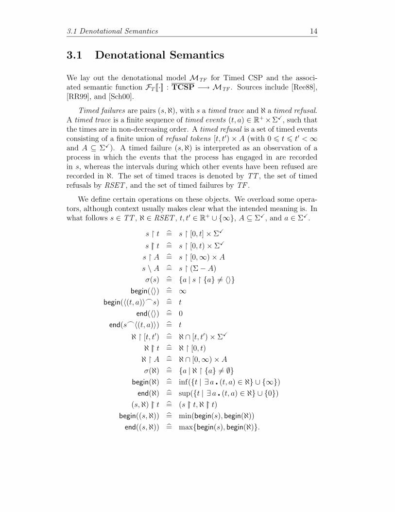
Timed failures are pairs (s,ℵ), with s a timed trace and ℵ a timed refusal.A timed trace is a finite sequence of timed events (t, a) ∈ R+×ΣX, such thatthe times are in non-decreasing order. A timed refusal is a set of timed eventsconsisting of a finite union of refusal tokens [t, t′) × A (with 0 6 t 6 t′ < ∞and A ⊆ ΣX). A timed failure (s,ℵ) is interpreted as an observation of aprocess in which the events that the process has engaged in are recordedin s, whereas the intervals during which other events have been refused arerecorded in ℵ. The set of timed traces is denoted by TT , the set of timedrefusals by RSET , and the set of timed failures by TF .
We define certain operations on these objects. We overload some opera-tors, although context usually makes clear what the intended meaning is. Inwhat follows s ∈ TT , ℵ ∈ RSET , t, t′ ∈ R+ ∪ {∞}, A ⊆ ΣX, and a ∈ ΣX.
s � t = s � [0, t] × ΣX
s |� t = s � [0, t) × ΣX
s � A = s � [0,∞) × A
s \ A = s � (Σ − A)
σ(s) = {a | s � {a} 6= 〈〉}
begin(〈〉) = ∞
begin(〈(t, a)〉_s) = t
end(〈〉) = 0
end(s_〈(t, a)〉) = t
ℵ � [t, t′) = ℵ ∩ [t, t′) × ΣX
ℵ |� t = ℵ � [0, t)
ℵ � A = ℵ ∩ [0,∞) × A
σ(ℵ) = {a | ℵ � {a} 6= ∅}
begin(ℵ) = inf({t | ∃ a � (t, a) ∈ ℵ} ∪ {∞})
end(ℵ) = sup({t | ∃ a � (t, a) ∈ ℵ} ∪ {0})
(s,ℵ) |� t = (s |� t,ℵ |� t)
begin((s,ℵ)) = min(begin(s), begin(ℵ))
end((s,ℵ)) = max{begin(s), begin(ℵ)}.

3.1 Denotational Semantics 15
We also define the information ordering ≺ on timed failures as follows:(s′,ℵ′) ≺ (s,ℵ) if there exists s′′ ∈ TT such that s = s′_s′′ and ℵ′ ⊆ ℵ |�begin(s′′).
Definition 3.1 The timed failures model MTF is the set of all P ⊆ TFsatisfying the following axioms, where s, s′ ∈ TT, ℵ,ℵ′ ∈ RSET, a ∈ ΣX,and t, u ∈ R+.
TF1 (〈〉, ∅) ∈ P
TF2 ((s,ℵ) ∈ P ∧ (s′,ℵ′) ≺ (s,ℵ)) ⇒ (s′,ℵ′) ∈ P
TF3 ((s,ℵ) ∈ P ∧ u > 0) ⇒
∃ℵ′ ∈ RSET � ℵ ⊆ ℵ′ ∧ (s,ℵ′) ∈ P ∧ ∀(t, a) ∈ [0, u) × ΣX�
((t, a) /∈ ℵ′ ⇒ (s � t_〈(t, a)〉,ℵ′ |� t) ∈ P ) ∧
((t > 0 ∧ @ ε > 0 � [t − ε, t) × {a} ⊆ ℵ′) ⇒
(s |� t_〈(t, a)〉,ℵ′ |� t) ∈ P )
TF4 ∀ t > 0 � ∃n ∈ N � ((s,ℵ) ∈ P ∧ end(s) 6 t) ⇒ ](s) 6 n
TF5 (s_〈(t,X)〉_s′,ℵ) ∈ P ⇒ s′ = 〈〉.
These axioms have the following intuitive interpretations:
TF1 : The least we can observe about a process is that it has communicatedno events and refused none.
TF2 : Any observation could have been replaced by another observation con-taining less information.
TF3 : Tells us how observations can be extended, and postulates the existenceof complete behaviours up to time u (for any u), which are maximalobservations under the information ordering ≺. Specifically, this axiomsays that any event not refusable at a certain time could have beenperformed at that time (albeit possibly only ‘after’ a number of eventsalso occurring at that precise time); however, if the event in questionwas not refusable over some interval, however small, leading to the timein question, then that event could have been the ‘first’ to occur at thattime. The fact that complete behaviours always exist also indicates thatany behaviour can be extended to one in which no event is infinitelyrepeatedly offered and withdrawn over a finite period of time, sincerefusals are finite unions of refusal tokens.

3.1 Denotational Semantics 16
TF4 : A process cannot perform infinitely many events in a finite time. Thisaxiom (known as finite variability) precludes such anomalies as Zenoprocesses.
TF5 : Stipulates that a process which has terminated may not communicateany further.
Note that Axiom TF3 implies that processes (can be observed to) runindefinitely. In other words, MTF processes cannot exhibit timestops.
We will return to these axioms later on when building our discrete-timemodels and compare them to their discrete-time counterparts.
We now list a few more definitions before presenting the denotationalmapping FT J·K.
For s = 〈(t1, a1), (t2, a2), . . . , (tk, ak)〉 and t > −begin(s) = −t1, we lets + t = 〈(t1 + t, a1), (t2 + t, a2), . . . , (tk + t, ak)〉. (Of course, s − t meanss + (−t)). For any t ∈ R, define ℵ + t = {(t′ + t, a) | (t′, a) ∈ ℵ ∧ t′ > −t}.Lastly, if t > −begin(s), then (s,ℵ) + t = (s + t,ℵ + t).
Given B ⊆ ΣX, we define an untimed merging operator (·) ‖B
(·) : TT ×
TT −→ P((R+ × ΣX)?), en route to defining an adequate parallel operatoron timed traces. In what follows, s ∈ (R+×ΣX)?, s1, s2, s
′1, s
′2 ∈ TT , t ∈ R+,
and a ∈ ΣX.
〈〉 ∈ s1 ‖B
s2 ⇔ s1 = s2 = 〈〉
〈(t, a)〉_s ∈ s1 ‖B
s2 ⇔ (a ∈ B ∧ s1 = 〈(t, a)〉_s′1 ∧
s2 = 〈(t, a)〉_s′2 ∧ s ∈ s′1 ‖B
s′2) ∨
(a /∈ B ∧ s1 = 〈(t, a)〉_s′1 ∧ s ∈ s′1 ‖B
s2) ∨
(a /∈ B ∧ s2 = 〈(t, a)〉_s′2 ∧ s ∈ s1 ‖B
s′2).
We now define (·) ‖B
(·) : TT × TT −→ P(TT ) by imposing the proper
ordering on timed events, and throwing out traces which fail to satisfy Ax-iom TF5. The notation is as above.
s ∈ s1 ‖B
s2 ⇔ s ∈ s1 ‖B
s2 ∧ s ∈ TT ∧ (s = s′_〈(t,X)〉_s′′ ⇒ s′′ = 〈〉).
We let s1 9 s2 = s1 ‖∅
s2, for any s1, s2 ∈ TT .

3.1 Denotational Semantics 17
A renaming function f : Σ −→ Σ has an obvious extension to timedtraces and timed refusals: if s = 〈(t1, a1), (t2, a2), . . . , (tk, ak)〉 ∈ TT andℵ ∈ RSET , then f(s) = 〈(t1, f(a1)), (t2, f(a2)), . . . , (tk, f(ak))〉, f(ℵ) ={(t, f(a)) | (t, a) ∈ ℵ}, and f−1(ℵ) = {(t, a) | (t, f(a)) ∈ ℵ}. Here f isextended to ΣX by setting f(X) = X.
The lambda abstraction λx.F (x) formally represents the function F . Forexample, λx.(x2+3) denotes the function F such that, for all x, F (x) = x2+3.
A semantic binding is a function ρ : VAR −→ MTF . Given a semanticbinding ρ and a process P ∈ MTF , we write ρ[X := P ] to denote a furthersemantic binding that is the same as ρ except that it returns P for X insteadof ρ(X). Naturally, if x is a variable ranging over MTF (i.e., x is a bonafide variable, not an element of VAR!), λx.ρ[X := x] represents a functionwhich, when fed an element P of MTF , returns a semantic binding (one thatis identical to ρ but for mapping X to P ).
If F : MTF −→ MTF has a unique fixed point, we denote it by fix(F ).(P ∈ MTF is a fixed point of F if F (P ) = P .)
We now define the function FT J·K inductively over the structure of TimedCSP terms. Since a term P ∈ TCSP may contain free variables, we alsorequire a semantic binding ρ in order to assign MTF processes to the freevariables of P .1 In what follows, s, s1, s2 ∈ TT , ℵ,ℵ1,ℵ2 ∈ RSET , t ∈ R+,a ∈ Σ, A ⊆ Σ, and B ⊆ ΣX. The rules are as follows:
FT JSTOPKρ = {(〈〉,ℵ)}
FT JSKIPKρ = {(〈〉,ℵ) |X /∈ σ(ℵ)}∪
{(〈(t,X)〉,ℵ) | t > 0 ∧ X /∈ σ(ℵ |� t)}
FT JWAIT nKρ = {(〈〉,ℵ) |X /∈ σ(ℵ � [n,∞))}∪
{(〈(t,X)〉,ℵ) | t > n ∧ X /∈ σ(ℵ � [n, t))}
FT JP1
n� P2Kρ = {(s,ℵ) | begin(s) 6 n ∧ (s,ℵ) ∈ FT JP1Kρ}∪
{(s,ℵ) | begin(s) > n ∧ (〈〉,ℵ |� n) ∈ FT JP1Kρ ∧
(s,ℵ) − t ∈ FT JP2Kρ}
1In reality, we are actually defining FT : TCSP × BIND −→ MTF , where BIND
stands for the set of all semantic bindings. Since our interest ultimately lies exclusivelyin the subset TCSP of TCSP (in which case the choice of semantic binding becomesirrelevant), we shall not be overly concerned with this point.

3.1 Denotational Semantics 18
FT Ja −→ P Kρ = {(〈〉,ℵ) | a /∈ σ(ℵ)}∪
{(〈(t, a)〉_s,ℵ) | t > 0 ∧ a /∈ σ(ℵ |� t) ∧
begin(s) > t ∧ (s,ℵ) − t ∈ FT JP Kρ}
FT Ja : A −→ P (a)Kρ = {(〈〉,ℵ) | A ∩ σ(ℵ) = ∅}∪
{(〈(t, a)〉_s,ℵ) | a ∈ A ∧ t > 0 ∧
A ∩ σ(ℵ |� t) = ∅ ∧ begin(s) > t ∧
(s,ℵ) − t ∈ FT JP (a)Kρ}
FT JP1 2 P2Kρ = {(〈〉,ℵ) | (〈〉,ℵ) ∈ FT JP1Kρ ∩ FT JP2Kρ}∪
{(s,ℵ) | s 6= 〈〉 ∧ (s,ℵ) ∈ FT JP1Kρ ∪ FT JP2Kρ ∧
(〈〉,ℵ |� begin(s)) ∈ FT JP1Kρ ∩ FT JP2Kρ}
FT JP1 u P2Kρ = FT JP1Kρ ∪ FT JP2Kρ
FT JP1 ‖B
P2Kρ = {(s,ℵ) | ∃ s1, s2,ℵ1,ℵ2 � s ∈ s1 ‖B
s2 ∧
ℵ1 � (Σ − B) = ℵ2 � (Σ − B) = ℵ � (Σ − B) ∧
ℵ1 � B ∪ ℵ2 � B = ℵ � B ∧
(s1,ℵ1 |� begin(s � {X})) ∈ FT JP1Kρ ∧
(s2,ℵ2 |� begin(s � {X})) ∈ FT JP2Kρ}
FT JP1 9 P2Kρ = {(s,ℵ) | ∃ s1, s2 � s ∈ s1 9 s2 ∧
(s1,ℵ |� begin(s � {X})) ∈ FT JP1Kρ ∧
(s2,ℵ |� begin(s � {X})) ∈ FT JP2Kρ}
FT JP1 ; P2Kρ = {(s,ℵ) |X /∈ σ(s) ∧
(s,ℵ ∪ ([0, end((s,ℵ))) × {X})) ∈ FT JP1Kρ}∪
{(s1_s2,ℵ) |X /∈ σ(s1) ∧ (s2,ℵ) − t ∈ FT JP2Kρ ∧
(s1_〈(t,X)〉,ℵ |� t ∪ ([0, t) × {X})) ∈ FT JP1Kρ}
FT JP \ AKρ = {(s \ A,ℵ) | (s,ℵ ∪ ([0, end((s,ℵ))) × A)) ∈ FT JP Kρ}
FT Jf−1(P )Kρ = {(s,ℵ) | (f(s), f(ℵ)) ∈ FT JP Kρ}
FT Jf(P )Kρ = {(f(s),ℵ) | (s, f−1(ℵ)) ∈ FT JP Kρ}
FT JXKρ = ρ(X)
FT JµX � P Kρ = fix(λx.FT JP K(ρ[X := x])).
The following results are due to Reed [Ree88].
Proposition 3.1 Well-definedness: for any term P , and any semantic bind-ing ρ, FT JP Kρ ∈ MTF .

3.2 Operational Semantics 19
Proposition 3.2 If P is a Timed CSP program (i.e., P ∈ TCSP), then,for any semantic bindings ρ and ρ′, FT JP Kρ = FT JP Kρ′.
We will henceforth drop mention of semantic bindings when calculatingthe semantics of programs.
3.2 Operational Semantics
The contents and style of this section derive essentially from [Sch95]. Wepresent a collection of inference rules with the help of which any TCSP pro-gram can be assigned a unique labelled transition system, or LTS . Such LTS’sare the operational counterparts of denotational process representations. Afuller and more formal discussion of operational semantics (especially in CSPcontexts) can be found in [Ros97].
An operational semantics can usually ascribe behaviours to programs thatare not necessarily well-timed; moreover, because it is state-based, we mustequip it with a means to describe intermediate computational states whichin certain cases TCSP notation is unable to do. For this reason, we willconsider terms generated by the following less restrictive grammar:
P := STOP | SKIP | WAIT t | P1
t� P2 |
a −→ P | a : A −→ P (a) | P1 2 P2 | P1 u P2 |
P1 ‖B
P2 | P1 9 P2 | P1 ; P2 | P \ A |
f−1(P ) | f(P ) | X | µX � P.
Here t can be any non-negative real number, and we have dropped anyrequirement of well-timedness.2 The remainder of our conventions aboutTimed CSP syntax (see Section 2.1) however apply. We denote the set ofterms which this grammar generates by NODETF and the set of closed terms(not containing free variables) by NODETF , dropping the subscripts whenno confusion is likely. Elements of NODE are called (open) nodes whereaselements of NODE are called (closed) nodes. We insist that our inference
2Forgoing well-timedness is not absolutely necessary, but does no harm and certainlygreatly simplifies matters in the presence of fractional delays; in addition, we will see lateron why it is convenient to be able to write certain specifications in terms of non-well-timednodes.

3.2 Operational Semantics 20
rules only apply to closed nodes. Note that TCSP ⊆ NODE and TCSP ⊆NODE .
We list a few notational conventions: a and b stand for (non-tock) visibleevents, i.e., belong to ΣX. A ⊆ Σ and B ⊆ ΣX. µ can be a visible event
or a silent one (µ ∈ ΣX ∪ {τ}). Pµ
−→ P ′ means that the closed node Pcan perform an immediate and instantaneous µ-transition, and become the
closed node P ′ (communicating µ in the process if µ is a visible event). Pµ
X−→
means that P cannot possibly do a µ at that particular time. Pt P ′ means
that P can become P ′ simply by virtue of letting t units of time elapse, wheret is a non-negative real number. If P and Q are open nodes and X ∈ VAR,P [Q/X] represents the node P with Q substituted for every free occurrenceof X.
The inference rules take the general form
antecedent(s)
conclusion[ side condition ]
where either antecedents or side condition, or both, can be absent. (Theside condition is an antecedent typically dealing with matters other thantransitions or evolutions.) The rules are as follows.
STOPt STOP
(3.1)
SKIPt SKIP
(3.2)
SKIPX
−→ STOP(3.3)
WAIT ut WAIT (u − t)
[ t 6 u ] (3.4)
WAIT 0τ
−→ SKIP(3.5)

3.2 Operational Semantics 21
P1t P ′
1
P1
u� P2
t P ′
1
u−t� P2
[ t 6 u ] (3.6)
P1
0� P2
τ−→ P2
(3.7)
P1τ
−→ P ′1
P1
u� P2
τ−→ P ′
1
u� P2
(3.8)
P1a
−→ P ′1
P1
u� P2
a−→ P ′
1
(3.9)
(a −→ P )t (a −→ P )
(3.10)
(a −→ P )a
−→ P(3.11)
(a : A −→ P (a))t (a : A −→ P (a))
(3.12)
(a : A −→ P (a))b
−→ P (b)[ b ∈ A ] (3.13)
P1t P ′
1 P2t P ′
2
P1 2 P2t P ′
1 2 P ′2
(3.14)
P1τ
−→ P ′1
P1 2 P2τ
−→ P ′1 2 P2
P2τ
−→ P ′2
P1 2 P2τ
−→ P1 2 P ′2
(3.15)

3.2 Operational Semantics 22
P1a
−→ P ′1
P1 2 P2a
−→ P ′1
P2a
−→ P ′2
P1 2 P2a
−→ P ′2
(3.16)
P1 u P2τ
−→ P1 P1 u P2τ
−→ P2
(3.17)
P1t P ′
1 P2t P ′
2
P1 ‖B
P2t P ′
1 ‖B
P ′2
(3.18)
P1µ
−→ P ′1
P1 ‖B
P2µ
−→ P ′1 ‖
B
P2
[ µ /∈ B, µ 6= X ] (3.19a)
P2µ
−→ P ′2
P1 ‖B
P2µ
−→ P1 ‖B
P ′2
[ µ /∈ B, µ 6= X ] (3.19b)
P1a
−→ P ′1 P2
a−→ P ′
2
P1 ‖B
P2a
−→ P ′1 ‖
B
P ′2
[ a ∈ B ] (3.20)
P1X
−→ P ′1
P1 ‖B
P2X
−→ P ′1
[X /∈ B ]P2
X−→ P ′
2
P1 ‖B
P2X
−→ P ′2
[X /∈ B ] (3.21)
P1t P ′
1 P2t P ′
2
P1 9 P2t P ′
1 9 P ′2
(3.22)
P1µ
−→ P ′1
P1 9 P2µ
−→ P ′1 9 P2
[ µ 6= X ] (3.23a)
P2µ
−→ P ′2
P1 9 P2µ
−→ P1 9 P ′2
[ µ 6= X ] (3.23b)

3.2 Operational Semantics 23
P1X
−→ P ′1
P1 9 P2X
−→ P ′1
P2X
−→ P ′2
P1 9 P2X
−→ P ′2
(3.24)
P1t P ′
1 P1X
X−→
P1 ; P2t P ′
1 ; P2
(3.25)
P1X
−→ P ′1
P1 ; P2τ
−→ P2
(3.26)
P1µ
−→ P ′1
P1 ; P2µ
−→ P ′1 ; P2
[ µ 6= X ] (3.27)
Pt P ′ ∀ a ∈ A � P
aX−→
P \ At P ′ \ A
(3.28)
Pa
−→ P ′
P \ Aτ
−→ P ′ \ A[ a ∈ A ] (3.29)
Pµ
−→ P ′
P \ Aµ
−→ P ′ \ A[ µ /∈ A ] (3.30)
Pt P ′
f−1(P )t f−1(P ′)
(3.31)
Pµ
−→ P ′
f−1(P )µ
−→ f−1(P ′)[ µ ∈ {τ,X} ] (3.32)
Pf(a)−→ P ′
f−1(P )a
−→ f−1(P ′)(3.33)

3.2 Operational Semantics 24
Pt P ′
f(P )t f(P ′)
(3.34)
Pµ
−→ P ′
f(P )µ
−→ f(P ′)[ µ ∈ {τ,X} ] (3.35)
Pa
−→ P ′
f(P )f(a)−→ f(P ′)
(3.36)
µX � Pτ
−→ P [(µX � P )/X].(3.37)
The reader may have noticed that Rules 3.25 and 3.28 incorporate nega-
tive premisses (P1X
X−→ and Pa
X−→), which could potentially yield an inconsis-tent definition. This does not occur, for the following reason: notice that the
x−→ relation can be defined, independently of the
t relation, as the smallest
relation satisfying the relevant subset of rules, since no negative premissesare involved in its definition. Once the
x−→ relation has been defined, the
t relation can then itself be defined. Since the negative premisses are allphrased in terms of the previously defined (and fixed)
x−→ relation, they do
not pose any problem.
We now present a number of results about the operational semantics. Webegin with some definitions.
If P and Q are open nodes, we write P ≡ Q to indicate that P and Qare syntactically identical.
If P is a closed node, we define initτTF
(P ) to be the set of visible and silent
events that P can immediately perform: initτTF
(P ) = {µ | Pµ
−→}. We alsowrite initTF (P ) to represent the set of visible events that P can immediatelyperform: initTF (P ) = initτ
TF(P ) ∩ ΣX. We will usually write initτ (P ) and
init(P ) for short when no confusion is likely.
For P a closed node, we define an execution of P to be a sequence e =P0
z17−→ P1z27−→ . . .
zn7−→ Pn (with n > 0), where P0 ≡ P , the Pi’s are nodes,
and each subsequence Pi
zi+17−→ Pi+1 in e is either a transition Pi
µ−→ Pi+1 (with

3.2 Operational Semantics 25
zi+1 = µ), or an evolution Pit Pi+1 (with zi+1 = t). In addition, every such
transition or evolution must be validly allowed by the operational inferenceRules 3.1–3.37. The set of executions of P is written execTF (P ), or exec(P )for short when no confusion with notation introduced later on is likely. Byconvention, writing down a transition (or sequence thereof) such as P
a−→ P ′
is equivalent to stating that Pa
−→ P ′ ∈ exec(P ); the same, naturally, goesfor evolutions.
For P a closed node, the P -rooted graph, or labelled transition system,incorporating all of P ’s possible executions is denoted LTSTF (P ), or LTS(P )if no confusion is likely.
Every execution e gives rise to a timed τ -trace abs(e) in the obvious way,by removing nodes and evolutions from the execution, but recording events’time of occurrence in agreement with e’s evolutions. (A timed τ -trace is atimed trace over ΣX ∪ {τ}.) The formal inductive definition of abs is asfollows:
abs(P ) = 〈〉
abs((Pµ
−→)_e) = 〈(0, µ)〉_abs(e)
abs((Pt )_e) = abs(e) + t.
The duration of an evolution e is equal to the sum of its evolutions:dur(e) = end(abs(e)).
We then have the following results, adapted from [Sch95]. (Here P, P ′, P ′′
are closed nodes, t, t′ are non-negative real numbers, etc.).
Proposition 3.3 Time determinacy:
(Pt P ′ ∧ P
t P ′′) ⇒ P ′ ≡ P ′′.
Proposition 3.4 Persistency—the set of possible initial visible events re-mains constant under evolution:
Pt P ′ ⇒ init(P ) = init(P ′).
Proposition 3.5 Time continuity:
Pt+t′
P ′ ⇔ ∃P ′′ � Pt P ′′ t′
P ′.
3.2 Operational Semantics 26
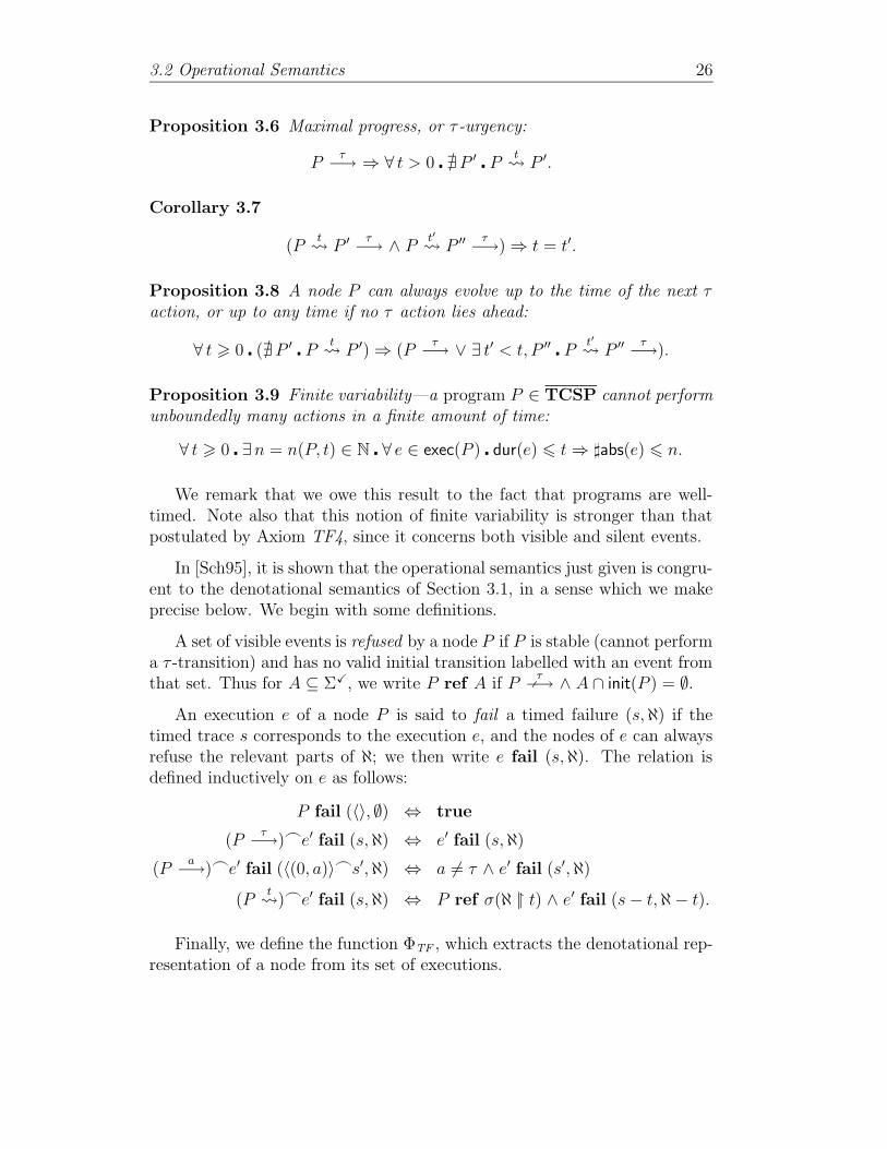
Proposition 3.6 Maximal progress, or τ -urgency:
Pτ
−→ ⇒ ∀ t > 0 � @ P ′ � Pt P ′.
Corollary 3.7
(Pt P ′ τ
−→ ∧ Pt′
P ′′ τ−→) ⇒ t = t′.
Proposition 3.8 A node P can always evolve up to the time of the next τaction, or up to any time if no τ action lies ahead:
∀ t > 0 � (@ P ′ � Pt P ′) ⇒ (P
τ−→ ∨ ∃ t′ < t, P ′′ � P
t′
P ′′ τ−→).
Proposition 3.9 Finite variability—a program P ∈ TCSP cannot performunboundedly many actions in a finite amount of time:
∀ t > 0 � ∃n = n(P, t) ∈ N � ∀ e ∈ exec(P ) � dur(e) 6 t ⇒ ]abs(e) 6 n.
We remark that we owe this result to the fact that programs are well-timed. Note also that this notion of finite variability is stronger than thatpostulated by Axiom TF4, since it concerns both visible and silent events.
In [Sch95], it is shown that the operational semantics just given is congru-ent to the denotational semantics of Section 3.1, in a sense which we makeprecise below. We begin with some definitions.
A set of visible events is refused by a node P if P is stable (cannot performa τ -transition) and has no valid initial transition labelled with an event fromthat set. Thus for A ⊆ ΣX, we write P ref A if P
τX−→ ∧ A ∩ init(P ) = ∅.
An execution e of a node P is said to fail a timed failure (s,ℵ) if thetimed trace s corresponds to the execution e, and the nodes of e can alwaysrefuse the relevant parts of ℵ; we then write e fail (s,ℵ). The relation isdefined inductively on e as follows:
P fail (〈〉, ∅) ⇔ true
(Pτ
−→)_e′ fail (s,ℵ) ⇔ e′ fail (s,ℵ)
(Pa
−→)_e′ fail (〈(0, a)〉_s′,ℵ) ⇔ a 6= τ ∧ e′ fail (s′,ℵ)
(Pt )_e′ fail (s,ℵ) ⇔ P ref σ(ℵ |� t) ∧ e′ fail (s − t,ℵ − t).
Finally, we define the function ΦTF , which extracts the denotational rep-resentation of a node from its set of executions.

3.3 The Digitisation Lemma 27
Definition 3.2 For P ∈ NODE, we set
ΦTF (P ) = {(s,ℵ) | ∃ e ∈ execTF (P ) � e fail (s,ℵ)}.
We can now state the chief congruence result:
Theorem 3.10 For any TCSP program P , we have
ΦTF (P ) = FT JP K.
3.3 The Digitisation Lemma
The single result of this section, which we call the digitisation lemma, willenable us to relate this chapter’s continuous-time semantics for Timed CSPto the discrete-time semantics introduced in Chapters 5 and 7. We first needa small piece of notation. Let t ∈ R+, and let 0 6 ε 6 1 be a real number.Decompose t into its integral and fractional parts, thus: t = btc+ t. (Here btcrepresents the greatest integer less than or equal to t.) If t < ε, let [t]ε = btc,otherwise let [t]ε = dte. (Naturally, dte denotes the least integer greater thanor equal to t.) The [·]ε operator therefore shifts the value of a real numbert to the preceding or following integer, depending on whether the fractionalpart of t is less than the ‘pivot’ ε or not.
Lemma 3.11 Let P ∈ TCSP, and let e = P0z17−→ P1
z27−→ . . .zn7−→ Pn ∈
execTF (P ). For any 0 6 ε 6 1, there exists an execution [e]ε = P ′0
z′17−→
P ′1
z′27−→ . . .z′n7−→ P ′
n ∈ execTF (P ) with the following properties:
1. The transitions and evolutions of e and [e]ε are in natural one-to-one
correspondence. More precisely, whenever Pi
zi+17−→ Pi+1 in e is a tran-
sition, then so is P ′i
z′i+17−→ P ′
i+1 in [e]ε, and moreover z′i+1 = zi+1. On
the other hand, whenever Pi
zi+17−→ Pi+1 in e is an evolution, then so is
P ′i
z′i+17−→ P ′
i+1 in [e]ε, with |zi+1 − z′i+1| < 1.
2. All evolutions in [e]ε have integral duration.
3. P ′0 ≡ P0 ≡ P ; in addition, P ′
i ∈ TCSP and initTF (P ′i ) = initTF (Pi) for
all 0 6 i 6 n.

3.4 Refinement, Specification, Verification 28
4. For any prefix e(k) = P0z17−→ P1
z27−→ . . .zk7−→ Pk of e, the corresponding
prefix [e]ε(k) of [e]ε is such that dur([e]ε(k)) = [dur(e(k))]ε.
Executions all of whose evolutions have integral duration are called inte-gral executions. The integral execution [e]ε as constructed above is called theε-digitisation of e.3 The special case ε = 1 is particularly important: eachtransition in [e]1 happens at the greatest integer time less than or equal tothe time of occurrence of its vis-a-vis in e; for this reason [e]1 is termed thelower digitisation of e.
Proof (Sketch.) The proof proceeds by structural induction over TimedCSP syntax. Among the tools it introduces and makes substantial use offigures the notion of indexed bisimulation. It is interesting to note that thecrucial property of P required in the proof is the fact that all delays in P areintegral; well-timedness is irrelevant. Details can be found in Appendix A.
�
3.4 Refinement, Specification, Verification
An important partial order can be defined on P(TF ), as follows:
Definition 3.3 For P,Q ⊆ TF (and in particular for P,Q ∈ MTF ), welet P vTF Q if P ⊇ Q. For P,Q ∈ TCSP, we write P vTF Q to meanFT JP K vTF FT JQK, and P =TF Q to mean FT JP K = FT JQK.
We may drop the subscripts and write simply P v Q, P = Q whenever thecontext is clear.
This order, known as timed failure refinement, has the following centralproperty (as can be verified by inspection of the relevant definitions). HereP and Q are processes:
P v Q ⇔ P u Q = P. (3.38)
For this reason, v is also referred to as the order of nondeterminism—P v Qif and only if P is ‘less deterministic’ than Q, or in other words if and onlyif Q’s behaviour is more predictable (in a given environment) than P ’s.
3Although [e]ε is not necessarily unique for a given execution e, we consider any twosuch executions to be interchangeable for our purposes.
3.4 Refinement, Specification, Verification 29
Similar refinement orders (all obeying Equation (3.38) above) can be de-fined in most other (timed and untimed) CSP models. These orders areoften of significantly greater importance in untimed models as they consti-tute the basis for the computation of fixed points (whereas timed models areusually predicated upon ultrametric spaces which rely on a different fixed-point theory). Refinement orders also play a central role as specificationformalisms within untimed or discrete-time CSP models, whereas they canprove problematic for that purpose in dense timed models (as we demonstratebelow). Nonetheless, because this work specifically studies the relationshipbetween discrete and continuous modelling paradigms for timed systems, itis imperative to include refinement in our investigations. In addition, sinceP = Q ⇔ (P v Q ∧ Q v P ), a decision procedure for refinement yields adecision procedure for process equivalence, a central and perennial problemin Computer Science. (Incidentally, the converse—deciding refinement fromprocess equivalence—follows from Equation (3.38).)
For P ⊆ TF , let TTraces(P ) be the set of timed traces of P . Using this,we define a second notion of refinement—timed trace refinement—betweensets of timed failures (and in particular MTF processes):
Definition 3.4 For any P,Q ⊆ TF, we let P vTT Q if TTraces(P ) ⊇TTraces(Q).
We overload the notation and extend vTT to TCSP programs in the obviousway.
A major aim of the field of process algebra is to model systems so as tobe able to formulate and establish assertions concerning them. Such asser-tions are usually termed specifications. Depending upon the model underconsideration, specifications can take wide-ranging forms. Our principal in-terest in this thesis concerns denotational models, and accordingly we willdeal exclusively with specifications expressed in terms of these models.
In general, a specification S = S(P ) on processes is simply a predicateon P ; for example it could be S(P ): ‘P cannot perform any events’. Thiscan be expressed in English (as we have done here), mathematically ((s,ℵ) ∈P ⇒ s = 〈〉), refinement-theoretically (STOP vTT P or STOP vTF P ), orusing some other formalism such as temporal logic4. All these formulationsare easily seen to be equivalent over MTF , and in this work we shall not
4An excellent account of the use of temporal logic(s) as a specification formalism inboth Timed and untimed CSP can be found in [Jac92].

3.4 Refinement, Specification, Verification 30
be overly concerned with the particular formalism chosen. We do remark,however, that expressing specifications in terms of refinement can lead toproblematic situations. For instance, one would naturally want to express thespecification S(P ): ‘P cannot perform the event a’ as RUN ΣX−{a} vTT P ,where RUN A = a : A −→ RUN A. The problem is that RUN A is not awell-timed process, and even if, as we have seen, it can easily be modelled inan operational semantics, no-one has yet produced a consistent denotationalmodel in which such Zeno processes could be interpreted.5
Note that even models allowing unbounded nondeterminism (see, e.g.,[MRS95]) place restrictions disallowing, among others, an internal choiceover the set of processes unable to perform an a. The attempt to expressS(P ) asu{Q ∈ TCSP| ∀ s ∈ TTraces(FT JQK)�a /∈ σ(s)} vTF P is thereforealso doomed.
Thus while in practice one could conceivably still express, for a givenprocess P , the desired specification as a refinement between P and a well-timed process, this example shows that one cannot rigorously do so on ageneral basis. We shall return to this question later on.
A process P meets, or satisfies, a specification S, if S(P ) is true; in thatcase we write P � S.
Specifications fall naturally into certain categories. A timed trace specifi-cation, for example, is one that can be stated exclusively in terms of timedtraces. We are particularly (though not exclusively) interested in a type ofspecifications known as behavioural specifications. A behavioural specifica-tion is one that is universally quantified over the behaviours of processes. Inother words, S = S(P ) is a behavioural specification if there is a predicateS ′(s,ℵ) on timed failures such that, for any P ,
P � S ⇔ ∀(s,ℵ) ∈ P � S ′(s,ℵ).
In this case we may abuse notation and identify S with S ′. Note that S ′
itself may be identified with a subset of TF , namely the set of (s,ℵ) ∈ TFsuch that S ′(s,ℵ).
A safety property is a requirement that ‘nothing bad happen’. For usthis will translate as a behavioural timed trace specification: certain timedtraces are prohibited.6 A liveness property is one that says ‘something good
5Aside from finite variability, the dual requirement that refusals should consist in fi-
nite unions of left-closed, right-open intervals makes embedding MTF into a domain achallenging problem. Contrast this with our discussion on the same topic in Section 5.3.
6It can be argued that certain specifications, which cannot be expressed entirely interms of timed traces, are in fact safety properties, but we will for simplicity nonetheless

3.4 Refinement, Specification, Verification 31
is not prevented from happening’. Thus a liveness property in general simplycorresponds to a behavioural timed failure specification, although in practicewe expect such a specification to primarily concern refusals.
Any specification S = S(P ) which can be expressed, for a fixed processQ, as Q v P , is automatically behavioural. (Note that the reverse refine-ment, P v Q, is not.) Thus behavioural specifications are identified withrequirements : the implementation (P ) must have all the safety and livenessproperties of the requirement (Q).
The discussion in the remainder of this section concerns behavioural spec-ifications exclusively.
A number of techniques have been devised to help decide when a givenTimed CSP process meets a particular specification. Schneider [Sch89] andDavies [Dav91] have produced complete proof systems, sets of rules enablingone to derive specification satisfaction, for various models of Timed CSP. Acase study illustrating the use of such proof systems is presented in [Sch94].These techniques, along with an impressive array of related methodologies,however require significant prior insight before they can be reasonably appliedto particular problems, and do not appear likely to be mechanisable in theirpresent form.
Another technique is that of timewise refinement, introduced by Reedin [Ree88, Ree89] and developed by Schneider in [Sch89, RRS91, Sch97]. Itcan sometimes be used to establish certain untimed properties of timed pro-cesses, by removing all timing information from them, and verifying that thecorresponding (untimed) CSP processes exhibits the properties in question.Simple criteria exist to decide when this technique can be soundly applied. Itis clearly mechanisable (since the verification of (untimed) CSP processes it-self is), but suffers from obvious restrictions in its applicability. Nonetheless,it can prove enormously useful in those cases where it can be employed.
A third approach was taken by Jackson in [Jac92], in which he devel-ops full-fledged temporal-logic-based specification languages, and, invokingthe seminal region graphs methods of Alur, Courcoubetis, and Dill [ACD90,ACD93], shows how a restricted subset of Timed CSP yields processes forwhich the verification of certain temporal logic specifications can always a pri-ori be model checked. His restrictions on Timed CSP ensure that processesremain, in a certain sense, finite state. He then translates such processes intotimed graphs, and constructs an equivalence relation which identifies statesthat essentially cannot be distinguished by the clocks at hand. This yields a
stick with the proposed terminology in this work.
3.4 Refinement, Specification, Verification 32
finite quotient space which can then be mechanically explored. Some currentdisadvantages of this technique are the sharp syntactic restrictions it imposeson Timed CSP, as well as the constraints on the sort of specifications whichare allowable (excluding, for instance, refinement checks). It should be addedthat the complexity of the resulting model checking algorithm is quite high;we shall return to this point in Chapter 9.

Chapter 4
Discrete-Time Modelling:Motivation
In this chapter, we aim to provide the intuition behind the constructions ofthe discrete-time models presented in Chapters 5 and 7. We will look at eachof the Timed CSP operators in turn, and discuss how best to interpret themwithin a CSP-based discrete-time framework. We assume some familiaritywith the standard CSP semantics ([Ros97, Sch00] are two good references),which we will invoke throughout; however, the rest of this thesis is self-contained (with the exception of sections 5.4 and 6.7), so that this chaptermay be skipped with no significant loss of continuity.
We will define a ‘translation’ function Ψ converting Timed CSP syntaxinto CSP syntax, in such a way that the behaviours of Ψ(P ), interpretedin a CSP framework, approximate as closely as possible those of the TCSPprogram P , interpreted in the timed failures model. This translation, in otherwords, should preserve as much timing information as possible. (We will notlater explicitly require Ψ, nor any other of the constructs introduced in thischapter, except in sections 5.4 and 6.7, to describe how TCSP programs canbe model checked on the automated tool FDR.)
We define Ψ inductively over Timed CSP syntax in the following fewsections.
4.1 Event Prefixing 34
4.1 Event Prefixing
Consider the program Q = a −→ P . Interpreted in MTF , this process isinitially prepared to let time pass at will; there is no requirement for a tooccur within any time period. In standard CSP models, however, such aprocess is of course incapable of initially communicating any tocks, which wewould interpret as ‘forcing’ a to occur within at most one time unit.
An adequate translation of Q, therefore, has to ensure the unhinderedpassage of time, or in other words that tock events are always permissible.The desired new program, then, should be written: Q′ = (a −→ P ) 2
(tock −→ Q′). We abbreviate this construct as Q′ = a −→t P (where thesubscript ‘t’ stands for tock). In other words,
a −→t P = µX � ((a −→ P ) 2 (tock −→ X)).
Of course, P must also be suitably translated as the process makesprogress. We thus set, in general
Ψ(a −→ P ) = a −→t Ψ(P ).
Extending this to the case of the general prefix operator yields
Ψ(a : A −→ P (a)) = a : A −→t Ψ(P (a)).
4.2 Deadlock, Termination, Delay
Naturally, the treatment of STOP must follow a similar path: its interpre-tation in MTF allows time to pass at will. Hence
Ψ(STOP) = µX � tock −→ X = STOP t.
It should be equally clear how to handle SKIP :
Ψ(SKIP ) = X −→t STOP t = SKIP t.
As for WAIT n, a little thought reveals that
Ψ(WAIT n) =
n tocks︷ ︸︸ ︷tock −→ . . . −→ tock −→ SKIP t = WAIT t n
is the only reasonable proposal. Note, importantly, that this definition usesthe −→ operator (rather than −→t), so as to guarantee that a X be on offerafter exactly n tocks.

4.3 External Choice 35
4.3 External Choice
The program Q = P1 2 P2 poses some slightly more intricate problems. OverMTF , Q will wait however long it takes for either P1 or P2 to communicatea visible event, at which point the choice will be resolved in favour of thatprocess. Unfortunately, if tocks are interpreted as regular events, the choicewill ipso facto be made within at most one time unit under CSP semantics.
The solution is to postulate a new operator 2t that behaves like 2 inall respects, except that it lets tocks ‘seep through’ it without forcing thechoice to be resolved. Here we are assuming, in addition, that P1 and P2
synchronise on every tock communication, for reasons discussed in the nextsection.
Direct operational and denotational definitions of 2t can be given, butthe following construct (due to Steve Schneider) shows that 2t can in factbe expressed in terms of standard CSP operators, if we assume that P1 andP2 can never refuse tock :
First let Σ1 = {1.a | a ∈ Σ} and Σ2 = {2.a | a ∈ Σ}. Next, define twofunctions f1, f2 : Σtock ∪ Σ1 ∪ Σ2 −→ Σtock ∪ Σ1 ∪ Σ2 such that
fi(a) = i.a if a ∈ Σ= a otherwise.
Finally, we have
P1 2t P2 = f−11 (f−1
2 ((f1(P1) ‖{tock}
f2(P2)) ‖Σ1∪Σ2
(RUN Σ12 RUN Σ2
)))
where RUN A = a : A −→ RUN A.
Naturally, we set
Ψ(P1 2 P2) = Ψ(P1) 2t Ψ(P2).
Note, however, that in most cases a much simpler translation can beobtained: (a −→t P1) 2t (b −→t P2), for instance, is equivalent to Q =(tock −→ Q) 2 (a −→ P1) 2 (b −→ P2) in CSP models.
4.4 Concurrency
The main point concerning the parallel operators ‖B
and 9 is that they should
ensure a uniform rate of passage of time: no process in a parallel composition

4.5 Hiding and Sequential Composition 36
should be allowed to run ‘faster’ than another. This is achieved, naturally,by forcing processes to synchronise on tock . Thus
Ψ(P1 ‖B
P2) = Ψ(P1) ‖B∪{tock}
Ψ(P2) = Ψ(P1) ‖tB
Ψ(P2).
Since interleaving normally corresponds to parallel composition over anempty interface, we set
Ψ(P1 9 P2) = Ψ(P1) ‖{tock}
Ψ(P2) = Ψ(P ) 9t Ψ(Q).
4.5 Hiding and Sequential Composition
An adequate discrete-time treatment of hiding and sequential compositionpits us against greater difficulties than the other operators. This is a directconsequence of the assumption of maximal progress, or τ -urgency: hiddenevents must happen as quickly as possible.1
As an illustration, consider the program
P = ((a −→ STOP) 2 WAIT 1) ; b −→ STOP .
Interpreted over MTF , P initially offers the event a for exactly one time unit,after which (if a has not occurred) the offer is instantly withdrawn and anopen-ended offer of b is made. (This is one of the simplest possible examplesof a timeout.)
Unfortunately, the behaviours of
P ′ = ((a −→t STOP t) 2t (tock −→ SKIP t)) ; b −→t STOP t,
in CSP models, are easily seen to allow an a to be communicated afteran arbitrary number of tocks; this is because the hidden X, which SKIP t
can potentially communicate, is not made urgent by sequential composition,contrary to the situation with P in MTF . In other words, P ′ is not anadequate translation of P .
In order to faithfully capture, in a discrete-time setting, the timed be-haviours of hiding and sequential composition, it is necessary to postulate
1The reasons for requiring the maximal progress assumption (in the absence of whichit is impossible, for instance, to implement proper timeouts) are well-known and discussedin most expository texts on timed systems—see, for instance, [Sch00].

4.5 Hiding and Sequential Composition 37
the urgency of hidden events. By this we mean that the event tock shouldnot be allowable so long as a silent (τ) event is on offer.
Although it is easy to capture this requirement operationally (as we shallsee in Chapter 5), it is impossible to render it in either the traces or thefailures models, which are the main denotational models for CSP. (Tracesare sequences of events that a process can be observed to communicate,whereas a failure is trace augmented by a refusal at the end of the trace: arecord of events that the process cannot perform after the given trace.) Thefollowing example (originally due to Langerak [Lan90], and reproduced in[Sch00]) shows why failures are unable support τ -urgency in a compositionalway.
Consider the programs P and Q, defined in terms of TEA and COFFEE :
TEA = tea −→t STOP t
COFFEE = coffee −→t STOP t
P = TEA u COFFEE
Q = ((coffee −→ STOP t) 2 (tock −→ TEA)) u
((tea −→ STOP t) 2 (tock −→ COFFEE )).
P and Q have the same set of failures: they can both perform any numberof tocks followed by a tea or a coffee (followed by further tocks); and, at anystage before a drink is delivered, either tea or coffee, but not both, can berefused.
However, there is a difference in their behaviour: P is always committedto the drink it first chooses to offer, whereas after one tock Q switches thedrink it offers. Failure information is not detailed enough to identify thisdifference.
Nevertheless, this difference in behaviour means that, under τ -urgency,P \ tea can provide a coffee after a tock , whereas Q \ tea cannot—the hiddentea will occur either immediately or after one tock , in both cases preventingthe possibility of coffee after tock . Hence we conclude that, under τ -urgency,the failures alone of a process P are not sufficient to determine even thetraces of P \ A, let alone the failures.
The question then arises as how to capture τ -urgency denotationally. Itturns out that, although τ events are introduced by other operators besideshiding and sequential composition, it is sufficient to require urgent behaviourof hiding and sequential composition alone to ensure τ -urgency in general.

4.6 Timeout 38
Recall that behaviours of P \ A are derived from those of P . To guaranteeurgency, it is sufficient, in calculating the behaviours of P \ A, to dismissany behaviour of P in which a tock is recorded while events from the set Awere on offer. A similar proposal handles sequential composition.
In order to know whether events in A were refusable prior to an occurrenceof tock or not, one must record refusal information throughout a trace, ratherthan exclusively at the end of it. This type of modelling, known as refusaltesting, was introduced by Phillips [Phi87] and served as the basis for therefusal testing models of Mukarram [Muk93]. The denotational models wepresent in Chapter 5 and 7 are thus also refusal testing based.
As a reminder (especially when using an automated model checker) thatτ -urgency is required, we will use the symbols \t and ;t to represent respec-tively urgent hiding and urgent sequential composition within CSP. Thuswe set
Ψ(P \ A) = Ψ(P ) \t A
Ψ(P1 ; P2) = Ψ(P1) ;t Ψ(P2).
4.6 Timeout
The MTF behaviour of the timeout operator exhibits characteristics of bothexternal choice and sequential composition; the problems it presents cantherefore be tackled using techniques similar to those shown above. In prac-tice, assuming that the event trig does not figure in the alphabet of either P1
or P2, one has the identity P1
n� P2 = (P1 2 (WAIT n ; trig −→ P2)) \ trig ,
and thus
Ψ(P1
n� P2) = (Ψ(P1) 2t (WAIT t n ;t trig −→t Ψ(P2))) \t trig
= Ψ(P1)n�t Ψ(P2).
4.7 Others
The remaining operators, namely internal choice, renaming, and recursion,pose no difficulties: each is left unchanged. Naturally, the same goes forprogram variables. We recapitulate the full definition of Ψ after listing thenew constructs introduced in this chapter.

4.8 Summary 39
4.8 Summary
Definition 4.1 We have defined the following syntactic operators.
a −→t P = µX � ((a −→ P ) 2 (tock −→ X))
a : A −→t P (a) = µX � ((a : A −→ P (a)) 2 (tock −→ X))
STOP t = µX � tock −→ X
SKIP t = X −→t STOP t
WAIT t n =
n tocks︷ ︸︸ ︷tock −→ . . . −→ tock −→ SKIP t
P1 2t P2 — [Cf. Section 4.3]
P ‖tB
Q = P ‖B∪{tock}
Q
P1 9t P2 = P1 ‖{tock}
P2
P \t A, P1 ;t P2 — [Cf. Section 4.5]
P1
n�t P2 = (P1 2t (WAIT t n ;t trig −→t P2)) \t trig .
Definition 4.2 The syntactic function Ψ is defined inductively as follows.
Ψ(STOP) = STOP t
Ψ(SKIP) = SKIP t
Ψ(WAIT n) = WAIT t n
Ψ(P1
n� P2) = Ψ(P1)
n�t Ψ(P2)
Ψ(a −→ P ) = a −→t Ψ(P )
Ψ(a : A −→ P (a)) = a : A −→t Ψ(P (a))
Ψ(P1 2 P2) = Ψ(P1) 2t Ψ(P2)
Ψ(P1 u P2) = Ψ(P1) u Ψ(P2)
Ψ(P1 ‖B
P2) = Ψ(P1) ‖tB
Ψ(P2)
Ψ(P1 9 P2) = Ψ(P1) 9t Ψ(P2)
Ψ(P1 ; P2) = Ψ(P1) ;t Ψ(P2)
Ψ(P \ A) = Ψ(P ) \t A
Ψ(f−1(P )) = f−1(Ψ(P ))
Ψ(f(P )) = f(Ψ(P ))
Ψ(X) = X
Ψ(µX � P ) = µX �Ψ(P ).
4.8 Summary 40
We point out once more that we have defined Ψ mainly as an aid toillustrate the issues at hand, and will not make any formal use of this functionin the remainder of this work, other than as a tool to encode programs intoFDR in Sections 5.4 and 6.7.
We have shown in this chapter that a number of points need to be ad-dressed when attempting to build discrete-time operational and denotationalsemantics for TCSP programs. They are:
• The unhindered passage of time;
• The temporal soundness of external choice;
• The uniform rate of passage of time; and
• The assumption of maximal progress, or τ -urgency.
Chapter 5
The Discrete-Time RefusalTesting Model
We present a discrete-time denotational model for Timed CSP, MR, togetherwith a congruent operational semantics; both of these are constructed inaccordance with the remarks made in the previous chapter.
The use of the distinguished tock event to discretely model time in CSPwas first proposed by Roscoe, and an excellent account of how this tech-nique is applied within standard CSP models is given in [Ros97]. A refusaltesting model for CSP was developed by Mukarram in [Muk93], drawingon the work of Phillips [Phi87]. The model we present here builds uponboth these approaches. We also use ultrametric spaces to compute fixedpoints, a technique which has long been known and figures prominently,among others, in Reed and Roscoe’s treatment of continuous Timed CSP[RR86, RR87, Ree88, RR99]. This technique, of course, was instrumental inthe construction of MTF .
As seen in Chapter 3, MTF has also been endowed with a congruentoperational semantics by Schneider [Sch95]. Likewise, we present a congruentoperational semantics of a similar flavour, thus offering denotational andoperational models for Timed CSP which approximate as closely as possiblethe continuous-time models described in Chapter 3.
For obvious reasons, notation used in the present chapter overloads thatof Chapter 3. We trust that the gains in simplicity outweigh the potentialfor confusion, which the context should help prevent.

5.1 Denotational Semantics 42
5.1 Denotational Semantics
We define the discrete-time refusal testing model MR and the associatedsemantic mapping RJ·K : TCSP −→ MR.
As with most CSP-based denotational models, the basic philosophy un-derlying MR is one of experimentation and observation. We think of a processas a ‘black box’, equipped with a number of labelled buttons, together witha red light and a buzzer. The red light, when lit, indicates internal activity.If no notice is (was) taken of the light then one must assume that it is (was)lit; only when the light is actually seen turned off can one conclude that theprocess has reached stability.1 The light is guaranteed to go off shortly afterthe process reaches stability, although not necessarily at the same instant.
Pressing buttons corresponds to experimenting with the process. If thebutton goes down, the corresponding event is deemed accepted, and a recordis made to that effect. If the button does not go down, then two cases arise:if the red light is on, the process is deemed (potentially) unstable, and nofirm conclusion as to the rejection of the corresponding event can be reached;on the other hand, if the red light is off, then we know that the process is ina stable state—the corresponding event will therefore forever be refused (atleast until further buttons are pushed or the buzzer goes off), and a record ofrefusal of the event in question is made. This applies, naturally, to individualbuttons as well as sets of such, although we insist that the black box onlyallow at most one button to be down at any one time.
The buzzer, finally, can go off at any time, and in fact does so withregularity. We record this occurrence, as explained earlier, by the eventtock—this represents the passage of one time unit. Since we have no controlover the buzzer, tocks never appear in refusals. We assume furthermore thatthe buzzer never goes off at exactly the same time as some button is beingdepressed.
We will see that several other assumptions, such as the impossibility ofinfinitely many events taking place in a finite amount of time, follow from ourdefinitions; they are therefore listed explicitly as axioms of the denotationalmodel.
The recorded observations thus consist of alternating sequences of refusalsand events, with the understanding that no refusal information be recorded
1Stability here refers to the presence of hidden events on offer—it is related, but notidentical, to Reed and Roscoe’s notion of stability as invariance under the passage of time.

5.1 Denotational Semantics 43
unless the red light is seen turned off. A logical consequence of this philoso-phy is that observations should be downward-closed : any observation couldinstead have given rise to another observation containing ‘less’ information.
We begin with some notation.2 An event is an element of ΣXtock
. A refusalis either a subset of ΣX or the null refusal •; the set {•} ∪P(ΣX) is denotedREF . A test is an alternating finite sequence of refusals and events, of lengthat least 1, beginning and ending with a refusal. In other words, tests aregenerated by the grammar T := 〈A〉 | T_〈a,A〉, where a and A respectivelystand for events and refusals. The set of all tests is denoted TEST .
If u = 〈A0, a1, A1, . . . , ak, Ak〉 ∈ TEST , we let trace(u) = 〈a1, a2, . . . , ak〉denote the test u stripped of its refusals.
We define the following •-friendly extensions of standard set-theoreticoperations: ∈∗, ⊆∗, ∪∗, and ∩∗. The underlying principle is that theseoperators essentially treat • like an empty set, while retaining the usualproperties of their un-starred counterparts. Rather than give comprehensivedefinitions, we list the salient •-properties enjoyed by these operators; inwhat follows a is an event, and A is a non-• refusal. a /∈∗ •, • ⊆∗ • ⊆∗ A,A *∗ •, •∪∗ • = •, •∪∗ A = A, and •∩∗ • = •∩∗ A = •.
We also define an ‘absolute set-value’ on refusals: let |•| = ∅, and |A| = Aif • 6= A ∈ REF .
Let u = 〈A0, a1, A1, . . . , ak, Ak〉 and v = 〈B0, b1, B1, . . . , bk′ , Bk′〉 be tests.We define the information ordering ≺ as follows: u ≺ v if 0 6 k 6 k ′ andA0 ⊆∗ B0 and ∀(1 6 i 6 k) � ai = bi ∧ Ai ⊆
∗ Bi. Note that this makes ≺ apartial order on TEST .
Lastly, recall from Section 2.3 the definitions of u and u, which removerespectively the first and last elements of the test u (viewed as a sequence).
Definition 5.1 The discrete-time refusal testing model MR is the set of allP ⊆ TEST satisfying the following axioms, where u, v ∈ TEST, A ∈ REF,and a ∈ ΣX
tock.
2Some of the definitions presented here will be slightly altered in Chapter 7; the contextshould however always make clear what application we have in mind.

5.1 Denotational Semantics 44
R1 〈•〉 ∈ P
R2 (u ∈ P ∧ v ≺ u) ⇒ v ∈ P
R3 u_〈•〉 ∈ P ⇒ u_〈∅〉 ∈ P
R4 (A 6= • ∧ u_〈A〉_v ∈ P ∧ u_〈A, a, •〉 /∈ P ) ⇒
u_〈A ∪ {a}〉_v ∈ P
R5 (A 6= • ∧ u_〈A, a, •〉 ∈ P ) ⇒ u_〈A, tock , •, a, •〉 ∈ P
R6 u_〈A, a〉_v ∈ P ⇒ a /∈∗ A
R7 ∀ k ∈ N � ∃n ∈ N � (u ∈ P ∧ ](trace(u) � tock) 6 k) ⇒ ]trace(u) 6 n
R8 u_〈X〉_v ∈ P ⇒ trace(v) ≤ 〈tock〉∞.
We now give intuitive explanations of each of these axioms, and comparethem to the axioms of the timed failures model MTF .
R1 : A non-emptiness condition which states that the least we can observeof a process is that it has not stabilised (or at least that we have failedto record that it has) and that no events have been communicated.This corresponds to Axiom TF1 of MTF .
R2 : Postulates the downward-closed nature of observations. This corre-sponds to Axiom TF2 of MTF .
R3 : States that all processes eventually stabilise, and moreover, that it isalways possible to reach stability before the next event (in particulartock) occurs. One interpretation of this axiom is that divergences areexcluded.3 This axiom has no direct counterpart in MTF , since densemodelling of time precludes having a notion of ‘next instant’.
R4 : Tells us how observations can be extended; paraphrasing the contra-positive, it informs us that if an event cannot be stably refused withina test, then it would have been possible to witness it. A subtle point isthe assumption of stability (A 6= •) at the junction in question, to caterfor the possibility that the first event of the remainder (v) of the testmay only be communicable while the process is unstable (the optionto perform this event, and ergo the rest of v, being removed once theprocess stabilises). The matching axiom in MTF is TF3.
R5 : States that any event which can stably occur at the end of some testcannot be prohibited from occurring after a further tock . The justifica-tion for this axiom lies in the fact that cessation of availability results
3This statement, while correct, can be misleading in that certain models will treatdiverging processes as being capable of any behaviour, including stabilising.
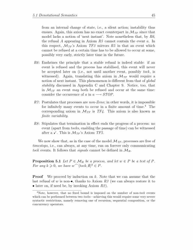
5.1 Denotational Semantics 45
from an internal change of state, i.e., a silent action; instability thusensues. Again, this axiom has no exact counterpart in MTF since thatmodel lacks a notion of ‘next instant’. Note nonetheless that, by R6,the refusal A appearing in Axiom R5 cannot contain the event a. Inthis respect, MTF ’s Axiom TF3 mirrors R5 in that an event whichcannot be refused at a certain time has to be allowed to occur at some,possibly very early, strictly later time in the future.
R6 : Enshrines the principle that a stable refusal is indeed stable: if anevent is refused and the process has stabilised, this event will neverbe accepted later on (i.e., not until another event, possibly tock , iswitnessed). Again, translating this axiom in MTF would require anotion of next instant. This phenomenon is different from that of globalstability discussed in Appendix C and Chapter 9. Notice, too, thatin MTF an event may both be refused and occur at the same time:consider the occurrence of a in a −→ STOP .
R7 : Postulates that processes are non-Zeno; in other words, it is impossiblefor infinitely many events to occur in a finite amount of time.4 Thecorresponding axiom in MTF is TF4. This axiom is also known asfinite variability.
R8 : Stipulates that termination in effect ends the progress of a process: noevent (apart from tocks, enabling the passage of time) can be witnessedafter a X. This is MTF ’s Axiom TF5.
We now show that, as in the case of the model MTF , processes are free oftimestops, i.e., can always, at any time, run on forever only communicatingtock events. It follows that signals cannot be defined in MR.
Proposition 5.1 Let P ∈ MR be a process, and let w ∈ P be a test of P .For any k > 0, we have w_〈tock, ∅〉k ∈ P .
Proof We proceed by induction on k. Note that we can assume that thelast refusal of w is non-•, thanks to Axiom R3 (we can always restore it to• later on, if need be, by invoking Axiom R2 ).
4Note, however, that no fixed bound is imposed on the number of non-tock eventswhich can be performed between two tocks—achieving this would require some very severesyntactic restrictions, namely removing one of recursion, sequential composition, or theconcurrency operators.

5.1 Denotational Semantics 46
The base case k = 0 is, by our assumptions, trivial. For the inductive stepk + 1, let u = w_〈tock , ∅〉k, and suppose that u ∈ P but u_〈tock , ∅〉 /∈ P .Let A be the last refusal of u (the empty set except, possibly, if k = 0). Inany case, we have A 6= •. We can invoke Axiom R4 (with a trivial v = 〈•〉) toconclude that u_〈A∪{tock}〉 ∈ P . This, of course, contradicts the definitionof refusals, which are not allowed to contain the event tock . Consequently,we must have u_〈tock , ∅〉 = w_〈tock , ∅〉k+1 ∈ P , as required. �
In order to define the semantic mapping RJ·K, we need another set ofdefinitions.
If u = 〈A0, a1, A1, . . . , ak, Ak〉 is a test, we let refusals(u) =⋃k
i=0{|Ai|}.Note that refusals(u) is always a set, namely the set of events that are ex-plicitly refused, at one point or another, in u.
We also need the auxiliary function (·) ‖B
(·) : TEST × TEST −→
P(TEST ). Here B ⊆ ΣX, and a, c ∈ Σtock . Let us write Bt = B ∪ {tock}.We proceed inductively on both u and u′ (in defining u ‖
B
u′).
〈A〉 ‖B
〈C〉 = {〈D〉 | D ⊆∗ (B ∩∗ A)∪∗
(B ∩∗ C)∪∗(A∩∗ C)}
〈A, a〉_u ‖B
〈C〉 = 〈A〉 ‖B
〈C〉 if a ∈ Bt
= (〈A〉 ‖B
〈C〉){〈a〉}(u ‖B
〈C〉) if a /∈ Bt
〈A,X〉_u ‖B
〈C〉 = 〈A〉 ‖B
〈C〉 if X ∈ Bt
= (〈A〉 ‖B
〈C〉){〈X〉_u} if X /∈ Bt
〈A〉 ‖B
〈C, c〉_u = 〈C, c〉_u ‖B
〈A〉
〈A〉 ‖B
〈C,X〉_u = 〈C,X〉_u ‖B
〈A〉

5.1 Denotational Semantics 47
〈A, a〉_u1 ‖B
〈C, c〉_u2 = (〈A〉 ‖B
〈C〉){〈a〉}(u1 ‖B
u2) if a = c ∈ Bt
= 〈A〉 ‖B
〈C〉 if a, c ∈ Bt ∧ a 6= c
= (〈A〉 ‖B
〈C〉){〈c〉}
(〈A, a〉_u1 ‖B
u2) if a ∈ Bt ∧ c /∈ Bt
= (〈A〉 ‖B
〈C〉){〈a〉}
(u1 ‖B
〈C, c〉_u2) if a /∈ Bt ∧ c ∈ Bt
= (〈A〉 ‖B
〈C〉){〈a〉}
(u1 ‖B
〈C, c〉_u2)∪
(〈A〉 ‖B
〈C〉){〈c〉}
(〈A, a〉_u1 ‖B
u2) if a, c /∈ Bt
〈A,X〉_u1 ‖B
〈C,X〉_u2 = (〈A〉 ‖B
〈C〉){〈X〉_u1}
〈A,X〉_u1 ‖B
〈C, c〉_u2 = (〈A〉 ‖B
〈C〉) if X ∈ Bt ∧ c ∈ Bt
= (〈A〉 ‖B
〈C〉){〈c〉}
(〈A,X〉_u1 ‖B
u2) if X ∈ Bt ∧ c /∈ Bt
= (〈A〉 ‖B
〈C〉){〈X〉_u1} if X /∈ Bt ∧ c ∈ Bt
= (〈A〉 ‖B
〈C〉){〈X〉_u1}∪
(〈A〉 ‖B
〈C〉){〈c〉}
(〈A,X〉_u1 ‖B
u2) if X /∈ Bt ∧ c /∈ Bt
〈A, a〉_u1 ‖B
〈C,X〉_u2 = 〈C,X〉_u2 ‖B
〈A, a〉_u1.
Likewise, we define the auxiliary function (·) 9 (·) : TEST × TEST −→P(TEST ). Here a, c ∈ Σ. We proceed in a manner similar to the above:
〈A〉 9 〈C〉 = {〈D〉 | D ⊆∗ A∩∗ C}
〈A, a〉_u 9 〈C〉 = (〈A〉 9 〈C〉){〈a〉}(u 9 〈C〉)
〈A,X〉_u 9 〈C〉 = (〈A〉 9 〈C〉){〈X〉_u}
〈A, tock〉_u 9 〈C〉 = 〈A〉 9 〈C〉

5.1 Denotational Semantics 48
〈A〉 9 〈C, c〉_u = 〈C, c〉_u 9 〈A〉
〈A〉 9 〈C,X〉_u = 〈C,X〉_u 9 〈A〉
〈A〉 9 〈C, tock〉_u = 〈C, tock〉_u 9 〈A〉
〈A, a〉_u1 9 〈C, c〉_u2 = (〈A〉 9 〈C〉){〈a〉}
(u1 9 〈C, c〉_u2)∪
(〈A〉 9 〈C〉){〈c〉}
(〈A, a〉_u1 9 u2)
〈A, a〉_u1 9 〈C,X〉_u2 = (〈A〉 9 〈C〉){〈a〉}
(u1 9 〈C,X〉_u2)∪
(〈A〉 9 〈C〉){〈X〉_u2}
〈A, a〉_u1 9 〈C, tock〉_u2 = (〈A〉 9 〈C〉){〈a〉}
(u1 9 〈C, tock〉_u2)
〈A,X〉_u1 9 〈C,X〉_u2 = (〈A〉 9 〈C〉){〈X〉_u1}
〈A,X〉_u1 9 〈C, tock〉_u2 = (〈A〉 9 〈C〉){〈X〉_u1}
〈A, tock〉_u1 9 〈C, tock〉_u2 = (〈A〉 9 〈C〉){tock}(u1 9 u2)
〈A,X〉_u1 9 〈C, c〉_u2 = 〈C, c〉_u2 9 〈A,X〉_u1
〈A, tock〉_u1 9 〈C, c〉_u2 = 〈C, c〉_u2 9 〈A, tock〉_u1
〈A, tock〉_u1 9 〈C,X〉_u2 = 〈C,X〉_u2 9 〈A, tock〉_u1.
We define inductively a hiding operator on tests, of the form (·) \ A :TEST −→ TEST . Here A ⊆ Σ.
〈B〉 \ A = 〈B〉 if A ⊆∗ B
= 〈•〉 if A *∗ B
(〈B, a〉_u) \ A = u \ A if a ∈ A
= (〈B〉 \ A)_〈a〉_(u \ A) if a /∈ A.
Let A ⊆ ΣX. A test u is A-urgent if, whenever 〈B, tock〉 in u, thenA ⊆∗ B. If A = {a} is a singleton, we write a-urgent instead of {a}-urgent.
We define a function RefCl : TEST −→ P(TEST ): for u a test, we letv ∈ RefCl(u) if v ≺ u ∧ trace(v) = trace(u). We extend the definition of RefCl
to sets of tests by setting, for P ⊆ TEST , RefCl(P ) =⋃{RefCl(u) | u ∈ P}.
If f : Σ −→ Σ is a renaming function and u = 〈A0, a1, A1, . . . , ak, Ak〉 ∈TEST , we define f(u) = 〈f(A0), f(a1), f(A1), . . . , f(ak), f(Ak)〉, where f is

5.1 Denotational Semantics 49
extended to ΣXtock
so that f(tock) = tock and f(X) = X, and f(Ai) is either• if Ai = •, or {f(a) | a ∈ Ai} otherwise.
As one would expect, semantic bindings in this model are functions ρ :VAR −→ MR. Again, we write ρ[X := P ] to denote the semantic bindingthat is the same as ρ except that it returns P for X instead of ρ(X). Similarly,λx.ρ[X := x] represents a function which, when fed an element P of MR,returns the semantic binding ρ[X := P ]. Here X ∈ VAR, and x is a bonafide variable (not an element of VAR!) ranging over MR.
For F : MR −→ MR, we define fix(F ) to be the unique fixed point of Fin MR. We stipulate for convenience that, should F not have a fixed point,or should this fixed point not be unique, fix(F ) should denote an arbitrary,but fixed, element of MR.
We now define the function RJ·K inductively over the structure of TimedCSP terms. Since a term P may contain free variables, we also require asemantic binding ρ in order to assign MR processes to the free variables ofP .5 In what follows, u, u1, u2, v, w ∈ TEST , a, ci ∈ ΣX
tock, A ⊆ Σ, B ⊆ ΣX,
and Ci ∈ REF . The rules are as follows:
RJSTOPKρ = {u | trace(u) ≤ 〈tock〉∞}
RJSKIPKρ = {u | trace(u) ≤ 〈tock〉∞ ∧ X /∈ refusals(u)}∪
{u_〈X〉_v | trace(u) ≤ 〈tock〉∞ ∧
X /∈ refusals(u) ∧ trace(v) ≤ 〈tock〉∞}
RJWAIT nKρ = {u | 0 6 k < n ∧ trace(u) = 〈tock〉k}∪
{u_v | trace(u) = 〈tock〉n ∧
trace(v) ≤ 〈tock〉∞ ∧ X /∈ refusals(v)}∪
{u_v_〈X〉_w | trace(u) = 〈tock〉n ∧
trace(v) ≤ 〈tock〉∞ ∧ X /∈ refusals(v) ∧
trace(w) ≤ 〈tock〉∞}
5As was the case for the timed failures model, what we are really defining here is amapping R : TCSP × BIND −→ MR, where BIND stands for the set of all semanticbindings. However, since it again turns out that the denotational values of TCSP programs
are independent of semantic bindings, this point should not overly concern us.

5.1 Denotational Semantics 50
RJP1
n� P2Kρ = {u | 〈tock〉n � trace(u) ∧ u ∈ RJP1Kρ}∪
{u_〈•〉_v | trace(u) = 〈tock〉n ∧
〈tock〉 � trace(v) ∧ u_v ∈ RJP1Kρ}∪
{u_v | trace(u) = 〈tock〉n ∧ u ∈ RJP1Kρ ∧
v ∈ RJP2Kρ}
RJa −→ P Kρ = {u | trace(u) ≤ 〈tock〉∞ ∧ a /∈ refusals(u)}∪
{u_〈a〉_v | trace(u) ≤ 〈tock〉∞ ∧
a /∈ refusals(u) ∧ v ∈ RJP Kρ}
RJa : A −→ P (a)Kρ = {u | trace(u) ≤ 〈tock〉∞ ∧ A ∩ refusals(u) = ∅}∪
{u_〈a〉_v | a ∈ A ∧ trace(u) ≤ 〈tock〉∞ ∧
A ∩ refusals(u) = ∅ ∧ v ∈ RJP (a)Kρ}
RJP1 2 P2Kρ = {u | trace(u) ≤ 〈tock〉∞ ∧ u ∈ RJP1Kρ ∩RJP2Kρ}∪
{u_〈a〉_v | trace(u) ≤ 〈tock〉∞ ∧ a 6= tock ∧
u_〈a〉_v ∈ RJP1Kρ ∪RJP2Kρ ∧
u ∈ RJP1Kρ ∩RJP2Kρ}
RJP1 u P2Kρ = RJP1Kρ ∪RJP2Kρ
RJP1 ‖B
P2Kρ = {u | ∃u1, u2 � u ∈ u1 ‖B
u2 ∧
u1 ∈ RJP1Kρ ∧ u2 ∈ RJP2Kρ}
RJP1 9 P2Kρ = {u | ∃u1, u2 � u ∈ u1 9 u2 ∧
u1 ∈ RJP1Kρ ∧ u2 ∈ RJP2Kρ}
RJP1 ; P2Kρ = RefCl({u \ X | trace(u) � X = 〈〉 ∧
u is X-urgent ∧ u ∈ RJP1Kρ})∪
RefCl({ (u1 \ X)_u2 | trace(u1) � X = 〈〉 ∧
u1 is X-urgent ∧ u1_〈X, •〉 ∈ RJP1Kρ ∧
u2 ∈ RJP2Kρ})
RJP \ AKρ = RefCl({u \ A | u is A-urgent ∧ u ∈ RJP Kρ})
RJf−1(P )Kρ = {u | f(u) ∈ RJP Kρ}
RJf(P )Kρ = {〈C0, f(c1), C1, . . . , f(ck), Ck〉 | k > 0 ∧
〈f−1(C0), c1, f−1(C1), . . . , ck, f
−1(Ck)〉 ∈ RJP Kρ}
RJXKρ = ρ(X)
RJµX � P Kρ = fix(λx.RJP K(ρ[X := x])).
We first need to show that FT J·K is well-defined.
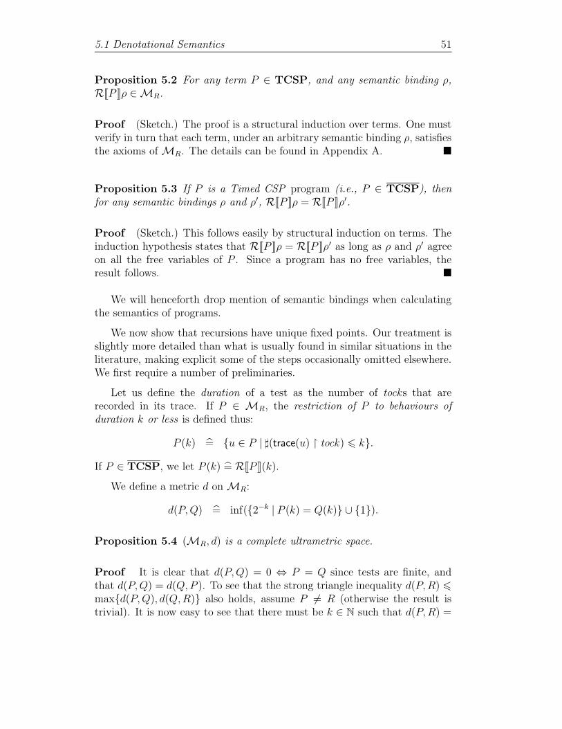
5.1 Denotational Semantics 51
Proposition 5.2 For any term P ∈ TCSP, and any semantic binding ρ,RJP Kρ ∈ MR.
Proof (Sketch.) The proof is a structural induction over terms. One mustverify in turn that each term, under an arbitrary semantic binding ρ, satisfiesthe axioms of MR. The details can be found in Appendix A. �
Proposition 5.3 If P is a Timed CSP program (i.e., P ∈ TCSP), thenfor any semantic bindings ρ and ρ′, RJP Kρ = RJP Kρ′.
Proof (Sketch.) This follows easily by structural induction on terms. Theinduction hypothesis states that RJP Kρ = RJP Kρ′ as long as ρ and ρ′ agreeon all the free variables of P . Since a program has no free variables, theresult follows. �
We will henceforth drop mention of semantic bindings when calculatingthe semantics of programs.
We now show that recursions have unique fixed points. Our treatment isslightly more detailed than what is usually found in similar situations in theliterature, making explicit some of the steps occasionally omitted elsewhere.We first require a number of preliminaries.
Let us define the duration of a test as the number of tocks that arerecorded in its trace. If P ∈ MR, the restriction of P to behaviours ofduration k or less is defined thus:
P (k) = {u ∈ P | ](trace(u) � tock) 6 k}.
If P ∈ TCSP, we let P (k) = RJP K(k).
We define a metric d on MR:
d(P,Q) = inf({2−k | P (k) = Q(k)} ∪ {1}).
Proposition 5.4 (MR, d) is a complete ultrametric space.
Proof It is clear that d(P,Q) = 0 ⇔ P = Q since tests are finite, andthat d(P,Q) = d(Q,P ). To see that the strong triangle inequality d(P,R) 6max{d(P,Q), d(Q,R)} also holds, assume P 6= R (otherwise the result istrivial). It is now easy to see that there must be k ∈ N such that d(P,R) =

5.1 Denotational Semantics 52
2−k. In other words, P (k) = R(k) but P (k + 1) 6= R(k + 1). If Q =P , the result follows. Otherwise, we argue again that P and Q have thesame behaviour up to, but not exceeding, duration k′: P (k′) = Q(k′) butP (k′ + 1) 6= Q(k′ + 1). Now if k′ 6 k, we are done. Otherwise, we must haveP (k+1) = Q(k+1), which of course implies that Q(k+1) 6= R(k+1). Thusd(Q,R) = 2−k, and again the triangle inequality is satisfied.
To establish completeness, let 〈Pi〉i∈N be a Cauchy sequence in MR. Let〈nj〉j∈N be a sequence of positive integers such that, for all j, and for allm > nj, d(Pnj
, Pm) 6 2−j. Let P =⋃
j>0{Pnj(j)}.
We claim that P ∈ MR and that P = limi→∞
Pi. All of the axioms of MR,
with the possible exception of R7, are plain consequences of the definition ofP and the fact that each Pi ∈ MR. For R7, note that whenever u ∈ P is atest of duration k, then u ∈ Pnk
(k). Since Pnksatisfies R7, then so must P .
Lastly, we show that the Pi’s converge to P . Let j > 0 be given. Bydefinition of P we have Pnj
(j) ⊆ P (j), and therefore for all m > nj wehave Pm(j) ⊆ P (j). On the other hand, if u ∈ P (j) is a test of durationk(6 j), we must have u ∈ Pm(k) for some m and hence for all m sufficientlylarge (in fact, it clearly suffices that m > nj). Since Pm(k) ⊆ Pm(j), we getPm(j) = P (j) for all sufficiently large m, or in other words d(Pm, P ) 6 2−j
for all sufficiently large m, as required. �
Note that ultrametric spaces are of course also metric spaces.
It is clear from the definition of the semantic mapping FT J·K above thatevery Timed CSP operator apart from X and µX can be defined as anoperator of the appropriate parity on MR. For example, STOP correspondsto a nullary operator, a −→ (·) corresponds to a unary operator, and (·) 2 (·)corresponds to a binary operator. The definition of these over MR can belifted verbatim from the definition of FT J·K, with an identical proof of well-definedness.
Terms in TCSP may be viewed as ‘formal functions’ in a certain algebra,with variables taken from the set VAR. By the above, each term representsa bona fide function F : MR
k −→ MR, for some k ∈ N. The µX operatoris once again interpreted as computing unique fixed points (yielding an arbi-trary, but fixed, value should no unique fixed point exist). The value of k isthe arity of the formal function. a −→ X, for instance, has arity 1, STOP
has arity 0, and µX � b3
−→ (X ‖ Y ) has arity 1, since the variable X in it isbound. Note that the formal functions X and Y , both of arity 1, technicallyrepresent the same function Id : MR −→ MR, but are formally considered

5.1 Denotational Semantics 53
to be distinct; and indeed, the functions associated with the terms X 9 Yand X 9 X are clearly different. From now on, we will abuse notation andidentify terms with functions, while keeping track of the names of the freevariables.
For any k ∈ N, we construe the space MRk as an ultrametric space by
imposing the ‘sup’ metric on it: if ~P = (P1, P2, . . . , Pk), and similarly for ~Q,
we let d( ~P , ~Q) = sup{d(Pi, Qi) | 1 6 i 6 k}.
Let F : (M1, d1) −→ (M2, d2) be a mapping of metric spaces. We saythat F is non-expanding if, for all x, y ∈ M1, d2(F (x), F (y)) 6 d1(x, y), andthat F is a contraction if there exists δ < 1 such that, for all x, y ∈ M1,d2(F (x), F (y)) 6 δd1(x, y).
If F = F (X, ~Y ) represents a function of arity k + 1, we denote by
F~Y = F~Y (X) the associated function of arity 1 in which ~Y is fixed. (Strictlyspeaking, there is a whole family of such functions, one for each possiblevalue that ~Y could take in MR
k.)
A function F = F (X, ~Y ) is non-expanding in X if F~Y is non-expanding
for each choice of ~Y ∈ MRk, and likewise F is a contraction in X if F~Y is
a contraction for all ~Y . Note that a function is always a contraction in anyvariable which does not occur freely in it.
Lemma 5.5
1. Any contraction is non-expanding.
2. A function is non-expanding (resp. a contraction) if and only if it isnon-expanding (resp. a contraction) in each variable separately.
3. The composition of non-expanding functions is non-expanding.
4. If all the arguments to a non-expanding function represent contractionsin a given variable, then the whole composition is a contraction in thatvariable.
5. Likewise, if all the arguments to a contraction are non-expanding func-tions, then the result is still a contraction.
We omit the straightforward proof. Note that these results hold in arbi-trary metric spaces, provided (for 2.) that we use the sup metric in productspaces.

5.2 Operational Semantics 54
Lemma 5.6 Every term in TCSP is (i.e., corresponds to) a non-expanding
function. Moreover, if P = P (X, ~Y ) is a term which is time-guarded for X,then P is a contraction in X.
Proof (Sketch.) We show that every Timed CSP operator apart fromrecursion is non-expanding by noting that every behaviour of duration k pre-scribed by the operator originates from behaviours of duration no greaterthan k in its arguments. In the case of µX, an examination of the construc-tion of the fixed point as per the Banach fixed point theorem (Theorem A.8)yields the required result. This rests on the fact that time-guardedness fora variable corresponds to contraction in that variable. We demonstrate thisby observing that, if P is time-guarded for X, it follows that behaviours ofX of duration k give rise to behaviours of P of duration at least k + 1; thisentails that P is a contraction in X. Details can be found in Appendix A.
�
Proposition 5.7 Let P = P (X, ~Y ) be a TCSP term which is time-guarded
for X. Then µX � P is the unique function F = F (~Y ) such that F (~Y ) =
P (F (~Y ), ~Y ).
Proof (Sketch.) This follows from the previous lemma and the Banachfixed point theorem. Details are in Appendix A. �
A noteworthy special case arises when P = P (X) has only one free vari-able. Proposition 5.7 then asserts that µX � P ∈ MR is the unique solutionto the equation X = P .
5.2 Operational Semantics
We now present an operational semantics for TCSP programs and establisha congruence theorem relating it to the denotational semantics given in theprevious section. The format is similar to that of Section 3.2, listing a set ofrules of inference from which one can construct the labelled transition system(LTS) of any program.
In contrast with the operational semantics laid out in Chapter 3, here itwould be possible to develop an operational semantics in which all internalcomputational states (or nodes) have representations as TCSP programs.
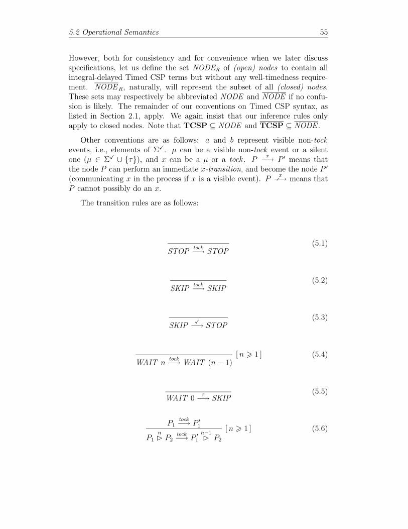
5.2 Operational Semantics 55
However, both for consistency and for convenience when we later discussspecifications, let us define the set NODER of (open) nodes to contain allintegral-delayed Timed CSP terms but without any well-timedness require-ment. NODER, naturally, will represent the subset of all (closed) nodes.These sets may respectively be abbreviated NODE and NODE if no confu-sion is likely. The remainder of our conventions on Timed CSP syntax, aslisted in Section 2.1, apply. We again insist that our inference rules onlyapply to closed nodes. Note that TCSP ⊆ NODE and TCSP ⊆ NODE .
Other conventions are as follows: a and b represent visible non-tockevents, i.e., elements of ΣX. µ can be a visible non-tock event or a silentone (µ ∈ ΣX ∪ {τ}), and x can be a µ or a tock . P
x−→ P ′ means that
the node P can perform an immediate x-transition, and become the node P ′
(communicating x in the process if x is a visible event). Px
X−→ means thatP cannot possibly do an x.
The transition rules are as follows:
STOPtock−→ STOP
(5.1)
SKIPtock−→ SKIP
(5.2)
SKIPX
−→ STOP(5.3)
WAIT ntock−→ WAIT (n − 1)
[ n > 1 ] (5.4)
WAIT 0τ
−→ SKIP(5.5)
P1tock−→ P ′
1
P1
n� P2
tock−→ P ′
1
n−1� P2
[ n > 1 ] (5.6)

5.2 Operational Semantics 56
P1
0� P2
τ−→ P2
(5.7)
P1τ
−→ P ′1
P1
n� P2
τ−→ P ′
1
n� P2
(5.8)
P1a
−→ P ′1
P1
n� P2
a−→ P ′
1
(5.9)
(a −→ P )tock−→ (a −→ P )
(5.10)
(a −→ P )a
−→ P(5.11)
(a : A −→ P (a))tock−→ (a : A −→ P (a))
(5.12)
(a : A −→ P (a))b
−→ P (b)[ b ∈ A ] (5.13)
P1tock−→ P ′
1 P2tock−→ P ′
2
P1 2 P2tock−→ P ′
1 2 P ′2
(5.14)
P1τ
−→ P ′1
P1 2 P2τ
−→ P ′1 2 P2
P2τ
−→ P ′2
P1 2 P2τ
−→ P1 2 P ′2
(5.15)
P1a
−→ P ′1
P1 2 P2a
−→ P ′1
P2a
−→ P ′2
P1 2 P2a
−→ P ′2
(5.16)

5.2 Operational Semantics 57
P1 u P2τ
−→ P1 P1 u P2τ
−→ P2
(5.17)
P1tock−→ P ′
1 P2tock−→ P ′
2
P1 ‖B
P2tock−→ P ′
1 ‖B
P ′2
(5.18)
P1µ
−→ P ′1
P1 ‖B
P2µ
−→ P ′1 ‖
B
P2
[ µ /∈ B, µ 6= X ] (5.19a)
P2µ
−→ P ′2
P1 ‖B
P2µ
−→ P1 ‖B
P ′2
[ µ /∈ B, µ 6= X ] (5.19b)
P1a
−→ P ′1 P2
a−→ P ′
2
P1 ‖B
P2a
−→ P ′1 ‖
B
P ′2
[ a ∈ B ] (5.20)
P1X
−→ P ′1
P1 ‖B
P2X
−→ P ′1
[X /∈ B ]P2
X−→ P ′
2
P1 ‖B
P2X
−→ P ′2
[X /∈ B ] (5.21)
P1tock−→ P ′
1 P2tock−→ P ′
2
P1 9 P2tock−→ P ′
1 9 P ′2
(5.22)
P1µ
−→ P ′1
P1 9 P2µ
−→ P ′1 9 P2
[ µ 6= X ] (5.23a)
P2µ
−→ P ′2
P1 9 P2µ
−→ P1 9 P ′2
[ µ 6= X ] (5.23b)
P1X
−→ P ′1
P1 9 P2X
−→ P ′1
P2X
−→ P ′2
P1 9 P2X
−→ P ′2
(5.24)

5.2 Operational Semantics 58
P1tock−→ P ′
1 P1X
X−→
P1 ; P2tock−→ P ′
1 ; P2
(5.25)
P1X
−→ P ′1
P1 ; P2τ
−→ P2
(5.26)
P1µ
−→ P ′1
P1 ; P2µ
−→ P ′1 ; P2
[ µ 6= X ] (5.27)
Ptock−→ P ′ ∀ a ∈ A � P
aX−→
P \ Atock−→ P ′ \ A
(5.28)
Pa
−→ P ′
P \ Aτ
−→ P ′ \ A[ a ∈ A ] (5.29)
Pµ
−→ P ′
P \ Aµ
−→ P ′ \ A[ µ /∈ A ] (5.30)
Ptock−→ P ′
f−1(P )tock−→ f−1(P ′)
(5.31)
Pµ
−→ P ′
f−1(P )µ
−→ f−1(P ′)[ µ ∈ {τ,X} ] (5.32)
Pf(a)−→ P ′
f−1(P )a
−→ f−1(P ′)(5.33)
Ptock−→ P ′
f(P )tock−→ f(P ′)
(5.34)

5.2 Operational Semantics 59
Pµ
−→ P ′
f(P )µ
−→ f(P ′)[ µ ∈ {τ,X} ] (5.35)
Pa
−→ P ′
f(P )f(a)−→ f(P ′)
(5.36)
µX � Pτ
−→ P [(µX � P )/X].(5.37)
The remark made in Section 3.2 concerning negative premisses (appearingin Rules 5.25 and 5.28) applies here as well.
The effects of these rules follow our intuition: Rule 5.10, for instance,ensures the unhindered passage of time in a prefixed process; Rule 5.14 guar-antees the temporal soundness of external choice; Rules 5.18 and 5.22 forcetime to flow at a uniform rate; and Rules 5.25 and 5.28 implement τ -urgency.Notice, too, the one-to-one correspondence between these rules and theircounterparts in Section 3.2; this will be formally exploited in Proposition 6.2in the next chapter.
The operational semantics enjoys a number of properties, which we listafter the following definitions.
If P and Q are open nodes, we write P ≡ Q to indicate that P and Qare syntactically identical.
If P is a closed node, we define initτR(P ) (initτ (P ) for short) to be the
set of visible non-tock and silent events that P can immediately perform:
initτR(P ) = {µ ∈ ΣX ∪ {τ} | Pµ
−→}. We also write initR(P ) (init(P ) forshort) to represent the set of visible non-tock events that P can immediatelyperform: initR(P ) = initτR(P ) ∩ ΣX.
For P a closed node, we define an execution of P to be a sequence e =P0
x1−→ P1x2−→ . . .
xn−→ Pn (with n > 0), where P0 ≡ P , the Pi’s are nodes,
and each transition Pi
xi+1−→ Pi+1 in e is validly allowed by the operational
inference Rules 5.1–5.37. Here we have each xi ∈ ΣXtock
∪ {τ}. The set ofexecutions of P is written execR(P ), or exec(P ) for short when no confusionis likely. By convention, writing down a transition (or sequence thereof) suchas P
a−→ P ′ is equivalent to stating that P
a−→ P ′ ∈ exec(P ).
5.2 Operational Semantics 60
For P a closed node, the P -rooted graph, or labelled transition system,incorporating all of P ’s possible executions is denoted LTSR(P ), or LTS(P )if no confusion is likely.
If tr = 〈x1, x2, . . . , xn〉 is a τ -trace (i.e., tr ∈ (ΣXtock
∪ {τ})?), we write
Ptr
=⇒ P ′ to mean that there is some execution P0x1−→ P1
x2−→ . . .xn−→ Pn of
P , with P ≡ P0 and P ′ ≡ Pn, which communicates the τ -trace tr . Ptr
=⇒
means that there is some node P ′ such that Ptr
=⇒ P ′, where P〈〉
=⇒ P simplyrepresents the trivial execution P ∈ exec(P ).
The proofs of several of the propositions below are straightforward struc-tural inductions on nodes, carried out in a manner similar to that of [Sch95];in such cases we will therefore omit the details, with the exception of Propo-sition 5.13 (finite variability), the proof of which is quite interesting and in-structive. Alternatively, these propositions can also be seen to follow directlyfrom their counterparts in Section 3.9, thanks to Proposition 6.2, presentedin the next chapter.
The following propositions are universally quantified over P, P ′, P ′′, whichrepresent closed nodes; we are also using n,m, k, k′ to represent natural num-bers, etc. As mentioned above, the reader will notice the correspondencebetween the propositions listed here and those of Section 3.2; it is equallyinteresting to remark on the propositions of Section 3.2 which do not havecounterparts here, such as Proposition 3.5 (time continuity)—this, of course,was to be expected given that the model studied in this chapter is discretein nature.
Proposition 5.8 Time determinacy:
(Ptock−→ P ′ ∧ P
tock−→ P ′′) ⇒ P ′ ≡ P ′′.
Note that a trivial induction extends this result to an arbitrary number oftocks.
Proof (Sketch.) Let us illustrate two cases of the structural induction.
case P1 9 P2: Observe that the only rule allowing P1 9 P2 to communicate
a tock is Rule 5.22, whose conclusion is P1 9 P2tock−→ P ′
1 9 P ′2. The
antecedents of this rule require that P1tock−→ P ′
1 and P2tock−→ P ′
2. Apply-ing the induction hypothesis to P1 and P2 tells us that P ′
1 and P ′2 are
unique, and therefore that so too is P ′1 9 P ′
2, as required.

5.2 Operational Semantics 61
case µX � P : This case follows vacuously since no operational rule allows arecursive term to communicate a tock ; the only behaviour permitted isthe unwinding of the recursion, which results in a τ action.
Note that structural inductions such as the one above must technicallybe carried out over open nodes, together with syntactic bindings. However inmany situations, including the one at hand, the case of recursion is dischargedvacuously under any syntactic binding, which greatly simplifies matters. �
Proposition 5.9 Persistency—the set of possible initial visible events re-mains constant under the occurrence of tocks:
Ptock−→ P ′ ⇒ init(P ) = init(P ′).
Again, this generalises to an arbitrary number of tocks. We omit the proof,but remark that a change in the set of possible initial visible events can onlyarise after the occurrence of a non-tock , visible or hidden, event.
Proposition 5.10 Maximal progress, or τ -urgency:
Pτ
−→ ⇒ PtockX−→.
Proof (Sketch.) This is again a straightforward structural induction. Wecover the case of the hiding operator as an illustration.
First note that any tock -transition of P \ A (with A ⊆ Σ) can only occuras a result of an application of Rule 5.28. Now suppose that P \ A
τ−→. Two
cases arise, depending on whether this τ -transition results from Rule 5.29 orfrom Rule 5.30. The first case violates the second antecedent of Rule 5.28,which therefore disallows P \ A from performing a τ action. In the second
case, we can apply the induction hypothesis (which informs us that PtockX−→)
to conclude that the first antecedent of Rule 5.28 fails to be satisfied. Ineither case, therefore, P \ A is unable to communicate a tock . �
Corollary 5.11
(P〈tock〉n
=⇒ P ′ τ−→ ∧ P
〈tock〉m
=⇒ P ′′ τ−→) ⇒ n = m.

5.2 Operational Semantics 62
Proposition 5.12 A node P can always perform a sequence of tocks up tothe point of the next τ action, or up to any point if no τ action lies ahead:
∀ k > 1 � (@ P ′ � P〈tock〉k
=⇒ P ′) ⇒ ∃ k′ < k, P ′′ � P〈tock〉k
′
=⇒ P ′′ τ−→.
Proposition 5.13 Finite variability—a program P ∈ TCSP cannot per-form unboundedly many actions within a finite number of tocks:
∀ k > 0 � ∃n = n(P, k) � ∀ tr ∈ (ΣXtock
∪ {τ})?�
(Ptr
=⇒ ∧ ](tr � tock) 6 k) ⇒ ]tr 6 n.
We remark that this result holds on account of the fact that programs arewell-timed. Note also that this formulation of finite variability is strongerthan that postulated by Axiom R7, since the latter does not take silent eventsinto account.
Proof (Sketch.) Two proofs of this proposition can be given. The easiestone, by contradiction, is to observe that any failure of finite variability in thecurrent operational semantics would entail a similar failure of finite variability(Proposition 3.9) in the operational semantics for MTF , via Proposition 6.2.This proof is unfortunately not self-contained, since it hinges on an outsideresult (Proposition 3.9, taken from [Sch95]).
The second proof, this one direct, proceeds by structural induction. Thedifficult case is that of recursion, for which the notion of time-bisimulation,similar to that of indexed bisimulation, is introduced and extensively em-ployed. We present the details in Appendix A. �
We now establish a congruence theorem between the operational anddenotational semantics presented in this chapter. Such a theorem providesinstructions to elicit, from the labelled transition system of a program, a setof tests, and then asserts that this set is in fact equal to the denotationalrepresentation of the program in MR.
The techniques required to prove congruence theorems of this kind withinCSP frameworks are well-known and described in, among others, [Ros97] (forstandard, untimed CSP), [Muk93] (for the refusal testing model), and [Sch95](for the timed failures model). Our result relies on similar methods.
A refusal A ∈ REF is refused by a node P if either A is the null refusal•, or P is stable (cannot perform a τ -transition) and has no valid initial

5.3 Refinement and Specification 63
transition labelled with an event from A: P ref A if A = • ∨ (Pτ
X−→ ∧|A| ∩ init(P ) = ∅).
Any execution of a program P gives rise to a set of tests by removingprograms and τ -transitions from the execution, and inserting as refusals,between the remaining transitions, sets of events that cannot be performed.In detail, letting e be an execution of P and u a test, we define inductivelythe relation e test u by induction on e:
P test 〈A〉 ⇔ P ref A
(Pτ
−→)_e′ test u ⇔ e′ test u
(Px
−→)_e′ test 〈A, x〉_u′ ⇔ x 6= τ ∧ P ref A ∧ e′ test u′.
We can now define the function ΦR, which extracts the denotational rep-resentation of a program from its set of executions.
Definition 5.2 For P ∈ NODER, we set
ΦR(P ) = {u | ∃ e ∈ execR(P ) � e test u}.
The chief congruence result now reads:
Theorem 5.14 For any TCSP program P , we have
ΦR(P ) = RJP K.
Proof (Sketch.) The statement must first be rephrased in slightly moregeneral terms, as an assertion about TCSP terms and syntactic bindingsrather than simply programs. In doing so, it proves convenient to temporar-ily abandon the axioms of MR and work in the raw superspace P(TEST )instead. A structural induction is then carried out, establishing the strongerstatement, which then yields the desired result. Details are in Appendix A.
�
5.3 Refinement and Specification
We can define a partial order on P(TEST ) in the same way as we did onP(TF ):
5.3 Refinement and Specification 64
Definition 5.3 For P,Q ⊆ TEST (and in particular for P,Q ∈ MR), welet P vR Q if P ⊇ Q. For P,Q ∈ TCSP, we write P vR Q to meanRJP K vR RJQK, and P =R Q to mean RJP K = RJQK.
We may drop the subscripts and write simply P v Q, P = Q whenever thecontext is clear.
This order is known as test refinement, or the order of nondeterminism.It has the central property:
P v Q ⇔ P u Q = P.
In [Oua97] we showed that this order makes MR into a complete partialorder, or cpo6. Moreover, we showed that every Timed CSP operator, apartfrom X and µX, corresponds to a continuous function7. µX, on the otherhand, can be seen to be a continuous operator from the space of continuousendofunctions on MR to MR.
MR, however, is not a domain because it lacks a least element, as adirect consequence of finite variability—Axiom R7 . Finite variability, ofcourse, follows from the fact that processes are required to be well-timed. Itcan be shown that it is possible to drop this requirement (as we have donefor instance in the operational setting) and still get a consistent denotationalmodel, although in that case it proves useful to include a divergence compo-nent in the representation of processes—a set of tests after the completionof any of which the process may exhibit divergent behaviour, correspondingto an unbounded sequence of internal (silent) transitions.
This model can be shown to be a domain—a cpo with a least element. MR
is then identified with the subset of processes which satisfy finite variabilityand never diverge. The continuity results we have quoted above persist inthe larger model, which entails that any recursion has a least fixed point,as per Tarski’s theorem (see, e.g., [Ros97]). Of course, this least fixed pointagrees with the unique fixed point computed in MR in the case of well-timedprocesses. An adequate congruence theorem between this model and theoperational semantics given in the previous section can be established, whichshows that it is possible to model Zeno processes in a manner which is fullyconsistent with MR. Not only is this an interesting result in its own right, it
6A partial order M is complete if every directed subset (D ⊆ M is directed if for allx, y ∈ D there exists z ∈ D such that x, y v z) of M has a least upper bound in M .
7A continuous function is one that is monotone and preserves least upper bounds ofdirected sets.

5.3 Refinement and Specification 65
also enables us to use refinement as a versatile specification tool, as we shallshortly see.
We first define a second refinement order—known as trace refinement—between sets of tests (and in particular between MR processes):
Definition 5.4 For any P,Q ⊆ TEST, we let P vT Q ⇔ trace(P ) ⊇trace(Q).
(Here the trace operator was naturally extended to apply to sets of tests.)We overload the notation and extend vT to TCSP programs in the obviousway.
Specifications are assertions concerning processes. We write P � S toexpress the fact that process P (or RJP K if P is a program) meets, or satisfies,the specification S.
As in the case of MTF , MR specifications fall naturally into certain cat-egories. We are particularly (though not exclusively) interested in a type ofspecification known as behavioural specifications. A behavioural specificationis one that is universally quantified over the behaviours of processes. In otherwords, S = S(P ) is a behavioural specification if there is a predicate S ′(u)on tests such that, for any P ,
P � S ⇔ ∀ u ∈ P � S ′(u).
In this case we may abuse notation and identify S with S ′. Note that S ′
itself may be identified with a subset of TEST , namely the set of u ∈ TESTsuch that S ′(u).
A behavioural trace specification S = S(P ) is one for which there existsa predicate S ′(tr) on (ΣX
tock)? such that, for any P ,
P � S ⇔ ∀u ∈ P � S ′(trace(u)).
Once again we may identify S with S ′ if no confusion arises as a result.
Behavioural trace specifications are paradigmatic examples of safety prop-erties, requirements of the type: ‘Nothing bad happens’. We will in factnot consider any other sort of safety properties in this work. Other typesof behavioural specifications include liveness properties, requirements that‘something good not be prevented from happening’. Such specifications aretypically primarily concerned with refusal information.

5.4 Verification 66
We remark as before that any specification S = S(P ) which can be ex-pressed, for a fixed process Q, as Q v P , is automatically behavioural.As an example, let us again consider the safety property S(P ): ‘P cannotperform the event a’. Thanks to our earlier discussion, we can validly ex-press this specification as RUN ΣX−{a} vT P , where RUN A = a : A −→RUN A. We can even express the specification as CHAOSΣX−{a} vR P ,
where CHAOSA = (u{a −→ CHAOSA | a ∈ A} u STOP)1� CHAOSA.8
As we shall see in the next section, the advantage of the refinement for-malism is that it enables us to automatically verify the specification by per-forming a refinement check on a model checker such as FDR.
5.4 Verification
This section addresses the question of automatically checking whether a pro-cess meets a given specification. Since this is not the primary focus of thisthesis, the exposition will remain rather brief and far from exhaustive.
Let P be a TCSP program. Even though the set RJP K of P ’s behavioursis always infinite, in many cases P ’s labelled transition system LTSR(P ) isfinite. A specification S on P can thus often be checked by examining P ’sLTS. We demonstrate this by considering behavioural specifications of thetype Q vR P (for a fixed Q ∈ MR).
In [Muk93], it is shown that there is a natural projection from the re-fusal testing model for (untimed) CSP into the standard failures model, andmoreover that the semantic mapping for the failures model factors throughthis projection. A similar result can be shown to hold for our discrete-timerefusal testing model MR provided that the four conditions listed at the endof Chapter 4—unhindered passage of time, temporal soundness of externalchoice, uniform rate of passage of time, and maximal progress—are somehowadequately incorporated to the failures model. As discussed in Chapter 4,this cannot be done in a purely denotational setting, but can still be achievedoperationally, via a suitable syntactic translation (Ψ), together with the pos-
8Note that our use of the general internal choice operator u, in the definition of
CHAOSA, is simply shorthand for repeated use of the usual internal choice operatoru, since A ⊆ ΣX is finite. We also remark that this definition of CHAOSA, meant tocapture the vR-least process with alphabet A, is slightly more complicated than the usualdefinition seen in standard models of (untimed) CSP, owing to the fact that refusal testinginformation is more discriminating than mere failure information.

5.4 Verification 67
tulation of τ -urgency—the prioritising of silent events over tocks.
Let us therefore consider a specification S on MR processes which is onlyconcerned with failures, i.e., traces together with a final refusal. For anyP ∈ TCSP, to verify that P � S in MR (i.e., that RJP K � S), it is sufficientto show that Ψ(P ) � S in the prioritised failures model, by which we mean themodel in which failures are derived from the prioritised operational semantics.Since this last check can be performed on the model checker FDR, we arealready able to mechanically verify a large class of behavioural specifications.9
(In general this may also involve a suitable translation of the specificationS).
An important subclass of such specifications are safety properties, sincethese are exclusively concerned with traces (and can therefore obviously beexpressed in terms of failures). Thus to verify for example that RJP K nevercommunicates the event a (i.e., that RUN ΣX−{a} vT P ), it is sufficient tocheck that Ψ(RUN ΣX−{a}) vT Ψ(P ) using FDR. Note that the second re-finement must hold if RJP K meets the specification, although the FDR checkwill succeed only if P has a finite (in fact manageable) LTS. We provide aconcrete example of this technique in Section 6.7.
In general, however, we cannot always depend on this sort of analysis,since there are TCSP programs which have distinct interpretations in MR
but have identical sets of failures. In the rare cases where this is likely tocause a problem (namely, in those cases in which the specification on testsunder consideration cannot be expressed purely in terms of failures), one mustdirectly perform an analysis of the LTS of the program to determine whetherthe specification holds or not. We provide an algorithm which achieves thistask in Appendix B, drawing on the notion of power-simulation which lies atthe heart of FDR checks.
9A ‘priority’ operator has been included in beta versions of FDR, but has not, to ourknowledge, been officially released. The incorporation of priority in future versions ofFDR2 is understood to be currently under consideration by Formal Systems Europe Ltd.

Chapter 6
Timed Analysis (I)
We now address the task of extracting information about the continuous-timebehaviour FT JP K of a TCSP program P from its discrete-time representationRJP K.
In Section 6.1 we introduce the notion of the timed denotational expansionof an MR process. This is an entirely straightforward attempt to elicit, ormore precisely to approximate, the continuous-time behaviour of a processfrom its set of tests. We then continue with a section examining a numberof examples highlighting the types of inaccuracies that timed denotationalexpansions exhibit with respect to exact process behaviour.
In Section 6.3, we focus our analysis on timed traces, and develop tools en-abling us to quantitatively assess how closely timed denotational expansionsmatch exact process behaviour. We obtain soundness and quasi-completenesstheorems which essentially show that timed denotational expansions are con-servative approximations of exact behaviour, and moreover that these ap-proximations get better and better as ‘time granularity’ (the number of tockspostulated to occur within one time unit) gets finer and finer.
Section 6.4 then seeks to exploit these observations and results towardsautomated verification, concentrating, once again, on timed traces. Severalavenues are explored, with the most important and mature approach buildingupon a result of Henzinger, Manna, and Pnueli’s. A number of examples arepresented, many of which illustrating the limitations of the various techniquesunder consideration.
Section 6.5 studies the applicability of our techniques and results to full—i.e., timed failures, or safety and liveness—automated verification. This sec-
6.1 Timed Denotational Expansion 69
tion in some sense represents the culmination of our work. We extend thepreviously cited result of Henzinger et al. from timed traces to timed failures,and use it as a foundation to produce exact verification theorems (as well asa corresponding model checking algorithm, described in Appendix B).
Section 6.6 answers many questions regarding the scope and limitations ofthe techniques thus described, particularly in the context of refinement-basedspecifications.
Finally, Section 6.7 offers a small verification case study illustrating theresults and algorithm derived in Sections 6.4 and 6.5.
6.1 Timed Denotational Expansion
If P is a TCSP program, we would like to convert the refusal testing in-formation contained in RJP K into useful information concerning the timedfailures of FT JP K. The general intuition behind our approach is in essencecaptured by the following example: suppose that in a particular test of RJP K,the event a occurs after three tocks, followed by a b, and then a further tock .We would conclude that a and b occurred at times ta and tb, respectively,such that 3 6 ta 6 tb < 4.1 Ideally we would then expect there to be timedfailures in FT JP K accounting for these behaviours, and vice-versa.
To this end, we define a function Expk : MR −→ P(TF ) (where Exp
stands for ‘expansion’, and the integral subscript k indicates how many tocksare meant to be signalled per time unit), to transform MR processes intosets of compatible timed failures.
In detail, the construction goes as follows. Let P ∈ MR and let u =〈A0, a1, A1, a2, . . . , an, An〉 be a test of P . We first define preExpk(u) to bethe set of timed failures (s,ℵ) ∈ TF satisfying the following:
1For technical reasons, we require the third inequality to be strict, but otherwise therecan be no guarantee that events, such as a and b or even tock , did not in fact happen‘simultaneously’.

6.2 Timing Inaccuracies 70
∃(ti ∈ R+)06i6n+1�
0 = t0 6 t1 6 . . . 6 tn < tn+1 = (1 + ](〈a1, a2, . . . , ai〉 � tock))/k ∧
s = 〈(t1, a1), (t2, a2), . . . , (tn, an)〉 \ tock ∧
(∀(1 6 i 6 n)�
ai = tock ⇒ (ti = ](〈a1, a2, . . . , ai〉 � tock)/k ∧ ti−1 6= ti)) ∧
ℵ ⊆n⋃
i=0
{[ti, ti+1) × |Ai|}.
We can now give
Definition 6.1 For any P ∈ MR and k > 1, we define the timed denota-tional expansion Expk(P ) of P to be
Expk(P ) =⋃
{preExpk(u) | u ∈ P}.
(We will usually omit the subscript k when it is equal to 1.)
Note how the basic idea laid out earlier has been extended to refusal setsin the definition of Expk. A point worthy of mention is that the refusal • istreated as if it were the empty refusal set; we will return to this later on.
We also point out that in general, for P ∈ MR, it is not the case thatExpk(P ) is an MTF process, as we shall soon see.
6.2 Timing Inaccuracies
One would ideally like to have the equality FT JP K = Exp(RJP K) for allP ∈ TCSP. Unfortunately this cannot be, for a variety of reasons, as wenow demonstrate. In the analysis below we shall freely switch back and forthbetween denotational and operational interpretations of process execution.
Consider the program P1, defined as follows:
P1 = (a 2 WAIT 1) ; STOP .
The behaviour of P1 in the timed failures model essentially consists in offeringa for one time unit, at which point, if a has not occurred, the subprocessWAIT 1 offers a X. Sequential composition then forces this X to occur,silently, on the spot, unless a occurs instead at that very instant. This

6.2 Timing Inaccuracies 71
latter choice is nondeterministic (and in theory also subject to environmentalcooperation). What is certain is that a cannot occur at any time t > 1.2
The tests of RJP1K exhibit some subtle but important differences: untilthe first tock is recorded, a does not appear in refusals, i.e., a is continuouslyon offer, as expected. However, this situation persists after the occurrence oftock , right up to the time when, operationally, a silentX is performed (by thesubprocess WAIT 1). Refusals in the interim (i.e., between the first tock andthe silent X) are null (•), and a is certainly not prevented from occurring.Our semantics only prescribes that the hidden X occur before the next tock ,which implies that in certain cases P1 will still be able to communicate aat times which are arbitrarily close to that of the second tock occurrence.Accordingly, the timed denotational expansion of RJP1K is unable to ruleout a purported occurrence of a before two full time units have elapsed.In some sense, the nondeterministic uncertainty witnessed throughout thehalf-open time interval of one time unit between the first and second tockscorresponds precisely to the point nondeterminism observed at the instantt = 1 in the timed failures model.
This example also shows that Exp(RJP1K) cannot possibly be an MTF
process; for example, the failure (〈(1.5, a)〉, [0, 1)×(ΣX−{a})) ∈ Exp(RJP1K)is ≺-maximal over the interval [0, 1.5); however, the failure (〈(1, b)〉, [0, 1) ×(ΣX −{a})) does not appear in Exp(RJP1K), violating Axiom TF3. Inciden-tally, note that, for any P ∈ MR, Axiom TF3 is the only one that Expk(P )will possibly fail to satisfy.
The following program exemplifies a slightly different kind of timing un-faithfulness:
P2 = a1
−→ b.
The timed failures of FT JP2K clearly indicate that the time difference betweenthe occurrences of a and b must be greater than or equal to one time unit.In contrast, the tests of RJP2K require that there should be at least onetock between the two events. An application of Exp therefore yields (amongmany others) the timed trace 〈(0.99, a), (1, b)〉, in which the time differencebetween a and b is almost nil! (This difference can in fact be ‘made’ as smallas desired, but never zero as the definition of denotational expansion requiresa to ‘occur’ strictly before the following tock .)
A slightly more dramatic demonstration of the effect of the timing inac-
2P1 in effect implements the timeout process a1
� STOP , but the lengthier expressionwe have chosen for it better illustrates the situation at hand.
6.2 Timing Inaccuracies 72
curacies described above is achieved with the program P3 below:
P3 = (a1
−→ (a0� STOP)) 9 (b
1−→ (b
0� STOP)).
FT JP3K consists of two interleaved processes, each of which can, at anytime, communicate an event, and then communicate it again exactly one timeunit later, or not at all. If we suppose that two a’s and two b’s are witnessedin a given timed failure of FT JP3K, with the first a occurring strictly beforethe first b, then the last event to be communicated will have to be a b.
However, it is easy to see that Exp(RJP3K) contains timed failures whosetimed traces are, for example, 〈(0, a), (0.9, b), (1, b), (1.9, a)〉. Here the seconda ought to have occurred 0.9 time units before the second b, rather than 0.9time units after it! We do note, however, that FT JP3K does contain timedfailures whose untimed traces are 〈a, b, b, a〉; but for this to happen one musthave the initial a and b occurring simultaneously.
One might think that the rather disconcerting state of affairs exposed inthe previous few paragraphs should spell doom for any sustained or valuableuse of MR for accurate analysis of process behaviour in MTF . But it turnsout that the discrepancies noted are themselves worst-case scenarios, and ingeneral the ‘timing fuzziness’ that our discrete analysis necessarily entailsdoes not accumulate and remains satisfactorily bounded. This statement ismade precise in Theorem 6.6 below.
The examples above have exclusively focused on (timed) traces. We nowshow that refusals bring their own unruly twist to the picture. Here problemsarise because MR fails to offer a satisfactory treatment of instability—thetransient state a process finds itself in while hidden events are on offer. Thisis remedied with the model MUR, presented in the next chapter.
The presence of instability is dealt with in MR by sweeping all refusalinformation under the rug, only allowing • as refusals. As far as the definitionof Exp went, this left us with a choice of two evils: either conservatively treat •as if it were the maximum refusal set, ΣX, or (as we did) ignore • altogetherand treat it as the empty refusal set. The first alternative would clearlyhave made any refusal information in the timed denotational expansion ofa process useless, since •, as per Axiom R1 , is always an allowable refusal.Unfortunately, the path we have chosen is only slightly better, as we mustnow cope with the eventuality of under-refusing events.
As an example, let us once more consider P2 = a1
−→ b. Suppose that ana is recorded at time 0.7 in a particular timed failure of FT JP2K. Then b can

6.3 Timed Trace Analysis 73
be validly refused over the interval [0, 1.7), as some other timed failure willbear out. In the timed denotational expansion of RJP2K, however, b will atbest only be refused over the interval [0, 1) (again assuming a was decreedto have happened at time 0.7). Afterwards, a silent X is on offer, leaving a• refusal until such time as it occurs, at which point any event but b will bestably refused.
6.3 Timed Trace Analysis
We now present some general results about the correspondence between MR
and MTF , mostly concerning (timed) traces.
Proposition 6.1 Let P ∈ TCSP, and let e ∈ execTF (P ) be an integralexecution. There exists an integral execution e′ ∈ execTF (P ) all of whoseevolutions have unit duration, and such that, for any timed failure (s,ℵ),e′ fail (s,ℵ) if and only if e fail (s,ℵ).
Although e′ is technically not necessarily unique, we will pretend that it is(choosing a particular execution if necessary) and call it the normalisationof e. Any integral execution only comprising unit duration evolutions, suchas e′, is termed a normal execution.
Proof One first shows by structural induction on Q that, whenever Q0 Q′,
then Q′ ≡ Q. It also follows from Proposition 3.5 that, whenever Qn Q′ (for
n > 1), there is a unique sequence 〈Qi〉ni=0 such that Q0 ≡ Q, Qn ≡ Q′, and
Q01 Q1
1 . . .
1 Qn. Moreover, for all 0 6 i 6 n, initTF (Qi) = initTF (Q).
Given e ∈ execTF (P ) as above, one then replaces every Q0 Q′ in e by Q
and every Qn Q′ in e by Q0
1 Q1
1 . . .
1 Qn. The resulting execution is
clearly the required e′. �
Proposition 6.2 For any P ∈ TCSP, the set of normal executions of P(in the operational semantics associated with MTF ) is in natural one-to-onecorrespondence with the set execR(P ) of executions of P (in the operationalsemantics associated with MR).
More precisely, this bijection takes a normal execution e = P0z17−→ P1
z27−→. . .
zn7−→ Pn ∈ execTF (P ) to the execution e′ = P0x1−→ P1
x2−→ . . .xn−→ Pn ∈

6.3 Timed Trace Analysis 74
execR(P ), where for all 1 6 i 6 n, xi = tock whenzi7−→ =
1 , and xi = µ
whenzi7−→ =
µ−→.
In particular, initτTF
(P ) = initτR(P ).
Proof (Sketch.) This is a straightforward inspection which rests on theperfect bijective correspondence between the operational inference Rules 3.1–3.37 and 5.1–5.37. A formal proof proceeds by structural induction on P .
�
We next define an integral multiplication operation on terms: for P ∈TCSP and k > 1, kP ∈ TCSP is identical to P except that every delay nin P has been replaced by a delay of kn (in all subprocesses WAIT n and
P1
n� P2) in kP . This operation can be given a straightforward inductive
definition, which we omit. Note that integral multiplication takes programsto programs.
We can also define an integral multiplication operation on timed failures.If (s,ℵ) = (〈(ti, ai)〉
ni=1,
⋃m
i=1{[bi, ei)×Ai}) ∈ TF and k > 1, we let k(s,ℵ) =(〈(kti, ai)〉
ni=1,
⋃m
i=1{[kbi, kei)×Ai}) ∈ TF . This definition extends to sets oftimed failures in the obvious way.
Lemma 6.3 For any P ∈ TCSP and k > 1, FT JkP K = kFT JP K.
Proof (Sketch.) One first extends integral multiplication to executions, asfollows. If e = P0
z17−→ P1z27−→ . . .
zn7−→ Pn ∈ execTF (P ), for some arbitrary
program P , we let ke = kP0kz17−→ kP1
kz27−→ . . .kzn7−→ kPn, where each transition
kPi
kzi+17−→ kPi+1 in ke is kPi
µi+1−→ kPi+1 if Pi
zi+17−→ Pi+1 = Pi
µi+1−→ Pi+1, and is
kPi
kti+1 kPi+1 if Pi
zi+17−→ Pi+1 = Pi
ti+1 Pi+1. This operation naturally extends
to sets of executions.
One then shows by structural induction that, for any term P , and anysyntactic binding η with the property that execTF (kη(X)) = kexecTF (η(X))for all X ∈ VAR, the equality execTF (k(Pη)) = kexecTF (Pη) holds. Allinductive cases are straightforward apart from recursion, which is handledusing the indexed bisimulation techniques which figured prominently in theproofs of the digitisation lemma (Lemma 3.11) and Proposition 5.13 (wheretime-bisimulations, rather than indexed bisimulations, were used for the lat-ter).
One then concludes that, for any Q ∈ TCSP, initTF (Q) = initTF (kQ).

6.3 Timed Trace Analysis 75
The result then follows immediately from Theorem 3.10. �
We also have the following result:
Lemma 6.4 For any P ∈ MR and k > 1, Exp(P ) = kExpk(P ).
Proof (Sketch.) Follows immediately from the definitions. �
We can now give:
Theorem 6.5 For any P ∈ TCSP and k > 1,
Expk(RJkP K) vTT FT JP K.
Proof We first observe that, due to Lemmas 6.3 and 6.4, it suffices to provethe result for k = 1.
Fix P ∈ TCSP, and let s ∈ TTraces(FT JP K). Pick an execution e ∈execTF (P ) such that e fail (s,ℵ) for some refusal ℵ, as per Theorem 3.10.Let e′ = [e]1 ∈ execTF (P ) be the lower digitisation of e as per the digi-tisation lemma (Lemma 3.11), and let e′′ be the normalisation of e′, asper Proposition 6.1. By Proposition 6.2, there is a canonical executiono ∈ execR(P ) matching each of e′′’s unit-duration evolutions with tock -transitions, and identical to e′′ in all other respects. Let u ∈ RJP K be suchthat o test u, as per Theorem 5.14. It is easy to verify, given u’s constructionand the definition of preExp, that s ∈ TTraces(preExp(u)), and therefore thats ∈ TTraces(Exp(RJP K)), completing the proof. �
This theorem can be interpreted as a (timed trace) soundness result:if a (presumably undesirable) behaviour is ruled out by the denotationalexpansion of RJP K, then it is certainly not a possible behaviour of FT JP K.(Timed trace) completeness, on the other hand, would be the assertion thatthe reverse refinement holds, i.e., that the only timed traces absent fromthe denotational expansion of RJP K are precisely those which FT JP K cannotperform. But as we have seen in the previous section, this is something wehave to forgo. Nonetheless, we can get a good approximation to (timed trace)completeness, which we present below.
We first need to define a metric td on the space TT of timed traces. Lets = 〈(t1, a1), (t2, a2), . . . , (tn, an)〉 and s′ = 〈(t′1, a1), (t
′2, a2), . . . , (t
′n, an)〉 be
timed traces. We define the timed distance td(s, s′) between them as follows:

6.3 Timed Trace Analysis 76
td(s, s′) = max{(|t′i − ti|) | 1 6 i 6 n}. In all other situations (namely, whenthe untimed versions of s and s′ do not agree), we set td(s, s′) = ∞. td
clearly makes TT into a (complete) metric space.
Theorem 6.6 For any P ∈ TCSP, k > 1, and s ∈ TTraces(Expk(RJkP K)),there exists s′ ∈ TTraces(FT JP K) such that td(s′, s) < 1/k. In fact, s′ can bechosen so that each of its events is recorded earlier than or at the same timeas its vis-a-vis in s.
Proof Here again it follows easily from Lemmas 6.4 and 6.3 that it sufficesto prove the result in the case k = 1.
So let s ∈ TTraces(Exp(RJP K)), and let u be a test of RJP K yielding(s,ℵ) (for some refusal ℵ) under preExp. Theorem 5.14 assures us there is anexecution e ∈ execR(P ) such that e test u, and Proposition 6.2 then informsus that there is an execution e′ ∈ execTF (P ) identical to e but for havingunit-duration evolutions wherever e had tock -transitions. By Theorem 3.10,there is (s′,ℵ′) ∈ FT JP K such that e fail (s′,ℵ′).
Now, by definition, preExp decrees that the time of occurrence of anyevent in a given test must lie in a unit interval consistent with the number oftocks witnessed prior to the event. Clearly, then, the timing of correspond-ing events in preExp(u) and s′ cannot differ by more than one time unit. Weobserve that the inequality is strict since events in preExp(u) must by defi-nition ‘happen’ strictly before the time postulated for the occurrence of thefollowing tock . �
Note that in the case k = 1, each event in s′, as constructed in theproof, happens at the greatest integral time less than or equal to the time ofoccurrence of its vis-a-vis in s; in other words, s′ is the lower digitisation ofs.
Theorem 6.6 is a (timed trace) quasi-completeness result, as it gives ussharp bounds regarding the extent to which timed denotational expansionscan stray from the MTF -computed timed traces of a given TCSP program P .Together with Theorem 6.5, it also shows that, as k increases, Expk(RJkP K)‘converges’ towards FT JP K (at least as far as timed traces are concerned),enabling one’s analysis of FT JP K to become arbitrarily ‘precise’, albeit po-tentially at an expense in computational complexity.
We point out, perhaps surprisingly, that k 6 k′ does not necessarilyentail that Expk(RJkP K) vTT Expk′(RJk′P K) for an arbitrary program P .
6.4 Applications to Verification 77
For example, let P = a −→ (b1� STOP), and compare RJ2P K and RJ3P K
(i.e., k = 2 and k′ = 3). If the original time units are minutes, then twoconsecutive tocks by the first process are meant to delineate a 30s interval,whereas two consecutive tocks by the second process signify that 20s haveelapsed between them. On the trace 〈(25s, a)〉, therefore, E2 = Exp2(RJ2P K)will ‘simulate’ a tock , after a, ahead of E3 = Exp3(RJ3P K). Because ofthis, the latest possible occurrence of b in E2 will arrive sooner than in E3.And indeed, a simple inspection shows that the traces 〈(25s, a), (t, b)〉, with90s 6 t < 100s, are all possible for E3, but not for E2. Hence it is not thecase that E2 vTT E3.
Of course, under certain conditions the expected relationship will hold:
Proposition 6.7 Let P ∈ TCSP, and let 1 6 k 6 k′ be such that k dividesk′. Then Expk(RJkP K) vTT Expk′(RJk′P K).
Proof (Sketch.) It clearly suffices to prove the result in the case k = 1,thanks to Lemma 6.4. Let s ∈ TTraces(Expk′(RJk′P K)). We must show thats ∈ TTraces(Exp(RJP K)). Let u ∈ RJk′P K with s ∈ TTraces(preExpk′(u)). ByTheorem 5.14, there is e ∈ execR(k′P ) such that e test u. Proposition 6.2then provides a corresponding normal execution e′ ∈ execTF (k′P ). As inthe proof of Lemma 6.3, we then therefore have that e′/k′ ∈ execTF (P ). Leto ∈ execTF (P ) be the lower digitisation of e′/k′, as per the digitisation lemma,and let o′ ∈ execTF (P ) be the normalisation of o, as per Proposition 6.1.We can then invoke Proposition 6.2 again to obtain o′′ ∈ execR(P ), whichthen yields v ∈ RJP K, with o′′ test v, by Theorem 5.14. It is then notdifficult to trace through this sequence of transformations and verify thatone has s ∈ TTraces(preExp(v)), and therefore that s ∈ TTraces(Exp(RJP K)),as required. �
It is interesting to note how the above proposition, which is stated entirelyin terms of the discrete-time refusal testing model MR, is established usingresults, such as the digitisation lemma, which are themselves stated purelyin terms of the timed failures model MTF .
6.4 Applications to Verification
We show how the results of the previous section can be exploited to reduceproof obligations in MTF to proof obligations in MR.
6.4 Applications to Verification 78
The most natural instance concerns behavioural specifications. Specifi-cally, if S is a behavioural timed trace specification on MTF processes, Theo-rem 6.5 guarantees that, for any P ∈ TCSP and any k > 1, if Expk(RJkP K) �S, then FT JP K � S as well. The definition of Expk, on the other hand, makesit simple to manufacture a conservative specification C(S), derived from S,such that if RJkP K � C(S), then Expk(RJkP K) � S.
As an example, let us consider the following timed trace specificationS1: ‘Whenever the event b is observed, it must have been preceded at most10 time units earlier by the event a’. This is a behavioural timed tracespecification because it is a predicate required to hold for all the timed tracesof a process.
A TCSP program P will satisfy S1 if RJP K satisfies the test specificationC(S1) that reads: ‘Whenever the event b is observed, it must have beenpreceded by the event a, with at most 9 tocks occurring between them.’ Notehow the time constraint was converted into a requirement on the number oftocks; it is in fact not hard to see intuitively that there is a systematic way toperform such conservative conversions (although making this precise wouldrequire us to set up a formal specification formalism). The drawback, on theother hand, is that there may be some programs P such that FT JP K � S1
but RJP K 2 C(S1).
In the case at hand, for example, a sharper analysis reveals that it is suffi-cient to consider the weaker test specification ZR(S1) that reads: ‘Wheneverthe event b is observed, it must have been preceded by the event a, with atmost 10 tocks occurring between them.’ Indeed, suppose that FT JP K 2 S1
for some program P . Then there is s ∈ TTraces(FT JP K) with 〈(tb, b)〉 in s,and such that whenever 〈(ta, a)〉 in s with ta 6 tb, tb−ta > 10. Let us assumethat there is at least one such instance 〈(ta, a)〉 in s (in which case we pickthe one with largest ta value), otherwise we trivially have RJP K 2 ZR(S1).If tb denotes the fractional part of tb, we can apply the digitisation lemmato (any execution yielding) the timed trace s, with pivot tb, to obtain (anintegral execution yielding) the timed trace [s]tb ∈ TTraces(FT JP K). It isthen clear that the corresponding a and b events in [s]tb occur respectivelyat times btac and dtbe, i.e., at least 11 time units apart. We can then invokeProposition 6.2 to obtain a test u ∈ execR(P ) with at least 11 tocks occurringbetween these very a and b events. In other words, RJP K 2 ZR(S1).
Since, on the other hand, it is clear (again thanks to Proposition 6.2)that for all P ∈ TCSP, FT JP K � S1 implies that RJP K � ZR(S1), we findourselves in the highly desirable situation of having S1-satisfiability equivalentto ZR(S1)-satisfiability.

6.4 Applications to Verification 79
This state of affairs is a particular instance of Theorem 6.10, which wegive below after introducing the necessary terminology.
For T a set of timed traces, let Z(T ) denote the subset of integral timedtraces of T , in other words those timed traces in T all of whose events occurat integral times. For 0 6 ε 6 1, the operator [·]ε, defined in Section 3.3,naturally extends to timed traces (as was implicit in our use of the notation[s]tb above), by pointwise application to the time component of each of thetrace’s elements. We can therefore extend [·]ε further by applying it to setsof timed traces. We then say that the set T is closed under digitisation if,for any 0 6 ε 6 1, [T ]ε ⊆ T . On the other hand, we say that T is closedunder inverse digitisation if, whenever a timed trace s is such that [s]ε ∈ Tfor all 0 6 ε 6 1, then s ∈ T .
The following result is due to Henzinger, Manna, and Pnueli [HMP92]:
Theorem 6.8 If P ⊆ TT is closed under digitisation and S ⊆ TT is closedunder inverse digitisation, then
Z(P ) ⊆ Z(S) ⇔ P ⊆ S.
The next result is a direct consequence of the digitisation lemma:
Theorem 6.9 For any program P ∈ TCSP, TTraces(FT JP K) is closed un-der digitisation.
For any set S ⊆ TT of timed traces, it is easy to see that one can alwaysfind a set of tests ZR(S) ⊆ TEST having the property
Z(S) = Z(TTraces(Exp(ZR(S)))).
(There will always be several choices for ZR(S); let us pick one for eachS ⊆ TT , and thus think of ZR as a function from P(TT ) to P(TEST ).)
Recall that any behavioural timed trace specification can be identifiedwith a set of timed traces: for S such a specification and P a TCSP program,P � S if and only if TTraces(FT JP K) ⊆ S. Given a timed trace specificationS, let us therefore also write ZR(S) to denote the corresponding behaviouraltest specification. We now give our main (timed trace) result:
Theorem 6.10 Let S = S(P ) be a behavioural timed trace specificationclosed under inverse digitisation. Then, for any program P ∈ TCSP,
RJP K � ZR(S) ⇔ FT JP K � S.

6.4 Applications to Verification 80
Proof (Sketch.) Let S be as above. By Theorem 6.8, we have FT JP K �S ⇔ Z(TTraces(FT JP K)) � Z(S). Suppose that RJP K � ZR(S), and lets ∈ Z(TTraces(FT JP K)) be an integral trace of P . We aim to show thats ∈ Z(S). It is easy to show (by structural induction on P ) that there is someintegral execution e ∈ execTF (P ) such that e fail (s, ∅). We can then invokePropositions 6.1 and 6.2 to obtain a corresponding execution o ∈ execR(P )such that o test u, where u ∈ RJP K is a test of P with the property thats ∈ TTraces(preExp(u)). Since RJP K � ZR(S), we have u ∈ ZR(S), andtherefore s ∈ Z(S) by definition of ZR(S), remembering that s is an integraltimed trace. This establishes the left-to-right implication.
The procedure which yielded u from s can equally be carried out in thereverse direction—we leave the details to the reader. This takes care of theright-to-left implication and completes the proof. �
Note that the behavioural timed trace specification S1 defined earlier isclosed under inverse digitisation; an application of Theorem 6.10 thereforeimmediately yields our earlier conclusion that S1-satisfiability is equivalentto ZR(S1)-satisfiability.
Theorem 6.10 yields the following central corollary:
Corollary 6.11 Let Q ∈ TCSP be a program whose set of timed tracesTTraces(FT JQK) is closed under inverse digitisation. Then, for any programP ∈ TCSP,
RJQK vT RJP K ⇔ FT JQK vTT FT JP K.
Proof (Sketch.) This result rests on the fact that RJQK satisfies thecrucial property Z(TTraces(FT JQK)) = Z(TTraces(Exp(RJQK))), which canbe shown using the line of reasoning offered in the proof of Theorem 6.10.The desired conclusion then follows from Theorem 6.10. �
An interesting fact is that closure under inverse digitisation characterisesthose (downward-closed) behavioural timed trace specifications3 that obeythe conclusion of Theorem 6.10, as the following proposition indicates:
Proposition 6.12 Let S = S(P ) be a downward-closed behavioural timedtrace specification which is not closed under inverse digitisation. Then thereis a program P ∈ TCSP such that RJP K � ZR(S) but FT JP K 2 S.
3It makes little sense for behavioural specifications not to be downward-closed, sinceprocesses themselves are always downward-closed.

6.4 Applications to Verification 81
Proof (Sketch.) Let the specification S be as above. There must then bea trace tr = 〈(t1, a1), (t2, a2), . . . , (tn, an)〉 /∈ S such that, for all 0 6 ε 6 1,[tr ]ε ∈ S. We now construct a program P with the following property: anydigitisation of a trace of FT JP K is equal to some digitisation of a prefix of tr ,and moreover FT JP K contains the trace tr .
The idea is fairly simple: we build P in stages, by specifying increasinglystronger restrictions on the allowable times of occurrence of the successiveevents of tr . For any given index 1 6 j 6 n, the allowable times of occur-rence of aj depend on the occurrence times of all events preceding it. Theserestrictions are captured by processes Bj
i , each of which subordinates theallowable times of occurrence of aj to the time of occurrence of ai. (We al-low i to be 0 to also subordinate the occurence of aj to an imaginary eventa0 occurring at time 0.) Those time bounds are then combined by simplyputting the Bj
i ’s in parallel.
To illustrate the idea, consider the allowable times of the first event, a1. Ifa1 has occurred at some integral time (i.e., if t1 ∈ N), then the only allowabletime for a1 is t1. Otherwise, a1 should be free to occur at any time t′1 suchthat bt1c 6 t′1 6 dt1e: any digitisation of t′1 is a digitisation of t1 (althoughnot necessarily involving the same pivot ε). This restriction is captured bythe process B1
0 .
Consider now the allowable times of occurrence of the second event, a2.Like a1, it must be constrained by some B2
0 specifying its ‘absolute’ allowabletimes of occurrence. Moreover, it must also be constrained with respect tot′1 (a1’s time of occurrence). For instance, if the difference between t2 and t1(in tr) is integral, then any digitisation of tr must have a1 and a2 occurringexactly the same number of time units apart. In case t2 − t1 is not integral,a2 should be allowed to occur at any time t′2 such that t′2− t′1 lies in the sameintegral unit interval as t2 − t1. This second restriction, captured by theprocess B2
1 , ensures that any uniform digitisation of t′2 and t′1 yields the samedifference as some uniform digitisation of t2 and t1. An appropriate parallelcombination of B2
0 and B21 then gives us exactly the required restrictions on
a2.
This procedure can be repeated for all the events of tr . The resultingcompound process is the required P .
We now give the details of the construction. We first define processes Bji ,
for 0 6 i < j 6 n, as follows:

6.4 Applications to Verification 82
Bj0 = WAIT btjc ;
aj
0� STOP <I tj ∈ N>I aj
1� STOP for 1 6 j 6 n
Bji = ai −→ WAIT btj − tic ;
aj
0� STOP <I tj − ti ∈ N>I aj
1� STOP for 1 6 i < j 6 n.
We now recursively define processes Pk, for 1 6 k 6 n, as follows:
Pn = ||{an}
{Bni | 0 6 i 6 n − 1}
Pk = ||{ak}
{Bki | 0 6 i 6 k − 1} ‖
{a1,a2,...,ak}Pk+1 for 1 6 k 6 n − 1.
(Note that the induction starts at n and moves downward to 1.)
Finally, we simply let P = P1.
The reader may wish to verify the following: tr ∈ TTraces(FT JP K), andZ(TTraces(FT JP K)) = {[u]ε | u ≤ tr ∧ 0 6 ε 6 1}.
Since S is downward closed, it follows that RJP K � ZR(S). However,FT JP K 2 S since tr ∈ TTraces(FT JP K), which completes the proof. �
Proposition 6.12 tells us that, insofar as verifying exclusively those (be-havioural and downward-closed) timed trace specifications that are closedunder inverse digitisation, the trace component of representations of pro-cesses in MR is as abstract as can be. In other words, no redundant orirrelevant information is encapsulated within the discrete traces of processes.Together with Theorem 6.10, this constitutes a (timed trace) full abstractionresult (with respect to the verification of specifications closed under inversedigitisation). We will see shortly (cf. Proposition 6.18) that MR is unfortu-nately not fully abstract in this sense when it comes to timed failures, butdiscuss in Chapter 9 a proposed alternative to MR which would be. One ofthe chief practical benefits of full abstraction is that, by having as simple, orabstract, a model as possible, model checking algorithms are correspondinglymore efficient.
One may ask, on the other hand, why one should a priori choose thecriterion of closure under inverse digitisation to distinguish the specificationsthat one is interested in verifying. This is certainly a good question, sinceit is possible to verify specifications which are not closed under inverse digi-

6.4 Applications to Verification 83
tisation, as we demonstrate below.4 Closure under inverse digitisation doesappear to be the ‘right’ level to aim for when it comes to techniques involvingdiscretisation, but the question certainly warrants further investigation. Weshall return to this matter later on.
In view of Theorem 6.10 and Corollary 6.11, it is clear that it would behighly desirable to produce a procedure for deciding when a specification isclosed under inverse digitisation. Henzinger et al. offer partial results to thateffect in [HMP92], indentifying a large class of behavioural timed trace spec-ifications which are closed under inverse digitisation. These include so-calledqualitative properties, which are specifications not incorporating timing in-formation, as well as bounded-response and bounded-invariance properties.Moreover, this class is closed under arbitrary intersections (correspondingto logical conjunction). Lastly, if a set P ⊆ TT is closed under digitisa-tion, then its complement TT − P is itself closed under inverse digitisation.Thanks to Theorem 6.10 and Corollary 6.11, we are therefore able to verifyexactly a large class of behavioural timed trace specifications over the MTF
representations of TCSP programs.
This technique does have certain limitations. Not only does it applyexclusively to behavioural specifications, but it does not, in general, applyto behavioural specifications S(P ) of the form Q vTT P (for some fixedprogram Q), since these are not necessarily closed under inverse digitisation,as our next example shows. In addition, by restricting themselves to a timedtrace semantics, Henzinger et al. are unable to model nondeterminism andhandle liveness issues.5 As we shall see in Section 6.5 and also in Chapters 7and 8, the inclusion of refusal information complicates the analysis, althoughwe are able to offer satisfactory extensions of Theorems 6.8, 6.9, and 6.10, aswell as Corollary 6.11.
We now turn our attention to a second example. Consider the followingbehavioural timed trace specification S2: ‘The only event that may be wit-nessed is a single communication of a, which may only occur precisely at timen, for n ∈ N’. Note that this specification (on P ) can be expressed as the
refinement Q vTT P , where Q = a0� WAIT 1 ; Q.6 The conservative trans-
4In fact, region graphs techniques [ACD90, ACD93] allow one to verify much wider-ranging specifications than simply those closed under inverse digitisation, albeit at a costin complexity. This will be discussed in Chapter 9.
5This being said, the timed transition systems model featured in [HMP92] allows themto express certain properties, such as bounded response, which could only be formulatedvia liveness in the timed failures model.
6We remark that the fact that S2 only allows an a in transient form is not essential

6.4 Applications to Verification 84
lation of S2 as a test specification yields the specification C(S2) = false—not something very useful! However, other trace-based test specifications onRJP K, such as ZR(S2) : RJQK vT RJP K, hardly seem better: in this case wehave, for example, RJaK � ZR(S2) but FT JaK 2 S2.
Naturally, this unfortunate situation has arisen because S2 is not closedunder inverse digitisation, so that Theorem 6.10 does not apply. We dohowever have that RJP K 2 ZR(S2) ⇒ FT JP K 2 S2, for any P ∈ TCSP,by a direct application of Proposition 6.2.7 As discussed earlier, the spec-ification ZR(S2) is equivalent to a requirement on the integral traces ofP : Z(TTraces(FT JP K)) ⊆ Z(S2). A natural course of action is thereforeto strengthen this specification into a similar requirement on all the ‘half-integral’ traces of P , namely those timed traces all of whose events occurat times that are integral multiples of 1/2. Translated as a requirement ontests, this specification becomes Z2
R(S2) = (Z2R(S2))(P ) : RJ2QK vT RJ2P K.
It is an easy consequence of Lemma 6.3 that the implication RJP K 2Z2
R(S2) ⇒ FT JP K 2 S2, for any P ∈ TCSP, continues to hold. Naturally,Z2
R(S2)-satisfiability, on the other hand, entails ZR(S2)-satisfiability. But thepleasant surprise is that in fact Z2
R(S2)-satisfiability entails S2-satisfiability;in other words, for any P ∈ TCSP, FT JP K � S2 if and only if RJP K �Z2
R(S2). (This follows from the fact that TTraces(FT J2QK) is closed underinverse digitisation, as the reader may wish to verify.) This state of affairs, itturns out, does not always hold. In general, given a behavioural timed tracespecification S, one can manufacture increasingly stronger test specificationsof the form Zk
R(S), each of which is (not necessarily strictly) weaker thanS. One can in fact construct examples where the desired S- and Zk
R(S)-equivalence occurs arbitrarily late, or even not at all. In addition, in the worstcase the computational complexity of model checking a program against aspecification of the form Zk
R(S) will increase exponentially as a function ofk. This technique is therefore likely to be useful only in a restricted numberof situations.
Returning to our specification S2, it is interesting to see that there ex-ists a behavioural test specification on RJP K which is equivalent to S2: letZR(S2) = (ZR(S2))(P ) be the specification RJQK vR RJP K, which differsfrom ZR(S2) in that we require full test refinement instead of mere trace
refinement. (Here again Q = (a0� WAIT 1) ; Q). Rather surprisingly, we
have, for any P ∈ TCSP, that P � ZR(S2) ⇒ P � S2. (The converse also
to our argument; the same effect would be achieved by setting the allowable occurrenceintervals for a to be [2n, 2n + 1] for n ∈ N.
7This implication holds for any behavioural timed trace specification S2.

6.4 Applications to Verification 85
holds, but our interest primarily lies in the left-to-right implication.) Notethat P = a, which served as counterexample in the case of ZR(S2), is nota problem here: 〈∅, a, •〉 ∈ RJaK, whereas 〈∅, a, •〉 /∈ RJQK (although, ofcourse, 〈•, a, •〉 ∈ RJQK). In other words, any a that Q communicates nec-essarily originates from an unstable state, which is not the case for a. Therefinement RJQK vR RJaK therefore does not hold, i.e., a 2 ZR(S2).
To see that P � ZR(S2) ⇒ P � S2, assume the contrary, and considera program P ∈ TCSP which violates the implication. It is not hard to seethat any such violation must have (〈(t, a)〉,ℵ) ∈ FT JP K, for some t /∈ N andsome refusal ℵ. Let e ∈ execTF (P ) be such that e fail (〈(t, a)〉,ℵ). e mustconsist in random evolutions interspersed with τ -transitions, followed by ana-transition, and then possibly further behaviour which we can freely ignore.One first shows (by structural induction on P ) that all τ -transitions in e oc-curring prior to the a-transition must ‘take place’ at integral times. It followsthat the a-transition must have been immediately preceded by an evolution,which we can clearly assume to have non-zero duration. We can then invokethe digitisation lemma to stretch this evolution into one having positive andintegral duration. The corresponding normalised execution e′ ∈ execTF (P )
is therefore of the form e′ = o_(Pn−21 Pn−1
a−→ Pn). Since Pn−2
1 , max-
imal progress implies that Pn−2τ
X−→. On the other hand, persistency showsthat a ∈ initTF (Pn−2). Since we know that initτ
R(Pn−2) = initτTF
(Pn−2), onehas an execution e′′ = o′_(Pn−2
a−→ P ′) ∈ execR(P ). Since Pn−2
τX−→, i.e.,
since Pn−2 is stable, we have e′′ test u_〈∅, a, •〉 (for some test u whose traceconsists of a sequence of tock events.) Denoting this test by v, we concludethat v ∈ RJP K, whereas, for reasons stated earlier, we cannot have v ∈ RJQK.Hence RJQK v6 R RJP K, i.e., P 2 ZR(S2), the required contradiction.
We have shown that RJQK vR RJP K implies that FT JQK vTT FT JP K.Since FT JQK can always refuse any set of events over any time period, we infact have the stronger implication RJQK vR RJP K ⇒ FT JQK vTF FT JP K.
Both implications hold with Q = (a0� WAIT 1) ; Q and any P ∈ TCSP.
From this example and others, one could be led to conjecture that these impli-cations actually hold for any pair of programs P and Q. As Proposition 6.19of Section 6.6 shows, this is however unfortunately not the case.
The previous paragraph raises an interesting question: can one devise adiscrete model, obviously less abstract than MR, which would uncondition-ally yield the above implications? We believe that no discretisation-basedframework could achieve this, a view partially supported by Propositions 6.12and 6.22. We shall return to this question in Chapter 9.

6.5 Timed Failure Analysis 86
We conclude this section by mentioning that certain non-behaviouraltimed trace specifications can also be handled within our framework. A veryimportant class of non-behavioural specifications, in particular, consists in‘reachability’ assertions such as S3: ‘It is possible to witness the event a’. S3
can clearly be verified exactly by examining whether the MR representationof a given process satisfies it or not. In cases where the specification containsspecific timing information, a conservative conversion may be necessary.
6.5 Timed Failure Analysis
We now turn to the question of the relationship between refusal informationin MR and refusal information in MTF .
The observations we have made in Section 6.2 concerning the process P2 =
a1
−→ b clearly show that, for any k > 1, the sets Expk(RJkP K) and FT JP K arein general vTF -incomparable. Consequently, no soundness result extendingTheorem 6.5 can possibly exist. As discussed in Section 6.2, this is becauseMR does not offer a satisfactory treatment of stability: while a processis in an unstable state, it is difficult to extract precise and reliable refusalinformation from its representation in MR. This problem is remedied withthe introduction of the discrete-time unstable refusal testing model MUR inthe next chapter, which then provides us with the timed failure soundnessresult sought.
Surprisingly, we are nonetheless able to produce a quasi-completenessresult extending Theorem 6.6. We first extend the metric td to timed failures,by letting td((s,ℵ), (s′,ℵ′)) = max{td(s, s′), dH(ℵ,ℵ′)}, for (s,ℵ), (s′,ℵ′) ∈TF ; dH(ℵ,ℵ′) = max{sup
x∈ℵinfy∈ℵ′
d(x, y), supy∈ℵ′
infx∈ℵ
d(x, y)} is the Hausdorff metric
on timed refusals, with d((t, a), (t′, a′)) = |t − t′| provided a = a′, and is ∞otherwise. We also stipulate that dH(∅, ∅) = 0. It is then easy to see that td
makes TF into a (non-complete) metric space.
Theorem 6.13 For any P ∈ TCSP, k > 1, and (s,ℵ) ∈ Expk(RJkP K),there exists (s′,ℵ′) ∈ FT JP K such that td((s′,ℵ′), (s,ℵ)) < 1/k.
Proof (Sketch.) The proof proceeds in a manner very similar to that ofTheorem 6.6, with refusal information now incorporated. It may be necessaryto use the downward-closedness of refusals to ‘trim’ ℵ′ to a suitable size. �

6.5 Timed Failure Analysis 87
We now present what is in our view the most important and effectiveapproach to extract useful information from the MR representation of pro-cesses.
Let 0 6 ε 6 1 be given. For (s,ℵ) ∈ TF , we define the ε-digitisation of(s,ℵ) to be [(s,ℵ)]ε = ([s]ε, [ℵ]ε), where [ℵ]ε =
⋃{[[bi]ε, [ei]ε)×Ai |1 6 i 6 n}
if ℵ =⋃{[bi, ei) × Ai | 1 6 i 6 n}8. Naturally, this definition extends to sets
of timed failures in the obvious way. We now say that a set P ⊆ TF is closedunder digitisation if, for any 0 6 ε 6 1, [P ]ε ⊆ P . On the other hand, wesay that P is closed under inverse digitisation if, whenever a timed failure(s,ℵ) is such that [(s,ℵ)]ε ∈ P for all 0 6 ε 6 1, then (s,ℵ) ∈ P .
Theorem 6.14 For any P ∈ TCSP, FT JP K is closed under digitisation.
Proof (Sketch.) Follows easily from the digitisation lemma and the con-gruence theorem. �
For P ⊆ TF , let Z(P ) denote the subset of integral timed failures of P , inother words those timed failures in P consisting of an integral trace togetherwith a refusal all of whose tokens have integral time bounds. We can nowextend Henzinger et al.’s result (Theorem 6.8) to timed failures:
Theorem 6.15 If P ⊆ TF is closed under digitisation and S ⊆ TF is closedunder inverse digitisation, then
Z(P ) ⊆ Z(S) ⇔ P ⊆ S.
Proof The right-to-left implication is immediate (and in fact requires noassumptions on either P or S). For the converse, assume Z(P ) ⊆ Z(S),and let (s,ℵ) ∈ P . Since P is closed under digitisation, [(s,ℵ)]ε ∈ P forall 0 6 ε 6 1. But since each [(s,ℵ)]ε is an integral timed failure, it mustbelong to Z(P ), and hence to Z(S). Since the latter is closed under inversedigitisation, (s,ℵ) ∈ S follows, as required. �
For any set S ⊆ TF of timed failures, it is straightforward to show thatthere always exists a largest set of tests ZR(S) ⊆ TEST with the property
Z(S) = Z(Exp(ZR(S))).
8Note that this definition is independent of the particular representation of ℵ as a finiteunion of refusal tokens.

6.5 Timed Failure Analysis 88
ZR therefore represents a function from P(TF ) to P(TEST ).
Recall that any behavioural timed failure specification can be identifiedwith a set of timed failures: for S such a specification and P a TCSPprogram, P � S if and only if FT JP K ⊆ S. Given a timed failure specificationS, let us therefore also write ZR(S) to denote the corresponding behaviouraltest specification. Our main result reads:
Theorem 6.16 Let S = S(P ) be a behavioural timed failure specificationclosed under inverse digitisation. Then, for any program P ∈ TCSP,
RJP K � ZR(S) ⇔ FT JP K � S.
Proof The proof proceeds in a manner almost identical to that of Theo-rem 6.10, resting on Theorem 6.15 rather than Theorem 6.8. �
This theorem allows us to handle both safety and liveness specificationson Timed CSP processes, as long as the specifications in question are closedunder inverse digitisation. An example of how this technique can be appliedin practice will be given in Section 6.7.
Theorem 6.16 yields the following central corollary:
Corollary 6.17 Let Q ∈ TCSP be a program such that FT JQK is closedunder inverse digitisation. Then, for any program P ∈ TCSP,
RJQK vR RJP K ⇔ FT JQK vTF FT JP K.
Proof (Sketch.) This result rests on the fact that RJQK satisfies the crucialproperty Z(FT JQK) = Z(Exp(RJQK)), which can be shown using the line ofreasoning offered in the proof of Theorem 6.10. (Note for the right-to-leftimplication that, even though RJQK may fail to equal ZR(FT JQK), all we needis the downward-closedness of RJQK.) The desired conclusion then followsfrom Theorem 6.16. �
We remark that closure under inverse digitisation does not here char-acterise those downward-closed behavioural timed failure specifications thatobey the conclusion of Theorem 6.16, as the following proposition shows:
Proposition 6.18 There exists a program Q ∈ TCSP with FT JQK notclosed under inverse digitisation, but such that, for any program P ∈ TCSP,RJQK vR RJP K ⇔ FT JQK vTF FT JP K.

6.6 Refinement Analysis 89
Proof Recall the program Q = (a0� WAIT 1) ; Q of Section 6.4. The
left-to-right implication has already been observed. The other direction isleft to the reader. �
Proposition 6.18 suggests that the model MR contains extraneous infor-mation with respect to the goal of verifying exclusively those specificationsthat are closed under inverse digitisation. However, we discuss in Chapter 9a proposal for a simpler discrete-time model which we believe will lead to afull abstraction result extending Proposition 6.12. As a result, it should bepossible to improve the efficiency of the model checking algorithm describedin Appendix B.
6.6 Refinement Analysis
Even though Corollaries 6.11 and 6.17 have provided us with powerful exactverification tools, we still have no means to handle refinement-based specifi-cations in general. The results of this section suggest that this is in fact avery difficult goal, at least within our discretisation context.
The proof of the following proposition is based on a counterexample sug-gested by Bill Roscoe.
Proposition 6.19 There are programs P,Q ∈ TCSP such that Q vR Pbut Q v6 TF P .9
Proof We first let T = (a0� WAIT 1) ; T , and then define Q = T 9 b
and P = (T 9 b −→ T ) ‖{a}
a. We now show that RJQK = RJP K but
TTraces(FT JQK) 6= TTraces(FT JP K) (which of course implies the desired re-sult).
To see that RJQK = RJP K, note that either process may communicate,in any order, a single a and a single b. In either process, communication ofan a necessarily occurs from an unstable state, whereas communication of ab can always happen from a stable state in which the event a is refused.
9As also pointed out by Bill Roscoe, one can even require in addition that P and Q
be free of transient events: let R = (WAIT 1 u WAIT 2) ; a, and define Q = R 9 b andP = (R9 b −→ (STOP u WAIT 1 ; a)) ‖
{a}a. It is then easy to verify that P and Q, both
free of transient events, satisfy the statement of the proposition.

6.6 Refinement Analysis 90
On the other hand, the timed trace 〈(0.5, b), (1.5, a)〉 is a timed trace ofFT JP K but not of FT JQK, which concludes the proof. �
Together with Proposition 6.19, the next proposition shows that the or-ders vR and vTF are incomparable over TCSP.10
Proposition 6.20 There are programs P,Q ∈ TCSP such that Q vTF Pbut Q v6 R P .
Proof Define
P = a u (a 2 c) u ((b1� STOP) ‖
{b}(a
1−→ b))
Q = a u (a 2 c) u ((b1� STOP) ‖
{b}((a
1−→ b) 2 c)).
We claim that P =TF Q. To see this, observe that any distinction in Pand Q’s behaviours must originate from the third term of their respectiveconstructions as internal choices. In that component, either process cancommunicate an a at any time, or an a at time 0 possibly followed by a b attime 1. Note that both processes are in any case able to continuously refuseb, since b is only available in transient form. In addition, Q can communicatec on the empty trace, whereas P can refuse c on the empty trace. But thanksto P ’s second term, P too can communicate a c on the empty trace whilerecording any refusal Q could have, whereas thanks to Q’s first term, Q toois able to refuse c on the empty trace and communicate a later on. Lastly, onthe trace where a happens at time 0 and b happens at time 1, both processesare able to refuse a, b, and c throughout. They therefore have exactly thesame set of timed failures as claimed.
However, Q v6 R P , because the test 〈{c}, a, •, tock , •, b, •〉 clearly belongsto RJP K but not to RJQK (RJQK is unable to stably refuse c, prior to com-municating a, on any test where b is communicated later on). �
The following result offers an interesting partial converse to Proposi-tion 6.19.
Theorem 6.21 Let P,Q ∈ TCSP, and suppose that kQ vR kP for arbi-trarily large values of k. Then Q vTF P .
10We discuss in Chapter 9 a proposal for an alternative simpler discrete-time modelequipped with a refinement order strictly coarser than both test and timed failure refine-ment, but nonetheless strong enough for an equivalent version of Theorem 6.16 to hold.

6.6 Refinement Analysis 91
Proof (Sketch.) Let (s,ℵ) ∈ FT JP K, with ℵ =⋃n
i=1{[bi, ei)×Ai|1 6 i 6 n},where the union is taken over non-empty sets. (The case in which ℵ itselfis empty is addressed below.) Choose k large enough so that kQ vR kPand k · min{(|ei − bi|) | 1 6 i 6 n} > 2.11 Imitating the idea of the proofs ofTheorems 6.6 and 6.13, pick ekP ∈ execTF (kP ) such that ekP fail k(s,ℵ). Lete′kP ∈ execTF (kP ) be the lower digitisation of ekP . There is then (s′,ℵ′) ∈FT JP K such that e′kP fail k(s′,ℵ′) and td(k(s′,ℵ′), k(s,ℵ)) < 1, which clearlyimplies that td((s′,ℵ′), (s,ℵ)) < 1/k. (If ℵ is empty, ℵ′ must be chosen emptyas well for the estimate to hold.)
Let e′′kP ∈ execTF (kP ) be the normalisation of e′kP . There is then acorresponding execution okP ∈ execR(kP ), as per Proposition 6.2. Let u bethe ≺-maximal test of RJkP K such that okP test u. By our assumption thatkQ vR kP , we have u ∈ RJkQK. Let okQ ∈ execR(kQ) be such that okQ testu, and let ekQ ∈ execTF (kQ) be the normal execution corresponding to okQ.Using the fact that, for any program R, initR(R) = initTF (R), the reader willeasily verify that ekQ fail k(s′,ℵ′), and therefore that (s′,ℵ′) ∈ FT JQK.
Since this procedure can be repeated for arbitrarily large k, we get asequence {(s′i,ℵ
′i)} ⊆ FT JQK such that td((s′i,ℵ
′i), (s,ℵ)) < 1/i, for i > 1.
We finish the proof by showing that this implies that (s,ℵ) ∈ FT JQK, inother words that the set FT JQK is a closed subset of the metric space (TF , td).Since (s,ℵ) was an arbitrary timed failure of P , this will establish the requiredrefinement Q vTF P .
We proceed by structural induction on Q, over all timed failures (s,ℵ) ∈TF . This requires letting Q range over the set TCSP of terms, togetherwith the introduction of suitable syntactic bindings. The inductive case forrecursion then follows via the indexed bisimulation techniques which we haveused in previous proofs, and we shall therefore be omitting those details. Se-lect remaining cases of the structural induction (in which syntactic bindingsare omitted) are presented below.
case a −→ Q: We assume that Q satisfies the induction hypothesis (for anytimed failure). Let (s,ℵ) ∈ TF be the limit of timed failures {(si,ℵi)},where each (si,ℵi) ∈ FT Ja −→ QK. Either s is the empty trace, inwhich case the result trivially holds, or s = 〈(t, a)〉_s′, since each si
can only begin with an a. The induction hypothesis easily yields that(s′,ℵ) − t ∈ FT JQK, and the required result follows.
11The second condition on k is necessary for our forthcoming estimatetd(k(s′,ℵ′), k(s,ℵ)) < 1 to hold, since the Hausdorff distance between an emptyset and a non-empty set is infinite.

6.6 Refinement Analysis 92
case Q1 ‖B
Q2: Follows from the induction hypothesis on Q1 and Q2 and the
denotational definition of parallel composition.
case Q1 ; Q2: Let (s,ℵ) be the limit of {(si,ℵi)} ⊆ FT JQ1 ; Q2K. We canassume that only a finite number (and hence, without loss of generality,none) of the timed failures (si,ℵi ∪ ([0, end((si,ℵi))) × {X})) actuallybelong entirely to FT JQ1K, otherwise the result follows immediatelyfrom the induction hypothesis. We therefore have, for each i, si =s1
i_s2
i , where each (s1i_〈(ti,X)〉,ℵi |� ti ∪ ([0, ti) × {X})) ∈ FT JQ1K,
and each (s2i ,ℵi) − ti ∈ FT JQ2K.
Note that the ti’s must be bounded, otherwise we could find arbitrar-ily large values of i such that ti > end((s,ℵ)) + 1. Since si con-verges to s, s2
i would eventually have to be the empty trace, and(si,ℵi ∪ ([0, end((si,ℵi))) × {X})) would belong entirely to FT JQ1K,contradicting our earlier assumption.
Since s is finite there must exist some division s = s1_s2 of s and someinfinite subsequence {sij} of {si} such that {s1
ij} converges to s1.
The set {tij} is bounded, and hence has an infinite subsequence whichconverges to some t, by the Bolzano-Weierstrass theorem (cf., e.g.,[Mar74]). For ease of notation, let us assume that the sequence {tij}itself has this property.
It then follows that the sequence {(s1ij_〈(tij ,X)〉,ℵij |� tij ∪ ([0, tij) ×
{X}))} converges to (s1_〈(t,X)〉,ℵ |� t ∪ ([0, t) × {X})). By the in-duction hypothesis on Q1, we then have (s1_〈(t,X)〉,ℵ |� t ∪ ([0, t) ×{X})) ∈ FT JQ1K.
On the other hand, we also have the sequence {(s2ij,ℵij)−tij} converging
to (s2,ℵ) − t, and therefore we conclude by the induction hypothesison Q2 that (s2,ℵ) − t ∈ FT JQ2K.
The desired result, (s,ℵ) ∈ FT JQ1 ; Q2K, then follows by the denota-tional definition of sequential composition.
case Q \ A: This case essentially uses the same ideas as those introduced forsequential composition, above, to handle maximal progress. No otherparticular difficulties are encountered.
�
A legitimate question is whether, given a program Q, one can always findsome k such that FT JkQK is closed under inverse digitisation. This is notthe case, as the following proposition indicates. In view of Proposition 6.12,

6.6 Refinement Analysis 93
this means that Theorem 6.21 above is, in some sense, the sharpest possiblepartial converse to Proposition 6.19, at least as far as timed trace refinementis concerned.
Proposition 6.22 There exists a program Q ∈ TCSP such that FT JkQK isnot closed under inverse digitisation, for any k > 1.
Proof Let T = (a0� WAIT 1) ; T , and let Q = (a −→ T ) 9 a. Let
s = 〈(0.1, a), (0.2, a), (0.3, a)〉. Observe that, for any k > 1, we have (s, ∅) /∈FT JkQK, even though every digitisation of (s, ∅) clearly belongs to FT JkQK.FT JkQK is therefore not closed under inverse digitisation. �
It is interesting to note that sequential programs—programs in whichthe parallel or interleaving operators do not figure—have the property thatP vR Q implies that kP vR kQ for any k > 1 (here both P and Q areassumed to be sequential). This follows from the fact that for such programsP , there is a simple, vR-monotone procedure to calculate RJkP K from RJP K.Indeed, a sequential program is one which always ever has at most one ‘clock’running; and moreover it is straightforward to know at any point whethera clock is in fact running or not. Concurrent programs, on the other hand,can have arbitrarily many clocks running simultaneously, and it seems to bevery difficult to systematically keep track of all of them at the same time.
It follows from Theorem 6.21 that, whenever P and Q are sequentialprograms, one can establish that Q vTF P merely by showing that Q vR P .This in itself is a result of relatively minor significance, since one would expectmost interesting Timed CSP processes to exhibit some form of concurrency,but it draws one’s attention to an interesting contrast between CSP andTimed CSP: standard untimed models for CSP, as well as extensions such asrefusal testing, have the desirable property that any process is equivalent toa sequential one. Typically, the sequential process in question is some kindof normal form of the original one [Ros97, Muk93]. This of course cannotbe the case for timed models, in view of Proposition 6.19 and Theorem 6.21.In fact, [RR99] observe that the process a 9 b, for example, does not havean equivalent sequential form in their version of the timed failures model.While this is of course true in their model, owing to the fact that everycommunication of an event in a sequential process is postulated to be followedby a small period of ‘inaction’, a 9 b = (a −→ b) 2 (b −→ a) in any othermodel, such as MR and MTF , which exhibits instant causality. Nonetheless,these models still fail to admit sequential normal forms, as the followingproposition shows directly:

6.7 Example: Railway Level Crossing 94
Proposition 6.23 There exist TCSP programs which are not equivalent toany sequential program, in either MR or MTF .12
Proof (Sketch.) Consider the program P = a 9 (WAIT 1 ; b). LetN ∈ TCSP be a sequential program. Show by induction on N that
1. If (〈(0.5, a)〉, [0.5, 1)×{b}) ∈ FT JNK, then (〈(0.5, a)〉, [0.5, 1.5)×{b}) ∈FT JNK.
2. If 〈∅, a, {b}〉 ∈ RJNK, then 〈•, tock , •, a, {b}〉 ∈ RJNK.
Conclude that P 6=TF N and P 6=R N . �
6.7 Example: Railway Level Crossing
We conclude this chapter by presenting a larger verification example basedon a simplified version of the well-known railway level crossing problem[HJL93].13
We describe in Timed CSP a closed system made up of four distinctcomponents: trains, travelling at bounded speeds on a stretch of rail incor-porating a level crossing; cars, able to cross the tracks in a bounded amountof time; a traffic light, meant to signal cars not to attempt crossing the rail-way when a train is nearby; and a monitor, whose role is to signal that acollision has happened. For simplicity we assume that only at most one trainand one car are present at any one time within the system.
Trains are modelled via the process T : in its initial state, this processassumes that there are no trains on the tracks, and offers the event t .in.This event represents a sensor signal which indicates that an incoming trainis at least 60s away from the crossing. When the train reaches the crossing,the event t .on is triggered, and as soon as the train is a safe distance pastthe crossing, the event t .out registers. We assume that the train takes at
12A ‘head standard form’ for Timed CSP processes has been proposed in [Sch92], andany process in MTF can be shown equivalent to one in head standard form. Processesin head standard form are built from unbounded nondeterministic choice, timeout, and ageneralised prefix operator.
13A ‘tock -time’ version of this problem is studied in [Ros97]; it is an interesting exampleto look at as it highlights many of the differences between our approach to discrete-timemodelling and Roscoe’s, the latter being much closer to untimed CSP.

6.7 Example: Railway Level Crossing 95
least 20s to cross the crossing, and that the process T returns to its initialstate (allowing further trains to arrive) 1s after the event t .out is received.
The process C models the cars: initially there are no cars on the crossing,and C offers the event c.on, subject to synchronisation with the traffic light,indicating that a car is just about to drive onto the crossing. The car stays inthis vulnerable position for at most 10s, sending out the event c.out as soonas it is safely on the other side. For simplicity we will make the conservativeassumption that the time taken to cross the tracks is actually exactly 10s.In order to ensure that the car does step out immediately after this time,however, we will later on hide the event c.out , to enforce its urgency. A newcar is allowed on the crossing 1s after the car ahead has left it.
The traffic light is green to start with, modelled by the process GL, andbecomes red as soon as a train (t .in) is detected. While it is red, the eventc.on is disabled (modelling the assumption that any car not yet on the cross-ing obeys the red light), and is only re-enabled 1s after t .out has registered.
A collision will occur if the train enters the crossing while a car is alreadythere, or vice-versa; in either case this will cause the monitoring process Mto send out the catastrophic event coll .
The entire level crossing system LC is modelled as the parallel composi-tion of these four components, with c.out hidden.
Translating this description into Timed CSP, we get:
T = t .in60−→ t .on
20−→ t .out
1−→ T
C = c.on10−→ c.out
1−→ C
GL = (t .in −→ RL) 2 (c.on −→ ((t .in −→ RL)1� GL))
RL = t .out1
−→ GL
M = (t .on −→ Mt) 2 (c.on −→ Mc)
Mt = (c.on −→ coll −→ STOP) 2 (t .out1
−→ M)
Mc = (t .on −→ coll −→ STOP) 2 (c.out1
−→ M)
LC = ((T ‖U
(GL ‖V
C)) ‖W
M) \ {c.out}
where U = {t .in, t .out}, V = {c.on}, and W = {t .on, c.on, t .out , c.out}.
We would now like to prove that this system is both safe and efficient.
Safety means that no collision can ever occur. Since a useless processsuch as STOP (forbidding cars from moving at all!) is clearly ‘safe’, we also

6.7 Example: Railway Level Crossing 96
require that our system be efficient, in the sense that it not block car trafficany longer than it has to.
The safety condition S, on FT JLC K, is expressed thus: ‘The event coll isnever witnessed’.
S is a qualitative behavioural timed trace specification, and is thereforeclosed under inverse digitisation, as seen in Section 6.4. Theorem 6.10 thentells us that FT JLC K � S if and only RJLC K � Z(S). For model check-ing purposes, we express the latter as the refinement RJRUN Σ−{coll}K vT
RJLC K, where Σ = {t .in, t .on, t .out , c.on, c.out , coll} represents LC ’s al-phabet. As discussed in Section 5.4, this is equivalent to the assertionΨ(RUN Σ−{coll}) vT Ψ(LC ) in the prioritised version of the traces modelfor CSP. Since Ψ(LC ) is clearly a finite-state process (as it only comprisestail-recursions), this last refinement can be established using FDR.
Efficiency is slightly more complicated. If (s,ℵ) is a particular run ofthe system (i.e., (s,ℵ) ∈ FT JLC K), we first determine whether a car hasentered the crossing in the last 10s (i.e., whether c.in ∈ σ(s � [end(s) −10, end(s)] × ΣX), and then whether the event t .in has at some point beenwitnessed with no subsequent t .out event. If neither eventuality is the case,a car should be allowed on the crossing within at most 1s; in other words,c.in /∈ ℵ − (end(s) + 1). We write this specification as E.
E is a liveness specification, i.e., a behavioural timed failure specification.It is closed under inverse digitisation: indeed, if (s,ℵ) is a behaviour bannedby E, then so is ([s]ε, [ℵ]ε), where ε represents the fractional part of end(s).We can therefore apply Theorem 6.16 to conclude that FT JLC K � E if andonly if RJLC K � Z(E).
Rather than express the assertion RJLC K � Z(E) mathematically, wewill write it as the refinement RJEFF K vF RJLC K, where EFF is a processdisplaying all of the behaviours specified by Z(E), and vF denotes failurerefinement, the logical choice since we are exclusively interested in refusalsoccurring at the end of traces.
To construct the process EFF , we reason as follows. EFF will have fivedifferent types of states, to represent each of the different situations describedby the specification Z(E):
1. The initial state, GO , is the one in which cars are immediately allowedonto the crossing.
2. The state TRN is reached when a train has been detected and has not

6.7 Example: Railway Level Crossing 97
yet exited. This state is also understood to indicate that no car is onthe crossing.
3. The indexed states CARn , for 1 6 n 6 10, represent the situation inwhich a car has most recently driven onto the crossing 10 − n tocks(representing seconds) earlier. These states also indicate that no trainis currently on the tracks.
4. To describe the situation in which both a train and a car have beendetected (in either order), we use the indexed states TCn , for 1 6 n 610, which have obvious meanings.
5. Lastly, to effect the transition back from one of these non-GO statesinto GO , we define the state GO 1, which holds up the free passage ofcars for exactly one tock , representing the small delay it takes for thesystem to settle back into its initial state after the exit of a car or atrain.
The process EFF will move from state to state in the expected way; forexample, it will move from GO to CAR10 upon communication of the c.onevent; it will move from CAR4 to CAR3 upon communication of a tock ; it willmove from TRN to GO1 upon communication of t .out ; it will stay in CAR8
upon communication of t .out (even though this is a behaviour that shouldhave earlier led to a collision in LC !), and so on. EFF will be so designedas never to refuse the event c.on when in the state GO , whereas events(apart from tocks) in all other situations will (nondeterministically) bothbe refusable and acceptable, to reflect the fact that EFF ’s behaviour is asnondeterministic as possible outside of what is prescribed by the specificationZ(E).
Without further ado, we give
GO = (c.on −→ CAR10) 2
((t .in −→ TRN ) u
(a : Σ − {c.on, t .in} −→ GO) u
STOP)
TRN = (t .out −→ GO1) u
(c.on −→ TC 10) u
(a : Σ − {t .out , c.on} −→ TRN ) u
STOP

6.7 Example: Railway Level Crossing 98
CARn = ((t .in −→ TC n) u
(c.on −→ CAR10) u
(a : Σ − {t .in, c.on} −→ CARn))0�
WAIT 1 ; (GO1 <I n = 1>I CARn−1)
TC n = ((t .out −→ CARn) u
(c.on −→ TC 10) u
(a : Σ − {t .out , c.on} −→ TC n))0�
WAIT 1 ; (TRN <I n = 1>I TC n−1)
GO1 = ((c.on −→ CAR10) u
(t .in −→ TRN ) u
(a : Σ − {c.on, t .in} −→ GO 1))0�
WAIT 1 ; GO .
We now simply set EFF = GO .
We remark that, in this construction, we have taken advantage of the factthat EFF is intended for failure comparison, rather than test comparison.Had this not been the case, our set of equations would have had to be slightlymore complex in order to achieve maximum nondeterminism outside of thebehaviour prescribed by Z(E).
As discussed in Section 5.4, checking whether RJEFF K vF RJLC K isequivalent to checking whether Ψ(EFF ) vF Ψ(LC ) in the prioritised versionof the failures model for CSP. Here again, it is not difficult to see that boththe processes involved are finite-state, and therefore that the check can becarried out on FDR.
The system LC can thus be shown to be both safe and efficient, as sur-mised.

Chapter 7
The Discrete-Time UnstableRefusal Testing Model
We now present an extension of the discrete-time refusal testing model MR
which is able to satisfactorily model unstable refusal information. We recallthat a process is in an unstable state if it is immediately offering silent events.In MR, the only refusal that such a process could record was the null refusal•. In this new model, called the discrete-time unstable refusal testing model,denoted MUR, sequences of unstable refusals are recorded prior to reachingstability, at which point the modelling becomes similar to that of MR. As weshall see, the extra information provides some useful insight into a process’sbehaviour, and in particular will allow us in the next chapter to derive atimed failure soundness result extending Theorem 6.5.
Aside from the denotational model MUR, we present a congruent opera-tional semantics, in the same style as that associated with the model MR.
As expected, the model MUR is strictly less abstract than MR. MUR
representations of programs therefore offer greater insight into their ‘true’,continuous-time behaviour, albeit at a significant cost in complexity (withinthe denotational and operational models, and also in terms of model check-ing). If, as we believe, the paradigm of concentrating exclusively on specifi-cations that are closed under inverse digitisation constitutes the ‘right’ wayto exploit our general discretisation approach, then the model MUR is clearlyinferior to MR. On the other hand, the broader goal of this thesis being thestudy of the relationship between continuous-time and discrete-time mod-elling approaches to real-time concurrent systems, we would be remiss notto investigate possible alternatives to MR, especially given the ‘inaccuracies’
7.1 Denotational Semantics 100
observed in the latter. Two further discrete-time model proposals will in factbe briefly discussed in Chapter 9.
Proofs in this chapter are, for the most part, essentially omitted, as theyoften follow the same patterns as their counterparts in Chapter 5. Our no-tation also almost systematically either borrows from, overloads, or extends,that used earlier. We trust this enhances the clarity of our exposition.
7.1 Denotational Semantics
We define the semantic model MUR and the associated semantic mappingRUJ·K : TCSP −→ MUR.
The philosophy underlying the model is once again one of experimentationand observation. Processes are black boxes equipped with labelled buttons,together with a red light and a buzzer. This red light, when lit, indicatespotential internal activity. We are allowed to experiment with the processwhile the red light is on, and record our observations as follows: if a buttondoes not go down when pressed upon, either individually or as part of agroup, a corresponding event or set of events is recorded as an unstablerefusal. However, since the red light is on, it is possible at any time forthe process to silently change states; we can therefore repeat the experiment(with either the same set or a different set of buttons), and record a furtherunstable refusal (assuming no button goes down), and so on. These unstablerefusals are then collated into a finite unstable refusal sequence.
At any point, it is possible, if pressed upon, for a single button to godown, in which case the corresponding event is recorded as having occurredin our ongoing observation of the process. A second possibility is for thered light to go off. In that case, we conclude that the process has reachedstability, and therefore that any further refusal observed will not be subjectto change until either some other button goes down or the buzzer goes off.Any such refusal is then recorded as a single stable refusal. Note that if abutton goes down while the red light is on, we must record the null refusal• in lieu of a stable refusal. Lastly, a third possibility is for the buzzer togo off, which in fact is assumed to happen regularly. This is then recordedas the event tock . We assume that the black box is so designed as never toallow the buzzer to go off at exactly the same time as some button is beingdepressed, so that events are recorded in unambiguous linear order.
Observations therefore consist of sequences, known as tests, in which un-

7.1 Denotational Semantics 101
stable refusal sequences, stable refusals, and events, cycle in order. Naturally,we require that the set of possible observations be downward-closed.
A few comments on the temporal nature of instability are in order. Con-
sider the processes P1 = a u b, P2 = b0� a, and P3 = ((c −→ (a 2 b)) 2 b) \
c, depicted operationally below, with solid disks representing unstable states.(We have omitted the evolutions/tock -transitions which should appear fromeach stable state back to itself.)
P1u
��
��
τ@
@@
@R
τ
e
?
a
e
?
b
e e
P2u
��
��
τ@
@@
@R
b
P ′2 e
?
a
e
e
P3u
��
��
τ@
@@
@R
b
e
��
��
a@
@@@R
b
e
e e
Let us now investigate what consequences instability would have on thedenotational modelling of these processes, with the caveat that this prelimi-nary analysis will subsequently be revised.
In the unstable initial state P1, any unstable refusal sequence can berecorded, since no visible events are on offer. As soon as one of the τ -transitions is taken, however, the process is able to stabilise and offer anappropriate stable refusal.
The situation is slightly more subtle when it comes to the second process.In the initial state P2, the unstable refusals recorded should not normallyinclude the event b, since it is on offer. However, if and when the τ -transitionto state P ′
2 is taken, we see that b can be stably refused. Since we may howeverfail to realise immediately that the process has indeed stabilised, it is possiblefor us to then record a refusal, deemed unstable, of b. Note, however, thatwhile in state P2 an unstable refusal of a can be recorded, as soon as a (stableor unstable) refusal of b is recorded, a cannot be refused any further.
The third process exhibits yet a different behaviour. In the initial stateP3, b cannot be recorded as part of an unstable refusal since it is, once again,on offer. But when the τ -transition is taken, b can still not be (stably orunstably) refused, which means that no refusal of b whatsoever is possibleon the empty trace.
While modelling processes along these lines is perfectly feasible, andwould in fact yield the requisite soundness result along with most of the

7.1 Denotational Semantics 102
other properties we have been seeking, this interpretation of instability ismore severe than need be, and has some unfortunate side-effects, such asvoiding fundamental laws like P u P = P and SKIP ; P = P .
The primary motivation for seeking an alternative treatment of instability
originates in processes such as P4 = a −→ (b1� c), depicted below:
P4 e
��
��
a
e
��
��
tock@
@@@R
b
P ′4 u
��
��
τ@
@@@R
b
e
e
?
c
e
e
If P4 were modelled in MTF , c would be refusable for exactly one timeunit after an occurrence of a, precisely the same period during which b wouldbe available. To ensure that such a behaviour is appropriately ‘reflected’when P4 is modelled in MUR, we would like to consider that the τ -transitionemerging from the unstable state P ′
4 can be slightly ‘delayed’. The problemis that, in MR, precisely because P ′
4 is unstable, we cannot know whetherneither, either, or both events b and c are refusable from state P ′
4 or not.And certainly, to account for the possibility of the earlier a occurring ‘justbefore’ the communication of tock , we would like to be able to delay τ by acorresponding amount, while considering that b is on offer and c is refused.This, of course, is precisely what unstable refusal modelling allows us to do.
We are therefore led to the following proposal: whereas in MTF , as aconsequence of maximal progress and dense modelling of time, processes canessentially only be unstable at individual, discrete instants, in MUR we wouldlike to allow certain unstable states to linger briefly (although no longerthan until the following tock), enabling us in the interim to collect accurateand complete unstable refusal information. Other unstable states, such asthose arising in processes P1, P2, and P3, should instantaneously be resolved,without giving rise to any unstable refusal information. More precisely, theonly unstable states from which we allow the collection of unstable refusal

7.1 Denotational Semantics 103
information should be those, such as P ′4, arising from strictly positive prior
delays; such states are then termed robustly unstable. All other unstablestates are deemed fleetingly unstable. Thanks to this softer treatment ofinstability, fundamental laws such P u P = P , SKIP ; P = SKIP , (a −→P ) \ a = P \ a, etc., are all preserved in MUR.1
We now introduce some necessary notation. An event is an element ofΣX
tock. A refusal is an element of REF = {•}∪P(ΣX). An unstable refusal se-
quence is a finite (possibly empty) sequence of non-• refusals, i.e., an elementof URS = (P(ΣX))?; to avoid confusion, such sequences will be enclosed insquare brackets (as in [A,B,C], rather than the usual 〈A,B,C〉), and repre-sented by lowercase Greek letters. A refusal pair is an (ordered) pair (α,A)where α ∈ URS and A ∈ REF ; the set of all such is denoted RPAIR. A testis an alternating finite sequence (written in the usual way) of refusal pairsand events, of length at least 1, beginning and ending with a refusal pair.In other words, tests are generated by the grammar T := 〈R〉 | T_〈a,R〉,where a and R respectively stand for events and refusal pairs. The set of alltests is denoted TESTU .
If u = 〈(α0, A0), a1, (α2, A2), . . . , ak, (αk, Ak)〉 ∈ TESTU , let trace(u) =〈a1, a2, . . . , ak〉 denote the test u stripped of its refusals.
We define the infix relation ∼ on URS to be the smallest equivalencerelation such that [] ∼ [∅] and ∀(α, β ∈ URS , A ⊆ ΣX) � α_[A]_β ∼α_α′_[A]_α′′_β, where ∀[A′] in α′_α′′ � A′ ⊆ A. In other words, twounstable refusal sequences are deemed equivalent if we can infer from eitherthat the other could also have been observed. Note that ∼ preserves the _
operation.
Next, for two unstable refusal sequences α = [A1, A2, . . . , Ak] and β =[B1, B2, . . . , Bk′ ], we set α ≺ β if there exists unstable refusal sequencesγ = [C1, C2, . . . , Ck′′ ] and δ = [D1, D2, . . . , Dk′′′ ] such that α ∼ γ, β ∼ δ,k′′ 6 k′′′, and ∀(1 6 i 6 k′′) � Ci ⊆ Di.
We then extend ≺ to RPAIR as follows: given two refusal pairs (α,A) =([A1, A2, . . . , Ak], A) and (β,B) = ([B1, B2, . . . , Bk′ ], B), we set (α,A) ≺(β,B) if either A = B = • and α ≺ β, or if B 6= • and A ⊆∗ B andα ≺ β_[B].
Lastly, we extend ≺ to TESTU by setting 〈R0, a1, R1, . . . , ak, Rk〉 ≺ 〈R′0, a
′1, R
′1, . . . , a
′k′ , Rk′〉
1Of course, we do expect MUR to distinguish more processes than MR, as a result ofthe additional information it provides, but it is reassuring to know that we are able toachieve our goals without levelling the basic algebraic landscape which MR and MTF livein.

7.1 Denotational Semantics 104
if k 6 k′ and R0 ≺ R′0 and ∀(1 6 i 6 k) � ai = a′
i ∧ Ri ≺ R′i.
Note that this makes ≺ a preorder rather than a partial order relation,owing to the role played by ∼.
Definition 7.1 The discrete-time unstable refusal testing model MUR is theset of all P ⊆ TESTU satisfying the following axioms, where u, v ∈ TESTU ,A ∈ REF, α ∈ URS, a ∈ ΣX
tock, k ∈ N and for all 1 6 i 6 k, Ai ∈ REF,
αi ∈ URS, and ai ∈ ΣX—in particular, ai 6= tock.
UR1 〈([], •)〉 ∈ P
UR2 (u ∈ P ∧ v ≺ u) ⇒ v ∈ P
UR3 u_〈(α, •)〉 ∈ P ⇒ u_〈(α, ∅)〉 ∈ P
UR4 (A 6= • ∧ u_〈(α,A)〉_v ∈ P ∧ u_〈(α,A), a, ([], •)〉 /∈ P ) ⇒
u_〈(α,A ∪ {a})〉_v ∈ P
UR5 (A 6= • ∧ u_〈(α,A), a, ([], •)〉 ∈ P ) ⇒
u_〈(α,A), tock , ([], •), a, ([], •)〉 ∈ P
UR6 u_〈(α,A), a〉_v ∈ P ⇒ a /∈∗ A
UR7 ∀ k ∈ N � ∃n ∈ N � (u ∈ P ∧ ](trace(u) � tock) 6 k) ⇒
(]trace(u) 6 n ∧ (u_〈(α, •)〉 ∈ P ⇒ ∃α′ � α ∼ α′ ∧ ]α′ 6 n))
UR8 u_〈X〉_v ∈ P ⇒ trace(v) ≤ 〈tock〉∞
UR9 〈(α0, A0), a1, (α1, A1), . . . , ak, (αk, Ak)〉 ∈ P ⇒
∃(A′i ∈ REF )k
i=1 � 〈(α0, A′0), a1, (α1, A
′1), . . . , ak, (αk, A
′k)〉 ∈ P ∧
∀(1 6 i 6 k) � Ai ⊆∗ A′
i ∧ αi ≺ [|Ai|].
We give short intuitive explanations of each of these axioms; as expected,the first eight are very closely related to the corresponding axioms of MR
and, to a looser extent, MTF .
UR1 : A basic non-emptiness condition specifying the least observation of anyprocess. Corresponds to Axioms R1 and TF1.
UR2 : Postulates the downward-closed nature of observations. Note that thisaxiom entails that any stable refusal could also have been recorded asan unstable one. Corresponds to Axioms R2 and TF2.
UR3 : States that all processes eventually stabilise, and moreover, that it isalways possible to reach stability before the next event (in particulartock) occurs. One interpretation of this axiom is that divergences are

7.1 Denotational Semantics 105
excluded. This axiom corresponds to Axiom R3, but has no counterpartin MTF .
UR4 : Tells us how observations can be extended. Essentially, any event thatcould not have been performed must have been refusable. Correspondsto Axioms R4 and TF3.
UR5 : States that events which can stably occur at the end of some test can-not be prohibited from occurring after a further tock . Correspondsto Axiom R5 of MR. MTF , as discussed where R5 was introduced,exhibits a somewhat similar property via Axiom TF3.
UR6 : Stipulates that if an event is found to be stably refused, then it cannotimmediately thereafter be performed. Corresponds to Axiom R6 ofMR. MTF , being a dense model, cannot entertain such a concept.
UR7 : Finite variability, corresponding to Axioms R7 and TF4. However,Axiom UR7 improves upon R7 in that it prescribes a bound on thenumber of effectively distinct unstable refusals which may be recordedwithin a single unstable refusal sequence. In MTF , this property is aconsequence of Axiom TF3.
UR8 : Stipulates that termination in effect ends the progress of a process.Corresponds to Axioms R8 and TF5.
UR9 : Asserts that, prior to the occurrence of the first tock , any unstablerefusal information is redundant. This reflects the principle that robuststability can only be achieved as a result of strictly positive prior delays;it also justifies our claim that all ‘fundamental laws’, such as P u P =P , involving the resolution of some choices prior to the first occurrenceof a tock , continue to hold in MUR. Naturally, Axiom UR9 has nocounterpart in either MR or MTF , since the former does not have anotion of unstable refusal, and the latter draws no distinction betweenunstable and stable refusals.
Note that, as in MR, tock may not, by definition, belong to (unstable orstable) refusals.2 It therefore again follows that MUR processes are free oftimestops and signals, as the following proposition indicates.
2An interesting alternative could have been to allow tocks to belong to unstable refusals.This would have yielded yet more information about processes since an observed refusalof tock would imply instability. On the other hand, given that our avowed goal in design-ing MUR was to obtain a satisfactory timed failure soundness result—something whichwe achieve in the form of Theorem 8.1—it makes sense to stick with the more abstractimplementation.

7.1 Denotational Semantics 106
Proposition 7.1 Let P ∈ MUR be a process, and let w ∈ P be a test of P .For any k > 0, we have w_〈tock, ([], ∅)〉k ∈ P .
The proof is entirely similar to that of Proposition 5.1, and is thereforeomitted.
If u = 〈(α0, A0), a1, (α2, A2), . . . , ak, (αk, Ak)〉 is a test, let refusals(u) =⋃k
i=0{|Ai| ∪⋃
αi}. In other words, refusals(u) consists of the set of all eventswhich are at some point either stably or unstably refused in u.
Define an auxiliary function (·) ‖B
(·) : TESTU ×TESTU −→ P(TESTU ).
Here B ⊆ ΣX and a, c ∈ Σtock . Let us write Bt = B ∪ {tock}. We proceedinductively on both u and u′ (in defining u ‖
B
u′), using R and S to stand for
refusal pairs.
〈([A1, A2, . . . , Ak], A)〉〈([C1, C2, . . . , Ck′ ], C)〉
‖B
= {〈([D1, D2, . . . , Dk′ ], D)〉 |
(∀(1 6 i 6 k)�
Di ⊆ (B ∩ Ai)∪
(B ∩ Ci) ∪ (Ai ∩ Ci)) ∧
(∀(k + 1 6 j 6 k′)�
Dj ⊆ (B ∩ |A|)∪
(B ∩ Cj) ∪ (|A| ∩ Cj)) ∧
D ⊆∗ (B ∩∗ A)∪∗
(B ∩∗ C)∪∗(A∩∗ C)} if 0 6 k 6 k′
=
{〈([C1, C2, . . . , Ck′ ], C)〉〈([A1, A2, . . . , Ak], A)〉
‖B
if 0 6 k′ < k
〈R, a〉_u ‖B
〈S〉 = 〈R〉 ‖B
〈S〉 if a ∈ Bt
= (〈R〉 ‖B
〈S〉){〈a〉}(u ‖B
〈S〉) if a /∈ Bt
〈R,X〉_u ‖B
〈S〉 = 〈R〉 ‖B
〈S〉 if X ∈ Bt
= (〈R〉 ‖B
〈S〉){〈X〉_u} if X /∈ Bt
〈R〉 ‖B
〈S, c〉_u = 〈S, c〉_u ‖B
〈R〉
〈R〉 ‖B
〈S,X〉_u = 〈S,X〉_u ‖B
〈R〉

7.1 Denotational Semantics 107
〈R, a〉_u1 ‖B
〈S, c〉_u2 = (〈R〉 ‖B
〈S〉){〈a〉}(u1 ‖B
u2) if a = c ∈ Bt
= 〈R〉 ‖B
〈S〉 if a, c ∈ Bt ∧ a 6= c
= (〈R〉 ‖B
〈S〉){〈c〉}
(〈R, a〉_u1 ‖B
u2) if a ∈ Bt ∧ c /∈ Bt
= (〈R〉 ‖B
〈S〉){〈a〉}
(u1 ‖B
〈S, c〉_u2) if a /∈ Bt ∧ c ∈ Bt
= (〈R〉 ‖B
〈S〉){〈a〉}
(u1 ‖B
〈S, c〉_u2)∪
(〈R〉 ‖B
〈S〉){〈c〉}
(〈R, a〉_u1 ‖B
u2) if a, c /∈ Bt
〈R,X〉_u1 ‖B
〈S,X〉_u2 = (〈R〉 ‖B
〈S〉){〈X〉_u1}
〈R,X〉_u1 ‖B
〈S, c〉_u2 = 〈R〉 ‖B
〈S〉 if X ∈ Bt ∧ c ∈ Bt
= (〈R〉 ‖B
〈S〉){〈c〉}
(〈R,X〉_u1 ‖B
u2) if X ∈ Bt ∧ c /∈ Bt
= (〈R〉 ‖B
〈S〉){〈X〉_u1} if X /∈ Bt ∧ c ∈ Bt
= (〈R〉 ‖B
〈S〉){〈X〉_u1}∪
(〈R〉 ‖B
〈S〉){〈c〉}
(〈R,X〉_u1 ‖B
u2) if X /∈ Bt ∧ c /∈ Bt
〈R, a〉_u1 ‖B
〈S,X〉_u2 = 〈S,X〉_u2 ‖B
〈R, a〉_u1.
Likewise, we define the auxiliary function (·)9(·) : TESTU ×TESTU −→P(TESTU ). Here a, c ∈ Σ. We proceed in a manner similar to the above:

7.1 Denotational Semantics 108
〈([A1, A2, . . . , Ak], A)〉〈([C1, C2, . . . , Ck′ ], C)〉
9 = {〈([D1, D2, . . . , Dk′ ], D)〉 |
(∀(1 6 i 6 k)�
Di ⊆ Ai ∩ Ci) ∧
(∀(k + 1 6 j 6 k′)�
Dj ⊆ |A| ∩ Cj) ∧
D ⊆∗ A∩∗ C} if 0 6 k 6 k′
=
{〈([C1, C2, . . . , Ck′ ], C)〉〈([A1, A2, . . . , Ak], A)〉
9 if 0 6 k′ < k
〈R, a〉_u 9 〈S〉 = (〈R〉 9 〈S〉){〈a〉}(u 9 〈S〉)
〈R,X〉_u 9 〈S〉 = (〈R〉 9 〈S〉){〈X〉_u}
〈R, tock〉_u 9 〈S〉 = 〈R〉 9 〈S〉
〈R〉 9 〈S, c〉_u = 〈S, c〉_u 9 〈R〉
〈R〉 9 〈S,X〉_u = 〈S,X〉_u 9 〈R〉
〈R〉 9 〈S, tock〉_u = 〈S, tock〉_u 9 〈R〉
〈R, a〉_u1 9 〈S, c〉_u2 = (〈R〉 9 〈S〉){〈a〉}
(u1 9 〈S, c〉_u2)∪
(〈R〉 9 〈S〉){〈c〉}
(〈R, a〉_u1 9 u2)
〈R, a〉_u1 9 〈S,X〉_u2 = (〈R〉 9 〈S〉){〈a〉}
(u1 9 〈S,X〉_u2)∪
(〈R〉 9 〈S〉){〈X〉_u2}
〈R, a〉_u1 9 〈S, tock〉_u2 = (〈R〉 9 〈S〉){〈a〉}
(u1 9 〈S, tock〉_u2)
〈R,X〉_u1 9 〈S,X〉_u2 = (〈R〉 9 〈S〉){〈X〉_u1}
〈R,X〉_u1 9 〈S, tock〉_u2 = (〈R〉 9 〈S〉){〈X〉_u1}
〈R, tock〉_u1 9 〈S, tock〉_u2 = (〈R〉 9 〈S〉){〈tock〉}(u1 9 u2)
〈R,X〉_u1 9 〈S, c〉_u2 = 〈S, c〉_u2 9 〈R,X〉_u1
〈R, tock〉_u1 9 〈S, c〉_u2 = 〈S, c〉_u2 9 〈R, tock〉_u1
〈R, tock〉_u1 9 〈S,X〉_u2 = 〈S,X〉_u2 9 〈R, tock〉_u1.
We now aim to define a hiding operator on tests; to this end we firstdefine it on unstable refusal sequences:

7.1 Denotational Semantics 109
[] \ A = []
([B]_β) \ A = [B]_(β \ A) if A ⊆ B
= [∅]_(β \ A) if A * B.
Next, we define the following glueing operator, which pastes an unstablerefusal sequence to the left of a test:
β glue 〈(α0, A0), a1, (α1, A1), . . . , ak, (αk, Ak)〉 =
〈(β_α0, A0), a1, (α1, A1), . . . , ak, (αk, Ak)〉.
Finally,
〈(β,B)〉 \ A = 〈(β \ A,B)〉 if A ⊆ B
= 〈(β \ A, •)〉 if A * B
(〈(β,B), a〉_u) \ A = (β \ A) glue (u \ A) if a ∈ A
= (〈(β,B)〉 \ A)_〈a〉_(u \ A) if a /∈ A.
Let A ⊆ ΣX. A test u is A-urgent if, whenever 〈(α,B), tock〉 in u, thenA ⊆ B. If A = {a} is a singleton, we write a-urgent instead of {a}-urgent.
We define a function RefCl : TESTU −→ P(TESTU ), as follows. For ua test, we let v ∈ RefCl(u) if v ≺ u ∧ trace(v) = trace(u). We extend thedefinition of RefCl to sets of tests by setting, for P ⊆ TESTU , RefCl(P ) =⋃{RefCl(u) | u ∈ P}.
If f : Σ −→ Σ is a renaming function and β = [B1, B2, . . . , Bl] ∈URS , we let f(β) = [f(B1), f(B2), . . . , f(Bl)], where f(X) is defined tobe X. Next, for (β,B) ∈ RPAIR, we let f(β,B) = (f(β), f(B)), wheref(•) = •. Lastly, if u = 〈R0, a1, R1, . . . , ak, Rk〉 ∈ TESTU , we definef(u) = 〈f(R0), f(a1), f(R1), . . . , f(ak), f(Rk)〉, where f(tock) = tock .
Semantic bindings are functions ρ : VAR −→ MUR. We have the usualsubstitution operations on bindings, such as ρ[X := P ] (with X ∈ VAR,P ∈ MUR), etc.
For F : MUR −→ MUR, we let fix(F ) denote the unique fixed point of F .Should such a thing not exist, we let fix(F ) denote an arbitrary, but fixed,element of MUR.
We now define the function RUJ·K inductively over the structure of TimedCSP terms.

7.1 Denotational Semantics 110
RUJSTOPKρ = {u | trace(u) ≤ 〈tock〉∞}
RUJSKIPKρ = {u | trace(u) ≤ 〈tock〉∞ ∧ X /∈ refusals(u)}∪
{u_〈X〉_v | trace(u) ≤ 〈tock〉∞ ∧
X /∈ refusals(u) ∧ trace(v) ≤ 〈tock〉∞}
RUJWAIT 0Kρ = RUJSKIPKρ
RUJWAIT nKρ = {u | 0 6 k < n ∧ trace(u) = 〈tock〉k}∪
(n > 1) {u_〈(α,A)〉_v | trace(u) = 〈tock〉n ∧
trace(v) ≤ 〈tock〉∞ ∧ X /∈∗ A ∧
X /∈ refusals(v)}∪
{u_〈(α,A)〉_v_〈X〉_w | trace(u) = 〈tock〉n ∧
trace(v) ≤ 〈tock〉∞ ∧ X /∈∗ A ∧ X /∈ refusals(v) ∧
trace(w) ≤ 〈tock〉∞}
RUJP1
0� P2Kρ = {〈([], •)〉_u | 〈tock〉 � trace(u) ∧ u ∈ RUJP1Kρ}∪
RUJP2Kρ
RUJP1
n� P2Kρ = {u | 〈tock〉n � trace(u) ∧ u ∈ RUJP1Kρ}∪
(n > 1) {u_〈(α, •)〉_v | trace(u) = 〈tock〉n ∧
〈tock〉 � trace(v) ∧ u_〈(α, •)〉_v ∈ RUJP1Kρ}∪
{u_〈(α_β,A)〉_v | trace(u) = 〈tock〉n ∧
u_〈(α, •)〉 ∈ RUJP1Kρ ∧ 〈(β,A)〉_v ∈ RUJP2Kρ}
RUJa −→ P Kρ = {u | trace(u) ≤ 〈tock〉∞ ∧ a /∈ refusals(u)}∪
{u_〈a〉_v | trace(u) ≤ 〈tock〉∞ ∧
a /∈ refusals(u) ∧ v ∈ RUJP Kρ}
RUJa : A −→ P (a)Kρ = {u | trace(u) ≤ 〈tock〉∞ ∧ A ∩ refusals(u) = ∅}∪
{u_〈a〉_v | a ∈ A ∧ trace(u) ≤ 〈tock〉∞ ∧
A ∩ refusals(u) = ∅ ∧ v ∈ RUJP (a)Kρ}
RUJP1 2 P2Kρ = {u | trace(u) ≤ 〈tock〉∞ ∧
u ∈ RUJP1Kρ ∩RUJP2Kρ}∪
{u_〈a〉_v | trace(u) ≤ 〈tock〉∞ ∧ a 6= tock ∧
u_〈a〉_v ∈ RUJP1Kρ ∪RUJP2Kρ ∧
u ∈ RUJP1Kρ ∩RUJP2Kρ}
RUJP1 u P2Kρ = RUJP1Kρ ∪RUJP2Kρ
RUJP1 ‖B
P2Kρ = {u | ∃u1, u2 � u ∈ u1 ‖B
u2 ∧
u1 ∈ RUJP1Kρ ∧ u2 ∈ RUJP2Kρ}

7.1 Denotational Semantics 111
RUJP1 9 P2Kρ = {u | ∃u1, u2 � u ∈ u1 9 u2 ∧
u1 ∈ RUJP1Kρ ∧ u2 ∈ RUJP2Kρ}
RUJP1 ; P2Kρ = RefCl({u \ X | trace(u) � X = 〈〉 ∧
u is X-urgent ∧ u ∈ RUJP1Kρ})∪
RefCl({ (u1 \ X)_u2 | trace(u1) � X = 〈〉 ∧
u1 is X-urgent ∧ u1_〈X, ([], •)〉 ∈ RUJP1Kρ ∧
u2 ∈ RUJP2Kρ})
RUJP \ AKρ = RefCl({u \ A | u is A-urgent ∧ u ∈ RUJP Kρ})
RUJf−1(P )Kρ = {u | f(u) ∈ RUJP Kρ}
RUJf(P )Kρ = {〈R0, f(a1), R1, . . . , f(ak), Rk〉 | k > 0 ∧
〈f−1(R0), a1, f−1(R1), . . . , ak, f
−1(Rk)〉 ∈
RUJP Kρ}
RUJXKρ = ρ(X)
RUJµX � P Kρ = fix(λx.RUJP K(ρ[X := x])).
Proposition 7.2 For any term P ∈ TCSP, and any semantic binding ρ,RUJP Kρ ∈ MUR. Moreover, if P is a TCSP program, then RUJP Kρ =RUJP Kρ′ for any semantic binding ρ′.
Proof (Sketch.) The proof of the first part, by structural induction onP , proceeds in almost identical manner as in the case of MR, since theAxioms UR1–UR8 are very similar to Axioms R1–R8. Axiom UR9, on theother hand, poses no difficulties whatsoever. The only part worth examiningis the case of unstable refusals in Axiom UR7 (finite variability), in thecontext of parallel composition and hiding. The result follows from the factthat both these operators preserve the ∼ relation when specialised to unstablerefusal sequences. �
The proof of the next proposition can be adapted almost verbatim fromthe corresponding results in MR; a complete ultrametric d is defined onMUR, TCSP terms correspond to non-expanding functions, and terms whichare time-guarded correspond to contractions. We omit the details.
Proposition 7.3 Recursions have unique fixed points in MUR.
Let us make the connection between MUR and MR more explicit. Weneed to define a projection mapping Π : TESTU −→ TEST by dropping
7.2 Operational Semantics 112
all unstable refusals, as follows: Π(〈(α0, A0), a1, (α1, A1), . . . , ak, (αk, Ak)〉) =〈A0, a1, A1, . . . , ak, Ak〉. Π extends naturally to sets of tests.
Proposition 7.4 For any P ∈ MUR, Π(P ) ∈ MR. Moreover, Π is non-expanding (hence continuous). Lastly, for P ∈ TCSP, Π(RUJP K) = RJP K.
Proof (Sketch.) The first part follows trivially from Axioms UR1–UR8.The second part is clear, whereas the third part is easily shown by structuralinduction. �
As expected, however, MUR distinguishes strictly more programs thanMR.
Proposition 7.5 There exist programs P,Q ∈ TCSP such that RUJP K 6=RUJQK but RJP K = RJQK.
Proof Consider P = (a 2 b)1� STOP and Q = (a
1� STOP) 2
(b1� STOP). A simple inspection reveals that RJP K = RJQK. But if
u = 〈([], •), tock , ([{b}], •), a, ([], •)〉, it is easy to see that u ∈ RUJQK yetu /∈ RUJP K. �
7.2 Operational Semantics
We now present an operational semantics and show it to be congruent to thedenotational semantics of the previous section. Once again, the format isvery similar to that of Section 5.2.
In order to capture operationally the twin notions of fleeting and robuststability, we need to introduce two different kinds of silent events: τ willstand for ‘fleeting’ silent events, i.e., those which cannot be delayed at all,whereas τ ∗ will stand for ‘robust’ silent events, allowed to remain on offeruntil just before the following tock . The availability of either event makesa state unstable, fleetingly in the case of τ , robustly in the case of τ ∗. Weuse ‘variables’ ? and ¿ to uniformly denote the presence or absence of thesuperscript ∗ on select objects appearing in a given equation. Thus τ ?, forinstance, can stand for either τ or τ ∗, the choice being uniform over theequation in which it appears.

7.2 Operational Semantics 113
We also need to define fleeting and robust versions of the nodes WAIT 0
and P1
0� P2. Thus WAIT 0 and P1
0� P2 will stand for the fleetingly
stable versions of these nodes, identified with the programs by the same
syntax, whereas WAIT ∗ 0 and P1
0�
∗ P2 will denote their robustly stablecounterparts. Naturally, we will have, for example, WAIT 0
τ−→ SKIP and
WAIT ∗ 0τ∗
−→ SKIP , which we express more concisely as WAIT ? 0τ?
−→SKIP . In order to ease the syntax, we will also carry in general the nodes
WAIT n, WAIT ∗ n, P1
n� P2, and P1
n�
∗ P2.
Thus our set NODEUR of (open) nodes is generated by Timed CSP syntaxtogether with the above additions, and without any well-timedness require-ments. NODEUR naturally represents the subset of (closed) nodes. As usual,these sets are abbreviated NODE and NODE if no confusion is likely. Theremainder of our conventions on Timed CSP, as listed in Section 2.1, apply.We again insist that our inference rules only apply to closed nodes.
Other notational conventions are very similar to those of Section 5.2: aand b represent visible non-tock event, i.e., member of ΣX. µ can be a visiblenon-tock event or a silent one (µ ∈ ΣX ∪{τ, τ ∗}), and x can be a µ or a tock .P
x−→ P ′ means that the node P can perform an immediate x-transition, and
become P ′ (communicating x in the process if x is a visible event). Px
X−→means that P cannot possibly do an x.
The transition rules are as follows:
STOPtock−→ STOP
(7.1)
SKIPtock−→ SKIP
(7.2)
SKIPX
−→ STOP(7.3)
WAIT ? ntock−→ WAIT ∗ (n − 1)
[ n > 1 ] (7.4)
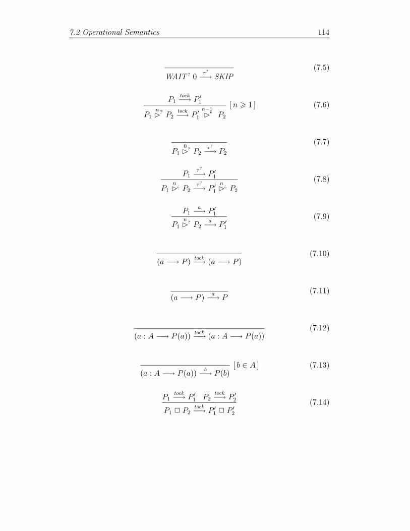
7.2 Operational Semantics 114
WAIT ? 0τ?
−→ SKIP(7.5)
P1tock−→ P ′
1
P1
n�
? P2tock−→ P ′
1
n−1�
∗ P2
[ n > 1 ] (7.6)
P1
0�
? P2τ?
−→ P2
(7.7)
P1τ?
−→ P ′1
P1
n�
¿ P2τ?
−→ P ′1
n�
¿ P2
(7.8)
P1a
−→ P ′1
P1
n�
? P2a
−→ P ′1
(7.9)
(a −→ P )tock−→ (a −→ P )
(7.10)
(a −→ P )a
−→ P(7.11)
(a : A −→ P (a))tock−→ (a : A −→ P (a))
(7.12)
(a : A −→ P (a))b
−→ P (b)[ b ∈ A ] (7.13)
P1tock−→ P ′
1 P2tock−→ P ′
2
P1 2 P2tock−→ P ′
1 2 P ′2
(7.14)

7.2 Operational Semantics 115
P1τ?
−→ P ′1
P1 2 P2τ?
−→ P ′1 2 P2
P2τ?
−→ P ′2
P1 2 P2τ?
−→ P1 2 P ′2
(7.15)
P1a
−→ P ′1
P1 2 P2a
−→ P ′1
P2a
−→ P ′2
P1 2 P2a
−→ P ′2
(7.16)
P1 u P2τ
−→ P1 P1 u P2τ
−→ P2
(7.17)
P1tock−→ P ′
1 P2tock−→ P ′
2
P1 ‖B
P2tock−→ P ′
1‖B
P ′2
(7.18)
P1µ
−→ P ′1
P1 ‖B
P2µ
−→ P ′1 ‖
B
P2
[ µ /∈ B, µ 6= X ] (7.19a)
P2µ
−→ P ′2
P1 ‖B
P2µ
−→ P1 ‖B
P ′2
[ µ /∈ B, µ 6= X ] (7.19b)
P1a
−→ P ′1 P2
a−→ P ′
2
P1 ‖B
P2a
−→ P ′1 ‖
B
P ′2
[ a ∈ B ] (7.20)
P1X
−→ P ′1
P1 ‖B
P2X
−→ P ′1
[X /∈ B ]P2
X−→ P ′
2
P1 ‖B
P2X
−→ P ′2
[X /∈ B ] (7.21)
P1tock−→ P ′
1 P2tock−→ P ′
2
P1 9 P2tock−→ P ′
1 9 P ′2
(7.22)
P1µ
−→ P ′1
P1 9 P2µ
−→ P ′1 9 P2
[ µ 6= X ] (7.23a)
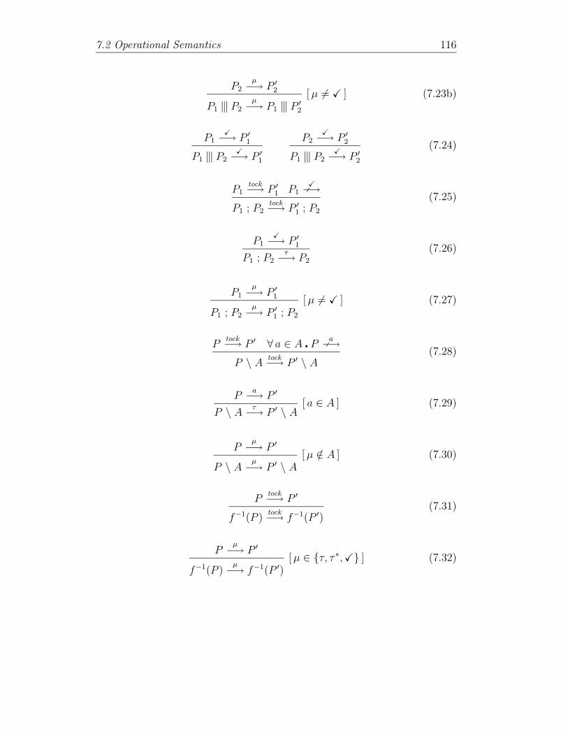
7.2 Operational Semantics 116
P2µ
−→ P ′2
P1 9 P2µ
−→ P1 9 P ′2
[ µ 6= X ] (7.23b)
P1X
−→ P ′1
P1 9 P2X
−→ P ′1
P2X
−→ P ′2
P1 9 P2X
−→ P ′2
(7.24)
P1tock−→ P ′
1 P1X
X−→
P1 ; P2tock−→ P ′
1 ; P2
(7.25)
P1X
−→ P ′1
P1 ; P2τ
−→ P2
(7.26)
P1µ
−→ P ′1
P1 ; P2µ
−→ P ′1 ; P2
[ µ 6= X ] (7.27)
Ptock−→ P ′ ∀ a ∈ A � P
aX−→
P \ Atock−→ P ′ \ A
(7.28)
Pa
−→ P ′
P \ Aτ
−→ P ′ \ A[ a ∈ A ] (7.29)
Pµ
−→ P ′
P \ Aµ
−→ P ′ \ A[ µ /∈ A ] (7.30)
Ptock−→ P ′
f−1(P )tock−→ f−1(P ′)
(7.31)
Pµ
−→ P ′
f−1(P )µ
−→ f−1(P ′)[ µ ∈ {τ, τ ∗,X} ] (7.32)

7.2 Operational Semantics 117
Pf(a)−→ P ′
f−1(P )a
−→ f−1(P ′)(7.33)
Ptock−→ P ′
f(P )tock−→ f(P ′)
(7.34)
Pµ
−→ P ′
f(P )µ
−→ f(P ′)[ µ ∈ {τ, τ ∗,X} ] (7.35)
Pa
−→ P ′
f(P )f(a)−→ f(P ′)
(7.36)
µX � Pτ
−→ P [(µX � P )/X].(7.37)
The remark made in Section 3.2 concerning negative premisses (appearingin Rules 7.25 and 7.28) applies here as well.
Note once again the one-to-one correspondence between these rules andthose associated with the operational semantics for MR and MTF .
The operational semantics enjoys a number of properties, which we listafter the following definitions.
If P is a closed node, we define initτUR
(P ) (initτ (P ) for short) to be theset of visible non-tock and silent events that P can immediately perform:
initτUR
(P ) = {µ ∈ ΣX ∪ {τ, τ ∗} | Pµ
−→}. We also write initUR(P ) to rep-resent the set of non-tock visible events that P can immediately perform:initUR(P ) = initτ
UR(P ) ∩ ΣX.
For P a closed node, we define an execution of P to be a sequence e =P0
x1−→ P1x2−→ . . .
xn−→ Pn (with n > 0), where P0 ≡ P , the Pi’s are nodes,
and each transition Pi
xi+1−→ Pi+1 in e is validly allowed by the operational
inference Rules 7.1–7.37. Here we have each xi ∈ ΣXtock
∪ {τ, τ ∗}. The set ofexecutions of P is written execUR(P ), or exec(P ) for short when no confusionis likely.
For P a closed node, the P -rooted graph, or labelled transition system,
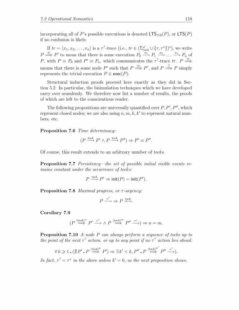
7.2 Operational Semantics 118
incorporating all of P ’s possible executions is denoted LTSUR(P ), or LTS(P )if no confusion is likely.
If tr = 〈x1, x2, . . . , xn〉 is a τ ?-trace (i.e., tr ∈ (ΣXtock
∪{τ, τ ∗})?), we write
Ptr
=⇒ P ′ to mean that there is some execution P0x1−→ P1
x2−→ . . .xn−→ Pn of
P , with P ≡ P0 and P ′ ≡ Pn, which communicates the τ ?-trace tr . Ptr
=⇒
means that there is some node P ′ such that Ptr
=⇒ P ′, and P〈〉
=⇒ P simplyrepresents the trivial execution P ∈ exec(P ).
Structural induction proofs proceed here exactly as they did in Sec-tion 5.2. In particular, the bisimulation techniques which we have developedcarry over seamlessly. We therefore now list a number of results, the proofsof which are left to the conscientious reader.
The following propositions are universally quantified over P, P ′, P ′′, whichrepresent closed nodes; we are also using n,m, k, k′ to represent natural num-bers, etc.
Proposition 7.6 Time determinacy:
(Ptock−→ P ′ ∧ P
tock−→ P ′′) ⇒ P ′ ≡ P ′′.
Of course, this result extends to an arbitrary number of tocks.
Proposition 7.7 Persistency—the set of possible initial visible events re-mains constant under the occurrence of tocks:
Ptock−→ P ′ ⇒ init(P ) = init(P ′).
Proposition 7.8 Maximal progress, or τ -urgency:
Pτ?
−→ ⇒ PtockX−→.
Corollary 7.9
(P〈tock〉n
=⇒ P ′ τ?
−→ ∧ P〈tock〉m
=⇒ P ′′ τ¿
−→) ⇒ n = m.
Proposition 7.10 A node P can always perform a sequence of tocks up tothe point of the next τ ? action, or up to any point if no τ ? action lies ahead:
∀ k > 1 � (@ P ′ � P〈tock〉k
=⇒ P ′) ⇒ ∃ k′ < k, P ′′ � P〈tock〉k
′
=⇒ P ′′ τ?
−→).
In fact, τ ? = τ ∗ in the above unless k′ = 0, as the next proposition shows.

7.2 Operational Semantics 119
Proposition 7.11 A state immediately reachable via a tock-transition can-not be fleetingly unstable:
Ptock−→ P ′ ⇒ P ′ τ
X−→.
Proposition 7.12 Finite variability—a program P ∈ TCSP cannot per-form unboundedly many actions within a finite number of tocks:
∀ k > 0 � ∃n = n(P, k) � ∀ tr ∈ (ΣXtock
∪ {τ, τ ∗})?�
(Ptr
=⇒ ∧ ](tr � tock) 6 k) ⇒ ]tr 6 n.
Note also that this formulation of finite variability implies Axiom UR7,via Theorem 7.13 below.
For A ∈ REF , we write P ref A if A = • ∨ (Pτ?
X−→ ∧ |A| ∩ init(P ) = ∅).We overload this notation by writing, for α ∈ URS , P ref α if
⋃{A | [A] in
α} = ∅ ∨ (Pτ
X−→ ∧⋃{A | [A] in α} ∩ init(P ) = ∅). Finally, for (α,A) ∈
RPAIR, we write P ref (α,A) if P ref α ∧ P ref A.
Any execution of a program P gives rise to a set of tests in a mannerconsistent with our understanding of instability. In detail, letting e be anexecution of P and u a test, we define inductively the relation e testU u byinduction on e:
P testU 〈(α,A)〉 ⇔ P ref (α,A)
(Pτ
−→)_e′ testU u ⇔ e′ testU u
(Pτ∗
−→)_e′ testU α glue u ⇔ P ref α ∧ e′ testU u
(Px
−→)_e′ testU 〈(α,A), x〉_u′ ⇔ x 6= τ ? ∧ P ref (α,A) ∧ e′ testU u′.
We can now define the function ΦUR, which extracts the denotationalrepresentation of a program from its set of executions.
Definition 7.2 For P ∈ NODER, we set
ΦUR(P ) = {u | ∃ e ∈ execUR(P ) � e testU u}.
The chief congruence result now reads:
Theorem 7.13 For any TCSP program P , we have
ΦUR(P ) = RUJP K.
The proof, while requiring a little more bookkeeping, follows the samepattern as that of Theorem 5.14, and is therefore omitted.

7.3 Refinement, Specification, Verification 120
7.3 Refinement, Specification, Verification
Let us conclude this chapter by saying a few words about specification sat-isfiability and verification. Much of our discussion on this topic in the caseof MR could be lifted directly to MUR, and it therefore seems unnecessaryto reproduce it here in great detail.
The nondeterministic refinement order can be defined on P(TESTU ) inthe expected manner:
Definition 7.3 For P,Q ⊆ TESTU (and in particular for P,Q ∈ MUR),we let P vUR Q if P ⊇ Q. For P,Q ∈ TCSP, we write P vUR Q to meanRUJP K vUR RUJQK, and P =UR Q to mean RUJP K = RUJQK.
We may drop the subscripts and write simply P v Q, P = Q whenever thecontext is clear.
This partial order naturally satisfies
P v Q ⇔ P u Q = P.
Specifications, of course, are assertions about processes, and behaviouralspecifications, such as process refinement, are specifications that are univer-sally quantified in the behaviours of the process. Behavioural specificationscan be identified with sets of tests, with a process meeting the specification ifit is a subset of it. Note that if a behavioural specification does not concernunstable refusals, Proposition 7.4 implies that it can simply be verified inMR.
Although we have not fully verified this, we strongly suspect, and willpresume, that MUR can be embedded into a domain in the same manner asMR, by dropping Axiom UR7. Consequently, a large class of behaviouralspecifications should be expressible as refinements; moreover, these shouldbe model checkable via the operational semantics using the algorithmic tech-niques which we describe in Appendix B.

Chapter 8
Timed Analysis (II)
We revisit some of the analysis carried out earlier in Chapter 6, and showthat MUR does circumvent, as claimed, certain of the problems we encoun-tered earlier. We concentrate exclusively on timed failure soundness, sincecompleteness, as well as the verification of specifications closed under inversedigitisation, were shown to be adequately handled within MR.
The main result of this chapter, Theorem 8.1, is interesting and valuablein that it confirms that refining timing granularity does lead to increasinglyand arbitrarily precise approximations of true continuous-time process be-haviour. This result does however come at a significant expense in modellingand algorithmic complexity and is likely to be less useful than the otherverification techniques described in Chapter 6.
8.1 Timed Denotational Expansion
We first define a timed denotational expansion function Expk : MUR −→P(TF ) which extends Chapter 6’s version of Expk in a manner consistentwith unstable refusal information.
The construction goes as follows. Let P ∈ MUR and let the test u =〈(α0, A0), a1, (α1, A1), a2, . . . , an, (αn, An)〉 belong to RUJP K. Let us writeeach αi as αi = [A1
i , A2i , . . . , A
ki
i ]. We first define preExpk(u) to be the set oftimed failures (s,ℵ) ∈ TF satisfying the following:

8.2 Timed Failure Soundness 122
∃(tji ∈ R+ | 0 6 i 6 n ∧ 0 6 j 6 ki), t0n+1 ∈ R+�
t00 = 0 ∧ t0n+1 = (1 + ](〈a1, a2, . . . , ai〉 � tock))/k ∧
(∀(i, j, l,m) � tji 6 tmi+l ⇔ l > 0 ∨ (l = 0 ∧ m > j)) ∧ tkn
n < t0n+1 ∧
s = 〈(t1, a1), (t2, a2), . . . , (tn, an)〉 \ tock ∧
(∀(1 6 i 6 n)�
ai = tock ⇒ (t0i = ](〈a1, a2, . . . , ai〉 � tock)/k ∧ tki−1
i−1 6= t0i )) ∧
ℵ ⊆n⋃
i=0
{ki−1⋃
j=0
{[tji , tj+1i ) × Aj+1
i } ∪ [tki
i , t0i+1) × |Ai|}.
We can now give
Definition 8.1 For any P ∈ MUR and k > 1, we define the timed denota-tional expansion Expk(P ) of P to be
Expk(P ) =⋃
{preExpk(u) | u ∈ P}.
(We will usually omit the subscript k when it is equal to 1.)
Note that the null refusal • is still treated as the empty refusal set.
8.2 Timed Failure Soundness
The timing inaccuracies pertaining to traces which we observed in Section 6.2naturally persist in the current setting. However, the problems having to dowith under-refusing events—which had ruled out any timed failure soundnessresult—have now vanished, thanks to unstable refusal information. As anillustration, consider once more the program
P = a1
−→ b.
We had observed that on the timed trace (0.7, a), the timed denotationalexpansion of RJP K was incapable of refusing b past time 1. However, the sit-uation is different with the timed denotational expansion of RUJP K: after thefirst tock , a τ ∗-transition is on offer, while b is robustly refused. Exp(RUJP K)will therefore have the behaviours (〈(0.7, a)〉, [0, t)), for all t < 2. (Note,however, that t is not allowed to equal 2, since the τ ∗-transition must occurstrictly before the second tock .) These behaviours certainly cover the timed

8.2 Timed Failure Soundness 123
failure (〈(0.7, a)〉, [0, 1.7)) ∈ FT JP K. And the corresponding test in RUJP K issimply 〈([], {b}), a, ([], {b}), tock , ([{b}], •)〉.
This situation is captured in general in Theorem 8.1, which we presentafter the following preliminaries.
Recall how the operational semantics for MUR is derived from the op-erational semantics for MR in such a way as to allow us to ‘keep track’ ofwhether nodes are in fleeting or robust states of instability (or, of course,in neither). This information is then encapsulated, respectively, in whethera node can perform τ -transitions or τ ∗-transitions (or neither). Naturally,the operational semantics for MTF can be altered in exactly the same way,by adopting precisely the same conventions as to the communications of τ ?
events as the operational semantics for MUR. Let us consider such an alteredoperational semantics for the remainder of this section.
One can then establish an analogue of Proposition 7.11, to the effectthat any state immediately reachable via an evolution cannot be fleetinglyunstable: for P, P ′ ∈ NODETF and t > 0,
Pt P ′ ⇒ P ′ τ
X−→.
The proof is a simple structural induction on P .
We have commented earlier how operational inference Rules 7.1–7.37 arein one-to-one correspondence with Rules 3.1–3.37. This naturally leads toa one-to-one correspondence between MUR-executions and normal MTF -executions. More precisely, this bijection takes a normal execution e =P0
z17−→ P1z27−→ . . .
zn7−→ Pn ∈ execTF (P ) to the execution e′ = P0x1−→
P1x2−→ . . .
xn−→ Pn ∈ execUR(P ), such that, for all 1 6 i 6 n, xi = tock whenzi7−→ =
1 , and xi = µ when
zi7−→ =µ
−→ (where µ ∈ ΣX ∪ {τ, τ ∗}).
Of course, we have, for any P ∈ MUR and k > 1, Exp(P ) = kExpk(P ).
We can now state:
Theorem 8.1 For any P ∈ TCSP and k > 1,
Expk(RUJkP K) vTF FT JP K.
Proof (Sketch.) As usual, it suffices to prove the result for k = 1.
Let P be fixed, and pick (s,ℵ) ∈ FT JP K. There is some execution e =P0
z17−→ P1z27−→ . . .
zn7−→ Pn ∈ execTF (P ) such that e fail (s,ℵ). Let e′ = [e]1

8.2 Timed Failure Soundness 124
be the lower digitisation of e, let e′′ be the normalisation of e′, and let o ∈execUR(P ) be the canonical execution corresponding to e′′. Let u ∈ RUJP Kbe a ≺-maximal test such that o testU u.
We have already seen, in Theorem 6.5, that s ∈ TTraces(preExp(u)). Wewould like to show that in fact (s,ℵ) ∈ preExp(u). We proceed as in thetimed trace case, and consider an arbitrary element (t, a) ∈ ℵ. We reason
that there must be Pkt′
Pk+1 in e such that dur(ek) 6 t, dur(ek) + t′ > t,
and Pka
X−→. (Here ek = P0z17−→ P1
z27−→ . . .zk7−→ Pk ≤ e represents the prefix
of e up to node Pk.) Under digitisation, the evolution Pkt′
Pk+1 becomes
P ′k
l P ′
k+1 in e′, with l ∈ N. Without loss of generality, let us assume thatl = 0 or l = 1, the second of which could be achieved via normalisation incase l > 1.
If l = 0, then dur(e′k) = [t]1 = dur(e′k+1). Since Pka
X−→ by assumption,
P ′k
aX−→, by the properties of digitisation. But init(P ′
k) = init(P ′k+1) by persis-
tency, and thus P ′k+1
aX−→. On the other hand, our earlier discussion lets us
conclude that P ′k+1 cannot be fleetingly unstable, i.e., P ′
k+1τ
X−→. It followsthat a must figure in the unstable refusal immediately following P ′
k+1, andtherefore that a is refusable from dur(e′k+1) = [t]1 to any time strictly lessthan dur(e′k+1) + 1 = [t]1 + 1. Naturally, this interval comprises t, whichentails that (t, a) is able to appear in the refusals of preExp(u).
If l = 1, then either [t]1 = dur(P ′k+1), in which case we repeat the above
argument, or [t]1 = dur(P ′k), in which case a is stably refused after P ′
k for upto one time unit. The result follows.
It is clear that this procedure can be carried out uniformly and con-currently for all (t, a) ∈ ℵ, as well as for the trace s. We conclude that(s,ℵ) ∈ preExp(u) ⊆ Exp(P ), as required. �
Theorem 8.1 is the timed failure soundness result which we had sought. Itinforms us that if some undesirable timed failure behaviour is ruled out by thedenotational expansion of RUJP K, then it is certainly not a possible behaviourof FT JP K. Together with quasi-completeness (Theorem 6.13, which can easilybe lifted to MUR), it allows us to ‘zero in’ on FT JP K by letting, if need be, kincrease. Eventual applications to specification verification would follow thesame pattern as in Chapter 6.

Chapter 9
Discussion, Comparisons,Future Work
The object of this thesis was to study the relationship between continuous-time and discrete-time models for timed process algebras, and to exploit thisrelationship towards applications, in particular model checking. Our mainaccomplishments are twofold: firstly, we have produced a stand-alone CSP-based discrete-time denotational model, equipped with a congruent opera-tional semantics, and compatible with the model checker FDR. Secondly, wehave linked this model to the standard continuous-time denotational and op-erational models for Timed CSP, and have shown how this connection couldbe exploited to reduce continuous-time verification problems to discrete-time,model checkable verification problems.
In greater detail, our work can be summarised as follows.
We introduced Timed CSP as our prototypical process algebra, togetherwith congruent continuous-time denotational and operational semantics, andestablished an important result, the digitisation lemma, which later allowedus to develop a powerful model checking technique with wide-ranging appli-cability.
We then discussed the principal issues pertaining to discrete-time mod-elling, and explained how the main difficulties could be overcome in certainmodels for untimed CSP.
We proceeded to carefully construct such a model, the discrete-time re-fusal testing model MR, offering congruent denotational and operationalsemantics which incorporated the properties previously identified. Refine-

9 Discussion, Comparisons, Future Work 126
ment, specifications and verification were discussed, and a model checkingalgorithm—presented in Appendix B—was described. We also remarked thatin the majority of the verification cases one was likely to meet in practice,the model checker FDR could be used directly.
We followed up with a chapter in which the exact links between thismodel and the continuous-time model MTF were studied, with once againan underlying emphasis towards verification. We discovered that the relation-ship between these continuous-time and discrete-time models for Timed CSPwas a very tight one, enabling us in a large number of instances to reduceverification problems in MTF to corresponding model checkable problemsin MR. More precisely, we built upon and later extended a result of Hen-zinger, Manna, and Pnueli’s to reduce specification satisfiability problemsfrom continuous-time to discrete-time, provided the specifications in ques-tion are closed under inverse digitisation. Since many specifications havethat property, this provided us with an efficient model checking algorithm,mentioned above, implementable on FDR in most cases. These results, whichconstitute the most important contribution of our work, were then illustratedin a simple railway level crossing case study. We also identified and discussedthe limitations of our discretisation approach.
A further chapter was devoted to constructing an extension of MR, thediscrete-time unstable refusal testing model MUR, to overcome certain short-comings of MR relating to unstable refusal information. Our treatment par-alleled that of MR, and we were able to show that MUR captured continuous-time behaviour more accurately and smoothly than MR. However it remainsto be shown how substantial the eventual practical benefits of this observa-tion will prove to be.
We elected to focus on Timed CSP for a number of reasons. Firstly,Timed CSP comes endowed with continuous-time denotational and opera-tional semantics, has been the focus of a considerable body of previous work,and is a natural extension of (untimed) CSP. The latter, of course, has beeneven more widely studied and is equipped with denotational, operational,and algebraic semantics, as well automated model checking tools. The com-bination of Timed and untimed CSP therefore seemed likely to be a fertileterrain in which to conduct our investigations.
Secondly, Timed CSP possesses a large number of the properties andcharacteristics usually found in other timed process algebras. The robustnessof the methods used in our analysis makes it very plausible that our resultsshould apply to a wide range of similar process algebras, as well as to anumber of proposed extensions and variants of Timed CSP, discussed below.

9 Discussion, Comparisons, Future Work 127
Lastly, denotational CSP-based models typically have an internal speci-fication mechanism rooted in refinement. This allowed us to avoid having tointroduce an independent formal specification formalism, such as temporallogic, and concentrate instead on the task at hand. Handling specificationsvia refinement has the additional appeal of being much closer to the top-downapproach usually adopted in system design and implementation; refinement-based formal methods are consequently more likely to prove useful through-out a project’s production cycle. Temporal-logic-based formalisms, on theother hand, can be more flexible (enabling one, for example, to express as-sertions about internal state variables), and can be studied independently ofany model, making them more portable. For an in-depth account of the useof temporal logics in Timed and untimed CSP, we refer the reader to [Jac92].
A number of continuous-time process algebras other than Timed CSP ap-pear in the literature. These include the algebras of [Wan91, Che92], whichare timed extensions of CCS [Mil89], and predicated upon an operationalsemantics which uses strong bisimulation for process equivalence. In [BB91],Baeten and Bergstra combine a similar approach together with a congruentcomplete algebraic semantics, while Gerth and Boucher [GB87] complementtheir operational semantics with a timed-failures-based denotational seman-tics similar to that of MTF . A more abstract denotational model, subsumingtimed failures, is offered in [Jef91a], once again together with a congruentoperational semantics.
Discrete-time process algebras have also been widely studied. In [MT90,NS94, CLM97], we find process algebras rooted in operational semantics andstrong bisimulation, whereas the process algebra of [HR91] uses instead anoperational semantics in which testing equivalence defines the notion of equal-ity between processes. Jeffrey [Jef91b] proposes a process algebra incorpo-rating infinite nondeterminism and Zeno processes, rooted in a failures-baseddenotational semantics, and equipped with a congruent complete algebraicsemantics. Naturally, some of the continuous-time process algebras notedabove also have discrete-time interpretations.
Although these lists are far from exhaustive, they give an idea of therange of alternative process algebraic formalisms available in the literature.More thorough overviews can be found in [NS91, Sch95, Ver97].
The discrete-time models which we have constructed in this thesis buildupon ideas appearing in [RR86, RR87, Ree88, RR99, Phi87, Muk93, Ros97](on the denotational side), and [Sch95, NS91, NS94] (on the operationalside). Denotationally, MR and MUR share a number of characteristics withJeffrey’s model for Discrete timed CSP [Jef91b].

9 Discussion, Comparisons, Future Work 128
Other formalisms for modelling timed systems include timed transitionsystems [HMP90], timed graphs [ACD90, ACD93], timed automata [AD94],hybrid systems [NOSY93, Hen96, HHWT97], etc. Unlike process algebras,these tend to be intrinsically rooted in state-based models, and are usuallycloser to the implementation level. One could argue that process algebras,being more abstract, are more versatile and better suited to algebraic andmodular (i.e., compositional) reasoning, while retaining state-based inter-pretations via their operational semantics (together with, if need be, con-gruence theorems). On the other hand, the price paid for this higher levelof abstraction is often a significant overhead in rigorously establishing cer-tain operational properties of processes—cf., for instance, the proofs of thedigitisation lemma or finite variability. One is also sometimes faced with un-wanted phenomena which are not always easy—if at all possible—to get ridof, such as Zeno behaviours, divergence, point nondeterminism, unboundednondeterminism, and so on.
One of the earliest attempts to discretise continuous-time models witha view towards verification was the technique of timewise refinement, in-troduced in [Ree88, Ree89] and developed in [Sch89, RRS91, Sch97]. Thismethod is essentially a translation from Timed to untimed CSP which dropsall timing information, retaining only (and loosely) the relative order in whichevents occur. Although of course not suitable for every verification purpose,timewise refinement, when applicable, is a spectacularly economical prooftechnique, often able to handle problems for which it is not computationallyfeasible to apply straightforward model checking algorithms.
Alur, Courcoubetis, and Dill’s seminal work on region graphs [ACD90,ACD93] provided the first algorithm to model check (continuous-time) timedgraphs with respect to satisfiability of formulas expressed in the temporallogic TCTL. Timed graphs consist of a finite set of nodes together with afinite set of real-valued clocks, giving rise to an uncountable number of states.However, Alur et al. showed that it was possible to construct an equivalencerelation on the state space, partitioning it into a finite number of regions,in such a way that no TCTL formula can distinguish states belonging tothe same region. This led naturally to a model checking algorithm. Thetechnique is however computationally expensive—deciding satisfiability ofTCTL formulas by timed graphs can be shown to be PSPACE-complete—and much subsequent research has concentrated on finding ways to curb theresulting complexity [HNSY94, LL95, SS95, HKV96, HK97].
Jackson [Jac92] showed how to apply the region graphs algorithm in thetimed failures model for a restricted subset of Timed CSP. The idea es-
9 Discussion, Comparisons, Future Work 129
sentially consists in curtailing Timed CSP syntax, yielding the sub-process-algebra FTCSP, all of whose programs can then be translated into equivalenttimed graphs. (Going in the other direction, the constructions of [CG95] in-dicate how to translate timed automata into Timed CSP—the latter is thusat least as expressive as the former.)
According to Cook’s thesis, the problem of deciding satisfiability of TCTLformulas by timed graphs, being PSPACE-complete, is ‘intractable’. How-ever, in many practical cases the actual complexity turns out to be manage-able, for two reasons. The first is that the systems in which we tend to beinterested often exhibit symmetry and regularity, which significantly reducesthe complexity. The second reason is that, even though the equivalence re-lation associated with region graphs cannot be made any coarser if arbitraryTCTL formulas are considered, in many cases (such as reachability analy-sis, or specifications that are closed under inverse digitisation), verifying thespecification in question does not necessarily require the full discriminativepower of regions, consequently reducing the complexity. This has been ex-ploited, among others, in [BSV95], leading to a general technique of iterativerefinement which could easily also be employed in our setting.
We will not give a precise and comprehensive account of how the workcarried out in this thesis compares with region graphs, as such an accountwould have to be quite lengthy. However, a rough overview can be offered asfollows. Each parallel component of a compound system has a clock associ-ated to it. Regions are then basically constructed by comparing respectivelythe integral and fractional parts of these clocks, where for fractional partsthe allowable comparison predicates are equality with zero, equality, and lessthan. In our setup, on the other hand, our use of the tock event faithfullycaptures the integral part of a single clock, and furthermore any subsequentinformation concerning the clock’s fractional part can only be expressed interms of a single predicate, less than or equal to. It follows that the equiva-lence relation which this induces on the state space is much coarser than thatof region graphs, with the twin corollaries that the analysis offered within ourframework should be computationally more efficient than full-fledged regiongraphs algorithms, but may also occasionally fail to produce an answer insituations where a region graphs investigation would be successful. This be-ing said, we recall that, by refining the time granularity of the discrete-timeinterpretations of programs, increasing precision can be achieved. We shallreturn to this question shortly.
In [HMP92], Henzinger et al. address the important question of whichdense-time properties can be investigated with integral-time methods, and

9 Discussion, Comparisons, Future Work 130
how. They carry out their work in the realm of timed transition systems,together with the temporal logic MTL. We have used one of their mainresults—Theorem 6.8, dealing with timed traces—which we later extendedin Theorem 6.15 to incorporate timed failures. We then built on these resultsto produce the central Theorems 6.10 and 6.16 and Corollaries 6.11 and 6.17,allowing us to reduce the verification of any specification closed under inversedigitisation to our discrete-time setting.
Much research has gone into temporal logics and their relation to modelchecking. Excellent and thorough accounts can be found in [HMP90, AH93,AH94, Hen98]. In [HK97], Henzinger and Kupferman show that model check-ing TCTL formulas can be carried out on any tool which allows CTL modelchecking. As they point out, since such tools are typically much more so-phisticated (not to mention widespread) than TCTL model checkers, thisreduction amounts to more than just an interesting theoretical result. Like-wise, an advantage of the work which we have carried out is that efficient andcompetitive model checking tools such as FDR can (in most cases) directlybe employed to verify specifications on Timed CSP processes.
An interesting distinctive approach to using temporal logics towards ver-ification has been the development of TLA and TLA+, together with themodel checker TLC [YML99]. Rather than expressing system and specifi-cation using two different formalisms (such as timed graphs and temporallogic), the idea here is to translate the system itself into the temporal logicTLA+, the very language used to express specifications. The satisfiabilitycheck is then carried out entirely within a single temporal logic framework.(This approach is in some sense dual to ours, where system and specificationare both expressed as processes, with satisfiability corresponding to refine-ment.)
Symbolic model checking and related techniques have attracted muchattention in recent years. Examples include [BCM+92], using binary de-cision diagrams, [BLP+99], introducing clock difference diagrams, a timedanalogue of binary decision diagrams, [HNSY94, NOSY93], focussing on hy-brid systems, and [HKV96, AHR98], focussing on dense-time timed transi-tion systems. Other formal methods include proof systems [Sch89, Dav91,Sch94], property preserving abstractions [LGS+95], and applications of data-independence [Laz99]. Whether and how such techniques can be adapted toour framework are very interesting and relevant research questions.
Let us now consider in turn a number of avenues along which our frame-work could be extended, and discuss other opportunities for future research.

9 Discussion, Comparisons, Future Work 131
An intrinsic limitation of the original formulation of CSP and TimedCSP has to do with the need for the environment to cooperate on all events.Although this difficulty can usually be circumvented in practice, as we arguebelow, it does lead to unnatural situations. As pointed out by Davies [Dav91],not all events are appropriately modelled as synchronisations: a telephonemay ring, for instance, even if no-one is prepared to actively participate inlistening to it.1 However it is impossible in Timed CSP to describe a systemin which, for example, the event SprinklerOn is guaranteed to occur at most5s after the event FireAlarm is observed; in general it is even impossible toguarantee that events occur as soon as they become available.
Current solutions to this problem fall in three categories. The first isto bypass the need for environmental cooperation by hiding the event inquestion, as we did in our railway level crossing example (Section 6.7) toensure that cars drove off the dangerous crossing after exactly 10s. Un-fortunately, such events, being hidden, can then by definition no longer beobserved. A second, more sophisticated solution is to postulate an assume-guarantee framework, which lets us draw appropriate conclusions, or guar-antees, from environmental assumptions; this is discussed, among others, in[KR91, Dav91], and applied in [Sch94]. From a model checking perspective,a possible implementation could consist in ascribing a certain priority to suchevents to ensure that time cannot pass while they are on offer. The thirdand most radical option is to redesign the semantic models to incorporatebroadcast concurrency, or signals, as is done in [Dav91]. We expect thatany of these approaches would successfully mesh with the relatively robustconstructions and techniques described in this thesis.
Another point worth addressing is the extent to which we can push theparadigm of specification-as-refinement in Timed CSP, and how it compareswith temporal logic, particularly in terms of expressiveness. This difficult is-sue is obviously very important, given the nature of our denotational modelsas well as the mode of operation of FDR, if we are serious about applyingour efforts to real-world problems. As we have seen, the main difficultiesstem from the fact that Zeno behaviours and unrestricted unbounded non-determinism sit uneasily with our denotational semantics (particularly incontinuous time). We have argued that it is not Zeno behaviours per se thatare problematic, but the fact that they potentially lead to divergence underhiding. Of course, the fact that our models are predicated upon ultrametricspaces and invoke the contraction mapping theorem to compute fixed points
1Then again... This echoes the age-old metaphysical query, “if a tree falls in a forestwith no-one nearby, does it make a noise?”

9 Discussion, Comparisons, Future Work 132
means that some definite work will be required to integrate Zeno featuresinto the denotational semantics. A starting point seems to lie in the factthat our discrete-time models have alternative cpo-based constructions.
An interesting question is whether our discrete-time model MR is canon-ical in any way; i.e., whether it is the most abstract model with respect tosome outside criterion, such as some testing equivalence, or the verification ofspecifications that are closed under inverse digitisation. As far as the secondcriterion is concerned, Proposition 6.18 hints strongly that the answer isnegative. Steve Schneider has suggested a discrete-time model similar toMR but with refusals recorded only prior to tock events. It seems that itshould be possible to build such a model and employ it as we have MR toverify exactly specifications closed under inverse digitisation. Moreover, webelieve that such a model would in fact be fully abstract with respect to thiscriterion. Since this model would clearly be coarser than MR, it is naturalto believe that its corresponding model checking algorithm should be moreefficient than MR’s as well.
On the other hand, we have seen that MR can be used to verify exactlycertain specifications that are not closed under inverse digitisation. Canwe characterise these specifications? Can we characterise specifications, orperhaps processes, that are closed under inverse digitisation?2
Another interesting research direction is to look for less abstract modelsthan MR, together with correspondingly larger natural classes of specifica-tions that such models could verify exactly. Bill Roscoe in particular hassuggested a model similar ro MR but with the tock event split into two ‘si-multaneous’ sub-events, representing respectively the beginning and the endof a standard tock . In this way, it would be possible to determine whetherother events occur strictly before, at the same time as, or strictly after tock .It seems clear that such a model would induce a finer equivalence than MR
on the continuous-time state space of processes, although it would clearlynot correspond to the still finer equivalence of region graphs. Whether thelatter equivalence can be captured in a discretisation framework is a veryinteresting question, the answer to which we believe to be negative. (By“discretisation” we essentially mean discrete-time modelling in which time isrepresented via a single fictitious digital clock.) In support of our negativeconjecture, note that, according to Proposition 6.22, there are specificationswhich fail to become closed under inverse digitisation at any level of timing
2In [HMP92], Henzinger et al. offer sufficient criteria for a specification to be closedunder inverse digitisation, but there is no suggestion that these criteria are in fact neces-sary.

9 Discussion, Comparisons, Future Work 133
granularity. This also suggests that it is impossible to obtain a discrete-timemodel in which every refinement-based Timed CSP specification can be ver-ified exactly. We believe all these questions to be very interesting and wellworthy of further research.
A difficult problem seems to be the development of an algebraic seman-tics for Timed CSP. Propositions 6.19 and 6.20 imply that MTF and MR
would actually have to have different such semantics. Unfortunately, defin-ing a suitable notion of normal form seems complicated since any normalform would necessarily have to incorporate parallel operators, in view ofProposition 6.23.3 An interesting question is whether there is a good in-herent notion of minimal degree of parallelism for timed processes (per-haps related to minimal sets of clocks in corresponding timed automata—see[ACH94, KR96, CG95]). As a related note, we point out that all the “lawsof Timed CSP” listed in [RR99] can easily be shown to hold in each of MTF ,MR, and MUR (with δ = 0).
Full abstraction has been discussed earlier with respect to criteria suchas the verification of specifications that are closed under inverse digitisation.A dual concern is that of the density of the denotational image of the setTCSP of programs in the denotational model (whether MTF or MR). Toour knowledge, very little work has been carried out in this direction in thepast (in the case of MTF ), which suggests that it is not easy to identifyan adequately constraining set of axioms. For example, a process such asP = WAIT 0.5 could not, in our syntax, be reached as the limit of a sequenceof TCSP programs (with respect to the standard ultrametric on MTF ). Notehowever that P satisfies Axioms TF1–TF5, i.e., P is a bona fide element ofMTF . A solution could be to ban P by imposing the digitisation lemma asa sixth axiom. Would there then still be MTF processes which could notbe approximated by TCSP programs? And if so, can one find a sufficientlyconstraining set of axioms that would achieve density of TCSP? Thesequestions, of course, can also be asked of MR and MUR. We remark, while onthe topic, that there is no particular reason to prefer to enunciate propertiessuch as Axioms R1–R8 as axioms rather than establish them as propositions,other than to derive a density result of the type described above. In fact,as we saw in the proof of the congruence theorem for MR, there is probablyless work to do if one has as few axioms to start with as possible.
A rather deep and difficult problem in Timed CSP concerns the studyof nondeterminism, particularly in the continuous-time case (see [RR99]).
3Schneider’s ‘head standard form’ [Sch92] incorporates unbounded nondeterministicchoice as well as a generalised prefix operator, neither of which are allowed in our syntax.

9 Discussion, Comparisons, Future Work 134
It is interesting to ask whether these questions could be clarified via thelinks between the continuous-time and discrete-time models. For instance, isdeterminism an invariant whether a process is interpreted in MTF or MR?The answers to such questions potentially have important applications to thestudy of non-interference in computer security [Ros95]. This is a researchprogramme which we are already involved in.
Throughout this work, we have exclusively been concerned with the timedfailures model MTF . One possible extension would be to move over to themore sophisticated timed failures-stability model MTFS [RR99], able to han-dle ‘global’ stability (invariance with respect to the passage of time). Thebedrock of our constructions and analyses has lain in having a congruent op-erational semantics complementing our denotational continuous-time model,together with an appropriate digitisation lemma. The first of these (in thecase of MTFS ) is achieved in Appendix C, and we are confident that thesecond should easily follow.
A further extension could be the inclusion of fairness. A traditional solu-tion to this problem is achieved via infinite traces models (see, e.g., [Ros97]),which for obvious reasons are not an ideal framework for model checking.A less subtle, but more forcible approach consists in prioritising events, forexample by lowering the priority of certain events if they are seen to occur‘a lot’. As we have seen, achieving priority in our models, which allowed usto implement maximal progress, is not difficult. The framework could easilybe extended and authoritarian renditions of fairness subsequently enacted.
Another possibility could be the addition of functional programming ca-pabilities to the syntax, as is done for instance in [Laz99] in untimed CSP.
A much more ambitious, if speculative, extension would see the incor-poration of probability to the framework. A good starting point might be[Low95].
We conclude by pointing out that, however interesting the theoreticalresults and speculations we have presented here are, it would also certainlybe desirable to apply them to a number of case studies and find out exactlyhow closely theory matches practice.

Appendix A
Mathematical Proofs
A.1 Proofs for Chapter 3
Lemma A.1 (3.11) Let P ∈ TCSP, and let e = P0z17−→ P1
z27−→ . . .zn7−→
Pn ∈ execTF (P ). For any 0 6 ε 6 1, there exists an execution [e]ε = P ′0
z′17−→
P ′1
z′27−→ . . .z′n7−→ P ′
n ∈ execTF (P ) with the following properties:
1. The transitions and evolutions of e and [e]ε are in natural one-to-one
correspondence. More precisely, whenever Pi
zi+17−→ Pi+1 in e is a tran-
sition, then so is P ′i
z′i+17−→ P ′
i+1 in [e]ε, and moreover z′i+1 = zi+1. On
the other hand, whenever Pi
zi+17−→ Pi+1 in e is an evolution, then so is
P ′i
z′i+17−→ P ′
i+1 in [e]ε, with |zi+1 − z′i+1| < 1.
2. All evolutions in [e]ε have integral duration.
3. P ′0 ≡ P0 ≡ P ; in addition, P ′
i ∈ TCSP and initTF (P ′i ) = initTF (Pi) for
all 0 6 i 6 n.
4. For any prefix e(k) = P0z17−→ P1
z27−→ . . .zk7−→ Pk of e, the corresponding
prefix [e]ε(k) of [e]ε is such that dur([e]ε(k)) = [dur(e(k))]ε.
We present the proof after a number of preliminaries.
We first define an operational analogue to the notion of semantic binding.A syntactic binding is a function η : VAR −→ NODETF . Any open node Ptogether with a syntactic binding η give rise to a closed node Pη via sub-stitution in the obvious way. We also have standard operations on syntactic
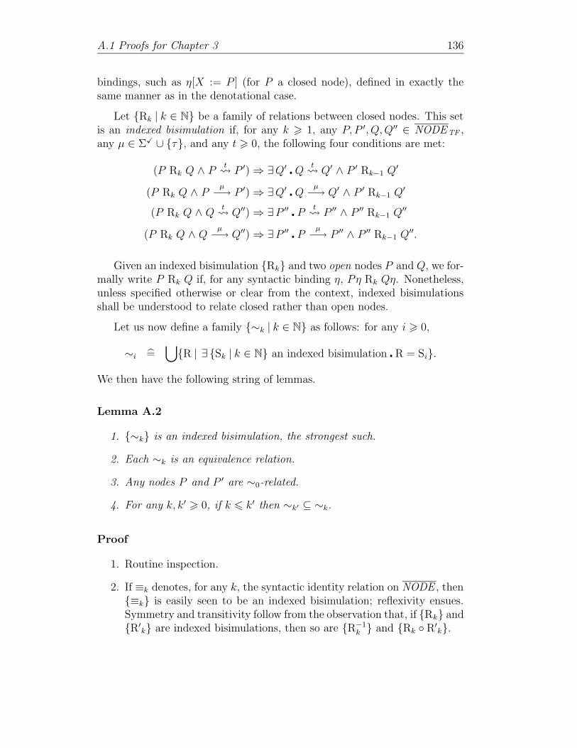
A.1 Proofs for Chapter 3 136
bindings, such as η[X := P ] (for P a closed node), defined in exactly thesame manner as in the denotational case.
Let {Rk | k ∈ N} be a family of relations between closed nodes. This setis an indexed bisimulation if, for any k > 1, any P, P ′, Q,Q′′ ∈ NODETF ,any µ ∈ ΣX ∪ {τ}, and any t > 0, the following four conditions are met:
(P Rk Q ∧ Pt P ′) ⇒ ∃Q′ �Q
t Q′ ∧ P ′ Rk−1 Q′
(P Rk Q ∧ Pµ
−→ P ′) ⇒ ∃Q′ �Qµ
−→ Q′ ∧ P ′ Rk−1 Q′
(P Rk Q ∧ Qt Q′′) ⇒ ∃P ′′ � P
t P ′′ ∧ P ′′ Rk−1 Q′′
(P Rk Q ∧ Qµ
−→ Q′′) ⇒ ∃P ′′ � Pµ
−→ P ′′ ∧ P ′′ Rk−1 Q′′.
Given an indexed bisimulation {Rk} and two open nodes P and Q, we for-mally write P Rk Q if, for any syntactic binding η, Pη Rk Qη. Nonetheless,unless specified otherwise or clear from the context, indexed bisimulationsshall be understood to relate closed rather than open nodes.
Let us now define a family {∼k | k ∈ N} as follows: for any i > 0,
∼i =⋃
{R | ∃ {Sk | k ∈ N} an indexed bisimulation � R = Si}.
We then have the following string of lemmas.
Lemma A.2
1. {∼k} is an indexed bisimulation, the strongest such.
2. Each ∼k is an equivalence relation.
3. Any nodes P and P ′ are ∼0-related.
4. For any k, k′ > 0, if k 6 k′ then ∼k′ ⊆ ∼k.
Proof
1. Routine inspection.
2. If ≡k denotes, for any k, the syntactic identity relation on NODE , then{≡k} is easily seen to be an indexed bisimulation; reflexivity ensues.Symmetry and transitivity follow from the observation that, if {Rk} and{R′
k} are indexed bisimulations, then so are {R−1k } and {Rk ◦ R′
k}.

A.1 Proofs for Chapter 3 137
3. If we let R0 = NODE × NODE , and let, for any k > 1, Rk = ∅, weeasily find that {Rk} is an indexed bisimulation. The result follows bymaximality of {∼k}.
4. For any k > 0, let Rk =⋃{∼i | i > k}. One easily verifies that {Rk} is
an indexed bisimulation, and thus that Rk ⊆ ∼k for any k; the resultfollows.
�
If η and η′ are syntactic bindings and k ∈ N, let us write η ∼k η′ if, forall X ∈ VAR, η(X) ∼k η′(X). We then have:
Lemma A.3 Let P ∈ NODE and η ∼k η′ for some syntactic bindings η, η′,and some fixed k > 0. Then Pη ∼k Pη′.
Proof (Sketch.) We proceed by induction on k. For a given k, we define afamily {≈n} as follows: for n 6 k, ≈n = {(Rρ,Rρ′) |R ∈ NODE ∧ ρ ∼n ρ′}.And for n > k, ≈n = ∅. We remark that the definition of ≈i, for any fixed i,is uniform over all k > i.
We aim to show that, for any particular value of k, {≈n} is an indexedbisimulation. By the previous lemma, this will entail that any pair of nodesthat are ≈i-related are in fact ∼i-related. The result will then follow bychoosing i = k, P = R, ρ = η, and ρ′ = η′.
The base case k = 0 is trivial: {≈n} is clearly—in fact, vacuously—anindexed bisimulation.
For the induction step (k + 1), we proceed by structural induction onR. We need to show that, whenever Rρ ≈n Rρ′, Rρ and Rρ′ satisfy theconditions for {≈n} to be an indexed bisimulation.
The structural induction cases are fairly easy. We tackle parallel compo-sition and recursion in illustration:
Let R = R1 ‖ R2. We assume that ρ ∼k+1 ρ′ (for greater values of nthan k + 1 the result vacuously holds, and for lesser values the result followsby the induction hypothesis on k) and thus that Rρ ≈k+1 Rρ′. Supposethat Rρ
a−→ Q, for some a ∈ ΣX. Since Rρ ≡ (R1 ‖ R2)ρ ≡ R1ρ ‖ R2ρ,
we find, according to the operational rules of inference, that we must haveR1ρ
a−→ Q1, R2ρ
a−→ Q2, and Q ≡ Q1 ‖ Q2.
By the structural induction hypothesis, since R1ρa
−→ Q1, it must be thecase that R1ρ
′ a−→ Q′
1, with Q1 ≈k Q′1. We can now invoke the induction

A.1 Proofs for Chapter 3 138
hypothesis on k to conclude that Q1 ∼k Q′1. Likewise, since R2ρ
a−→ Q2, it
must be the case that R2ρ′ a−→ Q′
2, with Q2 ∼k Q′2.
Write Q′ ≡ Q′1 ‖ Q′
2. It is clear that Rρ′ a−→ Q′.
Now define syntactic bindings ν and ν ′ as follows: ν and ν ′ agree on allvariables other than X and Y , and ν(X) = Q1, ν(Y ) = Q2, ν ′(X) = Q′
1, andν ′(Y ) = Q′
2. Clearly, ν ∼k ν ′. We have
Q ≡ Q1 ‖ Q2 ≡ (X ‖ Y )ν ≈k (X ‖ Y )ν ′ ≡ Q′1 ‖ Q′
2 ≡ Q′
as required.
The other cases (τ -transitions, evolutions, and symmetry) are entirelysimilar.
We now consider the case of recursion (in our structural induction).
Note that (µX � R)ρτ
−→ R[µX � R/X]ρ and likewise (µX � R)ρ′ τ−→
R[µX �R/X]ρ′ (and these are the only allowable behaviours). But if ρ ∼k+1 ρ′
(as we are assuming), then ρ ∼k ρ′ (as per Lemma A.2), and we are done:R[µX �R/X]ρ ≈k R[µ X �R/X]ρ′, as required. �
The following result will not directly be needed elsewhere in this work,but has been included because of its independent central importance in oper-ational semantics, and because its proof is now only a small step away fromthe results already contained in this section.
Proposition A.4 For any k > 0, ∼k is a congruence over Timed CSPsyntax. In other words, all Timed CSP operators are preserved by ∼k.
Proof (Sketch.) One proceeds by case analysis, considering each TimedCSP operator in turn. The result is trivial in the case of nullary operators.For binary operators, and unary operators other than recursion, the argumentis reasonably straightforward; we consider the case of external choice as anillustration. We then conclude by tackling recursion.
Let P ≡ P1 2 P2 and Q ≡ Q1 2 Q2, where for simplicity we are onlyconsidering closed nodes. Suppose that P1 ∼k Q1 and P2 ∼k Q2. We claimthat P ∼k Q follows. To see this, define, for any n > 0,
≈n = ∼n ∪ {(R1 2 R2, S1 2 S2) | R1 ∼n S1 ∧ R2 ∼n S2}.
It now clearly suffices to show that {≈n} is an indexed bisimulation. Thisis a simple inspection. For instance, suppose that R ≈n S for some n > 1.

A.1 Proofs for Chapter 3 139
If this is already an instance of ∼n, we are done. Otherwise, we must haveR ≡ R1 2 R2 and S ≡ S1 2 S2, with R1 ∼n S1 and R2 ∼n S2. Nowconsider the various transitions and evolutions available to R. For example,
suppose that (R1 2 R2)t R′, for some some t > 0. Consulting the rules
of inference, we conclude that it must have been the case that R1t R′
1,
R2t R′
2, and R′ ≡ R′1 2 R′
2. Since R1 ∼n S1, we must have S1t S ′
1 forsome node S ′
1 with R′1 ∼n−1 S ′
1. Likewise, there must be some node S ′2 such
that S2t S ′
2 and R′2 ∼n−1 S ′
2. Writing S ′ ≡ S ′1 2 S ′
2, it then follows that
(S1 2 S2)t S ′ and that R′ ≈n−1 S ′. Other cases are equally easy; {≈n} is
therefore a time-bisimulation, as required.
The recursion operator is handled by induction on k. Specifically, weshow that, for any P,Q ∈ NODE , P ∼k Q implies that µX � P ∼k µX �Q.
The base case (k = 0) is trivial. For the induction step, we consider opennodes P and Q such that P ∼k+1 Q. Since this entails that P ∼k Q (asper Lemma A.2), we can invoke the induction hypothesis to conclude thatµX � P ∼k µX �Q. We must show that in fact µX � P ∼k+1 µX �Q.
Let η be some fixed syntactic binding. We have (µX � P )ητ
−→ P [µX �P/X]η ≡ Pη[X := (µX �P )η]. Likewise, (µX �Q)η
τ−→ Qη[X := (µX �Q)η].
So we need to show that Pη[X := (µX � P )η] ∼k Qη[X := (µX �Q)η]. ButPη[X := (µX � P )η] ∼k Pη[X := (µX �Q)η] by Lemma A.3, since we knowthat µX �P ∼k µX �Q. And by definition, Pη[X := (µX �Q)η] ∼k Qη[X :=(µX �Q)η], since P ∼k Q. The result follows by transitivity of ∼k. �
Proposition A.4 easily entails that strong bisimilarity (cf., for example,[Mil89]) is a congruence for Timed CSP. This remains true even in non-finitely branching operational semantics, although in that case one must useordinals in indexed bisimulations rather than simply positive integers. Weend our digression here and now return to our main thread.
Let P ∈ NODE , and let η be a syntactic binding. We define a functionF = FP,X,η : NODE −→ NODE , as follows: F (Q) = (SKIP ; P )[Q/X]η. Inessence, FP,X,η mimics the unwinding of recursion in P over the variable X,under the binding η, and then substitutes its argument for all free instancesof X in P . This leads to the following:
Lemma A.5 Let P ∈ NODE and let η be a syntactic binding. For anyk ∈ N, F k(STOP) ∼k (µX � P )η, where F = FP,X,η is as above.
Proof We proceed by induction on k. The base case k = 0 is trivial since,

A.1 Proofs for Chapter 3 140
according to Lemma A.2, all programs are ∼0-related. For the inductionstep, we first make the simple observations that, for any nodes R and R′, ifR ∼k R′ then (SKIP ; R) ∼k+1 (SKIP ; R′), as an immediate calculation ofthe possible executions easily reveals.
So assume that the result holds for k. We have the following sequence ofdeductions, select justifications of which follow.
F k+1(STOP) ≡ F (F k(STOP))
≡ (SKIP ; P )[F k(STOP)/X]η
≡ SKIP ; (P [F k(STOP)/X]η)
≡ SKIP ; (P (η[X := F k(STOP)]))
∼k+1 SKIP ; (P (η[X := (µX � P )η])) (1)
≡ SKIP ; (P [(µX � P )η/X]η)
∼k+1 (µX � P )η. (2)
This concludes the induction step. (1) follows from our earlier observationtogether with Lemma A.3, using the fact that F k(STOP) ∼k (µX � P )η bythe induction hypothesis. (2) rests on the observation that SKIP ; (P [(µX �P )η/X]η) ∼n (µX � P )η for any n > 0, as a straightforward calculation willattest. �
Lemma A.6 Let P,Q ∈ NODE, k > 1, and suppose that P ∼k Q. Then,for any execution e = P0
z17−→ P1z27−→ . . .
zn7−→ Pn of P with n < k, there is acorresponding execution u = Q0
z17−→ Q1z27−→ . . .
zn7−→ Qn of Q, with identicaltransitions and evolutions, and such that, for all 0 6 i 6 n, init(Pi) =init(Qi).
The executions e and u are said to be bisimilar.
Proof (Sketch.) This is a routine induction on n; the inductive statementis strengthened to require that Pi ∼k−i Qi, for all i. �
We can now give the proof of Lemma A.1.
Proof Let us agree that programs satisfying the conclusion of the lemmabe termed digitisable. Recall also that, given an execution e and a pivot ε asin the lemma statement, the execution [e]ε is called the ε-digitisation of e.
We proceed by structural induction on P , as follows: for any syntacticbinding η such that η(X) is a digitisable TCSP program for all X ∈ VAR,

A.1 Proofs for Chapter 3 141
we claim that Pη is digitisable as well. Here P ∈ TCSP, and in particularonly contains integral delays. The principal cases are presented below.
case WAIT n: The result follows easily from the fact that n is an integer.
case a −→ P : Let e be an execution of (a −→ P )η ≡ a −→ Pη, and let ε befixed. If e is either trivial or begins immediately with an a-transition,the result follows by the induction hypothesis. On the other hand, astring of initial evolutions give rise to no greater difficulties, thanksto Rule 3.10, than a single initial evolution; thus let us assume for
simplicity that e = (a −→ Pη)t (a −→ Pη)
a−→ e′, where e′ ∈
exec(Pη).
Writing again t to designate the fractional part of t, we now apply theinduction hypothesis to P , with syntactic binding η, execution e′, andpivot ε′ = ε − t + [t]ε, to get the digitisation [e′]ε′ of e′. It is then easyto verify that the execution
eε = (a −→ P )η[t]ε (a −→ P )η
a−→ _[e′]ε′
is itself a valid ε-digitisation of e, i.e., eε = [e]ε.
Let us omit explicit mention of the syntactic binding η in the next threecases to alleviate the notation.
case P1 2 P2: An execution of P1 2 P2 is eventually only an execution ofP1 or of P2, at which point the induction hypothesis finishes up thejob. What must therefore be examined is what happens in the interim,namely prior to the commitment to one or the other process in theexternal choice construct. Consulting the relevant operational rulesreveals that only evolutions and τ -transitions are permitted during thatperiod. But then we can again apply the induction hypothesis to bothprocesses to turn such evolutions into integral-duration ones, ensuringin doing so that the relevant τ -transitions occur at the required integraltimes.
case P1 ‖B
P2: The crux of the argument in this case is similar to that of
the previous one, and rests on the following observation: if P1 and P2
can synchronise on event a at time t, and both can also independentlycommunicate a at time btc (or dte), then both can also synchronise ona at time btc (or dte).

A.1 Proofs for Chapter 3 142
case P \ A: The only source of difficulty here stems from the fact that, whilea process which only offers visible events can perfectly well choose in-stead to evolve, a process offering a hidden event must perform some-thing (rather than evolve) on the spot. Since hidden events of P \ Apotentially have A-transitions of P for origin, the worry is that whilethese A-transitions may have been delayable in P , as urgent hiddenevents in P \ A they are required to occur as soon as possible.
The key observation to make is that, thanks to Rule 3.28, any executionof P \ A derives from an execution of P in which evolutions took placesolely when no A-transitions were available; and conversely, any suchexecution of P gives rise to a valid execution of P \ A.
So let e be an execution of P \ A, deriving directly from such a suitableexecution u of P , so that every A-transition in u has been turned into aτ -transition in e (and with e and u otherwise transition- and evolution-wise identical). Apply the induction hypothesis to P and u, yieldingdigitisation u′. Since by definition the matching nodes of u and u′ havethe same events available to them, we conclude that evolutions in u′
also only take place while no A-transition is enabled. u′ thus validlygives rise, through hiding, to an execution of P \ A, one which, byconstruction, is a digitisation of e.
case X: This case follows immediately from our assumptions on η: Xη ≡η(X) is required to be digitisable.
case µX � P : Let F = FP,X,η be the recursion-unwinding-mimicking func-tion defined earlier: F (Q) = (SKIP ; P )[Q/X]η. We first show thatF k(STOP) is a digitisable program for all k ∈ N. This simple induc-tion on k has a trivial base case of k = 0 since F 0(STOP) ≡ STOP .For the induction step, assuming the result holds for k, we write
F k+1(STOP) ≡ F (F k(STOP))
≡ (SKIP ; P )[F k(STOP)/X]η
≡ (SKIP ; P )η[X := F k(STOP)]
≡ SKIP ; (Pη[X := F k(STOP)]).
By the induction hypothesis on k and our assumptions on η, η[X :=F k(STOP)] is itself a syntactic binding taking variables to digitisableprograms. We can thus invoke the induction hypothesis on P to con-clude that Pη[X := F k(STOP)] is digitisable as well, and thus clearlythat so is F k+1(STOP), as required. This completes the induction onk.

A.2 Proofs for Chapter 5 143
Let us now consider an execution e of (µX � P ) containing n tran-sitions and evolutions, and let pivot ε be fixed. By Lemma A.5,we have that F n+1(STOP) ∼n+1 (µX � P )η. We can thus invokeLemma A.6 to extract an execution u ∈ F n+1(STOP) bisimilar toe. But since F n+1(STOP) is digitisable, we can find a digitisationu′ ∈ exec(F n+1(STOP)) of u. Invoking Lemma A.6 again, there existsan execution e′ of (µX � P )η which is bisimilar to u′. It is easy to seethat e′ is a digitisation of e, as required.
This completes the induction step, and hence the proof, since it is obvi-ous that syntactic bindings are irrelevant insofar as the set of executions ofprograms are concerned. �
A.2 Proofs for Chapter 5
Proposition A.7 (5.2) For any term P ∈ TCSP, and any semantic bind-ing ρ, RJP Kρ ∈ MR.
Proof The proof is a structural induction over terms. One must verifyin turn that each term, under an arbitrary semantic binding ρ, satisfies theaxioms of MR. Cases are in general tedious but straightforward, so let usonly consider a few illustrating examples (the most interesting of which beingthat of the hiding operator).
case P1 2 P2: The induction hypothesis states that RJP1Kρ,RJP2Kρ ∈ MR.Therefore, by R1, 〈•〉 ∈ RJP1Kρ∩RJP2Kρ, and clearly trace(〈•〉) = 〈〉 ≤〈tock〉∞. Thus 〈•〉 ∈ RJP1 2 P2Kρ, establishing R1.
R2, R3, R5, R6, R7, and R8 also follow immediately from the induc-tion hypothesis. To establish R4, consider a refusal A 6= •, and assumethat u_〈A〉_v ∈ RJP1 2 P2Kρ and u_〈A, a, •〉 /∈ RJP1 2 P2Kρ. Wecan discount the possibility that a = tock since that would quicklylead us to conclude, via R4 and the induction hypothesis, that one ofRJP1Kρ or RJP2Kρ has tests in which tock is refused, which in turnwould violate the induction hypothesis since, by definition, tock can-not appear in the refusal of a test and MR exclusively contains setsof tests. Three subcases now arise, of which we only consider the fol-lowing: trace(u) ≤ 〈tock〉∞ and trace(v) � 〈tock〉∞. Moreover, forsimplicity let us assume that in fact the first element in trace(v) is nota tock . The first condition implies that u_〈A〉 ∈ RJP1Kρ ∩ RJP2Kρ.

A.2 Proofs for Chapter 5 144
Since u_〈A, a, •〉 /∈ RJP1 2 P2Kρ and a 6= tock , u_〈A, a, •〉 /∈ RJP1Kρand u_〈A, a, •〉 /∈ RJP2Kρ. Hence, invoking the induction hypoth-esis and R4, u_〈A ∪ {a}〉 ∈ RJP1Kρ ∩ RJP2K. Since u_〈A〉_v ∈RJP1 2 P2Kρ and trace(v) � 〈tock〉∞, u_〈A〉_v ∈ RJP1Kρ ∪ RJP2Kρ.By what has been established and the induction hypothesis, this en-tails that u_〈A ∪ {a}〉_v ∈ RJP1Kρ ∪ RJP2Kρ, from which we eas-ily conclude, collecting the various facts and assumptions above, thatu_〈A ∪ {a}〉_v ∈ RJP1 2 P2Kρ. This establishes R4.
Therefore RJP1 2 P2Kρ ∈ MR.
case P \ A: It is easy to see that R1, R5, R6, R7, and R8 follow quicklyfrom the induction hypothesis.
To see that R2 holds, consider an arbitrary test v ∈ RJP \ AKρ. If v ′
is a test such that v′ ≺ v ∧ trace(v′) = trace(v), then v′ ∈ RJP \ AKρby application of RefCl. Otherwise (still with v ′ ≺ v) we must havetrace(v′) ≤ trace(v). Since v ∈ RJP \ AKρ, there exists u an A-urgenttest in RJP Kρ such that v = u \ A. It is clear from the definition of\ on tests that there must therefore be a test u′ such that u′ ≤ u andtrace(v′) = trace(u′ \ A). It is equally clear that u′ must be A-urgentsince u is, and that v′ ≺ u′ \ A. By the induction hypothesis and R2,u′ ∈ RJP Kρ, and thus by the above and another application of RefCl
we get that v′ ∈ RJP \ AKρ, as required.
For R3, let v ∈ RJP \ AKρ be a test whose last refusal is •. Thenthere exists u ∈ RJP Kρ an A-urgent test such that v ≺ u \ A—in factthere is clearly no harm in assuming v = u \ A. Let us denote the lastrefusal of u by B. By R3 and the induction hypothesis, we can assumethat B 6= •. By definition of \ on tests we then have that A * B(since the last refusal of u \ A is •). We now invoke R4 (repeatedlyif needed; strictly speaking this also involves an implicit use of R2 )to replace B in u by a maximal refusal B ′, something we can achievesince Σ is finite. If A ⊆ B ′, then by definition of \ the last refusal of(u_〈B′〉) \ A is B′, and clearly u_〈B′〉 is A-urgent (since u was) andbelongs to RJP Kρ by construction. Thus (u_〈B′〉) \ A ∈ RJP \ AKρ,and only differs from v in its last refusal. An application of RefCl wouldthen yield v_〈∅〉 ∈ RJP \ AKρ.
We must however also consider the alternative, namely A * B ′. By theinduction hypothesis and the contrapositive of R4, recalling that B ′ ismaximal, we conclude that there exists a ∈ A such that u_〈B′, a, •〉 ∈RJP Kρ. Note that since a 6= tock by definition (tocks cannot be hid-den), the test u_〈B′, a, •〉 is A-urgent since u is. Moreover, we clearly

A.2 Proofs for Chapter 5 145
have (u_〈B, a, •〉) \ A = u \ A = v. We then repeat the above algo-rithm, namely invoke R3 and R4 to find a maximal non-• refusal B ′′
such that u_〈B′, a, B′′〉 ∈ RJP Kρ. If A ⊆ B ′′, as argued above, wewe are done. Otherwise we keep repeating the process until the desir-able situation is reached. The reason this algorithm must eventuallyterminate successfully is that, if it did not, it would imply that thereis an unbounded sequence of events, all drawn from the set A, whichcan be performed after u (amongst the tests of RJP Kρ). This is indirect contradiction with Axiom R7, assumed to hold of RJP Kρ by theinduction hypothesis. This establishes that RJP \ AKρ satisfies R3.
Lastly, we tackle R4. Let B 6= •, and suppose that v_〈B〉_w ∈RJP \ AKρ and v_〈B, b, •〉 /∈ RJP \ AKρ. We want to concludethat v_〈B ∪ {b}〉_w ∈ RJP \ AKρ. Let us assume that the testv_〈B〉_w is maximal with this property; in particular, it did notarise as an application of RefCl. (It is harmless to make this assumptionsince we can later ‘degrade’ it via RefCl if we want, once the desiredconclusion has been reached.) Since B 6= •, we must have that A ⊆ B,by definition of \ on tests and maximality of B. Since v_〈B〉_w ∈RJP \ AKρ, there must be A-urgent tests u, u′ such that v = u \ A,w = u′ \ A, and u_〈B〉_u′ ∈ RJP Kρ. Recall that v_〈B, b, •〉 /∈RJP \ AKρ. Therefore we also must have u_〈B, b, •〉 /∈ RJP Kρ, sinceb /∈ A as A ⊆ B and RJP Kρ is assumed to obey Axiom R6. InvokingR4, we conclude that u_〈B ∪ {b}〉_u′ ∈ RJP Kρ. This test is clearlyA-urgent, and by construction (u_〈B ∪ {b}〉_u′) \ A = v_〈B ∪{b}〉_w ∈ RJP Kρ as required.
We conclude that RJP \ AKρ ∈ MR.
case f(P ): There are no deep-seated difficulties with this operator. As anillustration, we establish Axioms R4 and R5. For the former, as-sume that A 6= •, and suppose that u_〈A〉_v ∈ RJf(P )Kρ andu_〈A, a, •〉 /∈ RJf(P )Kρ. We claim that u_〈A∪{a}〉_v ∈ RJf(P )Kρ.Let us say that the test u_〈A〉_v ∈ RJf(P )Kρ derives in the obviousmanner from the test u′_〈f−1(A)〉_v′ ∈ RJP Kρ. Let C = f−1(a).Since u_〈A, a, •〉 /∈ RJf(P )Kρ, it must be the case that, for all c ∈ C,u′_〈f−1(A), c, •〉 /∈ RJP Kρ. Then, by repeatedly invoking Axiom R4(and, implicitly, R2 ), recalling that Σ (and hence C) is finite, we getu′_〈f−1(A)∪C〉_v′ ∈ RJP Kρ. Since f−1(A)∪C = f−1(A)∪f−1(a) =f−1(A ∪ {a}), we get that u_〈A ∪ {a}〉_v ∈ RJf(P )Kρ as required.
Let us now consider the case of R5. Let v_〈A, f(a), •〉 ∈ RJf(P )Kρ,and assume A 6= •. We claim that v_〈A, tock , •, f(a), •〉 ∈ RJf(P )Kρ.

A.2 Proofs for Chapter 5 146
Our hypothesis implies that u_〈f−1(A), a, •〉 ∈ RJP Kρ, where u isany test corresponding to v under the semantic application of f . SinceA 6= •, f−1(A) 6= •. By the induction hypothesis, we can invoke R5on RJP Kρ to conclude that u_〈f−1(A), tock , •, a, •〉 ∈ RJP Kρ. It thenfollows that v_〈A, tock , •, f(a), •〉 ∈ RJf(P )Kρ, as required.
case µX � P : Our definition of fix makes checking this case trivial: by theinduction hypothesis, RJP Kρ ∈ MR for any semantic binding ρ, andtherefore λx.RJP K(ρ[X := x]) is clearly an MR selfmap. Applying fix
yields an element of MR, since fix is defined even when its argumentdoes not have a unique fixed point.
�
Theorem A.8 (Banach fixed point theorem) If F : M −→ M is a con-traction on a non-empty complete metric space, then F has a unique fixedpoint a ∈ M . Moreover, for any b ∈ M , a = limi→∞ F i(b).
This theorem is also known as the contraction mapping theorem. A proofcan be found in any standard Analysis or Topology text, such as [Mar74].
Lemma A.9 (5.6) Every term in TCSP is (i.e., corresponds to) a non-
expanding function. Moreover, if P = P (X, ~Y ) is a term which is time-guarded for X, then P is a contraction in X.
Proof We proceed, for the first part, by structural induction over thestructure of terms. By lemma 5.5 it suffices to show that every Timed CSPoperator is non-expanding in each of its arguments. In case of the µXoperator, we shall assume the second part, which we will prove independentlyafterwards.
It is plain that all nullary operators (such as STOP) are non-expandingas they have no free variables. The proof that the other operators (apartfrom recursion) are also non-expanding is straightforward; we shall examinethe case of interleaving as a typical representative. Note that hiding, usuallythe most troublesome operator in cpo-based models, is easily seen to be non-expanding as tocks cannot be hidden.
Let Q ∈ MR be fixed, and consider 9Q(·) = (·) 9 Q : MR −→ MR. LetP, P ′ ∈ MR be such that d(P, P ′) = 2−k for some k ∈ N. Let v ∈ 9Q(P )be such that ](v � tock) 6 k. By definition of 9 on processes there must beu1 ∈ P , u2 ∈ Q such that v ∈ u1 9 u2. It is easy to see, from the definition
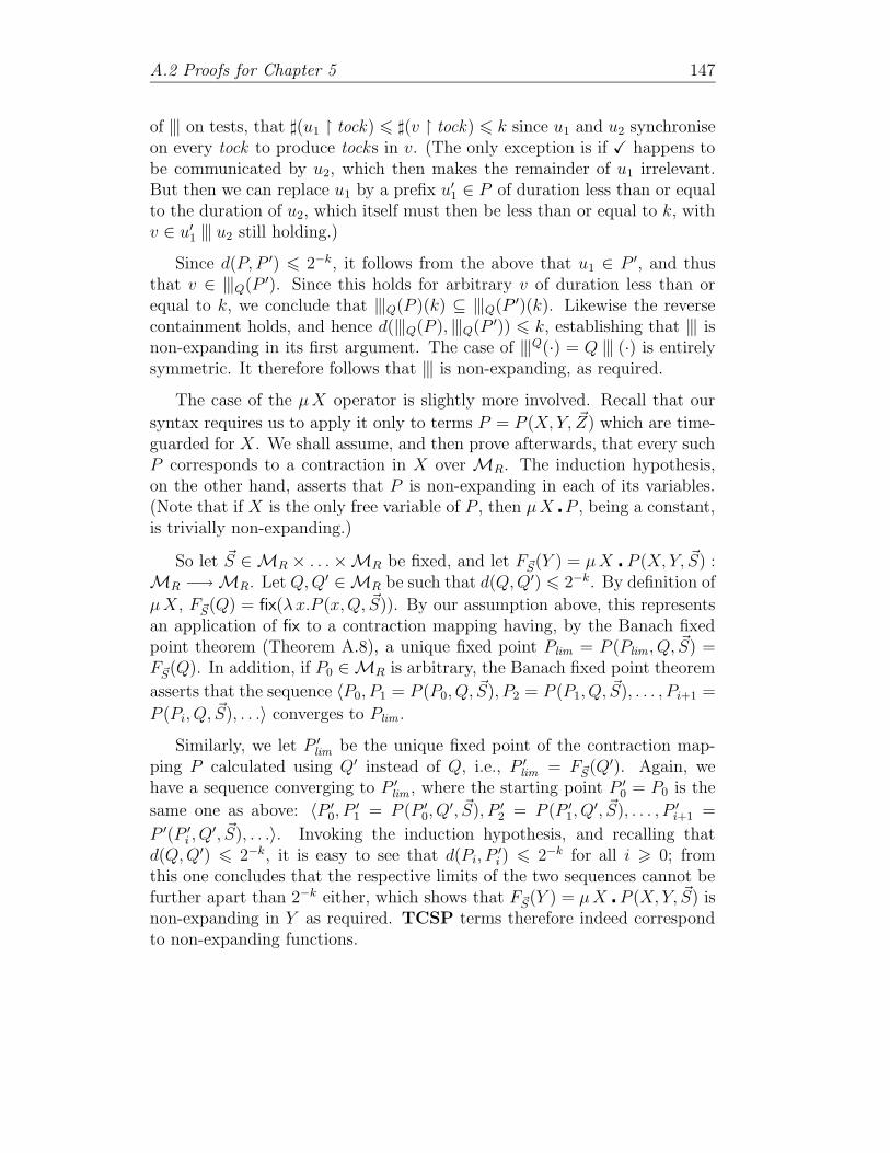
A.2 Proofs for Chapter 5 147
of 9 on tests, that ](u1 � tock) 6 ](v � tock) 6 k since u1 and u2 synchroniseon every tock to produce tocks in v. (The only exception is if X happens tobe communicated by u2, which then makes the remainder of u1 irrelevant.But then we can replace u1 by a prefix u′
1 ∈ P of duration less than or equalto the duration of u2, which itself must then be less than or equal to k, withv ∈ u′
1 9 u2 still holding.)
Since d(P, P ′) 6 2−k, it follows from the above that u1 ∈ P ′, and thusthat v ∈ 9Q(P ′). Since this holds for arbitrary v of duration less than orequal to k, we conclude that 9Q(P )(k) ⊆ 9Q(P ′)(k). Likewise the reversecontainment holds, and hence d(9Q(P ),9Q(P ′)) 6 k, establishing that 9 isnon-expanding in its first argument. The case of 9Q(·) = Q 9 (·) is entirelysymmetric. It therefore follows that 9 is non-expanding, as required.
The case of the µX operator is slightly more involved. Recall that our
syntax requires us to apply it only to terms P = P (X,Y, ~Z) which are time-guarded for X. We shall assume, and then prove afterwards, that every suchP corresponds to a contraction in X over MR. The induction hypothesis,on the other hand, asserts that P is non-expanding in each of its variables.(Note that if X is the only free variable of P , then µX �P , being a constant,is trivially non-expanding.)
So let ~S ∈ MR × . . . ×MR be fixed, and let F~S(Y ) = µX � P (X,Y, ~S) :MR −→ MR. Let Q,Q′ ∈ MR be such that d(Q,Q′) 6 2−k. By definition of
µX, F~S(Q) = fix(λx.P (x,Q, ~S)). By our assumption above, this representsan application of fix to a contraction mapping having, by the Banach fixedpoint theorem (Theorem A.8), a unique fixed point Plim = P (Plim , Q, ~S) =F~S(Q). In addition, if P0 ∈ MR is arbitrary, the Banach fixed point theorem
asserts that the sequence 〈P0, P1 = P (P0, Q, ~S), P2 = P (P1, Q, ~S), . . . , Pi+1 =
P (Pi, Q, ~S), . . .〉 converges to Plim .
Similarly, we let P ′lim
be the unique fixed point of the contraction map-ping P calculated using Q′ instead of Q, i.e., P ′
lim= F~S(Q′). Again, we
have a sequence converging to P ′lim
, where the starting point P ′0 = P0 is the
same one as above: 〈P ′0, P
′1 = P (P ′
0, Q′, ~S), P ′
2 = P (P ′1, Q
′, ~S), . . . , P ′i+1 =
P ′(P ′i , Q
′, ~S), . . .〉. Invoking the induction hypothesis, and recalling thatd(Q,Q′) 6 2−k, it is easy to see that d(Pi, P
′i ) 6 2−k for all i > 0; from
this one concludes that the respective limits of the two sequences cannot befurther apart than 2−k either, which shows that F~S(Y ) = µX � P (X,Y, ~S) isnon-expanding in Y as required. TCSP terms therefore indeed correspondto non-expanding functions.

A.2 Proofs for Chapter 5 148
We now establish the second part of the lemma, namely the assertionthat, if P is time-guarded for X, then P is a contraction in X. (Here thevariable X is arbitrary, but fixed.) We will prove this result by means ofa double induction, as follows. Our first induction will be on the numberof µZ operators appearing in P , for any Z ∈ VAR. Within each suchstep, we will carry out a structural induction over the recursive definitionof time-guardedness (Definition 2.2). Our precise inductive statement is:‘If P contains k recursion operators and P is time-guarded for X, then Prepresents a contraction in X’. We aim to show that, for each k > 0, thisstatement is in fact true of terms which are time-guarded in X. This secondpart is accomplished via the structural induction.
The base case k = 0 corresponds to terms P which are recursion-free:
• Clearly, STOP , SKIP , and WAIT n are contractions in X as they donot have X as a free variable. The case µX � P is vacuously true as itcontains one (rather than zero) recursion operator.
• If Y 6= X, then Y is a contraction in X, again because X does notappear as a free variable in it.
• Assume that the induction hypothesis holds for P , and suppose that theantecedent holds (i.e., P contains no recursion operators and is time-guarded for X), otherwise the result follows vacuously. Then a −→ P ,P \ A, f−1(P ), and f(P ) are clearly contractions in X, since, as shownearlier, the relevant operators are all non-expanding—note that thisresult was obtained independently of any assumption about recursion—and since, as per lemma 5.5, the composition of a contraction and anon-expanding function produces a contraction.
The case µY � P is vacuously true as the term contains a recursionoperator.
• The conclusion also follows in the cases of timeout, external and inter-nal choice, parallel and sequential composition, and interleaving, sincethose operators were all independently shown to be non-expanding.
• Lastly, assume that the induction hypothesis holds for P , and that P istime-guarded for X and time-active. Assume furthermore that neitherP nor Q contains a recursion operator (otherwise the result is vacuouslytrue). We want to conclude that P ; Q is a contraction in X.
Since Q is a term not containing a recursion operator, we can invoke thefirst part of this lemma to conclude that it represents a non-expanding

A.2 Proofs for Chapter 5 149
function, as that part, once again, is easily seen to have been establishedindependently of any assumption about recursion. The induction hy-pothesis and our assumption that P is time-guarded for X imply thatP is a contraction in X. Let us write P = P (X) and Q = Q(X),ignoring for simplicity any other free variable (which at any rate wouldbe considered fixed). One can then prove by a simple structural in-duction over the recursive definition of time-activity that behaviours ofduration j in R ∈ MR give rise to behaviours of duration at least j +1in P (R) ; Q(R): it suffices to show that behaviours of P (R) ; Q(R)consist of behaviours of P (R) of duration at least 1, followed by be-haviours of Q(R), and then recall that P is a contraction and that Qis non-expanding. One then concludes that P ; Q must be a contrac-tion mapping in X with contraction factor at most 1/2. We omit thedetails.
This concludes the base case.
The induction step proceeds in a nearly identical manner, except thatwe can now assume that time-guarded terms containing k or fewer recursionoperators correspond to contraction mappings. We can then repeat the sortof reasoning involving the Banach fixed point theorem which we carried outearlier to discharge our proof obligations. As an illustration, let us show howto handle the case µY � P in the recursive definition of time-guardedness inX.
Our induction hypothesis states that, whenever P ′ is time-guarded in Xand contains k or fewer recursion operators, then P ′ represents a contractionin X. We now assume that the term µY �P contains k+1 recursion operatorsand that P is time-guarded in X; we must show that µY � P corresponds toa contraction in X.
Observe that P = P (Y,X, ~Z) must contain exactly k recursion operators.Since it is time-guarded in X, we can apply the induction hypothesis andconclude that P is a contraction in X. Moreover, P must be time-guarded inY since our syntactic rules only allow an application of the operator µY to
such terms. Make a change of free variables in order to rewrite P (Y,X, ~Z) as
P ′(X,W, ~Z), where W ∈ VAR is a fresh variable. As P was time-guarded inY , P ′ is time-guarded in X, and clearly contains k recursion operator. Ap-plying the induction hypothesis again, we conclude that P ′ corresponds to acontraction in X, and therefore that P is a contraction in Y . Calculating thefixed point by successive iterations, as we did earlier, enables us to concludethat µY � P is non-expanding. And since P is a contraction in X, the same

A.2 Proofs for Chapter 5 150
iteration technique easily yields that µY �P is also a contraction in X, whichis what we were required to show.
This completes the induction step and the proof of the lemma. �
Proposition A.10 (5.7) Let P = P (X, ~Y ) be a TCSP term which is time-
guarded for X. Then µX � P is the unique function F = F (~Y ) such that
F (~Y ) = P (F (~Y ), ~Y ).
Proof This follows immediately from the previous lemma and the Banachfixed point theorem. If G = G(~Y ) is any other function that is a fixed point
of P when substituted for X, we find that, whenever we fix ~Y = ~S, we musthave F (~S) = G(~S) by the uniqueness part of the Banach fixed point theoremand the fact that P~S(X) : MR −→ MR is a contraction. Therefore F = Gas claimed. �
Proposition A.11 (5.13) Finite variability—a program P ∈ TCSP can-not perform unboundedly many actions within a finite number of tocks:
∀ k > 0 � ∃n = n(P, k) � ∀ tr ∈ (ΣXtock
∪ {τ})?�
(Ptr
=⇒ ∧ ](tr � tock) 6 k) ⇒ ]tr 6 n.
We first require a number of preliminaries, definitions and lemmas alike.
The notion of syntactic binding which we will use is quite similar to thatintroduced in the previous section: it consists in functions η : VAR −→TCSP. Note however that, since well-timedness is here a crucial property,we cannot merely constrain the range of our bindings to NODER.
We have standard applications of bindings to terms, substitutions, etc.
We now define the notion of time-bisimulation, an analogue to indexedbisimulations which keeps tracks of time elapsed (number of tocks communi-cated), rather than number of transitions and evolutions witnessed. Since ourtreatment is in many respects similar to that of indexed bisimulations, ourexposition will be terser; omitted proofs, for instance, should be understoodto proceed here more or less as they did earlier.
Let {Rk | k ∈ N} be a family of relations between programs. This set isa time-bisimulation if, for any k > 1, any P, P ′, Q,Q′′ ∈ TCSP, and anyµ ∈ ΣX ∪ {τ}, the following four conditions are met:

A.2 Proofs for Chapter 5 151
(P Rk Q ∧ Ptock−→ P ′) ⇒ ∃Q′ �Q
tock−→ Q′ ∧ P ′ Rk−1 Q′
(P Rk Q ∧ Pµ
−→ P ′) ⇒ ∃Q′ �Qµ
−→ Q′ ∧ P ′ Rk Q′
(P Rk Q ∧ Qtock−→ Q′′) ⇒ ∃P ′′ � P
tock−→ P ′′ ∧ P ′′ Rk−1 Q′′
(P Rk Q ∧ Qµ
−→ Q′′) ⇒ ∃P ′′ � Pµ
−→ P ′′ ∧ P ′′ Rk Q′′.
Given a time-bisimulation {Rk} and two terms P and Q, we formallywrite P Rk Q if, for any syntactic binding η, Pη Rk Qη.
We define a family {∼k | k ∈ N} as follows: for any i > 0,
∼i =⋃
{R | ∃ {Sk | k ∈ N} a time-bisimulation � R = Si}.
We now have:
Lemma A.12
1. {∼k} is a time-bisimulation, the strongest such.
2. Each ∼k is an equivalence relation.
3. Any nodes P and P ′ are ∼0-related.
4. For any k, k′ > 0, if k 6 k′ then ∼k′
⊆ ∼k.
Lemma A.13 For any k > 0, ∼k is preserved by all Timed CSP operatorsother than recursion—in other words, ∼k is a congruence with respect tothese operators.1
We omit the straightforward proof, which proceeds in a manner verysimilar to that of Proposition A.4.
Let {Rk | k ∈ N} be a family of relations between nodes and, for any
k, write Rk to denote the composition ∼k ◦ Rk ◦ ∼k. The set {Rk} is atime-bisimulation up to ∼ if, for any k > 1, any P, P ′, Q,Q′′ ∈ TCSP, andany µ ∈ ΣX ∪ {τ}, the following four conditions are met:
1In fact, it is possible to show that, as with indexed bisimulations, each ∼k is a con-gruence with respect to all of the operators of Timed CSP, but we will not require thismore complicated result here. A proof is given in [Oua00].

A.2 Proofs for Chapter 5 152
(P Rk Q ∧ Ptock−→ P ′) ⇒ ∃Q′ �Q
tock−→ Q′ ∧ P ′ Rk−1 Q′
(P Rk Q ∧ Pµ
−→ P ′) ⇒ ∃Q′ �Qµ
−→ Q′ ∧ P ′ Rk Q′
(P Rk Q ∧ Qtock−→ Q′′) ⇒ ∃P ′′ � P
tock−→ P ′′ ∧ P ′′ Rk−1 Q′′
(P Rk Q ∧ Qµ
−→ Q′′) ⇒ ∃P ′′ � Pµ
−→ P ′′ ∧ P ′′ Rk Q′′.
Lemma A.14 If {Rk |k ∈ N} is a time-bisimulation up to ∼, then, for eachk > 0, Rk ⊆ ∼k.
Proof (Sketch.) One first shows that {Rk} is a full-fledged time-bisimula-tion. This is a straightforward diagram chase requiring only the transitivityof each ∼k (as per Lemma A.12).
Next, one notices that, for any k, Rk ⊆ Rk, since each ∼k is reflexive(Lemma A.12 again).
The result then follows by combining both these observations and invok-ing the maximality of {∼k}. �
If η and η′ are syntactic bindings and k > 0, we write η ∼k η′ if, for allX ∈ VAR, η(X) ∼k η′(X). We then have:
Lemma A.15 Let P ∈ TCSP and η ∼k η′ for some syntactic bindings η,η′, and some fixed k > 0. Then Pη ∼k Pη′.
Proof (Sketch.) Define a family of relations {≈n} as follows. For n 6 k,let ≈n = ≈k = {(Rη,Rη′) |R ∈ TCSP}. For greater values of n, let ≈n = ∅.
We need only show that {≈n} is a time-bisimulation up to ∼. The resultwill follow by taking R = P and invoking Lemma A.14.
We proceed by structural induction on R. Let us tackle the cases of tock -transitions on external choice, along with recursion, in illustration; all othercases are at least as easy.
Without loss of generality, we pick n = k > 1 and thus consider therelation ≈k. Let R = R1 2 R2. Our structural induction hypothesis statesthat (R1η,R1η
′) and (R2η,R2η′) both fulfill the four conditions for {≈k} to be
a time-bisimulation up to ∼. We must show the same holds for (Rη,Rη ′). Asstated above, we shall limit ourselves to (half of) the case of tock -transitions.

A.2 Proofs for Chapter 5 153
So suppose that Rηtock−→ Q. Consulting the relevant inference rules, we
find that we must have R1ηtock−→ Q1, R2η
tock−→ Q2, and Q ≡ Q1 2 Q2.
By the induction hypothesis, we then conclude that R1η′ tock−→ Q′
1, with
Q1 ≈k−1
Q′1, i.e., Q1 ∼
k−1 S1 ≈k−1 S ′
1 ∼k−1 Q′
1.
Since S1 ≈k−1 S ′
1, there is by definition some term E1 such that S1 ≡ E1ηand S ′
1 ≡ E1η′.
Likewise, we find R2η′ tock−→ Q′
2, with Q2 ∼k−1 S2 ≡ E2η ≈k−1 E2η′ ≡
S ′2 ∼
k−1 Q′2.
Let Q′ ≡ Q′1 2 Q′
2. We clearly have Rη′ tock−→ Q′. Moreover, since
∼k−1 preserves the external choice operator (as per Lemma A.13), we have(Q1 2 Q2) ∼
k−1 (S1 2 S2), and likewise for the primed expression.
Stringing everything together, we get
Q ≡ (Q1 2 Q2) ∼k−1 (S1 2 S2) ≡ (E1η 2 E2η) ≡ (E1 2 E2)η
≈k−1
(E1 2 E2)η′ ≡ (E1η
′2 E2η
′) ≡ (S ′1 2 S ′
2) ∼k−1 (Q′
1 2 Q′2) ≡ Q′
i.e., Q ≈k−1
Q′, as required.
We now consider the case of recursion. Note that (µX �R)ητ
−→ (R[µX �R/X])η and likewise (µX � R)η′ τ
−→ (R[µX � R/X])η′ (and these are theonly allowable behaviours). But (R[µX � R/X])η ≈k (R[µX � R/X])η′ bydefinition, so we are done. �
Lemma A.16 If P is a TCSP term which is time-guarded for X, and ηis a syntactic binding, then for any programs Q and Q′, and any k > 0, ifQ ∼k Q′, then P [Q/X]η ∼k+1 P [Q′/X]η.
Proof This is a done by structural induction on the definition of time-guardedness. All cases are straightforward save for the last one, which wetackle here.
We must show that the result holds for P ≡ P1 ; P2 if it holds for P1 andP2. Here P1 is time-guarded for X and time-active, whereas no assumptionsare made about P2.
We are assuming that Q ∼k Q′. From the induction hypothesis, we getthat P1[Q/X]η ∼k+1 P1[Q
′/X]η. Moreover, since P1 is time-active, so are
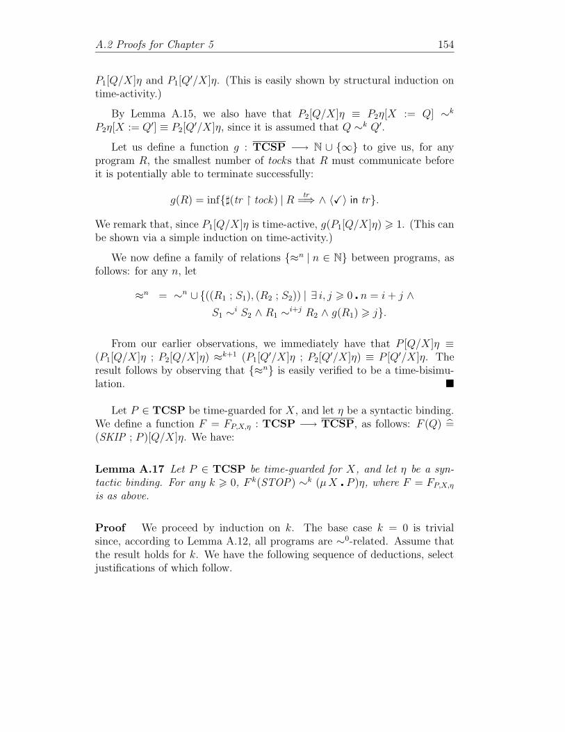
A.2 Proofs for Chapter 5 154
P1[Q/X]η and P1[Q′/X]η. (This is easily shown by structural induction on
time-activity.)
By Lemma A.15, we also have that P2[Q/X]η ≡ P2η[X := Q] ∼k
P2η[X := Q′] ≡ P2[Q′/X]η, since it is assumed that Q ∼k Q′.
Let us define a function g : TCSP −→ N ∪ {∞} to give us, for anyprogram R, the smallest number of tocks that R must communicate beforeit is potentially able to terminate successfully:
g(R) = inf{](tr � tock) | Rtr
=⇒ ∧ 〈X〉 in tr}.
We remark that, since P1[Q/X]η is time-active, g(P1[Q/X]η) > 1. (This canbe shown via a simple induction on time-activity.)
We now define a family of relations {≈n | n ∈ N} between programs, asfollows: for any n, let
≈n = ∼n ∪{((R1 ; S1), (R2 ; S2)) | ∃ i, j > 0 � n = i + j ∧
S1 ∼i S2 ∧ R1 ∼
i+j R2 ∧ g(R1) > j}.
From our earlier observations, we immediately have that P [Q/X]η ≡(P1[Q/X]η ; P2[Q/X]η) ≈k+1 (P1[Q
′/X]η ; P2[Q′/X]η) ≡ P [Q′/X]η. The
result follows by observing that {≈n} is easily verified to be a time-bisimu-lation. �
Let P ∈ TCSP be time-guarded for X, and let η be a syntactic binding.We define a function F = FP,X,η : TCSP −→ TCSP, as follows: F (Q) =(SKIP ; P )[Q/X]η. We have:
Lemma A.17 Let P ∈ TCSP be time-guarded for X, and let η be a syn-tactic binding. For any k > 0, F k(STOP) ∼k (µX � P )η, where F = FP,X,η
is as above.
Proof We proceed by induction on k. The base case k = 0 is trivialsince, according to Lemma A.12, all programs are ∼0-related. Assume thatthe result holds for k. We have the following sequence of deductions, selectjustifications of which follow.

A.2 Proofs for Chapter 5 155
F k+1(STOP) ≡ F (F k(STOP))
≡ (SKIP ; P )[F k(STOP)/X]η
≡ SKIP ; (P [F k(STOP)/X]η)
∼k+1 SKIP ; (P [(µX � P )η/X]η) (1)
∼k+1 (µX � P )η. (2)
This concludes the induction step. (1) follows from Lemma A.16, using thefact that F k(STOP) ∼k (µX � P )η by the induction hypothesis, and thefact that left sequential composition with SKIP preserves time-bisimulation(thanks to Lemma A.13). (2) rests on the observation that SKIP ; (P [(µX �P )η/X]η) ∼n (µX � P )η for any n > 0, as an immediate calculation of thepossible executions will attest. �
Lemma A.18 Let P, P ′ ∈ TCSP, k > 1, and suppose that P ∼k P ′. Then
for any τ -trace tr with ](tr � tock) < k and such that Ptr
=⇒, we have P ′ tr=⇒.
Proof The τ -trace tr must originate from some execution e ∈ execR(P ).Since P ∼k P ′, this execution can be matched for a duration of k tocks bysome execution e′ ∈ execR(P ′). It is plain that e′ also gives rise to tr . �
We are now in a position to give the proof of Proposition A.11.
Proof (Sketch.) We proceed by structural induction on terms. Specifi-cally, let us call a program finitely variable if it satisfies the conclusion ofProposition A.11. We show by induction on P that whenever η is a syntac-tic binding such that η(X) is finitely variable for all X ∈ VAR, then Pη isfinitely variable. Here P ∈ TCSP, and in particular is well-timed.
All cases of the structural induction are straightforward save for recursion,which we handle below.
We are assuming that Pη is finitely variable whenever η is pointwisefinitely variable, and aim to show that (µX � P )η is also finitely variablewhenever η is pointwise finitely variable. Note that our grammar requires Pto be time-guarded for X.
Let k > 0 be given, and let η be fixed. By Lemma A.16, (µX �P )η ∼k+1
F k+1(STOP), where F = FP,X,η is the function satisfying F (Q) = (SKIP ;P )[Q/X]η defined earlier.
We first show that F n(STOP) is finitely variable for all n > 0. This is asimple induction on n which has a trivial base case n = 0. For the induction

A.2 Proofs for Chapter 5 156
step, assuming the statement holds for n, we have
F n+1(STOP) ≡ F (F n(STOP))
≡ (SKIP ; P )[F n(STOP)/X]η
≡ SKIP ; (P (η[X := F n(STOP)])).
Now P (η[X := F n(STOP)]) is finitely variable by the structural inductionhypothesis on P , our assumptions on η, and the induction hypothesis onn. Therefore SKIP ; (P (η[X := F n(STOP)])) ≡ F n+1(STOP) are finitelyvariable as well, which completes the induction on n.
Let us now consider any τ -trace tr with ](tr � tock) 6 k and such
that (µX � P )ηtr
=⇒. Since (µX � P )η ∼k+1 F k+1(STOP), we can invoke
Lemma A.18 to conclude that F k+1(STOP)tr
=⇒. But since F k+1(STOP) isfinitely variable, we must have ]tr 6 n, for some uniform n = n(k). Sincetr was an arbitrary τ -trace of (µX � P )η containing k tocks or fewer, weconclude that (µX � P )η is indeed finitely variable, as required. �
Theorem A.19 (5.14) For any TCSP program P , we have
ΦR(P ) = RJP K.
Proof We first need some preliminaries. Define a syntactic binding tobe a function η : VAR −→ TCSP. Syntactic bindings are the operationalanalogue of semantic bindings.
For P ∈ TCSP, the application Pη ∈ TCSP is obtained via substitutionof programs for free variables in the obvious way.
Given a syntactic binding η, define the associated semantic binding η asfollows: for any X ∈ VAR, η(X) = ΦR(η(X)). (See, however, the caveatbelow.)
The more general statement we would then like to prove is that, for anyP ∈ TCSP, and any syntactic binding η,
ΦR(Pη) = RJP Kη. (A.1)
It is plain that this would establish the theorem, since programs have no freevariables and therefore make bindings irrelevant.
The problem with this approach is that, in spite of our claim two para-graphs ago, there is no a priori guarantee that η is indeed a semantic binding,
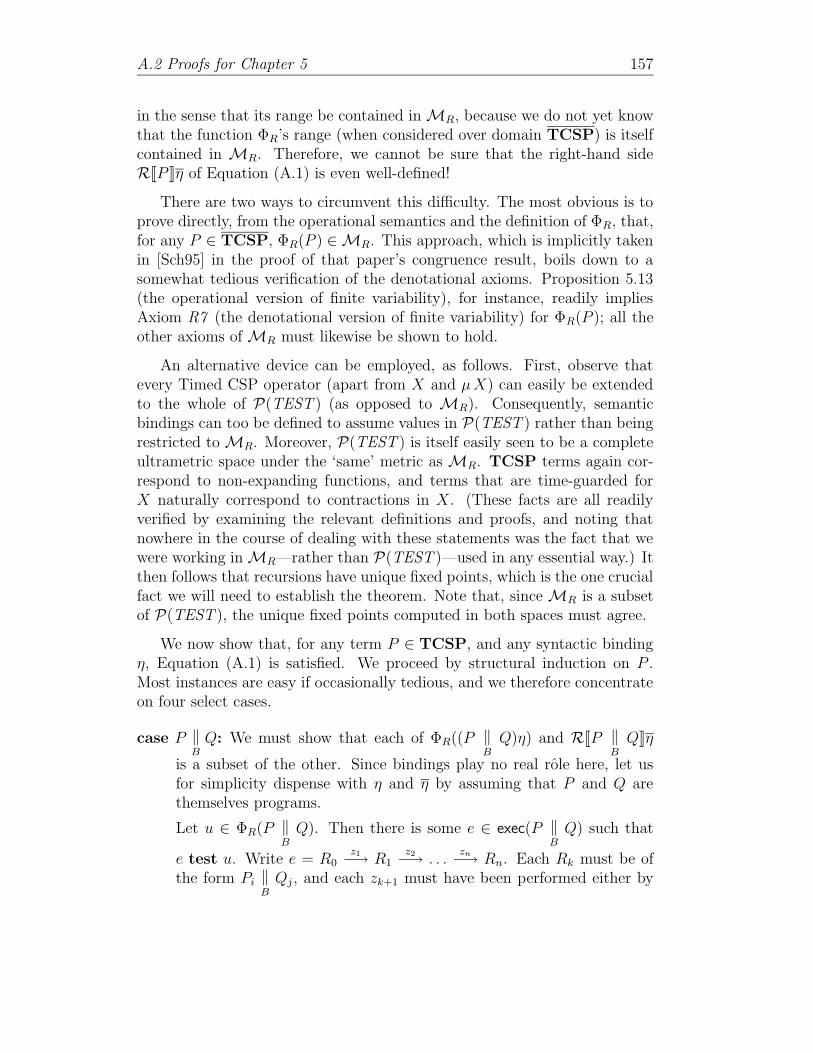
A.2 Proofs for Chapter 5 157
in the sense that its range be contained in MR, because we do not yet knowthat the function ΦR’s range (when considered over domain TCSP) is itselfcontained in MR. Therefore, we cannot be sure that the right-hand sideRJP Kη of Equation (A.1) is even well-defined!
There are two ways to circumvent this difficulty. The most obvious is toprove directly, from the operational semantics and the definition of ΦR, that,for any P ∈ TCSP, ΦR(P ) ∈ MR. This approach, which is implicitly takenin [Sch95] in the proof of that paper’s congruence result, boils down to asomewhat tedious verification of the denotational axioms. Proposition 5.13(the operational version of finite variability), for instance, readily impliesAxiom R7 (the denotational version of finite variability) for ΦR(P ); all theother axioms of MR must likewise be shown to hold.
An alternative device can be employed, as follows. First, observe thatevery Timed CSP operator (apart from X and µX) can easily be extendedto the whole of P(TEST ) (as opposed to MR). Consequently, semanticbindings can too be defined to assume values in P(TEST ) rather than beingrestricted to MR. Moreover, P(TEST ) is itself easily seen to be a completeultrametric space under the ‘same’ metric as MR. TCSP terms again cor-respond to non-expanding functions, and terms that are time-guarded forX naturally correspond to contractions in X. (These facts are all readilyverified by examining the relevant definitions and proofs, and noting thatnowhere in the course of dealing with these statements was the fact that wewere working in MR—rather than P(TEST )—used in any essential way.) Itthen follows that recursions have unique fixed points, which is the one crucialfact we will need to establish the theorem. Note that, since MR is a subsetof P(TEST ), the unique fixed points computed in both spaces must agree.
We now show that, for any term P ∈ TCSP, and any syntactic bindingη, Equation (A.1) is satisfied. We proceed by structural induction on P .Most instances are easy if occasionally tedious, and we therefore concentrateon four select cases.
case P ‖B
Q: We must show that each of ΦR((P ‖B
Q)η) and RJP ‖B
QKη
is a subset of the other. Since bindings play no real role here, let usfor simplicity dispense with η and η by assuming that P and Q arethemselves programs.
Let u ∈ ΦR(P ‖B
Q). Then there is some e ∈ exec(P ‖B
Q) such that
e test u. Write e = R0z1−→ R1
z2−→ . . .zn−→ Rn. Each Rk must be of
the form Pi ‖B
Qj, and each zk+1 must have been performed either by

A.2 Proofs for Chapter 5 158
both of Pi and Qj (precisely when zk+1 ∈ B ∪ {tock}) or by exactlyone of Pi and Qj.
We can thus decompose the execution e into executions eP = P0x1−→
P1x2−→ . . .
xl−→ Pl ∈ exec(P ) and eQ = Q0y1−→ Q1
y2−→ . . .
ym−→ Qm ∈
exec(Q). Write eP test uP and eQ test uQ, where uP and uQ aremaximal such tests under the information ordering ≺; that is to say,the refusals in these tests are as large as possible.
We now claim that u ∈ uP ‖B
uQ. This is a simple inspection of the
definitions. Consider, for instance, Rk
zk+1−→ Rk+1, where Rk = Pi ‖
B
Qj.
If zk+1 = τ , then this particular transition of e contributes nothingto u, and can be dismissed. Note that the corresponding xi+1 or yj+1
will itself also be a τ and contribute nothing to uP or uQ. Let ustherefore first suppose that zk+1 ∈ B ∪ {tock}. If D is a refusal suchthat Rk test 〈D〉, it easily follows from the fact that Rk ≡ Pi ‖
B
Qj
that there are (maximal) refusals A and C such that Pi test 〈A〉 andQj test 〈C〉 and 〈D〉 ∈ 〈A〉 ‖
B
〈C〉. And since zk+1 ∈ B ∪ {tock}, we
must have xi+1 = yj+1 = zk+1 and Rk+1 ≡ Pi+1 ‖B
Qj+1. We therefore
see that the contribution 〈D, zk+1〉 of e in u is accounted for by thecontributions 〈A, zk+1〉 and 〈C, zk+1〉, respectively of eP and eQ to uP
and uQ.
A similar argument handles the case zk+1 /∈ B ∪ {tock , τ}. We con-clude that indeed u ∈ uP ‖
B
uQ. Since eP ∈ exec(P ) and eP test uP , we
have, by definition, that uP ∈ ΦR(P ). We can then invoke the induc-tion hypothesis to conclude that uP ∈ RJP K. Likewise, uQ ∈ RJQK.Naturally, it follows by definition that u ∈ RJP ‖
B
QK, as required.
To establish the reverse containment, one starts with u ∈ RJP ‖B
QK
and then essentially retraces one’s steps back into the statement thatu ∈ ΦR(P ‖
B
Q). This simple procedure requires little else than careful
bookkeeping, and is left to the reader.
case P \ A: Here again let us disregard syntactic and semantic bindingswhich are at any rate of little importance. Let v ∈ ΦR(P \ A). Wemust then have e = P0 \ A
x1−→ P1 \ Ax2−→ . . .
xn−→ Pn \ A ∈exec(P \ A) such that e test v. It is an easy matter to show that
the execution e ‘originates’ from some execution e′ = P0y1−→ P1
y2−→
A.2 Proofs for Chapter 5 159
. . .yn−→ Pn ∈ exec(P ), where xi = yi if yi /∈ A, and otherwise xi = τ ,
for all 1 6 i 6 n. Note, in addition, that, thanks to Rule 5.28 and
Proposition 5.10, whenever Pitock−→ Pi+1, it must have been the case
that initτ (Pi) ∩ (A ∪ {τ}) = ∅.
Let u be a ≺-maximal test with the property that e′ test u. Note that,by the property of e′ quoted above, it must be the case that u is A-urgent. And since u ∈ ΦR(P ), we can invoke the induction hypothesisto conclude that u ∈ RJP K. It remains to show that v ≺ u \ A. Butthis easily follows from the definition of hiding on tests together withthe definition of the relation test.
The reverse containment is easily obtained by reversing the argumentjust given.
case X: We have that ΦR(Xη) = ΦR(η(X)) = η(X) = RJXKη as required.
case µX � P : We recall our induction hypothesis which states that, if ρ isany syntactic binding, then ΦR(Pρ) = RJP Kρ. We now have
ΦR((µX � P )η) = ΦR(P [µX � P/X]η) (1)
= ΦR(P (η[X := (µX � P )η])) (2)
= RJP Kη[X := (µX � P )η] (3)
= RJP K(η[X := ΦR((µX � P )η)]). (4)
To see (1), notice first that the only initial operational step allowed(µX �P )η is a τ -transition into P [µ X �P/X]η. Since the test relationdiscards τ -transitions from executions, (1) follows. (2) is an immediateconsequence of the fact that P [µ X � P/X]η ≡ P (η[X := (µX � P )η]).(3) is an application of the induction hypothesis, and (4) follows fromthe fact that η[X := (µX � P )η](Y ) is by definition equal to ΦR(η[X :=(µX � P )η](Y )), which is ΦR((µX � P )η) if Y ≡ X, and ΦR(η(Y )) =η(Y ) otherwise.
This string of equalities implies that ΦR((µX � P )η) is a fixed point ofthe function λx.RJP K(η[X := x]) : P(TEST ) −→ P(TEST ). Sincewe know that RJµX � P Kη is the unique fixed point of this function,we must conclude that ΦR((µX � P )η) = RJµX � P Kη as required.
�

Appendix B
Power-Simulations and ModelChecking
We define a power-simulation relation on the labelled transition systems ofprograms and show that it corresponds precisely to test refinement in MR.This provides us with a model checking algorithm for deciding refinementof processes with finite LTS’s. The ideas presented here are, in much lesssophisticated form, similar to those upon which FDR refinement checks arebased—more on this topic can be found in [Ros97].
Let P ∈ NODER be fixed. For u ∈ TEST , let P/u represent the set ofnodes reachable from P upon observing the test u_〈•〉 (the last refusal of ubeing discarded). Formally:
P/u = {Q ∈ NODER | ∃ e_Q ∈ execR(P ) � e_Q test u_〈•〉}.
We use this to build the power labelled transition system PLTSR(P ) of P ,as follows. Its set of power nodes is PLTSN
R = {P/u | u ∈ TEST}, with anoriented edge (A, a)—where A ∈ REF and a ∈ ΣX
tock—from P/u to P/v if
P/(u_〈A, a, •〉) = P/v; we represent this with the notation P/uA,a−→ P/v.
We remark that PLTSR(P ) is finite whenever LTSR(P ) is. Note moreoverthat PLTSR(P ) is always deterministic: no power node ever has two distinctidentically labelled edges emerging from it.
Given a power node p ∈ PLTSNR (P ), we let refs(p) = {A ∈ REF | ∃Q ∈
p �Q ref A}.
Let P,Q ∈ NODER. We say that a relation R on PLTSNR (P )×PLTSN
R (Q)is a power-simulation if the following condition holds:

B Power-Simulations and Model Checking 161
∀ q ∈ PLTSNR (Q) � ∀ p ∈ PLTSN
R (P ) � p R q ⇒
(refs(q) ⊆ refs(p) ∧
∀(qe
−→ q′) ∈ PLTSR(Q)�
∃ p′ � pe
−→ p′ ∈ PLTSR(P ) ∧ p′ R q′).
We now have:
Definition B.1 For P,Q ∈ NODER, we say that P power-simulates Q,written P psimR Q, if there exists R a power-simulation on PLTSN
R (P ) ×PLTSN
R (Q) such that P/〈〉 R Q/〈〉.
Finally, we have the following main result:
Theorem B.1 For any P,Q ∈ TCSP,
P psimR Q ⇔ P vR Q.
Proof (Sketch.) Follows easily from Theorem 5.14 and the definition ofpower-simulation. �
Theorem B.1 yields an algorithm to decide the refinement P vR Q when-ever the labelled transition systems of P and Q are finite. Consider the finiteset PLTSN
R (P ) × PLTSNR (Q), and let Check and Pend be two ‘set-variables’,
both intended as subsets of PLTSNR (P ) × PLTSN
R (Q), with Check initiallyempty and Pend initially containing the single pair (P/〈〉, Q/〈〉). Repeat thefollowing steps until Pend is empty:
1. Pick a pair (p, q) ∈ Pend.
2. Check whether refs(q) ⊆ refs(p). If this is not the case, exit immediatelywith the answer P v6 R Q.
3. For each edge qe
−→ q′ in PLTSR(Q), check whether there is an edgep
e−→ p′ in PLTSR(P ). If this is not the case, exit immediately with
the answer P v6 R Q.
4. Add (p, q) to Check.
5. For each edge qe
−→ q′ in PLTSR(Q) and corresponding unique edgep
e−→ p′ in PLTSR(P ), add (p′, q′) to Pend unless (p′, q′) is in Check.

B Power-Simulations and Model Checking 162
It is not difficult to see that this algorithm will always terminate. If theloop is successfully exited (i.e., upon finding Pend empty), then Check is apower-simulation and thus P vR Q. On the other hand, if P v6 R Q, thenthe loop will necessarily be exited with this answer at some point. The easyverification of these claims is left to the reader.
We conclude by pointing out that refinement in MUR can be decided,whenever the labelled transition systems of the processes involved are finite,by using similar definitions and a similar algorithm.
Appendix C
Operational Semantics for theTimed Failures-Stability Model
We give an operational semantics for Reed and Roscoe’s timed failures-stability model for Timed CSP, denoted here MTFS , with associated semanticmap FTSJ·K. This model, presented in [RR87, Ree88, RR99], improves uponMTF in that it associates a stability value to every timed failure, which valuerepresents the least time by which a process, given its observed behaviour,can be guaranteed to have become stable. Stability here refers to invarianceunder the passage of time.
To capture this notion operationally, two different types of evolutions areintroduced: stable evolutions (implying that the process has already reachedstability), as well as unstable evolutions (implying that the process is headedtowards some eventual internal transition, and is therefore unstable).
The style and conventions of this appendix are very similar to those ofSection 3.2. We use as nodes the previously defined collection NODETF ofTimed CSP programs with fractional delays and no well-timedness require-ments. Open nodes, likewise, are elements of NODETF . a and b stand for(non-tock) visible events, i.e., belong to ΣX. A ⊆ Σ and B ⊆ ΣX. µ can be a
visible event or a silent one (µ ∈ ΣX ∪ {τ}). Pµ
−→ P ′ means P can performan immediate and instantaneous µ-transition, and become P ′ (communicat-
ing µ in the process if µ is a visible event). Pµ
X−→ means that P cannot
possibly do a µ at that particular time. Pt 1 P ′ implies that P is a stable
node, and can become P ′ (also stable) simply by virtue of letting t units of
time elapse, where t is a non-negative real number. Pt 2 P ′ states that the

C Operational Semantics for the Timed Failures-Stability Model 164
unstable node P can become P ′ by letting t time units elapse. When using
the generic notationt x, it is understood that x stands for either 1 or 2.
The transition rules are as follows:
STOPt 1 STOP
(C.1)
SKIPt 1 SKIP
(C.2)
SKIPX
−→ STOP(C.3)
WAIT ut 2 WAIT (u − t)
[ t 6 u ] (C.4)
WAIT 0τ
−→ SKIP(C.5)
P1t x P ′
1
P1
u� P2
t 2 P ′
1
u−t� P2
[ t 6 u ] (C.6)
P1
0� P2
τ−→ P2
(C.7)
P1τ
−→ P ′1
P1
u� P2
τ−→ P ′
1
u� P2
(C.8)
P1a
−→ P ′1
P1
u� P2
a−→ P ′
1
(C.9)

C Operational Semantics for the Timed Failures-Stability Model 165
(a −→ P )t 1 (a −→ P )
(C.10)
(a −→ P )a
−→ P(C.11)
(a : A −→ P (a))t 1 (a : A −→ P (a))
(C.12)
(a : A −→ P (a))b
−→ P (b)[ b ∈ A ] (C.13)
P1t x P ′
1 P2t y P ′
2
P1 2 P2t max{x,y} P ′
1 2 P ′2
(C.14)
P1τ
−→ P ′1
P1 2 P2τ
−→ P ′1 2 P2
P2τ
−→ P ′2
P1 2 P2τ
−→ P1 2 P ′2
(C.15)
P1a
−→ P ′1
P1 2 P2a
−→ P ′1
P2a
−→ P ′2
P1 2 P2a
−→ P ′2
(C.16)
P1 u P2τ
−→ P1 P1 u P2τ
−→ P2
(C.17)
P1t x P ′
1 P2t y P ′
2
P1 ‖B
P2t max{x,y} P ′
1 ‖B
P ′2
(C.18)
P1µ
−→ P ′1
P1 ‖B
P2µ
−→ P ′1‖B
P2
[ µ /∈ B, µ 6= X ] (C.19a)

C Operational Semantics for the Timed Failures-Stability Model 166
P2µ
−→ P ′2
P1 ‖B
P2µ
−→ P1 ‖B
P ′2
[ µ /∈ B, µ 6= X ] (C.19b)
P1a
−→ P ′1 P2
a−→ P ′
2
P1 ‖B
P2a
−→ P ′1‖B
P ′2
[ a ∈ B ] (C.20)
P1X
−→ P ′1
P1 ‖B
P2X
−→ P ′1
[X /∈ B ]P2
X−→ P ′
2
P1 ‖B
P2X
−→ P ′2
[X /∈ B ] (C.21)
P1t x P ′
1 P2t y P ′
2
P1 9 P2t max{x,y} P ′
1 9 P ′2
(C.22)
P1µ
−→ P ′1
P1 9 P2µ
−→ P ′1 9 P2
[ µ 6= X ] (C.23a)
P2µ
−→ P ′2
P1 9 P2µ
−→ P1 9 P ′2
[ µ 6= X ] (C.23b)
P1X
−→ P ′1
P1 9 P2X
−→ P ′1
P2X
−→ P ′2
P1 9 P2X
−→ P ′2
(C.24)
P1t x P ′
1 P1X
X−→
P1 ; P2t x P ′
1 ; P2
(C.25)
P1X
−→ P ′1
P1 ; P2τ
−→ P2
(C.26)
P1µ
−→ P ′1
P1 ; P2µ
−→ P ′1 ; P2
[ µ 6= X ] (C.27)

C Operational Semantics for the Timed Failures-Stability Model 167
Pt x P ′ ∀ a ∈ A � P
aX−→
P \ At x P ′ \ A
(C.28)
Pa
−→ P ′
P \ Aτ
−→ P ′ \ A[ a ∈ A ] (C.29)
Pµ
−→ P ′
P \ Aµ
−→ P ′ \ A[ µ /∈ A ] (C.30)
Pt x P ′
f−1(P )t x f−1(P ′)
(C.31)
Pµ
−→ P ′
f−1(P )µ
−→ f−1(P ′)[ µ ∈ {τ,X} ] (C.32)
Pf(a)−→ P ′
f−1(P )a
−→ f−1(P ′)(C.33)
Pt x P ′
f(P )t x f(P ′)
(C.34)
Pµ
−→ P ′
f(P )µ
−→ f(P ′)[ µ ∈ {τ,X} ] (C.35)
Pa
−→ P ′
f(P )f(a)−→ f(P ′)
(C.36)
µX � Pτ
−→ P [(µX � P )/X].(C.37)
The remark made in Section 3.2 concerning negative premisses (appearing

C Operational Semantics for the Timed Failures-Stability Model 168
in Rules C.25 and C.28) applies here as well.
We now present, without proof, a number of properties enjoyed by thisoperational semantics.
If P and Q are open nodes, we write P ≡ Q to indicate that P and Qare syntactically identical.
If P is a closed node, we define initTFS (P ) to be the set of visible eventsthat P can immediately perform: initTFS (P ) = {a ∈ ΣX | P
a−→}.
For P a closed node, we define an execution of P to be a sequence e =P0
z17−→ P1z27−→ . . .
zn7−→ Pn (with n > 0), where P0 ≡ P , the Pi’s are nodes,
and each subsequence Pi
zi+17−→ Pi+1 in e is either a transition Pi
µ−→ Pi+1
(with zi+1 = µ), or an evolution Pit x Pi+1 (with zi+1 = t). In addition,
every such transition or evolution must be validly allowed by the operationalinference Rules C.1–C.37. The set of executions of P is written execTFS (P ),or exec(P ) for short. By convention, writing down a transition (or sequencethereof) such as P
a−→ P ′, is equivalent to stating that P
a−→ P ′ ∈ exec(P );
the same, naturally, goes for evolutions.
Every execution e gives rise to a timed τ -trace abs(e) in the obvious way,by removing nodes and evolutions from the execution, but recording events’time of occurrence in agreement with e’s (stable and unstable) evolutions.
The duration dur(e) of an execution e is equal to the sum of its (stableand unstable) evolutions.
Proposition C.1 A node cannot be both stable and unstable:
(Pt x P ′ ∧ P
t′
y P ′′) ⇒ x = y.
Proposition C.2 A stable node is invariant under the passage of time, andcan evolve up to any time:
Pt 1 P ′ ⇔ (P ≡ P ′ ∧ ∀ t′ > 0 � P
t′
1 P ).
Proposition C.3 Time determinacy:
(Pt x P ′ ∧ P
t x P ′′) ⇒ P ′ ≡ P ′′.
Proposition C.4 Persistency—the set of possible initial visible events re-mains constant under evolution:
Pt x P ′ ⇒ init(P ) = init(P ′).

C Operational Semantics for the Timed Failures-Stability Model 169
Proposition C.5 Time continuity:
Pt+t′
x P ′ ⇔ ∃P ′′ � Pt x P ′′ t′
x P ′.
Proposition C.6 Maximal progress, or τ -urgency:
Pτ
−→ ⇒ ∀ t > 0 � @ P ′ � Pt x P ′.
Corollary C.7
(Pt x P ′ τ
−→ ∧ Pt′
x P ′′ τ−→) ⇒ (t = t′ ∧ x = 2).
Proposition C.8 A node P can always evolve up to the time of the next τaction, or up to any time if no τ action lies ahead:
∀ t > 0 � (@ P ′ � Pt x P ′) ⇒ (P
τ−→ ∨ ∃ t′ < t, P ′′ � P
t′
2 P ′′ τ−→).
Proposition C.9 An unstable node cannot evolve forever:
Pt 2 P ′ ⇒ ∃ t′, P ′′ � P
t′
2 P ′′ τ−→.
Proposition C.10 Finite variability—a program P ∈ TCSP cannot per-form unboundedly many action in a finite amount of time:
∀ t > 0 � ∃n = n(P, t) ∈ N � ∀ e ∈ exec(P ) � dur(e) 6 t ⇒ ]abs(e) 6 n.
Unsurprisingly, this operational semantics has tight connections with theother operational semantics presented in this thesis, and in particular withthat associated with MTF :
Proposition C.11 For any program P ∈ TCSP,
Pµ
−→ P ′ ∈ execTF ⇔ Pµ
−→ P ′ ∈ execTFS
Pt P ′ ∈ execTF ⇔ ∃x � P
t x P ′ ∈ execTFS .

C Operational Semantics for the Timed Failures-Stability Model 170
A set of visible events is refused by a node P if P cannot immediatelyperform a τ -transition and has no valid initial transition labelled with anevent from that set. Thus for A ⊆ ΣX, we write P ref A if P
τX−→ ∧
A ∩ init(P ) = ∅.
An execution e of a node P is said to fail a timed failure-stability triple(s, α,ℵ) (where α ∈ R+ represents an approximation from below of the sta-bility value of P on (s,ℵ)) if the timed trace s corresponds to the executione, the nodes of e can always refuse the relevant parts of ℵ, and α is the leasttime following the completion of all transitions in e by which P is not ob-served to be unstable. We write this relation as e failS (s, α,ℵ). It is definedinductively on e as follows:
P failS (〈〉, 0, ∅) ⇔ true
(Pτ
−→)_e′ failS (s, α,ℵ) ⇔ e′ failS (s, α,ℵ)
(Pa
−→)_e′ failS (〈(0, a)〉_s′, α,ℵ) ⇔ a 6= τ ∧ e′ failS (s′, α,ℵ)
(Pt 2)_e′ failS (s, α,ℵ) ⇔ P ref σ(ℵ |� t) ∧
e′ failS (s − t, α − t,ℵ − t)
(Pt 1)_e′ failS (〈〉, 0,ℵ) ⇔ abs(e′) = 〈〉 ∧ P ref σ(ℵ) ∧
end(ℵ) 6 t + dur(e′)
(Pt 1)_e′ failS (s, α,ℵ) ⇔ abs(e′) 6= 〈〉 ∧ P ref σ(ℵ |� t) ∧
e′ failS (s − t, α − t,ℵ − t).
The SUP operator on sets of timed failure-stability triples is taken from[RR99]:
SUP(S) = {(s, α,ℵ) | (s,ℵ) ∈ TFailures(S) ∧ α = sup{β | (s, β,ℵ) ∈ S}}
where TFailures((s, α,ℵ)) = (s,ℵ), etc.
Finally, we define the function ΦTFS , which extracts the timed failure-stability denotational representation of a program from its set of executions.
Definition C.1 For P ∈ TCSP, we set
ΦTFS (P ) = SUP{(s, α,ℵ) | ∃ e ∈ execTFS (P ) � e failS (s, α,ℵ)}.
We can now state the chief congruence result:
Theorem C.12 For any TCSP program P , we have
ΦTFS (P ) = FTSJP K.

Bibliography
[ACD90] R. Alur, C. Courcoubetis, and D. Dill. Model-checking for real-time systems. In Proceedings of the Fifth Annual Symposiumon Logic in Computer Science (LICS 90), pages 414–425. IEEEComputer Society Press, 1990.
[ACD93] R. Alur, C. Courcoubetis, and D. Dill. Model-checking in densereal-time. Information and Computation, 104(1):2–34, 1993.
[ACH94] R. Alur, C. Courcoubetis, and T. Henzinger. The observationalpower of clocks. In Proceedings of the Fifth International Confer-ence on Concurrency Theory (CONCUR 94), volume 836, pages162–177. Springer LNCS, 1994.
[AD94] R. Alur and D. Dill. A theory of timed automata. TheoreticalComputer Science, 126:183–235, 1994.
[AH93] R. Alur and T. A. Henzinger. Real-time logics: Complexityand expressiveness. Information and Computation, 104(1):35–77, 1993.
[AH94] R. Alur and T. A. Henzinger. A really temporal logic. Journalof the ACM, 41(1):181–204, 1994.
[AHR98] R. Alur, T. A. Henzinger, and S. K. Rajamani. Symbolic explo-ration of transition hierarchies. In Proceedings of the FourthWorkshop on Tools and Algorithms for the Construction andAnalysis of Systems (TACAS 98), volume 1384, pages 330–344.Springer LNCS, 1998.
[AK96] R. Alur and R. P. Kurshan. Timing analysis in Cospan. InProceedings of Hybrid Systems III, volume 1066, pages 220–231.Springer LNCS, 1996.

Bibliography 172
[BB91] J. C. M. Baeten and J. A. Bergstra. Real time process algebra.Formal Aspects of Computing, 3:142–188, 1991.
[BCM+92] J. Burch, E. Clarke, K. McMillan, D. Dill, and L. Hwang. Sym-bolic model checking: 1020 states and beyond. Information andComputation, 98(2):142–170, 1992.
[BLL+96] J. Bengtsson, K. G. Larsen, F. Larsen, P. Pettersson, and W. Yi.UppAal: A tool-suite for automatic verification of real-timesystems. In Proceedings of Hybrid Systems III, volume 1066,pages 232–243. Springer LNCS, 1996.
[BLP+99] G. Behrmann, K. Larsen, J. Pearson, C. Weise, and W. Yi.Efficient timed reachability analysis using clock difference di-agrams. In Proceedings of the Eleventh International Confer-ence on Computer-Aided Verification (CAV 99), volume 1633.Springer LNCS, 1999.
[BSV95] F. Balarin and A. L. Sangiovanni-Vincentelli. An iterative ap-proach to verification of real-time systems. Formal Methods inSystem Design, 6:67–95, 1995.
[CG95] R. Chapman and M. Goldsmith. Translating timer automata toTCSP. Formal Systems Design and Development, Inc., 1995.
[Che92] L. Chen. Timed Processes: Models, Axioms and Decidability.PhD thesis, University of Edinburgh, 1992.
[CLM97] R. Cleaveland, G. Luttgen, and M. Mendler. An algebraic the-ory of multiple clocks. In Proceedings of the Eighth Interna-tional Conference on Concurrency Theory (CONCUR 97), vol-ume 1243, pages 166–180. Springer LNCS, 1997.
[Dav91] J. Davies. Specification and Proof in Real-Time Systems. PhDthesis, Oxford University, 1991.
[DOTY96] C. Daws, A. Olivero, S. Tripakis, and S. Yovine. The tool Kro-
nos. In Proceedings of Hybrid Systems III, volume 1066, pages208–219. Springer LNCS, 1996.
[DS95] J. Davies and S. A. Schneider. A brief history of Timed CSP.Theoretical Computer Science, 138(2):243–271, 1995.

Bibliography 173
[Fid93] C. J. Fidge. A formal definition of priority in CSP. ACM Trans-actions on Programming Languages and Systems, 15(4):681–705,1993.
[GB87] R. Gerth and A. Boucher. A timed failures model for extendedcommunicating processes. In Proceedings of the Fourteenth Inter-national Colloquium on Automata, Languages and Programming(ICALP 87), volume 267, pages 95–114. Springer LNCS, 1987.
[Hen96] T. A. Henzinger. The theory of hybrid automata. In Proceed-ings of the Eleventh Annual Symposium on Logic in ComputerScience (LICS 96). IEEE Computer Society Press, 1996.
[Hen98] T. A. Henzinger. It’s about time: Real-time logics reviewed.In Proceedings of the Ninth International Conference on Con-currency Theory (CONCUR 98), volume 1466, pages 439–454.Springer LNCS, 1998.
[HHWT97] T. A. Henzinger, P.-H. Ho, and H. Wong-Toi. HyTech: Amodel checker for hybrid systems. In Proceedings of the NinthInternational Conference on Computer-Aided Verification (CAV97), volume 1254, pages 460–463. Springer LNCS, 1997.
[HJL93] C. L. Heitmeyer, R. D. Jeffords, and B. G. Labaw. A bench-mark for comparing different approaches for specifying and veri-fying real-time systems. In Proceedings of the Tenth InternationalWorkshop on Real-Time Operating Systems and Software, 1993.
[HK97] T. A. Henzinger and O. Kupferman. From quantity to quality.In Proceedings of the First International Workshop on Hybridand Real-time Systems (HART 97), volume 1201, pages 48–62.Springer LNCS, 1997.
[HKV96] T. A. Henzinger, O. Kupferman, and M. Y. Vardi. A space-efficient on-the-fly algorithm for real-time model checking. InProceedings of the Seventh International Conference on Con-currency Theory (CONCUR 96), volume 1119, pages 514–529.Springer LNCS, 1996.
[HMP90] T. A. Henzinger, Z. Manna, and A. Pnueli. Temporal proofmethodologies for real-time systems. In Proceedings of the Eigh-teenth Annual Symposium on Principles of Programming Lan-guages (POPL 90), pages 353–366. ACM Press, 1990.

Bibliography 174
[HMP92] T. A. Henzinger, Z. Manna, and A. Pnueli. What good aredigital clocks? In Proceedings of the Nineteenth InternationalColloquium on Automata, Languages, and Programming (ICALP92), volume 623, pages 545–558. Springer LNCS, 1992.
[HNSY94] T. A. Henzinger, X. Nicollin, J. Sifakis, and S. Yovine. Symbolicmodel checking for real-time systems. Information and Compu-tation, 111(2):193–244, 1994.
[Hoa85] C. A. R. Hoare. Communicating Sequential Processes. Prentice-Hall International, London, 1985.
[HR91] M. Hennessy and T. Regan. A temporal process algebra. In Pro-ceedings of the Third International Conference on Formal De-scription Techniques for Distributed Systems and Communica-tions Protocols (FORTE 90), pages 33–48. North-Holland, 1991.
[Jac92] D. M. Jackson. Logical Verification of Reactive Software Systems.PhD thesis, Oxford University, 1992.
[Jef91a] A. Jeffrey. Abstract timed observation and process algebra.In Proceedings of the Second International Conference on Con-currency Theory (CONCUR 91), volume 527, pages 332–345.Springer LNCS, 1991.
[Jef91b] A. Jeffrey. Discrete timed CSP. Programming MethodologyGroup Memo 78, Department of Computer Sciences, ChalmersUniversity, 1991.
[KR91] A. Kay and J. N. Reed. A rely and guarantee method for TimedCSP. IEEE Transactions for Software Engineering, 1991.
[KR96] R.W. Knight and G. M. Reed. Minimal clock numbers for un-timed bisimulation congruence. Unpublished, 1996.
[Lan90] R. Langerak. A testing theory for LOTOS using deadlock de-tection. In Proceedings of the Tenth International Symposiumon Protocol Specification, Testing and Verification (PSTV 90).Elsevier, 1990.
[Laz99] R. S. Lazic. A semantic study of data-independence with appli-cations to Model Checking. PhD thesis, Oxford University, 1999.

Bibliography 175
[LGS+95] C. Loiseaux, S. Graf, J. Sifakis, A. Bouajjani, and S. Bensalem.Property preserving abstractions for the verification of concur-rent systems. Formal Methods in System Design, 6:11–44, 1995.
[LL95] F. Laroussinie and K. G. Larsen. Compositional model checkingof real time systems. In Proceedings of the Sixth InternationalConference on Concurrency Theory (CONCUR 95), volume 962,pages 27–41. Springer LNCS, 1995.
[Low95] G. Lowe. Probabilistic and prioritized models of Timed CSP.Theoretical Computer Science, 138(2):315–352, 1995.
[Mar74] J. E. Marsden. Elementary Classical Analysis. W. H. Freemanand Company, New York, 1974.
[Mil89] R. Milner. Communication and Concurrency. Prentice-Hall In-ternational, London, 1989.
[MRS95] M. W. Mislove, A. W. Roscoe, and S. A. Schneider. Fixedpoints without completeness. Theoretical Computer Science,138(2):273–314, 1995.
[MT90] F. Moller and C. Tofts. A temporal calculus of communicatingsystems. In Proceedings of the First International Conferenceon Concurrency Theory (CONCUR 90), volume 458, pages 401–415. Springer LNCS, 1990.
[Muk93] A. Mukkaram. A Refusal Testing Model for CSP. PhD thesis,Oxford University, 1993.
[NOSY93] X. Nicollin, A. Olivero, J. Sifakis, and S. Yovine. An approachto the description and analysis of hybrid systems. In Hybrid Sys-tems (R. L. Grossman, A. Nerode, A. P. Raun, and H. Rischel,Eds.), volume 736, pages 149–178. Springer LNCS, 1993.
[NS91] X. Nicollin and J. Sifakis. An overview and synthesis on timedprocess algebras. In Proceedings of the Third International Con-ference on Computer-Aided Verification (CAV 91), volume 575,pages 376–397. Springer LNCS, 1991.
[NS94] X. Nicollin and J. Sifakis. The algebra of timed processes, ATP:Theory and application. Information and Computation, 114:131–178, 1994.

Bibliography 176
[OR99] J. Ouaknine and G. M. Reed. Model-checking temporal be-haviour in CSP. In Proceedings of the 1999 International Con-ference on Parallel and Distributed Processing Techniques andApplications (PDPTA 99). CSREA Press, 1999.
[Oua97] J. Ouaknine. Connections between CSP and Timed CSP. Dis-sertation for Transfer to D.Phil. Status, Oxford University, 1997.
[Oua98a] J. Ouaknine. Model-checking real-time concurrent systems. InAbstracts for the 1998 SUN Student Conference. Oxford Univer-sity Computing Laboratory, 1998.
[Oua98b] J. Ouaknine. Towards automated verification of Timed CSP,July 1998. Presentation, DERA workshop on Advances in For-mal Analysis of Critical Systems, Royal Holloway, University ofLondon.
[Oua99] J. Ouaknine. A framework for model-checking Timed CSP. InProceedings of the Colloquium on Applicable Modelling, Verifica-tion and Analysis Techniques for Real-Time Systems. The Insti-tution of Electrical Engineers, 1999.
[Oua00] J. Ouaknine. Strong (time-)bisimilarity is a congruence for(Timed) CSP. Unpublished, 2000.
[Phi87] I. Phillips. Refusal testing. Theoretical Computer Science,50(3):241–284, 1987.
[QS81] J. P. Queille and J. Sifakis. Specification and verification ofconcurrent systems in cesar. In Proceedings of the Fifth Interna-tional Symposium on Programming, volume 137, pages 337–351.Springer LNCS, 1981.
[Ree88] G. M. Reed. A Mathematical Theory for Real-Time DistributedComputing. PhD thesis, Oxford University, 1988.
[Ree89] G. M. Reed. A hierarchy of models for real-time distributedcomputing. In Proceedings of the Fourth Conference on Math-ematical Foundations of Programming Semantics (MFPS 89),volume 442, pages 80–128. Springer LNCS, 1989.
[Ros95] A. W. Roscoe. CSP and determinism in security modelling. InProceedings of the 1995 IEEE Symposium on Security and Pri-vacy, pages 114–127, 1995.

Bibliography 177
[Ros97] A. W. Roscoe. The Theory and Practice of Concurrency.Prentice-Hall International, London, 1997.
[RR86] G. M. Reed and A. W. Roscoe. A timed model for communicat-ing sequential processes. In Proceedings of the Thirteenth Inter-national Colloquium on Automata, Languages, and Programming(ICALP 86), pages 314–323. Springer LNCS, 1986. TheoreticalComputer Science, 58:249–261.
[RR87] G. M. Reed and A. W. Roscoe. Metric spaces as models for real-time concurrency. In Proceedings of the Second Conference onMathematical Foundations of Programming Semantics (MFPS87), volume 298, pages 331–343. Springer LNCS, 1987.
[RR99] G. M. Reed and A. W. Roscoe. The timed failures-stability modelfor CSP. Theoretical Computer Science, 211:85–127, 1999.
[RRS91] G. M. Reed, A. W. Roscoe, and S. A. Schneider. CSP andtimewise refinement. In Proceedings of the Fourth BCS-FACSRefinement Workshop, Cambridge, 1991. Springer WIC.
[Sch89] S. A. Schneider. Correctness and Communication in Real-TimeSystems. PhD thesis, Oxford University, 1989.
[Sch92] S. A. Schneider. Unbounded nondeterminism for real-time pro-cesses. Unpublished, 1992.
[Sch94] S. A. Schneider. Using CSP with Z in the mine pump case study.Unpublished, 1994.
[Sch95] S. A. Schneider. An operational semantics for Timed CSP. In-formation and Computation, 116:193–213, 1995.
[Sch97] S. A. Schneider. Timewise refinement for communicating pro-cesses. Science of Computer Programming, 28:43–90, 1997.
[Sch00] S. A. Schneider. Concurrent and Real Time Systems: the CSPapproach. John Wiley, 2000.
[SS95] O. V. Sokolsky and S. A. Smolka. Local model checking forreal time systems. In Proceedings of the Seventh InternationalConference on Computer-Aided Verification (CAV 95), volume939, pages 211–224. Springer LNCS, 1995.

Bibliography 178
[Ver97] J. J. Vereijken. Discrete-Time Process Algebra. PhD thesis,Eindhoven University of Technology, 1997.
[Wan91] Y. Wang. A Calculus of Real-Time Systems. PhD thesis,Chalmers University of Technology, 1991.
[YML99] Y. Yu, P. Manolios, and L. Lamport. Model checking TLA+ spec-ifications. In Proceedings of the Tenth Advanced Research Work-ing Conference on Correct Hardware Design and VerificationMethods (CHARME 99), volume 1703, pages 54–66. SpringerLNCS, 1999.