discovery of temporal structure intricacy in arterial
TRANSCRIPT

1
Discovery of temporal structure intricacy in arterial
blood pressure waveforms representing acuity of liver
transplant and forecasting short term surgical outcome
via unsupervised manifold learning
Authors
Shen-Chih Wang 1,2, Chien-Kun Ting1,2, Cheng-Yen Chen 2,3, Chinsu Liu2,3, Niang-Cheng
Lin2,3, Che-Chuan Loon2,3, Hau-Tieng Wu4,5, Yu-Ting Lin1,2
1. Department of Anesthesiology, Taipei Veterans General Hospital, Taipei, Taiwan
2. School of Medicine, National Yang Ming Chiao Tung University, Taipei, Taiwan
3. Division of Transplantation Surgery, Taipei Veterans General Hospital, Taipei,
Taiwan
4. Department of Mathematics, Duke University, Durham, NC, US
5. Department of Statistical Science, Duke University, Durham, NC, US
Corresponding authors: Hau-Tieng Wu1 and Yu-Ting Lin2
1. Address: 120 Science Drive, Durham, NC, USA. Telephone number:
1-919-475-0247, Fax number: 1-919-660-2821, E-mail:
2. Address: 201, Section 2, Shih-Pai Road, Taipei, Taiwan. Telephone number:
886-2-28757549, Fax number: 886-2-28751597, E-mail:
Keywords:
Arterial blood pressure waveform; liver transplant; early allograft failure; manifold
learning; unsupervised learning
word count: 5706
Number of figures and tables: 5 figures and 1 table
Sources of Funding:
The work was supported by the National Science and Technology Development Fund
(MOST 109-2115-M-075 -001 ) of Ministry of Science and Technology, Taipei, Taiwan.
Conflicts of interest statement:
None
2
Abstract
Background:
Arterial blood pressure (ABP) waveform evolves across each consecutive pulse during
the liver transplant surgery. We hypothesized that the quantification of the waveform
evolution reflects 1) the acuity of the recipient undergoing liver transplant and 2) the
intraoperative dynamics that forecasts short-term surgical outcomes.
Methods:
In this prospective observational single cohort study on living donor liver transplant
surgery, we extracted the waveform morphological evolution from the ABP data with
the unsupervised manifold learning waveform analysis. Two quantitative indices,
trend movement and fluctuation movement, were developed to represent the
slow-varying and fast-varying dynamics respectively. We investigated the associations
with the liver disease acuity represented with the Model for End-Stage Liver Disease
(MELD) score and the primary outcomes, the early allograft failure (EAF), as well as
the recently developed EAF scores, including the Liver Graft Assessment Following
Transplantation (L-GrAFT) score, the Early Allograft Failure Simplified Estimation
(EASE) score, and the Model for Early Allograft Function (MEAF) score.
Results:
Sixty recipients were enrolled. The presurgical trend movement was correlated with
the MELD scores. It decreased in the anhepatic phase. The neohepatic trend
movement correlated with the L-GrAFT scores, the EASE score, and the MEAF score.
Regarding the constituent of the EAF scores, the trend movement most correlated
with the postoperative day 7 bilirubin.
3
Conclusions:
The ABP waveform evolution intricacy in the presurgical phase reflects recipients’
acuity condition while that in the neohepatic phase reveal the short-term surgical
outcome calculated from laboratory data in postoperative day 7-10. The waveform
evolution reflects the intraoperative contribution to the early outcome.
Keywords
Arterial blood pressure waveform; liver transplant; early allograft failure; manifold
learning; unsupervised learning
Introduction
Liver transplant is a lifesaving but complicated surgery. While the surgical procedure
becomes mature nowadays, it is an ongoing endeavor to assess the recipient
condition and surgical outcome due to the complex physiological nature involving
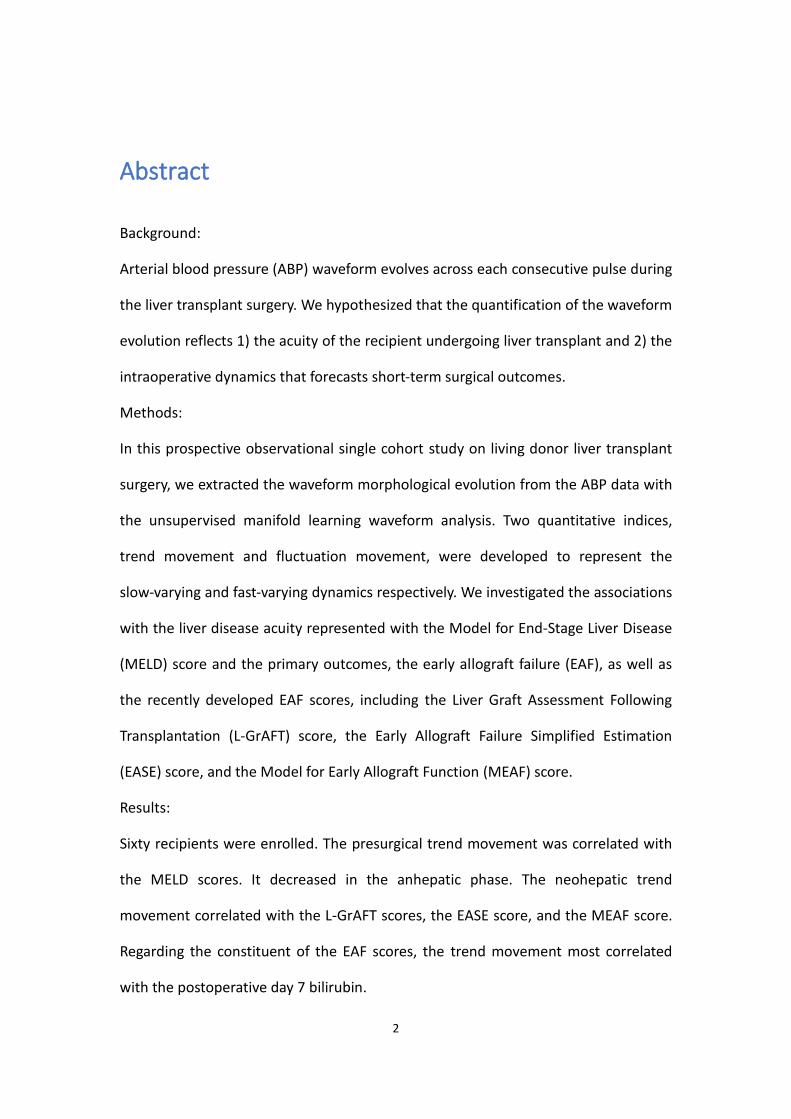
various system interactions1, 2. We incidentally observed that the arterial blood
pressure (ABP) waveforms during the liver transplant surgery contain a temporal
evolution phenomenon: recipients of favorable conditions possess richer intricacy in
their ABP waveform morphology evolution with time, and vice versa3 (Fig. 1).
The observation of waveform evolution between each consecutive pulse is enabled
by the unsupervised manifold learning technique we recently developed for
cardiovascular waveform analysis4, 5. By capturing subtle waveform morphological
change and condensing its information as a trajectory in a multivariate coordinate,
the Dynamic Diffusion Map (DDMap) technique offers 3-dimensional (3D) images for
visual inspection (Fig. 1). This technique has been employed in machine learning
tasks, including detecting ECG waveform for ischemic heart disease, as well as
presenting the ABP waveform dynamics in vasoactive episodes and noxious stimuli4-6.
In contrast to the “one representative waveform” approach exploited in clinical
4
scenarios to predict hypotension, to assess arterial stiffness, or to derive the profiles
of the cardiovascular system7-10, the waveform temporal evolution is a new
dynamical information among all consecutive pulses that has never been reported
before our incidental findings, which inspired us to further investigate as direct ABP
monitoring is mandatory during the transplant surgery.
To assess the liver disease acuity, researchers have employed laboratory data11 to
develop indices, including the Child-Pugh score, the Model for End-Stage Liver
Disease (MELD) score and MELD-Na score2, 12, 13 for years12, 14, 15. The success of
laboratory data combined with mathematical formula has led to the research in the
prediction of the Early Allograft Failure (EAF) outcome. We have seen the
development of EAF scores from the Model for Early Allograft Function (MEAF)
score14-18 and the Early Allograft Failure Simplified Estimation (EASE) score19 to the
recently-developed Liver Graft Assessment Following Transplantation (L-GrAFT)
scores20, 21 based on the laboratory data till postoperative day (POD) 10.
However, the crucial moment is still the surgery, during which the laboratory
examination inevitably falls behind the dynamical surgical progress and provides no
practical information regarding the present condition. To fill the void, we proposed to
exploit the temporal evolution intricacy phenomenon, which may reveal the
dynamical regulatory ability to maintain homeostasis in the cardiovascular system4.
Regarding this phenomenon, we proposed two intricacy indices, the trend
movement and fluctuation movement, to quantify the temporal evolution intricacy
during liver transplant surgery. We hypothesized that these indices are associated
with 1) the recipient’s acuity before the transplant surgery, 2) the transitions in
surgical phases from the presurgical phase to the anhepatic phase and neohepatic
phase, and 3) inference of the short-term surgical outcome in terms of the EASE,
MEAF, L-GrAFT7 and L-GrAFT10.
5
Fig. 1.
Arterial blood pressure (ABP) data and waveforms from 2 demonstration cases in
presurgical phase and in anhepatic phase show 4 pulse-by-pulse trajectories (thin
lines) and the trend movements (thick lines) in a 3-D image after the considered
manifold learning waveform analysis. The trajectories and trends representing ABP
temporal evolution in the 4 zoomed subfigures show high-dimensional (multivariate)
movements indicating complex pathophysiological interactions. Fading in color
indicates time direction. In the presurgical phase, case 1 (MELD score: 8) presents
more fluctuation movement and trend movement than case 2 (MELD score: 32).
Both movements decreased in anhepatic phase. Note that the 4 trajectories and

6
their trends move with multitude directions forming complex shape in 3-D space,
which is a simplified representation of their multi-dimensional (multivariate)
activities. (Supplementary videos at https://youtu.be/P9rId9xpl90 and
https://youtu.be/yu1rucN0S-4)
Material and Methods
Patients and methods
This is a single center prospective observational study between 2018 and 2021 in
Taipei Veterans General Hospital, Taipei, Taiwan. After Institutional Review Board
approval (IRB No.: 2017-12-003CC and 2020-08-005A) and written informed consent
obtained from each patient included in this study, 60 living donor liver recipients
(LDLR) were recruited. There were two reasons to select LDLR. First, living donors
from family members outnumbered cadaveric donors in Taiwan22 and second, the
variance in cold ischemia time of the graft was minimal. The study protocol conforms
to the ethical guidelines of the 1975 Declaration of Helsinki.
The latest laboratory data within one week before the elective surgery was used to
calculate the MELD score18 , MELD-Na score13 and Child-Pugh score2. The MELD
scores were used for patients awaiting liver transplantation to predict mortality and
to improve graft allocation. The original MELD score comprised 3 laboratory data,
including the total bilirubin, creatinine, and international normalized ratio (INR). The
revised MELD-Na score includes sodium as the fourth variable to improve its
performance.
The continuous physiological waveform signal data were collected from the patient
monitor (GE CARESCAPETM B850, GE Healthcare, Chicago, IL) via the data collection
software S5 Collect (GE Healthcare) from the liver transplant recipient who

7
underwent surgery during the whole surgical period. The physiological data,
including electrocardiogram (ECG), ABP, central venous pressure (CVP) and pulse
oximetry, were recorded from the start of the anesthetic maintenance through the
whole surgery, but only ABP was used in the upcoming analysis. The recorded
waveforms were uniformly sampled at 300 Hz. In addition, we routinely set a
portocaval shunt during the anhepatic phase to release the portal flow and the
congestion of the intestine. We registered the specific time points, including the
hilum clamp before hepatectomy, end of the hepatectomy, portocaval shunt
establishment, portal vein reperfusion, hepatic artery reperfusion, and completion of
bile duct anastomosis. After the operation, the liver recipients were transferred to
the Intensive care unit (ICU) where the postoperative recovery was under the
discretion of physicians in ICU, who were blinded of this study.
The main clinical outcome is the graft failure determined by patient death or liver
retransplantation within 3 months20. The prognostic condition following
transplantation were evaluated by 4 recently developed EAF scores20, including the
MEAF score16, the L-GrAFT7 and L-GrAFT10 scores, as well as the EASE score19. The
MEAF score comprised alanine aminotransferase (ALT), the international normalized
ratio (INR), and the bilirubin data. The L-GrAFT7 score and L-GrAFT10 score comprised
the laboratory data of AST, INR, total bilirubin, and platelet counts at day 7 and day
10 respectively. In comparison with the above scores, the EASE score consumed
more items, including the laboratory data of aspartate aminotransferase (AST),
platelet, bilirubin within 10 days, as well as the MELD score, the number of
transfused packed red blood cell during surgery, the events of vascular thrombosis
within 10 days after the surgery and whether the early volume of the institution is
larger than 70 cases per year. It is apparent that the bilirubin, AST, PLT and INR are
the common constituents of the above EAF scores. Per institutional routine,
8
recipients underwent daily venous blood check within POD7. Afterward recipients of
good recovery at the discretion of the surgeon would be checked for every other day.
The missing data point is imputed by a linear regression method under the
assumption that the laboratory information is changing individually and localized in
time.
Waveform data selection and processing
We chose 3 surgical phases for data analysis, the presurgical phase, the anhepatic
phase and the neohepatic phase. The presurgical phase data were chosen when the
anesthetic maintenance started and the preparation for the imminent surgery was
undergoing as it represented the baseline condition without the surgical stimulation.
We chose the first 800 ABP pulses from each recipient, which amounted to less than
10 minutes of data collection period in the presurgical phase, as the representation
of the recipient’s condition with the old liver. The anhepatic phase data were chosen
as a 10-minute period after the portocaval shunt had been established. We inspected
the waveform to ascertain neither drastic change nor severe artifact during this
10-minute period. The consideration of the constant 10-minute period approach
would be more suitable for standardization for future research. The neohepatic
phase data were chosen as a hemodynamically stable 10-minute period after the
anastomosis of the biliary duct, and before the abdominal wound closure was
performed. During this period, the reperfusion and the re-establishment of the
hepatic artery flow had performed, and the new liver graft was supposed to have
functioned for a while.
To prepare the consecutive ABP waveform pulses for the manifold learning (Fig. 1),
we use the maximum of the systolic phase slope as the fiducial point to obtain each
pulse cycle4. Legitimate ABP pulses were automatically detected and extracted based

9
on the following criteria: the pulse width, the extreme value, the pulse pressure, the
duration between two successive pulses should be within reasonable limits, which
are determined inter-individually and dynamically. As the heart rate is time-varying,
the pulse count and the time duration are not linearly related. It is worth noting that
we chose the 800-pulse data in the presurgical phase for the uniform contribution
from each case.
Unsupervised manifold learning and Intricacy quantification
The pulse-by-pulse ABP waveform temporal evolution is too subtle to be directly
gauged by the naked eye. We use the unsupervised manifold learning algorithm,
DDMap, to condense the waveform information for visualization and quantification.
After the above-mentioned pre-processing procedure, we treat those consecutive
pulses as high dimensional data points and finds a geometric structure (the manifold)
in the high dimensional space representing the trajectory of the waveforms evolving
with time (Fig. 1).
The main technical innovation, in a nutshell, is measuring every waveform by all the
other waveforms as the gauges. That is, the knowledge gained from this method is
the united contribution of the waveform data, which also supports the robustness
(less susceptible to the noise). In the frame of unsupervised machine learning, this
method consumes only the successive pulse-to-pulse waveform morphology without
the input of time labeling, medical history, lab test data, or the surgical procedure.
This data-centered agnostic approach allows us to represent the waveform evolution
in a more comprehensive manner4.
While DDMap provides a concise overview of the complex dynamical evolution of
ABP waveforms, the trajectory consisting of consecutive pulses forms a unique shape
that cannot be simply measured from the raw ABP waveform (Fig. 1, Fig. S1). Our
past studies and other lines of evidence support that ABP waveforms are determined
by several factors including the vascular tone, cardiac contractility, and preload. A
simple noxious stimulus will elicit multiple reflexes producing a complex trajectory
shape in high dimensional space4. Our empirical findings that the more waveform

10
evolution intricacy is associated with a better condition justifies the employment of
the manifold learning. The main feature we observed is that the trajectory consists of
a trend (slowly varying) and fluctuation (fast varying) in the high dimensional space.
We proposed two indices to quantify the intricacy; the fluctuation movement
quantifies the fast-varying evolution, and the trend movement quantifies the
slow-varying evolution (Fig. S1). Both indices were designed to range roughly from
0-100 based on the median value and the interquartile range (IQR) of the data in this
study. More technical information is presented in the supplementary.
Validation analysis
Sensitivity analysis was performed to evaluate the effect of parameter selection.
Since both indices, the trend movement and the fluctuation movement, are based on
the trajectory analysis, we investigate the effect of different filtering length K in ABP
intricacy quantification.
To further validate our hypothesis of temporal intricacy in the ABP waveform
morphology, we employed different null models. The random perturbation of the
time sequence labeling was designed to validate the ABP temporal evolution
intricacy; the perturbation of case labeling of the ABP waveform data was designed
to validate our hypothesis between ABP waveform evolution and the liver disease
acuity; the perturbation by replacing each pulse wave with each mean blood
pressure value was to validate the waveform morphological information.
Statistical analysis
We explored three clinical information by the proposed intricacy indices. The first
one was directly evaluating the correlation between the intricacy indices and the
MELD scores in the presurgical phase. The second one was the intricacy evolution
from the anhepatic phase to neohepatic phase. The rationale is that the ability to
11
dynamically reflect the drastic pathophysiological effect from the presurgical to the
anhepatic phase should present as the variation in the correlation with the MELD
scores. Third, we investigated how the intricacy indices in the neohepatic phase are
associated with the EAF scores and their constituents.
Pearson correlation was used to establish the association between the intricacy
indices and the clinical condition. The bootstrap resampling without replacement for
statistical inference was used for exemption from the normal distribution assumption.
The 95% confidence interval (CI) of each considered statistic was derived from the
bootstrap resampling without replacement with 100,000 resamples. Note that a
higher MELD score represents a worse acuity while we hypothesize that a higher
intricacy reflects better homeostasis of the human body, so the ideal correlation
coefficient is -1. It is the same case with any other quantity representing the worse
condition with a higher value. The association of indices with other scores or factors
was further evaluated with multivariate regression, where the relative importance of
each factor is derived from the R square. The demographic data and laboratory data
were expressed as median (1st quartile, 3rd quartile and interquartile range (IQR)).
Statistical results are expressed as mean and its 95% CI. Null hypothesis test was
considered significant when the P value < 0.05.
We performed the waveform data processing and manifold learning with C#
language (Visual Studio community 2019, Microsoft, Redmond, WA), and the
statistical analyses with R (version 4.1.0; the R Foundation for Statistical Computing).
The calculation of MELD, MELD-Na, and EAF scores were performed with
spreadsheet software Excel (Microsoft, Redmond, WA), where each formula was
sourced from each corresponding author. MELD and MELD-Na were calculated
without rounding off decimals to avoid the round-off error. IQRs of ABP intricacy
indices and descriptive statistics were evaluated by the quantile function of R

12
language in type 8 algorithm per R documentation recommendation.
Results
Among the 60 enrolled patients, the main indications for liver transplant are acute
viral hepatitis and hepatocellular carcinoma (table 1). The acuity of liver disease is
relatively mild (MELD-Na: 20.4 [14.4, 31.1]). The MEAF score is 6.21(4.52,7.43,
IQR=2.91); the L-GrAFT7 score is -2.54 (-3.12, -1.69, IQR=1.44); the L-GrAFT10 score is
-2.45 (-2.97, -1.32, IQR=1.6); the EASE score is -2.19 (-2.84, -1.60, IQR=1.24). There
are 5 EAFs (5 mortality, no retransplantation) within POD40. There were 3 cases
lacking anhepatic ABP data and 2 cases lacking neohepatic ABP data due to technical
issues during the data recording.
Presurgical ABP intricacy and the acuity condition
In the presurgical phase, both ABP intricacy indices correlate with MELD score and
MELD-Na scores (Fig.2 and supplementary Fig. S2, S3). For the fluctuation movement,
the Pearson correlation coefficients (CC) with MELD-Na and MELD score are -0.485
(-0.303, -0.638) and -0.468 (-0.280, -0.625) respectively, whereas for the trend
movement, the CC with MELD-Na and MELD scores are -0.505 (-0.327, -0.650) and
-0.488 (-0.299, -0.640) respectively. All 4 correlations show p < 0.0001. In addition,
the trend movement and fluctuation movement are also correlated with Child-Pugh
scores with the Pearson CC -0.442(-0.221, -0.619, P=0.00015) and -0.330 (-0.106,
-0.542, P=0.0023) respectively.
In the sensitivity analysis, ABP intricacy indices being derived from various
parameters consistently shows higher MELD-Na score correlation than the MELD

13
score (Fig. S2). Detailed results of the sensitivity analysis and the validation of the
quantitative indices are presented in the supplementary.
Fig. 2. The correlation of trend movement (Mov) and fluctuation movement with
MELD (Model for End-Stage Liver Disease) and MELD-Na scores in the presurgical
phase. The Pearson correlation coefficients, 95% confidence intervals (error bars) and
p values in the presurgical, anhepatic, and neohepatic phases are shown. Trend
movement correlates best in the presurgical phase but not in the subsequent phases,
14
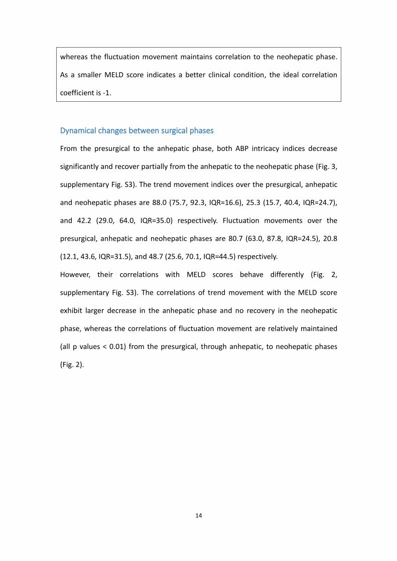
whereas the fluctuation movement maintains correlation to the neohepatic phase.
As a smaller MELD score indicates a better clinical condition, the ideal correlation
coefficient is -1.
Dynamical changes between surgical phases
From the presurgical to the anhepatic phase, both ABP intricacy indices decrease
significantly and recover partially from the anhepatic to the neohepatic phase (Fig. 3,
supplementary Fig. S3). The trend movement indices over the presurgical, anhepatic
and neohepatic phases are 88.0 (75.7, 92.3, IQR=16.6), 25.3 (15.7, 40.4, IQR=24.7),
and 42.2 (29.0, 64.0, IQR=35.0) respectively. Fluctuation movements over the
presurgical, anhepatic and neohepatic phases are 80.7 (63.0, 87.8, IQR=24.5), 20.8
(12.1, 43.6, IQR=31.5), and 48.7 (25.6, 70.1, IQR=44.5) respectively.
However, their correlations with MELD scores behave differently (Fig. 2,
supplementary Fig. S3). The correlations of trend movement with the MELD score
exhibit larger decrease in the anhepatic phase and no recovery in the neohepatic
phase, whereas the correlations of fluctuation movement are relatively maintained
(all p values < 0.01) from the presurgical, through anhepatic, to neohepatic phases
(Fig. 2).
15
Fig 3. The trend movements (left panel) and fluctuation movements (right panel)
from all cases (60) colored as grayscale lines (darker in higher MELD-Na score) show
evolutions among the presurgical, anhepatic, and neohepatic phases. The medians
are superimposed in blue and 5 early-allograft-failure (EAF) cases marked by red
dotted lines (survival days < 14 days) and yellow dotted lines (survival days > 14 days)
are also superimposed. The legend is labeled with the MELD-Na score, where the
letter E represents EAF and the following number represents survival days. The graph
shows the main findings in this study: 1) higher trend movements in the presurgical
phase are associated with lower MELD scores, 2) indices decreased in the anhepatic
phase, 3) indices partially recovered in the neohepatic phase, and 4) there is an
association of EAF outcome and ABP intricacy at the neohepatic phase.
Association with the surgical outcomes
Five EAF cases present lower trend movements (EAF: 27.2 [9.3, 29.3, IQR=20.0];

16
non-EAF: 42.8 [33.2, 64.8, IQR=31.6]) and lower fluctuation movements (EAF: 16.3
[12.6, 27.9, IQR=15.4]; non-EAF: 49.9 [27.6, 70.7, IQR=43.1]) than 55 non-EAF cases.
Regarding the EAF scores, MEAF score is higher in EAF cases (EAF: 8.30 [7.44, 8.57,
IQR=1.13]; non-EAF: 5.95 [4.53, 7.02, IQR=2.48]; p=0.07). The 5 EAF cases also
present higher L-GrAFT7 score (EAF: 0.0824 [-1.80, 2.19, IQR=3.98]; non-EAF: -2.57
[-3.12, -1.82, IQR=1.30]; p=0.06) and L-GrAFT10 (EAF: 1.16 [-0.576, 3.99, IQR=4.57];
non-EAF: -2.52 [-2.97, -1.64, IQR=1.33]; p=0.05) while the hypothesis test is marginal.
The EASE score is consistent with the above (EAF: 1.85 [0.660, 2.01, IQR=2.68];
non-EAF: -2.24 [-2.81, -1.63, IQR=1.17]; p=0.29).
The strongest association of intricacy indices with EAF scores during the neohepatic
phase happens when the trend movement and either L-GrAFT score are considered
(Fig. 4). Over the neohepatic phase, the trend movement significantly correlates with
the L-GrAFT7 score (CC=-0.382 [-0.122, -0.579], P=0.0038), and the L-GrAFT10 score
(CC=-0.398 [-0.142, -0.598], P=0.0027) while the correlations between the
fluctuation movement and L-GrAFT scores are marginal significant. The correlation
between the trend movement and EASE score is marginal while there are no
correlations between the intricacy indices and MEAF score.

17
Fig.4. Correlations between neohepatic trend and fluctuation movements with
early-allograft-failure (EAF) scores, including MEAF (Model for Early Allograft
Function) score, the Liver Graft Assessment Following Transplantation risk score in
day 7 (L-GrAFT7) and in day 10 (L-GrAFT10), and the Early Allograft Failure Simplified
Estimation (EASE) score. Error bars indicate 95% confidence intervals. L-GrAFT7 and
L-GrAFT10 scores correlate better with the trend movement than the other EAF
scores and fluctuation movements.
For laboratory data as constituents of EAF scores (Fig. 5), the association with
neohepatic trend movements increases day by day. Both total bilirubin and direct
bilirubin reach peaks at day 8 (total bilirubin: CC=-0.370 [-0.104, -0.583], P=0.004;
18
direct bilirubin: CC=-0.386 [-0.113, -0.603], P=0.004) (Fig. 5). The second best
neohepatic trend movement correlation is the platelet count, which reaches peak at
day 5 with a marginal significance (CC=0.348 [0.587, 0.077], P=0.006). In contrast, the
correlations of the neohepatic fluctuation movement and the bilirubin reach peak at
day 2 (total bilirubin: CC=-0.338 [-0.097, -0.535], P=0.004; direct bilirubin: CC=-0.326
[-0.094, -0.517], P=0.004) and decrease afterwards. It is worth noting that the
correlation between the trend movement and AST peaks at POD3.
Predict ABP intricacy with MELD score and demographic factors
To predict the presurgical intricacy indices by the MELD-Na score and demographic
data, the linear regression analysis shows MELD-Na is the most significant factor for
the trend movements (t=-5.08, p<0.00001, relative importance: 88%), followed by
age (t=-2.00, p=0.0498, relative importance: 12%). The BMI and gender are
non-significant. Combining all 4 factors in linear regression leads to adjusted
R-squared: 0.337 (p<0.00001). For the fluctuation movement, the regression analysis
also shows MELD-Na is the most significant factor (t=-4.17, p=0.0001, relative
importance: 73%), followed by age (t=-2.61, p=0.011, relative importance: 27%). The
BMI and gender are not significant.
Sensitivity analysis and validation analyses
The sensitivity analysis shows that the derivation of both indices is robust and
insensitive to parameter selection (supplementary Fig. S2, S3). The validation analysis
against Null model (Fig. S4) shows decreased association between the meld scores
and the presurgical ABP data when the waveform morphology information or the
time sequence information was removed. The null model of case labeling shows no
association with the MELD scores. The detail results are in the supplementary.

19
Fig.5.
The Pearson correlations of the neohepatic ABP intricacy indices with respect to the
post-surgical laboratory data as the constituent of the early-allograft-failure scores.
Arrows indicate the maximal correlation of total bilirubin (TB) and direct bilirubin
(DB) on day 8 and the “negative” platelet count (nPLT) on day 5. The nPLT is to make
the platelet count correlation the same direction with all other data for better
visualization here as higher platelet means better condition. There are no significant
correlations of the alanine aminotransferase (ALT), aspartate aminotransferase (AST),
and the international normalized ratio (INR).

20
Table 1. The demographic data
Characteristics Number (%) Median (IQR) Mean (SD)
Age, year NA 57 (52–62) 56.5 (8.4)
Male sex 45 (76.3) NA NA
Main indication
Viral hepatitis B 36 (61) NA NA
Viral hepatitis C 7 (11.9) NA NA
Alcoholic cirrhosis 9 (15.3) NA NA
Other 5 (8.5) NA NA
HCC 33 (55.9) NA NA
MELD NA 18.3 (13.5–28.6) 21.0 (11.1)
MELD-Na NA 20.4 (14.4–31.1) 22.6 (10.7)
GRWR, % NA 1.01 (0.88–1.21) 1.11 (0.34)
CIT, min NA 65 (44–96) 76.8 (42.5)
WIT, min NA 41 (32–54) 44.4 (14.9)
Graft data
Type
RL without MHV, con(-) 27 (45.0) NA NA
RL without MHV, con(+) 23 (38.3) NA NA
RL with MHV 2 (3.3) NA NA
LL with MHV 8 (13.3) NA NA
Fatty liver, macrovesicular,
%
NA NA
None 25 (41.7) NA NA
1~10 25 (41.7) NA NA

21
11~20 8 (13.3) NA NA
21~30 2 (3.3) NA NA
CIT: cold ischemia time; GRWR: graft-to-recipient weight ratio; HCC: hepatocellular
carcinoma; LL: left lobe; MELD: model of end stage liver disease; MHV: middle
hepatic vein; RL: right lobe; WIT: warm ischemia time.
22
Discussion
This is the first study that investigates the pulse-by-pulse temporal evolution of ABP
waveform in liver transplant surgery by an unsupervised manifold learning technique.
We showed that the ABP intricacy reflects 1) the presurgical condition, 2) the
transition between surgical phases, and 3) the early surgical outcome contribution.
These support the association between a favorable condition and more ABP
waveform evolution intricacy, which is dynamic within a liver transplant surgery. The
association between intraoperative ABP waveform and surgical outcome is beyond
our expectations.
Presurgical condition
The MELD and MELD-Na scores are used for ranking the urgency of patients awaiting
liver transplant surgery. It is also useful for the assessment of various liver diseases,
which were formerly served by the Child-Pugh score.2 Our presurgical results (Fig. 2)
show the correlation in the order of the MELD-Na, MELD and Child-Pugh score,
which is consistent with the chronological advancement of the above scores
developed. It is known that conditions before the transplant surgery do not
represent the liver transplant surgical outcome2, 23. In our data, the neohepatic trend
movement shows no association with the presurgical condition and the presurgical
trend movement shows no association with the EAF scores. Our result and evidence
suggest that during the presurgical period after the anesthetic induction and before
the surgery, the ABP data might be a window to peek into the baseline condition (Fig.
1, Fig. 2). We postulate that patients with lower (better) MELDs possess more
homeostatic capability in their cardiovascular system, and thus their ABP waveform
23
reflects more temporal intricacy.
Transitions in surgical phases
During the anhepatic phase, although we reconstructed the portocaval shunt to
release the portal flow, a functioning liver does not exist. The intricacy indices were
decreased, especially the trend movement, which recovers partially in the
neohepatic phase (Fig. 3). The correlations between the MELD scores and the trend
movement were also decreased (Fig. 2). These suggest that the trend movement
reflects the dynamics of the pathophysiological condition. In contrast, the correlation
between the MELD scores and the fluctuation movement is relatively preserved in
the anhepatic and neohepatic phase. This property is not favorable for surgical
outcome assessment but worth investigation in the future.
EAD, MEAF, L-GrAFT scores and their constituents
As the presurgical MELD and MELD-Na are not representative of the surgical
outcome, laboratory data such as bilirubin have been intensively investigated to
assess the graft outcome1, 11. To extract the underlying information, the EAF scores
utilizes not one single spot value, but information from multiple values processed by
mathematical formulas involving the area-under-curve summation, maximum, slope
and logistic function19-21. Our results show that the neohepatic trend movement is
correlated with the L-GrAFT7, L-GrAFT10, and EASE, but not MEAF score (Fig. 4). It is
worth noting that the MEAF score is derived from the laboratory data within POD3
after surgery, including ALT, INR, and bilirubin, while the other later-developed EAF
scores weigh more on the laboratory data between POD3 to POD10 and achieve
better prognostic performance1, 20, 24. Moreover, the additional accuracy of L-GrAFT10
score consuming 3 more days laboratory than the L-GrAFT7 score also justifies the
slight better correlation with L-GrAFT10 than that with L-GrAFT7 score (Fig.4) in this
24
study. These lines of evidence suggest the connection between intraoperative ABP
intricacy and the surgical outcome assessment scores.
Regarding the constituent analyses, the trend movement also correlates best with
the POD8 direct bilirubin and indirect bilirubin (Fig. 5), which is similar to the finding
reported by Olthoff et al1. regarding the POD7 bilirubin > 10mg/dl as one indicator of
early graft dysfunction. The authors suggested it represents the graft function rather
than the pre-surgical condition. The peak performance with POD8 bilirubin in our
study is also in line with the better L-GrAFT10 accuracy than L-GrAFT7, as L-GrAFT10
contains POD8 bilirubin information. Our result regarding the correlation between
POD5 platelet count and the ABP intricacy is in agreement with the previous
researches25, 26, where the authors reported that thrombocytopenia (platelet counts
< 72500/μL) on POD5 as an independent factor for EAF. Takahashi et al. 28 suggested
that the prognostic effect of thrombocytopenia cannot be simply attributed to
presurgical conditions or the postoperative graft function. The platelet may promote
liver regeneration. Our result of the correlation between the AST and the trend
movement peaks at POD3 (Fig. 5) is in agreement with the prognostic value of POD3
AST, but not POD3 ALT, reported by Robertson et al. in a large scale prospective
study24, 27 . However, our result is not significant in statistics probably due to the scale
of our case number or the minimal ischemia time of the living donor liver transplant.
In summary, the constituent analysis results support the association between the
intraoperative ABP intricacy and the graft function recovery, which takes days to
reflect in the laboratory data.
Pathophysiology and clinical implication
Our results show the ABP intricacy in transplant surgery associated with the
presurgical condition, surgical phase transition, outcome scores, and prognostic

25
laboratory data, the bilirubin and platelet count. Literatures indicated the ABP
waveform reflecting information of arterial stiffness, imminent shock, and
cardiovascular system profile7-10. Our past study showed the effect of vasoactive
medication or noxious stimulation in ABP waveform via manifold learning4. These
lines of evidence suggest the regulating mechanism involving multiple organs or
systems. To our best knowledge, there is no literature reporting relevant findings.
However, a similar notion that more variability or complexity is associated with
better vitality has been reported in other biomedical data. The beat-to-beat heart
rate variability (HRV) extracted from ECG has been long known to be associated with
the autonomic nerve activity, where a larger variability is in general associated with a
better outlook28, 29. The blood pressure variability and breathing pattern variability
also possess similar notions.30 Our null model tests (Fig. S4) shed some light on the
blood pressure variability. Replacing waveform with mean blood pressure and
perturbating the time sequence information reduce the ABP evolution intricacy to
the blood pressure variation. The decreased association with the MELD scores
suggests that the waveform morphology information and time sequence information
are vital to the evolution intricacy.
On the other hand, it is also known that the renin–angiotensin–aldosterone system is
a hormone system regulating the vascular tone, fluid status and electrolyte while the
liver produces angiotensinogen. The system possibly contributes the ABP temporal
evolution phenomenon. We speculate the regulatory mechanism to maintain
homeostasis underpinning these phenomena31. Our result shows that age is also a
significant factor of the evolution intricacy while aging is known to diminish the
homeostatic regulation. Since the homeostasis physiology involves multiple organs
and systems, it is not a trivial task investigating the pathophysiology. The present
results also implicate the possible clinical merit in outcome forecast or as an

26
“real-time liver function index”. A potential parallel to the laboratory examination
warrants future clinical study.
Methodological considerations
The temporal evolution intricacy of ABP waveform is an obscure physiological
phenomenon. As the pulse-by-pulse change is subtle and complicated, it cannot be
easily seen and summarized with naked eyes (Fig.1, Fig. S1). Our results justify the
employment of the unsupervised manifold learning method to extract this intricacy
information. The ABP waveform analysis has been implicated in hemodynamic
problems, ranging from predicting hypotension9, assessing hemodynamic status7, 32-34,
and guiding medical treatment for chronic hypertension8, 10. Most existing ABP
waveform analysis techniques, including those embedded in monitoring instruments,
require collapsing data within a time frame to obtain a “representative” waveform
and/or determine landmark-dependent features. However, as the status of the
cardiovascular system is ever-changing, the temporal evolution intricacy information
might be collapsed by those techniques. Our previous study4, 5 suggests that any
perturbation on the ABP waveform and the subsequent response inevitably produce
changes in multiple scales (for example vasoconstriction and cardiac contractility
pertain to different scales), which render the basic statistical entities, such as the
average or the variance, based on one dimensional scale impractical. Hence, it
justifies employing manifold learning to ABP waveform evolution in high-dimensional
(multivariate), from which the intricacy indices quantify the overall effect of multiple
regulatory mechanisms on ABP waveform morphology. The other advantage is a
visualization that helps “grasp the whole picture” to establish the concrete structure
in our mind. The 3-D image inspired us to use the notion of movement from the
Newtonian mechanics to quantify the trajectory (Fig. 1, Fig. S1).

27
Limitation and Future Works
There are several limitations in this study. Our EAF case number (5) is not large
enough to reach statistical significance with respect to non-EAF group despite the
difference in the descriptive statistics. A larger scale study is needed for further
factor analysis. Second, we did not collect the postoperative waveform data. As the
intra-operative neohepatic ABP information associates with the EAF scores, it is
intriguing to suspect that the ABP data during postoperative recovery offer more
definite outcome information. Third, our result is obtained from living donor liver
transplant. It maybe not representative to cadaver liver transplant as the cold
ischemia time is incomparable. Fourth, our methodology involves ABP waveform
recording hence it may not be feasible for retrospective research, as most electronic
medical records systems do not include waveform data.
In future study, the ABP intricacy in postoperative recovery period deserves to be
elucidated. As the surgical phase transition from the anhepatic to neohepatic phase
prognosticates the surgical outcome much earlier than the laboratory data, it is
mandatory to investigate the possibility of outcome improvement by the timely
intraoperative intervention or the early intervention during postoperative recovery.
In light of the EAF scores, forthcoming analyses combining ABP evolution and other
laboratory data is warranted. We envision the development of an integrated solution
for the early outcome prediction and even risk modification via timely assessment in
clinical liver transplantation ultimately.
Conclusion
The quantitative intricacy in successive ABP waveform evolution reflects the liver
disease severity, dynamically indicates the liver transplant steps, and foretells the
short-term surgical outcomes.

28
Acknowledgement
We thank Professor Alfonso Avolio (UCSC, Italy) for kindly providing the details of the
EASE score calculation and we thank Professor Vatche G. Agopian (UCLA, US) for
kindly providing the details of the L-Graft scores calculations.
This study was supported by the National Science and Technology Development Fund
(MOST 109-2115-M-075 -001) of Ministry of Science and Technology, Taipei, Taiwan,
References
1. Olthoff KM, Kulik L, Samstein B, Kaminski M, Abecassis M, Emond J, Shaked A
and Christie JD. Validation of a current definition of early allograft dysfunction in liver
transplant recipients and analysis of risk factors. Liver Transplantation.
2010;16:943-949.
2. Brown Jr RS, Kumar KS, Russo MW, Kinkhabwala M, Rudow DL, Harren P,
Lobritto S and Emond JC. Model for end-stage liver disease and Child-Turcotte-Pugh
score as predictors of pretransplantation disease severity, posttransplantation
outcome, and resource utilization in United Network for Organ Sharing status 2A
patients. Liver Transplantation. 2002;8:278-284.
3. Y.-T. Lin H-TW, S.-C. Wang, C.-K. Ting, C. Liu, N.-C. Lin, C.-Y. Chen, and C.-C. Loong. .
Intraoperative arterial pressure waveforms shows temporal structure complexity
correlated with acuity of liver transplant by pulse wave manifold learning analysis.
Paper presented at: Society for Technology in Anesthesia, Virtual Annual Meeting,
2021; 2021; Online.
4. Wang S-C, Wu H-T, Huang P-H, Chang C-H, Ting C-K and Lin Y-T. Novel imaging

29
revealing inner dynamics for cardiovascular waveform analysis via unsupervised
manifold learning. Anesthesia & Analgesia. 2020;130:1244-1254.
5. Lin Y-T, Malik J and Wu H-T. Wave-shape oscillatory model for nonstationary
periodic time series analysis. Foundations of Data Science. 2021.
6. Lin Y-T, Lin T-S, Wu H-t, Chang C-H, Wang S-C and Chien-Kun T. Tracking Dynamic
Arterial Pressure Waveform on Vasoactive Medication Via Manifold Learning Method.
ANESTHESIA AND ANALGESIA. 2019;128:0-0.
7. Sluyter JD, Hughes AD, Camargo Jr CA, Thom SAM, Parker KH, Hametner B,
Wassertheurer S and Scragg R. Identification of Distinct Arterial Waveform Clusters
and a Longitudinal Evaluation of Their Clinical Usefulness. Hypertension.
2019;74:921-928.
8. Chen C-H, Nevo E, Fetics B, Pak PH, Yin FC, Maughan WL and Kass DA.
Estimation of central aortic pressure waveform by mathematical transformation of
radial tonometry pressure: validation of generalized transfer function. Circulation.
1997;95:1827-1836.
9. Hatib F, Jian Z, Buddi S, Lee C, Settels J, Sibert K, Rinehart J and Cannesson M.
Machine-learning Algorithm to Predict Hypotension Based on High-fidelity Arterial
Pressure Waveform Analysis. Anesthesiology. 2018;129:663-674.
10. Avolio AP, Van Bortel LM, Boutouyrie P, Cockcroft JR, McEniery CM, Protogerou
AD, Roman MJ, Safar ME, Segers P and Smulyan H. Role of pulse pressure
amplification in arterial hypertension: experts' opinion and review of the data.
Hypertension. 2009;54:375-83.
11. Marubashi S, Dono K, Nagano H, Asaoka T, Hama N, Kobayashi S, Miyamoto A,
Takeda Y, Umeshita K and Monden M. Postoperative Hyperbilirubinemia and Graft
Outcome in Living Donor Liver Transplantation. Liver transplantation: official
publication of the American Association for the Study of Liver Diseases and the
30
International Liver Transplantation Society. 2007;13:1538-1544.
12. Kim WR, Biggins SW, Kremers WK, Wiesner RH, Kamath PS, Benson JT, Edwards E
and Therneau TM. Hyponatremia and mortality among patients on the
liver-transplant waiting list. New England Journal of Medicine. 2008;359:1018-1026.
13. Biggins SW, Kim WR, Terrault NA, Saab S, Balan V, Schiano T, Benson J, Therneau
T, Kremers W, Wiesner R, Kamath P and Klintmalm G. Evidence-based incorporation
of serum sodium concentration into MELD. Gastroenterology. 2006;130:1652-60.
14. Leise MD, Kim WR, Kremers WK, Larson JJ, Benson JT and Therneau TM. A
revised model for end-stage liver disease optimizes prediction of mortality among
patients awaiting liver transplantation. Gastroenterology. 2011;140:1952-1960.
15. Kamath PS and Kim WR. The model for end‐stage liver disease (MELD).
Hepatology. 2007;45:797-805.
16. Pareja E, Cortes M, Hervás D, Mir J, Valdivieso A, Castell JV and Lahoz A. A score
model for the continuous grading of early allograft dysfunction severity. Liver
Transplantation. 2015;21:38-46.
17. Said A, Williams J, Holden J, Remington P, Gangnon R, Musat A and Lucey MR.
Model for end stage liver disease score predicts mortality across a broad spectrum of
liver disease. Journal of hepatology. 2004;40:897-903.
18. Kamath PS, Wiesner RH, Malinchoc M, Kremers W, Therneau TM, Kosberg CL,
D'Amico G, Dickson ER and Kim WR. A model to predict survival in patients with
end-stage liver disease. Hepatology. 2001;33:464-70.
19. Avolio AW, Franco A, Schlegel A, Lai Q, Meli S, Burra P, Patrono D, Ravaioli M,
Bassi D and Ferla F. Development and validation of a comprehensive model to
estimate early allograft failure among patients requiring early liver retransplant.
JAMA surgery. 2020;155:e204095-e204095.
20. Agopian VG, Markovic D, Klintmalm GB, Saracino G, Chapman WC, Vachharajani

31
N, Florman SS, Tabrizian P, Haydel B and Nasralla D. Multicenter validation of the liver
graft assessment following transplantation (L-GrAFT) score for assessment of early
allograft dysfunction. Journal of hepatology. 2021;74:881-892.
21. Agopian VG, Harlander-Locke MP, Markovic D, Dumronggittigule W, Xia V, Kaldas
FM, Zarrinpar A, Yersiz H, Farmer DG and Hiatt JR. Evaluation of early allograft
function using the liver graft assessment following transplantation risk score model.
JAMA surgery. 2018;153:436-444.
22. Lin YP, Chen J, Lee WC, Chiang YJ and Huang CW. Understanding family dynamics
in adult‐to‐adult living donor liver transplantation decision‐making in Taiwan:
Motivation, communication, and ambivalence. American Journal of Transplantation.
2021;21:1068-1079.
23. Rana A, Hardy M, Halazun K, Woodland D, Ratner L, Samstein B, Guarrera J,
Brown Jr R and Emond J. Survival outcomes following liver transplantation (SOFT)
score: a novel method to predict patient survival following liver transplantation.
American Journal of Transplantation. 2008;8:2537-2546.
24. Elsayed F, Sholkamy A, Elshazli M, Elshafie M and Naguib M. Comparison of
different scoring systems in predicting short-term mortality after liver transplantation.
Transplantation proceedings. 2015;47:1207-1210.
25. Lesurtel M, Raptis DA, Melloul E, Schlegel A, Oberkofler C, El‐Badry AM, Weber
A, Mueller N, Dutkowski P and Clavien PA. Low platelet counts after liver
transplantation predict early posttransplant survival: the 60‐5 criterion. Liver
Transplantation. 2014;20:147-155.
26. Takahashi K, Nagai S, Putchakayala KG, Safwan M, Li AY, Kane WJ, Singh PL,
Collins KM, Rizzari MD and Yoshida A. Prognostic impact of postoperative low platelet
count after liver transplantation. Clinical transplantation. 2017;31:e12891.
27. Robertson FP, Bessell PR, Diaz‐Nieto R, Thomas N, Rolando N, Fuller B and

32
Davidson BR. High serum Aspartate transaminase levels on day 3 postliver
transplantation correlates with graft and patient survival and would be a valid
surrogate for outcome in liver transplantation clinical trials. Transplant International.
2016;29:323-330.
28. Electrophysiology TFotESoCtNASoP. Heart rate variability: standards of
measurement, physiological interpretation, and clinical use. Circulation.
1996;93:1043-1065.
29. Lin Y and Wu H. ConceFT for Time-Varying Heart Rate Variability Analysis as a
Measure of Noxious Stimulation During General Anesthesia. IEEE transactions on
bio-medical engineering. 2017;64:145.
30. Stergiou GS, Parati G, Vlachopoulos C, Achimastos A, Andreadis E, Asmar R,
Avolio A, Benetos A, Bilo G and Boubouchairopoulou N. Methodology and
technology for peripheral and central blood pressure and blood pressure variability
measurement: current status and future directions–position statement of the
European Society of Hypertension Working Group on blood pressure monitoring and
cardiovascular variability. Journal of hypertension. 2016;34:1665-1677.
31. Fossion R, Rivera AL and Estañol B. A physicist’s view of homeostasis: how time
series of continuous monitoring reflect the function of physiological variables in
regulatory mechanisms. Physiological measurement. 2018;39:084007.
32. Biancofiore G, Critchley LA, Lee A, Yang X-x, Bindi LM, Esposito M, Bisà M,
Meacci L, Mozzo R and Filipponi F. Evaluation of a new software version of the
FloTrac/Vigileo (version 3.02) and a comparison with previous data in cirrhotic
patients undergoing liver transplant surgery. Anesthesia & Analgesia.
2011;113:515-522.
33. Shih B-F, Huang P-H, Yu H-P, Liu F-C, Lin C-C, Chung P-H, Chen C-Y, Chang C-J and
Tsai Y-F. Cardiac output assessed by the fourth-generation arterial waveform analysis

33
system is unreliable in liver transplant recipients. Transplantation proceedings.
2016;48:1170-1175.
34. Tsai Y, Su B, Lin C, Liu F, Lee W and Yu H. Cardiac output derived from arterial
pressure waveform analysis: validation of the third-generation software in patients
undergoing orthotopic liver transplantation. Transplantation proceedings.
2012;44:433.

34
Supplementary materials
The technical perspective of temporal waveform evolution
Through careful visual inspection, we see that the arterial blood pressure (ABP)
waveform morphology evolves over time while the human body undergoes events
drastically affecting the hemodynamic condition. However, most of the time, the
pulse-by-pulse morphologic change is subtle. The pulse waveform manifold learning
is the corresponding technique enabling the possible analysis of subtle and long
waveforms. What manifold learning contributes to this task is treating each pulse
waveform as one data point in the high dimensional space and evaluating the whole
waveforms from all points altogether to extract their inner structure. In such a way,
the temporal waveform evolution becomes a trajectory formed by successive points
on the manifold representing successive pulse waveforms. (Fig. S1) We can analyze
the shape of the trajectory to extract the time-evolution. Thanks to the “dimension
reduction” property, the trajectory is moving in a space of which the dimensionality
is much lower than the original data space, and thereby it is much easier to compute
and to analyze.
Meticulous visual inspection of the trajectory presented with manifold learning
provides an impression that the intricacy level corresponds to the general condition
of the patient undergoing surgery. In particular, the more intricacy in temporal
waveform evolution between successive ABP pulses corresponds to the more
movement in the trajectory (Fig. 1 and Fig. S1). Furthermore, the short-term
fluctuation and the underlying trend seems to behave differently.
Inspired by these impressions, we used the combination of moving median method
to extract the trend component movement (slow-varying evolution) and the
35
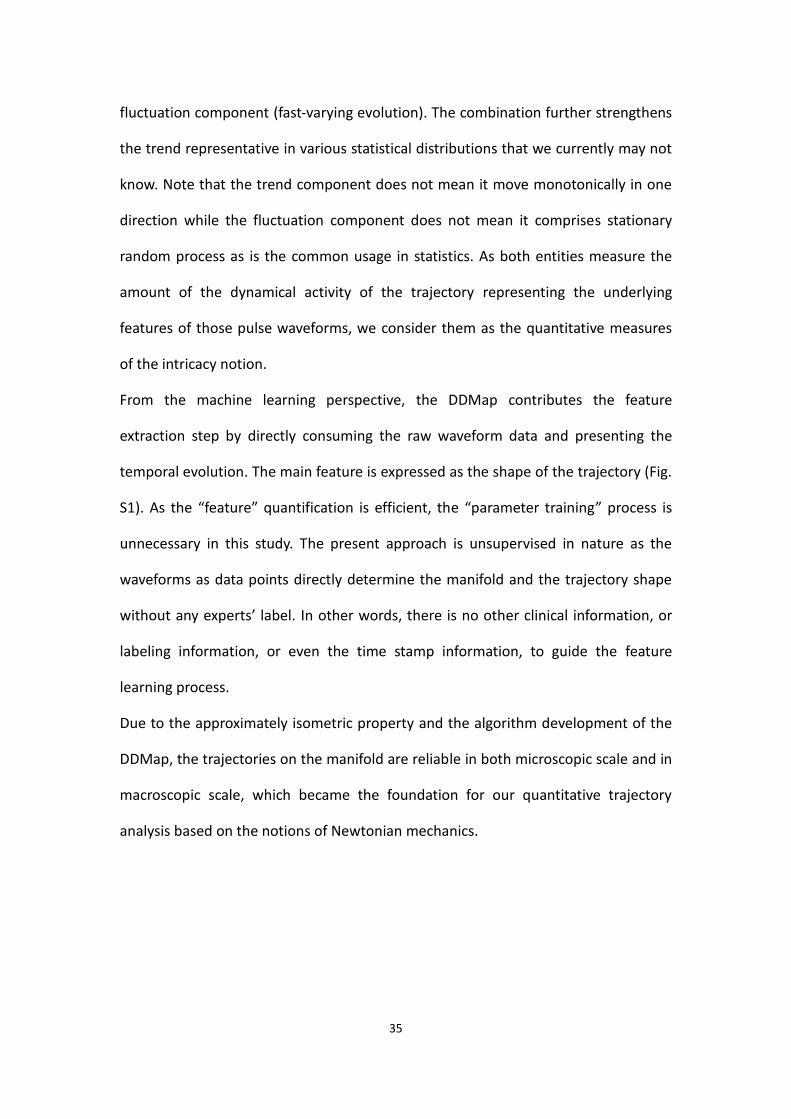
fluctuation component (fast-varying evolution). The combination further strengthens
the trend representative in various statistical distributions that we currently may not
know. Note that the trend component does not mean it move monotonically in one
direction while the fluctuation component does not mean it comprises stationary
random process as is the common usage in statistics. As both entities measure the
amount of the dynamical activity of the trajectory representing the underlying
features of those pulse waveforms, we consider them as the quantitative measures
of the intricacy notion.
From the machine learning perspective, the DDMap contributes the feature
extraction step by directly consuming the raw waveform data and presenting the
temporal evolution. The main feature is expressed as the shape of the trajectory (Fig.
S1). As the “feature” quantification is efficient, the “parameter training” process is
unnecessary in this study. The present approach is unsupervised in nature as the
waveforms as data points directly determine the manifold and the trajectory shape
without any experts’ label. In other words, there is no other clinical information, or
labeling information, or even the time stamp information, to guide the feature
learning process.
Due to the approximately isometric property and the algorithm development of the
DDMap, the trajectories on the manifold are reliable in both microscopic scale and in
macroscopic scale, which became the foundation for our quantitative trajectory
analysis based on the notions of Newtonian mechanics.

36
Fig. S1. The waveform evolution is hard to be observed from the 1-minute tracing
(upper) while the 5 minutes data shows the pulse-by-pulse trajectory (middle) in
3-dimensional image via waveform analysis via manifold learning waveform analysis.
local fluctuation and its trend movement. The local fluctuation and the trend
movement (lower) further depict the trajectory shape information as quantitative
37
intricacy measures, the fluctuation movement and the trend movement.
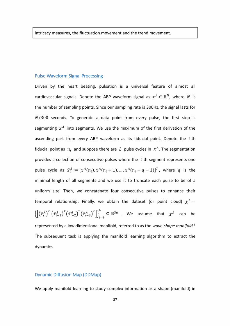
Pulse Waveform Signal Processing
Driven by the heart beating, pulsation is a universal feature of almost all
cardiovascular signals. Denote the ABP waveform signal as 𝑥𝐴 ∈ ℝ𝑁, where 𝑁 is
the number of sampling points. Since our sampling rate is 300Hz, the signal lasts for
𝑁/300 seconds. To generate a data point from every pulse, the first step is
segmenting 𝑥𝐴 into segments. We use the maximum of the first derivation of the
ascending part from every ABP waveform as its fiducial point. Denote the 𝑖-th
fiducial point as 𝑛𝑖 and suppose there are 𝐿 pulse cycles in 𝑥𝐴. The segmentation
provides a collection of consecutive pulses where the 𝑖-th segment represents one
pulse cycle as �̅�𝑖𝐴 ∶= [𝑥𝐴(𝑛𝑖), 𝑥𝐴(𝑛𝑖 + 1), … , 𝑥𝐴(𝑛𝑖 + 𝑞 − 1)]𝑇 , where 𝑞 is the
minimal length of all segments and we use it to truncate each pulse to be of a
uniform size. Then, we concatenate four consecutive pulses to enhance their
temporal relationship. Finally, we obtain the dataset (or point cloud) 𝜒𝐴 =
{[(�̅�𝑖𝐴)
𝑇 (�̅�𝑖−1
𝐴 )𝑇
(�̅�𝑖−2𝐴 )
𝑇(�̅�𝑖−3
𝐴 )𝑇
]}𝑖=3
𝐿
⊆ ℝ3𝑞 . We assume that 𝜒𝐴 can be
represented by a low dimensional manifold, referred to as the wave-shape manifold.5
The subsequent task is applying the manifold learning algorithm to extract the
dynamics.
Dynamic Diffusion Map (DDMap)
We apply manifold learning to study complex information as a shape (manifold) in

38
high dimensional space. The complex information can be summarized into a 3D
image. Dynamic Diffusion map (DDMap) is one of the manifold learning algorithms
that is a variant of diffusion map particularly designed for the ultra-long term
biomedical signal. The main reason we chose DDMap is its capability to preserve the
global structure with rigorous theoretical supports. The first step of DDMap is
preparing the point cloud 𝜒𝐴. Then, take 𝜒𝐴 to construct an 𝑛 × 𝑛 affinity matrix
𝑊 so that 𝑊𝑖𝑗 = 𝑒−|𝑥𝑖−𝑥𝑗|2/𝜀 , where 𝑖, 𝑗 = 1, … , 𝑛 and the bandwidth 𝜖 > 0 is
user defined. In practice, we set 𝜖 as the 25% percentile of all pairwise distances.
From the perspective of geometry, 𝑊𝑖𝑗 contains the information regarding
dissimilarities of all two-point pairs; the larger 𝑊𝑖𝑗 is, the more similar two points
are. Next, construct an 𝑛 × 𝑛 degree matrix 𝐷 so that 𝐷(𝑖, 𝑖) = ∑ 𝑊(𝑖, 𝑗)𝑛𝑗=1 ,
where 𝑖 = 1, … , 𝑛. Using both matrix 𝑊 and 𝐷, we obtain the transition matrix
𝐴 ≔ 𝐷−1𝑊. It depicts a random walk in the point cloud 𝜒𝐴 that integrates the
geometric structure within the data, and simultaneously suppresses the undesired
noise. The eigen-decomposition of 𝐴 = 𝑈Λ𝑉𝑇 with eigenvalues 1 = 𝜆1 > 𝜆2 ≥
𝜆3 ≥ ⋯ 𝜆𝑛 of A and 𝜙1, 𝜙2, … , 𝜙𝑛 ∈ ℝ𝑛 the corresponding eigenvectors. Finally, we
get the DDMap as Φ𝑡: 𝑥𝑗 ↦ (𝜆2𝑡 𝜙2(𝑗), 𝜆3
𝑡 𝜙3(𝑗), … , 𝜆�̂�+1𝑡 𝜙�̂�+1(𝑗)) ∈ ℝ�̂�, where 𝑗 =
1, … , 𝑛 , 𝑡 > 0 is the user-defined diffusion time, and �̂� is the user-defined
embedding dimension, and note that 𝑗 represents index of each pulse waveform.
We discard 𝜆1 and 𝜙1 as they contain no information. We empirically chose the
dimension �̂� as 15 or less as the eigenvalues decay fast enough for pulse waveform
data so that the eigenvalues of �̂� > 15 are neglectable. That is, DDMap converts a
pulse cycle to a vector that contains 15 parameters. We can then define the diffusion
distance (DDist) as the straight line distance between two points Φ𝑡(𝑥𝑖) and
Φ𝑡(𝑥𝑗) (technically, the 𝐿2 distance) as 𝐷𝑡(𝑥𝑖, 𝑥𝑗) ∶= ‖Φ𝑡(𝑥𝑖) − Φ𝑡(𝑥𝑗)‖𝑙2 . We
39
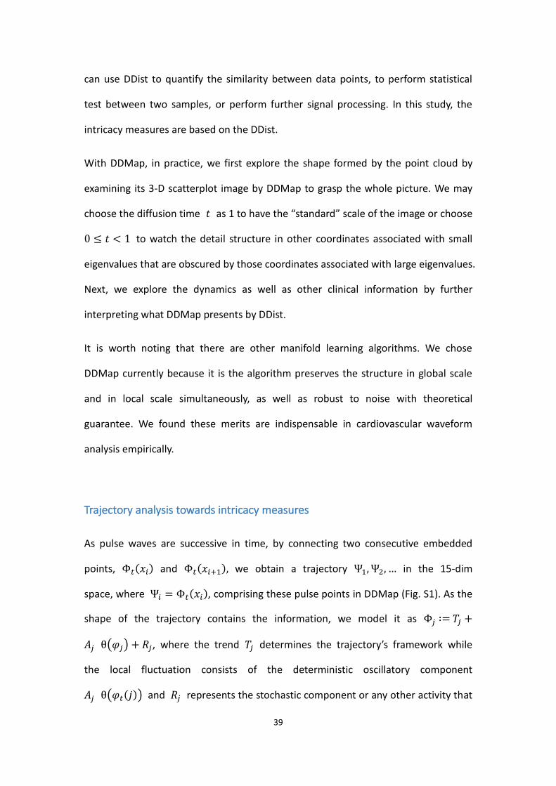
can use DDist to quantify the similarity between data points, to perform statistical
test between two samples, or perform further signal processing. In this study, the
intricacy measures are based on the DDist.
With DDMap, in practice, we first explore the shape formed by the point cloud by
examining its 3-D scatterplot image by DDMap to grasp the whole picture. We may
choose the diffusion time 𝑡 as 1 to have the “standard” scale of the image or choose
0 ≤ 𝑡 < 1 to watch the detail structure in other coordinates associated with small
eigenvalues that are obscured by those coordinates associated with large eigenvalues.
Next, we explore the dynamics as well as other clinical information by further
interpreting what DDMap presents by DDist.
It is worth noting that there are other manifold learning algorithms. We chose
DDMap currently because it is the algorithm preserves the structure in global scale
and in local scale simultaneously, as well as robust to noise with theoretical
guarantee. We found these merits are indispensable in cardiovascular waveform
analysis empirically.
Trajectory analysis towards intricacy measures
As pulse waves are successive in time, by connecting two consecutive embedded
points, Φ𝑡(𝑥𝑖) and Φ𝑡(𝑥𝑖+1), we obtain a trajectory Ψ1, Ψ2, … in the 15-dim
space, where Ψ𝑖 = Φ𝑡(𝑥𝑖), comprising these pulse points in DDMap (Fig. S1). As the
shape of the trajectory contains the information, we model it as Φ𝑗 ∶= 𝑇𝑗 +
𝐴𝑗 θ(𝜑𝑗) + 𝑅𝑗, where the trend 𝑇𝑗 determines the trajectory’s framework while
the local fluctuation consists of the deterministic oscillatory component
𝐴𝑗 θ(𝜑𝑡(𝑗)) and 𝑅𝑗 represents the stochastic component or any other activity that

40
cannot be represented by oscillatory activity. The oscillatory component is supposed
to be a 1-periodic function θ with mean 0 attached with the amplitude 𝐴𝑗 and
phase 𝜑𝑗. Based on this model, we applied a moving median followed by a moving
mean filter to extract the trend, 𝑇�̂�: =1
𝑘∑ 𝑀𝑒𝑑𝑖𝑎𝑛(Ψ𝑚
, Ψ𝑚−1 , … , Ψ𝑚−𝑘+1
)𝑗𝑚=𝑗−𝑘+1 ,
where both filters are parameterized by the size 𝑘. Then we have the fluctuation
term 𝐴𝑗 θ(𝜑𝑡(𝑗)) + 𝑅𝑗 = Φ𝑗 − 𝑇�̂�. In this study, we do not further decompose the
fluctuation term into 𝐴𝑗 θ(𝜑𝑡(𝑗)) and 𝑅𝑗 in the above model, as we focus on
observing how the trend and non-trend behave in the real world data. The
“pulse-wise” fluctuation movement is calculated as the Euclidean distance between
the trajectory and the trend as ‖Φ𝑗 − 𝑇�̂�‖
𝑙2. Note that if 𝑇�̂� = Φ𝑚 for some 𝑚,
‖Φ𝑗 − 𝑇�̂�‖
𝑙2 is the DDist between Φ𝑗 and 𝑇�̂�. In this study we use its mean value to
represent one intricacy measure within a period.
Another intricacy index, the trend movement, is calculated as the length of the
piecewise trajectory path per second as (∑ ‖�̂�𝑖 − �̂�𝑖−1‖𝐿𝑖=1 𝑙 2) 𝑇⁄ for a signal of 𝑇
seconds containing 𝐿 pulses. We borrow the notion of speed to make this intricacy
measure quantify how fast the trend evolving. In summary, both intricacy measures,
the trend movement and fluctuation movement, are intuitively derived from the
trajectory structure to measure the amount of waveform dynamics.
For the convenience of future clinical application, both indices would be better to be
represented in a roughly 0-100 range. Therefore, we pool all ABP data segments
(presurgical: 60 cases, anhepatic: 57 cases, neohepatic phase: 58 cases) and
employed the formula as follows to remap. The trend movement is calculated as
𝑟𝑜𝑤 𝑡𝑟𝑒𝑛𝑑 𝑚𝑜𝑣𝑒𝑚𝑒𝑛𝑡−𝑚𝑒𝑑𝑖𝑎𝑛(𝑝𝑜𝑜𝑙𝑒𝑑 𝑟𝑜𝑤 𝑡𝑟𝑒𝑛𝑑 𝑚𝑜𝑣𝑒𝑚𝑒𝑛𝑡𝑠)
𝐼𝑄𝑅(𝑝𝑜𝑜𝑙𝑒𝑑 𝑟𝑜𝑤 𝑡𝑟𝑒𝑛𝑑 𝑚𝑜𝑣𝑒𝑚𝑒𝑛𝑡𝑠)× 25 + 60. So is the fluctuation

41
movement. As both median and IQR are calculated with the quantile function, of
which the algorithm has several versions in history and produces slightly different
values, we standardized it as the type 8 algorithm according to the recommendation
of the R documentation.
Calculation of MELD score and Early Allograft Failure Scores
Taking care of liver recipients requires intense medical resources and teamwork
dedication. From the intraoperative anesthetic management to post-operative
follow-up, sometimes the decision making is challenging based on enormous clinical
data accumulated over time. Effective data interpretation generates valuable
information. While statistical methods require adequate sample size to perform
hypothesis tests, introducing new technologies to assess data obtained from each
liver recipient may also reveal clinical details.
The MELD and EAF scores, including model for early allograft function (MEAF) score,
Early Allograft Failure Simplified Estimation (EASE) score, and the liver graft
assessment following transplantation (L-GrAFT7) risk score, were developed based
on the laboratory data from a large number of cases to assess the general condition
of the liver transplant recipient. As the disease acuity may also compromise
numerous physiological mechanisms for homeosis, we propose that the ABP
waveforms evolving with time reflect the severity of the patient’s condition, and
these scores allow us to investigate the ABP waveform evolution structure with
respect to the conditions immediately before the surgery and afterward.
Below we detail these scores. We calculated them according to the formula reported
in the corresponding literature and validated by materials provided by the
corresponding authors through private communication.
The MEAF score is derived from three laboratory data, ALT, INR, and Bilirubin, within
3 postoperative days. The MEAF score is calculated as:
𝑀𝐸𝐴𝐹 = (3.29 (1 + 𝑒−1.9132(ln(𝐴𝐿𝑇𝑚𝑎𝑥.3𝑝𝑜𝑑)−6.1723))⁄ )
+ (3.29 (1 + 𝑒−6.8204(ln(𝐼𝑁𝑅𝑚𝑎𝑥.3𝑝𝑜𝑑)−0.6658)⁄ )
+ (3.29 (1 + 𝑒−1.8005(ln(𝑏𝑖𝑙𝑖𝑟𝑢𝑏𝑖𝑛3𝑝𝑜𝑑)−1.0607)⁄ )
42
The L-GrAFT7 score and L-GrAFT10 score comprise the laboratory data of AST, INR,
total bilirubin, and platelet counts at day 7 and day 10 respectively. We compute
L-GrAFT7 as
6.96470 − 0.57990 × ∑ ln 𝐴𝑆𝑇𝑑𝑎𝑦 + 0.00844 × (∑ ln 𝐴𝑆𝑇𝑑𝑎𝑦7𝑑𝑎𝑦=1 )7
𝑑𝑎𝑦=1
2+
5.25347 × 𝑆𝑙𝑜𝑝𝑒 (ln 𝐴𝑆𝑇𝑑𝑎𝑦1 , … ln 𝐴𝑆𝑇𝑑𝑎𝑦7) + 4.65046 ×
𝑆𝑙𝑜𝑝𝑒 (ln 𝐴𝑆𝑇𝑑𝑎𝑦1 , … ln 𝐴𝑆𝑇𝑑𝑎𝑦7)2
+ 1.14098 × ∑ ln 𝐼𝑁𝑅𝑑𝑎𝑦7𝑑𝑎𝑦=1 −
0.03475 × ∑ ln 𝑇𝐵𝐼𝐿𝑑𝑎𝑦7𝑑𝑎𝑦=1 + 0.00562 × (∑ ln 𝑇𝐵𝐼𝐿𝑑𝑎𝑦
7𝑑𝑎𝑦=1 ) 2 +
4.31135 × 𝑆𝐿𝑂𝑃𝐸(ln 𝑇𝐵𝐼𝐿𝑑𝑎𝑦1 , … ln 𝑇𝐵𝐼𝐿𝑑𝑎𝑦7) + 5.84724 ×
𝑆𝐿𝑂𝑃𝐸(ln 𝑇𝐵𝐼𝐿𝑑𝑎𝑦1 , … ln 𝑇𝐵𝐼𝐿𝑑𝑎𝑦7)2
− 0.05115 × ∑ ln 𝑃𝐿𝑇𝑑𝑎𝑦7𝑑𝑎𝑦=1 ,
where 𝑙𝑛 represents the natural logarithmic function, and L-GrAFT10 is calculated
as
9.77 − 0.42946 × ∑ log(𝐴𝑆𝑇𝑑𝑎𝑦)10𝑑𝑎𝑦=1 + 0.00462 ×
(∑ log(𝐴𝑆𝑇𝑑𝑎𝑦))10𝑑𝑎𝑦=1
2+ 4.60719 × 𝑆𝑙𝑜𝑝𝑒 (ln 𝐴𝑆𝑇𝑑𝑎𝑦1 , … ln 𝐴𝑆𝑇𝑑𝑎𝑦7) +
4.4129 × 𝑆𝑙𝑜𝑝𝑒 (ln 𝐴𝑆𝑇𝑑𝑎𝑦1 , … ln 𝐴𝑆𝑇𝑑𝑎𝑦7)2
+ 0.88974 ×
𝑀𝐴𝑋(ln 𝐼𝑁𝑅𝑑𝑎𝑦1 , … , ln 𝐼𝑁𝑅𝑑𝑎𝑦10) − 0.04852 × ∑ ln 𝑇𝐵𝐼𝐿𝑑𝑎𝑦10𝑑𝑎𝑦=1 +
0.00363 × (∑ ln 𝑇𝐵𝐼𝐿𝑑𝑎𝑦10𝑑𝑎𝑦=1 ) 2 + 5.33627 ×
𝑆𝐿𝑂𝑃𝐸(ln 𝑇𝐵𝐼𝐿𝑑𝑎𝑦1 , … ln 𝑇𝐵𝐼𝐿𝑑𝑎𝑦10) − 0.04621 × ∑ ln 𝑃𝐿𝑇𝑑𝑎𝑦10𝑑𝑎𝑦=1 −
5.24897 × 𝑆𝐿𝑂𝑃𝐸(ln 𝑃𝐿𝑇𝑑𝑎𝑦1 , … ln 𝑃𝐿𝑇𝑑𝑎𝑦10) + 13.08633 ×
𝑆𝐿𝑂𝑃𝐸(ln 𝑃𝐿𝑇𝑑𝑎𝑦1 , … ln 𝑃𝐿𝑇𝑑𝑎𝑦10)2.
In comparison with the above scores, the EASE score consumes more items,
including the laboratory data of AST, platelet, bilirubin within 10 days, the MELD
score, the number of transfused packed red bleed cell during surgery, the events of
vascular thrombosis within 10 days after the surgery and whether the early volume
of the institution is larger than 70 cases per year. It is calculated as
0.000534 ×
𝐴𝑈𝐶(ln 𝐴𝑆𝑇𝑑𝑎𝑦1 , ln 𝐴𝑆𝑇𝑑𝑎𝑦2 , ln 𝐴𝑆𝑇𝑑𝑎𝑦3 , ln 𝐴𝑆𝑇𝑑𝑎𝑦7 , ln 𝐴𝑆𝑇𝑑𝑎𝑦10) −
0.093 × 𝐴𝑈𝐶(ln 𝑃𝐿𝑇𝑑𝑎𝑦1 , ln 𝑃𝐿𝑇𝑑𝑎𝑦3 , ln 𝑃𝐿𝑇𝑑𝑎𝑦7 , ln 𝑃𝐿𝑇𝑑𝑎𝑦10) − 7.766 ×
𝑆𝐿𝑂𝑃𝐸(ln 𝑃𝐿𝑇𝑑𝑎𝑦1 , ln 𝑃𝐿𝑇𝑑𝑎𝑦3 , ln 𝑃𝐿𝑇𝑑𝑎𝑦7 , ln 𝑃𝐿𝑇𝑑𝑎𝑦10) + 0.795 ×
43
𝑆𝐿𝑂𝑃𝐸(ln 𝑇𝐵𝐼𝐿𝑑𝑎𝑦1 , ln 𝑇𝐵𝐼𝐿𝑑𝑎𝑦3 , ln 𝑇𝐵𝐼𝐿𝑑𝑎𝑦7 , ln 𝑇𝐵𝐼𝐿𝑑𝑎𝑦10) + 0.044 ×
𝑀𝐸𝐿𝐷 + 0.065 × 𝑃𝑅𝐵𝐶 + 2.567 × 𝑡ℎ𝑟𝑜𝑚𝑏𝑜𝑠𝑖𝑠 − 0.402 × 𝑣𝑜𝑙𝑢𝑚𝑒 − 0.602,
where 𝐴𝑈𝐶 represents the area under the curve evaluated by the trapezoid sum,
𝑡ℎ𝑟𝑜𝑚𝑏𝑜𝑠𝑖𝑠 is 1 if arterial or portal thrombosis taken place within 10 days
postoperatively and 0 otherwise, and 𝑣𝑜𝑙𝑢𝑚𝑒 is 1 if the institutional case volume
more than or equal to 70 cases per year and 0 otherwise.
Supplementary Results
Sensitivity analysis of MELD score correlations
In this sensitivity analysis, we test the effect of filter size parameter K, which
determines the time scale of both intricacy indices, the fluctuation movement and
trend movement. The goal is to confirm if the quantitative indices are sensitive to the
chosen parameters/model or not, and how them affect the performance in reflecting
the dynamical surgical phases transition from the presurgical phase to anhepatic
phase.
For the Pearson correlation between presurgical ABP data and the MELD score (Fig
S2), the trend movements achieve statistical significance from all K (K=8 to 140)
whereas the fluctuation movements become significant from K=18. The trend
movement reaches maximum correlation at K=40 while the fluctuation movement at
K=130. Both indices show smooth curves in their correlations, indicating the
robustness over the K parameter. For quantifying the smoothness of the curve, all
the differences between adjacent correlation coefficients are small for the
correlations between MELD and the presurgical fluctuation movement (-0.013
[-0.026, -0.006, IQR=0.020]), the correlations between MELD-Na and the presurgical
fluctuation movement (-0.014 [-0.025, -0.007, IQR=0.017]), the correlations between
44
MELD and the presurgical trend movement (0.0029 [-0.0029, 0.009, IQR=0.012]), and
the correlations between MELD-Na and the presurgical trend movement (0.0019
[-0.0029, 0.009, IQR=0.012]),
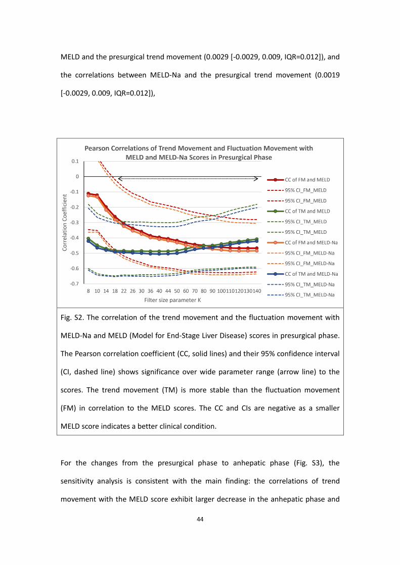
Fig. S2. The correlation of the trend movement and the fluctuation movement with
MELD-Na and MELD (Model for End-Stage Liver Disease) scores in presurgical phase.
The Pearson correlation coefficient (CC, solid lines) and their 95% confidence interval
(CI, dashed line) shows significance over wide parameter range (arrow line) to the
scores. The trend movement (TM) is more stable than the fluctuation movement
(FM) in correlation to the MELD scores. The CC and CIs are negative as a smaller
MELD score indicates a better clinical condition.
For the changes from the presurgical phase to anhepatic phase (Fig. S3), the
sensitivity analysis is consistent with the main finding: the correlations of trend
movement with the MELD score exhibit larger decrease in the anhepatic phase and

45
no recovery in the neohepatic phase, whereas the correlations of fluctuation
movement are relatively maintained. The chosen parameter K=90 presents the
largest drop of the correlation with the MELD and MELD-Na scores, while other K
also presents a large drop, which suggests the robustness of both trend movement
and fluctuation movement with regard to the choice of K. The smooth curves also
present the robustness of both indices. We conclude from this sensitivity analysis
that the derivation of the ABP intricacy indices would help reveal the temporal
evolution structure in ABP data.

46
Fig. S3. The drop of the MELD correlations (upper panel) from the presurgical (dotted
line) to anhepatic phase (solid line) with trend movement (TM) are larger than that
with fluctuation movement (FM). For the drop of the correlation of TM (lower panel),
parameter K=90 represents the most dynamical change from the presurgical to
anhepatic phase. The arrow indicates the largest decrease at K=90. The smooth
correlation coefficient curves indicate the numeric robustness of both FM and TM
indices.
Null Model Test
In this null model validation test (Fig. S4), we first replace waveform by mean blood
pressure to replace waveform and evaluate the correlation with the MELD scores. For
the presurgical phase, compared with the fluctuation movement, the correlation is
decreased (MELD-Na: -0.450 → -0.380, MELD: -0.436 → -0.374), so is the presurgical
trend movement (MELD-Na: -0.480 → -0.405, MELD: -0.468 → -0.395). Both
maintain statistical significance.
The second null model validation test is the surrogate data test by randomly
permuting the time sequence of the ABP pulses. It shows the decreases of
correlation for the fluctuation movement (MELD-Na: -0.450 → -0.389, MELD: -0.436
→ -0.376) and trend movement (MELD-Na: -0.480 → -0.247, MELD: -0.468 → -0.234).
The trend movement shows a larger drop in the correlation than the fluctuation
movement. Both maintain statistical significance.
The third null model validation test is permuting case labeling; that is, random pair
MELD scores and ABP waveforms. It shows no correlation in both indices. The loss of
association justifies our hypothesis between ABP intricacy and recipient’s acuity
condition.

47
Fig. S4. The null model validation tests of the Pearson’s correlations between MELD
scores and the intricacy indices in the presurgical phase with the error bars indicating
95% confidence intervals. By removing waveform information with mean blood
pressure, the attenuated associations still show significance, suggesting the
contribution of the blood pressure value. By removing the time sequence
information between successive pulses, the attenuated associations, suggesting the
contribution of variance information. By removing the case MELD score association,
the loss of association justifies our hypothesis between ABP intricacy and the acuity
condition.