DISCOVER: Keyword Search in Relational Databases

Vagelis HristidisUniversity of California, San Diego

vagelis@cs.ucsd.edu

Yannis PapakonstantinouUniversity of California, San Diego

yannis@cs.ucsd.edu

Abstract

DISCOVER operates on relational databases andfacilitates information discovery on them by al-lowing its user to issue keyword queries withoutany knowledge of the database schema or of SQL.DISCOVER returns qualified joining networks oftuples, that is, sets of tuples that are associated be-cause they join on their primary and foreign keysand collectively contain all the keywords of thequery. DISCOVER proceeds in two steps. Firstthe Candidate Network Generator generates allcandidate networks of relations, that is, join ex-pressions that generate the joining networks of tu-ples. Then the Plan Generator builds plans forthe efficient evaluation of the set of candidate net-works, exploiting the opportunities to reuse com-mon subexpressions of the candidate networks.

We prove that DISCOVER finds without redun-dancy all relevant candidate networks, whose sizecan be data bound, by exploiting the structure ofthe schema. We prove that the selection of theoptimal execution plan (way to reuse commonsubexpressions) is NP-complete. We provide agreedy algorithm and we show that it providesnear-optimal plan execution time cost. Our ex-perimentation also provides hints on tuning thegreedy algorithm.

1 Introduction

Keyword search is the most popular information discov-ery method because the user does not need to know eithera query language or the underlying structure of the data.The search engines available today provide keyword searchon top of sets of documents. When a set of keywords is

Permission to copy without fee all or part of this material is granted pro-vided that the copies are not made or distributed for direct commercialadvantage, the VLDB copyright notice and the title of the publication andits date appear, and notice is given that copying is by permission of theVery Large Data Base Endowment. To copy otherwise, or to republish,requires a fee and/or special permission from the Endowment.

Proceedings of the 28th VLDB Conference,Hong Kong, China, 2002

provided by the user, the search engine returns all docu-ments that are associated with these keywords. Typically,two keywords and a document are associated when the key-words are contained in the document and their degree ofassociativity is often their distance from each other.

In addition to documents, a huge amount of informationis stored in relational databases, but information discov-ery on relational databases is not well supported. The userof a relational database needs to know the schema of thedatabase, SQL or some QBE-like interface, and the rolesof the various entities and terms used in the query. Theuser of DISCOVER does not need knowledge of any of theabove. Instead, DISCOVER enables information discoveryby providing a straightforward keyword search interface tothe database.

For example, consider the TPC-H schema shown in Fig-ure 1 and the instance in Figure 2. The arrows in Figure 1point in the direction of the primary to foreign key (one-to-many) relationships between tables. Consider a usersearching for information on the association of the key-words “Smith” and “Miller”. DISCOVER provides a sim-ple interface where the user simply types the keywords – ashe would do on a search engine. According to DISCOVER,an association exists between two keywords if they are con-tained in two associated tuples, i.e., two tuples that jointhrough foreign key to primary key relationships, whichpotentially involve more tuples. This form of association isparticularly useful and challenging. (We comment on otherassociation criteria at the end.) DISCOVER does not re-quire from the user to know the relations and the attributeswhere the keywords are found.

The solution to the query are the two minimal joiningsequences that contain the keywords “Smith” and “Miller”,namely o1 �� c1 �� o2 and o1 �� c1 �� n1 �� c2 �� o3. Theyare minimal in the sense that no tuple can be excluded andstill have a sequence that contains the keywords. We usethe notation a �� b to denote that tuple a joins with tuple bon their primary key to foreign key relationship. The firstjoining sequence shows that both “Smith” and “Miller” areclerks that have served customer Brad Lou, whereas thesecond merely says that the clerks have served customersBrad Lou and George Walters respectively, who both comefrom the USA. Intuitively, the first joining sequence is moreuseful than the second because it shows a closer association

Figure 1: The TPC-H schema (copied from www.tpc.org)

Figure 2: Sample TPC-H database instance

between “Smith” and “Miller”. Based on the generaliza-tion of this intuition we rank join sequences according tothe number of joins they involve. DISCOVER outputs theshorter sequences first.

When more than two keywords are involved, a mini-mal joining sequence may not be sufficient to represent asolution. Hence we introduce minimal joining networks,that are trees of tuples where any two adjacent tuples jointhrough a primary key to foreign key relationship.

A high level representation of the architecture DIS-COVER uses to find the joining networks is shown in Fig-ure 3. First, the user gives a set of keywords k1� � � � �km tothe system. These keywords are looked up in the master in-dex, which returns the tuple sets Rk1

i � � � � �Rkmi for each rela-

tion Ri. Every tuple of Rkji contains keyword k j as part of an

attribute value. Then DISCOVER calculates all candidatenetworks, i.e., join expressions on foreign to primary keyrelationships of relations or tuple sets, as shown in Figure 3.The set of candidate networks is guaranteed to produce all

Keywords "Smith","Miller"

Master Index

Basic Tuple Sets

Tuple SetPost-Processor

Tuple Sets

Candidate NetworkGenerator

DatabaseSchema

Plan Generator

Plan Execution

Database

Candidate Networks

Execution Plan

SQL queries

CREATE TABLE T1 AS SELECT * FROMORDERSSmith, CUSTOMERS WHERE ...

SELECT * FROM T1, ORDERSMiller WHERE ...SELECT * FROM T1, NATION, CUSTOMERS,

ORDERSMiller WHERE ...

Joining Networks oftuples

User

ORDERSSmith={o1}ORDERSMiller={o2,o3}

Figure 3: Architecture of DISCOVER

the minimal joining networks.Then DISCOVER evaluates the candidate networks.

Due to the nature of the problem, the candidate networksshare join expressions. This offers an opportunity to builda set of intermediate results and use them in the computa-tion of multiple candidate networks. The Plan Generatorproduces an execution plan that calculates and uses inter-mediate results in evaluating the candidate networks. Fi-nally an SQL statement is produced for each line of the ex-ecution plan and these statements are passed to the DBMS.The DBMS returns the joining networks of tuples that arethe solutions to the problem.

Notice that the candidate networks may have a numberof joins that is only bound by the dataset as it is explainedlater. In these cases the user supplies a maximum numberT of joins and DISCOVER incrementally outputs all can-didate networks up to size T .

The challenges involved in the above process and thecontributions of this paper are the following:� We formalize keyword search on relational databases

and provide intuitive semantics.� We propose a modular architecture and have imple-

mented DISCOVER based on it.� We present an efficient candidate network generation

algorithm. The naive approach would be to gen-erate all join expressions up to size T that containall keywords and then evaluate them. However, weprune out many of them by exploiting the propertiesof the schema of the database and the information re-turned by the master index. For example in the key-word query “Smith, Miller”, the candidate networkORDERSSmith �� CUSTOMER�� �� ORDERSMiller ��

LINEIT EM�� is pruned out because LINEIT EM��

has no keywords and since it is in the end of the join-ing sequence’s chain, it cannot help in joining anytuple that could lead to a keyword. For more com-plex reasons, pertaining to the structure of the pri-mary key to foreign key relationships as discussedlater, candidate networks such as ORDERSSmith ��

LINEIT EM�� �� ORDERSMiller are also excluded.� We prove that the candidate network generation al-

gorithm creates a complete and non-redundant set ofcandidate networks, where “complete” means that theset of candidate networks produces all minimal join-ing networks of tuples (up to a given size T ) and “non-redundant” means that if any candidate network of theset is excluded then there are database instances wherethere are minimal joining networks of tuples that arenot discovered. It is also shown that the results of thecandidate networks are always minimal joining net-works of tuples.

� We specify when the maximum size of the candi-date networks is bound by the size of the databaseschema and when it is bound only by the size of thedatabase instance. For the former case, we providetheorems that specify the maximum size Tmax of theminimal joining networks of tuples, as a function ofthe database schema.

� We propose a cost model. The Plan Generator moduleuses intermediate results to minimize the total cost ofthe evaluation of all candidate networks. We show thatthe problem of selecting the optimal set of intermedi-ate results is NP-complete on the size of the candidatenetworks. We then present a tunable greedy algorithmthat discovers near-optimal plans, without sufferingfrom the unacceptable optimization time cost incurredby the optimal planning algorithm.

� DISCOVER has been implemented on top of Oracle8i. We present a detailed experimental evaluation ofthe modules of DISCOVER and of the overall sys-tem. It is shown that a large percentage of the gen-erated candidate networks are pruned. Furthermore,we show how to tune the greedy algorithm to achievethe best possible performance and we show that theoverall performance beats by far the performance ofthe obvious straightforward approaches.

In Section 2 we compare DISCOVER to other relatedefforts. Sections 4 and 5 present the Candidate NetworkGenerator and the Plan Generator module respectively. InSection 6 we evaluate experimentally the performance ofDISCOVER. Finally, in Section 7 we conclude and discussfuture extensions and improvements of DISCOVER.

2 Related WorkA framework for keyword search on databases when theschema is not known to the user is presented in [MV00b,MV00a]. An extension of SQL called Reflective SQL(RSQL) is introduced, which treats data and queries uni-formly. The main limitation of this work is that all key-words must be contained in the same tuple. That is, the re-

lationships between tuples from different relations are nottaken into consideration.

In [GSVGM98] and [BNH�02], a database is viewedas a graph with objects/tuples as nodes and relationshipsas edges. Relationships are defined based on the proper-ties of each application. For example an edge may denotea primary to foreign key relationship. In [GSVGM98], theuser query specifies two sets of objects, the Find and theNear objects. These objects may be generated from twocorresponding sets of keywords. The system ranks the ob-jects in Find according to their distance from the objects inNear. An algorithm is presented that efficiently calculatesthese distances by building hub indices. In [BNH�02], an-swers to keyword queries are provided by searching forSteiner trees [Ple81] that contain all keywords. Heuris-tics are used to approximate the Steiner tree problem. Adrawback of these approaches is that a graph of the tuplesmust be created and maintained for the database. Further-more, the important structural information provided by thedatabase schema is ignored and their algorithms work onhuge data graphs. In contrast, DISCOVER is tuned to key-word search on relational databases and uses the propertiesof the schema of the database. Its key algorithms workon the schema graph, which is much smaller than the datagraph, and does not need to keep any extra data represen-tations. It exploits the properties of the database schemato produce the minimum number of SQL queries neededto answer to the keyword query. Furthermore, DISCOVERoperates directly on the databases, so it does not have amain memory space limitation.

The work of the Candidate Network Generator remindsof algorithms for answering queries on universal relations[Ull82]. However there are many important differences be-tween universal relations and DISCOVER: First, there isthe obvious difference that the user of a Universal Relation(UR) needs to know the attributes where the keywords are,in contrast to the user of DISCOVER. Second, DISCOVERcreates efficient queries that find all connections betweenthe tuples that contain the keywords. In doing so, DIS-COVER, unlike the UR, has to find connections whose sizemay not be schema bound and many of them are prunedby DISCOVER’s Candidate Network Generator. Finally,in addition to finding the useful connections, DISCOVERexploits the fact that the connections are “correlated”, inthe sense that they share join expressions. This leads to aspecial query optimization algorithm, which is tuned to thespecifics of our problem.

DBXplorer [ACD02] describes a multi-step system toanswer keyword queries in relational databases and freesthe user from the first limitation of the universal relations.However it does not consider solutions that include two tu-ples from the same relation. Furthermore they only con-sider exact matches, where a keyword must match exactlyan attribute value and they do not exploit the reusabilityopportunities of the join trees, which is a simplified notionclose to the candidate networks of DISCOVER.

Oracle 9i Text ([Ora01]) and IBM DB2 Text Informa-

tion Extender ([DB201]) use standard SQL to create fulltext indices on text attributes of relations. Microsoft SQLServer 2000 ([MSD01]) also provides tools to generate fulltext indices, which are stored in files outside the database.In all three systems, the user creates full text indices onsingle attributes and then performs keyword queries, whichreturn the tuples that contain a keyword. Furthermore, key-word proximity queries are supported within a single at-tribute of a tuple, but not across different attributes or tu-ples. As we discuss, generalizing keyword search to workacross tuples is very challenging and the issues are differentfrom the text indexing issues that those systems address.

One of the criteria that we use to decide that a join ex-pression J is not a candidate network is whether the joiningnetworks of tuples produced by J contain more than one oc-currences of the same tuple. Our approach for deciding thisproperty can be viewed as a special case of the chase tech-nique with inclusion dependencies presented in [AHV95].Our algorithm is simpler, faster and decidable, since it fo-cuses on primary to foreign key relationships.

Keyword search has been well studied for documentdatabases ([Sal89]). For example [BP98] presents theGoogle search engine. [ACGM�01] offers an overviewof current Web search engine design. It also introduces ageneric search engine architecture and covers crawling andindexing issues. In [TWW�00], algorithms , data struc-tures, and software are presented that approach the speedof keyword-based document search engines for querieson structural databases like parse trees, molecular dia-grams and XML documents. [FKM99] tackles the keywordsearch problem in XML databases. They propose an exten-sion to XML query languages that enables keyword searchat the granularity of XML elements, which helps noviceusers formulate queries, but do not consider keyword prox-imity search.

The use of common subexpressions by the Plan Gener-ator is a form of multi-query optimization [Sel88, Fin82,RSSB00]. However the candidate networks in DISCOVERhave special properties that allow us to develop a morestraightforward and efficient algorithm. The first propertyis that the candidate networks have small relations [Ull82]as leaves, which dramatically prunes the space of usefulcommon subexpressions when applying the Wong-Yusefialgorithm [Ull82]. Second, the candidate networks are notrandom queries, but share common subexpressions by thenature of their generation as we see in Section 4. The tech-niques of [Fin82] cannot be applied to DISCOVER sincethey concentrate on finding common subexpressions as apost-phase to query optimization and DISCOVER does nothave access to the DBMS optimizer.

3 Framework

3.1 Data Model and Keyword Queries

We consider a database that has n relations R1� � � � �Rn. Eachrelation Ri has mi attributes ai

1� � � � �aimi

. The schema graphG is a directed graph that captures the primary key to for-

eign key relationships in the database schema. It has a nodeRi for each relation Ri of the database and an edge Ri � R jfor each primary key to foreign key relationship from aset of attributes �ai

b1� � � � �ai

bl� of Ri to a set of attributes

�a jb1� � � � �a j

bl� of R j, where ai

bk� a j

bkfor k � 1� � � � � l. We

define the graph Gu to be the undirected version of G.For notational simplicity, we assume that the attributes

of a primary to foreign key relationship have the same nameand that there are no self loops or parallel edges in theschema graph. So an edge Ri � R j uniquely identifies thecorresponding primary and foreign key attributes. We alsoassume that no set of attributes of any relation is both a pri-mary key and a foreign key for two other relations, which isa reasonable assumption for any realistic database schemadesign. The generalization of the problem and the solutionwhen these assumptions do not hold is trivial.

We denote the primary key of a tuple t � R as p�t� andits foreign key that references relation S as f S�t�.

Definition 1 (Joining network of tuples) A joining net-work of tuples j is a tree of tuples where for each pair ofadjacent tuples ti� t j � j, where ti � Ri� t j � R j, there is anedge �Ri�R j� in Gu and �t i �� t j� � �Ri �� R j�.

The size of a joining network is the number of joins that itinvolves, which is one less than the tree’s size. An exam-ple of a joining network of tuples in Figure 2 is

c1

n1o2o1,

which can be written in line notation as c1�o1�o2�n1� oro1�c1�o2�n1��. Its size is 3.

A joining sequence of tuples is a special case of a join-ing network of tuples, where each internal node of the treehas exactly two adjacent nodes. An example of a joiningsequence of tuples in Figure 2 is c1�o1�o2�, also denoted aso1 �� c1 �� o2.

Definition 2 (Keyword Query) A keyword query is a setof keywords k1� � � � �km. The result of the keyword query isthe set of all possible joining networks of tuples that areboth:� Total: every keyword is contained in at least one tuple

of the joining network.� Minimal: we can not remove any tuple from the join-

ing network and still have a total joining network oftuples.

We call such joining networks Minimal Total Joining Net-works of Tuples (MTJNT) of the keywords k1� � � � �km orsimply MTJNT’s when the corresponding set of keywordsis obvious from the context.

It is obvious from the definition that the result of a keywordquery is unique. A keyword query may also be given themaximum size T of the result MT JNT ’s.

The answers to keyword queries with two keywords arealways joining sequences of tuples. On the other hand,when we have more than two keywords then the answermost often cannot be expressed as a joining sequence, sowe need a joining network. Consider for example the key-word query “Smith, Miller, USA”. The best (smallest) an-swer to this query is MT JNT c1�o1�o2�n1�.

Q

S

R

A CR B DSA BQ

a1 c1

a2 c2

a3 c3

...

an cn

a1 b1

a2 b1

a2 b2

a3 b2

a3 b3

...

an bn-1

an bn

b1 d1

b2 d2

b3 d3

...

bn dn

(a) (b)

r1

r2

r3

...

rn

q1

q2

q3

q4

q5

...

q2n-2

q2n-1

s1

s2

s3

...

sn

Figure 4: A many-to-many relationship

If there is a many-to-many relationship between two re-lations of a database, then the MT JNT ’s could have an ar-bitrarily big size, which is only data bound. Figure 4 showsan extreme case where there is a many-to-many relation-ship between two relations R�S. There is a foreign to pri-mary key relationship from Q to R and from Q to S on thehomonymous attributes. Suppose that attribute values c 1and dn contain the two keywords of a query. The MT JNTr1 �� q1 �� s1 �� q2 �� r2 �� � � � �� rk �� q2k�1 �� sk �� q2k ��

� � � �� rn �� q2n�1 �� sn uses all tuples from all three rela-tions, as shown by the arrows in Figure 4. So we see thatthe size of the joining sequence can only be bound by thedataset when there are many-to-many relationships.

Keep in mind that a keyword may be in more than onetuples of the same relation or in different relations. An ex-ample of the first case is the “Miller” keyword that appearsin two tuples (o2 and o3) of the ORDERS relation. Forthe second case, consider the keyword query “John, USA”,where the keyword “John” is contained in both tuples o 1and c3. Two joining sequences for this keyword query arec3 �� n1 and o1 �� c1 �� n1. Notice that the joining sequencesin the result in this case are heterogeneous.

3.2 Architecture

In this section we walk through the components of DIS-COVER (see Figure 3) and formally define the structure oftheir inputs and outputs. The Master Index inputs a set ofkeywords k1� � � � �km and outputs a set of basic tuple sets

R̄k ji for i � 1� � � � �n and j � 1� � � � �m. The basic tuple set

R̄k ji consists of all tuples of relation Ri that contain the key-

word k j. The master index has been implemented using theOracle8i interMedia Text 8.1.5 extension, which builds fulltext indices on single attributes of relations. Then the mas-ter index inspects the index of each attribute and combinesthe results. 1

Then the Tuple Set Post-Processor takes the basic tu-ple sets and produces tuple sets RK

i for all subsets K of

1We are currently building from scratch a more efficient master indexusing an inverted index that has one entry for each keyword k and theentry has references to all tuples that contain k. However, the master indexchoice does not affect the key challenges and tradeoffs discussed in thispaper.

�k1� � � � �km�, where

RKi � �t�t � Ri�k � K� t contains k�

k � �k1� � � � �km�K� t does not contain k� (1)

i.e., RKi contains the tuples of Ri that contain all keywords

of K and no other keywords.The tuple sets are obtained from the basic tuple sets us-

ing the following formula.

RKi �

�

k�K

R̄ki

�

k��k1�����km��K

R̄ki (2)

The non-empty tuple sets along with the schema graphof the database are passed to the Candidate NetworkGenerator. For brevity reasons that become clear below,we will call the database relations, which appear in theschema graph, free tuple sets. They are denoted as R��.

Definition 3 (Joining Network of Tuple Sets) A joiningnetwork of tuple sets J is a tree of tuple sets where for eachpair of adjacent tuple sets RK

i �RMj in J there is an an edge

�Ri�R j� in Gu.

For example a joining network of tuple sets forthe database of Figures 1, 2 is CUSTOMER��

�ORDERSSmith�ORDERSMiller� NATION���. A joining se-quence of tuple sets is a special case of joining networks oftuples, where each intermediate node of the tree has exactlytwo adjacent nodes and it is denoted as T S1 �� � � � �� TSl .We say that a joining network of tuples j belongs to ajoining network of tuple sets J ( j � J) if there is a treeisomorphism mapping h from the tuples of j to the tuplesets of J, such that for each tuple t � j� t � h�t�. For ex-ample, in the instance of 2, c1�o1�o2�n1� �CUSTOMER��

�ORDERSSmith�ORDERSMiller� NATION���.DISCOVER does not generate any joining networks

of tuple sets that are redundant or cannot produce anyMTJNT’s. We call the joining networks of tuple sets gen-erated by DISCOVER candidate networks.

Definition 4 (Candidate Network) Given a set of key-words k1� � � � �km, a candidate network C is a joining net-work of tuple sets, such that there is an instance I of thedatabase that has a MT JNT M � C and no tuple t � Mthat maps to a free tuple set F �C contains any keywords.

We need the last condition to make sure that nokeywords are accidentally added to M. Such a MTJNTwill also belong to a candidate network that has anon-empty tuple set instead of F, so C is redun-dant. For example, consider the database instanceof Figure 2 and the keyword query “Smith, Miller”.J � ORDERSSmith �� CUSTOMER�� �� ORDERS�� is nota candidate network even though the MTJNT o1 �� c1 ��

o2 belongs to J. J is subsumed by ORDERSSmith ��

CUSTOMER���� ORDERSMiller.

There are many joining networks of tuple sets that arenot candidate networks. For example, the network J �ORDERSSmith

�� LINEIT EM���� ORDERSMiller is not a

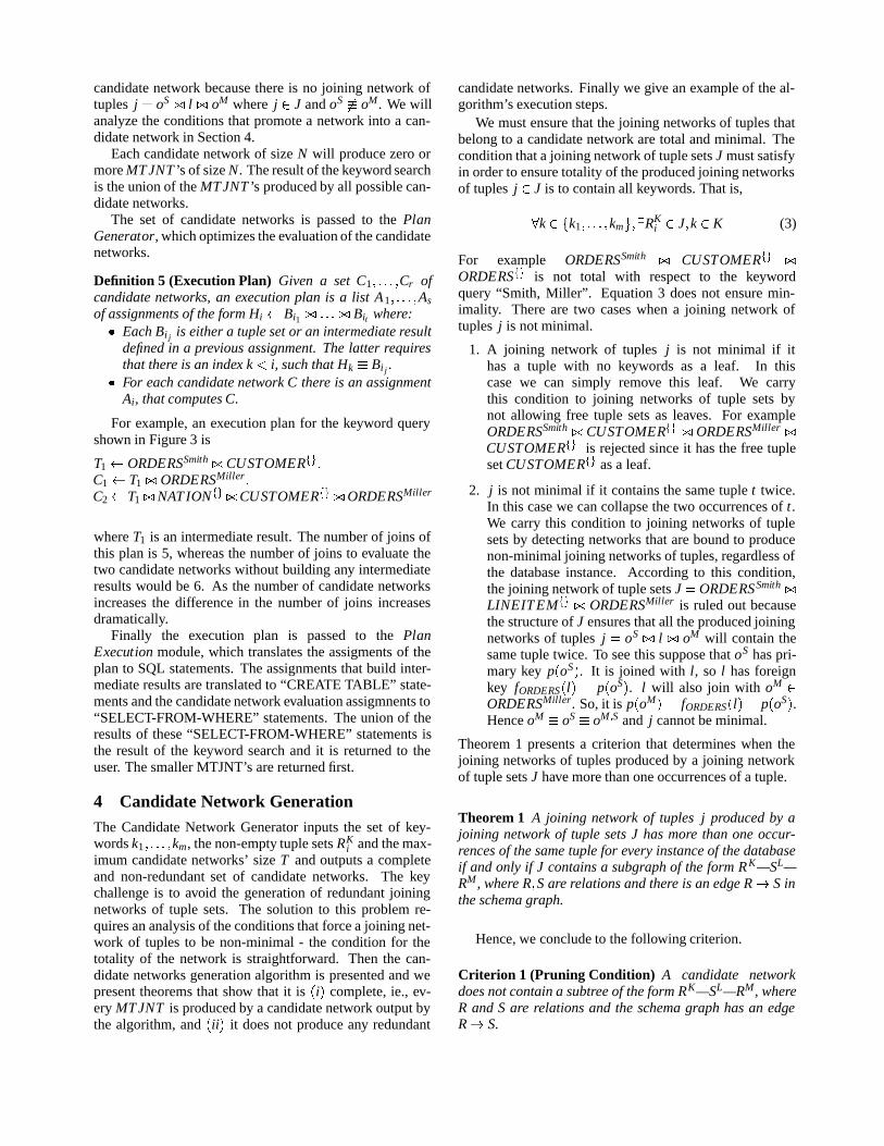
candidate network because there is no joining network oftuples j � oS �� l �� oM where j � J and oS �� oM. We willanalyze the conditions that promote a network into a can-didate network in Section 4.

Each candidate network of size N will produce zero ormore MT JNT ’s of size N. The result of the keyword searchis the union of the MT JNT ’s produced by all possible can-didate networks.

The set of candidate networks is passed to the PlanGenerator, which optimizes the evaluation of the candidatenetworks.

Definition 5 (Execution Plan) Given a set C1� � � � �Cr ofcandidate networks, an execution plan is a list A1� � � � �Asof assignments of the form Hi � Bi1 �� � � � �� Bit where:� Each Bi j is either a tuple set or an intermediate result

defined in a previous assignment. The latter requiresthat there is an index k � i, such that Hk � Bij .

� For each candidate network C there is an assignmentAi, that computes C.

For example, an execution plan for the keyword queryshown in Figure 3 is

T1 � ORDERSSmith ��CUSTOMER���

C1 � T1 �� ORDERSMiller�

C2 � T1 ��NAT ION�� ��CUSTOMER�� ��ORDERSMiller

where T1 is an intermediate result. The number of joins ofthis plan is 5, whereas the number of joins to evaluate thetwo candidate networks without building any intermediateresults would be 6. As the number of candidate networksincreases the difference in the number of joins increasesdramatically.

Finally the execution plan is passed to the PlanExecution module, which translates the assigments of theplan to SQL statements. The assignments that build inter-mediate results are translated to “CREATE TABLE” state-ments and the candidate network evaluation assigmnents to“SELECT-FROM-WHERE” statements. The union of theresults of these “SELECT-FROM-WHERE” statements isthe result of the keyword search and it is returned to theuser. The smaller MTJNT’s are returned first.

4 Candidate Network GenerationThe Candidate Network Generator inputs the set of key-words k1� � � � �km, the non-empty tuple sets RK

i and the max-imum candidate networks’ size T and outputs a completeand non-redundant set of candidate networks. The keychallenge is to avoid the generation of redundant joiningnetworks of tuple sets. The solution to this problem re-quires an analysis of the conditions that force a joining net-work of tuples to be non-minimal - the condition for thetotality of the network is straightforward. Then the can-didate networks generation algorithm is presented and wepresent theorems that show that it is �i� complete, ie., ev-ery MT JNT is produced by a candidate network output bythe algorithm, and �ii� it does not produce any redundant

candidate networks. Finally we give an example of the al-gorithm’s execution steps.

We must ensure that the joining networks of tuples thatbelong to a candidate network are total and minimal. Thecondition that a joining network of tuple sets J must satisfyin order to ensure totality of the produced joining networksof tuples j � J is to contain all keywords. That is,

k � �k1� � � � �km�� RKi � J�k � K (3)

For example ORDERSSmith �� CUSTOMER�� ��

ORDERS�� is not total with respect to the keywordquery “Smith, Miller”. Equation 3 does not ensure min-imality. There are two cases when a joining network oftuples j is not minimal.

1. A joining network of tuples j is not minimal if ithas a tuple with no keywords as a leaf. In thiscase we can simply remove this leaf. We carrythis condition to joining networks of tuple sets bynot allowing free tuple sets as leaves. For exampleORDERSSmith �� CUSTOMER�� �� ORDERSMiller ��

CUSTOMER�� is rejected since it has the free tupleset CUSTOMER�� as a leaf.

2. j is not minimal if it contains the same tuple t twice.In this case we can collapse the two occurrences of t.We carry this condition to joining networks of tuplesets by detecting networks that are bound to producenon-minimal joining networks of tuples, regardless ofthe database instance. According to this condition,the joining network of tuple sets J � ORDERSSmith ��

LINEIT EM�� �� ORDERSMiller is ruled out becausethe structure of J ensures that all the produced joiningnetworks of tuples j � oS �� l �� oM will contain thesame tuple twice. To see this suppose that oS has pri-mary key p�oS�. It is joined with l, so l has foreignkey fORDERS�l� � p�oS�. l will also join with oM �ORDERSMiller. So, it is p�oM� � fORDERS�l� � p�oS�.Hence oM � oS � oM�S and j cannot be minimal.

Theorem 1 presents a criterion that determines when thejoining networks of tuples produced by a joining networkof tuple sets J have more than one occurrences of a tuple.

Theorem 1 A joining network of tuples j produced by ajoining network of tuple sets J has more than one occur-rences of the same tuple for every instance of the databaseif and only if J contains a subgraph of the form RK—SL—RM, where R�S are relations and there is an edge R � S inthe schema graph.

Hence, we conclude to the following criterion.

Criterion 1 (Pruning Condition) A candidate networkdoes not contain a subtree of the form RK—SL—RM, whereR and S are relations and the schema graph has an edgeR� S.

�������� �� � ��� �������� ���������Input: tuple set graph GTS, T , k1� � � � �kmOutput: set of candidate networks with size up to T�

�� ����� �� ������� �������� �� ����� �������� � ������ kt � �k1� � � � �km���� ���� ����� ��� RK

i ����� i � 1� � � � �n �� kt � K �

� ������� �������� �� ����� ���� RKi �� Q

����� Q ��� ���� � ���� ��� C ��� Q�� C ��������� ��� ������� ��� ����� ���� ������ C���� �� C ��������� ��� ���������� ��� ������ ���� ������ C�� ���� �� �� ������ �� �!��� ������� ������� �������� �� ����� ����������

��� ���� ����� ��� RKi � ������ �� GTS "�������� � �� ��������# �� � �� � �� C

�� "K � �� $% � �RMj � �C�RK

i ��M �� ��� keywords�C�RKi � � keywords��C�RK

i ��RMj �#

��&!������� �������� "��'� �� C � T# ���� ��� RK

i �� � ������ �� RMj �� C � RM

j �� � �� ���� C RKi �RM

j �� � ���

��� C �� Q����� ������ RK

i� �

Figure 5: Algorithm for generating the candidate networks

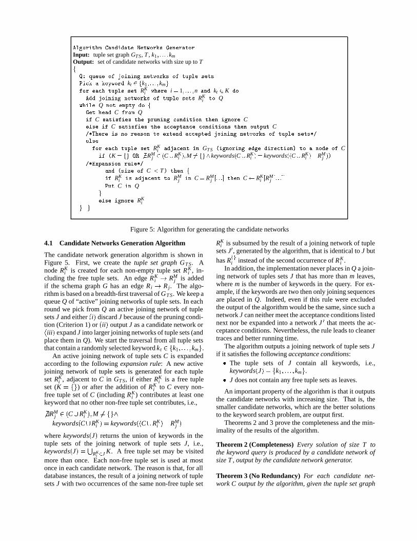
4.1 Candidate Networks Generation Algorithm

The candidate network generation algorithm is shown inFigure 5. First, we create the tuple set graph GT S. Anode RK

i is created for each non-empty tuple set RKi , in-

cluding the free tuple sets. An edge RKi � RM

j is addedif the schema graph G has an edge Ri � R j. The algo-rithm is based on a breadth-first traversal of GT S. We keep aqueue Q of “active” joining networks of tuple sets. In eachround we pick from Q an active joining network of tuplesets J and either �i� discard J because of the pruning condi-tion (Criterion 1) or �ii� output J as a candidate network or�iii� expand J into larger joining networks of tuple sets (andplace them in Q). We start the traversal from all tuple setsthat contain a randomly selected keyword kt � �k1� � � � �km�.

An active joining network of tuple sets C is expandedaccording to the following expansion rule: A new activejoining network of tuple sets is generated for each tupleset RK

i , adjacent to C in GT S, if either RKi is a free tuple

set (K � ��) or after the addition of RKi to C every non-

free tuple set of C (including RKi ) contributes at least one

keyword that no other non-free tuple set contributes, i.e.,

� RMj � �C�RK

i ��M �� ���

keywords�C�RKi � � keywords��C�RK

i �RMj �

where keywords�J� returns the union of keywords in thetuple sets of the joining network of tuple sets J, i.e.,keywords�J� �

�RK

i �J K. A free tuple set may be visitedmore than once. Each non-free tuple set is used at mostonce in each candidate network. The reason is that, for alldatabase instances, the result of a joining network of tuplesets J with two occurrences of the same non-free tuple set

RKi is subsumed by the result of a joining network of tuple

sets J�, generated by the algorithm, that is identical to J but

has R��i instead of the second occurrence of RK

i .In addition, the implementation never places in Q a join-

ing network of tuples sets J that has more than m leaves,where m is the number of keywords in the query. For ex-ample, if the keywords are two then only joining sequencesare placed in Q. Indeed, even if this rule were excludedthe output of the algorithm would be the same, since such anetwork J can neither meet the acceptance conditions listednext nor be expanded into a network J � that meets the ac-ceptance conditions. Nevertheless, the rule leads to cleanertraces and better running time.

The algorithm outputs a joining network of tuple sets Jif it satisfies the following acceptance conditions:� The tuple sets of J contain all keywords, i.e.,

keywords�J� � �k1� � � � �km�.� J does not contain any free tuple sets as leaves.

An important property of the algorithm is that it outputsthe candidate networks with increasing size. That is, thesmaller candidate networks, which are the better solutionsto the keyword search problem, are output first.

Theorems 2 and 3 prove the completeness and the min-imality of the results of the algorithm.

Theorem 2 (Completeness) Every solution of size T tothe keyword query is produced by a candidate network ofsize T , output by the candidate network generator.

Theorem 3 (No Redundancy) For each candidate net-work C output by the algorithm, given the tuple set graph

PART (P{}) ORDERS (O{})PARTSUPP (PS{}) LINEITEM (L{})

CUSTOMER (C{})ORDERSMiller (OMiller)

ORDERSSmith (OSmith)

NATION (N{})

SUPPLIER (S{})

REGION (R{})

Figure 6: Tuple set graph

# Queue/from/candidate networks output

1a OSmith

2a OSmith �� L��/1ab OSmith ��C��/1a3a OSmith

�� L�� �� O��(pruned)/2ab OSmith �� L�� �� OMiller(pruned)/2ac OSmith �� L�� �� PS��/2ad OSmith ��C�� �� O��/2be OSmith ��C�� �� OMiller/2bf OSmith ��C�� �� N��/2b4a OSmith

�� L�� �� PS�� �� P��/3c/ OSmith��C�� �� OMiller

b OSmith �� L�� �� PS�� �� L��/3cc OSmith ��C�� �� O�� ��C��(pruned)/3dd OSmith ��C�� �� N�� ��C��/3f

� � �

5a OSmith �� L�� �� PS�� �� P�� �� PS��(pruned)/4ab OSmith �� L�� �� PS�� �� L�� �� OMiller/4bc OSmith ��C�� �� N�� ��C�� �� OMiller /4dd OSmith ��C�� �� N�� ��C�� �� O��/4de OSmith ��C�� �� N�� ��C�� �� N��(pruned)/4d

� � �

6a OSmith �� C�� �� N�� �� C�� �� O�� �� C��(pruned)/5d/OSmith ��C�� �� N�� ��C�� �� OMiller

� � �/ /OSmith �� L�� �� PS�� �� L�� �� OMiller

7 � � �

Figure 7: Example

GT S2, there is an instance I of the database that produces

the same tuple set graph GT S, contains a MTJNT j �C andj does not belong to any other candidate network.

Example. We present the execution of the candidate net-work generator algorithm for the keyword query “Smith,Miller” on the TPC-H schema and the database instance inFigure 2, for T � 5. That is, we consider candidate net-works having at most 5 joins. The tuple set graph is shownin Figure 6.

Suppose we pick “Smith” as the kt of the algorithm.Hence we put ORDERSSmith into the queue. The state ofthe queue and the candidate networks output in each itera-tion are shown in Figure 7. We use the obvious abbreviatednames for the relations. Since the query has only two key-words, only joining sequences are generated and eventuallyoutput.Maximum size of candidate networks. Depending onthe form of the database schema, the maximum size Tmax

2Notice that the candidate network generator does not examine thetuples of a specific tuple set, but only whether it is empty or not.

of the candidate networks may be bounded or unboundedby the database schema.

Theorem 4 Tmax is unbounded if and only if G has one ofthe following properties:� There is a node of G that has at least two incoming

edges.� G has a directed cycle.

5 Evaluation of Candidate NetworksThe Plan Generator module of DISCOVER inputs a set ofcandidate networks and creates an execution plan to eval-uate them as defined in Section 3.2. The key optimiza-tion opportunity is that typically the candidate networksshare join subexpressions. Efficient execution plans storethe common join expressions as intermediate results andreuse them in evaluating the candidate networks. For ex-ample, in Figure 3 we calculate and store the join expres-sion ORDERSSmith �� CUSTOMER��. CUSTOMER�� ��

ORDERSMiller is also a common join expression but it willnot help to store both, as we explain below.

The space of execution plans that can be generated fora set of candidate networks is huge. We prune it by thefollowing two assumptions: First, we define every non-freetuple set to be a small relation, since its tuples are restrictedto contain specific keywords. The result of a join that in-volves a small relation is also a small relation. Those as-sumptions lead to the conclusion that every join expressionof the plan must contain a small relation and, hence, allintermediate results are small. Note that both the assump-tions and the conclusion follow directly the Wong-Yousefialgorithm ([Ull82]) of INGRES. Indeed, in practice, the in-termediate results are sufficiently small to be stored in mainmemory as we discuss in Section 6.

Second, the plan generator only considers planswhere the right hand side of the assignmentsHi � Bi1 �� � � � �� Bit of Definition 5 in Section 3.2are joins of exactly two arguments, i.e., t � 2. This policyis based on the assumption that the cost of calculatingand storing the results of both A �� B and A �� B �� C isessentially the same with the cost for just calculating andstoring the result of A �� B �� C, if the DBMS optimizerselects to first calculate A �� B and then the result ofA �� B �� C. Hence we can store and possibly reuse laterA �� B “for free”.

This assumption is very precise when there are indiceson the primary and foreign key attributes. Then the joins(and, in particular, the most expensive ones) are executedin a series of index-based 2-way joins. The assumptionalways held for the Oracle 8i DBMS that we used in ourTPC-H-based experimentation. (The assumption deviatesfrom reality when there are no indices and the databasechooses multi-way merge-sort joins.)

In summary, the plan generator considers and evaluatesthe space of plans where the joins have exactly two argu-ments. Note that once a plan P is selected from the re-stricted space we outlined, the plan generator eliminates

non-reused intermediate results by inlining their definitioninto the single point where they are used. That is, given twoassignments

T � A �� B

T � � T ��C

if T is not used at any other place than the computation ofT �, the two assignments will be merged into

T � � A �� B ��C

Cost Model. The theoretical study of the complexity ofselecting the optimal execution plan is based on a simplecost model of execution plans: We assign a cost of 1 toeach join. We use this theoretical cost model in proving thatthe selection of the optimal execution plan is NP-complete(Theorem 5). It is easy to see that the problem is also NP-hard for the actual cost model of DISCOVER.

The actual cost model of DISCOVER exploits the factthat we can get the sizes of the non-free tuple sets from themaster index. We also assume that we know the selectivityof the primary to foreign key joins, which can be calculatedfrom the sizes of the relations. The actual cost model de-fines the cost of a join to be the size of its result in numberof tuples. (The cost model can easily be modified to workfor the size in bytes instead of the number of tuples.) Thecost of the execution plan is the sum of the costs of its joins.Notice that since there are indices on the primary and for-eign keys, the cost of a join is proportional to the size of itsresult, since the joins will typically be index-based joins.

The problem of deciding which intermediate results tobuild and store can be formalized as follows:

Problem 1 (Choice of intermediate results) Given a setof candidate networks, find the intermediate results thatshould be built, so that the overall cost of building theseresults and evaluating the candidate networks is minimum.

Theorem 5 shows that Problem 1 is NP-complete on thesize of the candidate networks with respect to the theoreti-cal cost model defined above.

Theorem 5 Problem 1 is NP-complete.

5.1 Greedy algorithm

Figure 8 shows a greedy algorithm that produces a near-optimal execution plan, with respect to the actual costmodel defined above, for a set of candidate networks bychoosing in each step the join m between two tuple sets orintermediate results that maximizes the quantity f requencya

logb�size�,

where f requency is the number of occurences of m in thecandidate networks, size is the estimated number of tuplesof m and a�b are constants. The f requencya term of thequantity maximizes the reusability of the intermediate re-sults, while the logb�size� term minimizes the size of theintermediate results that are computed first. We have exper-imented with multiple combinations of values for a and band found that the optimal solution is closer approximated

�������� (����� ���� �� ������ ���� �������Input: set S of candidate networks of size TOutput: list L of intermediate results to build������ ��� ��� ��� � ��� �������� �� S ��)�

*��� � � �� L � �+�� Z *� ��� ��� �� ��� ���� ����

��*�!��������� �� 1 ���� �������� ���� ����� ��� ��� � ��� ������� �� S,

� ��� ������ ���� ������ m ���� ���

�!��� f requencya

logb�size� )���� �� Z �� L,

%������ ��� ��� � ��� �������� �� S �� ���m ����� �����*��,

��

Figure 8: Greedy algorithm for selecting a list of interme-diate results to build

for �a�b�� �1�0�, when the size of the candidate networks(and the reusability) increases.

We perform a worst case time analysis of the greedy al-gorithm. The while loop is executed at most �S� �T times ifevery join has a frequency of 1, where �S� is the number ofcandidate networks. The calculation of Z takes time �S� �T .We assume that we traverse a candidate network of size T1in time O�T1�. In each step, we keep a hash table H witheach intermediate result in Z and its frequency. Hence wecheck if an intermediate result is already in H and increaseits frequency in O�1�. Finding the intermediate result in Hthat maximizes f requencya

logb�size�takes time �S� �T . The rewriting

step also takes time �S� �T . Hence the total execution timetakes in the worst case time O���S� �T �2�.

The greedy algorithm may output a non optimal list ofintermediate results. However, in special cases the greedyis guaranteed to produce the optimal plan. One such caseis described by the theorem below:

Theorem 6 The greedy algorithm for �a�b� � �1�0� is op-timal for m � 2 keywords, when each of them is containedin exactly one relation.

6 ExperimentsWe evaluate the algorithms of DISCOVER with detailedperformance evaluation on a TPC-H database. First wemeasure the pruning efficiency of the candidate networkgenerator. In particular, we measured how many joiningnetworks of tuple sets are ruled out based on the pruningconditions of the candidate network generator. Then wecompare the plans produced by the greedy to the ones pro-duced by the optimal, where the optimal execution plan iscomputed using an exhaustive algorithm. We also com-pare the speedup in runtime performance for generatingand executing the execution plan using the greedy and theoptimal algorithm compared to the naive method, whereno intermediate results are built. Finally, we compare theoverall execution times of DISCOVER for some typical

#keyw JNTS K JNTS L CNs neTS’s2 25 5.355 4.485 2.963 55.22 13.86 9.27 4.354 85.69 33.88 24.03 5.915 101 37.3 26 7.12

(a) Fix maximum candidate networks’ size to 3MaxCNsize JNTS K JNTS L CNs neTS’s1 0.95 0.95 0.95 2.962 3.72 2.36 2.12 2.963 29.22 4.74 3.7 2.964 422.88 10.36 6.4 2.965 6941 24.75 11.45 2.96

(b) Fix number of keywords to 2MaxCNsize JNTS K JNTS L CNs neTS’s1 0.59 0.59 0.59 4.352 5.01 3.91 3.35 4.353 55.22 13.86 9.27 4.354 639.61 50.49 29.51 4.355 7532 223 103.66 4.35

(c) Fix number of keywords to 3

Figure 9: Evaluation of the candidate network generator

keyword queries to the naive method and to the optimalmethod.

We use the TPC-H database to conduct the experiments.The size of the database is 100MB. We use Oracle 9i,running on a Xeon 2.2GHz PC with 1GB of RAM. DIS-COVER has been implemented in Java and connects to theDBMS through JDBC. The master index is implementedusing the full-text Oracle9i interMedia Text extension. Thebasic tuple set of relation R for keyword k is produced bymerging the tuples returned by the full-text index on eachattribute of R. We found out that each keyword is containedon the average in 3�5 relations, that is, 3�5 non-empty basictuple sets are created for each keyword.

The tuple sets and the intermediate results are stored intables in the KEEP buffer pool of Oracle 9i, which retainsobjects in memory, thus avoiding I/O operations. We dedi-cated 70MB to the KEEP buffer pool. The display time isnot included in the measured execution time.

The naive method does not produce any intermediate re-sults – it simply executes each candidate network. The ex-ecution times for both the naive method and DISCOVER’sevaluation method, which builds and reuses intermediateresults, depend on the status of the cache of the DBMS.In order to eliminate this factor we warm-up the cachebefore executing the experiments. The warm-up is doneby executing the SQL queries corresponding to the candi-date networks produced by the candidate network genera-tor. Hence, we are certain that the warm-up does not favorDISCOVER more than the naive method.Evaluation of the candidate network generator. This ex-periment measures the pruning capabilities of the candi-date network generator. We use the TPC-H schema but wedo not use the TPC-H dataset in this experiment, becausewe want to control the distribution of the number of occur-rences of each keyword. So, we randomly put the keywordsof the keyword query in the relations. Each keyword is

#keyw Cost�O�Cost�G�

2 13 0.964 0.965 0.97

MaxCN Cost�O�Cost�G�

1 12 13 0.964 0.935 0.90

(a) Fix CN size to 3 (b) Fix # keywords to 3

Figure 10: Evaluation of the Plans of the Greedy Algorithm

contained in a relation R with probability a � log�size�R��,where size�R� is the number of tuples in R as defined inthe TPC-H specifications for scale factor SF=1. We se-lected a � 1

10�log2�6�000�000� . This means that the probabil-ity that a keyword is contained in the LINEIT EM relation,which is the largest one, is 1

10 , since size�LINEIT EM� �

6�000�000. This probability is about 1100 for the REGION

relation, which is the smallest one. We measure three num-bers of joining networks of tuple sets for each execution ofthe experiment.

1. JNT S K is the number of joining networks of tuplesets of size up to T that have the following properties:� They contain all keywords of the keyword query,

i.e., they are total.

� No non-free tuple set can be replaced by a freetuple set and still have all keywords in the join-ing network of tuple sets.

2. JNT S L is the number of joining networks of tuplesets that have only non-free tuple sets as leaves in ad-dition to the above properties.

3. CNs is the number of candidate networks generatedby DISCOVER. Those candidate networks have onemore property in addition to the above properties; theydo not produce joining networks of tuples with morethan one occurrences of the same tuple (Criterion 1).

We also measure the number of non-empty basic tuple sets(neTS’s) generated in each execution. Figure 9 shows theaverage results of the experiment for 1000 executions. No-tice that the ratio CNs

JNT S L decreases as the maximum sizeof the output candidate networks increases, i.e., Criterion 1prunes more when the candidate networks are larger. Thereason is that the trigger of Criterion 1 has more places tohappen in a large candidate network.Quality of Greedy. The quality of the plans produced bythe greedy algorithm are very close to the quality of theplans produced by the optimal. We use the same settingswith the above experiment. In Figure 10 we show how wellthe plans produced by the greedy algorithm perform on theaverage, compared to the optimal plans for �a � 1�b � 0�for 50 executions. In about 70% of the cases the generatedplans turn out to be identical and in the cases where theyare different, the differences are fairly small.Evaluation of Plan Generator. In this experimentwe measure the speedup that DISCOVER’s plan genera-tor induces. In particular, we compare the time spent inDISCOVER’s Plan Generator and Plan Execution modulesagainst the baseline provided by the naive method. We

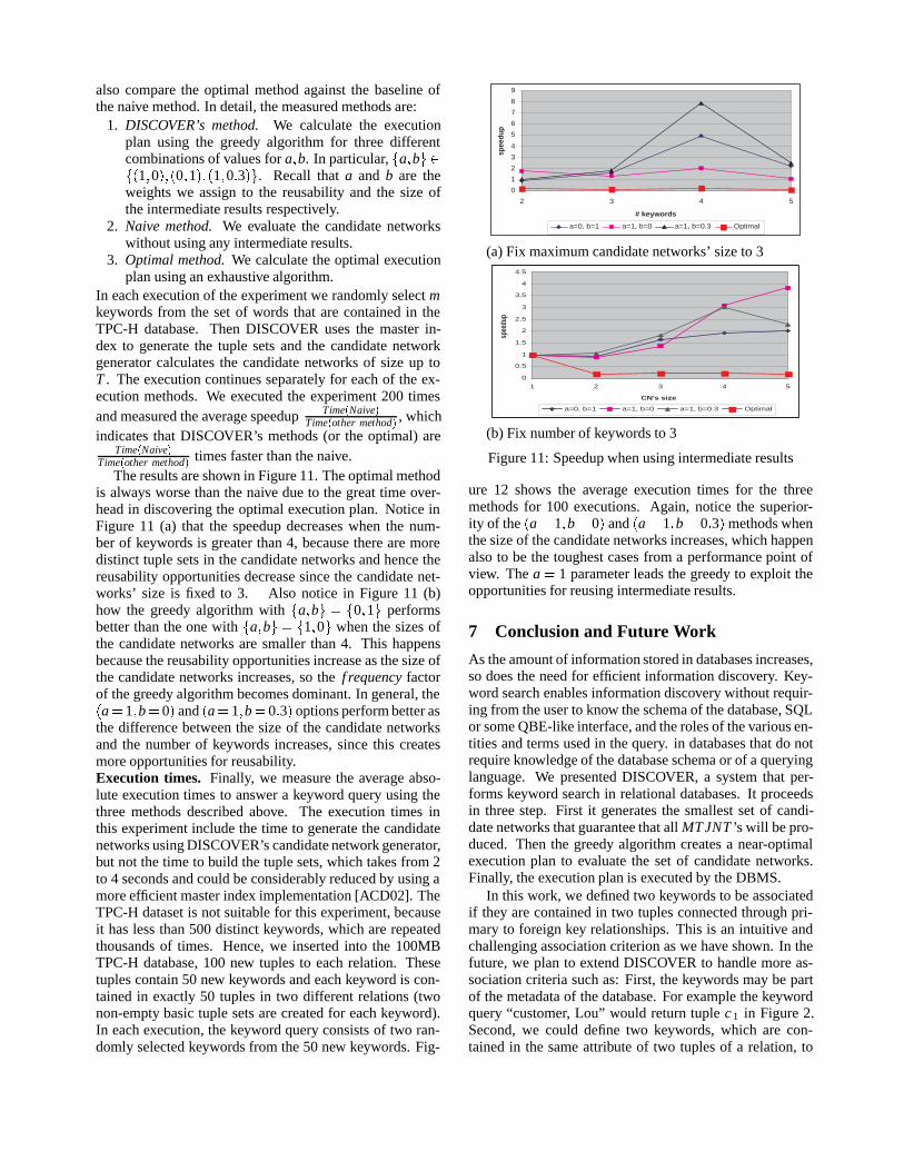
also compare the optimal method against the baseline ofthe naive method. In detail, the measured methods are:

1. DISCOVER’s method. We calculate the executionplan using the greedy algorithm for three differentcombinations of values for a�b. In particular, �a�b� ���1�0���0�1���1�0�3��. Recall that a and b are theweights we assign to the reusability and the size ofthe intermediate results respectively.

2. Naive method. We evaluate the candidate networkswithout using any intermediate results.

3. Optimal method. We calculate the optimal executionplan using an exhaustive algorithm.

In each execution of the experiment we randomly select mkeywords from the set of words that are contained in theTPC-H database. Then DISCOVER uses the master in-dex to generate the tuple sets and the candidate networkgenerator calculates the candidate networks of size up toT . The execution continues separately for each of the ex-ecution methods. We executed the experiment 200 timesand measured the average speedup Time�Naive�

Time�other method� , whichindicates that DISCOVER’s methods (or the optimal) are

Time�Naive�Time�other method� times faster than the naive.

The results are shown in Figure 11. The optimal methodis always worse than the naive due to the great time over-head in discovering the optimal execution plan. Notice inFigure 11 (a) that the speedup decreases when the num-ber of keywords is greater than 4, because there are moredistinct tuple sets in the candidate networks and hence thereusability opportunities decrease since the candidate net-works’ size is fixed to 3. Also notice in Figure 11 (b)how the greedy algorithm with �a�b� � �0�1� performsbetter than the one with �a�b�� �1�0� when the sizes ofthe candidate networks are smaller than 4. This happensbecause the reusability opportunities increase as the size ofthe candidate networks increases, so the f requency factorof the greedy algorithm becomes dominant. In general, the�a � 1�b� 0� and �a � 1�b � 0�3� options perform better asthe difference between the size of the candidate networksand the number of keywords increases, since this createsmore opportunities for reusability.Execution times. Finally, we measure the average abso-lute execution times to answer a keyword query using thethree methods described above. The execution times inthis experiment include the time to generate the candidatenetworks using DISCOVER’s candidate network generator,but not the time to build the tuple sets, which takes from 2to 4 seconds and could be considerably reduced by using amore efficient master index implementation [ACD02]. TheTPC-H dataset is not suitable for this experiment, becauseit has less than 500 distinct keywords, which are repeatedthousands of times. Hence, we inserted into the 100MBTPC-H database, 100 new tuples to each relation. Thesetuples contain 50 new keywords and each keyword is con-tained in exactly 50 tuples in two different relations (twonon-empty basic tuple sets are created for each keyword).In each execution, the keyword query consists of two ran-domly selected keywords from the 50 new keywords. Fig-

0

1

2

3

4

5

6

7

8

9

2 3 4 5

# keywords

spee

dup

a=0, b=1 a=1, b=0 a=1, b=0.3 Optimal

(a) Fix maximum candidate networks’ size to 3

0

0.5

1

1.5

2

2.5

3

3.5

4

4.5

1 2 3 4 5

CN's size

spee

dup

a=0, b=1 a=1, b=0 a=1, b=0.3 Optimal

(b) Fix number of keywords to 3

Figure 11: Speedup when using intermediate results

ure 12 shows the average execution times for the threemethods for 100 executions. Again, notice the superior-ity of the �a � 1�b � 0� and �a � 1�b � 0�3� methods whenthe size of the candidate networks increases, which happenalso to be the toughest cases from a performance point ofview. The a � 1 parameter leads the greedy to exploit theopportunities for reusing intermediate results.

7 Conclusion and Future Work

As the amount of information stored in databases increases,so does the need for efficient information discovery. Key-word search enables information discovery without requir-ing from the user to know the schema of the database, SQLor some QBE-like interface, and the roles of the various en-tities and terms used in the query. in databases that do notrequire knowledge of the database schema or of a queryinglanguage. We presented DISCOVER, a system that per-forms keyword search in relational databases. It proceedsin three step. First it generates the smallest set of candi-date networks that guarantee that all MT JNT ’s will be pro-duced. Then the greedy algorithm creates a near-optimalexecution plan to evaluate the set of candidate networks.Finally, the execution plan is executed by the DBMS.

In this work, we defined two keywords to be associatedif they are contained in two tuples connected through pri-mary to foreign key relationships. This is an intuitive andchallenging association criterion as we have shown. In thefuture, we plan to extend DISCOVER to handle more as-sociation criteria such as: First, the keywords may be partof the metadata of the database. For example the keywordquery “customer, Lou” would return tuple c 1 in Figure 2.Second, we could define two keywords, which are con-tained in the same attribute of two tuples of a relation, to

1

10

100

1000

10000

100000

1000000

10000000

1 2 3 4 5

CN's size

mse

cs

a=0, b=1 a=1, b=0 a=1, b=0.3 Naive Optimal

(a) Fix number of keywords to 2

1

10

100

1000

10000

100000

1000000

10000000

1 2 3 4 5

CN's size

mse

cs

a=0, b=1 a=1, b=0 a=1, b=0.3 Naive Optimal

(b) Fix number of keywords to 3

Figure 12: Execution times

be associated. For example, the tuples o1�o2 are a solutionto the keyword query “Smith, Miller”, by this criterion.

We plan to apply new optimization techniques to DIS-COVER. For example we plan to apply dynamic optimiza-tion techniques in the evaluation of the candidate networks.Currently, DISCOVER uses static optimization methods.That is, the whole execution plan is generated before itsevaluation begins. Furthermore, we plan to experimentwith new cost models that access the DBMS’s optimizer.We are also building from scratch a more efficient masterindex.

Finally, we are working on building polynomial time al-gorithms that generate an optimal execution plan for specialcases of database schemas.

8 Acknowledgements

We wish to thank Charles Elkan for providing the problem.We also thank Nick Koudas for the discussions we madeand the ideas he proposed.

References[ACD02] Sanjay Agrawal, Surajit Chaudhuri, and Gautam

Das. DBXplorer: A System For Keyword-BasedSearch Over Relational Databases. ICDE, 2002.

[ACGM�01] Arvind Arasu, Junghoo Cho, Hector Garcia-Molina, Andreas Paepcke, and Sriram Raghavan.Searching the web. Transactions on Internet Tech-nology, 2001.

[AHV95] S. Abiteboul, R. Hull, and V. Vianu. Foundationsof Databases. Addison Wesley, 1995.

[BNH�02] G. Bhalotia, C. Nakhey, A. Hulgeri, S. Chakrabarti,and S. Sudarshanz. Keyword Searching and

Browsing in Databases using BANKS. Proceed-ings of International Conference on Data Engi-neering, 2002.

[BP98] S. Brin and L. Page. The Anatomy of a Large-ScaleHypertextual Web Search Engine. WWW Confer-ence, 1998.

[DB201] http://www.ibm.com/software/data/db2/extenders/textinformation/index.html. 2001.

[Fin82] Sheldon J. Finkelstein. Common subexpressionanalysis in database applications. ACM SIGMOD,1982.

[FKM99] Daniela Florescu, Donald Kossmann, and IoanaManolescu. Integrating Keyword Search into XMLQuery Processing. WWW9 Conference, 1999.

[GSVGM98] R. Goldman, N. Shivakumar, S. Venkatasubrama-nian, and H. Garcia-Molina. Proximity Search inDatabases. VLDB, 1998.

[MSD01] http://msdn.microsoft.com/library/. 2001.

[MV00a] U. Masermann and G. Vossen. Schema Indepen-dent Database Querying (on and off the Web).Proc. Of IDEAS2000, 2000.

[MV00b] Ute Masermann and Gottfried Vossen. Designand Implementation of a Novel Approach to Key-word Searching in Relational Databases. ADBIS-DASFAA Symposium, 2000.

[Ora01] http://technet.oracle.com/products/text/content.html. 2001.

[Ple81] J. Plesn’ik. A bound for the Steiner tree problem ingraphs. Math. Slovaca 31, pages 155–163, 1981.

[RSSB00] Prasan Roy, S. Seshadri, S. Sudarshan, and Sid-dhesh Bhobe. Efficient and extensible algorithmsfor multi query optimization. SIGMOD Record,29(2):249–260, 2000.

[Sal89] Gerard Salton. Automatic Text Processing: TheTransformation, Analysis, and Retrieval of Infor-mation by Computer. Addison Wesley, 1989.

[Sel88] Timos K. Sellis. Multiple-query optimization.TODS, 13(1):23–52, 1988.

[SS82] J. A. Storer and T. Szymanski. Data Compressionvia Textual Substitution. J.ACM, 1982.

[TWW�00] Jason T., L. Wang, Xiong Wang, Dennis Shasha,Bruce A. Shapiro, Kaizhong Zhang, Qicheng Ma,and Zasha Weinberg. An approximate search en-gine for structural databases. SIGMOD, 2000.

[Ull82] Jeffrey D. Ullman. Principles of Database Systems,2nd Edition. Computer Science Press, 1982.