discovering local patterns of co - evolution: computational

RESEARCH ARTICLE Open Access

Discovering local patterns of co - evolution:computational aspects and biological examplesTamir Tuller1,2,3,4*, Yifat Felder1, Martin Kupiec2

Abstract

Background: Co-evolution is the process in which two (or more) sets of orthologs exhibit a similar or correlativepattern of evolution. Co-evolution is a powerful way to learn about the functional interdependencies between setsof genes and cellular functions and to predict physical interactions. More generally, it can be used for answeringfundamental questions about the evolution of biological systems.Orthologs that exhibit a strong signal of co-evolution in a certain part of the evolutionary tree may show a mildsignal of co-evolution in other branches of the tree. The major reasons for this phenomenon are noise in the bio-logical input, genes that gain or lose functions, and the fact that some measures of co-evolution relate to rareevents such as positive selection. Previous publications in the field dealt with the problem of finding sets of genesthat co-evolved along an entire underlying phylogenetic tree, without considering the fact that often co-evolutionis local.

Results: In this work, we describe a new set of biological problems that are related to finding patterns of local co-evolution. We discuss their computational complexity and design algorithms for solving them. These algorithmsoutperform other bi-clustering methods as they are designed specifically for solving the set of problemsmentioned above.We use our approach to trace the co-evolution of fungal, eukaryotic, and mammalian genes at high resolutionacross the different parts of the corresponding phylogenetic trees. Specifically, we discover regions in the fungitree that are enriched with positive evolution. We show that metabolic genes exhibit a remarkable level of co-evo-lution and different patterns of co-evolution in various biological datasets.In addition, we find that protein complexes that are related to gene expression exhibit non-homogenous levels ofco-evolution across different parts of the fungi evolutionary line. In the case of mammalian evolution, signalingpathways that are related to neurotransmission exhibit a relatively higher level of co-evolution along the primatesubtree.

Conclusions: We show that finding local patterns of co-evolution is a computationally challenging task and weoffer novel algorithms that allow us to solve this problem, thus opening a new approach for analyzing theevolution of biological systems.

1 BackgroundCo-evolution is the process by which two (or more) setsof orthologs exhibit a similar or a correlative pattern ofevolution. Co-evolution can be measured in variousways; those most commonly used are: the similarity inabsolute Evolutionary Rate (ER; dN; the rate of non-synonymous substitutions) or dN/dS (the rate of non-synonymous substitutions rate divided by the rate ofsynonymous substitutions) [1-3], correlative ER or dN/

dS [4-6], and similarity in the pattern of protein pre-sence in the proteomes of a set of organisms [7-9].Detecting co-evolving sets of orthologs is an importantmatter since physically interacting proteins [4,5,10,11]and functionally related proteins [1,3,6,12,13] tend toco-evolve. Thus, an appropriate analysis of co-evolvinggenes can lead to a better understanding of the evolu-tion of various cellular processes and gene modules (e.g.see [14] and [15]).The most popular approach for detecting co-evolution

is based on phylogenetic profiles [7-9]. It searches* Correspondence: [email protected] of Computer Science, Tel Aviv University, Tel Aviv, Israel

Tuller et al. BMC Bioinformatics 2010, 11:43http://www.biomedcentral.com/1471-2105/11/43

© 2010 Tuller et al; licensee BioMed Central Ltd. This is an Open Access article distributed under the terms of the Creative CommonsAttribution License (http://creativecommons.org/licenses/by/2.0), which permits unrestricted use, distribution, and reproduction inany medium, provided the original work is properly cited.

mailto:[email protected]

http://creativecommons.org/licenses/by/2.0

groups of orthologs with similar phyletic patterns. Themain disadvantage of this approach is the fact that ittotally ignores the topology of the organisms’ evolution-ary tree. A similar measure is the Propensity for GeneLoss (PGL) in evolution [12,13,16]. Genes with lowerPGL have lower ER and tend to be essential for the via-bility of the organism. It has been proven recently [13]that orthologs with correlative PGL tend to be function-ally related.Another related measure for evolutionary distance is

the difference between the average dN/dS or ER of pairsof orthologs [1-3]. Using this measure Marino et al.showed that there is a strong connection between thefunction of genes and their evolutionary rates [3]. Allprevious approaches for detecting co-evolution have notconsidered the fact that gene modules can exhibit strongpatterns of co-evolution in some parts of the evolution-ary tree while exhibiting a very weak signal of co-evolu-tion in other periods of their evolution. There may be anumber of reasons for this phenomenon.First, evolving genes may gain or lose functions (see e.

g. [17]); loss or gain of a new function can move anortholog from one co-evolving module to a differentone. Additionally, there may be differences in evolution-ary pressure acting within ortholog groups in differentparts of the evolutionary tree (see e.g. [18]). Second, theanalyzed biological data may be noisy or partial in someportions of an evolutionary tree while it can have higherquality in other parts. In such cases, searching sets oforthologs with similar evolution along the entire phylo-genetic tree may result in high false negative rates.Third, there are co-evolutionary problems that are localby definition. For example, genes tend to undergo posi-tive selection in a small fraction of their history (see e.g.[19]). Thus, if we define co-evolution as a process inwhich a set of orthologs undergoes positive selectiontogether, we should not expect that such type of co-evo-lution should span the entire phylogenetic tree.The goal of this work is to study the Local Co-Evolu-

tionary problem. Namely, given a phylogenetic treeand a set of vectors describing the evolution of ortho-logous sets along the evolutionary tree we aim to find

sub-sets of orthologs with similar evolution along sub-trees of the evolutionary tree (see Figure 1C). We for-malize a new set of Local Co-Evolutionary problems,study their computational hardness and describe algo-rithms and heuristics for solving them. A simulationstudy shows that these algorithms give much betterperformances than popular bi-clustering algorithms forgene expression. Finally, we generate five relevant bio-logical datasets and use our computational tools toanalyze them. Three datasets include dN/dS and geneCopy Number (CN) of thousands of orthologs acrossevolutionary trees. The two other datasets include thedN/dS and CN related to hundreds of signaling path-ways and protein complexes across evolutionary treeswith dozens of nodes.

2 Definitions and PreliminariesAs was mentioned in the Introduction, in this work theaim is to find sets of orthologs with similar evolutionaryalong parts (subtrees) of the evolutionary tree. In thissection, we formally define this problem. Furthermore,we define several measures of co-evolution and a fewpossible inputs to our problem.Let T = (V, E) be a tree, where V and E are the tree

nodes and tree edges respectively. In this work, we con-sider rooted binary phylogenetic trees (i.e. the degree ofeach node in the tree is either 1, 2, or 3), and all thetrees that are described in this work are species trees. Anode of degree 1 is named a leaf, a node with degree 3is named an internal node, and the root has degree 2. Atree T’ is a subtree of T if it is a connected subgraph inT. We denote such a relation by T’ ⊆ T. Note that bythe above definition an internal node of a tree T can bea leaf in the subtree T’ ⊆ T.A Node Orthologous Labeling (NOL) of a tree T, is a

set of labels (real numbers) for each of the nodes in T;an Edge Orthologous Labeling (EOL) for a tree T, is a setof labels for each of the edges in T (see Figure 1). AnOrthologous Labeling (OL, i.e. a NOL or EOL) of a treereflects the evolutionary patterns along the tree. Thus,we also name the OL of a tree: the evolutionary patternalong the tree.

Edge Orthologs Labeling 1



(h,k) (i,k) (c,i) (d,i) )i,k()h,b(Evolutionary Rate

Edge




a b c d e f g

h i j

k

l

1 2 1 1 0 0 1

2 2 1

2

1

A. .C.B

0.1

1.5

0.3

1

0.2 0.4

0.6

0.20.1

0.70.1

Figure 1 A. A hypothetic example of a node orthologous labeling which includes gene copy number in each node of the evolutionarytree. B. A hypothetic example of an edge orthologous labeling which includes dN/dS along each edge of the evolutionary tree. C. The goal ofthe local co-evolutionary problem is to find large sets of orthologs that have similar patterns of evolution across large subtrees of theevolutionary tree.


of 19

Let S denote a set of OLs in T, and let S’ be a subsetof S. Let Dc(S’, T’) denote a measure for co-evolutionalong a subtree, T’ ⊆ T. Such a measure returns a realpositive number which reflects how similar is the co-evolution of the OLs from S’ along the subtree T’ (0reflects an identical evolution). Formally, we deal withversions of the following problem:Problem 1 Local Co-EvolutionInput: A phylogenetic tree, T = (V, E), a set of NOLs or

EOLs, S = [S1,.., Sm], two natural numbers, n’, m’, a realnumber, d, and a measure of co-evolution, Dc(.,.). Ques-tion: Is there a subtree T’ = (V’, E’) ⊆ T with |E’| = n’, anda subset S’ ⊆ S with |S’| = m’, such that Dc(S’, T’) ≤ d ?In the rest of this section we describe a few examples

of NOLs and EOLs, and give a few examples of mea-sures of co-evolution.In this work, we analyzed one NOL:(1) Gene copy number of orthologs, which is the

number of paralogs of a given gene (from a certainorthologous group) in each node (genome and ancestralgenome) of the evolutionary tree. In general, we candeal both with absolute values and discrete values ofgene copy numbers. In the discrete case, we are onlyinterested in whether a certain ortholog appears or notin each node of the evolutionary tree and not in thenumber of times it appears, while in the absolute valuewe do consider the number of times each orthologappears in each node of the evolutionary tree.We also analyzed two EOLs:(1) Non-synonymous substitution rate, dN, divided

by the synonymous substitution rate, dS (i.e. dN/dS).We examined absolute, discrete, and relative values ofdN/dS. The absolute case is dN/dS (a positive realnumber) without additional processing. In the discretecase, we only consider three possibilities: dN/dS > 1(positive selection, dN/dS > 1), dN/dS ≈ 1 (neutralselection, dN/dS ≈ 1), or dN/dS < 1 (purifying selec-tion, dN/dS <1). In the relative case, we perform anadditional normalization of the dN/dS of each ortholo-gous group by comparing them to the dN/dS of otherorthologous groups. This is done by computing for

each edge of the tree the rank of the dN/dS of anorthologous group among the dN/dS of all orthologousgroup.(2) Change in orthologous gene Copy Numbers

(CN) along the tree edges. In this case, we can checkthe exact changes or only the direction of the changes(i.e. if the copy number increases, decreases, or does notchange along an edge).We analyzed the following measures of co-evolution

(Figure 2; we usually give examples that are related todN/dS but with the appropriate changes all the mea-sures can be implemented on NOLs and on labelingsthat are related to CNs):(1) D S S S S Tc1 1 2 f( [ , ,.., ], ) is the maximal L1 norm

between all the pairs of S S S f1 2, ,.., along the evolu-

tionary subtree T’. Dc1 measures the similarity of theabsolute values in the OLs (see Figure 2A). Thus, ortho-logs that have similar dN/dSs along each branch of T’will have a significantly low Dc1.(2) D S S S S Tc2 1 2 f( [ , ,.., ], ) | | 1 r , where r

denotes the minimal Spearman correlation among all

pairs of the OL of S S S f1 2, ,.., along the edges or nodes

of T’. Orthologs can differ in their average dN/dS butexhibit similar fluctuations in their ER (see Figure 2B).Dc1 can not discover such pattern of co-evolution butDc2, as it finds sets of orthologs with correlative patternof evolution, is suitable for this task.

(3)D S S S S T E Vc3 1 2 f( [ , ,.., ], ( , )) | |

|{ : ( ),

E

e E S e1 (( ) .. ( )}|, , S Se f e2 where ℓ is a certain labeling. This measure is used forfinding a large subtree and a set of orthologs with iden-tical labeling along most of this subtree (see Figure 2C).In this work, we used this measure for finding a sub-

tree where a set of orthologs undergoes positive selec-tion (i.e. dN/dS >1) together. To this end, we firstperformed a two-level discretization of the dN/dSvalues; one discrete level was assigned to the dN/dSabove 1 and the second discrete level was assigned tothe dN/dS below 1.

DC4

(h,k) (k,l) (l,m) (m,n)

OL1

EREdge

OL2

OL3

OL4

E.

~

~

~

~

(n,i)(n,i) (n,j) (j,d) (j,c)

OL1

EREdge

OL2

OL3

OL4

A. DC1

OL'1

EREdge

OL'2

OL'3

OL'4

(h,k) (g,k) (k,l) (l,f)

B. DC2

abcdefgh

ijkl

C.m

n(l,m) (m,e) (m,n) D.

DC3

OL''1ER

Edge

OL''2

OL''3

OL''4

1 1 1 001 1 1 01

1 1 1 101 1 1 00

Figure 2 Illustration of the four measures of local co-evolution (A. Dc1, B. Dc2, D. Dc3 and E. Dc4) along a hypothetical evolutionary tree(C.). A. In the case of Dc1, the co-evolution score is high when values of all the OLs along a sub-tree are similar. B. In the case of Dc2, the co-evolution score is high when values of all the OLs along a sub-tree are correlative (i.e. the OLs tend increase/decrease on the same branches). D.Dc3 is used for finding a large subtree and a set of orthologs with identical labeling along most of a subtree. E. Dc4 is used for finding sets oforthologs that have similar monotonic/non-monotonic decreasing/increasing evolutionary pattern along a path.


of 19

(4) Dc4(S’, T’): In the case of Dc4(S’, T’), we want tofind a path along the evolutionary tree (i.e. T’ is a path),and a set of OLs, S’, that have similar monotonic/non-monotonic decreasing/increasing evolutionary patternalong the path (see Figure 2D).Dc4(S’, T’) = d denotes that the maximal number of

components of an orthologous labeling, Si Î S’, thatshould be changed in order to fit them to the patternthat the path induces is less than d. This measure can beuseful for discovering modules of orthologs that exhibittogether acceleration or deceleration in their ER or dN/dS along a certain evolutionary path due to speciation.

3 Hardness IssuesHardness issues that are related to the Local Co-Evolu-tionary problem appear in additional files 1 and 2.Specifically, in this note, we show that some versionsof the problem are NP-hard, but in practice it seemsthat the Local Co-Evolutionary problem has a shorterrunning time than the bi-clustering problem which ishighly used in the context of gene expression analysis.Furthermore, we show that there are versions of theLocal Co-Evolutionary problem that can be solved by a

fixed-parameter tractable (FPT) algorithm or by a poly-nomial algorithm.

4 Methods4.1 Heuristics and AlgorithmsThis section includes a description of the two algo-rithms that we developed for finding local patterns ofco-evolution. The goal of these algorithms is to find co-evolving sets with at least m’ OL, that exhibit co-evolu-tion score <d along a tree with more than n’ edges. Thethreshold d determines the sizes of the subtrees in thesolutions. It is easy to see that on average OLs corre-sponding to larger subtrees have higher co-evolutionaryscore. Thus, larger d will result in solutions with largersubtrees while smaller d will result in solutions withsmaller subtrees.We designed two main algorithms. The first algo-

rithm, the Tree Grower, starts with sets of orthologswith similar patterns of evolution along small subtrees,and expands these initial trees while possibly decreasingthe set of orthologs (Figure 3B). The second algorithm,the Tree Splitter, finds first sets of orthologs with similarpattern of evolution along the entire input tree, and

A. Input:

Tree Splitter

hg i

j

A phylogenetic tree

OL1

OL2

OL3

OL5

OLn

OL4

OL6

OL7 . .

A set oforthologous

labelings

a b c d e fTree Grower

OL71 OL21OL452

OL80

OL79

OL40

OL321

OL71OL452

OL80

OL79

OL40

OL321

OL6

OL5

OL62

OL3

OL6

OL5

OL71

OL80

OL62 OL79

OL21

OL40

OL321

OL452

a b

gh

c

j

B.

a b

g

h

c

OL6

OL5

OL62

a b

gh

c

j

i

C.

a b c d e f

hg i

j

a b

g

h

c

a b

g

h

OL6

OL5

OL11

OL30

OL22 OL17

OL73

OL40

OL180

OL232

OL1

OL6

OL5

OL11

OL30

OL22 OL17

OL73

OL40

OL180

OL232

OL1OL56

OL6

OL5

OL11

OL30

OL22 OL17

OL73

OL40

OL180

OL232

OL1OL56OL820

Figure 3 An illustration of the two algorithms (see the text for more details). A. The input. B. The Tree Grower algorithm. C. The Tree Splitteralgorithm.


of 19

recursively cuts edges from the initial tree while possiblyincreasing the sets of orthologs (Figure 3C).As we demonstrate in the next sections, each of

these algorithms has it own advantages. As the TreeGrower is a bottom up algorithm, it outperforms theTree Splitter in finding sets of OLs that co-evolvealong relatively small parts of the evolutionary tree. Onthe other hand, the Tree Splitter is better at findingsets of OLs that co-evolve along larger parts of theevolutionary tree.4.1.1 The Tree Grower AlgorithmLet dg <d, mg >m’, and ng <n’ denote pre-definedparameters.The first stage of the Tree Grower algorithm includes

generating a collection of sets of OLs (seeds) that havea high co-evolutionary score along a small subtree (e.g.

a subtree with around log(n) nodes or edges). The setof seeds was generated by the FPT procedure that wedescribed in the previous sections, or by implementingK-means [20] on the OLs that are induced along eachof the small subtrees. Formally, each set includes atleast mg >m’ OLs that have significant co-evolving score(dg <d) on small subtrees (trees that have less thanngedges).Next, the Tree Grower procedure greedily ‘grows’ solu-

tions with larger subtrees that may have less OLs thanin the initial seeds. This is done by increasing the sizeof the trees in the initial seeds while possibly decreasingthe number of orthologs in each set. Each solutionincludes at least m’ orthologs that have co-evolutionscores better than d across a subtree with at least n’edges (see Figure 4 for exact details).

Figure 4 The Tree Grower algorithm for the Local Co-Evolution problem with edge orthologous labelings. A similar heuristic was used forthe Local Co-Evolution problem with node orthologous labelings.


of 19

Let fc(|E|, |S|) denote the running time for computingDc(S, T). In the most general case, the running time ofthe Tree Grower on an input tree T = (V, E), a set ofOLs, S, and initial set of seeds of size |H| is O((|E| + |S|)·|S|·|E|·|H|·fc(|E|, |S|)).4.1.2 The Tree Splitter AlgorithmLet ds >d and ms <m’ denote pre-defined parameters.In this case, by the FPT procedure and by K-means

we first generated a set of clusters of OLs along theentire input phylogenetic tree. Each of the initial set ofseeds includes all the edges of the tree but has relativelylow number of orthologs (ms <m’), and high co-evolu-tion score (ds >d).Next, at each stage, the Tree Splitter algorithm cuts

edges from the subtree related to each cluster whilegreedily increasing the size of the set of OLs that isrelated to the cluster. The outputs of the algorithm areco-evolving sets of orthologs (of size at least m’ ortho-logs) that have co-evolution scores better than d acrossa subtree of size at least n’ (see Figure 5). Let K denotethe initial number of clusters; the running time of TreeSplitter is |K|·|S|·|E|·fc(|E|, |S|). The Tree Splitter algo-rithm is usually faster than the Tree Grower.4.1.3 The parameters used for the algorithmsIn the case of the tree grower algorithm, the initial seedswere generated by performing k-means with k between10 and the number of OLs divided by 10 (we filtered

similar clusters), and by checking (extending) all possi-ble paths in the tree. In the case of the tree splitter algo-rithm, the initial seeds included all the branches of thetree (and the OLs as before). In the case of the treegrower, d was at most x = %30 higher than dg, in thecase of the tree splitter, d was at least x = %30 lowerthan ds. The minimal size of each solution appears inthe corresponding supplementary table (see additionalfiles 3, 4, 5, 6, 7, 8, 9 and 10 with the results).

4.2 The Random Trees Used in the SimulationThe random trees used in the simulation were generatedby the following algorithm:Generate a random tree:

• Start with the set of nodes corresponding to thetree’s leaves, L.• While |L| >1:• - Choose two random nodes, l1 and l2, from L.

• - Merge these leaves to a new node, l1,2 (corre-sponding to an internal node of the tree).• - L ¬ L/{l1 ∪ l2} ∪ l1,2

It is easy to see that each such a step can describe aninternal node (l1,2) whose two children are the twonodes (leaves or internal nodes) that were merged togenerate it (l1 and l2).

Figure 5 The Tree Splitter algorithm for the Local Co-Evolution problem with edge orthologous labelings. A similar heuristic was used forthe Local Co-Evolution problem with node orthologous labelings.


of 19

4.3 P-values and GO Enrichments4.3.1 P-valuesEmpirical p-values for a co-evolving set of m’ OLs oversubtrees of size n’, when the input includes m OLsalong a tree of size n, was computed by the followingpermutation test: 1) Generate N random permutatedversions of the input, each permutated version is theresult of O(n · m) single random permutations of theOLs of the original input. 2) Implement the algorithmsfor finding co-evolving sets on these random inputs. 3)Compute the fraction of times the algorithms found aco-evolving set with larger properties (m’ and n’) thanthe original one. In this work we used N = 100 to filtersolutions when we analyzed the biological datasets.4.3.2 GO-enrichmentGO enrichment of the co-evolving sets was computedusing the GO ontology of S. cerevisiae (downloadedfrom the Saccharomyces genome database, http://www.yeastgenome.org/) and H. Sapiens (downloaded fromEBI - BioMart, http://www.biomart.org/). We used thealgorithm of Grossmann et al. [21] for detecting over-represented GO terms. All the S. cerevisiae or the H.Sapiens genes respectively were used as reference forthe enrichments calculations. We decided to use a glo-bal background (the entire gene set of H. sapiens and S.cerevisiae) for the enrichment computation since webelieve that part of the signal of co-evolution can appearin the analyzed datasets themselves. For example, OLsthat exhibit change(s) in their copy number (see, forexample, section 4.5.2) may have higher chance to co-evolve. Thus, the enrichments reported in this papershould be related both to the methods that we used andthe datasets we analyzed.

4.4 ImplementationThe software for the algorithms (Tree Grower and TreeSplitter) was written in C++, and the implementationrun on regular PCs (Pentium M, 1400 MHz with 512MB of RAM, and with Windows XP) and is availableupon request.

4.5 Biological inputsWe analyzed five biological datasets: 1) relative dN/dS of1, 372 orthologous sets (12, 348 genes) along the phylo-genetic tree of nine fungi (Figure 6A); we named thisdataset the small fungi dN/dS dataset. 2) Gene copynumber of 6, 227 orthologous sets (56, 043 genes) alongthe same phylogenetic tree of the nine fungi (Figure6A); we named this dataset the fungi CN dataset. 3)gene copy number of 4, 851 orthologous sets (33, 957genes) along the phylogenetic tree of seven eukaryotes(Figure 6B); we named this dataset the eukaryote data-set. 4) The mean changes in the copy number of 190complexes along the phylogenetic tree of 17 fungi

(Figure 6C); we named this dataset the large fungi com-plexes dataset. 5) The mean dN/dS of 85 signaling path-ways along the phylogenetic tree of seven mammals(Figure 6D); we named this dataset the mammalian sig-naling pathway dataset.The analyzed organisms included eukaryotes and in par-

ticular fungi; horizontal gene transfer events are very rarein these organisms. Thus, the methods used for inferringthe ancestral families of orthologs, which assume onlygene deletions and duplications, should reliable.The following subsections include additional details

about each of these inputs. Figures 7 and 8 describe theprotocol used to generate the biological inputs.4.5.1 The small fungi dN/dS datasetThe small fungi dN/dS dataset was downloaded from [6].The major stages in generating this dataset included iden-tifying the phylogenetic tree, generating sets of orthologswithout paralogs, aligning these sets, using maximum like-lihood for reconstructing the ancestral genes of theseorthologs (the sequences at the internal nodes of the phy-logenetic tree), and using these orthologs and ancestralgenes for computing ranked dN/dS values along eachbranch of the phylogentic tree (as we described in section2; see also see steps A - G in figure 7).4.5.2 The small fungi CN datasetThe small fungi CN dataset was downloaded from [6].This dataset includes sets of orthologs that exhibit atleast one change in their corresponding gene copy num-ber along the phylogenetic tree. The ancestral copynumbers for each of these sets were reconstructed bymaximum likelihood. The gene copy number and ances-tral copy number induce a set of NOLs that can furtherbe translated to a set of EOLs (as we have described insection 2; see steps A - G in figure 8).4.5.3 The eukaryote CN datasetThis dataset includes orthologs from seven Eukaryoteswhose phylogenetic tree appear in figure 6B. The set oforthologs were downloaded from the COG database [22]http://www.ncbi.nlm.nih.gov/COG/. The ancestral copynumbers were reconstructed by CAFE’ [23]. To this end,we used the edge lengths estimations and phylogeny fromthe work of Hedges et al. [24]. Finally, using the copynumber in each internal node, we computed the change incopy number for orthologous set along each edge to get aset of EOLs (see steps A - G in figure 8).4.5.4 The large fungi complexes datasetThis dataset includes the mean CN of complexes in 17fungi whose phylogenetic tree appears in Figure 6CThe vectors of copy number and ancestral copy num-

ber of orthologs at each node of the large fungi phyloge-netic tree (Figure 6C) were downloaded from [14]. Thecomplexes of S. cerevisiae were downloaded from theSaccharomyces genome database http://www.yeastgen-ome.org/ and appear in additional file 3.


of 19

http://www.yeastgenome.org/


http://www.biomart.org/

http://www.ncbi.nlm.nih.gov/COG/



For each complex, we computed the mean copy num-ber of its genes in each internal node and each leaf ofthe large fungi tree (Figure 6C). The input to our algo-rithm was a set of EOLs corresponding to the meanchange in the complexes copy number along the edgesof the evolutionary tree. Figure 8 describes this protocolused to generate the input.

4.5.5 The mammalian signaling pathway datasetFigure 7 describes the protocol used to generate thisinput. At the first stage, we computed the dN/dS ofmammalian genes along each branch of their evolution-ary tree (see Figure 6D). To this end, we downloadedthe orthologous groups of the seven mammals thatappear in figure 6D from EBI - BioMart Homology

9. S. pombeA.

1. S. cerevisiae

2. S. bayanus

3. S. glabrata

4. K. lactis

5. D. hansenii

6. C. albicans

7. Y. lipolytica

8. A. nidulans

10

11

12

13

1415

17

Hemiascomycota

Archeascomycota

Euascomycota

6. D. melaogastern

B.

2

8

12. E. cuniculi

1. A. thaliana

4. C. elegans

7. H. sapiens

10. S. cerevisiae

11. S. pombe

5

3

9

Plantae

Fungi

Animalia

16

13

1. S. pombe

7. A. nidulans

5. M. grisea

2. F. graminearum

3. N. crassa

9. Y. lipolytica

10. C. albicans

11. C. hamasenii

16. K. waltii

13. A. gossypii

14. K. lactis

18. S. castellii

19. C. glabrata

20. C. bayanus

21. S. mikatae

22. S. paradoxus

23. S. Cerevisiae

33

24

25

26

2728

29

30

32

15

17

12

46

8

Archeascomycota

Euascomycota

Hemiascomycota

31

C. D.

P. troglodytes

C. familiaris

R. norvegicus

2.

1. H. sapiens

3. M. mulatta

4. B. Taurus

5.

7. M. musculus

6.

8

9

11

10

12

Primates

Laurasiatheria

Rodentia

Figure 6 The phylogenetic trees of the analyzed biological datasets: A. The small fungi dataset, B. The eukaryote dataset, C. The large fungidataset, D. The mammalian dataset.


of 19

(BioMart November 2007). We considered only sets thatinclude orthologs in all these species. Sets of homologsthat did not include exactly one representative in eachorganism were removed from our dataset, to filter outparalogs and avoid potential errors in evolutionary rateestimation due to duplication events.In the next step, stop codons were removed from each

gene and the genes were translated to sequences ofamino acids. The corresponding amino acid sequences ofeach orthologous gene set were aligned by CLUSTALW

1.83 [25] with default parameters. By using amino acidsas templates for the nucleotide sequences and by ignor-ing gaps we generated gap-free multiple alignments ofthe three orthologous proteins in each orthologous setand their corresponding coding sequences.Given the alignments of each set of orthologs and

given the phylogenetic tree of the seven mammals (seeFigure 6D), we used the codeml program in PAMLfor the joint reconstruction of ancestral codons [26]in the internal nodes of the phylogenetic tree. This

B. Find sets oforthologous

C. Removeparalogs

A. Find thephylogenetic

tree

D. Align each set (nucleotides

and AAs)

F. Reconstructancestral

sequeunces

E. Reconstructtree edgelengths.

G. CalculatedN/dS in each

branch

H. Findsignalingpathways

I. Calculate meandN/dS for each

pathway

Figure 7 The different steps in generating the small fungi dN/dS dataset and the mammalian signaling pathway dataset.


of 19

reconstruction induced the sequence of the ancestralproteins and their corresponding ancestral DNA codingsequences. We hence obtained sets of 12 sequences; 7from the previous step (corresponding to the 7 leaves ofthe phylogenetic tree) plus 5 reconstructed sequences ofthe internal node of the phylogenetic tree. We denotesuch a set of 12 sequences a complete ortholgous set.For each complete ortholgous set, we computed the dN(the rate of non-synonymous substitutions) and dS (therate of synonymous substitutions) along each branch ofthe evolutionary tree by the y00 program in PAML[27,28].In the second stage, we computed the mean dN/dS of

the genes corresponding to each of 85 signaling path-ways. The set of genes that appears in each pathway wasdownloaded from Ingenuity Pathways Analysis web-soft-ware http://www.ingenuity.com and is depicted in addi-tional files 4.

5 Results and Discussion5.1 Synthetic inputsFor evaluating the performances of our algorithms wedesigned the following simulation: 1) We generated ran-dom trees with 12 - 52 nodes by random hierarchicalclustering of the trees’ leaves, and generated randomsets of 1000 - 3000 OLs that are related to these trees(see the Methods section). The labelings were sampledfrom the uniform distribution U [0, 3].2) In these random inputs, we “planted” solutions,

which are OLs (with 100 - 300 orthologs) that have highco-evolutionary score (identical co-evolution) in largesubtree (e.g. 5 - 20 nodes) of the input tree. We addedadditive noise with uniform distribution U[-0.15, 0.15]to each component of the “planted” solutions.3) We implemented the two algorithms, Tree Grower

and Tree Splitter, on these inputs. 4) Currently there areno other algorithms that were designed specifically for

A. Find sets oforthologous

B. Find thephylogenetic

tree

E. Align each set and concatenate

the alignments

G. Reconstruct ancestralcopy number of each

protein.

F. Reconstructtree edge lengths.

C. Find copy numberof each protein

in each taxa

D. Removeparalogs

I. Calculate vector ofmean orthologous copy

numbers for eachcomplex

H. Find proteincomplexes

Figure 8 The different steps in generating the small fungi CN dataset, the eukaryote CN dataset, and the large fungi complexesdataset.


of 19

http://www.ingenuity.com

discovering local patterns of co-evolution. Thus, wecompared the performances of the algorithms to twopopular bi-clustering algorithms (SAMBA [29] and thealgorithm of Cheng and Church (C&C) [30]). To thisend, we used two measures of performances: False Posi-tive (FP) rate, which is the fraction of orthologs (OFP)or tree branches (BFP) in the output that are not part ofa ‘planted’ solution, and False Negative (FN) rate, whichis the fraction of orthologs (OFN) or tree branches(BFN) in the ‘planted’ solution that do not appear in theoutput. Figure 9 includes a summary of the simulationstudy. As can be seen, the performances of our algo-rithms are very good and far exceed the performancesof the competing bi-clustering algorithms. For example,when considering all the synthetic inputs, the averageOFN, OFP, BFN, and BFP of the Tree Splitter are 0.002,0.25, 0.07, and 0.14 respectively. For comparison, theaverage OFN, OFP, BFN, and BFP of the algorithm ofC&C are 0.52, 0.76, 0.16, and 0.61 respectively. Thisresult justifies designing algorithms that are specific forsolving the co-evolutionary problem, instead of usinggeneral bi-clustering algorithms.Finally, our simulation showed that there are many

inputs where the Tree Splitter algorithm outperformsthe Tree Grower algorithm. However, there are caseswhere the Tree Grower gave better results (the intuitionfor this phenomenon was given in section 3.1). Thus, weemployed both algorithms in the biological analysis.

5.2 Biological Inputs: Results and DiscussionIn this section, we describe our main biological findings.The full lists of all the co-evolving sets that were foundalong with their local co-evolutionary patterns, and theirfunctional enrichments appear in additional files 5, 6and 7. The two main goals of this section are: 1) todescribe a variety of biological examples that can beanalyzed by our approach; 2) to depict some new biolo-gical insights related to this analysis.The biological datasets describe the evolution of

diverse sets of organisms and OLs, along different timeranges. The Eukaryote dataset includes both multicellularand unicellular organisms and describes evolution along1642 million years. The fungi are unicellular organisms

that appeared 837 million years ago. The mammals aremulti-cellular organisms that appeared 197 million yearsago (see [16,31] for the divergence times of the differentphylogenetic groups).In the case of the fungi, we analyzed both dN/dS and

CN. The dN/dS dataset includes conserved OLs thathave exactly one ortholog in each organism while thefungi CN dataset includes OL with varying number oforthologs in each organism (see section 4.5). In the caseof the eukaryote dataset, we analyzed only CN. In Addi-tion to the analysis of OLs we also analyzed the localco-evolution of mammalian signaling pathways (basedon dN/dS) and fungi complexes (based on CN; see sec-tion 4.5).The rest of this section includes comparisons between

the different measures of co-evolution and a summaryof our findings in each of the biological datasets. Asmentioned in the methods section, the reported signalsof co-evolution can be attributed both the differentdatasets that we analyzed and/or our computationalapproach. The fact that some of the signals appear inmore than one of the analyzed dataset demonstratesthat these signals are very robust. On the other hand,the fact that some enrichment appear in only part of thedatasets may be attributed to the fact that the sets ofOLs in each database are different, to the different mea-sures of co-evolution that was used, and/or to the differ-ent type of OLs that was used.5.2.1 Comparison between the Different Measuresof Co-evolutionThe purpose of this subsection is to compare the differ-ent measures of co-evolution that are described in thiswork and to show that they are not redundant. To thisend, we first compared the local co-evolutionary pat-terns found by the different measures of co-evolution.We defined two sets of co-evolving OLs to be identicalif they have at least 70% similarity (measured by the cor-responding Jaccard coefficient [32]) both when consider-ing their OLs and when comparing the correspondingset of branches on which they co-evolve. Figures 10A, B,and 10C include such a comparison. Each table corre-sponds to one dataset, and each cell in these three tablescorresponds to a comparison of two measures. These

1

0.8

0.6

0.4

0.2

OFN OFP BFN BFP

n = 42

etaR rorr

E

0OFN OFP BFN BFP

1

0.8

0.6

0.4

0.2

0

etaR rorr

E

n = 52 n = 32

etaR rorr

E

OFN OFP BFN BFP0

1

0.8

0.6

0.4

0.2

0OFP BFN BFP

0

0.2

0.4

0.6

0.8

1

n = 12

OFN

etaR rorr

E

SplitterGrowerSAMBAC&C

Figure 9 Simulation study of the algorithms. The figure depicts the average OFP, OFN, BFP, and BFN of the two algorithms (the Tree Growerand the Tree Splitter), and two bi-clustering algorithms (SAMBA and C&C) for different sizes of input trees (n is the number of nodes in the inputtrees). For each size of input trees we averaged the error rates of 100 simulations.


of 19

Yeast ER L1 Spearman Ordered path Positiveselection

L1 0 1 1 1Spearman 1 0 1 1Ordered paths 1 1 0 1Positiveselection

1 1 1 0

A.

B.

C.

Yeast CN L1 edges L1 nodes Spearman- edges

Spearman- nodes

Orderedpaths -edges

Orderedpaths -nodes

L1 edges 0 0.79 0.69 0.82 1 1L1 nodes 0.32 0 0.64 0.32 1 1Spearman- edges

0.62 0.91 0 0.9 1 1

Spearman- nodes

0.55 0.5 0.77 0 1 1

Orderedpaths -edges

1 1 1 1 0 0.76

Orderedpaths -nodes

1 1 1 1 0.65 0

EukaryoteCN

L1 edges L1 nodes Spearman- edges

Spearman- nodes

Orderedpaths -edges

Orderedpaths -nodes

L1 edges 0 0.85 0.64 0.87 1 1L1 nodes 0.5 0 0.54 0.39 0.98 1Spearman- edges

0.85 0.93 0 0.93 1 1

Spearman- nodes

0.71 0.54 0.67 0 0.98 1

Orderedpaths -edges

1 0.96 1 0.96 0 0.72

Orderedpaths -nodes

1 1 1 1 0.43 0

Data-base/measure Yeast ER, L1 Yeast ER,Spearman

Yeast ER, CNEdges, L1

Yeast ER, CNNodes, L1

Global-localcomparison

1 1 1 1 0.7 0.38 0.44 0.71

Data-base/measure Yeast ER, CNEdges,Spearman

Yeast ER, CNNodes,Spearman

EukaryoteER, CNEdges, L1

EukaryoteER, CNNodes, L1


0.85 0.79 0.65 0.85 1 1 0.65 0.14

Data-base/measure EukaryoteER, CNEdges,Spearman

EukaryoteER, CNNodes,Spearman


1 1 0.93 0.98

D.

Figure 10 Comparison between the different measures of co-evolution (A. - C.) and comparison between local and global co-evolution (D.). A - C: each table corresponds to one dataset, and each cell in these three tables corresponds to a comparison of two measures.These cells contain the fraction of the results that are not identical when comparing the corresponding plots of our approach; by our definition,0 denotes identical sets of results while 1 denotes completely non-identical sets of results. D.: each table corresponds to one dataset, and eachcell in these three tables corresponds to a global-local comparison of one measure.


of 19

cells contain the fraction of the results that are notidentical when comparing the corresponding plots ofour approach. By our definition, 0 denotes identical setsof results while 1 denotes completely non-identical setsof results. As can be seen, the values in most of thecells are much closer to 1 than 0, demonstrating thatthe different measures of co-evolution are notredundant.Our approach can detect regions in the evolutionary

tree where sets of orthologs exhibits co-evolution. Bydefinition, this can not be done by clustering; wedemonstrate this point in the next sections (see, forexample, section 5.2.3). In this section, we demonstratethat also the OLs found by local and global approachesare different. To this end, we compared the resultsfound by our approach to those obtained by a globalclustering (k-means with various values of k). In thiscase, we only compared the OLs in each solution andused the same definition as described above. We

compared the global and local results for each measurein each dataset. Figure 11D includes such a comparison.Again, as can be seen, the values in most of the cells aremuch closer to 1 than 0, demonstrating that many ofthe results found by our local approach can not bedetected by a global clustering.5.2.2 Local Co-Evolution of Cellular Processes:A Global ViewThe small fungi dN/dS dataset, the small fungi CN data-set, and the eukaryote CN dataset relate to orthologs(single genes) and not to complexes/pathways as theother two datasets. Thus, it is possible to compute func-tional enrichment for the resulting sets that co-evolvelocally (Methods, subsection 4.3.2).A summary of these results appears in Figures 11A, B

and 13. As can be seen, 10% - 56% of the co-evolvingsets that we found are functionally enriched. This factdemonstrates that groups of genes with similar function-ality tend to undergo local co-evolution.

Eukaryotes

Yeasts

1642 MY

837 MY

MetabolismmRNA processing

Signaling

Regulation

Translation

CytokinesisCell cycle

Metabolism

Translation

Regulation

Gene expressionTransport

DC4DC3DC2DC1 Measure Dataset

58 (14 ) 12 1394 (139) 258 (87) Yeast ER 83 (50) --- 236 (71) 382 (106) Yeast CN, EOL 94 (59) --- 239 (63) 190 (56) Yeast CN, NOL 34 (14) -- 176 (70) 114 (56 ) Eukaryote CN, EOL 32 (18) -- 170 (74) 94 (45) Eukaryote CN, NOL

A. B.

Animalia Fungi Plantae

C.

OL1

OL2

OLn-1

OLn

Figure 11 A. Summary of the biological results. The number of local co-evolving groups and the number of enriched co-evolving groups (inbrackets) that were found in each of the biological datasets according to each of the co-evolution measures. B. A global view at the co-evolving functions (GO groups) in the yeast and the Eukaryote datasets, and the appearance time of each of the analyzed biological groups. C.An illustration of the break in co-evolution along the subtree of the Plantae.


of 19

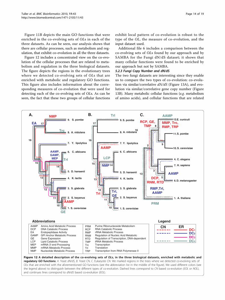
Figure 11B depicts the main GO functions that wereenriched in the co-evolving sets of OLs in each of thethree datasets. As can be seen, our analysis shows thatthere are cellular processes, such as metabolism and reg-ulation, that exhibit co-evolution in all the three datasets.Figure 12 includes a concentrated view on the co-evo-

lution of the cellular processes that are related to meta-bolism and regulation in the three biological datasets.The figure depicts the regions in the evolutionary treeswhere we detected co-evolving sets of OLs that areenriched with metabolic and regulatory GO functions.This figure also includes information about the corre-sponding measures of co-evolution that were used fordetecting each of the co-evolving sets of OLs. As can beseen, the fact that these two groups of cellular functions

exhibit local pattern of co-evolution is robust to thetype of the OL, the measure of co-evolution, and theinput dataset used.Additional file 6 includes a comparison between the

co-evolving sets of OLs found by our approach and bySAMBA for the Fungi dN/dS dataset; it shows thatmany cellular functions were found to be enriched byour approach but not by SAMBA.5.2.3 Fungi Copy Number and dN/dSThe two fungi datasets are interesting since they enableus to compare the two types of co-evolution: co-evolu-tion via similar/correlative dN/dS (Figure 13A), and evo-lution via similar/correlative gene copy number (Figure13B). Many metabolic cellular functions (e.g. metabolismof amino acids), and cellular functions that are related

S. pombe

A.

S. cerevisiae

S. bayanus

S. glabrata

K. lactis

D. hansenii

C. albicans

Y. lipolytica

A. nidulansTrc

Trl

GE

AAMP

NMP

AAMP,GAMP,MEP

EA

AbbreviationsPRMRCPRMPRNMRTDTMPTrcTrlTRP

Purine Ribonucleoside MetabolismRNA Catabolic ProcessrRNA Metabolic ProcessRegulation of Nucleic Acid MetabolicRegulation of Transcription, DNA-dependenttRNA Metabolic ProcessTranscriptionTranslationTranscription from RNA Polymerase II

AAMPDCPEAGAMPGELCPMEPMMPNMP

Amino Acid Metabolic ProcessDNA Catabolic ProcessEndopeptidase ActivityGPI Anchor Metabolic ProcessGene ExpressionLipid Catabolic ProcessmRNA 3'-end ProcessingmRNA Metabolic ProcessNucleotide Metabolic Process

DC1

DC2

DC3

DC4

Legend

ERCN

D. melanogaster

C. E. cuniculi

A. thaliana

C. elegans

H. sapiens

S. cerevisiae

S. pombe

AAMP

PRM

AAMP

RMP,Trl,AAMP

S. pombe

B.

S. cerevisiae

S. bayanus

S. glabrata

K. lactis

D. hansenii

C. albicans

Y. lipolytica

A. nidulans

r

Trl

LCP

NMP

Trl,GE

AAMP

Trl

MMP, Trc,RMP, TRP

RCP, GE,TMP

DCP,RNM, RTD

1.

2.

3.

4.

5.

6.

7.

8.

9.

10

11

12

13

1415

16

17

1.

2.

3.

4.

5.

6.

7.

8.

9.

10

11

12

13

1415

16

17

16

1.

6.

7.

4.

10.

11.

12.

5

9

313

8

2

Figure 12 A detailed description of the co-evolving sets of OLs, in the three biological datasets, enriched with metabolic andregulatory GO functions: A. Yeast dN/dS, B. Yeast CN, C. Eukaryote CN. We marked regions in the trees where we detected co-evolving sets ofOLs that are enriched with the aforementioned GO functions (see the abbreviation list in the middle of the figure). We used different colors (seethe legend above) to distinguish between the different types of co-evolution. Dashed lines correspond to CN based co-evolution (EOL or NOL),and continues lines correspond to dN/dS based co-evolution (EOL).


of 19

to regulation (e.g. translation) exhibit local co-evolution-ary patterns both via changes in copy number and viachanges in dN/dS. Though the GO enrichments thatappear in Figure 13A and in Figure 13B are similar, it isimportant to note that the OLs (and thus the co-evol-ving sets of OLs) in the two cases are completely differ-ent. This fact emphasizes the centrality of theseprocesses in the fungi evolution.One explanation of this phenomenon is the fact

that fungi datasets includes both anaerobic organisms(S. cerevisiae, S. bayanus and S. glabrata) and aerobic

organisms (A. nidulans, C. albicans, D. hansenii, K. lac-tis, and Y. lipolytica) [33]; and the switch between thesetwo types of metabolism required the co-evolution ofvarious metabolic processes.We discovered two regions where many of the fungal

genes underwent positive selection. By definition, suchregions in the evolutionary tree can not be discoveredby global clustering methods. The larger set of OLs (554orthologs) exhibits positive selection along the branch(11, 12) (see Figure 13A) probably following the wholegenome duplication event that has occurred at this

Transcription elongation factor

Transcription export

Proteasome core complex sensuEukaryota

Proteasome regulatory particle lidsubcomplex sensu Eukaryota

Mediator complex

U2 snRNP

A.

B.

SLIK SAGA-like complex

mRNA cleavage factor

Spliceosome

Toll-like Receptor Signaling

Cell Cycle: G1/S Checkpoint Regulation

Cell Cycle: G2/M Checkpoint Regulation

1. S. pombe

7. A. nidulans

5. M. grisea

2. F. graminearum

3. N. crassa

9. Y. lipolytica

10. C. albicans

11. C. hamasenii

16. K. waltii

13. A. gossypii

14. K. lactis

18. S. castellii

19. C. glabrata

20. C. bayanus21. S. mikatae

22. S. paradoxus

23. S. Cerevisiae

33

24

25

26

2728

29

30

32

15

17

12

46

8

Archeascomycota

Euascomycota

Hemiascomycota

31

P. troglodytes

C. familiaris

R. norvegicus

2.

1. H. sapiens

3. M. mulatta

4. B. Taurus

5.

7. M. musculus

6.

8

9

11

10

12

Primates

Laurasiatheria

Rodentia

Toll-like Receptor Signaling

Cell Cycle: G1/S Checkpoint Regulation

Cell Cycle: G2/M Checkpoint Regulation

IL-6 Signaling

GABA Receptor Signaling

Amyotrophic Lateral Sclerosis Signaling

TR/RXR Activation

Xenobiotic Metabolism Signaling

Figure 13 A. The complexes that exhibit relatively higher level of co-evolution in different parts of the Fungi tree. B. The pathways thatexhibit relatively higher level of co-evolution in different parts of the mammalian tree.


of 19

bifurcation [34]. This whole genome duplication eventprobably served as a driving force underlying this burstof positive selection, by relaxing the functional con-straints acting on each of the gene copies (see for exam-ple [35]). Interestingly, this branch also partites thefungi into two groups, anaerobic and aerobic, that werementioned above. This fact further supports the central-ity of metabolism in fungi evolution.Another set of OLs (11 orthologs) exhibits positive

selection along the subtree with the nodes 13, 14, and15 (see Figure 13A). The branch between nodes 13 and14, leads to a subgroup (D. hansenii and C. albicans)that evolved a modified version of the genetic code [36],and the branch between nodes 13 and 15 leads toY. lipolytica (which is a sole member in one of the threetaxonomical clusters of the Saccharomycotina [37]). Allthe results for these datasets appear in additional file 5and additional file 7.5.2.4 Eukaryote Copy NumberAs mentioned, this biological dataset gives a wider evo-lutionary view than the fungi datasets. Cellular processesthat are related to metabolism, signaling, and mRNAprocessing exhibit co-evolutionary patterns along thisdataset (see Figures 11B and 13). One striking phenom-enon is that many of these co-evolving sets (87%) exhib-ited co-evolution (according to all the measures of co-evolution) along the subtrees of the Animalia andFungi, and excluding the subtree of the Plantae (seeillustration in Figure 11C).It is possible that this result is partially related to the

fact that the analyzed subtrees of the Plantae includedonly one organism with relatively high evolutionarydistance from other organisms. However, we also foundtwo possible biological explanations for this phenom-enon: First, many gene modules changed their function-ality after the split between the Plantae and the twoother groups (Animalia and Fungi). Cases where homo-logous protein complexes in Plantae and Animalia haverather different functions were reported in the past. Forexample, the COP9 signalosome, a repressor of photo-morphogenesis in Plantae, regulates completely differentdevelopmental processes in Animalia [38,39]. Our ana-lysis, however, may suggest that this is a wide scalephenomenon.Second, it is possible that there is a relatively higher

rate of changes in the protein-protein interactions alongthe split between the Plantae and the two other groups(i.e. more pairs of protein gain/lose new interactions).Thus, these results suggest that the protein-proteininteraction network of Plantae may be relatively differ-ent from that of the other groups (see [40] for a com-parison of protein-protein interaction networks). To thebest of our knowledge, an alignment of the proteininteraction network of a plant and organisms from the

other two groups has not been performed yet. Whensuch an alignment will be performed, it will be possibleto check this hypothesis.All the results for these datasets appear in additional

files 8 and additional files 7.5.2.5 Co-Evolution of Cellular FunctionsThe functional enrichments of the co-evolving OLs canteach us about functional interdependencies betweencellular functions and about the co-evolution of cellularfunctions. We found many subtrees where sets of OLsthat are enriched with various GO functions exhibitedco-evolution. For example, Translation and Gene expres-sion exhibited a copy number based co-evolution in thefungi subtree that is under internal node 12 (Figure12B), as expected from two coordinated biological pro-cesses in charge of producing RNA or proteins from thecorresponding genes (DNA sequences).Additional cellular processes showed coordinated evo-

lution. For example, Translation and Amino acid meta-bolic process exhibited co-evolution in the Eukaryotes(Figure 12C) in the subtree that included nodes 1, 2, 3,4, 5, and 8 (as detected by copy number variations).The link between these two processes is probably notdirect. A possible explanation is that the evolution ofthe metabolism of various Amino Acids (AA) alteredthe composition of the AA pool in the fungi cell. Thesechanges were then followed by a corresponding evolu-tion of the translation machinery to cope with the newAA pool.5.2.6 Co-Evolution of Fungal complexesWe implemented our approach to find groups of com-plexes that exhibit correlative (Spearman Correlation)patterns of co-evolution along parts of the Fungi evolu-tionary tree (Figure 13A; see the Method section).To discover complexes that co-evolve with other com-

plexes in specific parts of the phylogenetic tree, wedivided the evolutionary tree into the three parts thatare marked in Figure 6C (Hemiascomycota, Euascomy-cota, and Archeascomycota). Then, we computed foreach complex the number of solutions (co-evolvinggroups) that include it in each of these three parts ofthe tree (all the results appear in additional files 9). Wefocused on complexes whose co-evolution with othercomplexes is time dependent (i.e. it is relatively higherin a narrow part of the evolutionary tree).We found that several complexes exhibit different

levels of co-evolution with other complexes along differ-ent parts of the evolutionary tree. For example, thecomplexes: Transcription elongation factor and Tran-scription export which are important for mRNA produc-tion, as well as the Proteasome core complex sensuEukaryota and Proteasome regulatory particle lid sub-complex sensu Eukaryota, in charge of protein degrada-tion, exhibit relatively higher level of co-evolution in the


of 19

subtree of the Hemiascomycota. These complexes affectgeneral protein amounts in the cell at two differentlevels, transcription (mRNA formation) and protein sta-bility (protein degradation). In the sub-tree of the Euas-comycota we see co-evolution of the Mediator complexand the U2 snRNP. These two complexes affect mRNAlevel by influencing the rate of transcription and therate of splicing, respectively. Finally, the SLIK SAGA-likecomplex, encoding a chromatin remodelling complex, aswell as the mRNA cleavage factor and the Spliceosome,involved in mRNA processing, exhibit relatively higherlevel of co-evolution in the subtree of theArcheascomycota.Notably, all the complexes whose co-evolution was

enriched in specific branches of the tree are involved inbasic gene expression processes at all possible levels(mRNA creation, stability and processing, protein crea-tion and stability). A recent work of Man and Pilpel [33]showed that differential translation efficiency of ortholo-gous genes can produce phenotypic divergence of Fungi.Our results may suggest a similar and wider picturewhere the co-evolution of various gene expression pro-cesses is involved in phenotypic divergence.5.2.7 Co-Evolution of Mammalian Signaling PathwaysSimilarly to the previous subsection, we implementedour approach to find groups of signaling pathways thatexhibit correlative (Spearman Correlation) and abso-lutely similar (L1 norm) pattern of co-evolution alongparts of the mammalian evolutionary tree (Figure 13B;see the Methods section).To discover co-evolution of specific pathways in speci-

fic parts of the phylogenetic tree, we divided the evolu-tionary tree into the three parts that are marked inFigure 6D (Rodentia, Laurasitheria, and Primates).Then, we computed for each pathway the number ofsolutions (co-evolving groups) that include that pathwayin each of these three parts of the tree (all the resultsappear in additional file 10). We focused on those sig-naling pathways whose co-evolution is time dependent(i.e. it is relatively higher in a narrow part of the evolu-tionary tree).In this case, we found that in general pathways exhibit

relatively homogenous levels of co-evolution along dif-ferent parts of the evolutionary tree. However, also inthis case, for the L1 norm, some of the pathways exhibitaccelerated levels of co-evolution in particular branches.For example, the pathways Toll-like Receptor Signaling,a pathogen-associated pattern recognition receptor, CellCycle: G1/S Checkpoint Regulation, and Cell Cycle: G2/M Checkpoint Regulation exhibit relatively higher levelsof co-evolution in the subtrees Rodentia and Laura-sitheria. Interestingly, in the latter subtree co-evolutioncan also be seen between these pathways and IL-6 Sig-naling, which plays a central role in inflammation. The

association between basic cellular checkpoints and theresponse to external insults such as pathogens is intri-guing and deserves further investigation.Finally, in the subtree of the Primates we observe co-

evolution of pathways related to neurotransmission andneuronal evolution (e.g. GABA Receptor Signaling, themain inhibitory neurotransmitter in mammalian CNS,TR/RXR Activation, related to activation of the thyroidhormone, and Amyotrophic Lateral Sclerosis Signaling, adisorder of the motor neurons).

6 ConclusionsIn this work we carried out a large-scale analysis of localco-evolution. As some of these problems are NP-hard,we suggested two heuristics for solving them. Weshowed that the different measures of co-evolution arenon-redundant. Finally, we demonstrated the biologicalsignificance of the local co-evolutionary problemsthrough the analysis of five biological datasets. The goalof this part was to demonstrate how our computationaltools can be used in practice.In the future, we intend to extend this work in four

directions. First, in this work, we showed that the localco-evolution is NP-hard when using Dc3 as measure ofco-evolution. It is important to show that detectinglocal co-evolution according to the other measures ofco-evolution is also NP-hard. Second, in this work wedescribed two heuristics for solving co-evolutionaryproblems. These heuristics gave very encouragingresults in the simulation study. However, as we believethat better algorithms are within reach, we plan tospend more time in designing faster and more accuratealgorithms for solving these problems. A related openproblem is to find approximation algorithms for sol-ving at least some of the co-evolutionary problemsmentioned.Third, in this work, we decided to demonstrate our

approach by focusing on four typical versions of theLocal Co-Evolutionary problem. However, the conceptthat was described here can be used for solving bothmore specific queries (e.g. finding co-evolving sets ofOLs along a subtree that includes at least one leaf)and more general ones (e.g. a joint analysis of dN/dSand copy number of orthologs across a phylogenetictree).Finally, generating biological inputs for local co-evolu-

tionary problems is a non-trivial task (see section 4.5and [6,14,22]) as it includes dozens of preprocessingsteps that should be performed properly. We plan touse our approach for studying co-evolution across theentire tree of life. To this end, we intend to generate thephylogenetic tree and the OLs of hundreds of organisms(Archaea, Bacteria, and Eukaryota), and to analyze thisinput by our approach.


of 19

Additional file 1: Supplementary Note. 1 Hardness Issues.Click here for file[ http://www.biomedcentral.com/content/supplementary/1471-2105-11-43-S1.PDF ]

Additional file 2: Supplementary Figure 1. The Bi-clustering problem isidentical to the Local Co-Evolution problem when the degree of thephylogenetic tree is unbounded.Click here for file[ http://www.biomedcentral.com/content/supplementary/1471-2105-11-43-S2.EPS ]

Additional file 3: Supplementary Table 1. List of Fungi complexes andthe result patterns of co-evolution for the fungal complexes.Click here for file[ http://www.biomedcentral.com/content/supplementary/1471-2105-11-43-S3.XLS ]

Additional file 4: Supplementary Table 2. The mammalian signalingpathways analyzed in this work.Click here for file[ http://www.biomedcentral.com/content/supplementary/1471-2105-11-43-S4.XLS ]

Additional file 5: Supplementary Table 3. The result patterns of co-evolution for the small fungi dN/dS dataset.Click here for file[ http://www.biomedcentral.com/content/supplementary/1471-2105-11-43-S5.XLS ]

Additional file 6: Supplementary Table 4. Comparison between ourapproach and SAMBA for the small fungi dN/dS dataset.Click here for file[ http://www.biomedcentral.com/content/supplementary/1471-2105-11-43-S6.XLS ]

Additional file 7: Supplementary Table 5. The result patterns of co-evolution for the small fungi Copy Number dataset.Click here for file[ http://www.biomedcentral.com/content/supplementary/1471-2105-11-43-S7.XLS ]

Additional file 8: Supplementary Table 6. The result patterns of co-evolution for the small Eukaryote Copy Number dataset.Click here for file[ http://www.biomedcentral.com/content/supplementary/1471-2105-11-43-S8.XLS ]

Additional file 9: Supplementary Table 7. Relative levels of co-evolution of Fungal complexes along different parts of the evolutionarytree.Click here for file[ http://www.biomedcentral.com/content/supplementary/1471-2105-11-43-S9.XLS ]

Additional file 10: Supplementary Table 8. Relative levels of co-evolution of mammalian signaling pathways along different parts of theevolutionary tree.Click here for file[ http://www.biomedcentral.com/content/supplementary/1471-2105-11-43-S10.XLS ]

AcknowledgementsT.T. was supported by the Edmond J. Safra Bioinformatics program at TelAviv University and the Yeshaya Horowitz Association through the Center forComplexity Science and was partially supported by a Koshland Scholaraward from the Weizmann Institute of Science. M.K. was supported bygrants from the Israel Science Foundation, the US-Israel Binational Fund(BSF) and the Israel Cancer Research Fund (ICRF). A preliminary version ofthis work has appeared in RECOMB-CG08.

Author details1School of Computer Science, Tel Aviv University, Tel Aviv, Israel.2Department of Molecular Microbiology and Biotechnology, Tel Aviv

University, Tel Aviv, Israel. 3Sackler School of Medicine, Tel-Aviv University, TelAviv, Israel. 4Faculty of Mathematics and Computer Science, WeizmannInstitute of Science, Rehovot, Israel.

Authors’ contributionsYF and TT participated in the design and execution of the study; TT and MKanalyzed the results; TT and MK participated in the preparation of thismanuscript. All authors read and approved the final manuscript.

Received: 2 March 2009Accepted: 22 January 2010 Published: 22 January 2010

References1. Chena Y, Dokholyan NV: The coordinated evolution of yeast proteins is

constrained by functional modularity. Trends in Genetics 2006,22(8):416-419.

2. Wall DP, Hirsh AE, Fraser HB, Kumm J, Giaever G, Eisen MB, Feldman MW:Functional Genomic Analysis of the Rate of Protein Evolution. Proc NatlAcad Sci USA 2005, 102(15):5483-5488.

3. o Rami’rez LM, Bodenreider O, Kantz N, Jordan IK: Co-evolutionary Rates ofFunctionally Related Yeast Genes. Evolutionary Bioinformatics 2006, 2295-2300.

4. Pazos F, Helmer-Citterich M, Ausiello G, Valencia A: Correlated MutationsContain Information About Protein-protein Interaction. J Mol Biol 1997,271:511-523.

5. Juan D, Pazos F, Valencia A: High-confidence prediction of globalinteractomes based on genome-wide coevolutionary networks. PNAS2008, 105(3):934-939.

6. Tuller T, Kupiec M, Ruppin E: Co-evolutionary Networks of Genes andCellular Processes Across Fungal Species. Genome Biol 2009, 10(5):R48.

7. Wu J, Kasif S, DeLisi C: Identification of functional links between genesusing phylogenetic profiles. Bioinformatics 2003, 19:1524-1530.

8. Snel B, Huynen M: Quantifying modularity in the evolution ofbiomolecular systems. Genome Res 2004, 14(3):391-397.

9. Bowers PM, Pellegrini M, Thompson MJ, Fierro J, Yeates TO, Eisenberg D:Prolinks: a database of protein functional linkages derived fromcoevolution. Genome Biology 2004, 5:R35.

10. Pazos F, Valencia A: Similarity of phylogenetic trees as indicator ofprotein-protein interaction. Protein Engineering 2001, 14(9):609-614.

11. Goh C, Bogan A, Joachimiak M, Walther D, Cohen F: Co-evolution ofproteins with their interaction partners. J Mol Biol 2000, 299(2):283-93.

12. Barker D, Page M: Predicting functional gene links using phylogenetic-statistical analysis of whole genomes. PLoS Comput Biol 2005, 1:24-31.

13. Barker D, Meade A, Page M: Constrained models of evolution lead toimproved prediction of functional linkage from correlated gain and lossof genes. Bioinformatics 2007, 23:14-20.

14. Wapinski I, Pfeffer A, Friedman N, Regev A: Natural history andevolutionary principles of gene duplication in fungi. Nature 2007,449:54-65.

15. Tuller T, Birin H, Gophna U, Kupiec M, Ruppin E: Reconstructing AncestralGene content by Co-Evolution. Genome Res 2009, 20:122-32.

16. Krylov DM, Wolf YI, Rogozin IB, Koonin EV: Gene loss, protein sequencedivergence, gene dispensability, expression level, and interactivity arecorrelated in eukaryotic evolution. Genome Res 2003, 13(10):2229-35.

17. Ober D, Harms R, Witte L, Hartmann T: Molecular evolution by change offunction. Alkaloid-specific homospermidine synthase retained allproperties of deoxyhypusine synthase except binding the eIF5Aprecursor protein. J Biol Chem 2003, 278(15):12805-12812.

18. Przytycka T, Jothi R, Aravind L, Lipman D: Differences in evolutionarypressure acting within highly conserved ortholog groups. BMC Evol Biol2008, 8(208).

19. Berbee M, Taylor J: The Mycota Berlin: Springer 2001 chap. Systematics andevolutionMcLaughlin D, McLaughlin E, Lemke P VIIB:229-245.

20. MacQueen JB: Some Methods for classification and Analysis ofMultivariate Observations. Proceedings of 5-th Berkeley Symposium onMathematical Statistics and Probability, Berkeley University of California Press1967, 1:281-297.

21. Grossmann S, Bauer S, Robinson PN, Vingron M: An Improved Statistic forDetecting Over-Represented Gene Ontology Annotations in Gene Sets.RECOMB06 2006, 85-98.

22. Tatusov RL, Fedorova ND, Jackson JD, Jacobs AR, Kiryutin B, Koonin EV,Krylov DM, Mazumder R, Mekhedov SL, Nikolskaya AN, Rao BS,


of 19

http://www.ncbi.nlm.nih.gov/pubmed/16797778?dopt=Abstract



































Smirnov S, Sverdlov AV, Vasudevan S, Wolf YI, Yi JJ, Natale DA: The COGdatabase: an updated version includes eukaryotes. BMC Bioinformatics2003, 4(41).

23. Bie TD, Cristianini N, Demuth JP, Hahn MW: CAFE: a computational toolfor the study of gene family evolution. Bioinformatics 2006,22:1269-1271.

24. Hedges SB, Chen H, Kumar S, Wang DY, Thompson AS, Watanabe H: Agenomic timescale for the origin of eukaryotes. BMC Evol Biol 2001,1(4).

25. Chenna R, Sugawara H, Koike T, Lopez R, Gibson TJ, Higgins DG,Thompson JD: Multiple sequence alignment with the Clustal series ofprograms. Nucleic Acids Res 2003, 31(13):3497-3500.

26. Pupko T, Pe’er I, Shamir R, Graur D: A fast algorithm for jointreconstruction of ancestral amino acid sequences. Mol Biol Evol 2000,17:890-896.

27. Yang Z, Nielsen R: Estimating synonymous and nonsynonymoussubstitution rates under realistic evolutionary models. Mol Biol Evol 2000,17:32-43.

28. Yang Z: PAML: a program package for phylogenetic analysis bymaximum likelihood. Comput Appl Biosci 1997, 13(5):555.

29. Tanay A, Sharan R, Shamir R: Discovering statistically significant biclustersin gene expression data. Bioinformatics 2002, 18:S136-44.

30. Cheng Y, Church G: Biclustering of expression data. Proc 8th Int Conf IntellSyst Mol Biol 2000, 93-103.

31. Benton M, PCJDonoghue: Paleontological evidence to date the tree oflife. Mol Biol Evol 2007, 24:26-53.

32. Jaccard P: The distribution of flora in the alpine zone. The New Phytologist1912, 11:37-50.

33. Man O, Pilpel Y: Differential translation efficiency of orthologous genes isinvolved in phenotypic divergence of yeast species. Nature Genetics 2007,39:415-421.

34. Wolfe K, Shields D: Molecular evidence for an ancient duplication of theentire yeast genome. Nature 1997, 387(6634):708-13.

35. Ohno S: Evolution by gene duplication New York: Springer-Verlag 1970.36. Dujon B, Sherman D, Fischer G, Durrens P, Casaregola S, Lafontaine I, de

Montigny J, Marck C, Neuve’glise C, Talla E, Goffard N, Frangeu L, Aigle M,Anthouard V, Babour A, Barbe V, Barnay S, Blanchin S, Beckerich JM,Beyne E, Bleykasten C, Boisrame’ A, Boyer J, Cattolico L, Confanioleri F, deDaruvar A, Despons L, Fabre E, Fairhead C, Ferry-Dumazet H, Groppi A,Hantraye F, Hennequin C, Jauniaux N, Joyet P, Kachouri R, Kerrest A,Koszul R, Lemaire M, Lesur I, Ma L, Muller H, Nicaud JM, Nikolski M, Oztas S,Ozier-Kalogeropoulos O, Pellenz S, Potier S, Richard GF, Straub ML, Suleau A,Swennen D, Tekaia F, We’solowski-Louvel M, Westhof E, Wirth B, Zeniou-Meyer M, Zivanovic I, Bolotin-Fukuhara M, Thierry A, Bouchier C, Caudron B,Scarpelli C, Gaillardin C, Weissenbach J, Wincker P, Souciet JL: Genomeevolution in yeasts. Nature 2004, 430:35-44.

37. Scannell D, Butler G, Wolfe K: Yeast genome evolution-the origin of thespecies. Yeast 2007, 24(11):929-942.

38. Oron E, Tuller T, Li L, Rozovsky N, Yekutieli D, Rencus-Lazar S, Segal D,Chor B, Edgar BA, Chamovitz DA: Genomic analysis of COP9 signalosomefunction in Drosophila melanogaster reveals a role in temporalregulation of gene expression. Mol Syst Biol 2007, 3:108.

39. Chamovitz D, Glickmanb M: The COP9 signalosome. Current Biol 2002,12(7):R232.

40. Singh R, Xu J, Berger B: Global alignment of multiple protein interactionnetworks with application to functional orthology detection. Proc NatlAcad Sci USA 2008, 105(35):12763-12768.

doi:10.1186/1471-2105-11-43Cite this article as: Tuller et al.: Discovering local patterns of co -evolution: computational aspects and biological examples. BMCBioinformatics 2010 11:43.

Submit your next manuscript to BioMed Centraland take full advantage of:

• Convenient online submission

• Thorough peer review

• No space constraints or color figure charges

• Immediate publication on acceptance

• Inclusion in PubMed, CAS, Scopus and Google Scholar

• Research which is freely available for redistribution

Submit your manuscript at www.biomedcentral.com/submit


of 19
































discovering local patterns of co - evolution: computational

Documents