discovering causal structure from observationscshalizi/uada/12/lectures/ch25.pdf · chapter 25...

Chapter 25

Discovering Causal Structurefrom Observations

The last few chapters have, hopefully, convinced you that when you want to do causalinference, knowing the causal graph is very helpful. We have looked at how it wouldlet us calculate the effects of actual or hypothetical manipulations of the variables inthe system. Furthermore, knowing the graph tells us about what causal effects wecan and cannot identify, and estimate, from observational data. But everything hasposited that we know the graph somehow. This chapter finally deals with where thegraph comes from.

There are fundamentally three ways to get the DAG:

• Prior knowledge

• Guessing-and-testing

• Discovery algorithms

There is only a little to say about the first, because, while it’s important, it’snot very statistical. As functioning adult human beings, you have a lot of everydaycausal knowledge, which does not disappear the moment you start doing data analy-sis. Moreover, you are the inheritor of a vast scientific tradition which has, throughpatient observation and toilsome experiments, acquired even more causal knowledge.You can and should use this. Someone’s sex or race or caste might be causes of thejob they get or their pay, but not the other way around. Running an electric cur-rent through a wire produces heat at a rate proportional to the square of the current.Malaria is due to a parasite transmitted by mosquitoes, and spraying mosquitoes withinsecticides makes the survivors more resistant to those chemicals. All of these sortsof ideas can be expressed graphically, or at least as constraints on graphs.

We can, and should, also use graphs to represent scientific ideas which are not assecure as Ohm’s law or the epidemiology of malaria. The ideas people work within areas like psychology or economics, are really quite tentative, but they are ideas

477

478 CHAPTER 25. DISCOVERING CAUSAL STRUCTURE

smoking

tar

genesstress

lungdisease

Figure 25.1: A hypothetical causal model in which smoking is associated with lungdisease, but does not cause it. Rather, both smoking and lung disease are caused bycommon genetic variants. (This idea was due to R. A. Fisher.) Smoking is also caused,in this model, by stress.

about the causal structure of parts of the world, and so graphical models are implicitin them.

All of which said, even if we think we know very well what’s going on, we willoften still want to check it, and that brings us the guess-and-test route.

25.1 Testing DAGsA graphical causal model makes two kinds of qualitative claims. One is about directcausation. If the model says X is a parent of Y , then it says that changing X willchange the (distribution of) Y . If we experiment on X (alone), moving it back andforth, and yet Y is unaltered, we know the model is wrong and can throw it out.

The other kind of claim a DAG model makes is about probabilistic conditionalindependence. If S d-separates X from Y , then X |= Y |S. If we observed X , Y and S,and see that X � |= Y |S, then we know the model is wrong and can throw it out. (More:we know that there is a path linking X and Y which isn’t blocked by S.) Thus in themodel of Figure 25.1, lungdisease |= tar|smoking. If lung disease and tar turn out tobe dependent when conditioning on smoking, the model must be wrong.

This then is the basis for the guess-and-test approach to getting the DAG:

• Start with an initial guess about the DAG.

• Deduce conditional independence relations from d-separation.

• Test these, and reject the DAG if variables which ought to be conditionallyindependent turn out to be dependent.

This is a distillation of primary-school scientific method: formulate a hypotheses (theDAG), work out what the hypothesis implies, test those predictions, reject hypothe-ses which make wrong predictions.

25.2. TESTING CONDITIONAL INDEPENDENCE 479

smoking

tar

genesstress

lungdisease

Figure 25.2: As in Figure 25.1, but now tar in the lungs does cause lung disease.

It may happen that there are only a few competing, scientifically-plausible models,and so only a few, competing DAGs. Then it is usually a good idea to focus onchecking predictions which differ between them. So in both Figure 25.1 and in Figure25.2, stress |= tar|smoking. Checking that independence thus does nothing to help usdistinguish between the two graphs. In particular, confirming that stress and tar areindependent given smoking really doesn’t give us evidence for the model from Figure25.1, since it equally follows from the other model. If we want such evidence, wehave to look for something they disagree about.

In any case, testing a DAG means testing conditional independence, so let’s turnto that next.

25.2 Testing Conditional Independence

Recall from §22.4 that conditional independence is equivalent to zero conditionalinformation: X |= Y |Z if and only if I [X ;Y |Z] = 0. In principle, this solves theproblem. In practice, estimating mutual information is non-trivial, and in particularthe sample mutual information often has a very complicated distribution. You couldalways bootstrap it, but often something more tractable is desirable. Completelygeneral conditional independence testing is actually an active area of research. Someof this work is still quite mathematical (Sriperumbudur et al., 2010), but it has alreadyled to practical tests (Székely and Rizzo, 2009; Gretton et al., 2012; Zhang et al., 2011)and no doubt more are coming soon.

If all the variables are discrete, one just has a big contingency table problem,and could use a G2 or χ 2 test. If everything is linear and multivariate Gaussian,X |= Y |Z is equivalent to zero partial correlation1. Nonlinearly, if X |= Y |Z , thenE[Y |Z] = E[Y |X ,Z], so if smoothing Y on X and Z leads to different predictionsthan just smoothing on Z , conditional independence fails. To reverse this, and gofrom E[Y |Z] = E[Y |X ,Z] to X |= Y |Z , requires the extra assumption that Y doesn’t

1Recall that the partial correlation between X and Y given Z is the correlation between X and Y , afterlinearly regressing each of them on Z separately. That is, it is the correlation of their residuals.


depend on X through its variance or any other moment. (This is weaker than thelinear-and-Gaussian assumption, of course.)

The conditional independence relation X |= Y |Z is fully equivalent to Pr (Y |X ,Z) =Pr (Y |Z). We could check this using non-parametric density estimation, though wewould have to bootstrap the distribution of the test statistic. A more automatic, ifslightly less rigorous, procedure comes from the idea mentioned in Chapter 15: IfX is in fact useless for predicting Y given Z , then an adaptive bandwidth selectionprocedure (like cross-validation) should realize that giving any finite bandwidth to Xjust leads to over-fitting. The bandwidth given to X should tend to the maximumallowed, smoothing X away altogether. This argument can be made more formal,and made into the basis of a test (Hall et al., 2004; Li and Racine, 2007).

25.3 Faithfulness and EquivalenceIn graphical models, d-separation implies conditional independence: if S blocks allpaths from U to V , then U |= V |S. To reverse this, and conclude that if U |= V |S thenS must d-separate U and V , we need an additional assumption, already referred to in§22.2, called faithfulness. More exactly, if the distribution is faithful to the graph,then if S does not d-separate U from V , U � |= V |S. The combination of faithfulnessand the Markov property means that U |= V |S if and only if S d-separates U and V .

This seems extremely promising. We can test whether U |= V |S for any sets ofvariables we like. We could in particular test whether each pair of variables is in-dependent, given all sorts of conditioning variable sets S. If we assume faithfulness,when we find that X |= Y |S, we know that S blocks all paths linking X and Y , sowe learn something about the graph. If X � |= Y |S for all S, we would seem to havelittle choice but to conclude that X and Y are directly connected. Might it not bepossible to reconstruct or discover the right DAG from knowing all the conditionalindependence and dependence relations?

This is on the right track, but too hasty. Start with just two variables:

X → Y ⇒ X � |= Y (25.1)X ← Y ⇒ X � |= Y (25.2)

With only two variables, there is only one independence (or dependence) relation toworry about, and it’s the same no matter which way the arrow points.

Similarly, consider these arrangements of three variables:

X → Y → Z (25.3)X ← Y ← Z (25.4)X ← Y → Z (25.5)X → Y ← Z (25.6)

The first two are chains, the third is a fork, the last is a collider. It is not hard to check(Exercise 1) that the first three DAGs all imply exactly the same set of conditional

25.4. CAUSAL DISCOVERY WITH KNOWN VARIABLES 481

independence relations, which are different from those implied by the fourth2.These examples illustrate a general problem. There may be multiple graphs which

imply the same independence relations, even when we assume faithfulness. When thishappens, the exact same distribution of observables can factor according to, and befaithful to, all of those graphs. The graphs are thus said to be equivalent, or Markovequivalent. Observational alone cannot distinguish between equivalent DAGs. Ex-periment can, of course — changing Y alters both X and Z in a fork, but not a chain— which shows that there really is a difference between the DAGs, just not one obser-vational data can track.

25.3.1 Partial Identification of EffectsChapters 23–24 considered the identification and estimation of causal effects underthe assumption that there was a single known graph. If there are multiple equivalentDAGs, then, as mentioned above, no amount of purely observational data can selecta single graph. Background knowledge lets us rule out some equivalent DAGs3, but itmay not narrow the set of possibilities to a single graph. How then are we to actuallydo our causal estimation?

We could just pick one of the equivalent graphs, and do all of our calculations asthough it were the only possible graph. This is often what people seem to do. Thekindest thing one can say about it is that it shows confidence; phrases like “lying byomission” also come to mind.

A more principled alternative is to admit that the uncertainty about the DAGmeans that causal effects are only partially identified. Simply put, one does the es-timation in each of the equivalent graphs, and reports the range of results4. If eachestimate is consistent, then this gives a consistent estimate of the range of possibleeffects. Because the effects are not fully identified, this range will not narrow to a sin-gle point, even in the limit of infinite data, but admitting this, rather than claiming anon-existent precision, is simple scientific honesty.

25.4 Causal Discovery with Known VariablesSection 25.1 talks about how we can test a DAG, once we have it. This lets us elimi-nate some DAGs, but still leaves mysterious where they come from in the first place.While in principle there is nothing wrong which deriving your DAG from a visionof serpents biting each others’ tails, so long as you test it, it would be nice to have asystematic way of finding good models. This is the problem of model discovery, andespecially of causal discovery.

2In all of the first three, X � |= Z but X |= Z |Y , while in the collider, X |= Z but X � |= Z |Y . Remarkablyenough, the work which introduced the notion of forks and colliders, Reichenbach (1956), missed this —he thought that X |= Z |Y in a collider as well as a fork. Arguably, this one mistake delayed the developmentof causal inference by thirty years or more.

3If we know that X , Y and Z have to be in either a chain or a fork, with Y in the middle, and we knowthat X comes before Y in time, then we can rule out the fork and the chain X ← Y → Z .

4Sometimes the different graphs will gave the same estimates of certain effects. For example, the chainX → Y → Z and the fork X ← Y → Z will agree on the effect of Y on Z .


Causal discovery is silly with just one variable, and too hard for us with just two.5With three or more variables, we have however a very basic principle. If there is

no edge between X and Y , in either direction, then X is neither Y ’s parent nor itschild. But any variable is independent of its non-descendants given its parents. Thus,for some set6 of variables S, X |= Y |S (Exercise 2). If we assume faithfulness, then theconverse holds: if X |= Y |S, then there cannot be an edge between X and Y . Thus,there is no edge between X and Y if and only if we can make X and Y independentby conditioning on some S. Said another way, there is an edge between X and Y ifand only if we cannot make the dependence between them go away, no matter whatwe condition on7.

So let’s start with three variables, X , Y and Z . By testing for independence andconditional independence, we could learn that there had to be edges between X and Yand Y and Z , but not between X and Z . But conditional independence is a symmetricrelationship, so how could we orient those edges, give them direction? Well, torehearse a point from the last section, there are only four possible directed graphscorresponding to that undirected graph:

• X → Y → Z (a chain);

• X ← Y ← Z (the other chain);

• X ← Y → Z (a fork on Y );

• X → Y ← Z ( a collision at Y )

With the fork or either chain, we have X |= Z |Y . On the other hand, with thecollider we have X � |= Z |Y . Thus X � |= Z |Y if and only if there is a collision at Y . Bytesting for this conditional dependence, we can either definitely orient the edges, orrule out an orientation. If X −Y −Z is just a subgraph of a larger graph, we can stillidentify it as a collider if X � |= Z | {Y, S} for all collections of nodes S (not including Xand Z themselves, of course).

With more nodes and edges, we can induce more orientations of edges by con-sistency with orientations we get by identifying colliders. For example, suppose weknow that X ,Y,Z is either a chain or a fork on Y . If we learn that X → Y , then thetriple cannot be a fork, and must be the chain X → Y → Z . So orienting the X −Yedge induces an orientation of the Y −Z edge. We can also sometimes orient edgesthrough background knowledge; for instance we might know that Y comes later intime than X , so if there is an edge between them it cannot run from Y to X .8 We can

5But see Janzing (2007); Hoyer et al. (2009) for some ideas on how you could do it if you’re willing tomake some extra assumptions. The basic idea of these papers is that the distribution of effects given causesshould be simpler, in some sense, than the distribution of causes given effects.

6Possibly empty: conditioning on the empty set of variables is the same as not conditioning at all.7“No causation without association”, as it were.8Some have argued, or at least entertained the idea, that the logic here is backwards: rather than order

in time constraining causal relations, causal order defines time order. (Versions of this idea are discussedby, inter alia, Russell (1927); Wiener (1961); Reichenbach (1956); Pearl (2009b); Janzing (2007) makes arelated suggestion). Arguably then using order in time to orient edges in a causal graph begs the question,or commits the fallacy of petitio principii. But of course every syllogism does, so this isn’t a distinctivelystatistical issue. (Take the classic: “All men are mortal; Socrates is a man; therefore Socrates is mortal.”


eliminate other edges based on similar sorts of background knowledge: men tend tobe heavier than women, but changing weight does not change sex, so there can’t bean edge (or even a directed path!) from weight to sex, though there could be one theother way around.

To sum up, we can rule out an edge between X and Y whenever we can makethem independent by conditioning on other variables; and when we have an X −Y −Z pattern, we can identify colliders by testing whether X and Z are dependent givenY . Having oriented the arrows going into colliders, we induce more orientations ofother edges.

Putting these three things — edge elimination by testing, collider finding, andinducing orientations — gives the most basic causal discovery procedure, the SGS(Spirtes-Glymour-Scheines) algorithm (Spirtes et al., 2001, §5.4.1, p. 82). This as-sumes:

1. The data-generating distribution has the causal Markov property on a graph G.

2. The data-generating distribution is faithful to G.

3. Every member of the population has the same distribution.

4. All relevant variables are in G.

5. There is only one graph G to which the distribution is faithful.

Abstractly, the algorithm works as follows:

• Start with a complete undirected graph on all p variables, with edges betweenall nodes.

• For each pair of variables X and Y , and each set of other variables S, see ifX |= Y |S; if so, remove the edge between X and Y .

• Find colliders by checking for conditional dependence; orient the edges of col-liders.

• Try to orient undirected edges by consistency with already-oriented edges; dothis recursively until no more edges can be oriented.

Pseudo-code is in Appendix F.Call the result of the SGS algorithm �G. If all of the assumptions above hold,

and the algorithm is correct in its guesses about when variables are conditionallyindependent, then �G = G. In practice, of course, conditional independence guessesare really statistical tests based on finite data, so we should write the output as �Gn ,to indicate that it is based on only n samples. If the conditional independence test isconsistent, then

limn→∞

Pr� �Gn �=G�= 0 (25.7)

How can we know that all men are mortal until we know about the mortality of this particular man,Socrates? Isn’t this just like asserting that tomatoes and peppers must be poisonous, because they belong tothe nightshade family of plants, all of which are poisonous?) While these philosophical issues are genuinelyfascinating, this footnote has gone on long enough, and it is time to return to the main text.


In other words, the SGS algorithm converges in probability on the correct causalstructure; it is consistent for all graphs G. Of course, at finite n, the probabilityof error — of having the wrong structure — is (generally!) not zero, but this justmeans that, like any statistical procedure, we cannot be absolutely certain that it’snot making a mistake.

One consequence of the independence tests making errors on finite data can bethat we fail to orient some edges — perhaps we missed some colliders. These unori-ented edges in �Gn can be thought of as something like a confidence region — theyhave some orientation, but multiple orientations are all compatible with the data.9As more and more edges get oriented, the confidence region shrinks.

If the fifth assumption above fails to hold, then there are multiple graphs G towhich the distribution is faithful. This is just a more complicated version of thedifficulty of distinguishing between the graphs X → Y and X ← Y . All the graphsin the equivalence class may have some arrows in common; in that case the SGSalgorithm will identify those arrows. If some edges differ in orientation across theequivalence class, SGS will not orient them, even in the limit. In terms of the previousparagraph, the confidence region never shrinks to a single point, just because thedata doesn’t provide the information needed to do this. The graph is only partiallyidentified.

If there are unmeasured relevant variables, we can get not just unoriented edges,but actually arrows pointing in both directions. This is an excellent sign that somebasic assumption is being violated.

25.4.1 The PC AlgorithmThe SGS algorithm is statistically consistent, but very computationally inefficient;the number of tests it does grows exponentially in the number of variables p. Thisis the worst-case complexity for any consistent causal-discovery procedure, but thisalgorithm just proceeds immediately to the worst case, not taking advantage of anypossible short-cuts.

Since it’s enough to find one S making X and Y independent to remove theiredge, one obvious short-cut is to do the tests in some order, and skip unnecessarytests. On the principle of doing the easy work first, the revised edge-removal stepwould look something like this:

• For each X and Y , see if X |= Y ; if so, remove their edge.

• For each X and Y which are still connected, and each third variable Z1, see ifX |= Y |Z ; if so, remove the edge between X and Y .

• For each X and Y which are still connected, and each third and fourth variablesZ1 and Z2, see if X |= Y |Z1,Z2; if so, remove their edge.

• . . .9I say “multiple orientations” rather than “all orientations”, because picking a direction for one edge

might induce an orientation for others.


• For each X and Y which are still connected, see if X |= Y | all the p − 2 othervariables; if so, remove, their edge.

If all the tests are done correctly, this will give the same result as the SGS procedure(Exercise 3). And if some of the tests give erroneous results, conditioning on a smallnumber of variables will tend to be more reliable than conditioning on more (why?).

We can be even more efficient, however. If X |= Y |S for any S at all, then X |= Y |S �,where all the variables in S � are adjacent to X or Y (or both) (Exercise 4). To see thesense of this, suppose that there is a single long directed path running from X to Y . Ifwe condition on any of the variables along the chain, we make X and Y independent,but we could always move the point where we block the chain to be either right nextto X or right next to Y . So when we are trying to remove edges and make X and Yindependent, we only need to condition on variables which are still connected to Xand Y , not ones in totally different parts of the graph.

This then gives us the PC10 algorithm (Spirtes et al. 2001, §5.4.2, pp. 84–88;see also Appendix F). It works exactly like the SGS algorithm, except for the edge-removal step, where it tries to condition on as few variables as possible (as above), andonly conditions on adjacent variables. The PC algorithm has the same assumptionsas the SGS algorithm, and the same consistency properties, but generally runs muchfaster, and does many fewer statistical tests. It should be the default algorithm forattempting causal discovery.

25.4.2 Causal Discovery with Hidden VariablesSuppose that the set of variables we measure is not causally sufficient. Could we atleast discover this? Could we possibly get hold of some of the causal relationships?Algorithms which can do this exist (e.g., the CI and FCI algorithms of Spirtes et al.(2001, ch. 6)), but they require considerably more graph-fu. (The RFCI algorithm(Colombo et al., 2012) is a modern, fast successor to FCI.) The results of these algo-rithms can succeed in removing some edges between observable variables, and defi-nitely orienting some of the remaining edges. If there are actually no latent commoncauses, they end up acting like the SGS or PC algorithms.

Partial identification of effects When all relevant variables are observed, all ef-fects are identified within one graph; partial identification happens because multiplegraphs are equivalent. When some variables are not observed, we may have to usethe identification strategies to get at the same effect. In fact, the same effect my beidentified in one graph and not identified in another, equivalent graph. This is, again,unfortunate, but when it happens it needs to be admitted.

25.4.3 On Conditional Independence TestsThe abstract algorithms for causal discovery assume the existence of consistent testsfor conditional independence. The implementations known to me mostly assumeeither that variables are discrete (so that one can basically use the χ 2 test), or that

10Peter-Clark


they are continuous, Gaussian, and linearly related (so that one can test for vanishingpartial correlations), though the pcalg package does allow users to provide theirown conditional independence tests as arguments. It bears emphasizing that theserestrictions are not essential. As soon as you have a consistent independence test,you are, in principle, in business. In particular, consistent non-parametric tests ofconditional independence would work perfectly well. An interesting example of thisis the paper by Chu and Glymour (2008), on finding causal models for the time series,assuming additive but non-linear models.

25.5 Software and ExamplesThe PC and FCI algorithms are implemented in the stand-alone Java program Tetrad(http://www.phil.cmu.edu/projects/tetrad/). They are also implementedin the pcalg package on CRAN (Kalisch et al., 2010, 2011). This package also in-cludes functions for calculating the effects of interventions from fitted graphs, as-suming linear models. The documentation for the functions is somewhat confusing;rather see Kalisch et al. (2011) for a tutorial introduction.

It’s worth going through how pcalg works11. The code is designed to take ad-vantage of the modularity and abstraction of the PC algorithm itself; it separates ac-tually finding the graph completely from performing the conditional independencetest, which is rather a function the user supplies. (Some common ones are built in.)For reasons of computational efficiency, in turn, the conditional independence testsare set up so that the user can just supply a set of sufficient statistics, rather than theraw data.

Let’s walk through an example12, using the mathmarks data set you saw in thesecond exam. There we had grades (“marks”) from 88 students in five mathematicalsubjects, algebra, analysis, mechanics, statistics and vectors. All five variables arepositively correlated with each other.

library(pcalg)library(SMPracticals)data(mathmarks)suffStat <- list(C=cor(mathmarks),n=nrow(mathmarks))pc.fit <- pc(suffStat, indepTest=gaussCItest, p=ncol(mathmarks),alpha=0.005)

This uses a Gaussian (-and-linear) test for conditional independence, gaussCItest,which is built into the pcalg package. Basically, it tests whether X |= Y |Z by testingwhether the partial correlation of X and Y given Z is close to zero. These partialcorrelations can all be calculated from the correlation matrix, so the line before cre-ates the sufficient statistics needed by gaussCItest — the matrix of correlations

11A word about installing the package: you’ll need the package Rgraphviz for drawing graphs,which is hosted not on CRAN (like pcalg) but on BioConductor. Try installing it, and its depen-dencies, before installing pcalg. See http://www.bioconductor.org/packages/2.10/bioc/readmes/Rgraphviz/README for help on installing Rgraphviz.

12After Spirtes et al. (2001, §6.12, pp. 152–154).

25.5. SOFTWARE AND EXAMPLES 487

Inferred DAG for mathmarks

mechanics

vectors

algebra

analysis

statistics

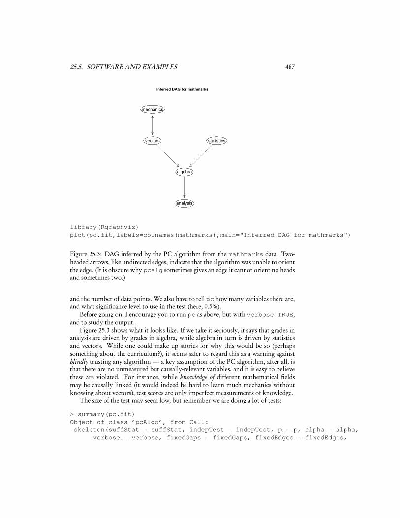
library(Rgraphviz)plot(pc.fit,labels=colnames(mathmarks),main="Inferred DAG for mathmarks")

Figure 25.3: DAG inferred by the PC algorithm from the mathmarks data. Two-headed arrows, like undirected edges, indicate that the algorithm was unable to orientthe edge. (It is obscure why pcalg sometimes gives an edge it cannot orient no headsand sometimes two.)

and the number of data points. We also have to tell pc how many variables there are,and what significance level to use in the test (here, 0.5%).

Before going on, I encourage you to run pc as above, but with verbose=TRUE,and to study the output.

Figure 25.3 shows what it looks like. If we take it seriously, it says that grades inanalysis are driven by grades in algebra, while algebra in turn is driven by statisticsand vectors. While one could make up stories for why this would be so (perhapssomething about the curriculum?), it seems safer to regard this as a warning againstblindly trusting any algorithm —- a key assumption of the PC algorithm, after all, isthat there are no unmeasured but causally-relevant variables, and it is easy to believethese are violated. For instance, while knowledge of different mathematical fieldsmay be causally linked (it would indeed be hard to learn much mechanics withoutknowing about vectors), test scores are only imperfect measurements of knowledge.

The size of the test may seem low, but remember we are doing a lot of tests:

> summary(pc.fit)Object of class ’pcAlgo’, from Call:skeleton(suffStat = suffStat, indepTest = indepTest, p = p, alpha = alpha,

verbose = verbose, fixedGaps = fixedGaps, fixedEdges = fixedEdges,


mechanics

vectors

algebra

analysis

statistics

plot(pc(suffStat, indepTest=gaussCItest, p=ncol(mathmarks),alpha=0.05),labels=colnames(mathmarks),main="")

Figure 25.4: Inferred DAG when the size of the test is 0.05.

NAdelete = NAdelete, m.max = m.max)

Nmb. edgetests during skeleton estimation:===========================================Max. order of algorithm: 3Number of edgetests from m = 0 up to m = 3 : 20 31 4 0

Graphical properties of skeleton:=================================Max. number of neighbours: 2 at node(s) 2Avg. number of neighbours: 1

This tells us that it considered going up to conditioning on three variables (the maxi-mum possible, since there are only five variables), that it did twenty tests of uncondi-tional independence, 31 tests where it conditioned on one variable, four tests whereit conditioned on two, and none where it conditioned on three. This 55 tests in all,so a simple Bonferroni correction suggests the over-all size is 55×0.005= 0.275. Thisis probably pessimistic (the Bonferroni correction typically is). Setting α= 0.05 givesa somewhat different graph (Figure 25.4).

For a second example13, let’s use some data on academic productivity among psy-

13Following Spirtes et al. (2001, §5.8.1, pp. 98–102).

25.5. SOFTWARE AND EXAMPLES 489

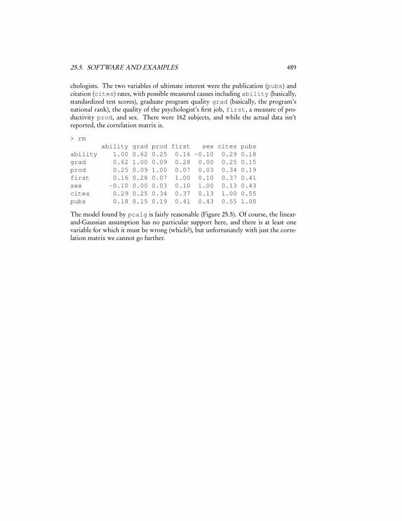
chologists. The two variables of ultimate interest were the publication (pubs) andcitation (cites) rates, with possible measured causes including ability (basically,standardized test scores), graduate program quality grad (basically, the program’snational rank), the quality of the psychologist’s first job, first, a measure of pro-ductivity prod, and sex. There were 162 subjects, and while the actual data isn’treported, the correlation matrix is.

> rmability grad prod first sex cites pubs

ability 1.00 0.62 0.25 0.16 -0.10 0.29 0.18grad 0.62 1.00 0.09 0.28 0.00 0.25 0.15prod 0.25 0.09 1.00 0.07 0.03 0.34 0.19first 0.16 0.28 0.07 1.00 0.10 0.37 0.41sex -0.10 0.00 0.03 0.10 1.00 0.13 0.43cites 0.29 0.25 0.34 0.37 0.13 1.00 0.55pubs 0.18 0.15 0.19 0.41 0.43 0.55 1.00

The model found by pcalg is fairly reasonable (Figure 25.5). Of course, the linear-and-Gaussian assumption has no particular support here, and there is at least onevariable for which it must be wrong (which?), but unfortunately with just the corre-lation matrix we cannot go further.


ability

grad prod

first sex cites

pubs

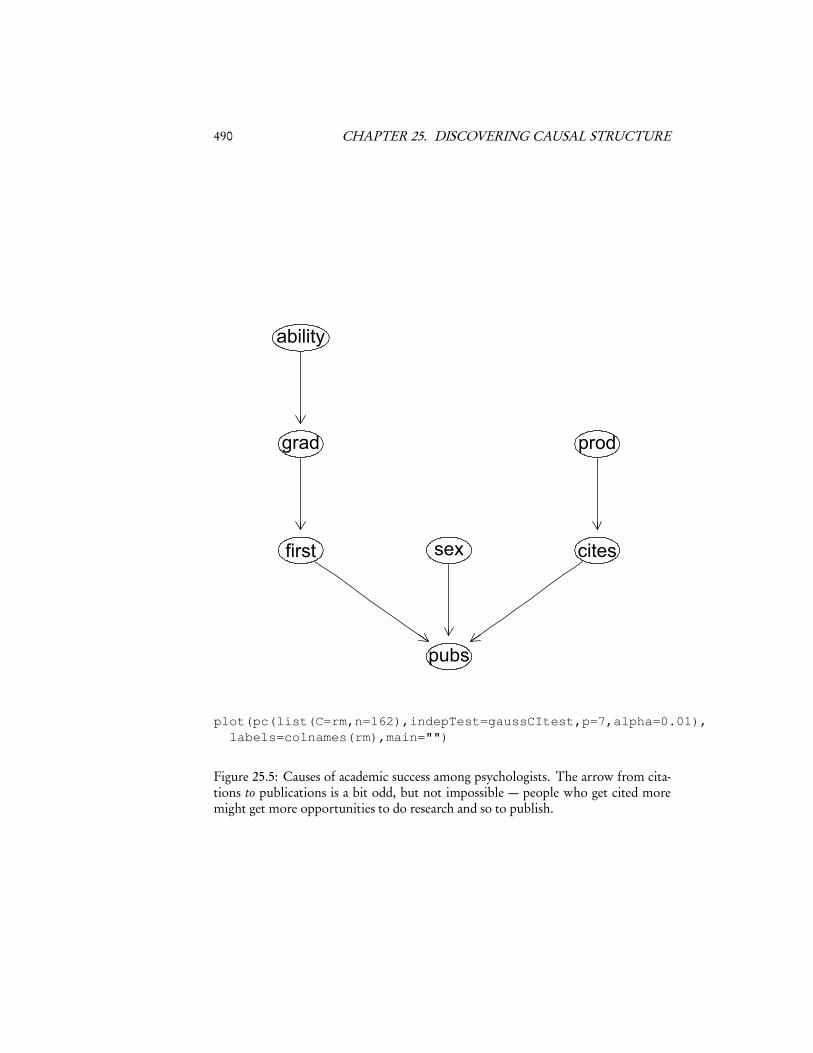
plot(pc(list(C=rm,n=162),indepTest=gaussCItest,p=7,alpha=0.01),labels=colnames(rm),main="")

Figure 25.5: Causes of academic success among psychologists. The arrow from cita-tions to publications is a bit odd, but not impossible — people who get cited moremight get more opportunities to do research and so to publish.

25.6. LIMITATIONS ON CONSISTENCY OF CAUSAL DISCOVERY 491

25.6 Limitations on Consistency of Causal DiscoveryThere are some important limitations to causal discovery algorithms (Spirtes et al.,2001, §12.4). They are universally consistent: for all causal graphs G,14

limn→∞

Pr� �Gn �=G�= 0 (25.8)

The probability of getting the graph wrong can be made arbitrarily small by usingenough data. However, this says nothing about how much data we need to achieve agiven level of confidence, i.e., the rate of convergence. Uniform consistency wouldmean that we could put a bound on the probability of error as a function of n whichdid not depend on the true graph G. Robins et al. (2003) proved that no uniformly-consistent causal discovery algorithm can exist. The issue, basically, is that the Ad-versary could make the convergence in Eq. 25.8 arbitrarily slow by selecting a distri-bution which, while faithful to G, came very close to being unfaithful, making someof the dependencies implied by the graph arbitrarily small. For any given depen-dence strength, there’s some amount of data which will let us recognize it with highconfidence, but the Adversary can make the required data size as large as he likes byweakening the dependence, without ever setting it to zero.15

The upshot is that so uniform, universal consistency is out of the question; wecan be universally consistent, but without a uniform rate of convergence; or we canconverge uniformly, but only on some less-than-universal class of distributions. Thesemight be ones where all the dependencies which do exist are not too weak (and so nottoo hard to learn reliably from data), or the number of true edges is not too large (sothat if we haven’t seen edges yet they probably don’t exist; Janzing and Herrmann,2003; Kalisch and Bühlmnann, 2007).

It’s worth emphasizing that the Robins et al. (2003) no-uniform-consistency resultapplies to any method of discovering causal structure from data. Invoking humanjudgment, Bayesian priors over causal structures, etc., etc., won’t get you out of it.

14If the true distribution is faithful to multiple graphs, then we should read G as their equivalence class,which has some undirected edges.

15Roughly speaking, if X and Y are dependent given Z , the probability of missing this conditionaldependence with a sample of size n should go to zero like O(2−nI [X ;Y |Z]), I being mutual information.To make this probability equal to, say, α we thus need n =O(− logα/I ) samples. The Adversary can thusmake n extremely large by making I very small, yet positive.


25.7 Further ReadingThe best single reference on causal discovery algorithms remains Spirtes et al. (2001).A lot of work has been done in recent years by the group centered around ETH-Zürich, beginning with Kalisch and Bühlmnann (2007), connecting this to modernstatistical concerns about sparse effects and high-dimensional data.

As already mentioned, the best reference on partial identification is Manski (2007).Partial identification of causal effects due to multiple equivalent DAGs is consideredin Maathuis et al. (2009), along with efficient algorithms for liner systems, which areapplied in Maathuis et al. (2010), and implemented in the pcalg package as ida().

Discovery is possible for directed cyclic graphs, though since it’s harder to under-stand what such models mean, it less well-developed. Important papers on this topicinclude Richardson (1996) and Lacerda et al. (2008).

25.8 ExercisesTo think through, not to hand in.

1. Prove that, assuming faithfulness, a three-variable chain and a three-variablefork imply exactly the same set of dependence and independence relations, butthat these are different from those implied by a three-variable collider. Areany implications common to chains, forks, and colliders? Could colliders bedistinguished from chains and forks without assuming faithfulness?

2. Prove that if X and Y are not parent and child, then either X |= Y , or thereexists a set of variables S such that X |= Y |S. Hint: start with the Markovproperty, that any X is independent of all its non-descendants given its parents,and consider separately the cases where Y a descendant of X and those whereit is not.

3. Prove that the graph produced by the edge-removal step of the PC algorithmis exactly the same as the graph produced by the edge-removal step of the SGSalgorithm. Hint: SGS removes the edge between X ad Y when X |= Y |S foreven one set S.

4. Prove that if X |= Y |S for some set of variables S, then X |= Y |S �, where everyvariable in S � is a neighbor of X or Y .

5. When, exactly, does E[Y |X ,Z] = E[Y |Z] imply Y |= X |Z?

6. Would the SGS algorithm work on a non-causal, merely-probabilistic DAG? Ifso, in what sense is it a causal discovery algorithm? If not, why not?

7. Describe how to use bandwidth selection as a conditional independence test.

8. Read pcalg-paper and write a conditional independence test function basedon bandwidth selection. Check that your test function gives the right sizewhen run on test cases where you know the variables are conditionally inde-pendent. Check that your test function works with pcalg::pc.

discovering causal structure from observationscshalizi/uada/12/lectures/ch25.pdf · chapter 25...

Documents