discover better designs, faster

2 Special report

2016

Discover better designs, faster.Multidisciplinary simulation and design exploration in the Oil and Gas industry.

STAR-CCM+: Discover better designs, faster. Virtual design exploration increases safety and innovation while reducing costs.

siemens.com/mdx

1 Special report

Contents

Introduction Alex Read

Engineering design in the “Lower for Longer” Environment Alex Read - Siemens PLM software

1D and 3D flow simulation helps meet deepwater flow assurance challengeDeborah Eppel - Siemens PLM software

Offshore floater design Jang Whan Kim, Hyunchul Jang and Jim O’Sullivan - Technip

Heater trouble shootingZhili (Alex) Qin - Zeeco Inc.

Prashanth Shankara - Siemens PLM software

Troubleshoot a vibrating heaterTitus sgro - Siemens PLM software

Jumper fatigue lifeOleg Voronkov, Alan Mueller, Alex Read and Sabine A. Goodwin - Siemens PLM software

Optimization of an offshore platform orientationGerard Reynolds and Andrew Staszak - Atkins

Population safety and power generationNicolas Ponchaut, Timothy Morse, Javier Castro, Gary Bigham - Exponent

Using CFD simulation to minimize risksDr Matt Straw, Norton Straw Consultants

Savvy separators - Introduction to computational fluid dynamics for separator design Alex Read - Siemens PLM software

Contents5-6

7-8

9-12

13-18

19-22

23-26

27-32

33-39

41-44

45-46

47-52

5-89-12

13-18

33-39

19-2223-26

27-3245-46

47-5241-44

2 Special report

Introduction Alex Read

3Special report

Introduction

Alex Read Introduction

The need to reduce exploration and development costs has never been more important to the future of the oil and gas industry. In addition, optimizing the through-life production efficiency and the economic extension of the life of existing and ageing fields is to key a successful future. All of this must be achieved while maintaining the highest levels of safety and environmental protection.

In oil and gas, engineering designs have traditionally been developed using empirical analysis, physical testing and experienced-based learning in the field. While these approaches remain important, the rise of simulation-based design offers engineers the opportunity to explore designs and system operation digitally through detailed, accurate prediction of a wide range of physical and chemical behavior.

Siemens’ simulation software enables engineers to explore designs digitally through detailed, accurate computational fluid dynamics (CFD) simulation and design space exploration.

Using Multiphysics simulation, it is possible to predict a wide range of physical behavior with a high-degree of fidelity in even the most complex scenarios. Multiphase flows, complex heat transfer, fluid-structure interaction and chemical reactions can all be simulated within a single, integrated

software package. In addition, automated design-space exploration enables optimized designs to be found more quickly, even when a significant number of design and operating variables exist.

In this special report we present how engineers and scientists from leading oil and gas companies are deploying Siemens’ simulation software in the design and operation of a range of oil and gas products and systems. A diverse range of applications and challenges are discussed including:

• Downhole tool optimization• Subsea and flow assurance risk reduction• Offshore and marine design• Technical safety• Process equipment design performance

Technical innovation is the key to the future of the oil and gas industry. Siemens simulation software is enabling engineers to rise to this challenge.

Alex ReadDirectorOil and Gas

4 Special report

Oil and Gas Guest Editorial

Engineering design in the“Lower for Longer” Environment

A recurring theme in the earning statements of oil and gas companies in recent months is the desire to survive not only “lower (prices) for longer,” but to usethe current market downturn, and the resulting urgency, as an opportunity to reshape organizations to ensure that they are stronger and better able to thrive in the years ahead. Clearly, the industry needs to reduce costs and continue to innovate without compromising safety, but how? In other industry crunches, such as that experienced by automotive manufacturers in 2008–09, simulation played a key role in helping to reduce engineering design costs and lead times, while allowing manufacturers to continue to deliver new and innovative solutions.

While each company’s view on how to tackle this new paradigm will differ, for many it will be to continue the day job (deliver quality and innovative products

operating conditions evaluated, and to move beyond the physical test to simulate real-world conditions at full scale, such as subsea separators with real process fluids at high temperature and pressure, or the behavior of a floating platform during a hurricane.

The importance of simulation is evident in three specific examples: two from the recent Siemens Oil, Gas, and Chemical Computational Fluid Dynamics (CFD) Conference, and one from outside our industry.

Fluid control valve (FCV) design by SchlumbergerAt the Siemens conference, Reda Bouamra of Schlumberger shared the company’s work designing downhole FCVs. Scale deposition is a significant flow assurance challenge as it can reduce production, is

Alex ReadSiemens PLM software

and solutions), but at reduced development time and cost, without compromising safety. First principles-based engineering simulation tools will be a key enabler, as companies will increasingly rely on simulation-based design exploration. The initial driver will be to reduce engineering costs and time, but companies will also benefit from simulation as an innovation enabler.

Key to this has been the rapid improvement in computer hardware and software technology, as well as innovative licensing models that enable, rather than penalize, the use of high-performance computing and cloud solutions. Through the development of cloud computing, engineers now have ready and cost-effective access to computer resources that would have been unimaginable a decade ago. These improvements allow engineers to increase the number of design and

5Special report

costly to remediate, and can cause FCVs to jam, so Schlumberger’s objective was to develop an FCV that was less susceptible to scale. Its integrated CFD-experimental design process helped the company achieve this, while reducing engineering lead times and costs. Schlumberger used CFD to design a testing program, ensuring it was as close to real well conditions as possible, and focused on the scenarios of most interest. It was able to validate CFD methods, enabling confident use of CFD to explore conditions and designs not tested.

One of the major benefits of simulation is the ease with which, having created the initial validated model, alternative designs or scenarios can be evaluated. This, plus the detailed information provided, enables engineers to come up with and efficiently test new, innovative solutions.

The industry’s move toward standardized solutions, reusable across multiple projects, introduces the need to verify equipment performance across a wide range of operating conditions. Validated simulation provides a cost-effective way to achieve this. The bottom line: An integrated CFD-experimental approach enabled Schlumberger to reduce the time and cost of the design process, while enabling evaluation of more designs in real well conditions.

Virtual wave basin at Technip Jim O’Sullivan, vice president and chief technology officer at Technip USA, explained how Technip has used a “numerical wave basin” approach on projects ranging from full-scale, vortexinduced motion of a deep draft semisubmersible to ringing on a gravity-based structure. Ringing relates to structural deflections occurring at frequencies well above incident-wave frequencies. Traditionally, the offshore sector has relied on physical testing

Guest Editorial Oil and Gas

and potential flow codes to evaluate hydrodynamic design. However, both present challenges: physical testing is expensive, timeconsuming, and results have to be translated from model to full scale. Potential flow codes omit (or have to be tuned to mimic) important physical phenomena such as viscous effects and breaking waves.

Technip also integrates CFD and physical test programs by modeling the physical test beforehand and focusing the test on the right area, reducing the chances of failure. It validates the CFD against the test, then uses CFD to explore additional designs and conditions as well as behavior at full scale under real sea conditions.

Using a validated “first principles” design tool such as CFD means results do not have to be tuned, which reduces unforeseen problems late in the design cycle or field. The bottom line: By using CFD-based design exploration, Technip is able to efficiently optimize design, using a process that better represents operating conditions, thereby reducing risk.

Evolution of simulation in the automotive industry The final example comes from outside the oil and gas industry. Whether it is a global economic crisis, new competitors entering the market, or changes in regulation, the auto industry has continually had to push to deliver innovative solutions at reduced time and cost. Those that have succeeded have done so by progressively reducing reliance on traditional methods (expensive and time-consuming physical prototyping) in favor of extensive engineering simulation.

Jaguar Land Rover (JLR) undertook a strategic shift beginning in 2008. Its goal was to not only survive an economic downturn but to significantly expand

its product offering and sales, while increasing profit. It wanted to undertake 40 “product actions” in 5 years. This is no small undertaking as today’s vehicles are highly complex with roughly 9,000 customer requirements and 3,000 assessments needed for sign-off.

The business drivers and challenges, as laid out by Andy Richardson, JLR’s head of simulation, could easily have come from an oil and gas outfit: develop new technologies while managing greatly increased system complexity; identify failure modes and establish countermeasures to achieve right first time design; reduce in-service failures; simulate the full range of use cases; and reach optimized product design efficiency and reduced production costs.

JLR is well on its way to reaching its goal of robust engineering design ready for sign-off before the first prototype is built, and it is doing so while delivering financially, with 15% or more growth in earnings before interest, taxes, depreciation, and amortization in each of the past 5 years. The bottom line: By developing a culture of simulation during lean times, driven by a need to cut costs, JLR was able to embrace the innovation potential generated by these techniques and fully capitalize on opportunities as market conditions improved.

The current “lower for longer” market conditions present significant challenges to the oil and gas industry.

For engineering design teams, it is also an opportunity to review practices and learn from others who have used downturns to reshape processes through simulation while cutting development time and costs.

Originally published in the Journal of Petroleum

Technology

“For engineering design teams, the current market is an opportunity to review practices and learn from others who have used downturns to reshape processes through simulation while cutting development time and costs.”

6 Special report

While 1D flow simulation software can accurately and rapidly simulate simple tasks, such as long straight runs, they are not adapted to complex 3D geometries such as separators, slug catchers and dry trees. Full 3D Computational Fluid Dynamics (CFD) codes, on the other hand, have the proven ability to accurately predict flow in these situations, although typically at a much higher computational cost. Generating combined 1D/3D simulations promises the best of both worlds: by making it possible to simulate complex systems of piping and equipment at a much higher level of accuracy than 1D-only simulations and in much less time than 3D-only codes, problems can be prevented earlier in the design stage.

Integration of 1D and 3D flow simulation helps meet deepwater flow assurance challenges

Deborah EppelSiemens PLM software

Below: Cooldown analysis of a subsea Christmas tree

Oil and Gas 1D and 3D flow simulation helps meet deepwater flow assurance challenge

7Special report

Above: Polyhedral mesh of a subsea Christmas tree

Flow Assurance is the ability to identify and prevent potential fluid related problems from impacting oil and gas production throughout the asset life.

1D and 3D flow simulation helps meet deepwater flow assurance challenge Oil and Gas

8 Special report

Above: Amalysis of a Y junction with two valves

AVERAGE BRENT SPOT PRICES ENERGY INFORMATION ADMINISTRATION AND BUREAU OF LABOR STATISTICS

$140

$0

MAY ‘87 JAN ‘99 JAN ‘08 JAN ‘11JUNE ‘90 JAN ‘05

REAL

NOMINAL$100

$50

Challenges of deepwater drilling and productionAs the amount of oil and gas that can easily be produced has declined, exploration and production companies have turned towards less accessible hydrocarbon sources including deepwater and ultra deepwater basins. However, the challenges associated with extracting oil and gas from such environments are considerable. To cite but a few: water depth reaching 3000 meters and beyond, higher pressures of both well fluids and ocean bottom water, high temperatures of well fluids that can run up to 300oF/150oC in near-freezing ocean water, much longer runs of

piping and risers back to production facilities and tricky ocean currents in deeper water. These difficult conditions can lead to flow assurance problems such as slugging and the formation of hydrates and waxy paraffins in an environment where remediation is far more expensive and time-consuming than in normal offshore conditions.

Advantages and limitations of 1D simulation toolsFlow assurance analysts typically use 1D modeling tools for an overall view of a field’s production scheme. 1D simulation is used for

sizing well tubing, flow lines, and receiving facilities in order to maximize the initial production while avoiding excess slugging and liquid surges later in the life of the field. Multiphase flow simulation of the well and pipeline network with a 1D code such as OLGA addresses thermal insulation and arrival temperature requirements as well as liquid inventories, flow patterns, and potential for instabilities in production systems.

In order to provide usable run times, 1D simulation has traditionally reduced 3D multiphase flow to a simplified 1D component. This requires estimating the flow regime

Oil and Gas 1D and 3D flow simulation helps meet deepwater flow assurance challenge

9Special report

Above: Flow streamlines around an oil rig

– for example stratified, annular or plug – historically accomplished by conducting expensive physical experiments to provide the 1D flow coefficients. The accuracy of the 1D simulation is thus limited by the physical conditions in which the experiment was performed; as the oil and gas industry moves to increasing depths, experiments performed at shallower depths become less and less relevant.Another concern is that the geometries of deepwater equipment often surpass the level of complexity that can be simulated using “off-the-shelf” components provided in 1D simulation tools.

Situations where the pipeline changes direction, meets up with another pipeline, or flows into a resevoir all represent inherent 3D problems. There are many others. Even in long 1D pipes, flow conditions may arise, such as recirculating flow in risers, that go beyond 1D’s predictive capabilities. In another example, gas lift is sometimes used by pumping pressurized gas through the pipe to push the water forward and prevent slugging, another inherently 3D phenomena that cannot be easily modeled with 1D codes.

Increasing need for 3D simulation 3D simulation can address these issues thanks to its ability to simulate multiphase flow in a 3D environment with no need for assumptions based on empirical data. A CFD simulation provides fluid velocity, pressure, temperature, gas composition, and other variables throughout the solution domain for problems with complex geometries and boundary conditions. As part of the analysis, an engineer may change the geometry of the system or

the boundary conditions and observe the effect of these changes on fluid flow patterns or distributions of other variables, such as gas composition.

CFD is becoming increasingly important in the deepwater environment because engineers often have no empirical data to guide them. Several obstacles, however, have prevented engineers from taking greater advantage of CFD. For example, CFD simulations for the complex geometries found in subsea drilling and production can be computationally expensive and used to take an unacceptably long period of time to solve. However, improvements in solution algorithms and the move towards massively parallel high performance computing configurations have overcome this obstacle.Another potential obstacle is that engineers want to use CFD to simulate complex subsea equipment, but want to continue handling simple geometries such as straight pipeline runs with faster 1D codes. However, with the 1D and 3D software each simulating specific sections of the fluid flow, each code becomes dependent upon the other for information such as flow velocities, flow rates, and pressures at the boundaries between 1D and 3D simulated components. In the past, this required a cumbersome process whereby the analyst moved data back and forth between 1D and 3D simulations. The analyst would first simulate the entire system in 1D while knowing that accuracy would suffer in those areas where the geometry is complex. Next, the analyst would extract flow conditions at the boundaries of the geometrically complex areas and use them as the boundary conditions for the 3D simulation. The 3D simulation would provide much greater clarity

into what is happening in the complex areas. These changes would of course affect the 1D environment and the 3D results would need to be re-entered into the 1D simulation which would be re-run. Depending on the stage in the design process and the level of accuracy needed, several more iterations of manually exchanging boundary conditions between the 1D and 3D simulations might be needed. All of these iterations would have to be repeated for every design change or new set of operating conditions.

Seamless integration between 1D and 3D simulation The recent automation of information exchange between 1D and 3D codes greatly reduces the time required to perform this type of analysis while improving the accuracy of the results by providing seamless flow of information between the two. The most prominent example is the integration of STAR-CCM+® with OLGA, a leading 1D code. The STAR-CCM+ user can run OLGA as a slave process which causes the two codes to exchange data at each time step, much more frequently than is possible using manual methods.

In a typical example, a long pipeline was modeled using OLGA while STAR-CCM+ was used to simulate the multiphase transient characteristics of the slug catcher at different flow rates and gas/liquid ratios. The analysis enabled engineers to successfully optimize the design of the slug catcher to handle the wide range of flow conditions throughout the asset life, thereby greatly reducing the risk of having to replace it at a potential cost of tens of millions of dollars.

1D and 3D flow simulation helps meet deepwater flow assurance challenge Oil and Gas

10 Special report

Oil and Gas Offshore floater design

Jang Whan Kim, Hyunchul Jang and Jim O’Sullivan Technip

A cost-effective computational tool for offshore floater design

11Special report

Figure 1: Three generations of spar platforms by Technip

Figure 2: Typical design spiral without CFD (left) and with CFD (right)

Offshore floater design Oil and Gas

IntroductionOffshore floating platforms are complex engineering systems with numerous design challenges for the engineer from the perspective of safety, reliability and longevity. Amongst their various applications, floating platforms are the lifeline of offshore Oil and Gas production, a multi-billion dollar industry with far-reaching impact around the world. These platforms are subject to extreme environments ranging from harsh waves to hurricane force winds over a long period of time and ensuring platform and occupant safety is of paramount concern to the designer. Technip is a world leader in project management, engineering and construction for the energy industry in the subsea, onshore and offshore segments. As an industry leader in offshore floating platforms, Technip is constantly innovating in the design and construction of these complex systems by taking advantage of modern design tools like numerical simulation. This article details the deployment of simulation at Technip in the design spiral for offshore platforms for cost-effective, faster and efficient design.

Offshore platform design– The challengeOf the 21 spars operating or under development, Technip claims delivery of 17. These platforms range in a water depth from 590 to 2382 meters using both dry and wet tree completions. A spar is the only inherently stable platform with a center of buoyancy above the center of gravity – it cannot flip over. There are three different

spars – a classic spar, truss spar and a cell spar (see Figure 1). The spars are typically moored with a taut or semi-taut mooring system with risers for flow of fluid from the seabed to the platform. Classic spars are fully cylindrical, truss spars have cylinders at the top and a truss at the bottom to minimize heave while cell spars consist of a number of vertical cylinders. As discussed later in this article, Technip is now extending its floater design portfolio to other platform types such as tensioned leg platforms (TLP) and semi-submersibles.

The design challenges for offshore spar platforms are many:

• Accurate knowledge of the environmental loads to be experienced by the platform

• Estimates of structural loads and dynamic motions on the platform from extreme wind, current and non-linear/random waves.

The design cycle at TechnipA typical design spiral at Technip involves hull sizing to satisfy operating, installation and transportation conditions. The design process starts with global performance analysis in extreme operating conditions. Global performance refers to motion in water, and is typically carried out by using semi-empirical potential flow based motion solvers that analytically combine gravitational and inertial forces and empirically handles rotational/viscous forces. Scale model tests are done to calibrate the global performance analysis tools, even though typically these tests properly model only the gravitational and inertial forces (Froude Number) and not the viscous forces (Reynolds Number). If the requirements of performance are not met, the entire process is carried out again before new model tests until the final performance criteria are met. Even with the long history of model tests

12 Special report

Figure 3: Typical solution from EOM – Euler solver in red, Navier Stokes in blue and overlay region in green

Figure 4: Profile of long crested wave around vertical column

Figure 5: Comparison of column moment with test data

for spars, there are always uncertainties in model testing. Furthermore, the model tests still would not completely answer questions regarding wave slamming on structures, structural resonance from wave loading, wave run-up on columns and green water on the deck (air gap).

Note that many of these design issues deal with the air-sea interface (the free surface).

The traditional design spiral at Technip involves the semi-empirical (in-house) tool called MLTSIM for the hull model to obtain hydrodynamic coefficients. An in-house catenary modeling tool, FMOOR, is used for mooring modeling and as a screening tool through a quasi-static analysis. Finally, model tests are performed to calibrate the empirical tools. Recently, CFD has been included in the design cycle to augment the design cycle and the model tests, removing much a-priori uncertainty in testing results and a-posteriori extension of modeling results once the CFD model is validated (i.e., model the model with CFD). However, due to the cost of using CFD, the semi-empirical tools, with more than 20 years of data correlation, will continue to play the main role in design iteration.

CFD will grow in acceptance doing those design simulations model tests cannot do well, or at all.

STAR-CCM+ as a Numerical wave tankTo implement numerical simulation in their design spiral, Technip uses STAR-CCM+®, a modern, fully-integrated simulation package well suited for various applications in the Oil and Gas industry. Key differentiating features of STAR-CCM+ compared to other simulation tools are the accurate capturing of the free-surface to model breaking and impact waves, motion models including Dynamic Fluid-Body Interaction (DFBI), embedded DFBI and overset mesh, and powerful pre/post processors.

One of the prohibitive factors of using CFD engineering simulation is the computational cost that is dictated by hardware resources


13Special report

Technip is constantly innovating in the design and construction of offshore floating platforms by taking advantage of modern design tools like numerical simulation.

Figure 6: Trimmed mesh on GBS (left) and wave profile around GBS (right) Figure 7: Comparison of static (black curve) and dynamic (red curve) overturning moment on GBS

available and computing time. The in-house hardware resources at Technip included a dedicated CFD cluster (144 computer cores) which can simulate 30 seconds to 1 minute of real time platform motion in less than a day. Advanced computing resources available at Texas Advanced Computing Center (TACC)comprises of more than 10,000 cores, which is 10% of the total number of cores in the Stampede cluster available through TACC’s industry partner program (STAR). Access to TACC enables multiple simulations of 3 hours of real-time motion in around a day, compared to single simulation of 30 seconds in around a day. The 3 hour period is important offshore because that is the average length of time for a storm to pass over a given location.

A typical hydrodynamic simulation of an offshore platform would require a large mesh to capture the free surface. This is accentuated when simulating for extreme environments involving violent, non-linear waves leading to higher computing time and cost. There are other gaps in the simulation methodology that also need to be addressed. Technip set out to address all the technology gaps in the existing simulation methodology with the aim of a final design tool with fully integrated CFD methodology in the design cycle.

STAR-CCM+’s Volume of Fluid (VOF) method has numerous wave models for different scenarios that have been well validated for free surface capturing. With respect to floating offshore platforms, the 5th order Stokes Wave model in STAR-CCM+ is well suited for deep water simulations which is the environment for a majority of spar

floating platforms. In the event of shallow water extreme waves, this 5th-order model is not the proper physics model. To overcome this, a fully nonlinear wave model was developed in-house for shallow water extreme waves. In addition, simulation of spar platforms required a very large domain for wave-absorbing upstream of the platform. STAR-CCM+ has a wave damping capability in the downstream direction only.

To minimize the computational cost from a very large domain, Technip developed an Euler-Overlay method where an Euler solution is used in the far-field without the hull structure and a Reynolds Averaged Navier Stokes (RANS) method with DFBI is used near the platform. An overlay method using the momentum and volume fraction sources is used at the intersection of the RANS and Euler regions to blend the two solutions smoothly. This method reduces the domain size greatly, thereby decreasing the computational time and hardware resources required by eliminating the need to solve RANS equations over a wider area.

The Euler Overlay Method (EOM) applied to real world problemsTechnip has used EOM with STAR-CCM+ successfully to provide extreme design loads on structures for a variety of offshore platforms. A proper validation of the numerical model with experimental data is the key to deciding on the appropriate numerical analysis. To validate the EOM, Technip simulated model tests from Chaplin et al. (1997) involving a long-crested wave and a vertical column. These 3D computations involved a 2m CFD domain and a 105 m long Euler solution

domain as shown in Figure 4. The moments on the column from EOM matched well with the data from model tests, thereby validating the methodology (see Figure 4).

This method was introduced in their design spiral with excellent results. A sample of how the EOM helped in the design cycle of various projects is given below:

• Ringing Analysis for Gravity-Based Spar (GBS): Ringing is a phenomenon experienced by tension leg and steel gravity-based platforms when responses of considerable amplitude are generated by these structures at their resonance period and higher harmonics, potentially causing fatigue damage over the life of the field. EOM was applied to a ringing analysis of a new Gravity-Based Platform subjected to short-crested irregular waves. Details of the trimmed hexahedral mesh around the GBS, free surface profile and the pressure profile on the structure are seen in Figure5. The 2nd order solution from EOM is obtained for a wave over a period of 15 seconds with the shortest capture period being 7.5 seconds. Model tests for this GBS were problematic with the irregular waves limiting the loading force. CFD analysis with EOM enabled proper study of this GBS at a higher loading force. Comparisons of the structural load on the spar from a static and dynamic wave are shown in the Figure 7. Numerical computations show the dynamic amplification of the structural load from the dynamic waves due to the resonant response of the structure to higher-harmonic loads.


14 Special report

Figure 8: Pressure profile on TLP with wave elevation: fixed-hull model for springing analysis

• Air Gap/Ringing Analysis of a Tensioned Leg Platform (TLP): Air gaps under an offshore platform are extremely important to consider as they determine how waves impact the underside of the structure. Technip utilized EOM for air gap and ringing analysis of a TLP. A catenary model built in STAR-CCM+ was used to simulate the tendons. The tension in the tendons reflects the ringing response and the tendon tension on the leeside and weather-side are seen in Figure 8. The numerical results agree well with model tests with the leeside tendon tension coming from the wave frequency

response and the weather-side tendon tension resulting from the natural frequency of the TLP at heave and pitch. Comparisons of air gap in the time domain with model tests also shows that CFD agrees well with model tests in predicting the air gaps and relative wave elevations.

• Semi-Submersible Motion Simulation: The EOM was used for motion analysis of a semi-submersible platform in the design phase. A mooring and riser model was used to calculate the motion of the moorings and riser. Model tests offered data on heave

response amplitude operators (RAO), an engineering statistic to determine the behavior and response of the platform in waves. Numerical analysis with the EOM model shows excellent prediction of heave RAO for the semi-submersible.

• Dry-Tree Semi-Submersible Hull Optimization: The oil and gas industry has devoted substantial efforts to find a dry tree solution for the semi-submersible in deep water with harsh environment. The key design aspect of a dry-tree Semi is to minimize heave motion to accommodate


15Special report

Figure 9: Pressure head on semi-submersible with wave elevation (top); Comparison of heave RAO from CFD and white-noise wave test (bottom)

Figure 10: Heave RAOs from CFD for several hull forms for dry-tree semi-submersibles

A

C

B

D

design limits of topsides equipment de-coupling platform motion and riser system. Technip has been developing new hull forms that suit industry demands in worldwide design environments. EOM-based CFD simulations have been used to provide heave-motion performance of the trial hull forms for the optimal dry-tree semi-submersible design.

ConclusionThe above examples show the value of simulation as an effective replacement for model tests early in the design phase to identify the more optimal offshore platform designs before moving to model tests, thereby reducing time and cost of tests and shortening the design time. CFD

can be used after model testing to extend the design into variations that shorten the overall optimization process. In addition, simulation provides more information on the physics involved compared to model tests. An example of the savings can be gathered from the total computational cost of simulations for the TLP and Semi-Submersible analysis, costing $538 and $752 respectively on 640 cores for simulating real time motion of 5 minutes and 1 hour respectively. This is a very negligible fraction of the model testing costs and overall total project costs with potential savings in design time and cost running into millions of dollars. The return on investment for simulation is extremely high for design of offshore platforms. With improved wave models and mooring/riser modeling, Technip intends to reap greater benefits from using

numerical simulation in the design cycle. The Euler Overlay Method using STAR-CCM+ has proven to be a highly useful tool for the design spiral, offering an efficient, cost-effective design process.


“The success of numerical simulation at Technip owes a lot to the very good features of STAR-CCM+ to handle analysis of platform structures”

Jang Whan KimTechnip

16 Special report

Refining and Petrochemical Heater trouble shooting

17Special report

It’s Getting Hot in Here! Zeeco solves the mystery of a heater malfunction using STAR-CCM+

STAR-CCM+ is an efficient and cost-saving engineering tool for troubleshooting

Zhili (Alex) QinZeeco Inc.

Prashanth ShankaraSiemens PLM software

IntroductionIn engineering consulting, troubleshooting the problems faced by your customer in an efficient, timely manner is the bread and butter of the business. As such, it is highly critical to be equipped with the right tools in addition to having competent engineers tackling the problem. This article showcases one such example where a modern numerical simulation software in the hands of good engineers transforms into an efficient, effective virtual troubleshooting tool.

Zeeco Inc. is a provider of combustion and environmental solutions, involved in the engineering design and manufacturing of burners, flares and incinerators. In addition, Zeeco also offers engineering consulting to their clients. One such customer came to Zeeco with a problematic heater that was suffering from low performance. This article highlights how Zeeco used, STAR-CCM+®, to virtually troubleshoot the heater and identify the cause of the heater’s inefficient operation.

Figure 1: X-cut plane section through the gear housing showing mesh details of the model

Heater trouble shooting Refining and Petrochemical

18 Special report


Figure 2: Initial distribution of the three different oil filling levels

Figure 3: Oil distribution changes in time for the middle oil level

Figure 4: (a) Streamlines showing transient flow features between the intermeshing gears and (b) transient velocity flow field changes in the gearbox

Industrial Heater – The issuesThe problematic industrial heater is shown in figure 1. The modeled system included burners on both sides at the bottom and a radiant section on top with process tubes running along the length and breadth of the heater. The convection section and stack were not included in the model. The process tubes carried processed fluids that entered the heater at the top and exited at the bottom. A combustion air distribution duct was attached to the burners to distribute the air equally to each of the burners for combustion. The walls of the heater are made of firebrick and ceramic fiber module.

The heater had the following issues while in operation and Zeeco was tasked with finding the cause and providing solutions for these: Coking: Coking is the formation of coke on the inside of the heater tubes, reducing their heat transfer capacity. The process tubes carried hydrocarbon fluid and the heavier species in the fluid were prone to coking. During operation, it was noticed that there was coking inside the process tubes. Run Length: The heater was initially designed to run for 9-10 months. Due to problems with the coking, the heater only ran for 3-4 months after which the heater had to be shut down to clean the coking inside the tubes.

Thermal Behavior: The temperature readings on the tube metal showed non-uniform temperatures and heat flux distributions at the tube surface. Visual troubleshooting of the heater and its various components is extremely difficult and impractical because there is no easy way to access to the interior of the system. Zeeco decided to turn to virtual simulation to gain insight into the heater performance. The multiphysics simulation software STAR-CCM+, was used as a troubleshooting tool for this purpose.

CFD Setup of the heaterA CAD model of the heater geometry was prepared for analysis using Solidworks. The computational model included the heater radiant section with process tubes, burners and air distribution ducts. The domain was discretized in STAR-CCM+ using trimmed hexahedral cells (figure 2) and Navier-Stokes equations were solved in these cells. Only half the heater was modeled with around 13M cells and symmetry condition was assumed for the other half. The computational mesh was refined sufficiently around the burners to resolve the flow field and combustion accurately. The heater was 85 feet long, around 25 feet tall and 10 feet wide and modeled in scale.

The segregated flow solver in STAR-CCM+ is ideally suited for low-speed flows and was used here. The fuel gas mixture in the heater

was refinery fuel gas, including hydrogen and hydrocarbons like methane and propane. STAR-CCM+offers a full suite of combustion models to simulate various combustion phenomena. The multi-component species model was used to introduce the various fuel-gas components into the heater. The Eddy Break-Up (EBU) model in STAR-CCM+ was used to model the non-premixed combustion of the species by solving the individual transport equations for mean species on the computational mesh. Ignition was not considered based on the characteristic of the heater flame and the standard EBU model was deemed sufficient to model the combustion in

conjunction with the realizable k-ε turbulence model. Radiation was accounted for by the choice of the Gray Thermal Radiation model in STAR-CCM+.

Identification of heater issues from simulationFigure 3 shows the predicted combustion flame profile depicted by iso-surfaces of the combustion output species. The combustion air enters the distribution ducts from right to left, leading to the flame height decreasing from right to left as the air available for combustion decreases. The burner at the far

19Special report


FIGURE 5: Pressure condition changes in time in the gearbox

Figure 6: Volume fraction of oil between the intermeshing gears and for the three different oil filling levels at 1/3 r (additionally for filling level high at 1/2 r)

Figure 7: a) Volume fraction of oil in the gearbox and b) on gear flanks after 1/3 r and 1 r

Figure 8: Temporal development of the volume fraction of oil on the flanks of gear 1 and gear 2

left shows anomalous behavior with higher flame length which is caused by a special duct design at the far left end. The close proximity of the flame (front view) to the side wall was confirmed by visual observation through viewing holes in the heater. Figure

4 depicts the carbon monoxide (left) and unburnt hydrocarbon (right) concentration at the central plane of each burner and shows that the CO burns out quickly, showing that completion of combustion is not an issue. Figure 5 shows the oxygen level at central

plane of each burner. Quantitative analysis of the oxygen concentration shows that excess oxygen is around 5% which is in accordance with the heater design.

The process fluid entered the heater from the top and exited at the bottom, resulting in the temperature increasing from top to bottom. A visual analysis of the tube metal temperature as seen in figure 6 confirms this behavior. Flue gas temperature at the tubes shows hot spots on the right side while the left side is cooler.

For any heater, a proper uniform distribution of heat flux at the tube surface is necessary for optimal operation. A non-uniform heat flux distribution results in poor heating and makes the hydrocarbons inside the heater prone to coking. Figure 7 shows the heat flux distribution on the tube surface. The left, right and middle sections of the heater are investigated to analyze the heat flux distribution. The weighted heat flux at various locations is compared for the three sections in plot 1. The weighted heat flux represents the ratio of the local heat flux to the overall average heat flux for all tube surfaces. It can be seen that the tube surface on the left is absorbing less heat than the surface on the right side.

Heater issues and recommendationsFor process heaters, it is very typical to see higher heat flux at lower levels where the combustion flame enters the heater as opposed to the higher elevations inside the heater where there is a lesser heat transfer and lower heat flux. From plot 1, it is apparent that at a lower elevation, the left side of the heater has a weighted heat flux of 125%, while this value jumps to 145% on the right side. This shows that the tube surface on the right side is absorbing 20% more heat than the left side, leading to coking of hydrocarbons at these higher temperatures. The heat transfer distribution on the tube surfaces is thus identified as the cause of the poor functioning of the heater. It was recommended to introduce more baffle plates and turning vanes inside the combustion air distribution duct to change the flow pattern. This will result in more uniform air distribution to all the burners, thus reducing the excessive heating of one end of the heater compared to the other.

Zeeco used STAR-CCM+ to successfully simulate the heater operation and identify the cause of the heater malfunction. Recommendations were suggested based on the numerical simulations for improved performance. STAR-CCM+ enabled Zeeco to solve an engineering challenge of a customer in a timely, cost-effective manner, reinforcing the capability of STAR-CCM+ to function as a key weapon in the arsenal of any engineering consulting organization.

20 Special report

A process heater is a direct-fired heat exchange device. It uses the hot flue gases from combustion of a commonly available fuel in a petrochemical or refinery to heat a fluid flowing through coils. These coils are placed inside the heater. The liquid inside the tubes could be crude oil, naptha, a mixture of steam and methane or others. In some cases, the heater only heats the fluid. In other cases, the the fluid may undergo high temperature reactions to produce valuable chemicals. These chemicals are further processes downstream of the heater. The processes occurring inside the tubes and the combustion occurring in the heater is a coupled phenomenon. It therefore makes these heater very complex to design and operate. Heat transfer from the burners in the heater needs to be precise to transfer enough heat without causing damage to the tubes or unwanted coking reactions inside the tubes.

The heater needs to operate safely, transfer required amount of heat and produce products in correct proportions by promoting desired reactions while minimizing pollutant gas formation such as NOx. The flow inside the coils of the heater could be multiphase or the tubes may be filled with catalysts of various shapes. This adds further complexity to the problem.

STAR-CCM+® offers a wide range of reaction and combustion models to simulate the processes in such heaters. In a new release in near future, CFD analysts will be able to couple the reaction inside the tubes with the combustion phenomenon in the heater in a seamless manner to increase the fidelity of the results. Moreover, the burner design itself can be optimized using rigorous optimization methods using the Optimate™/Optimate+™ add-on. This helps engineers in minimizing the number of experimental trials and arrive at superior designs faster.


21Special report

The bane of most engineers is dealing with physics that have not been considered during the design process and consequently troubleshooting the problem caused by it. This phenomenon is universal across the engineering world, with operating issues in equipment cropping up in countless different ways. Some unanticipated physical behavior can easily be accommodated and fixed. Others, like those often encountered by Porter McGuffie are much more difficult to diagnose and solve.

Porter McGuffie, Inc. (PMI), a Lawrence, Kansas-based computational mechanics and engineering measurement services company, provides engineering solutions backed by FEA and CFD analysis to a wide range of fields. One particular design problem they were asked to resolve was the piping inside a heater unit that was visibly and audibly shaking (and startling its operators). The cause of the shaking in the heater’s piping system (figure 1) was unknown. The oscillatory displacement was approximately one inch in each direction under certain operating conditions. This level of vibration was considered too high for safe operation. To limit the vibrations, the unit throughput had to be lowered significantly.

To begin their analysis, PMI visited the site of the heater. They attached accelerometers to the heater’s piping to get precise measurements of the vibration of the pipes. Measurements (obtained at the locations shown in figure 2) indicated that the most significant vibrations were occurring at frequencies of 10 Hz and 9 Hz, as illustrated in figure 3. Later analyses identified these

Titus SgroSiemens PLM software

Picking up Bad Vibrations: Porter McGuffie troubleshoot a vibrating heater

Figure 1: Geometry of piping, colored by sections


22 Special report

frequencies as the mechanical resonant frequencies of the two separate loops in the system. Additional analysis of the vibration data revealed that the envelope of the vibration amplitude had a periodicity to it. The primary period was approximately 27 seconds in length, and the secondary period was approximately 13.5 seconds in length, as illustrated in figure 4. This amplitude variation traded back and forth between the two loops in the heater, with one loop vibrating at ~10 HZ and then the other at ~9 Hz. This amplitude variation was nearly 180 degrees out of phase between the two loops.

Using this data, PMI was able to correlate the change in vibration levels to the flow of hydrogen in the two-phase distillate stream. To identify the cause of the change in hydrogen flow, PMI performed a CFD analysis on the heater piping system, recreating the entire flow regime in STAR-CCM+. The setup itself made use of STAR-CCM+’s Eulerian multiphase model to track the gas and liquid phase species in the pipes, as well as the S-gamma submodel to track the size of individual liquid droplets.

To enable tracking of various quantities within sections of the model, five regions were created: the inlet pipe, the convection section, cross-over section, radiant section, and the outlet tee. To accurately read the conditions of the heater, PMI set a considerable number of 3D force monitors at every elbow and pipe within the simulation as well as pressure and mass flow monitors at the entrance to each section for both liquids and gases. Flow regimes were identified within the simulation through visual inspection from still images and animations. Figure 5A shows the Fast Fourier Transform of one of the pressure graphs, with the peak period oscillations

of pressure indicated. Figure 5B shows the measured and simulated period of pressure pulses through the radiant and convection sections for each flow configuration. As is clearly shown, there is very good agreement between the simulated and measured frequency calculations, giving credence to the time-domain pressure and force traces queried from the model.

The simulation results indicated that the flow patterns in the convective region, characterized as stratified flow, did not oscillate noticeably. On the other hand, the radiative section’s flow regime showed significant annular slugging (where the liquid phase flows along the wall with a gas central core) that caused highly unstable flow patterns (figure 6). The slugging pattern that formed matched the frequency of the piping vibrations. These slug patterns also correlated with the pressure pulses measured in the radiant, cross-over, and convection sections. While this would be enough to provide good

circumstantial evidence of the cause of the shaking, Porter McGuffie was not satisfied and investigated further, coupling the STAR-CCM+ run with Algor (a finite element analysis code), using PMI proprietary coupling software. Applying the force load data from the CFD simulation, PMI was able to predict the displacement of the pipes (figure 7). The red highlights show the area in the actual heater that was having the most vibrational displacement. Figure 8 shows a comparison of the measured accelerations superimposed over the FEA-predicted accelerations, detailing obvious correlations.

Porter McGuffie was able to provide its customer with a detailed explanation of why their heater was exhibiting such high amplitude vibrations. The two-phase flow in the radiant section led to significant pressure variation in the radiative section of the simulation, which caused mass flow variations in the H2 line. The pressure variation qualitatively agreed with the

Figure 2: Locations of accelerometers on the test system

Figure 3: Vibration frequency measured at locations 9 and 10

Figure 4: Analysis to periodicity of vibrational amplitudes


23Special report

0

022

024

026

028

1

122

0 021 022 027 024 027 026 027

1722 sssssss

1624 sssssss

2227 sssssss

5555

55

5555

5

555

5

555

55 5555 55 5555 52 5255 53

)))))))))))))))))

)

))))))))

s))s))))))))s)ss))s))s))))s)))s)s)))s))s))))))))))))))

sssssssssssssssssssssssssss

ssssssssssssssssssssss

Case #Inlet

ConfigurationFlow

Configuration

Approximate Measured Period (s)

Primary CFD Calculated Period(s)

1 Reduced A/B 14,500 13.3 11

2 A/B 19,500 27 23

3 C/D 14,500 13.3 14

4 C/D 19,500 27 29

5To Exchanger

OutletA/B 19,500 27 27

7 A/B 24,500 24.5 22

8 A/B 35,000 N/A 19

hydrogen flow oscillation frequency measured on site. The force magnitudes predicted in the CFD simulation and the structural vibration analysis also lined up well with the measured data. Further experimentation and simulation have shown that while the amplitude of the flow pulsations vary with overall throughput, the frequency of the piping vibration remains constant. Again, this is in good agreement with the measured data. Thus, it is clear that a resonant mode of the piping was being excited.

PMI was able to turn around the measurements and simulations within a few weeks’ time using STAR-CCM+. The use of Eulerian Multiphase Model with S-gamma submodel allowed the analysis of a large two-phase system that took approximately one week to run using a few million cells on twelve processor cores. The more traditional Volume of Fluid model method, using the correct grid density, would have required more than 50 billion cells and weeks of run-time per simulation.

Mike Porter, principal engineer at PMI, stated that without simulation with STAR-CCM+, there would have been no way to see what the fluid flow was doing within the pipes, and it would have taken many months of analysis and research to diagnose and correct the problem. All in all, Porter McGuffie was able to do the complete testing, analysis and create a recommended redesign within the span of a few weeks, not the several months’ turn-around time common with more traditional methods and tools.

With PMI’s suggested changes scheduled to be incorporated this October, it is nearly certain that the subject heater will be able to operate at full capacity. Porter McGuffie will then maintain its record of a 100% success rate for their analysis and design solutions, a claim that most engineering companies and departments within much larger corporations can only envy.

Figure 5A: FFT of pressure from time to frequency domain

Figure 5B: Comparison of measured experimental data to CFD results

Figure 6: CFD calculated flow of liquid in the pipes, showing heavy slugging

Figure 7: CFD calculated displacement of flow pipe, accurately predicting locations of heaviest vibrations

Figure 8: Comparison of FEA-predicted accelerations and measured accelerations


24 Special report

Oil and Gas Jumper fatigue life

25Special report

Using Simulation to Assess the Fatigue Life of Subsea Jumpers

Oleg Voronkov, Alan Mueller, Alex Read and Sabine A. Goodwin Siemens PLM software

IntroductionStructural vibrations of subsea piping systems stem from either external currents passing around the structure (Vortex-Induced Vibration or VIV) or from transient flows of mixtures inside the pipes (Flow-Induced Vibration or FIV). These vibrations compromise the structural integrity of subsea systems and in extreme circumstances can reduce their fatigue life from years down to weeks.

The transient multiphase flow inside subsea piping is complex and gaining insight through physical subsea measurements is expensive and challenging. As a result of this, the industry has relied heavily on simple analysis methods to predict the effects of FIV. These approaches tend to be overly conservative, making the decision process concerning structural integrity of subsea piping systems difficult. This has had a significant economic impact on the Oil and Gas Industry as failure is not an option and thus expensive ‘over-design’ is common practice for reducing risk, with a price tag of up to hundreds of millions of dollars.

Siemens is working closely with industry to develop a set of best practices for modeling

FIV. This work describes an example of how Computational Fluid Dynamics (CFD) is being used in complement to other analysis methods by providing higher fidelity information that is otherwise unattainable, to reduce risk, reduce over-design, and increase profit margins.

Tackling the Problem of FIV with simulation Siemens is a member of a Joint Industry Programme (JIP) run by the international energy consultancy Xodus Group and the Dutch innovation company TNO to establish and validate best practices for FIV. The ultimate goal of the JIP is to contribute to industrial capability of determining the likelihood of piping fatigue due to excitation from multiphase flow. Potential benefits could include improving screening, simulation and prediction models through the use of CFD and empirical methods. [1]

This work is a demonstration example of slug flow in a jumper, modeled with two-way fully-coupled Fluid Structure Interaction (FSI). The simulations were carried out on a generic geometry of a jumper [3], to make it publicly available to Siemens' customers.

The multiphase flow encountered in jumpers covers the complete flow map including slug, annular, dispersed, stratified and wavy flow. For simulation of FIV, it is critical that the movement of the interfaces between different phases in the pipes is accurately captured and thus a multiphase model is required. The Volume of Fluid (VOF) multiphase model available in STAR-CCM+® was used to simulate the transient behavior of the mixture and the development of slugs in the jumper. VOF uses the Eulerian framework and is a practical approach for applications containing two or more immiscible fluid phases, where each phase constitutes a large structure in the system.

A key objective of this work was to address the need to understand the role FSI plays in the fatigue life of subsea structures. The dynamic open architecture in STAR-CCM+ makes it well-suited to help provide answers because it seamlessly enables FSI simulations ranging from one-way coupling of either FIV or VIV all the way up to two-way coupling, including both the internal mixture and external flow of the pipes.

The focus of the simulation work presented here is on FIV using co-simulation (fully-

Jumper fatigue life Oil and Gas

26 Special report

Figure 1: Jumper geometry in the shape of an M with a circular cross section for FSI co-simulation

Figure 2: VOF mesh generated using the generalized cylinder mesher in STAR-CCM+

The dynamic open architecture in STAR-CCM+ seamlessly enables FSI simulations ranging from one-way coupling of either FIV or VIV all the way up to two-way coupling, including both the internal mixture and external flow of the pipes.


coupled two-way interaction), where STAR-CCM+ handles the multiphase flow and Abaqus FEA (SIMULIA) is used for predicting the dynamic structural deformations of the jumper. The two domains are interconnected using the SIMULIA Co-Simulation Engine (CSE). Although this method is computationally intensive, it demonstrates a more general approach to the end user because it can be deployed for predicting the behavior of complex systems including non-linear structures and highly complicated geometries. Alternatively, because the specific generic jumper geometry for this work is geometrically and structurally relatively uncomplicated (e.g. there is no contact with the sea floor), this particular simulation could also be performed with a simpler approach by, for example, modeling the jumper with beam elements, using 1-way coupling or completely performing the FSI problem in STAR-CCM+ using its structural stress analysis model.

In addition to direct co-simulation coupling with Abaqus, STAR-CCM+ also offers users

the ability to customize their FSI simulations by leveraging the power of JAVA to allow them to easily integrate their own legacy codes or their FEA software of choice for FSI simulations.

Computational Jumper Geometry The generic jumper geometry (figure 1) in this study is made of steel, with a circular cross section and a traditional M-shape [3]. The jumper is clamped on both ends and the multiphase flow passing through the pipes consists of a 50-50% volume mixture of air and water (defined as stratified flow with water on the bottom and air on top at the inlet boundary). Fluid domain (cyan in figure 1) is extended beyond the deformable structure (yellow in figure 1) to avoid influence of boundary conditions on the flow inside the jumper.

For the VOF mesh, the generalized cylinder mesher available in STAR-CCM+ was used in conjunction with the polyhedral volume mesher. This approach works well for this

particular application because the geometry consists of cylindrical sections, and the direction of the flow is parallel to the vessel wall. Using extruded prismatic cells reduces the overall cell count, ensures orthogonal cells and improves the rate of convergence. The final VOF mesh has ~4 million polyhedral cells and is depicted in figure 2.

The Abaqus finite element model for the co-simulation consists of 21,000 four-node shell elements and is shown in figure 3. First, a stand-alone structural modal analysis was performed to characterize the dynamic behavior of the structure. The stiffness in each coordinate direction was computed by applying a load to the pipe to get the resulting force-displacement relationship and an eigenvalue analysis was done to obtain the natural frequencies of the jumper. For this case, an equivalent mass representing both the mass from the flow inside the pipes (assuming a uniform mixture of air and water) and the added mass resulting from the displacement of the water surrounding the pipe was used. This added mass coefficient was taken from

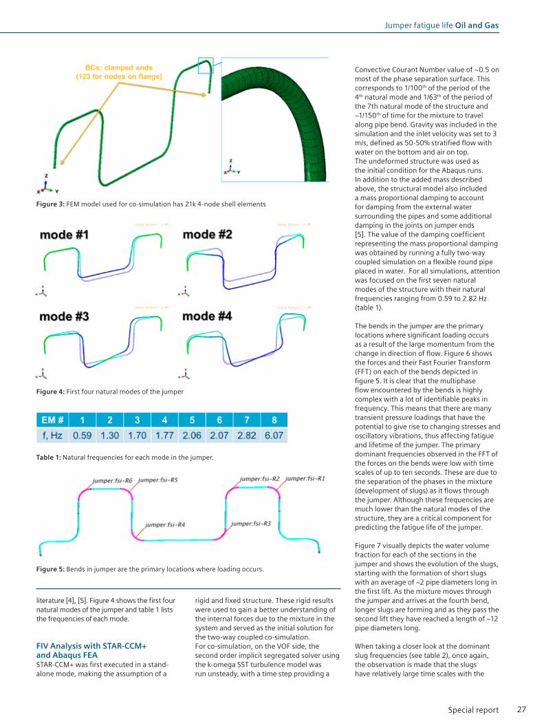
27Special report

Figure 3: FEM model used for co-simulation has 21k 4-node shell elements

Figure 4: First four natural modes of the jumper

Table 1: Natural frequencies for each mode in the jumper.

Figure 5: Bends in jumper are the primary locations where loading occurs.


literature [4], [5]. Figure 4 shows the first four natural modes of the jumper and table 1 lists the frequencies of each mode.

FIV Analysis with STAR-CCM+ and Abaqus FEASTAR-CCM+ was first executed in a stand-alone mode, making the assumption of a

rigid and fixed structure. These rigid results were used to gain a better understanding of the internal forces due to the mixture in the system and served as the initial solution for the two-way coupled co-simulation. For co-simulation, on the VOF side, the second order implicit segregated solver using the k-omega SST turbulence model was run unsteady, with a time step providing a

Convective Courant Number value of ~0.5 on most of the phase separation surface. This corresponds to 1/100th of the period of the 4th natural mode and 1/63th of the period of the 7th natural mode of the structure and ~1/150th of time for the mixture to travel along pipe bend. Gravity was included in the simulation and the inlet velocity was set to 3 m/s, defined as 50-50% stratified flow with water on the bottom and air on top. The undeformed structure was used as the initial condition for the Abaqus runs. In addition to the added mass described above, the structural model also included a mass proportional damping to account for damping from the external water surrounding the pipes and some additional damping in the joints on jumper ends [5]. The value of the damping coefficient representing the mass proportional damping was obtained by running a fully two-way coupled simulation on a flexible round pipe placed in water. For all simulations, attention was focused on the first seven natural modes of the structure with their natural frequencies ranging from 0.59 to 2.82 Hz (table 1).

The bends in the jumper are the primary locations where significant loading occurs as a result of the large momentum from the change in direction of flow. Figure 6 shows the forces and their Fast Fourier Transform (FFT) on each of the bends depicted in figure 5. It is clear that the multiphase flow encountered by the bends is highly complex with a lot of identifiable peaks in frequency. This means that there are many transient pressure loadings that have the potential to give rise to changing stresses and oscillatory vibrations, thus affecting fatigue and lifetime of the jumper. The primary dominant frequencies observed in the FFT of the forces on the bends were low with time scales of up to ten seconds. These are due to the separation of the phases in the mixture (development of slugs) as it flows through the jumper. Although these frequencies are much lower than the natural modes of the structure, they are a critical component for predicting the fatigue life of the jumper.

Figure 7 visually depicts the water volume fraction for each of the sections in the jumper and shows the evolution of the slugs, starting with the formation of short slugs with an average of ~2 pipe diameters long in the first lift. As the mixture moves through the jumper and arrives at the fourth bend, longer slugs are forming and as they pass the second lift they have reached a length of ~12 pipe diameters long.

When taking a closer look at the dominant slug frequencies (see table 2), once again, the observation is made that the slugs have relatively large time scales with the

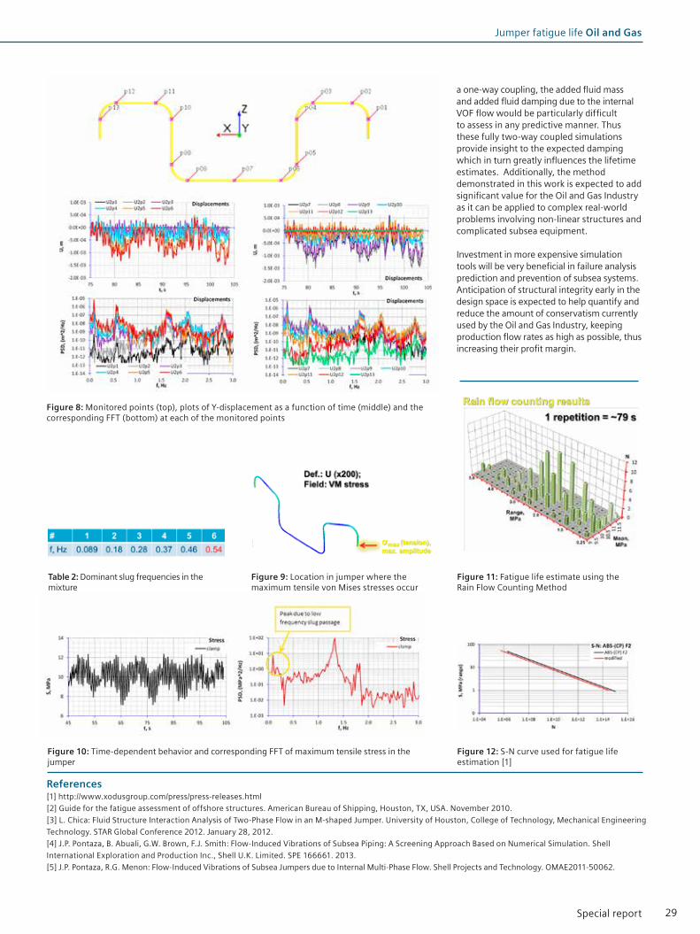
28 Special report

first dominant frequency around 0.09 Hz. Because of this, each separate slug moving along the pipe produces kind of impulse loading resulting in structural vibrations mainly with structural natural frequencies. This can be seen from the FFT of jumper displacements at controlled points (figure 8). In addition, one of the slug frequencies is observed to be close to the 1st fundamental mode of the system at 0.54 Hz (table 2).

Prediction of Fatigue FailureVon Mises stresses and displacements for the system were computed and the largest tensile stresses were observed in the cantilevered section of the pipe that is clamped in the simulation and hooks into neighboring equipment in real-life scenarios (see figure 9). This location was thus identified as a prime candidate location for prediction of fatigue failure of the jumper because usually a weld is located at this place and it is subjected to tension at this point.

The time dependent behavior of the stress at this location and its FFT are shown in figure 10. A distinct peak with a dominant frequency occurs at 1.3 Hz and falls close to the frequency of second natural mode. But in addition to this, a low frequency response of 0.09 Hz is once again present, due to the transient motion of slugs in the jumper. Using the results of the stresses at this critical location as an input, the Rain Flow Counting technique was used to estimate the damage to the jumper from the presented portion of altering stress. The result, showing range in stress relative to the mean stress and number of cycles, are depicted in figure 11. The Palmgren-Miner rule, using the S-N curve [2] shown in figure 12, predicted a short fatigue life of only about 5.5 years with a fatigue design factor of 5. This is a good example that demonstrates the value of using high-fidelity simulation to assess fatigue life early in the design process: A potential structural vibration problem is identified up front and additional simulations can be performed at a low cost to redesign the jumper and mitigate the problem.

ConclusionFlow induced vibration and its effect on fatigue life of a generic jumper was assessed using a two-way coupled FSI simulation with STAR-CCM+ and Abaqus FEA. Simulations were performed with the multiphase VOF model in STAR-CCM+ and were found to be very robust with minimal numerical problems. The dominant frequencies from the slug formation in this particular jumper geometry were much lower than the natural frequencies of the structure. This suggests that a coupling between the fluid and structure could be treated via a one-way coupling. However, for

Figure 6: Forces and their FFT on the six bends defined in the jumper geometry

Figure 7: Slug formation as the mixture travels through the jumper

Investment in more expensive simulation tools will be very beneficial in failure analysis prediction and prevention of subsea systems. Anticipation of structural integrity early in the design space is expected to help quantify and reduce the amount of conservatism currently used by the Oil and Gas Industry, keeping production flow rates as high as possible, thus increasing their profit margin.


29Special report

Figure 8: Monitored points (top), plots of Y-displacement as a function of time (middle) and the corresponding FFT (bottom) at each of the monitored points

a one-way coupling, the added fluid mass and added fluid damping due to the internal VOF flow would be particularly difficult to assess in any predictive manner. Thus these fully two-way coupled simulations provide insight to the expected damping which in turn greatly influences the lifetime estimates. Additionally, the method demonstrated in this work is expected to add significant value for the Oil and Gas Industry as it can be applied to complex real-world problems involving non-linear structures and complicated subsea equipment.

Investment in more expensive simulation tools will be very beneficial in failure analysis prediction and prevention of subsea systems. Anticipation of structural integrity early in the design space is expected to help quantify and reduce the amount of conservatism currently used by the Oil and Gas Industry, keeping production flow rates as high as possible, thus increasing their profit margin.

Table 2: Dominant slug frequencies in the mixture

Figure 9: Location in jumper where the maximum tensile von Mises stresses occur

Figure 10: Time-dependent behavior and corresponding FFT of maximum tensile stress in the jumper

Figure 11: Fatigue life estimate using the Rain Flow Counting Method

Figure 12: S-N curve used for fatigue life estimation [1]


References[1] http://www.xodusgroup.com/press/press-releases.html

[2] Guide for the fatigue assessment of offshore structures. American Bureau of Shipping, Houston, TX, USA. November 2010.

[3] L. Chica: Fluid Structure Interaction Analysis of Two-Phase Flow in an M-shaped Jumper. University of Houston, College of Technology, Mechanical Engineering

Technology. STAR Global Conference 2012. January 28, 2012.

[4] J.P. Pontaza, B. Abuali, G.W. Brown, F.J. Smith: Flow-Induced Vibrations of Subsea Piping: A Screening Approach Based on Numerical Simulation. Shell

International Exploration and Production Inc., Shell U.K. Limited. SPE 166661. 2013.

[5] J.P. Pontaza, R.G. Menon: Flow-Induced Vibrations of Subsea Jumpers due to Internal Multi-Phase Flow. Shell Projects and Technology. OMAE2011-50062.

30 Special report

Oil and Gas Optimization of an offshore platform orientation

31Special report

Optimization of an offshore platform orientation Oil and Gas

IntroductionTechnical safety in the oil and gas industry is of paramount importance. With most Tension Leg Platforms (TLP) being geographically remote, costing upwards of $3.5 billion, containing a multitude of process and operational hazards, and crowding personnel onboard, it is crucial to minimize the risks to people and assets. This can be achieved through the process of Inherently Safe Design (ISD), in which technical safety has direct influence on the design, from concept through to commissioning. The platform orientation is one design aspect that can play a significant role in the ISD process, limiting the adverse effects should an incident occur. Traditionally, the platform orientation has been determined by engineering judgment, heavily weighted by past experiences. While this approach initially appears to be cost- and time-effective, it has the potential to lead to a non-ideal design solution which could cause safety and operational issues to go unaddressed and increased costs in later design stages.

This article will discuss how the orientation and layout of an offshore platform can have a significant impact in developing a better and more informed design, keeping with the ISD principles. A case study will be discussed where STAR-CCM+® was integrated with additional analysis tools to optimize the orientation of a fixed offshore platform. It will demonstrate a technique to find the optimum platform orientation, i.e. the platform orientation which results in the best design compromise between specified parameters.

Optimization ParametersThe parameters considered for the optimization study were as follows:• The natural ventilation (wind), which

can reduce the potential accumulation of toxic and flammable gases as well as provide indications of potential vapor cloud explosion consequences.

• The helideck impairment, which can impact helicopter operations due to hot turbine exhaust gases, affecting both general operations and potential emergency operations.

• The wind chill, which can affect the ability for personnel to work on the platform. This is particularly important in cold climates and extreme weather areas where working conditions can influence the number of personnel required for operation.

• The lifeboat drift-off direction, which can impact the safety of the crew in an emergency situation.

• The hydrodynamic drag, which can affect tendon fatigue life, hull integrity, and structural design requirements.

Gerard Reynolds and Andrew StaszakAtkins

A Functional Method for the Optimization of a Tension Leg Offshore Platform Orientation Utilizing CFD

Figure 1: The aim of this study was to find the optimum theta, angle between True North and Platform North, based on a set of parameters.

32 Special report

Exhaust Outlets


Natural Ventilation (Wind)Guidance for ventilation rates is contained in the Institute of Petroleum (IP) 15 document. In the event of an unintended hydrocarbon release, higher ventilation rates typically translate into the formation of smaller flammable gas clouds. This parameter is therefore intended to be maximized.

ExhaustThe Civil Aviation Protocol (CAP) 437 dictates that restrictions be put in place to the helicopter operations if there is a temperature increase of 2 ºC above ambient within the operational zone above the helideck. Temperature rise is used to define potential impairment to operations, in some cases this may limit operations altogether or require adjustments to payload weight, approach paths, etc. For many offshore facilities, particularly in extreme weather areas, helicopters are used as the primary means of transportation and evacuation during an emergency. Thus, it is imperative that the helideck remains available through as many expected weather conditions as possible. Additionally, platforms look to minimize exhaust impacts to drilling, crane, and elevated deck operations. The helideck impairment from exhaust fumes is therefore intended to be minimized.

Wind ChillWind chill is quantified by the perceived decrease in temperature felt by the body won exposed skin and is regulated by NORSOK S-002. Wind chill can impact the number of personnel required to operate a facility. In some cases, environmental effects such as wind chill have been known to increase the potential for operator error. In order to provide personnel with acceptable working conditions and maximize safety, wind chill effects are intended to be minimized. It is important to note that this can be counter to increasing ventilation for the reduction of flammable clouds during an unintended release of hydrocarbons. One intent of the optimization approach is to find a balance between these two potentially competing goals.

Lifeboat Drift-offIf a lifeboat is deployed during an emergency, it is imperative to maximize the potential survival of the craft by limiting exposure to potential hazards. A lifeboat deployment may also suffer from loss of power, thus left to environmental effects to reach safety. To maximize the potential for survival, the lifeboat should drift safely away from the platform, assisted by the current. Adverse drift-off, the length of time to reach a safe area, and potential drift back into the

Figure 2: For a given hydrocarbon leak rate, increasing the ventilation rates aids in dispersing the flammable gas cloud, typically producing smaller explosions in case of ignition, and less probability of fatality and damage to the structure.

Figure 3: The offshore platform is powered by burning some of the gases it produces. The exhaust outlets need to be positioned in such a way that the exhaust fumes minimize potential impairment to the helideck operational zone throughout the year.

Figure 4: Wind chill index map showing the danger of frostbite to personnel

Helideck Operational Zone

33Special report


facility is intended to be minimized.Tendon StressTLP platforms are typically used in water depths reaching up to 7,000 ft. To be cost-efficient and comply with the American Petroleum Institute (API) Recommended Practice (RP) 2T, the stress in the tendons resulting from maintaining the platform in place despite wave impact and drag loading from the current needs to be minimized. Tendon requirements can lead to weight and structural design limitations, as well as require unnecessary buoyancy complications during operations.

Why Use CFD?Good judgement is fundamental in solving any engineering problem. However, numerical simulations can help in making a good design even better. In his book Expert Political Judgment: How Good is It? How Can We Know?, social scientist Philip Tetlock shows how solutions derived from formal models such as CFD consistently outperform decisions based solely on expert judgement. Today, with powerful Multidisciplinary Design Exploration (MDX) and Multidisciplinary Design Optimization (MDO) tools such as HEEDS, it has never been easier to make a design reach its best potential.

In the oil and gas industry however, decisions relating to the platform

orientation are still typically made solely based on previous experience and qualitative judgment, which can lead to unintentional biases. This study aims at improving the accuracy of experts’ predictions through the use of numerical tools in order to meet the following design objectives:• Maximize ventilation• Minimize helideck impairment from

exhaust• Minimize wind chill effects• Minimize tendon stress• Minimize adverse lifeboat drift-off

Of course, using formal models doesn’t come without limitations. There are a few challenges associated with using CFD to resolve issues related to offshore platforms:• Firstly, from a technical point of view,

offshore platforms are very large and have extremely complex geometries. This makes it difficult, if not impossible, to explicitly resolve all objects within the available time frame.

• Secondly, from a project management point of view, projects are strongly schedule-driven: stakeholders want their platform to start running as early

Figure 5: In case of emergency, lifeboats should drift away from the platform rather than into or underneath the platform.

Figure 6: With water depths reaching up to 7,000 ft, the tendon fatigue resulting from wave impact and drag loading is a significant cost factor. Here, the platform depth is compared to the height of the Burj Khalifa, which is the tallest building in the world.

Figure 7: Social scientist Philip Tetlock [1] compared 20,000 predictions made by experts in their fields with the predictions given by formal models, such as CFD. Every time, the formal models outperformed expert judgment.

34 Special report


as possible since each day of delay will cost upwards of $10 million in deferred revenue.

• In addition, the platform orientation is one of the first design aspects to be decided. However, in very early design stages, information is scarce. Many uncertainties need to be dealt with regarding the location of the equipment, etc.

• Finally, the budget allocation for Health

and Safety is usually around 1% of the total project cost, which greatly limits the amount of influence technical safety bears on the final design.

The physics parameters used in STAR-CCM+ to represent the exhaust are as follows:• Steady-state• Two-layer realizable k-epsilon turbulence

model

• Segregated multi-component gas model• Gravity model to deal with the buoyancy-

driven exhaust flowThe mesh parameters were set as follows:• Large scale objects are explicitly resolved• Small scale objects are represented by sub-

grid drag terms• Two to five million hexahedral cells• Locally refined on platform and

helideckRefined exhaust outlets

Figure 8: Mesh on the platform, showing local refinements around the exhaust outlets and the helideck

Figure 9: Mesh refinement around the exhaust outlet

35Special report


MethodologyThe methodology is summarized in the table below:

Step 1: Simulate wind from 16 direction and 2 wind speeds

Step 2: Calculate helideck impairment from exhaust for each scenario

Step 3: Calculate mean air speed through the platform

Step 4: Calculate wind chill on the platform Step 5: Determine lifeboat drift collision probability

Step 6: Calculate drag loading on hull as a surrogate for tendon stress

Step 7: Combine all results using annual wind and current probability distributions

ResultsThe cost functions for each individual design objective were calculated and are illustrated in Figures 10 to 14. Figure 15 shows the linearly weighted cost function for the combined objectives. The combined cost function shows that the optimum orientation of the platform, once all objectives are taken into account, is for its North to face True East-Southeast. This result does not coincide with any of the ideal orientations found for the individual design objectives, but is the best compromise between all these objectives.

Conclusion and future considerationsThe optimum orientation of the platform, with Platform North facing True East-Southeast, was obtained using simulation tools based on five design objectives: ventilation, exhaust, wind chill, lifeboat drift-off and tendon stress. The approach taken in this case study considers an early stage of design, with parameters covering both safety and operational issues. As the design progresses, the number of parameters considered is expected to change, as will

HOT

COLD

FAST

SLOW

36 Special report

Legend


their weighted contribution. The idea is that the orientation can be further optimized as the design process progresses or in some cases completely alter the selection based on safety and operational prioritizations. If a proper balance of previous experience, qualitative judgement, and the use of formal

models such as CFD are deployed, this function method can be used to achieve an Inherently Safe Design. Further work could involve optimizing the facility layout based on: turbine stack design and positioning, helideck positioning, module placement, flare tower design, etc.

References[1] Philip E. Tetlock: Expert Political Judgment:

How Good is It? How Can We Know?

For more information, contact

[email protected]

Figure 11: Cost function for the exhaust objective, showing that the ideal orientation from the exhaust perspective is for Platform North to be aligned with True East. However, results would be acceptable anywhere between θ = 250 and 330 degrees.

Figure 10: Cost function for the ventilation objective, showing that the ideal orientation from a ventilation perspective is for Platform North to be aligned with True North-Northwest

Figure 12: Cost function for the wind chill objective, showing that the ideal orientation from a wind chill perspective is for Platform North to be aligned with True Southeast. Note that the cost function curve is the opposite of the one obtained for the ventilation. This is explained by the fact that the wind chill is driven by the air speed in the same way as the ventilation, as well as temperature. In this specific case, the temperature was not cold enough to have much of an effect.

Figure 13: Cost function for the lifeboat drift-off objective, showing that the ideal orientation from a lifeboat drift-off perspective is for Platform North to be aligned with True South-Southeast, although any orientation θ between 180 and 260 degrees would be equally acceptable.

Figure 14: Cost function for the tendon stress objective, showing that the orientation doesn’t have any real influence on the tendon stress. This result may be explained by the symmetrical nature of the platform.

Figure 15: Cost function for all combined objectives obtained by linear weighting of the individual cost functions. It shows that the optimum platform orientation is facing True East-Southeast.

37Special report

STAR-CCM+ global academic program.Educating tomorrow's engineers today.

siemens.com/mdx

38 Special report

Nicolas Ponchaut, Timothy Morse, Javier Castro, Gary BighamExponent

Degassing Africa’s Lake Kivu for population safety and power generation

IntroductionLake Kivu is an African rift valley lake lying between Rwanda and the Democratic Republic of Congo (DRC). One of several East African rift lakes that hold high concentrations of dissolved carbon dioxide, Lake Kivu is unique in containing methane as well. The carbon dioxide comes from subaquatic springs that feed it into Lake Kivu’s deepest waters. The methane comes from bacteria decomposing organic matter at the lake bottom, from the springs, and from bacteria converting carbon dioxide into methane. The gases are kept in solution by the hydrostatic pressure in the deep waters.

This poses a danger because a landslide or volcanic activity, or even the ever-growing concentration of dissolved gases, could cause a vertical disruption of the lake water column. In such an event, also known as

a limnic eruption, gas-laden deep water is displaced to shallower depths and thus lower pressures, allowing the gas to bubble out of solution and trigger a gas eruption – an event that would imperil the lives of the more than 2 million people living along the lake’s shores.

Such an eruption happened in Cameroon twice in the 1980s. The deadlier of the two came in 1986, when a cloud of carbon dioxide erupted out of Cameroon’s Lake Nyos in a 100-meter column of water, asphyxiating more than 1,700 people as far as 25 kilometers from shore. Lake Kivu, holding one thousand times more gas than Nyos, presents an even greater danger.

But the government of Rwanda saw Lake Kivu’s methane-laden waters as not just a risk to be mitigated, but a resource to be

exploited. It approached the U.S. energy services firm ContourGlobal to design and construct a system to extract the methane and use it to greatly expand the country’s electric generating capacity, while at the same time stabilizing the lake against future overturns. The result is a 300-ton floating facility that extracts gas-laden water from deep in the lake, separates the methane and some of the carbon dioxide, then injects the degassed water back into the lake.

The $200 million KivuWatt biogas project, consisting of the gas extraction platform and an initial 25 megawatt generating plant, began operating on December 31, 2015. At its formal inauguration in May 2016, Rwandan president Paul Kagame announced the project will scale up to 100 megawatts by 2020, nearly doubling the country’s total generating capacity.

Oil and Gas Population safety and power generation

39Special report

Figure 1: KivuWatt methane extraction platform on Lake Kivu

Population safety and power generation Oil and Gas

This will be a boon to Rwanda’s economic development. Today its capital city, Kigali, is the nexus of a dynamic national economy whose yearly growth has averaged a robust eight percent over the past decade. But as the country and its capital have developed, its electricity supply has failed to keep pace. Total installed capacity before KivuWatt was only 156 megawatts. Close to 80 percent of its 12 million citizens still have no connection to the grid, and those who do have faced high electric costs because of the country’s dependence on imported diesel and heavy fuel oil to power its generators.

CFD used to analyze degassed water plume, assess risk of lake overturnAs part of the KivuWatt project, engineering and scientific consulting firm Exponent, Inc. applied computational fluid dynamics (CFD) to analyze the degassed water discharge plume from the gas extraction facility, and to characterize the dynamics of the plume. Two key concerns were raised with the degassed water plume: Could there be recirculation between the water intake risers and the degassed water discharge points? And could the dynamics of the plume lead to an overturn of the lake and a catastrophic gas eruption?

Exponent’s simulations showed that the degassed water plume ultimately stratifies within a density gradient, that recirculation does not occur, and that the discharge plume does not result in uplift or overturn of the lake for the conditions evaluated.

Characteristics of Lake KivuLake Kivu has an unusual thermal structure. At depths below approximately 80 meters, the water temperature increases with depth. However, the water also contains large quantities of dissolved carbon dioxide (CO2) and salt, with concentrations that increase with depth. The density increasing effects of CO2 and salt maintain the lake stratification despite the inverted temperature profile. The density structure of the lake is a series of relatively homogeneous mixed zones separated by density gradient layers.

The gases in Lake Kivu are kept in solution by hydrostatic pressure at depth. If a disruption to the lake due to a landslide or volcanic activity caused a parcel of gas-laden water to be brought to shallower depths where the hydrostatic pressure is below the saturation pressure (the pressure necessary to keep all the gases in solution), gas bubbles would form in the water. The bubbles would form a buoyant plume that would carry even more gas-laden water to shallower depths and release even more gases. This could

eventually result in a large-scale release of gases at the surface of the lake.

The highest concentrations of methane (CH4) in Lake Kivu are at the lowest depths, in the upper resource zone and the lower resource zone. The gas extraction facility, contained

on a floating barge, extracts gas-laden water from the lower resource zone (depth of 350 to 360 meters) through four extraction risers. The facility then separates the dissolved gases (CH4, CO2 and some H2S) from the water and re-injects the degassed water back into the lake through four discharge risers.

40 Special report

Hydrodynamic simulationsTo answer the key questions – will the degassed water recirculate back into the intake risers and prevent effective gas extraction, and will the degassed water plume upset the lake stratification and lead to a gas release – Exponent conducted several simulations of the degassed water plume using STAR-CCM+. The density of the water, and hence the plume dynamics, is heavily affected by the water temperature and by the concentration of methane, carbon dioxide and salt. Thus the computational method tracked these quantities throughout the simulation. Background conditions in the lake, including mixed zones separated by density gradients, were also included in the model.

A Reynolds-Averaged Navier Stokes (RANS) model was used, with a k-omega turbulence model. The computational domain was a cylinder with radius of 120 meters centered on the risers. The top of the domain was at a depth of 240 meters, the bottom of the domain was the lake bed at 365 meters. Pressure boundaries were used on the sides and top of the domain to allow water flow in and out of the domain. A vertical symmetry plane was applied between the two sets of intake and discharge risers. Water temperature, pressure, and species mass fractions (water, salt, CO2 and CH4) were imposed as the initial state, as well as inflow conditions on the pressure boundaries. The computational domain was discretized using a polyhedral mesh that was refined around the risers and diffusers. The simulation assumed no horizontal currents.

Plume densityThe density of the plume, both at the point of discharge and as it evolves and dilutes in the lake water, is the most important parameter that dictates the plume behavior. The density depends primarily on four variables: water temperature, salinity, concentration of CH4, and concentration of CO2. Higher temperature decreases density, while higher salinity increases density. The gas concentrations have a complicated effect on density. If the gas concentration is small enough that the local hydrostatic pressure is sufficient to hold the gases in solution, then the dissolved gases have a relatively modest (but still important) effect on the density. The presence of dissolved CO2 increases the density, while the presence of dissolved CH4 actually decreases the density.

However, if the gas concentration is high enough that the gases cannot be kept in solution by hydrostatic pressure, bubbles will form in the water, dramatically decreasing local density. Both effects – dissolved gases and gases in bubble form – must be accounted for to correctly calculate the plume density.

Figure 2: Lake Kivu, Rwanda, and location of the barge for the extraction facility

Simulated plume behaviorIn the extraction scenario that Exponent examined, raw water was extracted from a depth of 355 meters, and degassed water was reinjected at 280 meters. The four discharge risers terminated with a diffuser that directed the discharge flow horizontally. Simulation results are shown in Figures 6 to 8. To illustrate the characteristics of the discharge plume, the concentration of a passive scalar tracer (set to 1 for the degassed water discharge and 0 for the ambient lake water) is shown in Figure 6.

ConclusionIn addition to answering the critical questions, Exponent found that the degassed water plume does not enter the intake risers

but rather stratifies above them; and the dynamics of the degassed water plume do not cause uplift of the water column, so the gas extraction process does not present a risk of lake overturn, for the extraction scenario that was modeled. The simulation results also showed that the degassed water stratifies within a density gradient. This is because if the degassed water is discharged outside of a density gradient (where there is almost zero change in density with depth) and is denser than the surrounding water, there is nothing to stop the plume from sinking until it reaches a density gradient, regardless of how much mixing occurs. By adjusting the discharge depth, the degassed water plume can be controlled to stratify within any density gradient of choice.

Oil and Gas Population safety and power generation

41Special report

Figure 3: Vertical density profile in Lake Kivu, with the different zones labeled

Figure 5: Computational domain for the plume simulation

Figure 4: Diagram of the floating gas extraction barge (not to scale)

Figure 6: Passive scalar values for the degassed water plume: The four discharge risers are visible with the location of the intake points also shown. The simulation vertical symmetry plane is through the center of the image. The dark blue line shows the 95 percent dilution contour.

Population safety and power generation Oil and Gas

Figure 7: Density of the degassed water discharge plume: The dotted line indicates the simulation vertical symmetry plane.

Figure 8: Streamlines of the degassed water plume: The view is rotated 90 degrees from the view in Figures 6 and 7.

42 Special report

Oil and Gas Using CFD simulation to minimize risks

Using CFD simulation to minimize risks of hydrate formation and reduce mitigation costsDr Matt Straw Norton Straw Consulting

Deeper water, longer tieback lengths and complex production conditions continue to raise the risks of hydrate formation and costs associated with its avoidance in subsea production systems and pipelines.

Hydrate avoidance schemes usually involve a combination of thermal management and chemical injection. The latest generation of computational fluid dynamics (CFD) simulation software is providing operators and leading subsea engineering companies with a tool for reliable definition of operating strategies and effective design of insulation systems on subsea production system equipment such as Christmas trees and manifolds. CFD is able to accurately predict thermal performance of the most complex systems and now further technology development makes it possible to simulate hydrate formation mechanisms at an unprecedented level of detail.

This article will provide details on current advanced simulation techniques available to engineers designing and operating subsea production systems and also provide indications of how future technology development might change the way hydrates are managed.

Increasing risk of hydrate formation Hydrate formation can lead to serious production issues if not effectively accounted for during system design. Hydrates have the potential to rapidly form partial or even complete blockages in a system. This may lead to loss of production or even a complete shutdown. While blockages can form very quickly, the hydrate remediation process can take days or even months, resulting in high costs and significant loss of production. The technical and economic implications of hydrate remediation are high on the agenda for any exploration and production company. Current operating and shutdown strategies aim to avoid hydrate formation conditions through a combination of thermal management and chemical injection. Current

thermal management philosophies typically aim to ensure production fluids do not reach hydrate appearance temperature during operation and for a specified period following a shutdown. To deliver systems that meet this philosophy, it is important to have confidence in thermal design of the subsea production system and pipeline. This confidence can be gained either from time-consuming and expensive full-scale testing or through appropriate numerical simulation.

While 1-dimensional heat transfer calculations may be appropriate for assessing pipelines, 3-dimensional CFD simulation is the only appropriate technique for accurate thermal performance assessment of more geometrically complex pipelines (such as pipe-in-pipe, bundles), subsea production systems (Christmas trees, manifolds and connection systems) and subsea structures. CFD simulations are needed as they can account for the details of the geometry and the more complex flow and thermal behavior such as multiphase flow and natural convection. Finite element analysis (FEA) tools designed primarily to perform structural

simulations are not appropriate as they are unable to simulate the behavior of fluids explicitly, which is particularly important during cool-down, when free convection of the contained production fluid plays an important role in thermal performance.

Benefits of CFD simulation Subsea system and equipment design can make use of CFD simulations in many areas. Starting with a CAD model we can perform a wide range of simulations obtaining unparalleled detail throughout the solution domain for the most complex geometries and operating conditions. As part of a CFD simulation, an engineer may change the geometry of the system, the operating conditions or production fluids and observe the effect of the changes on such phenomena as fluid flow patterns and multiphase flow regimes as well as heat transfer rates and system temperature distributions. In addition, it is possible to predict other associated physics including sand erosion rates, fluid or chemical concentrations and even areas susceptible to internal and external corrosion.

CFD simulation of flow through subsea production system equipment

43Special report

Using CFD simulation to minimize risks Oil and Gas

Currently, CFD software can be used to obtain accurate predictions of thermal performance of the most complex systems both during production and after shutdown, as a system cools. Using the CFD approach we are able to predict exactly where and when hydrate appearance temperatures are present within a system and then use this information to modify the system or insulation design to avoid such conditions. This approach is necessary to develop a hydrate avoidance strategy that aims to maintain a system that remains completely outside of the hydrate formation zone for defined periods. It is now widely accepted that CFD can provide reliable thermal simulations to demonstrate avoidance of hydrate appearance temperatures. A number of operating subsea developments have used CFD for thermal design, some backedup by comprehensive testing programs.

Where next for flow assurance CFD simulation?Recent technology developments mean it is now possible to go further than just using CFD for thermal design where the strategy is complete avoidance of hydrate formation conditions. Computeraided engineering (CAE) software company Siemens has developed simulation techniques that incorporate multiphase flow models and the mechanisms that take place leading up to and during hydrate formation. This has been developed in its well-established STAR-CCM+® CFD software. In this approach, all production fluid phases are accounted for and, in addition, STAR-CCM+ also accounts for the temperature, pressure and chemical compositions required to simulate hydrate formation. The formation rate depends on local temperatures, pressures and fluid and phase composition. Under formation conditions the consumption of dissolved methane, required for the hydrate formation process, is simulated as a reaction process in which a fraction of free water is converted into hydrate. Not only does this method identify locations where hydrate formation conditions are present but also predicts

the location and amount of hydrate that may form in the system. This development work could lead to a step change in the way CFD simulation is used to develop subsea operating philosophies and thermal insulation designs. In the future, using CFD-based simulations, the hydrate avoidance strategy may move towards an approach where better understanding of the hydrate formation potential reduces conservatism without increasing operational and commercial risks.

Reducing time to simulation solutionsThere have been some perceived barriers to the use of detailed CFD simulation (and other 3D CAE techniques) as an integral part of the engineering process. One of the more time-consuming aspects of CFD simulation has historically been the model construction and set-up phase where we need to import CAD or build our own 3D geometrical models.

STAR-CCM+, the CFD package that Norton Straw Consultants uses for its consulting work, substantially reduces the time required to obtain simulation results. The software provides the ability to automatically import the CAD geometry from a customer’s design team. It also repairs any problems with the CAD such as surface holes or overlapping and non-manifold surfaces. This level of automation can cut geometry preparation time from weeks to days (or even hours) for the most complex subsea production system equipment and components. The software’s automatic hexahedral and polyhedral meshing tools can then produce a high-quality computational mesh, which is needed for the simulation process. Further, the ability to complete the simulation, process and assess the results, update the design and perform a revised simulation within a single software environment reduces the overall time to delivery of useful results. Setting up of parametric studies or even design optimisation studies can now become an automated process, which can add significant value to the engineering process. The continued development of parallel computing means simulations can be performed on multiple processors providing significant speed-up in simulations. This is

especially beneficial for thermal performance assessments where simulations of long cool-down events on subsea systems are common. These substantial reductions in the overall time required to perform simulations make it possible to utilize CFD to optimize subsea system designs and evaluate a wide range of operating strategies. Armed with such valuable information it is possible to identify an approach that can avoid hydrate formation in the most effective manner and at the lowest possible cost.

ConclusionHydrate risk is often regarded as the most vexing flow assurance problem in subsea production. Advanced CFD simulation can be used reliably to develop effective hydrate avoidance schemes. Furthermore, recent developments mean there is now the potential to progress towards hydrate management, through simulation of hydrate formation in the most complex production systems. Used correctly, leading edge simulation techniques can provide unparalleled engineering insight and understanding that makes it possible to develop improved subsea system designs and operating strategies that can significantly reduce the technical and commercial risks associated with flow assurance.

Production fluid temperature profiles through a subsea inline tee during operation where the main flow line is operating but the valve on the upper branch is closed leading to a cold spot around the ball valve

Contours of erosion rates on subsea component

Dr Matt Straw is a Director of Norton Straw Consultants, an engineering and technology consultancy for the oil and gas industry. He has been involved in the development and application of CFD in the oil and gas industry for 15 years and has been involved in flow assurance and thermal design of a number of major subsea developments. Using its oil and gas capability and experience in the field of fluid dynamics simulation, Norton Straw Consultants is working alongside leading simulation company Siemens providing industry-related advisory and consulting services in the development of their simulation software for the oil and gas industry.

44 Special report

OIL AND GAS GUEST EDITORIALOil and Gas Savvy separators

45Special report

Savvy separators Oil and Gas

Alex ReadSiemens PLM software

CFD for separatorsIf you work in the field of process and separation, chances are you have come across computational fluid dynamics (CFD). CFD produces a wide range of emotions ranging from abject fear, often involving flashbacks to a long forgotten university class and a dizzying array of partial-differential equations, to curiosity and even enthusiasm. The purpose of this article is to allay those fears, answer some questions and help you become an educated consumer of CFD.

Many would start by asking the “so what” question: Why and when should CFD be cared about? This question will be answered, followed by a brief introduction to CFD including the major multiphase models, answering some frequently asked questions (FAQs) and ending with a short case study example of CFD and automated design exploration being applied to a cyclone separator, all of which will be achieved without recourse to a single equation!

So why should CFD be part of the separator design?

In today’s “lower for longer” market, cost reduction is front and center for all. CFD helps in all the phases of a project: from reducing the initial project costs (CAPEX) and operating costs (OPEX) to helping manage

Savvy separators - Introduction to computational fluid dynamics for separator design

project extensions, such as tying in additional wells to an existing facility.

A subsea separator’s job is to separate gases and liquid prior to pumping. Ensuring the separator meets its process requirements is important. The pump or compressor downstream will not perform as desired if there is carry-over or under (liquid in the gas stream and gas in the liquid stream). Should this occur, operations will have a very expensive problem to resolve.

In addition to meeting the minimum process requirements, there are other design considerations. There may be a need to reduce its weight to ease installation, understand how changes in upstream piping impact performance to provide a standardized design able to connect with many Subsea Processing Systems (SPS) configurations, minimize its size to reduce the amount of real estate used, minimize the pressure drop and the use and cost of internals.

Hand calculations, such as Stokes law, can be used to estimate the required residence time, but this involves assumptions about the flow (for example, no short-circuiting or even distribution across the flow area). Physical tests can be run, however these present their own challenges: cost and time, difficulty visualizing the complex multiphase flow, testing with process fluids and high pressures

and temperatures introducing significant additional cost and safety concerns.

Using CFD, the flow patterns in upstream piping, inlet devices and within the separator can be predicted to ensure adequate residence time. Each separation mechanism can be studied such as estimating the tendency for liquid droplet re-entrainment due to high gas velocities and improving the performance of internals by increasing the uniformity of the flow to the demisters (see Dr. Lee Rhyne’s SPE webinar “CFD Optimization of Scrubber Inlet Design” for examples).

CFD achieves this with relative ease and speed, using actual process fluids, temperatures and pressures. After simulating the initial design, we can run “what-if” design studies to see how the design can be improved. In short, successful use of CFD results in discovering better designs, faster and at a lower cost.This is predicated on the assumption that the CFD study was conducted correctly, and therefore the results can be trusted. Many of the uncertainties of CFD can be systematically tested for (such as a mesh refinement study), or can be interrogated by an engineer who understands the relevant physics at hand (and not CFD). A common concern is that results must be “tuned” to be accurate. This is not necessarily the case as

46 Special report

accuracy can be obtained through systematic testing, quantification and minimization of uncertainty and error, and by ensuring the problem is adequately posed and modeling assumptions are appropriate for the problem at hand. The first step in interrogating a CFD solution is to use good engineering judgment. Does the flow field make sense, and if not, why? How does it compare with hand calculations, prior designs that have validation data and simpler analysis methods? In the early stages, CFD mistakes are often typos, so if it looks like the code solved a different problem to the one being investigated, there’s a good chance it did!

Next, it takes a deeper explanation to understand the major steps in the simulation process and the potential impact of these on the results.

CFD attempts to solve the Navier-Stokes equations which describe the behavior of fluids. Unfortunately, solving the Navier-Stokes equations is computationally intractable, so for all practical problems, the Reynolds Averaged Navier-Stokes (RANS) form is used. These suffer from the “closure problem” as they have more unknowns due to averaging which are resolved through the use of turbulence models. Models are also used to incorporate more advanced physics, such as multiphase flow dynamics. Setting up a CFD study involves four steps: 1. Defining the domain of interest, geometry,

flow entry and exit and boundary conditions (for example, velocity at the inlet)

2. Discretizing or meshing the domain: Rather than solving for the fluid behavior (velocity, pressure etc.) at every point in space, we segment the volume using a mesh, then solve the equations only at the center of each cell in the mesh - think

of a separator filled with Lego bricks. CFD will tell you what the velocity, pressure, temperature and so on, is at the center of each brick. For completeness, in time-varying problems, time is discretized by solving for time increments, such as every 0.1 seconds.

3. Selecting the physics to simulate, whether the flow is single phase or multiphase, thermal or isothermal.

4. The CFD program then iteratively solves the equations to convergence.

These steps also represent the four areas of uncertainty and where attention should be focused.

If a 3D CAD model or drawings of the geometry exist and are available, defining the domain typically is not an issue. Defining the flow conditions at the inlet and outlet is more challenging. In separator simulations it is typical to prescribe a droplet size distribution at the inlet, which requires knowing or estimating this. Typically, boundary condition information is available from other analysis methods – for example, from a 1D model of the system, from CFD by extending the domain of interest upstream to some point where there is less uncertainty or by hand calculations, for example, to estimate minimum droplet sizes. The engineer who performed the CFD study should be able to explain what conditions were used, what these mean physically and why they are appropriate.Next, the domain (geometry) needs to be discretized or meshed. This is an important and potentially time-consuming part of the analysis. A good mesh begets good CFD.

The mesh (number, size, and type of cells used) can influence the answer. As an example, if a CFD simulation is trying to

simulate a vortex using one cell, the solver only has one point at which it calculates the velocity and pressure to represent the vortex. As the number of cells is increased, decreasing the size of each cell, the resolution and therefore accuracy of the representation of the vortex improves. A similar approach is used to ensure or minimize the influence of the mesh over the solution, the mesh is progressively refined (reducing cell size) until quantities of interest, such as pressure drop, stop changing. A short note on a well-established method for grid convergence studies can be found at ¹.

There are also different cell types: hexahedral (six sides), polyhedral (many sided, but typically soccer ball shaped with 12-14 sides) or tetrahedral (four sides).

Historically, tetrahedral meshes were often used, since building hexahedral meshes was difficult and time consuming, particularly for complex geometries. This is undesirable as tetrahedral cells have poor numerical properties, they artificially make the fluid behave as if it is more viscous. As a consequence, many more tetrahedral cells are required to attain the same level of accuracy as when using hexahedral or polyhedral meshes.

Fortunately, meshing packages have improved significantly in the last decade, so it is now possible to build polyhedral or hexahedral meshes, even on complex geometries, without significant overhead. After building the mesh, the engineer must select the physics to consider. One benefit of CFD is the ability to simplify problems to consider only the physics of interest, making it easier to interrogate and understand results and trends. This is also a double-edged sword as over

Figure 1: Different cell types: tetrahedral (blue), hexahedral (green), polyhedral (red)

Oil and Gas Savvy separators

47Special report

simplifying can miss important effects. As with boundary condition selection, the engineer performing the analysis should be able to explain the models used, their physical meaning and appropriateness for the problem at hand.

In the separator world multiphase modeling is key. There are three main multiphase models used in CFD:1. Free-surface or Volume Of Fluid (VOF)2. Eulerian-Lagrangian Multiphase often

shortened to Lagrangian Multiphase or LMP

3. Eulerian Multiphase (EMP)

In the VOF approach, the interface between the phases is resolved with the mesh. As in figure 2, if droplets of water fall under gravity through air, CFD can capture the motion of the droplet using the VOF model if there is adequate mesh resolution to capture the shape and motion of the droplet in the mesh.

Consequently, this model is well suited for flows with a well-defined interface between the phases, such as stratified flow, where the mesh can be refined locally to capture the interface. A common application of VOF is to model the sea and its behavior around ships - there is a clear interface between the sea and the air.

VOF can be used to model flows other than stratified but the mesh needs to be refined to capture the multiphase effects at the interface between the phases, such as entrainment of fine droplets into the gas phase. However, this increases the computational cost of the analysis. In the separation world, VOF is often used to evaluate the bulk flow properties of the vessel. When the flow is dispersed, either Lagrangian Multiphase (LMP) or Eulerian Multiphase (EMP) is typically used.

In LMP, the continuous flow field is solved using the RANS CFD approach. In the example of droplets falling through air, the air is the continuous phase and the droplets are the dispersed phase. The continuous phase is solved in an Eulerian framework with a fixed mesh and the flow motion relative to the mesh. The full name for LMP is Eulerian-Lagrangian multiphase, but the Eulerian is dropped for expediency.

For the dispersed phase, the trajectory of each particle or droplet is solved for using Newton’s second law of motion. The calculation of the droplet or particle motion is performed from the reference frame of the moving droplet, rather than the fixed mesh, which is known as a Lagrangian method. In order to reduce the computational cost and make it applicable to scenarios with a large number of droplets, each droplet represents an ensemble of droplets. Inputs to the motion calculation include sub-models for the drag force and dispersion of droplets or particles due to turbulence. Additional sub-models can be introduced to include breakup and coalescence of droplets. The interaction between the phases can be either one- or two-way. One-way is where the motion of the droplets is influenced by the continuous phase but the continuous phase does not “see” the droplets, two-way is where both phases influence each other. The one-way coupling is often applied. This method is an efficient and accurate way to model droplet or particle flow but is less applicable when the volume fraction of droplets or particles is high. Opinions on the volume fraction cut-off vary but are usually in the 5-10 percent range, at which point the model accuracy and stability deteriorate. For particle flows, more advanced models can be used to address this, such as Discrete Element Method (DEM) or Multiphase

Particle-in-cell (MP-PIC). In the separator world, LMP is often used to study the motion of droplets in the gas stream.

For Eulerian multiphase, the full RANS equations are solved for each phase. Using the concept of “interpenetrating continua,” the continuous and dispersed phases interact through source terms for drag, lift, virtual mass and turbulent dispersion. This makes it an immensely flexible model, able to simultaneously handle any number of phases and any range of volume fractions. Sub-models can be included to account for additional physics such as breakup and coalescence of droplets or bubbles, or heat and mass transfer.

The disadvantages of EMP are that each set of RANS equations comes at a cost (studying many particle sizes or phases becomes computationally expensive) and the user needs to understand, and choose, appropriate sub-models and settings. The downside of EMP’s flexibility is that it can be applied to a wide range of multiphase flows, which results in multiple sub-models to be understood and applied.

For analysis of separators, EMP can be used to model the full vessel, but is particularly effective in mixing regions where volume fractions exceed the limitations of LMP and in tracking small droplets or bubbles with VOF is computationally expensive.

Having built the mesh, specified boundary conditions and chosen appropriate modeling assumptions, the solver uses iterative techniques to successively improve the solution until “convergence” is attained. Mathematically, convergence describes the limiting behavior, particularly of a series towards its limit. In CFD, the series is the

Figure 2: Droplets modeled using VOF Figure 3: Geometry and flow visualization for baseline design


48 Special report

flow field (values for velocity, pressures etc.). The flow field reaches its limit when the values for velocity, pressure and so on, stop changing from iteration to iteration.

Convergence is often judged by monitoring residuals. Residuals measure the amount by which the discretized equations are not satisfied. A typical rule of thumb is that residual values should have dropped by three orders of magnitude.

If the residual values do not drop and the flow field continues to change, this may indicate that the steady-state assumption does not work due to inherent unstable phenomena like turbulence. Alternatively, it may indicate problems such as poor quality cells in the mesh or an ill-posed problem such as the location or values of boundary conditions.

Case study: Design space exploration of a gas-solid cyclone separator to improve separation efficiency Having described the steps in setting up a CFD study and building confidence in the result, the following is an example of how CFD should be used to understand and improve the design and performance of a gas-solid cyclone separator.

The CFD simulations were run using STAR-CCM+®, a Siemens PLM software. Figure 3 shows the geometry of the separator, streamlines through the device with an isosurface showing areas of low pressure, volume rendering of pressure contours and a comparison between CFD using multiple methods and experimental data for mean axial velocity at two locations in the cyclone. The purpose of these simulations was model verification, which is why multiple methods were used for the same case.

The baseline geometry for the design study is from an European Research Community On Flow, Turbulence and Combustion (ERCOFTAC) paper where the geometry and experimental data - Laser Doppler Velocimetry (LDV) - of the mean velocity profiles across the cyclone are available. Having validated the base model, CFD allows us to explore design alternatives quickly and easily. It can also be used in conjunction with tools that will automate the simulation process and efficiently explore the design space. In this case, the HEEDS multidisciplinary design exploration software from Siemens PLM, in conjunction with STAR-CCM+, was used. For the design space exploration study, a constant gas velocity of 25 m/s was applied at the inlet. Sand particles with a diameter of 1.2 µm were introduced at the inlet, such that they accounted for one percent of the volume fraction of the flow. LMP with a one-way coupling to the continuous

Figure 4: Baseline cyclone geometry

Figure 5: Geometry of improved design, velocity magnitude along a plane section through the center of the cyclone and design study history showing the progressive improvement in separation efficiency

Oil and Gas Savvy separators

49Special report

phase was used, along with the Reynolds Stress Turbulence model (RSM). The automation and design space exploration tool HEEDS™ uses algorithms to predict the next exploration point in the design space. HEEDS requires the engineer to provide:• Design objective(s): There can be more

than one and these can be competing. In this case, the objective is to maximize the separation efficiency of the cyclone.

• Constraints to be applied: In this case, the pressure drop across the separator cannot exceed a certain value or else the design will be deemed infeasible.

• Different load cases to be evaluated, for example if the separation performance is different at different particle loadings.

• Design variables: Their extents and sensible increments are to be defined. In this case, we vary the radius of the cyclone, the length of the constriction and parallel wall sections.

Many different approaches have been developed to help explore the design space efficiently. These are often referred to as optimization algorithms and include among others Design of Experiments (DOE), genetic algorithm, downhill simplex and particle swarm. Optimization is often a misnomer since for most industrial applications no single optimal solution or design exists. However, these

techniques can be highly effective in identifying better designs.

An impediment to the application of these methods is their multitude: Users must understand which method to use for any given scenario. HEEDS uses a hybrid and adaptive algorithm called SHERPA, which will switch between different exploration methods (DOE, genetic algorithm and so on) depending on the information it has about the analysis such as the number of variables and time and resources available. The benefit of using these methods is that they find better designs in less iteration than an engineer on their own or other optimization methods. In this case, 125 designs were evaluated over five days (always running two cases concurrently). After 44 tries, the separation efficiency improved by 19 percent, while increasing the pressure drop by ~1 percent.

The correlation plot shows the relationship and degree of correlation between two variables, such as the radius of the cyclone and the cyclone separation efficiency. The numbers on the top right-hand side show the correlation between the two variables represented in the square (1.0 indicates perfect correlation). The correlation plot helps the engineer to interrogate large amounts of data (100-plus designs), and to understand quickly what influences the design. In this case, the cyclone radius has a significant impact on its efficiency and pressure drop

Figure 6: Correlation plot

(correlation of 0.74 and 0.71 respectively).

SummaryTo the non-specialist engineer, CFD can be initially daunting, particularly in more advanced areas such as multiphase flow and separation. While detailed knowledge of sub-models will remain with the specialist, non-specialist engineers can critique CFD results by evaluating whether the physical meaning of the results be explained and asking about the modeling decisions taken and their anticipated influence on the results and quantities of interest. By introducing the main multiphase models used, this article aims to help in this process.

CFD compliments other analysis methods (analytical or experimental). Its successful application can have a significant, positive financial impact on projects: by reducing the cost of design, improving and validating equipment performance and mitigating problems before they occur. Linking CFD with automated design space exploration tools can further the understanding and improvement of separator designs.

References1 http://journaltool.asme.org/templates/

jfenumaccuracy.pdf

2 https://www.nafems.org/join/resources/

cfdconvergence/Page0/

3 http://www.ercoftac.org/


50 Special report

STAR-CCM+: Discover better designs, faster.Freedom to innovate - Apply CFD at full scale under real operating conditions.

siemens.com/mdx

5 Special report

STAR-CCM+: Discover better designs, faster.Improved product performance through multidisciplinary design exploration.

Don’t just simulate, innovate! Use multidisciplinary design exploration with STAR-CCM+ and HEEDS to improve the real world performance of your product and account for all of the physics that it is likely to experience during its operational life.

siemens.com/mdx

About Siemens PLM Software Siemens PLM Software, a business unit of the Siemens Digital Factory Division, is a leading global provider of product lifecycle management (PLM) and manufacturing operations management (MOM) software, systems and services with over 15 million licensed seats and more than 140,000 customers worldwide. Headquartered in Plano, Texas, Siemens PLM Software works collaboratively with its customers to provide industry software solutions that help companies everywhere achieve a sustainable competitive advantage by making real the innovations that matter. For more information on Siemens PLM Software products and services, visit www.siemens.com/plm.

Headquarters Granite Park One 5800 Granite Parkway Suite 600 Plano, TX 75024 USA +1 972 987 3000

Americas Granite Park One 5800 Granite Parkway Suite 600 Plano, TX 75024 USA +1 314 264 8499

Europe Stephenson House Sir William Siemens Square Frimley, Camberley Surrey, GU16 8QD +44 (0) 1276 413200

Asia-PacificSuites 4301-4302, 43/F AIA Kowloon Tower, Landmark East 100 How Ming Street Kwun Tong, Kowloon Hong Kong +852 2230 3308

© 2017 Siemens Product Lifecycle Management Software Inc. Siemens and the Siemens logo are registered trademarks of Siemens AG. STAR-CCM+ is a trademark or registered trademark of Computational Dynamics Limited. HEEDS is a trademark or registered trademark of Red Cedar Technology, Inc. All other trademarks, registered trade-marks or service marks belong to their respective holders.

discover better designs, faster

Documents