University of Mississippi University of Mississippi

eGrove eGrove

Touche Ross Publications Deloitte Collection

1974

Discounted cash flow accounting Discounted cash flow accounting

Joshua Ronen

Follow this and additional works at: https://egrove.olemiss.edu/dl_tr

Part of the Accounting Commons, and the Taxation Commons

Recommended Citation Recommended Citation Objectives of financial statements: Selected papers, pp. 143-160

This Article is brought to you for free and open access by the Deloitte Collection at eGrove. It has been accepted for inclusion in Touche Ross Publications by an authorized administrator of eGrove. For more information, please contact egrove@olemiss.edu.

Volume 2 Selected Papers

Objectives of

AICPA

American Institute of Certified Public Accountants

May 1974

Financial Statements

CONCEPTUAL PAPERS

Discounted Cash Flow Accounting

Joshua Ronen

Discounted cash flow accounting is an attempt to measure the wealth of a firm at a particular point in time and the changes in wealth over time, that is, economic income. The economic income concept is viewed as a change in state of wealth that occurred in the past, knowledge of which may be useful for decisions of users of financial statements, but is not necessarily derived from their decision-making requirements. According to this view, there exists an underlying "true" state of the world and changes therein. The construct called "income" is supposed to denote an aspect of the changes in the "true" state of the world. The concept of economic income, however, could also be useful in satisfying the decision-making requirements of users of financial statements.

Traditionally, economists referred to the changes in the "true" state of the world as changes in well-being during a given period.1 Whether this view of the underlying state of the world implies that income measurement is the process of describing only past occurrences or whether the measurement process also necessarily reflects the measurer's beliefs concerning future occurrences depends on the definition of well-being. Broadly, well-being can be understood to reflect the overall "happiness" or "felicity" or "utility" of the organism or entity whose income is measured. In a descriptive sense, this view of well-being would include attitudes, satisfaction levels, and other psychology-related states of felicity in addition to wealth. In the normative sense and in the absence of formalized methods of quantifying psychological states of felicity, the well-being of the holder of a firm's stock derives from the "wealth" or "value" of that firm and the risk associated with that value,

1 Thus, J. R. Hicks defined a man's income for a week as being " the maximum value which he can consume during the week and still expect to be as well off at the end of the week as he was at the beginning." Value and Capital, 2nd ed. (Oxford, 1946), p. 176. This concept, originally developed relative to a person's income, has been adopted by some writers as the concept of business income. Edgar O. Edwards and Philip W. Bell, The Theory and Measurement of Business Income (Berkeley: University of California Press, 1961).

143

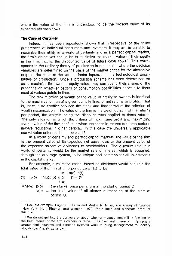
where the value of the firm is understood to be the present value of its expected net cash flows.

The Case of Certainty Indeed, it has been repeatedly shown that, irrespective of the utility

preferences of individual consumers and investors, if they are to be able to maximize their utility in a world of certainty and in a perfect capital market, the firm's objectives should be to maximize the market value of their equity in the firm, that is, the discounted value of future cash flows.2 This corre-sponds to the ordinary theory of production in economics where the decision variables are determined on the basis of the market prices for the alternative outputs, the costs of the various factor inputs, and the technological possi-bilities of production. Once a production scheme has been determined so as to maximize the owners' equity value, they can spend their shares of the proceeds on whatever pattern of consumption possibilities appeals to them most at various points in time.

The maximization of wealth or the value of equity to owners is identical to the maximization, as of a given point in time, of net returns or profits. That is, there is no conflict between the stock and flow forms of the criterion of wealth maximization. The value of the firm is the weighted sum of the returns per period, the weights being the discount rates applied to these returns. The only situation in which the criteria of maximizing profit and maximizing market value of the firm conflict is when increases in returns for some periods involve reductions in other periods. In this case the universally applicable market value criterion should be used.3

In a world of certainty and perfect capital markets, the value of the firm is the present value of its expected net cash flows or the present value of the expected stream of dividends to stockholders. The discount rate in a world of certainty would be the market rate of interest which is assumed, through the arbitrage system, to be unique and common for all investments in the capital market.

For example, a valuation model based on dividends would stipulate the total value of the firm at time period zero (to) to be

∞ n(o) d(t) (1) v(o) = n(o)p(o) = Σ (1+r) t

t = 1 Where: p(o) = the market price per share at the start of period O.

v(o) = the total value of all shares outstanding at the start of period O.

2 See, for example, Eugene F. Fama and Merton N. Miller, The Theory of Finance (New York: Holt, Rinehart and Winston, 1972) for a lucid and elaborate proof of this rule.

3 We do not get into the controversy about whether management will in fact act in the best interest of the firm's owners or rather in its own best interests. It is usually argued that incentive and sanction systems work to bring management to identify stockholders' goals as its own.

144

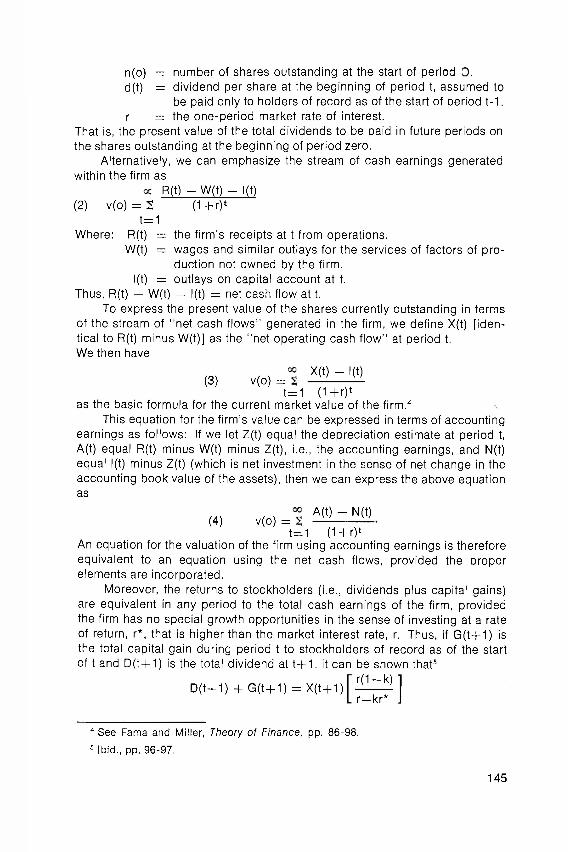
n(o) = number of shares outstanding at the start of period O. d(t) = dividend per share at the beginning of period t, assumed to

be paid only to holders of record as of the start of period t-1. r = the one-period market rate of interest.

That is, the present value of the total dividends to be paid in future periods on the shares outstanding at the beginning of period zero.

Alternatively, we can emphasize the stream of cash earnings generated within the firm as

∞ R(t) - W(t) - l(t) (2) v(o) = S (1+r) t

t = 1 Where: R(t) = the firm's receipts at t from operations.

W(t) = wages and similar outlays for the services of factors of pro-duction not owned by the firm.

I(t) = outlays on capital account at t. Thus, R(t) - W(t) - l(t) = net cash flow at t.

To express the present value of the shares currently outstanding in terms of the stream of "net cash flows" generated in the firm, we define X(t) [iden-tical to R(t) minus W(t)] as the "net operating cash flow" at period t. We then have

D(t+1) + G(t+1) = X(t+1) [r(1 — k) ]

r - k r *

4 See Fama and Miller, Theory of Finance, pp. 86-98. 5 Ibid., pp. 96-97.

145

(3) v(o)

∞ = Σ

t = 1 X(t) - l(t)

(1+r) t as the basic formula for the current market value of the firm.4

This equation for the firm's value can be expressed in terms of accounting earnings as follows: If we let Z(t) equal the depreciation estimate at period t, A(t) equal R(t) minus W(t) minus Z(t), i.e., the accounting earnings, and N(t) equal l(t) minus Z(t) (which is net investment in the sense of net change in the accounting book value of the assets), then we can express the above equation as

(4) v(o)

∞ = Σ

t— 1 A(t) - N(t)

( 1 + r ) t An equation for the valuation of the firm using accounting earnings is therefore equivalent to an equation using the net cash flows, provided the proper elements are incorporated.

Moreover, the returns to stockholders (i.e., dividends plus capital gains) are equivalent in any period to the total cash earnings of the firm, provided the firm has no special growth opportunities in the sense of investing at a rate of return, r*, that is higher than the market interest rate, r. Thus, if G(t+1) is the total capital gain during period t to stockholders of record as of the start of t and D(t+1) is the total dividend at t+1 , it can be shown that5

6 See Fama and Miller, Theory of Finance, p. 97. 7 For example, Fama and Miller, Theory of Finance, p. 84, in refuting the bird- in-the-

hand argument emphasize that " . . . the independence proposit ion does not require stockholders to be indifferent as between a present dividend and a future dividend or capital gains. It says, rather, that once management is committed to undertake and finance a given investment program, an increase in the dividends in any period will simply lead to a corresponding reduction in the ex-dividend value of the shares in the same period. . . ."

146

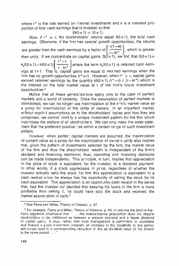
where r* is the rate earned on internal investments and k is a constant pro-portion of total cash earnings that is invested so that

Xk(t+1) = l ( t+1) . Now, if r* = r, the stockholders' returns equal X(t+1), the total cash

earnings. Otherwise, if the firm has special growth opportunities, the returns

are greater than the cash earnings by a factor of r ( 1 - k )

r - k r * , which is greater

than unity. If we concentrate on capital gains, G(t+1), we find that G(t+1) =

k rX(t+1) + kX(t+1) r * —r

r—kr* where the term k rX(t+1) is retained cash earn-

ings at t+1 . That is, capital gains are equal to retained earnings when the firm has no growth opportunities (r* = r). However, when r* > r, capital gains exceed retained earnings by the quantity kX(t+1) (r* — r) / (r—kr*) which is the interest on the total market value at t of the firm's future investment opportunities.6

Notice that all these generalizations apply only to the case of perfect markets and a world of certainty. Once the assumption of perfect markets is abandoned, we can no longer use maximization of the firm's market value as a proxy for maximization of the utility of owners. In an imperfect market, without explicit assumptions as to the stockholders' tastes and how they are comprised, we cannot identify a unique investment pattern for the firm which maximizes the welfare of all stockholders. We can only make the weak state-ment that the preferred position lies within a certain range of such investment pattern.

However, when perfect capital markets are assumed, the maximization of current value as a proxy for the maximization of owner's utility also implies that, given the pattern of investments selected by the firm, the market value of the firm and thus the shareholders' wealth is independent of the firm's dividend and financing decisions; thus, operating and financing decisions can be made independently. This principle, in turn, implies that appreciation in the price of stock is equivalent, for the investor, to a dividend payment. In other words, if a stock appreciates in price, regardless of whether the investor actually sells the stock, for him this appreciation is equivalent to a cash receipt since he always has the opportunity of selling the stock for its cash equivalent. This appreciation is an opportunity cash receipt in the sense that, had the investor not decided that keeping his funds in the firm is more profitable than selling it, he could have sold the stock and received the market appreciation in cash.7

Having thus shown that the value to a stockholder of his holding is identical to the present value of his expected stream of dividends or to the present value of the firm's cash earnings, it is now relevant to ask whether accounting should quantify this value. After all it could be argued that, if such identity exists, the value of the firm is already quantified through the market mechanism in the price of the stock. Thus, there would be no need to quantify it in the accounting report.

The Case of Uncertainty However, if the assumption of a world of certainty is relaxed, the market

value of the stock reflects not only the present value of expected dividends or cash flows to the firm but also the uncertainty associated with the flows. In other words, the uncertainty and the degree of risk associated with the occurrence of the expected cash flows are considered by transactors in the marketplace when they determine the market value of capital instruments through supply and demand.

In a world of uncertainty, the expectation of the firm's management with respect to both the magnitude of cash flows and their uncertainty may differ from that of transactors in the general marketplace. As a result, the market value of the securities will not necessarily be identical to the present value of cash flows as expected by the firm's management. But management ex-pectations regarding future cash flows and their uncertainty may represent useful information which enables market transactors to predict cash flows and their associated uncertainty. Transactors must make these predictions in order to facilitate their own decision-making.

Both the future cash flows and their uncertainty depend on the specific plans and actions that are implemented by, and first known to, the firm's management. Since such plans are designed to give the firm a competitive edge, they are bound to have significant informational content. Because the firm's management is the first to know its plans, timely forecasts by manage-ment with respect to future cash flows may prove to be a valuable input to the users of financial statements in their predictions of future cash flows. Management is in the best position to assess the effects of its specific plans on cash flows. The question is, are there market forces that would make these plans and the cash flows derived from them known to the market in the absence of a requirement for forecasts to be published by management? This question is discussed in detail in the paper entitled "The Need for Accounting Objectives in an Efficient Market," pages 36-52, where it was con-cluded that there is a need for management to communicate its forecast of cash flows.

Cash Flow Expectations. Generally, cash flows that a firm generates are influenced by two major factors:

1. Market and industry events that affect all firms, i.e., exogenous factors. 2. The particular performance of the firm in question, i.e., the specific plans

and decisions made by management. These firm-specific decisions are

147

responsible for whether the firm accumulates more or less value than the industry or the market. These are the endogenous factors.

It is of particular importance that management communicate the cash flows contingent on its plans.8 Since these plans are under management control, any deviation from them would reflect on management ability to predict and/or to perform. Exogenous factors, contrary to the endogenous, are pri-marily beyond the firm's control and may be predicted by relying on market expectations as a whole as reflected in market prices. However, the best source for predicting endogenous factors is probably the firm's management itself. As indicated, by obtaining management predictions of endogenous cash flows, users can assess management predictive ability and possibly performance. Also, information about management's particular plans and the actual results provides insights into risk-taking tendencies of management and therefore its future likelihood of engaging in risk-taking activities. How-ever, since cash flows are a joint result of both endogenous and exogenous factors, management can only communicate, its forecasts of the total cash flows resulting from both factors; but at the same time it could, and perhaps should, explicitly state its assumptions relative to the exogenous factors. In fact, management could provide forecasts of cash flows that are conditional on different assumptions regarding the exogenous factors. By doing this, users can evaluate these assumptions and make adjustments, if necessary, in the forecasts for their own decision-making purposes.

It is suggested that management communicate its forecasts of cash flows separate from its consideration of uncertainty associated with them. The pri-mary reason for the separation is that users' preferences and their assess-ments of the risk inherent in future events (both exogenous and endogenous) may differ from management's. If management's prediction of the magnitude of cash flows is disclosed separate from its judgment concerning risk and uncertainty, users will be able to combine the components to fit their own judgments and preferences toward risk. Users cannot do this if they are given only one value, that is, the magnitude of cash flows combined with the risk and uncertainty perceived by the firm's management.

Management is thus potentially a more useful source for predicting the endogenous factors under its control than for predicting exogenous factors. For example, with respect to exogenous factors, different information sources have different degrees of usefulness and competence in providing informa-tion about relevant events. Interest rate fluctuations, the money supply, and credit terms are factors, information on which is probably best obtained from the Federal Reserve; whereas, information on the availability of raw materials and future prices is probably best obtained through observing trends in the supplying industries. With respect to some events, the best source for pre-

8 Since the detailed plans do not have to be made available, but only the manage-ment's expectation of cash flows that are contingent on the plans, there should be no reluctance on management's part to communicate this information out of fear of leakage to competitors.

148

dieting the exogenous factors is probably the market itself. The research on efficient markets indicates that available information in a market9 (including information about exogenous factors relevant to the particular firm) is gener-ally impounded in market prices of securities or other capital assets. Market prices therefore best reflect the effects of relevant exogenous factors on the firm (although publicly available endogenous information would also be re-flected). For example, fluctuations in the price of a firm's output reflect antici-pated change in demand, which is a relevant exogenous factor affecting the firm. Similarly, fluctuations in the market prices of inputs would reflect ex-pectations with respect to changing conditions in the supplying industry and in the industries of competing inputs.

Reporting Both Discounted Cash Flows And Exit Values

In a frictionless market, prices are unique; that is, entry and exit values are identical. But they may differ in a market in which transaction costs exist. Since we also wish to provide measures of risk separately from expected magnitudes of cash flows, it seems reasonable to provide market prices at exit values of firm's assets rather than at entry values. Exit values of assets reflect not only the opportunity costs of holding assets within a firm10 but also the potential cash proceeds that are available to the firm in case of unfavor-able market conditions. Consequently, both management forecasts of ex-pected cash flows and the exit values of the firm's assets and liabilities should be communicated.11

Ronen and Sorter12 provide a detailed discussion of the advantages of such combined reporting and recommend the accounting reports to be com-municated. Ingredients of this system consist not only of expected cash flows and exit values but also actual transactions. The latter will enable users to assess the reliability of future forecasts by comparing management forecasts and actual events. Expected and unexpected results of operations are also distinguished to highlight the deviation of actual events from forecasted events. The quantification of unexpected events provides a record of man-

9 See, for example, Joshua Ronen, "The Need for Accounting Objectives in an Efficient Market," pp. 36-52, and Eugene F. Fama, "Eff icient Capital Markets: A Review of Theory and Empirical Work," Journal of Finance (May 1970), pp. 383-417.

10 The marginal cost of capital services per unit equals rpb + (pb—pe) where pb and pe are the prices per unit of capital at the beginning and end of the period respectively, and r is the one-period rate of return. The optimal investment of an asset is found at the point at which this cost is equated with the marginal cash flow that can be generated by the asset (see, for example, Fama and Miller, Theory of Finance, p. 117).

11 Exit values are also discounted cash flows. But these reflect the consensus ex-pectations of market transactors with respect to both the magnitude of cash flows and the risk associated with them, as discussed below.

12 Joshua Ronen and George H. Sorter, "Relevant Account ing," Journal of Business (April 1972), pp. 258-282.

149

agement's "errors" and would be useful in assessing—through the observa-tion of the magnitude of the errors over an extended period of time—the ability of management to forecast within a reasonable range of accuracy.

A summary of the combined Discounted Cash Flow (DCF)-Exit Value System is presented below in order to make this presentation as self-con-tained as possible.

The DCF-Exit Value System. Generally, discounted cash flow accounting refers to the quantification of the firm's value or "wealth" by discounting its expected net cash flows over a specified time period. The total value of a firm would thus be communicated in the annual report at the present value of cash flows as of the report date; this value may be separated into specific assets and liabilities reflecting for each asset and liability the present value of the expected contributions to the cash flows of the firm.13 While the indi-vidual values assigned to assets and liabilities—reflecting expected contri-butions to cash flows—would not necessarily add up to the total value of the firm, the separate communication may be useful for evaluating the manage-ment of the individual assets and liabilities.

By communicating both the total value and its decomposition into assets, a statement of resources is provided. The equities side of the balance sheet reflects particular configurations of the means with which the firm's manage-ment chose to obtain resources. To emphasize the importance of the asset side in the decision process that underlies a commitment of resources to enhance value to owners, it is useful to include both sides of the balance sheet under the statement of resources. Assets are employed in a particular manner so that they grow in value. The increment in value inures to the owners and creditors and is reflected in the equities side of the balance sheet. Viewing resources in this fashion provides a dynamic perspective within which the relation between resources and income can be interpreted. Thus, a statement of resources is not just a static reflection of wealth and the liabilities of the firm at an arbitrary point in time. Instead it is a procession of accumulated values at discrete points in time that reflects how resources change in value.

Annual income (assuming no dividends) is merely the difference in the value of the firm at the beginning and the end of the year. In this sense, the income statement articulates with the statement of resources. It converts the stock or value into a flow per period. Flow or income can also be separated into components; the particular segregation should be the one that helps users most in predicting cash flows and their uncertainty. For example, in-come can be separated into changes in the individual values of assets and liabilities.

There exist two quantifications of expected cash flows: the cash flow that is expected by the firm's management and the cash flow that is expected by all others. The latter is quantified through the market value of assets of the firm (which reflects the cash flows expected to be generated by the indi-vidual assets and the associated risks as perceived by market transactors).

13 This aspect will be discussed later.

150

The market value of the firm is reflected in the market price of its stock. The former, that is, discounted cash flows as expected by management, quantifies management's specific expectations of flows that jointly result from the ex-ogenous, uncontrollable events of the environment, and management's own plans and decisions, i.e., the endogenous events. One possible quantifica-tion of market prices of assets that reflects the cash flow as expected by the market is exit values. These values reflect the net proceeds that would be received if the assets were to be sold separately in the ordinary course of business. In a perfect, frictionless market, exit values and entry values are identical, and both uniquely determine a market price for an asset. In a market where there are transaction costs, however, these values would di-verge. Exit values are preferable because they also reflect the minimum opportunity costs of the asset, that is, their value if they are sold.14

In addition to the exit values of the separate assets as a quantification of cash flows as expected by the market, the contribution of these assets to the present value of cash flows as expected by management should be reported even though the total of these former values would not necessarily be identical to the present value of cash flows for the firm as a whole as expected by management. The difference between the latter and the sum of the values of the separable assets would reflect any assets for which there exists no present market, such as managerial know-how and the ability to combine the factors of production in a more efficient way than competitors. The present value of the firm's cash flow expectations would simply be the sum of the exit values of the separable assets plus the discounted value of the additional cash flows generated by special opportunities. Exit values reflect the ex-ogenous value of the assets, whereas the difference between the discounted cash flow value and the exit values reflects the incremental cash flows that management expects to result from the endogenous factors.

In order to present a general outline of the combined DCF-Exit value system it is usful to summarize its various elements separately.

The Market Risk-Determined (MRD) Value of the Firm. We discount the expected cash flows at the market average rate of return to obtain the total value of the firm which we call the market risk-determined value (MRD).15

By discounting the expected cash flows at the market rate of interest which reflects only general market risks, we provide a value for the firm which does not reflect the firm's specific risks. The reasons for doing this were

14 Although there may be within the firm alternative employments for the assets that generate larger benefits than those obtained when the assets are sold, these alternatives are both decision and time specific, and it is difficult to report them con-tinuously and on a systematic basis through the accounting system. Selling the assets, however, is an alternative that is always available, and quantif ication in this case is usually reliably ascertainable. See, for example, J. C. McKeown, "An Empirical Test of a Model Proposed by Chambers," Accounting Review (January 1971), pp. 12-29.

15 This value is ascertained by discounting expected cash flows at the average rate of return on all stocks listed on the New York Stock Exchange which would thus incorporate the average market risk.

151

explained above. The primary objective of reflecting value and risk sepa-rately is to allow different users to attach their own weights to the various determinants of value. Thus, by providing disaggregated information, users will be able to identify and evaluate the components of risk and value in line with their individual preferences.

Economic Income. The economic income of the firm is simply the change in its MRD value. It consists of two major elements: the time growth of the discounted cash flows and the revision of expectations concerning these cash flows. The time growth is an increment of the MRD value resulting from the passage of time. It is quantified by applying the market rate of return to the MRD value of the firm, and it indicates that all previously expected cash flows are now expected one period sooner. The second element is the revision of expectations which would result if the newly gained information will cause a change in either the magnitude of the expected cash flows or their time pattern.16

Exit Values. The individual assets and liabilities of the firm are quantified at their exit values. Exit value is the proceeds that could be obtained from selling an asset (in the case of an asset) or the payment needed to discharge an obligation (in the case of a liability or stock equity), net of transaction costs.17 The exit value of net assets is the difference between the exit values of assets and liabilities.

It is recognized that the assets of the firm have both a universal and a particular value. The exit value of an asset is its universal value, that is, what the asset can generate when not a part of bundles of unique assets that define the particular firm. The particular value of the asset is its marginal contri-bution in producing the firm's cash flows. The particular value of the firm's assets taken as a whole is the MRD value. A distinction is made between the exit values of two groups of assets: cash assets and noncash assets. Less uncertainty is associated with the realization of cash assets (cash, market-able securities, and accounts receivable). The consensus on the exit value of cash assets is more readily available than for other assets. Their conversion to cash is either guaranteed or required by law. This is generally not the case for other assets such as inventory, where conversion into cash depends upon events partially controlled by others. The degree of controllability affects the realization and thus the uncertainty associated with the different assets.

16 Alternative ways exist for quantifying expectations. For example, probability distributions of cash flows could be presented rather than point estimates. Also, cash expectations could be presented by time periods rather than aggregated through discounting them. However, point estimates rather than probability distributions and discounting to a present value are necessary if quantif ication by means of a single number is desired. At any rate, further investigation is needed to discriminate among the alternative quantifications and presentations.

17 Groups of assets could be quantified in the aggregate rather than individually. Theoretically the exit value of the assets would be measured and communicated with respect to those groups of assets for which the total sales value less transaction costs is maximized.

152

Therefore, the exit values of cash assets and other assets are separately reported.

Risk Indications. Comparison of the MRD value with the exit value of the firm's net assets can provide insights into some aspects of risk.18 The differ-ence between them is defined as the specific advantage of the firm. The difference between the firm's MRD value and the exit value of stockholders' equity is defined as the specific residual.

The specific advantage reflects that part of the expected flows that can-not be realized unless the firm continues its specific operations and continues to assume the risks associated with these operations. Exit values of the firm's net assets represent the cash flows that could be realized if the firm does not continue its specific operations; they are independent of uncertainties asso-ciated with the specific operations.

The specific residual reflects that portion of the expected flows that has not been captured by the market value of the firm's securities either (a) because the market assigned a risk factor that is higher than the general market risk to the firm's expectations, (b) because the market does not accept the magnitude of the future cash flows as reflected in the firm's expectations, or (c) through a combination of these two phenomena.

Both the specific advantage and the specific residual provide insights into aspects of risk and need not necessarily coincide. For example, the higher the specific advantage, the greater are the uncertainties associated with the realization of the firm's expectations, and the greater is the firm's exposure to an eventual decline in its value. Also, the expected variability of cash flows is likely to be higher for the firm which has a higher proportion of specific advantage to MRD value. Several factors contribute to the relation between the specific advantage and the specific residual and risk. These factors are fully discussed in Ronen and Sorter, "Relevant Accounting," cited in note 12, above.

The MRD value need not necessarily equal the firm's exit value (the market price of its stock equity). The difference between the two would reflect the difference in expectations between the managers and the market with respect to cash flows and their uncertainty. The firm's exit value (the market price of the stock equity), which is the market's expectation of flows that

15 Risk depends on the fol lowing major elements: (a) Probabilities associated with expected cash flows, (b) the covariance of the expected cash flows with the alternative cash flows available to information users (see, for example, Fama, "Eff icient Capital Markets," pp. 383-417), and (c) the degree of uncertainty associated with the realization of the expected flows. (While the degree of uncertainty may manifest itself in the variability of cash flows, there are advantages to considering these elements separately, in the absence of explicit knowledge about the extent to which such uncertainty affects the probability distributions.) Another element of risk associated with the above, that deserves to be separately identified, is (d) the extent to which the realization of these expected cash flows is within the firm's control. For instance, cash flows expected through the collection of accounts re-ceivable are generally more within the firm's control and less under the influence of others than the cash flows expected through the sale of most products. The more controllable the realization of flows, the less risk may be associated with these flows.

153

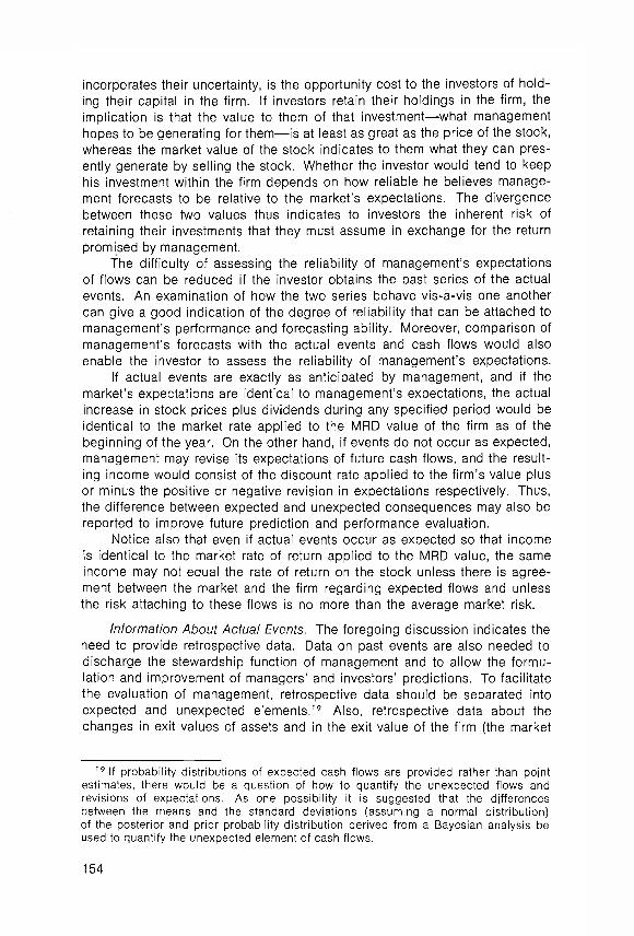
incorporates their uncertainty, is the opportunity cost to the investors of hold-ing their capital in the firm. If investors retain their holdings in the firm, the implication is that the value to them of that investment—what management hopes to be generating for them—is at least as great as the price of the stock, whereas the market value of the stock indicates to them what they can pres-ently generate by selling the stock. Whether the investor would tend to keep his investment within the firm depends on how reliable he believes manage-ment forecasts to be relative to the market's expectations. The divergence between these two values thus indicates to investors the inherent risk of retaining their investments that they must assume in exchange for the return promised by management.

The difficulty of assessing the reliability of management's expectations of flows can be reduced if the investor obtains the past series of the actual events. An examination of how the two series behave vis-a-vis one another can give a good indication of the degree of reliability that can be attached to management's performance and forecasting ability. Moreover, comparison of management's forecasts with the actual events and cash flows would also enable the investor to assess the reliability of management's expectations.

If actual events are exactly as anticipated by management, and if the market's expectations are identical to management's expectations, the actual increase in stock prices plus dividends during any specified period would be identical to the market rate applied to the MRD value of the firm as of the beginning of the year. On the other hand, if events do not occur as expected, management may revise its expectations of future cash flows, and the result-ing income would consist of the discount rate applied to the firm's value plus or minus the positive or negative revision in expectations respectively. Thus, the difference between expected and unexpected consequences may also be reported to improve future prediction and performance evaluation.

Notice also that even if actual events occur as expected so that income is identical to the market rate of return applied to the MRD value, the same income may not equal the rate of return on the stock unless there is agree-ment between the market and the firm regarding expected flows and unless the risk attaching to these flows is no more than the average market risk.

Information About Actual Events. The foregoing discussion indicates the need to provide retrospective data. Data on past events are also needed to discharge the stewardship function of management and to allow the formu-lation and improvement of managers' and investors' predictions. To facilitate the evaluation of management, retrospective data should be separated into expected and unexpected elements.19 Also, retrospective data about the changes in exit values of assets and in the exit value of the firm (the market

19 If probability distributions of expected cash flows are provided rather than point estimates, there would be a question of how to quantify the unexpected flows and revisions of expectations. As one possibility it is suggested that the differences between the means and the standard deviations (assuming a normal distribution) of the posterior and prior probability distribution derived from a Bayesian analysis be used to quantify the unexpected element of cash flows.

154

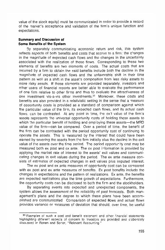
value of the stock equity) must be communicated in order to provide a record of the market's acceptance and validation of the firm's unique function and expectations.

Summary and Discussion of Some Benefits of the System

By separately communicating economic return and risk, this system reflects aspects of both benefits and costs that accrue to a firm: the changes in the magnitude of expected cash flows and the changes in the uncertainty associated with the realization of these flows. Corresponding to these two elements of benefits are two elements of costs. The actual costs that are incurred by a firm to obtain the said benefits include both the decline in the magnitude of expected cash flows and the unfavorable shift in their time pattern as well as a shift in the asset's composition from less risky assets to more risky assets. If these elements are provided separately, investors and other users of financial reports are better able to evaluate the performance of one firm relative to other firms and thus to evaluate the attractiveness of one investment vis-a-vis other investments.20 Moreover, these costs and benefits are also provided in a relativistic setting in the sense that a measure of opportunity costs is provided as a standard of comparison against which the particular value of the firm, its expected cash flows, and its actual cash flows, can be contrasted. At any point in time, the exit value of the firm's assets represents the universal opportunity costs of holding these assets to which the particular benefit of holding and employing these assets—the MRD value of the firm—can be compared. Over a period of time, the benefit of the firm can be contrasted with the period opportunity cost of continuing to operate the assets. This is measured by the interest that could have been earned by severing the assets from the firm initially plus the decline in the exit value of the assets over the time period. The period opportunity cost may be measured both ex post and ex ante. The ex post information is provided by applying the market rate of interest to the assets' exit values and communi-cating changes in exit values during the period. The ex ante measure con-sists of estimates of expected changes in exit values plus imputed interest.

The ex post and ex ante measures of opportunity cost can be compared with ex post and ex ante measures of benefits. Ex post benefits include the changes in expectations and the pattern of realizations. Ex ante, the benefits are expected realizations plus the time growth of expectations. Furthermore, the opportunity costs can be disclosed to both the firm and the stockholders.

By separating events into expected and unexpected components, the system allows the assessment of the reliability of past forecasts. Both man-agement's plans and the degree to which these plans have been accom-plished are communicated. Comparison of expected flows and actual flows provides variance or measures of deviation that should, over time, be useful

2 0 Examples of such a cost and benefit statement and other financial statements highlighting different aspects of concern to investors are provided and elaborately discussed in Ronen and Sorter, "Relevant Accounting "

155

in assessing the success of the firm and of its management. When such devi-ations are reported for all firms as a result of wide adoption of the system, comparative measures of deviation will thus be provided making it possible to evaluate the performance and the capability of managements of different firms. Also, the general adoption of the system will allow investors to con-trast and measure the covariability of the given firm's flows and expectations with the flows and expectations of other firms.21

Appendix

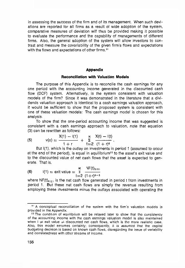
Reconciliation with Valuation Models

The purpose of this Appendix is to reconcile the cash earnings for any one period with the accounting income generated in the discounted cash flow (DCF) system. Alternatively, is the system consistent with valuation models of the firm? Since it was demonstrated in the literature that a divi-dends valuation approach is identical to a cash earnings valuation approach, it would be sufficient to show that the proposed system is consistent with one of these valuation models: The cash earnings model is chosen for this analysis,

To show that the one-period accounting income that was suggested is consistent with a cash earnings approach to valuation, note that equation (3) can be rewritten as follows:

X(1) — I(1) ∞ X(t) —I(t) (5) V(o) = Σ 2 .

1 + r t = 2 (1 + r)t But 1(1), which is the outlay on investments in period 1 (assumed to occur

at the end of the period), is equal in equilibrium22 to the asset's exit value and to the discounted value of net cash flows that the asset is expected to gen-erate. That is,

∞ X(t)-I(t) (6) 1(1) = exit value = Σ

t = 2 (1 + r ) t - 1

where NF(t) I ( 1 ) is the net cash flow generated in period t from investments in period 1. But these net cash flows are simply the revenue resulting from employing these investments minus the outlays associated with operating the

21 A conceptual reconciliation of the system with the firm's valuation models is provided in the Appendix.

22 The condition of equilibrium will be relaxed later to show that the consistency of the accounting income with the cash earnings valuation model is also maintained when I ≠ e x i t v a l u e ≠ d i s c o u n t e d net cash flows, which is the more realistic case. Also, this model assumes certainty; consequently, it is assumed that the capital budgeting decision is based on known cash flows, disregarding the issue of variability and correlatedness with other streams of income.

156

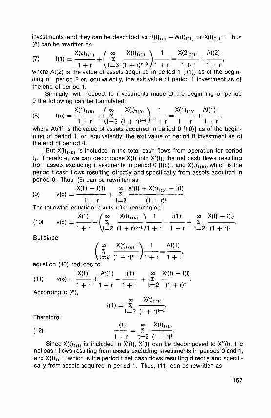
investments, and they can be described as R(t) I (1 )— W(t}1(1) or X( t ) I ( 1 ) . Thus (6) can be rewritten as

(7) 1(1) = X(2)I(1)

1 + r +

∞ Σ

t = 3

X(t)I(1)

(1 + r ) t -2

1

1 + r

X(2)I(1) At(2)

1 4- r +

1 + r where At(2) is the value of assets acquired in period 1 [1(1)] as of the begin-ning of period 2 or, equivalently, the exit value of period 1 investment as of the end of period 1.

Similarly, with respect to investments made at the beginning of period 0 the following can be formulated:

(8) l(o) = X(1)I(1)

1 + r +

∞

Σ

t = 2

X(t)I(1)

(1 + r ) t - 1 ;

1

1 + r

X(1)I(1)

1 + r +

At(1)

1 + r where At(1) is the value of assets acquired in period 0 [I<0)] as of the begin-ning of period 1, or, equivalently, the exit value of period 0 investment as of the end of period 0.

But X(t) I ( 0 ) is included in the total cash flows from operation for period t1. Therefore, we can decompose X(t) into X'(t), the net cash flows resulting from assets excluding investments in period 0 [l(o)], and X(t) I ( 0 ) , which is the period t cash flows resulting directly and specifically from assets acquired in period 0. Thus, (5) can be rewritten as

(9) v(o) = X(1) — 1(1)

1 + r +

∞

Σ

t = 2

X'(t) + X(t)I(1) - l(t)

(1 + r)t The following equation results after rearranging:

(10) v(o) = X(1)

1 + r +

∞

Σ

t = 2

X(t) I ( 0 )

(1 + r ) t - 1

1

1 + r

1(1)

1 + r +

∞ Σ t = 2 X(t) - l(t)

(1 + r)t But since

∞ Σ t = 2 X(t)I(1)

(1 + r ) t - 1

1

1 + r

At(1)

1 + r equation (10) reduces to

(11) v(o) = X(1)

1 + r +

At(1)

1 + r

1(1)

1 + r +

∞ Σ t = 2 X'(t) - l(t)

(1 + r)t According to (6),

Therefore:

I(1) =

∞ Σ

t = 2

X(t)I(1)

(1 + r ) t - 1

1(1)

1 + r

∞

Σ

t = 2

X(t)I(1)

(1 + r ) t

(12)

Since X(t) I ( t ) is included in X'(t), X'(t) can be decomposed to X"(t), the net cash flows resulting from assets excluding investments in periods 0 and 1, and X(t) I ( 1 ) , which is the period t net cash flows resulting directly and specifi-cally from assets acquired in period 1. Thus, (11) can be rewritten as

157

23 It can be similarly shown that when investments are made during the period, the discounted cash value of these investments at the time of purchase should be similarly subtracted to obtain the period's income.

158

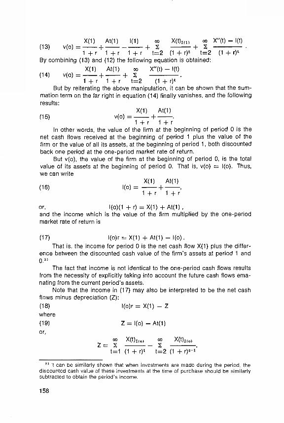
(13) v(o) = X(1) At(1) 1(1)

1 + r 1 + r 1 + r

∞ Σ

t = 2

X(t)I(0)

(1 + r)t

∞ Σ

t = 2

X"(t) - l(t)

(1 + r)t By combining (13) and (12) the following equation is obtained:

(14) v(o) = X(1) At(1)

1 + r 1 + r

∞ Σ

t = 2

X"(t) - l(t)

(1 + r) t But by reiterating the above manipulation, it can be shown that the sum-

mation term on the far right in equation (14) finally vanishes, and the following results:

(15) v(o) = X(1) At(1)

1 + r 1 + r In other words, the value of the firm at the beginning of period 0 is the

net cash flows received at the beginning of period 1 plus the value of the firm or the value of all its assets, at the beginning of period 1, both discounted back one period at the one-period market rate of return.

But v(o), the value of the firm at the beginning of period 0, is the total value of its assets at the beginning of period 0. That is, v(o) = l(o). Thus, we can write

(16) l(o) = X(1) At(1)

1 + r 1 + r

or, l(o)(1 + r ) = X ( 1 ) + A t ( 1 ) , and the income which is the value of the firm multiplied by the one-period market rate of return is

(17) l(o)r = X ( 1 ) + A t ( 1 ) - l ( o ) . That is, the income for period 0 is the net cash flow X(1) plus the differ-

ence between the discounted cash value of the firm's assets at period 1 and 0.2 3

The fact that income is not identical to the one-period cash flows results from the necessity of explicitly taking into account the future cash flows ema-nating from the current period's assets.

Note that the income in (17) may also be interpreted to be the net cash flows minus depreciation (Z): (18) l(o)r = X(1) — Z where (19) Z = l(o) — At(1) or,

Z = ∞

Σ

t = 1

X(t) I ( 0 )

(1 + r)t

∞

Σ

t = 2

X(t)I(0)

(1 + r ) t - 1

159

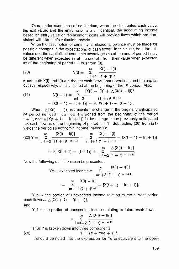
Thus, under conditions of equilibrium, when the discounted cash value, the exit value, and the entry value are all identical, the accounting income based on entry value or replacement costs will provide flows which are con-sistent with the firm's valuation models.

When the assumption of certainty is relaxed, allowance must be made for possible changes in the expectations of cash flows. In this case, both the exit values and the capitalized economic advantages as of the end of period t may be different when expected as of the end of t from their value when expected as of the beginning of period t. Thus from (3),

(20) V(t) = ∞

Σ

i = t + 1

X(i) - l(i)

(1 + r )i-t where both X(i) and l(i) are the net cash flows from operations and the capital outlays respectively, as envisioned at the beginning of the t th period. Also,

(21) V ( t + 1 ) = ∞

Σ

i = t + 2

[ X ( i ) - I ( i ) ] + A [ X ( i ) - l ( i ) ]

(1 + r)1_( t+1)

+ [X(t + 1) - l(t + 1)] + [X(t + 1) - l ( t + 1)].

Where [X(i) — l(i)] represents the change in the originally anticipated i t h period net cash flow now envisioned from the beginning of the period t + 1, and [X(t + 1) — l(t + 1)] is the change in the previously anticipated net cash flow as of the beginning of period t + 1. Subtracting (20) from (21) yields the period t's economic income (hence Y):

(22) Y = ∞ Σ

i = t + 2

[X(i) - l(i)]

(1 + r ) 1 + 1 )

∞ Σ

i = t + 1 (1 + r )i-t

X(i) - l(i) [X(t + 1 ) - l ( t + 1)]

+ [X ( t+ 1) - l ( t + 1)] +

∞ Σ

i = t + 2 (1 + r)i-(t+1)

,[X(i) - l(i)]

Now the following definitions can be presented:

Ye = expected income ∞ Σ

i = t + 2 (1 + r ) i - ( t + 1 )

[X(i) - l(i)]

∞ Σ

i = t + 1 (1 + r ) i - t

X(i) - l(i) + [X(t + 1) - l(t + 1)],

Yue = the portion of unexpected income relating to the current period cash flows = [X(t + 1) - l(t + 1)], and

Yuf = the portion of unexpected income relating to future cash flows ∞ Σ

i = t + 2 (1 + r ) i _ ( t + 1 )

[X(i) - l(i)]

Thus Y is broken down into three components (23) Y = Ye + Yue + Yuf.

It should be noted that the expression for Ye is equivalent to the oper-

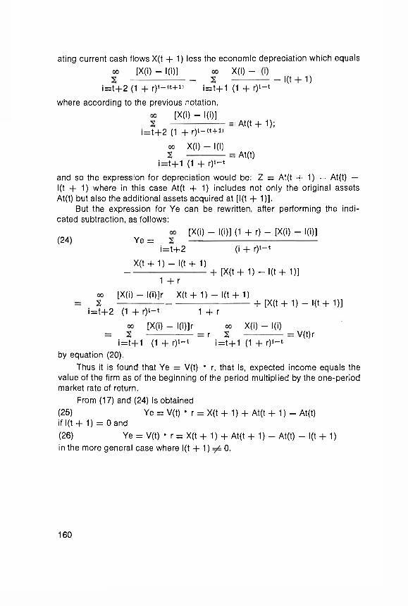
ating current cash flows X(t + 1) less the economic depreciation which equals ∞ Σ

i = t + 2 (1 + r ) 1 _ ( t + 1 )

[X(i) - l(i)] ∞ Σ

i = t + 1 (1 + r ) i - t

X(i) - I(i) l ( t + 1 )

where according to the previous notation, ∞ Σ

i = t + 2 (1 + r ) i - ( t + 1 )

[X(i) - l(i)] : At(t + 1);

∞ Σ

i = t + 1 (1 + r ) i - t

X(i) - l(i) At(t)

and so the expression for depreciation would be: Z = At(t + 1) — At(t) — l(t + 1) where in this case At(t + 1) includes not only the original assets At(t) but also the additional assets acquired at [l(t + 1)].

But the expression for Ye can be rewritten, after performing the indi-cated subtraction, as follows:

(24) Ye = ∞ Σ

i = t + 2

[X(i) - l(i)] (1 + r) - [X(i) - l(i)]

(i + r ) i - t

X ( t + 1) - l ( t + 1)

1 + r [X(t + 1) — l(t + 1)]

∞ Σ

i = t + 2 (1 + r ) i - t

[X(i) — l(i)lr X ( t + 1 ) - l(t + 1 )

1 + r [X(t + 1) — l(t + 1)]

∞ Σ

i = t + 1

[X(i) - l(i)]r

(1 + r ) i - t r

∞ Σ

i = t + 1 (1 + r ) i - t

X(i) - l(i) V(t)r

by equation (20). Thus it is found that Ye = V(t) • r, that is, expected income equals the

value of the firm as of the beginning of the period multiplied by the one-period market rate of return.

From (17) and (24) is obtained Ye = V(t) • r = X(t + 1) + At(t + 1) - At(t) (25)

if l(t + 1) = 0 and (26) Ye = V(t) • r = X(t + 1) + At(t + 1) - At(t) - l(t + 1) in the more general case where l(t + 1 ) ≠ 0 .

160