DIRECTION GÉNÉRALE DES ÉTUDES ET DES RELATIONS INTERNATIONALES

Disaster Risk and Preference Shifts in a New Keynesian Model

Marlène Isoré 1 & Urszula Szczerbowicz 2

Working Paper 614

December 2016

ABSTRACT

In RBC models, “disaster risk shocks” reproduce countercyclical risk premia but generate an increase in consumption along the recession and asset price fall, through their effects on agents’ preferences (Gourio, 2012). This paper offers a solution to this puzzle by developing a New Keynesian model with such a small but time-varying probability of “disaster”. We show that price stickiness, combined with an elasticity of intertemporal substitution smaller than unity, restores procyclical consumption and wages, while preserving countercyclical risk premia, in response to disaster risk shocks. The mechanism then provides a rationale for discount factor first- and second-moment (“uncertainty”) shocks.

Keywords: disaster risk, rare events, uncertainty, Epstein-Zin-Weil preferences, asset pricing, DSGE models, New Keynesian models, business cycles, risk premium. JEL classification: D81, D90, E20, E31, E32, E44, G12, Q54.

1 University of Helsinki and Bank of Finland 2 Banque de France

Working Papers reflect the opinions of the authors and do not necessarily express the views of the Banque de France or the Bank of Finland. This document is available on the Banque de France Website.

Les Documents de travail reflètent les idées personnelles de leurs auteurs et n'expriment pas nécessairement la position de la Banque de France ou de la Banque de Finlande. Ce document est disponible sur le site internet de la Banque de France.

NON-TECHNICAL SUMMARY3

During the 2007-2009 financial crisis, risk premia increased significantly in advanced economies and central banks implemented various unconventional monetary policies in order to reduce them. However, generating realistic risk premia along with expected macroeconomic variations in response to shocks is particularly challenging in standard economic models. We show that incorporating a time-varying “disaster risk” in a New Keynesian model allows to reproduce countercyclical risk premia together with the expected co-movement of macroeconomic variables, in particular consumption, investment, and wages, along the recession. In that respect, we improve some of the macroeconomic predictions from real business cycle (RBC) analysis of disaster risk and generalize the mechanism into a policy-friendly framework.

A central feature of our model relies on the likelihood that rare disasters hit the economy. Rare disasters are large adverse events associated with a low probability, such as great recessions, wars, terrorist attacks or natural catastrophes. They can lead to important declines in production, consumption, capital, or productivity. Rietz (1988) and Barro (2006) showed that accounting for these events can explain the high level of risk premia observed in the data, incompatible with previous standard asset pricing models (equity premium puzzle). Furthermore, Gabaix (2011), Gourio (2012), and Wachter (2013) developed dynamic models which allow the probability of disasters to be time-varying. In particular, Gourio (2012) introduced a small time-varying probability of disaster, defined as an event that destroys a large share of the existing capital stock and productivity, into RBC model. An interesting implication is that an increase in the probability of disaster, without occurrence of the disaster itself, suffices to trigger a recession and replicate key asset pricing regularities.

However, this literature faces two limitations. First, an increase in disaster risk generates a recession and a drop in stock prices, but it also increases consumption which seems counterfactual. Second, the model generates output and investment drops only under the assumption that the agents have a very large adaptability to substitute consumption across periods in response to shocks. In other terms, the elasticity of intertemporal substitution (EIS) parameter needs to be set to a value strictly greater than unity. Should the EIS be lower than unity, the results are completely reversed. In particular, a rise in the probability of disaster would then generate a boom in output and investment. Empirical evidence on the EIS is mixed, yet values below unity are realistic and conventionally adopted in macroeconomic calibrations. Therefore, such a contrasting response of output from changes in disaster risk at the unity threshold seems particularly puzzling.

In this paper, we introduce a small time-varying probability of disaster à la Gourio (2012) into an otherwise standard New Keynesian model. To the best of our knowledge, we are the first to do so.

3 We thank George-Marios Angeletos, Guido Ascari, Pierpaolo Benigno, Nick Bloom, Ambrogio Cesa-Bianchi, Fabrice Collard, Luca Dedola, Martin Ellison, Francesco Furlanetto, Xavier Gabaix, François Gourio, Oren Levintal, Vivien Lewis, Julien Matheron, Antonio Mele, Afrasiab Mirza, Stefan Niemann, Salvatore Nisticò, Juan Carlos Parra-Alvarez, Julien Penasse, Johannes Pfeifer, Antti Ripatti, Kjetil Storesletten, Fabien Tripier, Philippe Weil, Raf Wouters, and Francesco Zanetti, as well as participants at numerous seminars and conferences, for fruitful discussions. M. Isoré is grateful to the Yrjö Jahnsson Foundation for financial support on this project.

Banque de France Working Paper 614 ii

The main result of our paper consists in demonstrating that price stickiness, combined with an EIS below unity, is able to restore procyclicality of the main macroeconomic quantities. In particular, we show that agents become more “patient” in response to disaster risk shocks. Their propensity to save increases while their consumption declines, such that deflation follows. Yet, higher savings do not immediately translate into higher investment, such that output also drops. As a result, an increase in disaster risk leads to simultaneous falls in investment, consumption, prices, and output as capital becomes riskier. As for asset prices, we observe a ‘flight-to-quality’ effect that is visible through the drop in the risk-free rate when the disaster risk shock hits, as well as the increase in the risk premium. Hence, while improving Gourio (2012)’s predictions for the macroeconomic variables, we preserve the strength of his mechanism for accounting for the countercyclicality of the risk premia.

The intuition works as follows. Let us consider for instance the case of an EIS below unity. An increase in disaster risk decreases agents’ propensity to consume such that savings go up. Because of price stickiness, firms cannot deflate their good prices as much as they would like to face reduced consumption and thus demand fewer factors of production, capital and labor. Therefore, despite precautionary motives, all macroeconomic quantities go down with output. Since the return on capital is riskier after the increased probability of disaster, the risk premium is countercyclical. Overall, we thus show that introducing a time-varying disaster risk à la Gourio (2012) into a full-fleshed New Keynesian model is critical, not just to enrich the macroeconomic setting and spectrum of potential policy analysis, but because it literally conditions most of the qualitative effects associated with a change in disaster risk, for a given value of the EIS.

Following Gourio (2012)’s solution method, the effects of disaster risk on preferences are embedded into agents’ discount factor. However, this discount factor goes up in our model, as agents’ patience increases when the EIS is below unity, whereas it was going down in Gourio (2012)’s. Combined with price stickiness, the responses of aggregate macroeconomic and financial variables to a disaster risk shock in turn resemble the responses to a preference shock (Christiano et al. (2011)) and a second-moment “uncertainty” shock (Basu and Bundick (2015)). In that sense, we show how Gourio (2012)’s mechanism of disaster risk can be conciliated with these other shocks from the New Keynesian literature, recently found to drive the economy into the zero lower bound and secular stagnation. We thus provide a milestone model which could be used for further investigation of monetary policy responses to changes in the probability of disaster events.

Banque de France Working Paper 614 iii

RÉSUMÉ : Risque de désastre et changement de préférences dans le modèle néo-keynésien

Dans les modèles de cycles réels, un choc de « risque de désastre » permet bien de reproduire la contra-cyclicité des primes de risque mais génère une hausse de la consommation, simultanément à une récession et une chute de prix des actifs, via ses effets sur les préférences des agents (Gourio, 2012). Cet article répond à ce problème théorique en développant un modèle néo-keynésien comprenant une telle probabilité de « désastre » faible mais variable dans le temps. Nous montrons que la rigidité des prix, associée à une élasticité de substitution inter-temporelle inférieure à un, rétablit la pro-cyclicité de la consommation et des salaires tout en préservant la contra-cyclicité des primes de risque en réponse aux chocs de risque de désastre. Le mécanisme fournit alors une source possible de chocs sur les premier et second moments du facteur d’escompte, respectivement dits chocs de préférences et d’« incertitude ». Mots-clés : risque de désastre, événements rares, incertitude, préférences Epstein-Zin-Weil, évaluation des actifs financiers, modèles DSGE, modèles néo-keynésiens, cycles économiques, prime de risque.

Banque de France Working Paper 614 iv

1 Introduction

Recent years have seen renewed interest in the economic impact of ‘rareevents’. In particular, Gabaix (2011, 2012) and Gourio (2012) have intro-duced a small but time-varying probability of ‘disaster’, defined as an eventthat destroys a large share of the existing capital stock and productivity, intoreal business cycle (RBC) models. The main result is that an increase in theprobability of disaster, without occurrence of the disaster itself, suffices totrigger a recession and replicate key asset pricing regularities.

However, this literature faces two limitations. First, an increase in disas-ter risk generates a recession and a drop in stock prices, but it also increasesconsumption. Yet, recent estimations from option price tails document thatdisaster risk tends to increase in periods of financial distress and recessions(Siriwardane (2015)), while such episodes are themselves correlated withcontemporaneous declines in consumption (see Albuquerque et al. (2015)for e.g). Second, the model predictions for output and asset pricing rely onthe elasticity of intertemporal substitution (EIS) being set to a value strictlygreater than unity, but are completely reversed otherwise.1 In particular,a rise in the probability of disaster generates a boom in output should theEIS be lower than unity, everthing else equal. Empirical evidence on the EISis mixed, yet values below unity are realistic and conventionally adopted inmacroeconomic calibrations, whether the models feature Epstein-Zin-Weilpreferences or not.2 Therefore, such a contrasting response of output fromchanges in disaster risk at the unity threshold seems particularly puzzling.

In order to address these caveats, we introduce a small time-varyingprobability of disaster à la Gourio (2012) into an otherwise standard NewKeynesian model. To the best of our knowledge, we are the first to do so.3

The contribution is threefold. First, we nest Gourio (2012)’s mechanism of1Barro (2009) shows that the aggregate stock market declines with the probability of

disaster only when the EIS is greater than one with Epstein-Zin-Weil preferences. Gourio(2012)’s recessionary effects of the disaster risk rely on the same condition.

2See Section 4 for further related discussion.3Two previous attempts of disaster risk into a New Keynesian model include Isoré and

Szczerbowicz (2013), considering the capital depreciation effect of disaster risk only, andBrede (2013) where the ‘disaster state’ is permanent and deterministic, i.e the economyentering a disaster state stays there forever. In contrast, we keep the essence of Gourio(2012) in considering disaster risk as a time-varying source of uncertainty here. Finally,despite a title close to ours, Andreasen (2012) studies skewed shock distributions in aDSGE model, which quite differ from the formalization of disaster risk we adopt here.

1

disaster risk into a New Keynesian setup and shed light on the critical roleof the EIS in driving the sign of macroeconomic responses to a disaster riskshock. In particular, when prices are flexible, we obtain an output boomwith an EIS below unity, and a recession together with an increase in con-sumption, wages, and prices with an EIS above unity. Second, we show thatprice stickiness provides a simple solution to this puzzle. Indeed, it allows toconciliate the recessionary effects of disaster risk with an EIS below unity,as well as to restore the expected comovements of other macroeconomic andasset pricing variables. In that respect, we improve some of macroeconomicpredictions from Gourio (2012)’s mechanism of disaster risk and generalizethe analysis to a policy-friendly framework. Third, we conciliate this mecha-nism with the New Keynesian literature on discount factor shocks. Changesin disaster risk produce a mix of first- and second-moment effects on agents’(endogenized) discount factor. Yet, in Gourio (2012)’s RBC model, theyboth contribute to agents’ impatience, such that lower savings then causethe recession. In contrast, increased patience drives the recession via lowerconsumption levels, in our setup. This result is very much in line with theNew Keynesian literatures on (i) exogenous ‘preference shocks’ defined asshocks to the level of the discount factor (Smets and Wouters, 2003, Chris-tiano et al., 2011, for e.g), and (ii) ‘uncertainty shocks’ defined as shocksto the volatility of the discount factor (Basu and Bundick, 2015). There-fore, it supports the interpretation of disaster risk as a potential source ofuncertainty in future economic conditions.

The intuition works as follows. The occurrence of a disaster would destroyparts of the capital stock and productivity.4 The probability of such an eventgoing up suffices to create a mix of depreciation and uncertainty effects on thefuture return on capital. Agents’ response depends on the relative valuationof substitution and income effects, which is determined by the value of theEIS. Indeed, as known since Leland (1968) and Sandmo (1970), an increase ininterest rate risk increases (decreases) agents’ propensity to consume (save),and thus reduces savings (consumption), if and only if the EIS is larger than1.5 In a RBC setup, the response of savings drives investment, and therefore

4Disasters can be alternatively modeled as large declines in consumption (Barro (2006),Wachter (2013)). Yet, in models including a production sector, they are most often rep-resented by a drop in capital and/or productivity (Barro (2009), Gabaix (2011), Gourio(2012)). We follow Gourio (2012) so as to nest his results as a particular case of our model.

5Weil (1990) shows that a large EIS implies that the elasticity of savings to a ‘certainty-

2

output, despite an opposite response in consumption. Hence, with an EISabove unity, agents invest less when disaster risk goes up, and a recessionensues. Under some assumptions, Gourio (2012) captures this mechanism byendogenizing the discount factor as a negative function of disaster risk whenthe EIS is above unity. Should the EIS be below unity, the exact oppositeholds, i.e the economy is booming as disaster risk goes up.

The additional presence of sticky prices does not alter the effect of the EISon agents’ willingness to consume/save. However, the aggregate dynamicsbecome more impacted by the demand side (consumption) than the supplyside (savings) of the economy. Take for instance the case of an EIS belowunity such that consumption goes down and savings go up in response to anincrease in disaster risk. Because of price stickiness, firms cannot deflate asmuch as they would like to face reduced consumption and thus demand lessfactors of production, capital and labor. Therefore, despite precautionarymotives, all quantities co-move and output is driven down. Since the returnon capital is riskier, the risk premium remains countercyclical.6 Overall, wethus show that introducing a time-varying disaster risk à la Gourio (2012)into a full-fleshed New Keynesian model is critical, not just to enrich themacroeconomic setting and spectrum of potential policy analysis, but be-cause it literally conditions most of the qualitative effects associated with achange in disaster risk, for a given value of the EIS.

The remainder is as follows. The rest of the introduction briefly reviewsthe literature and our related contribution. Section (2) presents the model.Section (3) describes the solution method and emphasizes the analytical roleof the EIS in driving the qualitative results from disaster risk shocks. Section(4) discusses the calibration and steady-state values. In particular, Tallar-ini (2000)’s “observational equivalence” holds in the presence of disaster riskwhen the EIS is equal to unity, but not for any other value above or belowthat threshold. Section (5) simulates a positive shock on the probability ofdisaster. We find that the combination of sticky prices and an EIS belowunity is able to generate a recession, jointly with a drop in consumption,

equivalent’ interest rate is positive, i.e savings decrease in the aggregate interest rate risk.On the contrary, a small EIS implies that savings go up with interest rate risk.

6Basu and Bundick (2015) show that “uncertainty” shocks (as exogenous second-moment discount factor shocks) also generate very different qualitative economic responsesdepending on price stickiness/flexibility. In particular, they argue that only stickiness gen-erates a positive co-movement of consumption and investment, as observed in the data.

3

investment, hours and wages, a deflation, and an increase in the risk pre-mium. We also show that all other combinations of EIS below/above unityand price flexibility/stickiness generate either a boom or a negative macroe-conomic comovements along the recession. Section (6) concludes.

Literature review.Our paper is related to two main strands of literature. First, the literature

on ‘rare events’, sometimes called economic ‘disasters’, which emerged as aresponse to the equity premium puzzle (Mehra and Prescott, 1985). Indeed,Rietz (1988), Barro (2006), and Barro and Ursúa (2008) introduced a smallconstant probability of an economic disaster into endowment economies andshowed it able to replicate the size of the risk premium.7 Yet, the volatilityand countercyclicality of the risk premium, as well as the stock price-dividendratio, return predictability and the bond risk premia, were still not accountedfor.8 Therefore, Gabaix (2008) first considered the probability of disaster tobe time-varying into an endowment economy, before Gabaix (2011, 2012)and Gourio (2012, 2013) further introduced it into RBC models.9

Although successful in reproducing the size, volatility, and countercycli-cality of risk premia, these RBC models still leave room for improvementin the responses of the macroeconomic variables to disaster risk shocks. In-deed, macroeconomic quantities are unresponsive to changes in disaster riskin Gabaix (2012), in line with Tallarini (2000)’s “observational equivalence”where only asset prices are affected by aggregate risks. Gourio (2012) showsthat this result holds only for an EIS strictly equal to unity, but not for anyother value as disaster risk shocks then impact agents’ preferences and sub-sequently macroeconomic variables. However, some responses seem counter-factual, such as consumption in particular. Empirical analyses on the effectsof disaster risk variations are quite new but tend to suggest that consumptiondecreases and becomes more volatile with disaster risk (Marfè and Penasse,2016, for e.g).10 More evidence tend to associate estimated time series of dis-

7Numerous alternative solutions have been provided to this puzzle but we choose notto enumerate them here for concision as this is not the main focus of our paper.

8In Barro and Ursúa (2008), the price-dividend ratio and the risk-free rate are constant.9An Epstein-Zin-Weil (EZW) utility function is a necessary ingredient, that we also

adopt here, yet not sufficient to address the equity premium puzzle alone. Especially, Weil(1989) must set the risk aversion coefficient to 45 and the EIS to 0.1 in order to obtain areasonable match with the data. Yet, it matters for dissociating the degree of risk aversionfrom the value of the EIS. Here as in Weil (1990), risk aversion will impact the size of themacroeconomic responses to aggregate risks while the EIS will determine their sign.

10We are not aware of any opposite evidence as of to date.

4

aster risk to periods of recessions and stock price falls (Siriwardane, 2015),while such episodes are commonly associated with lower consumption.11 Wethus build on Gourio (2012)’s approach here but try to restore the expectedsign of some quantities, consumption, wages, and output prices, in particular.

Second, our paper is related to literatures on preference and uncertaintyshocks. Indeed, following Gourio (2012)’s approach, disaster risk creates amix of first- and second-moment effects on agents’ discount factor in themodel. Preference shocks have also been praised as an early solution tocapture asset pricing phenomena, such as the equity premium, the bondterm premium, and the weak correlation between stock returns and funda-mentals, that supply-driven shocks alone could not (Campbell and Ammer(1993), Cochrane (2011)). The intuition is that they affect agents’ demandfor riskfree assets, and thus generate a good fit for riskfree rate variations,independently of cash flows (Campbell (1986), Schorfheide et al. (2014)).

However, these models, as well as Gourio (2012), find that a negativepreference shock, i.e a decrease in agents’ discount factor, is associated withrecessions and stock price falls. This sharply contrasts with the New Key-nesian literature where similar effects stem from a positive preference shock.Indeed, a higher degree of patience drive agents’ demand for risky assetsdown and favor ‘fly-to-quality’ effects.12 Thereby, positive preference shocksare very successful in driving the economy to the zero lower bound (ZLB)on the nominal policy rate in New Keynesian setups (Eggertsson and Wood-ford (2003), Christiano et al. (2011), Erceg and Linde (2012), Eggertssonet al. (2014)).13 Empirical variance decompositions support positive pref-erence shocks as a major determinant of the nominal interest rate (Smetsand Wouters (2003) and Ireland (2004)). Our model suggests that Gourio(2012)’s mechanism of disaster risk, which endogenizes preference shifts, canbe seen as a rationale for positive – rather than negative – preference shockswhen the combination of an EIS below unity and sticky prices is at play. We

11Siriwardane (2015) estimates time series of a“risk-neutral” probability of disaster frominformation contained in the cross-section of option and equity returns. He finds it strongly(negatively) correlated to periods of recessions and lower stock prices .

12Smets and Wouters (2003)’s DSGE model of the euro area include such a preferenceshock for instance. Smets and Wouters (2007), estimated on US data, consider a slightlydifferent shock which directly affects agents’ preference for riskfree assets (Fisher, 2015).

13As the discount factor increases, agents’ propensity to consume decreases, puttingdownward pressure on real factor prices, real marginal cost, and inflation. In turn, theinterest rate diminishes to reduce deflationary pressures.

5

thus restore its compatibility with that branch of the literature.Finally, second-moment discount factor shocks, sometimes referred to as

‘uncertainty’ shocks, matter. Bloom (2009) first stressed the sharp reces-sionary effects of uncertainty shocks, formalized as productivity volatilityshocks. More recently, Basu and Bundick (2015) found a simultaneous de-cline in output, consumption, investment, and hours worked, in response tosecond-moment discount factor shocks when price stickiness is at play intoa New Keynesian setup.14 15 Our responses resemble theirs but stem froman endogenous mechanism of preference shifts induced by disaster risk. Inthat sense, changes in disaster risk can be seen as a rationale for uncertaintyshocks. This idea is supported empirically by Baker and Bloom (2013), forinstance, who use rare events, such as natural disasters, terrorist attacks,political coups d’état and revolutions to instrument for changes in the leveland volatility of stock-market returns. They argue that some shocks, likenatural disasters, lead primarily to a change in stock-market levels (first-moment shocks), while other shocks like coups d’état lead mainly to changesin stock-market volatility (second-moment shocks).

2 Model

2.1 Households

Households derive utility from consumption and leisure, accumulate capitaland bonds, own monopolistic competition firms to which they rent capitaland labor force, earn profits, and pay lump-sum taxes.

Households’ Epstein-Zin-Weil preferences are given by

Vt =

[[Ct (1− Lt)$]1−ψ + β0

(EtV

1−γt+1

) 1−ψ1−γ] 1

1−ψ

(1)

14In a similar spirit, Leduc and Liu (2016) find that nominal rigidities amplify the effectof uncertainty shocks on the unemployment rate through declines in aggregate demand.

15Bloom (2009) and Basu and Bundick (2015) consider the VIX and alternative measuresof uncertainty to support their predictions with a VAR analysis. We are unfortunatelynot able to reproduce it with estimated measures of disaster risk such as Marfè andPenasse (2015) or Siriwardane (2015) since those series are very new and not available yet.However, in a recent discussion of our paper (Banque de France, October 2016), JulienPenasse showed that consumption indeed declines in response to one standard deviationdisaster risk shock using their estimated series of disaster risk (Marfè and Penasse, 2016).This discussion is available on request.

6

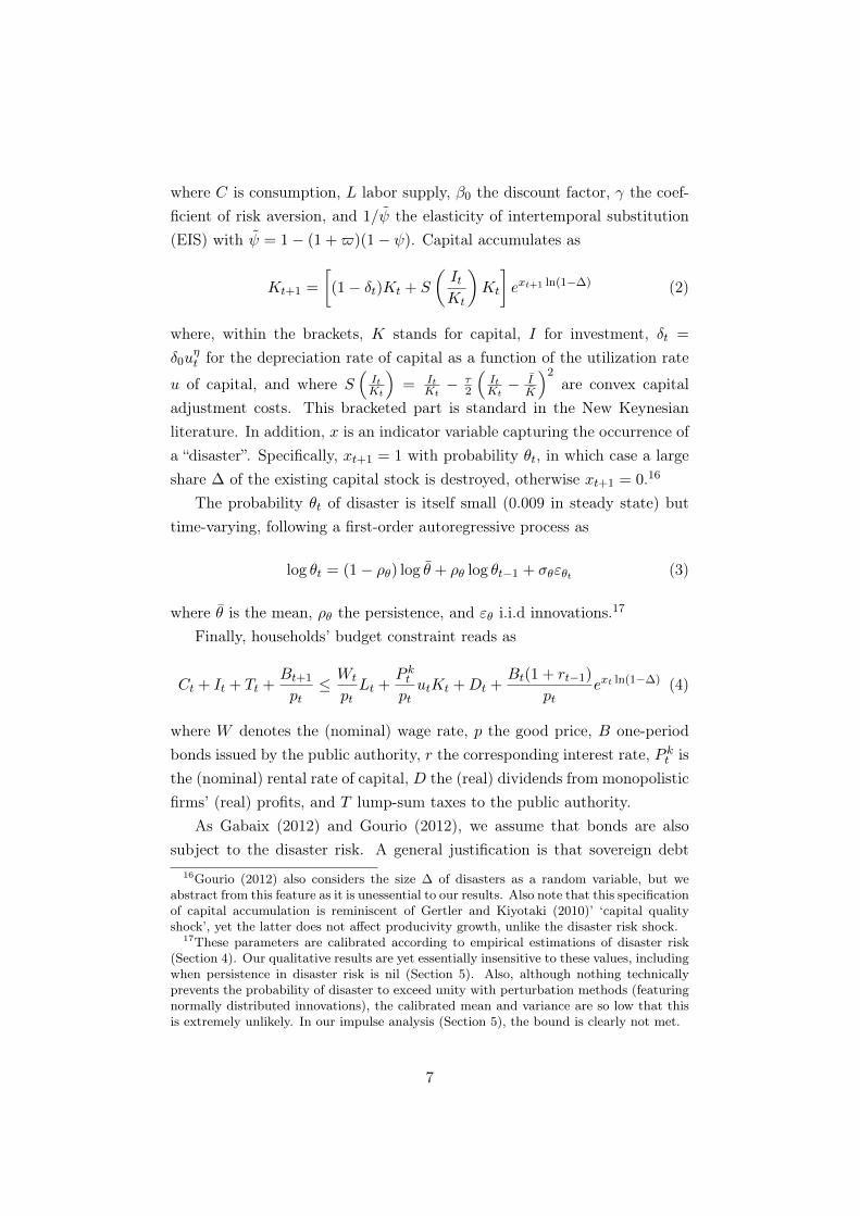
where C is consumption, L labor supply, β0 the discount factor, γ the coef-ficient of risk aversion, and 1/ψ the elasticity of intertemporal substitution(EIS) with ψ = 1− (1 +$)(1− ψ). Capital accumulates as

Kt+1 =

[(1− δt)Kt + S

(ItKt

)Kt

]ext+1 ln(1−∆) (2)

where, within the brackets, K stands for capital, I for investment, δt =

δ0uηt for the depreciation rate of capital as a function of the utilization rate

u of capital, and where S(ItKt

)= It

Kt− τ

2

(ItKt− I

K

)2are convex capital

adjustment costs. This bracketed part is standard in the New Keynesianliterature. In addition, x is an indicator variable capturing the occurrence ofa “disaster”. Specifically, xt+1 = 1 with probability θt, in which case a largeshare ∆ of the existing capital stock is destroyed, otherwise xt+1 = 0.16

The probability θt of disaster is itself small (0.009 in steady state) buttime-varying, following a first-order autoregressive process as

log θt = (1− ρθ) log θ + ρθ log θt−1 + σθεθt (3)

where θ is the mean, ρθ the persistence, and εθ i.i.d innovations.17

Finally, households’ budget constraint reads as

Ct + It + Tt +Bt+1

pt≤ Wt

ptLt +

P ktptutKt +Dt +

Bt(1 + rt−1)

ptext ln(1−∆) (4)

where W denotes the (nominal) wage rate, p the good price, B one-periodbonds issued by the public authority, r the corresponding interest rate, P kt isthe (nominal) rental rate of capital, D the (real) dividends from monopolisticfirms’ (real) profits, and T lump-sum taxes to the public authority.

As Gabaix (2012) and Gourio (2012), we assume that bonds are alsosubject to the disaster risk. A general justification is that sovereign debt

16Gourio (2012) also considers the size ∆ of disasters as a random variable, but weabstract from this feature as it is unessential to our results. Also note that this specificationof capital accumulation is reminiscent of Gertler and Kiyotaki (2010)’ ‘capital qualityshock’, yet the latter does not affect producivity growth, unlike the disaster risk shock.

17These parameters are calibrated according to empirical estimations of disaster risk(Section 4). Our qualitative results are yet essentially insensitive to these values, includingwhen persistence in disaster risk is nil (Section 5). Also, although nothing technicallyprevents the probability of disaster to exceed unity with perturbation methods (featuringnormally distributed innovations), the calibrated mean and variance are so low that thisis extremely unlikely. In our impulse analysis (Section 5), the bound is clearly not met.

7

can indeed be risky during tail events in the sense that it becomes subjectto partial default, as we have observed for Greece in the last financial crisis,Argentina in the early 2000s, and UK in the Great Depression, as for a fewexamples. Conditional on no disaster, bonds are however riskfree, unlikecapital. A more specific reason for the presence of risky bonds is a technicaltrick making the problem particularly easy to solve. Indeed, when the eventdestruction size ∆ is the same for both assets and productivity, then thedetrended system will not be directly impacted by the large disaster event(x) itself but only by the small probability of disaster (θ), which is ourvariable of interest, as explained more extensively in Section 4.18

Overall, households maximize their utility (1) subject to their capitalaccumulation (2) and budget (4) constraints, given the time-varying disasterrisk (3). Optimality conditions to this problem, given in Appendix, stillcontain the presence of the disaster event (x) at this stage. However, onlythe disaster probability (θ) will remain in the detrended equilibrium system,following Gourio (2012)’s solution method described further in Section 4.

2.2 Asset pricing

From the Epstein-Zin-Weil preferences defined above (1), the (real) stochas-tic discount factor can be calculated as

Qt,t+1 ≡∂Vt/∂Ct+1

∂Vt/∂Ct= β0

(Ct+1

Ct

)−ψ (1− Lt+1

1− Lt

)$(1−ψ) V −χt+1

(EtV1−χt+1 )

−χ1−χ

(5)

Then, asset pricing orthogonality conditions give the riskfree rate, Rf , asEt (Qt,t+1) = 1/Rft+1 known at time t, and the (real) rate of return on capital,

Rk,realt+1 , such that Et(Qt,t+1R

k,realt+1

)where the time-t expectation operator

accounts, together with other possible shocks, for a disaster realization int + 1. Note that the riskfree rate defined here is not the yield on the one-period bonds which are again risky, but rather a “natural” (gross) interest

18This feature is not essential to our results but makes the solution tractable. One canrelax it and use projection methods to solve for the model instead, but with qualitativelysimilar results as Gourio (2012) shows. Alternatively, one could as well take a stand onwhether the economy is currently in a disaster (x = 1) regime or not (x = 0) and generate(regime-contingent) impulse response functions to changes in disaster risk.

8

rate. Thus, the risk premium on capital holdings can now be defined as

Et(Risk premiumt+1) ≡ Et

(Rk,realt+1

Rft+1

)

which will be nil with a first-order approximation, constant with secondorder, and time-varying with third and higher orders.

2.3 Firms

The structure of production considered here is quite standard as for a NewKeynesian model. However, it plays crucial role for our results: unlike Gourio(2012)’s centralized economy flexible-price model, the decentralized economyfeaturing monopolistic competition and sticky prices allows to obtain reces-sionary effects from a disaster risk shock when the EIS is smaller than unity.The nominal price friction makes the reponse of output affected mostly bythe demand side (consumption) rather than the supply side (savings) of theeconomy. Thus, the drop in consumption associated with a rise in disasterrisk when the EIS is below unity will generate here recession and deflation.

Firms are operating in two sectors, final good production and intermedi-ate good production. The former market is competitive, while the latter ismonopolistic. They are briefly described below, see Appendix for details.

2.3.1 Final good production

The final good is an aggregate of intermediate goods j as given by

Yt =

(∫ 1

0Y

ν−1ν

j,t dj

) νν−1

where ν is the elasticity of substitution among intermediate goods. Profitmaximization gives a demand curve which is decreasing in the price of inter-mediate good j relative to the aggregate price index (pj,t/pt) as

Yj,t =

(pj,tpt

)−νYt

2.3.2 Intermediate sector

Intermediate sector firms use households’ capital and labor to produce goodsj, according to a Cobb-Douglas function with labor-augmenting productivity.

9

In each period, they optimize the quantities of factors they want to use,taking their prices as given, subject to the production function and theaggregate demand function at a given output price. Thet also set theirprice optimally at frequency determined by a constant Calvo probability.19

The intra-temporal problem (cost minimization problem) is thus

minLj,t,Kj,t

WtLj,t + P kt Kj,t

s.t. Kαj,t(ztLj,t)

1−α ≥(pj,tpt

)−νYt

where W stands for the (non-detrended) nominal wage rate, P k the capitalrental rate, and K ≡ uK the effective capital (with u the utilization rate ofcapital). The first-order conditions, expressed in detrended terms, are

(Lj,t :) wt = mcnomj,t (1− α)

(kj,tLj,t

)α

(Kj,t :) P kt = mcnomj,t α

(kj,tLj,t

)α−1

in which the Lagrange multiplier denoted mcnomj,t can be interpreted as the(nominal) marginal cost associated with an additional unit of capital orlabor. Rearranging further gives an optimal capital to labor ratio which isthe same for all intermediate firms in equilibrium.

Let’s now consider the inter-temporal problem of a firm that gets to up-date its price in period t and wants to maximize the present-discounted valueof future profits. Given the (real) profit flows that read as pj,t

ptYj,t −mc∗tYj,t

and the demand function Yj,t =(pj,tpt

)−νYt, the maximization problem is

maxpj,t

Et

∞∑s=0

(ζ)sQt+s

((pj,tpt+s

)1−νYt+s −mc∗t+s

(pj,tpt+s

)−νYt+s

)19It can be that firms adjust their price more frequently when disaster risk goes up.

In Isoré and Szczerbowicz (2013), we considered both time- and state-dependent price-adjustment settings. In the latter case, the probability of not adjusting one firm’s price canbe thought of as a decreasing function of disaster risk. Yet, the results are not significantlydifferent, such that we chose not to include this additional channel of disaster risk here.

10

where discounting includes both households’ stochastic discount factor, Qt,t+s,and the probability ζs that a price chosen at time t is still in effect at times. After some simplification, the first-order condition is

p∗j,t =ν

ν − 1Et

∑∞s=0 (ζ)sQt+sp

νt+sYt+smc

∗t+s∑∞

s=0 (ζ)sQt+spν−1t+s Yt+s

which depends on aggregate variables only, so that p∗t = p∗j,t. Increases inthis optimal price from one period to another will give us the reset inflationrate while increases in the current price level pt defines the current inflationrate. (see Appendix for more details.)

2.4 Public authority

Bonds clears with public debt issued by a public authority which raises taxesfrom the households. The public authority also sets up the nominal interestrate on bonds following a Taylor type rule as

rt = ρrrt−1 + (1− ρr) [Φπ(πt − π) + ΦY (yt − y∗) + r∗] (6)

2.5 Equilibrium

The equilibrium consists of the optimality conditions and constraints ofhouseholds, firms, and the public authority. They are reported in Section(A.1) of the Appendix.

3 Solution method

We here follow Gourio (2012) in detrending the equilibrium system by theproductivity level zt so as to eliminate the disaster event xt+1 itself, whilekeeping the disaster risk θt, in that system. This will not only bring someinsightful analytical results on the impact of the EIS, but it will also allowus to use standard perturbation methods on the detrended system in orderto simulate the impact of a (small) shock to the (small) probability of dis-aster θt. In the absence of any large event x itself, perturbation methodsbecome accurate to account for the response of macroeconomic quantities toa disaster risk shock already from a first order approximation, and for the

11

responses of the time-varying risk premia from the third order.20

This detrending method requires one additional assumption which is toassume that productivity is affected by disaster events, if any, in the sameproportion as the assets (physical capital and bonds).21 Specifically,

zt+1

zt= eµ+εz,t+1+xt+1 ln(1−∆) (7)

where µ is a technological trend and εz,t+1 are i.i.d normally distributedinnovations with zero mean.

The rest of this Section describes the detrending of some key equationsand stresses the intuition. The detrending of the full equilibrium system isrelegated to the Appendix.

As emphasized in Gourio (2012), the law of motion for capital is straight-forward. Indeed, using (7), (2) can be rewritten as

kt+1 =(1− δt)kt + S

(itkt

)kt

eµ+εz,t+1(8)

with δt = δ0uηt and with S

(itkt

)= it

kt− τ

2

(itkt− i

k

)2, where a lower case letter

denote a productivity-detrended variable (for e.g, kt = Kt/zt). Note thatindeed, the disaster indicator xt+1 has now vanished from (8) as opposed toits non-detrended counterpart (2).

Another important effect of that detrending can be seen from the Epstein-

Zin-Weil utility function. Indeed, denoting vt ≡(Vt/zt

)1−ψ, (1) becomes

vt = [ct(1− Lt)$]1−ψ + β(θ)e(1−ψ)µ

[Ete

(1−γ)εz,t+1v1−γ1−ψt+1

] 1−ψ1−γ

(9)

where

β(θ) = β0

[1− θt + θte

(1−γ) ln(1−∆)] 1−ψ

1−γ (10)

20Fernández-Villaverde and Levintal (2016) analyze the accuracy of perturbation andprojections methods in models with disasters. However, the shock they consider is adisaster size shock, for which they find that perturbation methods are not accurate belowthe fifth order, which is not surprising as the size is potentially large. We are not subjectto this criticism as long as we consider small deviations in a (small) disaster probability.

21Labor productivity may indeed decrease during financial crises (e.g Hughes and Sale-heen, 2012), as well as during wars or natural disasters as people may find themselves notnecessarily matched with jobs requiring their specific skills. Total factor productivity mayalso decrease as firms facing severe financing constraints may reduce their R&D expendi-tures (Millard and Nicolae, 2014). Gabaix (2012) and Gourio (2012)’s RBC models withdisaster risk both assume that the destruction share is the same than for the assets.

12

is a time-varying pseudo-‘discount factor’ as a function of the time-varyingdisaster risk. The appealing feature of this method is that the whole dy-namic effect of potential disasters is now captured by the presence of thistime-varying probability in agents’ discount factor. As discussed in Gourio(2012), a change in θt creates a mix of first- and second-moment effects onβ(θ) which reinforce one another in affecting macroeconomic quantities andasset prices.22 In that respect, this change in θt is expected to resemble botha ‘preference shock’ (in level) à la Smets and Wouters (2003) or Christianoet al. (2011), for examples, and a second-moment preference (‘uncertainty’)shock à la Basu and Bundick (2015). Before turning to the general equilib-rium effect of disaster risk shocks, let us have a further look at the crucialrole of the EIS on the sign of β(θ). Indeed, recall that we denoted the EISas 1/ψ with ψ = 1− (1 +$)(1− ψ), such that (10) can be rewritten as

β(θ) = β0

[1− θt

(1− e(1−γ) ln(1−∆)

)] 1−1/EIS(1−γ)(1+$) (11)

This expression makes it clear that the unity threshold of the EIS determinesthe sign of the effect of the probability of disaster (θ) on the discount factor,i.e on agents’ propensity to save or consume. Indeed, when EIS < 1, β(θ)

increases in θ, such that the households become more patient and save morewith disaster risk. On the contrary, when EIS > 1, β(θ) decreases in θ andimpatient agents tend to consume more in response to changes in disasterrisk. Note that this role of the EIS in determining the sign of β(θ) holds re-gardless of the degree of risk aversion of the agents, including risk neutrality,i.e for all γ ≥ 0, and regardless of price flexilibility or stickiness. Finally, forEIS = 1, β(θ) = β0 such that disaster risk will not impact macroeconomicquantities at all. This case is the so-called ‘Tallarini (2000)’s equivalence’,stating that macroeconomic quantities are determined irrespectively of thelevel of aggregate risk or risk aversion whenever EIS = 1.

In the general equilibrium, agents’ choice for saving or consuming inresponse to disaster risk shocks of course affects output. But the sign of thisoutput response differs whether prices are flexible or sticky. Indeed, whenprices are flexible, a higher propensity to save translates in higher investmentand thus higher output. Hence, the flexible-price case either predicts thatdisaster risk decreases output (while increasing consumption) with EIS > 1

22See the last paragraph on page 13 of Gourio (2012) for more about this.

13

(Gourio, 2012) or increases output with EIS < 1. On the contrary, a stickyenvironment makes firms unable to adjust their price to their optimal levelimmediately, affecting their demand of factors of production (capital andlabor) so as to maximize their profits (or minimize their loss). Specifically,when disaster risk increases agents’ propensity to save (when EIS < 1),consumption drops but firms cannot deflate prices as much as they would like.As a result, they demand less capital such that investment also falls despitehigher savings. The model is then able to predict the contemporaneous dropin all key macroeconomic variables in response to a disaster risk shock.

4 Calibration and steady-state analysis

4.1 Effect of the EIS on the balanced growth path

Using chain rules, the stochastic discount factor (20) can be rewritten as23

Qt,t+1 =ztzt+1

(ct+1

ct

)−ψ (1− Lt+1

1− Lt

)$(1−ψ)

β(θt)e(1−ψ)µ e(1−γ)εz,t+1v−χt+1[

Ete(1−γ)εz,t+1v1−χt+1

] −χ1−χ

which, along the balanced growth path, becomes

Q(x′) = β0e−ψµ−γx

′ ln(1−∆)(Ee(1−γ)x′ ln(1−∆)

)ψ−γ1−γ

where v′(k′) cancel out from the previous expression as they are independentfrom x′.24 Therefore, the orthogonality condition E(Q(x′)Rk(x′)) = 1 givesthe return on capital (along the balanced growth path) as

E(Rk(x′)) =E(ex

′ ln(1−∆))

β0e−ψµ(Ee(1−γ)x′ ln(1−∆)

) 1−ψ1−γ

and the constant riskfree rate from Rf = 1/E(Q(x′)) as23Note that this expression is still a function of the future disaster state, xt+1, as part

of the productivity growth term (zt/zt+1). We momentaneously use it to derive the assetpricing equations, but later combine it with the Euler equation on bonds such that only theprobability θ of disaster remains in our final equilibrium set (calculations in Appendix).

24Indeed, capital accumulation for the next period, k′, is independent from the occur-rence x′ of a disaster in its detrended version (8). Thus, so is v′(k′), as in Gourio (2012).Moreover, the arrival of x′ only depends on the current probability θ.

14

Rf =

(Ee(1−γ)x′ ln(1−∆)

)ψ−γ1−γ

β0e−ψµE(e−γx′ ln(1−∆)

)Note that the riskfree rate decreases in the disaster risk (along the balancedgrowth path), and the smaller the EIS, the larger the drop.25 This resultsis well known in the literature and often justifies the need for a use of anEIS larger than unity in order to limit the fall in the riskfree rate (Tsai andWatcher (2015).26 However, in our general equilibrium setup, price stickinessmakes the drop in the riskfree rate relatively lower when the EIS is belowunity rather than above.

Finally, the balanced growth path risk premium is given by

E(Rk(x′))

Rf=E(ex

′ ln(1−∆))E(e−γx′ ln(1−∆))

E(e(1−γ)x′ ln(1−∆)

)which, as expected, depends positively on the disaster risk, and the larger therisk aversion, the larger the effect. If agents were risk neutral, i.e when γ = 0,the risk premium is unaffected by changes in the probability of disaster. Notethat the EIS does not directly impact the value of the risk premium alongthe balanced growth path, in line with Gourio (2012), although its dynamicresponse to the disaster risk shock will eventually differ under alternativevalues of the EIS as a general equilibrium effect (See Section 5).27

4.2 Calibration

Table 1 summarizes our baseline calibration values. We also proceed tovarious sensitivity analyses presented in Section 5.3.

The first part of Table 1 is related to the calibration of disaster risk. Wefollow empirical estimates of the literature on historical data. Evidence is

25See the Appendix for calculation details.26An increase in disaster risk directly reduces the price of equities as it lowers expected

cash flows. But meanwhile, it causes an increase in precautionary savings which diminishesthe risk-free rate, and in turn tends to increase the price of equities by increasing demandrelatively to the supply of equities. Whether this latter effect offsets the former depends onthe value of EIS. Indeed, the smaller the EIS, the larger the precautionary savings and thedrop in the risk free rate. For example, Berkman et al. (2011) show that the probabilityof disasters, defined as political crises, is negatively correlated with stock prices. Evidenceof this kind encouraged the asset pricing literature to adopt an EIS larger than one.

27Gourio (2012) finds the same expression for the risk premium along the balancedgrowth path (Proposition 5). However, general equilibrium effects will differ here.

15

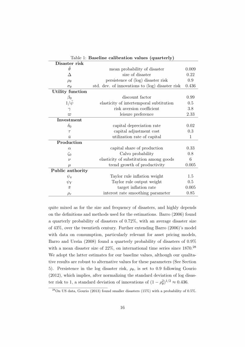
Table 1: Baseline calibration values (quarterly)Disaster risk

θ mean probability of disaster 0.009∆ size of disaster 0.22ρθ persistence of (log) disaster risk 0.9σθ std. dev. of innovations to (log) disaster risk 0.436

Utility functionβ0 discount factor 0.99

1/ψ elasticity of intertemporal subtitution 0.5γ risk aversion coefficient 3.8$ leisure preference 2.33

Investmentδ0 capital depreciation rate 0.02τ capital adjustment cost 0.3u utilization rate of capital 1

Productionα capital share of production 0.33ζ0 Calvo probability 0.8ν elasticity of substitution among goods 6µ trend growth of productivity 0.005

Public authorityψπ Taylor rule inflation weight 1.5ψY Taylor rule output weight 0.5π target inflation rate 0.005ρr interest rate smoothing parameter 0.85

quite mixed as for the size and frequency of disasters, and highly dependson the definitions and methods used for the estimations. Barro (2006) founda quarterly probability of disasters of 0.72%, with an average disaster sizeof 43%, over the twentieth century. Further extending Barro (2006)’s modelwith data on consumption, particularly relevant for asset pricing models,Barro and Ursúa (2008) found a quarterly probability of disasters of 0.9%with a mean disaster size of 22%, on international time series since 1870.28

We adopt the latter estimates for our baseline values, although our qualita-tive results are robust to alternative values for these parameters (See Section5). Persistence in the log disaster risk, ρθ, is set to 0.9 following Gourio(2012), which implies, after normalizing the standard deviation of log disas-ter risk to 1, a standard deviation of innovations of (1− ρ2

θ)1/2 ≈ 0.436.

28On US data, Gourio (2013) found smaller disasters (15%) with a probability of 0.5%.

16

The second part of Table 1 refers to the EZW utility function. Theinstantantaneous utility specification is borrowed from Gourio (2012) andwe thus adopt the same valuation of leisure ($ = 2.33). We also keep hisdegree of risk aversion coefficient (γ = 3.8), as it seems aligned with recentestimates in presence of disaster risk. Indeed, Barro and Jin (2011) found amean close to 3, with a 95% confidence interval for values from 2 to 4. Yet,we show in the sensitivity analysis, that the degree of risk aversion affectsonly the size but not the sign of the responses, confirming early theoreticalresults from Leland (1968), Sandmo (1970), and Weil (1990), for instance.

The only parameter in the second block of Table 1 which is crucial for ourresults and departs from Gourio (2012) is the value of the EIS. The empiricalevidence is quite mixed. Hall (1988)’s seminar paper found this parameterto be close to zero, and a subsequent literature has provided further supportfor values smaller than one (see e.g Campbell and Mankiw (1989), Lud-vigson (1999), Yogo (2004)).29 Yet, at least two types of concerns aboutthese estimates have been raised. First, agents’ heterogeneity matters: theEIS tends to be larger for richer households (Blundell et al. (1994), At-tanasio and Browning (1995)) and stockholders (Mankiw and Zeldes (1991),Vissing-Jorgensen (2002)), but much smaller for liquidity-constrained house-holds (Bayoumi (1993)). Second, the presence of uncertainty is an importantconcern for the estimates, although this is still under debate (Bansal andYaron (2004) Bansal et al. (2012), Beeler and Campbell (2012)).30 Turningto the theory, most of the macroeconomic RBC and DSGE models take avalue smaller than one. In particular, this holds whether preferences are ofGreenwood-Hercowitz-Huffman (GHH) type, potentially augmented with ex-ternal habits (for e.g Smets and Wouters (2003, 2007)), or Epstein-Zin-Weilwhere the EIS parameter does not need to be the inverse of the risk aversioncoefficient (for e.g Rudebusch and Swanson (2012), Caldara et al. (2012)).Yet, a notable exception are macro-finance models aiming at matching asset

29Havránek et al. (2015) have collected 2,735 estimates of EIS reported in 169 studiesto explore estimation differences across countries and methodologies from a meta analysis.They find a mean estimate around 0.5, and typically lying between 0 and 1. They suggestthat the type of utility function does not affect much the results.

30Bansal and Yaron (2004) argue that ignoring time-varying consumption volatility leadsto a downward bias in the macro estimates. Using an instrumental variable approach,Beeler and Campbell (2012) recognize the existence of the downward bias but do not findit large enough to question the low estimated values. Bansal et al. (2012) further criticizethe high sensitivity of their results to the samples, assets, and instruments they used.

17

pricing moments, where the EIS value is generally set above unity in orderto replicate the level, volatility, and cyclicality of financial returns and theequity premium. In that respect, models of disaster risk (Barro and Ursúa(2008), Gourio (2012), Nakamura et al. (2013)) generally set the EIS aboveunity (generally, at 2).31 Our approach here is not to impose any particularvalue of the EIS ex ante, but rather to select the one that gives the plau-sible responses to a disaster risk shock. In particular, we keep 0.5 as it isthe inverse from Gourio (2012)’s value of 2, and indeed find exactly opposedresponses of the macroeconomic variables. Yet, any value of the EIS up tounity would generate results qualitatively similar to our baseline responses,while any value above unity would reproduce Gourio (2012)’s. In that sense,we are able to make Gourio (2012)’s mechanism of disaster risk compatiblewith more standard macroeconomic calibrations.

The rest of Table 1 mostly follows the New Keynesian literature. Twovalues are still especially worth commenting here. First, we set the quarterlyCalvo probability of firms not changing their price the common value ofζ = 0.8. This may seem strong in the presence of aggregate risk, yet ourqualitative results are unchanged under a large span of lower degrees of pricestickiness (0.3-0.8), even though their size of course is. With low valuesof stickiness (<0.3), the responses become qualitatively similar to the pureflexible-price case (ζ = 0). Here as for the EIS, we do not need to take a standon the degree of price stickiness/flexibility in the presence of disaster risk exante, but rather aim at experimenting several combination of EIS and pricestickiness values before selecting the most plausible one. Finally, the capitaladjustment cost parameter is calculated so as to match the elasticity of theratio I/K with respect to the Tobin’s q, in a standard way. This impliesa low value of τ = 0.3 here, consistent with the literature on uncertaintywhere nonconvex adjustment cost functions tend to become more relevant,as shown by Bloom (2009) in particular.

31In their review of disaster risk models, Tsai and Wachter (2015) explain that a high EISindeed prevents the risk-free rate from declining too much, and thus asset prices to rise,by reducing the precautionary saving effect in response to a disaster risk shock. However,estimatingWachter (2013)’s model with disaster risk, Irarrazabal and Parra-Alvarez (2015)find that appropriate levels of equity premium and volatility of government bonds can becompatible with an EIS below unity, while price-dividend volatility still requires a higherEIS. Without disaster risk but also trying to disentangle the role of the EIS in replicatingasset pricing moments, Yang (2016) compares a model with habit in consumption with amodel of long-run risk. He finds that the former requires an EIS equal to unity whereasthe latter requires an EIS strictly above unity in order to match the equity premium.

18

4.3 Steady-state values in the presence of disaster risk

Table 2 shows the steady-state values obtained under our calibration for someselected variables. In particular, we compare the economy without disaster,i.e having either a probability of disaster (θ) or a size of disaster (∆) equalto zero, to the economy with disaster (for two example sizes, ∆ = 0.22 and∆ = 0.40). This is reported here for three different cases: flexible prices(ζ = 0) and EIS = 2 (economy à la Gourio), flexible prices and EIS = 0.5,sticky prices (ζ = 0.8) and EIS = 0.5 (baseline scenario).

The role of the EIS is particularly worth discussing here. In the economywith an EIS below 1, agents have a high propensity to consume the certainty-equivalent income (see Weil (1990)). Thus, steady-state consumption has tobe lower in the economy with disaster risk than the economy without. Intu-itively, one can think that agents make precautionary savings if they expecta potential disaster to arrive. The same reasoning holds for providing morelabor and capital initially in an economy that will be potentially affectedby a disaster. Thus current output is higher. One can also see this higher‘degree of patience’ in the (time-varying) discount factor and the stochasticdiscount factor. This holds whether prices are flexible or sticky.

On the contrary, with an EIS larger than 1, agents do not make so muchprecautionary savings and precautionary labor supply. As a result, invest-ment and output are lower, and by wealth effect so is consumption, whendisaster risk is present in the economy versus not. Note that in both cases,the return on capital is of course decreasing in disaster risk. As one canalso expect, the risk premium is nil in all cases as the agents make financialarbitrage with perfect foresight at the steady-state.

Finally, as the EIS tends to unity, steady-state values in economies withand without disaster risk tend to be equal to one another. Indeed, whenthe EIS is equal to 1, the time-varying discount factor (β(θ)) boils down tothe usual discount factor β0 (in equation (6)), and the disaster risk does notaffect the economic outcomes anymore. This results is referred to as Tal-larini (2000)’s “observational equivalence”, stating that the macroeconomicquantities are unaffected by the amount of risk in the economy. Again, hereas in Gourio (2012), this holds if and only if the EIS is equal to one. In allother cases, quantities differ from the economy without disaster risk.

19

Table 2: Steady-state values for selected variables.

no disaster risk baseline disaster risk larger disaster risk∆ = 0.22 and θ → 0 ∆ = 0.22 ∆ = 0.4

or ∆ = 0 and θ = 0.9% θ = 0.9% θ = 0.9%

EIS = 0.5, sticky prices (ζ = 0.8)output (detrended) 0.614 0.625 0.651consumption (detrended) 0.499 0.505 0.518investment (detrended) 0.115 0.121 0.133labor 0.228 0.229 0.232capital (detrended) 4.608 4.820 5.332β(θ) 0.990 0.991 0.993Tobin’s q 1 1 1wage 1.505 1.525 1.570capital rental rate 0.037 0.036 0.034stochastic discount factor 0.984 0.986 0.990return on capital 1.017 1.014 1.010(gross) risk premium 1 1 1

EIS = 0.5, flexible prices (ζ = 0)output (detrended) 0.614 0.626 0.652consumption (detrended) 0.499 0.505 0.518investment (detrended) 0.115 0.120 0.133labor 0.228 0.229 0.232capital (detrended) 4.604 4.818 5.333β(θ) 0.990 0.991 0.993Tobin’s q 1 1 1wage 1.506 1.526 1.572capital rental rate 0.037 0.036 0.034stochastic discount factor 0.984 0.986 0.990return on capital 1.017 1.014 1.010(gross) risk premium 1 1 1

EIS = 2, flexible prices (ζ = 0)output (detrended) 0.642 0.635 0.623consumption (detrended) 0.513 0.510 0.504investment (detrended) 0.128 0.125 0.119labor 0.230 0.230 0.229capital (detrended) 5.129 5.008 4.766β(θ) 0.990 0.990 0.989Tobin’s q 1 1 1wage 1.554 1.543 1.521capital rental rate 0.034 0.035 0.036stochastic discount factor 0.986 0.987 0.988return on capital 1.014 1.013 1.012(gross) risk premium 1 1 1

20

5 Impulse Response Functions

In this Section, we simulate the effects of a positive shock to the probabilityof disaster (θ) from its steady-state value. As described earlier, this shock issmall and the large disaster event (x) is absent from the detrended model,such that we can use perturbation methods. We use a third-order approxi-mation, where the risk premium starts interacting with the macroeconomicvariables, unless otherwise stated. Our goal is mainly qualitative, in ana-lyzing the responses of macroeconomic and asset pricing variables to thisdisaster risk shock. As we consider a small departure from the small proba-bility of disaster risk, specifically a change from θ = 0.009 to 0.01, the sizeof our responses will be naturally small as well. A larger shock would give afeel for the absolute magnitude of the effects but with potentially large errorssince the detrended model remains nonlinear. Thus, we restrict our analysisto the sign of the effects, and their relative size under different assumptions,while the reader can refer to Gourio (2012) for magnitude purposes.32

This Section continues as follows. First, we present the effects of a disas-ter risk shock under the baseline scenario, combining an EIS below unity andprice stickiness. Then, we show the results under the alternative combina-tions of EIS and price stickiness or flexibility, including Gourio (2012)’s casewhere prices are purely flexible and the EIS equal to 2. Finally, we test ourbaseline combination under alternative calibration values. We also simulatethe responses of the model to a standard monetary policy shock, in orderto make sure that our model is able to replicate well-known perturbationresponses in spite of the presence of disaster risk.

5.1 Effect of a disaster risk shock: the baseline scenario

Figures 1 and 2 depict the responses to a rise in θ from 0.9% to 1% in thebaseline scenario (EIS = 0.5 and ζ = 0.8).

With an EIS below unity, the endogenous discount factor β(θ) increasesin response to higher disaster risk. As agents become more “patient”, theirpropensity to save increases such that their consumption drops, naturally as-sociated with deflation. Yet, the higher savings do not immediately translateinto higher investment, such that output also drops. This staggered effect

32Indeed, also solving his model with the use of projection methods, Gourio (2012)considers a deviation of the disaster risk from 0.72% to 4%.

21

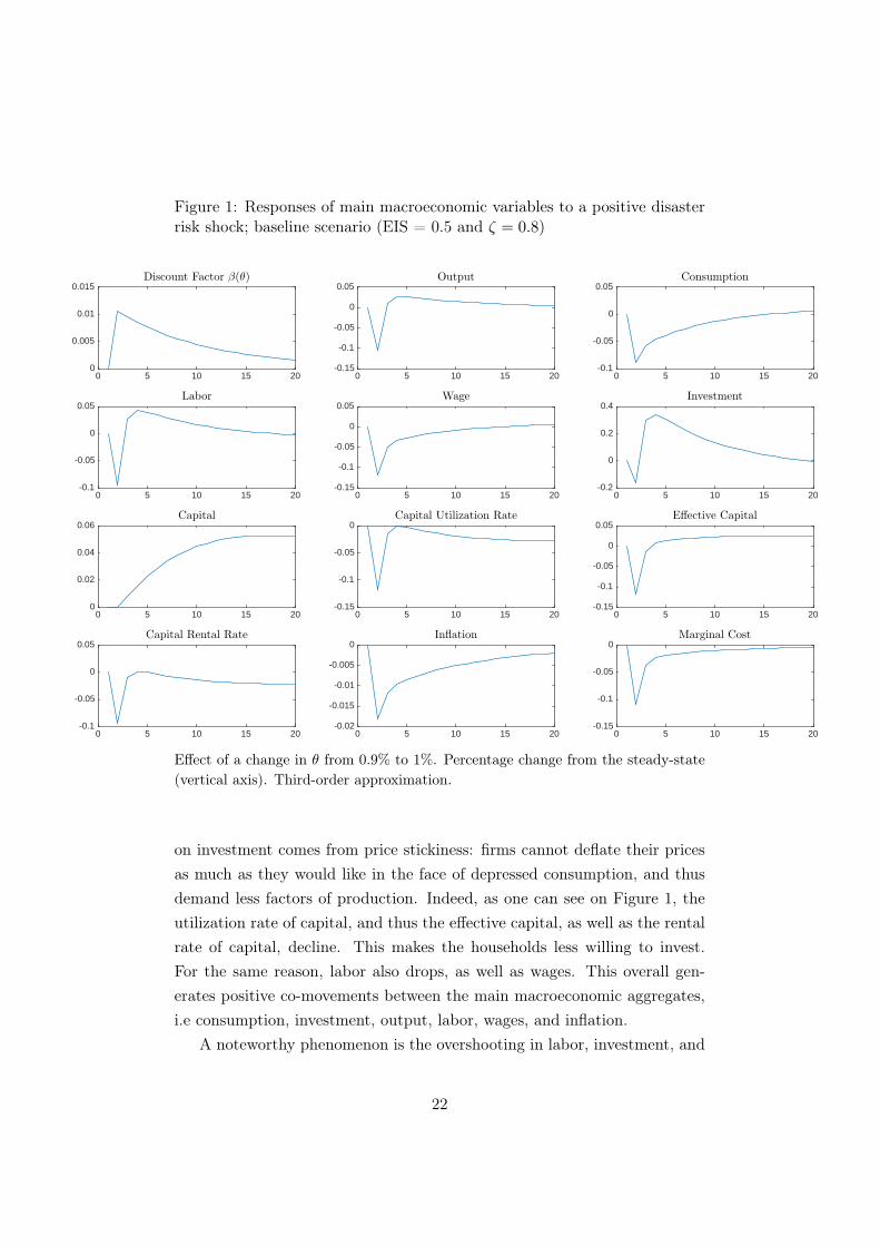
Figure 1: Responses of main macroeconomic variables to a positive disasterrisk shock; baseline scenario (EIS = 0.5 and ζ = 0.8)

0 5 10 15 200

0.005

0.01

0.015Discount Factor β(θ)

0 5 10 15 20-0.15

-0.1

-0.05

0

0.05Output

0 5 10 15 20-0.1

-0.05

0

0.05Consumption

0 5 10 15 20-0.1

-0.05

0

0.05Labor

0 5 10 15 20-0.15

-0.1

-0.05

0

0.05Wage

0 5 10 15 20-0.2

0

0.2

0.4Investment

0 5 10 15 200

0.02

0.04

0.06Capital

0 5 10 15 20-0.15

-0.1

-0.05

0Capital Utilization Rate

0 5 10 15 20-0.15

-0.1

-0.05

0

0.05Effective Capital

0 5 10 15 20-0.1

-0.05

0

0.05Capital Rental Rate

0 5 10 15 20-0.02

-0.015

-0.01

-0.005

0Inflation

0 5 10 15 20-0.15

-0.1

-0.05

0Marginal Cost

Effect of a change in θ from 0.9% to 1%. Percentage change from the steady-state(vertical axis). Third-order approximation.

on investment comes from price stickiness: firms cannot deflate their pricesas much as they would like in the face of depressed consumption, and thusdemand less factors of production. Indeed, as one can see on Figure 1, theutilization rate of capital, and thus the effective capital, as well as the rentalrate of capital, decline. This makes the households less willing to invest.For the same reason, labor also drops, as well as wages. This overall gen-erates positive co-movements between the main macroeconomic aggregates,i.e consumption, investment, output, labor, wages, and inflation.

A noteworthy phenomenon is the overshooting in labor, investment, and

22

to a lower extent in output, in the subsequent periods. Both labor and in-vestment responses are affected by two opposite channels. One is the lowerdemand for factors from firms discussed above. The other is a precaution-ary motive from the households when the disaster risk goes up. Indeed, theagents want to limit the decrease in their consumption by acquiring morecapital and increasing their labor supply when a disaster becomes more likely(under the assumption of an EIS below one). These upward pressures tendto dominate the recessionary effects in the subsequent periods as more andmore firms eventually turn to change their prices.33 This overshooting resultis reminiscent of the uncertainty literature. Indeed, Basu and Bundick (2015)obtain a similar effect from a second-moment discount factor shock in thepresence of sticky prices for instance. This same effect holds in Bloom (2009)although it results from the nonconvex adjustment cost function rather thanprice stickiness in his model. The intuition is similar though in the sense thatfirms enter a zone of “inactivity” as uncertainty shocks hit. Bloom (2009) ar-gues that first-moment shocks generate long-lasting recessions while second-moment shocks indeed typically create sharp but short-lived recessions.

As for asset prices in Figure 2, we observe a ‘flight-to-quality’ effect thatis visible through the drop in the riskfree rate when the disaster risk shockhits,34 as well as an increase in the risk premium. Hence, while improvingGourio (2012)’s predictions for the macroeconomic variables, we preserve thestrength of his mecanism for accounting for the countercyclicality of the riskpremia. We further comment on the relative size of the financial variableresponses with Gourio (2012)’s in the next subsection.

Overall, our results are vey much in line with the preference shocks liter-atures, whether as first- (Smets and Wouters, 2003, for instance) or second-moment ‘uncertainty’ (Basu and Bundick, 2015) effects. This is not sur-prising as β(θ) indeed features a mix of first- and second-moment effects, as

33Another reason amplifying the size of this overshooting is that agents cannot buy anyriskfree asset here, such that risky bonds or risky capital are the only savings vehiclesavailable. That participates in investment bouncing back quite rapidly and strongly afterthe shock. We could relax this assumption and make the bonds riskfree. However, Gourio(2012)’s detrending method could then not be perfectly applied and we would have tocondition our responses on the current state of the economy, within a ‘disaster’ regimeor not, when generating the impule response functions. This would be straightforwardto apply but we chose to present the unconditional impulse response functions, closer toGourio (2012)’s spirit.

34Note again that the riskfree rate is not the interest rate on bonds which are risky inthis model, but merely the inverse of agents’ stochastic discount factor.

23

Figure 2: Responses of main financial variables to a positive disaster riskshock; baseline scenario (EIS = 0.5 and ζ = 0.8)

0 5 10 15 200

0.005

0.01

0.015

0.02Stochastic Discount Factor

0 5 10 15 20

×10-3

-1.5

-1

-0.5

0

0.5

1

1.5

2

2.5Tobin’s q

0 5 10 15 20-0.02

-0.015

-0.01

-0.005

0Riskfree Rate

0 5 10 15 20-0.01

-0.008

-0.006

-0.004

-0.002

0Nominal Rate on (Risky) Bonds

0 5 10 15 20

×10-3

-1

0

1

2

3

4Real Rate on Bonds

0 5 10 15 20

×10-6

0

0.5

1

1.5

2

2.5Risk Premium

Effect of a change in θ from 0.9% to 1%. Percentage change from the steady-state(vertical axis). Third-order approximation.

explained in Gourio (2012). Yet, as long as the EIS was above unity, botheffects played downward: agents become more impatient as the disaster riskshock hits (see next subsection). On the contrary, having an EIS below unitymakes the first- and second-moment effects on β(θ) upward. Combined withprice stickiness, this leads to a recession. In that respect, we reinforce theinterpretation of Gourio (2012)’s mechanism of disaster risk as a potentialsource of preference shifts and uncertainty shocks.

5.2 Effect of a disaster risk shock: other scenarii

In Figures 3 and 4, we consider the same shock under alternative scenarii asfollows:

(i) Flexible prices and EIS = 2, a decentralized version of Gourio (2012)’seconomy, in order to nest his results as a particular case;

24

(ii) Flexible prices and EIS = 0.5 as a value more compatible with thestandard RBC and New Keynesian literatures;

(iii) Sticky prices and EIS = 2, as a mirroring experiment.

Scenario (i) is depicted by the solid line in Figures 3 and 4. This repro-duces the effects of a disaster risk shock in an economy à la Gourio (2012),with flexible prices (ζ = 0) and an EIS of 2, yet here in a decentralized econ-omy version. In contrast with the baseline scenario, an EIS above unity heremakes the agents more impatient (β(θ) decreases) when θ increases. Hence,they save and invest less, driving the economy into a recession, despite anincrease in consumption. Since prices are fully flexible, there is no staggeredeffect on firms’ side, unlike in the previous case. Agents choose to work less,despite precautionary motives at play, since the higher return on today’scapital already sustains their higher consumption level, such that the equi-librium wage increases. This also contrasts with the sticky case where thewage goes down. These results are all identical to Gourio (2012), althoughwithout explicit wage and capital rental rate as for any centralized economy.Among the financial variables in Figure 4, first note that the risk premiumgoes up. The order of magnitude is higher here than in our scenario, but re-call that this holds for an EIS above unity. Moving from an EIS larger thanone to an EIS smaller than one always increases the response of the riskpremium for a given degree of price stickiness/flexibility (comparing scenarii(i) with (ii) on the one hand, and (iii) with baseline, on the other hand).Finally, the riskfree rate goes down here, as in our scenario. However, notethat the drop is more pronounced here, which is a common puzzling featureof finance asset pricing models (Tsai and Wachter, 2015). This suggests thatsticky prices may provide a solution to avoid an excessive fall in the riskfreerate while allowing the EIS to be smaller than one.

Scenario (ii) is depicted by the dashed line in the same figures. Here, weconsider that prices are still flexible, but the EIS is below unity. It turns outthat all macroeconomic responses become the exact opposite of the Gourio(2012)-like solid line. Indeed, the economy enters a boom, driven by thefact that a low EIS increases agents’ propensity to save and thus to invest.Only the stochastic discount factor, the riskfree rate, and the risk premiumresponses, remain qualitatively unchanged in all cases.

25

Figure 3: Responses of main macroeconomic variables to a disaster riskshock; other scenarii (EIS = 2, ζ = 0; EIS = 2, ζ = 0.8, EIS = 0.5, ζ = 0)

0 5 10 15 20-0.01

0

0.01

0.02Discount Factor β(θ)

0 5 10 15 20-0.1

-0.05

0

0.05

0.1Output

0 5 10 15 20-0.05

0

0.05Consumption

0 5 10 15 20-0.1

-0.05

0

0.05

0.1Labor

0 5 10 15 20-0.05

0

0.05

0.1Wage

0 5 10 15 20-1

-0.5

0

0.5

1Investment

0 5 10 15 20-0.1

-0.05

0

0.05

0.1Capital

0 5 10 15 20-0.05

0

0.05

0.1Capital Utilization Rate

0 5 10 15 20-0.05

0

0.05

0.1Effective Capital

0 5 10 15 20-0.05

0

0.05

0.1Capital Rental Rate

0 5 10 15 20-0.2

-0.1

0

0.1

0.2Inflation

0 5 10 15 200

0.02

0.04

0.06

0.08Marginal Cost

ζ=0, EIS=2 (Gourio)ζ=0.8, EIS=2ζ=0, EIS=0.5

Effect of a change in θ from 0.9% to 1%. Percentage change from the steady-state(vertical axis). Third-order approximation.

Scenario (iii) is finally represented with the dotted line. Here, we experi-ment the mirroring combination of sticky prices (as in our baseline) and EISabove unity (as in Gourio (2012)). In that case again, the economy enters aboom, driven by agents’ impatience. As in our baseline scenario, price stick-iness makes all macroeconomic variables co-move, while financial variablespreserve their sign. This case provides an interesting counterfactual exerciseto confirm, on the one hand, the effect of the EIS on the discount factorand the propensity to consume/save, and on the other hand, the fact thataggregate dynamics are more impacted by the demand (supply) side of the

26

Figure 4: Responses of main financial variables to a disaster risk shock; otherscenarii (EIS = 2, ζ = 0; EIS = 2, ζ = 0.8, EIS = 0.5, ζ = 0)

0 5 10 15 200

0.005

0.01

0.015

0.02

0.025Stochastic Discount Factor

0 5 10 15 20

×10-3

-5

-4

-3

-2

-1

0

1

2

3

4

5Tobin’s q

0 5 10 15 20-0.025

-0.02

-0.015

-0.01

-0.005

0Riskfree Rate

0 5 10 15 20-0.025

-0.02

-0.015

-0.01

-0.005

0

0.005

0.01

0.015

0.02Nominal Rate on (Risky) Bonds

0 5 10 15 20

×10-3

-2.5

-2

-1.5

-1

-0.5

0

0.5

1Real Rate on Bonds

0 5 10 15 20

×10-4

0

0.1

0.2

0.3

0.4

0.5

0.6

0.7

0.8

0.9

1Risk Premium

ζ=0, EIS=2 (Gourio)ζ=0.8, EIS=2ζ=0, EIS=0.5

Effect of a change in θ from 0.9% to 1%. Percentage change from the steady-state(vertical axis). Third-order approximation.

economy when price stickiness (flexibility) is at play, for a given value of theEIS. We can also observe that the riskfree rate happens to decrease morethan in the baseline scenario where the EIS was low. This suggests that theasset pricing literature argument of a EIS larger than unity being necessaryto limit the fall of the riskfree rate may not hold under sticky prices.

5.3 Sensitivity analysis

Figure 5 replicates the baseline scenario under alternative values for someother parameters. The qualitative results remain essentially unaffected.

27

The first subfigure presents alternative values for the risk aversion coef-ficient. Our baseline value is standard under Esptein-Zin specification, i.elying typically between 3 and 4. Barro and Jin (2011)’s estimates in thepresence of disaster risk are particularly informative. Yet, we try alternativevalues of γ within the range allowed by the model, i.e compatible with an(endogenous) discount factor β(θ) below unity. When the agents are closerto risk neutrality (γ = 1.5), the upward precautionary labor supply effectcausing the overshooting in labor, investment, and output, turns to be moremoderate. On the contrary, high risk aversion (here, γ = 6) systematicallyamplifies the responses, yet without questioning the qualitative effects.

Next subfigures are related to the fixed part of the discount factor β0

(which would be the standard discount factor in the absence of disasterrisk), the mean disaster size ∆, and the mean probability of disaster θ. Allthree have size but not sign effects.

Only the persistence in disaster risk, ρ, in the last subfigure, seems tohave a qualitative impact on investment. As discussed previously, investmentis driven by two opposite effects and it happens that the upward pressure(the precautionary motive) tends to outweight the downward pressure (firms’lower demand for factors of production) when the persistence is lower. Onceagain, should the households be allowed to buy the riskfree asset in ourmodel setup, this effect may vanish as precautionary savings would findanother vehicle than investment. The size of the subsequent overshooting ishowever negatively correlated with the persistence in disaster risk. Further,this different response of investment is itself not sufficiently strong to modifythe impact response of output to the disaster risk shock.

Finally, Figure 6 displays the responses of selected variables to a mon-etary policy shock under the baseline scenario. These responses are quitestandard and inform us about the validity of the model to well-known shocks.

6 Conclusion

This paper has developed a New Keynesian model featuring a small buttime-varying probability of rare events à la Gourio (2012). In line with theRBC literature, we find that an increase in disaster risk, without occurrenceof the disaster itself, is able to generate a recession and a countercyclical riskpremium. However, the New Keynesian setup improves the RBC responses

28

along two dimensions. First, price stickiness makes the recessionary effectsof disaster risk compatible with a standard value of the elasticity of intertem-poral of substitution below unity, and then also allows consumption, wage,and output prices to co-move as expected. Second, changes in disaster riskthen resemble an increase in agents’ discount factor, instead of a decrease asin Gourio (2012). Indeed, with an EIS below unity, agents (endogenously)become more patient in response to a disaster risk shock. Combined withprice stickiness, the responses of aggregate macroeconomic and financial vari-ables in turn resemble preference shocks (Smets and Wouters (2003), Chris-tiano et al. (2011)) and second-moment “uncertainty” discount factor shock(Basu and Bundick (2015)). In that sense, we show how to conciliate Gourio(2012)’s mechanism of disaster risk with the New Keynesian literatures onpreference and uncertainty shocks.

Preference and uncertainty shocks have lately been praised for pushingthe economy into zero lower bound and secular stagnation situations. To theextent that disaster risk shocks can provide a potential rationale for theseshocks, such an extension could be of interest for further research. Moreover,it could be informative to study variations in the term premium due to thedisaster risk, and interactions between the short-term risk premium with thelong-term end of the yield curve. Finally, it would be worth investigatingthe effectiveness and desirability of policies, such as unconventional monetarypolicies, to be implemented in response to variations in disaster risk.

29

References

[1] Rui Albuquerque, Martin Eichenbaum, Dimitris Papanikolaou, and Ser-gio Rebelo. Long-run bulls and bears. Journal of Monetary Economics,76, Supplement:S21 – S36, 2015.

[2] Martin Andreasen. On the Effects of Rare Disasters and UncertaintyShocks for Risk Premia in Non-Linear DSGE Models. Review of Eco-nomic Dynamics, 15(3):295–316, July 2012.

[3] Orazio P. Attanasio and Martin Browning. Consumption over theLife Cycle and over the Business Cycle. American Economic Review,85(5):1118–37, December 1995.

[4] Scott R. Baker and Nicholas Bloom. Does Uncertainty Reduce Growth?Using Disasters as Natural Experiments. NBER Working Papers 19475,National Bureau of Economic Research, Inc, September 2013.

[5] Ravi Bansal, Dana Kiku, and Amir Yaron. An Empirical Evaluation ofthe Long-Run Risks Model for Asset Prices. Critical Finance Review,1(1):183–221, January 2012.

[6] Ravi Bansal and Amir Yaron. Risks for the long run: A potentialresolution of asset pricing puzzles. The Journal of Finance, 59(4):1481–1509, 2004.

[7] Robert J. Barro. Rare disasters and asset markets in the twentiethcentury. Quarterly Journal of Economics, 2006.

[8] Robert J. Barro. Rare Disasters, Asset Prices, and Welfare Costs. Amer-ican Economic Review, 99(1):243–64, March 2009.

[9] Robert J. Barro and Tao Jin. On the size distribution of macroeconomicdisasters. Econometrica, 79(5):1567–1589, 2011.

[10] Robert J. Barro and Jose F. Ursúa. Consumption disasters in the twen-tieth century. The American Economic Review, pages 58–63, 2008.

[11] Susanto Basu and Brent Bundick. Uncertainty shocks in a model ofeffective demand. Research Working Paper RWP 14-15. November 2014,Revised November 2015., Federal Reserve Bank of Kansas City.

30

[12] Tamim A Bayoumi. Financial Deregulation and Consumption in theUnited Kingdom. The Review of Economics and Statistics, 75(3):536–39, August 1993.

[13] Jason Beeler and John Y. Campbell. The Long-Run Risks Model andAggregate Asset Prices: An Empirical Assessment. Critical FinanceReview, 1(1):141–182, January 2012.

[14] Henk Berkman, Ben Jacobsen, and John B. Lee. Time-varying raredisaster risk and stock returns. Journal of Financial Economics,101(2):313–332, August 2011.

[15] Nicholas Bloom. The Impact of Uncertainty Shocks. Econometrica,77(3):623–685, 05 2009.

[16] Richard Blundell, Martin Browning, and Costas Meghir. Consumer De-mand and the Life-Cycle Allocation of Household Expenditures. Reviewof Economic Studies, 61(1):57–80, January 1994.

[17] Maren Brede. Disaster Risk in a New Keynesian Model. SFB 649Discussion Papers SFB649DP2013-020, Sonderforschungsbereich 649,Humboldt University, Berlin, Germany, April 2013.

[18] Dario Caldara, Jesus Fernández-Villaverde, Juan Rubio-Ramírez, andWen Yao. Computing DSGE Models with Recursive Preferences andStochastic Volatility. Review of Economic Dynamics, 15(2):188–206,April 2012.

[19] John Y Campbell. Bond and Stock Returns in a Simple ExchangeModel. The Quarterly Journal of Economics, 101(4):785–803, November1986.

[20] John Y. Campbell and John Ammer. What Moves the Stock and BondMarkets? A Variance Decomposition for Long-Term Asset Returns. TheJournal of Finance, 48(1):3–37, 1993.

[21] John Y. Campbell and N. Gregory Mankiw. Consumption, Income andInterest Rates: Reinterpreting the Time Series Evidence. In NBERMacroeconomics Annual 1989, Volume 4, NBER Chapters, pages 185–246. National Bureau of Economic Research, Inc, May 1989.

31

[22] Lawrence Christiano, Martin Eichenbaum, and Sergio Rebelo. WhenIs the Government Spending Multiplier Large? Journal of PoliticalEconomy, 119(1):78 – 121, 2011.

[23] John H Cochrane. Presidential address: Discount rates. The Journal ofFinance, 66(4):1047–1108, 2011.

[24] Gauti B. Eggertsson, Andrea Ferrero, and Andrea Raffo. Can structuralreforms help europe? Journal of Monetary Economics, 61:2–22, 2014.

[25] Gauti B. Eggertsson and Michael Woodford. The Zero Bound on Inter-est Rates and Optimal Monetary Policy. Brookings Papers on EconomicActivity, 34(1):139–235, 2003.

[26] Christopher J. Erceg and Jesper Linde. Fiscal Consolidation in an OpenEconomy. American Economic Review, 102(3):186–91, May 2012.

[27] Jesús Fernández-Villaverde and Oren Levintal. Solution methods formodels with rare disasters. Working Paper 21997, National Bureau ofEconomic Research, February 2016.

[28] Jonas D.M. Fisher. On the Structural Interpretation of the Smets-Wouters “Risk Premium” Shock. Journal of Money, Credit and Banking,47(2-3):511–516, 03 2015.

[29] Xavier Gabaix. Variable Rare Disasters: A Tractable Theory of TenPuzzles in Macro-finance. American Economic Review, 98(2):64–67,2008.

[30] Xavier Gabaix. Disasterization: A Simple Way to Fix the Asset Pric-ing Properties of Macroeconomic Models. American Economic Review,101(3):406–09, May 2011.

[31] Xavier Gabaix. Variable Rare Disasters: An Exactly Solved Frameworkfor Ten Puzzles in Macro-Finance. The Quarterly Journal of Economics,127(2):645–700, 2012.

[32] Mark Gertler and Nobuhiro Kiyotaki. Financial Intermediation andCredit Policy in Business Cycle Analysis. In Handbook of MonetaryEconomics, volume 3 of Handbook of Monetary Economics, chapter 11,pages 547–599. Elsevier, 2010.

32

[33] François Gourio. Disaster Risk and Business Cycles. American Eco-nomic Review, 102(6):2734–66, October 2012.

[34] François Gourio. Credit Risk and Disaster Risk. American EconomicJournal: Macroeconomics, 5(3):1–34, July 2013.

[35] Robert E Hall. Intertemporal Substitution in Consumption. Journal ofPolitical Economy, 96(2):339–57, April 1988.

[36] Tomas Havránek, Roman Horvath, Zuzana Irsova, and Marek Rusnak.Cross-country heterogeneity in intertemporal substitution. Journal ofInternational Economics, 96(1):100–118, 2015.

[37] Abigail Hughes and Jumana Saleheen. UK labour productivity since theonset of the crisis ? an international and historical perspective. Bankof England Quarterly Bulletin, 52(2):138–146, 2012.

[38] Alfonso Irarrazabal and Juan Carlos Parra-Alvarez. Time-varying disas-ter risk models: An empirical assessment of the Rietz-Barro hypothesis.CREATES Research Papers 2015-08, School of Economics and Manage-ment, University of Aarhus, February 2015.

[39] Peter N. Ireland. Technology shocks in the new keynesian model. Reviewof Economics and Statistics, 86(4):923–936, 2004.

[40] Marlène Isoré and Urszula Szczerbowicz. Disaster Risk in a New Key-nesian Model. Working Papers 2013-12, CEPII research center, April2013.

[41] Sylvain Leduc and Zheng Liu. Uncertainty Shocks are Aggregate De-mand Shocks. Journal of Monetary Economics, 82:20–35, September2016.

[42] Hayne E. Leland. Saving and Uncertainty: The Precautionary Demandfor Saving. The Quarterly Journal of Economics, 82(3):465–473, August1968.

[43] Sydney Ludvigson. Consumption And Credit: A Model Of Time-Varying Liquidity Constraints. The Review of Economics and Statistics,81(3):434–447, August 1999.

33

[44] Gregory N. Mankiw and Stephen P. Zeldes. The Consumption ofStockholders and Nonstockholders. Journal of Financial Economics,29(1):97–112, 1991.

[45] Roberto Marfè and Julien Penasse. The time-varying risk of macroe-conomic disasters. Technical report, SSRN Working paper, available athttp://ssrn.com/abstract=2773874, 2016.

[46] Rajnish Mehra and Edward C. Prescott. The equity premium: A puzzle.Journal of monetary Economics, 15(2):145–161, 1985.

[47] Stephen Millard and Anamaria Nicolae. The effect of the financial crisison TFP growth: a general equilibrium approach. Bank of Englandworking papers 502, Bank of England, June 2014.

[48] Emi Nakamura, Jón Steinsson, Robert J. Barro, and José Ursúa. Crisesand Recoveries in an Empirical Model of Consumption Disasters. Amer-ican Economic Journal: Macroeconomics, 5(3):35–74, July 2013.

[49] Thomas A. Rietz. The equity risk premium: a solution. Journal ofMonetary Economics, 22(1):117–131, July 1988.

[50] Glenn D. Rudebusch and Eric T. Swanson. The Bond Premium ina DSGE Model with Long-Run Real and Nominal Risks. AmericanEconomic Journal: Macroeconomics, 4(1):105–43, January 2012.

[51] Agnar Sandmo. The Effect of Uncertainty on Saving Decisions. Reviewof Economic Studies, 37(3):353–60, July 1970.

[52] Frank Schorfheide, Dongho Song, and Amir Yaron. Identifying Long-Run Risks: A Bayesian Mixed-Frequency Approach. NBER WorkingPapers 20303, National Bureau of Economic Research, Inc, July 2014.

[53] Emil N. Siriwardane. The probability of rare disasters: Estimation andimplications. Technical report, Harvard Business School Working Paper,2016.

[54] Frank Smets and Rafael Wouters. An Estimated Dynamic StochasticGeneral Equilibrium Model of the EURO Area. Journal of the EuropeanEconomic Association, 1(5):1123–1175, 09 2003.

34

[55] Frank Smets and Rafael Wouters. Shocks and Frictions in US Busi-ness Cycles: A Bayesian DSGE Approach. American Economic Review,97(3):586–606, 2007.

[56] Thomas D. Tallarini Jr. Risk-sensitive real business cycles. Journal ofMonetary Economics, 45(3):507–532, June 2000.

[57] Jerry Tsai and Jessica A. Wachter. Disaster Risk and its Implicationsfor Asset Pricing. NBER Working Papers 20926, National Bureau ofEconomic Research, Inc, February 2015.

[58] Annette Vissing-Jorgensen. Limited Asset Market Participation and theElasticity of Intertemporal Substitution. Journal of Political Economy,110(4):825–853, August 2002.

[59] Jessica A. Wachter. Can time-varying risk of rare disasters explainaggregate stock market volatility? The Journal of Finance, 68(3):987–1035, 2013.

[60] Philippe Weil. The equity premium puzzle and the risk-free rate puzzle.Journal of Monetary Economics, 24(3):401–421, November 1989.

[61] Philippe Weil. Nonexpected utility in macroeconomics. Quarterly Jour-nal of Economics, 105(1):29–42, February 1990.

[62] Wei Yang. Intertemporal Substitution and Equity Premium. Review ofFinance, 20(1):403–445, 2016.

[63] Motohiro Yogo. Estimating the elasticity of intertemporal substitu-tion when instruments are weak. Review of Economics and Statistics,86(3):797–810, 2004.

35

7 Appendices

A Households’ problem with disaster risk

A.1 Utility maximization and first-order conditions

Rewriting the Epstein-Zin preferences

Vt =

[[Ct (1− Lt)$]1−ψ + β0

(EtV

1−γt+1

) 1−ψ1−γ] 1

1−ψ

with the notations Vt = V1

1−ψt and χ = 1− 1−γ

1−ψ as

Vt = [Ct (1− Lt)$]1−ψ + β0

(EtV

1−χt+1

) 11−χ (12)

the Lagrangian for households’ problem reads as

L = [Ct (1− Lt)$]1−ψ + β0

(EtV

1−χt+1

) 11−χ

+ Et

ΛBt

[Wt

ptLt +

Bt(1 + rt−1)

ptext ln(1−∆) +

P ktptutKt +Dt − Ct − It

− Bt+1

pt− Tt

]+ ΛCt

[(1− δ0u

ηt )Kt + S

(ItKt

)Kt −

Kt+1

ext+1 ln(1−∆)

]

with S(ItKt

)= It

Kt− τ

2

(ItKt− I

K

)2the capital adjustment cost function, and

ΛBt and ΛCt the Lagrangian multipliers associated with the budget constraintand capital accumulation constraint, respectively.

The first-order conditions are thus

(Ct :) Et

(ΛBt+1

ΛBt

)=

(Ct+1

Ct

)−ψ (1− Lt+1

1− Lt

)$(1−ψ)

β0

V −χt+1(

EtV1−χt+1

) −χ1−χ

(13)

(Lt :)1− LtCt

=$

W realt

(14)

(Bt+1 :) Et

(ΛBt+1

ΛBt

1 + rt1 + πt+1

ext+1 ln(1−∆)

)= 1 (15)

(ut :)ΛCtΛBt

=P kt /pt

δ0ηuη−1t

(16)

36

(It :)ΛCtΛBt

=1

1− τ(ItKt− I

K

) (17)

(Kt+1 :) Et

ΛBt+1

P kt+1

pt+1ut+1 + ΛCt+1

[1− δ0u

ηt+1 + τ

It+1

Kt+1

(It+1

Kt+1− I

K

)

−τ2

(It+1

Kt+1− I

K

)2]

=ΛCt

Et(ext+1 ln(1−∆))

where ΛCt can be substituted out using (16), such that it is rewritten as

Et

ΛBt+1

ΛBtP k,realt+1

ut+1 +

1

δ0ηuη−1t+1

[1− δ0u

ηt+1 + τ

It+1

Kt+1

(It+1

Kt+1− I

K

)

−τ2

(It+1

Kt+1− I

K

)2]

=P k,realt

δ0ηuη−1t

Et

(1

ext+1 ln(1−∆)

)(18)

or equivalently, using the expression for the Tobin’s q as

Et

ΛBt+1

ΛBt

[P k,realt+1 ut+1

qt+qt+1

qt

[1− δ0u

ηt+1 + τ

It+1

Kt+1

(It+1

Kt+1− I

K

)

−τ2

(It+1

Kt+1− I

K

)2]]

=1

Et(ext+1 ln(1−∆))(19)

A.2 The stochastic discount factor and asset pricing

The stochastic discount factor, Qt,t+1 ≡ ∂Vt/∂Ct+1

∂Vt/∂Ct, is here given by

Qt,t+1 = β0

(Ct+1

Ct

)−ψ (1− Lt+1

1− Lt

)$(1−ψ) V −χt+1

(EtV1−χt+1 )

−χ1−χ

(20)

where Vt = V1

1−ψt and χ = 1 − 1−γ

1−ψ for notational ease, and further from(13),

Qt,t+1 = Et

(ΛBt+1

ΛBt

)(21)

The standard asset pricing orthogonality condition that determines the

37

real return on asset i as Et[Qt,t+1R

it+1

]= 1 here gives

Et

[Qt,t+1R

ft+1

]= 1 (22)

for the riskfree rate, Rf , and

Et(Qt,t+1Rk,realt+1 ) = Et

(ΛBt+1

ΛBtRk,realt+1

)= 1 (23)

for the (real) rate of return on capital, Rk,realt+1 . Using the first-order conditionon capital (18), we can further write

Rk,realt+1 = ext+1 ln(1−∆)Pk,realt+1

P k,realt

δ0ηuη−1t

ut+1 +

1

δ0ηuη−1t+1

[1− δ0u

ηt+1 (24)

+τIt+1

Kt+1

(It+1

Kt+1− I

K

)−τ

2

(It+1

Kt+1− I

K

)2]

or equivalently, using the Tobin’s q notation, as

Rk,realt+1 = ext+1 ln(1−∆)

P k,realt+1 ut+1

qt+qt+1

qt

[1− δ0u

ηt+1

+τIt+1

Kt+1

(It+1

Kt+1− I

K

)−τ

2

(It+1

Kt+1− I

K

)2]

which stresses out the impact of the disaster event on the return on capital.Finally, the risk premium is defined, in gross terms, as the ratio of the realreturn on capital to the riskfree rate, i.e

Et(Premiumt+1) ≡ Et

(Rk,realt+1

Rft+1

)(25)

A.3 Detrending the households’ optimality conditions

In this subsection, we detail our solution method. Following Gourio (2012),it consists in detrending the set of equilibrium equations so as to get rid ofthe disaster event variable xt+1 assuming that the productivity growth is

38

subject to disasters in the same proportion as the assets, i.e.

zt+1

zt= ext+1 ln(1−∆)+µ+εz,t+1 (26)

where xt+1 = 1 with probability θt, and xt+1 = 0 otherwise. This leaves uswith a system where no large shock such as a disaster realization can occur,and thus where perturbations can be used as a solution method to simulateinnovations on the (small) probability of disaster alone.

A.3.1 The utility function

Because of the Epstein-Zin-Weil recursive formulation, the first-order condi-tion on consumption (13) contains the utility function term v, which requiresincluding the utility function as part of the equilibrium set. Following Gou-rio (2012), we here below reexpress the utility function in detrended termsso as to obtain a time-varying discount factor β(θ). First, rewrite (12) as

vt ≡Vt

z1−ψt

= [ct(1− Lt)$]1−ψ +β0

z1−ψt

(Et

(z1−ψt+1 vt+1

)1−χ) 1

1−χ

= [ct(1− Lt)$]1−ψ+β0

z1−ψt

(Et

(z

(1−ψ)t e[µ+εz,t+1+xt+1 ln(1−∆)](1−ψ)vt+1

)1−χ) 1

1−χ

= [ct(1− Lt)$]1−ψ + β0

(Ete

[µ+εz,t+1+xt+1 ln(1−∆)](1−ψ)(1−χ)v1−χt+1

) 11−χ

By independence of the disaster event, the expectation is decomposed as

vt = [ct(1− Lt)$]1−ψ+β0Et

[e(1−γ)xt+1 ln(1−∆)

] 11−χ

e(1−ψ)µEt

[e(1−γ)εz,t+1v1−χ

t+1

] 11−χ

with (1−γ) = (1−ψ)(1−χ) from earlier definition, where the first expectationoperator is conditional on the disaster risk and information at time t whereasthe second expectation operator is only conditional on information at timet. Moreover, since a disaster (x = 1) is realized with probability θ and thereis no disaster (x = 0) otherwise (1− θ), we can further establish that

β0Et

[e(1−γ)xt+1 ln(1−∆)

] 11−χ

= β0

[(1− θt) + θte

(1−γ) ln(1−∆)] 1

1−χ ≡ β(θ)

(27)

39

which defines a time-varying discount factor β(θ) as a function of the (time-varying) disaster risk, and finally allows to rewrite (12) as

vt = [ct(1− Lt)$]1−ψ + β(θt)e(1−ψ)µ

[Ete

(1−γ)εz,t+1v1−χt+1

] 11−χ (28)

A.3.2 The household’s constraints

First, as in Gourio (2012), the law of motion of capital can simply be rewrit-ten in detrended terms as

kt+1 =(1− δt)kt + S

(itkt

)kt

eµ+εz,t+1(29)

where x is not present anymore. On the contrary, for the budget constraintwe obtain

ct + it +bt+1(zt+1/zt)

pt+Ttzt≤ wtptLt +

bt(1 + rt−1)ext ln(1−∆)

pt+P ktptutkt +

Dt

zt

where the term zt+1/zt, and thus the present of disaster is still present, butcan be replaced by the aggregate resource constraint (yt = ct + it) in theequilibrium system.

A.3.3 The stochastic discount factor and FOC on consumption

Applying derivation chain rules, the stochastic discount factor (20) can bereexpressed as

Qt,t+1 =ztzt+1

(ct+1

ct

)−ψ (1− Lt+1

1− Lt

)$(1−ψ)

β(θt)e(1−ψ)µ e(1−γ)εz,t+1v−χt+1[

Ete(1−γ)εz,t+1v1−χt+1

] −χ1−χ

Therefore, by (21), the first-order on consumption becomes

Et

(ΛBt+1

ΛBt

)=

ztzt+1

(ct+1

ct

)−ψ (1− Lt+1

1− Lt

)$(1−ψ)

β(θt)e(1−ψ)µ e(1−γ)εz,t+1v−χt+1[

Ete(1−γ)εz,t+1v1−χt+1

] −χ1−χ

However, since the term zt/zt+1 is not expected but realized here, we needto further define

Qt,t+1 ≡ Qt,t+1zt+1

zt(30)

40

so as to rewrite it as

Et

(ΛBt+1

ΛBt

)=Qt,t+1

Qt,t+1

(ct+1

ct

)−ψ (1− Lt+1

1− Lt

)$(1−ψ)

β(θt)e(1−ψ)µ e(1−γ)εz,t+1v−χt+1[

Ete(1−γ)εz,t+1v1−χt+1

] −χ1−χ

⇔ Qt,t+1 =

(ct+1

ct

)−ψ (1− Lt+1

1− Lt

)$(1−ψ)

β(θt)e(1−ψ)µ e(1−γ)εz,t+1v−χt+1[

Ete(1−γ)εz,t+1v1−χt+1

] −χ1−χ

(31)

A.3.4 Other first-order conditions

The definition of a ‘detrended’ stochastic discount factor (30) further helpsto rewrite the optimality conditions on capital and bonds. Multiplying bothsides of the first-order condition on capital (18) by Et

(ext+1 ln(1−∆)

)and

including it into the same expectation operator by the independence of x,we get

Et

ΛBt+1

ΛBtext+1 ln(1−∆)P k,realt+1

ut+1 +

1

δ0ηuη−1t+1

[1− δ0u

ηt+1 + τ

It+1

Kt+1

(It+1

Kt+1− I

K

)

−τ2

(It+1

Kt+1− I

K

)2]

=P k,realt

δ0ηuη−1t

⇔ Et

ΛBt+1

ΛBt

zt+1

zt

1

eµ+εz,t+1P k,realt+1

ut+1 +

1

δ0ηuη−1t+1

[1− δ0u

ηt+1 + τ

It+1

Kt+1

(It+1

Kt+1− I

K

)

−τ2

(It+1

Kt+1− I

K

)2]

=P k,realt

δ0ηuη−1t

⇔ Et

Qt,t+1P

k,realt+1

ut+1 +

1

δ0ηuη−1t+1

[1− δ0u

ηt+1 + τ

It+1

Kt+1

(It+1

Kt+1− I

K

)

−τ2

(It+1

Kt+1− I

K

)2]

=P k,realt

δ0ηuη−1t

eµ+εz,t+1

41

⇔ Et

Qt,t+1P

k,realt+1

ut+1 +

1

δ0ηuη−1t+1

[1− δ0u

ηt+1 + τ

it+1

kt+1

(it+1

kt+1− i

k

)

−τ2

(it+1

kt+1− i

k

)2]

=P k,realt

δ0ηuη−1t

eµ+εz,t+1 (32)

Given (21), the first-order condition on bonds (15) reads as

Et

(ΛBt+1

ΛBt

1 + rt1 + πt+1

zt+1

zt

)= Et

(Qt,t+1

1 + rt1 + πt+1

)= eµ+εz,t+1 (33)

Finally, it is straightforward to rewrite the first-order conditions on labor(14), capital utilization rate (16), and investment (17), respectively as

1− Ltct

=$

wrealt

(34)

P k,realt

δ0ηuη−1t

=1

1− τ(itkt− i

k

) (35)

1

1− τ(itkt− i

k

) = qt (36)

A.3.5 Asset Pricing

From (30) together with (33), the stochastic discount factor is

Et

(Qt,t+1

)= Et

(Qt,t+1

zt+1

zt

)= Et

(Qt,t+1e

xt,t+1 ln(1−∆)+µ+εz,t+1

)

⇔ Et (Qt,t+1) =Et

(Qt,t+1

)eµ+εz,t+1(1− θt∆)

(37)

such that, by (23), we have the real return on capital as

Rk,realt+1 = (1− θt∆)1 + rt

1 + πt+1(38)

42

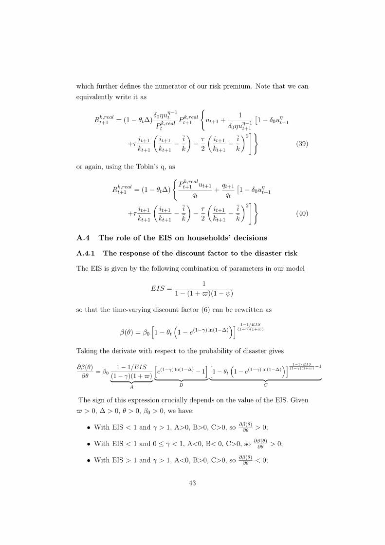
which further defines the numerator of our risk premium. Note that we canequivalently write it as

Rk,realt+1 = (1− θt∆)δ0ηu

η−1t

P k,realt

P k,realt+1

ut+1 +

1

δ0ηuη−1t+1

[1− δ0u

ηt+1

+τit+1

kt+1

(it+1

kt+1− i

k

)− τ

2

(it+1

kt+1− i

k

)2]

(39)

or again, using the Tobin’s q, as

Rk,realt+1 = (1− θt∆)

P k,realt+1 ut+1

qt+qt+1

qt

[1− δ0u

ηt+1

+τit+1

kt+1

(it+1

kt+1− i

k

)− τ

2

(it+1

kt+1− i

k

)2]

(40)

A.4 The role of the EIS on households’ decisions

A.4.1 The response of the discount factor to the disaster risk

The EIS is given by the following combination of parameters in our model

EIS =1

1− (1 +$)(1− ψ)

so that the time-varying discount factor (6) can be rewritten as

β(θ) = β0

[1− θt

(1− e(1−γ) ln(1−∆)

)] 1−1/EIS(1−γ)(1+$)

Taking the derivate with respect to the probability of disaster gives

∂β(θ)

∂θ= β0

1− 1/EIS

(1− γ)(1 +$)︸ ︷︷ ︸A

[e(1−γ) ln(1−∆) − 1

]︸ ︷︷ ︸

B

[1− θt

(1− e(1−γ) ln(1−∆)

)] 1−1/EIS(1−γ)(1+$)

−1

︸ ︷︷ ︸C

The sign of this expression crucially depends on the value of the EIS. Given$ > 0, ∆ > 0, θ > 0, β0 > 0, we have:

• With EIS < 1 and γ > 1, A>0, B>0, C>0, so ∂β(θ)∂θ > 0;

• With EIS < 1 and 0 ≤ γ < 1, A<0, B< 0, C>0, so ∂β(θ)∂θ > 0;

• With EIS > 1 and γ > 1, A<0, B>0, C>0, so ∂β(θ)∂θ < 0;

43

• With EIS > 1 and 0 ≤ γ < 1, A>0, B<0, C>0, so ∂β(θ)∂θ < 0;

• With limEIS→1∂β(θ)∂θ → 0.

Overall, an increase in the probability of disaster makes agents more patient(higher β(θ)) when the EIS is below unity, and inversely, more impatient(lower β(θ)) when the EIS is above unity. This holds for all degrees of riskaversion (all values of γ), including risk neutrality.

A.4.2 The response of the riskfree rate to the disaster risk (alongthe balanced growth path)

Along the balanced growth path, the riskfree rate is given by

Rf =

[1− θ

(1− e(1−γ) ln(1−∆)

)]$(1−γ)+1/EIS−γ(1+$)(1−γ)

β0e−µ$+1/EIS

1+$[1− θ

(1− e−γ ln(1−∆)

)]The derivative ∂Rf/∂θ is always negative, i.e the riskfree rate decreases inthe disaster risk for all values of the EIS and risk aversion. However, themagnitude of the slump is sensitive to the value of the EIS: the riskfree ratedecreases more with the disaster risk for an EIS below unity than for an EISabove unity, given the degree of risk aversion (including risk neutrality). Forinstance, with the baseline calibration we find

• With EIS = 0.5 and γ = 3.8, ∂Rf

∂θ ≈ −0.666;

• With EIS = 2 and γ = 3.8, ∂Rf

∂θ ≈ −0.504;

• With EIS = 0.5 and γ = 0.5, ∂Rf

∂θ ≈ −0.324;

• With EIS = 2 and γ = 0.5, ∂Rf

∂θ ≈ −0.217;

• With EIS = 0.5 and γ = 0, ∂Rf

∂θ ≈ −0.291;

• With EIS = 2 and γ = 0, ∂Rf

∂θ ≈ −0.190

Note again that this is not a general equilibrium effect.

44

A.4.3 The response of the return on capital to the disaster risk(along the balanced growth path)

Along the balanced growth path, the return on capital is given by

Rk =1− θ

(1− eln(1−∆)

)β0e−µ$+1/EIS

1+$[1− θ

(1− e(1−γ) ln(1−∆)

)] 1−1/EIS(1−γ)(1+$)

The derivative ∂Rk/∂θ is also always negative, i.e the rate of return oncapital decreases in the disaster risk. However, just as for the riskfree rate,the decrease is larger when the EIS is below unity (rather than above), forall values of risk aversion (including risk neutrality). For instance, we have

• With EIS = 0.5 and γ = 3.8, ∂Rk

∂θ ≈ −0.332;

• With EIS = 2 and γ = 3.8, ∂Rk

∂θ ≈ −0.169;

• With EIS = 0.5 and γ = 0.5, ∂Rk

∂θ ≈ −0.295;

• With EIS = 2 and γ = 0.5, ∂Rk

∂θ ≈ −0.188;

• With EIS = 0.5 and γ = 0, ∂Rk

∂θ ≈ −0.291;

• With EIS = 2 and γ = 0, ∂Rk

∂θ ≈ −0.190

A.4.4 The response of the risk premium to the disaster risk (alongthe balanced growth path)

Finally, along the balanced growth path, the risk premium is given by

Premium =

[1− θ

(1− eln(1−∆)

)] [1− θ

(1− e−γ ln(1−∆)

)]1− θ

(1− e(1−γ) ln(1−∆)

)The derivative, calculated under our calibration values, gives

• With γ = 3.8, ∂E(Rk)/Rf

∂θ ≈ 0.333;

• With γ = 0.5, ∂E(Rk)/Rf

∂θ ≈ 0.029;

• With γ = 0, ∂E(Rk)/Rf

∂θ = 0.

The risk premium reacts positively to the disaster risk, and the larger therisk aversion the larger its magnitude. It does not directly depend on the

45

value of the EIS along the balanced growth path, in line with Gourio (2012).However, in general equilibrium, the EIS plays a qualitative role: the largerthe EIS, the smaller the risk premium in response to the disaster risk shock(comparing the impulse response functions from Figures 1 to 4).

B Firms’ problem

B.1 Production aggregation

The aggregate of intermediate goods is given by

Yt =

(∫ 1

0Y

ν−1ν

j,t dj

) νν−1

so that the representative firm in the final sector maximizes profits as

maxYt,j

pt

(∫ 1

0Y

ν−1ν

j,t dj

) νν−1

−∫ 1

0pj,tYj,tdj

The first-order condition with respect to Yt,j yields a downward sloping de-mand curve for each intermediate good j as

Yj,t =

(pj,tpt

)−νYt

The nominal value of the final good is the sum of prices times quantities ofintermediates

ptYt =

∫ 1

0pj,tYj,tdj

in which Yt is substituted to give the aggregate price index as

pt =

(∫ 1

0p1−νj,t dj

) 11−ν

B.2 Cost minimization

Firms are price-takers in the input markets, facing (non-detrended) nominalwage Wnom

t and capital rental rate P kt . They choose the optimal quantitiesof labor and capital given the input prices and subject to the restriction ofproducing at least as much as the intermediate good is demanded at the

46

given price. The intra-temporal problem is thus

minLj,t,Kj,t

WtLj,t + P kt Kj,t

s.t. Kαj,t(ztLj,t)

1−α ≥(pj,tpt

)−νYt

The (detrended) first-order conditions are

(Lj,t :) wt = mcnomj,t (1− α)

(kj,tLj,t

)α

(Kj,t :) P kt = mcnomj,t α

(kj,tLj,t

)α−1

in which the Lagrange multiplier denoted mcnomj,t can be interpreted as the(nominal) marginal cost associated with an additional unit of capital or labor.Rearranging gives the optimal capital over labor ratio as(

kj,tLj,t

)∗=wt

P kt

α

(1− α)

in which none of the terms on the right hand side depends on j, and thusholds for all firms in equilibrium, i.e., kt

Lt=

kj,tLj,t

. Replacing in one of thefirst-order conditions above gives

mcnom∗t =

(P ktα

)α(wt

1− α

)1−α

Reexpressing in real terms mc∗t = mcnom∗t /pt, we finally have

mc∗t =

(P k,realt

α

)α(wrealt

1− α

)1−α

where P k,real and wreal are the real capital rental rate and (detrended) wage.

B.3 Profit maximization

Let us now consider the pricing problem of a firm that gets to update itsprice in period t and wants to maximize the present discounted value of

47

future profits. The (nominal) profit flows read as

pj,tYj,t −WtLj,t − P kj,tKj,t = (pj,t −mcnomt )Yj,t

which can be reexpressed in real terms as pj,tptYj,t − mc∗tYj,t. These profit

flows are discounted by both the stochastic discount factor, Qt,t+s, and bythe probability ζs that a price chosen at time t is still in effect at time s.Finally, given Yj,t =

(pj,tpt

)−νYt, the maximization problem is thus

maxpj,t

Et

∞∑s=0

(ζ)sQt+s

((pj,tpt+s

)1−νYt+s −mc∗t+s

(pj,tpt+s

)−νYt+s

)

which can be further simplified, using mc∗t =mcnomtpt

and factorizing, as

maxpj,t

Et

∞∑s=0

(ζ)sQt+spν−1t+s Yt+s

(p1−νj,t −mc

nomt p−νj,t

)The first-order condition is then

Et

∞∑s=0

(ζ)sQt+spν−1t+s Yt+s

((1− ν)p−νj,t + ν mcnomt p−ν−1

j,t

)= 0

which simplifies as

p∗j,t =ν

ν − 1Et

∑∞s=0 (ζ)sQt+sp

νt+sYt+smc

∗t+s∑∞

s=0 (ζ)sQt+spν−1t+s Yt+s

Note that this optimal price depends on aggregate variables only, so thatp∗t = p∗j,t. Expressed as a ratio over the current price, we thus have

p∗tpt

=ν

ν − 1Et

∑∞s=0 (ζ)sQt+s

(pt+spt

)νYt+smc

∗t+s∑∞

s=0 (ζ)sQt+s

(pt+spt

)ν−1Yt+s

which can be written recursively as

p∗tpt

=ν

ν − 1Et

Ξ1t

Ξ2t

with

Ξ1t = Ytmc∗t + ζEtQt,t+1

(pt+1

pt

)νΞ1t+1

48

Ξ2t = Yt + ζEtQt,t+1

(pt+1

pt

)ν−1

Ξ2t+1

Replacing Qt,t+1 ≡ Qt,t+1ztzt+1

, and detrending, these are simplified as

Ξ1t = ytmc∗t + ζEtQt,t+1

(pt+1

pt

)νΞ1t+1 (41)

Ξ2t = yt + ζEtQt,t+1

(pt+1

pt

)ν−1

Ξ2t+1 (42)

where Ξt ≡ Ξt/zt, the detrended variable.

C Aggregation

C.1 Bonds market

Market-clearing requires the public debt to equate the quantity of bondspurchased by the households at each time, i.e Debtt = Bt, therefore makingthe public debt symmetrically affected by disasters. Moreover, we assumethat the public budget has to be balanced every period, i.e the sum of taxrevenues and new debt issuance must be equal to the current debt issuanceto be repaid with interest rates (as for the non-disaster part), i.e

Ttpt +Bt+1 = [Bt(1 + rt−1)]ext+1 ln(1−∆)

or, in detrended terms,

Ttzt

+bt+1

pt=bt(1 + rt−1)

pteµ+εz,t+1

C.2 Aggregate demand

Replacing the tax level above into the household’s budget constraint gives

ct+it+

(bt(1 + rt−1)

pteµ+εz,t+1− bt+1

pt

)= wrealt Lt+

(bt(1 + rt−1)

pteµ+εz,t+1− bt+1

pt

)+P k,realt utkt+

Dt

zt

which just simplifies as

ct + it = wrealt Lt + P k,realt kt +Dt

zt

49

i.e, in non-detrended terms, as

Ct + It = W realt Lt + P k,realt Kt +Dt

where we now have to verify that the RHS is equal to Yt. Total dividends(or profits) Dt must be equal to the sum of dividends (or profits) fromintermediate good firms, i.e

Dt =

∫ 1

0Dj,tdj

The (real) dividends (or profits) from intermediate good firms j are given by

Dj,t =pj,tptYj,t −W real

t Lj,t − P k,realt Kj,t

Substituting Yj,t, we have

Dj,t =

(pj,tpt

)1−νYt −W real

t Lj,t − P k,realt Kj,t

Therefore, knowing that Dt(real) =∫ 1

0 Dj,t(real)dj, we get

Dt =

∫ 1

0

((pj,tpt

)1−ν

Yt −W realt Lj,t − P k,realt Kj,t

)dj =

∫ 1

0

(pj,tpt

)1−ν

Ytdj

−∫ 1

0

W realt Lj,tdj −

∫ 1

0

P k,realt Kj,tdj

Dt =

∫ 1

0

((pj,tpt

)1−ν

Yt −W realt Lj,t − P k,realt Kj,t

)dj = Yt

1

p1−νt

∫ 1

0

(pj,t)1−ν

dj

−W realt

∫ 1

0

Lj,tdj − P k,realt

∫ 1

0

Kj,tdj

Given that (i) the aggregate price level is p1−νt =

∫ 10 p

1−νj,t dj, (ii) aggregate

labor demand must equal supply, i.e∫ 1

0 Lj,tdj = Lt, and (iii) aggregatesupply of capital services must equal demand

∫ 10 Kj,tdj = Kt, the aggregate

(real) dividend (or profit) is

Dt = Yt −W realt Lt − P k,realt Kt

50

Replaced into the household’s budget constraint, this finally gives the aggre-gate accounting identity as

Yt = Ct + It

or in detrended termsyt = ct + it

C.3 Inflation

Firms have a probability 1− ζ of getting to update their price each period.Since there are an infinite number of firms, there is also the exact fraction1− ζ of total firms who adjust their prices and the fraction ζ who stay withthe previous period price. Moreover, since there is a random sampling fromthe entire distribution of firm prices, the distribution of any subset of firmprices is similar to the entire distribution. Therefore, the aggregate priceindex, p1−ν

t =∫ 1

0 p1−νj,t dj, is rewritten as

p1−νt =

∫ 1−ζ

0p∗1−νt dj +

∫ 1

1−ζp1−νj,t−1dj

which simplifies asp1−νt = (1− ζ)p∗1−νt + ζp1−ν

t−1

Let us divide both sides of the equation by p1−νt−1(

ptpt−1

)1−ν= (1− ζ)

(p∗tpt−1

)1−ν+ ζ

(pt−1

pt−1

)1−ν

and define the gross inflation rate as

1 + πt ≡ptpt−1

and the gross reset inflation rate as

1 + π∗t ≡p∗tpt−1

we get(1 + πt)

1−ν = (1− ζ)(1 + π∗t )1−ν + ζ

51

Finally, since we know that

p∗tpt

=ν

ν − 1Et

Ξ1t

Ξ2t

we have the reset inflation rate as

(1 + π∗t ) = (1 + πt)ν

ν − 1Et

Ξ1t

Ξ2t

with the expressions given previously for Ξ1 and Ξ2 (see Appendix B.3), orequivalently with the detrended terms as

(1 + π∗t ) = (1 + πt)ν

ν − 1Et

Ξ1t

Ξ2t

C.4 Aggregate supply

We know that the demand to individual firm j is given by

Yj,t =

(pj,tpt

)−νYt

and that firm j hires labor and capital in the same proportion as the aggre-gate capital to labor ratio (common factor markets). Hence, substituting inthe production function for the intermediate good j we get(

Kt

ztLt

)αztLj,t =

(pj,tpt

)−νYt

which can be rewritten with detrended variables as(ktLt

)αLj,t =

(pj,tpt

)−νyt

Then, summing up across the intermediate firms gives(ktLt

)α ∫ 1

0Lj,tdj = yt

∫ 1

0

(pj,tpt

)−νdj

52

Given that aggregate labor demand and supply must equal, i.e∫ 1

0 Lj,tdj = Lt,we have ∫ 1

0

(pj,tpt

)−νdjyt = kαt L

1−αt

Thus, the aggregate production function can be written as

yt =kαt L

1−αt

Ωt

where Ωt =∫ 1

0

(pj,tpt

)−νdj measures a distortion introduced by the disper-

sion in relative prices.35 In order to express Ωt in aggregate terms, let usdecompose it according to the Calvo pricing assumption again, so that

Ωt =

∫ 1

0

(pj,tpt

)−νdj = pνt

∫ 1

0p−νj,t

pνt

∫ 1

0p−νj,t = pνt

(∫ 1−ζ

0p∗−νt dj +

∫ 1

1−ζp−νj,t−1dj

)

pνt

∫ 1

0p−νj,t = pνt (1− ζ)p∗−νt + pνt

∫ 1

1−ζp−νj,t−1dj

pνt

∫ 1

0p−νj,t = (1− ζ)

(p∗tpt

)−ν+ pνt

∫ 1

1−ζp−νj,t−1dj

pνt

∫ 1

0p−νj,t = (1− ζ)

(p∗tpt−1

)−ν (pt−1

pt

)−ν+ pνt

∫ 1

1−ζp−νj,t−1dj

pνt

∫ 1

0p−νj,t = (1− ζ)(1 + π∗t )

−ν(1 + πt)ν + p−νt−1p

νt

∫ 1

1−ζ

(pj,t−1

pt−1

)−νdj

Given random sampling and the fact that there is a continuum of firms

Ωt = (1− ζ)(1 + π∗t )−ν(1 + πt)

ν + ζ(1 + πt)νΩt−1

D Full set of equilibrium conditions

Processus for the disaster risk

log θt = (1− ρθ) log θ + ρθ log θt−1 + σθεθt (43)35This distortion is not the one associated with the monopoly power of firms but an

additional one that arises from the relative price fluctuations due to prie stickiness.

53

Time-varying discount factor

β(θ) = β0

[1− θt + θte

(1−γ) ln(1−∆)] 1

1−χ (44)

Households

Qt,t+1 =

(ct+1

ct

)−ψ (1− Lt+1

1− Lt

)$(1−ψ)

β(θt)e(1−ψ)µ e(1−γ)εz,t+1v−χt+1[

Ete(1−γ)εz,t+1v1−χt+1

] −χ1−χ

(45)

1− Ltct

=$

wrealt

(46)

Et

(Qt,t+1

1 + rt1 + πt+1

)= eµ+εz,t+1 (47)

P k,realt

δ0ηuη−1t

=1

1− τ(itkt− i

k

) (48)

1

1− τ(itkt− i

k

) = qt (49)

Et

Qt,t+1P

k,realt+1

ut+1 +

1

δ0ηuη−1t+1

[1− δ0u

ηt+1 + τ

it+1

kt+1

(it+1

kt+1− i

k

)

−τ2

(it+1

kt+1− i

k

)2]

=P k,realt

δ0ηuη−1t

eµ+εz,t+1 (50)

vt = [ct(1− Lt)$]1−ψ + β(θt)e(1−ψ)µEt

[e(1−ψ)(1−χ)εz,t+1v1−χ

t+1

] 11−χ (51)

kt+1 =(1− δt)kt + S

(itkt

)kt

eµ+εz,t+1(52)

Asset pricing

Qt,t+1 =Qt,t+1

eµ+εz,t+1(1− θt∆)(53)

54

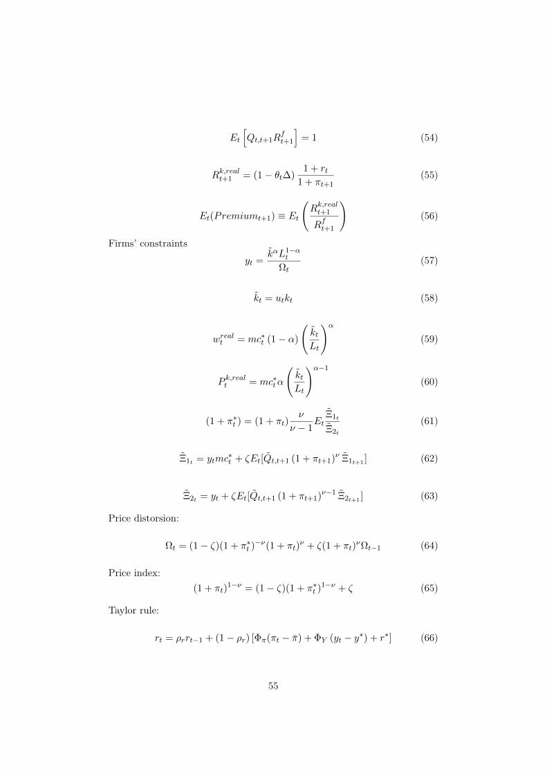
Et

[Qt,t+1R

ft+1

]= 1 (54)

Rk,realt+1 = (1− θt∆)1 + rt

1 + πt+1(55)

Et(Premiumt+1) ≡ Et

(Rk,realt+1

Rft+1

)(56)

Firms’ constraints

yt =kαL1−α

t

Ωt(57)

kt = utkt (58)

wrealt = mc∗t (1− α)

(ktLt

)α(59)

P k,realt = mc∗tα

(ktLt

)α−1

(60)

(1 + π∗t ) = (1 + πt)ν

ν − 1Et

Ξ1t

Ξ2t

(61)

Ξ1t = ytmc∗t + ζEt[Qt,t+1 (1 + πt+1)ν Ξ1t+1 ] (62)

Ξ2t = yt + ζEt[Qt,t+1 (1 + πt+1)ν−1 Ξ2t+1 ] (63)

Price distorsion:

Ωt = (1− ζ)(1 + π∗t )−ν(1 + πt)

ν + ζ(1 + πt)νΩt−1 (64)

Price index:(1 + πt)

1−ν = (1− ζ)(1 + π∗t )1−ν + ζ (65)

Taylor rule:

rt = ρrrt−1 + (1− ρr) [Φπ(πt − π) + ΦY (yt − y∗) + r∗] (66)

55

Aggregate resource constraint:

yt = ct + it (67)

This is a system of 25 equations in 25 unknowns:θ, β(θ), y, c, i, L, k, k, u, Q,

Q,Rk,real, Rf , P remium,P k,real, wreal, q,Ω, π, π∗, Ξ1, Ξ2,mc∗, v, r

. The re-

sponses to a disaster risk shock are computed with a third-order approxima-tion around its steady-state using Dynare.

56

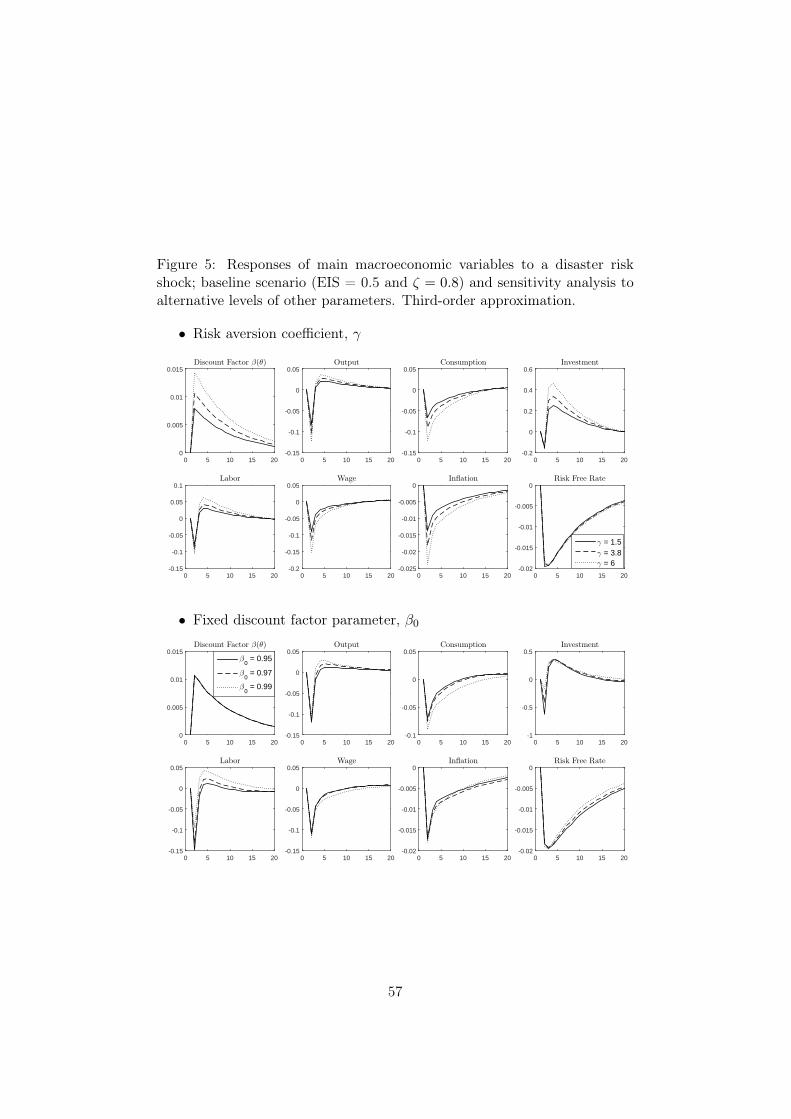
Figure 5: Responses of main macroeconomic variables to a disaster riskshock; baseline scenario (EIS = 0.5 and ζ = 0.8) and sensitivity analysis toalternative levels of other parameters. Third-order approximation.

• Risk aversion coefficient, γ

0 5 10 15 200

0.005

0.01

0.015Discount Factor β(θ)

0 5 10 15 20-0.15

-0.1

-0.05

0

0.05Output

0 5 10 15 20-0.15

-0.1

-0.05

0

0.05Consumption

0 5 10 15 20-0.2

0

0.2

0.4

0.6Investment

0 5 10 15 20-0.15

-0.1

-0.05

0

0.05

0.1Labor

0 5 10 15 20-0.2

-0.15

-0.1

-0.05

0

0.05Wage

0 5 10 15 20-0.025

-0.02

-0.015

-0.01

-0.005

0Inflation

0 5 10 15 20-0.02

-0.015

-0.01

-0.005

0Risk Free Rate

γ = 1.5γ = 3.8γ = 6

• Fixed discount factor parameter, β0

0 5 10 15 200

0.005

0.01

0.015Discount Factor β(θ)

0 5 10 15 20-0.15

-0.1

-0.05

0

0.05Output

0 5 10 15 20-0.1

-0.05

0

0.05Consumption

0 5 10 15 20-1

-0.5

0

0.5Investment

0 5 10 15 20-0.15

-0.1

-0.05

0

0.05Labor

0 5 10 15 20-0.15

-0.1

-0.05

0

0.05Wage

0 5 10 15 20-0.02

-0.015

-0.01

-0.005

0Inflation

0 5 10 15 20-0.02

-0.015

-0.01

-0.005

0Risk Free Rate

β0 = 0.95

β0 = 0.97

β0 = 0.99

57

• Steady-state probability of disaster, θ

0 5 10 15 200

0.005

0.01

0.015Discount Factor β(θ)

0 5 10 15 20-0.15

-0.1

-0.05

0

0.05Output

0 5 10 15 20-0.1

-0.05

0

0.05Consumption

0 5 10 15 20-0.2

0

0.2

0.4Investment

0 5 10 15 20-0.1

-0.05

0

0.05Labor

0 5 10 15 20-0.15

-0.1

-0.05

0

0.05Wage

0 5 10 15 20-0.02

-0.015

-0.01

-0.005

0Inflation

0 5 10 15 20

×10-3

-20

-15

-10

-5

0

5Risk Free Rate

θ=0.4%

θ=0.72%

θ=0.9%

• Size of disaster, ∆

0 5 10 15 200

0.005

0.01

0.015

0.02Discount Factor β(θ)

0 5 10 15 20-0.15

-0.1

-0.05

0

0.05Output

0 5 10 15 20-0.2

-0.15

-0.1

-0.05

0

0.05Consumption

0 5 10 15 20-0.2

0

0.2

0.4

0.6Investment

0 5 10 15 20-0.15

-0.1

-0.05

0

0.05

0.1Labor

0 5 10 15 20-0.2

-0.15

-0.1

-0.05

0

0.05Wage

0 5 10 15 20-0.03

-0.02

-0.01

0

0.01Inflation

0 5 10 15 20-0.03

-0.02

-0.01

0Risk Free Rate

∆=0.15∆=0.22∆=0.3

• Persistence of disaster probability, ρθ

0 5 10 15 200

0.005

0.01

0.015Discount Factor β(θ)

0 5 10 15 20-0.15

-0.1

-0.05

0

0.05Output

0 5 10 15 20-0.1

-0.05

0

0.05Consumption

0 5 10 15 20-0.2

0

0.2

0.4Investment

0 5 10 15 20-0.1

-0.05

0

0.05Labor

0 5 10 15 20-0.15

-0.1

-0.05

0

0.05Wage

0 5 10 15 20

×10-3

-20

-15

-10

-5

0

5Inflation

0 5 10 15 20-0.03

-0.02

-0.01

0

0.01Risk Free Rate

ρθ = 0

ρθ = 0.75

ρθ = 0.9

58

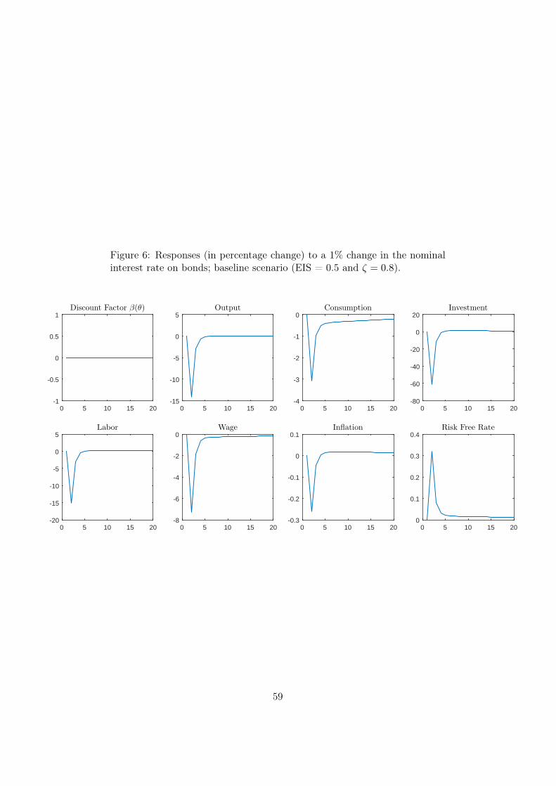
Figure 6: Responses (in percentage change) to a 1% change in the nominalinterest rate on bonds; baseline scenario (EIS = 0.5 and ζ = 0.8).

0 5 10 15 20-1

-0.5

0

0.5

1Discount Factor β(θ)

0 5 10 15 20-15

-10

-5

0

5Output

0 5 10 15 20-4

-3

-2

-1

0Consumption

0 5 10 15 20-80

-60

-40

-20

0

20Investment

0 5 10 15 20-20

-15

-10

-5

0

5Labor

0 5 10 15 20-8

-6

-4

-2

0Wage

0 5 10 15 20-0.3

-0.2

-0.1

0

0.1Inflation

0 5 10 15 200

0.1

0.2

0.3

0.4Risk Free Rate

59

Documents de Travail

600. M. Mogliani and T. Ferrière, “Rationality of announcements, business cycle asymmetry, and predictability of revisions. The case of French GDP” September 2016

601. R. S.J. Koijen; F. Koulischer; B. Nguyen and M. Yogo, “Quantitative Easing in the Euro Area: The Dynamics of

Risk Exposures and the Impact on Asset Prices” September 2016

602. O. de Bandt and M. Chahad, “A DGSE Model to Assess the Post-Crisis Regulation of Universal Banks” September 2016

603. C. Malgouyres, “The Impact of Chinese Import Competition on the Local Structure of Employment and Wages:

Evidence from France” September 2016

604. G. Cette, J. Lopez and J. Mairesse, “Labour market regulations and capital labour substitution” October 2016

605. C. Hémet and C. Malgouyres, “Diversity and Employment Prospects: Neighbors Matter!” October 2016

606. M. Ben Salem and B. Castelletti-Font, “Which combination of fiscal and external imbalances to determine the long-run dynamics of sovereign bond yields?” November 2016

607. M. Joëts, V. Mignon and T. Razafindrabe, “Does the volatility of commodity prices reflect macroeconomic

uncertainty?” November 2016

608. M. Bussière, G. Gaulier and W. Steingress, “Global Trade Flows: Revisiting the Exchange Rate Elasticities” November 2016

609. V.Coudert and J. Idier, “An Early Warning System for Macro-prudential Policy in France” November 2016

610. S. Guilloux-Nefussi, “Globalization, Market Structure and Inflation Dynamics” December 2016

611. S.Fries, J-S. Mésonnier, S. Mouabbi, and J-P. Renne, “National natural rates of interest and the single monetary

policy in the Euro Area” December 2016

612. J. Blaum, C. Lelarge and M. Peters, “The Gains from Input Trade with Heterogeneous Importers” December 2016

613. A. Penalver, “Optimal Monitoring of Long-Term Loan Contracts” December 2016

614. M. Isoré and U. Szczerbowicz, “Disaster Risk and Preference Shifts in a New Keynesian Model” December 2016

Pour accéder à la liste complète des Documents de Travail publiés par la Banque de France veuillez consulter le site : www.banque-france.fr For a complete list of Working Papers published by the Banque de France, please visit the website: www.banque-france.fr Pour tous commentaires ou demandes sur les Documents de Travail, contacter la bibliothèque de la Direction Générale des Études et des Relations Internationales à l'adresse suivante : For any comment or enquiries on the Working Papers, contact the library of the Directorate General Economics and International Relations at the following address : BANQUE DE FRANCE 49- 1404 Labolog 75049 Paris Cedex 01 tél : 0033 (0)1 42 97 77 24 ou 01 42 92 63 40 ou 48 90 ou 69 81 email : 1404-ut@banque-france.fr