directory - lamar.educs.lamar.edu/faculty/osborne/5369/sum05/eer-report.pdf · · 2008-06-19......
TRANSCRIPT

COSC 5369, Graduate Project, Energy Efficient Routing
Directory
ABSTRACT.................................................................................................................................... 1 Chapter 1: Introduction................................................................................................................... 2
1.1 Sensor and Wireless Sensor Network (WSNs) Overview............................................................... 2 1.2 Project purpose and motivation....................................................................................................... 2 1.3 Project overview ............................................................................................................................. 3 1.4 Report Outline................................................................................................................................. 3
Chapter 2: Current Routing Protocols in WSNs............................................................................. 5 2.1 Based on Network Topology........................................................................................................... 5
2.1.1 Flat-based Routing ............................................................................................................... 5 2.1.2 Hierarchical Routing ............................................................................................................ 6 2.1.3 Location based Routing Protocols ....................................................................................... 8
2.2 Routing Protocol based on Protocol Operation............................................................................... 8 2.3 Relationship Between the New Protocol and the Existing Protocols.............................................. 9
Chapter 3: An Ideal Algorithm...................................................................................................... 10 3.1 Current Energy Saving Mechanisms for WSNs............................................................................ 10 3.2 Target Network Model of The New Algorithm............................................................................. 10 3.3 Most Energy Efficient Region ...................................................................................................... 11
3.3.1 Relay Node......................................................................................................................... 11 3.3.2 Shape of the most energy efficient region.......................................................................... 14 3.3.3 Algorithm for computing MEER ....................................................................................... 16 3.3.4 Implementation Issues........................................................................................................ 16
Chapter 4: Practical Algorithm ..................................................................................................... 18 4.1 Design Issues ................................................................................................................................ 18
4.1.1 Node lifetime...................................................................................................................... 18 4.1.2 Network lifetime ................................................................................................................ 18 4.1.3 Node deployment ............................................................................................................... 19 4.1.4 Data reporting model ......................................................................................................... 19 4.1.5 Detection of minimal transmission power to the neighbors............................................... 19 4.1.5 Naming............................................................................................................................... 20
4.2 Algorithm Design.......................................................................................................................... 20 4.2.1 Algorithm ........................................................................................................................... 22 4.2.2 Proof................................................................................................................................... 23
4.3 Algorithm Analysis ....................................................................................................................... 24 4.3.1 What is the advantage of the algorithm?............................................................................ 24 4.3.2 Constructing time............................................................................................................... 24 4.3.3 Cost of probing process...................................................................................................... 25 4.3.4 Converge time .................................................................................................................... 30
Chapter 5: Development ............................................................................................................... 32 5.1 Platform of development and Computing Environment ............................................................... 32
i

COSC 5369, Graduate Project, Energy Efficient Routing
5.1.1 Software and Platform ....................................................................................................... 32 5.1.2 Tiny OS .............................................................................................................................. 32 5.1.3 Active Message .................................................................................................................. 33 5.1.4 TinyDB............................................................................................................................... 33
5.2 Implementation Issues................................................................................................................... 33 5.2.1 Memory constraints............................................................................................................ 34 5.2.2 Probing message power ..................................................................................................... 34 5.2.3 TPC Power and Period ....................................................................................................... 35 5.2.4 Packet loss.......................................................................................................................... 35 5.2.5 Dynamic memory management ......................................................................................... 36 5.2.6 AM message or low level communication ......................................................................... 36
5.3 Main Program ............................................................................................................................... 37 5.3.1 Configuration an imaginary application............................................................................. 37 5.3.2 Core component details...................................................................................................... 38 5.3.3 Queued outgoing message ................................................................................................. 39 5.3.4 Timer .................................................................................................................................. 39
5.4 Test application construction......................................................................................................... 39 5.5 Debugging..................................................................................................................................... 40
5.5.1 Logger ................................................................................................................................ 41 5.5.2 I/O Sniffer .......................................................................................................................... 41 5.5.3 Log File .............................................................................................................................. 42
5.6 Methods of Log File Analysis....................................................................................................... 42 5.6.1 View interactions of one node with other nodes ................................................................ 43 5.6.2 View the history of one node for changing the parent node............................................... 43 5.6.3 View the final topology of the network.............................................................................. 43 5.6.4 Visualize the log file by eegraph........................................................................................ 43
5.7 Assign ID for each node automatically ......................................................................................... 44 Chapter 6: Testing and Analyzing................................................................................................. 45
6.1 Methodology ................................................................................................................................. 45 6.1.1 Simulator............................................................................................................................ 45 6.1.2 Visual Tool ......................................................................................................................... 46
6.2 Starting power of probing messages ............................................................................................. 47 6.2.1 Final topology .................................................................................................................... 47 6.2.2 Total ETOR ........................................................................................................................ 50 6.2.3 Construction time............................................................................................................... 51 6.2.4 Total energy consumption .................................................................................................. 51 6.2.5 Conclusion ......................................................................................................................... 52
6.3 Increment of probing power.......................................................................................................... 52 6.3.1 Final topology .................................................................................................................... 53 6.3.2 Total ETOR ........................................................................................................................ 54 6.3.3 Construction time............................................................................................................... 55 6.3.4 Total energy consumption .................................................................................................. 56
ii

COSC 5369, Graduate Project, Energy Efficient Routing
6.3.5 Conclusion ......................................................................................................................... 57 6.4 Ending power ................................................................................................................................ 57 6.5 Fixed probing power ..................................................................................................................... 57
6.5.1 Final topology .................................................................................................................... 57 6.5.2 Total ETOR ........................................................................................................................ 59 6.5.3 Construction time............................................................................................................... 60 6.5.4 Total energy consumption .................................................................................................. 60 6.5.5 Conclusion ......................................................................................................................... 61
Chapter 7: Conclusions and Suggestions for Future Work ........................................................... 62 7.1 Conclusion .................................................................................................................................... 62 7.2 Future works ................................................................................................................................. 62
Bibliography ................................................................................................................................. 64 Appendix A: Abbreviations and Terms......................................................................................... 69 Appendix B: Quick start guide for programming......................................................................... 70
1. Setup the developing environment.................................................................................................. 70 2. Compile the hacked ATEMU .......................................................................................................... 70 3. Hacking the Tiny OS....................................................................................................................... 70 4. Generate the configuration files...................................................................................................... 71 5. Compile the sample application...................................................................................................... 71 6. Run the simulation .......................................................................................................................... 71 7. Later analysis for the log file .......................................................................................................... 72
Appendix C: Contents of the developing directory ...................................................................... 73 Appendix D: Configuration Diagram ........................................................................................... 74
iii

COSC 5369, Graduate Project, Energy Efficient Routing
ABSTRACT
The objective of this project is to develop a new routing protocol for sensor networks based on the
minimal transmission power (MTP) among sensors. Instead of estimating MTP by receiving signal
strength information (RSSI), this new protocol allows nodes to detect the exact minimal transmission
power needed to reach their neighbors. Hence, each node in the resulting network can save energy in
sending packets by limiting the transmission power to a low but sufficient level. We have studied the
behaviors of this new protocol using different parameters in simulation. The simulations revealed that this
new protocol can be tuned to meet the different requirements and can achieve a balance between energy
savings and transmission delay for different applications.
1

COSC 5369, Graduate Project, Energy Efficient Routing
Chapter 1: Introduction
1.1 Sensor and Wireless Sensor Network (WSNs) Overview
Sensor networks are currently popular research topics. There are many applications based on monitoring environmental parameters (light, sound, humidity, etc.). These include Habitat monitoring [2], Bushfire alert, preventative equipment maintenance [4], etc. A sensor, as described in this report, is defined as a poorly powered, computational resource constrained, and communication ability limited computer system with the ability to sense the environmental parameters around it. Depending upon different applications, sensing data tasks in sensor networks can be time-driven, event-driven, query-driven or hybrid [1]. However, sensors do not consume the sensed data. Even though data may be preprocessed locally first, the sensed data must finally be sent to somewhere else through radio communication. Multi-hop routing is needed in transferring data to cover the limitation of transmission range for each sensor. Therefore, most sensors in the network cannot reach the root node in just one hop. Of all the different sensor constraints, power supply is the source of all limitations. It not only affects the hardware capability (RAM size, transmission range, etc.) for an individual sensor, but also determines the availability of the whole network. A node failure may affect the network badly because part of the network topology may be reformed. Currently, achieving energy efficient data collection is one of the most active topics in the sensor network research area.
1.2 Project purpose and motivation
Because of limited power supply for each sensor in a sensor network, prolonging the life of the whole network by improving energy efficiencies is valuable. Approaches to saving energy include many layers of the whole architecture: hardware layer, network layer, application layer, etc. This project will develop a routing protocol in the network layer with the ability to minimize total energy consumption for the whole network. The reason of selected this topic is that it requires knowledge of computer science, such as Network and Algorithm, and application development to develop a new algorithm and to prove its validity. Furthermore, it definitely improves my skill on Linux platform and problem solving with combination knowledge of operating system and compiler. I selected this topic because the work required more research than just a project. In my mind, a graduate project is an opportunity to combine our knowledge
2

COSC 5369, Graduate Project, Energy Efficient Routing
and to learn from others. Certainly, studying and implementing a particular system is sufficient for such a purpose. However, I believe that I have learned enough in our studies to attempt to develop something new in a particular field. To confirm this ability, I have taken the challenge to develop such a routing protocol. Despite results, at least, I believe that we are encouraged to have our own ideas and I am proud of what we learned makes me dare to take the challenge!
1.3 Project overview
This project accomplished the following:
1) Investigate the current routing protocol in sensor networks
2) Develop an ideal algorithm to achieve a global optimal solution for energy efficient routing based on a commonly used radio propagation model. It is called “ideal” because it was the original design goal but was impossible to implement.
3) Show problems with the ideal algorithm and give an alternative algorithm that approximates the global optimal solution.
4) Prove that the developed algorithm meets the original purpose.
5) Analyze the new algorithm, including computational complexity, and also the parameters and their affect. Show that this algorithm is a uniformed algorithm so that the different path finding schemas are only different behaviors of this algorithm in different parameters.
6) Implement the new algorithm in NesC language and target mica2 as the test platform.
7) Use ATEMU to run the program with different configurations and different parameters.
8) Modify ATEMU source code and implemented our own log component in Tiny OS to make debugging easier.
9) Write the program (called eegraph) in Visual Basic to analyze log file. Furthermore, eegraph will output more information about the network to allow us charting in Microsoft Excel directly.
10) Linux tools and small but useful code have been used for development. These tools include: CVS (Concurrency Version control System), Bash script, C program, awk. These tools are simple but productive, and are available in Linux, which is one of the main reasons we choose Linux as the development platform.
1.4 Report Outline
This report includes the following parts:
3

COSC 5369, Graduate Project, Energy Efficient Routing
Chapter 1 Introduction Introduced the related background of this project, and give an overview of procedure. Chapter 2 Current Routing Protocol Review This chapter lists the classes of the current routing protocols and describes the relationship
between the new protocol and existing protocols. Chapter 3 Ideal Algorithm Deduce an ideal algorithm and discuss its implementation issues. Claim that it is not
feasible to implement such an algorithm in a real world application. Chapter 4 Practical Algorithm Develop and prove a practical algorithm. Discuss design issues, analyze computational
complexity and explore the algorithm behaves differently with different parameters. Chapter 5 Development How to configure development platform is discussed. An enhanced algorithm with
consideration of real world issues is then presented and the application architecture is given. Discuss very important utilities such as ATEMU, analysis tool and program writing visualized log file.
Chapter 6 Testing and Analyzing Test our program in a simulator with different parameters and different configurations;
compare different results to get a clearer and more detailed description of this algorithm behavior.
Chapter 7 Conclusions and Suggestions for Future Work Discuss what future work can be done to improve our algorithm. Bibliography References are listed Appendixes Abbreviations Quick start guide for compiling, running the program and visualizing the log file. Suggestions for future work Source code documentation
4

COSC 5369, Graduate Project, Energy Efficient Routing
Chapter 2: Current Routing Protocols in WSNs In this chapter, the current routing protocols in wireless sensor networks are reviewed. There are three sections in this chapter: the first chapter introduces the routing protocols with classification by network topology. The second section describes the routing protocols with classification by protocol operation. The third section briefly discusses the relationships between the protocol to be designed and implemented in this project and protocols already done. “Routing Techniques In Wireless Sensor Networks: A Survey” [1] is a good paper discussing the challenges, design issues and classification of the current routing protocols in WSNs. We will basically follow the ideas in this paper.
2.1 Based on Network Topology
When classified by network topology, sensor network routing protocols can be divided into flat-based routing, hierarchical-based routing, and location-based routing.
2.1.1 Flat-based Routing
In flat-based routing, every node in the network is assigned to the same role. Since there are a large number of sensors, it is not feasible to have a global addressing scheme, so the solution is data centric routing. Sensor Protocols for Information via Negotiation (SPIN) [25]: The SPIN family of protocols uses data negotiation and resource-adaptive algorithms. Nodes running SPIN assign a high level naming called meta-data to describe the data they collected. Before beginning data transmission, the nodes perform meta-data negotiations, so there is no redundant data transmission in the network. [1] Directed Diffusion [47]: Directed diffusion is a data-centric and application-aware protocol in that all generated data have been assigned to an attribute-value pair. The basis for directed diffusion is in-network processing: that is, data from the different nodes will be aggregated by eliminating redundancy, thus minimizing the number of transmissions. In directed diffusion, the base station gets data by broadcasting an interest. Interest describes what the network task is and diffuses through the network hop by hop. As the interest is propagated throughout the network, gradients are setup to draw data satisfying the query towards the requesting node. [1] Rumor routing [48]: Rumor routing is a variation of directed diffusion and is suitable for applications where geographical information is not available. In some applications, it may not be worth flooding the network to inject a query because the amount of data may be small. Rumor routing uses a long-life packet call agent. When an event has been recorded, the data stores the event in its event table and generates an
5

COSC 5369, Graduate Project, Energy Efficient Routing
agent, the agent travels the network in order to propagate information about local events to distant nodes. When a node generates a query for an event, nodes that know the route may respond to the query by inspecting its event table. Hence there is no need to flood the whole network. [1] Minimum Cost Forwarding Algorithm (MCFA) [49]: MCFA algorithm assumes that the direction of the routing is always known. Each node maintains the least cost estimate from itself to the base-station. Each message to be forwarded by the sensor node is broadcast to its neighbors. A neighbor only forwards a package only if it is on the least cost path between the source sensor node and the base station. [1] Gradient-Based Routing [50]: In Gradient-Based routing, each node keeps the number of the hops (called height) to the base station; the difference of the height between two neighbors are the gradient on that link. A data packet will be forwarded to the link with the largest gradient. [1] Information-driven sensor querying (IDSQ) and Constrained Anisotropic Diffusion Routing (CADR) [51]: CADR aims to be a general form of directed diffusion. The key idea is to query sensors and route data in the network so that the information gain is maximized while latency and bandwidth are minimized. In IDSQ, the querying node can determine which node can provide the most useful information with the additional advantage of balancing the energy cost. [1] Database Like protocols, COUGAR [52] and ACQUIRE [53] view the network as a distributed database. A query is issued by the base station and is sent to the nodes that can respond to the query. In-network aggregation is used to obtain energy efficiency. Energy Aware Routing (EAR) [54]: Energy Aware Routing prolongs network life by having each node maintain more than one path. Forwarding may be performed by choosing one path at a certain probability. So all nodes in the network consume their energy evenly and the lifetime of the network is prolonged. Routing Protocols with Random Walks (RPRW) [55]: The goal of random walks is to achieve load balance in a large scale sensor network by making use of multi-path routing. It assumes that the nodes can be turn on or turn off randomly. An intermediate node would select as the next hop the neighboring node that is closer to the destination according to a computed probability [1].
2.1.2 Hierarchical Routing
Hierarchical routing techniques have been proposed in wire networks and have advantages of scalability and efficient communication. In sensor networks, hierarchical techniques can also be used to achieve energy efficient routing by making the nodes with more energy perform transmission and the nodes with less energy perform sensing. However, most techniques in this category are not about routing, but rather “who and when to send or process/aggregate the information.” [1]
6

COSC 5369, Graduate Project, Energy Efficient Routing
LEACH [16]: LEACH stands for Low Energy Adaptive Clustering Hierarchy. LEACH is a clustering based protocol that makes the nodes cluster in the network. Each cluster has a cluster head. The cluster head is rotated periodically to consume energy more evenly. The sensed data are sent to the cluster head to perform the aggregation. Power-Efficient Gathering in Sensor Information System (PEGASIS) [57]: The basic idea of PEGASIS is to route the data packet to the nearest neighbor, saving energy for each node. PEGASIS assumes each node can reach the base station directly. When the round of all nodes communicating with the base station ends, a new round will start. This makes all nodes consume their energy evenly. The protocol also assumes that all nodes have the same energy level. Threshold-Sensitive Energy Efficient Protocols (TEEN and APTEEN) [58, 59]: In TEEN and APTEEN, sensors sense the environment parameter continually, but transmit data conditionally. These protocols allow the cluster head to control the conditions for its member to transmit the data by sending its member the thresholds at which the members should transmit the data, thus reduce the energy consumption. Small Minimum Energy Communication Network (MECN) [60]: MECN saves energy by computing an energy-efficient subnetwork according to geographical information. The main idea of MECN is to find a subnetwork that has fewer nodes and requires less power for transmission between any two particular nodes. Self Organizing Protocol (SOP) [61]: In SOP, the nodes have been classified into two types: one senses the data, and sends the data to another type node called routers. The routers are stationary while the nodes that sense the data are not necessarily stationary, but must reach routers directly. SOP is used to support heterogeneous sensors. Sensor Aggregates Routing (SAR) [62]: Algorithms of sensor aggregates routing are used to monitor target activity in a certain environment. A sensor aggregate comprises those nodes in a network that satisfy a grouping predicate for a collaborative processing task. [1] A cluster leader is elected by comparing the sensed data among the neighbors, which may represent the tracked target in the environment. Virtual Grid Architecture Routing (VGAR) [63]: In VGA, clusters are formed by the virtual grids. In each grid, a node is optimally selected to be the cluster head. The data will be locally aggregated at each cluster head and will be aggregated globally in a sub-set of the cluster heads. Hierarchical Power-Aware Routing (HPAR) [64]: HPAR divides the network into small regions by geographical information and allows each region to decide how the data packet will be routed to the base station hierarchically across the other regions.
7

COSC 5369, Graduate Project, Energy Efficient Routing
2.1.3 Location based Routing Protocols
In this kind of routing, sensor nodes are addressed by means of their location. The distance between two nodes can be estimated by the received signal strength, and relative coordinates can be obtained by exchanging such information between neighbors [1]. Geographical Adaptive Fidelity (GAF) [17]: GAF divides the network into small zones according to the low energy GPS devices. In each zone, a node is selected to be responsible for monitoring the zone and reporting data to the base station while the other nodes go to sleep. GAF saves energy by turning off unnecessary nodes in the network without affecting the level of routing fidelity [1]. Geographic and Energy Aware Routing (GEAR) [11]: GEAR decreases the energy consumption by routing the query to an appropriate region because most queries include a geographic attribute. MFR, DIR, and GEDIR [9]: These protocols deal with basic distance, progress, and direction based methods. The key issue is forward and backward direction. A source node or any intermediate node will select one of its neighbors according to a certain criterion. [1] The Greedy Other Adaptive Face Routing (GOAFR) [8]: The greedy algorithm of GOAFR always picks the closest neighbor to a node to be next node for routing. However, it can be easily stuck at some local minimum. Other Face Routing utilizes the face structure of planar graphs so that the message is routed by traversing a series of face boundaries.[1] SPAN [7]: SPAN selects some nodes as coordinators based on their positions. The coordinators form a network backbone that is used to forward messages. A node will become a coordinator if two neighbors of a non-coordinator node cannot reach each other directly or via one or two coordinators. [1]
2.2 Routing Protocol based on Protocol Operation
Routing protocols based on protocol operations can be classified as multipath routing protocols, query based routing, negotiation based routing protocols, QoS-based routing, coherent and non-coherent processing. Multipath routing protocols: These routing protocols are characterized by use of multiple paths rather than single path in order to improve the network performance. The protocols falling this category include [6, 5, 31, 56, 47] Query based routing: In these routing protocols, the destination nodes propagate a query for data (sensing task) from a node through the network and a node having this data sends the data which matches the query back to the node which initiate the query[1]. The protocols in this category include Directed
8

COSC 5369, Graduate Project, Energy Efficient Routing
diffusion [47], Rumor Routing [48]. Negotiation based routing protocols: These protocols use high level data descriptors to eliminate redundant data transmissions through negotiation [1]. These protocols include SPIN family protocols [46, 25]. QoS-based routing: In QoS-based routing protocols, the network must balance energy consumption and data quality. In particular, the network has to satisfy certain QoS metrics, such as delay, energy, bandwidth, etc.[1] Those protocol include Sequential Assignment Routing (SAR) [42] and SPEED [31]. Coherent and non-coherent processing: Data processing is a major component in the operation of wireless sensor networks. Hence, routing techniques employ different data processing methods. In coherent processing, the data will be sent to nodes called aggregators for further processing; in non-coherent processing, the data will be processed locally, then sent to the aggregators for further processing. These protocols include Single Winner Algorithm (SWE) [33].
2.3 Relationship Between the New Protocol and the Existing
Protocols
The protocol to be designed and implemented in this project can be classified as a flat network protocol. In particular, it is similar to the MCFA [49], Energy Aware Routing [54], MECN [60]. However, the new protocol differs from the protocols listed above in the following ways: 1) The new protocol does not use geographic information to determine the Most Energy Efficient
Region (MEER) which MECN does (Although it is called relay region) 2) Instead of trying to make the nodes consume their energy evenly which Energy Aware Routing does,
the new protocol targets a new networking model in which the dead batteries will be replaced. The new protocol saves cost for replacing the dead batteries by moving the main part of the network energy consumption to the inner nodes, as will be discussed in the next chapter
3) The new algorithm differs from MCFA in the way that the sink is formed.
9

COSC 5369, Graduate Project, Energy Efficient Routing
Chapter 3: An Ideal Algorithm In this chapter, techniques related to energy saving in wireless sensor network will be introduced first. The target network model of the new algorithm is stated. Finally, the new algorithm will be presented with discussions of implementation issues
3.1 Current Energy Saving Mechanisms for WSNs
Energy saving mechanisms presently used can be implemented in different layers of sensor network. The approach at the hardware level is to allow components of a sensor to operate in different modes [13]. For example, a mica2 sensor can operate at the following three different modes [15]:
(1) Sleep mode: most components are shut down (or put into “stand by” mode). In this mode, the power consumption is less than 1 uA, current draw for the whole system.
(2) Receive mode: some of the components are active to receive and process data. This mode takes 8 mA current draw from the batteries.
(3) Transmit mode: all the components are active to perform transmission tasks. This mode takes up to 25 mA current draw, depending on transmission power needed.
In the network layer, many protocols that consider energy issues have been proposed. SBQ [14] protocol is one that measures the link quality by RSSI (receiving signal strength information). The Pulse Protocol [12] utilizes a pulse flood to provide both routing and synchronization to the network. During flooding, network topology can be updated and each node in the network can be synchronized. One benefit of the synchronization is that nodes not required for activation can turn into stand-by mode, resulting in potential energy savings. The Pulse Protocol can be classified as a protocol in flat-network [1]. Because most sensor networks are over-dense [23, 24], which means there may be many redundant sensed data, Hierarchical Networks Routing protocols [1, 16] or Location Based Routing protocols [1, 17] are preferred: the sensed data will be aggregated to a relatively small group of sensors, hence saving the energy in transmitting redundant data on a long route to the root nodes.
3.2 Target Network Model of The New Algorithm
Compared to a wired network, designing routing protocols for a wireless sensor network is challenging because many factors need to be considered. The rest of this report, discussion will concentrate on constrained model of sensor network. That is, we are not trying to make one fits all; instead, we focus only on a particular type of network with the following restrictions: 1) The nodes in the network are over-densed [23, 24]. 2) The nodes in the network are stationary [1, 2, 3, 4].
10

COSC 5369, Graduate Project, Energy Efficient Routing
3) The nodes are deployed on a two dimension surface. This restriction is made only to simplify analysis. All the analysis can be easily expanded to a three dimensional space or more
4) Each node in the network sends the data only to the root node. Although this is not as reasonable as many non-flat-networks have been presented, to simplify our discussion, we propose that in a non-flat-network, each cluster head is the root node of the cluster members. All the cluster heads and the root node, themselves form another network. By forming our algorithm in a simple tree-like topology, we can focus on the new algorithm designing.
5) By replacing the batteries of nodes that are close to the base station (inner nodes), at least the inner nodes can be well maintained. Later work will show that this is reasonable, since the inner nodes consume much more energy than nodes far away from the base station.
6) The demand lifetime of the whole network is much longer than one life time of each sensor determined by one-time battery life. As predicated, the inner nodes consume energy faster than the nodes far away from the root node. The inner nodes are likely run out of batteries while outer nodes still have a lot of energy left. We will show that, the total energy consumption by a node increases exponentially as the distance between that node and the root node increases. To prolong the lifetime of the whole network, manually changing dying batteries for the nodes is necessary but costly. By achieving global minimal energy efficiency, our algorithm is able to reduce the labor costs of changing batteries.
7) The target computing environment will be Tiny OS. The above restrictions were only made only to simplify our algorithm design. We will discuss more about allowing our algorithm to operate in more general sensor networks in Chapter 6.
3.3 Most Energy Efficient Region
The fact that radio signal strength decreases exponentially as the distance increases between the sender and the receiver gave us the original idea of this algorithm. In the following section, the new ideal algorithm is described.
3.3.1 Relay Node
In the real world, it is hard to determine a radio propagation model for an application. However, Friis equation [18] is one of the most commonly accepted propagation models in the wireless environment.
LdGG
PP RxTxTxRx 22
2
16πλ
= [3.1]
where: GTx = transmitter antenna gain GRx = receiver antenna gain
11

COSC 5369, Graduate Project, Energy Efficient Routing
λ = wavelength (same units as d) d = distance separating Tx and Rx antennas L = system loss factor (≥ 1) It also can be written as:
22
2 1*16 dL
GGPP RxTx
Tx
Rx
πλ
= [3.2]
We are interested in the relationship between sending power and receiving power with respect to transmission distance d. For any two given sensors in the network, we can consider GTx, GRx, λ, L in Equation [3.2] to be constant, so when we put all of these constants into one constant α, we get:
2dPP TxRx
α= , [3.3]
Orα
2dPP RxTx = , [3.4]
Where L
GG RxTx2
2
16πλ
α = [3.5]
Consider the case shown in Figure 3.1, in which node S wants to send a “unit of data” to node D. There are two possibilities: one is sending the radio signal directly along edge d1 while another is going through node R, which will be called relay node. We will use “unit of data” in this report since it simplifies analyzing because energy consumption is the product of how many units to send and the sending power.
Figure 3.1
For receiving data:
ε≥RxP [3.6]
must be held. That is, ε is the minimal radio strength required for node D to reliably receive a radio signal.
Ad1
d3
d2
d1
D
R
S
12

COSC 5369, Graduate Project, Energy Efficient Routing
The sending power for node S to reach D and R, and the sending powers for node R to reach D are:
CdPd
21
1 ε≥ [3.7]
CdPd
22
2 ε≥ [3.8]
Cd
Pd
23
3 ε≥ [3.9]
We observe that a chance for
132 ddd PPP <+ [3.10]
To hold since, by the law of cosines, , )cos(2 123
22
23
22
21 dAddddd −+=
2
123
22132 dddPPP ddd <+⇔<+ [3.11]
can be held if the angle opposite d1 is greater than 900.
Equation [3.11] gives us the idea that there exists a region between the sending node and the receiving node in which a relay node is preferred so that the total energy needed for transferring one unit of data can be decreased. We call this region “Most Energy Efficient Region” or MEER for short. Four considerations must be kept in mind: 1) Because of obstacles and other factors in field, the radio propagation model may have a higher index
than just the power of 2 (Equation [3.2]). In realist, it cannot be constant along any direction or any direct path, but, we can show that there is still a region in which when there is a relay node in this region, hopping by the relay node is more energy efficient than simply sending the data to the destination node directly.
2) Although we discuss our algorithm in a two dimensional space, it is easy to see that all of our formulas can be applied to a three dimensional case. In the following discussion, we will focus on the two dimensional space case to simplify our analyzing.
3) We made the assumption in the above discussion that the energy for transmitting data is much more than needed to keep the motes active; hence the additional energy consumption introduced by the extra activation of node R can be omitted. This assumption makes sense because:
Even if it cannot be omitted, we can still have a smaller region in which it is worth using a relay
node. We can easily show this is correct by adding one constant value to stand for the additional
13

COSC 5369, Graduate Project, Energy Efficient Routing
energy consumption by the extra activation of node R. Adding Pd3 to the above formula and the resulting formula still has a chance to hold.
Despite some routing protocol, Node R can sleep without being disturbed by the other radio signals [12], with understanding of the source code of Tiny OS, in any application based on AM (Active Message) [20] model, node R has to be active while node S is sending packet to node D [30]. In the following discussion, we omit this additional energy cost because if we don’t use it, it simply disappears.
4) Saving energy by multi hopping certainly results in transmission delay. We consider this as a tradeoff
that should be considered for a particular application.
3.3.2 Shape of the most energy efficient region
To show what the shape of the most energy efficient region is, we wrote a simple MATLAB program to
compute and visualize the relationship between 32 dd PP + and . Figure 3.2 is the result of our
program for power of 3 in equation [2.2], we will write p=3 for abbreviation:
1dP
Figure 3.2
In Figure 3.2:
1) We denote as the unit power of 1. 1dP
14

COSC 5369, Graduate Project, Energy Efficient Routing
2) Z axis stands for the power needed for sending data from (0, 0) to (0, 1) by hopping through a relay node at (x, y).
3) To get a better visual effect, our program drew the mesh with value 1 if is greater than
one. Also, only the first quadrant of the coordinate system as the other part is simply symmetrical.
32 dd PP +
It is clear that the closer the relay node is to the centre point (0, 0.5) in Figure 3.1, the less total power is needed to transmit data. More precisely, the distance to the center point is measured by the contour lines. To explore the shape for different signal attenuation rates, we modified this program to draw the meshes for the different indexes (recall Equation [2.2]). Figures 3.3-5 show the contour lines of the mesh for each p=2, p=3, p=4:
Figure 3.3, p=2 Figure 3.4, p=3
Figure 3.5, p=4 It is easy to see that the outside contour line in each figure shows the shape of the most energy efficient region exactly. Furthermore, the faster the radio signal attenuates, the larger the most energy efficient region will be.
15

COSC 5369, Graduate Project, Energy Efficient Routing
3.3.3 Algorithm for computing MEER
Peaking one node in the most energy efficient region is simple; but the next question is that if there is more than one node in this region, which one should be chosen? Or algorithm will give the most energy efficient routing? The answer is relatively simple: Figure 3.2 gives us the idea that the point with the lowest Z value (meaning that it makes the lowest total energy consuming) should be preferred. It is easy to get an algorithm for the most energy efficient route:
Algorithm for choosing the most energy efficient route: function meer(s, d) compute the most energy efficient region for s and d if no nodes in this region return r ← the node that makes the lowest total energy consuming meer(s, r) meer(r, d)
3.3.4 Implementation Issues
The algorithm shown above is simple, but we soon realized that there were two problems keeping the algorithm from being implemented in a sensor network environment:
a) In a real world application, the most energy efficient region is not as good shapes as shown, or in terms of mathematics, because of the non-constant index [21], the space for the radio propagation is twisted, which makes it hard to design an algorithm to pick up a reply node that makes the lowest total energy consuming.
b) The limitation of the transmission range for each sensor makes it hard for two sensors that cannot
communicate directly with each other to run a protocol to compute an optimal relay node between them.
The first problem is not a big deal since the energy lost can be measured by the reachability between two nodes at a certain transmission power; we can design a protocol that can be used for each node to probe the neighbors by increasing its transmission power gradually. Whenever an ACK message received for a probing message, the node that sent the probing message knows that how much power is needed for the link that connects itself and the sender of the ACK message. Another approach is to estimate the energy losing by RSSI [14, 22].
16

COSC 5369, Graduate Project, Energy Efficient Routing
The second problem is difficult because we cannot overcome transmission range limitation. We claim that there is no easy way to get a global optimal routing in sensor network environment because of the limitation of the transmission range. The reason for this claim is that messages for computing the optimal relay nodes have to be routed efficiently; otherwise, the cost will overpower the benefits. In the next chapter, we will develop a practical algorithm for sensor network environment to approximate the global optimal routing.
17

COSC 5369, Graduate Project, Energy Efficient Routing
Chapter 4: Practical Algorithm As we discussed in Chapter 3, the ideal algorithm is simple but with some practical problems. In this chapter, we developed, and proofed a practical algorithm that can be implemented in a sensor network environment. We also discuss design issues and analyze computational complexity, how the algorithm would behave with different parameters. Let us briefly review the target network model made in Chapter 3:
1) The nodes in the network are over-densed [23, 24]. 2) The nodes in the network are stationary [1, 2, 3, 4]. 3) Each node in the network only sends the data to root node. 4) The inner nodes of each sensor would be well maintained by replacing batteries. 5) The demand lifetime of the whole network is much longer than a single life time of each sensor
determined by one time battery life. More discussions about the target network model may be found in Chapter 3. We start our new algorithm development by considering designing issues for the target network model first.
4.1 Design Issues
Designing a routing algorithm for sensor networks is challenging because of the nature of sensors. Before designing, we need to address those designing issues in our target network model.
4.1.1 Node lifetime
Sensor node lifetime is mostly determined by battery lifetime [16]. In a sensor network, each sensor plays a dual role as data sender and data router [1]. A sensor failure will cause a lot of traffic in reforming the network. Therefore, sensor node lifetime has impact on efficiency of data transmission and even availability of whole sensor network.
4.1.2 Network lifetime
The network lifetime has been defined in many ways [27, 28]. The failure of the inner nodes is the main problem that shortens the network lifetime because inner nodes consume their energy faster than the outer
18

COSC 5369, Graduate Project, Energy Efficient Routing
nodes. In the target model of this project, failure of inner nodes is not a big problem because their batteries are considered to be replaceable.
4.1.3 Node deployment
Deployment can be either deterministic or randomized [1]. In our target model, we asked only that the nodes be over-densed, which means that each node has more than one neighbor, hence for each node, there may be many choices to select a relay node in forming the network.
4.1.4 Data reporting model
Data sensing and reporting in wireless sensor networks are dependent on the application and the degree of criticality of time in data reporting. Data reporting can be categorized as either time-driven (continuous), event-driven, query-driven, or hybrid [1]. Our algorithm will make no assumption in data report model since we focus only on how to send the data packets to the root node.
4.1.5 Detection of minimal transmission power to the neighbors
Detecting the minimal transmission power to the neighbors is another interesting problem. There are three approaches:
(1) Estimating by geographical information This approach will not be employed because geographical information may not always be
available because GPS devices are expensive. Furthermore, geographical information does not represent the rate at which radio signals attenuate because of many environmental factors such as obstacles.
(2) Estimating by RSSI (Receiving Signal Strength Information) Although routing protocols using RSSI have been proposed [14, 22], some tests indicate that using
RSSI on mica2 has some problems; the RSSI does not show a strong relationship with receiving power [29].
(3) Estimating by detecting the reachability of a certain sending power. Despite low efficiency, estimating by detecting the reachability will be our choice because it tells
whether or not the link is ok at a certain transmission power. We will use such a probing process: A node starts sending the probing packet at a certain transmission power, increases the transmission power by a constant increment and sends the probing packet periodically, until the transmission power reaches a preset maximal value. During the probing process, the sending node also listens for the ACK packets from its neighbors. Whenever an ACK packet received from a neighbor, the
19

COSC 5369, Graduate Project, Energy Efficient Routing
sending node knows the maximum transmission power is needed to reach that neighbor. We have assumed that a link is reliable if a round-trip transmission can be made; this is a reasonable assumption in Tiny OS since a successfully received Active Message indicates the link quality is good because a packet received event can only be fired if all the bits in the packet have been received correctly [30].
4.1.5 Naming
In sensor networks, naming in low level is independent of any application. Usually node id is used for a low level naming [26]. High level naming can be added by mapping a higher level naming to a lower level naming. Our algorithm only handles node id as a low level naming.
4.2 Algorithm Design
In Chapter 3, we developed an ideal algorithm and showed that it is impossible to implement it in sensor network environment. However, we concede the second problem of limitation of transmission power for each sensor by just considering the algorithm among the nodes that are in one transmission range, we can design an easier protocol to achieve a local optimal solution. In the following discussion, we will construct an algorithm that approximates the result of the original algorithm by introducing the following ideas:
a) Each node in the network keeps three parameters: parent, energy to the root (ETOR), and transmission power to the parent. Each node keeps adjusting these three parameters to achieve a local optimal solution. In Chapter 3, we decided to consider a flat-network in discussion.
b) Turning on the root node at the last moment after the network development does nothing harmful
but makes our algorithm designing simple; furthermore, as the network runs, more nodes may be added or be removed (node fail), we can think our algorithm is an expanding tree start with an initial tree, from where only root node exists.
c) A tree keeps changing as the following events happen:
1) A node is going to be added from the existing tree. 2) A node is going to be removed to the existing tree. 3) A node already in the existing tree has adjusted the ETOR for itself.
Actually, we can take the third event as the consequence of event 1 and event 2.
The first event is easy to handle; there are two approaches to make it happen:
20

COSC 5369, Graduate Project, Energy Efficient Routing
1) We can let a node which is not currently in the tree discover neighbors that may be already in the tree periodically. The advantage is that if we want to add more nodes to a running network, the new nodes will merge rapidly into the network because most neighbors are already in the network. The disadvantage is that this may waste some energy at the beginning of the network since most sensors are not in the tree.
2) The new node listens for a special packet in the network and starts discovering neighbors
only after one packet received. The advantage is that it does not waste much energy at the beginning of the network; the disadvantage is that the node may take more time to get into the network.
In our algorithm, we will take the second approach for handling first event. The expected special packet is called “topology changed packet” (TPC), which can only be broadcasted from the nodes already in the network, it will be discussed in more detail later.
For the second event, because a node failure is not predictable, we cannot expect any message
from the node to be removed. A common approach to fix this is to respond an ACK packet for each transmission packet. Although ACK approach is the fastest way to discover the node failure and may be helpful in implementing the guaranteed packet delivering, it results in at least two disadvantages:
1) Too many ACK packets consume a lot of energy. 2) Too many ACK packets increase the chance for packet collision.
For event 3, a node already in the existing tree has adjusted the ETOR, which may be the
usual case in establishing the network at the beginning phase and is also the case when a node has been added or removed. In all cases, it is natural to realize that the topology of the tree is changing, and all of the nodes may be affected by this change. The node that changed its ETOR is responsible for telling its neighbors that they may need to re-explore the topology around them. The packet for broadcasting this information is TPC packet.
The TPC packet not only functions in notifying the neighbors of the topology change, it also acts as ACK packet. Therefore, it is necessary to broadcast TPC packet from each node to the others periodically. The more frequent the broadcast of TPC packet, the faster the network response for any kinds of network topology change but more energy is consumed. Finding a balance between the response time of topology change and the energy consumption would be different for different application. In this project, periodical broadcasting of TPC packets is the energy cost for maintaining the network topology and will be set to a constant value.
21
COSC 5369, Graduate Project, Energy Efficient Routing
4.2.1 Algorithm
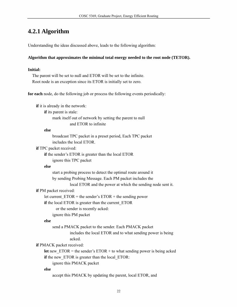
Understanding the ideas discussed above, leads to the following algorithm: Algorithm that approximates the minimal total energy needed to the root node (TETOR). Initial:
The parent will be set to null and ETOR will be set to the infinite. Root node is an exception since its ETOR is initially set to zero.
for each node, do the following job or process the following events periodically: if it is already in the network: if its parent is stale: mark itself out of network by setting the parent to null
and ETOR to infinite else broadcast TPC packet in a preset period, Each TPC packet includes the local ETOR. if TPC packet received: if the sender’s ETOR is greater than the local ETOR ignore this TPC packet else start a probing process to detect the optimal route around it by sending Probing Message. Each PM packet includes the
local ETOR and the power at which the sending node sent it. if PM packet received: let current_ETOR = the sender’s ETOR + the sending power if the local ETOR is greater than the current_ETOR
or the sender is recently acked: ignore this PM packet else send a PMACK packet to the sender. Each PMACK packet
includes the local ETOR and to what sending power is being acked.
if PMACK packet received: let new_ETOR = the sender’s ETOR + to what sending power is being acked if the new_ETOR is greater than the local_ETOR: ignore this PMACK packet else accept this PMACK by updating the parent, local ETOR, and
22

COSC 5369, Graduate Project, Energy Efficient Routing
transmission power The probing processing described in the algorithm is a procedure in which a node increases its transmission power for the PM message gradually while listening for one or more ACK messages; hence the node gets a chance to know the exact transmitting power needed to transmit a data packet to another node.
4.2.2 Proof
We show that the algorithm presented above can approximate the global minimal TETOR (Total Energy to the Root node) by the following two steps:
1) The algorithm is able to take all the reachable nodes into the network eventually.
Proof: Suppose that all the nodes are in two sets: S={ni | ni is a node that is already in the network} F={nj | nj is a node that is not in the network} Since the nodes in S keep broadcasting TPC packet periodically, one node j in F will receive one TPC packet sooner or later, from that point, node j starts probing the neighbors around it. According to our algorithm, it will finally be acked since the ETOR equals to infinite.
2) Every node keeps trying to adjust its parent and transmission power to save more energy
without increasing the cost for other nodes to send data to the root.
Proof: The opportunity for a node to adjust its parent and ETOR occurs only when a PMACK packet is received. It is easy to see that all the bad routing will be ignored, so a node is always trying to get a smaller ETOR value and to choose the parent who can give it the better value. From this algorithm, it is easy to see that when a node gets a better ETOR value, it gets more chances to acknowledge the PM packet sent from other nodes. From the discussion above, a node accepts those ACK packets only if it can get a better ETOR by choosing this node as its parent. Hence, a node getting a better ETOR would not harm other nodes to get better ETOR value.
End of Proof
23

COSC 5369, Graduate Project, Energy Efficient Routing
4.3 Algorithm Analysis
In this section, we will be concerned with the following questions of the algorithm:
1) What is the advantage of the algorithm? 2) Constructing time, that is, how long will the algorithm take to bring N nodes up to the network
from the beginning? 3) Energy cost of probing process 4) Converge time, that is, how much time is needed for the algorithm to converge?
4.3.1 What is the advantage of the algorithm?
The advantage of the algorithm is that it decreases the cost for replacing the dead batteries. We show this by the following discussion. Notice that our target model is a flat-network [1], that is, all the nodes have been assigned the same role; hence all the nodes sample and send the data in the same manner. For one node who has n children, it must do routing for all of its children, hence the total energy consumption for that node is:
E=(n+1) * power_to_its_parent, where n is number of children As the height of the sub tree increases, n increases exponentially. In a short-path based algorithm, nodes in the network tend to select the parent as far as possible, hence the resulting network has a smaller average value of height. In our algorithm, each node tends to use the minimal transmission power, hence more hops are needed for each node, which results in a higher average value of height in the resulting network. It is clear that the inner nodes consume their energy much faster than the outer nodes do in the resulting network because the number of the children increases exponentially as the height of the sub tree increases. That is, the new algorithm saves the costs in replacing the dead batteries by moving the main part of the total energy consumption to the inner nodes. This conclusion is based on a reasonable assumption: the nodes closer to the base station can be more easily maintained.
4.3.2 Constructing time
We can assume that every existing node in the network will broadcast TPC messages periodically, the TPC begins to propagate from the root node along the direction of radius to the edge of the covered area of the deployment. From the statistic point of view, we can think the radius of the network increases gradually by one transmission radius of TPC message at the frequency that TPC messages are broadcasted. If we consider the application being deployed on a surface (our target model), we have:
24

COSC 5369, Graduate Project, Energy Efficient Routing
2** rN πρ= [4.1]
Where ρ is the density of the sensors in the deployment, r is the radius of the current network. Hence:
tfr tpc≥ [4.2]
Where fTPC is the frequency at which the TPC message has been broadcasted periodically, t is the current time from the beginning of the network. So Equation [4.1] can be written:
2)(* tfN tpcπρ≥ [4.3]
2)(*
tfNtpc≥⇒
πρ [4.4]
πρ *Ntftpc ≤⇒ [4.5]
Nff
N
ttpctpc
*1**1*πρ
πρ=≤⇒ [4.6]
For a given application, we can consider ρ constant and fTPC constant, the time needed for constructing the network is within the following computational complexity:
)( Nt Ο= [4.7]
In Equation 4.2, the reason why the radius of the current network may be greater than is that TPC
propagates faster than . This is an implementation issue and will be discussed in subsection 6.3.3 in
Chapter 6.
tf tpc
tf tpc
4.3.3 Cost of probing process
The probing process is to detect the minimal transmission range to a parent. A node starts probing when it receives a TPC message with a better ETOR. The probing process starts with a small starting power (denoted by P0), increases by a constant increment (denoted by Ps), and finally ends with the maximum transmission power (denoted by Pn). It is obvious that probing process is costly in terms of energy. Following the high cost fact, or, a question
25

COSC 5369, Graduate Project, Energy Efficient Routing
is brought up: is it worth it? It is not hard to realize that whether it is worth it or not is actually depends on the particular application request. For example, in an application, there are a lot of data packets sent from all nodes to the root and all nodes in the network are stationary. In this situation, energy used to send data packets takes up most power usage of each mote. Hence finding the minimum transmission is worth doing. Furthermore, after the network has been established, we can slow down the frequency at which the probing process is triggered periodically to save more energy in probing process. Certainly the necessity of slowing down the frequency is application dependent as some applications are critical in topology changing while other applications are not. In this project, focusing on the algorithm itself, changing the frequency for triggering probing process will not be considered and will be set to a constant. Certainly, different parameters for the probing process have the different effects in our algorithm. How these parameters affect the algorithm will be discussed as following:
a) Increment (Ps)
We discuss Ps first since it looks less interesting to us. It is easy to see that a smaller Ps gives a more precise result while consuming more energy because for one probing process the energy needed is:
nss PPPPPPP ++++++= ...)*2()( 000 [4.8]
Formula [3.8] is an arithmetical progression with ⎥⎥
⎤⎢⎢
⎡ −
s
n
PPP 0 terms, hence:
2*
2* 0000 n
s
nn
s
n PPP
PPPPP
PPP
+−≥
+⎥⎥
⎤⎢⎢
⎡ −= [4.9]
s
n
PPP
P 1*2
20
2 −≥⇒ [4.10]
So the smaller Ps is, the more energy is needed to finish one probing process; on the other hand, a smaller Ps results in a more precise detection of transmission power. We will compare the results with the different Ps in simulator. b) Starting Power (P0)
What happened if we start the probing process with a bigger P0? Answering this question is simple but the result is amazing: once nodes try to reach the parents that are far from them, a multi-layered network will be constructed. Especially when P0 equals to Pn we get a case with shortest path. Figure 4.1 shows how and why this can happen.
26

COSC 5369, Graduate Project, Energy Efficient Routing
Figure 4.1
The red line and circles show the minimal transmission range decided by P0, the blue lines show the routes for all nodes. We notice that D goes to B directly (also C to A and B to R) because D will ignore the ACK messages from C since B’s ETOR is less than C’s ETOR The benefits of increasing P0 are obvious:
1) The multi-layered network is considered to be able to save more energy for the inner nodes which are close to the root node, because the inner nodes do not have to route the packet for every one “behind” it.
2) It also decreases the transmission delay time because the number for the relay nodes for one
path has been decreased.
The above discussion suggests that this algorithm allows tradeoff among transmission delay, load of the inner nodes, and total energy savings.
c) Ending Power (Pn)
In considering ending power, we focus mainly on the following two questions: 1) What happened if we use a smaller value? 2) What happened if we have a bigger value?
For a smaller value of ending power, we may end up not being able to bring all the nodes up to the network. On the other hand, a bigger value of ending power allows more precise computation of the optimal routing tree while increasing the probability of packet collision. Besides packet collision in MAC layer, we are more interested in the response when a node receives too many PM packets. Let us discuss it in detail.
27

COSC 5369, Graduate Project, Energy Efficient Routing
With a constrained RAM size, each node can have only a limited buffer size for all outgoing packets. An out going packet has to be dropped if the buffer is full.
In the real world situation, the sensors in network are usually over-densed [23, 24], which
means there are always extra sensors settled down with much smaller range than the range that the transmitter can reach with its maximum transmitting power.
Obviously, the most serious failure scenario we will meet if PM power is not necessarily large is: one node will receive too much PM from distant nodes; hence the received incoming PM will overrun the current node’s buffer. One may think of increasing the buffer size to conquer this problem, but only if you have infinite buffer size, can the buffer overflow problem be solved. For any finite buffer size, if the incoming message rate is always larger than the rate it generates and sends out the Acknowledgement (ACK), the buffer will definitely overflow sooner or later. So we are not concerned about the buffer size for each mote; what is important to us is how to avoid the buffer overflow problem by limiting our maximum PM power using the following assumptions:
Assumption 1: The sensors are equally distributed over the area covered by the sensor network. This is because we can always assume that the finite set of sensor locations is a subset of infinite outcomes of equal distribution.
Assumption 2: In the probing phase, the incoming messages comply with the Poisson distribution. Assumption 2 is reasonable since in most cases the arrival rate is assumed to be Poisson distributed in the query theory of network performance analysis. [32]
Assumption 3: The necessary transmitting power is proportional to the square of the distance the transmitter can reach. (Recall Formula [2.1]) This is obviously a weak assumption that we took no empirical wireless propagation model into consideration. We only choose the simplest way that the power relates to the distance to ease our consideration. Different models can be applied to implement the network, but the results from assumption 3 still stand reasonably.
Assumption 4: The node disposes the message (process and send ACK) at a constant average rate. The node will surely achieve a constant average rate for disposing messages after a certain long period of time.
Now, we assume that node i is the node receiving PM from all the other nodes and sending ACK for
all the PM it received. We denote the maximum PM power by ,A represents the total area covered
by the sensor network, for the total number of nodes within the network,
maxPM
N α for the ratio of
transmitting power to the square of distance it can reach assumed to be a constant by assumption 3;
for the distance between node k and node i,
ikD
inλ for the parameter of the Poisson arrival rate at node i on
28

COSC 5369, Graduate Project, Energy Efficient Routing
which we based our analysis, )(kinλ for the arrival rate of node k to node i, outλ for the average disposing
rate (the same value for each node, it is also the out coming rate for each node), Dρ for the probability
density of existence of a node at distance D.
Since the incoming rate of node i is the sum of incoming rate of node i from all the other nodes, that is:
∑≠=
=N
ikkkinin
,1)(λλ [4.11]
In the equation above, each term )(kinλ is equal to the product of the out coming rate of node k ( outλ )
and the probability that the PM from node k will reach node I, thus:
outachPMkin P λλ ×= Re)( [4.12]
Since we are increasing the PM power at node k from zero to continuously, since the distance
between node I and k is , to reach node I at distance , the minimum transmission power is
according to assumption 3. If we only consider the node in maximal transmission range covered
by PMmax, the probability that the PM from node k will reach node I is ():
maxPM
ikD i
kD
2)( ikDα
max
2max
Re)(
PMDPMP
ik
achPMα−
= [4.13]
Furthermore, we need to calculate the probability that at distance D there exists a node. As stated above, there are N sensors (nodes) equally distributed over area A, so the node density is N/A, we can write the node existing probability at distance D as:
ANDD
DDDD
nodenodenode
DD
ππρπρπρ
ρ 22)( 22
0lim =×=
∆∆−×−×
=→∆
[4.14]
Hence the balanced incoming and out coming rate equation for node i can be achieved here:
29

COSC 5369, Graduate Project, Energy Efficient Routing
dDAND
PMDPMP
out
ik
N
ikkkinin ∫∑ ××⎥
⎦
⎤⎢⎣
⎡ −==
≠=
α λπαλλ
max
0max
2max
,1)(
2)( [4.15]
It can be easily proved that the incoming and out coming ratio at node i complied with the relation:
max0max
2max
22)(max
PMANdD
AND
PMDPMPM i
k
out
in
αππα
λλ α =×⎥
⎦
⎤⎢⎣
⎡ −= ∫ [4.16]
To avoid buffer overrun, the ratio above, which is the averaged ratio over long time period, should be no more than one. That is:
12 max ≤= PM
AN
out
in
απ
λλ
[4.17]
Written in the form of constraint for the maximum PM power:
NAPMπα2
max ≤ [4.18]
It is necessary to point out that the above formulas just give us an idea of the minimum factors will interact with the power of probing messages, in realistic; choosing the power of probing messages is more likely to be an engineering decision.
4.3.4 Converge time
Precise analysis of converge time is not so easy. This is because converge time is affected by at least the factors following: 1) Packet losing of TPC rate: a losing TPC packet delays the time for triggering the other nodes to detect
the neighbors. 2) Packet losing of PM: a losing PM packet makes the sender take at least one more probing process to
get converged. 3) Error in detecting: error in detecting is caused by interaction among the nodes and has the same effect
of packet losing of PM; the following scenario illustrates one instance of the problems caused by interaction among the nodes:
30

COSC 5369, Graduate Project, Energy Efficient Routing
Figure 4.2
In Figure 3.2, the red circle denotes the coverage area for one probing message. Suppose nodes A and B are currently not in the network (that is, both of them don’t know where their parents are) and node R stands for a node that is already in the network, that is, according to our algorithm, node R will ACK the probing message from B to make B to get into the network. The point is that node A is going to be acked by node B; however, node A will be acknowledged at an unnecessary high transmission power, notice that in the Figure 3.2, the coverage area of the PM message from A is not necessarily large enough to cover B. Also node A needs at least one more probing process to be converged. 4) It is even hard to define what being converged means. The working environment keeps changing, which makes link qualities not constant, hence nodes in the network may adjust the topology by chance even if the network exists for a long time. How to define a model in which a topology change can be determined either for constructing the network or for maintaining the network is also not easy. The difficulties for creating a concrete model of either one of factors mentioned above for analyzing make the precise analysis of the algorithm impossible for this project. Precise analysis of the algorithm will be a suggestion for future work. For the present, a simple discussion can help readers get a preview of the answer to convergent time problem. Since the algorithm tends to choose the shortest links from a probability point of view, there is an average distance D covered by the transmission power closing to the minimum probing message, at which the “converged network” expands. So despite many other factors that affect the convergent time, we have:
a) A smaller beginning power for probing message results in a longer converge time b) As the radius of the converged network increases linearly, the coverage area increases squarely,
from computational complexity point of view, convergent time is bounded by )( NΟ if the
nodes are evenly distributed.
31

COSC 5369, Graduate Project, Energy Efficient Routing
Chapter 5: Development In this chapter, we will describe how the development platform has been configured. Discussions will focus on the implementation issues, or the way in which algorithms are implemented. Architecture of the application will be presented. We have also discussed other implemented parts of the project such as why and how the core source codes of ATEMU was modified, and how the visualized log file analyzing tool program was developed.
5.1 Platform of development and Computing Environment
5.1.1 Software and Platform
The following softwares and Platforms are used in this project:
Software Version Operating System Red Hat Linux 9.0 Tiny OS 1.1.0 ncc 1.1.1 (source) gcc 3.2.2 JDK IBM-JDK 1.3 for Linux ATEMU 0.4 (source)
Table 5.1 Note:
1) At the time we installed our system, ncc-1.1.1was not directly available on the website of Tiny OS. The available ncc version 1.1.2 was not compatible with gcc-3.3.2, which is embedded in RH Linux release 9.0. We need to download the source code of ncc-1.1.1 and install it manually. Hence the Tiny OS rpm packet has to be installed by –nodeps option.
2) By the time we installed our system, IBM had changed the name for its JDK 1.4. Using IBM JDK
1.4 may cause problems when installing tiny OS. That’s the reason we used IBM JDK 1.3 eventually.
5.1.2 Tiny OS
Tiny OS is a component based, event oriented operating system for wireless sensor network. The component based model allows rapid application development and small sized code while the event
32

COSC 5369, Graduate Project, Energy Efficient Routing
oriented model saves a lot of energy by allowing the system to enter a sleep mode and to be awaked when something happens [19]. Tiny OS is also designed for more than one hardware platform. Currently, Berkeley/Crossbow Motes is the most commonly used hardware in related researches.
5.1.3 Active Message
Active message model is the most important part in Tiny OS for radio communication. Each packet in Active Message model is short and has fixed length, attached with a type id and a group id. When an Active Message packet is received, the Tiny OS looks at the header of the received packet. If the group id is matched with the current application, it continues to check if there is an event handler attached with the type id. If there is a related event handler, Tiny OS fires the event for that handler, from which the application takes control of the system. Active Message model allows different applications to run concurrently in one network by giving each application a group id. Furthermore active message model allows different applications to run concurrently in one sensor by assigning each type of packet a different event handler. The Tiny OS-1.1 release and its later versions include library components that provide ad-hoc multi-hop routing for sensor network applications. Although these components have been designed for other route-decision schemes, the components come with the Tiny OS are only implemented with the shortest path algorithm. As well known, shortest path route-decision scheme is usually not a good choice in a wireless network. For energy efficiently data collection, there is certainly a lot of work to be done in Tiny OS. [19, 33]
5.1.4 TinyDB
TinyDB is another important application for Tiny OS. TinyDB simplifies the data collection tasks in most cases. We consider that not only what we did can be used in a particular application, but also to improve the design and implementation issues in Tiny OS and sensor networks. [19, 34, 35]
5.2 Implementation Issues
When implementing our algorithm, we must consider the following issues: 1) What is the memory constraint of our program? 2) How large should the power be for probing messages? 3) What is the power need for the TPC message? 4) Do we need to handle the case of packet loss?
33

COSC 5369, Graduate Project, Energy Efficient Routing
5) Is dynamic memory management needed? 6) AM message or low level communication?
Keeping in mind that our project is a research-oriented project in mind, we will discuss what the considerations and choices for each implementation issue we made.
5.2.1 Memory constraints
On the hand since our program is going to be used as a component for other programs, we should use as little memory as we can; on the other hand, our program has to queue all the out going packets, because the radio component has to be accessed exclusively, otherwise, packet loss will result. Table 5.2 shows the memory usage of some typical Tiny OS applications:
Application Memory Usage (byte) TinyDB Less than 3100 Moté 849
Table 5.2 Usage of Typed Tiny OS applications [34, 44]
We will limit the RAM usage to about 1K bytes. This memory is used mainly for the buffer size of the out-going messages, and hence can be adjusted to make a tradeoff between memory size and other memory demand in a real application.
5.2.2 Probing message power
According to the discussion in Chapter 4, we compare the advantages and the disadvantages for the different probing power in the following table:
Starting power Increment Ending power Smaller Bigger Smaller Bigger Smaller Bigger
Precision √ √ √ Converge Time √ * * * * Energy Consumption √ * * * *
Table 5.3 Comparison of different power probing strategy Note: ‘*’ means no obvious relationship according to the discussion of Chapter 3
Because the density of the network is determined by how the node is deployed and can be controlled by the transmission power [41], so at the beginning we just set those values as following:
34

COSC 5369, Graduate Project, Energy Efficient Routing
Starting power: 1 Step: 10 Ending Power 150
These settings give us flexibility to decrease or increase them in later implementation because the maximal transmission power is 255. We will compare the effects when using different values of those powers in testing.
5.2.3 TPC Power and Period
According to our algorithm, a node sets up a probing process after receiving a TPC packet. When the probing process is not yet finished yet, it is not necessary to broadcast another TPC packet. On the other hand, the speed of a simulation process in ATEMU is much slower than the real world application does. Therefore the TPC packets are supposed to be sent in frequencies as high as possible in order to speed the simulation process. It has been shown in Section 4.2.2, that a probing process may take (150-1)/10 ≈ 15 circles to finish. Furthermore, the random delay circles will be apply to make the probing message reach-rate more evenly distributed, before a node starting its probing. This random delay circle will be set to 0-10 and will be discussed later in the program. From the above discussion, 30 system time circles are selected for a node that is in the network to broadcast the TPC packets. This is because 30 is larger than the sum of 15 and 10, that is 30 > 15+10. It is obvious that the power of TPC should be the same amount as the maximum power of probing messages. Otherwise, it will waste energy because some nodes will be triggered to probe but will not be able to reach the sender.
5.2.4 Packet loss
Packet loss may result from two sources: 1) packet collision in radio communication media, 2) packet dropping in motes. The first case is well studied and sometimes called “exposed node problem” [45]. The second case is because the radio component has to be accessed exclusively [20]. If a packet is in sending, the program has to wait until the sending process is finished to send the next packet, which means the program has to put the packet to be sent into an outgoing buffer. When the buffer is full, the program can do nothing but drop the packet. It is better to prevent packet loss than to solve it. Packet loss can be avoided by holding a big buffer. However, a packet has to be dropped occasionally because of the constraint on RAM usage that exists in
35

COSC 5369, Graduate Project, Energy Efficient Routing
reality. The TPC message plays an important role in constructing and maintaining the network. PM and PMACK are used to probe the exact power needed to transmit to a particular neighbor. The loss of these packets delays the convergent time of the entire network, so, it is tolerable to lose some of them although they carry different functionalities. The conclusion is made because there is no general way to solve the side effects caused by losing of packets. In practice, the buffer size is usually adjusted so as to minimize the potential packet loss. To increase the speed of simulation of the entire network via a designing approach, one node may receive too many messages in a relatively short period of time. Under all these considerations, a buffer size of 16 is selected.
5.2.5 Dynamic memory management
Since a big buffer is preferred, it may be asked that whether it is necessary to implement a dynamic memory management, so that our program can use as much memory as the system can support.
The code for dynamic memory management introduces more CPU load. To meet the memory constraint, an embedded computing system usually must use a constant memory to improve its performance.
In a real world application, the network traffic will not be as heavy as it is in our testing environment.
It is safe to conclude that it is unnecessary to apply dynamic memory management.
5.2.6 AM message or low level communication
As being discussed in the introduction of the report, data collection is much more than just sending data back to the root node. For example, the data may be aggregated within a small group of sensors that are geographically close to each other before they are sent back to the root node [10], thus the application may have more than one preferred path for the packets. To examine such possibilities, the following approaches have been adopted in designing the program: using one channel of AM message instead of controlling the byte or low level communication. Using AM message not only simplifies implementation but also makes it possible to move the existing programs to our frame work easily, because the only things these programs need to do to take advantage of our component are querying the parent node and the transmission power to the parent node. Figure 5.1 shows the architecture of the component with an imaginary application from the view point of communication.
36

COSC 5369, Graduate Project, Energy Efficient Routing
Customer Program
EnergyEfficientRouting Layer
Figure 5.1 System structure of the implementation
As shown in Figure 4.1, EnergyEfficientRouting represents the main part this project. Our program uses AM Message and controls the hardware directly to discover the most energy efficient route. A bidirectional arrow indicates that not only the upper layer program call commands of the lower level program, but also the upper layer program is responsible for handling events from the low level program. A directional arrow starts the upper layer program calls commands of the low level program. It is clear that a customer program queries only the necessary information for energy efficient routing and is free to use an AM message directly as it usually does. A typical scenario is that when an application needs to send data back to root node, it calls the program to get the information about which link and how much power is needed for that link, and then sends the data packet with the information from our program through AM message. One obvious advantage of this architecture is that it allows more than one routing schema to exist in the whole application, so that the customer program is not forced to use our component only.
5.3 Main Program
Our main program is a Tiny OS component called EnergyEfficiencyRoutingC written in NesC language. We discuss how it has been implemented by introducing the configuration of our application.
5.3.1 Configuration an imaginary application
The configuration we will discuss in this section is decided by the Tiny OS programming model. A configuration describes how the different components of the whole application cooperate together with one another. As shown in Figure 5.2, the components in yellow are our programs.
AM Messages CC1000Control
37

COSC 5369, Graduate Project, Energy Efficient Routing
Figure 5.2 Components hierarchy
In the above diagram, components LoggerC, UARTM, LedsC are only used for debugging and can be removed for a real application. An arrow in the diagram indicates one or more relationships between the connected parts. The detailed configuration diagram can be found in Appendix D.
5.3.2 Core component details
The core component of our program includes an interface, a configuration and a module (interface, configuration, module are in terms of NesC language [43]). A separate C language header file is used to store the parameters of our algorithm. Interface: IEnergyEfficiencyRouting We have made our API (Application Programming Interface) as simple as we can. Only two commands are needed as described as table 5.4: Command Purpose getParent Get the parent node. A TOS_BCAST_ADDR means the parent node is currently
unavailable. getPower Get the transmission power to the parent.
Table 5.4 Configuration: EnergyEfficiencyRoutingC
EnergyEfficiencyRoutingC
LoggerC
SimpleApp
CC1000Control GenericCo TimerC LedsC
Other Tiny OS Components Needed by SimpleApp UARTM
38

COSC 5369, Graduate Project, Energy Efficient Routing
Configuration EnergyEfficiencyRoutingC is used to wire our core module with the necessary components. ‘Wire’ is a term of NesC language for connecting different components together. Module: EnergyEfficiencyRoutingM Module EnergyEfficiencyRoutingM is the core part of the programming in which the algorithm has been implemented.
5.3.3 Queued outgoing message
Because of the memory constraint in sensors, a Tiny OS application has to handle the message buffer by itself. A typical Active Message usage is as following. The application calls the function of Tiny OS radio communication component with a message buffer to start sending process. Then the application will be notified if the sending process is finished, with the buffer returned to the application. During the whole process, the buffer cannot be used for other purposes. So there is a problem such is: There is more than one message to be sent while the current sending is not yet finished. Our approach to solve this problem is to have an outgoing message queue. Any outgoing message will be appended to the queue and a task will be used to send the outgoing messages whenever the queue is not empty and the last transmission is finished. Because a task can be interrupted by an event, the exclusive access to the queue must be protected by an atomic section [43].
5.3.4 Timer
Our program is time-driven structure, that is, most periodic tasks such as broadcasting TPC packets will be put into a timer event that is fired at a constant rate periodically. The reason we implemented our algorithm in this way is that we can easily use the number of ticks a sensor has to take to reach a state, which is more precise than using a real timer to measure the time complexity of the algorithm. Since we are going to test our algorithm in simulator, the simulating speed is heavily affected by how many nodes there are in simulation. In later discussion and analysis in Chapter 5, we will use time tick system or system time to refer to the idea introduced above.
5.4 Test application construction
Certainly there are many different applications for sensor networks. Each one of them has its own node distribution model, so it is impossible for us to test our program in so many applications. For our test configuration, we used a program described as follows to generate our test configuration: our program will take the given width and height parameters and generate a rectangular area, then put a node randomly
39

COSC 5369, Graduate Project, Energy Efficient Routing
in each grid with both width and height equal to 50 meters. Figure 5.3 is the main configuration of the testing phase. Here, the configuration is a given application with deterministic geographical sensor locations.
Figure 5.3 Configuration with determined geographical sensor locations
Generated by eegraph The node with id zero is the root node.
5.5 Debugging
Because ATEMU simulates the Tiny OS application at the hardware level, there is no console (console here means a tradition text based terminal between human being and machines) which other simulators have. ATEMU itself is able to log every low level event such as I/O operations, function calls, etc. However, the assembler level debugging information is not so helpful in debugging our application. What is desired is the ability to print messages in console (or log file) so that we can easily trace all the high level actions of the application. We have contacted the authors of the ATEMU and some experts who have been using ATEMU. All suggestions lead us to the idea of intercepting the byte stream for a UART, Universal Asynchronous Receiver/Transmitter, a hardware component that controls serial device communication. Since we prefer printing messages to recording a low level byte stream, we designed our debug/log part as described in Figure 5.4
40
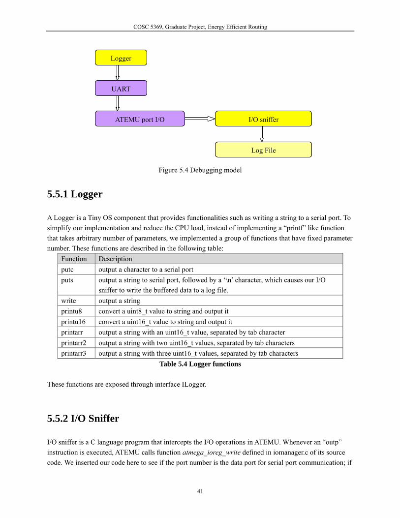
COSC 5369, Graduate Project, Energy Efficient Routing
Logger
UART
ATEMU port I/O I/O sniffer
Log File
Figure 5.4 Debugging model
5.5.1 Logger
A Logger is a Tiny OS component that provides functionalities such as writing a string to a serial port. To simplify our implementation and reduce the CPU load, instead of implementing a “printf” like function that takes arbitrary number of parameters, we implemented a group of functions that have fixed parameter number. These functions are described in the following table:
Function Description putc output a character to a serial port puts output a string to serial port, followed by a ‘\n’ character, which causes our I/O
sniffer to write the buffered data to a log file. write output a string printu8 convert a uint8_t value to string and output it printu16 convert a uint16_t value to string and output it printarr output a string with an uint16_t value, separated by tab character printarr2 output a string with two uint16_t values, separated by tab characters printarr3 output a string with three uint16_t values, separated by tab characters
Table 5.4 Logger functions
These functions are exposed through interface ILogger.
5.5.2 I/O Sniffer
I/O sniffer is a C language program that intercepts the I/O operations in ATEMU. Whenever an “outp” instruction is executed, ATEMU calls function atmega_ioreg_write defined in iomanager.c of its source code. We inserted our code here to see if the port number is the data port for serial port communication; if
41

COSC 5369, Graduate Project, Energy Efficient Routing
the condition is satisfied, our code puts the outgoing character to a buffer array. Whenever a buffer is full or a new line character is received, the program flushes the content of that buffer to a log file. The size of buffer array is adjustable and set to 1000 in our program, which allows our log system to log the first 1000 nodes in a test application.
5.5.3 Log File
Our log file is a plain text file. Each line in a log file can be viewed as an application layer event such as a packet sent, a parent found, etc. Each line consists of two parts: node id and event description. For the first few lines in a log file, root node (the node with id zero) will print the chosen parameters for the corresponding test. Each packet sent is identified by a packet type in parenthesis. The system timer printed by root node consists of two numbers: the high 16 bits and the low 16 bits of a 32 bits timer counter. A log file contains enough information to trace all the actions taken by the program. The following lines of output are an example of a log file content:
000 -- system timer: 0 4 000 <pmack> to 7 006 <pmack> to 1 007 parent ETOR power 0 21 21 001 parent ETOR power 6 32 21 006 <pmack> to 7 007 drop pmack from 6 008 <pm> 31 007 <pm> 31
It is easy to know what happened among nodes 0, 6, 7 in system timer numbered 4: node 0 sends a pmack packet to node 7, and this causes node 7 accepts node 0 to be its parent (the fourth line). Node 6 sends a pmack packet to node 7 also indicated in the third line; but node 7 refuses to accept node 6 as its parent node since node 7 already has a better route (line 7).
5.6 Methods of Log File Analysis
The log file can be easily analyzed by many text tools which come with the Linux system. We will introduce methods been used for each particular analyzing task.
42

COSC 5369, Graduate Project, Energy Efficient Routing
5.6.1 View interactions of one node with other nodes
In debugging phase, there is a common case in which we want to know what happened between a particular node and the other nodes. The following bash command with sample node 7 is used for this purpose:
grep –E ‘(^007)|(pmack.*7$)|(system)’ ee.log The filename ee.log is the default filename generated by our log system.
5.6.2 View the history of one node for changing the parent node
As we described in early chapters, our algorithm will converge gradually. Knowing how a node has changed its parent node is helpful in analyzing our program. The followed bash command is an sample command for node 7:
grep ^007 ee.log | grep parent
5.6.3 View the final topology of the network
Each node may change its parent node as the time passed; the last change is one part of the final topology of the network. The bash program final_topology shows what the topology is:
#!/bin/bash for i in `cut -b1-3 $1 | sort -u` do grep ^$i $1 | grep parent | tail -n 1 done
5.6.4 Visualize the log file by eegraph
We also have developed a visual tool called “eegraph”. It reads the positions of network configurations and a log file, interprets the log file and draws the graphic according to what was happening in the network as recorded in log file. We will discuss eegraph in more detail about in Chapter 5.
43

COSC 5369, Graduate Project, Energy Efficient Routing
5.7 Assign ID for each node automatically
Usually, a simulator assigns a different ID for each node automatically when the corresponding binary image is loaded. This is done by substituting the value of a constant variable named with TOS_LOCAL_ADDRESS. In ATEMU, since it allows different applications to run together, instead of assigning ID automatically, it allows the developer to assign an ID for an each node. However, this amazing function sounds like a bug to us. Because there is no official support from ATEMU’s development team, we devised a different method to assign different IDs for each node automatically. Our approach involves three steps:
1) Modify the source code of Tiny OS to allow it to accept a macro definition of NODE_ID. The Tiny OS file involved is $TOSDIR/system/tos.h. This file will be submitted by the project cdrom.
2) Modify the default Makefile to take an environmental variable as the definition of NODE_ID. 3) Write a bash script to assign the environmental variable to a value and call make tool iteratively.
44

COSC 5369, Graduate Project, Energy Efficient Routing
Chapter 6: Testing and Analyzing In this chapter, programs are tested in the simulator - ATEMU with different parameters and different configurations; Different results are compared to obtain better understanding of the algorithm. Since the maximal transmission power is an alternative view of the density of the nodes [41], so 150 units has been chosen as the maximal transmission for all configurations. Effects of the different parameters of probing messages are analyzed. In this chapter, the methodology that is used to analyze the log file will be introduced, and results will be studied.
6.1 Methodology
6.1.1 Simulator
Simulator “ATEMU” [36] is used to verify and analyze the algorithm. When choose simulators, there are mainly four kinds of simulator listed below followed by a short illustration for each of them.
1) TOSSIM: It comes up with Tiny OS package. Tiny OS provides a visualization tool called TinyViz to cooperate with TOSSIM. TOSSIM is able to simulate most applications based on Tiny OS, however, it does not simulate the program on a hardware level. Since we may need to adjust the transmission power dynamically, we did not selected TOSSIM because it is no good for such a low level simulation. More information can be found in [37]
2) ns2: ns2 is a well known network simulator. Although it was originally designed for internet
research, more components have been added to allow it to be a candidate for sensor network. Both ns2 and TOSSIM simulate the sensor network in a packet level, hence not good enough for our project. [38]
3) ATEMU: At the time we needed to decide which simulator to used, ATEMU from University of
Maryland was the only simulator that claims to give the highest fidelity simulating result by simulating the application at a machine code level. [36]. The bad news is that ATEMU is no longer in active development, so there are few resources about it on internet and if we decide to use it, we are pretty much on our own. In our project, we used ATEMU and we have successfully handled the shortcomings of ATEMU.
4) Avrora: Avrora is a new simulator for sensor networks. An advanced algorithm was applied to
make it much faster than ATEMU. We did not choose it, because it does not cooperate with IBM Java development toolkit (JDK), which is the only JDK supported by JAVA SDK in the current version of Tiny OS on Linux system. In windows-cygwin environment, Tiny OS does support Sun JAVA SDK. But we want to put all of our work in a Linux environment not only because it is
45

COSC 5369, Graduate Project, Energy Efficient Routing
stable, but also there are many tools for log file analysis. [39, 40]
6.1.2 Visual Tool
Despite the number of existing text tools in Linux system, we wrote a graphic tool for visualizing the log file in Visual Basic. This visualized tool generates the animation of topology changes in the log file, as well as the total energy needed and total energy consumption for each time period into a csv (Comma Separated Value File Format) file, which can be viewed with Microsoft Excel for graphical analyzing. Basically, program will read the log file as a text stream, parse each line to get the context meaning for that line, draw the corresponding graphical for it, and modify the inner data if necessary. For each 10 system time ticks, program computes the total energy needed and the total energy consumption; the program then outputs that information with the time stamp to a csv file. Figure 6.1 is the screen shot for our program:
Figure 6.1, eegraph screenshot
The red circles stand for the related probing messages and the blue lines stand for parent-children links. To simplify implementation, no arrow will be drawn for parent-children links, since they can be recognized intuitively. Another thing to be mentioned here is that the circle for probing message does not represent the actual coverage of a probing message. This is because we cannot determine the additional empirical radio propagation model applied to the configuration by ATEMU. However, it is still reasonable for us to understand that the geographical location does dominate the radio propagation model in most cases. Not all the possible values for probing messages are tested. Instead, powers of probing messages are changed for several values until we get an idea, about how the different powers of probing messages affect the behavior of the routing algorithm. It is not necessary to wait for the algorithm to reach a
46

COSC 5369, Graduate Project, Energy Efficient Routing
converged state. Instead, each time simulation is terminated when it looks converged: a simulation will be terminated if either of the following conditions is satisfied. First, the whole network does not change for a long period of continued system time; this period must be long enough to cover a TPC period. Second, we already have the information that we want, hence it is not necessary to continue simulation. Our analysis mainly focuses on the following metrics:
1) The final topology, a tree view of the resulting network. 2) Total ETOR, the sum of the ETOR for each node. 3) Construction time, the time needed to establish the network. 4) Total energy consumption, from the beginning to the moment concerned, how much energy has been consumed for the algorithm computing.
In the following sections, we will present the analyzed result for different parameters used in the algorithm.
6.2 Starting power of probing messages
We have explored the following metrics that may be but not necessarily are affected by the starting power: the final topology, total ETOR, the time needed for constructing the whole network, total energy consumption.
6.2.1 Final topology
Figures 6.2 to 6.4 shows the resulting topologies of a configuration with 30 nodes for different starting power of probing messages:
Figure 6.2 Final topology, starting power = 1, generated by eegraph
47

COSC 5369, Graduate Project, Energy Efficient Routing
Figure 6.3 Final topology, starting power = 20, generated by eegraph
Figure 6.4 Final topology, starting power = 40, generated by eegraph
The first thing interesting to us is that different parent nodes for node 14 and node 2 have different starting powers. With starting power equal to 1, node 14 chose node 2 as its parent; while with a greater starting power, node 14 chose the root node as its parent node directly. To verify this, the designed toolkit program is used to dispose each log file and filter out the information about node 14, node 2 and node 6 by the following command:
final_topology 6-5-001,150.log | grep -E '(^014)|(^002)|(^006)' For starting power = 1:
002 parent ETOR power 6 42 11 006 parent ETOR power 0 31 31 014 parent ETOR power 2 63 21
For starting power = 20:
48

COSC 5369, Graduate Project, Energy Efficient Routing
002 parent ETOR power 6 50 20 006 parent ETOR power 0 30 30 014 parent ETOR power 0 60 60
For starting power = 40:
002 parent ETOR power 0 80 80 006 parent ETOR power 0 40 40 014 parent ETOR power 0 60 60
First, we need to describe the format for the listed log file as table 6.1: Column Simple Purpose 1 002 Node id of the node that logged this message. 2 parent ETOR power Indicating the current line is a log message for changing
parent node. 3 0 The new parent node 4 80 The new ETOR 5 80 The transmission power for sending message to the new
parent node. Table 6.1
It is obvious that with a smaller starting probing message, node 2 and node 6 probe the power which is needed to reach the root node more precisely, so node 14 chose node 2 as its parent for starting power equal to 1. As the ETOR for node 2 increases according to the increasing of the starting power, node 14 prefer to reach the root node directly. The same situation happened on node 2, when the starting power increases from 20 to 40. Another point to be noticed is what happened among node 15, 13, 17. The final topology information of these nodes for each case is: For starting power = 1:
013 parent ETOR power 17 73 11 015 parent ETOR power 13 84 11 017 parent ETOR power 3 62 21
For starting power = 20:
013 parent ETOR power 17 80 20 015 parent ETOR power 17 80 20 017 parent ETOR power 3 60 20
For starting power = 40:
013 parent ETOR power 17 130 40
49

COSC 5369, Graduate Project, Energy Efficient Routing
015 parent ETOR power 17 130 40 017 parent ETOR power 0 90 90
If we pay more attention to the transmission power of node 15, the minimal starting power dominates the choice of parent. Although ETOR for node 13 increases by only 80-73=7 points for changing starting power from 1 to 20, node 15 prefers node 17 to be directly connected because the minimal transmission range increases to allow node 17 can be directly detected. Thus node 17 is always preferred since it always has a lower ETOR compared with node 13. This is also an example of how multi-layer network has been formed.
6.2.2 Total ETOR
Figure 6.5 shows the changes of total ETOR value corresponding to the system time tick:
Figure 6.5 Total ETOR for different starting powers, ‘s’ stands for starting power
Generated by Microsoft Chart
At the first 200 system time, the total ETOR increases because more and more nodes are added to the network. Although the curves show that the system has not fully converged, we can easily realize that a higher starting power for probing messages will result in a waste of system power.
50

COSC 5369, Graduate Project, Energy Efficient Routing
6.2.3 Construction time
Figure 6.6 shows the number of the nodes in network according to the system time:
Figure 6.6 Number of nodes in network for different starting powers, ‘s’ stands for starting power
Generated by Microsoft Chart
While ignoring the trivial differences among the curves at a certain time, Figure 5.6 shows that the converging time is not dominated by the starting power. It is reasonable to get such a conclusion because the curves intersect, which means they are growing at a same intrinsic rate. Figure 5.6 also shows that curves with a higher starting power increase faster in most time point, this is because for each probing process, a bigger starting power brings more nodes into network at early time.
6.2.4 Total energy consumption
Figure 6.7 shows the total energy consumption according to the system time:
51

COSC 5369, Graduate Project, Energy Efficient Routing
Figure 6.7 Total energy consumption for different starting powers; ‘s’ stands for starting power
Generated by Microsoft Chart Despite slope of the curve for starting power with 150 units, it is hard to tell what the relationship between total consumed energy and the starting power is. We believe this is because for some relatively small starting powers, the energy saved with a bigger starting power does not dominate the total energy consumption. However, we put the curve for starting power at 150 on purpose to show that if the starting power is big enough, the algorithm can save a lot of energy in probing messages.
6.2.5 Conclusion
We summarize the discussed results as Table 6.1: Metric Relationship with starting power of probing message Final topology A higher starting power results in multi-layered network, the
number of hops for each route decreases Total ETOR A higher starting power results in a higher total ETOR resulted Constructing time N/A Total energy consumption A higher starting power results in less total energy consumption
Table 6.1
6.3 Increment of probing power
The following metrics, which may be affected by the increment of probing power, have been explored:
52

COSC 5369, Graduate Project, Energy Efficient Routing
the final topology, total ETOR, the time needed for constructing the whole network, total energy consumption.
6.3.1 Final topology
Figures 6.8-6.11 shows the final topologies for increment of probing power with 10, 20, 40, 60.
Figure 6.8 Final topology, increment=10, generated by eegraph
Figure 6.9 Final topology, increment = 20, generated by eegraph
53
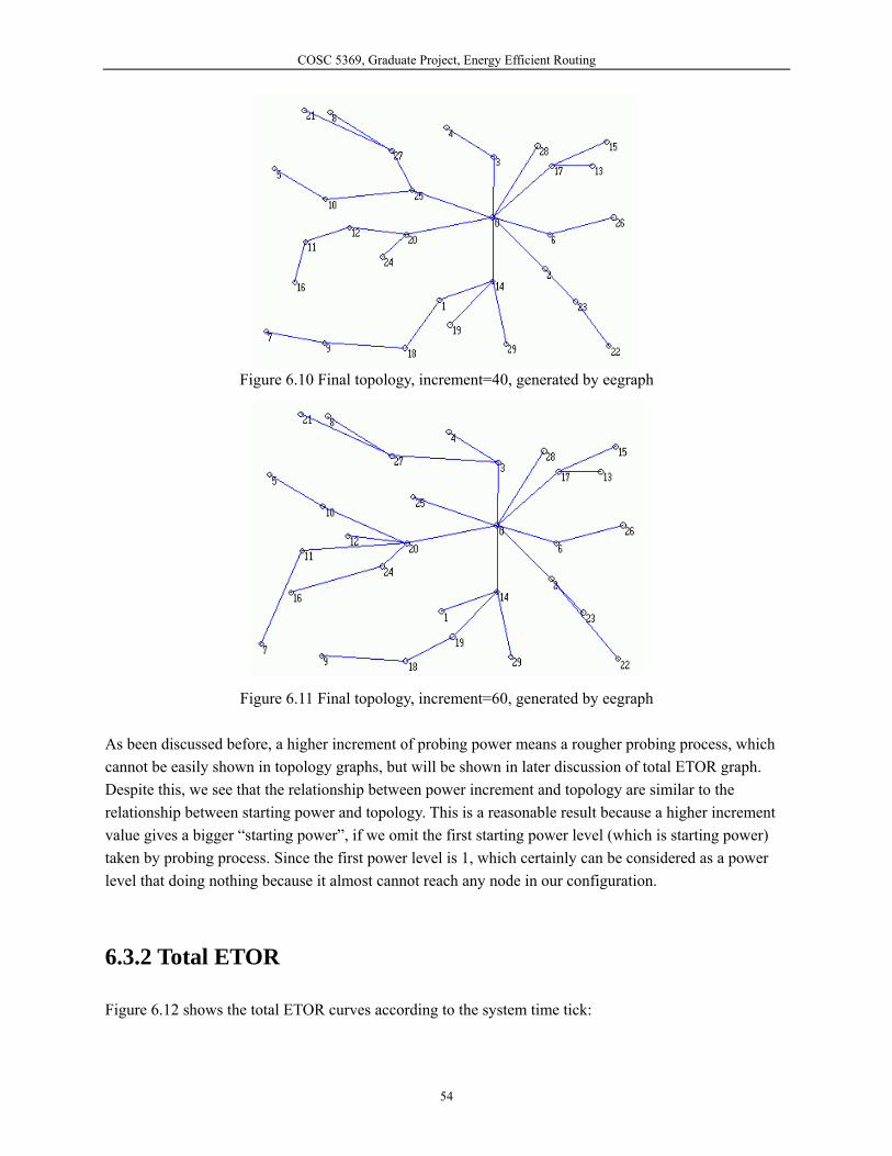
COSC 5369, Graduate Project, Energy Efficient Routing
Figure 6.10 Final topology, increment=40, generated by eegraph
Figure 6.11 Final topology, increment=60, generated by eegraph As been discussed before, a higher increment of probing power means a rougher probing process, which cannot be easily shown in topology graphs, but will be shown in later discussion of total ETOR graph. Despite this, we see that the relationship between power increment and topology are similar to the relationship between starting power and topology. This is a reasonable result because a higher increment value gives a bigger “starting power”, if we omit the first starting power level (which is starting power) taken by probing process. Since the first power level is 1, which certainly can be considered as a power level that doing nothing because it almost cannot reach any node in our configuration.
6.3.2 Total ETOR
Figure 6.12 shows the total ETOR curves according to the system time tick:
54

COSC 5369, Graduate Project, Energy Efficient Routing
Figure 6.12 Total ETOR for different increment, ‘i’ stands for increment
Generated by Microsoft Chart As can be predicated, with a bigger increment for probing messages, the resulted network will consume more energy to transmit data.
6.3.3 Construction time
Although it is predicable that construction time is obviously dominated by the TPC period, notice that from our simulation result, the constructing time for the network is also affected by the incremental value of the probing messages as shown in Figure 6.13:
Figure 6.13 Number of nodes in network for different increments; ‘i’ stands for increment
55

COSC 5369, Graduate Project, Energy Efficient Routing
Generated by Microsoft Chart Because with a random delayed probing process and the different incremental value of probing messages, every network cannot be formed in exactly the same process, a fact to be noticed is that with a bigger incremental value of probing messages, the whole network can be established more quickly. The reason for this is that, with a lower incremental value of probing messages, nodes far away from triggering node need more time to reach the triggering node by increasing probing message power at a smaller constant increment value.
6.3.4 Total energy consumption
Figure 6.14 shows the total energy consumption according to the system time:
Figure6.14 Total energy consumption for different increment; ‘i’ stands for increment Generated by Microsoft Chart
It can be show that as the power increment of probing messages increases, the total power consumed by the algorithm decreases. This is because a bigger increment power of probing message reduces the number of probing messages for each probing process linearly. Although we don’t know the exact reason for that, the curve for increment power equal to 40 units is very close to the curve for increment power equal to 60. We believe this is a configuration related issue since from the previous section of constructing time, the curve for i=40 is also very close to i=60. Future work needs to be done to find the answer.
56

COSC 5369, Graduate Project, Energy Efficient Routing
6.3.5 Conclusion
We conclude the discussed results as Table 6.2: Metric Relationship with bigger incremental power Final topology Multi-layered, the number of hops decreases Total ETOR Bigger total ETOR resulted Constructing time Faster Total energy consumption Less
Table 6.2
6.4 Ending power
Ending power was not tested since a small ending power makes the algorithm more likely to be a greedy algorithm, hence we should always choose a big ending power as long as the packet collision is accepted by the whole application, as discussed in Chapter 4
6.5 Fixed probing power
With a fixed probing power, our algorithm works like a shortest path algorithm. However, the strategy for choosing a parent with a smaller ETOR is still working. We have explored the following metrics that maybe but not necessarily are affected by different fixed probing powers: the final topology, total ETOR, the time needed to construct the whole network and the total energy consumption.
6.5.1 Final topology
Figure 6.15 to 6.18 shows the final topology with the different fixed probing power without an initialized configuration:
57

COSC 5369, Graduate Project, Energy Efficient Routing
Figure 6.15 Final topology, fix=44, generated by eegraph
Figure 6.16 Final topology, fix=66, generated by eegraph
Figure 6.17 Final topology, fix=100, generated by eegraph
58

COSC 5369, Graduate Project, Energy Efficient Routing
Figure 6.18 Final topology, fix=150, generated by eegraph
With a smaller fixed probing power, some distances to the nodes can not be spanned, which is especially bad, as shown in Figure 6.15: node 9 has to go through many parents to reach the root. Fortunately, this is not the usual case since most applications are over-densed, which means the fixed probing power is always high enough to reach more than one node.
6.5.2 Total ETOR
Figure 6.19 shows the total ETOR according to the system time:
Figure 6.19 Total ETOR for the different fixed probing power; ‘f’ stands for fixed
Generated by Microsoft Chart
59

COSC 5369, Graduate Project, Energy Efficient Routing
It shows that there is no obvious relationship between the total ETOR and the fixed probing power. We believe this is because with a small probing power, the algorithm only discovers the shortest links, which tends to save more energy. On the other hand, a big probing power allows the algorithm to make choices among more reachable parents; hence there is also a possibility to save more power.
6.5.3 Construction time
Figure 6.20 shows the constructing time for the different fixed probing power:
Figure 6.20 Construction time for different fixed probing power, ‘f’ stands for fixed Generated by Microsoft Chart
It is can be shown that a bigger fixed probing power results in a faster constructing time. This is because the radius of the network increases linearly as the probing power increases, if the network is over-densed. However, this is not true when the network is not over-densed, which have been shown by the curves for f=44 and f=66. (Recall the transmission range is transmission power is an alterative view of the density of the nodes [41])
6.5.4 Total energy consumption
Figure 6.21 shows the total energy consumption with the different fixed probing power.
60

COSC 5369, Graduate Project, Energy Efficient Routing
Figure 6.21 Total energy consumption for different fixed probing power; ‘f’ stands for fixed Generated by Microsoft Chart
It is obvious that the algorithm consumes more energy with a high fixed probing power.
6.5.5 Conclusion
We conclude the discussed results as Table 6.3: Metric Relationship with bigger fixed probing power Final topology Multi-layered, the number of hops decreases Total ETOR N/A Constructing time Fast Total energy consumption More
Table 6.3
61

COSC 5369, Graduate Project, Energy Efficient Routing
Chapter 7: Conclusions and Suggestions for Future Work In this chapter, the conclusion of this project is given and improvements that can be done in future.
7.1 Conclusion
All the test results indicate that this algorithm is able to approximate a global minimal total ETOR value and save energy in a target network model. More conclusions are made as follows: 1) This algorithm is quite applicable in an over-densed network. An over-densed network gives each
node more choices for the parent nodes and increases the probability that each node can find a best optimal path.
2) This algorithm can behave like a shortest path algorithm by given the different parameters to meet the transmission delay metric for a particular application.
3) The algorithm saves more energy while introduces more transmission delay than the shortest path algorithm does in the target network model.
7.2 Future works
Future works include: 1) As we discussed in Chapter 3, the target network model of this algorithm is a flat-network. One
possible future topic is to find how to use this algorithm in a hierarchical network model. From what can be seen, in the hierarchical network model, it is necessary to aggregate sensors by both the minimal energy needed and geographical information. One solution for this is to allow more than one node in the network have a zero ETOR value and a limited operating range for this value so that each group leader can direct the data packets from its neighbors to itself for aggregation purposes.
2) Allow the TPC period to be adjustable dynamically according to the network situation. This is
necessary to construct the whole network in a short time and improve power usage efficiency. At the beginning of the network operation, this algorithm can use a small TPC period. Once the network is ready for use, the customer program decreases the cost for maintaining the network by slowing down the frequency at which the TPC is broadcasted.
3) An efficient way to determine if the network is converged such that we can slow down the period for
TPC broadcasting. Because of environmental changes and other factors, a sensor network can never be in a static state. So the key to energy savings is to determine if the network constructing phase is finished or not by slowing down the TPC broadcasting period, as discussed in the second future work. From what can be seen so far, an adaptive algorithm can be used for monitoring the topology change.
62

COSC 5369, Graduate Project, Energy Efficient Routing
For a node, if the parent node and the local ETOR does not change for a long time, which means the network around that node is converged, that node slows down its TPC broadcasting period, resulting in more energy saving.
4) More accurate analysis of the algorithm behaviors for real applications. The algorithm was only tested
in the simulator ATEMU. ATEMU is used for high fidelity simulation [36], but, more accurate test data can be obtained only from the real world application test. Testing and studying the behaviors of the algorithm in a real world application is a valuable future task.
63

COSC 5369, Graduate Project, Energy Efficient Routing
Bibliography 1. J. N. Al-Karaki, A. E. Kamal. ”Routing Techniques in Wireless Sensor Networks: A Survey”, IEEE
Personal Communications, Volume 11, Issue 6, pp 6-28, Dec 2004
2. R. Szewczyk, J. Polastre, A. Mainwaring, and D. Culler, “Lessons From A Sensor Network Expedition”, Proc. of EWSN, 2004
3. N. Xu, “A Survey of Sensor Network Applications”, IEEE Communications Magazine, 40(8):102114, August 2002
4. L. Krishnamurthy, R. Adler, P. Buonadonna, J. Chhabra, M. Flanigan, N. Kushalnagar, L. Nachman, M. Yarvis, “Design and Deployment of Industrial Sensor Networks: Experiences from a Semiconductor Plant and the North Sea”, Proc. of EWSN, 2004
5. C. Rahul, J. Rabaey, “Energy Aware Routing for Low Energy Ad Hoc Sensor Networks", IEEE Wireless Communications and Networking Conference (WCNC), vol.1, March 17-21, 2002, Orlando, FL, pp. 350-355.
6. J.-H. Chang and L. Tassiulas, “Maximum Lifetime Routing in Wireless Sensor Networks", Proc. Advanced Telecommunications and Information Distribution Research Program (ATIRP2000), College Park, MD, Mar. 2000.
7. B. Chen, K. Jamieson, H. Balakrishnan, R. Morris, “SPAN: an energy-efficient coordination algorithm for topology maintenance in ad hoc wireless networks", Wireless Networks, Vol. 8, No. 5, Page(s): 481-494, September 2002.
8. F. Kuhn, R. Wattenhofer, A. Zollinger, “Worst-Case optimal and average-case efficient geometric ad-hoc routing", Proceedings of the 4th ACM International Conference on Mobile Computing and Networking, Pages: 267-278, 2003.
9. I. Stojmenovic and X. Lin. “GEDIR: Loop-Free Location Based Routing in Wireless Networks", In International Conference on Parallel and Distributed Computing and Systems, Boston, MA, USA, Nov. 3-6, 1999.
10. S. Ratnasamy, B. Karp, S. Shenker, D. Estrin, R. Govindan, L. Yin and F. Yu, “Data-Centric Storage in Sensornets with GHT, A Geographic Hash Table”, Volume 8 Issue 4, August 2003
11. Y. Yu, D. Estrin, and R. Govindan, “Geographical and Energy-Aware Routing: A Recursive Data Dissemination Protocol for Wireless Sensor Networks", UCLA Computer Science Department Technical Report, UCLA-CSD TR-01-0023, May 2001.
12. B. Awerbuch, D. Holmer, and H. Rubens, K. Chang1, I.-J. Wang, “The Pulse Protocol: Sensor Network Routing and Power Saving”, Military Communications Conference, 2004. MILCOM 2004. IEEE, Vol. 2 (2004), pp. 662-667 Vol. 2.
64

COSC 5369, Graduate Project, Energy Efficient Routing
13. L. Wang and Y. Xiao, “A Survey of Energy Saving Mechanisms in Sensor Networks”, online resource: http://www.cs.memphis.edu/~lanwang/sensor-survey.pdf, Dec 2005
14. D. S. Cheng Lock, R. B. Tuan Chao, Q. B. Kiat, “Signal-strength Based Quality (SBQ) Ad-hoc Network Routing Protocol”, online resource: http://www.comp.nus.edu.sg/~cs4274/termpapers/0203-II/group13/paper.pdf, Dec 2005
15. “Mica 2 mote data sheet,” online resource: http://www.xbow.com/Products/Product_pdf_files/Wireless_pdf/MICA.pdf, Dec 2005
16. W. Heinzelman, A. Chandrakasan and H. Balakrishnan, “Energy-Efficient Communication Protocol for Wireless Microsensor Networks”, Proceedings of the 33rd Hawaii International Conference on System Sciences (HICSS '00), January 2000.
17. Y. Xu, J. Heidemann, D. Estrin, “Geography-informed Energy Conservation for Ad-hoc Routing”, In Proceedings of the Seventh Annual ACM/IEEE International Conference on Mobile Computing and Networking 2001, pp. 70-84.
18. H.T. Friis, “Introduction to radio and radio antennas” IEEE Spectrum, pp. 55-61, April 1971.
19. online resource: http://www.tinyos.net, Dec 2005
20. P. Buonadonna, J. Hill, D. Culler, “Active Message Communication for Tiny Networked Sensors”, online resource: http://tinyos.net/papers/ammote.pdf, Dec 2005
21. J. Heidemann, N. Bulusu, J. Elson, C. Intanagonwiwat, K.-C. Lan, Y. Xu, W. Ye, D. Estrin, R. Govindan, “Effects of Detail in Wireless Network Simulation”, Proc. of the SCS Multiconference on Distributed Simulation, Jan 2001
22. J.-S. Liu, V. Issarny, “Signal Strength based Service Discovery (S3D) in Mobile Ad Hoc Networks”, In Proceedings of the 16th Annual IEEE International Symposium on Personal Indoor and Mobile Radio Communications (PIMRC). September 2005
23. J. Deng, Y.-S. S., W.B. Heinemann, W. B. Heinzelman, P. K. Varshney, “Balanced-energy Sleep Scheduling Scheme for High Density Cluster-based Sensor Networks”, 4th Workshop on Applications and Services in Wireless Networks (ASWN '04), August 2004
24. J.V. Greunen, D. Petrović, A. Bonivento, J. Rabaey, K. Ramchandran, A. Sangiovanni-Vincentelli, “Adaptive Sleep Discipline for Energy Conservation and Robustness in Dense Sensor Networks”, IEEE International Conference on Communications, vol. 27, no. 1, June 2004 pp. 3657-3662
25. W. Heinzelman, J. Kulik, and H. Balakrishnan, "Adaptive Protocols for Information Dissemination in Wireless Sensor Networks," Proc. 5th ACM/IEEE Mobicom Conference (MobiCom '99), Seattle, WA, August, 1999. pp. 174-85.
26. J. Heidemann, F. Silva, C. Intanagonwiwat, R. Govindan, D. Estrin, D. Ganesan, “Building Efficient Wireless Sensor Networks with Low Level Naming”, In Proceedings of the Symposium on Operating Systems Principles, pp. 146-159. Chateau Lake Louise, Banff, Alberta, Canada, ACM. October, 2001
65

COSC 5369, Graduate Project, Energy Efficient Routing
27. Cerpa and D. Estrin, “Ascent: Adaptive self-configuring sensor networks topologies” In Proceedings of IEEE INFOCOM2002, New York, NY, June 2002
28. T. He, S. Krishnamurthy, J. A. Stankovic, T. Abdelza-her, L. Luo, R. Stoleru, T. Yan, L. Gu, J. Hui, and B. Krogh, “Energy-efficient surveillance system using wireless sensor networks”, In Proceedings of the 2nd Inter-national Conference on Mobile Systems, Applications, and Services (MobiSys ’04), pages 270–283, 2004.
29. online resource: http://mail.millennium.berkeley.edu/pipermail/tinyos-help/2005-January/007559.html, Dec 2005
30. Tiny OS 1.1 Source Code: $TOSDIR/system/AMStandard.nc, AMPromiscuous.nc
31. T. Hea, J. A Stankovica, C.Y. Lub, T. Abdelzahera, “SPEED: A stateless protocol for real-time communication in sensor networks", in the Proceedings of International Conference on Distributed Computing Systems, Providence, RI, May 2003.
32. A. Dorokhov, “Simulation simple models and comparison with queuing theory”, http://www.cern.ch/MONARC/docs/monarc_docs/1999-08.pdf, Dec 2005
33. K. Sohrabi, J. Pottie, "Protocols for self-organization of a wireless sensor network", IEEE Personal Communications, Volume 7, Issue 5, pp 16-27, 2000.
34. S. Madden, J. Hellerstein, and W. Hong, “TinyDB: In-Network Query Processing in TinyOS”, Intel Research, October 15, 2002.
35. M. J. Franklin, J. M. Heller stein, W. Hong, S. R. Madden, “TinyDB: An Acquisitional Query Processing System for Sensor Networks”, ACM Transactions on Database Systems 30(1): 122-173, 2005
36. J. Polley, D. Blazakis, J. McGee, D. Rusk, J.S. Baras, “ATEMU: A Fine-grained Sensor Network Simulator”, Proceedings of First Annual IEEE Communications Society Conference on Sensor and Ad Hoc Communications and Networks, Santa Clara, CA, October 4-7, 2004
37. P. Levis and N. Lee , “TOSSIM: A Simulator for TinyOS Networks”, online result: http://webs.cs.berkeley.edu/tos/tinyos-1.x/doc/nido.pdf, Dec 2005
38. online resource: http://www.isi.edu/nsnam/ns/, Dec 2005
39. online resource: http://compilers.cs.ucla.edu/avrora/, Dec 2005
40. B. L. Titzer, D. K. Lee, J. Palsberg, “Avrora: Scalable Sensor Network Simulation with Precise Timing”, In Proceedings of the IPSN Track on Sensor Platform, Tools and Design Methods for Networked Embedded Systems (SPOTS), Los Angeles, CA, April 2005.
41. J. Heidemann and W. Ye, “Energy Conservation in Sensor Networks at the Link and Network Layers”, ISI-TR-599, USC Information Sciences Institute, November 2004
42. K. Sohrabi, J. Pottie, "Protocols for self-organization of a wireless sensor network", IEEE Personal Communications, Volume 7, Issue 5, pp 16-27, 2000.
66

COSC 5369, Graduate Project, Energy Efficient Routing
43. D. Gay, P. Levis, D. Culler, E. Brewer, “nesC 1.1 Language Reference Manual”, online resource: http://nescc.sourceforge.net/papers/nesc-ref.pdf, Dec 2005
44. P. Levis and D. Culler, “Maté: A Tiny Virtual Machine for Sensor Networks”, In Proceedings of the 10th International Conference on Architectural Support for Programming Languages and Operating Systems (ASPLOS X), 2002
45. L. L. Peterson, B. S. Davie, “Computer networks – A system approach” 2nd, ISBN:1558605142
46. J. Kulik, W. R. Heinzelman, and H. Balakrishnan, "Negotiation-based protocols for disseminating information in wireless sensor networks," Wireless Networks, Volume: 8, pp. 169-185, 2002.
47. C. Intanagonwiwat, R. Govindan, and D. Estrin, "Directed diffusion: a scalable and robust communication paradigm for sensor networks," Proceedings of ACM MobiCom '00, Boston, MA, 2000, pp. 56-67.
48. D. Braginsky and D. Estrin, “Rumor Routing Algorithm for Sensor Networks," in the Proceedings of the First Workshop on Sensor Networks and Applications (WSNA), Atlanta, GA, October 2002.
49. F. Ye, A. Chen, S. Liu, L. Zhang, “A scalable solution to minimum cost forwarding in large sensor networks", Proceedings of the tenth International Conference on Computer Communications and Networks (ICCCN), pp. 304-309, 2001.
50. C. Schurgers and M.B. Srivastava, “Energy efficient routing in wireless sensor networks", in the MILCOM Proceedings on Communications for Network-Centric Operations: Creating the Information Force, McLean, VA, 2001.
51. M. Chu, H. Haussecker, and F. Zhao, “Scalable Information-Driven Sensor Querying and Routing for ad hoc Heteroge-neous Sensor Networks," The International Journal of High Performance Computing Applications, Vol. 16, No. 3, August 2002.
52. Y. Yao and J. Gehrke, “The cougar approach to in-network query processing in sensor networks", in SIGMOD Record, September 2002.
53. N. Sadagopan et al., The ACQUIRE mechanism for efficient querying in sensor networks, in the Proceedings of the First International Workshop on Sensor Network Protocol and Applications, Anchorage, Alaska, May 2003.
54. R. C. Shah and J. Rabaey, “Energy Aware Routing for Low Energy Ad Hoc Sensor Networks", IEEE Wireless Communications and Networking Conference (WCNC), March 17-21, 2002, Orlando, FL.
55. S. Servetto and G. Barrenechea, “Constrained Random Walks on Random Graphs: Routing Algorithms for Large Scale Wireless Sensor Networks", proceedings of the 1st ACM International Workshop on Wireless Sensor Networks and Applications, Atlanta, Georgia, USA, 2002.
56. S. Dulman, T. Nieberg, J. Wu, P. Havinga, “Trade-Off between Traffic Overhead and Reliability in Multipath Routing for Wireless Sensor Networks", WCNC Workshop, New Orleans, Louisiana, USA, March 2003.
67
COSC 5369, Graduate Project, Energy Efficient Routing
57. S. Lindsey, C. Raghavendra, “PEGASIS: Power-Efficient Gathering in Sensor Information Systems", IEEE Aerospace Conference Proceedings, 2002, Vol. 3, 9-16 pp. 1125-1130.
58. A. Manjeshwar and D. P. Agarwal, "TEEN: a routing protocol for enhanced efficiency in wireless sensor networks," In 1st International Workshop on Parallel and Distributed Computing Issues in Wireless Networks and Mobile Computing, April 2001.
59. A. Manjeshwar and D. P. Agarwal, "APTEEN: A hybrid protocol for efficient routing and comprehensive information retrieval in wireless sensor networks," Parallel and Distributed Processing Symposium., Proceedings International, IPDPS 2002, pp. 195-202.
60. V. Rodoplu and T. H. Meng, “Minimum Energy Mobile Wireless Networks", IEEE Journal Selected Areas in Communications, vol. 17, no. 8, Aug. 1999, pp. 1333-1344.
61. L. Subramanian and R. H. Katz, “An Architecture for Building Self Configurable Systems", in the Proceedings of IEEE/ACM Workshop on Mobile Ad Hoc Networking and Computing, Boston, MA, August 2000.
62. Q. Fang, F. Zhao, and L. Guibas, “Lightweight Sensing and Communication Protocols for Target Enumeration and Aggregation", Proceedings of the 4th ACM international symposium on Mobile ad hoc networking and computing (MOBIHOC), 2003, pp. 165-176.
63. J. N. Al-Karaki, R. Ul-Mustafa, A. E. Kamal, "Data Aggregation in Wireless Sensor Networks - Exact and Approximate Algorithms'", Proceedings of IEEE Workshop on High Performance Switching and Routing (HPSR) 2004, April 18-21, 2004, Phoenix, Arizona, USA.
64. Q. Li and J. Aslam and D. Rus, “Hierarchical Power-aware Routing in Sensor Networks", In Proceedings of the DIMACS Workshop on Pervasive Networking, May, 2001.
68

COSC 5369, Graduate Project, Energy Efficient Routing
Appendix A: Abbreviations and Terms Inner Nodes
Chapter 3.2 Outer Nodes
Chapter 3.2 Relay Node
Chapter 3.3.1 MEER
Chapter 3.3.1 ETOR
Chapter 4.2 TETOR
Chapter 4.2.1
69

COSC 5369, Graduate Project, Energy Efficient Routing
Appendix B: Quick start guide for programming In this part, we will present a quick start for compiling, running our program and visualizing the log file for those who want to duplicate our work. We will basically give information on what we did in implementing and testing part.
1. Setup the developing environment
1. Please refer to the Chapter 4 for the correct versions for each software 2. Follow the instructions for each software, to setup the developing environment.
2. Compile the hacked ATEMU
1. Copy the “iomanager.c” and “uartdebugger.c” into the root directory of source code of ATEMU.
Those two files are located in the “modified” subdirectory in the root directory of our source code. In the rest part of this guide, if we mentioned a subdirectory without referring to its parent, the parent will be the root directory of our source code.
2. Generate the executable file for ATEMU again by typing “make” in the root directory of ATEMU source code.
3. Install ATEMU by typing “make install” after step 2. If you did every correct step in setting up the developing environment, you should not encounter any problem in compiling the hacked ATEMU.
3. Hacking the Tiny OS
1. Backup the original file “tos.h” of Tiny OS located in $TOSDIR/system 2. Copy the file “tos.h” located in “modified” subdirectory to $TOSDIR/system and overwrite
the original one. 3. You do not need to restore the original “tos.h” unless the hacked one is suspected to cause
trouble with your installation.
70

COSC 5369, Graduate Project, Energy Efficient Routing
4. Generate the configuration files
1. Go to the subdirectory “tools”, type “./drive width height” to generate the configuration files.
The width and the height are the rectangle area for a testing application and the product of width and height is the number of nodes for the testing application. We suggest not using too large a value for these two parameters. According to our experiences, a 6 * 5 configuration is good enough for studying the behaviors of our algorithm while the waiting time is acceptable (On a Pentium 4 2.4G computer, about 2 hours for one simulation.)
2. You will get two files in the current directory: one is named “config-width-height.xml”, which is going to be used for ATEMU; another is named “position-width-height.txt”, which is going to be one of the inputs for our visualizing tool. Move these two files to the root directory of our source code.
5. Compile the sample application
3. Opening source file EnergyEfficiencyRouting and modify the parameter section to the parameters you want to set. If you just want to get the things working, refer the comment part for the default values for parameters.
4. At the root directory of our source code, type “./m 0 <number of nodes-1>” to generate the
binary files of our application. For example, if you have used 6 by 5 area in generating configuration, you need to type “./m 0 29”, which generates the binary files for node 0 to node 29.
6. Run the simulation
1. Type “ATEMU config-width-height.xml” to start the simulator with a specified configuration. After
the simulator finishing loading, issue ‘g’ command in the command line of the simulator. 2. Depending on the speed of your computer, the simulation may take hours to finish. During the
simulation, you can open another console window to watch operations going on in the simulation by viewing ee.log in the root directory of the source code.
3. Suppose the PC running the simulator is with a Pentium 4 2.4G processor, and the current
configuration has 30 nodes. After 2 hours, you can stop the simulation by typing “CTRL-C” and then type ‘q’ to quit the simulator.
71

COSC 5369, Graduate Project, Energy Efficient Routing
4. After simulation, you will get a file named “ee.log”. Rename it if you want to keep it. Otherwise, it
will be overwritten if you start another simulation.
7. Later analysis for the log file
1. You can look at the log file to analyzing the simulating result by yourself or you can use our visual tool “eegraph” for an animation and later process.
2. The tool “eegraph” has been written in Microsoft Visual Basic 6.0. Usually, you don’t need to re-compile it. Just copy the executable file “eegraph.exe” to a directory in a Microsoft Windows system and start the program.
3. Download the position data file and the log file from the computer with which you run the simulation. The position data file was generated at the same time you generated the configuration files. The name for the position data file should be “position-width-height.txt”. Once you get the two files in a directory in your Windows system, start eegraph and drag the two files into the blank area of the program. The order of which file first is not important, but the two files must be presented to the eegraph program before starting.
4. Once eegraph is ready to replay a given log file. Press “SPACE” bar to start/pause a simulation. Press the number 1 to 5 to switch the replaying speed.
5. While eegraph replays a given log file, it also calculates total energy to the root node and the total power consumed every 10 system time tick and writes the data to a CSV file, which can be opened later in Microsoft Excel for further analyzing. Our format of CSV file consists of four columns: the first column is the system time tick; the second column is the total energy to the root node; the third column is the total power consumed; the fourth column is the number of nodes that are currently in the network.
72

COSC 5369, Graduate Project, Energy Efficient Routing
Appendix C: Contents of the developing directory File or Sub-directory Description Platform IEnergyEfficiencyRouting.nc NesC source for interface of
EnergyEfficiencyRouting component NesC
EnergyEfficiencyRoutingC.nc NesC source for configuration of EnergyEfficiencyRouting component
NesC
EnergyEfficiencyRoutingM.nc NesC source for module of EnergyEfficiencyRouting component
NesC
EnergyEfficiencyRouting.h Head file for easily accessing parameters of the algorithm
NesC
ILogger.nc NesC source for interface of Logger component NesC LoggerC.nc NesC source for configuration of Logger
component NesC
LoggerM.nc NesC source for module of Logger component NesC eegraph Directory for eegraph visual tool VB/Windows final_topology View the final topology in text console Linux m Generate the binaries for each node with
automatically node ID Linux
Makefile Makefile for the whole application Linux modified Directory for all the hacked source code. NesC/C SimpleApp.nc NesC source code for the configuration of the
simple application NesC
SimpleAppM.nc NesC source code for the module of the simple application
NesC
tools The C source code and scripts to generate the test application automatically.
C/Linux
config*.xml Configuration files for the test application ATEMU position*.txt Position data for the test application eegraph docs documentation directory NesC
73

COSC 5369, Graduate Project, Energy Efficient Routing
Appendix D: Configuration Diagram
figure d-1: Simple Application Configuration Diagram
figure d-2: Routing Component Configuration Diagram
figure d-3: Log Component Configuration Diagram
Note: The diagram with much more details can be found in the documentation directory in the submitted cdrom.
74