directedtechnologicalchangeandenergyefficiency€¦ · june 30, 2015 please do not cite or quote...
TRANSCRIPT


Directed Technological Change and Energy EfficiencyImprovements
Jan Witajewski-Baltvilks∗, Elena Verdolini†and Massimo Tavoni‡
June 30, 2015
Please do not cite or quote without authors’ permission.
Abstract
This paper applies the Directed Technical Change (DTC) framework to study improvementsin the efficiency of energy use. We present a theoretical model which (1) shows that the demandfor energy is shifted down by innovations in energy intensive sectors and (2) highlights the driversof innovative activity in these sectors. We then estimate the model through an empirical analysisof patent and energy data. Our contribution is fivefold. First, our model shows that undervery general assumptions information about energy expenditures, knowledge spillovers and theparameters governing the R&D process are sufficient to predict the R&D effort in efficiency-improving technologies. Second, we pin down the conditions for a log-linear relation betweenenergy expenditure and the R&D effort. Third, the calibration of the model provides clear evidencethat the value of the energy market as well as international and inter-temporal spillovers play asignificant role in determining the level of innovative activity. Fourth, we show that innovativeactivity in energy intensive sectors shifts down the (Marshallian) demand for energy. Finally,we show that due to the streamlined modelling framework we adopt, the point estimates fromour regression can potentially be used to calibrate any model of DTC in the context of energyconsumption.
JEL classifications: O31, O33, Q43Keywords: energy efficiency, directed technological change, induced innova-tions, patents econometrics
∗Corresponding author. [email protected], Fondazione Eni Enrico Mattei (FEEM), Corso Magenta 63, 20123Milan, Italy†Fondazione Eni Enrico Mattei (FEEM) and Centro Euromediterraneo sui Cambiamenti Climatici‡Fondazione Eni Enrico Mattei (FEEM) and Politecnico di Milano
1

1 Motivation
Addressing global environmental problems such as climate change without impairing economic growthrequires the development of technologies that do not increase the demand for dirty factors, and specif-ically dirty energy inputs. However, the process of technological change has not always satisfied thiscriterion in the past: e.g. the first wave of industrialization brought about massive deforestation andpollution. In recent years, new extraction technologies from shale reservoirs have increased the supplyof natural gas and oil. Partly in response to this increased supply, the oil price has plummeted inrecent months, possibly in a structural way and with yet unclear consequences on energy demand andgreenhouse gas emissions. In face of this market and policy uncertainty, characterizing under whatconditions technological progress will follow a resource efficient and green trajectory is an importantresearch and policy question.
There are two ways to support economic growth while reducing (or at most keeping stable) the de-mand for dirty inputs. The first is innovation in pollution-free alternatives that allows to substitute thedirty technologies. One obvious example in this respect are cost-competitive renewable energy sourceswhich can substitute fossil fuel electricity generation. This green channel of technological progress hasreceived increased attention in the latest years. Acemoglu et al. (2012, 2014), for instance, formallydescribe it in the framework of Directed Technical Change (DTC). In their framework, innovation canbe directed either towards technologies that use the “dirty” input or technologies that use the “clean”input, which are assumed to be substitutes. They conclude that, under some conditions, environmen-tal policy can push economies on a greener path by encouraging innovation in the clean substitute.A number of contributions set forth to empirically testing the theoretical prediction of this model.Most notably, Aghion et al. (2014) focus on automobiles and examine the factors that promote thedevelopment of clean transport technologies.
The second way to reduce CO2 emissions is through innovations improving the efficiency of produc-tion of pollution-intensive goods. An example of such processes are innovations in the lighting systems.Increased efficiency, i.e. producing the same output with less electricity , would reduce emissions underthe condition that the dirty good is price inelastic. If this were not the case, efficiency improvementswould be over-weighted by the increase in demand of the dirty input brought about by a drop in price(Sorell 2009). Conversely, if the condition of inelastic demand is satisfied, the dirty sector could followthe path of 20th century American agriculture recently highlighted in Stiglitz and Bilmes (2012):
Agriculture had been a victim of its own success. In 1900, it took a large portion ofthe U.S. population to produce enough food for the country as a whole. Then came arevolution in agriculture that would gain pace throughout the century - better seeds, betterfertilizer, better farming practices, along with widespread mechanization. Today, 2 percentof Americans produce more food than we can consume.
2

If the dirty sector undergoes a similar productivity revolution, in the future it would be able to generatethe same output with a minimal use of dirty inputs. Furthermore, if this process is fast enough, wemay hope that emissions generated by the sectors will drop soon, drastically reducing the costs ofclimate change mitigation. Moreover, efficiency gains would reduce not only our carbon footprint, butalso the environmental impact on local air quality, water, land, etc.
This emphasizes the importance of understanding and quantifying the process of technologicalprogress in pollution-intensive sectors. Yet, the literature focusing on how endogenous technologicalchange can raise the productivity in dirty, price inelastic sectors, remains scarce. The notable excep-tions are the non-analytical model by Goulder and Schneider (1999) and the recent contributions byAndree and Smulders (2014) and Hassler, Krusell and Olovsson (2012), which we review below.
In this paper we propose a unified theoretical and empirical framework to study green growthwhich is brought about by innovation in the pollution intensive sector. We focus on energy, a CO2-intensive, price-inelastic good which plays an important role in climate change mitigation strategies(IEA 2015). We present a theoretical model which (1) examines the impact of innovation in energyintensive production processes on the demand for energy and (2) recognizes the determinants of R&Dinvestment in such innovative activity. We then (3) calibrate both parts of the model through anempirical analysis of past data on innovation and energy use.
Our theoretical model is built on the Directed Technological Change framework that arose fromthe contributions of Acemoglu (1998, 2010). The DTC combines the intuition of earlier works onprice-induced innovations (Hicks 1932) with the micro-foundations of the endogenous growth theory(Romer 1990, Grossman and Helpman 1991 and Aghion and Howitt 1992). This approach allows tomodel innovations in a given sector as the endogenous outcome of rational agents’ optimization. Weextend the DTC framework to accommodate for spillovers across countries. The importance of thistype of spillovers has been highlighted by endogenous growth models, such as Rivera-Batiz and Romer(1991), among others. Using this extended framework, we show that, if the goods generated in thetwo sectors are complements, innovation in the energy-intensive sector shifts down the Marshalliandemand for energy. Like in other DTC models, the innovative effort in any sector depends on thevalue of this sector: the bigger the market, the higher the inventive effort. Thus, the effort to developtechnologies which economize on energy depends on the value of spending to purchase this energy.
To estimate the model we follow a two-stage estimation procedure. The first stage examines theeffect of energy expenditures and spillovers on patents in energy intensive industries and technologies;the second stage uses the predicted innovation values from the first stage to study the impact of inducedinnovation on the energy demand. Our model is purposefully set up in a way that allows to disentangleand estimate the contribution of the forces determining energy efficiency growth rates. Our effort isthus similar in spirit to the seminal contribution of Caballero and Jaffe (1992) but with a focus ondirected technological change rather than on estimating an endogenous growth model.
The focus on empirical estimation makes our paper a complement more than an alternative to the
3

previous models on DTC in the context of energy efficiency (Andre and Smulders 2014, Goulder andSchneider 1999) because our estimates could be used to calibrate the key parameters in these models.The appropriate calibration of models studying endogenous technological change is particularly im-portant for studying climate change mitigation strategies, since we have to evaluate in which scenariosemission reduction proceeds fast enough to keep the cumulative CO2 levels below the threshold ofenvironmental disaster (Alley et al., 2003). We also complement Aghion et al. (2014) by testing theDTC hypothesis in the case of energy efficiency improvements rather than technological substitution.
Our contribution provides five main insights. First, we show that, under very general assumptions,information about energy expenditures, knowledge spillovers and the parameters governing the R&Dprocess are sufficient to predict the R&D effort in efficiency-improving technologies. Given energyexpenditure, the equilibrium R&D effort does not depend on any parameter of the demand for energyor utilization of other inputs. Second, we discuss the functional form of the relation between energyexpenditure and the R&D effort, showing under what conditions their relation becomes log-linear,with direct implications for the empirical application. Third, the estimation of the model providesevidence that the value of the energy market, international and inter-temporal spillover as well ashigher energy prices play a significant role in determining the level of innovative activity. Fourth,we show that innovative activity in energy intensive sectors shifts down the (Marshallian) demandfor energy. Finally, we show that due to the streamlined modelling framework we adopt, the pointestimates from our regression can potentially be used to calibrate any model of DTC in the context ofenergy use.
The rest of the paper is organized as follows: Section 2 reviews the relevant literature and highlightsthe original contribution of this paper. Section 3 focuses on modelling the link between R&D spendingand energy expenditure, while Section 4 on the link between efficiency growth and energy demand.Section 5 sets up the empirical model and presents the data. Section 6 discusses the empirical resultsand Section 7 concludes, highlighting the major policy implications of this work as well as futureavenues of research.
2 Related Literature
This study sits at the crossroad of several theoretical and empirical contributions investigating thedeterminants of energy efficiency
The first group of contributions includes those papers which study growth and the environmentthrough analytical DTC models. Acemoglu et al. (2012) and Acemoglu et. al (2014), for instance,apply the the DTC framework of Acemoglu (1998) to a growth model with environmental constraintsto characterize how economies can be pushed on sustainable paths (namely, away from dirty andtowards clean inputs). They show, among other things, that when inputs are sufficiently substitutable,sustainable growth can be achieved with temporary taxes/subsidies that redirect innovation toward
4

clean inputs. Andre and Smulders (2014) recently presented a general equilibrium model that embracesDTC framework to predict the dynamics of energy consumption and energy share. They solve themodel analytically and show, among other results, that an increase in scarcity of energy drives up thethe share of energy spending in GDP what promotes energy saving innovations. Hassler et. al (2012)develop a DTC model with a tradeoff between energy-saving and capital/labor-saving technologicalprogress. The model allows to determine the long-run income share of energy.
The second strand comprises the empirical papers testing the DTC hypothesis in the context ofgreen innovation: Aghion et al. (2014) first describe the theoretical link between fuel prices andinnovation in clean automotive technologies and test the implications of their model using patent datafor car manufacturers. Noailly and Smeets (2013) focus instead on innovation in renewable and fossil-based technologies for energy production. Hassler et. al (2012) provide evidence of DTC with energysaving strongly responding to oil price shocks and being negatively correlated to capital and laborsaving technical change.
The third group of relevant literature are the calibrated general equilibrium models that rest onthe DTC and induced innovation hypothesis to study the dynamics of emission reductions. A fewexamples in this respect are Goulder and Schneider (1999), Popp (2003), Bosetti et al. (2009). Inthese numerical models, the central planner is allowed to choose optimal level of R&D investment whichdetermines the rate of energy efficiency improvement. To take into account the inter-temporal spillovereffects, the productivity of this R&D process depends on the past level of investment. Furthermore, inBosetti et al. (2009) the role of international knowledge spillovers is captured by conditioning energyefficiency improvements in one regions on the distance to the frontier and knowledge stock of otherregions. However, to date the calibration of these models was not based on a consistent estimationstrategy.
The fourth strand of studies includes contributions estimating a knowledge production functionfor energy-related innovation, such as Popp (2002) and Verdolini and Galeotti (2011). Using patentdata, these studies find that inter-temporal and international spillovers as well as energy prices arekey determinants of the innovation level in energy technologies. However, these analysis focus solelyon the determinants of innovation, and do not provide evidence on how “induced” energy innovationimpacts energy demand, generating energy savings. Moreover, they test reduced form relationshipswhich have not been formally derived from models. As a result, the estimates from the studies cannotbe easily used to calibrate models.
The fifth strand of literature focuses on studying the impact of energy efficiency improvementson energy consumption. Popp (2001), for instance, examines the effect of energy intensive patentson energy savings. The technologies considered within this work are however different from those ofPopp (2002) on which it builds. Hence, it is difficult to judge to what extent it is really price-inducedinnovation that increases efficiency.
Our paper encompasses all these different strands of literature and extends them. We differ from
5

Acemoglu et al. (2012) and Acemoglu et. al (2014) in that we apply the DTC model to price inelasticgoods. In addition, we accommodate the model to include inter-temporal and international spillovers,which are important contributors to knowledge production (Peri 2005, Verdolini and Galeotti 2011).We complement Andre and Smulders (2014) in that we concentrate on the complete description of theR&D process as opposed to describing in detail the general equilibrium forces. In particular, (1) weinclude a more detailed description of spillover effects, (2) we allow research firm to internalize some ofthe benefits from accumulation of experience in research and (3), instead of imposing a functional formfor the relation between innovation and energy efficiency growth, we derive it from a micro-foundedmodel similar to the model by Caballero and Jaffe (1993). Most importantly, matching the predictionsof the theoretical model with panel data regressions allows us to calibrate our model quantitatively 1 .
We show that the empirical approach of Popp (2002) and Verdolini-Galeotti (2011) needs to bemodified in order to study and test the DTC hypothesis. Specifically, innovation (patents) in energysaving industries is modeled as a function of energy expenditures rather than energy prices. Moreimportantly, the analysis of induced innovation dynamics is supplemented by and coupled with theinvestigation of whether innovations that were induced by increases in energy expenditure indeedresulted in energy savings for the economy. To do so we employ a two stage estimation strategy: inthe first stage we examine effect of energy expenditure and spillovers on energy saving patents. In thesecond stage we use predicted values from the first stage to study impact of induced innovation on theenergy demand.
We extend the analysis of Popp (2001) to a multi-country setting and estimate an innovationproduction function and the resulting changes in efficiency on a consistent set of technologies andusing more recent data. This is important since starting from 2000 energy prices have fluctuatedsignificantly.
Finally, our theoretical and empirical set up is streamlined so that the empirical result can bedirectly fed into the quantitative models used to evaluate climate change policies, such as Bosetti et al.(2009). Though the impact of energy efficiency is known to be a major driver of results (Kriegler et. al2014), the majority of the models featured in the Intergovernmental Panel on Climate Change (IPCC)assessments take energy saving technical change as exogenous, due to lack of soundly calibrated reducedform equations. To date, most papers which ground their predictions on the DTC assumption, suchas Bosetti et al. (2009), invoke the evidence of Popp (2002), whose limitations we described above.
This paper may hence be considered a bridge between the theoretical literature on DTC in energyuse, the empirical literature on innovation and efficiency dynamics in energy intensive industries andthe quantitative modeling of climate change and energy policies. The following two sections detail ourtheoretical model. The empirical strategy, data description and results follow.
1Andre and Smulders (2014) perform a ’qualitative calibration’ - i.e. they ensure that the predictions of their modelmatches a list of stylized empirical facts. By performing quantitative calibration we are able to quantify the predictionsof our model.
6

3 R&D Spending and Energy Expenditure.
In this and the next Section we present a model that describes the chain linking energy expenditure,energy saving innovativeness and energy demand. We begin by focusing our attention on the first link,i.e. we explore the role of energy expenditure in determining energy saving R&D effort and the resultinglevel of innovation output. Two contributions emerge from this first part of the model. First, we showthat information about energy expenditures, knowledge spillovers and the parameters governing theR&D process are sufficient to predict the R&D effort in efficiency-improving technologies. In otherwords, given a specific level of energy expenditure the equilibrium R&D effort does not depend on anyparameter of the demand for energy or on other inputs. Second, we discuss the functional form of therelation between energy expenditure and R&D effort. We show under what assumptions such relationbecomes log-linear. Log-linearity is particularly important for our calibration exercise. It enables astraightforward interpretation of the coefficients in the econometric regression: a percentage increase inR&D effort after one percent increase in energy expenditure. A log-linear relationship also makes thecalibration of the model transparent and straightforward: the effect of expenditure on R&D predictedby the calibrated model could simply reflect the effect observed in the historical data.
Suppose that good i is produced with the following general production function by combiningenergy and other inputs:
yi = y (Aixi, zi) (1)
where yi is the amount of good i, xi is the energy required for its production, Ai is the efficiencywith which energy is utilized in production of good i and zi is a vector of other inputs which canbe thought of as including labor, capital and materials. Note that, depending on the form of theproduction function, the parameter Ai may affect the marginal productivity of other inputs. We willreturn to this issue in Section 4, where we assume a Cobb-Douglas production function for a group ofgoods, implying that Ai is the sole determinant of the productivity of zi’s. We drop the subscript iwhenever it does not raise confusion.
Technology may be improved over time. In line with endogenous growth theory, we model tomor-row’s productivity A′ as a function of today’s productivity, A, of today’s inflow of innovative ideasgenerated in a firm, P , and of the inflow of ideas originating from others, P f . We can envisage thatthe size of the innovations, i.e. the size of their effect on A depends on the total number of past in-novations. This can be due to positive spillover (’standing on the shoulders of the giants’) or negativespillover (’fishing out’) effects (Jones, 1995). For this reason, A is modeled as a function of k, thediscounted sum of previous own innovations, P , and innovations of others, P f .
The final good producer can increase the inflow of new innovative ideas, P , but this will requirehigher R&D expenditure, R, which is measured in terms of units of final good. R in the model could be
7

thought as laboratory equipment which depreciates fully every period. 2Generation of ideas, P , mayalso involve spillover effects: higher number of past innovations may help (or make it more difficultfor) researchers to generate an innovation. To accommodate spillovers in ideas generation we again letP depend on the knowledge stock available to the domestic research sector, k. Note that by doing so,we allow for the second layer of spillovers. Before we have allowed the effect of one innovation on thegrowth of efficiency to depend on the stock of knowledge k. Now, we allow the quantity of innovationsgenerated by a firm, to depend on the stock of knowledge.
All these relations are summarized with the system of equations below.
A′ = A′(P, P f , A, k
)(2)
P = P (R, k) (3)
k′ = k′(P, P f , k
)(4)
This specification encompass various approaches from the endogenous growth and DTC literature(Romer 1990, Aghion and Howitt 1998, Jones 1995, Caballero and Jaffe 1993, Acemoglu, Aghion,Bursztyn and Hemous 2012 and Andre and Smulders 2014). The producer’s maximization problemcan be described with the following Bellman equation:
V (A, k) = maxx,z,R
{y (Ax, z)− cx−w′z−R+ βV (A′, k′)} (5)
subject to (2), (3) and (4). In the above expression, c stands for the price of energy and w is thevector of prices of other inputs. The price of the final good is normalized to unity, therefore c and w’srepresent the price of input i relative to the price of final good.
The First Order Condition with respect to R&D investment imply
−1 + βV1 (A′, k′) ∂A′
∂P
∂P
∂R+ βV2 (A′, k′) ∂k
′
∂P
∂P
∂R= 0 (6)
where V1 (A′, k′) and V2 (A′, k′) denote derivatives of the value function, V (A, k) with respect tothe first argument and second argument, respectively, evaluated at the point (A′, k′).
By rearranging we obtain:2In endogenous growth models R&D process requires employment of labor. However such formulation requires the
inclusion of the labour market in the model. Since in this paper our focus are not general equilibrium forces, we contractthis part by assuming research effort requires simply investment in terms of final good.We derived also the model withendogenous researchers wage. We found that under endogenous wages, propositions 1 and 2 below still holds. The onlydifference in result is a slightly different interpretation of the elasticity of innovation with respect to energy expenditure,which under endogenous wages will also capture the upward sloping supply curve of researchers’ effort.
8

βV1 (A′, k′)A′εA′,P η + βV2 (A′, k′) k′εk′,P η = 1εP,R
Rη (7)
where εm,n is the elasticity of variable m with respect to variable n and η is an arbitrarily smallnumber. The left hand side of equation 7 represents the benefit from increasing the inflow of novelideas by 100 ∗ η percent, the right hand side is the cost of such increase.
Subsequently, we can differentiate the value function with respect to the current productivity. Afterapplying the Envelope Theorem:
V1 (A, k) = y1 (Ax, z)x+ βV1 (A′, k′) ∂A′ (P,A, k)∂A
(8)
The first term on the right hand side can be expressed as a function of energy expenditures usingthe First Order Condition with respect to energy:
y1 (Ax, z)x = cx
A(9)
If we shift expression (8) one period forward and multiply both sides by A′, we find that the benefitof one percent increase in tomorrow’s productivity is equal to:
v′A = c′x′ + βv′′AεA′′A′ (10)
where vA = V1 (A, k)A is the increase in the value of the objective function after a percentageincrease in productivity, A. This expression implies that the benefit of higher productivity tomorrowtranslates into higher efficiency of energy use tomorrow (the first term) and higher productivity insubsequent periods (the second term).
To determine the gain from an increase in tomorrow’s knowledge stock, we differentiate the valuefunction with respect to the knowledge stock and again apply the Envelope Theorem.
v′k = β (v′′AεA′′,P ′ + v′′kεk′′,P ′) εP ′,k′
+βv′′kεk′′,k′ + v′′AεA′′,k′ (11)
where vk = V2 (A, k) k is the increase in the value of the objective function after a percentageincrease in knowledge stock, k. Thus, any increase in the knowledge stock will produce novel ideasin following periods and subsequently lead to further increases in efficiency. In particular, an increasein tomorrow’s knowledge stock will contribute to future gains through four channels: first, higherknowledge will increase the productivity of researchers and energy efficiency growth in the subsequentperiod (this effect is captured by the term v′′AεA′′,P ′εP ′,k′). Second, the same increase in productivity of
9

researchers will result in higher knowledge stock in the subsequent period (captured by v′′k εk′′,P ′εP ′,k′) .Third, unless knowledge depreciates immediately, a larger knowledge stock in the subsequent period willdirectly contribute to the knowledge stock in the following periods (βv′′kεk′′,k′). Fourth, the increasein the stock of patents may affect the value of the future patent (due to fishing out or standing on theshoulders of giants effects) and thus will have an impact on next period’s efficiency (v′′AεA′′,k′).
Collecting equations (7), (10) and (11) we can summarize the equilibrium as a system of threeequations: Rt
vA
vk
=
0 εA′P εPR εk′P εPR
1 εA′A 00 εA′,P εP,k + εA′,k εk′,P εP,k + εk′,k
cx
βv′A
βv′k
(12)
This result leads us to the first proposition
Proposition 1 Consider the technology augmenting energy. If the R&D process for this technologyis given by the system (2)-(4), then the optimal R&D effort depends only on energy expenditureand on the parameters of R&D process. Given energy expenditure, the equilibrium R&D effortdoes not depend on any parameter of the demand for energy or utilization of other inputs.
Proof: in the text.
Note that neither the production function y, nor the vectors z or w appear in condition (12). Researchexpenditure depends solely on energy expenditure and the shape of the R&D production function(elasticities listed in the matrix). Furthermore, note that if the elasticities in the matrix in (12) areconstant in all periods, then research expenditure, R, is a simple linear function of future energyexpenditures cx. Finally, if future energy expenditures are assumed to grow at a constant rate, thenresearch expenditure is proportional to current energy expenditure, i.e. the elasticity of researchexpenditure with respect to energy expenditure is unity:
log (R) = log (cx) + constant (13)
where a constant is a function of elasticities.This result is a good point to pause and trace the intuition behind the model. Suppose for the
time being that there are no spillover effects, thus εP,k = εA′A = εA′′,k′ = 0. In such a simple worldthe interpretation behind result in equation (13) would be as follows: energy efficiency as defined inequation (1) can be thought as a factor of production which may substitute for energy: following aone percent increase in energy efficiency, the producer of final good can reduce energy consumption byone percent and save one percent of energy expenditure. Thus the marginal benefit from a percentageincrease in A is equal to one percent of energy expenditure. On the other hand, marginal costs ofa percentage increase in efficiency is proportional to R&D spending if elasticities εA′P and εPR are
10

constant. Suppose that at some point in time expenditure doubles. This implies twice higher marginalbenefit from percentage increase in A. Firms then double R&D expenditure, which double the marginalcosts restoring the equilibrium
Allowing for εP,k, εA′A and εA′′,k′ to be non zero complicates the analysis, since the firm now takesinto account the future effect of its today’s decision. However, we showed that if all elasticities areconstant, the system (12) becomes log-linear and the marginal benefit from one percent increase ininnovation is a weighted sum of future gains. Under the assumption of constant growth of energyexpenditures, higher energy expenditure today implies proportionally higher expenditures in futureperiods. Twice as high energy expenditures today implies twice as high discounted flow of futuregains.
Given our argument above, we need to understand whether it is reasonable to assume both aconstant increase in energy expenditures and constant elasticities. On the first issue, we argue thatexpectations about a linear trend in the energy expenditure appearing in condition (12) by R&Dinvestors are reasonable. First, note that according to Anderson et al. (2011) fuel prices can beapproximated with a random walk. For this reason, future prices will be best approximated with theprice level observed at the time of the decision on R&D investment. Moreover, a linear trend in thepath of energy consumption appears to be a reasonable assumption too. For example, in US energyconsumption per capita stayed constant in the period 1970-2010 (while in 1970 it was at the level of331 million Btu, in 2011 it was at the level of 316 million Btu (EIA 2011)). In turn, the assumptionon constant population growth is a common practice in macroeconomic models (see e.g. Solow 1956or Romer 1986) .
We are left with the question whether indeed the elasticities can be assumed as constant. To answerthis question, we need to make assumptions about the functional forms of (2)-(3).
First, we examine the form of (3). In Caballero and Jaffe the number of new ideas is modeled asP = θLr where Lr is the number of researchers and θ is the discounted sum of past patents (withnon-constant discount rate). Porter and Stern (2000) assumes in turn P = aLφ1
r kφ2h kφ3
f where kh is thecumulated number of past home patents and kf is the cumulated number of past foreign patents. Inour setup we assume that the production of novel ideas takes the form
P = aRφ1kφ2 (14)
Note that since k depends on both, home and foreign patents, we do let the production of patentsbe affected by spillovers. The form implies that the elasticities εP,R = φ1 and εP,k = φ2 are constant.
Next, we turn to the elasticities εA′P , εA′k and εA′A, which depend on the specification of thedynamics of energy efficiency in equation (2). In this respect, we follow the specification inspired byCaballero and Jaffe (1995). A firm can produce a good using a range of processes. These processes canbe ordered chronologically according to the year of their invention. Old processes are less productive
11

than the new ones. In this case the average productivity of energy in used in production is given by
A =(ˆ N
−∞(x (q) θq)α dq
) 1α
(15)
where N denotes the (non undiscounted) number of innovations in energy use up to the currentperiod. N grows every period with the inflow of new innovative ideas: N ′ =
(P + P f
)+N . q indexes
the order of arrival of innovations: the good (or the process) q+1 is more efficient than the good (or theprocess) q by a factor θ. xt (q) is the fraction of total energy utilized by a process q,
´ Nt−∞ xt (q) dq = 13.
We allow the fraction of the energy devoted to each process to be endogenous - i.e. the final producerdecides how to allocate energy consumption across different production processes4
, Note that such functional form allows for complementarity between the processes. The comple-mentarity is governed by parameter α. . Note also that, although in this framework the value of anidea does not depreciate over time, the contribution of an old process to total production is smallerthan the contribution of more recent processes. This is due to the fact that firms choosing the optimalamount of energy for use in each process (xt (q)) will primarily focus their production on the newest,most efficient processes5.
The evaluation of the integral (details of the derivations are described in the Appendix) results ina simple relation between A and P :
A′ = AθPT
(16)
where PT is the total inflow of innovative ideas: PT = P +P f . This implies that growth in energyproductivity is proportional to the number of patents:
∆ log (A) = log (θ)PT
Here, log (θ) can be interpreted as the average quality of a patent in year t. This quality maydepend on the number of innovations that have been produced in the past. In this respect, theliterature distinguishes between two possible effects. The “fishing out effect” predicts a very largeinnovative content of a given patent if the stock of the previous patents is small; as the stock growsit is more and more difficult to produce a truly innovative process , namely an innovation that wouldsignificantly impact A . Alternatively, the “standing on the shoulders of giants” effect may imply that
3Therefore Ax =(´Nt−∞ (x (q) θq)α dq
) 1α where x (q) is a the total amount of energy consumed by process q
4In the technical appendix we show that endogenizing xt (q) does not alter the First Order Conditions describedearlier in this section. In particular, ∂y(Ax,z)
∂Axx = cx
Awould still hold.
5In fact, we can show that in equilibrium the ratio of energy used in process q relative to the energy used in thenewest process is θ−
α1−α (N−q) where N − q is the number of innovations that followed process q. This is smaller than
one if θ > 1 (every new process is more efficient than the previous processes) and if 0 < α < 1 (the processes are notcomplements). See the appendix for detailed derivations of this result.
12

a larger knowledge stock leads to an increase in the value of patent.Given the above consideration, we specify log (θ) as log(ϕ)
kτ where τ is the parameter that determinethe size of the fishing out (or standing on shoulders of giants) effect. This results in:
∆ log (At) = log (ϕ)kτ
PTt
In this case the elasticities are given by εA′P = log(ϕ)kτ P ≈ gA, where gA is the growth rate of A,
gA = At+1−AtAt
≈ ∆ log (At). Furthermore, εA′k = −τεA′P and εA′A = 1. Thus, under this specification,the first two elasticities are not constant.
Finally, the elasticities εk′P and εk′k depends on the knowledge accumulation equation. As men-tioned at the beginning of this section the knowledge stock is simply a discounted sum of domesticand foreign innovations:
k′ = P + σP f + (1− δ) k (17)
As a result, the elasticities are derived as εk′P = Pk′ =
(1− 1−δ
1+gk
)u and εk′k = 1−δ
1+gkNote that since the elasticities are not constant, research expenditure will not be proportional to
energy expenditure. However, if in one period ahead of the decision period the economy is close toits balanced growth path (with gk = gP ), which is approached by the economy in the long run, therelation between the two is log linear (details of the derivations are given in the Appendix)
logR = c1 + 11− φ1
log (p′x′) (18)
Furthermore, even if the economy in the starting period is very far from the balanced growth path,the same log linear form is attained if u = P
P+σP f is small or if the flow of new ideas constitutes onlya small fraction of the new knowledge stock, i.e.
(P+σPfk′ =
)1 − 1−δ
gk≈ 0 . This implies the second
proposition.
Proposition 2 Consider the R&D process (2), (3) and (4) specified by the equations (14), (15) and(17). If one of the conditions below is satisfied:
1. the economy is in the neighborhood of the balanced growth path with gk = gP ,
2. the contribution of own innovation in the total flow of innovation, u = PP+σP f , is small
3. the flow of new ideas constitutes only a small fraction of the new knowledge stock, i.e.(P+σPfk′ =
)1− 1−δ
1+gk , is close to zero
then relation between R&D expenditure and the expenditure for the factor of production can bewell approximated with the log-linear function.
13
Proof: in the appendix.
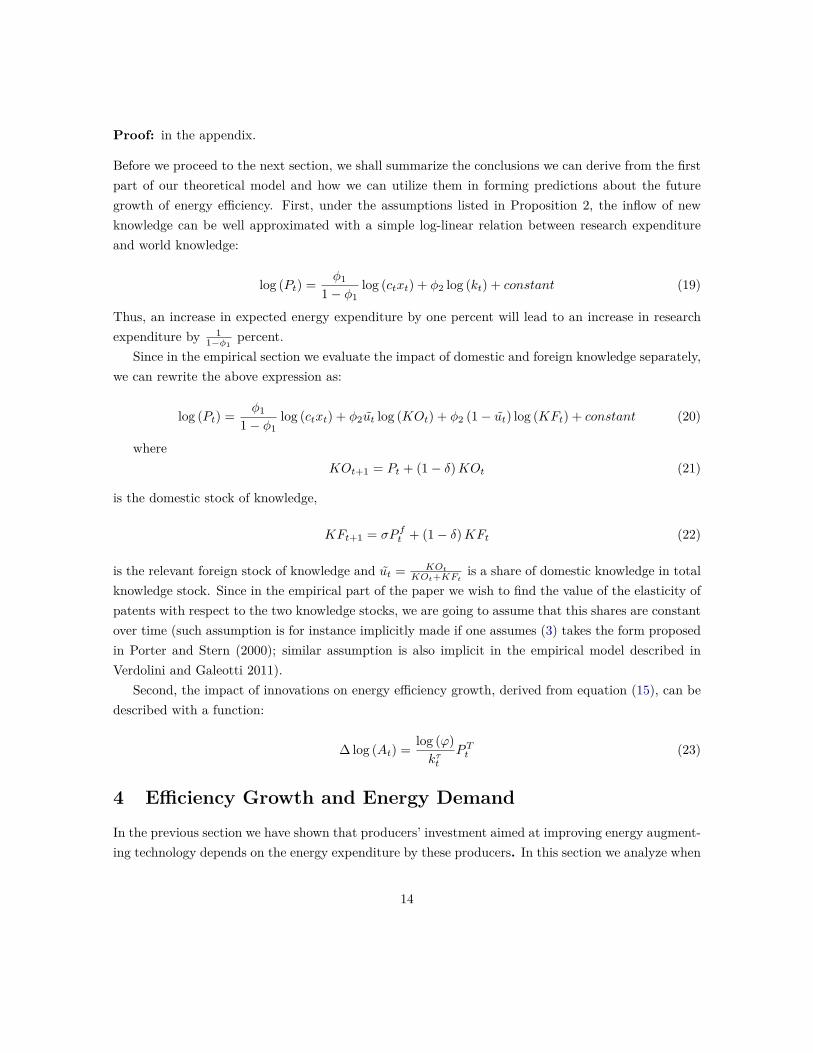
Before we proceed to the next section, we shall summarize the conclusions we can derive from the firstpart of our theoretical model and how we can utilize them in forming predictions about the futuregrowth of energy efficiency. First, under the assumptions listed in Proposition 2, the inflow of newknowledge can be well approximated with a simple log-linear relation between research expenditureand world knowledge:
log (Pt) = φ1
1− φ1log (ctxt) + φ2 log (kt) + constant (19)
Thus, an increase in expected energy expenditure by one percent will lead to an increase in researchexpenditure by 1
1−φ1percent.
Since in the empirical section we evaluate the impact of domestic and foreign knowledge separately,we can rewrite the above expression as:
log (Pt) = φ1
1− φ1log (ctxt) + φ2ut log (KOt) + φ2 (1− ut) log (KFt) + constant (20)
whereKOt+1 = Pt + (1− δ)KOt (21)
is the domestic stock of knowledge,
KFt+1 = σP ft + (1− δ)KFt (22)
is the relevant foreign stock of knowledge and ut = KOtKOt+KFt is a share of domestic knowledge in total
knowledge stock. Since in the empirical part of the paper we wish to find the value of the elasticity ofpatents with respect to the two knowledge stocks, we are going to assume that this shares are constantover time (such assumption is for instance implicitly made if one assumes (3) takes the form proposedin Porter and Stern (2000); similar assumption is also implicit in the empirical model described inVerdolini and Galeotti 2011).
Second, the impact of innovations on energy efficiency growth, derived from equation (15), can bedescribed with a function:
∆ log (At) = log (ϕ)kτt
PTt (23)
4 Efficiency Growth and Energy Demand
In the previous section we have shown that producers’ investment aimed at improving energy augment-ing technology depends on the energy expenditure by these producers. In this section we analyze when
14

improvement in energy augmenting technology can decrease the energy intensity of the economy andshift down the Marshallian demand for energy. In Section 3, we analyzed the possible functional formsdescribing the R&D process, however our conclusions did not rest on the choice of a specific form of theproduction function. Conversely, in this Section we need to specify the production function to carryout the modelling. Following other models on directed technological change (e.g. Andre and Smulders2014) we assume that output is produced using an energy intensive good x and non-energy-intensivegood, z, as follows:
y = (xρ + zρ)1ρ (24)
We assume that the non-energy-intensive good does not consume any energy. The energy intensivegood is produced using a continuum of intermediate goods:
x =
1ˆ
0
((Aixi)α z1−α
i
)σdi
1σ
The quality of the i’th intermediate is determined by the level of its technological advancement,Ai. Production of energy intensive intermediate good requires energy, xi , and the composite of otherinputs, zi. The producers of intermediates are monopolists. The assumption that energy intensivegood is produced with a continuum of intermediates supplied by monopolists is borrowed from theendogenous growth literature to ensure the existence of an equilibrium. The central role of thisassumption for the DTC models is discussed in Acemoglu (2007).
Monopolists can invest in improving the quality of a good. Their maximization problem can bestated as
maxpi,xi,Ri,
pi (Aixi)α z1−αi − cxi − wizi −Ri (25)
subject to
(Aixi)α z1−αi = p
σ1−σi´ 1
0 pσ
1−σj dj
p−1i (pex)
where pi is the quality adjusted price of intermediate i. As shown in the previous section, theoptimal R&D investment of monopolists i is going to be a log-linear function of energy expenditure :
logRi = k1 + 11− φ1
log (c′x′i)
If we assume that the initial level of technological advancement is the same for all energy intensiveintermediates, then they are exactly symmetric and they will all demand the same amount of energy(symmetry of sectors is a usual assumption in endogenous growth theory and DTC models - see e.g.
15

Dixit and Stiglitz (1977) and all subsequent models built on their framework, such as Romer (1987)and Acemoglu et al. (2012)):
xi = x
Since each monopolist faces the same energy expenditure, all monopolists have the same R&D spending,the same rate of technological advancement and the same level of A at any point in time.
Given that the elasticity of demand for intermediates with respect to quality-adjusted price isconstant each monopolist will charge the same mark-up over marginal costs. The quality adjustedprice of an intermediate is therefore
pi = µcαw1−α
Aα
where µ = 1σ
The producer of the energy intensive good, x, does not have a monopoly power and thus the priceit charges is equal to marginal cost, that is the quality-adjusted price of energy intensive intermediates:
px = pi = µcαw1−α
Aα
Finally, the optimization of the final good producer determines the demand for the energy intensivegood. Recalling that the price of final good is normalized to unity, the First Order Condition of thisproblem implies:
pxx = p−ρ
1−ρx y (26)
The Marshallian demand for energy in the economy can then be derived from the First OrderCondition to (25) with respect to energy:
x = αpxx
c= αc−1
(µcαw1−α
Aα
) −ρ1−ρ
y (27)
Simplifying and taking logs:
log (x) = log (y)−(
1 + αρ
1− ρ
)log (c)− (1− α) ρ
1− ρ log (w)
+ αρ
1− ρ log (A) + constant (28)
The increase in energy-augmenting technology will shift the Marshallian demand for energy downif the energy good is complementary to the non-energy good, that is, if ρ < 0.
We focus on the technological impacts on Marshallian demand because a similar function hasbeen used in the literature to forecast future energy demand (e.g. Webster, Paltsev and Reilly 2008,Schmalensee, Stoker and Judson 1998). Note that implicitly we also analyze the effect of A on the
16

energy intensity of the economy which could be easily derived from the Marshallian demand function:
log (x/y) = −(
1 + αρ
1− ρ
)log (c)− (1− α) ρ
1− ρ log (w) + ρ
1− ρ log (A) + 11− ρ log (µ)
The final step in solving the general equilibrium is to endogenize energy expenditure, which until nowhas been taken as exogenous. To do so, we could follow two strategies: we can merge our model withany large energy models, or, after making some additional assumption on the form of the productionfunction (24), solve the model analytically ourselves.
We prefer the former strategy. Hence, after estimating the model in the following section, in Section6 we merge it with an Integrated Assessment Model. However, for completeness, we also pursue thesecond strategy in the Appendix.
5 Empirical Analysis
5.1 Setup of the Empirical Model
In this Section, we empirically estimate the key parameters of the theoretical model set up above. Theempirical model, which will serve for calibration of the integrated assessment model, is derived directlyfrom the predictions of the theoretical model: the combination of equations (20), (23) and (28) can bepresented as a system of two equations (we restate them below for convenience):
log (Pt) = φ0 + φ1
1− φ1log (ct+1xt+1) + φ2u log (KOt) + φ2 (1− u) log (KFt) (29)
∆ log (x) = ∆ log (y)−(
1 + αρ
1− ρ
)∆ log (c)− (1− α) ρ
1− ρ ∆ log (w) + αρ
1− ρlog (ϕ)kτt−1
PTt (30)
We will first estimate the first equation and then use the fitted values to estimate the secondequation. This allows us to interpret the the coefficient in front of PT as the impact of inducedinnovations on energy demand.
To estimate the first equation we need to find the empirical proxies for the flow of new knowledge,P , the domestic knowledge stock, KO , the foreign knowledge stock, KF , and energy expenditurescx. Since in the model A stands for the productivity in production of energy intensive goods, P mustrefer to innovations that are relevant for energy intensive processes. Employment of the two stageestimator, described in more detail below, allows us to consider only a subset of relevant ideas. Thisis because any subset of ideas, if instrumented with energy expenditure, becomes representative of allthe ideas relevant for energy efficiency. Use of a subset rather than a total count of relevant ideas willtherefore not generate a measurement error bias. We use patent data as a proxy for the number ofideas that are novel in a country at time t. Specifically, we select patents classified in the following
17

IPC categories: Continuous Casting, Cement production, Combustion, Fuel cells, Heat exchange, Heatpumps, Injection, Metallurgical processes, Paper production, Stirling engines, Recovery of waste heat,Buildings and Lighting.
Turning to the other independent variables in the estimation of (29), the own knowledge stocksare built using patent data and the perpetual inventory method: KOt+1 = Pt + (1− δ)KOt andKFt+1 = σP f + (1− δ)KFt
Notice that this strongly resembles the specification in Peri (2005) and Verdolini and Galeotti (2011)although it has been derived from different micro-foundations. The foreign knowledge stock are alsobuilt following Verdolini and Galeotti (2011). For each country, the stock of available foreign knowledgeis defined as the sum of each foreign country’s knowledge weighted by the diffusion parameters whichare estimated in that study. We lag knowledge stocks by one years to control for the non-immediatediffusion of knowledge and to reflect the time lag between the year researchers work on innovation andthe year in which patent is applied for. The proxy for expenditures is constructed as the product oftotal energy supply and the ratio of energy price (Consumer Price Index for energy) to final good price(Consumer Price Index) and is lagged one year. We lag energy expenditure to take into account thatthe decision on R&D investment is based on past data.
To link the model to the empirical application we make two additional assumptions, in line withthe literature on patent data as proxy of innovative output. First, we assume that P is distributedPoisson with Poisson Arrival Rate λ = aRφ1kφ2Kφ3ε. Second, we assume that the Poisson ArrivalRate is itself a random variable. Its distribution is given by λ ∼ Gamma
(ϕ, aR
φ1kφ2
ϕ
)where ϕ is a
distribution parameter which can be estimated. These two assumptions imply that the distributionof patents is negative binomial. This is in line with previous literature, where the negative binomialdistribution is considered a good approximation of the patent count distribution observed in the data(Hausman, Hall and Griliches (1984)). The assumptions on the distribution of patents count enablesus to estimate equation (29) using Maximum Likelihood. In the baseline regression we have includeda vector of controls, x, which contain full set of country, time and patent category fixed effects. Theregression is therefore represented by the equation
Pist = exp [β0 + β1 log (cistxist) (31)
+β3 log (KOist) + β4 log (KFist) + x] ε+ η
where i indexes countries, s - patents categories and t - a year of patent application.Next, we turn to the empirical model which links number of patents and improvements in energy
efficiency, that is equation (30)As described in the theoretical section log (θ) could be interpreted as an innovative content of
patent. The content may depend on the number of innovations that has been produced in the field inthe past. ’Fishing out effect’ would predict a very large innovative content of each patent if the stock
18

of the previous patents is small; as the stock grows it is more and more difficult to produce a trulyinnovative patent. To examine this possibility we include the interaction term between the stock ofpatents and the number of new patents, i.e. we assume
log (ϕ)kτt−1
= δ1 + δ2TSit
where TS = KO +KF is the total stock of patents.Combining this result with equation 286:
∆ log (x) = ∆ log (y) + ρ
1− ργ2Pit + ρ
1− ργ3PitTSit
−(
1 + αρ
1− ρ
)∆ log (ct)−
(1− α) ρ1− ρ ∆ log (w)
We also assume that the price of other inputs, z, is equal to wages of labor and that it grows atthe same rate as the GDP. This is in line with the long-run dynamics of the balanced growth path,which we present in the Appendix. Based on this equation we propose an empirical model:
∆ log (x) = a1∆ log (y) + a2Pit + a3PitTSit + a4∆ log (ct) (32)
Therefore we examine the effect of energy saving patents on the energy consumption holding totalproduction and price of energy constant.
The alternative way of interpreting coefficient γ2 is an effect of energy saving patents on energyintensity:
∆ log(x
y
)= (a1 − 1) ∆ log (y) + a2Pit + a3PitTSit + a4∆ log (ct)
If the true production function has the CES form, γ1 = 1 and income has no effect on energyintensity. This result is a consequence of the homotheticity of the CES production function.
5.2 Data and Descriptive Statistics
The patent data used in the estimation of the first stage regression is taken from the PATSTATdatabase (EPO 2014). We select patent applications by inventor country and priority year, as cus-tomary in the literature, for technologies that reduce the demand for energy. These include Buildings,Cement combustion, Continuous casting, Fuel cells, Fuel injection, Heat exchange, Heat pump, Light-ing, Metallurgical processes, Paper production, Stirling engines and Waste heat recovery. The detailed
6Notice that pz is the price of inputs other than energy relative to the price of final good. Since price of energy isrelatively small component of the final good price, we approximate w = 1, thus log (w) = 0.
19

Variable Mean Std. Dev. Min MaxEnergy Consumption 126985 274550 2214 1581622Energy price index 81.68 14.13 37.91 137.36
Real GDP per capita 26620 10335 5051 80215Patents Count 112 255 0 1784Policy index 2.99 3.09 0 9
Table 1: Descriptive Statistics I: Mean, standard deviation and minimum and maximum values of thekey variables
list of IPC codes is presented in Appedix A.5. Patents are imperfect proxies of the output of innovativeactivity (Griliches 1990). The most relevant problem in our case is that patents greatly differ in theirquality (or inventive step), with the majority of patent having little value and a few having very highvalue. The skewed distribution of patent quality has been widely discussed in the literature. To ad-dress the concern that patent indicators in general may reflect innovation of low quality, in this paperwe select patent applications to the European Patent Office (EPO). Patent protection at the EPO isindicative that the patent applicant would like to exploit the innovation in more than one EPO memberstate, as application fees to the EPO are generally higher than those at national offices, but lower thanfiling in multiple countries. Considering EPO applications should hence provide a quality thresholdto proxy for innovation. In any case, we provide robustness checks by considering applications to theUSPTO and through the Patent Cooperation Treaty. .
Energy price indexes for household and industry are taken from the IEA Energy Prices and TaxesDatabase (IEA 2013a), while data on Total Final Energy Consumption in ktoe is taken from theIEA World Energy Balances Database (IEA 2013b). In addition, the second stage regression usesinformation on GDP per capita in PPP taken from the Penn World Tables version 7.1 and convertedin constant prices. In the first stage regression we also include a variable proxying for the stringencyof policies supporting increases in the efficiency of energy use in a given country in a given year. Thisis build using data from the WEO Energy Efficiency Policy Database (IEA 2014). Specifically, wecollect information on what type of policy instrument is used to target energy efficiency in any givencountry at a give time. The type of instruments considered are: Investments, Feed-in-Tariffs, Taxes,Certificates, Educational programs, General policies, Obbligations, R&D investments and Voluntarymeasures. We assign a value of 1 to each indicator once it is implemented. We then sum the indicatorsfor each country and each year. We resort to such indicator due to the difficulty of building morecomplex numerical measures of environmental policy stringency which cover a wide range of differentpolicy instrument. While very crude, similar proxies have been used in the literature (see for instanceNesta et al. 2014) and arguably capture a signal given to investors that governments are committingto tackling energy efficiency by increasing the complexity of the policy portfolio.
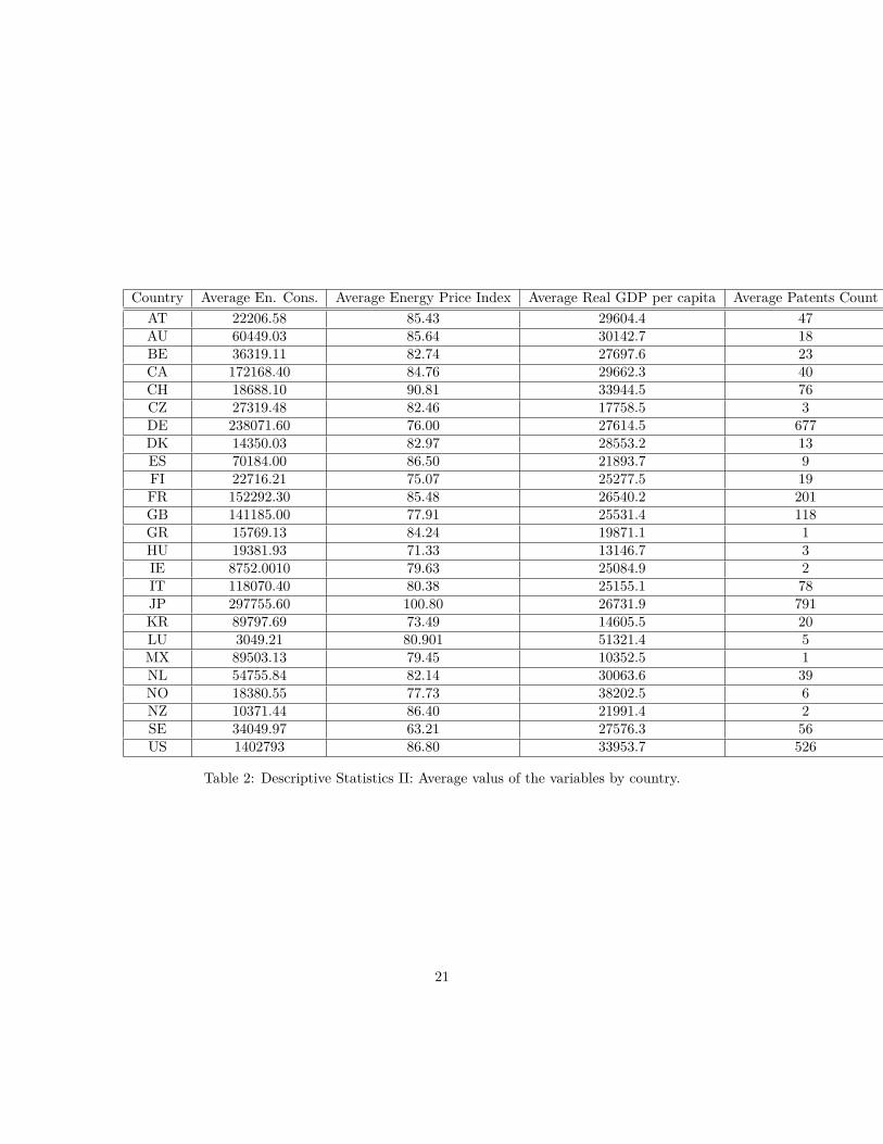
Tables 1 and 2 provide descriptive statistics of the main variables for each country in our sample.
20
Country Average En. Cons. Average Energy Price Index Average Real GDP per capita Average Patents CountAT 22206.58 85.43 29604.4 47AU 60449.03 85.64 30142.7 18BE 36319.11 82.74 27697.6 23CA 172168.40 84.76 29662.3 40CH 18688.10 90.81 33944.5 76CZ 27319.48 82.46 17758.5 3DE 238071.60 76.00 27614.5 677DK 14350.03 82.97 28553.2 13ES 70184.00 86.50 21893.7 9FI 22716.21 75.07 25277.5 19FR 152292.30 85.48 26540.2 201GB 141185.00 77.91 25531.4 118GR 15769.13 84.24 19871.1 1HU 19381.93 71.33 13146.7 3IE 8752.0010 79.63 25084.9 2IT 118070.40 80.38 25155.1 78JP 297755.60 100.80 26731.9 791KR 89797.69 73.49 14605.5 20LU 3049.21 80.901 51321.4 5MX 89503.13 79.45 10352.5 1NL 54755.84 82.14 30063.6 39NO 18380.55 77.73 38202.5 6NZ 10371.44 86.40 21991.4 2SE 34049.97 63.21 27576.3 56US 1402793 86.80 33953.7 526
Table 2: Descriptive Statistics II: Average valus of the variables by country.
21

For our empirical estimation we compute energy expenditures using information on energy priceindexes and energy consumption. We also create variables to proxy for the own and foreign knowledgestocks. Own and foreign knowledge stocks are created using the perpetual inventory method as in Peri(2005) and in accordance with equations (21) and (22) with a discount rate of 0.15. To build foreignknowledge stock we weight the stock of other countries using the international knowledge spilloversparameters estimated in Verdolini and Galeotti (2011)7. Finally, in the second stage regressions GDPper capita and second stage energy price and consumption are smoothed using HP filter to removeshort term variation.
Estimating equation (31) with knowlege stock variables in logs means that if the stocks are zero,the log is not defined. To address this, in we introduce two dummy variables which takes the value 1if the respective stock of knowledge is zero.
5.3 Results
The results emerging from the estimations of (31) are summarized in Table 3. All models includetechnology, country and time fixed effects. k. Column 1 shows the results of a reduced model wherepatent counts is regressed on expenditure. The coefficient on energy expenditure is close to unity andhighly statistically significant. Inclusion of GDP per capita as a control variable (column 2) does notalter this results significantly.
Column 3 shows the results of the model including all determinants of innovation as emergingfrom our theoretical model: energy expenditure, own knowledge stock and foreign knowledge stock.The coefficient on energy expenditure falls to 0.53, that is an increase in energy expenditure by 10%leads to 5.3% increase in number of patents. The coefficient remains significant at 1% significancelevel. Significant coefficient on own knowledge are in line with the findings of Verdolini and Galeotti(2011), Popp (2002) and Porter and Stern (2005). Increase in own knowledge stock by 10% increasesgeneration of patented ideas by 6.3%, which is very close to the results obtained by Popp (2002). Theresults confirm also the role of foreign knowledge spillovers for the domestic innovation process. A 10percent increase in foreign knowledge increases innovation by roughly 1.8 percent. To reduce the riskof bias due to omitted variable, in columns 4 and 5 we include GDP per capita and a policy index thatcounts major environmental policies present in a country at given point in time. The inclusion of thesetwo regressors neither changes the signs nor the significance level of the coefficients. However, thecoefficient on energy expenditure is smaller. As expected, both GDP and policy index has a positiveand significant effect on energy saving patents.
To get a flavor of the economic implications of this result, we may combine them with the predictionsof the U.S. Energy Information Administration (EIA 2014). The EIA predicts that the real energy
7applying weights to patents from different countries is effectively accounting for the presence of parameter σ inequation (22)
22

expenditure will increase by 21% between 2005 and 2040. According to our estimates, this wouldinduce the total annual flow of patents available for US economy by 7%: from 1298 to 1393. However,this calculations ignore the effects of spillovers, which might have an additional positive effect ongeneration of patents.
We provide some robustness checks by running similar regression with different patent counts(see Table 6 in the Appendix). Specifically, we use the count of PCT applications and the countof patents granted by the USPTO. - Results are similar to those presented in table 3 except in theUSPTO specification, where the coefficient on energy expenditures is still positive but does not reachan acceptable level of significance.
.The models presented so far use dynamics in aggregate expenditures as a proxy for the dynamics
in energy expenditures of energy intensive sectors. The assumption behind such an empirical choice isthat energy consumed in energy intensive processes is proportional to total energy consumption in theeconomy, hence using the second can inform on the effect of the first on innovation. This assumption ismore likely to hold at more disaggregated level, i.e. if for the industrial patents we will use industrialenergy use, while for the household related patents (such as lighting) we use household energy use..Therefore, we regress patents related to energy intensive processes in industrial production8 on energyexpenditure in industry and patents related to household energy intensive processes 9 on residentialenergy expenditure. The results are reported in Table 4. The signs of all coefficients are in linewith the theoretical predictions. A ten percent increase in industrial energy expenditure correspondsto an increase in the patents count by 2.2%. The effect is lower then predicted in the regressionwith aggregated expenditure, but its economic significance remains substantial. We also find thatresidential energy expenditure is positively correlated with household related energy patents. However,the coefficient is not statistically significant.
Next we examine the effect of induced innovation on actual energy savings. In this second stageregression, we use the predicted innovation levels fitted using the model specified in column 4 in table3. The estimates, reported in Table 5, implies that a thousand additional “induced” patents, whichis approximately the total annual flow of new patents available for US economy in 2010, lead to a0.52% decline in energy intensity. Note that the average annual decline of US energy intensity in years2009-2011 was 1.87%. This implies that induced directed technological change can explain around onethird of the total decline in US energy intensity. The effect is statistically significant at the 10% level(if standard errors are computed by clustering at country level). Using PCT applications, the resultis of similar magnitude but more precisely estimated (Table 8 in the Appendix, columns (1) and (2)):.a thousand induced patents lead to a 0.60 percent decline in energy intensity. The estimated effect in
8The patent’s categories included in this group are Continues Casting, Cement production, Combustion, Fuel Cell,Heat Exchange, HeatPump, Injection, Metallurgical processes, Paper production, Stirling engines, recovery of wasteheat.
9The patent’s categories included in this group are buildings and lighting.
23

the USPTO specification is 0.18%. (Table 8 in the Appendix, columns (3) and (4)).Putting this in perspective using the EIA predictions we find that additional 95 patents per year
induced by increased energy expenditure by 2040 (which we calculated from the first stage regression)would translate into an increase in the annual energy efficiency growth rate by 0.05 percentage point.This implies that, if growth of GDP and growth of energy price in 2040 is the same as in 2011, theenergy intensity decline would increase from 1.87% to 1.92% per annum. Again, this simple calculationsignore the effect of spillovers. They also do not take into account that energy efficiency growth wouldreduce the consumption of energy and energy expenditure. Accounting for these effects is not easythrough a simple calculation. Hence, we accounted for this effects in the counter-factual exercisepresented in Section 6.
In Table 5, column (2) we test whether the data shows evidence for the “fishing out effect” inenergy saving R&D, i.e. whether the effect of patents decline with the accumulation of world knowledgestock. Since the coefficient on the interaction term between the stock and patents has a negative signwe conclude that there is no evidence for the fishing out effect. This means that the effect of a patenton a growth of energy efficiency does not depend on how many patents have been invented in past. Inother words patent in 2005 has the same effect of energy efficiency growth rate as the patent inventedin 80s. Note that our result is restricted to the patents in energy intensive sectors and may not holdin the entire economy.
Finally, as for the first stage regression, we present the results of the disaggregated analysis forindustry and household samples. For industry , the estimates implies that one thousand additionalpatents arising due to energy expenditure growth lead to a 0.535% decline in energy consumption.The effect is statistically significant at 10% significance level. For the household data, the effect ismuch more substantial: a hundred patents “induced” patents decrease the energy demand by 16.2%,although it is not statistically significant. One potential explanation for this pattern is that the effectin industry is limited by the effect of patents on international competitiveness: an increase in efficiencyin energy intensive sectors in one country implies that these sectors become more competitive relativeto similar sectors in other countries. This leads to an increase in global market share of the moreefficient firms, in the production and hence in the demand for energy. As a result initial energy savingsmay be partly offset and the total effect is weak.
6 Merging with Integrated Assessment Model
The final section of this paper has two objectives. First, it illustrates the quantitative impact ofDirected Technological Change on future energy efficiency growth. Second, it allows us to close thetheoretical model by endogenizing energy expenditure, which has been assumed exogenous in sections3 and 4.
To do so we merge our model with the WITCH Integrated Assessment Model (Bosetti et al. (2009)).
24

Granted EPO(1) (2) (3) (4) (5)
energy expenditure 1.523*** 1.113*** 0.532*** 0.363*** 0.378***[0.111] [0.131] [0.0903] [0.102] [0.102]
own knowledge 0.655*** 0.656*** 0.656***[0.0135] [0.0136] [0.0136]
foreign knowledge 0.182*** 0.180*** 0.179***[0.0314] [0.0314] [0.0313]
GDP per capita 1.549*** 0.787*** 0.786***[0.225] [0.171] [0.171]
policy index 0.0192**[0.00898]
Table 3: The dependent variable is the count of patents in energy intensive technologies. ***, **, * indicate significanceof the coefficients at the 1%, 5% and 10% level, respectively. All regressions contain full set of country, time and patentscategory dummy variables. All variables are transformed with a log function. The estimations are obtained using aMaximum Likelihood estimator. The probability distribution assumed is the negative binomial. Standard errors arereported in parenthesis.
Granted EPOaggregate industry household
(1) (2) (3)energy expenditure 0.363*** 0.222*** 0.156
[0.102] [0.0604] [0.442]own knowledge 0.656*** 0.666*** 0.442***
[0.0136] [0.0143] [0.0584]foreign knowledge 0.180*** 0.207*** 0.385***
[0.0314] [0.0326] [0.141]GDP per capita 0.787*** 0.874*** 1.996***
[0.171] [0.158] [0.704]
Table 4: The dependent variable is the count of patents in energy intensive technologies . ***, **, * indicate significanceof the coefficients at the 1%, 5% and 10% level, respectively. All regressions contain full set of country, time and patentscategory dummy variables. All variables are transformed with a log function . The estimations are obtained using aMaximum Likelihood estimator. The probability distribution assumed is the negative binomial. Standard errors arereported in parenthesis.
25
Granted EPOtotal industry household
(1) (2) (3) (4) (5) (6)GDP growth 0.499*** 0.494*** 0.499*** 0.494*** 0.503*** 0.505***
[0.0793] [0.0804] [0.0793] [0.0804] [0.0791] [0.0791]Price growth -0.0953** -0.102*** -0.0949** -0.102*** -0.104*** -0.103***
[0.0350] [0.0357] [0.0352] [0.0360] [0.0336] [0.0333]total patents count -0.00518* -0.000107 -0.00535* 1.35e-05 -0.162 -0.206*
[0.00274] [0.00353] [0.00279] [0.00363] [0.121] [0.119]patents X Stock -0.00322 -0.00338 0.515
[0.00220] [0.00215] [1.113]constant 0.00523** 0.00350 0.00525** 0.00345 0.00457** 0.00493**
[0.00207] [0.00213] [0.00207] [0.00213] [0.00206] [0.00200]
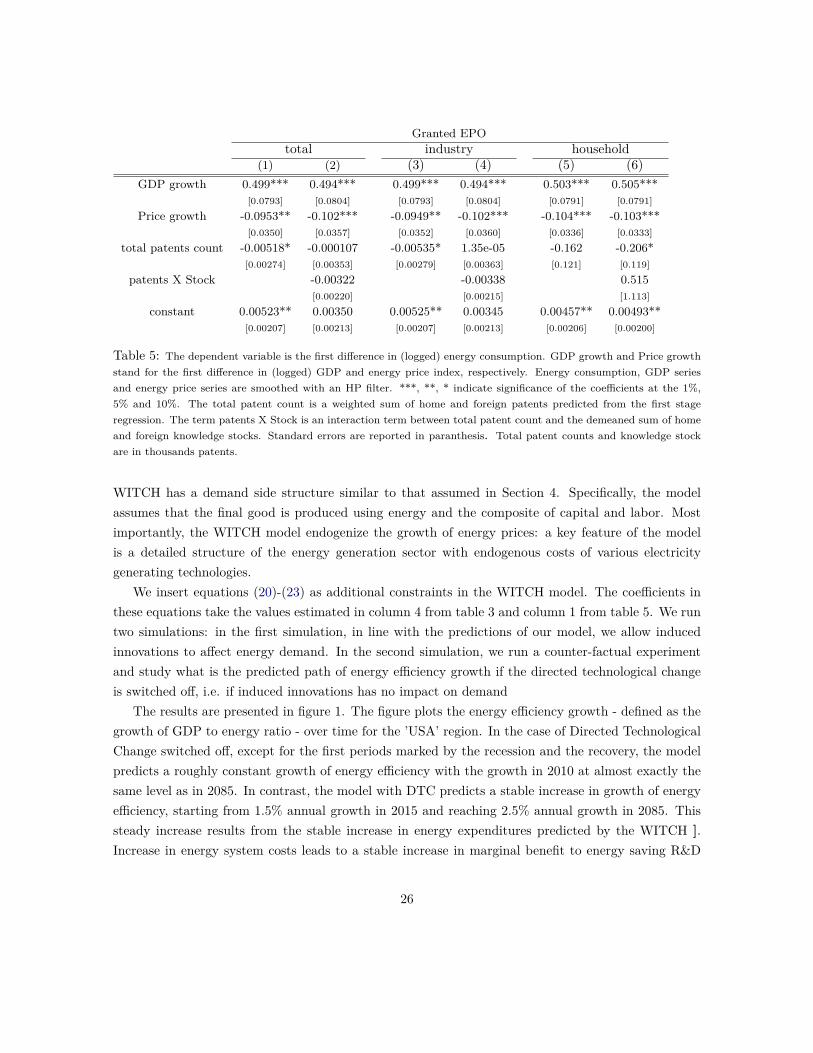
Table 5: The dependent variable is the first difference in (logged) energy consumption. GDP growth and Price growthstand for the first difference in (logged) GDP and energy price index, respectively. Energy consumption, GDP seriesand energy price series are smoothed with an HP filter. ***, **, * indicate significance of the coefficients at the 1%,5% and 10%. The total patent count is a weighted sum of home and foreign patents predicted from the first stageregression. The term patents X Stock is an interaction term between total patent count and the demeaned sum of homeand foreign knowledge stocks. Standard errors are reported in paranthesis. Total patent counts and knowledge stockare in thousands patents.
WITCH has a demand side structure similar to that assumed in Section 4. Specifically, the modelassumes that the final good is produced using energy and the composite of capital and labor. Mostimportantly, the WITCH model endogenize the growth of energy prices: a key feature of the modelis a detailed structure of the energy generation sector with endogenous costs of various electricitygenerating technologies.
We insert equations (20)-(23) as additional constraints in the WITCH model. The coefficients inthese equations take the values estimated in column 4 from table 3 and column 1 from table 5. We runtwo simulations: in the first simulation, in line with the predictions of our model, we allow inducedinnovations to affect energy demand. In the second simulation, we run a counter-factual experimentand study what is the predicted path of energy efficiency growth if the directed technological changeis switched off, i.e. if induced innovations has no impact on demand
The results are presented in figure 1. The figure plots the energy efficiency growth - defined as thegrowth of GDP to energy ratio - over time for the ’USA’ region. In the case of Directed TechnologicalChange switched off, except for the first periods marked by the recession and the recovery, the modelpredicts a roughly constant growth of energy efficiency with the growth in 2010 at almost exactly thesame level as in 2085. In contrast, the model with DTC predicts a stable increase in growth of energyefficiency, starting from 1.5% annual growth in 2015 and reaching 2.5% annual growth in 2085. Thissteady increase results from the stable increase in energy expenditures predicted by the WITCH ].Increase in energy system costs leads to a stable increase in marginal benefit to energy saving R&D
26

0.00%
0.50%
1.00%
1.50%
2.00%
2.50%
3.00%
3.50%
2010 2015 2020 2025 2030 2035 2040 2045 2050 2055 2060 2065 2070 2075 2080 2085 2090
no DTC
DTC
Figure 1: Effect of induced innovations on energy efficiency
investment and increase in the flow of energy saving patents. Greater innovativeness translates intohigher energy efficiency growth.
The prediction of stable increase in growth rate may resemble the scale effect which has beennoted and criticized by Jones (1995) in the context of TFP growth. Jones argued that while the firstgeneration of endogenous growth models predicted an increase in the TFP growth rate after increase inthe size of population, no such effect was observed in data. Jones then suggested that the mispredictionof endogenous growth models originates from ignoring the fishing-out effect, i.e. fall in the quality ofinnovations over time. Note however, that we did allow for fishing out effects in our regressions andwe did not find any evidence for the decrease in value of innovations despite the fact that number ofpatents in our sample was growing over time . This may suggest that energy efficiency growth, incontrast to the TFP growth, is robust to Jones criticism and may feature scale effect.
7 Conclusions
The aim of this paper was to study the drivers and consequences of price-induced technological changein the efficiency of energy use. First, we derived a theoretical model describing how innovation maybe induced by changes in energy expenditure and how the flow of new ideas may turn into energyefficiency gains. We then quantified the links between energy expenditure and innovations and between
27

innovations and energy efficiency using an empirical model. In the last step, we used the empiricalresults to forecast future energy efficiency growth.
In the theoretical model we show that under very general assumptions information about energyexpenditures, knowledge spillovers and the parameters governing the R&D process are sufficient topredict the R&D effort in efficiency-improving technologies. Then we pinned down the conditionsfor a log-linear relation between energy expenditure and the R&D effort. As long as the decisionmaker in the model assumes constant growth of energy expenditures in future periods and if log-linearrelation between energy efficiency gain and R&D investment is assumed, the equilibrium choice of R&Dinvestment is proportional to energy expenditure. If, instead, we assume that growth of efficiency isproportional to the number of inventions and production of inventions is a Cobb-Douglas function ofR&D investment 10, then the equilibrium choice of R&D investment becomes a log-linear function ofenergy expenditure.
In section 4 we find that the productivity improvements in energy intensive sectors shifts theMarshallian demand for energy downward. Since efficiency growth can be derived as a linear functionof the flow of innovations, we arrive to the simple relation between change in demand for energy andpatent counts.
To estimate the model we follow a two-stage estimation procedure. The first stage examinesthe effect of energy expenditures and spillovers on energy saving patents; the second stage uses thepredicted innovation values from the first stage to study the impact of induced innovation on the energydemand. The result for the first stage predicts that a 10% increase in energy expenditure leads to a3.6% increase patents. The result is robust to inclusion of country, time and technology specific fixedeffects, controls for income and policy. The model predicts a statistically significant relation betweenproduction of patents and accumulation of past knowledge , both within the country and abroad. 10%increase in the stock of past patents increases the probability of patenting by 6.5%. Regarding thesecond stage, the flow of patents is negatively correlated with the growth of energy demand. The pointestimates suggest that an increase in number of patents by a thousand leads to a 0.52% reduction inenergy use. We do not find any evidence for the fishing-out effect: increase in the stock of past patentsdoes not have any negative effect on the energy-saving impact of new patents.
Acknowledgements
The research leading to these results has received funding from the European Union Seventh FrameworkProgramme (FP7/2007-2013) under grant agreements n° 308481 (ENTRACTE) and and n° 308329
(ADVANCE)
10This is a specification analogous to Caballero and Jaffe (1993).
28

We are grateful to participants of conferences and workshops in Vienna, Milan, Venice, Paris and Utrecht andtwo anonymous referees for their constructive comments and valuable suggestions.
References
• Acemoglu, D. (1998). "Why Do Technologies Complement Skills? Direct Technical Change andWage Inequality", Quarterly Journal of Economics, 113, 1055-1090.
• Acemoglu, D. (2000). "Technical Change, Inequality, and the Labor Market," NBER WorkingPapers 7800, National Bureau of Economic Research, Inc.
• Acemoglu, D. (2007). "Equilibrium Bias of Technology," Econometrica, Econometric Society, vol.75(5), pages 1371-1409, 09.
• Acemoglu, D. (2014). "Localized and Biased Technologies: Atkinson and Stiglitz’s New View, In-duced Innovations, and Directed Technological Change," NBER Working Papers 20060, NationalBureau of Economic Research, Inc.
• Acemoglu, Daron, Ufuk Akcigit, Douglas Hanley and William Kerr, 2014. "Transition to CleanTechnology," NBER Working Papers 20743, National Bureau of Economic Research, Inc.
• Acemoglu, Daron, Philippe Aghion, Leonardo Bursztyn and David Hemous, 2012. "The En-vironment and Directed Technical Change," American Economic Review, American EconomicAssociation, vol. 102(1), pages 131-66, February.
• Aghion, Philippe and Peter Howitt, 1992. "A Model of Growth through Creative Destruction,"Econometrica, Econometric Society, vol. 60(2), pages 323-51, March.
• Anderson, S. T., R. Kellogg, J. M. Sallee and R. T. Curtin, 2011. “Forecasting Gasoline PricesUsing Consumer Surveys”. American Economic Review, 101(3):110–14.
• André, F.J. and S. Smulders (2014)."Fueling growth when oil peaks: Directed technologicalchange and the limits to efficiency," European Economic Review, Elsevier, vol. 69(C), pages18-39.
• Bosetti, Valentina, Carlo Carraro, Romain Duval, Alessandra Sgobbi and Massimo Tavoni, 2009."The Role of R&D and Technology Diffusion in Climate Change Mitigation: New PerspectivesUsing the WITCH Model," OECD Economics Department Working Papers 664, OECD Publish-ing.
• Bosetti, Valentina, Emanuele Masseti and Massimo Tavoni (2007). "The WITCH Model: Struc-ture, Baseline, Solutions". FEEM Working Paper Series No. 10-2007.
29

• Bosetti, Valentina and Elena Verdolini, 2013. "Clean and Dirty International Technology Diffu-sion," Working Papers 2013.43, Fondazione Eni Enrico Mattei.
• Caballero, Ricardo J and Adam B. Jaffe, 1993. "How High are the Giants’ Shoulders: AnEmpirical Assessment of Knowledge Spillovers and Creative Destruction in a Model of EconomicGrowth," NBER Chapters, in: NBER Macroeconomics Annual 1993, Volume 8, pages 15-86National Bureau of Economic Research, Inc.
• Goulder, L.H., Schneider, S. (1999). “Induced technological change and the attractiveness ofCO2 abatement policies.” Resource and Energy Economics 21, 211-253.
• Dixit, Avinash K and Joseph E. Stiglitz, 1977. "Monopolistic Competition and Optimum ProductDiversity," American Economic Review, American Economic Association, vol. 67(3), pages 297-308, June.
• U.S. Energy Information Administration (2014), ”Annual Energy Outlook 2014”,
• EPO, 2014. EPO Worldwide Patent Statistical Database (PATSTAT), April 2014 release
• Griliches, Zvi, 1990. "Patent Statistics as Economic Indicators: A Survey," Journal of EconomicLiterature, American Economic Association, vol. 28(4), pages 1661-1707, December.
• Grossman, Gene M and Elhanan Helpman, 1991. "Quality Ladders in the Theory of Growth,"Review of Economic Studies, Wiley Blackwell, vol. 58(1), pages 43-61, January.
• Hassler, John, Per Krusell and Conny Olovsson, 2012. "Energy-Saving Technical Change," NBERWorking Papers 18456, National Bureau of Economic Research, Inc.
• Hausman, Jerry A., Bronwyn H. Hall and Zvi Griliches, 1984. "Econometric Models for CountData with an Application to the Patents-R&D Relationship," NBER Technical Working Papers0017, National Bureau of Economic Research, Inc.
• EIA U.S. Energy Information Agency, 2011. “Annual Energy Review 2011”
• IEA, 2013a. IEA Energy Prices and Taxes Database
• IEA, 2013b. World Energy Balances Database
• IEA, 2014. World Energy Outlook Policy Databases
• IEA, 2015. Energy Technology Perspective, Paris
• Jones, Charles I, 1995. "R&D-Based Models of Economic Growth," Journal of Political Economy,University of Chicago Press, vol. 103(4), pages 759-84, August.
30
• Joutz, Frederick L. and Yasser Abdih, 2005. "Relating the Knowledge Production Functionto Total Factor productivity: An Endogenous Growth Puzzle," IMF Working Papers 05/74,International Monetary Fund.
• Nesta, L., Vona, F., Nicolli, F., 2014. Environmental Policies, Competition and Innovation inRenewable Energy, Journal of Environmental Economic and Management vol. 67(3), pp. 396-411.
• Noailly, J. and R. Smeets, 2013. "Directing Technical Change from Fossil-Fuel to RenewableEnergy Innovation: An Empirical Application Using Firm-Level Patent Data," Working Papers2013.34, Fondazione Eni Enrico Mattei.
• Peri, Giovanni, 2005. "Determinants of Knowledge Flows and Their Effect on Innovation," TheReview of Economics and Statistics, MIT Press, vol. 87(2), pages 308-322, May.
• Popp, David, 2001. "The effect of new technology on energy consumption”. Resource and EnergyEconomics 23(3), pages 215-239.
• Popp, David, 2002. "Induced Innovation and Energy Prices," American Economic Review, Amer-ican Economic Association, vol. 92(1), pages 160-180, March.
• Porter, Michael E. and Scott Stern, 2000."Measuring the ’Ideas’ Production Function: Evidencefrom Internationa Patent Output", NBER working paper 7891, National Bureau of EconomicResearch, Inc.
• Rivera-Batiz, Luis A. and Paul M. Romer, 1991. "Economic Integration and Endogenous Growth,"The Quarterly Journal of Economics, MIT Press, vol. 106(2), pages 531-55, May.
• Romer, Paul M, 1986. "Increasing Returns and Long-run Growth," Journal of Political Economy,University of Chicago Press, vol. 94(5), pages 1002-37, October.
• Romer, Paul M, 1987. "Growth Based on Increasing Returns Due to Specialization," AmericanEconomic Review, American Economic Association, vol. 77(2), pages 56-62, May.
• Romer, Paul M, 1990. "Endogenous Technological Change," Journal of Political Economy, vol.98(5), pages S71-102, October.
• Sorrell, Steve. (2009). "Jevons’ Paradox revisited: The evidence for backfire from improvedenergy efficiency," Energy Policy, Elsevier, vol. 37(4), pages 1456-1469, April.
• Sue Wing, I. (2008). “Explaining the declining energy intensity of the U.S. economy”. Resourceand Energy Economics 30(1), 21–49.
31

• Stiglitz, Joseph and Linda J. Bilmes, 2015. “The Book of Jobs”. http://www.vanityfair.com/news/2012/01/stiglitz-depression-201201 (accessed on 31st March 2015)
• Verdolini, Elena and Marzio Galeotti, 2011. "At home and abroad: An empirical analysis ofinnovation and diffusion in energy technologies," Journal of Environmental Economics and Man-agement, Elsevier, vol. 61(2), pages 119-134, March.
• Young, Alwyn, 1998. "Growth without Scale Effects", Journal of Political Economy, Vol. 106,No. 1 (February 1998), pages 41-63
• Richard Schmalensee, Thomas M. Stoker and Ruth A. Judson, 1998. "World Carbon DioxideEmissions: 1950-2050," The Review of Economics and Statistics, MIT Press, vol. 80(1), pages15-27, February.
Appendix
A1. Endogenous Wages.
Let
P = a(bφ1 (L∗R)αφ1
(LER)(1−α)φ1
)kφ2
where L∗R denotes unspecialized labour which can be hired at fixed wage from the labour market.We assume that the energy market is too small to affect the wages of the unspecialized labour. LERdenotes labour specialized in the energy saving research, which is supplied inelastically. In this casethe firm, in addition to choosing its total expenditure needs to choose also the share of expendituredevoted for the external scientists and the internal scientists. This problem can be written as:
min {w∗RL∗R + w∗EL∗E}
subject to b (L∗R)α(LER)1−α = R, where R is determined in equation 12. The first order conditions
implythen
w∗RL∗R = αR
wERLER = (1− α)R
32

and
P = a
(R
(w∗R)α(wER)1−α
)φ1
kφ2
If LER and w∗R are fixed, then
P = a
((R
w∗R
)α(LER
1− α
)(1−α))φ1
kφ2
if wages are proportional to GDP, then equation 19 can be written as
log (Pt) = αφ1
1− φ1log (ctxt) + φ2 log (kt)− φ1α log (y) + constant
A1. Radical Innovations
It is also possible to interpret the function (15) as a sequence of radical innovations, where the sizeof innovations in each year is random. To see this, notice that the equation above can be reexpresedwith11
At =(
1 + log (θ)(PTt)ν)
At−1 (33)
As described in the technical appendix ’Radical Innovations’, the rationale behind such specificationis as follows: Suppose that each year brings Pt potential innovation. Each innovation may improveefficiency by factor µ, with µ being a random variable distributed with Frechet distribution with thescale parameter ϕ, shape parameter v and location parameter m = 1. Suppose that each year onlythe best innovation is chosen and implemented. In this case the efficiency next period is going to takethe form:
At =(
1 + log (θ)(PTt)ν)
At−1 (34)
which correspends to the expression (33).
A2. Reduced form of the Efficiency Gain Functional Form
We first show that assuming the functional form (15) does not change the first order condition statedin equation (9). We restate equation (15) below for convinience:
At =(ˆ Nt
−∞(xt (q) θq)α dq
) 1α
Multiplying it by the total amount of energy:11using the approximation ∆ log (At) = ∆At
At−1
33

Ax =(ˆ Nt
−∞(x (q) θq)α dq
) 1α
FOCs to energy in different processes:
∂y (Ax, z)∂Ax
(ˆ Nt
−∞(x (q) θq)α dq
) 1α−1
x (q)α−1 (θq)α = px
This could be also expressed as:
∂y (Ax, z)∂Ax
(ˆ Nt
−∞(x (q) θq)α dq
) 1α−1
(x (q))α−1 (θq)α = px (35)
∂y (Ax, z)∂Ax
(ˆ Nt
−∞(x (q) θq)α dq
) 1α−1
(x (q) θq)α = pxx (q)
Multiplying both sides by x (q) and integrating over q’s
ˆ Nt
∞
∂y (Ax, z)∂Ax
(ˆ Nt
−∞(x (q) θq)α dq
) 1α−1
(x (q) θq)α dq =ˆ Nt
∞pxx (q) dq
∂y (Ax, z)∂Ax
(ˆ Nt
−∞(x (q) θq)α dq
) 1α−1 ˆ Nt
∞(x (q) θq)α dq = px
ˆ Nt
∞x (q) dq
∂y (Ax, z)∂Ax
(Aα)1α−1
Aα = px
∂y (Ax, z)∂Ax
x = pxx
A
which is the same as the original FOC with respect to energy at the beginning of the theory section.Regarding individual x (q)’s, using (35):
∂y (Ax, z)∂Ax
(ˆ Nt
−∞(x (q) θq)α dq
) 1α−1
(x (q))α−1 (θq)α = px
34

which can be reduced to
pxA
(Aα)1α−1 (x (q))α−1 (θq)α = px
Rearranging: (θq
A
) α1−α
= x (q)
and comparing to the frontier innovation:
x (q)x (N) = θ−
α1−α (N−q)
Applying this to the definition of A in (15)
At =(ˆ Nt
−∞(x (q) θq)α dq
) 1α
At =(ˆ Nt
−∞
((θq
A
) α1−α
θq
)αdq
) 1α
Rearranging terms:
A1
1−αt =
(ˆ Nt
−∞
(e
log(θ)1−α αq
)dq
) 1α
The integration results in
A1
1−αt =
[(e log(θ)1−α αq
log(θ)1−α α
)]Nt−∞
1α
A1
1−αt =
(e
log(θ)1−α αNt
log(θ)1−α α
) 1α
Rearraning this gives:
35
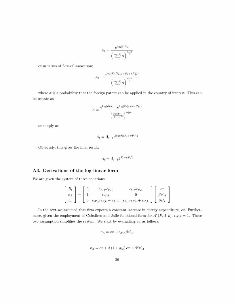
At = elog(θ)Nt(log(θ)1−α α
) 1−αα
or in terms of flow of innovation:
At = elog(θ)(Nt−1+Pt+σPft)(log(θ)1−α α
) 1−αα
where σ is a probability that the foreign patent can be applied in the country of interest. This canbe restate as
A = elog(θ)Nt−1elog(θ)(Pt+σPft)(log(θ)1−α α
) 1−αα
or simply as
At = At−1elog(θ)(Pt+σPft)
Obviously, this gives the final result:
At = At−1θPt+σPft
A3. Derivations of the log linear form
We are given the system of three equations: Rt
vA
vk
=
0 εA′P εPR εk′P εPR
1 εA′A 00 εA′,P εP,k + εA′,k εk′,P εP,k + εk′,k
cx
βv′A
βv′k
In the text we assumed that firm expects a constant increase in energy expenditure, cx. Further-
more, given the employment of Caballero and Jaffe functional form for A′ (P,A, k), εA′A = 1. Thesetwo assumption simplifies the system. We start by evaluating vA as follows:
vA = cx+ εA′Aβv′A
vA = cx+ β (1 + gcx) cx+ β2v′A
36

vA = cx
1− β (1 + gcx)
Note this is finite if the energy expenditure growth is not too fast. Note also that v′A = (1 + gcx) vA.Next, we turn to vk
vk = (εA′,P εP,k + εA′,k)βv′A + (εk′,P εP,k + εk′,k)βv′k
Using the assumed functional forms and resulting elasticities:
vk = (gAφ2 − τgA)βv′A +((
1− 1− δ1 + gk
)uφ2 + 1− δ
1 + gk
)βv′k
vk = gA (φ2 − τ) (1 + gcx)βvA +(uφ2 + (1− uφ2) 1− δ
1 + gk
)βv′k
Now, note that in the long run the economy approaches its balanced growth path characterizedby gk = gP (where tilda denotes the long run growth rate). thus unless the economy at time t is atthe point that is very distant from that balanced growth path, in period t+ 2 gk′ ≈ gk. On this path1+ gk = 1+ gP = 1
1−φ11
1−φ2ω(1 + gcx) is constant and gA′ = (1 + gP )1−τ
gA. Then the equation abovecan be states as
vk′ = gA (1 + gP )1−τ (φ2 − τ) (1 + gcx)β1− (1 + gcx) (1 + gP )1−τ
(uφ2 + (1− uφ2) 1−δ
1+gk′
)βv′A
FinallyR = εA′P εPRβv
′A + εk′P εPRβv
′k
R = gAφ1βv′A +
(1− 1− δ
1 + gk
)uφ1β
gA (1 + gP )1−τ (φ2 − τ) (1 + gcx)β1− (1 + gcx) (1 + gP )1−τ
(uφ2 + (1− uφ2) 1−δ
1+gk
)βv′A
R = gAφ1βv′A
1 +(
1− 1− δ1 + gk
)u
(1 + gP )1−τ (φ2 − τ) (1 + gcx)β1− (1 + gcx) (1 + gP )1−τ
(uφ2 + (1− uφ2) 1−δ
1+gk
)β
37

R = gAφ1βcx (1 + gcx)
1− β (1 + gcx)
1 +(
1− 1− δ1 + gk
)u
(1 + gP )1−τ (φ2 − τ) (1 + gcx)β1− (1 + gcx) (1 + gP )1−τ
(uφ2 + (1− uφ2) 1−δ
1+gk
)β
dR
dcx
cx
R= dgAdcx
cx
R
R
gA+ 1
dR
dcx
cx
R= dgA
dP
P
gA
dP
dR
R
P
dR
dcx
cx
R+ 1
dR
dcx
cx
R= dgA
dP
P
gA
dP
dR
R
P
dR
dcx
cx
R+ 1
since gA = log(ϕ)kτ P , dgAdP
PgA
= 1
dR
dcx
cx
R= φ1
dR
dcx
cx
R+ 1
dR
dcx
cx
R= 1
1− φ1
A4. The Balanced Growth Path
Because in the long run the share of energy spending in the total expenditure has been decreasing inthe total energy spending has been decreasing in most key developed countries, this paper was notdesigned to predict a growth path with constant cx
y . Transforming equation (27) results in:
cx
y= α
(µcαw1−α
A
) −ρ1−ρ
which implies that the share of energy expenditure is decreasing if A grows fast enough (relativeto the growth of energy price, c and prices of other inputs, w). In this case, the share reaches zeroassymptotically.
We consider a growth path (balanced assymptotically) with cxy falling at constant rate and ap-
proaching zero assymptotically. Specifically on that path, cx is constant and z grows at the exogenousrate g.
We assume that the growth of A is faster than the weighted average of growth of energy price and
38

the price of other inputs: ∆ log (A) > α∆ log (c) + (1− α) ∆ log (w). In this case the share of energy
intensive good xy =
(µ c
αw1−α
A
) −ρ1−ρ approaches zero assymptotically. This implies that, assymptotically
growth of output is equal to the growth of z, that is gy = g.
BGP growth of energy efficiency
Since energy expenditure is constant along the balanced growth path, equation (28) implies
0 = ∆ log (y)− ρ
1− ρ (α∆ log (c)− (1− α) ∆ log (w)) + ρ
1− ρ∆ log (A) (36)
or using the approximation ∆ log (s) = gs:
(αgc + (1− α) gw)− 1− ρρ
g = ∆ log (A) (37)
In the economy with constant growth of population gp, we have gw = g − gp. Thus
(αgc + (1− α) g)− 1− ρρ
g = ∆ log (A) (38)
BGP knowledge stock
In long run, (assuming that the foreign country follows the same path as the domestic economy) theknowledge stock, k is constant. Hence,
k = P + σP f + (1− δ) k
and the ratio of knowledge stock to the inflow of patents is given by
PT
k= δ (39)
P
k= δ − σP f
k
Since on the BGP P f and k are constant, P is constant too. Therefore u must be constan
BGP energy expenditure
We restate equation (23) for convenience:
∆ log (At) = log (ϕ)kτt−1
PTt
39

which, using (39), becomes:∆ log (At) = log (ϕ) δτ
(PTt)1−τ
Now combining (19) and (39):
∆ log (At) = log (ϕ) δτ (cx)(1−τ)φ1
1−φ1 kφ2a
where a is a constant. Combining this with 38:
(αgc + (1− α) g)− 1− ρρ
g = log (ϕ) δτ (cx)(1−τ)φ1
1−φ1 kφ2a
which determines the BGP level of energy expenditure. If GDP and energy costs are growing atthe constant rate, energy expenditure is constant and cx
y approaches zero assymptotically.
A.5 IPC codes
• Waste heat:
– F01K 17 Steam engine plants; Steam accumulators; Engine plants not otherwise providedfor; Engines using special working fluids or cycles/Use of steam or condensate extracted orexhausted from steam engine plant
– F01K 19 Steam engine plants; Steam accumulators; Engine plants not otherwise providedfor; Engines using special working fluids or cycles/Regenerating or otherwise treating steamexhaust from steam engine plant
– F01K 23 Steam engine plants; Steam accumulators; Engine plants not otherwise providedfor; Engines using special working fluids or cycles/Plants characterized by more than oneengine delivering power to the plant, the engines being driven by different fluids
– F02G Hot gas or combustion product positive-displacement engine plants; Use of waste heatof combustion engines, not otherwise provided for
• Heat Pumps:
– F25B 13 Refrigeration machines, plants or systems; Combined heating and refrigerationsystems, e.g. heat pump systems/Compression refrigeration machines, plants, or systems,with reversible cycle, e.g. for use as heat pumps
– F25B 29 Refrigeration machines, plants or systems; Combined heating and refrigerationsystems, e.g. heat pump systems/Combined heating and refrigeration systems, e.g. heat-pump systems
40

• Heat exchange:
– F28 Heat exchange in general
• Continuous casting:
– B22D 11 Casting of metals; Casting of other substances by the same processes or de-vices/Continuous casting of metals, i.e. casting in indefinite lengths
• Metallurgical processes:
– C21D Modifying the physical structure of ferrous metals; General devices for heat treat-ment of ferrous or non-ferrous metals or alloys; Making metal malleable by decarburisation,tempering, or other treatments
– C22B 4 Production or refining of metals; Pretreatment of raw materials/Electrothermaltreatment of ores or metallurgical products for obtaining metals or alloys
– C23C Coating metallic material; Coating material with metallic material; Surface treatmentof metallic material by diffusion into the surface, by chemical conversion or substitution;Coating by vacuum evaporation, by sputtering, by ion implantation or by chemical vapourdeposition, in general
– C25C Processes for the electrolytic production, recovery or refining of metals; Apparatustherefor
– C25D Processes for the electrolytic or electrophoretic production of coatings; electroforming;apparatus therefor Production of aluminum:
– C22B 21 Production or refining of metals; Pretreatment of raw materials/Obtaining alu-minum
• Paper production:
– D21C 11 Production of cellulose by removing non-cellulose substances from cellulose-containingmaterials; Regeneration of pulping liquors; Apparatus therefor/Regeneration of pulp liquors
• Combustion:
– F02 Combustion engines; Hot-gas or combustion-product engine plants
– F02B 19 Internal-combustion piston engines; Combustion engines in general/Engines withprecombustion chambers
– F23 Combustion apparatus; Combustion processes
41

Granted Applications GrantedEPO PCT USPTO(1) (2) (3)
energy expenditure 0.363*** 0.264** 0.0263[0.102] [0.110] [0.0775]
own knowledge 0.656*** 0.629*** 0.741***[0.0136] [0.0130] [0.0114]
foreign knowledge 0.180*** 0.0923*** 0.183***[0.0314] [0.0267] [0.0251]
no past patents. -0.602*** -1.031*** -1.195***[0.0645] [0.0633] [0.0801]
no for. knowledge -0.887*** -0.0430 -1.038*[0.259] [0.178] [0.599]
GDP per capita 0.787*** 0.350* 0.405***[0.171] [0.187] [0.139]
Table 6: The dependent variable is count of patents related to one of demand for energy patent categories. ***, **,* indicate significance of the coefficients at the 1%, 5% and 10% level, respectively. All regressions contain full set ofcountry, time and patents category dummy variables. All variables are transformed with a log function . The estimationsare obtained using a Maximum Likelihood estimator. The probability distribution assumed is the negative binomial.Standard errors are reported in parenthesis.
– F23L 7 Air supply; Draught-inducing; supplying non-combustible liquid or gas/Supplyingnon-combustible liquid or gases, other than air, to the fire, e.g. oxygen, steam
– F23L 15 Air supply; Draught-inducing; supplying non-combustible liquid or gas/Heating ofair supplied for combustion
– F23N 5 Regulating or controlling combustion/Systems for controlling combustion
A.6 Additional Empirical Results
42

Granted EPO(1) (2) (3) (4)
energy expenditure 0.363*** 0.211** 0.210** 0.218**[0.102] [0.102] [0.102] [0.103]
own knowledge 0.656*** 0.704*** 0.704*** 0.701***[0.0136] [0.0140] [0.0140] [0.0140]
foreign knowledge 0.180*** 0.214*** 0.215*** 0.198***[0.0314] [0.0333] [0.0333] [0.0330]
no past patents. -0.602*** -0.780*** -0.779*** -0.816***[0.0645] [0.0723] [0.0723] [0.0723]
no for. knowledge -0.887*** -0.278 -0.278 -0.378[0.259] [0.585] [0.585] [0.522]
GDP per capita 0.787*** 0.654*** 0.655*** 0.663***[0.171] [0.171] [0.171] [0.172]
gTSxExpenditure 0.0128*** 0.0128***[0.00270] [0.00270]
share of own ideas 6.50e-05 6.64e-05[8.04e-05] [8.11e-05]
Table 7: The dependent variable is count of patents related to one of demand for energy patent categories. ***, **,* indicate significance of the coefficients at the 1%, 5% and 10% level, respectively. All regressions contain full set ofcountry, time and patents category dummy variables. All variables are transformed with a log function . The estimationsare obtained using a Maximum Likelihood estimator. The probability distribution assumed is the negative binomial.gTSxExpenditure stands for the interaction term between energy expenditure and the growth of the total knowledgestock (the sum of own and foreign knowledge stocks). ’Share of own ideas’ stands for the share of home ideas in thetotal inflow of new knowledge. Standard errors are reported in parenthesis.
Applications GrantedPCT USPTO
(1) (2) (3) (4)GDP growth 0.484*** 0.485*** 0.495*** 0.490***
[0.0809] [0.0809] [0.0815] [0.0825]Price growth -0.0980*** -0.0913*** -0.107*** -0.114***
[0.0322] [0.0320] [0.0323] [0.0332]total patents count -0.00602** -0.00850* -0.00180 -4.45e-05
[0.00280] [0.00462] [0.00127] [0.00145]patents X Stock 0.00237 -0.000602***
[0.00280] [0.000199]constant 0.00502** 0.00554** 0.00494** 0.00342
[0.00195] [0.00200] [0.00233] [0.00228]
Table 8: The dependent variable is a first difference of (logged) energy consumption. Energy consumption, GDP seriesand energy price series are smoothed with an HP filter. ***, **, * indicate significance of the coefficients at the 1%, 5%and 10%. The total patent count is a weighted sum of home and foreign patents predicted from the first stage regression.The term patents X Stock is an interaction term between total patent count and the demeaned sum of home and foreignknowledge stocks. p-values are reported in paranthesis. Total patent counts and knowledge stock are in thousands
43

