Direct Volume RenderingThe idea of Direct Volume Rendering (DVR) is to get a 3D representation of the volumedata directly.The data is considered to represent a semi-transparent light-emitting medium. Thereforealso gaseous phenomena can be simulated. The approaches in DVR are based on thelaws of physics (emission, absorption, scattering). The volume data is used as a whole(we can look inside the volume and see all interior structures).

In DVR either backward or forward methods can be used.Backward methods use image space/image order algorithms. They are performed pixel bypixel. An example is Ray Casting which well be discussed in detail below.

Backward methodsThe image shows the basic idea of backward methods. A ray from the view point goes through a rectangle which represents the resulting image into the scene.

Forward methods use object space/object order algorithms. These algorithms areperformed voxel by voxel and the cells are projected onto the image. Examples for thistechnique are Slicing, shear-warp and splatting.

Forward methodsThe picture shows the basic idea of forward methods. A voxel influences several pixels in the resulting image.

1 Ray CastingRay Casting is similar to ray tracing in surface-based computer graphics. In volumerendering we only deal with primary rays, i.e. no secondary rays for shadows, reflection orrefraction are considered. Ray Casting is a natural image order technique.Since we have no surfaces in DVR we have to carefully step through the volume. A ray iscast into the volume, sampling the volume at certain intervals. The sampling intervals areusually equidistant, but they don't have to be (e.g. importance sampling). At eachsampling location, a sample is interpolated/reconstructed from the voxel grid. Popular filter

are nearest neighbor (box), trilinear, or more sophisticated (Gaussian, cubic spline).Volumetric ray integration:The rays are casted through the volume. Color and opacity are accumulated along eachray (compositing).

Ray Casting

The image shows the procedure of Ray casting. A ray is traced through the volume data, at each step the color and opacity values are updated. For interpolating the color value ata certain point a interpolation kernel is used.

How is color and opacity determined at each integration step ?• Opacity and (emissive) color in each cell according to classification• Additional color due to external lighting: according to volumetric shading (e.g. Blinn-

Phong)How can the compositing of semi-transparent voxels be done ?• Physical model: emissive gas with absorption• Approximation: density-emitter-model (no scattering)• Over-operator was introduced by Porter [Porter-1984-CDI]: C out=1−C inC ,

C i in=C i−1out

Over operatorThe picture illustrates the back-to-front-strategy. The color value is computed from the old color value and the color/opacity of the sample.

A front-to-back-strategy is also possible: C out=C in1−inC , out=in1−inThis approach causes the need to maintain .

Front-to-back-strategyThe illustration shows the front-to-back-strategy. The color value is computed from the old color/opacity and the values of the sample.

There are several traversal strategies:• Front-to-back (most often used in ray casting)• Back-to-front (e.g. in texture-based volume rendering)• Discrete (Bresenham) or continuous (DDA) traversal of cells

2 Acceleration Techniques for RayCastingThe problem with ray casting is the fact that it is very time consuming. The basic idea foraccelerating the rendering process is to neglect "irrelevant" information and to exploitcoherence.

2.1 Early Ray TerminationColors from far away regions do not contribute if the accumulated opacity is too high. Theidea of the early ray termination approach is to stop the traversal if the contribution of asample becomes irrelevant. The user can set an opacity level for the termination of a ray.The color value is computed by front-to-back-compositing.

2.2 Space-LeapingSpace-leaping means the fast traversal of regions with homogeneous structure. Theseregions can be walked through rapidly without loosing relevant information. There areseveral techniques for this principle.

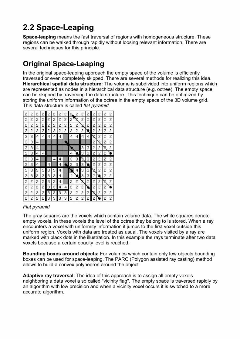
Original Space-LeapingIn the original space-leaping approach the empty space of the volume is efficientlytraversed or even completely skipped. There are several methods for realizing this idea.Hierarchical spatial data structure: The volume is subdivided into uniform regions whichare represented as nodes in a hierarchical data structure (e.g. octree). The empty spacecan be skipped by traversing the data structure. This technique can be optimized bystoring the uniform information of the octree in the empty space of the 3D volume grid.This data structure is called flat pyramid.

Flat pyramidThe image shows an example for a flat pyramid. In fact it is a quadtree recursively subdevided down until pixel size.

The gray squares are the voxels which contain volume data. The white squares denoteempty voxels. In these voxels the level of the octree they belong to is stored. When a rayencounters a voxel with uniformity information it jumps to the first voxel outside thisuniform region. Voxels with data are treated as usual. The voxels visited by a ray aremarked with black dots in the illustration. In this example the rays terminate after two datavoxels because a certain opacity level is reached.

Bounding boxes around objects: For volumes which contain only few objects boundingboxes can be used for space-leaping. The PARC (Polygon assisted ray casting) methodallows to build a convex polyhedron around the object.

Adaptive ray traversal: The idea of this approach is to assign all empty voxelsneighboring a data voxel a so called "vicinity flag". The empty space is traversed rapidly byan algorithm with low precision and when a vicinity voxel occurs it is switched to a moreaccurate algorithm.

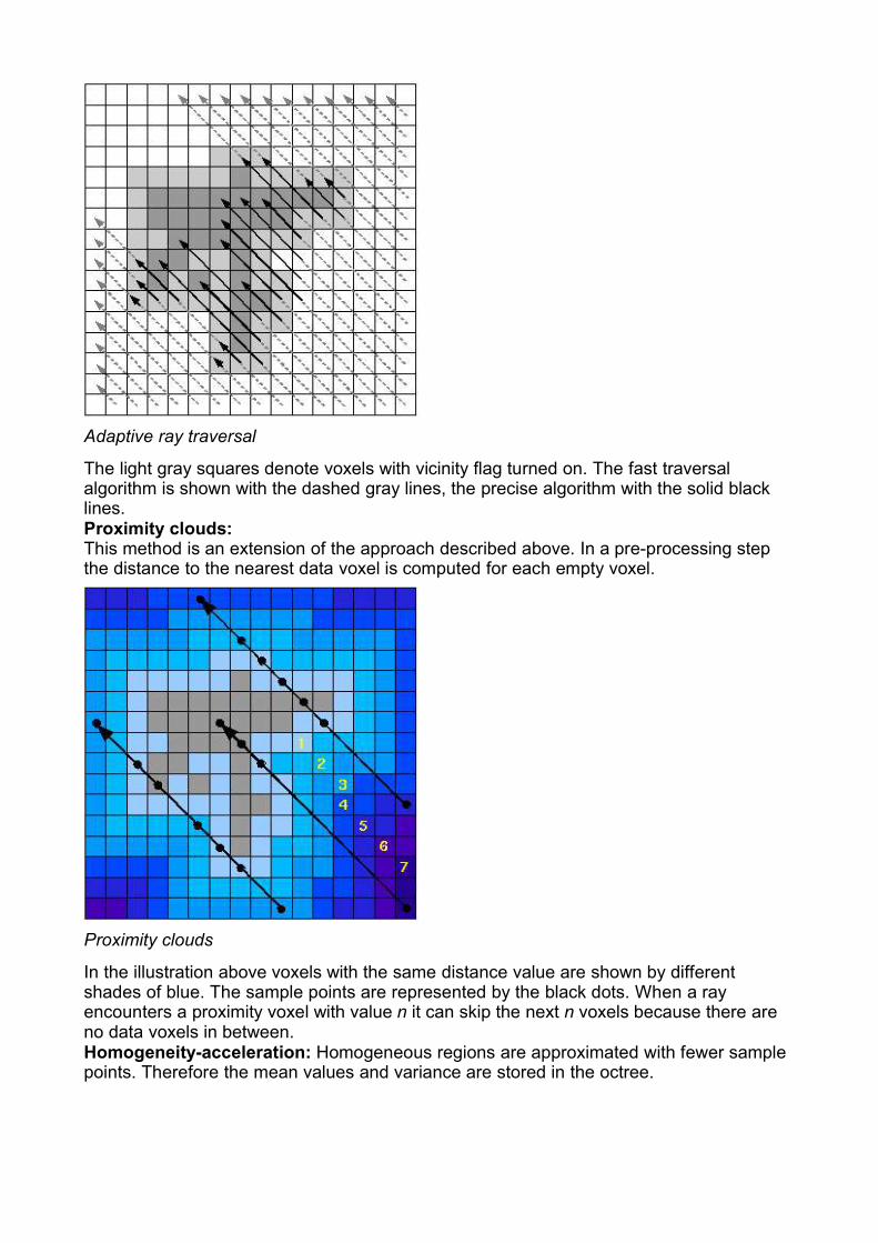
Adaptive ray traversalThe illustration shows an example for adaptive ray traversal

The light gray squares denote voxels with vicinity flag turned on. The fast traversalalgorithm is shown with the dashed gray lines, the precise algorithm with the solid blacklines.Proximity clouds:This method is an extension of the approach described above. In a pre-processing stepthe distance to the nearest data voxel is computed for each empty voxel.

Proximity cloudsThe picture shows an example for proximity clouds.

In the illustration above voxels with the same distance value are shown by differentshades of blue. The sample points are represented by the black dots. When a rayencounters a proximity voxel with value n it can skip the next n voxels because there areno data voxels in between.Homogeneity-acceleration: Homogeneous regions are approximated with fewer samplepoints. Therefore the mean values and variance are stored in the octree.

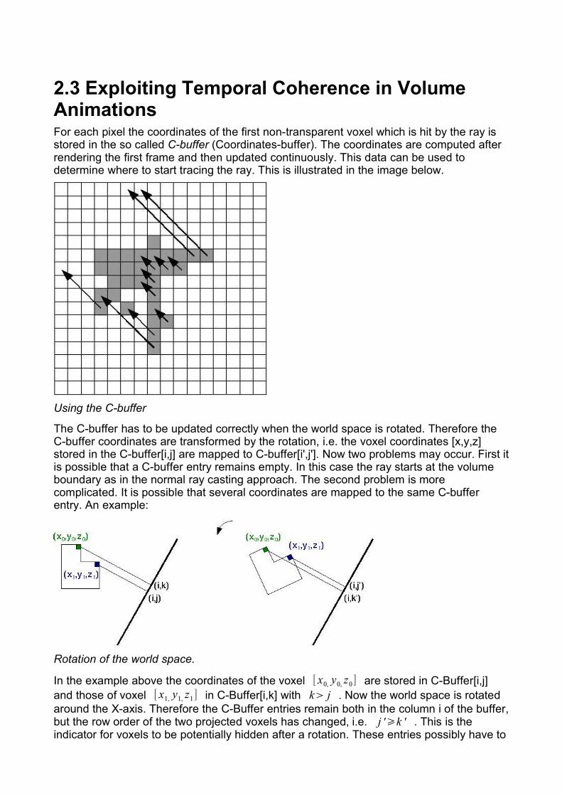
2.3 Exploiting Temporal Coherence in VolumeAnimationsFor each pixel the coordinates of the first non-transparent voxel which is hit by the ray isstored in the so called C-buffer (Coordinates-buffer). The coordinates are computed afterrendering the first frame and then updated continuously. This data can be used todetermine where to start tracing the ray. This is illustrated in the image below.

Using the C-bufferThe image shows an example using the C-buffer.

The C-buffer has to be updated correctly when the world space is rotated. Therefore theC-buffer coordinates are transformed by the rotation, i.e. the voxel coordinates [x,y,z]stored in the C-buffer[i,j] are mapped to C-buffer[i',j']. Now two problems may occur. First itis possible that a C-buffer entry remains empty. In this case the ray starts at the volumeboundary as in the normal ray casting approach. The second problem is morecomplicated. It is possible that several coordinates are mapped to the same C-bufferentry. An example:

Rotation of the world space.The picture shows that after a rotation of the world space points may be hidden.

In the example above the coordinates of the voxel [ x0, y0, z0] are stored in C-Buffer[i,j]and those of voxel [ x1, y1, z1] in C-Buffer[i,k] with k j . Now the world space is rotatedaround the X-axis. Therefore the C-Buffer entries remain both in the column i of the buffer,but the row order of the two projected voxels has changed, i.e. j 'k ' . This is theindicator for voxels to be potentially hidden after a rotation. These entries possibly have to

be removed.

2.4 Template-Based Volume ViewingThe Template-Based Volume Viewing approach by Yagel [Yagel-1992-DRT] stores thetraversal steps through the volume as a ray template to accelerate the rendering process.The template is generated by 3D DDA algorithm and can be used for parallel rays(orthographic projection). The rays have to be traced from a base plane which is orientedparallel to the volume.

Template based volume viewingThe illustration shows an example for template-based volume viewing.

2.5 Adaptive screen samplingIn some applications, rendering is performed by adaptively switching from one renderingmethod or sampling rate to another. Adaptive screen sampling introduced by Levoy[Levoy-1990-HRT] is well known in traditional ray tracing, where the number of raysemitted from a given pixel is adapted to the color change in a subset of pixels in a smallneighborhood. This means that in areas with high value gradients additional rays aretraced. One problem is that the rays occasionally miss the surface, in that case missingvalues are interpolated.

Adaptive screen sampling.In this example we have an area of change from black to white, and therefore high value gradients. In this case adaptive screen sampling switches to a higher sampling rate toreplace interpolated values with exact color values resulting from the second sampling step.

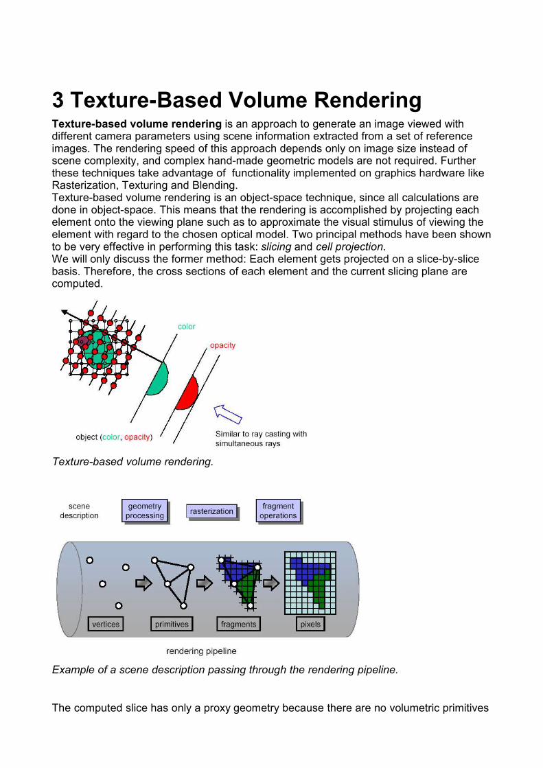
3 Texture-Based Volume RenderingTexture-based volume rendering is an approach to generate an image viewed withdifferent camera parameters using scene information extracted from a set of referenceimages. The rendering speed of this approach depends only on image size instead ofscene complexity, and complex hand-made geometric models are not required. Furtherthese techniques take advantage of functionality implemented on graphics hardware likeRasterization, Texturing and Blending.Texture-based volume rendering is an object-space technique, since all calculations aredone in object-space. This means that the rendering is accomplished by projecting eachelement onto the viewing plane such as to approximate the visual stimulus of viewing theelement with regard to the chosen optical model. Two principal methods have been shownto be very effective in performing this task: slicing and cell projection.We will only discuss the former method: Each element gets projected on a slice-by-slicebasis. Therefore, the cross sections of each element and the current slicing plane arecomputed.

Texture-based volume rendering.At each intersection point with one of the element edges (red points) the color value is interpolatedfrom the pre-shaded samples at cell vertices. The cross sections are then rendered by letting the graphics hardware resample the color values onto the discrete pixel buffer duringrasterization.

Example of a scene description passing through the rendering pipeline.The computation of the sectional polygons can either be done by taking advantage ofdedicated graphics hardware providing per-fragment tests and operations.The computed slice has only a proxy geometry because there are no volumetric primitives

in graphics hardware. By sending the computed vertices of each slice down the renderingpipeline, geometric primitives are generated that get fragmented in the rasterization stepto finally result in a pixel based texture map. All texture-mapped slices are stored in astack and are blended back-to-front onto the image plane, which results in a semi-transparent view of the volume.

This image illustrates a stack of 2D textured slices and the proxy geometry that could beachieved with it.This picture shows a cube drawn only with outlines. Inside the cube there are several slices of a human head blended over each other from back to front.

The texture mapped 2D slices are object-aligned, because they get computed in objectspace parallel to the x-, y-, z-axis, unappreciated from which angle the viewer looks at theobject. Due to correct visualization of the object from each possible viewing angle threestacks of 2D texture slices have to be computed. By doing this one can switch betweenthe different stacks in case the viewing angle is close to 45 degrees to the slice normal.Otherwise the viewer would look on the slice edges and thus see through the volume. Byprojecting the voxels of the slice plane on pixels of the viewing plane, a pixel can lie in-between voxels, so its value can be found by bilinear interpolation.

Axis aligned 2D textured slices.The slices inside the cube are alligned at either the x-, y-, or z-axis.

Another method is to compute view-aligned 3D textured slices. In contrast to the objectaligned method, these slices are arranged with their surface normals in direction of theviewer. Here we only have to compute one stack of 3D textures, but for projection trilinearinterpolation is needed to calculate values in-between. Further, if the object is rotated theslices have to be recomputed for each frame.

View aligned 3D textured slices .The slices in this cube are not aligned at an axis but at the viewpoint. This leads to polyeders that lie parallel to each other.

Example for a teddy bear once rendered with axis aligned slices and once rendered with view aligned slices.

Positive attributes of 2D textures:• This method works on older graphics hardware which does not support 3D textures• Only bilinear interpolation within slices, no trilinear interpolation

• fast• problems with image quality

Problems: • Euclidean distance between slices along a light ray depends on viewing parameters

• sampling distance depends on viewing direction• apparent brightness changes if opacity is not corrected

• Artifacts when stack is viewed close to 45 degrees

Change of brightness in 2D texture-based rendering.A human head rendered 2 times with axis aligned slices from different viewpoints. In the second image the viewpoint is changed in a way, so that more slices lie on top of each

other, this leads to a lucency of the whole head.

Artifacts when stack is viewed close to 45 degrees.The viewpoint points directly on one lateral edge of the cube, which results in visible artefacts. The slices are axis aligned.

Positive attributes of 3D textures:• Needs graphics hardware support for 3D textures• Trilinear interpolation within volume

• slower• good image quality

• Constant Euclidean distance between slices along a light ray• No artifacts due to inappropriate viewing angles

Render components• Data setup

• Volume data representation• Transfer function representation

• Data download• Volume textures• Transfer function tables

• Per-volume setup (once per frame)• Blending mode configuration• Texture unit configuration (3D)• (Fragment shader configuration)

• Per-slice setup• Texture unit configuration (2D)• Generate fragments• Proxy geometry rendering

Representation of volume data by textures:• Stack of 2D textures• One 3D texture

Typical choices for texture format:• Luminance and alpha

• Pre-classified (pre-shaded) gray-scale volume rendering• Transfer function is already applied to scalar data• Change of transfer function requires complete redefinition of texture data

• RGBA• Pre-classified (pre-shaded) colored volume rendering• Transfer function is already applied to scalar data

• Paletted texture• Index into color and opacity table (= palette)• Index size = byte• Index is identical to scalar value• Pre-classified (pre-shaded) colored volume rendering

• Transfer function applied to scalar data during runtime• Simple and fast change of transfer functions• OpenGL code for paletted 3D textureglTexImage3D ( GL_TEXURE_3D, 0, GL_COLOR_INDEX8_EXT,

size_x, size_y, GL_COLOR_INDEX, GL_UNSIGNED_BYTE, voldata);

• Representation of transfer function:• For paletted texture only• 1D transfer function texture = lookup table• OpenGL extensions required• OpenGL codeglColorTableEXT (GL_SHARED_TEXTURE_PALETTE_EXT,

GL_RGBA8, 256*4, GL_RGBA,GL_UNSIGNED_BYTE, palette);

Compositing:• Works on fragments• Per-fragment operations• After rasterization• Blending of fragments via over operator• OpenGL code for over operator

glEnable (GL_BLEND);glBlendFunc (GL_SRC_ALPHA, GL_ONE_MINUS_SRC_ALPHA);

Generate fragments:• Render proxy geometry• Slice• Simple implementation: quadrilateral• More sophisticated: triangulated intersection surface between slice plane and boundary

of the volume data set

Advantages of texture-based rendering:• Supported by consumer graphics hardware• Fast for moderately sized data sets• Interactive explorations• Surface-based and volumetric representations can easily be combined

• mixture with opaque geometries

Disadvantages of texture-based rendering:• Limited by texture memory

• Solution: bricking at the cost of additional texture downloads to the graphicsboard

• Brute force: complete volume is represented by slices• No acceleration techniques like early-ray termination or space leaping• Rasterization speed and memory access can be problematic

Outlook on more advanced texture-based volume rendering techniques:• Exploit quite flexible per-fragment operations on modern GPUs (nVidia GeForce 3/4 or

ATI Radeon 8500)• Post-classification (post-shading) possible• So-called pre-integration for very high-quality rendering• Decompression of compressed volumetric data sets on GPU to save texture memory

• Object-space method• Slice-based technique• Fast object-order rendering• Accelerated volume visualization via shear-warp factorization [Lacroute & Levoy 1994]• Software-based implementation

4 Shear-Warp FactorizationAs described in the last chapter, algorithms that use spatial data structures can be dividedinto two categories according to the order in which the data structures are traversed:image-order or object-order. Image-order algorithms operate by casting rays from each image pixel and processing thevoxels along each ray (e.g. Ray Casting). This processing order has the disadvantage thatthe spatial data structure must be traversed once for every ray, resulting in redundantcomputation (e.g. Multiple descents of an octree). In contrast, object-order algorithmsoperate by splatting voxels onto the image while streaming through the volume data instorage order. We will deal with this technique more deeply in this chapter. However, thisprocessing order makes it difficult to implement early ray termination, an effectiveoptimization in ray-casting algorithms.

Lacroute [Lacroute-1994-FVR] presented an accelerated volume visualization algorithmvia Shear-Warp factorization that combines the advantages of image-order and object-order algorithms.

The algorithm is software-based and works on the same slice-based technique as texturebased volume rendering. Therefore it also needs 3 stacks of the volume along 3 principalaxes. They are computed in object-space. The general goal is to make viewing raysparallel to each other and perpendicular to the image, which is achieved by a simpleshear.

Shear along the volume slices.This figure illustrates the transformation from object space to sheared object space for a parallel projection. The horizontal lines in the figure represent slices of the volume dataviewed in cross-section. After transformation the volume data has been sheared parallel to the set of slices that is most perpendicular to the viewing direction and the viewing raysare perpendicular to the slices.

Mathematical description of the shear-warp factorization:Splitting the viewing transformation into separate partsM view=P⋅S⋅M warp

where M view = general viewing matrixP = permutation matrix: transpose the coordinate system in order to make the z-

axis the principal viewing axis. (Note that P stands not for the Projection)S = transforms volume into sheared object spaceM warp =warps sheared object coordinates into image coordinates

Shear S for parallel and perspective projections:

S par=1 0 sx 00 1 s y 00 0 1 00 0 0 1

S persp=1 0 s ' x 00 1 s ' y 00 0 1 00 0 s ' w 1

Algorithm:1. Transform the volume data to sheared object space by translatingand resampling each slice according to S . For perspectivetransformations, also scale each slice. P specifies which ofthe three possible slicing directions to use. For resamplingbilinear interpolation is used.

2. Composite the resampled slices together in front-to-back orderusing the over operator. This step projects the volume into a 2Dintermediate image in sheared object space. Here we can useearly ray termination to accelerate the algorithm.

3. Transform the intermediate image to image space by warping itaccording to M warp This second resampling step produces thecorrect final image.

Shear along the volume slices, composite the resampled slices to an intermediate imageand warp it to image space.In this illustration, several parallel rays are cast through the volume slices in any angle. In the second step, all rays are sheared at the first slice, so they stand perpendicular on it.

Example for one scan line:

After shearing slices, you have to resample them. Then the sample ray hits voxel center

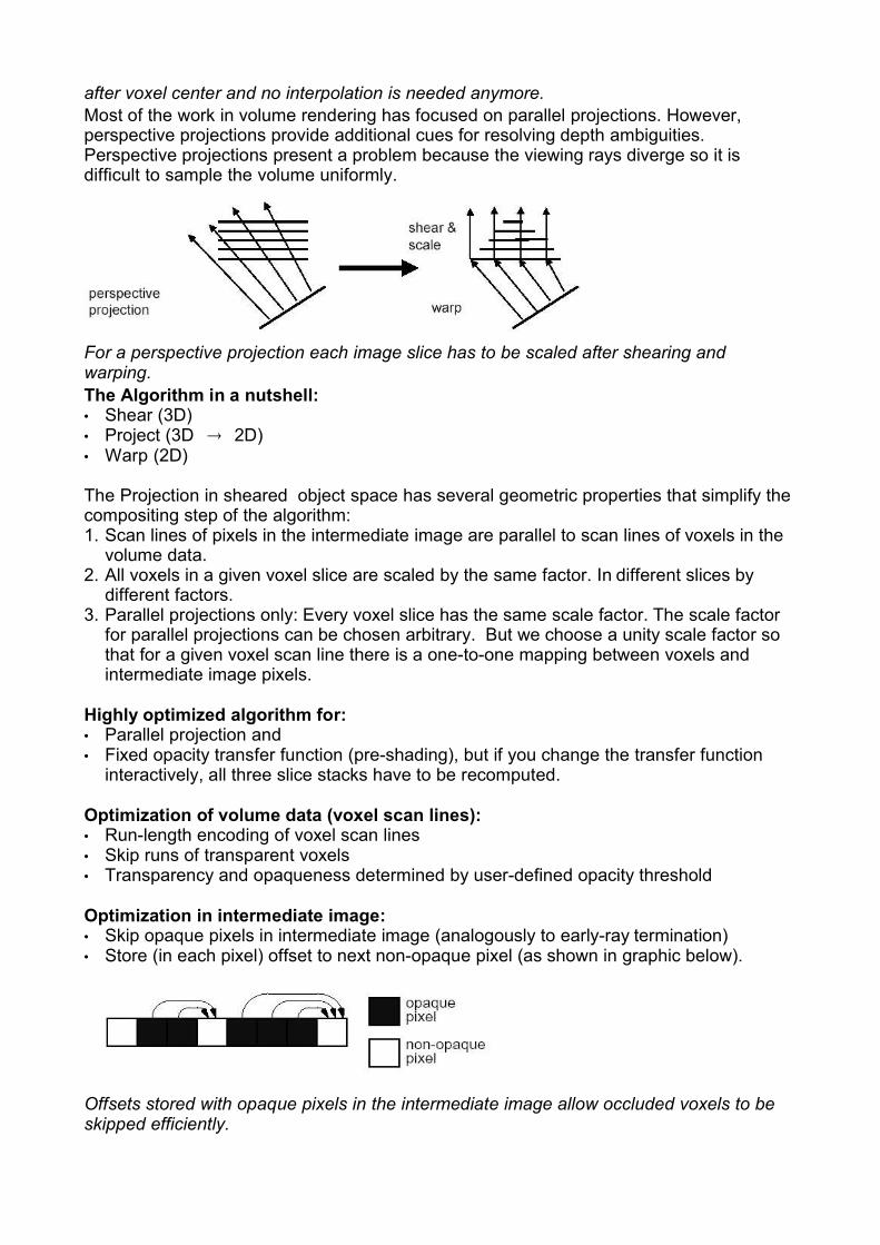
after voxel center and no interpolation is needed anymore.Most of the work in volume rendering has focused on parallel projections. However,perspective projections provide additional cues for resolving depth ambiguities.Perspective projections present a problem because the viewing rays diverge so it isdifficult to sample the volume uniformly.

For a perspective projection each image slice has to be scaled after shearing andwarping.The Algorithm in a nutshell:• Shear (3D)• Project (3D 2D)• Warp (2D)

The Projection in sheared object space has several geometric properties that simplify thecompositing step of the algorithm:1. Scan lines of pixels in the intermediate image are parallel to scan lines of voxels in the

volume data.2. All voxels in a given voxel slice are scaled by the same factor. In different slices by

different factors.3. Parallel projections only: Every voxel slice has the same scale factor. The scale factor

for parallel projections can be chosen arbitrary. But we choose a unity scale factor sothat for a given voxel scan line there is a one-to-one mapping between voxels andintermediate image pixels.

Highly optimized algorithm for:• Parallel projection and• Fixed opacity transfer function (pre-shading), but if you change the transfer function

interactively, all three slice stacks have to be recomputed.

Optimization of volume data (voxel scan lines):• Run-length encoding of voxel scan lines• Skip runs of transparent voxels• Transparency and opaqueness determined by user-defined opacity threshold

Optimization in intermediate image:• Skip opaque pixels in intermediate image (analogously to early-ray termination)• Store (in each pixel) offset to next non-opaque pixel (as shown in graphic below).

Offsets stored with opaque pixels in the intermediate image allow occluded voxels to beskipped efficiently.This picture shows a row of 8 pixels. Pixel 1, 4 and 8 are non-opque (white), the others are opaque (black). Each opaque pixel has a pointer stored, that points to the next non-opaque pixel.

By combining the both ideas of volume data and intermediate image optimization, we canexploit coherencies and make the algorithm very fast. As first property parallel scan linesare used for pixels and voxels. That means that voxel scan lines in sheared volume arealigned with pixel scan lines in intermediate image and both can be traversed in scan lineorder simultaneously. By using the run-length encoding of the voxel data to skip voxelswhich are transparent and the run-length encoding of the image to skip voxels which areoccluded, we perform work only for voxels which are both non-transparent and visible.

Resampling and compositing are performed by streaming through both the voxels and theintermediate image in scanline order, skipping over voxels which are transparent andpixels which are opaque.Coherence in voxel space:• Each slice of the volume is only translated• Fixed weights for bilinear interpolation within voxel slices• Computation of weights only once per frame

Final warping:• Works on composited intermediate image• Warp: affine image warper with bilinear filter• Often done in hardware: render a quadrilateral with intermediate 2D image being

attached as 2D texture

Parallel projection:• Efficient reconstruction• Lookup table for shading• Lookup table for opacity correction (thickness)• Three RLE of the actual volume (in x, y, z)

Perspective projection:• Similar to parallel projection• Viewing rays diverge in infinity• Difference: voxels need to be scaled• Hence more then two voxel scan lines needed for one image scan line• Many-to-one mapping from voxels to pixels makes it slower than parallel projection.

5 SplattingSplattingSplatting is a volume rendering method that distributes volume data values across aregion on the rendered image in terms of a distribution function.

Splatting is an object-order method described by [Westover, 1990], this methodaccumulates data points by "throwing" kernels for each voxel to the drawing plane. Thefootprints on the drawing plane represent the visualization. The kernel shape and size iscritical for the quality of the result. The accumulation, or compositing process can be doneback-to-front, which guarantees correct visibility. Front-to-back compositing is faster,because the process can be stopped when pixels are fully opaque. The original algorithmis fast but poor in quality, however since the first publication many improvements havebeen implemented. Note that good splatting results need as much CPU computing time asray casting.

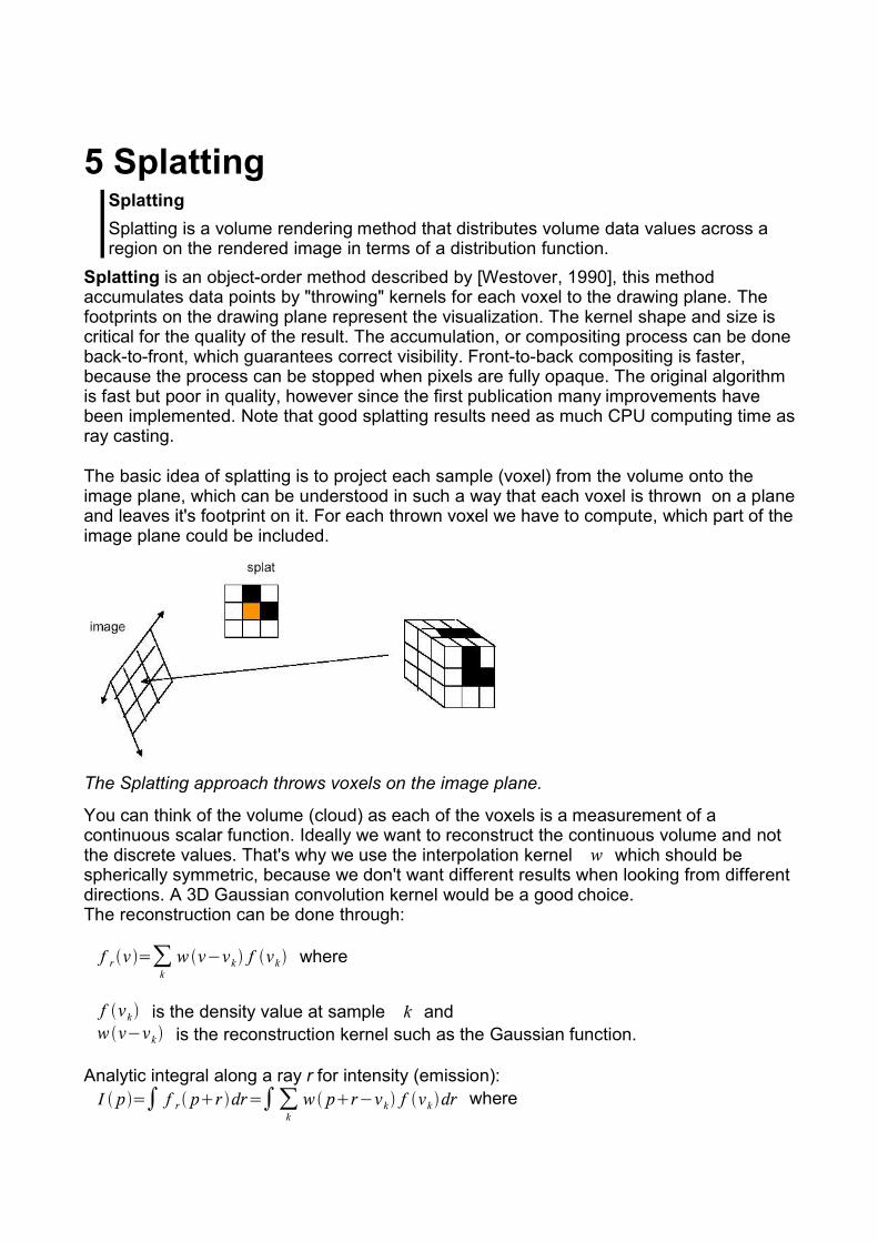
The basic idea of splatting is to project each sample (voxel) from the volume onto theimage plane, which can be understood in such a way that each voxel is thrown on a planeand leaves it's footprint on it. For each thrown voxel we have to compute, which part of theimage plane could be included.

The Splatting approach throws voxels on the image plane.Illustrated is a 3D cube with 3 on 3 on 3 cells that throws its voxels on a 2D plane 3 on 3 pixels. Each voxel leaves a splat on the image plane.

You can think of the volume (cloud) as each of the voxels is a measurement of acontinuous scalar function. Ideally we want to reconstruct the continuous volume and notthe discrete values. That's why we use the interpolation kernel w which should bespherically symmetric, because we don't want different results when looking from differentdirections. A 3D Gaussian convolution kernel would be a good choice.The reconstruction can be done through:

f r v =∑kw v−vk f vk where

f vk is the density value at sample k andw v−vk is the reconstruction kernel such as the Gaussian function.

Analytic integral along a ray r for intensity (emission):I p=∫ f r pr dr=∫∑

kw pr−vk f vk dr where

I p is the intensity for pixel p,f r is the scale intensity,r is the ray and ∑k is the sum of all voxels weighted by the kernel.

We can rewrite the formula by switching the summation and integral:I p=∑

kf vk ⋅∫w pr−vk dr

with ∫w pr−vk dr as splatting kernel (= “splat”) or footprint.

Discretization via 2D splats, where ray is in z-axis:Splat x , y =∫w x , y , z dz

from the original 3D kernel. Often w is chosen as Gaussianw x , y , z =d exp −x2/a2− y2/b2−z2/c2

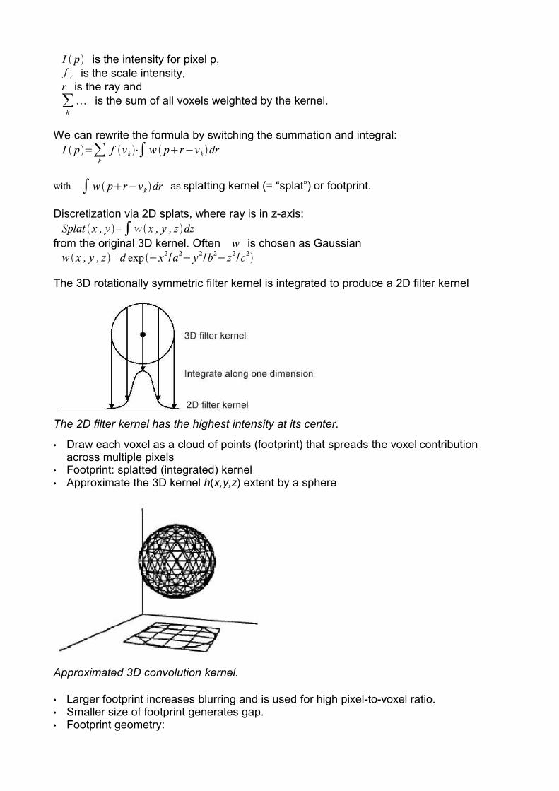
The 3D rotationally symmetric filter kernel is integrated to produce a 2D filter kernel

The 2D filter kernel has the highest intensity at its center.A crop of the 3D gaussian kernel filter looks like a circle. The integration in one dimension gives us the typical symetric 2D gaussian kernel filter that looks like a hat.

• Draw each voxel as a cloud of points (footprint) that spreads the voxel contributionacross multiple pixels

• Footprint: splatted (integrated) kernel• Approximate the 3D kernel h(x,y,z) extent by a sphere

Approximated 3D convolution kernel.This image shows the 3D gaussian filter kernel that looks like a sphere.• Larger footprint increases blurring and is used for high pixel-to-voxel ratio.• Smaller size of footprint generates gap.• Footprint geometry:

• Orthographic projection: footprint is independent of the view point.• Perspective projection: footprint is elliptical.

• The splat footprint, a function of x and y can be pre-computed and stored. Oncethis is done, the algorithm just needs to add many of the footprints for projection onimage plane.

• For perspective projection: additional computation of the orientation of the ellipse.

2D convolution kernel.If the 3D spheric kernel gets projected on a 2D plane by a pespective projection it leavesan elliptical footprint.The choice of kernel can affect the quality of the image as you can see in the picturebelow. Examples are cone, Gaussian, sinc, and bilinear function.

Example of the 2D Gaussian convolution kernel.For splatting, each slice of the volume is filled with a field of 3D interpolation kernels, onekernel at each grid voxel. The reconstruction kernels might overlap and each of themleaves a 2D footprint on the screen, which is weighted and accumulated into the finalimage.

Splatts on the viewing plane.This image shows 2 overlapping splats on the viewing plane. The footprints on the screen are accumulated by the color of botch splats.

Voxel kernels are added within each 2D sheet of the volume. The weighted footprints ofthe sheets are composited in front-to-back order. For projection of all sheets in the sheet-buffer we use volume slices most parallel to the image plane (analogously to stack ofslices).

Which stack of volume slices is used for projection onto the image plane depends of theviewing angle.If the viewing angle is about 30 degrees we choose the stack aligned at the x-axis, if theangle is about 70 degrees we choose the stack aligned at the y-axis.Core algorithm for splatting:Volume:• Represented by voxels• SlicingImage plane:• Sheet buffer• Compositing buffer

Add voxel kernels within first sheet to the sheet-buffer.

Transfer sheet buffer to compositing buffer.

Add voxel kernels within second sheet to the sheet-buffer.

Composite sheet buffer with compositing buffer.

Add voxel kernels within third sheet to the sheet-buffer

Composite sheet buffer with compositing buffer.A problem that leads to inaccurate compositing is when two or more splats overlap. Inthese regions we will have an incorrect mixture of integration (3D kernel to 2D splat) andcompositing.

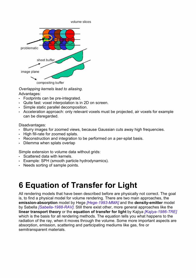
Overlapping kernels lead to aliasing.Advantages:• Footprints can be pre-integrated.• Quite fast: voxel interpolation is in 2D on screen.• Simple static parallel decomposition.• Acceleration approach: only relevant voxels must be projected, air voxels for example

can be disregarded.

Disadvantages:• Blurry images for zoomed views, because Gaussian cuts away high frequencies.• High fill-rate for zoomed splats.• Reconstruction and integration to be performed on a per-splat basis.• Dilemma when splats overlap

Simple extension to volume data without grids:• Scattered data with kernels.• Example: SPH (smooth particle hydrodynamics).• Needs sorting of sample points.

6 Equation of Transfer for LightAll rendering models that have been described before are physically not correct. The goalis, to find a physical model for volume rendering. There are two main approaches, theemission-absorption model by Hege [Hege-1993-MMA] and the density-emitter modelby Sabella [Sabella-1988-RAV]. Still there exist other, more general approaches like thelinear transport theory or the equation of transfer for light by Kajiya [Kajiya-1986-TRE]which is the basis for all rendering methods. The equation tells you what happens to theradiation of the ray, when it moves through the volume. Some more important aspects areabsorption, emission, scattering and participating mediums like gas, fire orsemitransparent materials.

Two ways to make the equation of transfer simpler:1. Changes can only appear by interaction with surfaces, if there is no medium (vacuum)

it does not effect the ray and we can use the standard rendering equation. Theradiance resides constant.

2. If there is a medium, we have absorbtion along the ray passing through the volume. Buttherefore with the emission-absorbtion model we have no scattering, which means nochange of direction and no computation of secundary rays. In this case we can use thestandard volume rendering equation.

Based on the geometric optics, we select the equation of transfer dependant on themedium or depandant on scattering. If there is no medium we can choose the standardrendering equation or more precise the radiosity equation. And if there is no scattering wecan choose the typical volume rendering equation.The basic idea of the equation of transfer for light is very much in the spirit of the radiosityequation, simply balancing the energy flows from one point of a surface to another. Theequation states that the transport intensity of light from one surface point to another issimply the sum of the emitted light and the total light intensity which is scattered towardx from all other surface points. Further on, the more detailed explanations are based

on the equation model by Hege [Hege-1993-MMA] .

Assumptions:• Based on a physical model for radiation• Geometrical optics

Neglect:• Diffraction• Interference• Wave-character• Polarization

Interaction of light with matter at the macroscopic scale:• Describes the changes of specific intensity due to absorption, emission, and scattering

Based on energy conservation on microscopic level (not on photon and electron level).

• Basic quantity of light is the radiance, sometimes also called specific intensity I .

Photons reflected on a surface.Given is a round surface with surface area dA , a reflection vector n with angle to the surface normal and the solid

angle d .

The equation of radiative energy tells us, if we have a surface element and radiation withspecific direction n with solid angle, what the amount of energy moving through thisarea will be. Therefore the equation looks like:

E= I x ,n , v cos dA d d dt with

E = amount of radiation energy, traveling in time dt with a frequency intervald around through a surface element dA into an element of solid angle d in

direction n .I = radiance or specific intensity (6 dimensional: position: 2 dimensions (angles),

direction: 3 dimensions, frequency: 1 dimension).x = positionn = directionv = frequency = angle between n and the normal on dAcos dA = projected area elementd = solid angled = frequencydt = time

There exist 4 responsible effects if there is a difference between incoming and outgoingradiance at a single position:• Absorption: specific intensity comes in, less intensity goes out.• Emission: less energy comes in, but more energy goes out.• Outscattering: energy scatters out in all directions and can scatter in at another part.• Inscattering: energy scatters in from other parts.

Contributions to radiation at a single position.This illustration shows the 4 different contributions to radiation. If it comes to absorbtion, more energy goes into one point than comes out again. Outscattering distributes theincoming energy in all directions. Emission at one point sets more energy free, as incoming energy. Inscattering collects energy from every direction and sets it free in one specificdirection.

Absorption:When radiation passes through material, energy is generally removed from the beam. Thisloss is described in terms of an extinction coefficient or total absorption coefficientx ,n , v .

The amount of energy removed from a beam with specific intensity I x ,n , , whenpassing through a cylindrical volume element of length ds and cross section da , isgiven by:

Eab=x ,n , v I x ,n , v ds dA d dv dt with

Eab = absorptionx ,n , = absorption coefficient = scalar value or function

Notice that no cosine term appears in this expression. This is because the absorbingvolume does not depend on the incident angle. The absorption coefficient generally is afunction of x , n and z . The absorption coefficient is measured in units of m−1 .

The term 1 is also known as the mean free path of photons of frequency in

material.

Removal of radiative energy by true absorption (conversion to thermal energy).Absorption of energy through a cylindrical volume element is proportional to its length.

It is important to distinguish between true or thermal absorption and emission processes,and the process of scattering. In the former case, energy removed from the beam isconverted into material thermal energy, and energy is emitted into the beam at theexpense of material energy respectively. In contrast, in a scattering process a photoninteracts with a scattering center and emerges from the event moving in a differentdirection, in general with a different frequency too. Therefore the total absorptioncoefficient consists of two parts:• True absorption coefficient x ,n ,• Scattering coefficient x ,n ,

total absorption coefficient; =The ratio of scattering coefficient and total absorption coefficients albedo. An albedo of 1means, that there will be no true absorption at all. This is the case of perfect scattering.

Scattering out of solid angle d .Emission:The emission coefficient x ,n , is defined in such a way, that the amount of radiant

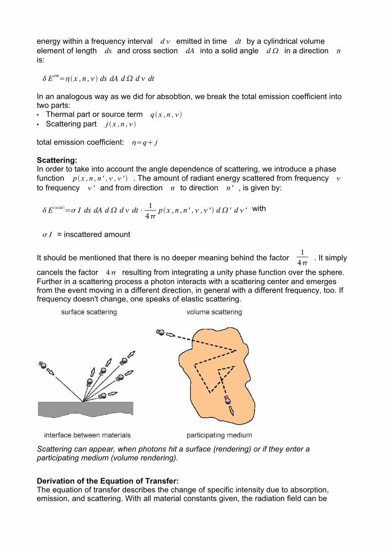
energy within a frequency interval d emitted in time dt by a cylindrical volumeelement of length ds and cross section dA into a solid angle d in a direction nis:

Eem= x ,n , ds dA d d dt

In an analogous way as we did for absobtion, we break the total emission coefficient intotwo parts:• Thermal part or source term q x ,n ,• Scattering part j x ,n ,

total emission coefficient: =q j

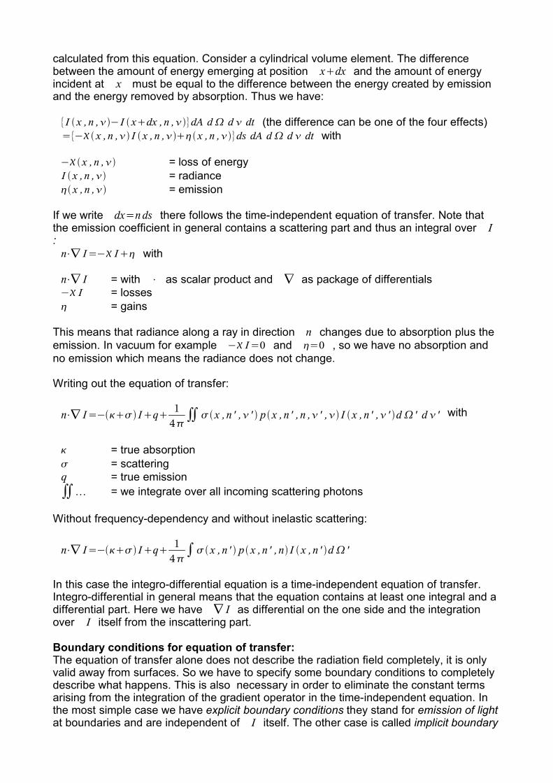
Scattering:In order to take into account the angle dependence of scattering, we introduce a phasefunction p x ,n ,n ' , , ' . The amount of radiant energy scattered from frequency to frequency ' and from direction n to direction n ' , is given by:

Escat = I ds dA d d dt⋅ 14

p x ,n ,n ' , , ' d ' d ' with

I = inscattered amount

It should be mentioned that there is no deeper meaning behind the factor 1

4 . It simply

cancels the factor 4 resulting from integrating a unity phase function over the sphere.Further in a scattering process a photon interacts with a scattering center and emergesfrom the event moving in a different direction, in general with a different frequency, too. Iffrequency doesn't change, one speaks of elastic scattering.

Scattering can appear, when photons hit a surface (rendering) or if they enter aparticipating medium (volume rendering).This picture shows an example of surface scattering. Incoming energy from one specific direction scatteres on the surface and gets distributed in several directions. The nextexample shows volume scattering inside a medium. There the incoming energy gets scattered several times inside the medium, which always results in a change of the reflectionangle. This means the energy can enter the medium at any point and can leave it at any other possible point, depending on how often it scatters.

Derivation of the Equation of Transfer:The equation of transfer describes the change of specific intensity due to absorption,emission, and scattering. With all material constants given, the radiation field can be

calculated from this equation. Consider a cylindrical volume element. The differencebetween the amount of energy emerging at position xdx and the amount of energyincident at x must be equal to the difference between the energy created by emissionand the energy removed by absorption. Thus we have:

{I x ,n ,− I xdx ,n ,}dA d d dt (the difference can be one of the four effects)={− x ,n , I x ,n ,x ,n ,}ds dA d d dt with

−x ,n , = loss of energyI x ,n , = radiance x ,n , = emission

If we write dx=nds there follows the time-independent equation of transfer. Note thatthe emission coefficient in general contains a scattering part and thus an integral over I:n⋅∇ I=− I with

n⋅∇ I = with ⋅ as scalar product and ∇ as package of differentials− I = losses = gains

This means that radiance along a ray in direction n changes due to absorption plus theemission. In vacuum for example − I=0 and =0 , so we have no absorption andno emission which means the radiance does not change.

Writing out the equation of transfer:

n⋅∇ I=− Iq 14∬x ,n ' , ' p x ,n ' ,n , ' , I x ,n ' , ' d ' d ' with

= true absorption = scatteringq = true emission∬ = we integrate over all incoming scattering photons

Without frequency-dependency and without inelastic scattering:

n⋅∇ I=− Iq 14∫x ,n ' p x ,n ' ,n I x ,n ' d '

In this case the integro-differential equation is a time-independent equation of transfer.Integro-differential in general means that the equation contains at least one integral and adifferential part. Here we have ∇ I as differential on the one side and the integrationover I itself from the inscattering part.

Boundary conditions for equation of transfer:The equation of transfer alone does not describe the radiation field completely, it is onlyvalid away from surfaces. So we have to specify some boundary conditions to completelydescribe what happens. This is also necessary in order to eliminate the constant termsarising from the integration of the gradient operator in the time-independent equation. Inthe most simple case we have explicit boundary conditions they stand for emission of lightat boundaries and are independent of I itself. The other case is called implicit boundary

condition and stands for reflection of light at surfaces. A combination of explicit andimplicit boundary conditions on boundary surface can be written:

I x ,n ,=E x ,n ,∬ k x ,n ' ,n , ' , I incx ,n ' , ' d ' d ' with

E x ,n , = emission∬ k x ,n ' , n , ' , = surface scattering kernelI inc x ,n ' , ' = incoming radiation

Integral form of the Equation of Transfer:Instead of an integro-differential equation we can rewrite the equation of transfer to a pureintegral equation:

n⋅∇ I x ,n ,=−x ,n , I x ,n ,x ,n ,

yields

∂∂ sI x ,n ,=−x ,n , I x ,n ,x ,n ,

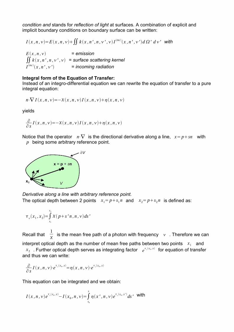
Notice that the operator n⋅∇ is the directional derivative along a line, x= psn withp being some arbitrary reference point.

Derivative along a line with arbitrary reference point.The optical depth between 2 points x1= ps1n and x2= ps2n is defined as:

x1 , x2=∫s1

s2

ps ' n ,n ,ds '

Recall that 1 is the mean free path of a photon with frequency . Therefore we can

interpret optical depth as the number of mean free paths between two points x1 andx2 . Further optical depth serves as integrating factor e x0 , x for equation of transfer

and thus we can write:

∂∂ sI x ,n ,⋅ex0 , x =x ,n ,⋅ex0 , x

This equation can be integrated and we obtain:

I x ,n ,e x0 , x −I x0 , n ,=∫s0

s

x ' ,n ,ex0 , x ' ds ' with

∫s0

s

x ' , n , = integral of total emission

ex0 , x ' = integrating factorx0 = on the boundary surface

Making use of the fact that optical depth can be decomposed intox0 , x = x0 , x ' x ' , x the final integral form of the equation of transfer can be

written as follows:

I x ,n ,=I x0 , n ,e−x0 , x ∫

s0

s

x ' , n ,e−x ' , x ds ' with

I x0 , n ,e−x0 , x = at any point of the volume there can be emission.

∫s0

s

x ' ,n ,e− x ' , x = if there is emission at a point in the volume it will be absorbed on

its further way.

This equation can be viewed as the general formal solution of the time-independentequation of transfer. It states that the intensity of radiation traveling along n at pointx is the sum of photons emitted from all points along the line segment x '= ps ' n ,

attenuated by the integrated absorptivity of the intervening material, plus an attenuatedcontribution from photons entering the boundary surface when it is pierced by that linesegment. Generally the emission coefficient will contain I itself.Vacuum condition is an important special case of the transport equation, because there isno absorption, emission or scattering at all, except on surfaces. Further the frequencydependence can be ignored and the equation of transfer (inside the volume) is greatlysimplified:

I x ,n=I x0 , n

Rays incident on surface at x are traced back to some other surface element at x ' :

I inc x ,n ' =I x ' ,n '

If we substitute this into the generic boundary condition:

I x ,n ,=E x ,n ,∬ k x ,n ' ,n , ' , I incx ,n ' , ' d ' d '

we obtain the famous rendering equation published by Kajiya [Kajiya-1986-TRE]:

I x ,n=E x ,n∫k x ,n ' ,n I inc x ,n ' d ' , x∈S with S = surface

Rewriting the element of solid angle d ' into a more familiar form

d '=cos ' ∣x−x '∣

dA '

leads to the standard form via BRDF (bidirectional reflection distribution function):

k x ,n ' , n= f r x ,n ' ,ncosi

Special case for most volume rendering approaches:• Emission-absorption model• Density-emitter model [Sabella-1988-RAV]• Volume filled with light-emitting particles• Particles described by density function

If we ignore scattering in volume rendering equation we are left with the so calledemission-absorption model or density-emitter model. One can imagine the volume tobe filled with small light emitting particles. Rather than being modeled individually, theseparticles are described by some density function. This leads to some Simplifications:• No scattering• Emission coefficient consists of source term only: =q (true emission)• Absorption coefficient consists of true absorption only: =• No mixing between frequencies (no inelastic effects), so we can ignore any

Let us consider a ray of light traveling along a direction n , parametrized by a variables . The ray enters the volume at position s0 . Suppressing the argument n , the

equation of transfer in integral form reads:

I s=I s0e−s0 , s∫

s0

s

q s ' e−s ' , sds ' with

I s0 = incoming radiance is usually given by the boundary conditions.e−s0 , s = absorptionq s ' = emission insidee−s ' , s = absorption on the way out

with optical depth

s1 , s2=∫s1

s2

sds

This equation is much simpler because we are only interested in the radiance along theray without any scattering. In order to solve this equation one has to discretize along theray. There is no need to use equidistant steps, though this is the most common usedprocedure. If we divide the range of integration into n intervals , then the specificintensity at position sk is related to the specific intensity at position sk−1 by the identity.So the discretization of volume rendering equation can be written:

I sk = I sk−1e−sk−1 , sk ∫

sk−1

sk

q se−s , sk ds with

e−sk−1 , sk = attenuation between sk−1 and skq s = emission term with q , the color which is emitted

For abbreviation we define two parts:

• Transparency part: k=e−sk−1 , sk

• Emission part: bk=∫sk−1

sk

q se−s , sk

So specific intensity at sn can now be written as:

I sn=I sn−1nbn−∑k=0

n

bk ∏j=k1

n

j=I S n−1⋅1−nbn

This formula describes the entire physics of radiation transport, with the sum of all thingsthat get emitted and the product of all transparencies (this is the over operator from raycasting). More exact the quantity k is called the transparency of the material betweensk−1 and sk . Transparency is a number between 0 and 1. An infinitely optical depthsk−1 , sk corresponds to a vanishing transparency k=0 . On the other hand a

vanishing optical depth corresponds to full transparency k=1 . Alternatively one oftenuses opacity, defined as k=1−k .

7 Compositing SchemesAs a matter of course there exist variations of composition schemes other then the overoperator:• First• Average• Maximum intensity projection• Accumulate

Illustration of different styles of compositing schemes.Given is a arbitrarily density function in a coordinate system where the x-axis stands fordepth and the y-axis stands for the intensity. The composite first hit works as follows: Send a ray into a volume, if the scalar value at apoint is higher then the threshold use this one to extract isosurfaces and render them.

For the first value above a specified threshold is used for rendering.First hit renderning leads to a simple solid isosurface of the specified value.

Average or linear compositing produces basically an X-ray picture and takes no opacityinto account.

The result of average compositing looks like an X-ray picture.Average sends a ray through the volume and composits all found values with the same weight.

Maximum Intensity Projection (MIP) uses the greatest value for rendering. It is often usedfor magnetic resonance angiograms or to extract vessel structures from an CT or MRTscan.

MIP emphasises structures with high intensities.Maximum Intensity Projection takes only the highest values into account.

Accumulate compositing is similar to the over operator and the emission-absorption modelwhere we have early ray termination. Intensity colors are accumulated until enoughopacity is collected. This makes transparent layers visible (see volume classification).

Accumulation stops if enough opacity is collected.If one uses accumulation you get a semi-transparent representation of the object.

8 Non-uniform Grids• Resampling approaches, adaptive mesh refinement (AMR)• Cell projection for unstructured (tetrahedral) grids• Shirley-Tuchman [Shirley-1990-PAD]