direct and inverse problems for nonlinear time-harmonic
TRANSCRIPT

IntroductionNonlinear Maxwell’s Equations
Direct and Inverse Problems for NonlinearTime-harmonic Maxwell’s Equations
TING ZHOUNortheastern University
IAS Workshop on Inverse Problems,Imaging and PDE
joint work with Y. Assylbekov
TING ZHOU Northeastern University HKUST

IntroductionNonlinear Maxwell’s Equations
Outline
1 Introduction
2 Nonlinear Maxwell’s EquationsKerr-type NonlinearityConstruction of CGO solutionsContinue the proof for the case of Kerr-type nonlinearitySecond Harmonic Generation (SHG)
TING ZHOU Northeastern University HKUST

IntroductionNonlinear Maxwell’s Equations
Calderón’s Problem
Electrical Impedance Tomography: Recover electric conductivity of anobject from voltage-to-current measurements on the boundary.
Posed by Alberto Calderón (1980).
Voltage-to-current measurements are modeled by theDirichlet-to-Neumann-map
Λσ : f 7→ σ∂νu|∂Ω
where u solves ∇ · (σ∇u) = 0 in Ω, u|∂Ω = f .
Inverse Problem: Determine σ from Λσ .
TING ZHOU Northeastern University HKUST

IntroductionNonlinear Maxwell’s Equations
Inverse Problem for Maxwell’s equations
Consider the time-harmonic Maxwell’s equations with a fixed(non-resonance) frequency ω > 0
∇× E = iωµH and ∇× H = −iωεE in Ω ⊂ R3.
E,H : Ω→ C3 electric and magnetic fields;ε, µ ∈ L∞(Ω;C) electromagnetic parameters with Re(ε) ≥ ε0 > 0 andRe(µ) ≥ µ0 > 0;Electromagnetic measurements on ∂Ω are modeled by the admittancemap
Λε,µ : ν × E|∂Ω 7→ ν × H|∂Ω.
Inverse Problem: Determine ε and µ from Λε,µ.
TING ZHOU Northeastern University HKUST

IntroductionNonlinear Maxwell’s Equations
Uniquness Results
Conductivity equation:Calderón (1980) for the linearized inverse problem;Kohn-Vogelius (1985) for piecewise real-analytic conductivities;Sylvester-Uhlmann (1987) for smooth conductivities (n ≥ 3);Nachman (1996) for n = 2;
Maxwell’s equations:Somersalo-Isaacson-Cheney (1992) for the linearized inverse problem;Ola-Päivärinta-Somersalo (1993);Ola-Somersalo (1996) simplified proof;
TING ZHOU Northeastern University HKUST
IntroductionNonlinear Maxwell’s Equations
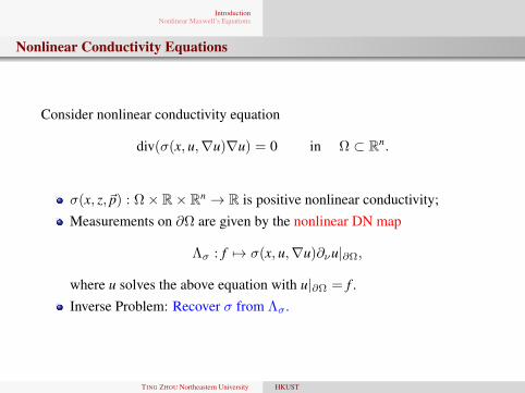
Nonlinear Conductivity Equations
Consider nonlinear conductivity equation
div(σ(x, u,∇u)∇u) = 0 in Ω ⊂ Rn.
σ(x, z,~p) : Ω× R× Rn → R is positive nonlinear conductivity;Measurements on ∂Ω are given by the nonlinear DN map
Λσ : f 7→ σ(x, u,∇u)∂νu|∂Ω,
where u solves the above equation with u|∂Ω = f .Inverse Problem: Recover σ from Λσ .
TING ZHOU Northeastern University HKUST
IntroductionNonlinear Maxwell’s Equations
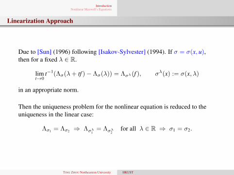
Linearization Approach
Due to [Sun] (1996) following [Isakov-Sylvester] (1994). If σ = σ(x, u),then for a fixed λ ∈ R.
limt→0
t−1(Λσ(λ+ tf )− Λσ(λ)) = Λσλ(f ), σλ(x) := σ(x, λ)
in an appropriate norm.
Then the uniqueness problem for the nonlinear equation is reduced to theuniqueness in the linear case:
Λσ1 = Λσ2 ⇒ Λσλ1 = Λσλ2 for all λ ∈ R ⇒ σ1 = σ2.
TING ZHOU Northeastern University HKUST

IntroductionNonlinear Maxwell’s Equations
Other Uniqueness Results for Nonlinear Conductivity
For certain σ = σ(x,∇u):[Hervas-Sun] (2002) for constant coefficient nonlinear terms and n = 2;[Kang-Nakamura] (2002) for
σ(x,∇u)∇u replaced by γ(x)∇u +
n∑i,j=1
cij(x)∂iu∂ju + R(x,∇u).
(∗ Higher Order Linearization.)
For p-Laplacian type equations: σ = γ(x)|∇u|p−2 with 1 < p <∞.(∗ Linearization is not helpful.)
[Salo-Guo-Kar] (2016)under monotonicity condition if n = 2;under monotonicity condition for γ close to constant if n ≥ 3.
TING ZHOU Northeastern University HKUST

IntroductionNonlinear Maxwell’s Equations
Other Nonlinear Equations
Inverse Problems were considered for other nonlinear models:Semilinear parabolic: Isakov (1993);Semilinear elliptic: Isakov-Sylvester (1994), Isakov-Nachman (1995);Elasticity: Sun-Nakamura (1994) for St. Venant-Kirchhoff model;Hyperbolic: Lorenzi-Paparoni (1990), Denisov (2007),Nakamura-Vashisth (2017).
** Comparing to the inverse problem of determining spacetime usingnonlinear wave interactions.
TING ZHOU Northeastern University HKUST

IntroductionNonlinear Maxwell’s Equations
Kerr-type NonlinearityConstruction of CGO solutionsContinue the proof for the case of Kerr-type nonlinearitySecond Harmonic Generation (SHG)
Outline
1 Introduction
2 Nonlinear Maxwell’s EquationsKerr-type NonlinearityConstruction of CGO solutionsContinue the proof for the case of Kerr-type nonlinearitySecond Harmonic Generation (SHG)
TING ZHOU Northeastern University HKUST

IntroductionNonlinear Maxwell’s Equations
Kerr-type NonlinearityConstruction of CGO solutionsContinue the proof for the case of Kerr-type nonlinearitySecond Harmonic Generation (SHG)
Nonlinear Optics
No charge and current density:
∇× E = −∂tB, ∇×H = ∂tD, div D = 0, div B = 0 in Ω× R.
E(t, x) andH(t, x) are electric and magnetic fields;D is the electric displacement and B is the magnetic induction:
D = εE + PNL(E), B = µH+MNL(H);
(∗ High energy lasers can modify the optical properties of the medium).ε, µ ∈ L∞(Ω;C) are scalar electromagnetic parameters with
Re(ε) ≥ ε0 > 0 and Re(µ) ≥ µ0 > 0;
PNL andMNL nonlinear polarization and magnetization.
TING ZHOU Northeastern University HKUST

IntroductionNonlinear Maxwell’s Equations
Kerr-type NonlinearityConstruction of CGO solutionsContinue the proof for the case of Kerr-type nonlinearitySecond Harmonic Generation (SHG)
Nonlinearity
In nonlinear optics, the polarization P(t) = χ(1)E + PNL(E)
PNL = χ(2)E2 + χ(3)E3 + · · · := P(2) + P(3) + · · ·
∗ χ(j) — j-th order nonlinear susceptibility.Second-order polarization (Noncentrosymmetric media): incident waveE = Ee−iωt + c.c. generates
P(2)(t) = 2χ(2)EE + χ(2)E2e−i2ωt + c.c.
Second harmonic generationThird-order polarization: incident waveE = E1e−iω1t + E2e−iω2t + E3e−iω3t + c.c. generates polarization withterms of frequencies
3ω1, 3ω2, 3ω3,±ω1 ± ω2 ± ω3, 2ω1 + ω2, . . . .
Sum- and difference-frequency generation.
TING ZHOU Northeastern University HKUST

IntroductionNonlinear Maxwell’s Equations
Kerr-type NonlinearityConstruction of CGO solutionsContinue the proof for the case of Kerr-type nonlinearitySecond Harmonic Generation (SHG)
Nonlinearity
Lossy media: complex valued.Equivalence to time-domain ME:
P(2) =
∫ ∞0
∫ ∞0
R(2)(τ1, τ2)E(t − τ1)E(t − τ2) dτ1 dτ2.
Using Fourier transform,
χ(2)(ω1, ω2;ω1 + ω2) =
∫ ∞0
∫ ∞0
R(2)(τ1, τ2)eiω(τ1+τ2) dτ1 dτ2.
TING ZHOU Northeastern University HKUST
IntroductionNonlinear Maxwell’s Equations
Kerr-type NonlinearityConstruction of CGO solutionsContinue the proof for the case of Kerr-type nonlinearitySecond Harmonic Generation (SHG)
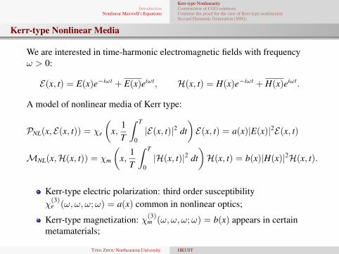
Kerr-type Nonlinear Media
We are interested in time-harmonic electromagnetic fields with frequencyω > 0:
E(x, t) = E(x)e−iωt + E(x)eiωt, H(x, t) = H(x)e−iωt + H(x)eiωt.
A model of nonlinear media of Kerr type:
PNL(x, E(x, t)) = χe
(x,
1T
∫ T
0|E(x, t)|2 dt
)E(x, t) = a(x)|E(x)|2E(x, t)
MNL(x,H(x, t)) = χm
(x,
1T
∫ T
0|H(x, t)|2 dt
)H(x, t) = b(x)|H(x)|2H(x, t).
Kerr-type electric polarization: third order susceptibilityχ
(3)e (ω, ω, ω;ω) = a(x) common in nonlinear optics;
Kerr-type magnetization: χ(3)m (ω, ω, ω;ω) = b(x) appears in certain
metamaterials;
TING ZHOU Northeastern University HKUST

IntroductionNonlinear Maxwell’s Equations
Kerr-type NonlinearityConstruction of CGO solutionsContinue the proof for the case of Kerr-type nonlinearitySecond Harmonic Generation (SHG)
Maxwell’s Equations with the Kerr-type Nonlinearity
This leads to the nonlinear time-harmonic Maxwell’s equations∇× E = iωµH + iωb|H|2H
∇× H = −iωεE − iωa|E|2E.in Ω ⊂ R3.
Electromagnetic measurements on ∂Ω are modeled by the admittance map
Λωε,µ,a,b : ν × E|∂Ω 7→ ν × H|∂Ω.
Inverse Problem: Determine ε, µ, a, b from Λωε,µ,a,b.
TING ZHOU Northeastern University HKUST

IntroductionNonlinear Maxwell’s Equations
Kerr-type NonlinearityConstruction of CGO solutionsContinue the proof for the case of Kerr-type nonlinearitySecond Harmonic Generation (SHG)
Well-posedness for the Direct Problem
Let Div be the surface divergence on ∂Ω. For 1 < p <∞, define
W1−1/p,pDiv (∂Ω) := f ∈ TW1−1/p,p(∂Ω) : Div(f ) ∈ W1−1/p,p(∂Ω),
W1,pDiv(Ω) := u ∈ W1,p(Ω) : ν × u|∂Ω ∈ W1−1/p,p
Div (∂Ω).
Theorem (Assylbekov-Z. 2017)
Let 3 < p ≤ 6. Suppose ε, µ ∈ C2(Ω) and a, b ∈ C1(Ω). If ω > 0 isnon-resonant, there is δ > 0 such that the b. v. p.
∇× E = iωµH + iωb|H|2H
∇× H = −iωεE − iωa|E|2E
ν × E|∂Ω = f ∈ W1−1/p,pDiv (∂Ω) with ‖f‖W1−1/p,p
Div (∂Ω)< δ
has a unique solution (E,H) ∈ W1,pDiv(Ω)×W1,p
Div(Ω).
∗ The proof is based on the Sobolev embedding and the contraction mappingargument.
TING ZHOU Northeastern University HKUST

IntroductionNonlinear Maxwell’s Equations
Kerr-type NonlinearityConstruction of CGO solutionsContinue the proof for the case of Kerr-type nonlinearitySecond Harmonic Generation (SHG)
Main Result for the Inverse Problem
Theorem (Assylbekov-Z. 2017)
Let 4 ≤ p < 6. Suppose εj, µj ∈ C2(Ω) and aj, bj ∈ C1(Ω), j = 1, 2. Fix anon-resonant ω > 0 and small enough δ > 0. If
Λωε1,µ1,a1,b1(f ) = Λωε2,µ2,a2,b2
(f )
for all f ∈ W1−1/p,pDiv (∂Ω) with ‖f‖W1−1/p,p
Div (∂Ω)< δ, then
ε1 = ε2, µ1 = µ2, a1 = a2, b1 = b2.
TING ZHOU Northeastern University HKUST
IntroductionNonlinear Maxwell’s Equations
Kerr-type NonlinearityConstruction of CGO solutionsContinue the proof for the case of Kerr-type nonlinearitySecond Harmonic Generation (SHG)
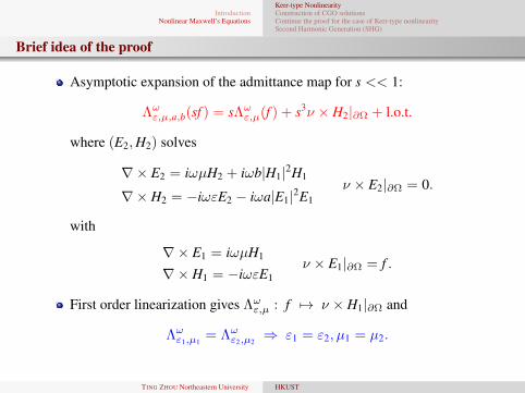
Brief idea of the proof
Asymptotic expansion of the admittance map for s << 1:
Λωε,µ,a,b(sf ) = sΛωε,µ(f ) + s3ν × H2|∂Ω + l.o.t.
where (E2,H2) solves
∇× E2 = iωµH2 + iωb|H1|2H1
∇× H2 = −iωεE2 − iωa|E1|2E1ν × E2|∂Ω = 0.
with
∇× E1 = iωµH1
∇× H1 = −iωεE1ν × E1|∂Ω = f .
First order linearization gives Λωε,µ : f 7→ ν × H1|∂Ω and
Λωε1,µ1= Λωε2,µ2
⇒ ε1 = ε2, µ1 = µ2.
TING ZHOU Northeastern University HKUST

IntroductionNonlinear Maxwell’s Equations
Kerr-type NonlinearityConstruction of CGO solutionsContinue the proof for the case of Kerr-type nonlinearitySecond Harmonic Generation (SHG)
Brief idea of the proof
Third order linearization gives the map
∂3s Λωε,µ,a,b : f = ν × E1|∂Ω 7→ ν × H2|∂Ω.
We derive an integral identity from ∂3s Λωε,µ,a1,b1
= ∂3s Λωε,µ,a2,b2∫
Ω
(a1 − a2)|E1|2E1 · E dx +
∫Ω
(b1 − b2)|H1|2H1 · H dx = 0
for all (E1,H1) and (E, H) solving
∇× E1 = iωµH1,
∇× H1 = −iωεE1,and
∇× E = iωµH,
∇× H = −iωεE,
where ε = ε1 = ε2 and µ = µ1 = µ2.
TING ZHOU Northeastern University HKUST

IntroductionNonlinear Maxwell’s Equations
Kerr-type NonlinearityConstruction of CGO solutionsContinue the proof for the case of Kerr-type nonlinearitySecond Harmonic Generation (SHG)
Construction of CGO solutions [Ola-Somersalo]
∇× E − iωµH = 0∇ · (µH) = 0
∇× H + iωεE = 0∇ · (εE) = 0
=⇒
Φ =i
ωµε∇ · (εE)
∇× E − iωµH − 1ε∇εΨ = 0
Ψ =i
ωµε∇ · (µH)
∇× H + iωεE +1µ∇µΦ = 0
Set X = (µ1/2Φ, µ1/2Ht, ε1/2Ψ, ε1/2Et)t ↓ Liouville type of↓ rescaling
(P− k + W)X = 0 an elliptic first order system
TING ZHOU Northeastern University HKUST
IntroductionNonlinear Maxwell’s Equations
Kerr-type NonlinearityConstruction of CGO solutionsContinue the proof for the case of Kerr-type nonlinearitySecond Harmonic Generation (SHG)
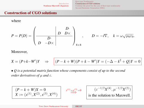
Construction of CGO solutions
where
P = P(D) =
D·
D D×D·
D −D×
8×8
, D = −i∇, k = ω√µ0ε0.
Moreover,
X = (P+k−W t)Y ⇒ (P− k + W)(P + k −W t)Y = (−∆− k2 + Q)Y = 0
• Q is a potential matrix function whose components consist of up to the secondorder derivatives of µ and ε.
(P− k + W)X = 0X := (x(1),X(2), x(3),X(4))
x(1)=x(3)=0=⇒
(ε−1/2X(4), µ−1/2X(2))
is the solution to Maxwell.
TING ZHOU Northeastern University HKUST
IntroductionNonlinear Maxwell’s Equations
Kerr-type NonlinearityConstruction of CGO solutionsContinue the proof for the case of Kerr-type nonlinearitySecond Harmonic Generation (SHG)
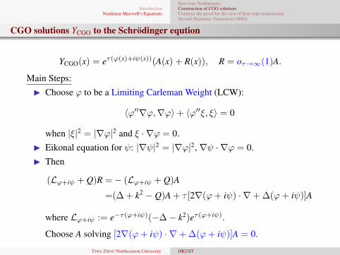
CGO solutions YCGO to the Schrödinger eqution
YCGO(x) = eτ(ϕ(x)+iψ(x))(A(x) + R(x)), R = oτ→∞(1)A.
Main Steps:I Choose ϕ to be a Limiting Carleman Weight (LCW):
〈ϕ′′∇ϕ,∇ϕ〉+ 〈ϕ′′ξ, ξ〉 = 0
when |ξ|2 = |∇ϕ|2 and ξ · ∇ϕ = 0.I Eikonal equation for ψ: |∇ψ|2 = |∇ϕ|2,∇ψ · ∇ϕ = 0.I Then
(Lϕ+iψ + Q)R =− (Lϕ+iψ + Q)A
=(∆ + k2 − Q)A + τ [2∇(ϕ+ iψ) · ∇+ ∆(ϕ+ iψ)]A
where Lϕ+iψ := e−τ(ϕ+iψ)(−∆− k2)eτ(ϕ+iψ).
Choose A solving [2∇(ϕ+ iψ) · ∇+ ∆(ϕ+ iψ)]A = 0.
TING ZHOU Northeastern University HKUST

IntroductionNonlinear Maxwell’s Equations
Kerr-type NonlinearityConstruction of CGO solutionsContinue the proof for the case of Kerr-type nonlinearitySecond Harmonic Generation (SHG)
CGO solutions to the Schrödinger equation
I Last step: Solving
(Lϕ+iψ + Q)R = (∆ + k2 − Q)A
[Sylvester-Uhlmann,1987]: τ(ϕ+ iψ) = ζ · x where ζ ∈ Cn,ζ · ζ = −k2, |ζ| ∼ τ . A is constant. Solve
(−∆− 2ζ · ∇+ Q)R = −QA
globally using estimate ‖(−∆− 2ζ · ∇)−1‖ ∼ O(τ−1).[Kenig-Sjöstrand-Uhlmann,2007]: Nonlinear LCW ϕ(x) = − ln |x|[Kenig-Salo-Uhlmann,2012]: LCW ϕ(x) = −x1, ψ(x) is linear in thetransverse polar coordinate r = (x2
2 + x23)1/2.
TING ZHOU Northeastern University HKUST

IntroductionNonlinear Maxwell’s Equations
Kerr-type NonlinearityConstruction of CGO solutionsContinue the proof for the case of Kerr-type nonlinearitySecond Harmonic Generation (SHG)
ϕ(x) = −x1 and ϕ(x) = − ln |x|
Set z = x1 + ir, where x = (x1, r, θ) denotes the cylindrical coordinate.LCW ϕ(x) = −x1 = <(z) → ϕ+ iψ = l(z) = −z.
l′(z)(
2∂z −1
z− z
)A = 0, we take A =
eiλz√
2irg(θ).
LCW ϕ(x) = − ln |x| = −<(ln z) → ϕ+ iψ = l(z) = − ln z.
l′(z)(
2∂z +1
z− z
)A = 0, we take A =
eiλz√
2irg(θ).
I In both cases, a semi-classical Carleman estimate on a bounded domaincan be derived as an a-priori estimate for the adjoint operator L∗ϕ+iψ (see e.g.[Kenig-Sjöstrand -Uhlmann,2007]), in order to prove both the existence andsmallness of R (relative to A) for τ large.I g(θ) is an arbitrary 8-vector function.
TING ZHOU Northeastern University HKUST

IntroductionNonlinear Maxwell’s Equations
Kerr-type NonlinearityConstruction of CGO solutionsContinue the proof for the case of Kerr-type nonlinearitySecond Harmonic Generation (SHG)
CGO solutions for Maxwell’s equations
We have
XCGO = (P + k −W t)[eτ(ϕ+iψ)(A + R)]
= eτ(ϕ+iψ) τP(D(ϕ+ iψ))A + (P + k −W t)A
+τP(D(ϕ+ iψ))R + (P + k −W t)R:= eτ(ϕ+iψ)(B + S)
Recall that we need x(1) = x(3) = 0.I Choose g(θ) such that b(1) = b(3) = 0.I To show s(1) = s(3) = 0, use
(P + k −W t)(P− k + W)X = (−∆− k2 + Q)X = 0
where only Q11 and Q33 are nonzero in their corresponding rows.
=⇒ (Lϕ+iψ + Qkk)s(k) = 0, k = 1, 3.
?=⇒ s(k) = 0.
TING ZHOU Northeastern University HKUST

IntroductionNonlinear Maxwell’s Equations
Kerr-type NonlinearityConstruction of CGO solutionsContinue the proof for the case of Kerr-type nonlinearitySecond Harmonic Generation (SHG)
Uniqueness for Lϕ+iψ
For linear phase ζ · x, uniqueness is obtained globally assumingdecaying at infinity. (see [Sylvester-Uhlmann, 1987]);For ϕ(x) + iψ(x) = −(x1 + ir), uniqueness is obtained on a cylinderT = R× B(0,R) for B(0,R) ⊂ R2 assuming zero Dirichlet conditionand decaying at infinities of x1 direction. (see [Kenig-Salo-Uhlmann,2012]);For ϕ(x) + iψ(x) = − ln z, following [Nachman-Street, 2002], wedecompose L2(Ω) as
L∗ϕ+iψv ∈ S(Rn) : supp(v) ⊂ Ω. ⊕W
Then we can show the uniqueness by choosing S as above.
TING ZHOU Northeastern University HKUST

IntroductionNonlinear Maxwell’s Equations
Kerr-type NonlinearityConstruction of CGO solutionsContinue the proof for the case of Kerr-type nonlinearitySecond Harmonic Generation (SHG)
Try CGO solutions with linear phases
Recall the integral identity∫Ω
(a1 − a2)|E1|2E1 · E dx +
∫Ω
(b1 − b2)|H1|2H1 · H dx = 0
Complex Geometrical Optics solutions with linear phases
E1(x) = ε−1/2eζ1·x(
s0ζ1 · α|ζ1|
ζ1 + o|ζ1|→∞(|ζ1|))
H1(x) = µ−1/2eζ1·x(
t0ζ1 · β|ζ1|
ζ1 + o|ζ1|→∞(|ζ1|)) as |ζ1| → ∞.
where for ξ = (ξ1, 0, 0), ξ1 ∈ R,
ζ1 =
(iξ1,−
√ξ2
1/4 + τ 2, i√τ 2 − k2
)⇒ ζ1 · ζ1 = k2, |ζ1| ∼ τ.
s0 = 1, t0 = 0: the leading term of |E1|2E1 · E does not provide enoughF.T. of (a1 − a2);
TING ZHOU Northeastern University HKUST

IntroductionNonlinear Maxwell’s Equations
Kerr-type NonlinearityConstruction of CGO solutionsContinue the proof for the case of Kerr-type nonlinearitySecond Harmonic Generation (SHG)
Polarization
In the integral identity, we plug in
(E1,H1) = (E(1) + E(2) + E(3),H(1) + H(2) + H(3))
where (E(j),H(j)) are solutions to the linear equations. Then∫Ω
(a1 − a2)[<(E(3) · E(2))(E(1) · E) + <(E(3) · E(1))(E(2) · E)
+ <(E(1) · E(2))(E(3) · E)]
dx
+
∫Ω
(b1 − b2)[<(H(3) · H(2))(H(1) · H) + <(H(3) · H(1))(H(2) · H)
+ <(H(1) · H(2))(H(3) · H)]
dx = 0
TING ZHOU Northeastern University HKUST
IntroductionNonlinear Maxwell’s Equations
Kerr-type NonlinearityConstruction of CGO solutionsContinue the proof for the case of Kerr-type nonlinearitySecond Harmonic Generation (SHG)
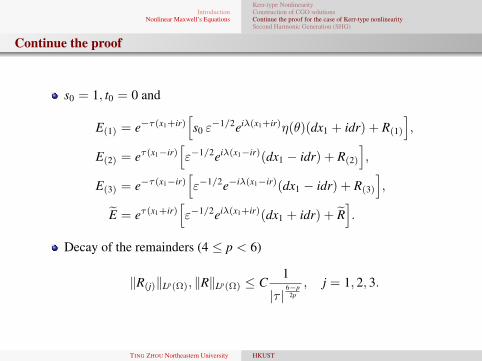
Continue the proof
s0 = 1, t0 = 0 and
E(1) = e−τ(x1+ir)[s0 ε−1/2eiλ(x1+ir)η(θ)(dx1 + idr) + R(1)
],
E(2) = eτ(x1−ir)[ε−1/2eiλ(x1−ir)(dx1 − idr) + R(2)
],
E(3) = e−τ(x1−ir)[ε−1/2e−iλ(x1−ir)(dx1 − idr) + R(3)
],
E = eτ(x1+ir)[ε−1/2eiλ(x1+ir)(dx1 + idr) + R
].
Decay of the remainders (4 ≤ p < 6)
‖R(j)‖Lp(Ω), ‖R‖Lp(Ω) ≤ C1
|τ |6−p
2p
, j = 1, 2, 3.
TING ZHOU Northeastern University HKUST

IntroductionNonlinear Maxwell’s Equations
Kerr-type NonlinearityConstruction of CGO solutionsContinue the proof for the case of Kerr-type nonlinearitySecond Harmonic Generation (SHG)
Continue the proof
Plugging in the integral identity, as τ →∞,∫ ((a1 − a2)χΩ
|ε|2
)e−i2λ(x1−ir)η(θ) dx1 dr dθ = 0.
Set f := (a1−a2)χΩ
|ε|2 and let η(θ) ∈ C∞(S1) vary.∫ ∞0
e−2λr f (2λ, r, θ) dr = 0, θ ∈ S1.
Attenuated geodesic ray transform on R2
⇒ f = 0 ⇒ a1 = a2.Generalization to the inverse problems on admissible transversallyanisotropic manifolds.
TING ZHOU Northeastern University HKUST

IntroductionNonlinear Maxwell’s Equations
Kerr-type NonlinearityConstruction of CGO solutionsContinue the proof for the case of Kerr-type nonlinearitySecond Harmonic Generation (SHG)
Extended result
In [Cârstea, 2018], the framework is extended to prove the uniqueness indetermining
PNL =
∞∑k=1
ak(x)|E|2kE , MNL =
∞∑k=1
bk(x)|H|2kH.
∫Ω
(ak − a′k)[(e0 · e1)(e2 · e3)k + k(e0 · e2)(e1 · e3)(e2 · e3)k−1]
− (bk − b′k)[(h0 · h1)(h2 · h3)k + k(h0 · h2)(h1 · h3)(h2 · h3)k−1] dx = 0.
TING ZHOU Northeastern University HKUST

IntroductionNonlinear Maxwell’s Equations
Kerr-type NonlinearityConstruction of CGO solutionsContinue the proof for the case of Kerr-type nonlinearitySecond Harmonic Generation (SHG)
Nonlinearity in Second Harmonic Generation
Incident beam: E(t, x) = E0(x)e−itω + c.c.Writing the solution to include terms at frequency ω and 2ω:
E(t, x) = 2Re
Eω(x)e−iωt+ 2Re
E2ω(x)e−i2ωtH(t, x) = 2Re
Hω(x)e−iωt+ 2Re
H2ω(x)e−i2ωt ,
Then we obtain the system∇× Eω − iωµHω = 0,
∇× Hω + iωεEω + iωχ(2)Eω · E2ω = 0,
∇× E2ω − i2ωµH2ω = 0,
∇× H2ω + i2ωεE2ω + i2ωχ(2)Eω · Eω = 0.
(1)
∗ One can also introduce the similar nonlinear second harmonic generationeffect for magnetic fields;
∗ Here we can also assume that µ, ε depend on the frequency.
TING ZHOU Northeastern University HKUST

IntroductionNonlinear Maxwell’s Equations
Kerr-type NonlinearityConstruction of CGO solutionsContinue the proof for the case of Kerr-type nonlinearitySecond Harmonic Generation (SHG)
Applications
SHG can be so efficient that nearly all of the power in the incidentbeam at frequency ω is converted to radiation at the frequency 2ω;Second harmonic generation microscopy for noncentrosymmetricmedia.
TING ZHOU Northeastern University HKUST

IntroductionNonlinear Maxwell’s Equations
Kerr-type NonlinearityConstruction of CGO solutionsContinue the proof for the case of Kerr-type nonlinearitySecond Harmonic Generation (SHG)
Well-posedness for the Direct Problem
Theorem
Let 3 < p ≤ 6. Suppose that ε, µ ∈ C2(Ω;C) are complex-valued functionswith positive real parts and χ(2) ∈ C1(Ω;R3). For every ω ∈ C, outside adiscrete set Σ ⊂ C of resonant frequencies, there is δ > 0 such that for a
pair (fω, f 2ω) ∈(
TW1−1/p,pDiv (∂M)
)2with
∑k=1,2
‖f kω‖TW1−1/p,p
Div (∂Ω)< δ, the
Maxwell’s equations (1) has a unique solution
(Eω,Hω,E2ω,H2ω) ∈(
W1,pDiv(Ω)
)4satisfying ν × Ekω|∂Ω = f kω for
k = 1, 2 and∑k=1,2
‖Ekω‖W1,p
Div(Ω) + ‖Hkω‖W1,p
Div(Ω) ≤ C∑
k=1,2
‖f kω‖TW1−1/p,p
Div (∂Ω),
for some constant C > 0 independent of (fω, f 2ω).
TING ZHOU Northeastern University HKUST

IntroductionNonlinear Maxwell’s Equations
Kerr-type NonlinearityConstruction of CGO solutionsContinue the proof for the case of Kerr-type nonlinearitySecond Harmonic Generation (SHG)
Inverse Problem
Admittance Map:
Λω,2ωε,µ,χ(2)(fω, f 2ω) =
(ν × Hω|∂Ω, ν × H2ω|∂Ω
),
Theorem
Let 4 ≤ p < 6. Suppose that εj ∈ C3(Ω;C), µj ∈ C2(Ω;C) with positivereal parts and χ(2)
j ∈ C1(Ω;R3), j = 1, 2. Fix ω > 0 outside a discrete set ofresonant frequencies Σ ⊂ C and fix sufficiently small δ > 0. If
Λω,2ωε1,µ1,χ
(2)1
(fω, f 2ω) = Λω,2ωε2,µ2,χ
(2)2
(fω, f 2ω)
for all (fω, f 2ω) ∈(
TW1−1/p,pDiv (∂Ω)
)2with
∑k=1,2
‖f kω‖TW1−1/p,p
Div (∂Ω)< δ,
then ε1 = ε2, µ1 = µ2, χ(2)1 = χ
(2)2 in Ω.
TING ZHOU Northeastern University HKUST

IntroductionNonlinear Maxwell’s Equations
Kerr-type NonlinearityConstruction of CGO solutionsContinue the proof for the case of Kerr-type nonlinearitySecond Harmonic Generation (SHG)
Brief idea of the proof
Asymptotic expansion of the admittance map for s << 1:
Λω,2ωε,µ,χ(2)(sfω, sf 2ω) = sΛω,2ωε,µ (fω, f 2ω)+s2(ν×Hω
2 |∂Ω, ν×H2ω2 |∂Ω)+l.o.t.
where (Eω2 ,Hω2 ,E
2ω2 ,H2ω
2 ) solves∇× Ekω
2 − ikωµHkω2 = 0, k = 1, 2,
∇× Hω2 + iωεEω2 + iωχ(2)Eω1 · E
2ω1 = 0,
∇× H2ω2 + i2ωεE2ω
2 + iωχ(2)Eω1 · Eω1 = 0,
ν × Ekω2 |∂Ω = 0, k = 1, 2.
with
∇× Ekω1 − ikωµHkω
1 = 0, ∇× Hkω1 + ikωεEkω
1 = 0,
ν × Ekω1 |∂Ω = f kω, k = 1, 2.
Linearization gives Λω,2ωε1,µ1= Λω,2ωε2,µ2
⇒ ε1 = ε2 and µ1 = µ2;
TING ZHOU Northeastern University HKUST

IntroductionNonlinear Maxwell’s Equations
Kerr-type NonlinearityConstruction of CGO solutionsContinue the proof for the case of Kerr-type nonlinearitySecond Harmonic Generation (SHG)
Brief idea of the proof
Using the second order term, the map
(fω, f 2ω) 7→ (ν × Hω2 |∂Ω, ν × H2ω
2 |∂Ω)
we derive a nonlinear integral identity∫χΩ
(χ
(2)1 − χ
(2)2
)·[ (
Eω1 · E2ω1
)Eω + 2
(Eω1 · Eω1
)E2ω]
dx = 0
for all (Eω1 ,Hω1 ,E
2ω1 ,H2ω
1 ) and (Eω, Hω, E2ω, H2ω) solving the linearequations with µ = µ1 = µ2 and ε = ε1 = ε2.∗ No polarization is needed since linear equations for Eω and E2ω are
decoupled.
Plug in CGO solutions from [Ola-Päivärinta-Sommersalo],
TING ZHOU Northeastern University HKUST

IntroductionNonlinear Maxwell’s Equations
Kerr-type NonlinearityConstruction of CGO solutionsContinue the proof for the case of Kerr-type nonlinearitySecond Harmonic Generation (SHG)
Continue the proof
For ξ = ξ1e1, choose
ζω1 =
i ξ12
−√
ξ21
4 + τ 2
i√τ 2 − k2
, Eω1 = eζω1 ·x
11√
ξ21
4 +τ 2−i ξ12
i√τ 2−k2
+ Rω1
ζ2ω1 =
−iξ1
2√
ξ21
4 + τ 2
2i√τ 2 − k2
, E2ω1 = eζ
2ω1 ·x
11
iξ1−2
√ξ2
14 +τ 2
2i√τ 2−k2
+ R2ω1
ζω =
i ξ12
−√
ξ21
4 + τ 2
−i√τ 2 − k2
, Eω = eζω·x[Aω + Rω
](Eω1 · E
2ω1
)Eω = e−iξ·x(Aω + l.o.t.)
Choose ζ2ω such that 2(Eω1 · Eω1 )E2ω decays exponentially in τ .TING ZHOU Northeastern University HKUST
IntroductionNonlinear Maxwell’s Equations
Kerr-type NonlinearityConstruction of CGO solutionsContinue the proof for the case of Kerr-type nonlinearitySecond Harmonic Generation (SHG)
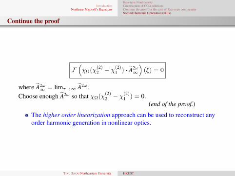
Continue the proof
F(χΩ(χ
(2)2 − χ
(2)1 ) · A2ω
∞
)(ξ) = 0
where A2ω∞ = limτ→∞ A2ω .
Choose enough A2ω so that χΩ(χ(2)2 − χ
(2)1 ) = 0.
(end of the proof.)
The higher order linearization approach can be used to reconstruct anyorder harmonic generation in nonlinear optics.
TING ZHOU Northeastern University HKUST

IntroductionNonlinear Maxwell’s Equations
Kerr-type NonlinearityConstruction of CGO solutionsContinue the proof for the case of Kerr-type nonlinearitySecond Harmonic Generation (SHG)
Some recent scalar case results (semi-linear equations)
[Lassas-Liimantainen-Lin-Salo], [Feizmohammadi-Oksanen]
∆u + a(x, u) = 0, x ∈ Ω
where a(x, z) satisfiesa(x, 0) = 0 and 0 is not a Dirichlet eigenvalue to ∆ + ∂za(x, 0) in Ωa(x, 0) = ∂za(x, 0) = 0 (Using non-CGO solutions,[Krupchyk-Uhlmann])a(x, z) is analytic in z: a(x, z) =
∑∞k=1 ak(x) zk
k! .
(∗ Simultaneously reconstruct inclusions/obstacles and the backgroundcoefficients; Partial data problems)
TING ZHOU Northeastern University HKUST

IntroductionNonlinear Maxwell’s Equations
Kerr-type NonlinearityConstruction of CGO solutionsContinue the proof for the case of Kerr-type nonlinearitySecond Harmonic Generation (SHG)
Future work
Implement other solutions.Partial data problems.
TING ZHOU Northeastern University HKUST

IntroductionNonlinear Maxwell’s Equations
Kerr-type NonlinearityConstruction of CGO solutionsContinue the proof for the case of Kerr-type nonlinearitySecond Harmonic Generation (SHG)
Thanks for your attention!
TING ZHOU Northeastern University HKUST