diploma thesis: development and validation of a...
TRANSCRIPT
Diploma Thesis:
Development and validation of a plant model for
Battery Monitoring Systems (BMS) for high voltage
batteries
By
Cédric, Ange-Etienne ACQUAVIVA
Electrical engineering
Option: energy
March 2012 – August 2012
Supervisor INSA Strasbourg:
Jean-Michel Hubé
Supervisors Deutsche ACCUmotive GmbH & Co. KG: Bachelor of Engineering, Timo Steinke
Diploma Engineering, Roger Steller
September, 2012
II
Summarize
Deutsche ACCUmotive develops and produces high voltage batteries for electric cars. The
batteries are equipped with their battery management system (BMS). The software of this
electronic device is tested by the software team with the hardware-In-the-Loop (HIL)
process.
Among this team, the subject of the thesis was the further development and validation of
the Simulink plant model. That is needed to test the BMS, which is intern incorporated into
the battery of the “smart fortwo electric drive”. The objective was to implement the battery
cooling, the battery charge process, the control of the discharge current and the network
management. The validation of the model was performed on a Hardware-In-the-Loop test
bench with the real BMS.
To reach the objective, the electronic devices responsible for these functionalities were first
studied and then the existing model was tested. From these 2 tasks, the specific functions to
be implemented were found out and programmed in Simulink. The model was checked in
the Simulink environment and finally on the HIL test bench with the real BMS. To perform
these tests, relevant scenarios were imagined.

III
Objectives
Subject description
Development and validation of a plant model for the BMS designed for the high voltage
battery of the “smart fortwo electric drive”.
This model is an essential element of the hardware-in-the-loop test bench allowing the test
of the BMS software.
Objectives
- To implement the cooling of the battery
- To implement the network management with the protocol OSEK and AUTOSAR
- To implement the energy management function block (charge process, battery
security)
- To implement the on board charger block
- To test the model in its Simulink environment
- To imagine test scenarios for the tests with the BMS
- To validate the model with the real BMS
Supervisors of the thesis
Bachelor of Engineering, Timo Steinke
Diploma of Engineering, Roger Steller
IV
Acknowledgements
Je remercie mes parents Linda et Charles et ma petite sœur Laetitia qui m’ont accompagné
dans mes choix. Je tiens aussi à remercier aussi mon grand-père Stéphan pour m’avoir
toujours conseillé et soutenu.
Ich danke meinen Betreuern Timo und Roger dafür, dass sie mir diese Abschlussarbeit
anvertraut haben. Ich habe durch diese Abschlussarbeit viel gelernt und entdeckt.
Ich vergesse auch Torben nicht, der mir viel bei der Kühlung geholfen hat.
Mit Johannes hat es auch Spaß gemacht, HIL-Tests durchzuführen.
Ich danke Brahim für seine Hilfe bei der Implementierung des network managements.
Ich danke auch meinen Kollegen Bhagyesh, Max, Andy, Christian, Simon, Jakob, Rajeed für
die tolle Stimmung und die gute Momente.

V
Table of content
Summarize .................................................................................................................................. II
Objectives .................................................................................................................................. III
Acknowledgements ................................................................................................................... IV
List of figures ............................................................................................................................ VII
List of abbreviations ................................................................................................................... 9
BMS : Battery Management System ................................................................................... 9
Introduction .............................................................................................................................. 10
1 Global presentation of the project ................................................................................... 12
1.1 Presentation of the “smart fortwo electric drive” [3] ............................................... 12
1.2 Lithium-ion battery .................................................................................................... 14
1.2.1 Main advantages and limitations ....................................................................... 14
1.2.2 State of Charge ................................................................................................... 15
1.2.3 Charge of the battery ......................................................................................... 15
1.3 Battery Management System BMS ........................................................................... 16
1.3.1 BMS tasks ........................................................................................................... 16
1.3.2 Architecture of the BMS ..................................................................................... 16
2 Presentation of the way of testing ................................................................................... 18
2.1 Goal of the test process ............................................................................................. 18
2.1.1 Principle .............................................................................................................. 18
2.1.2 Advantages ......................................................................................................... 18
2.2 Test components ....................................................................................................... 18
2.3 Control of the inputs/outputs of the model.............................................................. 19
2.3.1 Database with Vector CANdb++ [9] ................................................................... 19
2.3.2 Vector CANoe and the box Vector VN8970 [10] ................................................ 19
2.3.3 Graphical user interface with the software MBtech PROVEtechTA .................. 20
2.4 Presentation of the model ......................................................................................... 21
3 Implementation of the different blocks ........................................................................... 24
3.1 Common Powertrain Controller (CPC) ...................................................................... 24
3.1.1 Cooling elements ................................................................................................ 24

VI
3.1.2 Simulation of the battery cooling....................................................................... 26
3.1.3 CPC Simulink block implementation .................................................................. 27
3.1.4 Implementation .................................................................................................. 28
3.1.5 Choice of power ................................................................................................. 32
3.1.6 Test of the power calculation ............................................................................. 34
3.2 Cell-model .................................................................................................................. 37
3.3 Network management (NM) ..................................................................................... 37
3.3.1 Protocol OSEK [12] ............................................................................................. 38
3.3.2 AUTOSAR ............................................................................................................ 41
3.4 Energy management (EMM) and on board charger (OBL) ........................................ 42
3.4.1 Input signals ....................................................................................................... 42
3.4.2 Output signals .................................................................................................... 43
3.4.3 Power prediction from the BMS ........................................................................ 43
3.4.4 Structure of the module ..................................................................................... 44
3.5 On board charger ....................................................................................................... 47
4 Tests ................................................................................................................................. 48
4.1 Cooling module .......................................................................................................... 48
4.1.1 Scenarios ............................................................................................................ 48
4.1.3 Offline test .......................................................................................................... 50
4.1.4 Online Test ......................................................................................................... 50
4.2 Energy management and on board charger module ................................................ 51
4.2.1 Scenarios ............................................................................................................ 51
4.2.2 Offline tests ........................................................................................................ 51
4.2.3 Online tests ........................................................................................................ 53
4.3 Network management ............................................................................................... 54
4.3.1 OSEK ................................................................................................................... 54
4.3.2 AUTOSAR ............................................................................................................ 56
4.3.3 Offline tests ........................................................................................................ 56
4.4 Online test ................................................................................................................. 57
Conclusion ................................................................................................................................ 58
References ................................................................................................................................ 59
VII
List of figures
Figure 1-1: Smart in a charge station ....................................................................................... 12
Figure 1-2: Power architecture of the ev-smart....................................................................... 13
Figure 1-3: vehicle-Can of the electric SMART [4] ................................................................... 13
Figure 1-4: energy density comparison [5] .............................................................................. 14
Figure 1-5: Operation limits of lithium-ion battery [6] ............................................................ 14
Figure 1-6: determination of the SOC with the Opened Circuit Voltage (OCV)[7] .................. 15
Figure 1-7: charging process .................................................................................................... 15
Figure 1-8: BMS architecture [8] .............................................................................................. 17
Figure 2-1: Model and the BMS in a closed loop ..................................................................... 18
Figure 2-2: test bench .............................................................................................................. 19
Figure 2-3: box Vector VN8970 ................................................................................................ 20
Figure 2-4: CANoe simulation and real device ......................................................................... 20
Figure 2-5: User interface MBtechPROVEtechTA .................................................................... 21
Figure 2-6: structure of the Simulink model ............................................................................ 21
Figure 2-7: mapping of signals ................................................................................................. 22
Figure 2-8: overview of the plant model .................................................................................. 23
Figure 3-1: cooling circuits [11] ................................................................................................ 24
Figure 3-2: Normal way of cooling ........................................................................................... 25
Figure 3-3: AC-cooling .............................................................................................................. 25
Figure 3-4: choice of cooling in function of the battery temperature ..................................... 26
Figure 3-5: simplified process of cooling .................................................................................. 27
Figure 3-7: CPC block ................................................................................................................ 29
Figure 3-8: pumps and air flow rates ....................................................................................... 30
Figure 3-9: Temperature into a percentage conversion .......................................................... 30
Figure 3-10: determination of air flow rate table .................................................................... 31
Figure 3-11: temperature of the coolant exchange ................................................................. 32
Figure 3-12: Cooling Power calculation (normal way of cooling) ............................................ 32
Figure 3-13: Choice of the power ............................................................................................. 33
Figure 3-14: inputs and outputs for the charging and drive mode .......................................... 33
Figure 3-15: cooling power in function of time ....................................................................... 34
Figure 3-16: cooling power in W in function of time ............................................................... 35
Figure 3-17: cooling Power in W function of the battery temperature in °C .......................... 36
Figure 3-18: cell model ............................................................................................................. 37
Figure 3-19: OSEK communication process ............................................................................. 38
Figure 3-20: Embedded simulation controlled by the Simulink model ................................... 39
Figure 3-21: ev-can (CANoe screenshot) .................................................................................. 39
Figure 3-22: NM message from OBL called NM_OBL and its signals ....................................... 40
Figure 3-23: command message (VectorCANdb++) ................................................................. 40
VIII
Figure 3-24: Simulinkstate machine for one node ................................................................... 41
Figure 3-25: ev-can AUTOSAR .................................................................................................. 42
Figure 3-26: Energy management module ............................................................................... 42
Figure 3-27: structure of the energy management module .................................................... 44
Figure 3-28: states machine ..................................................................................................... 45
Figure 3-29: charge algorithm .................................................................................................. 46
Figure 3-30: Charge current request ........................................................................................ 47
Figure 4-1: Simulink model for offline tests ............................................................................. 48
Figure 4-2: cooling with a -100A discharge current ................................................................. 50
Figure 4-3: Battery charge ........................................................................................................ 52
Figure4-4: complete discharge and partial charges/discharges .............................................. 53
Figure 4-5: charge current limits test ....................................................................................... 54
Figure 4-6: ring between OBL and CPC .................................................................................... 55
Figure 4-7: test installation ...................................................................................................... 55
Figure 4-8: nodes in the suspended mode ............................................................................... 56
Figure 4-9:getState returns and CAN signals ........................................................................... 57
Figure 4-10: installation of the AUTOSAR network management simulation ......................... 57

9
List of abbreviations
BMS : Battery Management System
CPC : Common Power Train Controller
EMM : Energy Management
NM : Network Management
OCV : Open Circuit Voltage
ECU : Electronic Control Unit
10
Introduction
Due to the current global warming phenomenon in environment, the reduction of CO2
emission by vehicles has gained special interest. Since the electric car does not emit CO2 by
driving, it could be a feasible solution for the future. This leads to the booming interest in
the research for electric cars. Big car companies are now developing more and more electric
models, for instance Daimler has the “Smart fortwo” and Renault the “Twingo”.
The lithium-ion battery is a key technology for these cars. In order to improve its
competences in this technology, Daimler AG along with Evonik industries AG created a joint
venture called Deutsche ACCUmotive. Evonik possess 10% of Deutsche ACCUmotive and
Daimler 90% [1].
Evonik is a chemical industry company. Since Evonik along with Daimler has a sub-company
called Li-Tec which produces cells for car batteries, the joint venture makes sense [2].
Deutsche ACCUmotive delivers complete batteries for the Daimler electric and hybrid cars.
The delivered batteries come equipped with Li-Tec cells and with Deutsche ACCUmotive
battery management system (BMS). The task of the BMS is to improve the performances and
the life time of the battery.
About 140 workers in 2 locations work for Deutsche ACCUmotive. The batteries are
produced in Kammenz. The development center in Nabern is responsible for the batteries
and the BMS design. It is also in Nabern, that the software of the BMS is implemented and
tested.
The thesis took place in the software team by Deutsche ACCUmotive in Nabern. The purpose
was to continue the development and validate the Simulink model allowing the testers to
check the software of the BMS designed for the high voltage batteries of the electric car
“smart fortwo”.
The model has to simulate the battery and the electronic devices which communicate with
the BMS. This model is essential, because it interacts in real time with the BMS. In this way,
the model sends signals to the BMS, and the response of the BMS can be analyzed.
The objective was to implement in Simulink the cooling circuit of the battery, the battery
charge process, the control of the discharge current and the network management. To
program these functionalities, the concerned electronic devices were first studied and the
existing model was tested. From these 2 tasks, the specific functions to be implemented
were found out and programmed. The model was checked in the Simulink environment and
finally on the HIL test bench with the actual BMS.

11
The first part of the thesis presents the global project, in order to have an overview of the
components of the “smart fortwo” and to understand why the BMS is necessary. The second
part explains the HIL process used in the BMS tests, and the structure of the model. The
third part concerns the ECUs which were implemented during the thesis. The fourth will
present the tests performed.

12
1 Global presentation of the project
The purpose of this chapter is to understand why the Battery Management System (BMS) is
essential for lithium-ion batteries. Since the BMS of the thesis is developed for the “smart
fortwo electric drive”, this car is first presented.
1.1 Presentation of the “smart fortwo electric drive” [3]
The “smart fortwo” must be launched in September 2012. This is an all-electric car produced
by Daimler AG. This model is the third generation; the first one was tested in 2007.
Its power source is a Lithium-ion battery developed by the company Deutsche ACCUmotive.
It is composed of 3 modules of 31 cells connected in serial. The nominal capacity is 52 Ah
and the maximum voltage is 391V. Its energy is about 18kWh, the consumption is about 15.1
kWh/100km. A maximum power of about 77 kW can be provided.
The battery can be charged from every 230V alternative power source at home or in every
charge station (figure 1-1).
Figure 1-1: Smart in a charge station
The car is equipped with a 3.3 kW on board charger. A complete charge lasts 7 hours. An
optional 22kW charger is also available. The battery can be charged with a three-phase
power source in one hour.
The DC battery power source has to be adapted to the load voltages. The auxiliaries in the
car need 12V and the motor needs an alternative three-phase power source. This battery
power adaptation is performed by DC/DC and AC/DC converters.
The synchronous motor can deliver a maximal power of 55kW. The acceleration from 0 to
100 km/h is performed in 11s. The top speed which can be reached is 125 km/h.
13
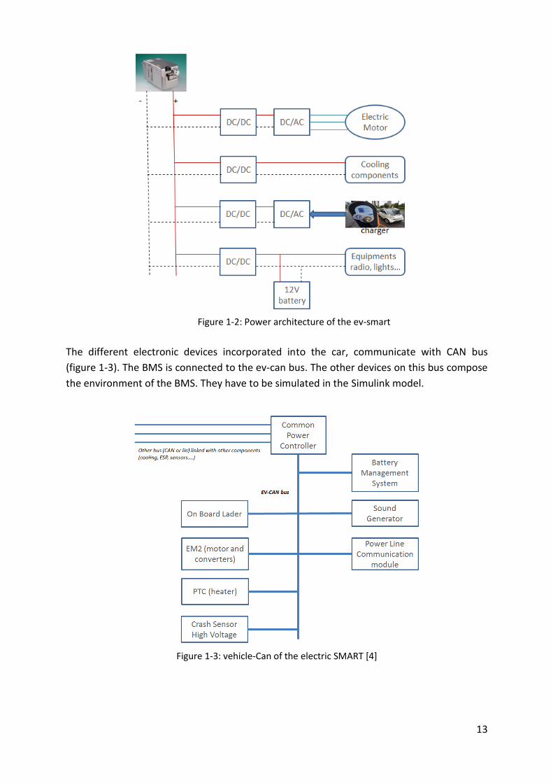
Figure 1-2: Power architecture of the ev-smart
The different electronic devices incorporated into the car, communicate with CAN bus
(figure 1-3). The BMS is connected to the ev-can bus. The other devices on this bus compose
the environment of the BMS. They have to be simulated in the Simulink model.
Figure 1-3: vehicle-Can of the electric SMART [4]

14
1.2 Lithium-ion battery
1.2.1 Main advantages and limitations
The challenge is to equip electric cars with very small batteries providing huge quantity of
energy. Presently the lithium-ion batteries are the best solution for electric cars because of
their high energy density (figure 1-4).
Figure 1-4: energy density comparison [5]
Figure 1-5 shows different operation areas for the lithium-ion cell depending on its
temperature and voltage. The temperature must stay between -10°C and 80°C and the
voltage must always be maintained between 1,8 and 4,2V. These limits are the border of the
safe area. If the cell operates in another area, it will be damaged and will lose its full
capacity.
Figure 1-5: Operation limits of lithium-ion battery [6]
To keep the battery safe, other parameters must be controlled. For example, the current
which can be drawn by the load (motor for example) during the discharge phase, must be
calculated to avoid a depth discharge (voltage under 1,8V). The same safety measure has to
be done during charging to avoid an overcharge (voltage over 4,4V).
15
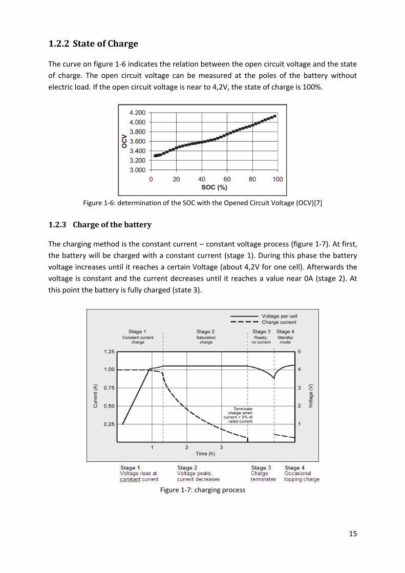
1.2.2 State of Charge
The curve on figure 1-6 indicates the relation between the open circuit voltage and the state
of charge. The open circuit voltage can be measured at the poles of the battery without
electric load. If the open circuit voltage is near to 4,2V, the state of charge is 100%.
Figure 1-6: determination of the SOC with the Opened Circuit Voltage (OCV)[7]
1.2.3 Charge of the battery
The charging method is the constant current – constant voltage process (figure 1-7). At first,
the battery will be charged with a constant current (stage 1). During this phase the battery
voltage increases until it reaches a certain Voltage (about 4,2V for one cell). Afterwards the
voltage is constant and the current decreases until it reaches a value near 0A (stage 2). At
this point the battery is fully charged (state 3).
Figure 1-7: charging process

16
1.3 Battery Management System BMS
1.3.1 BMS tasks
As explained before, all the cells of the battery have to be maintained between temperature
and voltage limits. That is the main task of the battery management system. To full fill this
task, it measures the current, voltage and temperature of the battery. Its software calculates
temperature, current, and voltage limits. If the measurements exceed the limits, the BMS
has to react.
For example, if the battery temperature is high (more than 45°C for example) the cooling
module of the BMS software has to send cooling requests to the ECU controlling the air
conditioning elements.
To determine the value of the requests, the BMS needs to know parameters from the
battery environment like the surrounding temperature or the coolant temperature. The
values are either measured by the BMS or sent by other ECUs.
Depending on the environment parameters, the value of the request is set. For instance, if
the temperature of the coolant is higher than the battery, the battery cannot be cooled by
the coolant.
Another task of the BMS is to calculate information about the battery. The BMS calculates
the state of charge of the battery or the internal resistance. These parameters are significant
for the calculation of the limits and the requests.
1.3.2 Architecture of the BMS
The hardware of the BMS (figure 1-8) is composed of the BCU, contactors, current sensor,
coolant temperature sensor, cell supervisor electronic (CSE), and a vehicle interface.

17
Figure 1-8: BMS architecture [8]
The CSE is an electronic circuit which measures temperature and voltage of each cell of the
battery. Here a CSE can only check 31 cells.
The communication between the BCU, the CSE and the other ECUs of the vehicle is
performed by CAN bus.
The current sensor measures the battery current.
The main contactors are placed on the poles of the battery to connect it, with a charge
(DC/AC converter and the motor).
The cooling water sensor measures the temperature of the cooler.
The BCU receives the information from the different sensors (current, temperature of the
coolant, voltage, battery temperature) and from the ECUs of the ev-Can bus. It performs all
the calculation (cooling requests, voltage and current limit calculation, internal resistance of
the battery).

18
2 Presentation of the way of testing
2.1 Goal of the test process
2.1.1 Principle
The purpose of the process is to test the BMS in real time with the ECUs of the ev-CAN and
the battery. The ECUs and the battery are simulated by the Simulink model.
Closing the loop (figure 2-1) enables the automatic transfer of data between the BMS and
the model.
Figure 2-1: Model and the BMS in a closed loop
2.1.2 Advantages
The real components are not needed to perform the tests, and so, they can be easily
repeated. Since the value of the sensor measurements can be overwritten, the tester can
easily set a value for a sensor and the ECU under test has to react. Special conditions (room
temperature for example) for testing are not required.
2.2 Test components
The figure 2-2 shows the architecture of the test bench. The Simulink model runs on the
real-time computer of a Hardware-In-the-Loop system (DSPACE).
The DSPACE bench provides an interface between the model and the other components of
the test bench. It transforms the BMS signals into CAN or analog signals which can be
understood by the other elements of the test bench.

19
The cell simulator simulates voltage (1 - 5V) and temperature (-40°C to 120°C) of individual
cells. 104 cells can be simulated at the same time. The cell simulator cannot provide current
(1A maximum). That is why the high voltage source is needed to simulate the global voltage
and current of the battery.
Figure 2-2: test bench
2.3 Control of the inputs/outputs of the model
2.3.1 Database with Vector CANdb++ [9]
The BMS interacts only with CAN-signals contained in CAN-messages. The messages and
their signals must be described in a database. The software Vector CANdb++ provides all the
tools needed for the creation of the database and the configuration of the CAN-
messages.Every signal has a definition, which gives the signal a name, a length, the type of
value (integer or float for example) and the values range. The signals are then set together in
CAN-messages. Every message has a name, an ID for the CAN communication, and a layout.
2.3.2 Vector CANoe and the box Vector VN8970 [10]
A CANoe simulation was used in complement to the Simulink model and was embedded in a
box called Vector VN8970.
Vector CANoe is a software which enables the simulation of can bus. In combination with
Vector CANdb++, it is possible to receive and send the CAN messages described in the
20
database. The simulation is programmed in Capl. Capl is an event programming language
designed for CANoe simulation. The Capl program determines the reaction of the nodes to
each received CAN-messages or CAN-signals.
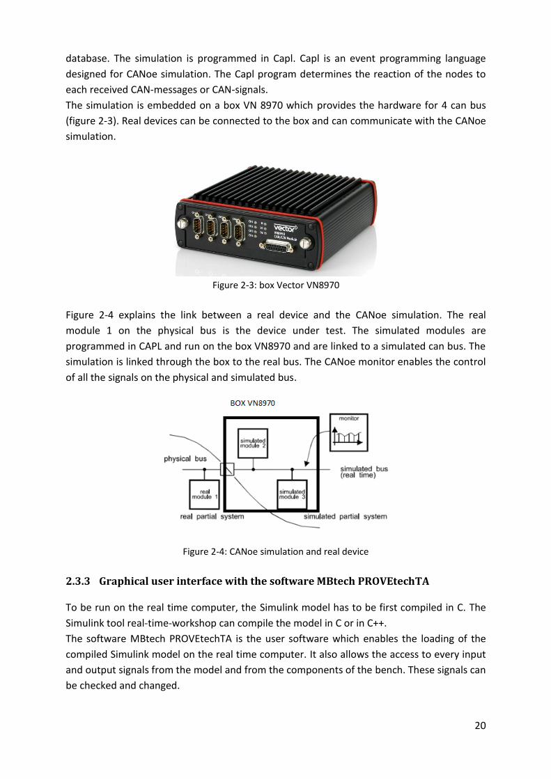
The simulation is embedded on a box VN 8970 which provides the hardware for 4 can bus
(figure 2-3). Real devices can be connected to the box and can communicate with the CANoe
simulation.
Figure 2-3: box Vector VN8970
Figure 2-4 explains the link between a real device and the CANoe simulation. The real
module 1 on the physical bus is the device under test. The simulated modules are
programmed in CAPL and run on the box VN8970 and are linked to a simulated can bus. The
simulation is linked through the box to the real bus. The CANoe monitor enables the control
of all the signals on the physical and simulated bus.
Figure 2-4: CANoe simulation and real device
2.3.3 Graphical user interface with the software MBtech PROVEtechTA
To be run on the real time computer, the Simulink model has to be first compiled in C. The
Simulink tool real-time-workshop can compile the model in C or in C++.
The software MBtech PROVEtechTA is the user software which enables the loading of the
compiled Simulink model on the real time computer. It also allows the access to every input
and output signals from the model and from the components of the bench. These signals can
be checked and changed.

21
In this PROVEtechTA screenshot (figure 2-5) some input and output signals from the model
can be seen. The signals can be changed and checked on this page.
Figure 2-5: User interface MBtechPROVEtechTA
2.4 Presentation of the model
Figure 2-6: structure of the Simulink model

22
The Simulink model is composed of 4 blocks:
- Input
- Output
- BMS_Plant
- HIL_Control
The input and output blocks configure the input and output signals. The model signals in
destination of the ev-can have to be mapped with the database. Figure 2-7 shows signals
coming from the plant model which are directed into a map block. In this block, the user
chooses the database, here the database of the ev-can, and maps the signals from the model
to the database.
Figure 2-7: mapping of signals
The HIL block configures the HIL system by setting up the control of the different bus for example.
Figure 2-8 presents a simplified view of the model structure; the common power train
controller (CPC) is responsible for the cooling/heating. The network management controls
the state (sleep, awake) of the different ECU, the on board charger provides the battery with
current, the energy management controls that the battery operate between the limits
calculated by the BMS. The cell model simulates one cell. A switch control switches between
the charge current and the discharge current.

23
Figure 2-8: overview of the plant model

24
3 Implementation of the different blocks
In this part, it is explained how the different modules are implemented. The purpose is to
understand the tasks of each ECU or function in the real car and in the simulation. The blocks
to be implemented in this thesis are the Common Powertrain Controller, the energy
management, the On Board Charger and the network management.
3.1 Common Powertrain Controller (CPC)
3.1.1 Cooling elements
This ECU is responsible for the battery cooling. It controls all the cooling components in the
car.
Figure 3-1: cooling circuits [11]
The element number 08 on figure 3-1 is called PTC, it is a heating component. It is only
activated in charge mode by a temperature less than -10°C.
The global cooling system is composed of two cooling subsystems (figure 3-1). One is
composed of water pumps (09, 10, 01) and a fan. The fan cools the coolant (water + glycol)
which circulates in the normal way of cooling circuit (figure 3-2).
25
Figure 3-2: Normal way of cooling
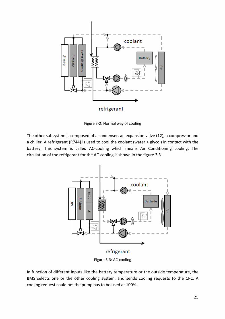
The other subsystem is composed of a condenser, an expansion valve (12), a compressor and
a chiller. A refrigerant (R744) is used to cool the coolant (water + glycol) in contact with the
battery. This system is called AC-cooling which means Air Conditioning cooling. The
circulation of the refrigerant for the AC-cooling is shown in the figure 3.3.
Figure 3-3: AC-cooling
In function of different inputs like the battery temperature or the outside temperature, the
BMS selects one or the other cooling system, and sends cooling requests to the CPC. A
cooling request could be: the pump has to be used at 100%.
26
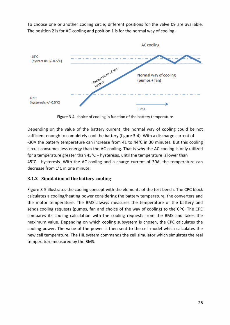
To choose one or another cooling circle; different positions for the valve 09 are available.
The position 2 is for AC-cooling and position 1 is for the normal way of cooling.
Figure 3-4: choice of cooling in function of the battery temperature
Depending on the value of the battery current, the normal way of cooling could be not
sufficient enough to completely cool the battery (figure 3-4). With a discharge current of
-30A the battery temperature can increase from 41 to 44°C in 30 minutes. But this cooling
circuit consumes less energy than the AC-cooling. That is why the AC-cooling is only utilized
for a temperature greater than 45°C + hysteresis, until the temperature is lower than
45°C - hysteresis. With the AC-cooling and a charge current of 30A, the temperature can
decrease from 1°C in one minute.
3.1.2 Simulation of the battery cooling
Figure 3-5 illustrates the cooling concept with the elements of the test bench. The CPC block
calculates a cooling/heating power considering the battery temperature, the converters and
the motor temperature. The BMS always measures the temperature of the battery and
sends cooling requests (pumps, fan and choice of the way of cooling) to the CPC. The CPC
compares its cooling calculation with the cooling requests from the BMS and takes the
maximum value. Depending on which cooling subsystem is chosen, the CPC calculates the
cooling power. The value of the power is then sent to the cell model which calculates the
new cell temperature. The HIL system commands the cell simulator which simulates the real
temperature measured by the BMS.

27
Figure 3-5: simplified process of cooling
3.1.3 CPC Simulink block implementation
3.1.3.1 Functions of the CPC
The global objective was at the beginning, to make possible in the model, the cooling of the battery with the 2 ways of cooling (AC-cooling and cooling with pumps and fan), add a heating function and add output signals to test deeper functions of the software.
3.1.3.2 Important input signals
<PNHV_CoolInletTemp> is the temperature of the coolant before being in contact with the
battery.
<PNHV_TM_WtrPmp_Rq> is a request (%) for the Water pump. It is calculated in function of
the temperature of the battery.
<PNHV_TM_Fan_Rq> is a request (%) for the fan. It is calculated in function of the
temperature of the battery.
<PNHV_SwVlv_Stat> is one of the 2 signals responsible for the choice of cooling system. It is
the status signal of the valve 09 which links the 2 cooling circles.
<PNHV_SupBat_Cool_Rq>is the second signal responsible for the choice of cooling system.
The BMS sends this request to cool the battery with AC-cooling.
<PNHV_HVAC_Comp_Speed_Rq> is the compressor speed request
These signals are sent by the BMS. CPC will use these signals in order to calculate the needed
cooling power, and to choose a way of cooling.
<DCDC_Temp> is the DCDC converter temperature
<EM_Temp> is the electromotor temperature
3.1.3.3 Output signals
<VCANR_Therm_CoolMode_Stat> different modes are distinguished. Predrive mode, drive
mode, charge mode. The BMS is only activated in drive or in charge mode.
<Therm_CoolInletTemp> is the temperature of the coolant after flowing out the battery.

28
<Therm_PNHV_WtrPmp_Req> is a request for the water pump, if the temperature of the
battery is smaller than -10°C.
<Therm_PNHV_CoolMode_Rq> is 1 if the PTC (heat element) has to be activated.
<P_Gen.cool_out> is the global power for the entire battery.
<Therm_Wtr_Pmp_Stat> is the status of the water pump.
<Therm_Fan_Stat> is the status of the fan.
<PNHV_Evap_CoolVlv_Rq_HVAC> is the request for the valve 12, and must be one (close) if
the BMS chooses the AC-cooling.
<CompSpd_V2> represents the speed of the compressor (%).
<AirTemp_Outsd> is the outside temperature.
<HVAC_Ref_Circ_NA> indicates if the AC-cooling is possible.
<VehSpd_Disp> is the speed of the vehicle.
<Therm_SwVlv_Stat> is the status of the valve 03.
<HVAC_CoolCirc_Actv> indicates if the cooling for the cabin is running.
<AirTemp_Outsd_Qual> indicates if the measured temperature is the exact value or a
modulated value.
<PNHV_BMS_Cool_Rq> is a signal to indicate that the battery is cooled by itself.
<P_Batt_out> is the by the BMS calculated cooling power for one cell. The cell block will use
this power to calculate the temperature of the battery.
3.1.3.4 Outside Temperature signal
This signal is important, because it is involved in the determination of the cooling requests.
The BMS measures the battery temperature and compares it with the temperature of the
coolant, and with the outside temperature. The BMS decides in function of the comparisons
if the battery can be cooled and which cooling circuit must be used.
3.1.4 Implementation
3.1.4.1 Power calculation test
The power calculation was already implemented by the former student but it has to be
tested. In this part, it is explained how the power is calculated, in order to understand the
tests on the power in the next part.
As said before, the cooling elements have to be controlled by the CPC. The requests sent to
these elements are percentage. 100% means that 100% of the element power is necessary.
The requests from the BMS to the CPC only concern the cooling of the battery, whereas the
requests of the CPC also concern the cooling for power electronic components.
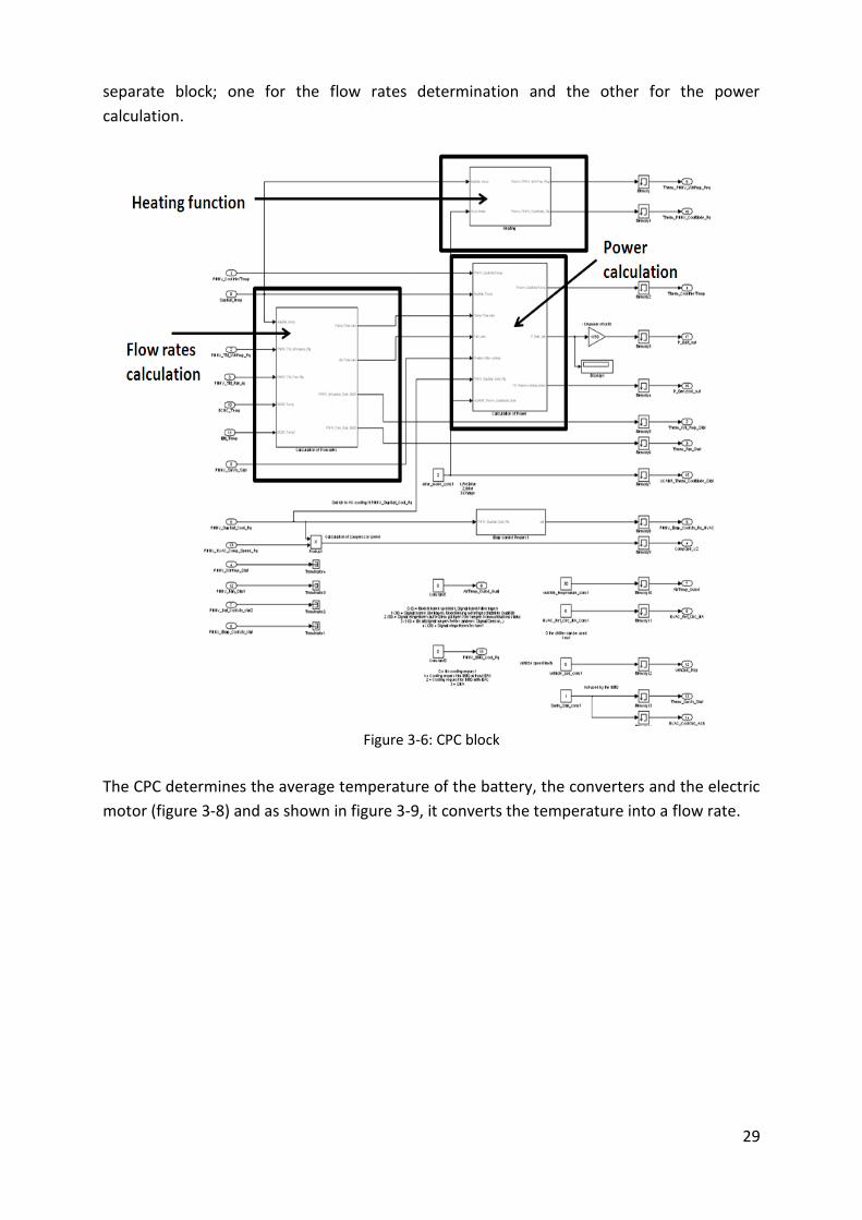
The calculation of the power is divided in 2 main parts (figure 3-7). The first one will
determine with the requests from the BMS, the flow rates (air and pump). The second part
takes in account these flow rates to calculate the power. Each part is implemented in a
29
separate block; one for the flow rates determination and the other for the power
calculation.
Figure 3-6: CPC block
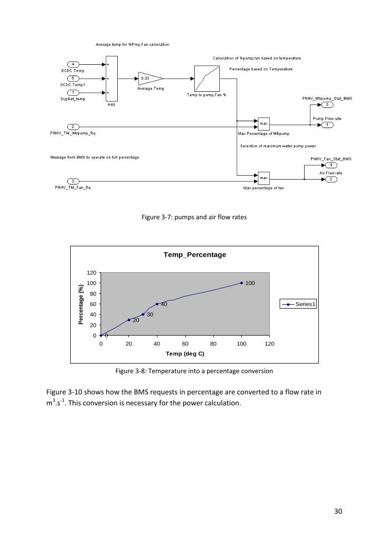
The CPC determines the average temperature of the battery, the converters and the electric
motor (figure 3-8) and as shown in figure 3-9, it converts the temperature into a flow rate.
30
Figure 3-7: pumps and air flow rates
Figure 3-8: Temperature into a percentage conversion
Figure 3-10 shows how the BMS requests in percentage are converted to a flow rate in
m3.s-1. This conversion is necessary for the power calculation.
Temp_Percentage
0
2030
40
100
0
20
40
60
80
100
120
0 20 40 60 80 100 120
Temp (deg C)
Perc
en
tag
e (
%)
Series1

31
Figure 3-9: determination of air flow rate table
The main formula to calculate the power is:
- ΔT K
- Density kg.m-3
- Flow rate m3.s-1
- Specific heat J.kg-1.K-1
- P W
For the normal way of cooling, the coolant is a water and glycol mix in ration 50:50. Its
properties are:
- Density 1080 kg.m-3 - Specific Heat Capacity 3320 J.kg-1.K-1
For the AC-cooling the refrigerant is R-744.
- Density 1839 kg.m-3 - Specific Heat Capacity 3380 J.kg-1.K-1
For the AC-cooling, it is assumed that the cooling power provided to the battery is always
the same. For the normal way of cooling the flow rates are needed. The ΔT involved in the
calculation is the difference between the coolant temperature before being in contact with
the battery and after, as shown in figure 3-10.

32
Figure 3-10: temperature of the coolant exchange
If the battery is cooled, Tcoolant_Out must be greater than Tcoolant_In. The difference in
temperature Tcoolant_Out and Tcoolant_In is utilized to calculate the cooling power for the normal
way of cooling, as presented in figure 3-11.
Figure 3-11: Cooling Power calculation (normal way of cooling)
A switch was added: if Tcoolant_in is higher than Tcoolant_out, the power is negative and the
battery is heated. The switch block avoids the heating power, because it was preferred to
have a special block for the heating function. The power coming from the fan is added to this
calculated value.
3.1.5 Choice of power
The CPC model can provide 2 cooling powers (one for the AC-cooling and one for the normal
way of cooling) and a heating power. In the block responsible for the power calculation, a
block called choice of cooling system (figure 3-13) controls the choice of the cooling circuit.
This is an embedded Matlab program. It controls with its output signal y, the multiplexer.
If y = 1, the power is 0W. If y = 2 the power is the AC-cooling power, y=3 is the normal way of
cooling and y = 4 is for the heating power.

33
Figure 3-12: Choice of the power
To choose the cooling subsystem, the following conditions have to be taken in account:
- The cooling powers are only available in the drive and charge mode.
- For using the normal way of cooling, the valve 09 has to be on position one.
- For using the AC-cooling the valve 09 has to be on position 2 and the CPC has to receive a
special request from the CPC (PNHV_SupBat_cool_Rq).
-In addition in the charge mode, if the temperature is less than -10°C, the CPC provides a
constant heating power.
To implement the embedded Matlab code for choosing the way of cooling, a truth table
(figure 3-14) was elaborated. The signal PNHV_SupBat_cool_rq is a signal from the BMS,
which means that the battery needs AC-cooling.
INPUTS OUTPUTS
PNHV_SwVlv_stat PNHV_SupBat_cool_rq Power PNHV_Evap_CoolVlv_Rq_HVAC
POS2 0 0 Open
POS2 1 AC Close
POS1 0 C Open
POS1 1 AC Close
Figure 3-13: inputs and outputs for the charging and drive mode
34
AC: Air conditioning
C: normal way of cooling
0: no cooling
The last case does not happen. PNHV_SwVlv_stat should change to POS2 before having
PNHV_SupBat_cool_rq = 1.
In the charging mode, if the battery temperature is above -10°C, it was decided that the CPC
provides a 500W heating power.
The messages sent to the BMS are:
Therm_PNHV_WtrPmp_Req = 100%
Therm_PNHV_CoolMode_Rq = 1
For all the other cases the output power is 0W!
3.1.6 Test of the power calculation
The objective was not to get the real power, but to approximate its behaviour and to cool
the battery with the 2 ways of cooling. From the study of the power calculation, points to be
verified were decided and the input signals were chosen in consequence and the CPC
outputs were checked.
3.1.6.1 Scenario 1
The points to be verified are: Does the cooling power increase if the BMS requests are
stronger. Does the CPC make the comparison between the requests from the BMS and its
own values?
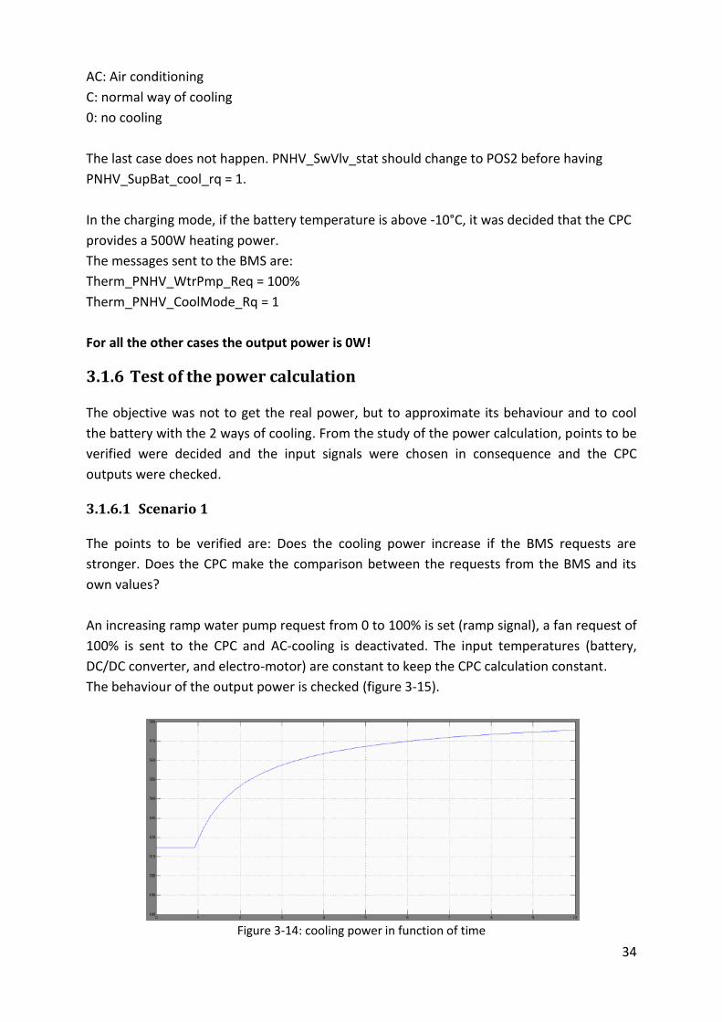
An increasing ramp water pump request from 0 to 100% is set (ramp signal), a fan request of
100% is sent to the CPC and AC-cooling is deactivated. The input temperatures (battery,
DC/DC converter, and electro-motor) are constant to keep the CPC calculation constant.
The behaviour of the output power is checked (figure 3-15).
Figure 3-14: cooling power in function of time

35
At the beginning the cooling power is constant. This is normal because the BMS pump
request is lower than the pump calculation of the CPC. At first the BMS pump request has no
influence on the calculation. As soon as it becomes greater than the percentage of the pump
request from the CPC, the CPC takes the BMS requests for the flow rate used for the power
calculation.
To sum up, the CPC compares its calculation with the request form the BMS and the cooling
power increase with the increase of the BMS request. That is a correct behaviour.
3.1.6.2 Scenario 2
It has to be verified if the normal way cooling power rises if the temperatures in input
increases.
The requests of the BMS are set to 0% and the AC-cooling is deactivated. An increasing
ramp was given for the temperature of the DC/DC converter.
Figure 3-15: cooling power in W in function of time
As a result, an increasing power was obtained for an increasing converter temperature.
The power increases if the temperature of the power components goes up.
3.1.6.3 Scenario 3
The aim of this scenario is to check if the CPC calculates a higher value of cooling power if
the battery temperature increases.
The requests of the BMS are 100% in order to have a constant influence on the calculation of
power. The AC-cooling is not used. The input temperature of the coolant is constant (30°C).
Since the input temperature of the coolant is constant and the temperature of the battery
goes up, the output temperature of the coolant increases as well. This is because the battery
gives more and more heat to the coolant. As a result the cooling power should increase as
well because of the ∆T from the power calculation: Tcoolant_out – Tcoolant_in.
36
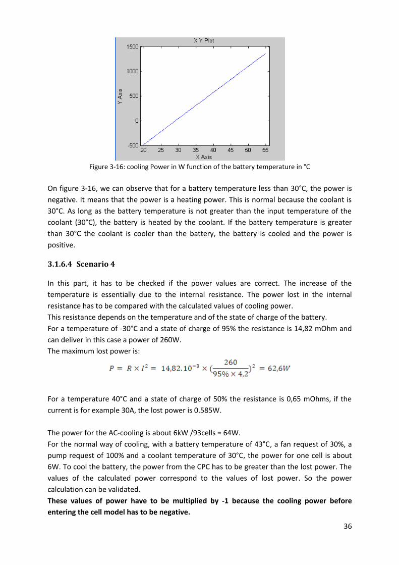
Figure 3-16: cooling Power in W function of the battery temperature in °C
On figure 3-16, we can observe that for a battery temperature less than 30°C, the power is
negative. It means that the power is a heating power. This is normal because the coolant is
30°C. As long as the battery temperature is not greater than the input temperature of the
coolant (30°C), the battery is heated by the coolant. If the battery temperature is greater
than 30°C the coolant is cooler than the battery, the battery is cooled and the power is
positive.
3.1.6.4 Scenario 4
In this part, it has to be checked if the power values are correct. The increase of the
temperature is essentially due to the internal resistance. The power lost in the internal
resistance has to be compared with the calculated values of cooling power.
This resistance depends on the temperature and of the state of charge of the battery.
For a temperature of -30°C and a state of charge of 95% the resistance is 14,82 mOhm and
can deliver in this case a power of 260W.
The maximum lost power is:
For a temperature 40°C and a state of charge of 50% the resistance is 0,65 mOhms, if the
current is for example 30A, the lost power is 0.585W.
The power for the AC-cooling is about 6kW /93cells = 64W.
For the normal way of cooling, with a battery temperature of 43°C, a fan request of 30%, a
pump request of 100% and a coolant temperature of 30°C, the power for one cell is about
6W. To cool the battery, the power from the CPC has to be greater than the lost power. The
values of the calculated power correspond to the values of lost power. So the power
calculation can be validated.
These values of power have to be multiplied by -1 because the cooling power before
entering the cell model has to be negative.

37
3.2 Cell-model
The cell-model (figure 3-17) was already implemented by Deutsche ACCUmotive.
The output signal of this block controls the cell simulator. It will command the temperature
of the cells, their voltage, and the global voltage of the battery. In this thesis, the model was
only utilized to perform the tests.
Figure 3-17: cell model
To use this model, the initial conditions have to be first determined (initial temperature,
Start SOC is the initial State of charge).
Zeit is the integration time used in the model for calculation.
Strom is the current. If the current is positive, it is a charge current, if not it is a discharge
current.
P_Kühlung is the power which comes from the CPC module. If the Power is negative the
power is a cooling power.
The output temperature and the cell voltage are the output values which will be sent to the
BMS. The other outputs allow us to compare the calculated values and the values measured
by the BMS.
P_Wärme_Bilanz_Zelle is the global power which comes from the losses, from the current
and the cooling module.
The global voltage of the battery is approximated by multiplying the cell voltage by the
number of cells (93 for the electric smart “fortwo”).
3.3 Network management (NM)
The task of this module is to control the states of the ECUs. They can be off, they can sleep
or participate in the communication. The different states are necessary in the car for saving
energy. The protocol used in the smart “fortwo” is the protocol OSEK, but this module was
also implemented with the protocol AUTOSAR.
38
3.3.1 Protocol OSEK [12]
3.3.1.1 Theory
The OSEK NM communication was implemented by a consortium of automotive companies
like Daimler AG and BMW. The purpose was to create a standard communication protocol in
order to simplify the communication between the different electronic control units (ECUS)
coming from many producers.
Each node or ECU has communication modes. It can be awaken (awake mode or ring mode),
in a bus sleep mode or in an error mode (limphome). To communicate at each other, they
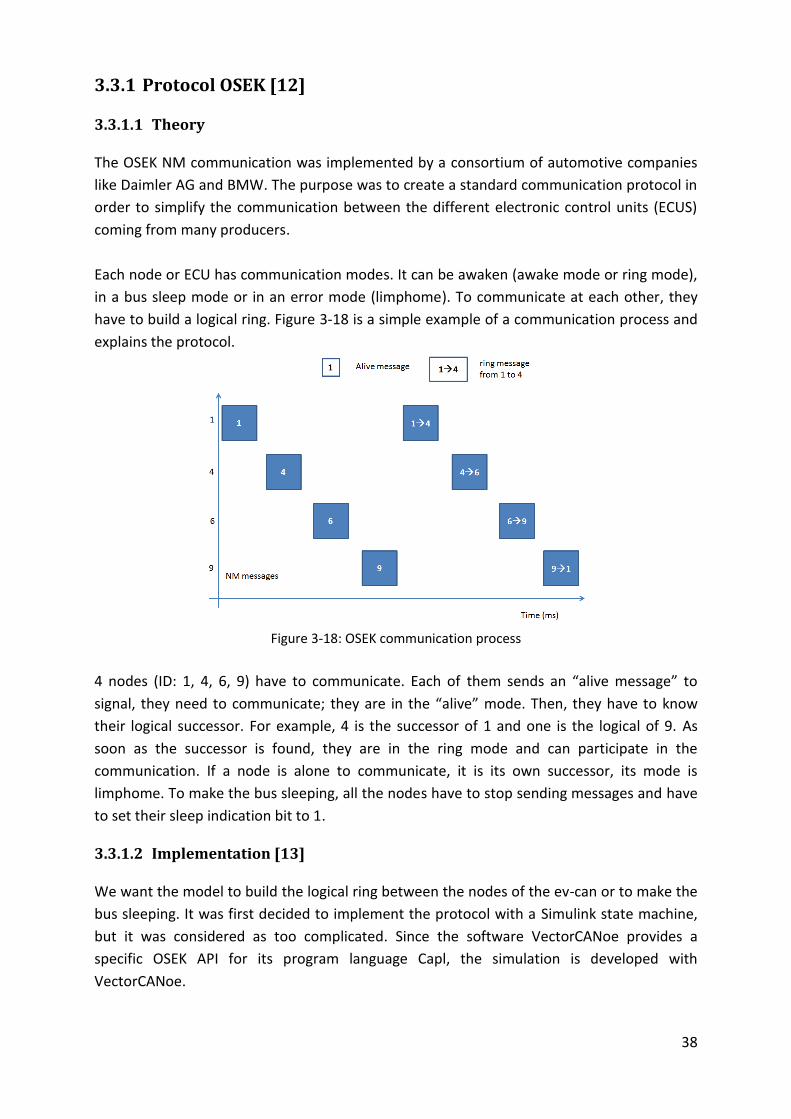
have to build a logical ring. Figure 3-18 is a simple example of a communication process and
explains the protocol.
Figure 3-18: OSEK communication process
4 nodes (ID: 1, 4, 6, 9) have to communicate. Each of them sends an “alive message” to
signal, they need to communicate; they are in the “alive” mode. Then, they have to know
their logical successor. For example, 4 is the successor of 1 and one is the logical of 9. As
soon as the successor is found, they are in the ring mode and can participate in the
communication. If a node is alone to communicate, it is its own successor, its mode is
limphome. To make the bus sleeping, all the nodes have to stop sending messages and have
to set their sleep indication bit to 1.
3.3.1.2 Implementation [13]
We want the model to build the logical ring between the nodes of the ev-can or to make the
bus sleeping. It was first decided to implement the protocol with a Simulink state machine,
but it was considered as too complicated. Since the software VectorCANoe provides a
specific OSEK API for its program language Capl, the simulation is developed with
VectorCANoe.
39
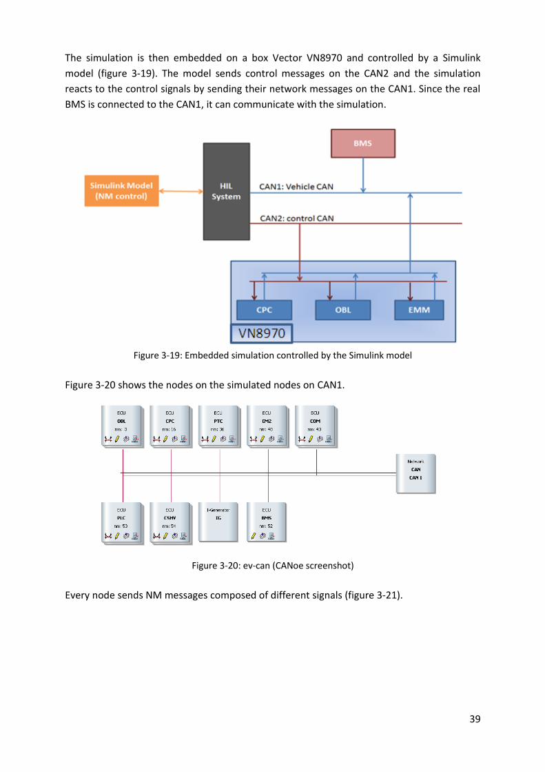
The simulation is then embedded on a box Vector VN8970 and controlled by a Simulink
model (figure 3-19). The model sends control messages on the CAN2 and the simulation
reacts to the control signals by sending their network messages on the CAN1. Since the real
BMS is connected to the CAN1, it can communicate with the simulation.
Figure 3-19: Embedded simulation controlled by the Simulink model
Figure 3-20 shows the nodes on the simulated nodes on CAN1.
Figure 3-20: ev-can (CANoe screenshot)
Every node sends NM messages composed of different signals (figure 3-21).

40
Figure 3-21: NM message from OBL called NM_OBL and its signals
A node (OBLwith its Id = 03 for example) sends an Alive message: NM_Successor = 03 and
NM_Mode = Alive. We assumed that the logical successor is CPC with its ID = 16. Then in the
next message sent by OBL, NM_Successor = 16 and NM_Mode = Ring. To enter the bus sleep
mode, each node of the ring has to send NM_Sleep_ind = 1, then one node sends
NM_Sleep_Ack = 1 and all the nodes sleep.
To control the simulation, the command message enables the Capl program of each node to
change their sleep indication (figure 3-23).
Figure 3-22: command message (VectorCANdb++)
For example, the node OBL has to communicate, the model sends the command message
with Enable_OBL= 1 and Sleep_ind_OBL = 0. The Capl program of the OBL starts the OSEK
simulation of OBL because of the signal Enable_OBL and sets the sleep indication bit to 0.
2 Simulink models were implemented.
In the first one, only the node CPC and OBL were simulated. Each of them can be controlled
individually. It was chosen to have an enable request and a sleep_indication request for
every node. A button cl15 set all the sleep indication to 1 or 0. This allows waking up in one
time all the simulated nodes or sending all of them in the sleep mode.

41
The second one has to react to the BMS signal. The aim is to wake up one node, the BMS
reacts, and the other nodes react after the BMS.
The Simulink model was implemented with a state machine for each node.
Figure 3-23: Simulinkstate machine for one node
First all the ECUs are sleeping, init = 0, and have their sleep_ind equals to 1. The user wakes
up one node by setting its sleep_ind to 0. The state changes to AwakeByCommand. The BMS
wakes up and change its sleep_ind to 0. This makes the other nodes waking up, because of
the condition Sleep_Ecu_Rq ~= 0 AND Sleep_Ind_BMS==0.
Then the user sets init = 1, if the BMS has its sleep_ind set to 1. All the ECUs enter the bus
sleep mode. Without the init variable, the ECUs would not be stopped in the state
AwakeByCommand.
3.3.2 AUTOSAR
Like OSEK, AUTOSAR was developed together by many companies like Daimler, Ford or PSA.
The AUTOSAR network management is an evolution of OSEK. The purpose is to build an
architecture allowing developers to implement software without thinking about the
hardware.
The network is implemented as a states-machine. There are 3 main states: running, waiting
and suspended [15]. In the running state, the ECU sends and receives messages. If no task
has to be performed, the ECU switches to the waiting state. In this state, it only receives
messages. If no message is received, this means that the other nodes are either in the
waiting state or in the suspended mode. If all the nodes are in the waiting mode, they all
switch to the suspended mode. The simulation was implemented like the OSEK simulation
with the software CANoe.
42
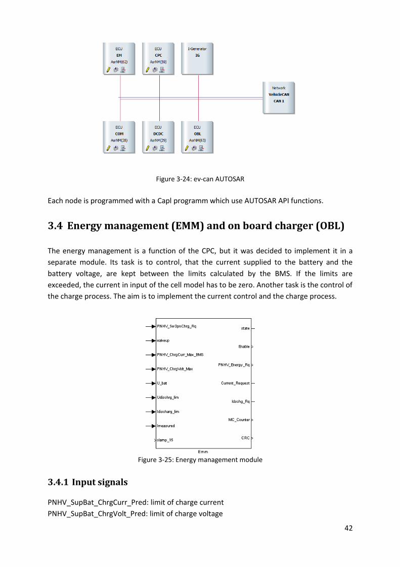
Figure 3-24: ev-can AUTOSAR
Each node is programmed with a Capl programm which use AUTOSAR API functions.
3.4 Energy management (EMM) and on board charger (OBL)
The energy management is a function of the CPC, but it was decided to implement it in a
separate module. Its task is to control, that the current supplied to the battery and the
battery voltage, are kept between the limits calculated by the BMS. If the limits are
exceeded, the current in input of the cell model has to be zero. Another task is the control of
the charge process. The aim is to implement the current control and the charge process.
Figure 3-25: Energy management module
3.4.1 Input signals
PNHV_SupBat_ChrgCurr_Pred: limit of charge current
PNHV_SupBat_ChrgVolt_Pred: limit of charge voltage

43
PNHV_SupBat_DschrgCurr_Pred:limit of discharge current
PNHV_SupBat_DschrgVolt_Pred: limit of discharge voltage
PNHV_SwOpnChrg_Rq is a signal sent by the BMS when the battery is full charged.
Wake up is a signal sent by the charger when the user plugs the power supply.
Clamp 15 is a signal which comes from the HIL system to control manually the contactors.
Imeasured is the real current flowing out or in the battery. It is simulated by the high voltage
source and measured by the BMS. The model has access to it.
3.4.2 Output signals
Current_Request is the current request to the charger by charging.
Idsch_Rq is the current flowing out the battery if the battery is discharged.
MC_Counter and CRC are specific signals for the check sum of a CAN bus.
PNHV_Energy_Rq is a signal sent to the BMS it commands the contactors allowing the
connection between the battery and the power source or the last.
3.4.3 Power prediction from the BMS
The aim of the power prediction is to calculate the maximum power the system can take or
consume in respect with the current and voltage limits. These limits are calculated by the
BMS. The algorithms take in account different parameters like the temperature and the
internal resistance. Deutsche ACCUmotive performed tests and sketched different curves to
find the current and voltage limits. The discharge and charge current limits are determined
for example in function of the temperature.
This is the algorithm used during the charge:
if (OCV + (I_max_ch*Ri) <U_max_ch)
{
I_pred_ch= I_max_ch;
U_pred_ch= (OCV+(I_max_ch*Ri));
}
else if (OCV + (I_max_ch*Ri) >U_max_ch)
{
U_pred_ch= U_max_ch;
I_pred_ch= (U_max_ch - OCV)/Ri;
}
The battery is first charged with a high constant current (I_max_ch). In consequence, the
voltage of the battery increases from U_min_disch to OCV + (I_max_ch*Ri) >U_max_ch. At
this point the OCV is about to reach its maximum value and the charge current has to
decrease in order to not overcharge the battery. At the end, OCV = U_max_ch and the
charge current is 0A.

44
During discharge:
if (OCV - (I_max_disch*Ri) >U_min_disch)
{
I_pred_disch= I_max_disch;
U_pred_disch= U_min_disch - (I_max_disch*Ri);
}
Elseif (OCV - (I_max_disch*Ri) <U_min_disch)
{
U_pred_disch= U_min_disch;
I_pred_disch= (OCV - U_min_disch)/Ri;
}
The battery can be discharged with the maximum current until the OCV voltage reaches the
minimum allowed voltage. When the battery is completely discharged, OCV = U_min_disch
and the discharge current has to be 0A.
The limits I_max_disch and I_max_ch depend on the operating temperature and we want
the limits to depend on the open circuit voltage and on the internal resistance. That is why;
it was decided to take the prediction values rather than I_max_disch and I_max_ch.
3.4.4 Structure of the module
Figure 3-26: structure of the energy management module
The main contactors connect the battery to its load or to the power source. They can be
controlled either manually by cl15 or by the state machine.
45
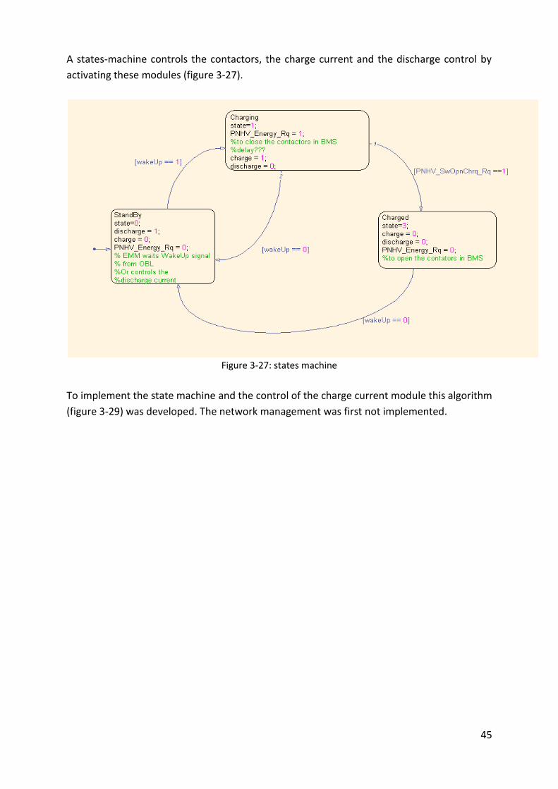
A states-machine controls the contactors, the charge current and the discharge control by
activating these modules (figure 3-27).
Figure 3-27: states machine
To implement the state machine and the control of the charge current module this algorithm
(figure 3-29) was developed. The network management was first not implemented.
46
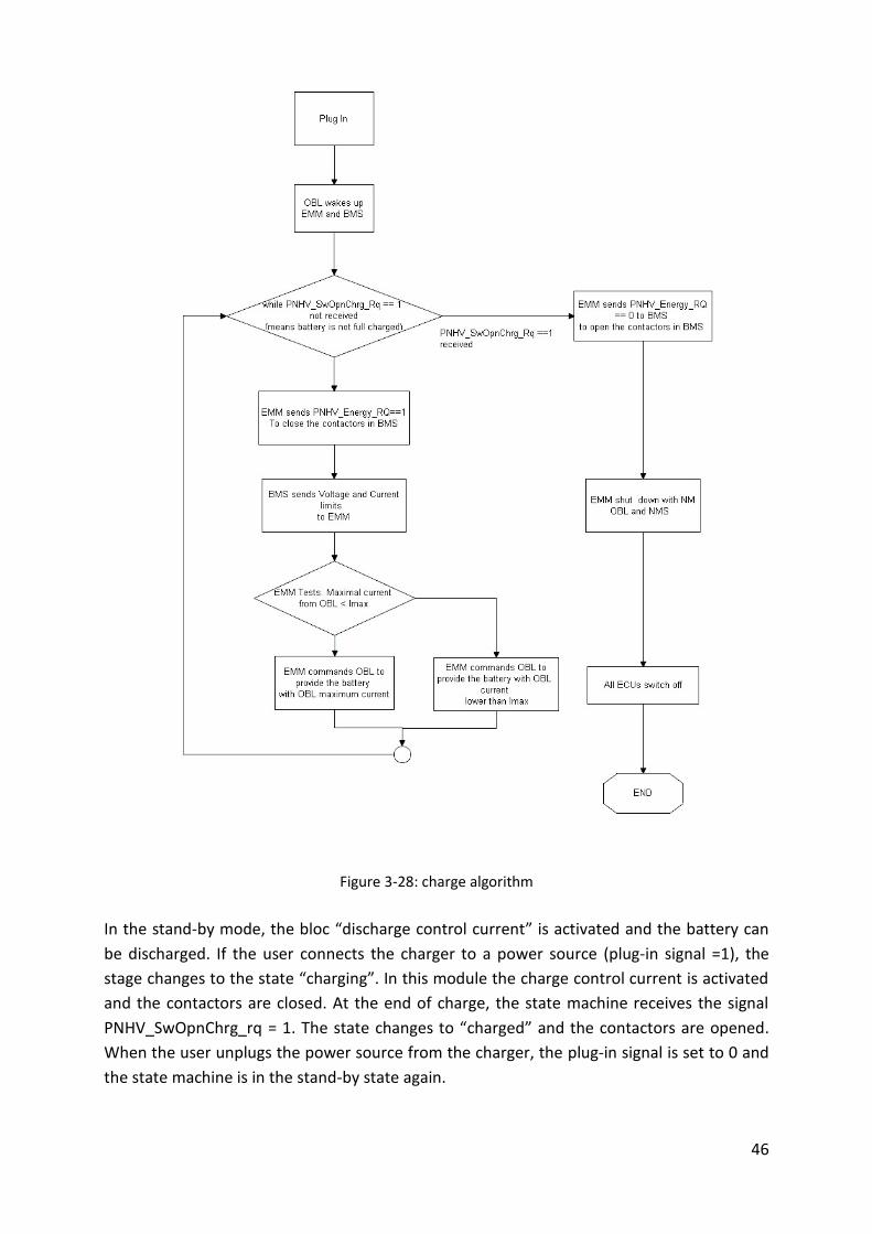
Figure 3-28: charge algorithm
In the stand-by mode, the bloc “discharge control current” is activated and the battery can
be discharged. If the user connects the charger to a power source (plug-in signal =1), the
stage changes to the state “charging”. In this module the charge control current is activated
and the contactors are closed. At the end of charge, the state machine receives the signal
PNHV_SwOpnChrg_rq = 1. The state changes to “charged” and the contactors are opened.
When the user unplugs the power source from the charger, the plug-in signal is set to 0 and
the state machine is in the stand-by state again.

47
The task of the charge current control module is to send the current request to the charger.
It compares the maximal current which can be provided by the charger with the maximal
charge current limit sent by the BMS. If the current limit is higher than the maximal OBL
current, the request is the OBL maximum current. If not, the request is the current limit from
the BMS minus 3 Amperes. When the current limit reaches 0A, the current request from the
emm is 0A (figure 3-29).
Moreover this block checks the current flowing in the battery. It can happen that the flowing
current is different from the request current. So if the current flowing in the battery is
greater than the limit, the request is set to zero. Another solution should be to open the
contactors.
Figure 3-29: Charge current request
The task of the discharge control current is to control that the discharge current is always
under the maximum discharge current limit, and avoid depth discharge. If the limits are
exceeded, the current is changed to 0A.
3.5 On board charger
In the real car, the charger provides the battery with current, and wakes up the other signal
as soon as a power source is plugged. The current from OBL has to follow the current
request from the EMM. It also sends a signal to the BMS, to indicate the mode it is
operating. The charger may need a current regulation if the battery current value in the
model is not the same as the current measured by the BMS.

48
4 Tests
The tests were performed in the Simulink environment and on the HIL bench. For the offline
tests in the Simulink environment, a model was created with a BMS model. The cooling
functions and the limits calculation were implemented in the BMS model according to the
different test scenarios. The aim is to perform the following scenarios and to check, if the
implementation of the plant model is correct.
Figure 4-1: Simulink model for offline tests
The OCV of one cell is multiplied by 93 inside the battery block.
The tests are performed on the HIL test bench, to check:
- if the model can be compiled
- if the compiled model behaves like the Simulink model
- if the model interact with the BMS
- the reaction of the BMS
4.1 Cooling module
4.1.1 Scenarios
The BMS activates the normal method of cooling if:
- the temperature of the battery is between 40 and 45°C

49
- the temperature of the coolant (PNHV_coolInletTemp) < 44°C and lower than the battery
temperature.
- the car mode is drive or charge (VCANR_Therm_CoolMode_stat = 2 for drive or 3 for
charge)
- the outside temperature (AirTemp_Outsd) < 30°C
- The position of the valve for switching the way of cooling is 01 (PNHV_SwVlvStat = 1)
During 900s, the request coming from the BMS should be:
- Water pumps 100% (PNHV_TM_WtrPmp_Rq)
- Fan 40% (PNHV_TM_Fan_Rq)
The cooling continues if the coolant is kept 6°C lower than the battery temperature.
If the battery temperature is greater than 45°C (hysteresis +/- 0,5°C) AND AC-cooling is
notavailable (HVAC_Ref_Circ_NA = 1), the requests from the BMS should be:
- Water pumps 100% (PNHV_TM_WtrPmp_Rq)
- Fan 100% (PNHV_TM_Fan_Rq)
If these conditions are not filled, then there is no cooling.
The BMS activates the AC-cooling if:
- the battery temperature is over 45°C
- the AC-cooling can be activated (HVAC_Ref_Circ_NA = 0)
- the position of the valve for switching the cooling circuit is POS2 (PNHV_SwVlvStat = 2)
The request should be:
- PNHV_SupBat_cool_Rq = 1
For the heating function, the battery temperature has to be lower than -10°C and the mode
has to be “charge”.
The requests have to be:
- Therm_PNHV_WtrPmp_Req = 100%
- Therm_PNHV_CoolMode_Rq = 1
These conditions were implemented in a Simulink BMS model to perform the tests in the
Simulink environment in a closed loop. To test the different functions of the cooling BMS
cooling software, the outputs of the CPC have to be adapted to these conditions.

50
4.1.3 Offline test
Figure 4-2 is an example of a cooling with a 100A discharge. First the battery temperature is
44°C, the fan request is 40% and the pump request is 100%. Since the cooling power is not
sufficient enough, the temperature increases until it reaches 45,5°C. Here, the BMS chooses
the AC-cooling (PNHV_SupBat_Cool_Rq = 1 and PNHV_SwVlv_Stat = 2). The temperature
decreases until 44,5°C. Then the BMS chooses the normal way of cooling again and the cycle
continues.
Figure 4-2: cooling with a -100A discharge current
4.1.4 Online Test
It was first important, to check if the compiled model behaves like the Simulink model.
Inputs were chosen according to the truth table defined in the paragraph 3.1.4 and the
output power was checked. Then, the battery temperature was changed manually in order
to get the different cooling requests from the BMS. Lower than 40°C the fan and the pump,
the pump and fan requests were 0%. Between 40 and 45 °C the pump request was 100% and
the fan request was 30%. More than 45°C the requests were 100%, but the request for

51
AC-cooling was not sent. So the model behaves like the Simulink model but the interaction
with the BMS has to be further studied, to have the same interaction as in the car.
4.2 Energy management and on board charger module
4.2.1 Scenarios
To test the charge process, the plug_in signal from OBL has to be set to 1. The EMM must
send the signal for closing the contactors (PNHV_energy_Rq = 1) to the BMS. The current
from the OBL to the battery has to follow the request of the EMM. The battery must be
charged according to the constant-current /constant-voltage process. The signal indicating
the end of charge has to be sent by the BMS. The EMM must open the contactors. When the
signal called plug-in = 0, it has to be checked if the contactors can be closed with cl15 and if
the battery can be discharged. By discharging, the current has to be maximal until the
voltage reaches its minimal value.
4.2.2 Offline tests
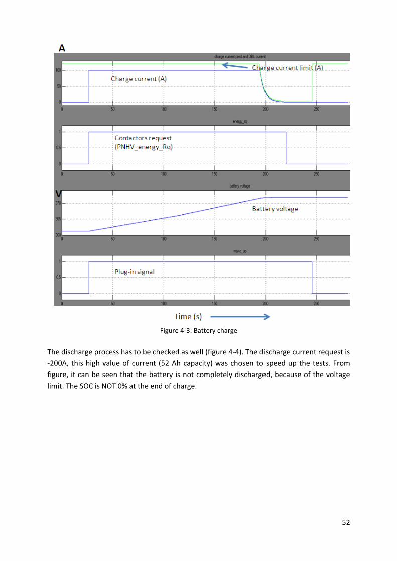
The charge process is checked in figure 4-3. The signal plug-in = 0 means that the OBL is not
plugged to a power source and the energy request must be 0. So, the contactors are opened
and the current flowing in the battery is 0A. Then the charger is plugged and the current
flowing in the battery follows the current limits. At the end of the charge, the contactors are
closed and no current flows in the battery. The charge process is correct and can be tested
with the real BMS on the HIL test bench.
52
Figure 4-3: Battery charge
The discharge process has to be checked as well (figure 4-4). The discharge current request is
-200A, this high value of current (52 Ah capacity) was chosen to speed up the tests. From
figure, it can be seen that the battery is not completely discharged, because of the voltage
limit. The SOC is NOT 0% at the end of charge.

53
Figure4-4: complete discharge and partial charges/discharges
4.2.3 Online tests
The tests were performed on the HIL bench with the BMS of the smart “fortwo electric
drive”. The software PROVEtechTA loads the compiled Simulink model, and enables the
tester to check and change manually the signals he wants. The state machine was first
tested. The wake up was first set to 0, then to 1. Afterward the signal of end of charged was
set to 1. The variable “state” from the state machine indicates the stages of the process. The
state machine behaves like the Simulink model according to the offline tests. It reacts to the
wake up signal and to the end of charge signal.
The second thing to test is: does the current from OBL follow the limits of the BMS.
To perform the test, Plug_in signal is set to1. To speed up the tests, the voltage of the cells
was changed manually changed from 3V to 4,3V. The state of charge and the current were
checked.

54
Figure 4-5: charge current limits test
The BMS calculates limits according to constant current–constant voltage process, and the
OBL provides the battery with current according to the limits from the BMS. The limit near
from the end of charge increases and the signal of end of charge is not sent. This is because
the mode from OBL was not sent and the tests were stopped too early. The signal comes 30s
after these conditions are filled:
- Cell voltage > 4,19V
- Current < 2,5A
4.3 Network management
4.3.1 OSEK
In order to simplify for this document, the tests were only performed with 2 nodes (CPC and
OBL).
4.3.1.1 Offline tests
The Simulink model and the CANoe simulation have to run on a computer. It has to be
tested, if the nodes can be enabled, if they can enter the sleep_mode anf if they can build a
ring. A command signal is sent with Simulink, and it is checked, if the command signal arrives
on the bus and if the programmed node answers.
Figure 4-6, a ring is built between the OBL and the CPC. They are in ring mode (253),
NM_successor of OBL is 16 which is the ID of the CPC, the sleep_ind form the OBL = 1
because of the Sleep_OBL in the command message.

55
Figure 4-6: ring between OBL and CPC
If all the nodes of the ring have their sleep_ind set to one, one of them set its sleep_ack to 1
and they enter the sleep mode. They do not send message anymore.
4.3.1.2 Tests with the BMS
Figure 4-7 shows the installation needed to perform the test. The Simulink model sends the
command message on the CAN 2 of the CanCase XL. The message is transmitted to the CAN
2 of the VN 8970 where the simulation is running. The simulation sends on CAN 1 the
network management messages. This channel is linked to the EV-can with the BMS. A
monitor checks the signals travelling on the ev-Can.
Figure 4-7: test installation

56
The communication between the model and the BMS could be established. A ring was built
between the BMS and the nodes on the simulation, and they all could enter the sleep mode.
4.3.2 AUTOSAR
4.3.3 Offline tests
The different states of the nodes have to be checked:
- Waiting mode
- Awake mode
- Suspended mode
If all the nodes are in the waiting mode they switch to the suspended mode. A Capl function
getState allows the tester to know in which state is the node.
If getState returns:
- 1, the node is in the suspended mode
- 3, the node is in the waiting mode
- 4, the node is in the awake mode
For this simulation, no Simulink model was implemented. All the actions on the command
message were implemented in Capl.
The CAPL code of each node enables us to travel the state machine. At the beginning the NM
simulation is running and the nodes are awake and automatically after few seconds they
switch from the running mode to the waiting mode and to the stop mode.
Figure 4-8: nodes in the suspended mode
Figure 4-7: getState returns
Then the Capl program wakes up the CPC node. All the nodes become active for a moment
and after a few milliseconds they all switch to the waiting mode. Only the CPC is running.

57
The reason is that with the CAPL code we command the CPC to stay in the running mode.
The others have not this awake request so after the timer is finished they go in the waiting
state.
Figure 4-9:getState returns and CAN signals
4.4 Online test
Figure 4-10: installation of the AUTOSAR network management simulation
For the online tests, a command message like the OSEK simulation is not need, because the
nodes of the simulation change their state if they receive or not messages. The sending of
messages can be performed by the monitor on the ev-can. As results, we obtained that the
nodes and the BMS send their NM messages. If all the nodes are in the waiting mode and if
the BMS stops sending its NM message, they enter the sleep mode. If a node is woken up by
a can signal, the BMS and all the other nodes react.

58
Conclusion
This thesis presents the further development and the validation of the plant model utilized
to test the BMS designed for the battery of the electric Smart “for two”.
The model of the power common controller was improved by adding the heating function
and the choice of the way of cooling. The power calculation was tested.
For the energy management, the charge process and the control of the current were
implemented.
A BMS model was developed in order to test the implementation of the plant model in the
Simulink environment in a closed loop. The BMS and the plant model can be used to test
new functionalities, new structure of the model or to find new test scenarios.
The network management was implemented with a new method for Deutsche ACCUmotive
with the protocol OSEK and AUTOSAR. This technique offers new possibilities: other CANoe
simulation can be embedded, new Capl functions of the network API can be explored, the
AUTOSAR network management of the hybrid cars can be tested. The integration of the
network management model was integrated in the global model but not tested on the HIL
test bench.
The Simulink model can be compiled and executed on the HIL test bench. It behaves like the
Simulink model and the BMS interacts with it. But this interaction must be deeper studied
and tested to complete the validation of the model. The link between the model and the
network management has to be improved in order to deactivate the communication on the
ev-can for the sleeping ECUS. The use of a cooling box composed of the cooling components
and the fluids will enable a better simulation of the battery cooling. The power source or the
electric motor with the DC/AC converter could be implemented, to better simulate the
charge or the discharge.
Even if new functionalities were implemented, the model development is not finished. As
said before, there are many possibilities to improve it.

59
References
[1] Deutsche ACCUmotive
Unternehmen
http://www.accumotive.com/gruendung.html (08.2012)
[2] Li-Tec
Unternehmen
http://www.li-tec.de/unternehmen.html (08.2012)
[3] SMART
http://www.smart.de/produkte-smart-fortwo-electric-drive-cabrio/c2ab5d08-1a15-
559b-aa28-9ba732f91c03 (08.2012)
[4] Vehicle Network Architecture (V1.60); Daimler; 2011
[5] ICCNexergy Lithium Ion Battery Assembly Challenges
www.iccnexergy.com/articles/1244/lithium-ion-battery-assembly-challenges/ (08.2012)
[6] Battery University
Charging Lithium-ion
www.mpoweruk.com/lithium_failures.htm (08.2012)
[7] Development and validation of a plant model for Battery Monitoring System (BMS)
for high voltage batteries; Amarendra Prasad, 2011
[8] Preliminary Technical Customer Information; SB LiMotive; p.5; 2011
[9] Vector,
http://www.Vector.com/portal/medien/Vector_cantech/faq/ProgrammingWithCAPL.
pdf (08.2012)
[10] Vector
http://www.Vector.com/portal/medien/cmc/manuals/CANoe_Matlab_EN.pdf
(08.2012)
[11] Kühlungsfunktionalität 451ev HV-Batterie, Torben Materna; p.2; 2011

60
[12] OSEK/VDX
http://portal.OSEK-vdx.org/files/pdf/specs/os223.pdf (08.2012)
[13] NUCELLSYS; Network Management; BrahimTroyo; 2012
[14] DaimlerChrysler Network Management DLL for CANoe; 2012(CANoe HELP)
[15] CANoeAUTOSAR Modeling; p.18; 2010(CANoe HELP)