dipartimento di impresa e management cattedra: asset

1

Dipartimento di Impresa e Management

Cattedra: Asset Pricing

EUROPEAN ETF FLOWS: MAIN DRIVERS AND THE RETURN

CHASING BEHAVIOUR

RELATORE

Prof. Paolo Porchia

CANDIDATO

Marco Ricci

Matr. 699601

ANNO ACCADEMICO 2018-2019

2

Index

INTRODUCTION 4

CHAPTER 1 – ETFS AND INDEX FUNDS CHARACTERISTICS 5

1.1 Introduction to the chapter 5

1.2 The history of mutual funds and ETFs 5

1.2.1 The increase in passive investing activity 6

1.3 What is an ETF? 8

1.3.1 The creation and redemption process 9

1.3.2 Tax Efficiency of ETFs 10

1.3.3 Intraday trading option 11

1.3.4 ETF’s price and Net Asset Value dynamics: the arbitrage opportunity 12

1.4 Mutual funds and Index funds 13

1.4.1 Index funds characteristics 15

1.4.2 Open-end and Closed-end funds 16

1.4.3 Mutual funds expense ratio 17

1.5 A comparison between Index funds and ETFs 18

CHAPTER 2 – MAIN DRIVERS OF ETF FLOWS AND THE RETURN CHASING

BEHAVIOUR 20


2.2 ETF Flows: definition and computation 20

2.3 Stock market activity indicators: B/A Spread, Turnover Ratio and the NAV Premium 21

2.3.1 ETF’s liquidity: Bid-Ask Spread and Turnover Ratio 22

2.3.2 The NAV Premium 23

2.3.3 The IDTS measure and its meaning 24

2.4 ETFs’ performance and the return chasing behaviour of investors 25

2.5 Control Variables considered in the model 27

2.5.1 Fund’s Size and Age 27

2.5.2 Lagged fund flow and standard deviation of the daily volume 28

2.5.3 Equity and Fixed Income Market indexes and the interest rate 28

2.6 The ETF market in Europe: trends and main providers 29

CHAPTER 3 – EMPIRICAL ANALYSIS ON EUROPEAN ETFS 31


3.2 Previous research 31

3.3 Data and Methodology 32

3

3.4 Results and conclusion 35

3.4.1 Regression results and their explanation 35

3.4.2 Robustness considerations 37

3.4.3 Conclusion 40

BIBLIOGRAPHY 41

4

INTRODUCTION

During the last 30 years, passive investing vehicles gained constantly more attention, gathering

more and more funds from all kinds of investors. Through this period, they were able to

differentiate themselves, focusing on different industries or markets and offering different benefits

to their investors. Into this framework ETFs became the main competitor of index mutual funds,

being characterized by some attributes that can attract different investor types, from retail to

institutional ones.

This analysis is performed in order to deepen the European ETFs’ market, which is experiencing a

considerable growth, and to understand what really drives these instruments’ demand.

Among the ETFs’ main characteristics that investors focus on, the additional liquidity, the

possibility to be traded on the stock exchange (creating mismatches between the ETF price and its

Net Asset Value) and these instruments’ returns are explored trying to find if they figure as fund

flows’ drivers.

The first chapter is designed in order to give an explanation of what is an ETF and an Index Mutual

Fund, showing their peculiarities and how they differ. In addition, this part focused also on how

passive investing has evolved over time.

In the second chapter, the main variables of the analysis are exposed and it is shown how they

could affect ETF flows. Then, it is given an overview of the European ETFs’ market, presenting

its difference from the U.S one.

The third chapter exhibits the results of the analysis and explains the effect of these variables on

fund flows.

5

CHAPTER 1 – ETFs and Index Funds Characteristics

1.1 Introduction to the chapter

In this chapter we are going to see how the market of mutual funds and ETFs has evolved over the

years and why these instruments succeeded in the stock exchanges: that is, thanks to the passive

investing success. The ETFs’ characteristics are then explained, starting from the most peculiar

(and important) creation and redemption process that really distinguishes ETFs from any other

security. After that, we are going to focus on mutual funds (in particular on index funds) and on

their features, showing open-end and closed-end funds’ differences and their expense ratio. Finally,

a comparison is made between ETFs and Index funds, highlighting similarities and differences of

each.

1.2 The history of Mutual funds and ETFs

During the 70s, a new kind of mutual fund was created in order to hold the stocks included in the

major US market indexes: the first one was the Vanguard 500 Index Fund, whose main goal was

not to beat the market, but to be aligned with its returns. The holders of this instrument did not have

to pay several commissions for each stock in the fund and could also benefit of a diversified

portfolio. The rise of such securities was also reflected in the exponential growth of trading activity:

the computerization of trading made the increasing volume much more manageable and

controllable, strongly reducing transaction costs. Thanks to these technological improvements,

stock exchanges and their representatives were able to design brand new instruments for the

necessities of each individual: as an example, stock market index futures and other forms of

derivatives were created. As explained by Gastineau (2001), index futures contracts were quite

large in both size and margin requirements: for this reason, small investors considered them

excessively expensive. It became clear that it was missing an accessible security that had similar

diversification characteristics. Furthermore, the 1987 market crash amplified the need for such

instrument since, according to the SEC report about that financial crash, if there had been a tradable

basket security that could be bought and sold as a stock, it would have been possible to avoid

several losses. There was then an urgency to design a proper instrument that would provide

additional liquidity and would help to diminish market volatility. The first ETF was traded in

Canada, where the Toronto Stock Exchange Index Participations (TIPs) were built to mirror the

TSE-35 stock index. Unfortunately, their structure was extremely costly for the Toronto Stock

6

Exchange and it liquidated its position to S&P and to Barclays Global Investors (BGI) in the late

90s. Few years later, in 1993, the Standard & Poor’s Depositary Receipts (SPDR) were created by

the American Stock Exchange in order to follow the S&P 500 performance. PDR Services

Corporation, an AMEX subsidiary, acted as this instrument’s sponsor, while the trustee was State

Street Bank and Trust. This structure composed by a sponsor and a trustee proved to be successful

and later in the years it was adopted also for the introduction of the Diamond, the ETF based on

the Dow Jones Industrial Average index. The popularity of ETFs rose even more in the late 90s

with the dot-com bubble and with the creation of Cubes, the ETF based on the Nasdaq-100 index.

We have to wait for the beginning of the 2000s for the ETFs’ listings on European exchanges: the

Deutsche Börse and the London Stock Exchange were the first ones to trade these instruments,

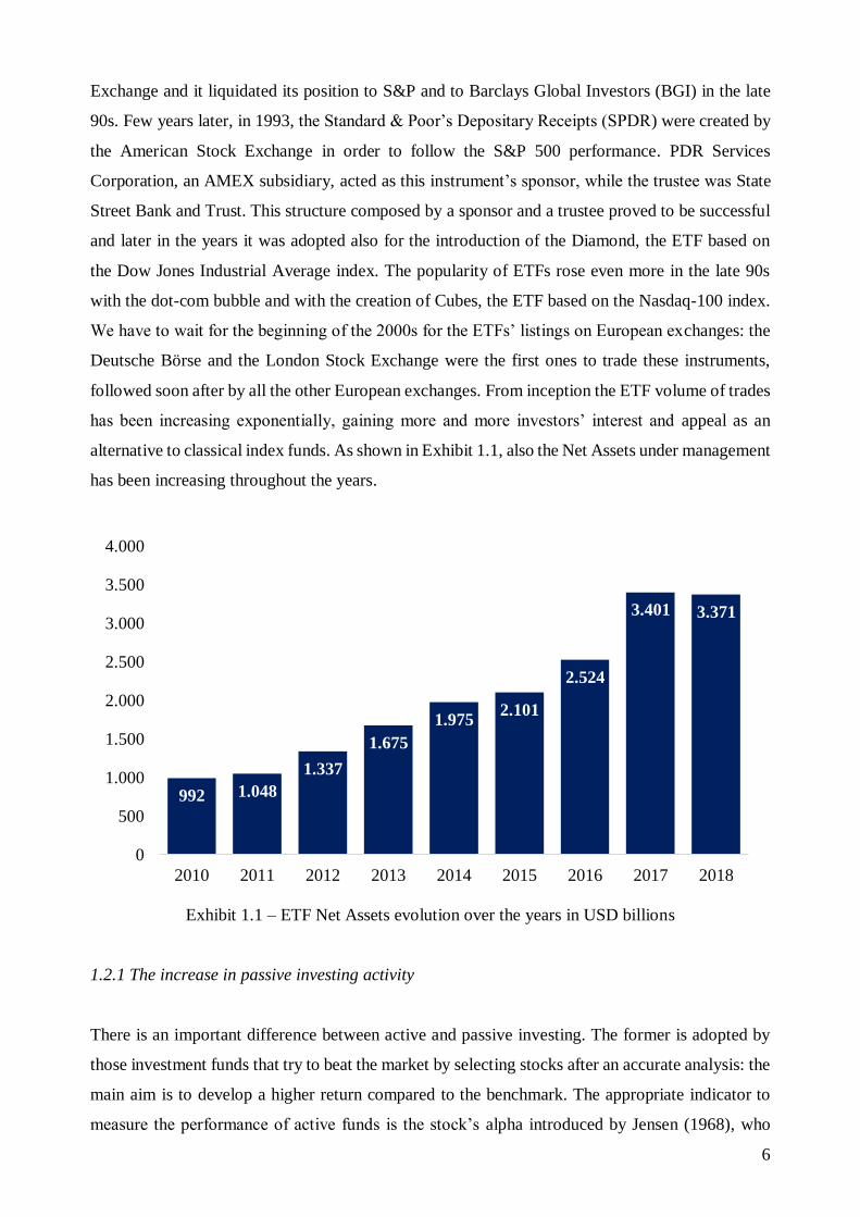
followed soon after by all the other European exchanges. From inception the ETF volume of trades

has been increasing exponentially, gaining more and more investors’ interest and appeal as an

alternative to classical index funds. As shown in Exhibit 1.1, also the Net Assets under management

has been increasing throughout the years.

Exhibit 1.1 – ETF Net Assets evolution over the years in USD billions

1.2.1 The increase in passive investing activity

There is an important difference between active and passive investing. The former is adopted by

those investment funds that try to beat the market by selecting stocks after an accurate analysis: the

main aim is to develop a higher return compared to the benchmark. The appropriate indicator to

measure the performance of active funds is the stock’s alpha introduced by Jensen (1968), who

992 1.048

1.337

1.675

1.9752.101

2.524

3.401 3.371

0

500

1.000

1.500

2.000

2.500

3.000

3.500

4.000

2010 2011 2012 2013 2014 2015 2016 2017 2018

7

defined this indicator as the average incremental rate of return on the portfolio which can be

explained by manager’s ability to forecast future security prices. It is important to point out that

this measure can be either positive (when the fund outperforms the benchmark and its expected

return) or negative (when the fund underperforms the benchmark and its expected return). The

latter instead is adopted by funds whose aim is not to overperform, but to generate the same return

of the benchmark. The tracking error is a more appropriate measure of their performance, since

investors are not interested in a premium return but in the same return of the index.

Index investing became more and more popular in recent years, with no distinctions in this trend

based on investors’ type: it is a phenomenon that concerns both individual and institutional

investors. One of the main reasons backing this decision by investors might be the high fees charged

by active funds compared to the ones of the passive ones: in fact, there is evidence that passive

investments produce a similar or even better return thanks to their cost efficiency. Exhibit 1.2 shows

the expense ratio in percentage of both actively and passively managed funds. Both of them

consistently decreased over the years, but passively managed funds still show a better efficiency

and lower costs compared to the active ones.

Exhibit 1.2 – Expense ratio of Actively managed and Passively managed funds

Furthermore, it seems that through passive investing arbitrage opportunities disappear and the

market becomes more efficient. According to Dellva (2001), indexing has been popular due to

three factors: lower cost, lower turnover and competitive performance results that are not so

dissimilar from the ones of actively managed funds. As explained by Anadu, Kruttli et al. (2018),

passive management has positive and negative effects also on financial stability. For example,

0,940,99 0,96

0,92 0,92 0,89 0,86 0,84 0,820,78 0,76

0,17 0,17 0,15 0,14 0,13 0,12 0,11 0,11 0,09 0,09 0,08

0

0,2

0,4

0,6

0,8

1

1,2

2008 2009 2010 2011 2012 2013 2014 2015 2016 2017 2018

Actively managed Passively managed

8

passive vehicles as ETFs reduce risk of liquidity transformation thanks to the redemption in kind

process: cash redemptions instead could lead to some fire sale by fund managers and destabilizing

redemptions. In contrast with this effect, it seems that some passive investment strategies, as those

using leverage exchange-traded products, increase market volatility. As explained by Ben-David

et al. (2017), ETFs can cause some liquidity shocks in the underlying securities and fluctuations in

demand that makes prices of those assets more volatile

1.3 What is an ETF?

An ETF is a marketable security that provides investors with an ownership right over an underlying

basket of assets, through a passive low-cost diversification strategy. Fund managers do not have

the possibility to design and to alter the fund’s composition at their discretion since the ETF’s

strategy is given in advance and one of its main features is the reduction of management fees.

They also offer the possibility to easily reach asset classes and markets that otherwise investors

could not have reached such as emerging markets and commodities. In fact, over the years we saw

the introduction of several exchange-traded products (ETPs) such as exchange-traded commodities

(ETCs) that track individual commodities or a basket of these with the advantage of not having to

bear storage costs and exchange-traded notes (ETNs), which are a type of unsecured debt security

designed to track market benchmarks.

Exchange-traded funds represent a claim against the assets held in the trust. Their main features

are their tax efficiency, low expense ratios and intraday trading.

Starting from the first one, investors can use ETFs in order to avoid huge tax expenses through the

in-kind redemption process, compared to mutual funds’ investors who have to bear capital gains

not only during distributions, but also when other shareholders leave the fund. When an investor

decides to sell its ETF, he sells the shares to other traders or market makers, with no need for the

fund to dismiss any stock in the underlying portfolio.

ETFs also have fewer chargeable expenses compared to the ones of mutual funds, which usually

charge their investors of fees as operating expenses (including administrative expenses and

advisory fees), front-end and back-end loads (paid when shares are purchased or sold) and 12b-1

charges (used to pay advertising costs and commissions for brokers). However, we are going to see

in the next chapters the impact of each fee, in order to determine the aggregate amount of the

expense ratio.

We can also distinguish physical and synthetic ETFs: the first ones hold the underlying assets in a

trust, with the advantage that there is more transparency concerning holdings and investors’ claim,

9

the second ones, instead, try to replicate the performance of the benchmark using swaps and other

derivatives, giving investors some other advantages as lower costs and lower tracking error.

1.3.1 The creation and redemption process

It has been of great interest the singularity of the creation and redemption process of the ETFs. In

fact, it represents at the same time an arbitrage opportunity, made possible by the misalignment

between ETF’s price and NAV, and a way to avoid taxes on capital gains. As we said before, by

delivering portfolio securities to shareholders in exchange of their ETF shares capital gains are

avoided and decisions about the portfolio are based only on investment considerations. ETFs are

structured as open-end funds so that there isn’t a fixed number of shares outstanding, but it can

vary over time according to transactions.

The creation process happens in the primary market, where a sponsor agrees with a large

institutional investor, called the Authorized Participant (AP), to buy a certain number of shares that

tracks some specific market index. The AP buys the shares and gives them to the sponsor, who

places them in a trust. The sponsor gives the AP a block of ETF shares, called the creation unit,

which are then traded on the exchange. The creation unit size may vary on funds’ discretion,

ranging from 25,000 to 300,000 shares. Each instrument represents a claim against the shares held

in the trust. It is important to notice that the AP cannot buy ETF shares using exclusively cash. As

explained by Deville (2008), in some situations the AP may be asked to deposit not only a portfolio

of securities, but also some additional balancing cash equal to the difference between the Net Asset

Value (NAV) and the share price that represents dividends cumulated by the fund, management

fees and adjustments due to rounding. Once the ETFs are created, institutional investors and other

market makers start to trade them on the secondary market.

Picture 1.1 – The creation process

Authorized ParticipantStock Market

Cash

Stocks

Deposits Creation Unit

(Securities + Cash)

Receives Fund SharesETF Trust

Broker / Dealer Individual Investor

Cash Stocks

Receive Fund Shares

Cash

10

The redemption process is symmetrical to the creation process, since investors willing to liquidate

their position can sell ETFs to market makers and institutional investors, who will collect again

ETF shares and redeem them in exchange of the underlying portfolio of securities held by the trust

plus a cash amount. The only requirement is to deliver ETF shares in creation units, as ETFs cannot

be redeemed in single units. As we will see, most of the ETF benefits stem from this

creation/redemption process.

Picture 1.2 – The redemption process

1.3.2 Tax efficiency of ETFs

In many countries, investment companies’ regulation is designed in order to give shareholders

some tax advantages: in fact, usually investors pay taxes just on funds’ distributions of dividends

and on capital gains. ETFs instead, due to their particular structure, receive a different tax treatment.

Associated with the redemption in kind process, the tax benefit that investors can exploit from this

financial instrument is given by ETF’s ability to minimize capital gains for taxable investors. This

mechanism avoids the creation of taxable income and unrealized gains inside an ETF. In the

redemption process, retail investors sell their fund shares to market makers and other institutional

investors, who then exchange them with the portfolio of securities locked into the fund. There is

also an advantage for the fund’s managers as in case of redemption they can turn their less taxable

creation units minimizing realized gains that must be delivered to shareholders and, then, taxed.

This benefit is more evident in ETFs that hold common stocks that often see capital gains compared

to bond funds. An example provided by Poterba and Shoven (2002) can be useful in order to explain

better the process: suppose that an institutional investor decides to redeem ETF shares with a

market price of $100,000 for $100,500 of underlying stock value. The capital gain for the

institutional investor here is $500. However, if the fund manager returns securities with a lower

Stocks

Authorized ParticipantStock Market

Cash

Deposits Fund Shares

Receives Underlying SharesETF Trust

Broker / Dealer Individual Investor

Cash

Cash

Sells Fund Shares

Stocks

(Lowest Cost Securities)

11

basis (i.e. the price that serves as a basis for capital gains calculation) than the ETF shares’ one,

capital gains are deleted for investors, who then are tax-exempt. This mechanism mainly impacts

market makers and institutional investors that trade in the primary market. However, as introduced

before, also for individual investors there are some implications. As opposed to mutual funds,

whose remaining shareholders have to bear taxes for realized and unrealized capital gains of the

ones that leave the fund, ETFs’ investors are taxed for their personal realized capital gains.

1.3.3 Intraday trading option

As we introduced before, it is possible to trade ETFs during the day. In this way investors are not

bound to the mutual funds’ policy to buy and sell shares at the end of the trading day. This intraday

trading option gives them the possibility to exploit some opportunities due to bid/ask spreads.

Furthermore, ETFs have two different prices: the NAV of the underlying assets and the market

price determined by trading on the exchange. We will see what this distinction of prices means and

what it will cause in the next paragraph. As we can see from Exhibit 1.3, the number of net

issuances in the U.S. has increased over the years: in the after-crisis years we can see a stable trend,

while in the following years there is a sharp increase, meaning that creation processes exceeded

redemption processes, showing how these instruments are becoming more and more appealing.

Exhibit 1.3 – Net Issuance of ETF shares in USD billions

Risk management issues as well can be addressed by traders using ETFs’ intraday feature as a

short-term solution. Another tool that stems from the intraday trading option possibility is the short

116 118 118

185 180

241 231

284

471

311

0

50

100

150

200

250

300

350

400

450

500

2009 2010 2011 2012 2013 2014 2015 2016 2017 2018

12

selling. ETFs are allowed to be short-sold on the market and this activity accounts for a significant

part of the trading volume. However, Gastineau (2001) shows that short selling can create several

risks: it is possible that the ETF portfolio changes between the date of the short-sale and the day of

the purchase, incentivizing portfolio managers to keep the same weight balance of each security in

the fund’s portfolio and limiting orders for some securities. However, cap-weighted index ETFs

are the most used instruments for short-sales, since it is very hard to suffer from a short squeeze

for the high liquidity of the stocks in the portfolio: these ETFs are usually short-sold in order to

cover the systematic risk of another long positions. Finally, we have leveraged ETFs that provide

long or short exposure to the daily return of various indexes, sectors and assets. Leveraged ETFs

attract investors since provide short-term strategies to hedgers and speculators, giving them the

possibility to bet on the market in an easy way. These securities are designed to return either

positive multiples (2x or 3x) or negative multiples (-2x or -3x) of the daily performance of the

underlying index. These amplified returns are achieved through total return swaps, other

derivatives and debt. There are some differences between ETFs and leveraged ETFs. As explained

by Li and Zhao (2014), there are three major differences:

• Leveraged ETFs must be rebalanced on a daily basis to generate promised returns. That is, the

notional amount of the total return swap has to be modified according to fluctuations of the

fund’s NAV;

• Leveraged ETFs are more expensive (in terms of expense ratio) than traditional ETFs;

• Leveraged ETFs do not dispose of the creation and redemption process in kind since they

typically use derivatives and do not actually hold any underlying security.

1.3.4 ETF’s price and Net Asset Value dynamics: the arbitrage opportunity

The Net Asset Value (NAV) represents the difference between assets and liabilities divided by the

number of shares. As with index funds, the NAV is computed at the end of each trading day (at 4

p.m.), and creation/redemption transactions occur at NAV. Since in ETFs shareholders just bear

the transaction cost of the purchase and sale, the NAV is designed in order to protect existing

shareholders from new investors’ trading costs. It is possible to buy ETF shares below NAV or to

sell them above it, according to the changes in supply and demand in the market. By the way, the

in-kind creation and redemption processes are able to adjust these deviations and to avoid

significant losses for shareholders. When the ETF price falls below the NAV, it could be profitable

for APs to short sell index stocks, buy ETFs and redeem them for the underlying portfolio,

generating in this way a profit. However, the efficiency in the pricing process of ETFs relies on

13

transaction costs and cash balances delivered to the trust: these mechanisms should prevent APs

from making a significant profit. Moreover, ETF prices are updated every 15 seconds, giving the

possibility to understand quickly how to trade in order to align prices with the NAV. Gastineau

(2001) also highlights that the market is too efficient to create a significant arbitrage opportunity

for such investors and that trading fees have to be considered as well. Market makers will

participate at both intraday trading and NAV-based trading in order to react to some liquidity shock

that might arise in the secondary market. They will post bids and offers according to the NAV

proxy and change them any time there are changes in retail investors’ orders, in liquidity of

underlying securities and in the cost of creating/redeeming ETF shares. Market makers’ aim is to

not expose themselves but to hold a balanced position: so, they need to monitor constantly the net

sales and purchases and respond holding a neutral position through the creation and redemption

processes. Another important feature of ETFs is their transparency: differently from mutual funds,

which report their holdings quarterly or with 60-days delay, ETFs provide daily information about

their holdings. Such information becomes critical for the arbitrage activity done by market makers

and APs: without this transparency it becomes harder to align the securities’ price with their NAV.

Therefore, the arbitrage opportunity for these market participants ensures that market price and

NAV is approximately equal. At the beginning of each trading day, the fund states the composition

of the underlying securities in its portfolio: during the day, market participants trade both ETF

shares and the underlying assets, eventually causing misalignments. As an example, suppose the

NAV is $100.00 and ETF price goes down to $99.50: APs could then buy shares for $99.50 and

exchange them for underlying securities worth $100.00. This process drives the ETF price up,

reducing the difference in prices and producing a profit of $0.50 for the APs. Now suppose that the

ETF price goes up to $100.50: similarly, the APs could sell shares on the market for $100.50 and

create new ones at a NAV of $100.00, resulting in a profit of $0.50 as well.

1.4 Mutual funds and Index funds

Over the years index investing has become a popular investment vehicle in fund management.

According to Meade and Salkin (1990), institutional investors such as pension funds and insurance

funds dominate the stock market, and their managers are very often bound to this policy of index

tracking, in order to diversify away specific risk and hold just the undiversifiable market risk.

Equity index funds can be divided into open-end, where cash flows in and out according to the

needs of the investors, and closed-end, where a fixed amount of money is invested for an

indeterminate period.

14

A mutual fund is an investment company that gathers money from individuals and uses those funds

to trade securities. Portfolio management here deals both with asset allocation and security

selection decisions. Investors who buy shares of the fund delegate the investment decision to

professional fund managers. The one thing that really distinguish mutual fund investing is that it

attracts both experienced and inexperienced individuals with different income levels and different

purposes: the inexperienced ones can use them since they might not have the same information as

fund managers, while the experienced ones can use them in order to protect themselves or to

diversify. In the following Exhibit 1.4 we can see how Net Assets under management of index

equity mutual funds has increased over the years, which is in line with the passive investing rise.

Exhibit 1.4 – Total Net Assets of Index Equity Mutual Funds in USD billions

Mutual fund’s price moves accordingly with the price movements of the securities it holds and

when the fund receives interests and dividends, these are then either distributed to the fund’s

shareholders or reinvested by purchasing more shares in the fund.

The organisation of mutual funds can be complex since all the fund’s tasks as investing, record

keeping and brokerage are divided between different companies. We have the fund itself, usually

organized as trusts, which is owned by its shareholders. A management company is responsible for

all the daily operations of the fund and acts as investment advisor. An investment advisor trades

securities and supervises the fund’s portfolio, it includes: a money manager, accountable for buying

and selling decisions, a securities analyst and traders. Then there is a distributor who is responsible

for selling shares both on the primary and secondary market, a custodian, usually represented by a

bank whose role is to oversee fund’s securities and other assets, and a transfer agent, who records

678824 856

1.031

1.429

1.6801.789

2.133

2.7402.654

0

500

1.000

1.500

2.000

2.500

3.000

2009 2010 2011 2012 2013 2014 2015 2016 2017 2018

15

the shareholders’ request to create and redeem new shares. This complex segregation of duties has

the specific aim to avoid conflict of interests and to protect retail investors: in the structure

described previously, the management company does not hold the fund’s asset, so it is hard to take

advantage and exploit other opportunities that do not accomplish the shareholder’s investment

objectives.

1.4.1 Index funds characteristics

As we already said previously, index funds try to perform as a broad market index. The fund also

buys and sells shares according to the proportion of each share in the index. As an example,

Vanguard 500 Index Fund tracks the S&P500 index: since this index is value-weighted, the fund

buys securities in proportion to the market value of that company’s outstanding equity.

As explained by Bogle (2016), index fund’s operations are not complex at all: fund’s managers

have to buy and hold stocks that compose the benchmark index and lower any kind of cost from

advisory fees and operating costs to portfolio turnover. These investing instruments allow small

investors to pursue a passive investment strategy at a reasonable price and effortlessly.

According to Gitman et al. (2010) the main reasons for investing in mutual funds are three:

• Accumulation of wealth. Investors’ aim is to build capital over the long run, carrying a

moderate amount of risk.

• Storehouse of value. Investors consider mutual funds a “safe” place where to store money,

without exposing the initial capital to huge losses. For this purpose, short- and intermediate-

term bond funds are a reasonable option.

• Speculation and short-term trading. Some investors consider mutual funds to be attractive for

speculation: traders can buy and sell shares of the fund according to the investors’ sentiment

Other than equity index funds, we can see also bond index funds and real estate index funds, which

can attract investors with specific needs. Assets under management of index funds have risen

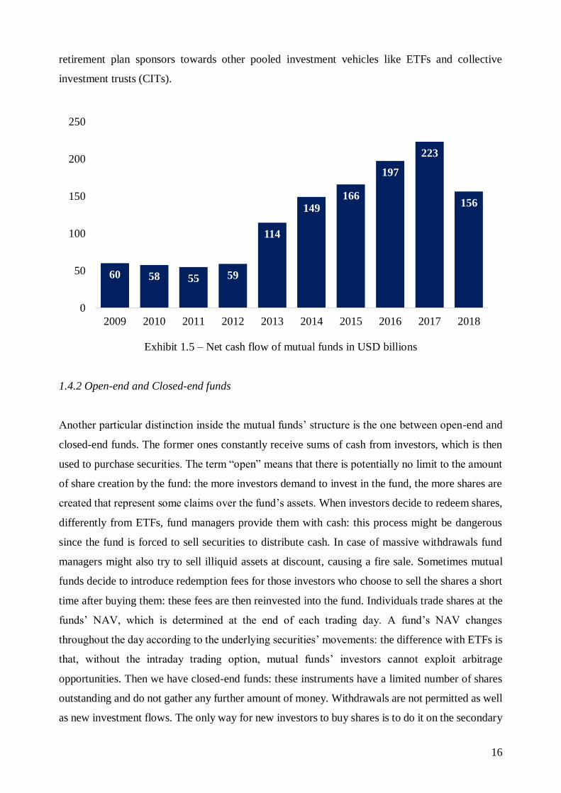
sharply over the years. As shown in Exhibit 1.5 cash flows as well, which reflect investor’s demand

for mutual funds and is calculated as cash inflows minus cash outflows, have increased over the

years. In the after-crisis years we can see how investors’ sentiment has driven performance, with

low amounts of net cash inflows, while in the following years this number grew strongly, according

to the bull market cycle of these years. The reduction of cash flows during 2018, according to the

Investment Company Institute Factbook 2019, was mainly due to the shift of investors and

16

retirement plan sponsors towards other pooled investment vehicles like ETFs and collective

investment trusts (CITs).

Exhibit 1.5 – Net cash flow of mutual funds in USD billions

1.4.2 Open-end and Closed-end funds

Another particular distinction inside the mutual funds’ structure is the one between open-end and

closed-end funds. The former ones constantly receive sums of cash from investors, which is then

used to purchase securities. The term “open” means that there is potentially no limit to the amount

of share creation by the fund: the more investors demand to invest in the fund, the more shares are

created that represent some claims over the fund’s assets. When investors decide to redeem shares,

differently from ETFs, fund managers provide them with cash: this process might be dangerous

since the fund is forced to sell securities to distribute cash. In case of massive withdrawals fund

managers might also try to sell illiquid assets at discount, causing a fire sale. Sometimes mutual

funds decide to introduce redemption fees for those investors who choose to sell the shares a short

time after buying them: these fees are then reinvested into the fund. Individuals trade shares at the

funds’ NAV, which is determined at the end of each trading day. A fund’s NAV changes

throughout the day according to the underlying securities’ movements: the difference with ETFs is

that, without the intraday trading option, mutual funds’ investors cannot exploit arbitrage

opportunities. Then we have closed-end funds: these instruments have a limited number of shares

outstanding and do not gather any further amount of money. Withdrawals are not permitted as well

as new investment flows. The only way for new investors to buy shares is to do it on the secondary

60 58 55 59

114

149166

197

223

156

0

50

100

150

200

250

2009 2010 2011 2012 2013 2014 2015 2016 2017 2018

17

market: the trading is made between retail investors themselves and they do not engage with the

funds’ managers. Consequently, it is possible to buy closed-end fund’s shares only during the

trading day: the market price can then deviate from the NAV (as with ETFs), causing the fund to

trade at a premium or at a discount. Gitman et al. (2010) show that usually closed-end funds trade

at a discount for several reasons:

• They usually hold more illiquid assets than open-end funds, so that in case of a fire sale huge

value gets lost;

• Shares held by the fund might be subject to taxation (i.e. unrealized capital gains) and investors

would bear those costs;

• Investor sentiment can drive prices away from fund’s NAV

Since closed-end funds trade like stocks, brokerage fees are applied to investors. Open-end funds

instead are bought and sold from the fund operators, without dealing with any broker. Liquidity

also differs because it is possible to trade open-end funds at any time at its NAV, while we have

seen that closed-end funds might create some liquidity problems to both investors and fund

managers.

1.4.3 Mutual funds expense ratio

Both closed-end and open-end funds apply commissions and management fees to their

shareholders. The most common ones are operating expenses, front-end loads, back-end loads and

12b-1 charges. Operating expenses are those administrative costs, marketing costs and advisory

fees paid to the investment managers who run the fund’s operations. They usually range between

0.2% and 2% of the total assets under management and they are used also to pay brokers who sell

shares to the public. Front-end and back-end loads are commissions paid when investors buy or

sell the fund’s shares and they are used to pay brokers or to retain investors’ money into the fund

for a longer period of time. There are also no-load funds that do not apply these fees and do not

reduce the amount of money invested by individuals. Finally, it is possible to include 12b-1

charges, which represent distribution costs, advertising costs and provisions of annual reports and

prospectuses. Different mutual funds structure their fees according to the investment policy and to

shareholders’ interests. As an example, index funds result one of the cheapest form of funds since

the aim of replicating the performance of a benchmark does not require any kind of research effort

or advice from professionals. However, as explained by Bodie et al. (2014), some investors are

18

willing to bear these costs since they can dispose of advisors and managers who provide them of

their financial aid.

The several expenses that are charged to investors reduce the overall performance and rate of

return, because such expenses are usually deducted from the fund’s net asset value. Furthermore,

investors have to pay such expense regardless of the good or bad return earned by the fund.

Obviously, expense ratios are higher for actively managed funds since operations require more

efforts and fund managers ask for a higher compensation in order to beat the market and to gather

information about specific market sectors and geographic regions. Total net assets of passive index

funds are concentrated on large-cap stocks such as the ones included in the S&P500, while the total

net assets of actively managed funds are more dispersed and include mid- and small-cap stocks that

result to be more expensive to manage.

1.5 A comparison between Index Funds and ETFs

After having exposed the characteristics of both ETFs and index funds, we are able to make a

comparison between the two securities. What they have in common is the purpose to reproduce the

performance of some index benchmark, trying to lower costs and to hold the same stocks included

in the benchmark. They are both passive investing instruments and none of them aims to

overperform the market and they both try to reduce their tracking error. ETFs are similar to closed-

end funds since they trade on the stock market during the trading day and have a market price and

a NAV which can diverge. However, they are similar to open-end funds as they do not have a

limited number of shares outstanding and there is no limit when issuing shares for new

shareholders.

There is also a significant difference in the tax-treatment of these instruments, in particular for what

concerns capital gains. As we already said, the most particular process of ETFs is the

creation/redemption in kind process. According to Gastineau (2001), in mutual funds the absence

of this process causes portfolio managers to face a conflict of interest since they could either sell

the shares and distribute taxable capital gains or hold overvalued securities and miss capital gains.

Mutual funds do not pay taxes themselves but are required to distribute dividends and capital gains

on all shares outstanding. Index funds have a lower taxation discipline but still are required to

distribute capital gains to shareholders. We have already seen how ETF investors, thanks to the

creation/redemption process, receive benefits from a taxation perspective. In addition, ETF

shareholders pay the cost of creation and redemption (which is the cost of increasing and shrinking

the fund’s size), while for mutual funds traders can buy and sell shares at their net asset value,

19

causing all the other pre-existing shareholders to bear the costs for the creation and redemption

processes in terms of commissions.

Talking about costs, ETF shareholders bear just the transaction costs associated with the stocks

trading, mutual funds instead, in order to favour a no-commission entry for new investors, associate

to each existing shareholder a proportion of the costs. ETFs also offer lower operating expenses

than conventional mutual funds. One of the main disadvantage of ETFs, as we saw before, is the

bid/ask spread that can cause investors to pay more than the actual value of the security and can

highlight some arbitrage opportunities.

We have seen some of the costs that ETFs and index funds investors have to bear. The most relevant

cost of ETFs is the commission cost that is charged when investors buy or sell shares from

brokerage firms. For index funds instead, the main costs are associated with front-end loads, back-

end loads and 12b-1 fees. By the way, apart from these visible costs, there are some “invisible

trading costs” (Edelen, Evans and Kadlec, 2013, pp. 16) that individuals are not always aware of

when investing and that can significantly alter performance.

20

CHAPTER 2 – MAIN DRIVERS OF ETF FLOWS AND THE RETURN

CHASING BEHAVIOUR


This chapter represents a preliminary explanation of the variables employed in my model: thus, it

was my intention to include this section in order to illustrate the meaning and the purpose of these

variables and of this work.

In this chapter, a primary definition and calculation of ETF flow is provided, showing how such

measure is a representation of investor demand in the primary and secondary market.

Then, it is illustrated how the stock market activity represent an important factor for ETF flows,

including among the variables some measures of liquidity and the NAV Premium.

The central part of my work is the return chasing behaviour of ETF investors and a specific section

is dedicated to this topic, explaining the phenomenon and the difference with trend following.

After that, a paragraph is dedicated to the control variables included in the model, such as size and

age of the selected instruments, which are specific of each ETF, and market indexes and interest

rate, which reflect market trends and economic cycles.

Finally, it is possible to find an outlook of the European ETF market and its differences from the

American one, with the former representing still a growing and not mature market where retail

investors still do not hold a significant share of the market and the latter composed by a more

balanced mix of retail and institutional investors.

2.2 ETF Flows: definition and computation

Since ETFs have been one of the most successful funds of the last decades, it is interesting to focus

on the reasons and on the different uses of these financial instruments. As shown before, ETFs’

assets under management have been increasing constantly as well as investors’ demand for them.

In this framework and for the purpose of this work, the definition of ETF flow is provided.

ETF flow is essentially the investors’ demand for ETF shares and, since such money is invested by

funds’ managers, represents the growth in the fund’s assets under management.

As explained by Clifford et al. (2014), there are many market variables that can influence cash

flows into ETFs, varying from order imbalances, arbitrage opportunities and excessive spreads.

There are two different formulas that can be applied for ETF flows, following previous literature.

21

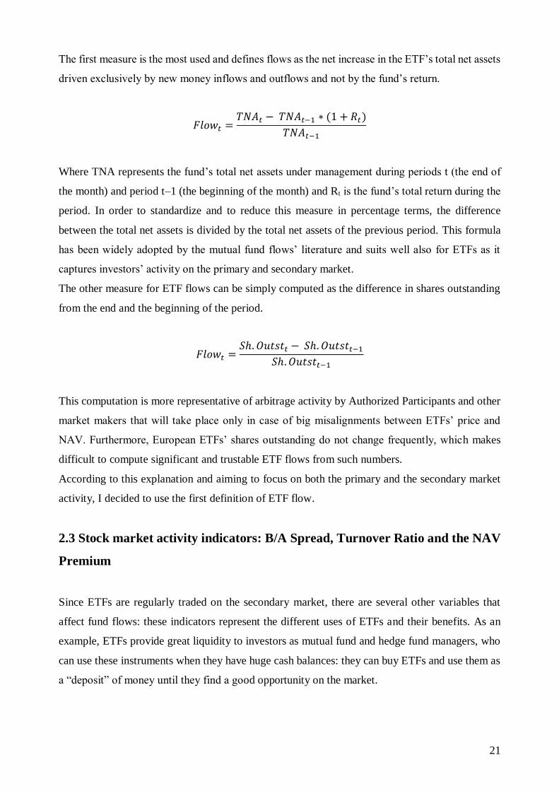
The first measure is the most used and defines flows as the net increase in the ETF’s total net assets

driven exclusively by new money inflows and outflows and not by the fund’s return.

𝐹𝑙𝑜𝑤𝑡 =𝑇𝑁𝐴𝑡 − 𝑇𝑁𝐴𝑡−1 ∗ (1 + 𝑅𝑡)

𝑇𝑁𝐴𝑡−1

Where TNA represents the fund’s total net assets under management during periods t (the end of

the month) and period t–1 (the beginning of the month) and Rt is the fund’s total return during the

period. In order to standardize and to reduce this measure in percentage terms, the difference

between the total net assets is divided by the total net assets of the previous period. This formula

has been widely adopted by the mutual fund flows’ literature and suits well also for ETFs as it

captures investors’ activity on the primary and secondary market.

The other measure for ETF flows can be simply computed as the difference in shares outstanding

from the end and the beginning of the period.

𝐹𝑙𝑜𝑤𝑡 =𝑆ℎ. 𝑂𝑢𝑡𝑠𝑡𝑡 − 𝑆ℎ. 𝑂𝑢𝑡𝑠𝑡𝑡−1

𝑆ℎ. 𝑂𝑢𝑡𝑠𝑡𝑡−1

This computation is more representative of arbitrage activity by Authorized Participants and other

market makers that will take place only in case of big misalignments between ETFs’ price and

NAV. Furthermore, European ETFs’ shares outstanding do not change frequently, which makes

difficult to compute significant and trustable ETF flows from such numbers.

According to this explanation and aiming to focus on both the primary and the secondary market

activity, I decided to use the first definition of ETF flow.

2.3 Stock market activity indicators: B/A Spread, Turnover Ratio and the NAV

Premium

Since ETFs are regularly traded on the secondary market, there are several other variables that

affect fund flows: these indicators represent the different uses of ETFs and their benefits. As an

example, ETFs provide great liquidity to investors as mutual fund and hedge fund managers, who

can use these instruments when they have huge cash balances: they can buy ETFs and use them as

a “deposit” of money until they find a good opportunity on the market.

22

2.3.1 ETFs’ liquidity: Bid-Ask Spread and Turnover Ratio

Liquidity represents one of the most important features in the stock market and one of the most

relevant aspects to consider when trading. We can think of liquidity as the availability of cash in

relation to the demand of assets on the market, or as the ability of stock markets to absorb

fluctuations in demand and supply without any change in securities’ prices. An asset is said to be

liquid when it is easily convertible in cash without incurring in a substantial loss in value or in

significant transaction costs. Sarr and Lybek (2002) state that liquidity measures can differ

according to market sentiment: in fact, during stable periods it can be reflected by trading costs,

while during more turbulent periods prompt price discovery and adjustments to new equilibrium

are more valued. In opposition to this, illiquidity can be seen in those markets where daily prices

are affected by large fluctuations (higher volatility) and where daily transactions are low as well.

These characteristics allow investors to chase higher returns (in particular the higher volatility),

even if some of them may be locked in their position because of high trading costs, high bid-ask

spread and unavailability of a counterparty willing to trade.

ETFs’ specific tool of creation and redemption provides an extra liquidity to investors: according

to Abner (2016), the possibility to continuously increase and decrease the number of shares

outstanding in order to accomplish market demand avoids some illiquidity problems that can arise

from the unavailability of tradable shares. Abner (2016) also explains that liquidity providers,

defined as market makers who act aiming to satisfy their clients’ order flows, can use the

creation/redemption mechanism to exchange underlying assets with ETFs and vice versa, offsetting

their positions and providing constant liquidity in the market.

In this framework, one of the main indicators of market liquidity is the Bid-Ask Spread, which is

defined by the market makers as a remuneration for their services and for the costs of holding

inventory. This measure is considered the most relevant transaction cost: when the spread is huge,

traders tend to leave the market or to focus on other asset classes, shrinking the breadth (the

capacity to have minimal impact on prices even with large and numerous orders) and the resiliency

(the presence of new orders and inflows that correct previous imbalances) of the market. It can be

computed as the difference between the bid and ask quotes, or as the difference of the bid and ask

quotes taken as a percentage of the mid price.

𝑆 = (𝑃𝐴 − 𝑃𝐵)

𝑆 =(𝑃𝐴 − 𝑃𝐵)

(𝑃𝐴 − 𝑃𝐵

2 )

23

Other than transaction cost measures, there are some volume-based indicators used to assess the

depth (the existence of abundant orders) of the market. The most traditionally used measure for

liquidity is the trading volume, which is also an indicator of the number of market participants and

transactions. The number of trades is a fundamental information since it allows dealers and brokers

to properly allocate order flows, understanding which quoted prices are effective and fixing

imbalances between buyers and sellers. Therefore, the average daily volume (ADV) represents the

number of shares traded over a certain period of time. It is given by:

𝐴𝐷𝑉 = 𝑆𝑢𝑚 𝑜𝑓 𝑡ℎ𝑒 𝐷𝑎𝑖𝑙𝑦 𝑉𝑜𝑙𝑢𝑚𝑒

# 𝐷𝑎𝑦𝑠 𝑜𝑓 𝑇𝑟𝑎𝑑𝑖𝑛𝑔

Usually, the 30 days average volume is a good proxy for a stock’s liquidity. The higher the ADV,

the higher the liquidity of the stock traded. In addition to this, investors compare the ADV to the

size of their order since through a large trade they can impact stock prices.

The turnover rate is another measure widely used to assess market liquidity. It is computed as:

𝑇𝑛 =𝑉𝑜𝑙𝑢𝑚𝑒 𝑜𝑓 𝑇𝑟𝑎𝑑𝑒𝑠

(𝑆ℎ𝑎𝑟𝑒𝑠 𝑂𝑢𝑡𝑠𝑡𝑎𝑛𝑑𝑖𝑛𝑔 ∗ 𝐴𝑣𝑒𝑟𝑎𝑔𝑒 𝑃𝑟𝑖𝑐𝑒 𝑜𝑓 𝑆ℎ𝑎𝑟𝑒𝑠)

This ratio shows the percentage of a fund’s holdings that have changed during the year and is a

good estimate of its trading activity. The turnover rate is useful in order to distinguish actively and

passively managed funds, with the former showing higher ratios and the latter showing lower ones.

According to Broman and Shum (2018) ETFs also help investors to avoid massive transaction costs

that they could have suffered from trading the underlying basket. ETF liquidity favours short term

ownership and trading, creating a liquidity clientele. In fact, institutional investors use ETFs for

different purposes as tactical asset allocation, cash equitization and liquidity management.

ETF liquidity for this reason should predict fund flows as it facilitates trading in terms of aggregate

demand.

2.3.2 The NAV Premium

As explained in chapter 1, ETFs are characterized by both prices on the market and net asset value

(NAV) representing underlying assets. During trading days, it is possible to see differences

between these two values according to the market activity. Engle and Sarkar (2006) state that

underlying shares delivered at the end of the day does not help in adjusting intraday distortions and

24

create more uncertainty and volatility across the market. In addition to this, long delivery periods

and price risks make the arbitrage mechanism more complex and costly.

Authorized Participants act in order to delete these discrepancies, finding some remuneration from

the arbitrage opportunity, as they can trade in the primary or in the secondary market whenever it

is more convenient. For this reason, ETF flows should be positively influenced by existing

premiums. According to Broman and Shum (2018), as the activity by APs occurs at daily or

intradaily interval, premiums only persist for few days. Following their methodology, the NAV

premium has been calculated as the average of the daily premiums over the entire month, where

the premium has been computed as:

𝑃𝑅𝐸𝑀𝑡 = ln(𝐿𝑎𝑠𝑡 𝑃𝑟𝑖𝑐𝑒𝑡) − ln(𝑁𝐴𝑉𝑡)

Where the last price and the NAV are daily observations and monthly premiums are then computed

as average of all the daily premium observations. The authors state that following this procedure it

is possible to highlight the excess demand that has not been arbitraged yet by market makers.

In addition, Clifford et al. (2014, pp. 627) state that the activity by AP “can potentially lead or lag

true investor flow” by front-running shares or waiting and responding slowly to investor demand:

however, this effect is shrunk by the adoption of monthly data as it is rarely present on a frequency

longer than few days.

2.3.3 The IDTS measure and its meaning

In addition to the variables already presented for market liquidity, the Bloomberg Terminal

proposes an alternative measure based on the underlying assets’ ADV and their percentage

contribution to the creation unit. As we can see in the Bloomberg page about liquidity of ETFs (i.e.

<LQA> function), in the trading data box the data about ADV and implied liquidity differ widely.

The implied liquidity indicator is based on the Implied Daily Tradable Shares (IDTS) measure of

the underlying securities. This number is showing how many ETF shares can be issued considering

the availability of its components. The IDTS formula is given by:

𝐼𝐷𝑇𝑆 =30 𝐷𝑎𝑦𝑠 𝐴𝐷𝑉 ∗ 𝑉𝑃

𝐶𝑜𝑛𝑠𝑡𝑖𝑡𝑢𝑒𝑛𝑡 𝑆ℎ𝑎𝑟𝑒𝑠 𝑝𝑒𝑟 𝐶𝑟𝑒𝑎𝑡𝑖𝑜𝑛 𝑈𝑛𝑖𝑡∗ 𝐶𝑟𝑒𝑎𝑡𝑖𝑜𝑛 𝑈𝑛𝑖𝑡 𝑆𝑖𝑧𝑒

Where 30 Days ADV is the ADV over the previous 30 days, VP is a variable percentage defaulted

to 25% and the Constituent Shares per Creation Unit looks at the number of shares required in the

25

portfolio. This data is computed for each security in the basket and the smallest IDTS becomes the

appropriate indicator for ETFs’ liquidity, since it represents a restriction on how many shares can

be issued. As reported by Abner (2016), the ETF volume embodies a historical number showing

past trades. The ETF implied liquidity instead is a forward-looking measure displaying how many

ETFs can be traded in the future coherently with the liquidity of underlying stocks.

However, since it is hard to gather historical data on this measure, this variable has been omitted

from the model.

2.4 ETFs’ performance and the return chasing behaviour of investors

In the academic literature there are some studies that highlight the naïve behaviour of some

investors consisting of putting money on those stocks and funds that performed well during

previous periods. This attitude is documented despite the fact that there is no evidence of the

predictive power of past performance over future returns.

Following these premises, it appears that the return chasing behaviour is simply a form of

extrapolation bias where market participants overweight recent events in their decision-making

process.

As explained by Haghani and McBride, it is possible to spot a difference between trend followers

and return chasers, where the former “proactively follow a pre-defined set of rules, which are well

documented in the academic literature” and the latter “act in a more discretionary and reactive way”

and are “unaware of their behaviour, creating a slower moving, self-reinforcing herding

phenomenon, based on the simple, readily available and intuitively appealing heuristic of recent

past returns” (2016, pp. 3). Also, they highlight how differences in returns gained by return chasers

and returns of funds they invested in are mainly due to the poor market timing ability of investors

and the poor dynamic selection of funds (not providing money to the best funds available but on

inferior ones).

Chien (2014) shows how expectations and experience are fundamental aspects in the stock market

and are valuable to investors: expectations about future market returns are strictly linked with past

market returns, even though rarely they meet actual future returns. The author also state that these

expectations affect portfolio decisions made by market participants and that “return chasing

behaviour may be costly for mutual fund investors. Given that stock market returns are essentially

unpredictable in the short run and move back to the average in the long run, return chasing

behaviour can miss the market timing – that is, investors may buy when prices are too high and sell

when prices are too low” (2014, pp.1).

26

Other working papers focused on the return chasing conduct with similar conclusions: Elton et al.

(2004) reported that investors value fund returns comparing them to the performance of indexes or

other funds and that should be concerned about the capacity of such funds of replicating the index

and about their risk; Ippolito (1992) explains that fund investors assess the quality of mutual funds

by examining recent risk-adjusted performance and Sirri and Tufano (1998) affirm that return

chasers put money into funds with high recent returns but fail to move out their holdings from poor

performers.

Comparing return chasing between ETFs and mutual funds, it is possible to spot some differences

in what drives the behaviour of investors. In the mutual funds industry, return chasing can be

explained by the willingness to allocate money to funds whose managers exhibit superior talent in

outperforming the market, even if such skill has been rarely documented (Berk and Green, 2004).

Furthermore, Chevalier and Ellison (1997) theorize a conflict between fund managers, who try to

maximize their value to raise their flow of investments but increasing also the riskiness of the fund

and investors who put money into the fund aiming to maximize their risk-adjusted return.

Fortunately, such issues are not applicable to the ETF environment, since ETFs are passively

managed funds and there is no concern about managers’ skills or personal ambitions.

For the analysis performed in this thesis, it was necessary to select the appropriate performance

measure in order to reflect the return chasing behaviour properly. Previous literature suggested for

two different measures: raw returns and risk-adjusted returns. Raw returns reflect the total return

accomplished by the fund during the period, combining price appreciation and reinvested

dividends. On the other hand, risk-adjusted returns are performance indicators that consider also

the risk born by the investor to produce the return: some of these measures include the Sharpe ratio

(that calculates the return in excess of the risk-free rate and divides it by the standard deviation the

those returns), the Treynor ratio (that calculates the return in excess of the risk-free rate and divides

it by the beta of the security) and Jensen’s alpha (that calculates the excess return of the security

over the expected return calculated according to the CAPM).

Mutual fund and ETF studies used both these measures, by the way, risk-adjusted measures appear

to be more adequate to mutual funds since these indicators may reflect fund managers’ ability to

process information: for this reason, raw returns seem more appropriate for simple return chasers

that base their choices on previous performance. Still, another issue is detected when talking about

the right time horizon that investors look at when they chase performance. Some investors can

allocate their holdings looking at previous returns on different time frames: in this analysis the

return chasing behaviour of investors is based on the average of the monthly total returns over the

previous year.

27

2.5 Control variables considered in the model

In the model designed for this analysis, it is necessary to include, other than market activity

indicators (that account for a liquidity clientele and for the arbitrage activity of Authorized

Participants) and fund total returns (that account for the return chasing investors), some variables

that capture other potential drivers of ETF flows, which can represent some ETF-specific

characteristics that investors implicitly consider and some global or macroeconomic factor that

drive investors away from the stock market.

2.5.1 Fund’s Size and Age

Two of the main control variables for the performance-flow relationship are funds’ size and age.

Intuitively, fund’s age and size are positively correlated, but their effects on fund flows might

differ.

If we consider size, it is easy to tell that funds need to reach a certain amount of assets under

management to accomplish desired returns. Furthermore, according to Indro et al. (1999) fund’s

size, expressed in terms of natural logarithm of total assets under management, is a measure of the

implicit transaction costs associated with the activities of fund managers. These transaction costs

“include the market impact of large fund’s trades on price and of the bid-ask spread, the opportunity

costs of not implementing trades, […] and deviations from style that result from a fund’s excessive

size”(1999, pp. 77). This last effect is not valid for ETFs since they are passively managed and

fund managers are not allowed to change their investing strategy.

Large funds should receive on average higher flows since they represent more established vehicles

compared to new and small funds, which still have not reached the dimension required to apply

successfully their replication strategies.

Age as well is another important variable for fund flows. Reasonably, new and young funds attract

more flows relative to their assets under management than old and established funds. Therefore, it

is possible to assume a negative relation between age and fund flows.

Both of these measures are expressed in natural logarithms:

𝑆𝐼𝑍𝐸 = 𝐿𝑁(𝑇𝑁𝐴 𝑎𝑠 𝑒𝑛𝑑 𝑜𝑓 𝑚𝑜𝑛𝑡ℎ)

𝐴𝐺𝐸 = 𝐿𝑁(𝐴𝑔𝑒 𝑒𝑥𝑝𝑟𝑒𝑠𝑠𝑒𝑑 𝑖𝑛 𝑛𝑢𝑚𝑏𝑒𝑟 𝑜𝑓 𝑦𝑒𝑎𝑟𝑠𝑓𝑟𝑜𝑚 𝑖𝑛𝑐𝑒𝑝𝑡𝑖𝑜𝑛)

28

2.5.2 Lagged fund flow and standard deviation of the daily volume

The other variables of the model include the lagged flow, expressed as the fund flow of the previous

month, and the standard deviation of the daily volume. The first one has been included in order to

account for some herd behaviour: the tendency to put money where other market participants

invested before.

I decided to include also the standard deviation of the daily volume as another variable to account

for liquidity in order to represent a variable for the lackness of liquity and the negative effect that

such variable has on fund flows. Such measure is simply calculated as the standard deviation of all

the daily volumes registered during one month. In addition, a volatile number for the daily volume

of trades alters the necessity of market makers and liquidity providers: in case of a highly variable

measure of liquidity, the work of these actors involves unexpected transactions and can lead to a

great effort in satisfying clients’ order flows.

2.5.3 Equity and Fixed Income Market indexes and the interest rate

Market trends and economic cycles are always important indicators when it comes to the evaluation

of investment decisions, since they give an overall picture of the market sentiment and of the global

performance of several industries and countries. Thus, some macro-indicators as market indexes

and interest rates can catch and explain some other relations that are not described from the

regressors included in this work.

Considering the European framework, there are several market indexes which provide a picture of

the European economy. The two most used European equity benchmarks are the EURO STOXX

50 and the STOXX Europe 600: the first one includes the stocks of the 50 biggest (in terms of

market capitalization) firms from 11 countries of the Eurozone, while the second one is composed

by 600 companies based in 17 countries of the European Union.

My decision to choose the monthly returns of the STOXX Europe 600 was based on the different

scope of this index, which includes large, mid and small capitalized companies, giving a

comprehensive portrait of the European market.

Additionally, the fixed income market plays a crucial role as well in detecting the investor

sentiment about the status of the economy. In this case the benchmark selected is the Bloomberg

Barclays EuroAgg Treasury 10+ Year TR Index (LET0TREU), an indicator of the European

government bond market whose fixed income holding have a maturity of over 10 years.

The returns of the Equity and Fixed Income indexes should have opposite effects on the European

ETF flows: when the equity market is performing well, investors are confident and put their money

29

on risky assets as stocks or ETFs that replicate some equity indexes, while during a recession or a

market slowdown they prefer safe instruments as government bonds. Therefore, I expect a positive

influence of the STOXX Europe 600 returns on ETF flows and a negative one of the LET0TREU

returns on them.

Finally, I decided to include the LIBOR rate since investors do not hold only equity investments

but they balance their portfolios according to the yield curve. Also, as explained by Santini and

Aber (1998, pp. 423), “higher interest rates decrease firm earnings and increase the cost of capital,

leading to the elimination of previously acceptable projects [Ibbotson et al. (1985)]”. In order to

report a variable about future expectations of the market, I used the 12-month LIBOR as a

benchmark for institutional investors, who should increase their holdings in equity ETFs when the

LIBOR rate decreases, implying a negative relation between these two variables.

In conclusion, my analysis is integrated by these three variables about macro-trends and indicators

representing the different needs of several investors (from retail to institutional).

2.6 The ETF market in Europe: trends and main providers

In this section I am going to illustrate the situation of the ETF market in Europe during the last

year, highlighting also some differences from the US market.

The European ETF market, as of June 2019, is composed by more products (2,812) compared to

the U.S. (2,291), despite the latter manage significantly more assets (3.9 trillion USD versus 878

billion USD). The high number of European products is a direct consequence of:

• The great market fragmentation;

• The huge presence of institutional investors and the limited participation of retail accounts

(about 15%);

• The possibility to offer ETFs in different share classes and currencies.

Another European peculiarity is the commission-based structure of the distribution channel

managed by banks. The adoption of a fee-based structure, in addition to the introduction of the new

regulation MiFID II that demands more cost transparency, could favour retail investors in the

evaluation of the true liquidity of these instruments.

During 2018, ETF flows halved compared to 2017 (43.5 billion EUR vs 97.9 billion EUR), with

flows converging towards defensive sectors such as healthcare and leaving highly volatile

industries. Still, this trend continued during the first months of 2019, with investors putting money

into fixed-income ETFs (14.3 billion EUR during Q1).

30

Another difference from the U.S. framework is the number of ETF providers: the European market

is divided among only few providers (i.e. BlackRock iShares, Amundi, UBS, Xtrackers, Lyxor)

and some important players in the U.S. market as Vanguard and Fidelity hold just a small share.

Exhibit 2.1 - Leading Providers of ETFs in Europe in 2017 by AUM

Finally, European ETFs charge higher fees with respect to U.S. instruments: for this reason, ETF

providers are constantly trying to lower their fees hoping to gather more money from the retail

segment.

47.46%

10.70%

10.39%

6.62%

6.04%

4.71%

14.08%

BlackRock Deutsche AM Lyxor UBS Amundi Vanguard Other

31

CHAPTER 3 – EMPIRICAL ANALYSIS ON EUROPEAN ETFS


This chapter is designed for the exposition of the results of my analysis. It is structured in order to

give an initial outline of previous research in the academic literature, both for mutual funds and for

ETFs. After that, there is a brief description of data and methodology used and I am going to expose

the summary statistics and the correlation matrix of the variables involved.

Finally, the results of the analysis with robustness checks on the model are presented and explained,

showing in the conclusion the main implications of this analysis.

3.2 Previous Research

Previous research about fund flows and the return chasing behaviour has focused both on mutual

funds (considering actively and passively managed funds) and on ETFs. However, the mutual fund

industry has been explored more due to some specific characteristics that are extremely significant

for fund flows (e.g. fund managers’ ability).

In mutual funds literature, it is possible to find several works focusing on funds’ performance and

flows. Warther (1995) separates expected and unexpected flows using a regression model over

previous months flows and finds a correlation between security returns and concurrent unexpected

flows. Sirri and Tufano (1998) analyzed fund inflows and outflows that are driven by past

performance and search costs that imply higher fees. In addition, they state how mutual fund

investors chase returns but fail to dismiss their holdings from poor performers. Humphrey et al.

(2013) as well found that current returns have a positive impact on current flows, suggesting that

market participants are extremely fast to trade on performance information.

They also deepen the institutional and retail investors’ behaviour, finding that for the first ones

contemporaneous flows have a positive impact on performance and returns predict future flows,

while the second ones react only on lagged flows but not on the current ones.

Del Guercio and Tkac (2002, pp. 525) state that “the mutual fund flow-performance relation is

highly convex, implying that mutual fund investors disproportionately flock to good performers,

but do not punish poor performers with withdrawing assets. In contrast, the flow-performance

relation is approximately linear in the pension fund segment”.

Cashman et al. (2014) noticed a considerable persistence in monthly mutual fund flows and that

investor reactions to fund performance is different according to the investor type (whether it is a

retail investor or a hybrid fund less sensitive to performance)

32

Edelen (1999) demonstrated that inflows and outflows cause funds to engage in liquidity motivated

trading, which is costly for long term fund investors, and that there is a negative relation between

funds’ abnormal returns and investor flows.

Goetzmann and Massa (2003) found evidence of a strong contemporaneous correlation between

daily index fund inflows and the S&P500 returns and a negative correlation between fund outflows

and S&P500 returns.

In the ETF literature, few studies were conducted about fund flows and the return chasing

behaviour. Kalaycioglu (2004) investigates the return chasing behaviour in ETFs at individual and

aggregate levels, finding a negative correlation between flows and market returns in monthly

frequency. Broman and Shum (2018) focused on ETFs’ liquidity as a driver of fund flows: they

defined measures of relative liquidity (i.e. ETF liquidity minus underlying basket liquidity) and

found evidence of the capacity of such indicators to predict fund flows and documented the

presence of a liquidity clientele (i.e. institutional investors that are expressly interested in the

benefits from liquidity.

Finally, Clifford, Fulkerson and Jordan (2014) analyzed what drives ETF flows, taking into

consideration the return chasing behaviour, the liquidity peculiarity of this instruments and other

control variables representing single fund characteristics and exchange characteristics. They found

evidence of return chasing in the ETF framework not due to superior market timing abilities, but

due to a naïve extrapolation bias. In addition, liquidity indicators affect ETF flows and investor

decisions.

This last work has been an inspiration for this thesis and I tried to follow a similar approach in

order to explore the European market and to understand if investor behaviours detected in the U.S.

were observable in other markets.

3.3 Data and Methodology

I decided to perform a pooled regression analysis on a sample of 17 European ETFs that replicate

the return of different European market indexes (MSCI Europe, STOXX Europe 600,

EUROSTOXX 50), which leads to a sample of 1,529 observations over the period of January 2012

to June 2019 (with monthly observations).

Data has been gathered from Bloomberg and the methods of computation have been exposed in the

previous chapter. Thus, my regression model includes control variables in order to reflect funds’

or markets’ characteristics, variables connected to the ETFs’ improved liquidity and variables

associated with the return chasing behaviour of investors.

33

𝐹𝐿𝑂𝑊𝑆𝑡 = 𝛼 + 𝛽1𝐹𝐿𝑂𝑊𝑆𝑡−1 + 𝛽2𝐴𝐺𝐸𝑡 + 𝛽3𝑆𝐼𝑍𝐸𝑡 + 𝛽4𝐵𝐴𝑆𝑃𝑅𝐸𝐴𝐷𝑡 + 𝛽5𝑆𝑇𝐷𝐸𝑉𝐵𝐴𝑆𝑃𝑅𝐸𝐴𝐷𝑡−1

+ 𝛽6𝑆𝑇𝐷𝐸𝑉𝐴𝐷𝑉𝑡−1 + 𝛽7𝐼𝑁𝐷𝐸𝑋𝐸𝑄𝑡 + 𝛽8𝐼𝑁𝐷𝐸𝑋𝐹𝐼𝑡 + 𝛽9𝐿𝐼𝐵𝑂𝑅12𝑀 + 𝛽10𝐴𝑉𝐺𝑅𝐸𝑇12𝑀𝑡−1

+ 𝛽11𝑆𝑇𝐷𝐸𝑉𝐴𝑉𝐺𝑅𝐸𝑇12𝑀𝑡−1 𝛽12𝑃𝑅𝐸𝑀𝑡−1 + 𝛽13𝑇𝑈𝑅𝑁𝑂𝑉𝐸𝑅𝑡 + 𝜀

Summary statistics for these variables are provided below:

Variables Mean Standard

Deviation Min Max

FLOWSt 0.0099918 0.0990394 - 0.3804011 1.364423

FLOWSt-1 0.0103775 0.0990394 - 0.3804011 1.364423

AGEt 2.219268 0.3955035 1.098612 2.944439

SIZEt 21.08686 1.080626 17.62007 23.01744

BID-ASK SPREADt-1 0.1073611 0.0889473 0.0165 0.9611

ST. DEV. BID-ASK SPREADt-1 0.0256958 0.0577983 0.0007778 1.265191

ST. DEV. AVERAGE DAILY

VOLUMEt-1 68580.96 215298.8 62.2254 3314324

INDEX EQUITYt 0.0085682 0.0331836 - 0.082208 0.080974

INDEX FIXED INCOMEt 0.0076852 0.0245463 - 0.06229 0.064496

LIBOR 12M 0.0019837 0.0044224 - 0.00303 0.017286

AVG 12 MONTH RETURNt-1 0.0064849 0.0093956 - 0.019738 0.026315

ST. DEV. 12 MONTH

RETURNt-1

0.0089775 0.0035578 0.0021124 0.0185791

PREMt-1 0.002193 0.0210924 - 0.1224147 0.116024

TURNOVERt 0.0334018 0.0606904 0.0000389 1.100379

34

Flo

ws

tF

low

st-1

Age

tS

izet

B/A

Spread

t-1

ST

D-B

/A

Spread

t-1

ST

D A

dv

t-1IN

DE

X E

qt

IND

EX

Fit

Lib

or 1

2m

AV

G12M

Rett-1

Std

12m

P

remt-1

Turn

over

t

Flo

ws

t1

Flo

ws

t-10.0

642

1

Age

t-0

.14

37

-0.1

42

51

Size

t-0

.03

88

-0.0

40

00.5

780

1

B/A

Spread

t-10.0

521

0.0

635

-0.2

13

7-0

.26

09

1

ST

D-B

/A

Spread

t-1

0.0

475

0.0

450

-0.0

48

5-0

.06

97

0.1

744

1

ST

D A

dv

t-1-0

.01

89

0.0

063

0.1

238

0.2

574

-0.0

44

5-0

.04

10

1

IND

EX

Eq

t0.0

588

-0.0

19

0-0

.07

68

-0.0

36

80.0

322

0.0

028

-0.0

11

31

IND

EX

Fit

0.0

053

-0.0

15

1-0

.05

71

-0.0

42

10.1

190

0.0

265

-0.0

29

40.1

403

1

Lib

or 1

2m

0.0

823

0.0

672

-0.5

77

8-0

.33

20

0.2

598

0.0

546

0.0

210

0.1

183

0.1

176

1

AV

G12M

Rett-1

0.0

811

0.1

142

-0.1

04

30.0

083

0.0

578

0.0

843

0.0

055

-0.1

29

9-0

.08

61

-0.0

43

11

Std

12m

Rett-

10.0

336

0.0

245

-0.1

19

30.0

828

0.0

519

-0.0

16

20.1

646

0.0

412

-0.0

05

40.3

366

-0.3

71

81

Prem

t-10.0

179

0.0

315

-0.0

34

40.0

304

0.0

039

0.0

245

-0.0

32

7-0

.04

66

-0.1

16

20.0

735

0.1

727

-0.0

10

41

Turn

over

t0.1

084

0.0

011

-0.0

73

5-0

.22

67

0.0

284

0.0

175

0.2

384

-0.0

42

90.0

105

0.0

906

0.0

065

0.1

974

-0.0

92

21

The co

rrelation m

atrix is:

3.4 Results and Conclusion

3.4.1 Regression Results and their explanation

In this section I am going to show the results of the regression and the effect of each independent

variable on ETF flows. In particular, the focus of the analysis is on liquidity indicators and on the

return chasing behaviour of investors.

The results of the regression are exposed below:

Variables Implied Net Flows P > |t|

FLOWSt-1 0.0352702 0.470

AGEt - 0.0437743 0.002***

SIZEt 0.0106969 0.016**

BID-ASK SPREADt 0.0317177 0.291

ST. DEV. BID-ASK SPREADt-1 0.0532265 0.324

ST. DEV. AVERAGE DAILY VOLUMEt-1 -2.60e-08 0.052**

INDEX EQUITYt 0.194025 0.080*

INDEX FIXED INCOMEt - 0.0327542 0.669

LIBOR 12M - 0.2207728 0.718

AVG 12 MONTH RETURNt-1 0.6476197 0.006***

ST. DEV. 12 MONTH RETURNt-1 0.2017453 0.705

PREMt-1 0.044027 0.539

TURNOVERt 0.2241052 0.087*

CONSTANT - 0.1362622 0.052

# of Observations: 1529

Prob > F: 0.0000

R2: 0.0501

***, ** and * indicate statistical significance at the 1%, 5% and 10% level respectively.

36

These results demonstrate the existence of the return chasing behaviour: European investors look

at previous periods’ performance in order to make their investment decisions. The average of

monthly total returns over the previous twelve months is therefore a significant explanatory

variable for fund flows. In spite of this, investors seem not to care much about these same returns’

volatility, since this measure is not significant.

Among fund specific characteristics, age and size are influent on flows: the former affects

negatively ETF flows, as new ETF instruments attract more money compared to older ones; the

latter instead influences positively fund flows, since the more assets under management by the

ETF, the more funds it will gather (this effect may be due to investors’ belief that if a fund manages

more assets, the fund is better and more able than the smaller ones).

The control variables related to macroeconomic trends are coherent with the expectations. The

STOXX 600 monthly returns positively predicts fund flows, demonstrating a weak form of return

chasing behaviour related to global market trends. On the other hand, LET0TREU monthly returns

and the LIBOR rate are negatively related to fund flows (since the higher the fixed income index

returns and the LIBOR rate, the more money will flow from equity instruments to the fixed income

sector), but this relation is not significant and these variables are not good explanators of ETF

flows. Finally, ETF flows of the previous month is positively related to concurrent flows, but this

relation is not significant as well.

The other indicators are more related to the specific trading activity on the stock market and

liquidity. The previous month’s bid-ask spread is positively related to fund flows and, despite being

not significant, it highlights the market makers’ activity of liquidity providers. The standard

deviation of previous month’s daily volume instead is significant and it negatively affects fund

flows, as a high volume volatility threatens investors and reduces fund flows.

The only significant variable that represent the liquidity characteristic of ETFs is the turnover ratio:

this measure is positively related to fund flows as a high number of trades and a high exchange

activity increases ETF flows.

The NAV Premium instead is not a significant explanator of fund flows, even though the positive

relation with them is due to the APs’ activity.

Into this framework, investors behave as return chasers, following both previous returns and global

equity indexes. In the US framework this pattern was already documented and in the European one,

in spite of the extensive presence of institutional investors and the modest participation of retail

investors, it is possible to see a similar result.

37

3.4.2 Robustness considerations

This paragraph is designed in order to highlight some additional considerations of the analysis

performed. In particular, one of the most important debate in previous literature was concerning

the ideal timeframe for the return chasing behaviour: some authors use a weekly frequency, while

others perform their analysis using previous month’s returns or three to six previous months’

returns. In this analysis I considered the twelve previous months’ returns as a reliable frequency

for investors that mainly evaluate prior returns when allocating their holdings.

Another concern was based on which kind of performance measure is used: academic literature is

split among raw returns, in order to highlight funds’ total performance, and risk-adjusted returns,

which largely matter in the passive investments’ framework. I performed the same analysis

replacing total returns with risk-adjusted measures as Jensen’s Alpha and Sharpe Ratio obtaining

similar results with a significant and positive explanatory power of these measures over fund flows.

Finally, Goetzmann and Massa (2003) provide an explanation of the positive correlation between

fund flows and volatility of returns as a “loss aversion” behaviour of investors. These investors

hold their losing positions hoping new rises in prices and simultaneously sell the winning ones: an

increase in volatility causes a reduction in investor purchases and an increase in sales; however,

the loss aversion behaviour can make “the reduction in sales greater than the reduction in

purchases” implying a “positive correlation between net flows and volatility” (Goetzmann and

Massa, 2003, pp. 25). This outcome is also reinforced by the contemporaneous negative relation

between fund flows and macro-indicators like the LET0TREU returns and the LIBOR rate.

38

The results of the regression using Jensen’s Alpha are exposed below:


FLOWSt-1 0.0388817 0.441

AGEt - 0.0419106 0.003***

SIZEt 0.0113561 0.016**






LIBOR 12M - 0.6703445 0.270

AVG 12 MONTH JENSEN’S ALPHAt-1 0.0021187 0.077*

PREMt-1 0.0655269 0.418

TURNOVERt 0.2459886 0.066*

CONSTANT - 0.1533337 0.046


Prob > F: 0.0000

R2: 0.0509


39

The results of the regression using Sharpe Ratio are exposed below:


FLOWSt-1 0.0375605 0.438

AGEt - 0.0460091 0.002***

SIZEt 0.0112209 0.015**






LIBOR 12M - 0.2033298 0.726

AVG 12 MONTH SHARPE RATIO-1 0.0047701 0.054*

PREMt-1 0.0663296 0.337

TURNOVERt 0.2242143 0.088*

CONSTANT - 0.145089 0.044


Prob > F: 0.0000

R2: 0.0482


40

3.4.3 Conclusion

ETFs represent an innovative instrument for passive investing that continue to attract market

participants. The aim of this thesis was to explore ETFs’ universe, starting from a brief description

of their characteristics and the main differences from mutual funds. We have seen how ETFs

benefit from lower taxation and from their creation/redemption mechanism that leads to higher

efficiency and lower costs. In addition to this, ETFs create several profit opportunities due to the

intraday trading possibility and to the price and NAV relation.

After this introduction, I tried to design this specific model hoping to highlight fund flows’ main

drivers and to investigate the return chasing behaviour of European investors. The results provided

before show how also European investors look at previous performance when making their asset

allocation decisions, ignoring that previous performance is not an effective predictor of future

performance.

41

BIBLIOGRAPHY

Abner, D. J. 2016. «The ETF Handbook: How to Value and Trade Exchange‐Traded Funds.»

Wiley.

Agapova, A. 2006. «Innovations in Financial Products: Conventional Mutual Funds versus

Exchange Traded Funds.» Working Paper - Georgia State University.

Anadu, K., Kruttli, M., McCabe, P., Osambela, E. e Shin, C.H. 2018. «The Shift from Active to

Passive Investing: Potential Risks to Financial Stability?» Finance and Economics

Discussion Series - Divisions of Research & Statistics and Monetary Affairs, Federal

Reserve Board, Washington, D.C.

Barber, B. M., Odean, T. e Zheng, L. 2005. «Out of Sight, Out of Mind: The Effects of Expenses

on Mutual Fund Flows.» The Journal of Business 2095-2120.

Ben-David, I., Franzoni, F.A. e Moussawi, R. 2017. «Exchange Traded Funds (ETFs) .» Annual

Review of Financial Economics, Vol. 9.

Bergstresser, D., e Poterba, J. M. 2002. «Do after tax returns affect mutual funds inflows?»

Journal of Financial Economics, Vol. 63 381-414.

Berk, J. B., e Tonks, I. 2007. «Return Persistence and Fund Flows in the Worst Performing

Mutual Funds.» NBER Working Paper.

Berk, J. B., e Green, R. C. 2004. «Mutual Fund Flows and Performance in Rational.» Journal of

Political Economy 1269-1295.

Bhattacharya, U., Lee, J. H. e Pool, V.K. 2013. «Conflicting Family Values in Mutual Fund.»

The Journal of Finance 173-200.

Bodie, Z., Kane, A. e Marcus, A. J. 2014. «Investments.» McGraw-Hill Education.

Bogle, J. C. 2002. «An Index Fund Fundamentalist.» Journal of Portfolio Management 31-38.

Bogle, J. C. 2016. «The Index Mutual Fund: 40 Years of Growth, Change and Challenge.» The

Financial Analyst Journal, Vol. 721 9-13.

Bollen, N. P. B., e Busse, J. A. 2001. «On the Timing Ability of Mutual Fund Managers.» The

Journal of Finance 1075 - 1094.

Borri, N., e Cagnazzo, A. 2015. «Chasing Stock Market Returns.» CASMEF Working Paper

Series 1 - 18.

Broman, M. S., e Shum, P. 2018. «Relative Liquidity, Fund Flows and Short-Term Demand:

Evidence from Exchange-Traded Funds.» The Financial Review, Vol. 53 87 - 115.

Carhart, M. M. 1997. «On Persistence in Mutual Fund Performance.» The Journal of Finance 57-

82.

Carlson, M. 2006. «A Brief History of the 1987 Stock Market Crash.» Finance and Economics

Discussion Series - Federal Reserve Board.

Cashman, G. D., Deli, D. N., Nardari, F. e Villupuram, S. V. 2014. «Investor Behavior in the

Mutual Fund Industry: Evidence from Gross Flows.» Journal of Economics and Finance,

Vol. 38 541 - 567.

Catalano, V. 2006. «Sectors and Styles: A new approach to outperforming the market.» Wiley.

Cha, H.-J., e Lee, B.-S. 2001. «The Market Demand Curve for Common Stocks: Evidence from

Equity Mutual Fund Flows.» The Journal of Financial and Quantitative Analysis 195-

220.

Cheng, M., e Madhavan, A. 2009. «The dynamics of Leveraged and Inverse Exchange-Traded

Funds.» Barclays Global Investors.

Chernenko, S., e Sunderam, A. 2016. «Liquidity Transformation in Asset Management: Evidence

from the cash holdings of mutual funds.» National Bureau of Economic Research.

Chevalier, J., e Ellison, G. December 1997. «Risk Taking by Mutual Funds as a Response to

Incentives.» Journal of Political Economy, Vol. 105 no. 6 1167 - 1200.

Chien, Y. 2014. «The Cost of Chasing Returns.» Economic Synopses Federal Reserve Bank of St.

Louis.

42

Clifford, C. P., Fulkerson, J. A. e Jordan, B. D. 2014. «What Drives ETF Flows?» The Financial

Review, Vol. 49 619 - 642.

Collins, S. 2001. «Mutual Fund Assets and Flows in 2000.» Investment Company Institute 1-12.

Del Guercio, D. e Tkac, P. A. 2002. «The Determinants of the Flow of Funds of Managed

Portfolios: Mutual Funds vs. Pension.» The Journal of Financial and Quantitative

Analysis 523-557.

Dellva, W. L. 2001. «Exchange-traded funds not for everyone.» Journal of Financial Planning,

Vol. 14 110-124.

Deville, L. 2008. «Exchange Traded Funds: History, Trading and Research.» Handbook of

Financial Engineering 1-37.

Dubofsky, D. A. 2010. «Mutual fund portfolio trading and investor flow.» Journal of Banking &

Finance 802-812.

Edelen, R. M. 1999. «Investor flows and the assessed performance of open-end mutual funds.»

Journal of Financial Economics, Vol. 53 439 - 466.

Edelen, R., Evans, R. e Kadlec, G. 2013. «Shedding Light on “Invisible” Costs: Trading Costs

and Mutual Fund Performance.» Financial Analysts Journal 1 - 29.

Edelen, R. M., e Warner, J. B. 2001. «Aggregate price e!ects of institutional trading:.» Journal of

Financial Economics 195-220.

Elton, E. J., Gruber, M. J. e Busse, J. A. February 2004. «Are Investors Rational? Choices among

Index Funds.» The Journal of Finance, Vol. 59 (1) 261 - 288.

Elton, E. J., Gruber, M. J., Comer, G. e Li, K. 2002. «Spiders: Where are the bugs?» New York

University Trading Papers.

Engle, R., e Sarkar, D. 2006. «Premiums-Discounts and Exchange Traded Funds.» The Journal

of Derivatives 27 - 45.

Frazzini, A. e Lamont, O. A. 2008. «Dumb money: Mutual fund flows and the cross-section of

stock returns.» Journal of Financial Economics, Vol. 88 299-322.

Friesen, G. C., e Sapp, T. R. A. 2007. «Mutual fund flows and investor returns: An empirical

examination of fund investor timing ability.» Journal of Banking and Finance, Vol. 31

no.9 2796-2816.

Gallagher, D. R., e Segara, R. 2006. «The performance and trading characteristics of exchange-

traded funds.» Journal of Investment Strategy, Vol. 1 no. 2 49 - 60.

Gandevani, N. 2010. «Winning Edge Trading: Successful and profitable short- and long-term

trading systems and strategies.» Wiley.

Gastineau, G.L. 2001. «An Introduction to Exchange-Traded Funds .» Journal of Portfolio

Management.

Gastineau, G.L. 2010. «The Exchange-Traded Fund Manual.» Wiley.

Gitman, L. J., Joehnk, M.D. e Smart, S.B. 2010 (13th ed.). «Fundamentals of Investing.»

Pearson.

Goetzmann, W. N., e Massa, M. 2003. «Index Funds and Stock Market Growth.» The Journal of

Business, Vol. 76 no. 1 1 - 28.

Goldstein, Itay, Jiang, H. e Ng, D. T. 2017. «Investor flows and fragility in corporate bond

funds.» Journal of Financial Economics 592-613.

Haghani, V., e McBride, S. 2016. «Return Chasing and Trend Following: Superficial Similarities

Mask Fundamental Differences.» Elm Partners.

Hanouna, P., Novak, J., Riley, T. e Stahel, C. 2015. «Liquidity and Flows of U.S. Mutual Funds.»

SEC Division of Economic and RIsk Analysis 1 - 52.

Harper, J.T., Madura, J. e Schnusenberg, O. 2006. «Performance comparison between Exchange-

Traded Funds and Closed-end Country Funds.» Journal of International Financial

Markets, Institutions & Money 104-122.

Huang, J. C., e Guedj, I. 2009. «Are ETFs Replacing Index Mutual Funds?» AFA 2009 San

Francisco Meetings Paper.

43

Huang, J., Wei, K.D. e Hong, Y. 2007. «Participation Costs and the Sensitivity of Fund.» The

Journal of Finance 1273-1311.

Humphrey, J. E., Benson, K. L. e Brailsford, T. J. 2013. «Do Fund Flow-Return Relations

Depend on the Type of Investor? A Research Note.» ABACUS, Vol. 49 no. 1 34 - 45.

Ibbotson, R.C., Siegel, L.B. e Love, K.S. 1985. «World Wealth: Market values and returns.»

Journal of Portfolio Management 4 - 24.

Indro, D. C., Jiang, C. X., Hu, M. Y. e Lee., W. Y. 1999. «Mutual Fund Performance: Does Fund

Size Matter?» Financial Analysts Journal, Vol. 55 no. 3 74 - 87.

Ippolito, R. A. 1992. «Consumer Reaction to Measures of Poor Quality: Evidence from the

Mutual Fund Industry.» 35 Journal of Law & Economics, Vol. 35 (1) 45 - 70.

Ivkovic, Z., e Weisbenner, S. 2009. «Individual investor mutual fund flows.» Journal of

Financial Economics, Vol. 92 223 - 237.

Jain, P. C., e Wu, J. S. 2000. «Truth in Mutual Fund Advertising: Evidence on Future

Performance and Fund Flows.» The Journal of Finance 937 - 958.

Johnson, W.F. 2009. «Tracking Errors of Exchange-Traded Funds.» Journal of Asset

Management 253 - 262.

Kalaycioglu, S. 2006. « Exchange Traded Fund Flows.» Working Paper Series - Simon Graduate

Schoolof Business, University of Rochester.

Kostovetsky, L. 2003. «Index Mutual Funds and Exchange-Traded Funds.» Journal of Portfolio

Management 80 - 92.

Li, M., e Zhao, X. 2014. «Impact of leveraged ETF trading on the market quality of component

stocks.» North American Journal of Economics and Finance, Vol. 28 90 - 108.

Meade, N., e Salkin, G. R. 1990. «Developing and Managing an Equity Index Fund.» The

Journal of Operational Research Society, Vol. 41 no. 7 599 - 607.

Michelson, S. 2002. «Indexing versus Active Mutual Fund Management.» FPA Journal.

Nyaradi, J. 2010. «Super Sectors: How to outsmart the market using sector rotation and ETFs.»

Wiley.

Oh, N.Y., e Parwada, J. T. 2007. «Relations between mutual fund flows and stock market returns

in Korea.» Journal of International Financial Markets, Institutions and Money 140 - 151.

Petajisto, A. 2011. «The index premium and its hidden cost for index funds.» Journal of

Empirical Finance, Vol. 18 271 - 288.

Poterba, J.M., e Shoven, J. B. 2002. «Exchange traded funds: a new investment option for taxable

investors.» The American Economic Review, Vol. 92 422 - 427.

Puy, D. 2016. «Mutual funds flows and the geography of contagion.» Journal of International

Money and Finance, Vol. 60 73 - 93.

Rakowski, D., e Wang, X. 2009. «The dynamics of short-term mutual fund flows and returns: A

time-series.» Journal of Banking & Finance 2102-2109.

Remolona, E. M., Kleiman, P. e Gruenstein, D. 1997. «Market Returns and Mutual.» FRBNY

Economic Policy Review 33-52.

Roncalli, T., e Zheng, B. 2014. «Measuring the Liquidity of ETFs: An Application to the

European Market.» The Journal of Trading, Vol. 9 no. 3 79-108.

Santini, D. L., e Aber, J. W. 1998. «Determinants of Net New Money Flows to the Equity Mutual

Fund Industry.» Journal of Economics and Business 419-429.

Sarr, A., e Lybek, T. 2002. «Measuring Liquidity in Financial Markets.» IMF Working Paper.

Sherrill, D. E., e Stark, J. R. 2018. «ETF liquidation determinants.» Journal of Empirical Finance

357 - 373.

Sirri, E.R., e Tufano, P. 1998. «Costly Search and Mutual Fund Flows.» The Journal of Finance

1589 - 1622.

Staer, A. 2017. «Fund Flows and Underlying Returns: The Case of ETFs.» International Journal

of Business, Vol. 22 275 - 304.

The Investment Company Institute, 2019. «Investment Company Factbook - A Review of Trends

and Activities in the Investment Company Industry.»

44

Tiwari, A., e Vijh, A.M. 2004. «Sector Fund Performance: Analysis of Cash Flow Volatility and

Returns.» University of Iowa.

Warther, V.A. 1995. «Aggregate Mutual Funf Flows and Security Returns.» Journal of Financial

Economics, Vol. 39 209 - 235.

Xu, L., e Yin, X. 2017. «Exchange traded funds and stock market volatility.» International

Review od Finance, Vol. 17 no 4 525 - 560.

45

Dipartimento di Impresa e Management

Cattedra: Asset Pricing

EUROPEAN ETF FLOWS: MAIN DRIVERS AND THE RETURN

CHASING BEHAVIOUR

RELATORE

Prof. Paolo Porchia

CANDIDATO

Marco Ricci

Matr. 699601

ANNO ACCADEMICO 2018-2019

CHAPTER 1 – ETFs and Index Funds Characteristics

During the last 30 years, passive investing vehicles gained constantly more attention, gathering

more and more funds from all kinds of investors. Index investing became progressively popular in

recent years, with no distinctions in this trend based on investors’ type: it is a phenomenon that

concerns both individual and institutional investors. According to Dellva (2001), indexing has been

successful due to three factors: lower cost, lower turnover and competitive performance results that

are not so dissimilar from the ones of actively managed funds. Into this framework ETFs became

the main competitor of index mutual funds, being characterized by some attributes that can attract

different investor types, from retail to institutional ones.

What is an ETF?

ETFs’ main features: Tax efficiency, Low expense ratio and Intraday trading

An ETF is a marketable security that provides investors with an ownership right over an underlying

basket of assets, through a passive low-cost diversification strategy. Exchange-traded funds

represent a claim against the assets held in the trust. Among the features of this instrument, we can

find tax efficiency, low expense ratios and intraday trading.

Starting from the first one, investors can use ETFs in order to avoid huge tax expenses through the

in-kind redemption process, compared to mutual funds’ investors who have to bear capital gains

not only during distributions, but also when other shareholders leave the fund. When an investor

decides to sell its ETF, he sells the shares to other traders or market makers, with no need for the

fund to dismiss any stock in the underlying portfolio. This mechanism avoids the creation of taxable

income and unrealized gains inside an ETF. There is also an advantage for the fund’s managers as

in case of redemption they can turn their less taxable creation units minimizing realized gains that

must be delivered to shareholders and, then, taxed.

Among costs and expenses, ETFs also have to charge commission costs when investors buy or sell

shares from brokerage firms. However, there are fewer chargeable expenses compared to the ones

of mutual funds, which usually charge their investors of fees as operating expenses (including

administrative expenses and advisory fees), front-end and back-end loads (paid when shares are

purchased or sold) and 12b-1 charges (used to pay advertising costs and commissions for brokers).

Moreover, it is possible to trade ETFs during the day. In this way investors are not bound to the

mutual funds’ policy to buy and sell shares at the end of the trading day. This intraday trading

47

option gives them the possibility to exploit some opportunities due to bid/ask spreads and allows

ETFs to be short-sold on the market

Besides these, the most peculiar aspect of this instrument is the creation and redemption process.

In fact, it represents at the same time an arbitrage opportunity, made possible by the misalignment

between ETF’s price and NAV, and a way to avoid taxes on capital gains. The creation process

happens in the primary market, where a sponsor agrees with a large institutional investor, called

the Authorized Participant (AP), to buy a certain number of shares that tracks some specific market

index. The AP buys the shares and gives them to the sponsor, who places them in a trust. The

sponsor gives the AP a block of ETF shares, called the creation unit, which are then traded on the

exchange. Each instrument represents a claim against the shares held in the trust. It is important to

notice that the AP cannot buy ETF shares using exclusively cash. Once the ETFs are created,

institutional investors and other market makers start to trade them on the secondary market.

The redemption process is symmetrical to the creation process, since investors willing to liquidate

their position can sell ETFs to market makers and institutional investors, who will collect again

ETF shares and redeem them in exchange of the underlying portfolio of securities held by the trust

plus a cash amount. The only requirement is to deliver ETF shares in creation units, as ETFs cannot

be redeemed in single units.

ETF’s price and Net Asset Value dynamics: the arbitrage opportunity

The Net Asset Value (NAV) represents the difference between assets and liabilities divided by the

number of shares. Since in ETFs shareholders just bear the transaction cost of the purchase and

sale, the NAV is designed in order to protect existing shareholders from new investors’ trading

costs. It is possible to buy ETF shares below NAV or to sell them above it, according to the changes

in supply and demand in the market. When the ETF price falls below the NAV, it could be

profitable for APs to short sell index stocks, buy ETFs and redeem them for the underlying

portfolio, generating in this way a profit. Market makers will participate at both intraday trading

and NAV-based trading in order to react to some liquidity shock that might arise in the secondary

market.

Mutual funds and Index funds

Equity index funds can be divided into open-end, where cash flows in and out according to the

needs of the investors, and closed-end, where a fixed amount of money is invested for an

48

indeterminate period. A mutual fund is an investment company that gathers money from

individuals and uses those funds to trade securities.

Mutual fund’s price moves accordingly with the price movements of the securities it holds and

when the fund receives interests and dividends, these are then either distributed to the fund’s

shareholders or reinvested by purchasing more shares in the fund.

Index funds characteristics

As we already said previously, index funds try to perform as a broad market index. The fund also

buys and sells shares according to the proportion of each share in the index.

As explained by Bogle (2016), index fund’s operations are not complex at all: fund’s managers

have to buy and hold stocks that compose the benchmark index and lower any kind of cost from

advisory fees and operating costs to portfolio turnover. These investing instruments allow small

investors to pursue a passive investment strategy at a reasonable price and effortlessly.

Open-end and Closed-end funds

A particular distinction inside the mutual funds’ structure is the one between open-end and closed-

end funds. The term “open” means that there is potentially no limit to the amount of share creation

by the fund: the more investors demand to invest in the fund, the more shares are created that

represent some claims over the fund’s assets. When investors decide to redeem shares, differently

from ETFs, fund managers provide them with cash: this process might be dangerous since the fund

is forced to sell securities to distribute cash. In case of massive withdrawals fund managers might

also try to sell illiquid assets at discount, causing a fire sale. Individuals trade shares at the funds’

NAV, which is determined at the end of each trading day.

Then we have closed-end funds: these instruments have a limited number of shares outstanding

and do not gather any further amount of money. Withdrawals are not permitted as well as new

investment flows. The only way for new investors to buy shares is to do it on the secondary market:

the trading is made between retail investors themselves and they do not engage with the funds’

managers. Consequently, it is possible to buy closed-end fund’s shares only during the trading day:

the market price can then deviate from the NAV (as with ETFs), causing the fund to trade at a

premium or at a discount.

Since closed-end funds trade like stocks, brokerage fees are applied to investors. Open-end funds

instead are bought and sold from the fund operators, without dealing with any broker. Liquidity

also differs because it is possible to trade open-end funds at any time at its NAV, while we have

49

seen that closed-end funds might create some liquidity problems to both investors and fund

managers.

Mutual funds expense ratio

Both closed-end and open-end funds apply commissions and management fees to their

shareholders. The most common ones are operating expenses, front-end loads, back-end loads and

12b-1 charges. Operating expenses are those administrative costs, marketing costs and advisory

fees paid to the investment managers who run the fund’s operations. Front-end and back-end loads

are commissions paid when investors buy or sell the fund’s shares and they are used to pay brokers

or to retain investors’ money into the fund for a longer period of time. There are also no-load funds

that do not apply these fees and do not reduce the amount of money invested by individuals. Finally,

it is possible to include 12b-1 charges, which represent distribution costs, advertising costs and

provisions of annual reports and prospectuses.

The several expenses that are charged to investors reduce the overall performance and rate of

return. Obviously, expense ratios are higher for actively managed funds since operations require

more efforts and fund managers ask for a higher compensation in order to beat the market and to

gather information about specific market sectors and geographic regions.

A comparison between Index Funds and ETFs

After having exposed the characteristics of both ETFs and index funds, we are able to make a

comparison between the two securities. What they have in common is the purpose to reproduce the

performance of some index benchmark, trying to lower costs and to hold the same stocks included

in the benchmark. They are both passive investing instruments and none of them aims to

overperform the market and they both try to reduce their tracking error. ETFs are similar to closed-

end funds since they trade on the stock market during the trading day and have a market price and

a NAV which can diverge. However, they are similar to open-end funds as they do not have a

limited number of shares outstanding and there is no limit when issuing shares for new

shareholders.

There is also a significant difference in the tax-treatment of these instruments, in particular for what

concerns capital gains. As we already said, the most particular process of ETFs is the

creation/redemption in kind process. According to Gastineau (2001), in mutual funds the absence

of this process causes portfolio managers to face a conflict of interest since they could either sell

the shares and distribute taxable capital gains or hold overvalued securities and miss capital gains.

50

Mutual funds do not pay taxes themselves but are required to distribute dividends and capital gains

on all shares outstanding. Index funds have a lower taxation discipline but still are required to

distribute capital gains to shareholders. We have already seen how ETF investors, thanks to the

creation/redemption process, receive benefits from a taxation perspective. In addition, ETF

shareholders pay the cost of creation and redemption (which is the cost of increasing and shrinking

the fund’s size), while for mutual funds traders can buy and sell shares at their net asset value,

causing all the other pre-existing shareholders to bear the costs for the creation and redemption

processes in terms of commissions.

Talking about costs, ETF shareholders bear just the transaction costs associated with the stocks

trading, mutual funds instead, in order to favour a no-commission entry for new investors, associate

to each existing shareholder a proportion of the costs. ETFs also offer lower operating expenses

than conventional mutual funds. One of the main disadvantage of ETFs, as we saw before, is the

bid/ask spread that can cause investors to pay more than the actual value of the security and can

highlight some arbitrage opportunities.

Another important feature of ETFs is their transparency: differently from mutual funds, which

report their holdings quarterly or with 60-days delay, ETFs provide daily information about their

holdings. Such information becomes critical for the arbitrage activity done by market makers and

APs: without this transparency it becomes harder to align the securities’ price with their NAV.

CHAPTER 2 – MAIN DRIVERS OF ETF FLOWS AND THE RETURN

CHASING BEHAVIOUR

ETF Flows: definition and computation

ETFs’ assets under management have been increasing constantly as well as investors’ demand for

them. ETF flow is essentially the investors’ demand for ETF shares and, since such money is

invested by funds’ managers, represents the growth in the fund’s assets under management.

As explained by Clifford et al. (2014), there are many market variables that can influence cash

flows into ETFs, varying from order imbalances, arbitrage opportunities and excessive spreads.

Fund flows can be expressed as:

𝐹𝑙𝑜𝑤𝑡 =𝑇𝑁𝐴𝑡 − 𝑇𝑁𝐴𝑡−1 ∗ (1 + 𝑅𝑡)

𝑇𝑁𝐴𝑡−1

51

Stock market activity indicators: Bid-ask Spread, Turnover Ratio and the NAV

Premium

Since ETFs are regularly traded on the secondary market, there are several other variables that

affect fund flows: these indicators represent the different uses of ETFs and their benefits. As an

example, ETFs provide great liquidity to investors as mutual fund and hedge fund managers, who

can use these instruments when they have huge cash balances: they can buy ETFs and use them as

a “deposit” of money until they find a good opportunity on the market.

ETFs’ liquidity: Bid-Ask Spread and Turnover Ratio

ETFs’ specific tool of creation and redemption provides an extra liquidity to investors: according

to Abner (2016), the possibility to continuously increase and decrease the number of shares

outstanding in order to accomplish market demand avoids some illiquidity problems that can arise

from the unavailability of tradable shares. Abner (2016) also explains that liquidity providers,

defined as market makers who act aiming to satisfy their clients’ order flows, can use the

creation/redemption mechanism to exchange underlying assets with ETFs and vice versa, offsetting

their positions and providing constant liquidity in the market.

In this framework, one of the main indicators of market liquidity is the Bid-Ask Spread, which is

defined by the market makers as a remuneration for their services and for the costs of holding

inventory. It can be computed as the difference of the bid and ask quotes taken as a percentage of

the mid price.

𝑆 =(𝑃𝐴 − 𝑃𝐵)

(𝑃𝐴 − 𝑃𝐵

2 )

Other than the Bid-Ask Spread, there is the trading volume, which is also an indicator of the number

of market participants and transactions. The average daily volume (ADV) represents the number

of shares traded over a certain period of time. It is given by:

𝐴𝐷𝑉 = 𝑆𝑢𝑚 𝑜𝑓 𝑡ℎ𝑒 𝐷𝑎𝑖𝑙𝑦 𝑉𝑜𝑙𝑢𝑚𝑒

# 𝐷𝑎𝑦𝑠 𝑜𝑓 𝑇𝑟𝑎𝑑𝑖𝑛𝑔

The higher the ADV, the higher the liquidity of the stock traded. In addition to this, investors

compare the ADV to the size of their order since through a large trade they can impact stock prices.

The turnover rate is another measure widely used to assess market liquidity. It is computed as:

52

𝑇𝑛 =𝑉𝑜𝑙𝑢𝑚𝑒 𝑜𝑓 𝑇𝑟𝑎𝑑𝑒𝑠

(𝑆ℎ𝑎𝑟𝑒𝑠 𝑂𝑢𝑡𝑠𝑡𝑎𝑛𝑑𝑖𝑛𝑔 ∗ 𝐴𝑣𝑒𝑟𝑎𝑔𝑒 𝑃𝑟𝑖𝑐𝑒 𝑜𝑓 𝑆ℎ𝑎𝑟𝑒𝑠)

This ratio shows the percentage of a fund’s holdings that have changed during the year and is a

good estimate of its trading activity.

According to Broman and Shum (2018) ETFs also help investors to avoid massive transaction costs

that they could have suffered from trading the underlying basket. ETF liquidity favours short term

ownership and trading, creating a liquidity clientele. In fact, institutional investors use ETFs for

different purposes as tactical asset allocation, cash equitization and liquidity management.

ETF liquidity for this reason should predict fund flows as it facilitates trading in terms of aggregate

demand.

The NAV Premium

During trading days, it is possible to see differences between ETF’s price and NAV according to

the market activity. Authorized Participants act in order to delete these discrepancies, finding some

remuneration from the arbitrage opportunity. For this reason, ETF flows should be positively

influenced by existing premiums. The NAV premium has been calculated as the average of the

daily premiums over the entire month, where the premium has been computed as:

𝑃𝑅𝐸𝑀𝑡 = ln(𝐿𝑎𝑠𝑡 𝑃𝑟𝑖𝑐𝑒𝑡) − ln(𝑁𝐴𝑉𝑡)

ETFs’ performance and the return chasing behaviour of investors

In the academic literature there are some studies that highlight the naïve behaviour of some

investors consisting of putting money on those stocks and funds that performed well during

previous periods. This attitude is documented despite the fact that there is no evidence of the

predictive power of past performance over future returns.

This behaviour is defined as return chasing. As explained by Haghani and McBride (2016), the

return chasers “act in a more discretionary and reactive way” and are “unaware of their behaviour,

creating a slower moving, self-reinforcing herding phenomenon, based on the simple, readily

available and intuitively appealing heuristic of recent past returns”.

Comparing return chasing between ETFs and mutual funds, it is possible to spot some differences

in what drives the behaviour of investors. In the mutual funds industry, return chasing can be

53

explained by the willingness to allocate money to funds whose managers exhibit superior talent in

outperforming the market, even if such skill has been rarely documented (Berk and Green, 2004).

Fortunately, such issues are not applicable to the ETF environment, since ETFs are passively

managed funds and there is no concern about managers’ skills.

Control variables considered in the model

Some additional variables capture other potential drivers of ETF flows, which can represent some

ETF-specific characteristics that investors implicitly consider and some global or macroeconomic

factor that drive investors away from the stock market.

Fund’s Size and Age

Two of the main control variables for the performance-flow relationship are funds’ size and age.

Intuitively, fund’s age and size are positively correlated, but their effects on fund flows might

differ. If we consider size, funds need to reach a certain amount of assets under management to

accomplish desired returns. Furthermore, according to Indro et al. (1999) fund’s size, expressed in

terms of natural logarithm of total assets under management, is a measure of the implicit transaction

costs associated with the activities of fund managers. Large funds should receive on average higher

flows since they represent more established vehicles compared to new and small funds, which still

have not reached the dimension required to apply successfully their replication strategies.

Age as well is another important variable for fund flows. Reasonably, new and young funds attract

more flows relative to their assets under management than old and established funds. Therefore, it

is possible to assume a negative relation between age and fund flows.

Lagged fund flow and standard deviation of the daily volume

The other variables of the model include the lagged flow, expressed as the fund flow of the previous

month, and the standard deviation of the daily volume. The first one has been included in order to

account for some herd behaviour: the tendency to put money where other market participants

invested before. The standard deviation of the daily volume represents a variable for the lackness

of liquity and the negative effect that such variable has on fund flows.

54

Equity and Fixed Income Market indexes and the interest rate

Market trends and economic cycles are always important indicators when it comes to the evaluation

of investment decisions. Thus, some macro-indicators as market indexes and interest rates can

catch and explain some other relations that are not described from the regressors included in this

work. I choose the monthly returns of the STOXX Europe 600, which includes large, mid and small

capitalized companies, giving a comprehensive portrait of the European market.

Additionally, the fixed income market plays a crucial role as well in detecting the investor

sentiment about the status of the economy. I selected the Bloomberg Barclays EuroAgg Treasury

10+ Year TR Index (LET0TREU), an indicator of the European government bond market whose

fixed income holding have a maturity of over 10 years.

The returns of the Equity and Fixed Income indexes should have opposite effects on the European

ETF flows: when the equity market is performing well, investors are confident and put their money

on risky assets as stocks or ETFs that replicate some equity indexes, while during a recession or a

market slowdown they prefer safe instruments as government bonds. Therefore, I expect a positive

influence of the STOXX Europe 600 returns on ETF flows and a negative one of the LET0TREU

returns on them.

I included the LIBOR rate since investors do not hold only equity investments but they balance

their portfolios according to the yield curve.

The ETF market in Europe: trends and main providers

The European ETF market, as of June 2019, is composed by more products (2,812) compared to

the U.S. (2,291), despite the latter manage significantly more assets (3.9 trillion USD versus 878

billion USD). The high number of European products is a direct consequence of: the great market

fragmentation, the huge presence of institutional investors and the limited participation of retail

accounts (about 15%) and the possibility to offer ETFs in different share classes and currencies.

Another difference from the U.S. framework is the number of ETF providers: the European market

is divided among only few providers (i.e. BlackRock iShares, Amundi, UBS, Xtrackers, Lyxor)

and some important players in the U.S. market as Vanguard and Fidelity hold just a small share.

55

CHAPTER 3 – EMPIRICAL ANALYSIS ON EUROPEAN ETFS

I performed pooled regression analysis on a sample of 17 European ETFs that replicate the return

of different European market indexes (MSCI Europe, STOXX Europe 600, EUROSTOXX 50),

which leads to a sample of 1,529 observations over the period of January 2012 to June 2019 (with

monthly observations). Data has been gathered from Bloomberg. My regression model includes

control variables in order to reflect funds’ or markets’ characteristics, variables connected to the

ETFs’ improved liquidity and variables associated with the return chasing behaviour of investors.

𝐹𝐿𝑂𝑊𝑆𝑡 = 𝛼 + 𝛽1𝐹𝐿𝑂𝑊𝑆𝑡−1 + 𝛽2𝐴𝐺𝐸𝑡 + 𝛽3𝑆𝐼𝑍𝐸𝑡 + 𝛽4𝐵𝐴𝑆𝑃𝑅𝐸𝐴𝐷𝑡 + 𝛽5𝑆𝑇𝐷𝐸𝑉𝐵𝐴𝑆𝑃𝑅𝐸𝐴𝐷𝑡−1

+ 𝛽6𝑆𝑇𝐷𝐸𝑉𝐴𝐷𝑉𝑡−1 + 𝛽7𝐼𝑁𝐷𝐸𝑋𝐸𝑄𝑡 + 𝛽8𝐼𝑁𝐷𝐸𝑋𝐹𝐼𝑡 + 𝛽9𝐿𝐼𝐵𝑂𝑅12𝑀 + 𝛽10𝐴𝑉𝐺𝑅𝐸𝑇12𝑀𝑡−1

+ 𝛽11𝑆𝑇𝐷𝐸𝑉𝐴𝑉𝐺𝑅𝐸𝑇12𝑀𝑡−1 𝛽12𝑃𝑅𝐸𝑀𝑡−1 + 𝛽13𝑇𝑈𝑅𝑁𝑂𝑉𝐸𝑅𝑡 + 𝜀

Regression Results and their explanation


FLOWSt-1 0.0352702 0.470

AGEt - 0.0437743 0.002***

SIZEt 0.0106969 0.016**






LIBOR 12M - 0.2207728 0.718

AVG 12 MONTH RETURNt-1 0.6476197 0.006***

ST. DEV. 12 MONTH RETURNt-1 0.2017453 0.705

PREMt-1 0.044027 0.539

TURNOVERt 0.2241052 0.087*

CONSTANT - 0.1362622 0.052


Prob > F: 0.0000

R2: 0.0501


56

These results demonstrate the existence of the return chasing behaviour: European investors look

at previous periods’ performance in order to make their investment decisions. The average of

monthly total returns over the previous twelve months is therefore a significant explanatory

variable for fund flows. In spite of this, investors seem not to care much about these same returns’

volatility, since this measure is not significant.

Among fund specific characteristics, age and size are influent on flows: the former affects

negatively ETF flows, as new ETF instruments attract more money compared to older ones; the

latter instead influences positively fund flows, since the more assets under management by the

ETF, the more funds it will gather (this effect may be due to investors’ belief that if a fund manages

more assets, the fund is better and more able than the smaller ones).

The control variables related to macroeconomic trends are coherent with the expectations. The

STOXX 600 monthly returns positively predicts fund flows, demonstrating a weak form of return

chasing behaviour related to global market trends. On the other hand, LET0TREU monthly returns

and the LIBOR rate are negatively related to fund flows (since the higher the fixed income index

returns and the LIBOR rate, the more money will flow from equity instruments to the fixed income

sector), but this relation is not significant and these variables are not good explanators of ETF

flows. Finally, ETF flows of the previous month is positively related to concurrent flows, but this

relation is not significant as well.

The other indicators are more related to the specific trading activity on the stock market and

liquidity. The previous month’s bid-ask spread is positively related to fund flows and, despite being

not significant, it highlights the market makers’ activity of liquidity providers. The standard

deviation of previous month’s daily volume instead is significant and it negatively affects fund

flows, as a high volume volatility threatens investors and reduces fund flows.

The only significant variable that represent the liquidity characteristic of ETFs is the turnover ratio:

this measure is positively related to fund flows as a high number of trades and a high exchange

activity increases ETF flows.

The NAV Premium instead is not a significant explanator of fund flows, even though the positive

relation with them is due to the APs’ activity.

Into this framework, investors behave as return chasers, following both previous returns and global

equity indexes. In the US framework this pattern was already documented and in the European one,

in spite of the extensive presence of institutional investors and the modest participation of retail

investors, it is possible to see a similar result.

57

Robustness considerations

This paragraph is designed in order to highlight some additional considerations of the analysis

performed. In particular, one of the most important debate in previous literature was concerning

the ideal timeframe for the return chasing behaviour: some authors use a weekly frequency, while

others perform their analysis using previous month’s returns or three to six previous months’

returns. In this analysis I considered the twelve previous months’ returns as a reliable frequency

for investors that mainly evaluate prior returns when allocating their holdings.

Another concern was based on which kind of performance measure is used: academic literature is

split among raw returns, in order to highlight funds’ total performance, and risk-adjusted returns,

which largely matter in the passive investments’ framework. I performed the same analysis

replacing total returns with risk-adjusted measures as Jensen’s Alpha and Sharpe Ratio obtaining

similar results with a significant and positive explanatory power of these measures over fund flows.

Finally, Goetzmann and Massa (2003) provide an explanation of the positive correlation between

fund flows and volatility of returns as a “loss aversion” behaviour of investors. These investors

hold their losing positions hoping new rises in prices and simultaneously sell the winning ones: an

increase in volatility causes a reduction in investor purchases and an increase in sales; however,

the loss aversion behaviour can make “the reduction in sales greater than the reduction in

purchases” implying a “positive correlation between net flows and volatility” (Goetzmann and

Massa, 2003, pp. 25). This outcome is also reinforced by the contemporaneous negative relation

between fund flows and macro-indicators like the LET0TREU returns and the LIBOR rate.

Conclusion

ETFs represent an innovative instrument for passive investing that continue to attract market

participants. The aim of this thesis was to explore ETFs’ universe, starting from a brief description

of their characteristics and the main differences from mutual funds. We have seen how ETFs

benefit from lower taxation and from their creation/redemption mechanism that leads to higher

efficiency and lower costs. In addition to this, ETFs create several profit opportunities due to the

intraday trading possibility and to the price and NAV relation.

After this introduction, I tried to design this specific model hoping to highlight fund flows’ main

drivers and to investigate the return chasing behaviour of European investors. The results provided

before show how also European investors look at previous performance when making their asset

allocation decisions, ignoring that previous performance is not an effective predictor of future

performance.

dipartimento di impresa e management cattedra: asset

Documents