dimension reduction and visualization of large high
TRANSCRIPT

Dimension Reduction and Visualization of LargeHigh-dimensional Data via Interpolation
Seung-Hee BaeSchool of Informatics and
ComputingPervasive Technology Institute
Indiana UniversityBloomington IN, 47408, USA
Jong Youl ChoiSchool of Informatics and
ComputingPervasive Technology Institute
Indiana UniversityBloomington IN, 47408, USA
Judy QiuPervasive Technology Institute
Indiana UniversityBloomington IN, 47408, USA
Geoffrey C. FoxSchool of Informatics and
ComputingPervasive Technology Institute
Indiana UniversityBloomington IN, 47408, USA
ABSTRACTThe recent explosion of publicly available biology gene se-quences and chemical compounds offers an unprecedentedopportunity for data mining. To make data analysis feasiblefor such vast volume and high-dimensional scientific data, weapply high performance dimension reduction algorithms. Itfacilitates the investigation of unknown structures in a threedimensional visualization. Among the known dimension re-duction algorithms, we utilize the multidimensional scalingand generative topographic mapping algorithms to configurethe given high-dimensional data into the target dimension.However, both algorithms require large physical memory aswell as computational resources. Thus, the authors proposean interpolated approach to utilizing the mapping of only asubset of the given data. This approach effectively reducescomputational complexity. With minor trade-off of approx-imation, interpolation method makes it possible to processmillions of data points with modest amounts of computationand memory requirement. Since huge amount of data aredealt, we represent how to parallelize proposed interpolationalgorithms, as well. For the evaluation of the interpolatedMDS by STRESS criteria, it is necessary to compute sym-metric all pairwise computation with only subset of requireddata per process, so we also propose a simple but efficientparallel mechanism for the symmetric all pairwise computa-tion when only a subset of data is available to each process.Our experimental results illustrate that the quality of in-terpolated mapping results are comparable to the mapping
Permission to make digital or hard copies of all or part of this work forpersonal or classroom use is granted without fee provided that copies arenot made or distributed for profit or commercial advantage and that copiesbear this notice and the full citation on the first page. To copy otherwise, torepublish, to post on servers or to redistribute to lists, requires prior specificpermission and/or a fee.HPDC ’10 Chicago, Illinois USACopyright 2010 ACM X-XXXXX-XX-X/XX/XX ...$10.00.
results of original algorithm only. In parallel performance as-pect, those interpolation methods are well parallelized withhigh efficiency. With the proposed interpolation method, weconstruct a configuration of two-million out-of-sample datainto the target dimension, and the number of out-of-sampledata can be increased further.
Categories and Subject DescriptorsI.5 [Pattern Recognition]: Miscellaneous
General TermsAlgorithms, Performance
KeywordsMDS, GTM, Interpolation
1. INTRODUCTIONDue to the advancements in science and technologies for
last several decades, every scientific and technical fields gen-erates a huge amount of data in every minute in the world.We are really in the data deluge era. In reflection of datadeluge era, data-intensive scientific computing [12] has beenemerging in the scientific computing fields and getting moreinterested by many people. To analyze those incredibleamount of data, many data mining and machine learningalgorithms have been developed. Among many data miningand machine learning algorithms that have been invented,we focus on dimension reduction algorithms, which reducedata dimensionality from original high dimension to targetdimension, in this paper.
Among many dimension reduction algorithms, such asprinciple component analysis (PCA), generative topographicmapping (GTM) [3,4], self-organizing map (SOM) [15], mul-tidimensional scaling (MDS) [5, 17], we discuss about MDSand GTM in this paper since those are popular and theoreti-cally strong. Previously, we parallelize those two algorithms
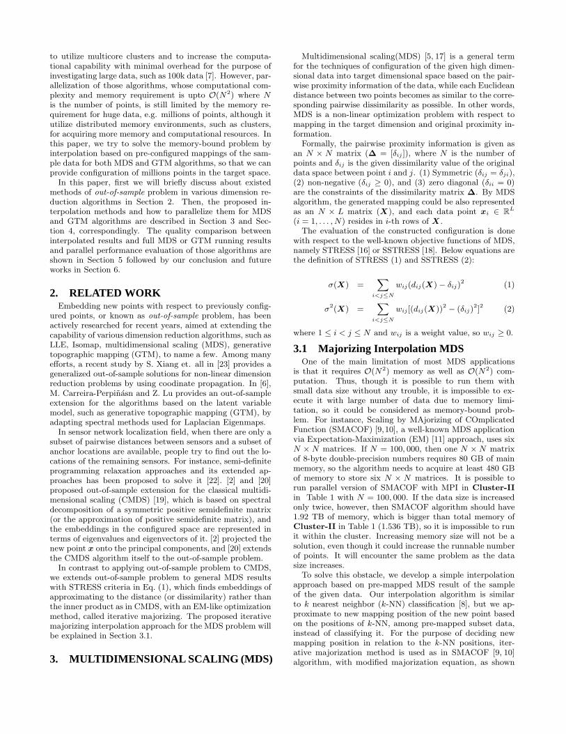
to utilize multicore clusters and to increase the computa-tional capability with minimal overhead for the purpose ofinvestigating large data, such as 100k data [7]. However, par-allelization of those algorithms, whose computational com-plexity and memory requirement is upto O(N2) where Nis the number of points, is still limited by the memory re-quirement for huge data, e.g. millions of points, although itutilize distributed memory environments, such as clusters,for acquiring more memory and computational resources. Inthis paper, we try to solve the memory-bound problem byinterpolation based on pre-configured mappings of the sam-ple data for both MDS and GTM algorithms, so that we canprovide configuration of millions points in the target space.
In this paper, first we will briefly discuss about existedmethods of out-of-sample problem in various dimension re-duction algorithms in Section 2. Then, the proposed in-terpolation methods and how to parallelize them for MDSand GTM algorithms are described in Section 3 and Sec-tion 4, correspondingly. The quality comparison betweeninterpolated results and full MDS or GTM running resultsand parallel performance evaluation of those algorithms areshown in Section 5 followed by our conclusion and futureworks in Section 6.
2. RELATED WORKEmbedding new points with respect to previously config-
ured points, or known as out-of-sample problem, has beenactively researched for recent years, aimed at extending thecapability of various dimension reduction algorithms, such asLLE, Isomap, multidimensional scaling (MDS), generativetopographic mapping (GTM), to name a few. Among manyefforts, a recent study by S. Xiang et. all in [23] provides ageneralized out-of-sample solutions for non-linear dimensionreduction problems by using coodinate propagation. In [6],M. Carreira-Perpinasn and Z. Lu provides an out-of-sampleextension for the algorithms based on the latent variablemodel, such as generative topographic mapping (GTM), byadapting spectral methods used for Laplacian Eigenmaps.
In sensor network localization field, when there are only asubset of pairwise distances between sensors and a subset ofanchor locations are available, people try to find out the lo-cations of the remaining sensors. For instance, semi-definiteprogramming relaxation approaches and its extended ap-proaches has been proposed to solve it [22]. [2] and [20]proposed out-of-sample extension for the classical multidi-mensional scaling (CMDS) [19], which is based on spectraldecomposition of a symmetric positive semidefinite matrix(or the approximation of positive semidefinite matrix), andthe embeddings in the configured space are represented interms of eigenvalues and eigenvectors of it. [2] projected thenew point x onto the principal components, and [20] extendsthe CMDS algorithm itself to the out-of-sample problem.
In contrast to applying out-of-sample problem to CMDS,we extends out-of-sample problem to general MDS resultswith STRESS criteria in Eq. (1), which finds embeddings ofapproximating to the distance (or dissimilarity) rather thanthe inner product as in CMDS, with an EM-like optimizationmethod, called iterative majorizing. The proposed iterativemajorizing interpolation approach for the MDS problem willbe explained in Section 3.1.
3. MULTIDIMENSIONAL SCALING (MDS)
Multidimensional scaling(MDS) [5, 17] is a general termfor the techniques of configuration of the given high dimen-sional data into target dimensional space based on the pair-wise proximity information of the data, while each Euclideandistance between two points becomes as similar to the corre-sponding pairwise dissimilarity as possible. In other words,MDS is a non-linear optimization problem with respect tomapping in the target dimension and original proximity in-formation.
Formally, the pairwise proximity information is given asan N × N matrix (Δ = [δij ]), where N is the number ofpoints and δij is the given dissimilarity value of the originaldata space between point i and j. (1) Symmetric (δij = δji),(2) non-negative (δij ≥ 0), and (3) zero diagonal (δii = 0)are the constraints of the dissimilarity matrix Δ. By MDSalgorithm, the generated mapping could be also representedas an N × L matrix (X), and each data point xi ∈ R
L
(i = 1, . . . , N) resides in i-th rows of X .The evaluation of the constructed configuration is done
with respect to the well-known objective functions of MDS,namely STRESS [16] or SSTRESS [18]. Below equations arethe definition of STRESS (1) and SSTRESS (2):
σ(X) =∑
i<j≤N
wij(dij(X) − δij)2 (1)
σ2(X) =∑
i<j≤N
wij [(dij(X))2 − (δij)2]2 (2)
where 1 ≤ i < j ≤ N and wij is a weight value, so wij ≥ 0.
3.1 Majorizing Interpolation MDSOne of the main limitation of most MDS applications
is that it requires O(N2) memory as well as O(N2) com-putation. Thus, though it is possible to run them withsmall data size without any trouble, it is impossible to ex-ecute it with large number of data due to memory limi-tation, so it could be considered as memory-bound prob-lem. For instance, Scaling by MAjorizing of COmplicatedFunction (SMACOF) [9,10], a well-known MDS applicationvia Expectation-Maximization (EM) [11] approach, uses sixN × N matrices. If N = 100, 000, then one N × N matrixof 8-byte double-precision numbers requires 80 GB of mainmemory, so the algorithm needs to acquire at least 480 GBof memory to store six N × N matrices. It is possible torun parallel version of SMACOF with MPI in Cluster-IIin Table 1 with N = 100, 000. If the data size is increasedonly twice, however, then SMACOF algorithm should have1.92 TB of memory, which is bigger than total memory ofCluster-II in Table 1 (1.536 TB), so it is impossible to runit within the cluster. Increasing memory size will not be asolution, even though it could increase the runnable numberof points. It will encounter the same problem as the datasize increases.
To solve this obstacle, we develop a simple interpolationapproach based on pre-mapped MDS result of the sampleof the given data. Our interpolation algorithm is similarto k nearest neighbor (k-NN) classification [8], but we ap-proximate to new mapping position of the new point basedon the positions of k-NN, among pre-mapped subset data,instead of classifying it. For the purpose of deciding newmapping position in relation to the k-NN positions, iter-ative majorization method is used as in SMACOF [9, 10]algorithm, with modified majorization equation, as shown
in below. The algorithm proposed in this section is calledMajorizing Interpolation MDS (MI-MDS).
The proposed algorithm is implemented as follows. We aregiven N data in high-dimensional space, say D-dimension,and proximity information (Δ = [δij ]) of those data as inSection 3. Among N data, the configuration of the n samplepoints in L-dimensional space, x1, . . . , xn ∈ R
L, called X,are already constructed by an MDS algorithm, here we useSMACOF algorithm. Then, we select k nearest neighbors,p1, . . . , pk ∈ P , of the given new point among n pre-mappedpoints with respect to corresponding δix, where x representsthe new point. Finally, the new mapping of the given newpoint x ∈ R
L is calculated based on the pre-mapped positionof selected k-NN and corresponding proximity informationδix. The finding new mapping position is considered as aminimization problem of STRESS (1) as similar as normalMDS problem with m points, where m = k + 1. However,only one point x is movable among m points, so we cansummarize STRESS (1) as belows, and we set wij = 1, for∀i, j in order to simplify.
σ(X) =∑
i<j≤N
(dij(X) − δij)2 (3)
= C +k∑
i=1
d2ix − 2
k∑i=1
δixdix (4)
where δix is the original dissimilarity value between pi andx, dix is the Euclidean distance in L-dimension between pi
and x, and C is constant part. The second term of Eq. (4)can be deployed as following:
k∑i=1
d2ix = ‖x − p1‖2 + · · · + ‖x − pk‖2 (5)
= k‖x‖2 +k∑
i=1
‖pi‖2 − 2xtq (6)
where qt = (∑k
i=1 pi1, . . . ,∑k
i=1 piL) and pij represents j-thelement of pi. In order to establish majorizing inequality,we apply Cauchy-Schwarz inequality to −dix of the thirdterm of Eq. (4). Please, refer to chapter 8 in [5] for detailsof how to apply Cauchy-Schwarz inequality to −dix. Sincedix = ‖pi − x‖, −dix could have following inequality basedon Cauchy-Schwarz inequality:
−dix ≤∑L
a=1(pia − xa)(pia − za)
diz(7)
=(pi − x)t(pi − z)
diz(8)
where zt = (zi, . . . , zL) and diz = ‖pi − z‖. The equality inEq. (7) occurs if x and z are equal. If we apply Eq. (8) tothe third term of Eq. (4), then we obtain
−k∑
i=1
δixdix ≤ −k∑
i=1
δix
diz(pi − x)t(pi − z) (9)
= −xtk∑
i=1
δix
diz(z − pi) + Cρ (10)
where Cρ is a constant. If Eq. (6) and Eq. (10) are appliedto Eq. (4), then it could be like following:
σ(X) = C +
k∑i=1
d2ix − 2
k∑i=1
δixdix (11)
≤ C + k‖x‖2 − 2xtq +k∑
i=1
‖pi‖2
− xtk∑
i=1
δix
diz(z − pi) + Cρ (12)
= τ (x, z) (13)
where both C and Cρ are constants. In the Eq. (13), τ (x, z),a quadratic function of x, is a majorization function of theSTRESS. Through setting the derivative of τ (x, z) equal tozero, we can obtain minimum of it; that is
∇τ (x, z) = 2kx − 2q − 2k∑
i=1
δix
diz(z − pi) = 0 (14)
x =q +
∑ki=1
δixdiz
(z − pi)
k(15)
where qt = (∑k
i=1 pi1, . . . ,∑k
i=1 piL), pij represents j-th el-ement of pi, and k is the number of nearest neighbor weselected.
The advantage of the iterative majorization algorithm isthat it guarantees to produce a series of mapping with non-increasing STRESS value as proceeds, which results in lo-cal minima. It is good enough to find local minima, sincethe proposed MI algorithm simplifies the complicated non-linear optimization problem as a small non-linear optimiza-tion problem, such as k + 1 points non-linear optimizationproblem, where k � N . Finally, if we substitute z withx[t−1] in Eq. (15), then we generate an iterative majorizingequation like following:
x[t] =q +
∑ki=1
δixdiz
(x[t−1] − pi)
k(16)
x[t] = p +1
k
k∑i=1
δix
diz(x[t−1] − pi) (17)
where diz = ‖pi − x[t−1]‖ and p is the average of k-NN’smapping results. Eq. (17) is an iterative equation usedto embed newly added point into target-dimensional space,based on pre-mapped positions of k-NN. The iteration stopcondition is essentially same as that of SMACOF algorithm,which is
Δσ(S[t]) = σ(S[t−1]) − σ(S[t]) < ε, (18)
where S = P ∪ {x} and ε is the given threshold value.Process of the out-of-sample MDS could be summarized
as following steps: (1) Sampling, (2) Running MDS withsample data, and (3) Interpolating the remain data pointsbased on the mapping results of the sample data.
The summary of proposed MI algorithm for interpolationof a new data, say x, in relation to pre-mapping result of thesample data is described in Alg. 1. Note that the algorithmuses p as an initial mapping of the new point x[0] unless
Algorithm 1 Majorizing Interpolation (MI) algorithm
1: Find k-NN: find k nearest neighbors of x, pi ∈ Pi = 1, . . . , k of the given new data based on originaldissimilarity δix.
2: Gather mapping results in target dimension of the k-NN.3: Calculate p, the average of pre-mapped results of pi ∈
P .4: Generate initial mapping of x, called x[0], either p or a
random point.5: Compute σ(S[0]), where S[0] = P ∪ {x[0]}.6: while t = 0 or (Δσ(S[t]) > ε and t ≤ MAX ITER) do7: increase t by one.8: Compute x[t] by Eq. (17).
9: Compute σ(S[t]).10: end while
11: return x[t];
initialization with p makes dix = 0, since the mapping isbased on the k-NN. If p makes dix = 0 (i = 1, . . . , k), thenwe use a random generated point as an initial position ofx[0].
3.2 Parallel MI-MDS AlgorithmSuppose that, among N points, mapping results of n sam-
ple points in the target dimension, say L-dimension, aregiven so that we could use those pre-mapped results of npoints via MI algorithm which is described above to em-bed the remaining points (M = N − n). Though interpo-lation approach is much faster than full running MDS algo-rithm, i.e. O(Mn + n2) vs. O(N2), implementing parallelMI algorithm is essential, since M can be still huge, likemillions. In addition, most of clusters are now in formsof multicore-clusters after multicore-chip invented, so weare using hybrid-model parallelism, which combine processesand threads together.
In contrast to the original MDS algorithm that the map-ping of a point is influenced by the other points, interpo-lated points are totally independent one another, except se-lected k-NN in the MI-MDS algorithm, and independency ofamong interpolated points let the MI-MDS algorithm to bepleasingly-parallel. In other words, there must be minimumcommunication overhead and load-balance can be achievedby using modular calculation to assign interpolated pointsto each parallel unit, either between processes or betweenthreads, as the number of assigned points are different atmost one each other.
Although interpolation approach itself is in O(Mn), if wewant to evaluate the quality of the interpolated results bySTRESS criteria in Eq. (1) of overall N points, it requiresO(N2) computation. Note that we implement our hybrid-parallel MI-MDS algorithm as each process has access toonly a subset of M interpolated points, without loss of gen-erality M/p points, as well as the information of all pre-mapped n points. It is natural way of using distributed-memory system, such as cluster systems, to access only sub-set of huge data which spread to over the clusters, so thateach process needs to communicate each other for the pur-pose of accessing all necessary data to compute STRESS.
3.3 Parallel Pairwise Computation with Sub-set of Data
p1
p5
p4
p3
p2
p5p4p3p2p1
p1
p2
p3
p4
p5p1
p2
p3
p4
p5
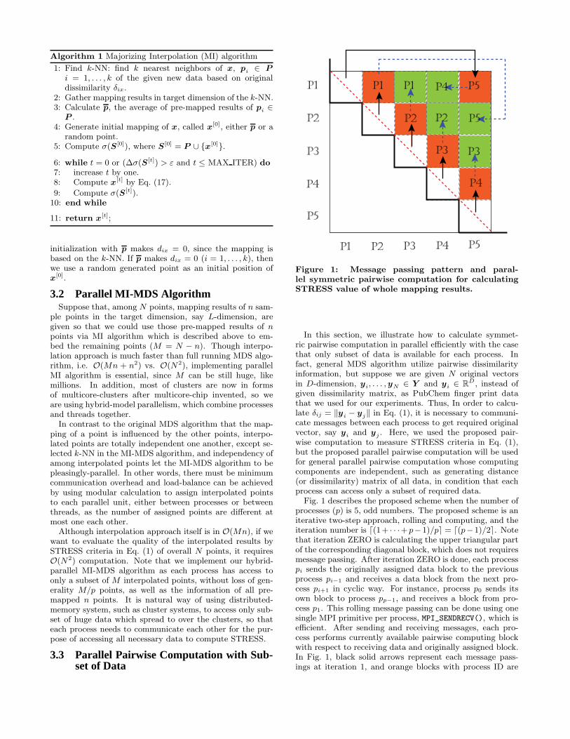
Figure 1: Message passing pattern and paral-lel symmetric pairwise computation for calculatingSTRESS value of whole mapping results.
In this section, we illustrate how to calculate symmet-ric pairwise computation in parallel efficiently with the casethat only subset of data is available for each process. Infact, general MDS algorithm utilize pairwise dissimilarityinformation, but suppose we are given N original vectorsin D-dimension, yi, . . . , yN ∈ Y and yi ∈ R
D, instead ofgiven dissimilarity matrix, as PubChem finger print datathat we used for our experiments. Thus, In order to calcu-late δij = ‖yi − yj‖ in Eq. (1), it is necessary to communi-cate messages between each process to get required originalvector, say yi and yj . Here, we used the proposed pair-wise computation to measure STRESS criteria in Eq. (1),but the proposed parallel pairwise computation will be usedfor general parallel pairwise computation whose computingcomponents are independent, such as generating distance(or dissimilarity) matrix of all data, in condition that eachprocess can access only a subset of required data.
Fig. 1 describes the proposed scheme when the number ofprocesses (p) is 5, odd numbers. The proposed scheme is aniterative two-step approach, rolling and computing, and theiteration number is (1+ · · ·+p−1)/p� = (p−1)/2�. Notethat iteration ZERO is calculating the upper triangular partof the corresponding diagonal block, which does not requiresmessage passing. After iteration ZERO is done, each processpi sends the originally assigned data block to the previousprocess pi−1 and receives a data block from the next pro-cess pi+1 in cyclic way. For instance, process p0 sends itsown block to process pp−1, and receives a block from pro-cess p1. This rolling message passing can be done using onesingle MPI primitive per process, MPI_SENDRECV(), which isefficient. After sending and receiving messages, each pro-cess performs currently available pairwise computing blockwith respect to receiving data and originally assigned block.In Fig. 1, black solid arrows represent each message pass-ings at iteration 1, and orange blocks with process ID are

Algorithm 2 Parallel Pairwise Computation
1: input: Y = a subset of data;2: input: p = the number of process;3: rank ⇐ the rank of process;4: sendTo ⇐ (rank − 1) mod p5: recvFrom ⇐ (rank + 1) mod p6: k ⇐ 0;7: Compute upper triangle in the diagonal blocks in Fig. 1;8: MAX ITER ⇐ (p − 1)/2�9: while k < MAX ITER do
10: k ⇐ k + 1;11: if k = 1 then12: MPI_SENDRECV(Y , sendTo, Y r, recvFrom);13: else14: Y s ⇐ Y r;15: MPI_SENDRECV(Y s, sendTo,Y r, recvFrom);16: end if
17: Do Computation();18: end while
the calculated blocks by the corresponding named processat iteration 1. From iteration 2 to iteration (p− 1)/2�, theabove two-steps are done repeatedly and the only differenceis nothing but sending received data block instead of theoriginally assigned data block. The green blocks and dottedblue arrows show the iteration 2 which is the last iterationfor the case of p = 5.
Also, for the case that the number of processes is even,the above two-step scheme works in high efficiency. Theonly difference between odd number case and even numbercase is that two processes are assigned to one block at thelast iteration of even number case, but not in odd numbercase. Though two processes are assigned to single block, itis easy to achieve load balance by dividing two section ofthe block and assign them to each process. Therefore, bothodd number processes and even number processes cases areparallelized well using the above rolling-computing scheme,with minimal message passing overhead. The summary ofthe above parallel pairwise computation is shown in Alg. 2.
4. GENERATIVE TOPOGRAPHIC MAPPINGThe Generative Topographic Mapping (GTM) algorithm
has been developed to find an optimal representation ofhigh-dimensional data in the low-dimensional space, or alsoknown as latent space. Unlike the well-known PCA-baseddimension reduction which finds linear embeddings in thetarget space, the GTM algorithm seeks a non-linear map-pings in order to provide more improved separations thanPCA [4]. Also, in contrast to Self-Organized Map (SOM)which finds lower dimensional representations in a heuristicapproach with no explicit density model for data, the GTMalgorithm finds a specific probability density based on Gaus-sian noise model. For this reason, GTM is often called as aprincipled alternative to SOM [3].
In GTM algorithm, one seeks a non-linear mapping ofuser-defined K points {zi}K
i=1 in the latent space to the orig-inal data space for N data points in a way K data pointscan optimally represent N data points {xj}N
j=1 in the high-dimensional space. More specifically, the GTM algorithmfinds a non-linear mapping f(zi; W ) with a weight parame-
ter set W and a coefficient β which maximize the followinglog-likelihood:
L(W , β) =
N∑j=1
ln
{1
K
K∑i=1
N (xj |f(zi; W ), β)
}, (19)
where N (xj |yi, β) represents Gaussian probability centeredon yi with variance β−1 (known as precision).
This problem is a variant of well-known K-clustering prob-lem which is NP-hard [1]. To solve the probem, GTM algo-rithm uses Expectation-Maximized (EM) method to find alocal optimal solution. Since the details of GTM algorithmis out of this paper’s scope, we recommend readers to referto the original GTM papers [3,4] for more details.
Once found an optimal parameter set in the GTM algo-rithm, we can draw a GTM map (also known as posteriormean projection plot) for N data points in the latent spaceby using the following equation:
〈xj〉 =K∑
i=1
rijzi (20)
where rij is the posterior probabilities, called responsibili-ties, defined by
rij =N (xj |yi, β)∑K
i′=1 N (xj |yi′ , β). (21)
for yi = f(zi; W )
4.1 GTM InterpolationThe core of GTM algorithm is to find the best K repre-
sentations for N data points, which makes the problem com-plexity is O(KN). Since in general K � N , the problem issub O(N2) which is the case in MDS problem. However, forlarge N the computations in GTM algorithm is still chal-lenging. For example, to draw a GTM map for 0.1 million166-dimensional data points in a 20x20x20 latent grid space,in our rough estimation it took about 30 hours by using 64cores.
To reduce such computational burden, we can use inter-polation approach in GTM algorithm, in which one can findthe best K representations from a portion of N data points,known as samples, instead of processing full N data pointsand continue to process remaining or out-of-sample data byusing the information learned from previous samples. Typi-cally, since the latter (interpolation process) doesn’t involvecomputationally expensive learning processes, one can re-duce overall execution time compared to the time spent forthe full data processing approach.
Although many researches have been performed to solvevarious non-linear manifold embeddings, including GTM al-gorithm, with this out-of-sample approach, we have chosena simple approach since it works well for our dataset usedin this paper. For more sophisticated and complexed data,one can see [6,14,23].
With a simple interpolation approach, we can perform theGTM process as follows:
1. Sampling – randomly select a sample set S = {sk}N′k=1
of size N ′ from the full dataset {xj}Nj=1 of size N ,
where sk, xj ∈ RD.
2. GTM process – perform GTM algorithm and find anoptimal K cluster center {yi}K
i=1 and a coefficient β for

R11
R21
R12 R13
R23R22
X1 X2 X3
Y1
Y2
Figure 2: An example of decomposition in GTMinterpolation for computing responsibility matrix Rin parallel by using a 2x3 virtual processor grid.
the sample set S. Let Y ∈ RK×D denote the matrix
representation of K centers, where i-th row containsyi ∈ R
D.
3. Compute responsibility – for the remaining dataset{tn}M
n=1 of size M = N − N ′, denoted by T , computea K × M pairwise distance matrix D where (i, j)-thelement dij is a Gaussian probability between tj andyi with variance β−1, which was learned from the sam-ples, such as dij = N (tj |yi, β). Compute a responsi-bility matrix R by , as follows:
R = D � (eetD) (22)
where a vector e = (1, ..., 1)t ∈ RK and � represents
element-wise division.
4. Interpolated map – by using Eq. (20), an interpo-lated GTM map Z, known as posterior mean plot, canbe computed by the following equation:
Z = RtZ (23)
where Z denotes the matrix represents of the latentpoints {zk}K
k=1.
In the GTM interpolation, computing responsibility ma-trix R (step 3) is the most time and memory consuming step.This step can be parallelized by decomposing the probleminto P-by-Q sub blocks such that total PQ processes canconcurrently process each block which approximately holds1/PQ elements of R. This is the same method used in par-allel GTM implementation discussed in [7]. More detailedalgorithm and analysis will be discussed in Section 4.2
4.2 Parallel GTM InterpolationThe core of parallel GTM interpolation is how to paral-
lelize the computations for the responsibility matrix R asin (22) since its computation is the most time and memoryconsuming task. This can be done by the same approach forthe general parallel matrix multiplication methods known asFox algorithm [13] and SUMMA [21] but with extra tasks.
Assuming that we have P ×Q virtual compute grids withtotal p = PQ processes, we can decompose the responsibilitymatrix R into P × Q sub blocks so that (u, v)-th sub blockof R, denoted by Ruv for u = 1, ..., P and v = 1, ..., Q, canbe computed by one process. For this computation, we alsoneed to decompose the matrix Y for K cluster centers intoP sub blocks such that each block contains approximatelyK/P cluster centers and divide the M out-of-sample dataT into Q sub blocks that one block contains approximately
M/Q out-of-sample data. Then, we can compute (i, n)-thsub block of R as follows:
Ruv = resp(Y u, T v) (24)
where resp(·, ·) is a function for computing responsibility andY u and T v are inputs, denoted by u-th and v-th sub blockof Y and T respectively.
A sketch of parallel GTM interpolation is as follows:
1. Broadcast sub-block {Y u}Pu=1 and {Zu}P
u=1 to P rank-
one node in rows and {T v}Qv=1 to each rank-one node
in columns of the P × Q grid respectively.
2. The rank-one node broadcast sub-block {Y u}Pu=1 and
{Zu}Pu=1 to row members and {T v}Q
v=1 to its columnmembers respectively.
3. (u, v)-th node computes sub distance matrix Duv byusing Y u and T v.
4. Collect P vectors {du}Pu=1 contains column sum of
Duv from column members and compute Ruv by
Ruv = Duv � e
P∑u
(du)t (25)
where a vector e = (1, ..., 1)t ∈ RK/P and � representselement-wise division.
5. (u, v)-th node computes the following sub block for theposterior mean Zuv
Zuv = (Ruv)tZuv (26)
and send to the rank-one node in columns. Then, v-thsub block of GTM map Z for N/Q data points is
Zv =P∑u
Zuv (27)
In our parallel GTM interpolation algorithm, main com-putation time is spent in computing K/P × N/Q distancematrix Duv which requires approximately O(KN/PQ)τC
computation time, where τC represents a unit time for ba-sic operations such as multiplication and summation. Re-garding the time spent for communication, our algorithmconsumes time due to the network bandwidth, denote τB,which increases as the size of data to send and receive. As-suming a minimum spanning tree broadcasting and collect-ing operations, our algorithm will spend O(log P (KD/Q +N/Q + KN/PQ) + log P (KD/P + KL/P ))τB . Also, as weincrease P or Q, an overhead can occur due to the networklatency, denote τL, which mainly occurs due to the numberof communications. In our parallel GTM interpolation, wehave O(2P + Q) communications. Since generally L � Dand those are constant, we can formulate the total comput-ing time T (K,N, P, Q) in our algorithm, with respect to Klatent points, N data points, and P×Q processes, as follows:
O(
KN
PQ
)τC + O(2P + Q)τL
+O(
log P
(N
Q+
KN
PQ
)+ log Q
(KD
P
))τB (28)
where τC , τB, and τL represents unit time for computation,network bandwidth, and network latency respectively.

Since the running time with no parallelization T1 = O(KN),we can expect the speed up as S(K, N, P, Q) = T1/T (K, N, P, Q)and its corresponding efficiency E(K, N, P, Q) = S(K, N, P, Q)/PQas follows.{
1 + O(
log P
KPQ2+
log P
P 2Q2+
log Q
NP 2Q
)τB + O
(2P + Q
PQ
)τL
}−1
(29)
The above equation implies the following: in the casewhere P and Q are large enough but network latency dueto τL is negligibly small, we can achieve an ideal efficiencyE(K, N, P, Q) = 1. However, as we increase the number ofcores, the efficiency of our algorithm will be hurt due to theincrease number of communications. Our experiment resultssupport this expectation.
5. ANALYSIS OF EXPERIMENTAL RESULTSTo measure the quality and parallel performance of our
MDS and GTM with interpolation approach discussed inthis paper, we have used 166-dimensional chemical datasetobtained from PubChem project database1, which is a NIH-funded repository for over 60 million chemical molecules andprovides their chemical structures and biological activities,for the purpose of chemical information mining and explo-ration. In this paper we have used randomly selected up to4 million chemical subsets for our testing. The computingclusters we have used in our experiments are summarized inTable 1.
In the following, we will mainly show i) the quality of ourinterpolation approaches in performing MDS and GTM algo-rithms, with respect to various sample sizes – 12.5k, 25k, and75k randomly selected from 100k dataset as a basis, and ii)performance measurement of our parallelized interpolationalgorithms on our clustering systems as listed in Table 1, andfinally, iii) our results on processing up to 4 million MDS andGTM maps based on the trained result from 100K dataset.
5.1 Mapping Quality Comparison
5.1.1 MDS vs. MI-MDSGenerally, the quality of k-NN (k-nearest neighbor) clas-
sification (or regression) is related to the number of neigh-bors. For instance, if we choose larger number for the k,then the algorithm shows higher bias but lower variance.On the other hands, the k-NN algorithms show lower biasbut higher variance with respect to smaller number of neigh-bors. The purpose of the MI algorithm is to find appropriateembeddings for the new points based on the given mappingsof the sample data, so it is better to be sensitive to the map-pings of the k-NN of the new point than to be stable withrespect to the mappings of whole sample points. Thus, inthis paper, the authors use 2-NN for the MI algorithm.
Fig. 3 shows the comparison of quality between interpo-lated results upto 100K data with different sample size databy using 2-NN and MDS (SMACOF) only result with 100kpubchem data. The y-axis of the plot is STRESS (1) nor-malized with
∑i<j δ2
ij , and the difference between MDS onlyresults and interpolated with 50k is only around 0.004. Evenwith small portion of sample data (12.5k data is only 1/8of 100k), the proposed MI algorithm produces good enoughmapping in target dimension using very smaller amount oftime than when we run MDS with full 100k data. Fig. 4
1PubChem,http://pubchem.ncbi.nlm.nih.gov/
Sample size
ST
RE
SS
0.00
0.02
0.04
0.06
0.08
0.10
2e+04 4e+04 6e+04 8e+04 1e+05
Algorithm
MDS
INTP
Figure 3: Quality comparison between Interpolatedresult upto 100k based on the sample data and 100kMDS result
Sample size
Ela
psed
tim
e (s
ec)
0
5
10
15
20
12.5k 25k 50k
Algorithm
INTP
Figure 4: Elapsed time of parallel MI-MDS runningtime upto 100k data with respect to the sample sizeusing 16 nodes of the Cluster-II in Table 1. Notethat the computational time complexity of MI-MDSis O(Mn) where n is the sample size and M = N − n.
shows the MI-MDS running time with respect to the sampledata using 16 nodes of the Cluster-II in Table 1. Note thatthe full MDS running time with 100k using 16 nodes of theCluster-II in Table 1 is around 27006 sec.
Above we discussed about the MI-MDS quality of the fixedtotal number (100k) and with respect to the different sam-ple data size, compared to MDS running result with totalnumber of data (100k). Now, the opposite direction of test,which tests scalability of the proposed interpolation algo-

Table 1: Compute cluster systems used for the performance analysisFeatures Cluster-I Cluster-II
# Nodes 8 32
CPU AMD Opteron 8356 2.3GHz Intel Xeon E7450 2.4 GHz
# CPU / # Cores per node 4 / 16 4 / 24
Total Cores 128 768
Memory per node 16 GB 48 GB
Network Giga bit Ethernet 20 Gbps Infiniband
Operating System Windows Server 2008 HPC Edition (Ser-vice Pack 2) - 64 bit
Windows Server 2008 HPC Edition (Ser-vice Pack 2) - 64 bit
Total size
ST
RE
SS
0.00
0.02
0.04
0.06
0.08
0.10
500000 1000000 1500000 2000000
Figure 5: STRESS value change of Interpolationlarger data, such as 1M and 2M data points, with100k sample data. The initial STRESS value of MDSresult of 100k data is 0.0719.
rithm, is performed as following: we fix the sample datasize to 100k, and the interpolated data size is increasedfrom one millions (1M) to four millions (4M). Then, theSTRESS value is measured for each running result of totaldata, i.e. 1M + 100k, 2M + 100k, and so on. The measuredSTRESS value is shown in Fig. 5. There are some qualitylost between the full MDS running result with 100k dataand the 1M interpolated results based on that 100k map-ping, which is about 0.007 difference in normalized STRESScriteria. However, there is no much difference between the1M interpolated result and 2M interpolated result, althoughthe sample size is quite small portion of total data and theout-of-sample data size increases as twice. From the aboveresult, we could consider that the proposed MI-MDS algo-rithm works well and scalable if we are given a good enoughpre-configured result which represents well the structure ofthe given data. Note that it is not possible to run SMACOFalgorithm with only 200k data points due to memory bound,within the systems in Table 1.
5.1.2 GTM vs. Interpolated-GTMTo measure the quality of GTM interpolation algorithm,
we have compared quality of GTM maps, generated by us-
Sample SizeN
egat
ive
log−
likel
ihoo
d pe
r po
int
32
33
34
35
36
12.5k 25k 50k 100k
Algorithm
GTM
INTP
Figure 6: Comparison of maximum log-likelihoodfrom GTM with full-dataset processing without in-terpolation (GTM) and the GTM with interpola-tion approach (INTP) with various sampling sizes –12.5k, 25k, and 50k – for 100k PubChem dataset.As the sample size increases, INTP finds very closeresults with GTM.
ing the full GTM processing with no interpolation (hereafterGTM for short) versus maps by using the interpolation ap-proach (hereafter INTP for short) with various sample sizes(12.5k, 25k, and 50k) in terms of maximum log-likelihood(a large maximum log-likelihood implies better quality ofmap), as defined in (19). Our test result is shown in Fig. 6where negative log-likelihood values are plotted for each testcase and thus points in lower area represent the better qual-ity. Our results show that the interpolation approach hasproduced almost the same quality of maps with the mapgenerated by using the full dataset. Also the result showsthat the interpolation with small sample sizes (12.5k) is the
worst performance case, while othersO results are quite closeto the out of full data processing case. This is the commoncase that small sample size can lead skewed interpretationof the full data.
Next, we compare GTM versus INTP (GTM with inter-polation) in terms of processing time. For this purpose, weprocessed up to 100k dataset with various sample sizes start-ing from 12.5k up to 50k and compare the processing timewith the case of no use of interpolation (full 100k dataset).Since the original GTM algorithm uses EM method in whicha local solution is found in an iterative fashion and the number of iterations is unpredictable, we have measured average

number of iterations for processing for the 100k dataset anduse this average to project GTM running time for process-ing 12.5k, 25k, and 50k dataset. By adding interpolationrunning time as we measured in the previous experiment,we have projected the total running time for using GTMinterpolation with various sampling sizes as shown in Fig.7. As we expected, the interpolation process doesOt involvecomputing-intensive training processes and thus processingtime is very short, compared with the approach of using fulldataset. By combining the results shown in Fig. 6 and Fig.7, we show that GTM interpolation can be used to producethe same quality of GTM maps with less computing time.
5.2 Parallel Performance
5.2.1 Parallel MI-MDSIn the above section, we discussed about the quality of
constructed configuration of MI-MDS based on the STRESSvalue of the interpolated configuration. Here, we would liketo investigate the MPI communication overhead and parallelperformance of the proposed parallel MI-MDS implementa-tion in terms of efficiency with respect to the running resultswithin Cluster-I and Cluster-II in Table 1.
First of all, we prefer to investigate the parallel overhead,specially MPI communication overhead which could be ma-jor parallel overhead for the parallel MI-MDS in Section 3.2.Parallel MI-MDS consists of two different computations, MIpart and STRESS calculation part. MI part is pleasinglyparallel and its computational complexity is O(M), whereM = N −n, if the sample size n is considered as a constant.Since the MI part uses only two MPI primitives, MPI_GATHERand MPI_BROADCAST, at the end of interpolation to gather allthe interpolated mapping results and spread out the com-bined interpolated mapping result to all the processes forthe further computation. Thus, the communicated messageamount through MPI primitives is O(M), so it is not depen-dent on the number of processes but the number of wholeout-of-sample points.
For the STRESS calculation part, that applied to the pro-posed symmetric pairwise computation in Section 3.3, eachprocess uses MPI_SENDRECV k times to send assigned blockor rolled block, whose size is M/p, where k = (p − 1)/2�for communicating required data and MPI_REDUCE twice forcalculating
∑i<j(dij − δij)
2 and∑
i<j δ2ij . Thus, the MPI
communicated data size is O(M/p × p) = O(M) withoutregard to the number of processes.
The MPI overhead during MI part and STRESS calculat-ing part at Cluster-I and Cluster-II in Table 1 are shownin Fig. 7 and Fig. 8, correspondingly. Note that the x-axisof both figures is the sample size (n) but not M = N −n. Inthe figures, the model is generated as O(M) starting withthe smallest sample size, here 12.5k. Both Fig. 7 and Fig. 8show that the actual overhead measurement follows the MPIcommunication overhead model.
Fig. 9 and Fig. 10 illustrate the efficiency of Interpola-tion part and STRESS calculation part of the parallel MI-MDS running results with different sample size - 12.5k, 25k,and 50k - with respect to the number of parallel units usingCluster-I and Cluster-II, correspondingly. Equations for theefficiency is following:
f =pT (p)− T (1)
T (1)(30)
Sample size
MP
I ove
rhea
d tim
e (s
ec)
0.5
1.0
1.5
2.0
2.5
15000 20000 25000 30000 35000 40000 45000 50000
Type
INTP_model
INTP_Ovhd
STR_model
STR_Ovhd
Figure 7: Parallel overhead modeled as due to MPIcommunication in terms of sample data size (m) us-ing Cluster-I in Table 1 and message passing over-head model.
Sample size
MP
I ove
rhea
d tim
e (s
ec)
0.4
0.6
0.8
1.0
15000 20000 25000 30000 35000 40000 45000 50000
Type
INTP_model
INTP_Ovhd
STR_model
STR_Ovhd
Figure 8: Parallel overhead modeled as due to MPIcommunication in terms of sample data size (m) us-ing Cluster-II in Table 1 and message passing over-head model.
ε =1
1 + f(31)
where p is the number of parallel units, T (p) is the runningtime with p parallel units, and T (1) is the sequential runningtime. In practice, Eq. (30) can be replaced with following:
f =αT (p1) − T (p2)
T (p2)(32)

Number of cores
Effi
cien
cy
0.0
0.2
0.4
0.6
0.8
1.0
1.2
24 24.5 25 25.5 26 26.5 27
Type
INTP_12.5k
INTP_25k
INTP_50k
STR_12.5k
STR_25k
STR_50k
Figure 9: Efficiency of Interpolation part andSTRESS evaluation part runtime in parallel MI-MDS application with respect to different sampledata size using Cluster-I in Table 1. Total data sizeis 100K.
where α = p1/p2 and p2 is the smallest number of used coresfor the experiment, so alpha ≥ 1. We use Eq. (32) for theoverhead calculation.
In Fig. 9, 16 to 128 cores are used to measure parallelperformance with 8 processes, and 32 to 384 cores are usedto evaluate the parallel performance of the proposed parallelMI-MDS with 16 processes in Fig. 10. Processes communi-cate via MPI primitives and each process is also parallelizedin thread level. Both Fig. 9 and Fig. 10 show very goodefficiency with appropriate degree of parallelism. Since bothMI part and STRESS calcualtion part are pleasingly paral-lel within a process, the major overhead portion is the MPImessage communicating overhead unless load balance is notachieved in thread-level parallelization within each process.In above, the MPI communicating overhead is investigatedand the MPI communicating overhead shows O(M) relation.Thus, the MPI overhead is constant if we examine with thesame number of process and the same out-of-sample datasize. Since the parallel computation time is decreased asmore cores are used, but the overhead time is constant, itlowers the efficiency as the number of cores is increased,as we expected. Note that the number of processes whichlowers the efficiency dramatically is different between theCluster-I and Cluster-II. The reason is that the MPI over-head time of Cluster-I is bigger than that of Cluster-II dueto different network environment, i.e. Giga bit ethernet and20Gbps Infiniband. The difference is easily found by com-paring Fig. 7 and Fig. 8.
5.2.2 Parallel GTM InterpolationWe have measured performance of our parallel GTM in-
terpolation algorithm discussed in 4.2 by using 16 nodes ofthe Cluster-II shown in Table 1, as we increase the numberof cores from 16 to 256.
As shown in (29), the ideal efficiency of our parallel GTM
Number of cores
Effi
cien
cy
0.0
0.2
0.4
0.6
0.8
1.0
1.2
25 25.5 26 26.5 27 27.5 28 28.5
Type
INTP_12.5k
INTP_25k
INTP_50k
STR_12.5k
STR_25k
STR_50k
Figure 10: Efficiency of Interpolation part andSTRESS evaluation part runtime in parallel MI-MDS application with respect to different sampledata size using Cluster-II in Table 1. Total data sizeis 100K.
Number of cores
Effi
cien
cy
0.0
0.2
0.4
0.6
0.8
1.0
16 32 64 128 256
Type
12.5k−Computation Only
12.5k−Overall
25k−Computation only
25k−Overall
50k−Computation only
50k−Overall
Figure 11: Efficiency of parallel GTM interpolationwith respect to various sample sizes (12.5k, 25k, and50k) and number of cores (from 32 up to 256 cores)
interpolation algorithm is constant as 1.0 with respect to thenumber of PQ processes and can be degraded due to the net-work latency which is mainly caused by the high number ofcommunications. As we increase the number of cores (moredecompositions), the communications between sub blocksare increasing and thus the network latency can affect theefficiencies.
As we expected, our experiment results shown in Fig. 12,the efficiency of our parallel GTM interpolation is close to
Sample size
Ela
psed
tim
e (s
ec)
6
8
10
12
14
12.5k 25k 50k
Algorithm
INTP
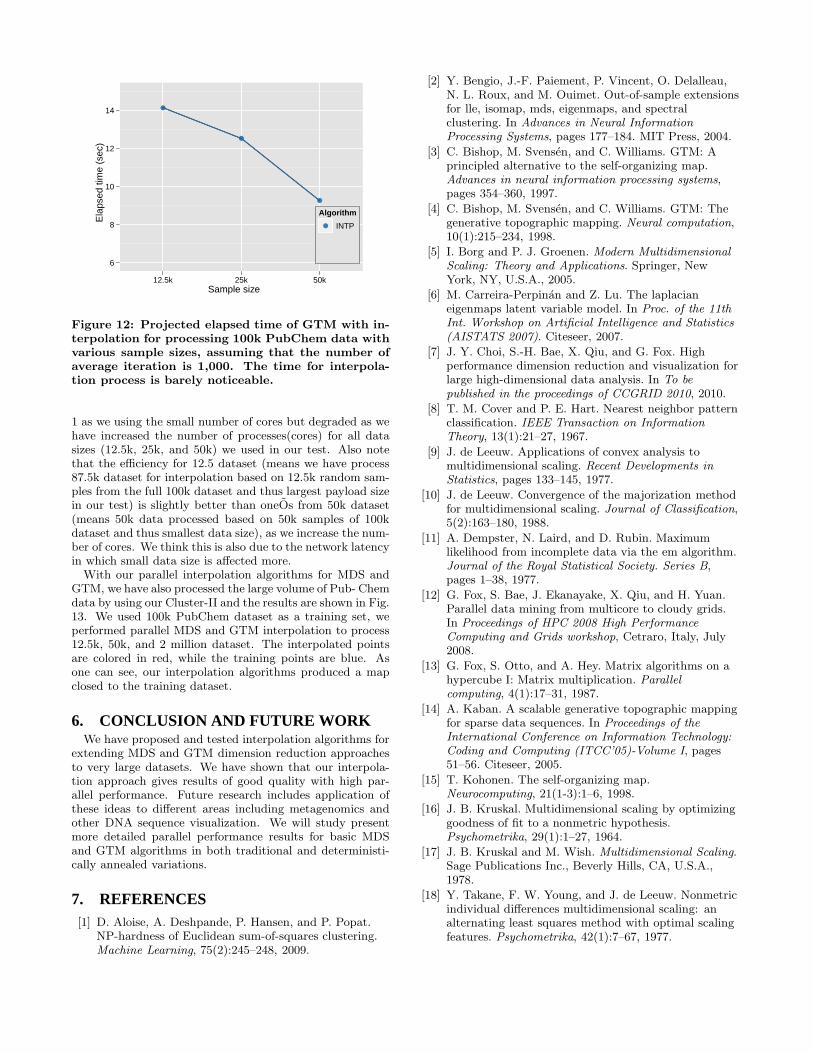
Figure 12: Projected elapsed time of GTM with in-terpolation for processing 100k PubChem data withvarious sample sizes, assuming that the number ofaverage iteration is 1,000. The time for interpola-tion process is barely noticeable.
1 as we using the small number of cores but degraded as wehave increased the number of processes(cores) for all datasizes (12.5k, 25k, and 50k) we used in our test. Also notethat the efficiency for 12.5 dataset (means we have process87.5k dataset for interpolation based on 12.5k random sam-ples from the full 100k dataset and thus largest payload sizein our test) is slightly better than oneOs from 50k dataset(means 50k data processed based on 50k samples of 100kdataset and thus smallest data size), as we increase the num-ber of cores. We think this is also due to the network latencyin which small data size is affected more.
With our parallel interpolation algorithms for MDS andGTM, we have also processed the large volume of Pub- Chemdata by using our Cluster-II and the results are shown in Fig.13. We used 100k PubChem dataset as a training set, weperformed parallel MDS and GTM interpolation to process12.5k, 50k, and 2 million dataset. The interpolated pointsare colored in red, while the training points are blue. Asone can see, our interpolation algorithms produced a mapclosed to the training dataset.
6. CONCLUSION AND FUTURE WORKWe have proposed and tested interpolation algorithms for
extending MDS and GTM dimension reduction approachesto very large datasets. We have shown that our interpola-tion approach gives results of good quality with high par-allel performance. Future research includes application ofthese ideas to different areas including metagenomics andother DNA sequence visualization. We will study presentmore detailed parallel performance results for basic MDSand GTM algorithms in both traditional and deterministi-cally annealed variations.
7. REFERENCES[1] D. Aloise, A. Deshpande, P. Hansen, and P. Popat.
NP-hardness of Euclidean sum-of-squares clustering.Machine Learning, 75(2):245–248, 2009.
[2] Y. Bengio, J.-F. Paiement, P. Vincent, O. Delalleau,N. L. Roux, and M. Ouimet. Out-of-sample extensionsfor lle, isomap, mds, eigenmaps, and spectralclustering. In Advances in Neural InformationProcessing Systems, pages 177–184. MIT Press, 2004.
[3] C. Bishop, M. Svensen, and C. Williams. GTM: Aprincipled alternative to the self-organizing map.Advances in neural information processing systems,pages 354–360, 1997.
[4] C. Bishop, M. Svensen, and C. Williams. GTM: Thegenerative topographic mapping. Neural computation,10(1):215–234, 1998.
[5] I. Borg and P. J. Groenen. Modern MultidimensionalScaling: Theory and Applications. Springer, NewYork, NY, U.S.A., 2005.
[6] M. Carreira-Perpinan and Z. Lu. The laplacianeigenmaps latent variable model. In Proc. of the 11thInt. Workshop on Artificial Intelligence and Statistics(AISTATS 2007). Citeseer, 2007.
[7] J. Y. Choi, S.-H. Bae, X. Qiu, and G. Fox. Highperformance dimension reduction and visualization forlarge high-dimensional data analysis. In To bepublished in the proceedings of CCGRID 2010, 2010.
[8] T. M. Cover and P. E. Hart. Nearest neighbor patternclassification. IEEE Transaction on InformationTheory, 13(1):21–27, 1967.
[9] J. de Leeuw. Applications of convex analysis tomultidimensional scaling. Recent Developments inStatistics, pages 133–145, 1977.
[10] J. de Leeuw. Convergence of the majorization methodfor multidimensional scaling. Journal of Classification,5(2):163–180, 1988.
[11] A. Dempster, N. Laird, and D. Rubin. Maximumlikelihood from incomplete data via the em algorithm.Journal of the Royal Statistical Society. Series B,pages 1–38, 1977.
[12] G. Fox, S. Bae, J. Ekanayake, X. Qiu, and H. Yuan.Parallel data mining from multicore to cloudy grids.In Proceedings of HPC 2008 High PerformanceComputing and Grids workshop, Cetraro, Italy, July2008.
[13] G. Fox, S. Otto, and A. Hey. Matrix algorithms on ahypercube I: Matrix multiplication. Parallelcomputing, 4(1):17–31, 1987.
[14] A. Kaban. A scalable generative topographic mappingfor sparse data sequences. In Proceedings of theInternational Conference on Information Technology:Coding and Computing (ITCC’05)-Volume I, pages51–56. Citeseer, 2005.
[15] T. Kohonen. The self-organizing map.Neurocomputing, 21(1-3):1–6, 1998.
[16] J. B. Kruskal. Multidimensional scaling by optimizinggoodness of fit to a nonmetric hypothesis.Psychometrika, 29(1):1–27, 1964.
[17] J. B. Kruskal and M. Wish. Multidimensional Scaling.Sage Publications Inc., Beverly Hills, CA, U.S.A.,1978.
[18] Y. Takane, F. W. Young, and J. de Leeuw. Nonmetricindividual differences multidimensional scaling: analternating least squares method with optimal scalingfeatures. Psychometrika, 42(1):7–67, 1977.

(a) MDS 12.5k (b) MDS 50k (c) GTM 2M
Figure 13: Interpolated MDS results based on 12.5k and 50k trained samples upto 100k data, and GTM mapfor 2M PubChem data based on the trained information from 100k samples. Points in red are trained dataand others are interpolated points.
[19] W. S. Torgerson. Multidimensional scaling: I. theoryand method. Psychometrika, 17(4):401–419, 1952.
[20] M. W. Trosset and C. E. Priebe. The out-of-sampleproblem for classical multidimensional scaling.Computational Statistics and Data Analysis,52(10):4635–4642, 2008.
[21] R. Van De Geijn and J. Watts. SUMMA: Scalableuniversal matrix multiplication algorithm.Concurrency Practice and Experience, 9(4):255–274,1997.
[22] Z. Wang, S. Zheng, Y. Ye, and S. Boyd. Furtherrelaxations of the semidefinite programming approachto sensor network localization. SIAM Journal onOptimization, 19(2):655–673, 2008.
[23] S. Xiang, F. Nie, Y. Song, C. Zhang, and C. Zhang.Embedding new data points for manifold learning viacoordinate propagation. Knowledge and InformationSystems, 19(2):159–184, 2009.