diion paper erieftp.iza.org/dp11948.pdfdiion paper erie iza dp no. 11948 carlywill sloan george...

DISCUSSION PAPER SERIES

IZA DP No. 11948

CarlyWill SloanGeorge NaufalHeather Caspers

The Effect of Risk Assessment Scores on Judicial Behavior and Defendant Outcomes

NOVEMBER 2018

Any opinions expressed in this paper are those of the author(s) and not those of IZA. Research published in this series may include views on policy, but IZA takes no institutional policy positions. The IZA research network is committed to the IZA Guiding Principles of Research Integrity.The IZA Institute of Labor Economics is an independent economic research institute that conducts research in labor economics and offers evidence-based policy advice on labor market issues. Supported by the Deutsche Post Foundation, IZA runs the world’s largest network of economists, whose research aims to provide answers to the global labor market challenges of our time. Our key objective is to build bridges between academic research, policymakers and society.IZA Discussion Papers often represent preliminary work and are circulated to encourage discussion. Citation of such a paper should account for its provisional character. A revised version may be available directly from the author.

Schaumburg-Lippe-Straße 5–953113 Bonn, Germany

Phone: +49-228-3894-0Email: [email protected] www.iza.org

IZA – Institute of Labor Economics

DISCUSSION PAPER SERIES

IZA DP No. 11948

The Effect of Risk Assessment Scores on Judicial Behavior and Defendant Outcomes

NOVEMBER 2018

CarlyWill SloanTexas A&M University

George NaufalTexas A&M University and IZA

Heather CaspersTexas A&M University

ABSTRACT

IZA DP No. 11948 NOVEMBER 2018

The Effect of Risk Assessment Scores on Judicial Behavior and Defendant Outcomes*

The use of risk assessment scores as a means of decreasing pretrial detention for low-risk,

primarily poor defendants is increasing rapidly across the United States. Despite this, there is

little evidence on how risk assessment scores alter criminal outcomes. Using administrative

data from a large county in Texas, we estimate the effect of a risk assessment score policy

on judge bond decisions, defendant pretrial detention, and pretrial recidivism. We identify

effects by exploiting a large, sudden policy change using a regression discontinuity design.

This approach effectively compares defendants booked just before and after the policy

change. Results show that adopting a risk assessment score leads to increased release on

non-financial bond and decreased pretrial detention. These results appear to be driven

by poor defendants. We also find risk assessment scores did not increase violent pretrial

recidivism, however there is some suggestive evidence of small increases in non-violent

pretrial recidivism.

JEL Classification: D81, K14, K42, L88

Keywords: pretrial detention, bail, risk assessment, recidivism, regression, discontinuity

Corresponding author:George NaufalPublic Policy Research InstituteTexas A&M University4476 TAMUCollege Station, TX 77843USA

E-mail: [email protected]

* We are grateful for useful comments from Mark Hoekstra, Brittany Street and Travis County Pretrial Services.

1 Introduction

In the United States (US), individuals are guaranteed by the Eighth Amendment the right

to reasonable bail and, therefore, the potential for release before trial. However, 34 percent

of all felony defendants, 90 percent of those pretrial detained, are not released because of

their inability to post monetary bail (Bureau of Justice Statistics, 2013). In response to the

overcrowding of prisons and a perception that the existing bail system disproportionately

harms the poor and those with low-risk, many jurisdictions are beginning to look for ways

to reduce their inmate population. Often suggested is a shift from monetary bail to a risk-

based system, where defendants are released according to their risk of recidivism instead of

their financial status. Assessing defendant risk is not a new idea in criminal justice, but in

recent years risk assessment has taken on the additional meaning of using more technical

and actuarial methods of predicting the likelihood of future crimes or failure to appear.

Supporters of risk assessment scores argue that assessing individuals based on their risk

rather than their income could lead to less pretrial detention, allowing defendants to keep

their jobs and imposing nearly zero costs on the criminal justice system if defendants do not

recidivate pretrial. These policies are also most likely to benefit low-income defendants who

cannot post bail. Opponents claim that increasing pretrial release through the use of non-

financial bond and risk assessment scores could increase pretrial crime, further threatening

societal safety and raising costs. This paper focuses on the question of whether the use of risk

assessment scores can increase non-financial bond, and decrease pretrial detention without

increasing societal costs.

Although the use of risk assessment scores is rapidly increasing across the United States,

2

there is little to no research on their causal effects on release patterns and defendant out-

comes. There are two primary difficulties with estimating the effect of risk assessment scores.

First, most jurisdictions do not keep detailed records on defendants from arrest until dispo-

sition, including recording whether they were assessed using a risk assessment score. Second,

some jurisdictions only evaluate certain defendant types, often those with less serious crimes,

using a risk assessment score. Any resulting cross-sectional comparisons would be biased as

those with scores are observably, and likely unobservably, different across many attributes.

We estimate the effect of risk assessment using data from Travis County, Texas, a large

county with a population of over 1.2 million (United States Census Bureau, 2017). On Jan-

uary 14th, 2013, Travis County abruptly changed from not using a research-based risk as-

sessment score at all to assigning one to nearly every inmate. Importantly, Travis County’s

implementation of the risk assessment score policy was immediate and the exact policy

change date was not announced. There was no slow roll-out of the policy—one day the

county assigned no risk assessment scores, and the following day it assigned scores to over

75 percent of defendants booked after arrest. This type of sudden change is ideal for identi-

fying local effects through a regression discontinuity design. Using the timing of the policy

change, we are able to compare defendants booked just before and after the policy change.

The identifying assumption is that all determinants of defendant outcomes aside from the

policy change vary smoothly through the policy change. Said another way, we assume that

defendants who choose to commit crimes on January 12th and 13th versus January 14th

and 15th are not meaningfully different except that those on the later dates received a risk

assessment score. We also show empirical tests using exogenous covariates that support this

3

assumption.

First, results show that the use of a risk assessment score increases release on non-financial

bail by 4.5%-7.5% and decreases pretrial detention by 7%-10%. We also provide evidence

that results are driven by low-income defendants. Second, we are able to rule out meaningful

increases in violent pretrial recidivism. These results are robust multiple inference and several

robustness checks. There is also some suggestive evidence that non-violent pretrial recidivism

may increase, however these results are not robust.

To our knowledge, this paper provides the first causal evidence on the effects of pretrial

risk assessment scores. As a result, our work contributes to multiple important existing lit-

eratures. First, we contribute to a small, but growing, literature on risk assessment scores in

general. The majority of this literature has focused on validity of risk assessment instruments

rather than a policy’s overall effect (Almond et al., 2017; Flores et al., 2017; Meredith et al.,

2007; Schmidt et al., 2017). For example, many states have validated their risk assessment

score use by documenting that higher scores are correlated with higher recidivism (Zhang

et al., 2014; DeMichele et al., 2018; Latessa et al., 2010; Turner et al., 2009 ). Others have

focused on comparing human decisions with actuarial predictions (Chanenson and Hyatt,

2016; Grove et al., 2000; Dressel and Farid, 2018). Perhaps the most rigorous paper in this

field, Kleinberg et al. (2017), used machine learning to determine crime rates would have

been if release decisions were made solely based on a risk assessment algorithm. They found

that if the same number of inmates were released, but according to their algorithmic risk

scores, crime rates would fall.

In contrast, there are few serious independent evaluations of risk assessment score im-

4

plementation. This paper is most similar in spirit to Stevenson (2018b). She evaluated

multiple pretrial risk assessment score policy changes in Kentucky using an event study

framework. In contrast to our causal estimates, Stevenson (2018b) provided rigorous pre-

and post-comparisons, concluding that the use of risk assessment scores alters bail-setting

behavior and leads to increases in failures-to-appear and pretrial crime.

Our paper also relates to a number of papers on the effects of pretrial detention on

defendant outcomes. In general, these papers have found that pretrial detention leads to an

increased likelihood of conviction (Dobbie et al., 2018; Stevenson, 2018a; Leslie and Pope,

2016; Didwania, 2018; Heaton et al., 2017). Others have considered the effect of nonmonetary

bail on outcomes, finding that nonmonetary bail decreases conviction rates (Gupta et al.,

2016).

The results of this paper have important implications for criminal justice actors and

defendants. First, our finding that risk assessment scores increase non-financial bail and

decrease pretrial detention suggests that this policy can be used to lower costs. These costs

could be substantial as the estimated annual cost of pretrial detention in the US is $13.4

billion (Wagner and Rabuy, 2017). Significantly, we also show that this reduction in pretrial

detention and increase in non-financial bail releases could be possible without increases in

violent pretrial recidivism.

Second, the use of risk assessment scores is important to defendants because it relieves

lower-income defendants of the potentially disproportionate burden of financial bail and

therefore pretrial detention. Perhaps most importantly, decreases in pretrial detention are

also associated with greater job stability, less reliance on government assistance, lower prob-

5

ability of conviction and less separation from family (Dobbie et al., 2018). At least to the

extent that our results apply in other settings, these findings indicate that risk assessment

score polices may be an effective tool for decreasing the income-based disparity in pretrial

detention and improving the lives of defendants. Notably, these increases in pretrial deten-

tion are not associated with increases in violent recidivism, implying minimal risk and costs

to society. However, policy makers must be careful to weigh these potential benefits with

the potential for some increases in non-violent recidivism.

2 Overview of the Travis County System

With a population of over 1.2 million, Travis County is one of the largest and fastest-

growing counties in the nation (United States Census Bureau, 2018). It is also known as

one of the first Texas counties to focus on reducing pretrial detention (Craver, 2017; Smith,

2012). In early 2013, research-based risk assessment scores were implemented into Travis

County Pretrial Services for the first time. Travis County chose to implement the Ohio Risk

Assessment System-Pretrial Assessment Tool (ORAS-PAT) for its risk assessment scoring.

The ORAS-PAT is a relatively new risk assessment tool, developed in 2009 and validated by

the University of Cincinnati.

After a defendant is arrested and booked in Travis County, they are interviewed by a

pretrial services officer. Relying on information collected during the pretrial interview and

facts from a defendant’s criminal history, the pretrial services officer calculates a defendant’s

risk assessment score. Specifically, the ORAS-PAT considers age at arrest, number of past

failures to appear, prior jail incarcerations, employment status at arrest, residential stability,

6

and drug abuse as inputs. Next, the pretrial services officer adds up the points assigned to

each input, yielding a risk score. This score is used to group a defendant into one of three

different categories of recidivism risk: low, moderate, or high. Pretrial officers often also

make a recommendation to release or detain defendants pretrial based on the risk assessment

score and category assigned to the defendant. If pretrial services recommends release, the

recommendation is passed onto a judge.

After considering the recommendation, judges have three options at a bail hearing. First,

they can award a non-financial bond, meaning the defendant is not detained pretrial and is

free to return home with no financial obligation after the hearing. Second, the judge can

award a financial bond, in which case the defendant must post bail (pay the amount of bail

in its entirety) or pay a portion of the bail amount upfront to a bail bondsman in order to

be released pretrial. In the case of financial bail, the judge does not directly determine the

pretrial detention status for the defendant. Third, the judge can deny non-financial bond or

financial bond, forcing the defendant to be detained pretrial.

Importantly, because judicial approval is still required for pretrial release (i.e., a defen-

dant’s bail and release decisions do not rely entirely on the recommendation from their risk

assessment score), it is natural to wonder if judges even utilize risk assessment scores. While

it is impossible to definitively say that all judges seriously consider risk assessment scores,

55 percent of Texas pretrial judges surveyed in Carmichael et al. (2017) stated that lack

of validated risk assessment tools are a barrier to informed release decisions. Moreover, 80

percent of Texas pretrial professionals and 70 percent of judges support or do not oppose

adopting pretrial risk assessment scores. Finally, according to Carmichael et al. (2017), the

7

ORAS-PAT is considered an important source for determining non-financial bond.

After the judge’s decision, a defendant is released from jail if they are awarded non-

financial bail or pays for release, but they are expected to show up for all future court

proceedings. If a defendant is arrested for a new crime, we say that this defendant has

recidivated. This defendant is then likely returned to jail until the final disposition of their

case.

3 Data

We use individual-level administrative data from Travis County on all criminal cases disposed

between 2011 and 2015. Our data come from two different sources within Travis County.

First, Travis County Pretrial Services provides data on defendant characteristics, booking,

risk assessment score interviews, and bond outcomes. Importantly, these also include the

exact booking date for a defendant, which is essential to determining a defendant’s treatment

status. We combine these data with the second data source: information on the disposition

of cases and recidivism from the Travis County Court System.

We identify four outcomes of interest: release on non-financial bond, pretrial detention,

non-violent and violent pretrial recidivism. Non-financial bond takes on a value of one

if a defendant is awarded a non-financial bond, meaning they are released on their own

recognizance before trial (not detained) and do not have to pay a financial bond. This

outcome is zero for all other potential bond outcomes. Unfortunately, information on non-

financial bonds is missing for roughly 11 percent (15,188) of defendants. Travis County

Pretrial Services believes the missing data to be the result of recording oversights and not

8

related to the policy change or a particular type of defendant. Even so, we discuss this

limitation in greater depth in section 5.5. Pretrial detention takes on a value of one if a

defendant is kept is jail for greater than two days before their disposition not including time

served after potential subsequent arrests. Pretrial recidivism is measured for all defendants,

regardless of their pretrial bond or detention status. Severity of crime is defined by the

Texas Office of Court Administration. Non-violent recidivism takes on a value of one for

all defendants who, before their trial, are arrested for a new non-violent crime. Violent

recidivism takes on a value of one for all defendants who are arrested for a new violent crime

pretrial.

Table 1 presents descriptive statistics for all defendants booked in Travis County from

2011 through 2015. Most defendants are white, male, and US citizens: 75 percent, 76, and 89

percent respectively. Eighty seven percent of defendants are not flagged by the mental health

assessment at booking. Just over half the defendants (51 percent) are also categorized as

indigent. Defendants are considered indigent if they have low income, rely on certain forms

of government assistance, or reside in a public mental health facility.1 For the entire time

period, 33 percent of defendants have a risk assessment score recorded, although 76 percent

of defendants have a risk assessment score post January 2013.

1This is the definition of indigence from Travis County Criminal Courts (2012).

9

4 Methods

4.1 Identification Strategy

For this paper, we exploit a sharp policy change that occurred in Travis County on Jan-

uary 14, 2013. On this date, the county fully implemented a new risk assessment score

practice, shifting from not using risk assessment scores for defendants to calculating a risk

assessment score for over 75 percent of defendants. This is an ideal setting for applying our

regression discontinuity design to estimate the causal effect of a risk assessment score policy

on defendant outcomes. The identifying assumption is that all determinants of defendant

outcomes vary smoothly through the policy change threshold. Intuitively, we compare defen-

dants booked just before and just after the policy change, assuming that the timing of their

booking around the policy change threshold is as good as random. Given the institutional

details of the policy change, it is difficult to believe that precise manipulation of the time

of a crime is feasible. For manipulation to occur, a defendant must have been aware of the

exact start date of the policy—which was not readily advertised to the public—and have

shifted the timing of their crime accordingly. Because treatment is also determined by the

defendant’s booking date and not the bail hearing date, it is unlikely that a judge would be

able to alter the treatment status of a defendant.

Formally, we estimate the following individual-level OLS model:

Outcomeit = β0 + β1policyenactedt + f(daysfromcutoff)t + λi + πc + γd + epsilonit

Here, i indexes individual defendants and t the date of booking. Policyenactedt takes on a

10

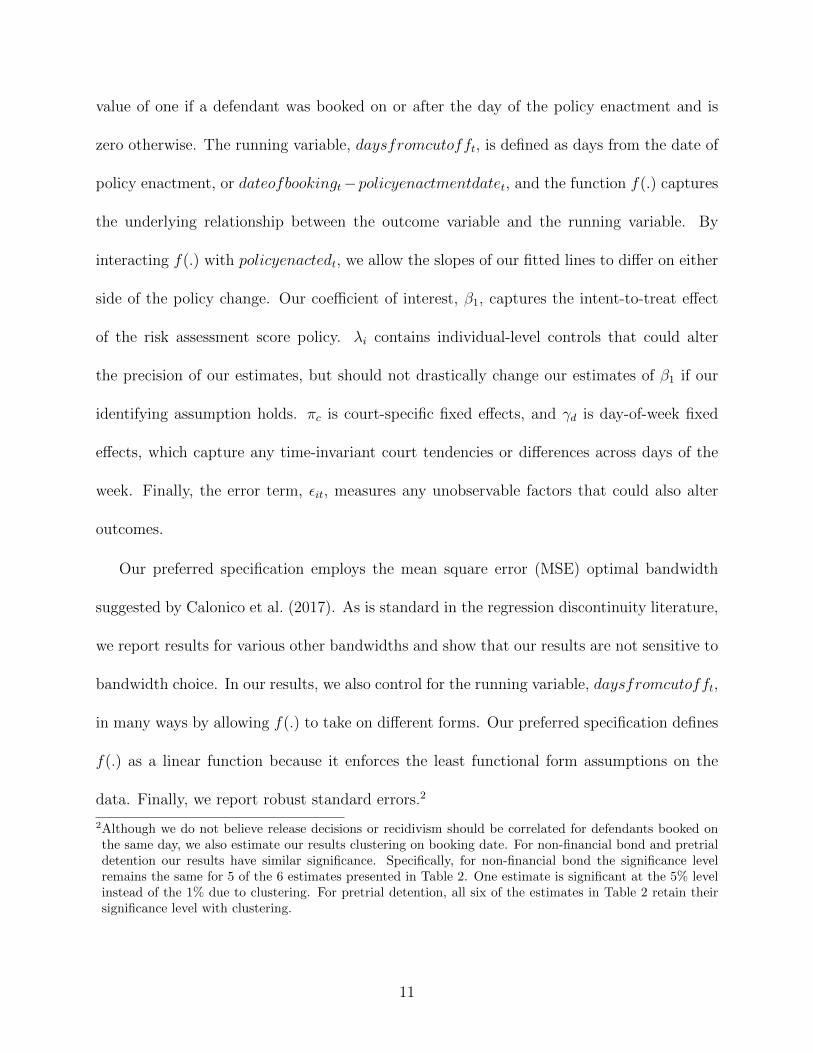
value of one if a defendant was booked on or after the day of the policy enactment and is

zero otherwise. The running variable, daysfromcutofft, is defined as days from the date of

policy enactment, or dateofbookingt−policyenactmentdatet, and the function f(.) captures

the underlying relationship between the outcome variable and the running variable. By

interacting f(.) with policyenactedt, we allow the slopes of our fitted lines to differ on either

side of the policy change. Our coefficient of interest, β1, captures the intent-to-treat effect

of the risk assessment score policy. λi contains individual-level controls that could alter

the precision of our estimates, but should not drastically change our estimates of β1 if our

identifying assumption holds. πc is court-specific fixed effects, and γd is day-of-week fixed

effects, which capture any time-invariant court tendencies or differences across days of the

week. Finally, the error term, εit, measures any unobservable factors that could also alter

outcomes.

Our preferred specification employs the mean square error (MSE) optimal bandwidth

suggested by Calonico et al. (2017). As is standard in the regression discontinuity literature,

we report results for various other bandwidths and show that our results are not sensitive to

bandwidth choice. In our results, we also control for the running variable, daysfromcutofft,

in many ways by allowing f(.) to take on different forms. Our preferred specification defines

f(.) as a linear function because it enforces the least functional form assumptions on the

data. Finally, we report robust standard errors.2

2Although we do not believe release decisions or recidivism should be correlated for defendants booked onthe same day, we also estimate our results clustering on booking date. For non-financial bond and pretrialdetention our results have similar significance. Specifically, for non-financial bond the significance levelremains the same for 5 of the 6 estimates presented in Table 2. One estimate is significant at the 5% levelinstead of the 1% due to clustering. For pretrial detention, all six of the estimates in Table 2 retain theirsignificance level with clustering.

11

4.2 Tests of Identification

Given the nature of the policy change noted before and the late implementation of the

policy (i.e., not on January 1), we believe it unlikely that defendants or judges could have

manipulated the assignment of treatment in a manner that would discredit our research

design. Even so, we provide empirical evidence that our identifying assumption is valid by

demonstrating that the number of defendants booked, as well as observable defendant and

case characteristics, do not vary discontinuously through the policy change threshold. Figure

1 shows the distribution of the running variable, days from the cutoff. If manipulation were

possible, we would expect to see a spike or fall in the number of defendants booked, but this

is not the case.

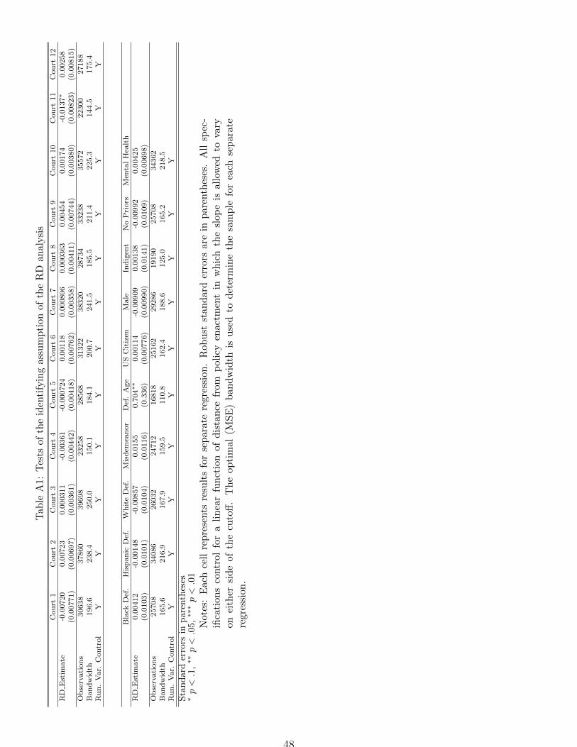
Next, we investigate if specific case and defendant characteristics are smooth through

the policy change threshold. If our identifying assumption is valid, defendant and case

characteristics will vary similarly on both sides of the policy change threshold. If defendants

or judges could have exactly manipulated the timing of booking, we would expect to find

differences in case and defendant characteristics through the policy enactment threshold. To

test this threat to identification, we estimate equation (1) using race, age, gender, criminal

history, indigent status, severity of arrest (misdemeanor or felony), mental health status, US

citizenship status, and specific court separately as outcome variables. Figure 2 and Appendix

Table 1 show the results for this test. There is only one small visible jump in defendant and

case characteristics in the graphs presented (Defendant Age). Of the 21 estimates presented

in Appendix Table 1, only two are statistically significant at conventional levels, although

with coefficients close to zero, which is consistent with findings due to chance. These results

12

indicate that case and defendant are not discontinuous through the policy change threshold.

We also present another test of the identifying assumption using all the covariates we

observe about a defendant and case that are determined before defendants are offered a

risk assessment score. Instead of considering the covariates individually, we use them in

combination along with a court and day-of-week fixed effect to predict the likelihood of

each potential outcome (release on non-financial bond, pretrial detention, non-violent and

violent recidivism) for every defendant. This allows us to create a weighted average where

the characteristics that contribute more to a specific outcome are considered with greater

weight. Here we can estimate the underlying probability that a defendant will be released

on non-financial bond, be detained pretrial, or recidviate using everything we know about

them except the use of a risk assessment score. If each predicted outcome is smooth through

the policy change threshold, then we can contribute any treatment effect we later estimate

to the policy change, not underlying differences in defendants booked just before and after

the policy change.

Figure 3 and Table A2 show the results for the predicted outcomes. The regression

discontinuity estimates for each predicted outcome are statistically insignificant and are

close to zero. This further indicates little evidence of underlying differences in defendants

across the policy change threshold—proving further that our identifying assumption holds.

13

5 Results

5.1 Effects of Risk Assessment Score Policy on Score Usage

To determine the effects of a risk assessment score policy, we first need to document that

Travis County’s enactment of its risk assessment score policy led to a sudden and dramatic

increase in the number of defendants assessed and assigned a risk assessment score. To do

so, we estimate equation (1) using the assignment of a risk assessment score as the outcome

variable. Figure 4 presents our graphical results. This graph and the graphs that follow

plot the mean of the outcome variable in 30-day bins and a linear fit of the outcome, which

is allowed to vary on each side of the policy change threshold. In all figures, the running

variable is normalized to zero (the date of policy enactment is zero days after the policy

change).

Figure 4 shows clearly that we estimate a large (about 80 percent) increase in risk as-

sessment score assignment across the policy change threshold.3 This indicates that about

80 percent of defendants booked after the policy enactment were assigned a risk assessment

score. We note that this is not a sharp discontinuity (i.e., 100 percent take-up), which mo-

tivates our use of intent-to-treat estimates used throughout the rest of the paper. There are

multiple reasons why a defendant may not have been recorded with a risk assessment score.

First, the Pretrial Services data we use are not perfect. It may be the case that some scores

simply were not recorded. Furthermore, some defendants are much less likely to receive a

risk assessment score, such as those who have an active defense attorney to convince Pretrial

3Risk assessment usage was greater than zero for a few months before January 2013 because Travis Countyelected to run a pilot study.

14

Services not to conduct a pretrial risk assessment score or those with a parole violation.

Regardless, our intent-to-treat effects allow us to estimate the unbiased intent-to-treat effect

of the risk assessment score policy.

5.2 Effects of a Risk Assessment Score Policy on Non-financial

Bond and Pretrial Release

The primary intent of the risk assessment adoption was to increase the number of defendants

released on non-financial bond. This decision is made by judges with access to risk assessment

scores, so this is the first outcome we consider. We also consider pretrial detention. If a

defendant is released on non-financial bond, they are not detained pretrial; but if a judge

offers financial bond to a defendant, their pretrial detention status is determined by their

ability to pay the bond. Therefore, it is of separate interest to determine the effects of a risk

assessment score on pretrial detention.

We first show the effects of risk assessment score on non-financial bonds and pretrial

detention in Figure 5. Formally, we estimate equation (1) with the probability of release on

non-financial bond and pretrial detention as outcome variables. Figure 5 shows the mean

of release on non-financial bond and pretrial detention in 30-day bins and a linear fit of the

outcome, which is allowed to vary on each side of the policy change threshold. This figure

provides visual evidence that implementing risk assessment scores increases the likelihood of

release on non-financial bond and decreases pretrial detention. It also appears these effects

fade with time. While it is challenging to determine exactly why our results decrease with

time, though we will discuss possible reasons later in this section.

15

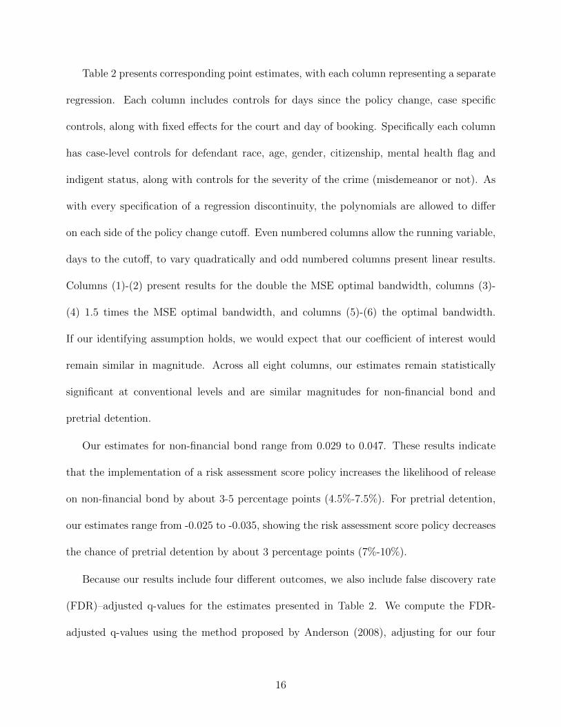
Table 2 presents corresponding point estimates, with each column representing a separate

regression. Each column includes controls for days since the policy change, case specific

controls, along with fixed effects for the court and day of booking. Specifically each column

has case-level controls for defendant race, age, gender, citizenship, mental health flag and

indigent status, along with controls for the severity of the crime (misdemeanor or not). As

with every specification of a regression discontinuity, the polynomials are allowed to differ

on each side of the policy change cutoff. Even numbered columns allow the running variable,

days to the cutoff, to vary quadratically and odd numbered columns present linear results.

Columns (1)-(2) present results for the double the MSE optimal bandwidth, columns (3)-

(4) 1.5 times the MSE optimal bandwidth, and columns (5)-(6) the optimal bandwidth.

If our identifying assumption holds, we would expect that our coefficient of interest would

remain similar in magnitude. Across all eight columns, our estimates remain statistically

significant at conventional levels and are similar magnitudes for non-financial bond and

pretrial detention.

Our estimates for non-financial bond range from 0.029 to 0.047. These results indicate

that the implementation of a risk assessment score policy increases the likelihood of release

on non-financial bond by about 3-5 percentage points (4.5%-7.5%). For pretrial detention,

our estimates range from -0.025 to -0.035, showing the risk assessment score policy decreases

the chance of pretrial detention by about 3 percentage points (7%-10%).

Because our results include four different outcomes, we also include false discovery rate

(FDR)–adjusted q-values for the estimates presented in Table 2. We compute the FDR-

adjusted q-values using the method proposed by Anderson (2008), adjusting for our four

16

different outcomes. The FDR q-values can be interpreted as adjusted p-values. The FDR

q-values for each outcome are statistically significant at least the five percent level for all but

one of the specifications. Therefore, we conclude that the effects we find are large enough

not to be attributed to chance.

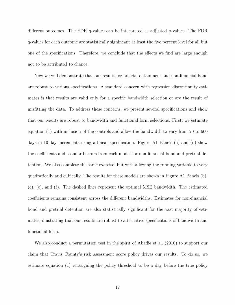
Now we will demonstrate that our results for pretrial detainment and non-financial bond

are robust to various specifications. A standard concern with regression discontinuity esti-

mates is that results are valid only for a specific bandwidth selection or are the result of

misfitting the data. To address these concerns, we present several specifications and show

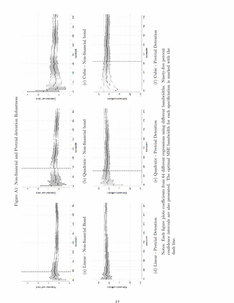
that our results are robust to bandwidth and functional form selections. First, we estimate

equation (1) with inclusion of the controls and allow the bandwidth to vary from 20 to 660

days in 10-day increments using a linear specification. Figure A1 Panels (a) and (d) show

the coefficients and standard errors from each model for non-financial bond and pretrial de-

tention. We also complete the same exercise, but with allowing the running variable to vary

quadratically and cubically. The results for these models are shown in Figure A1 Panels (b),

(c), (e), and (f). The dashed lines represent the optimal MSE bandwidth. The estimated

coefficients remains consistent across the different bandwidths. Estimates for non-financial

bond and pretrial detention are also statistically significant for the vast majority of esti-

mates, illustrating that our results are robust to alternative specifications of bandwidth and

functional form.

We also conduct a permutation test in the spirit of Abadie et al. (2010) to support our

claim that Travis County’s risk assessment score policy drives our results. To do so, we

estimate equation (1) reassigning the policy threshold to be a day before the true policy

17

change occurred. Because we only have data beginning in 2011, we are able to estimate

equation (1) 910 times using every possible date that occurred before the true policy change,

a linear specification, optimal bandwidth, and the controls included in Tables 2 and 3. The

distribution of placebo estimates for release on non-financial bond and pretrial detention is

shown in Figure A2. Nearly all placebo coefficients (97.99 percent) are less than the reported

estimates in Table 2 for release on non-financial bond. Our pretrial detention estimate in

Table 3 is less than 95.88 percent of our placebo estimates. These results provide further

evidence that our results are not simply due to chance.

Together these results show the adoption of a risk assessment scores policy caused in-

creased offers of non-financial bonds by judges which appears to lead to meaningful decreases

in pretrial detention. Since we find results for pretrial detention, we also consider if a risk

assessment score policy alters pretrial recidivism.

5.3 Effects of a Risk Assessment Score Policy on Recidivism

If it is the case that the new type of individuals released pretrial through non-financial bond

disproportionately commit crimes before their trial, there would be an increase in pretrial

recidivism. Results for non-violent and violent recidivism are shown in Figure 6. Both

graphs in Figure 6 show the mean of the outcome variable in 30-day bins and a linear fit of

the outcome, which is allowed to vary on each side of the policy change threshold. Figure

6 presents some suggestive evidence of a small increase in non-violent recidivism and no

change in non-violent recidivism. Table 3 presents the corresponding estimates. Similar

to Table 2, even columns allow the the running variable to vary quadratically and odd

18

columns are linear. Each column controls for defendant race, age, gender, citizenship, mental

health status, indigent status, and the severity of the crime (misdemeanor or not). Fixed

effects for the assigned court and booking day of the week are also included. Importantly,

our estimates for non-violent and violent estimates are of similar magnitudes across all six

columns. For non-violent recidivism, estimates range from 0.009 to 0.01 across the table.

Only three estimates are significant at the ten percent level. Although there appears to

be some evidence of small increases in non-violent recidivism, our results are not robust to

alternative specifications.

Next we consider violent recidivism. Across all columns our estimates remain stable,

ranging from -0.001 to -0.004. We are also able to rule out increases in violent recidivism

greater than 2 percent (.037 percentage points) when using the larger sample size from twice

the optimal bandwidth.4 We also report FDR q-values for recidivism outcomes. The FDR

q-values are also not consistently significant for either outcome.

We can also show our recidivism results are robust to alternative bandwidths and func-

tional forms. As we did for non-financial bond and pretrial detention, we estimate equation

(1) using non-violent and violent recidivism as outcomes, with the inclusion of the controls

and allow the bandwidth to vary from 20 to 660 days in 10-day increments. Figure A3 shows

the coefficients and standard errors from each model for non-violent and violent recidivism.

We also complete the same exercise, but with allowing the running variable to vary quadrat-

ically and cubically. The results for these models are shown in Figure A3 Panels (b), (c), (e),

and (f). The dashed lines represent the optimal MSE bandwidth. The estimated coefficients

remains consistent across the different bandwidths. Together these results indicate that risk

40.00037 is the top of the 95% confidence interval from this specification.

19

assessment scores do not increase violent-recidivism. We also find some evidence, although

not robust, of increases in nonviolent recidivism.

5.4 Indigent Defendants

Since one stated aim of the risk assessment score policy was to improve outcomes for low-

income defendants, we also present results for indigent versus non-indigent defendants. As

indigent defendants are more likely to be unable to post their bond before the policy change,

we would expect effects for release on non-financial bond and pretrial detention to be stronger

for indigent defendants compared to non-indigent defendants. Our graphical results are

shown in Figure 7. Entire sample results are replicated in Panel (a) and (d) for release on

non-financial bond and pretrial detention. Panels (b) and (e) present results for indigent

defendants, while Panels (c) and (f) show results for non-indigent defendants. For both

outcomes the discontinuity for indigent defendants is visibly larger than for non-indigent

defendants. There is also some evidence of an increase in release on non-financial bond and

a small decrease in pretrial detention for non-indigent defendants. Corresponding estimates

are shown in Table A3.

In Table A3, Panel A presents results for indigent defendants and Panel B show results for

non-indigent defendants. Similar to earlier result tables, each specification includes all case

controls. Even columns allow the running variable to vary quadratically and odd columns

are linear. Across each specification the coefficient for non-financial bond and pretrial de-

tention for indigent defendants has a greater magnitude, roughly two to three times larger,

than for non-indigent defendants, although we cannot rule out that the estimates are sta-

20

tistically equivalent. These subgroup results suggest that our release on non-financial bond

and pretrial detention results are likely driven by lower-income defendants.

We also explore results by indigent status for recidivism. As indigent defendants are the

most likely to be released pretrial it is possible that changes in their recidivism behavior are

masked in the entire sample results. Results for non-violent and violent recidivism are shown

in Figure 8. Panels (a) and (d) repeat the entire sample results for comparison. Indigent

results are show in Panels (b) and (e), while Panels (c) and (f) report results for non-

indigent defendants. For non-violent recidivism, there is some evidence of a larger increase

in recidivism for indigent defendants and no increase for non-indent defendants. For violent

recidivism however, there appears to be no increase in recidivism for indigent or non-indigent

defendants.

Table A4 shows recidivism estimates. For non-violent recidivism, the coefficients for

indigent defendants are larger in magnitude than for non-indigent defendants. For violent

recidivism, however, there are no meaningful differences in the coefficients for indigent and

non-indigent defendants. Further, for each subgroup the coefficient for violent recidivism is

negative, again suggesting there are no increases in violent recidivism across either group.

In summary, our results for indigent versus non-indigent defendants show that lower

income defendants are the most likely to be awarded non-financial bond and released pretrial.

We also find some suggestive evidence that non-violent recidivism may increase for lower

income defendants, who are most likely to be released. Violent recidivism does not increase

for either group.

21

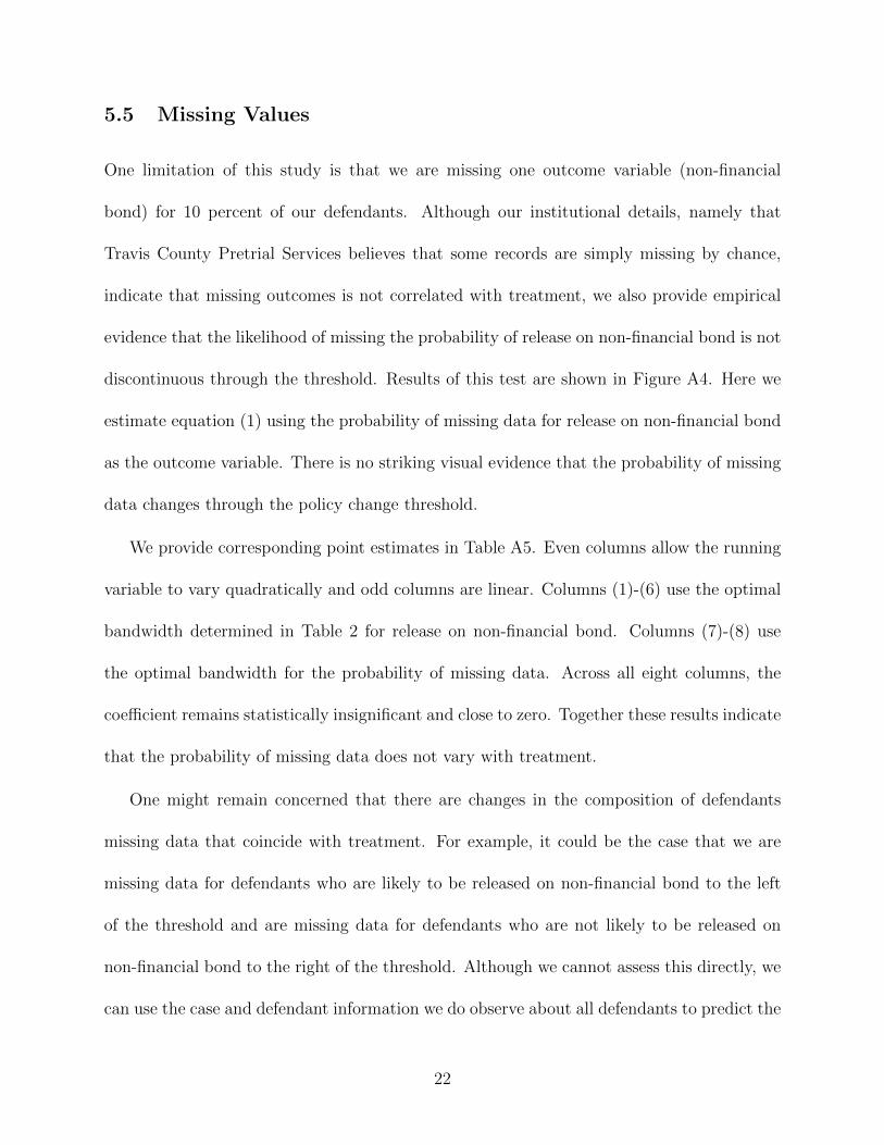
5.5 Missing Values

One limitation of this study is that we are missing one outcome variable (non-financial

bond) for 10 percent of our defendants. Although our institutional details, namely that

Travis County Pretrial Services believes that some records are simply missing by chance,

indicate that missing outcomes is not correlated with treatment, we also provide empirical

evidence that the likelihood of missing the probability of release on non-financial bond is not

discontinuous through the threshold. Results of this test are shown in Figure A4. Here we

estimate equation (1) using the probability of missing data for release on non-financial bond

as the outcome variable. There is no striking visual evidence that the probability of missing

data changes through the policy change threshold.

We provide corresponding point estimates in Table A5. Even columns allow the running

variable to vary quadratically and odd columns are linear. Columns (1)-(6) use the optimal

bandwidth determined in Table 2 for release on non-financial bond. Columns (7)-(8) use

the optimal bandwidth for the probability of missing data. Across all eight columns, the

coefficient remains statistically insignificant and close to zero. Together these results indicate

that the probability of missing data does not vary with treatment.

One might remain concerned that there are changes in the composition of defendants

missing data that coincide with treatment. For example, it could be the case that we are

missing data for defendants who are likely to be released on non-financial bond to the left

of the threshold and are missing data for defendants who are not likely to be released on

non-financial bond to the right of the threshold. Although we cannot assess this directly, we

can use the case and defendant information we do observe about all defendants to predict the

22

likelihood or release on non-financial bond for defendants who are missing this outcome. We

then estimate equation (1) using predicted probability of release on non-financial bond as

the outcome just for defendants who are missing data. Figure A5 shows these results. There

is no visual evidence of underlying differences in defendants who are missing data across the

threshold. Taken together, these results indicate that it is unlikely that the defendants with

outcomes missing from our dataset are sufficiently different to alter our results for release on

non-financial bond.

5.6 Long Term Effects

We now turn to why we only observe short-term effects that fade over time. Because our

regression discontinuity estimates only allow us to obtain local average treatment effects—or,

in other words, we can only establish the causal effects of the risk assessment score policy

just around the time of the policy change—we cannot credibly identify long-term effects of

the policy change. However, we can provide suggestive evidence on when the effects of the

policy begin to fade. To do so, we conduct event study analysis with results presented in

Figure A6.5 Visually, it is clear that the effect of non-financial bonds lasts for only two

months after the policy change and that the rate of release on non-financial bonds returns

to non-financial bond just afterward. It is natural to wonder why we see such a short-lived

effect from the risk assessment scores.

First, we note that Stevenson (2018b) also provided some evidence that the effects of

5Formally we regress probability of release on non-financial bond on indicators months before and after thepolicy change in two-month bins. Our regression also controls for race, age, gender, citizenship, mentalhealth status, and indigent status of the defendant, along with controls for the severity of the crime (mis-demeanor or not) and fixed effects for the assigned court and booking day of the week. Finally, we add acourt-specific time trend.

23

risk assessment scores fade with time, so this is not an uncommon pattern. Travis County

Pretrial Services also noted that judges and pretrial service employees did receive training

on the ORAS-PAT near its implementation, and that potential enthusiasm surrounding

the policy could have led to short term effects. For example, judges could have paid closer

attention to the scores right after the training, but stopped as time passed. It is also possible

that judges began to disregard the scores after the novelty of the policy change wore off.

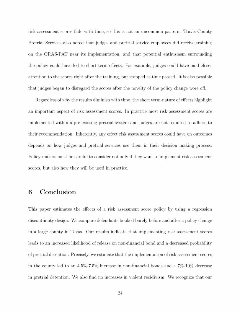
Regardless of why the results diminish with time, the short term-nature of effects highlight

an important aspect of risk assessment scores. In practice most risk assessment scores are

implemented within a pre-existing pretrial system and judges are not required to adhere to

their recommendation. Inherently, any effect risk assessment scores could have on outcomes

depends on how judges and pretrial services use them in their decision making process.

Policy-makers must be careful to consider not only if they want to implement risk assessment

scores, but also how they will be used in practice.

6 Conclusion

This paper estimates the effects of a risk assessment score policy by using a regression

discontinuity design. We compare defendants booked barely before and after a policy change

in a large county in Texas. Our results indicate that implementing risk assessment scores

leads to an increased likelihood of release on non-financial bond and a decreased probability

of pretrial detention. Precisely, we estimate that the implementation of risk assessment scores

in the county led to an 4.5%-7.5% increase in non-financial bonds and a 7%-10% decrease

in pretrial detention. We also find no increases in violent recidivism. We recognize that our

24

results are only for one county in Texas and that the extent to which they apply to other

contexts outside of Texas, where existing pretrial systems may be different, is unknown.

Further, it is possible that effects are only short-lived. Even with this qualification, we

believe that this study is an important contribution to nearly nonexistent literature on

risk assessment scores in practice. Our results indicate that risk assessment scores have

the potential to decrease costs to society and the disproportionate burden of financial bail

for low-income defendants, while not increasing violent pretrial recidivism. However, policy

makers must be careful to weigh these potential benefits with the potential for some increases

in non-violent recidivism.

25

References

Abadie, A., A. Diamond, and J. Hainmueller (2010). Synthetic control methods for compar-

ative case studies: Estimating the effect of california’s tobacco control program. Journal

of the American statistical Association 105 (490), 493–505.

Almond, L., M. McManus, D. Brian, and D. P. Merrington (2017). Exploration of the risk

factors contained within the uk’s existing domestic abuse risk assessment tool (dash): do

these risk factors have individual predictive validity regarding recidivism? Journal of

aggression, conflict and peace research 9 (1), 58–68.

Anderson, M. L. (2008). Multiple inference and gender differences in the effects of early inter-

vention: A reevaluation of the abecedarian, perry preschool, and early training projects.

Journal of the American statistical Association 103 (484), 1481–1495.

Bureau of Justice Statistics (2013, Dec). Felony defendants in large urban counties 2009

statistical tables. Bureau of Justice Statistics (BJS).

Calonico, S., M. D. Cattaneo, M. H. Farrell, and R. Titiunik (2017). rdrobust: Software for

regression discontinuity designs. Stata Journal 17 (2), 372–404.

Carmichael, D., G. Naufal, S. Wood, H. Caspers, and M. Marchbanks (2017). Liberty and

justice: Pretrial practices in texas.

Chanenson, S. L. and J. M. Hyatt (2016). The use of risk assessment at sentencing: Im-

plications for research and policy. Hyatt, JM & Chanenson, SL (2016). The Use of Risk

26

Assessment at Sentencing: Implications for Research and Policy. Bureau of Justice Assis-

tance, Washington, DC .

Craver, J. (2017, Mar). Travis county: No place for bondsmen. Austin Monitor .

DeMichele, M., P. Baumgartner, M. Wenger, K. Barrick, M. Comfort, and S. Misra (2018).

The public safety assessment: A re-validation and assessment of predictive utility and

differential prediction by race and gender in kentucky.

Didwania, S. H. (2018). The immediate consequences of pretrial detention: Evidence from

federal criminal cases.

Dobbie, W., J. Goldin, and C. S. Yang (2018). The Effects of Pretrial Detention on Convic-

tion, Future Crime, and Employment: Evidence from Randomly Assigned Judges. Amer-

ican Economic Review 108 (2), 201–40.

Dressel, J. and H. Farid (2018). The accuracy, fairness, and limits of predicting recidivism.

Science advances 4 (1), eaao5580.

Flores, A. W., A. M. Holsinger, C. T. Lowenkamp, and T. H. Cohen (2017). Time-free effects

in predicting recidivism using both fixed and variable follow-up periods: Do different

methods produce different results. Criminal justice and behavior 44 (1), 121–137.

Grove, W. M., D. H. Zald, B. S. Lebow, B. E. Snitz, and C. Nelson (2000). Clinical versus

mechanical prediction: a meta-analysis. Psychological assessment 12 (1), 19.

Gupta, A., C. Hansman, and E. Frenchman (2016). The heavy costs of high bail: Evidence

from judge randomization. The Journal of Legal Studies 45 (2), 471–505.

27

Heaton, P., S. Mayson, and M. Stevenson (2017). The downstream consequences of misde-

meanor pretrial detention. Stan. L. Rev. 69, 711.

Kleinberg, J., H. Lakkaraju, J. Leskovec, J. Ludwig, and S. Mullainathan (2017). Human

decisions and machine predictions. The quarterly journal of economics 133 (1).

Latessa, E. J., R. Lemke, M. Makarios, and P. Smith (2010). The creation and validation of

the ohio risk assessment system (oras). Fed. Probation 74, 16.

Leslie, E. and N. G. Pope (2016). The unintended impact of pretrial detention on case

outcomes: Evidence from nyc arraignments.(2016).

Meredith, T., J. C. Speir, and S. Johnson (2007). Developing and implementing automated

risk assessments in parole. Justice Research and Policy 9 (1), 1–24.

Schmidt, N., E. Lien, M. Vaughan, and M. T. Huss (2017). An examination of individual

differences and factor structure on the ls/cmi: does this popular risk assessment tool

measure up? Deviant behavior 38 (3), 306–317.

Smith, J. (2012, April). Keeping people in jail costs the county money, but is it in the best

interest of public safety? The Austin Chronicle.

Stevenson, M. (2018a). Distortion of justice: How the inability to pay bail affects case

outcomes. Journal of Law, Economics and Organization, Forthcoming .

Stevenson, M. T. (2018b). Assessing risk assessment in action. Minnesota Law Review

Forthcoming .

28

Travis County Criminal Courts (2012). Travis county criminal courts fair defense act pro-

gram.

Turner, S., J. Hess, and J. Jannetta (2009). Development of the california static risk assess-

ment instrument (csra). Center for Evidence-Based Corrections working paper, UC Irvine,

Irvine, CA.

United States Census Bureau (2017). U.s. census bureau quickfacts: Travis county. United

States Census Bureau.

United States Census Bureau (2018, July). County population totals and components of

change: 2010-2017. https://www.census.gov/data/datasets/2017/demo/popest/counties-

total.html.

Wagner, P. and B. Rabuy (2017, Jan). Following the money of mass incarceration.

Zhang, S. X., R. E. Roberts, and D. Farabee (2014). An analysis of prisoner reentry and

parole risk using compas and traditional criminal history measures. Crime & Delin-

quency 60 (2), 167–192.

29

Figures and Tables

Figure 1: Frequency of Running Variable

Notes: This figure shows the distribution of running variable observations near the adoption of riskassessment scores. Each bin is 2 days. The dashed line marks the day of the policy change.

30

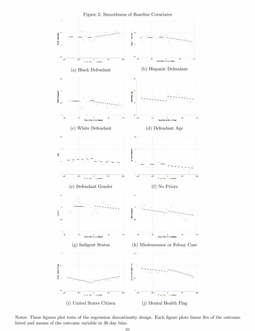
Figure 2: Smoothness of Baseline Covariates

(a) Black Defendant (b) Hispanic Defendant

(c) White Defendant (d) Defendant Age

(e) Defendant Gender (f) No Priors

(g) Indigent Status (h) Misdemeanor or Felony Case

(i) United States Citizen (j) Mental Health Flag

Notes: These figures plot tests of the regression discontinuity design. Each figure plots linear fits of the outcomelisted and means of the outcome variable in 30 day bins.

31

Figure 3: Regression Discontinuity Results for Predicted Values

(a) Predicted Probability of Release on Non-financial Bond (b) Predicted Probability Pretrial Detention

(c) Predicted Probability of Non-Violent Recidivism (d) Predicted Probability of Violent Recidivism

Notes: These figures plot tests of the regression discontinuity design. Each figure plots linear fits of the outcomelisted and means of the outcome variable in 30 day bins. Outcome variables are predicted using observable caseand defendant characteristics. Specifically we use race, age, gender, criminal history, indigent status, severity ofarrest, mental health status, US citizenship status, along with a court and day-of-week fixed effects. A bandwidthof 360 days is shown.

32

Figure 4: Regression Discontinuity Results for the Probability of Receiving a Risk Assessment Score

Notes: This figure shows the regression discountinuity estimate of the effect of implementing a risk assessmentscore policy on useage of risk assessment scores by ploting the mean of risk assessment score take-up in 30 daybins with linear fits. The outcome variable takes on a value of one if a defendant has a risk assemssment scoreand zero if she does not. A bandwidth of 360 days is shown.

33

Figure 5: Regression Discontinuity Results for Non-financial Bond and Pretrial Detention

(a) Non-financial Bond

(b) Pretrial Detention

Notes: This figure shows the regression discountinuity estimate of the effect of implementing a risk assessmentscore policy on the non-financial bond or pretrial detention by ploting the mean non-financial bond or pretrialdetention in 30 day bins with linear fits. A bandwidth of 360 days is shown.

34

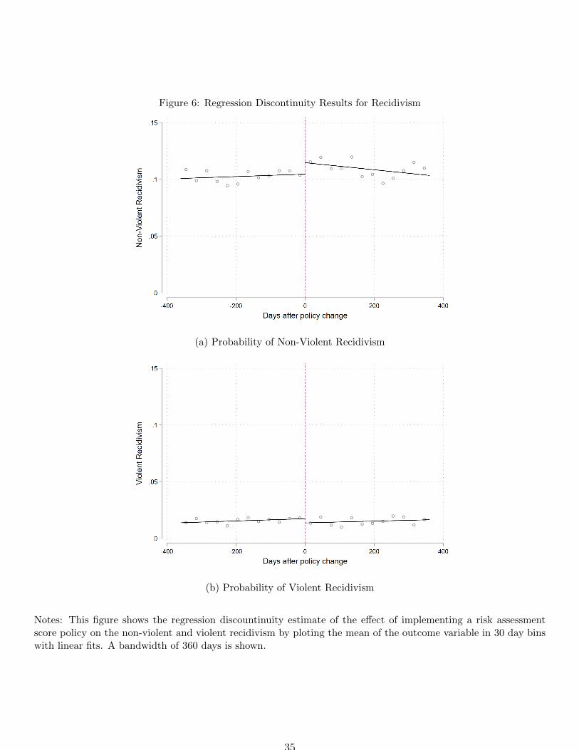
Figure 6: Regression Discontinuity Results for Recidivism

(a) Probability of Non-Violent Recidivism

(b) Probability of Violent Recidivism

Notes: This figure shows the regression discountinuity estimate of the effect of implementing a risk assessmentscore policy on the non-violent and violent recidivism by ploting the mean of the outcome variable in 30 day binswith linear fits. A bandwidth of 360 days is shown.

35

Fig

ure

7:In

dig

ent

Reg

ress

ion

Dis

conti

nu

ity

Res

ult

sfo

rN

on-fi

nan

cial

Bon

dand

Pre

tria

lD

eten

tion

(a)

Non

-fin

anci

alb

ond

-E

nti

reS

amp

le(b

)N

on-fi

nan

cial

bon

d-

Ind

igen

t(c

)N

on

-fin

an

cial

bon

d-

Non

-In

dig

ent

(d)

Pre

tria

lD

eten

tion

-E

nti

reS

amp

le(e

)P

retr

ial

Det

enti

on-

Ind

igen

t(f

)P

retr

ial

Det

enti

on

-N

on

-In

dig

ent

Not

es:

Th

isfi

gure

show

sth

ere

gres

sion

dis

cou

nti

nu

ity

esti

mat

eof

the

effec

tof

imp

lem

enti

ng

ari

skass

essm

ent

scor

ep

olic

yon

the

non

-fin

anci

alb

ond

orp

retr

ial

det

enti

onby

plo

ting

the

mea

nn

on

-fin

an

cial

bon

dor

pre

tria

ld

eten

tion

in30

day

bin

sw

ith

lin

ear

fits

.A

ban

dw

idth

of36

0d

ays

issh

own

.

36

Fig

ure

8:In

dig

ent

Reg

ress

ion

Dis

conti

nu

ity

Res

ult

sfo

rR

ecid

ivis

m

(a)

Non

-vio

lent

Rec

idiv

ism

-E

nti

reS

amp

le(b

)N

on-v

iole

nt

Rec

idiv

ism

-In

dig

ent

(c)

Non

-vio

lent

Rec

idiv

ism

-N

on

-In

dig

ent

(d)

Vio

lent

Rec

idiv

ism

-E

nti

reS

amp

le(e

)V

iole

nt

Rec

idiv

ism

-In

dig

ent

(f)

Vio

lent

Rec

idiv

ism

-N

on

-In

dig

ent

Not

es:

Th

isfi

gure

show

sth

ere

gres

sion

dis

cou

nti

nu

ity

esti

mat

eof

the

effec

tof

imp

lem

enti

ng

ari

skass

essm

ent

scor

ep

olic

yon

the

non

-fin

anci

alb

ond

orp

retr

ial

det

enti

onby

plo

ting

the

mea

nn

on

-fin

an

cial

bon

dor

pre

tria

ld

eten

tion

in30

day

bin

sw

ith

lin

ear

fits

.A

ban

dw

idth

of36

0d

ays

issh

own

.

37

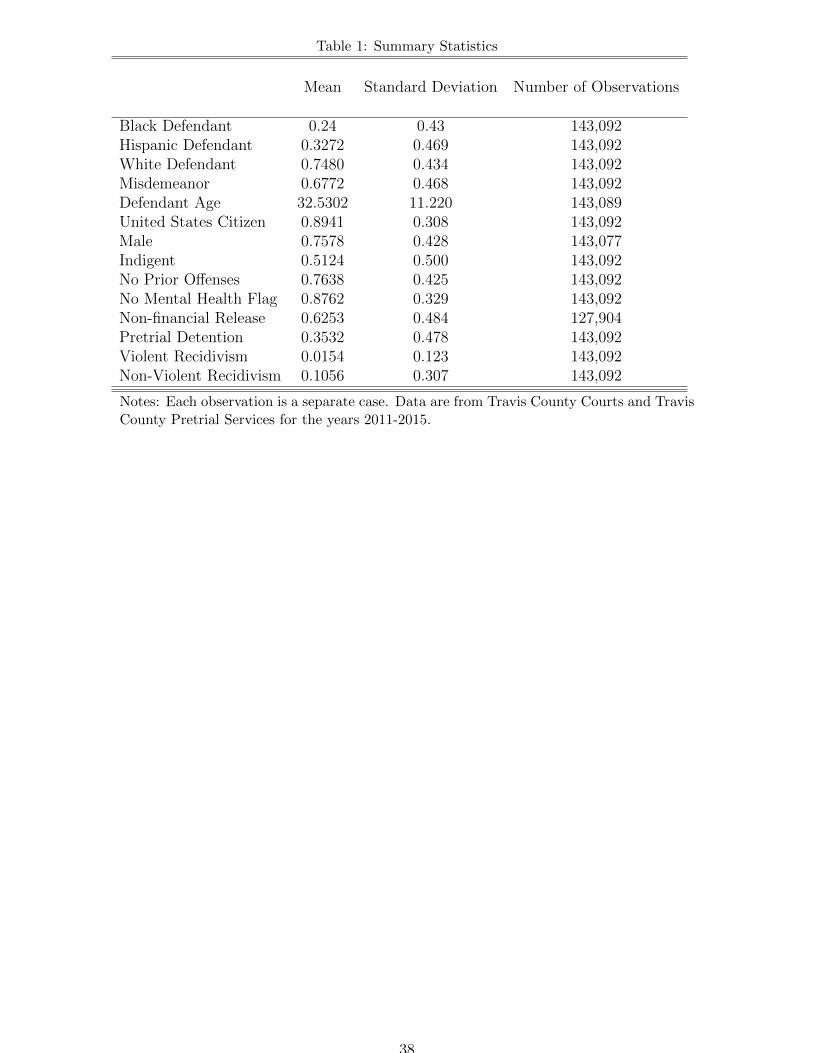
Table 1: Summary Statistics

Mean Standard Deviation Number of Observations

Black Defendant 0.24 0.43 143,092Hispanic Defendant 0.3272 0.469 143,092White Defendant 0.7480 0.434 143,092Misdemeanor 0.6772 0.468 143,092Defendant Age 32.5302 11.220 143,089United States Citizen 0.8941 0.308 143,092Male 0.7578 0.428 143,077Indigent 0.5124 0.500 143,092No Prior Offenses 0.7638 0.425 143,092No Mental Health Flag 0.8762 0.329 143,092Non-financial Release 0.6253 0.484 127,904Pretrial Detention 0.3532 0.478 143,092Violent Recidivism 0.0154 0.123 143,092Non-Violent Recidivism 0.1056 0.307 143,092

Notes: Each observation is a separate case. Data are from Travis County Courts and TravisCounty Pretrial Services for the years 2011-2015.

38

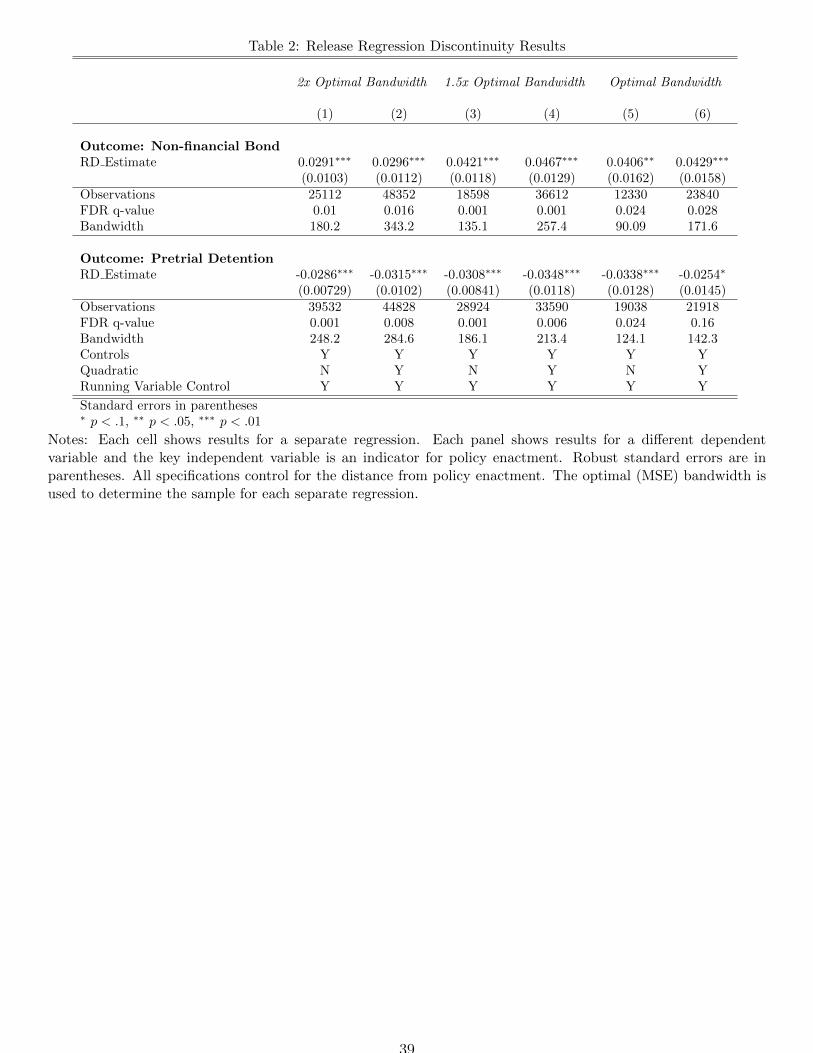
Table 2: Release Regression Discontinuity Results

2x Optimal Bandwidth 1.5x Optimal Bandwidth Optimal Bandwidth

(1) (2) (3) (4) (5) (6)

Outcome: Non-financial BondRD Estimate 0.0291∗∗∗ 0.0296∗∗∗ 0.0421∗∗∗ 0.0467∗∗∗ 0.0406∗∗ 0.0429∗∗∗

(0.0103) (0.0112) (0.0118) (0.0129) (0.0162) (0.0158)Observations 25112 48352 18598 36612 12330 23840FDR q-value 0.01 0.016 0.001 0.001 0.024 0.028Bandwidth 180.2 343.2 135.1 257.4 90.09 171.6

Outcome: Pretrial DetentionRD Estimate -0.0286∗∗∗ -0.0315∗∗∗ -0.0308∗∗∗ -0.0348∗∗∗ -0.0338∗∗∗ -0.0254∗

(0.00729) (0.0102) (0.00841) (0.0118) (0.0128) (0.0145)Observations 39532 44828 28924 33590 19038 21918FDR q-value 0.001 0.008 0.001 0.006 0.024 0.16Bandwidth 248.2 284.6 186.1 213.4 124.1 142.3Controls Y Y Y Y Y YQuadratic N Y N Y N YRunning Variable Control Y Y Y Y Y Y

Standard errors in parentheses∗ p < .1, ∗∗ p < .05, ∗∗∗ p < .01

Notes: Each cell shows results for a separate regression. Each panel shows results for a different dependentvariable and the key independent variable is an indicator for policy enactment. Robust standard errors are inparentheses. All specifications control for the distance from policy enactment. The optimal (MSE) bandwidth isused to determine the sample for each separate regression.

39

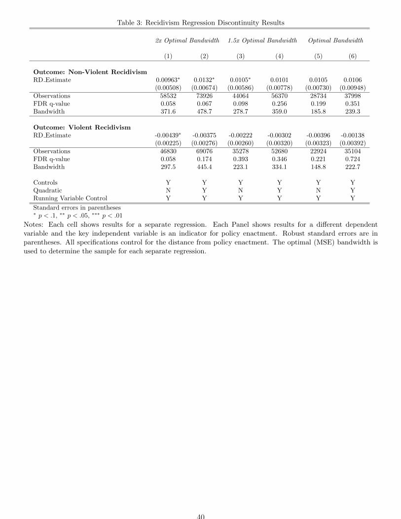
Table 3: Recidivism Regression Discontinuity Results


(1) (2) (3) (4) (5) (6)

Outcome: Non-Violent RecidivismRD Estimate 0.00963∗ 0.0132∗ 0.0105∗ 0.0101 0.0105 0.0106


Outcome: Violent RecidivismRD Estimate -0.00439∗ -0.00375 -0.00222 -0.00302 -0.00396 -0.00138


Controls Y Y Y Y Y YQuadratic N Y N Y N YRunning Variable Control Y Y Y Y Y Y


Notes: Each cell shows results for a separate regression. Each Panel shows results for a different dependentvariable and the key independent variable is an indicator for policy enactment. Robust standard errors are inparentheses. All specifications control for the distance from policy enactment. The optimal (MSE) bandwidth isused to determine the sample for each separate regression.

40

A Appendix

41

Fig

ure

A1:

Non

-fin

anci

alan

dP

retr

ial

det

enti

onR

ob

ust

nes

s

(a)

Lin

ear

-N

on-fi

nan

cial

Bon

d(b

)Q

uad

rati

c-

Non

-fin

anci

alb

ond

(c)

Cu

bic

-N

on

-fin

an

cial

bon

d

(d)

Lin

ear

-P

retr

ial

Det

enti

on(e

)Q

uad

rati

c-

Pre

tria

lD

eten

tion

(f)

Cu

bic

-P

retr

ial

Det

enti

on

Not

es:

Eac

hfi

gure

plo

tsco

effici

ents

from

64d

iffer

ent

regr

essi

ons

usi

ng

diff

eren

tb

an

dw

idth

s.N

inet

y-fi

ve

per

cent

con

fid

ence

inte

rval

sar

eal

sop

rese

nte

d.

Th

eop

tim

alM

SE

ban

dw

idth

for

each

spec

ifici

ati

on

ism

ark

edw

ith

the

das

hli

ne.

42

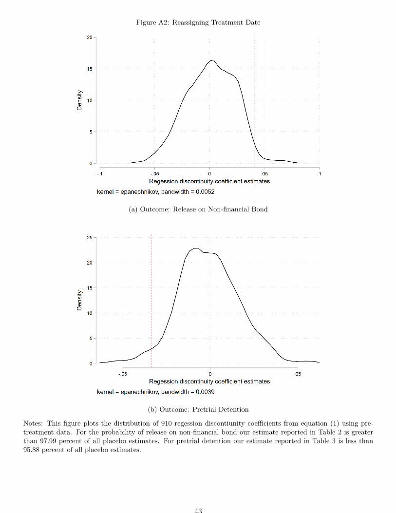
Figure A2: Reassigning Treatment Date

(a) Outcome: Release on Non-financial Bond

(b) Outcome: Pretrial Detention

Notes: This figure plots the distribution of 910 regession discontiunity coefficients from equation (1) using pre-treatment data. For the probability of release on non-financial bond our estimate reported in Table 2 is greaterthan 97.99 percent of all placebo estimates. For pretrial detention our estimate reported in Table 3 is less than95.88 percent of all placebo estimates.

43

Fig

ure

A3:

Rec

idiv

ism

Rob

ust

nes

s

(a)

Lin

ear

-V

iole

nt

Rec

idiv

ism

(b)

Qu

adra

tic

-V

iole

nt

Rec

idiv

ism

(c)

Cu

bic

-V

iole

nt

Rec

idiv

ism

(d)

Lin

ear

-N

on-V

iole

nt

Rec

idiv

ism

(e)

Qu

adra

tic

-N

on-V

iole

nt

Rec

idiv

ism

(f)

Cu

bic

-N

on

-Vio

lent

Rec

idiv

ism

Not

es:

Eac

hfi

gure

plo

tsco

effici

ents

from

64d

iffer

ent

regr

essi

ons

usi

ng

diff

eren

tb

an

dw

idth

s.N

inet

y-fi

ve

per

cent

con

fid

ence

inte

rval

sar

eal

sop

rese

nte

d.

Th

eop

tim

alM

SE

ban

dw

idth

for

each

spec

ifici

ati

on

ism

ark

edw

ith

the

das

hli

ne.

44

Figure A4: Regression Discontinuity Results for Probability of Missing Outcome Data

Notes: This figure shows the regression discountinuity estimate of the effect of implementing a risk assessmentscore policy on the likelihood of missing data on probability of release on non-financial bond by ploting the meanof the probability of missing in 30 day bins with linear fits. A bandwidth of 360 days is shown.

45

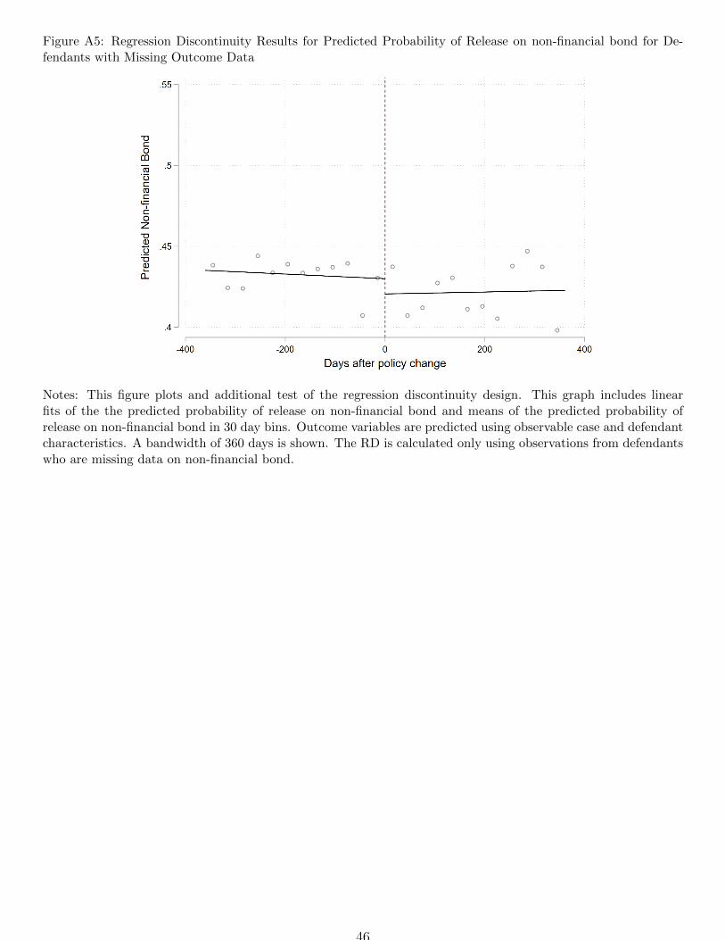
Figure A5: Regression Discontinuity Results for Predicted Probability of Release on non-financial bond for De-fendants with Missing Outcome Data

Notes: This figure plots and additional test of the regression discontinuity design. This graph includes linearfits of the the predicted probability of release on non-financial bond and means of the predicted probability ofrelease on non-financial bond in 30 day bins. Outcome variables are predicted using observable case and defendantcharacteristics. A bandwidth of 360 days is shown. The RD is calculated only using observations from defendantswho are missing data on non-financial bond.

46

Figure A6: Dynamic Effects of Risk Assessment Scores

Notes: This figure plots the coefficients from the regression of non-financial bond on indicators for months beforeor after risk assessment adoption. Individual level controls for race, age, gender, citizenship and indigent statusof the defendant along with controls for the severity of the crime (misdemeanor or not) as well as fixed effects forthe court assigned and day-of-week of booking. A court-specific time trend is also included.

47

Tab

leA

1:T

ests

ofth

eid

enti

fyin

gas

sum

pti

onof

the

RD

an

aly

sis

Court

1Court

2Court

3Court

4Court

5Court

6Court

7Court

8Court

9Court

10

Court

11

Court

12

RD

Estim

ate

-0.00720

0.00723

0.000311

-0.00361

-0.000724

0.00118

0.000806

0.000363

0.00454

0.00174

-0.0137∗

0.00258

(0.00771)

(0.00697)

(0.00361)

(0.00442)

(0.00418)

(0.00762)

(0.00358)

(0.00411)

(0.00744)

(0.00380)

(0.00823)

(0.00815)

Observations

30638

37860

39698

23258

28568

31322

38320

28734

33238

35572

22300

27188

Bandwidth

196.6

238.4

250.0

150.1

184.1

200.7

241.5

185.5

211.4

225.3

144.5

175.4

Run.Var.

Control

YY

YY

YY

YY

YY

YY

Black

Def.

Hispanic

Def.

WhiteDef.

Misdem

eanor

Def.Age

USCitizen

Male

Indigen

tNoPriors

Men

talHea

lth

RD

Estim

ate

0.00412

-0.00148

-0.00857

0.0155

0.704∗∗

0.00114

-0.00909

0.00138

-0.00992

0.00425

(0.0103)

(0.0101)

(0.0104)

(0.0116)

(0.336)

(0.00776)

(0.00990)

(0.0141)

(0.0109)

(0.00698)

Observations

25708

34086

26032

24712

16818

25162

29286

19190

25708

34362

Bandwidth

165.6

216.9

167.9

159.5

110.8

162.4

188.6

125.0

165.2

218.5

Run.Var.

Control

YY

YY

YY

YY

YY

Sta

nd

ard

erro

rsin

par

enth

eses

∗p<

.1,∗∗

p<

.05,

∗∗∗p<

.01

Not

es:

Eac

hce

llre

pre

sents

resu

lts

for

sep

arat

ere

gres

sion

.R

obu

stst

and

ard

erro

rsare

inp

are

nth

eses

.A

llsp

ec-

ifica

tion

sco

ntr

olfo

ra

lin

ear

fun

ctio

nof

dis

tan

cefr

omp

olic

yen

actm

ent

inw

hic

hth

esl

op

eis

all

owed

tova

ryon

eith

ersi

de

ofth

ecu

toff

.T

he

opti

mal

(MS

E)

ban

dw

idth

isu

sed

todet

erm

ine

the

sam

ple

for

each

sep

ara

tere

gres

sion

.

48

Table A2: Regression Discontinuity Results for Predicted Outcomes

Optimal Bandwidth

(1) (2)

Outcome: Predicted Non-financial BailRD Estimate 0.000200 0.000128

(0.00800) (0.00872)Observations 13744 26600Bandwidth 90.09 171.6

Outcome: Predicted Non-Violent RecidivismRD Estimate -0.00501 0.00526


Outcome: Predicted Non-Violent RecidivismRD Estimate 0.00212 0.000900


Outcome: Predicted Violent RecidivismRD Estimate -0.000994 -0.00126


Controls N NQuadratic N YRunning Variable Control Y Y


Notes: Each cell represents results for a separate regression where the key independent variable is an indicatorof policy enactment. Robust standard errors are in parentheses. All specifications control for the distance frompolicy enactment. The optimal (MSE) bandwidth from Table 2 and Table 3 (the optimal bandwidth for the actualoutcome variable) is used to determine the sample for each separate regression. Outcome variables are predictedusing observable case and defendant characteristics. Specifically we use race, age, gender, criminal history, indigentstatus, severity of arrest, mental health status, US citizenship status, along with a court and day-of-week fixedeffect. Column (1) presents a linear functinal form and column (2) is quadratic.

49

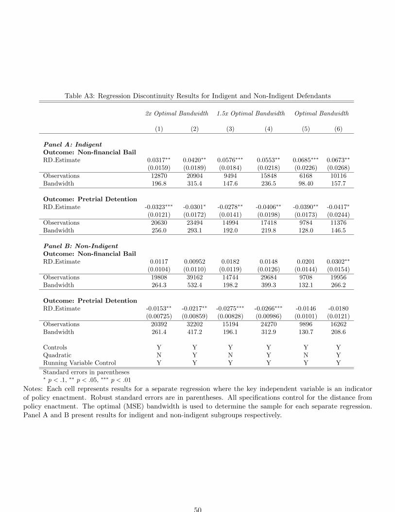
Table A3: Regression Discontinuity Results for Indigent and Non-Indigent Defendants


(1) (2) (3) (4) (5) (6)

Panel A: IndigentOutcome: Non-financial BailRD Estimate 0.0317∗∗ 0.0420∗∗ 0.0576∗∗∗ 0.0553∗∗ 0.0685∗∗∗ 0.0673∗∗

(0.0159) (0.0189) (0.0184) (0.0218) (0.0226) (0.0268)Observations 12870 20904 9494 15848 6168 10116Bandwidth 196.8 315.4 147.6 236.5 98.40 157.7

Outcome: Pretrial DetentionRD Estimate -0.0323∗∗∗ -0.0301∗ -0.0278∗∗ -0.0406∗∗ -0.0390∗∗ -0.0417∗


Panel B: Non-IndigentOutcome: Non-financial BailRD Estimate 0.0117 0.00952 0.0182 0.0148 0.0201 0.0302∗∗


Outcome: Pretrial DetentionRD Estimate -0.0153∗∗ -0.0217∗∗ -0.0275∗∗∗ -0.0266∗∗∗ -0.0146 -0.0180




Notes: Each cell represents results for a separate regression where the key independent variable is an indicatorof policy enactment. Robust standard errors are in parentheses. All specifications control for the distance frompolicy enactment. The optimal (MSE) bandwidth is used to determine the sample for each separate regression.Panel A and B present results for indigent and non-indigent subgroups respectively.

50

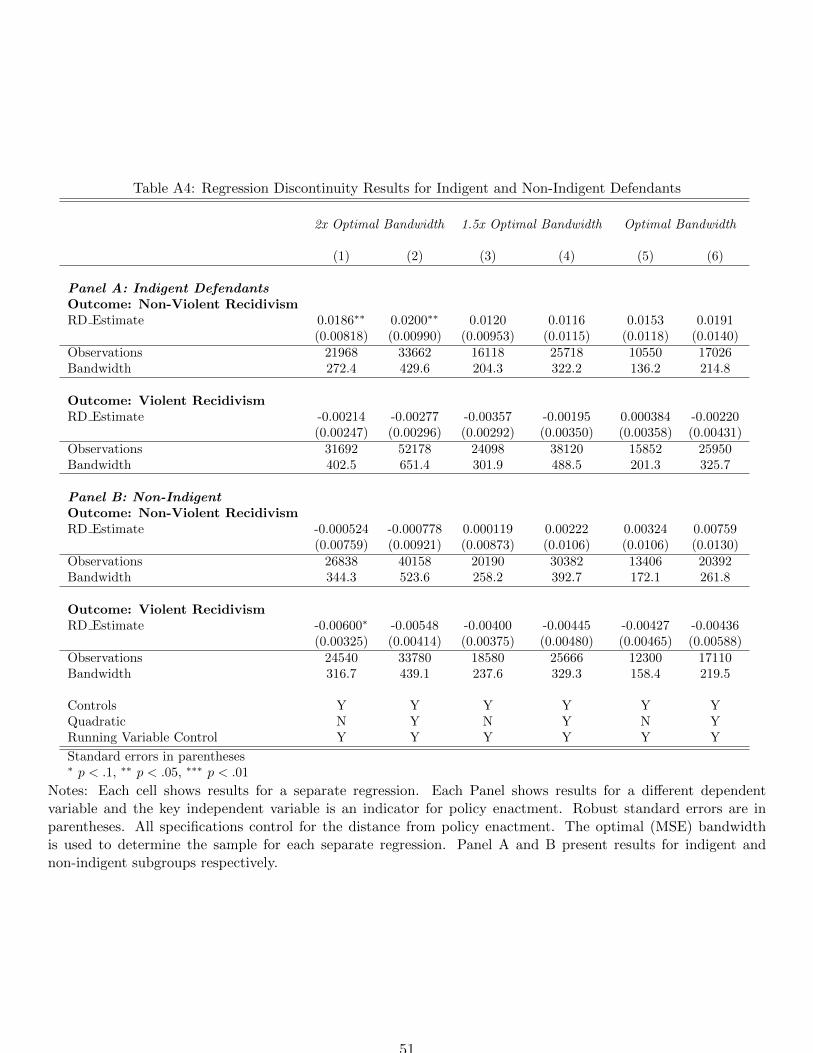
Table A4: Regression Discontinuity Results for Indigent and Non-Indigent Defendants


(1) (2) (3) (4) (5) (6)

Panel A: Indigent DefendantsOutcome: Non-Violent RecidivismRD Estimate 0.0186∗∗ 0.0200∗∗ 0.0120 0.0116 0.0153 0.0191


Outcome: Violent RecidivismRD Estimate -0.00214 -0.00277 -0.00357 -0.00195 0.000384 -0.00220


Panel B: Non-IndigentOutcome: Non-Violent RecidivismRD Estimate -0.000524 -0.000778 0.000119 0.00222 0.00324 0.00759


Outcome: Violent RecidivismRD Estimate -0.00600∗ -0.00548 -0.00400 -0.00445 -0.00427 -0.00436




Notes: Each cell shows results for a separate regression. Each Panel shows results for a different dependentvariable and the key independent variable is an indicator for policy enactment. Robust standard errors are inparentheses. All specifications control for the distance from policy enactment. The optimal (MSE) bandwidthis used to determine the sample for each separate regression. Panel A and B present results for indigent andnon-indigent subgroups respectively.

51

Tab

leA

5:R

egre

ssio

nD

isco

nti

nu

ity

Res

ult

sfo

rth

eP

rob

ab

ilit

yof

Mis

sin

gD

ata

2xO

ptim

alB

andw

idth

1.5x

Opt

imal

Ban

dwid

thO

ptim

alB

andw

idth

Opt

imal

Ban

dwid

thfo

rP

r(M

issi

ng)

Outc

om

e:

Mis

sing

Data

(1)

(2)

(3)

(4)

(5)

(6)

(7)

(8)

RD

Est

imat

e-0

.005

270.

0008

07-0

.006

59-0

.005

990.

0000

473

-0.0

0623

-0.0

0635

0.00

380

(0.0

0527

)(0

.008

43)

(0.0

0620

)(0

.006

75)

(0.0

0712

)(0

.007

78)

(0.0

0966

)(0

.009

46)

Obse

rvat

ions

4060

034

086

2801

654

084

2077

840

934

1374

426

600

Ban

dw

idth

255.

321

6.8

180.

234

3.2

135.

125

7.4

90.0

917

1.6

Con

trol

sY

YY

YY

YY

YQ

uad

rati

cN

YN

YN

YN

YR

un.

Var

.C

ontr

olY

YY

YY

YY

Y

Sta

nd

ard

erro

rsin

par

enth

eses

∗p<

.1,∗∗

p<

.05,

∗∗∗p<

.01

Not

es:

Eac

hce

llre

pre

sents

resu

lts

for

sep

arat

ere

gres

sion

.E

ach

colu

mn

pre

sents

resu

lts

for

the

pro

bab

ilit

yof

mis

sin

gd

ata

for

the

outc

ome

vari

able

pro

babi

lity

of

non

-fin

an

cial

rele

ase

an

dth

eke

yin

dep

end

ent

vari

ab

leis

an

ind

icat

orfo

rp

olic

yen

actm

ent.

Rob

ust

stan

dar

der

rors

are

inp

aren

thes

es.

All

spec

ifica

tion

sco

ntr

ol

for

ali

nea

rfu

nct

ion

ofd

ista

nce

from

pol

icy

enac

tmen

tin

wh

ich

the

slop

eis

allo

wed

tova

ryon

eith

ersi

de

of

the

cuto

ff.

Th

eop

tim

al(M

SE

)b

and

wid

this

use

dto

det

erm

ine

the

sam

ple

for

each

sep

arate

regre

ssio

nin

the

firs

tth

ree

colu

mn

s.C

olu

mn

s(1

)-(6

)u

seth

eop

tim

alb

and

wid

thd

eter

min

edin

Tab

le2.

Col

um

ns

(7)-

(8)

use

the

op

tim

al

band

wid

thfo

rth

eP

rob

abil

ity

ofM

issi

ng

Dat

a.

52

diion paper erieftp.iza.org/dp11948.pdfdiion paper erie iza dp no. 11948 carlywill sloan george...

Documents