digital speech processing— lecture 10 short-time fourier
TRANSCRIPT
1
Digital Speech Processing—Lecture 10
Short-Time Fourier Analysis Methods - Filter
Bank Design
2
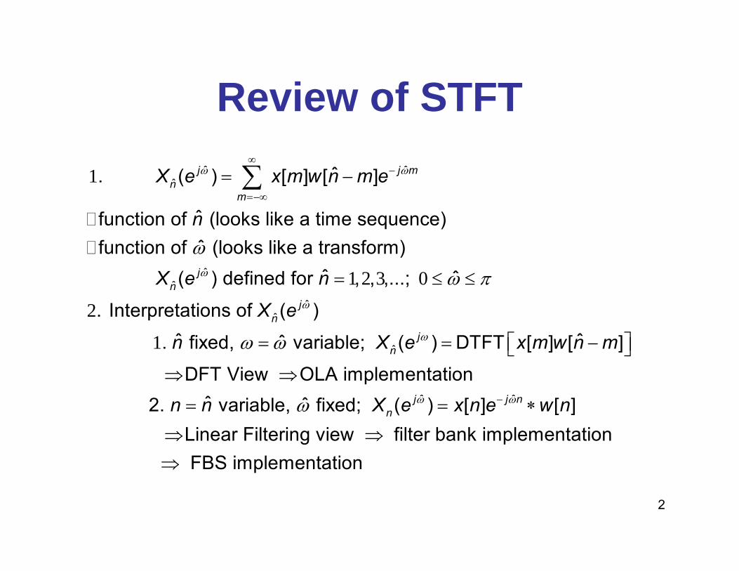
Review of STFT1
1 2 3 0
2
1
ˆ ˆˆ
ˆˆ
ˆˆ
ˆ. ( ) [ ] [ ]
ˆ function of (looks like a time sequence)ˆ function of (looks like a transform)
ˆ ˆ( ) defined for , , ,...;
. Interpretations of ( )ˆ. fix
ω ω
ω
ω
ω
ω π
∞−
=−∞
= −
= ≤ ≤
∑j j mn
m
jn
jn
X e x m w n m e
n
X e n
X e
n ˆ
ˆ ˆ
ˆˆed, variable; ( ) DTFT [ ] [ ]
DFT View OLA implementationˆ ˆ 2. variable, fixed; ( ) [ ] [ ]
Linear Filtering view filter bank implementation FBS i
ω
ω ω
ω ω
ω −
= = −⎡ ⎤⎣ ⎦⇒ ⇒
= = ∗
⇒ ⇒⇒
jn
j j nn
X e x m w n m
n n X e x n e w n
mplementation
3
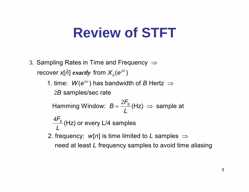
Review of STFT
3
22
ˆˆ
. Sampling Rates in Time and Frequency ˆrecover [ ] from ( )
1. time: ( ) has bandwidth of Hertz samples/sec rate
Hamming Window: (Hz) sample
ω
ω
⇒
⇒
= ⇒
jn
j
S
x n X e
W e BB
FBL
exactly
4
at
(Hz) or every L/4 samples
2. frequency: [ ] is time limited to samples need at least frequency samples to avoid time aliasing
⇒
SFL
w n LL

4
Review of STFT with OLA method can recover ( ) using lower
sampling rates in either time or frequency, e.g., can sample every samples (and divide by window), or can use fewer than frequency sam
x n
LL
exactly
ples (filter bank channels); but these methods are highly subject to aliasing errors with any modifications to STFT can use windows (LPF) that are longer than samples and
still recover with L
frequency channels; e.g., ideal LPF is infinite in time duration, but with zeros spaced samples apart where / is the BW of the ideal LPF
< ⇒
S
N LN
F N

5
Review of STFTH0(ejω)
H1(ejω)
HN-1(ejω)
+…
X(ejω) Y(ejω)
1
0
1
0
1
0
[ ] [ ]
( ) ( )
[ ] [ ] [ ] [ ] [ ]
[ ] [ ]
[ ] [ ] [ ] [ ] [ ] ...
need to design digital filters that match criteria for exact reconstr
ω
ω ω
δ
δ
δ
−
=
−
=
∞
=−∞
∞
=−∞
=
= =
= = =
= −
= − = + +
⇒
∑
∑
∑
∑
%
%
%
kj nk
Nj j
kk
N
kk
r
r
h n w n e
H e H e
h n h n n w n p n
p n N n rN
h n N w rN n rN w w N
uction of [ ] and which still work with modifications to STFTx n

Tree-Decimated Filter Banks
6

Tree-Decimated Filter Banks• can sample STFT in time and frequency using lowpass
filter (window) which is moved in jumps of R<L samples if L≤N where:– L is the window length, – R is the window shift, and – N is the number of frequency channels
• for a given channel at ω=ωk, the sampling rate of the STFT need only be twice the bandwidth of the window Fourier transform– down-sample STFT estimates by a factor of R at the transmitter– up-sample back to original sampling rate at the receiver– final output formed by convolution of the up-sampled STFT with
an appropriate lowpass filter, f [n]7

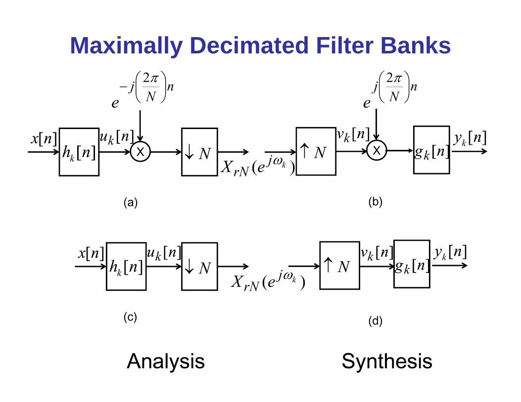
Filter Bank Channels
8
Fully decimated and interpolated filter bank channels; (a) analysis with bandpass filter, down-shifting frequency and down-sampling; (b) synthesis with up-sampler followed by lowpassinterpolation filter and frequency up-shift; (c) analysis with frequency down-shift followed by lowpass filter followed by down-sampling; (d) synthesis with up-sampling followed by frequency up-shift followed by bandpass filter.

Full Implementation of Analysis-Synthesis System
9
Full implementation of STFT analysis/synthesis system with channel decimation by a factor of R, and channel interpolation by the same factor R (including a box for short-time modifications.

10
Review of Down and Up-Sampling
R↓][nx [ ] [ ]dx n x nR=
11 2
0
( )/( ) ( )
aliasing addition
ω ω π−
−
=
= ∑R
j j r Rd R
rX e X e
R↑][nx[ / ] 0, 1, 2,...
[ ]0 otherwiseu
x n R nx n
= ± ±⎧= ⎨⎩
( ) ( ) imaging removal
ω ω=j j RuX e X e

11
[ ]
1
0
1
0
1
1
1 ( )
assuming no short time modifications ( ) ( ) ( ) ( )
( ) ( ) ( )
( ) [ ] [ ]
( ) ( ) ( ) ( )
k k
rR
k k
k
k
rR
j j mrR rR
m W
Nj j n
rRkN
j nrR
k
j n m
m W r k
X k X e w rR m x m e
y n P k Y e eN
P k X k f n rR eN
x m w rR m f n rR P k eN
ω ω
ω ω
ω
ω
−
∈
−
=
−
=
∞−
∈ =−∞ =
•
= = −
=
= −
⎡ ⎤= − −⎢ ⎥
⎣ ⎦
∑
∑
∑
∑ ∑1
0
1
0
11 ( )
recognizing that when ( ) ,
( )
can show that the condition for ( ) ( ), is
( ) ( ) ( )
k
N
Nj n m
k q
r
P k k
e n m qNN
y n x n n
w rR n qN f n rR q m n
ω δ
δ
−
− ∞−
= =−∞
∞
=−∞
• = ∀
= − −
• = ∀
− + − = ⇒ =
∑
∑ ∑
∑
Filter Bank Reconstruction
12
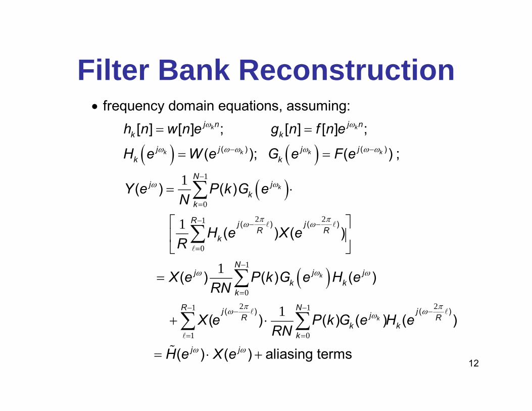
Filter Bank Reconstruction
( ) ( )( )
1
0
2 21
0
1
1
1
( ) ( )
( ) ( )
frequency domain equations, assuming: [ ] [ ] ; [ ] [ ] ;
( ); ( ) ;
( ) ( )
( ) ( )
( )
k k
k k k k
k
j n j nk k
j j j jk k
Njj
kk
R j jR R
k
j
h n w n e g n f n e
H e W e G e F e
Y e P k G eN
H e X eR
X e
ω ω
ω ω ω ω ω ω
ωω
π πω ω
ω
− −
−
=
− − −
=
•
= =
= =
= ⋅
⎡ ⎤⎢ ⎥⎣ ⎦
=
∑
∑l l
l
( )1
0
2 21 1
1 0
1( ) ( )
( ) ( )
( ) ( ) ( ) ( )
( ) ( ) aliasing terms
k
k
Nj j
k kk
R Nj jjR Rk k
k
j j
P k G e H eRN
X e P k G e H eRN
H e X e
ω ω
π πω ωω
ω ω
−
=
− −− −
= =
+ ⋅
= ⋅ +
∑
∑ ∑l l
l
%

13
Filter Bank Reconstruction
1
0
21
0
1 1
1 0 1 2( )
ˆ conditions for perfect reconstruction ( ( ) ( ))
( ) ( ) ( ) ( )
and
( ) ( ) ( ) for , ,...,
k
k
j j
Njj j
k kk
N jj Rk k
k
Y e X e
H e P k G e H eRN
P k G e H e RRN
ω ω
ωω ω
πωω
−
=
− −
=
• =
= =
= =
∑
∑l
%
l
Flat Gain
Alias Cancellation

Filter Bank Reconstruction
14

15
Decimated Analysis-Synthesis Filter Bank
2
1 0 1 14
1 04
( ) ( )
( )
practical solution for the case ( ) ( ), (2-band solution)where the conditions for exact reconstruction become
( ) ( ) ( ) ( ) ( ) ( )
and
( ) ( ) (
ω ω ω π ω π
ω ω π
− −
−
• = = =
⎡ ⎤+ =⎣ ⎦j j j j
j j
w n f n N R
P F e W e P F e W e
P F e W e
( ) ( )
2
2 2
1 0
0 1 114
( ) ( )
( )
) ( ) ( ) ( )
aliasing cancels exactly if ( ) ( ) (with ( ) ( ))giving
( ) ( )
ˆ( ) ( )
ω π ω π
ω ω
ω ω π ω
− −
− −
⎡ ⎤+ =⎣ ⎦
• = − = =
⎡ ⎤− =⎢ ⎥⎣ ⎦= −
j j
j j
j j j M
P F e W e
P P F e W e
W e W e e
y n x n M

Decimated Analysis-Synthesis Filter Bank
16
1( )
0
1( ) [ ] ( )
( ) ( ) ( )
when aliasing is completely eliminated (by suitable choice of filters),the overall analysis-synthesis system has frequency response:
where
ω ωω
ω ω ω
−−
=
=
=
∑%
%
k
Njj
ek
j j je
H e P k W eRN
W e W e F e
h
1
0
[ ] [ ] [ ]
[ ] [ ] [ ]1[ ] [ ]
where
ω−
=
=
= ∗
= ∑ k
e
eN
j n
k
n w n p n
w n w n f n
p n P k eRN
Decimated Analysis-Synthesis Filter Bank
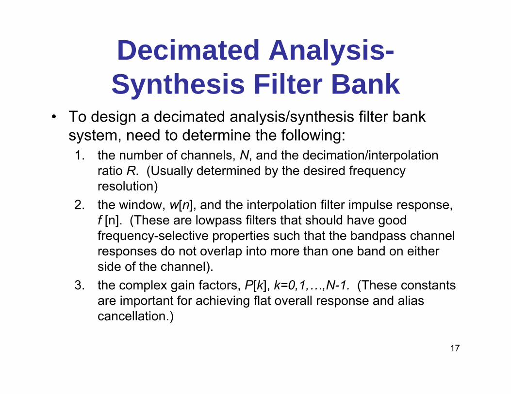
• To design a decimated analysis/synthesis filter bank system, need to determine the following:1. the number of channels, N, and the decimation/interpolation
ratio R. (Usually determined by the desired frequency resolution)
2. the window, w[n], and the interpolation filter impulse response, f [n]. (These are lowpass filters that should have good frequency-selective properties such that the bandpass channel responses do not overlap into more than one band on either side of the channel).
3. the complex gain factors, P[k], k=0,1,…,N-1. (These constants are important for achieving flat overall response and alias cancellation.)
17

Maximally Decimated Filter Banks
• we show here that it is possible to obtain exact reconstruction with R=N and N<L.– R=N is termed maximal decimation because this is the
largest decimation factor that can be used with an N-channel filter bank and still achieve exact reconstruction.
– nominal bandwidth of the bandpass channel signal is increased from ±π/N to ±π
– down-sampling by N accomplishes frequency down-shifting normally accomplished by modulation
18
Maximally Decimated Filter Banks
19

Analysis-Synthesis Filter Bank (all modulators removed)
20

Two Channel Filter Banks
21

Two Channel Filter Banks
22
0 0 1 1
( ) ( )0 0 1 1
2; , 0,1
1( ) ( ) ( ) ( ) ( ) ( )21 ( ) ( ) ( ) ( )2
For this two-band system, we have: Applying the frequency domain analysis we get:
ω ω ω ω ω ω
ω ω π ω ω π
ω π
− −
= = = =
⎡ ⎤= +⎣ ⎦
⎡+ +
k
j j j j j j
j j j j
R N k k
Y e G e H e G e H e X e
G e H e G e H e ( )
( ) ( )0 0 1 1
( )
1/ [0], [1]
( ) ( ) ( ) ( ) 0
not including multiplier or the gain factors Aliasing can be eliminated completely by choosing the filters such that:
(ali
ω π
ω ω π ω ω π
−
− −
⎤⎣ ⎦
⎡ ⎤+ =⎣ ⎦
j
j j j j
X e
N P P
G e H e G e H e
0 0 1 11 ( ) ( ) ( ) ( ) 1 (2
asing cancelation)
Perfect reconstruction requires:
flat gain condition)ω ω ω ω⎡ ⎤+ =⎣ ⎦j j j jG e H e G e H e

Quadrature Mirror Filter (QMF) Banks
23
( )1 0 1 0
0 0 0 0
( )1 1 1 0
[ ] [ ] ( ) ( )
[ ] 2 [ ] ( ) 2 ( )
[ ] 2 [ ] ( ) 2 ( )
Alias cancellation achieved if the filters are chosen to satisfythe conditions:
Note that the
j n j j
j j
j j
h n e h n H e H e
g n h n G e H e
g n h n G e H e
π ω ω π
ω ω
ω ω π
−
−
= ⇔ =
= ⇔ =
= − ⇔ = −
0[ ]re is only a single lowpass filter, with impulse response
on which all other filters are based; filter has nominal cutoff of /2 rad with a narrow transition to a stopband with adequate attenuat
h nπ
1 0
0 1
[ ] [ ][ ] [ ]
ionto isolate the two bands The filter is the complementary highpass filter The filters and are called Quadrature Mirror Filters (QMF)
j nh n e h nh n h n
π=

Quadrature Mirror Filter (QMF) Banks
24
( ) ( )
( ) ( ) ( 2 )0 0 0 0
2 2( )0 0
2 ( ) ( ) 2 ( ) ( ) 0
( ) ( ) ( )
Substituting for the filter relationships we get: i.e., perfect alias cancellation for any choice of lowpass filter
ω ω π ω π ω π
ω ω ω π
− − −
−
− =
= −
j j j j
j j j
H e H e H e H e
Y e H e H e
( ) ( )2 2( )0 0
( ) ( ) ( )
( ) ( )
For perfect reconstruction we require that:
i.e., flat magnitude with delay of samples, due to the delayof the causal filters of the filte
ω ω ω
ω ω π ω− −
⎡ ⎤ =⎢ ⎥⎣ ⎦
⎡ ⎤− =⎢ ⎥⎣ ⎦
%j j j
j j j M
X e H e X e
H e H e e
Mr bank
Quadrature Mirror Filters
25
0 0
0 0
[ ] [( 1) ], 0 1;( 1) / 2
( ) (
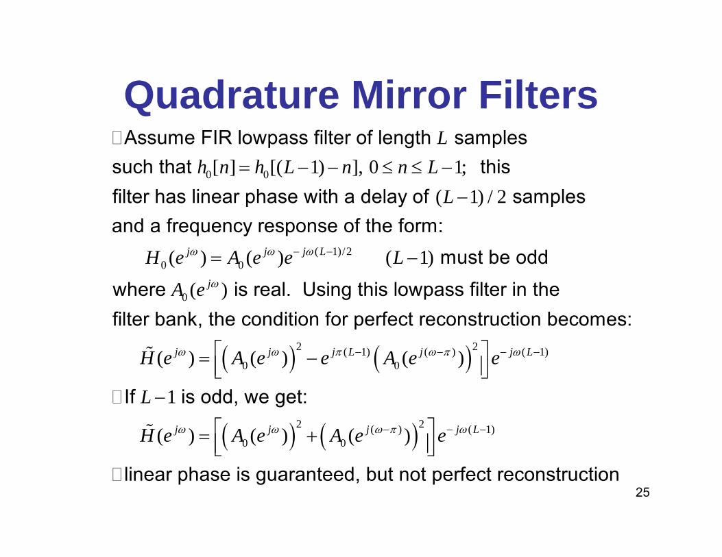
Assume FIR lowpass filter of length samplessuch that thisfilter has linear phase with a delay of samplesand a frequency response of the form: j j
Lh n h L n n L
L
H e A eω
= − − ≤ ≤ −−
=
( ) ( )
( 1)/2
0
2 2( 1) ( )0 0
) ( 1)
( )
( ) ( ) ( )
must be oddwhere is real. Using this lowpass filter in thefilter bank, the condition for perfect reconstruction becomes:
j L
j
j j j L j j
e L
A e
H e A e e A e e
ω ω
ω
ω ω π ω π ω
− −
− − −
−
⎡ ⎤= −⎢ ⎥⎣ ⎦%
( ) ( )
( 1)
2 2( ) ( 1)0 0
1
( ) ( ) ( )
If is odd, we get:
linear phase is guaranteed, but not perfect reconstruction
L
j j j j L
L
H e A e A e eω ω ω π ω
−
− − −
−
⎡ ⎤= +⎢ ⎥⎣ ⎦%

Quadrature Mirror Filters
26
( ) ( )2 2( )0 0( ) ( ) 1
For flat gain we need to satisfy the condition:
Solution is to use high order linear phase QMF filters Johnston proposed an algorithm for design of the basic
lowpass fi
j jA e A eω ω π−⎡ ⎤+ =⎢ ⎥⎣ ⎦
lter that minimized the deviation from unity while providing a desired level of stopband attenuation

27
Quadrature Mirror Filters
0 0[ ] [ ] [ ]= =h n w n g n 1 1[ ] [ ] [ ]π= =j nh n w n e g n

28
Quadrature Mirror Filters
• practical realization of QMF filters
• note that aliasing is cancelled, but the overall frequency response is not perfectly flat
Lowpass filter designed by windowing
Highpass filter is mirror image of lowpass filter

Quadrature Mirror Filters
29

30
• The motivation for the subband approach is to process different speech properties independently in each band and thus being able to localize the band (compact bandwidth) is important.
• Also,based on the original motivation of short-time analysis, temporal focus (within a limited time duration) is also important.
• Filter bank design is thus result of a trade-off between perfect reconstruction and bandwidth concentration in a joint criterion:
• When processing (e.g., quantization, a non-linear operation) is involved, harmonic distortions are inevitable and perfect reconstruction cannot be achieved, as seen in the simple example.
• There exists a design procedure (Smith-Barnwell) for QMF filters that attempts to meet the design constraints as best as possible
Issues with Perfect Reconstruction
∫∫ −−+=π ωπ
ω
ω ωαωα0
22 )|)(|1()1(|)(| deTdeWJ jj
s
Stop-band leakage Deviation from PR

31
1. Start with a sequence of length, say, 2L-1 (L even) that satisfiesthat is, even samples=0, except at n=0.
, the value of the sequence at n=0, needs to be large enough to satisfy the positivity condition (see below).
2. Factorsuch that all roots of are inside the unit circle.
3. Positivity condition:4. The mirror channel:
5. To eliminate aliasing:
Smith-Barnwell QMF Design
{ } )()()()( 100
−== zWzWngzG Z
0C);(2)()1()( 0 nCngng n δ=−+
)( zW
0)()()()(2
000 >== − ωωωω jjjj eWeWeWeG
1,)()( 01 −=−−= −− LNeeWeW Njjj ωωω
)()1()(ly equivalentor )()( 011
01 nNwnwzzWzW nN −−=−−= −−
)()1()(ly equivalentor )()( 1010 nwnfzWzF n−=−=)()1()(ly equivalentor )()( 0101 nwnfzWzF n−−=−−=
)()( and )()( 0110 zWzFzWzF −−=−=

32
Smith-Barnwell QMF Design - Example
condition positivity esatisfy th toadded is 0.1 0,at =n
12length has )( then ,)( ofLength 0 −= LngLnw7,,2,1,0,)2/sin()( ±±±== Ln
nnng
ππ
0.0455]- 0.0000 0.0637 0.0000- 0.1061- 0.0000 0.3183 0.6 0.3183 0.0000 0.1061- 0.0000- 0.0637 0.0000 -0.0455[)( =ng
L = 8, N = L – 1 = 7
choose
{ } )()()()( 100
−== zWzWngzG Z
Factorize )()()( 100
−= zWzWzG
0.1461]- 0.1182 0.1590 0.2032- 0.2332- 0.3426 0.8091 1[)(0 =nw
circleunit theinside roots all with length :(z)0 LW
1]- 0.8091 0.3426- 0.2332- 0.2032 0.1590 0.1182- -0.1461[)()1()( 01 =−−= nNwnw n
1] 0.8091 0.3426 0.2332- 0.2032- 0.1590 0.1182 -0.1461[)()1()( 10 =−= nwnf n
0.1461]- 0.1182- 0.1590 0.2032 0.2332- 0.3426- 0.8091 1[)()1()( 01 −=−−= nwnf n
all arrays start with n=0

33
QMF Frequency Responses (Example)
Normalized frequency (xπ)
1050
-5-10-15-20
20
-2-4-6-8
-10-12
Mag
nitu
de (d
B)
Pha
se(d
egre
e, x
100)

Tree-Structured Filter Banks
34

Tree-Structured Filter Banks
35

Sampling Pattern for Tree-Structured Filter Banks
36
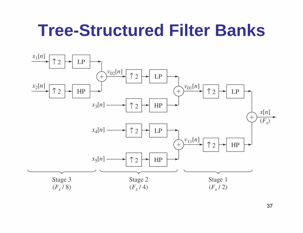
Tree-Structured Filter Banks
37
38
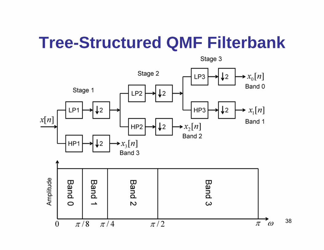
Tree-Structured QMF Filterbank

39
Quantization noise is concentrated in the band that it is generated in.
Quantized Channel Signals
][ˆ0 ny
][ˆ1 ny
][ˆ ny
]1[ −nδ
]1[ −nδ][nδ
][nδ
][0 nh 2↓ 2↑ ][0 ng
][1 nh 2↓ 2↑ ][1 ng
][0 ne
][1 ne
0 1
2 20 1ˆ ( ) ( ) ( )ω ω ωσ σ= +j j j
e eyP e G e G e

40
Subband Coding
• advantages of subband coding
• each subband can be encoded according to the perceptual criterion appropriate to that band
• quantization noise can be confined to the band that produces it
• low energy bands can be encoded so as to produce less noise
• applicable to coding in the 9.6-16 Kbps range
41
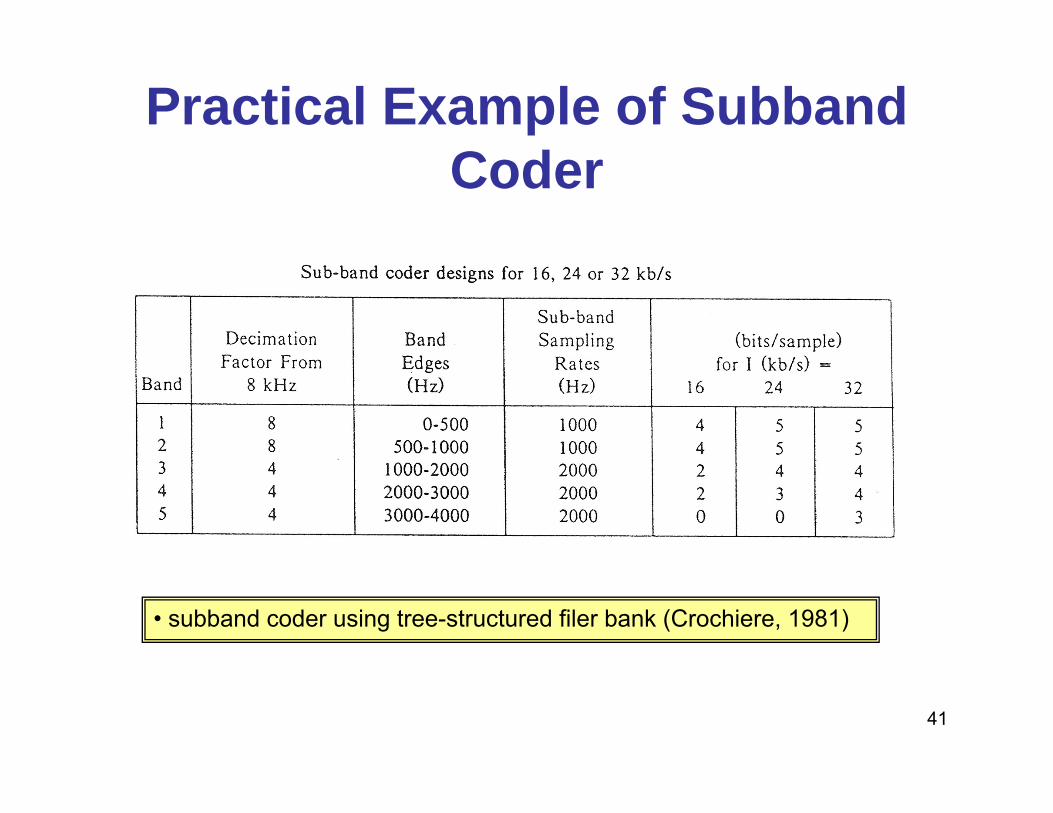
Practical Example of Subband Coder
• subband coder using tree-structured filer bank (Crochiere, 1981)

42
Subband Coder Subjective Quality

43
Subband Coder Waveforms

44
Concept of Time-Frequency Resolution• When interested in the changing characteristics of the signal,
short time Fourier transform or short time spectral analysis is used.
12222
12222
|)(||)(|)(
|)(||)(|)(
−∞
∞−
∞
∞−
−∞
∞−
∞
∞−
⎥⎦⎤
⎢⎣⎡•−=
⎥⎦⎤
⎢⎣⎡•−=
∫∫
∫∫
ωωωωωωσ
σ
ω dGdG
dttgdttgtt
c
ct
:spreadFrequency
:spread Temporal
τττω ωτdetgftF j∫∞
∞−
−−= )()(),(time. in focus providing function window the is )(tg
Continuous prolate spheroidal wave function: a bandlimited signal that have the highest energy concentration in a specified time interval.
.5.0)(=ωσσ t
tg product bandwidth-time minimum the achieves it Gaussian, is If
• To maintain a similar level of uncertainty, the window function should be short to provide time resolution for high frequency components and long to provide frequency resolution for low frequency components.

45
Wavelet-Based MethodsAnalysis Filters Synthesis Filters
Band 1 ↓ R Q Q-1 ↑ R Band 1
Band 2 ↓ R Q Q-1 ↑ R Band 2
Band N ↓ R Q Q-1 ↑ R Band N
. . . . . . . .
Subband method
Analysis Filters Synthesis Filters
↓ R Q Q-1 ↑ R
↓ R Q Q-1 ↑ R
↓ R Q Q-1 ↑ R
Wavelet method
WaveletTransform
InverseTransform
What is in the Wavelet Transform block? What is the difference?

46
Wavelet Transform• Built on set of expansion (or basis) functions that are
derived from a mother wavelet through scaling and translation:
∞<Ψ
= ∫∞
0
20 |)(| ωωω
ψ dC
)}({)}({ ,, tt aa ττ ψωψω F)( and F)( Let =Ψ=Ψ
: waveletmother a be Let )(tψ ⎟⎠⎞
⎜⎝⎛ −
=a
ta
taτψψ τ
1)(,
Continuous Wavelet Transform:
⎟⎟⎠
⎞⎜⎜⎝
⎛−=⎟⎟
⎠
⎞⎜⎜⎝
⎛ −== ∫∫
∞
∞−
∞
∞− af
adt
attf
adtttfaF aw
τψττψψτ τ***
, *)(1)(1)()(),(
Inverse transform: ∫ ∫∞
∞−
∞
∞−= 2, )(),(1)(
adadtaF
Ctf aw
τψτ τψ
00 =Ψ )(
analysis for signal the compress or stretch∫∞
∞−⎟⎠⎞
⎜⎝⎛ −= dt
atatf
aaFw
τψτ *)(1),(
mspectrogra scalogram; == 22 |),(||),(| τωτ FaFw
Admissibility condition:

47
Wavelet and Fourier Transform
⎟⎠⎞
⎜⎝⎛ −=⎟
⎠⎞
⎜⎝⎛ −
= ∫∞
∞− af
adt
attf
aaFw
τψττψτ ** *)(1)(1),(
)}({)}({ ,, tt aa ττ ψωψω F)( and F)( =Ψ=Ψ )}({ tfF F)( =ω
τωττ ωωτψψ j
aa eaaa
ta
t −Ψ=Ψ⇔⎟⎠⎞
⎜⎝⎛ −
= )()(1)( ,,
)()(*)(1)),((),( * ωωτψττω aFaa
fa
aFaW w Ψ=⎭⎬⎫
⎩⎨⎧
⎟⎠⎞
⎜⎝⎛−== FF
transform. waveletthe of tionrepresenta domainfrequency the is ),( ωaW
48
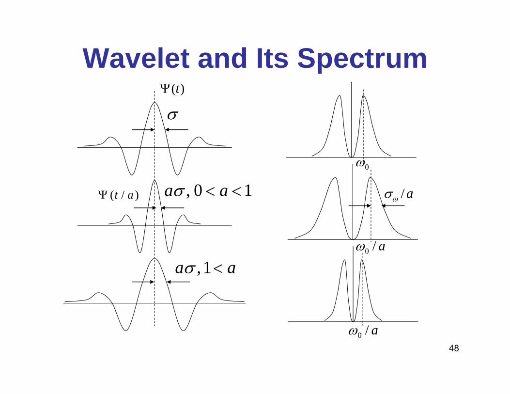
Wavelet and Its Spectrum
)/( atΨ
σ
aa <1,σ
10, << aaσ0ω
a/0ω
a/0ω
a/ωσ
)(tΨ

49
Scaling and Translation• For discrete wavelet transform,
mm anaa −− == 000 ττ and
,12 00 == τ and If a
and
m, n are integers
Znmntaatt mmnma ∈−== ,)()()( 00
2/0,, τψψψ τ
Znmntt mmnm ∈−= ,)2(2)( 2/
, ψψ
wavelets.affine called is it complete, is set the If )}({ , tnmψ
∫∞
∞−−== dtntatfawaF mm
nmw )()(),( 002/
0, τψτ
∑∑=m n
nmnm twtf )()( ,, ψ
*, ,( ) ( ) ( ) ( )Orthogonality condition : m n p qt t dt m p n qψ ψ δ δ
∞
−∞= − −∫
The orthogonality condition may not be easy to satisfy for a general set of “wavelets;” but it is still possible to invert discrete wavelet transform, sometimes.
dyadic or octave sampling

50
STFT and CWT
0ω 05ω03ω 08ω04ω0ω 02ω
time
frequ
ency
timefre
quen
cy
Constant-Q bandwidthConstant bandwidth
51
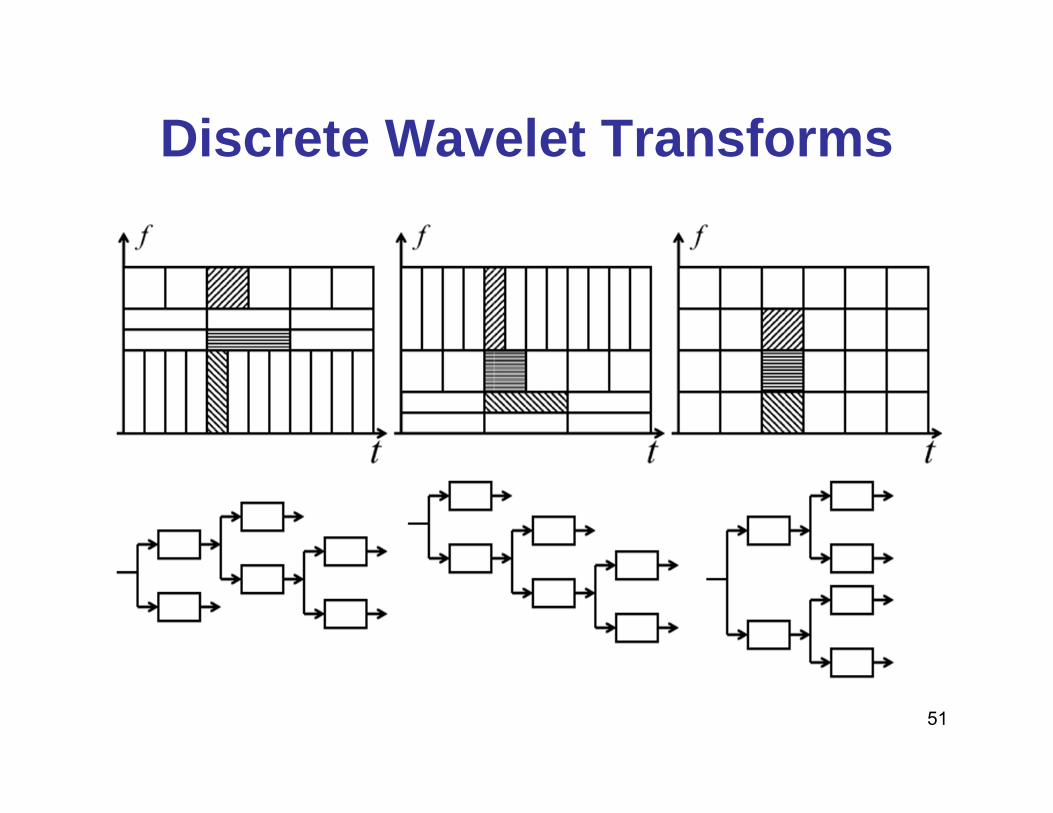
Discrete Wavelet Transforms

52
Other Simpler Transforms or Filter Banks
• Short-time analysis can also be viewed as data transformation, executed in a block-by-block manner, using for example:– Discrete Cosine Transform– Discrete Sine Transform– Filter bank based on DFT/FFT
• General remarks:– Discussion so far aims at a filter bank framework that allows perfect
reconstruction (i.e., no loss of information in the original signal if desired);
– But many speech processing systems do not require perfect reconstruction; rather, one may want to focus on “extraction” of key parameters or features from the speech signal;
– Therefore, other analysis methods (e.g., transformations that do not have inverse) may still apply.

53
DFT and DCTN-point DFT (Discrete Fourier Transform)
Relates to real part of 2N-point DFT when the signal is symmetric
implies
2N-pointsymmetric
2N-point DFTN-point DCT
Possible excessive discontinuity at edges
∑∑−
=
−
=
− =→−==1
0
12
0
)/2( )/2cos()(2)()2()( and )()(N
n
N
n
knNj NknnxkXnNxnxenxkX ππ
∑−
=
−=1
0
)/2()()(N
n
knNjenxkX π
But, be careful about the point of symmetry!!
∑∑∞
−∞=
−
=
+==r
N
k
knNjkNj rNnxeeXN
nx )()(1)(~ 1
0
)/2()/2( ππ
54
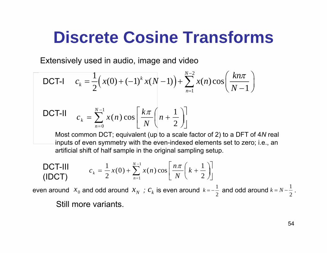
even around and odd around ; is even around and odd around .
Discrete Cosine Transforms
This image cannot currently be displayed.
∑−
=⎥⎦
⎤⎢⎣
⎡⎟⎠⎞
⎜⎝⎛ +=
1
0 21cos)(
N
nk n
Nknxc π
∑−
=⎥⎦
⎤⎢⎣
⎡⎟⎠⎞
⎜⎝⎛ ++=
1
1 21cos)()0(
21 N
nk k
Nnnxxc π
DCT-I ( )2
1
1 (0) ( 1) ( 1) ( ) cos2 1
Nk
kn
knc x x N x nNπ−
=
⎛ ⎞= + − − + ⎜ ⎟−⎝ ⎠∑
DCT-II
Most common DCT; equivalent (up to a scale factor of 2) to a DFT of 4N real inputs of even symmetry with the even-indexed elements set to zero; i.e., an artificial shift of half sample in the original sampling setup.
DCT-III(IDCT)
0x Nx21
−=kkc21
−= Nk
Still more variants.
Extensively used in audio, image and video
55
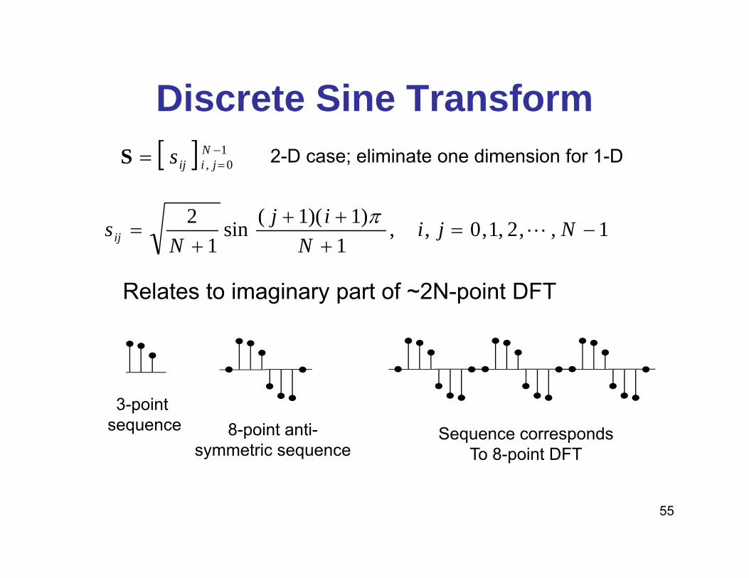
Discrete Sine Transform
1,,2,1,0,,1
)1)(1(sin1
2−=
+++
+= Nji
Nij
Nsij L
π
[ ] 10,
−== N
jiijsS
Relates to imaginary part of ~2N-point DFT
Sequence correspondsTo 8-point DFT
3-point sequence 8-point anti-
symmetric sequence
2-D case; eliminate one dimension for 1-D

56
Discrete (Time) Fourier Transform - Revisited• The DTFT (discrete time Fourier transform) of an N-
point sequence is
• Sample the DTFT at
• The result is the DFT (Discrete Fourier Transform)
• If we compute the inverse DFT, we obtain
ω k = (2π/N)k, k = 0,1,K, N −1.
.continuous is Frequency ω∑−
=
−=1
0)()(
N
n
njj enxeX ωω
∑∑∞
−∞=
−
=
+==r
N
k
knNjkNj rNnxeeXN
nx )()(1)(~ 1
0
)/2()/2( ππ
)()()(1
0
)/2(/2 kXenxeX
N
n
knNjNk
j == ∑−
=
−=
ππω
ω
57
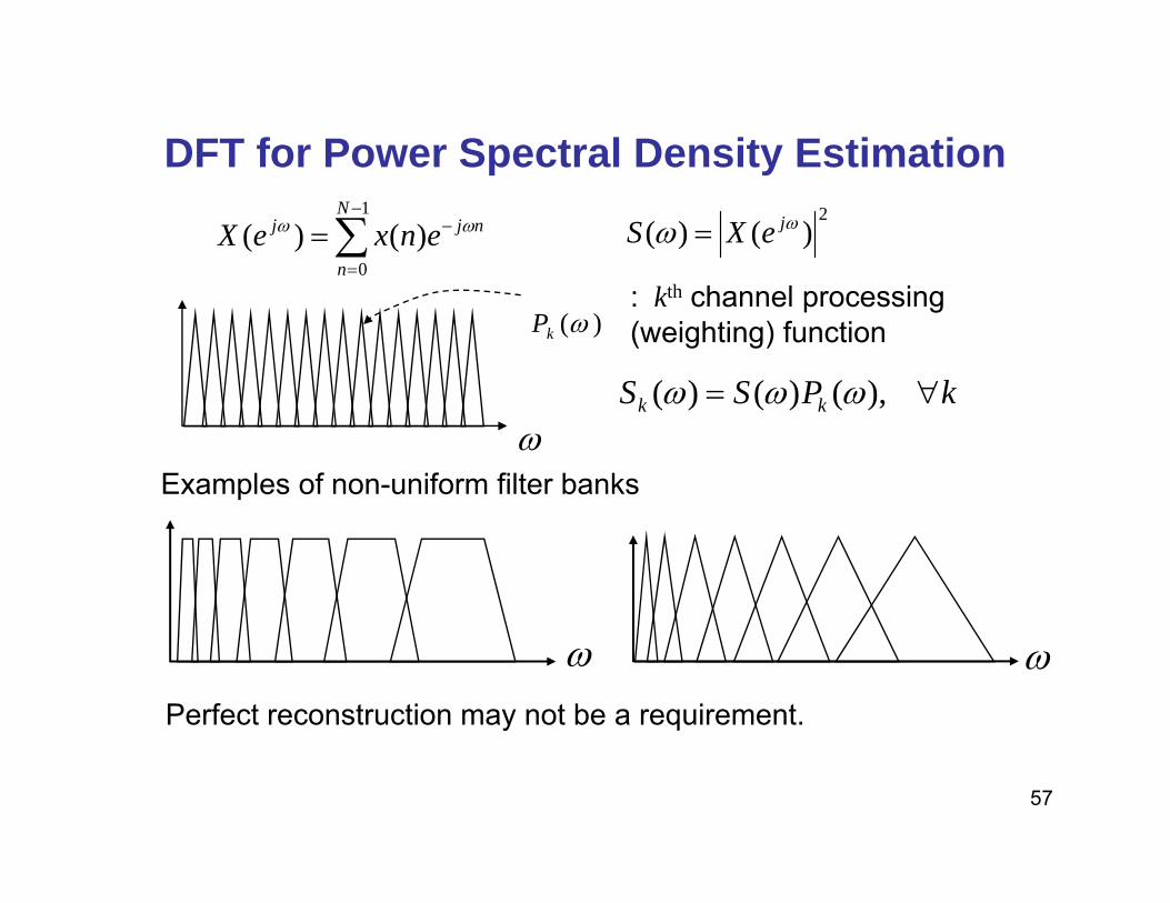
DFT for Power Spectral Density Estimation
∑−
=
−=1
0)()(
N
n
njj enxeX ωω
ω
)(ωkP
2)()( ωω jeXS =
: kth channel processing (weighting) function
kPSS kk ∀= ),()()( ωωω
ωω
Examples of non-uniform filter banks
Perfect reconstruction may not be a requirement.