Behav ResDOI 10.3758/s13428-015-0653-5

Digital LED Pixels: Instructions for useand a characterization of their properties

Pete R. Jones1 · Sara E. Garcia1 ·Marko Nardini1,2

© The Author(s) 2015. This article is published with open access at Springerlink.com

Abstract This article details how to control light emit-ting diodes (LEDs) using an ordinary desktop computer. Bycombining digitally addressable LEDs with an off-the-shelfmicrocontroller (Arduino), multiple LEDs can be controlledindependently and with a high degree of temporal, chro-matic, and luminance precision. The proposed solution issafe (can be powered by a 5-V battery), tested (has beenused in published research), inexpensive (∼ $60 + $2 perLED), highly interoperable (can be controlled by any type ofcomputer/operating system via a USB or Bluetooth connec-tion), requires no prior knowledge of electrical engineering(components simply require plugging together), and useswidely available components for which established helpforums already exist. Matlab code is provided, includinga ‘minimal working example’ of use suitable for use bybeginners. Properties of the recommended LEDs are alsocharacterized, including their response time, luminance pro-file, and color gamut. Based on these, it is shown that theLEDs are highly stable in terms of both luminance andchromaticity, and do not suffer from issues of warm-up,chromatic shift, and slow response times associated withtraditional CRT and LCD monitor technology.

Electronic supplementary material The online version of thisarticle (doi:10.3758/s13428-015-0653-5) contains supplementarymaterial, which is available to authorized users.

� Pete R. Jonesp.r.jones@ucl.ac.uk

1 Institute of Ophthalmology, University College London(UCL), 11-43 Bath Street, London EC1V 9EL, UK

2 Department of Psychology, Durham University, Durham, UK

Keywords Light emitting diode · Arduino · Luminance ·Timing · Color gamut

Introduction

To present visual stimuli, psychophysicists in the 19th and20th century developed many ingenious methods, includingthe use of spinning tops (Maxwell, 1857), shadow-castingby lamps or candles (Mach, 1959; Fry, 1948), and mechan-ical systems in which viewable objects are physicallytranslated in space (Tschermak-Seysenegg, 1939; Howard,2012).

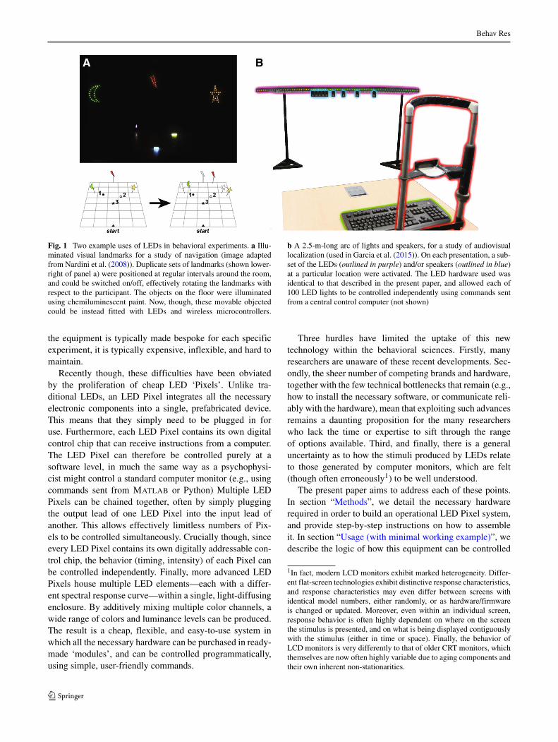
Modern-day scientists typically prefer to use computermonitors to present their visual stimuli. Computer moni-tors are particularly effective at presenting high-resolutionstatic images in the central field. However, they are lesswell suited to other applications; for example, when stim-uli must span the entire visual field, are physically locatedin an interactive 3D environment, or when high temporalprecision is required. In these cases, light emitting diodes(LEDs) can provide a surprisingly simple and effective solu-tion (Nygaard & Frumkes, 1982; Da Silva Pinto et al., 2011;Teikari & et al. 2012; Demontis et al., 2005; Albeanu et al.,2008). For example, in our own research, we have foundLEDs useful for constructing dynamically adjustable land-marks for studying human navigation (Fig. 1a), and forpresenting peripheral stimuli in an audiovisual localizationtask (Fig. 1b).

In the past, many researchers have been discouragedfrom using LEDs because of the level of electrical engi-neering required. Wires must be soldered together, the levelof electrical current must be regulated appropriately, andcontrol circuits must be designed and constructed to pro-duce the specific behavior required. Furthermore, since

Behav Res

A B

Fig. 1 Two example uses of LEDs in behavioral experiments. a Illu-minated visual landmarks for a study of navigation (image adaptedfrom Nardini et al. (2008)). Duplicate sets of landmarks (shown lower-right of panel a) were positioned at regular intervals around the room,and could be switched on/off, effectively rotating the landmarks withrespect to the participant. The objects on the floor were illuminatedusing chemiluminescent paint. Now, though, these movable objectedcould be instead fitted with LEDs and wireless microcontrollers.

b A 2.5-m-long arc of lights and speakers, for a study of audiovisuallocalization (used in Garcia et al. (2015)). On each presentation, a sub-set of the LEDs (outlined in purple) and/or speakers (outlined in blue)at a particular location were activated. The LED hardware used wasidentical to that described in the present paper, and allowed each of100 LED lights to be controlled independently using commands sentfrom a central control computer (not shown)

the equipment is typically made bespoke for each specificexperiment, it is typically expensive, inflexible, and hard tomaintain.

Recently though, these difficulties have been obviatedby the proliferation of cheap LED ‘Pixels’. Unlike tra-ditional LEDs, an LED Pixel integrates all the necessaryelectronic components into a single, prefabricated device.This means that they simply need to be plugged in foruse. Furthermore, each LED Pixel contains its own digitalcontrol chip that can receive instructions from a computer.The LED Pixel can therefore be controlled purely at asoftware level, in much the same way as a psychophysi-cist might control a standard computer monitor (e.g., usingcommands sent from MATLAB or Python) Multiple LEDPixels can be chained together, often by simply pluggingthe output lead of one LED Pixel into the input lead ofanother. This allows effectively limitless numbers of Pix-els to be controlled simultaneously. Crucially though, sinceevery LED Pixel contains its own digitally addressable con-trol chip, the behavior (timing, intensity) of each Pixel canbe controlled independently. Finally, more advanced LEDPixels house multiple LED elements—each with a differ-ent spectral response curve—within a single, light-diffusingenclosure. By additively mixing multiple color channels, awide range of colors and luminance levels can be produced.The result is a cheap, flexible, and easy-to-use system inwhich all the necessary hardware can be purchased in ready-made ‘modules’, and can be controlled programmatically,using simple, user-friendly commands.

Three hurdles have limited the uptake of this newtechnology within the behavioral sciences. Firstly, manyresearchers are unaware of these recent developments. Sec-ondly, the sheer number of competing brands and hardware,together with the few technical bottlenecks that remain (e.g.,how to install the necessary software, or communicate reli-ably with the hardware), mean that exploiting such advancesremains a daunting proposition for the many researcherswho lack the time or expertise to sift through the rangeof options available. Third, and finally, there is a generaluncertainty as to how the stimuli produced by LEDs relateto those generated by computer monitors, which are felt(though often erroneously1) to be well understood.

The present paper aims to address each of these points.In section “Methods”, we detail the necessary hardwarerequired in order to build an operational LED Pixel system,and provide step-by-step instructions on how to assembleit. In section “Usage (with minimal working example)”, wedescribe the logic of how this equipment can be controlled

1In fact, modern LCD monitors exhibit marked heterogeneity. Differ-ent flat-screen technologies exhibit distinctive response characteristics,and response characteristics may even differ between screens withidentical model numbers, either randomly, or as hardware/firmwareis changed or updated. Moreover, even within an individual screen,response behavior is often highly dependent on where on the screenthe stimulus is presented, and on what is being displayed contiguouslywith the stimulus (either in time or space). Finally, the behavior ofLCD monitors is very differently to that of older CRT monitors, whichthemselves are now often highly variable due to aging components andtheir own inherent non-stationarities.

Behav Res

using software, and provide a minimal working example(MWE) of use. Finally, in section “Characterization” wecharacterize the properties of our recommended LEDs, andshow how their luminance, spectral, and timing propertiescompare to those of LCD and CRT monitors.

Methods

Hardware: Overview

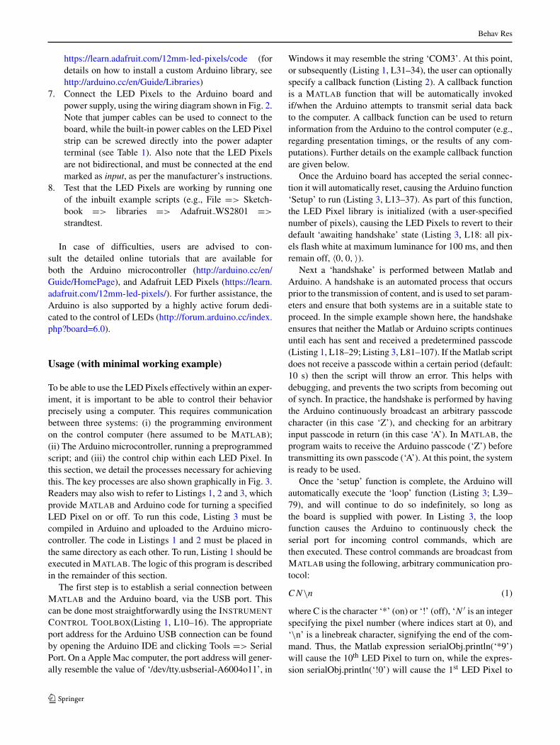
The required hardware is shown graphically in Fig. 2, and islisted in Table 1. The four key pieces of equipment are theLED Pixels, a power supply, an Arduino microcontroller,and a computer. Each of these is described in more detailbelow.

The LED pixels (Fig. 2a)

An LED Pixel consists of one or more LED elements,each connected to an integrated control chip. Multiple LEDPixels can be chained together, but addressed indepen-dently. Although many brands of LED Pixels exist (someof which can be used interchangeably), here we concen-trate on a single product: the Adafruit 12-mm diffused LEDPixels (Adafruit Industries, New York, USA). These werepreferred as they support full 24-bit color, have a reason-ably high modulation rate (2.5 kHz), are well supportedwith an efficient software library and clear instructions,require no technical assembly (e.g., no soldering), and have

proven to be reliable and robust. However, the same basicmethods can be easily adapted to work with other similarproducts.

By default, a strand of Adafruit 12-mm diffused LEDPixels contains 25 independently addressable pixels. Thisnumber can be increased by plugging together multi-ple strands, or reduced if required by simply cutting offunwanted pixels using scissors. Each pixel is composed ofthree independent LED elements (red, green blue) housedwithin a circular diffuser screen (8 mm in diameter), andcontrolled by a 24-bit (8-bit per LED) programmable driverchip (WS2801; Worldsemi Technology, Shenzhen, China).Thus, each pixel can independently display 16.78 million(i.e., 256 x 256 x 256) possible color combinations (seesection “Characterization” for full empirical characteriza-tion). The chipset that drives each pixel uses 2.5-KHz pulsewidth modulation (PWM) to vary luminance (i.e., lumi-nance is controlled by rapidly flickering the light on/off,ideally at a rate beyond that which can be perceived bythe human eye). For further discussion of issues relatingto PWM luminance-modulation, and for users who mayrequire a continuous light source of variable luminance, seethe Supplemental Material (Section S1).

The 5-V power supply (Fig. 2b)

The LED Pixels require a 5-V (± 10 %) input, and eachLED Pixel draws up to 60 mA at maximum luminance. Theinput can be constituted from four 1.2-V batteries, or a 5-V mains adaptor. A mains adaptor is generally preferred for

−+

D C B

A

5V

Fig. 2 Schematic illustration of the key hardware required. a A stripof digitally addressable LED ‘Pixels’. Each pixel consists of threeindependent LEDs (red, green, blue), located behind a diffuser, andcontrolled by an internal chip (WS2801). bA 5-V power supply (either

battery or mains adapter). c An Arduino Uno microcontroller, used tocontrol the LED Pixels. d An ordinary laptop or PC to program, con-trol, and supply power to the Arduino. See body text for details, andTable 1 for further particulars

Behav Res

Table 1 Complete listing of required hardware, including illustrations of example products

Required Hardware

N Image Description

1 Computer

Any latpop or desktop computer with a USB 2.0 connection (or newer).

1 Arduino Microcontroller

A microcontroller, used to interface between the Computer and the

LED Pixel Strand hardware. Any Arduino board is sufficient, but the

current ‘standard’ Uno board is recommended for consistency.

1 USB 2.0 Cable

One male (Type A) to male (Type B) USB 2.0 Cable, to transmit data between

the Computer and Arduino Microcontroller. Also used to supply power

to the Arduino Microcontroller.

1+ LED Pixel Strand

One or more strand of Adafruit 12mm Pixels (25 LEDs per strand).

Multiple strands can be plugged together. First strand must be

connected to the Arduino Microcontroller via Jumper Wires.

To avoid power drain it is recommended that one 5V DC Power Adapter

is used per two strands, although fewer power supplies may be required if not

all LEDs are illuminated at any one time.

4 Jumper Wire

Male-to-male electrical ‘breadboard’ wires, to connect first

LED Pixel Strand with the Arduino Microcontroller (N.B. red

wire only required if drawing power from the board). Alternatively, any ordinary

insulated wire can be used (but will require stripping, and stranded wires may

require tinting to avoid fraying).

1+ 5V Power Adapter

Mains transformer. Recommended one per 50 LEDs. Alternatively can use a battery

power source, or, for a smaller number of LEDs, draw power directly from the 5V

pin on the Arduino Microcontroller.

1+ Power Adapter Terminal

Takes 5V Power Adapter output, and connects to the built-in red

(positive) and blue (negative) wires on the LED Pixel Strand.

One required per 5V Power Adapter.

See Fig. 1 for how these components are assembled, and for further details see the manufacturer’s guide for the Adafruit 21-mm LED Pixels

consistency and ease of maintenance. Inputs greater than5.5 V should not be used, and may permanently damage theLED Pixels. For long strands requiring a large current, mul-tiple 5-V power supplies can be connected at regular inter-vals to limit power drain (see section “Drain and halation”).

If only a small number of LED Pixels are required at anyone time (e.g., two or three), and/or if high luminanceis not required, then the LED Pixels can also draw theirpower directly from the 5-V pin on the Arduino board (i.e.,connecting the red wire to the pin marked “5V” in Fig. 2).

Behav Res

The Arduino microcontroller (Fig. 2c)

A microcontroller is required to interface between the con-trol computer and the LED Pixels (Fig. 2c). We recommendusing the latest Arduino microcontroller, which at the timeof writing is the Arduino Uno (SmartProjects, Strambino,Italy). The code provided here will also work with otherArduino boards, including the older Diecimila and NG vari-ants. However, the limited memory in some other modelscan prove prohibitive for any but the most basic programs(e.g., for any paradigms where arrays of values must bestored on the board). Instead of an Arduino board, thesame basic processes can also be implemented using morepowerful devices, such as the Raspberry Pi (Raspberry PiFoundation, Cambridge, UK), BeagleBone (Texas Instru-ments, Dallas, TX, USA) or PCDuino (LinkSprite Tech-nologies, Longmont, CO, USA). Note, however, that thesedevices are not microcontrollers, but full application proces-sors (miniaturized personal computers), and so can be morecomplicated to set up and use (e.g., requiring the installationand configuration of an operating system). Compared to theArduino boards, they also have less established user groupsand help forums, which will be a substantial limiting factorfor many users.

The computer (Fig. 2d)

A laptop or desktop computer is required to program, andto optionally supply power to, the Arduino microcontroller(see below). Both of these functions are carried out usinga single USB 2.0 cable (see Table 1). The computer is alsogenerally used to control the Arduino during the experiment,via serial commands sent over USB. Alternatively, onceprogrammed the Arduino can be disconnected and usedautonomously (e.g., responding directly to user inputs, suchas button presses, and powered using a battery cell). How-ever, it is generally more convenient to keep the Arduinotethered to a host computer, which can then be used to pro-cess participant responses, synchronize the Arduino withother devices, and/or store experimental data. Almost anycomputer can be used, as long as it supports a USB 2.0 con-nection (see section “Software requirements” for details onoperating systems).

Software requirements

The methods described here should be compatiblewith all operating systems (Windows XP/Vista/7/8, MacOS X, or Linux, all 32 or 64 bit), although usersshould check the official Arduino support documentsif uncertain. We have tested the code given in section“Usage (with minimal working example)” on PCs running

Windows XP andWindows 7, and on variousMacBook Prosrunning OS X 10.4–10.6.

The control computer must be able to run the Arduinoprogramming language (v1.0.6 at time of writing). Thisis a simplified, open-source version of C/C++. Note thatalthough the Arduino code is written on a computer, oncecompiled the code is uploaded onto the Arduino board itselffor execution. Note also that the computer used to programthe board does not necessarily need to be the same computerthat is used subsequently to control the board via serial com-mands, although for simplicity we shall assume that that isthe case.

In addition the control computer must be capable ofsending serial commands to the Arduino over USB. In theexamples given here, we use MATLAB (R2012b, The Math-Works, Natick, MA, USA) to do this, via the INSTRUMENT

CONTROL TOOLBOX. However, the same principles canbe easily adapted to work with any modern programminglanguage (Python, proce55ing, java, c++).

Assembly and installation

1. Purchase the hardware. All components can be pur-chased from most major electronics retailers. The 12-mm diffused LED Pixels can also be purchased directlyfrom www.adafruit.com, which at the time of writingalso sells an Arduino starter kit, containing all othernecessary components. At the time of writing, the totalprice for all hardware (excluding the control computer),is approximately $110 (plus shipping). Each additionalstrand of 25 LED Pixels costs a further $50 (includ-ing additional power supplies for every 3rd strand,although these may not be needed if high luminance anduniformity are not required)

2. Install the Arduino software on a computer with a USB2.0 connection (or newer).

3. Connect the Arduino board to the computer via a USBcable

4. Configure the Arduino software appropriately, byticking the appropriate item under “Tools =>

Board”, and under “Tools => Serial Port”. Onsome machines—most notably Macbook Pro laptops—no serial port will be listed. In this case, it maybe necessary to install Virtual Com Port [VCP]drivers. At the time of writing, free versions of thesedrivers can be found at: http://www.ftdichip.com/Drivers/VCP.htm

5. Check that the Arduino is functioning properly by run-ning one of the inbuilt example scripts (e.g., File =>

Examples => 01.Basics => Blink)6. Install the necessary LED Pixel library

(“Adafruit WS2801”), which can be downloaded from

Behav Res

https://learn.adafruit.com/12mm-led-pixels/code (fordetails on how to install a custom Arduino library, seehttp://arduino.cc/en/Guide/Libraries)

7. Connect the LED Pixels to the Arduino board andpower supply, using the wiring diagram shown in Fig. 2.Note that jumper cables can be used to connect to theboard, while the built-in power cables on the LED Pixelstrip can be screwed directly into the power adapterterminal (see Table 1). Also note that the LED Pixelsare not bidirectional, and must be connected at the endmarked as input, as per the manufacturer’s instructions.

8. Test that the LED Pixels are working by running oneof the inbuilt example scripts (e.g., File => Sketch-book => libraries => Adafruit WS2801 =>

strandtest.

In case of difficulties, users are advised to con-sult the detailed online tutorials that are available forboth the Arduino microcontroller (http://arduino.cc/en/Guide/HomePage), and Adafruit LED Pixels (https://learn.adafruit.com/12mm-led-pixels/). For further assistance, theArduino is also supported by a highly active forum dedi-cated to the control of LEDs (http://forum.arduino.cc/index.php?board=6.0).

Usage (with minimal working example)

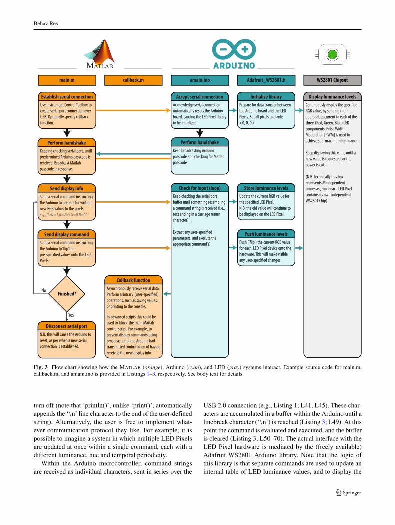
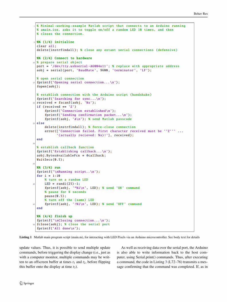
To be able to use the LED Pixels effectively within an exper-iment, it is important to be able to control their behaviorprecisely using a computer. This requires communicationbetween three systems: (i) the programming environmenton the control computer (here assumed to be MATLAB);(ii) The Arduino microcontroller, running a preprogrammedscript; and (iii) the control chip within each LED Pixel. Inthis section, we detail the processes necessary for achievingthis. The key processes are also shown graphically in Fig. 3.Readers may also wish to refer to Listings 1, 2 and 3, whichprovide MATLAB and Arduino code for turning a specifiedLED Pixel on or off. To run this code, Listing 3 must becompiled in Arduino and uploaded to the Arduino micro-controller. The code in Listings 1 and 2 must be placed inthe same directory as each other. To run, Listing 1 should beexecuted in MATLAB. The logic of this program is describedin the remainder of this section.

The first step is to establish a serial connection betweenMATLAB and the Arduino board, via the USB port. Thiscan be done most straightforwardly using the INSTRUMENT

CONTROL TOOLBOX(Listing 1, L10–16). The appropriateport address for the Arduino USB connection can be foundby opening the Arduino IDE and clicking Tools => SerialPort. On a Apple Mac computer, the port address will gener-ally resemble the value of ‘/dev/tty.usbserial-A6004o11’, in

Windows it may resemble the string ‘COM3’. At this point,or subsequently (Listing 1, L31–34), the user can optionallyspecify a callback function (Listing 2). A callback functionis a MATLAB function that will be automatically invokedif/when the Arduino attempts to transmit serial data backto the computer. A callback function can be used to returninformation from the Arduino to the control computer (e.g.,regarding presentation timings, or the results of any com-putations). Further details on the example callback functionare given below.

Once the Arduino board has accepted the serial connec-tion it will automatically reset, causing the Arduino function‘Setup’ to run (Listing 3, L13–37). As part of this function,the LED Pixel library is initialized (with a user-specifiednumber of pixels), causing the LED Pixels to revert to theirdefault ‘awaiting handshake’ state (Listing 3, L18: all pix-els flash white at maximum luminance for 100 ms, and thenremain off, 〈0, 0, 〉).

Next a ‘handshake’ is performed between Matlab andArduino. A handshake is an automated process that occursprior to the transmission of content, and is used to set param-eters and ensure that both systems are in a suitable state toproceed. In the simple example shown here, the handshakeensures that neither the Matlab or Arduino scripts continuesuntil each has sent and received a predetermined passcode(Listing 1, L18–29; Listing 3, L81–107). If the Matlab scriptdoes not receive a passcode within a certain period (default:10 s) then the script will throw an error. This helps withdebugging, and prevents the two scripts from becoming outof synch. In practice, the handshake is performed by havingthe Arduino continuously broadcast an arbitrary passcodecharacter (in this case ‘Z’), and checking for an arbitraryinput passcode in return (in this case ‘A’). In MATLAB, theprogram waits to receive the Arduino passcode (‘Z’) beforetransmitting its own passcode (‘A’). At this point, the systemis ready to be used.

Once the ‘setup’ function is complete, the Arduino willautomatically execute the ‘loop’ function (Listing 3; L39–79), and will continue to do so indefinitely, so long asthe board is supplied with power. In Listing 3, the loopfunction causes the Arduino to continuously check theserial port for incoming control commands, which arethen executed. These control commands are broadcast fromMATLAB using the following, arbitrary communication pro-tocol:

CN\n (1)

where C is the character ‘*’ (on) or ‘!’ (off), ‘N ′ is an integerspecifying the pixel number (where indices start at 0), and‘\n’ is a linebreak character, signifying the end of the com-mand. Thus, the Matlab expression serialObj.println(‘*9’)will cause the 10th LED Pixel to turn on, while the expres-sion serialObj.println(‘!0’) will cause the 1st LED Pixel to

Behav Res

Asynchronously receive serial data.

Perform arbitrary

operations, such as saving values,

or printing to the console.

In advanced scripts this could be

used to ‘block’ the main Matlab

control script. For example, to

prevent display commands being

broadcast until the Arduino had

received the new display info.

Callback function

Finished?

Yes

No

MATLAB

Acknowledge serial connection.

Automatically resets the Arduino

board, causing the LED Pixel library

to be initialized.

Accept serial connectionUse Instrument Control Toolbox to

create serial port connection over

USB. Optionally specify callback

function.

Establish serial connectionPrepare for data transfer between

the Arduino board and the LED

Pixels. Set all pixels to blank:

<0, 0, 0>.

Initialize library

RGB value, by sending the

appropriate current to each of the

three (Red, Green, Blue) LED

components. Pulse Width

Modulation [PWM] is used to

achieve sub-maximum luminance.

Keep displaying this value until a

new value is requested, or the

power is cut.

(N.B. Technically this box

represents N independent

processes, since each LED Pixel

contains its own independent

WS2801 Chip)

Display luminance levels

main.m callback.m amain.ino Adafruit_WS2801.h WS2801 Chipset

Keeping checking serial port, until

predermined Arduino passcode is

received. Broadcast Matlab

passcode in response.

Perform handshake

Send a serial command instructing

the Arduino to prepare for writing

new RGB values to the pixels

e.g., ‘LED=1,R=255,G=0,B=55’

Send display info

Send a serial command instructing

Pixels.

Send display command

N.B. this will cause the Arduino to

reset, as per when a new serial

connection is established.

Discconect serial port

Keep broadcasting Arduino

passcode and checking for Matlab

passcode

Perform handshake

Keep checking the serial port

a command string is received (i.e.,

text ending in a carriage return

character).

parameters, and execute the

appropriate command(s).

Check for input (loop)Update the current RGB value for

N.B. the old value will continue to

be displayed on the LED Pixel.

Store luminance levels

for each LED Pixel device onto the

hardware. This will make visible

Push luminance levels

Fig. 3 Flow chart showing how the MATLAB (orange), Arduino (cyan), and LED (gray) systems interact. Example source code for main.m,callback.m, and amain.ino is provided in Listings 1–3, respectively. See body text for details

turn off (note that ‘println()’, unlike ‘print()’, automaticallyappends the ‘\n’ line character to the end of the user-definedstring). Alternatively, the user is free to implement what-ever communication protocol they like. For example, it ispossible to imagine a system in which multiple LED Pixelsare updated at once within a single command, each with adifferent luminance, hue and temporal periodicity.

Within the Arduino microcontroller, command stringsare received as individual characters, sent in series over the

USB 2.0 connection (e.g., Listing 1; L41, L45). These char-acters are accumulated in a buffer within the Arduino until alinebreak character (‘\n’) is reached (Listing 3; L49). At thispoint the command is evaluated and executed, and the bufferis cleared (Listing 3; L50–70). The actual interface with theLED Pixel hardware is mediated by the (freely available)Adafruit WS2801 Arduino library. Note that the logic ofthis library is that separate commands are used to update aninternal table of LED luminance values, and to display the

Behav Res

Listing 1 Matlab main program script (main.m), for interacting with LED Pixels via an Arduino microcontroller. See body text for details

update values. Thus, it is possible to send multiple updatecommands, before triggering the display change (i.e., just aswith a computer monitor, multiple commands may be writ-ten to an offscreen buffer at times t1 and t2, before flippingthis buffer onto the display at time t3).

As well as receiving data over the serial port, the Arduinois also able to write information back to the host com-puter, using Serial.print() commands. Thus, after executinga command, the code in Listing 3 (L72–76) transmits a mes-sage confirming that the command was completed. If, as in

Behav Res

Listing 2 Matlab callback code (callback.m), for receiving data returned over the serial connection from Arduino. See body text for details

Listing 1 (L31–34), a MATLAB callback function was spec-ified, then this will automatically execute on receipt of anyincoming data. In Listing 2, the logic of this code is thesame as in the Arduino Loop() function. Namely, incomingserial data is accumulated in a buffer until a linebreak char-acter is received, at which point the information is processed(in this case by simply printing the message to the MAT-LAB console; Listing 2, L1–33). Note that these callbackcommands are executed asynchronously from the main con-trol script. This means that although the callback code inListing 2 is executed in the same thread as the main script(Listing 1), it can be executed at any time (i.e., callingListing 2 briefly pauses the main MATLAB script, whichthen automatically resumes upon completion). This meansthat the main script does not have to wait to receive theinformation before proceeding (e.g., to the next trial). How-ever, in some circumstances it may be beneficial to forcethe program to pause to await incoming data, for exampleif the Arduino is expected to return important information

that must be saved at the end of each experimental trial.Note also that although in the present example the datareturned from the Arduino is simply printed to the MAT-LAB console, it could equally be saved to a hard disk, orused to directly control the behavior of the main Matlabscript.

Once the main MATLAB experiment script is complete, itcloses the serial connection with the Arduino, and releasesany demands on memory (Listing 1; L48–51). Note thatdisconnecting the serial connection will cause the Arduinoboard to reset and the ”Setup()” function to be executed(Listing 3, L13–37), just as opening the serial connectiondid in step one. In practice, this will cause the LED Pixellibrary to be reinitialized, and all the LED Pixels will beturned off. Because of the use of a handshake step, theArduino script should then remain in the ‘awaiting hand-shake’ phase (Listing 3, L84–107) indefinitely, until a newserial connection is establish and the Arduino script onceagain resets.

Behav Res

Behav Res

Listing 3 Arduino code (amain.iso), for receiving serial commands fromMatlab, controlling LED Pixels accordingly, and returning status updatesto Matlab

Characterization

To characterize the properties of the Adafruit 12mm dif-fused LED Pixels (see section “Hardware: Overview”),measurements of luminance color spectrum, and temporalresponse were made (Leachtenauer, 2004; Brainard et al.,

2002). Details of how recordings were made are givenwithin the relevant subsection. Where stated, analogousrecordings from an example Cathode Ray Tube [CRT] mon-itor (ViewSonic G90fB 19”; ViewSonic Corporation, Brea,CA, United States) and liquid-crystal display [LCD] moni-tor (Samsung SyncMaster 305T 30”; Samsung Electronics

Behav Res

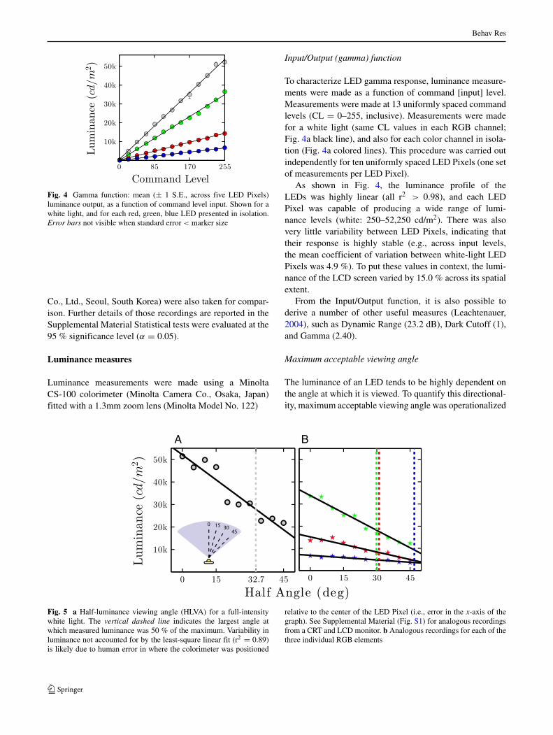
Fig. 4 Gamma function: mean (± 1 S.E., across five LED Pixels)luminance output, as a function of command level input. Shown for awhite light, and for each red, green, blue LED presented in isolation.Error bars not visible when standard error < marker size

Co., Ltd., Seoul, South Korea) were also taken for compar-ison. Further details of those recordings are reported in theSupplemental Material Statistical tests were evaluated at the95 % significance level (α = 0.05).

Luminance measures

Luminance measurements were made using a MinoltaCS-100 colorimeter (Minolta Camera Co., Osaka, Japan)fitted with a 1.3mm zoom lens (Minolta Model No. 122)

Input/Output (gamma) function

To characterize LED gamma response, luminance measure-ments were made as a function of command [input] level.Measurements were made at 13 uniformly spaced commandlevels (CL = 0–255, inclusive). Measurements were madefor a white light (same CL values in each RGB channel;Fig. 4a black line), and also for each color channel in isola-tion (Fig. 4a colored lines). This procedure was carried outindependently for ten uniformly spaced LED Pixels (one setof measurements per LED Pixel).

As shown in Fig. 4, the luminance profile of theLEDs was highly linear (all r2 > 0.98), and each LEDPixel was capable of producing a wide range of lumi-nance levels (white: 250–52,250 cd/m2). There was alsovery little variability between LED Pixels, indicating thattheir response is highly stable (e.g., across input levels,the mean coefficient of variation between white-light LEDPixels was 4.9 %). To put these values in context, the lumi-nance of the LCD screen varied by 15.0 % across its spatialextent.

From the Input/Output function, it is also possible toderive a number of other useful measures (Leachtenauer,2004), such as Dynamic Range (23.2 dB), Dark Cutoff (1),and Gamma (2.40).

Maximum acceptable viewing angle

The luminance of an LED tends to be highly dependent onthe angle at which it is viewed. To quantify this directional-ity, maximum acceptable viewing angle was operationalized

A B

Fig. 5 a Half-luminance viewing angle (HLVA) for a full-intensitywhite light. The vertical dashed line indicates the largest angle atwhich measured luminance was 50 % of the maximum. Variability inluminance not accounted for by the least-square linear fit (r2 = 0.89)is likely due to human error in where the colorimeter was positioned

relative to the center of the LED Pixel (i.e., error in the x-axis of thegraph). See Supplemental Material (Fig. S1) for analogous recordingsfrom a CRT and LCD monitor. b Analogous recordings for each of thethree individual RGB elements

Behav Res

A B

Fig. 6 Drain a and halation b. Markers show mean (± 1 S.E.) luminance for a single LED Pixel (same throughout), as two flanker pixels arebrought progressively closer to the target. See body text for details. See Supplemental Material (Fig. S2) for analogous measurements for eachindividual RGB element

as half luminance viewing angle (HLVA)—the largest angleat which the measured luminance of a full intensity whitelight was 50 % of the maximum (as measured at 0◦). Theresult, shown in Fig. 5a, was HLVA = ± 32.7◦, corres-ponding to a full (left-to-right) span diameter of 65.4◦. Thisrange of viewing angle is approximately half that of theLCD screen (HLVALCD = 62.4◦) and smaller still thanthat of the CRT screen (HLVACRT = 82.5◦)—CRT technol-ogy being highly tolerant of off-angle viewing (Krupinskiet al., 2005). From these results, it can be concluded thata potential limitation of LED Pixels are their directional-ity, making them best suited to situations where the stimuliare never viewed obliquely (e.g., as in Fig. 1b), and/orwhere variations in stimulus intensity are not a concern.The luminance measurements for each individual RGB ele-ment (Fig. 5b) were qualitatively similar to those for a whitelight (R: ± 32.7◦ ; G: ± 29.8◦ , B: ± 46.9◦), and indicateda linear dependency of luminance on viewing angle. Notethat the different slopes for the three color channels meansthat precise hue of any additively mixed colors is liable tovary with viewing angle, though subjectively these varia-tions are not typically salient (see section “Characterizationof chromaticity” for data regarding chromaticity).

Drain and halation

Drain describes a bleeding effect, whereby the luminanceof one LED Pixel is reduced when those around it are

turned on also (i.e., due to a decrease in available current).Drain is a conspicuous problem for most output displays,including LCD and CRT monitors, where dependenciesbetween neighboring regions of the screen can result instimulus artifacts of sufficient magnitude to confound aprecise psychophysical experiment (Garcia-Perez and Peli,2001).

Drain was assessed by measuring output luminance ata fixed, central LED Pixel (the target), as LED Pixels attwo other locations (the flankers) were illuminated withincreasing proximity (as illustrated in Fig. 6). Both targetand flankers were set to maximum luminance throughout(command level = 〈255, 255, 255〉). Drain was quanti-fied as percentage difference to mean target luminancewhen no flankers were present (Fig. 6a, horizontal dashedline). The result is shown in Fig. 6a. Drain effects weresmall but clear, and increased progressively with proxim-ity. When the flankers were relatively distal (global drain),target luminance was reduced by 3.7 %. When the flankerswere immediately adjacent to the target (local drain), targetluminance was reduced by 6.6 %. (N.B. flankers were physi-cally occluded from the colorimeter to prevent measurementconfounds).

Halation is the inverse of drain, whereby a dark (lowluminance) pixel surrounded by bright (high luminance)pixels, exhibits an increase in luminance (i.e., a higherluminance response than would be predicted by the inputcommand level alone (Leachtenauer, 2004)).

Behav Res

As indicated in Fig. 6b, halation was assessed by repeat-ing the drain measurement procedure, but setting the tar-get LED Pixel output to its minimum measurable level(command level = 〈1, 1, 1〉2). Global drain was largelyunchanged, (compared to the previous test using a max-imum level target), but the effects of local drain wereswamped by halation, which resulted in luminance increas-ing by 1.8 % (compared to the 6.6 % decrease due to localdrain, measured previously).

To put these data in context, the just noticeable difference[JND] for detecting a change in luminance is approximately2 % for a white light presented against a dim-photopic back-ground (3–40 cd/m2), rising to around 3 % for a 100 cd/m2

background (comfortable viewing level of a monitor; seeSupplemental Material for more info on typical luminance-detection JND values). The effects of halation reported herewill therefore not be generally apparent to observers, andso will be of little concern for many behavioral scientists.However, the effects of drain may be detectable under closeinspection. If performing stringent psychophysical proce-dures (e.g., where perception of luminance is the measure ofinterest), it would therefore be advisable to correct for thevariations in luminance caused by drain, particularly whenpresenting ‘flanking’ stimuli immediately either side of thetarget.

Moreover, it is important to note that the effects of draincan be exacerbated by increasing the number of flankers.For example, when the number of flankers was increasedto 100 (with a ±10 LED notch around the target), targetluminance decreased by 74 % (Fig. 7, circles). As shownin Fig. 7 (squares), such drain was mitigated but not erad-icated (74 % => 44 %) by connecting a second powersupply to the trailing end of the strand. It is likely that con-necting additional power inputs would have further reduceddrain, but this was not tested. For dense LED Pixel displaysrequiring precise absolute luminance levels, careful cal-ibration, and multiple power supplies, may therefore berequired.

Spectral measures

Spectral measurements were made using a telescopicspectroradiometer (Gamma Scientific, San Diego, CA,USA). Measurements of overall color gamut were alsomade using the CS-100 colorimeter detailed previously(Section “Luminance measures”).

2N.B. Unlike LCD screens, an input of 〈0, 0, 〉 produces no measurableluminance output, and so could not be used to assess the effects ofGlobal Drain.

Fig. 7 Drain effects for increasing dense displays. Each point givesmean (± 1 S.E.) luminance for 12 measurements of the same, ‘target’LED Pixel. Error bars were smaller than marker size in all cases andso are not visible. The target was the central LED Pixel in a strandof 123 LED Pixels. The flanker gap was fixed at ± 10 pixels, andthe number of flankers was varied, with half either side of the target.The target and any flankers were set to maximum luminance (RGB= 〈255, 255, 255〉)

Power spectral density [PSD]

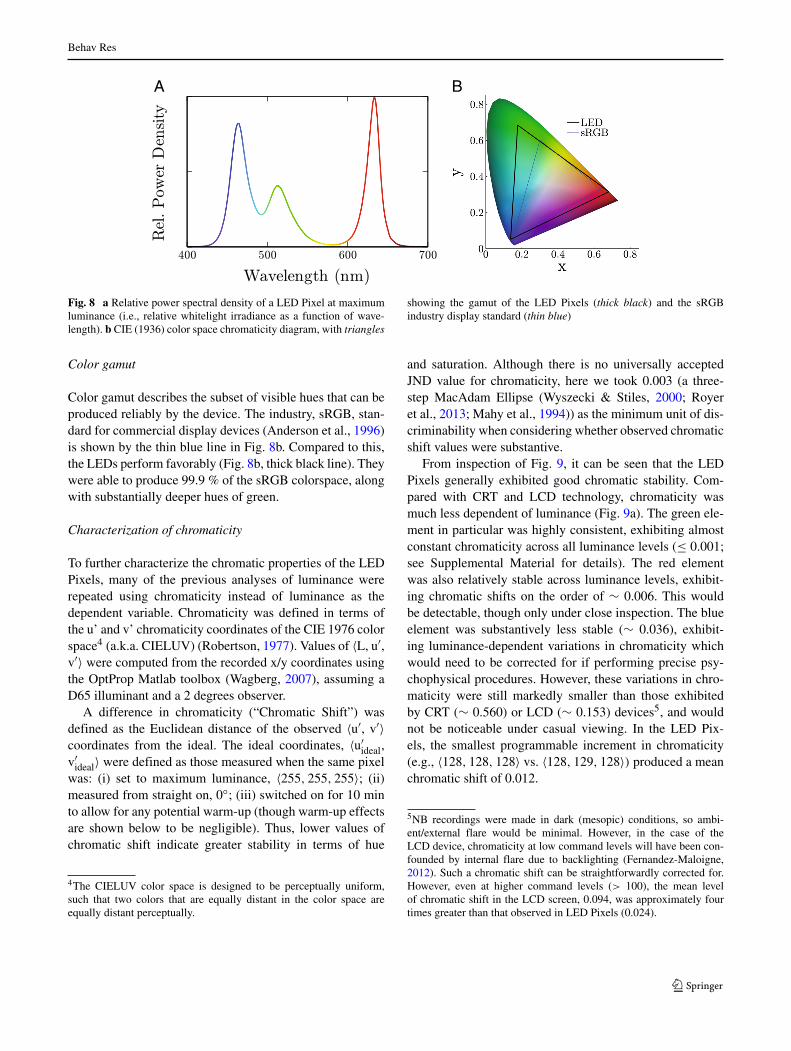
The power spectral density (PSD) of the LED Pixel, mea-sured for a white light at full brightness, is shown in Fig. 8a.Unlike a laser (sinusoidal spectra) or an incandescent bulb(broadband spectra), an LED has a narrowband spectralresponse. The individual response from each of the threeconstituent LEDs is therefore clearly visible in Fig. 8a. Thepeak output wavelengths of the three elements were 464.5,512.3, and 633.4 nm, and they approximately followed nor-mal distributions with standard deviations of 16.7, 25.5, and12.2 nm3 (respectively). This corresponds to full width halfmodulation [FWHM] values of 39.3 (blue), 60.0 (green),and 28.7 nm (red). These response spectra mean, for exam-ple, that the ‘red’ LED element emits extremely little lightbelow 600 nm. Since rod photoreceptors are highly insensi-tive to wavelengths above 600 nm, the ‘red’ LED elementcan therefore be particularly useful for isolating cone func-tionality; for example, in order to monitor residual functionin cone dystrophies such as achromatopsia (Moore, 1992).The width of the spectral power distributions for each ofthe three color channels were similar to those reported pre-viously for CRT phosphers (Brainard, 1989), though the‘blue’ and ‘green’ elements were somewhat more narrowlydistributed.

3Note that the optical bandwidth of a spectroradiometer is liable tobroaden the spectral shape of a measured source. The true values maybe marginally lower.

Behav Res

A B

Fig. 8 a Relative power spectral density of a LED Pixel at maximumluminance (i.e., relative whitelight irradiance as a function of wave-length). b CIE (1936) color space chromaticity diagram, with triangles

showing the gamut of the LED Pixels (thick black) and the sRGBindustry display standard (thin blue)

Color gamut

Color gamut describes the subset of visible hues that can beproduced reliably by the device. The industry, sRGB, stan-dard for commercial display devices (Anderson et al., 1996)is shown by the thin blue line in Fig. 8b. Compared to this,the LEDs perform favorably (Fig. 8b, thick black line). Theywere able to produce 99.9 % of the sRGB colorspace, alongwith substantially deeper hues of green.

Characterization of chromaticity

To further characterize the chromatic properties of the LEDPixels, many of the previous analyses of luminance wererepeated using chromaticity instead of luminance as thedependent variable. Chromaticity was defined in terms ofthe u’ and v’ chromaticity coordinates of the CIE 1976 colorspace4 (a.k.a. CIELUV) (Robertson, 1977). Values of 〈L, u′,v′〉 were computed from the recorded x/y coordinates usingthe OptProp Matlab toolbox (Wagberg, 2007), assuming aD65 illuminant and a 2 degrees observer.

A difference in chromaticity (“Chromatic Shift”) wasdefined as the Euclidean distance of the observed 〈u′, v′〉coordinates from the ideal. The ideal coordinates, 〈u′

ideal,v′ideal〉 were defined as those measured when the same pixel

was: (i) set to maximum luminance, 〈255, 255, 255〉; (ii)measured from straight on, 0◦; (iii) switched on for 10 minto allow for any potential warm-up (though warm-up effectsare shown below to be negligible). Thus, lower values ofchromatic shift indicate greater stability in terms of hue

4The CIELUV color space is designed to be perceptually uniform,such that two colors that are equally distant in the color space areequally distant perceptually.

and saturation. Although there is no universally acceptedJND value for chromaticity, here we took 0.003 (a three-step MacAdam Ellipse (Wyszecki & Stiles, 2000; Royeret al., 2013; Mahy et al., 1994)) as the minimum unit of dis-criminability when considering whether observed chromaticshift values were substantive.

From inspection of Fig. 9, it can be seen that the LEDPixels generally exhibited good chromatic stability. Com-pared with CRT and LCD technology, chromaticity wasmuch less dependent of luminance (Fig. 9a). The green ele-ment in particular was highly consistent, exhibiting almostconstant chromaticity across all luminance levels (≤ 0.001;see Supplemental Material for details). The red elementwas also relatively stable across luminance levels, exhibit-ing chromatic shifts on the order of ∼ 0.006. This wouldbe detectable, though only under close inspection. The blueelement was substantively less stable (∼ 0.036), exhibit-ing luminance-dependent variations in chromaticity whichwould need to be corrected for if performing precise psy-chophysical procedures. However, these variations in chro-maticity were still markedly smaller than those exhibitedby CRT (∼ 0.560) or LCD (∼ 0.153) devices5, and wouldnot be noticeable under casual viewing. In the LED Pix-els, the smallest programmable increment in chromaticity(e.g., 〈128, 128, 128〉 vs. 〈128, 129, 128〉) produced a meanchromatic shift of 0.012.

5NB recordings were made in dark (mesopic) conditions, so ambi-ent/external flare would be minimal. However, in the case of theLCD device, chromaticity at low command levels will have been con-founded by internal flare due to backlighting (Fernandez-Maloigne,2012). Such a chromatic shift can be straightforwardly corrected for.However, even at higher command levels (> 100), the mean levelof chromatic shift in the LCD screen, 0.094, was approximately fourtimes greater than that observed in LED Pixels (0.024).

Behav Res

A B

D E

C

Fig. 9 Changes in LED Pixel chromaticity coordinates (± 1 S.E.) asa function of a input command level, b drain, c halation, d warm-up,and e viewing angle. The out-of-axes markers in (e) indicate additional

measurements made at +70◦. The numeric values for (a) are given inthe Supplemental Material (Table SI)

Effects of drain (Fig. 9b) and halation (Fig. 9x) weregenerally either zero or negligibly small (< 1 JND). Onenotable exception to this overall trend was halation causedby immediately adjacent LED Pixels. Thus, when a max-imally intense white light was presented next to a dimred, green, or blue light, there was some visible distor-tion in the color of dim light. Such effects could beavoided in practice by leaving a one pixel ‘buffer’ aroundvery dim lights. Warm-up times were negligible, with nosystematic variations in chromaticity over time (Fig. 9d),confirming that a warm-up period is not required whenusing LED Pixels. Finally, chromaticity was highly sta-ble with viewing angle for the red and green elements,but was substantive confound for the blue element. Thus,as followed previously from considerations of luminance(section “Maximum acceptable viewing angle”), it wouldbe important to always view the LED Pixels at a constant(e.g., perpendicular) angle if precise stimulus constancywere required.

Temporal measures

Timing measurements were made using a CRS LM03 pho-todiode (Cambridge Research Systems, Cambridge, UK),sampling at a rate of 5 μs.

Response time and onset lag

Response time was measured as the number of millisec-onds taken for the display device to transition from fully offto fully on (black-to-white response time; BWRT), or fromfull on to full off (white-to-black response time; WBRT).As can be seen in Fig. 10a, b, the results from the LEDPixels were indistinguishable from a step function, mean-ing that the response time was virtually instantaneous (<0.001 ms). This compares favorably with the LCD display(BWRT: 7.46 ms; WBRT: 6.68 ms), and is faster even thanthe impulse response time of the CRT (BWRT: 0.58 ms;WBRT: 2.45 ms), details for which are given in the Supple-mental Material (see also Elze and Tanner (2012) for a moredetailed and comprehensive analysis of LCD technology)

A related measure to response time is onset lag: the dura-tion between a command being sent and it being actualizedby the display. This includes both the response time andany other limitations due to transmission speed and refreshrate. From Fig. 10c it can be seen that onset lag was ∼ 6ms. This compares favorably with the typical refresh ratesof an LCD or CRT monitor (60–120 Hz; ∼ 8–16 ms), andmeans that the LED Pixels can be manipulated in near realtime, and with a far higher temporal fidelity that can beachieved using a standard LCD or CRT monitor. The LED

Behav Res

Pixels are therefore well suited to situations where pre-cise control of temporal duration is required—for exampleto maximize responsiveness when designing an interactive(user controlled) display.

There was also very little variability in onset lag acrossrepeated observations (Fig. 10c, d, vs. Figs. S3, S4 inthe Supplemental Material). This means that the temporalresponse of the LED Pixels is not only fast but also highlyreliable/predictable. Such fast and reliable response timesare especially appealing to users looking to synchronize thevisual output with a secondary output, such as an audiodevice.

Refresh rate

An onset lag of 6 ms (see section “Response time and onsetlag”) corresponds to a potential refresh rate of 167 Hz. Thisis already faster than most commercial monitors, which typ-ically operate at 60–120 Hz. Notably though, the 6-ms lag isdue in part to the time taken to encode/transmit/decode com-mands sent in series over the USB port. Thus, even higherrefresh rates can be achieved by sending whole sequencesof commands to the microcontroller in advance (e.g., to beexecuted at specified time in the future, or following a pre-determined trigger). For example, Fig. 11 shows an LEDPixel following a predetermined on/off sequence. Here, arefresh rate of 446 Hz was possible. Thus, LED Pixels mayalso be particularly well suited for experiments that require ahigh flicker rate (Brindley et al., 1966; Simonson & Brozek,1952).

A B

C D

Fig. 10 a, b Response time curves, averaged over 10,000 off-on (a)or on-off (b) transition. Individual measurements were aligned tempo-rally via crosscorrelation prior to averaging. Panels c and d show thedistribution of cross-correlation lag times (i.e., amount of trial-by-triallateral variability in the response curve shown above). The shape of thecurves in the upper panels indicates the response time. The distribu-tions in the lower panels indicate mean onset lag (green vertical line),and variability in onset lag (histograms)

Note, however, that a refresh rate of 446 Hz is an upperlimit, and the maximum refresh rate decreases as the num-ber of LED Pixels increases (N.B. where N is the numberof LED Pixels specified when the WS2801 Arduino libraryis initialized—Listing 3, L9—and not how many LED Pix-els are physically connected). This reduction in refresh rateis because, while it takes the same amount of time to ‘flip’one pixel as it does for an entire strip (the ‘show’ command;Listing 3, L70), luminance update commands are briefly‘held’ by each LED Pixel, and so incur a cumulative timecost (the ‘setPixelColor’ command; Listing 3, L69). As aconsequence, it can take longer than 2 ms (446 Hz) to updatethe luminance levels of even a single LED Pixel if a largenumber of LED Pixels have been specified as addressable.For applications requiring exceptionally high refresh rates(e.g., 446 Hz), therefore only one or two LED Pixels can beaddressed

Warm-up rate

In section “Response time and onset lag” we discussedresponse time: how long it takes for the device to transi-tion from one state (e.g., minimum luminance) to another(e.g., maximum luminance). With traditional visual out-put devices such as CRT and LCD monitors, there isalso a longer-term dynamic in which maximum luminanceincreases gradually for a period after the device is turnedon. Thus, the maximum luminance output of an LCD orCRT screen will be greater after 60 min than it is when firstpowered up for the day, though most of this change typi-cally occurs within the first 5–10 min (Bird, 2010). WithLED technology, such warm-up effects are still a potentialconcern, since the temperature at the junction of the LED

Fig. 11 LED Pixel refresh rates. Curve shows relative luminanceoutput (normalized by dividing by maximum observed level) as a func-tion of time, as a single LED Pixel was turned on/off without anyuser-specified delay. Highlighting shows a single, example sustainedduration, which lasted 2.2 ms

Behav Res

chip can affect forward voltage, and thus the amount of lightemitted.

To examine whether LED warm-up is a practical concernfor behavioral scientists, measurements were made every 30s for LED Pixels that had not been powered in the previ-ous 24 h. The results are shown in Fig. 12, and indicatedthat no warm-up effect was detectable at low (t test compar-ison of linear regression slope to zero: t9 = -2.01, p =.076,n.s.), medium (t9 = 1.05, p =.323, n.s.), or maximum(t9 = -0.94, p = 0.372, n.s.) luminance settings. Thus,while we cannot rule out extremely small, extremely rapid,or extremely gradual effects, warm-up is unlikely to be aconcern when using LED Pixels. This makes them moreconvenient than traditional visual displays (which typicallyneed to be turned on at least 30 min prior to testing whena high degree of precision is required), and eliminates apotential source of measurement error.

Discussion

The present paper describes a simple, cheap, and flexiblesolution for controlling LED light sources, using digitallyaddressable LED Pixels connected to an Arduino microcon-troller. It also details the properties of such a system, interms of output luminance, color, and temporal precision.

In some instances, such a system can provide uniqueadvantages over traditional LCD or CRT monitors. Forexample, LED Pixels were shown to have exceptionally fastand reliable response properties, narrowband color spectra,and a wide dynamic range of luminance levels. Each of

Fig. 12 LED Pixel warm-up dynamics, showing luminance measure-ments for three grey levels (CL= 8, 128, 255), and for each of the threeRGB color elements (CL = 255), as a function of time.Markers showmean (+-SE) luminance levels for each of seven LED Pixels, measuredindependently (error bars not visible when smaller than marker). Linesrepresent least-square regression fits, and did not differ from zero inany case (no change in luminance with time; see body text for details)

these properties may make them appealing for psychophysi-cists, as might their high degree of linearity (which makesthem extremely easy to calibrate and manipulate). For moregeneral users, their ease of use and flexibility may makeLED Pixels an attractive proposition in a range of set-tings. For example, the fact that LED Pixels can be placedanywhere, either in isolation or in clusters, makes themespecially well suited to more ‘ecologically valid’ exper-iments (i.e., where stimuli are presented in a real-worldenvironment, rather than on a screen or headset). As notedby previous authors (Teikari & et al. 2012), LED technologymay also be particularly suited to experiments employingelectrophysiological equipment, due to their relatively lowelectromagnetic interference emissions.

The potential caveats of the LED Pixels were shown tobe their relatively narrow viewing angle (i.e., appearing sub-stantially less bright when viewed eccentrically), and thefact that both timing and luminance properties were depen-dent on the number of LED Pixels used (i.e., the greatestluminance and refresh rates were only possible when usinga single LED Pixel). It should also be noted that the LEDPixels presented here do not support analog (direct current)dimming, though their relatively high PWM means that thiswill not be a limiting factor for the majority of users (see theSupplemental Material for discussion).

The hardware described here is easily extensible. Thenumber of lights can be increased simply by clippingtogether additional LED Pixels. More generally, the basiccomputer/microcontroller setup can also be adapted forqualitatively distinct purposes. For example, previousauthors have detailed more complicated setups in whichan Arduino microcontroller is combined with custom-builtcircuit boards to control both LED elements and incan-descent (civil aviation standard) light bulbs, in order tomodel the effects of different light sources on visual percep-tion and action (Gildea & Milburn, 2013). Furthermore, thesame basic Arduino system (D’Ausilio, 2012) can be eas-ily extended to send and receive data from other devices,including both other forms of outputs (e.g., motors, ser-vos, piezoelectric speakers), as well as various forms ofinput sensors (e.g., temperature, geolocation, galvanic skinresponse, compass direction).

Finally, it is worth stressing that the system describedhere only requires the plugging together of standardized,off-the-shelf components. This makes it a cheap and easy-to-use solution for users with a wide range of technicalexpertise, and the large amount of online support means thatusers are likely to be able to find help if/when problemsoccur.

Acknowledgments The authors thank Gary Rubin, Andrew Stock-man, and Andy Rider for use of equipment, and Aisha McLean forassistance with chromatic measurements. This work was supported by

Behav Res

the Special Trustees of Moorfields Eye Hospital, the NIHR Biomedi-cal Research Centre at Moorfields Eye Hospital and the UCL Instituteof Ophthalmology, and the James S. McDonnell Foundation.

Open Access This article is distributed under the terms ofthe Creative Commons Attribution 4.0 International License(http://creativecommons.org/licenses/by/4.0/), which permits unre-stricted use, distribution, and reproduction in any medium, providedyou give appropriate credit to the original author(s) and the source,provide a link to the Creative Commons license, and indicate ifchanges were made.

References

Maxwell, J. C. (1857). Experiments on Colour, as perceived by theEye, with Remarks on Colour-Blindness. Transactions of theRoyal Society Edinburgh, 21, 275–298.

Mach, E. (1959). The analysis of sensations (Translated by CMWilliams & S. Waterlow, original work published, 1886).

Fry, G.A. (1948). Mechanisms subserving simultaneous brightnesscontrast. Am. J. Optom. Arch. Am. Acad. Optom., 25, 162–178.

Tschermak-Seysenegg, A. (1939). Uber parallaktoskopie. Pfluger’sArch. fur die gesamte Physiol. des Menschen und der Tiere, 241,455–469.

Howard, I. P. (2012). Perceiving in depth, volume 1: Basic mecha-nisms. Oxford University Press.

Nygaard, R.W., & Frumkes, T. E. (1982). LEDs: Convenient, inexpen-sive sources for visual experimentation. Vision Research, 22, 435–440.

Da Silva Pinto, M. .A., de Souza, J. K. S., Baron, J., & Tierra-Criollo,C. J. (2011). A low-cost, portable, micro-controlled device formulti-channel LED visual stimulation. Journal of NeuroscienceMethods, 197, 82–91.

Teikari, P., et al. (2012). An inexpensive Arduino-based LED stimula-tor system for vision research. Journal of Neuroscience Methods,211, 227–236.

Demontis, G. C., Sbrana, A., Gargini, C., & Cervetto, L. (2005).A simple and inexpensive light source for research in visualneuroscience. Journal of Neuroscience Methods, 146, 13–21.

Albeanu, D. F., Soucy, E., Sato, T. F., Meister, M., & Murthy, V.N.(2008). LED arrays as cost effective and efficient light sources forwidefield microscopy. PLoS One, 3, e2146.

Nardini, M., Jones, P., Bedford, R., & Braddick, O. (2008). Develop-ment of cue integration in human navigation. Current Biology, 18,689–693.

Garcia, S. E., Jones, P. R., G., R., & M., N. (2015). Visual-auditorylocalization in central and peripheral space. In Vis. Sci. Soc. St.Pete Beach, Florida.

Leachtenauer, J. C. (2004). in Vol. 113, pp. 53–81. SPIE Press.Brainard, D.H., Pelli, D. G., & Robson, T. (2002). Display characteri-

zation. Encycl. imaging Sci. Technol.Krupinski, E. A., Johnson, J., Roehrig, H., Nafziger, J., & Lubin, J.

(2005). On-axis and off-axis viewing of images on CRT displaysand LCDs: Observer performance and vision model predictions.Academic Radiology, 12, 957–964.

Garcia-Perez, M.A., & Peli, E. (2001). Luminance artifacts ofcathode-ray tube displays for vision research. Spatial Vision, 14,201–216.

Moore, A. T. (1992). Cone and cone-rod dystrophies. Journal ofMedical Genetics, 29, 289.

Brainard, D.H. (1989). Calibration of a computer controlled colormonitor. Color Research and Application, 14, 23–34.

Anderson, M., Motta, R., Chandrasekar, S., & Stokes, M. (1996). Pro-posal for a standard default color space for the internet—sRGB. InColor Imaging Conf. (Vol. 1996, pp. 238–245).

Robertson, A. R. (1977). The CIE 1976 Color-Difference Formulae.Color Research and Application, 2, 7–11.

Wagberg, J. (2007). Matlab Toolbox for calculation of color relatedoptical properties–Version 2.1. More Res. DPC Digit. Print. Cent.

Wyszecki, G., & Stiles, W. S. (2000). Color Science (pp. 306–313).New York: Wiley.

Royer, M. P., Tuttle, R., Rosenfeld, S.M., &Miller, N. J. (2013). Colormaintenance of LEDs in laboratory and field applications.

Mahy, M., Eycken, L., & Oosterlinck, A. (1994). Evaluation of uni-form color spaces developed after the adoption of CIELAB andCIELUV. Color Research and Application, 19, 105–121.

Elze, T., & Tanner, T. G. (2012). Temporal properties of liquid crystaldisplays: Implications for vision science experiments. PLoS One,7, e44048.

Brindley, G. S., Du Croz, J. J., & Rushton, W.A.H. (1966). The flickerfusion frequency of the blue-sensitive mechanism of colour vision.Journal of Physiology, 183, 497–500.

Simonson, E., & Brozek, J. (1952). Flicker fusion frequency. Physio-logical Reviews, 32, 349–378.

Bird, D. (2010). Display Warm Up Rates – How Long is Enough?Gildea, K.M., & Milburn, N. (2013). Open-source products for a

lighting experiment device. Behaviour Research and Methods, 1–24.

D’Ausilio, A. (2012). Arduino: A low-cost multipurpose lab equip-ment. Behaviour Research and Methods, 44, 305–313.

Fernandez-Maloigne, C. (2012). Advanced Color Image Process-ing and Analysis (pp. 98–104). Springer Science & BusinessMedia.