digital image processing - wordpress.commay 06, 2017 · digital image processing an algorithmic...
TRANSCRIPT

Wilhelm Burger · Mark J. Burge
Digital Image Processing
An algorithmic introduction using Java
Second Edition
ERRATA
Springer
Berlin Heidelberg NewYork
HongKong London
Milano Paris Tokyo
Burger, Burge: Digital Image Processing – An Algorithmic Introduction Using Java, 2nd edition, © Springer, 2016. www.imagingbook.com

5 Filters
Fig. 5.7
Border geometry. The filtercan be applied only at lo-
cations where the kernel Hof size (2K + 1) × (2L + 1)
is fully contained in theimage (inner rectangle).
L
L
M
N
KK
H
I
u
v
No coverage
Full coverage
of key importance in practice: smoothing filters and difference filters(Fig. 5.8).
Smoothing filters
Every filter we have discussed so far causes some kind of smoothing.In fact, any linear filter with positive-only coefficients is a smoothingfilter in a sense, because such a filter computes merely a weightedaverage of the image pixels within a certain image region.
Box filter
This simplest of all smoothing filters, whose 3D shape resembles abox (Fig. 5.8(a)), is a well-known friend already. Unfortunately, thebox filter is far from an optimal smoothing filter due to its wild behav-ior in frequency space, which is caused by the sharp cutoff aroundits sides. Described in frequency terms, smoothing corresponds tolow-pass filtering, that is, effectively attenuating all signal compo-nents above a given cutoff frequency (see also Chs. 18–19). The boxfilter, however, produces strong “ringing” in frequency space and istherefore not considered a high-quality smoothing filter. It may alsoappear rather ad hoc to assign the same weight to all image pixels inthe filter region. Instead, one would probably expect to have strongeremphasis given to pixels near the center of the filter than to the moredistant ones. Furthermore, smoothing filters should possibly operate“isotropically” (i.e., uniformly in each direction), which is certainlynot the case for the rectangular box filter.
Gaussian filter
The filter matrix (Fig. 5.8(b)) of this smoothing filter corresponds toa 2D Gaussian function,
HG,σ(x, y) = e− x2+y2
2σ2 = e− r2
2σ2 , (5.14)
where σ denotes the width (standard deviation) of the bell-shapedfunction and r is the distance (radius) from the center. The pixel atthe center receives the maximum weight (1.0, which is scaled to theinteger value 9 in the matrix shown in Fig. 5.8(b)), and the remain-ing coefficients drop off smoothly with increasing distance from the
98
Burger, Burge: Digital Image Processing – An Algorithmic Introduction Using Java, 2nd edition, © Springer, 2016. www.imagingbook.com
5.3 Formal Properties
of Linear Filters
1
9·
0 0 0 0 00 1 1 1 00 1 1 1 00 1 1 1 00 0 0 0 0
1
57·
0 1 2 1 01 3 5 3 12 5 9 5 21 3 5 3 10 1 2 1 0
1
16·
0 0 −1 0 00 −1 −2 −1 0
−1 −2 16 −2 −10 −1 −2 −1 00 0 −1 0 0
(a) (b) (c)
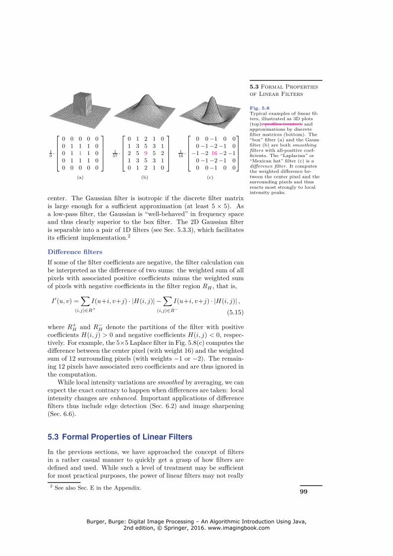
Fig. 5.8
Typical examples of linear fil-ters, illustrated as 3D plots(top), profiles (center), andapproximations by discretefilter matrices (bottom). The“box” filter (a) and the Gaussfilter (b) are both smoothing
filters with all-positive coef-ficients. The “Laplacian” or“Mexican hat” filter (c) is adifference filter. It computesthe weighted difference be-tween the center pixel and thesurrounding pixels and thusreacts most strongly to localintensity peaks.
center. The Gaussian filter is isotropic if the discrete filter matrixis large enough for a sufficient approximation (at least 5 × 5). Asa low-pass filter, the Gaussian is “well-behaved” in frequency spaceand thus clearly superior to the box filter. The 2D Gaussian filteris separable into a pair of 1D filters (see Sec. 5.3.3), which facilitatesits efficient implementation.2
Difference filters
If some of the filter coefficients are negative, the filter calculation canbe interpreted as the difference of two sums: the weighted sum of allpixels with associated positive coefficients minus the weighted sumof pixels with negative coefficients in the filter region RH , that is,
I ′(u, v) =∑
(i,j)∈R+
I(u+i, v+j) · |H(i, j)| −∑
(i,j)∈R−
I(u+i, v+j) · |H(i, j)| ,
(5.15)
where R+H and R−
H denote the partitions of the filter with positivecoefficients H(i, j) > 0 and negative coefficients H(i, j) < 0, respec-tively. For example, the 5×5 Laplace filter in Fig. 5.8(c) computes thedifference between the center pixel (with weight 16) and the weightedsum of 12 surrounding pixels (with weights −1 or −2). The remain-ing 12 pixels have associated zero coefficients and are thus ignored inthe computation.
While local intensity variations are smoothed by averaging, we canexpect the exact contrary to happen when differences are taken: localintensity changes are enhanced. Important applications of differencefilters thus include edge detection (Sec. 6.2) and image sharpening(Sec. 6.6).
5.3 Formal Properties of Linear Filters
In the previous sections, we have approached the concept of filtersin a rather casual manner to quickly get a grasp of how filters aredefined and used. While such a level of treatment may be sufficientfor most practical purposes, the power of linear filters may not really
2 See also Sec. E in the Appendix.99
Burger, Burge: Digital Image Processing – An Algorithmic Introduction Using Java, 2nd edition, © Springer, 2016. www.imagingbook.com

5.3 Formal Properties
of Linear Filters
1
9·
0 0 0 0 00 1 1 1 00 1 1 1 00 1 1 1 00 0 0 0 0
1
57·
0 1 2 1 01 3 5 3 12 5 9 5 21 3 5 3 10 1 2 1 0
1
16·
0 0 −1 0 00 −1 −2 −1 0
−1 −2 16 −2 −10 −1 −2 −1 00 0 −1 0 0
(a) (b) (c)
Fig. 5.8
Typical examples of linear fil-ters, illustrated as 3D plots(top), profiles (center), andapproximations by discretefilter matrices (bottom). The“box” filter (a) and the Gaussfilter (b) are both smoothing
filters with all-positive coef-ficients. The “Laplacian” or“Mexican hat” filter (c) is adifference filter. It computesthe weighted difference be-tween the center pixel and thesurrounding pixels and thusreacts most strongly to localintensity peaks.
center. The Gaussian filter is isotropic if the discrete filter matrixis large enough for a sufficient approximation (at least 5 × 5). Asa low-pass filter, the Gaussian is “well-behaved” in frequency spaceand thus clearly superior to the box filter. The 2D Gaussian filteris separable into a pair of 1D filters (see Sec. 5.3.3), which facilitatesits efficient implementation.2
Difference filters
If some of the filter coefficients are negative, the filter calculation canbe interpreted as the difference of two sums: the weighted sum of allpixels with associated positive coefficients minus the weighted sumof pixels with negative coefficients in the filter region RH , that is,
I ′(u, v) =∑
(i,j)∈R+
I(u+i, v+j) · |H(i, j)| −∑
(i,j)∈R−
I(u+i, v+j) · |H(i, j)| ,
(5.15)
where R+H and R−
H denote the partitions of the filter with positivecoefficients H(i, j) > 0 and negative coefficients H(i, j) < 0, respec-tively. For example, the 5×5 Laplace filter in Fig. 5.8(c) computes thedifference between the center pixel (with weight 16) and the weightedsum of 12 surrounding pixels (with weights −1 or −2). The remain-ing 12 pixels have associated zero coefficients and are thus ignored inthe computation.
While local intensity variations are smoothed by averaging, we canexpect the exact contrary to happen when differences are taken: localintensity changes are enhanced. Important applications of differencefilters thus include edge detection (Sec. 6.2) and image sharpening(Sec. 6.6).
5.3 Formal Properties of Linear Filters
In the previous sections, we have approached the concept of filtersin a rather casual manner to quickly get a grasp of how filters aredefined and used. While such a level of treatment may be sufficientfor most practical purposes, the power of linear filters may not really
2 See also Sec. E in the Appendix.99
Burger, Burge: Digital Image Processing – An Algorithmic Introduction Using Java, 2nd edition, © Springer, 2016. www.imagingbook.com

5 Filters
Fig. 5.7
Border geometry. The filtercan be applied only at lo-
cations where the kernel Hof size (2K + 1) × (2L + 1)
is fully contained in theimage (inner rectangle).
L
L
M
N
KK
H
I
u
v
No coverage
Full coverage
of key importance in practice: smoothing filters and difference filters(Fig. 5.8).
Smoothing filters
Every filter we have discussed so far causes some kind of smoothing.In fact, any linear filter with positive-only coefficients is a smoothingfilter in a sense, because such a filter computes merely a weightedaverage of the image pixels within a certain image region.
Box filter
This simplest of all smoothing filters, whose 3D shape resembles abox (Fig. 5.8(a)), is a well-known friend already. Unfortunately, thebox filter is far from an optimal smoothing filter due to its wild behav-ior in frequency space, which is caused by the sharp cutoff aroundits sides. Described in frequency terms, smoothing corresponds tolow-pass filtering, that is, effectively attenuating all signal compo-nents above a given cutoff frequency (see also Chs. 18–19). The boxfilter, however, produces strong “ringing” in frequency space and istherefore not considered a high-quality smoothing filter. It may alsoappear rather ad hoc to assign the same weight to all image pixels inthe filter region. Instead, one would probably expect to have strongeremphasis given to pixels near the center of the filter than to the moredistant ones. Furthermore, smoothing filters should possibly operate“isotropically” (i.e., uniformly in each direction), which is certainlynot the case for the rectangular box filter.
Gaussian filter
The filter matrix (Fig. 5.8(b)) of this smoothing filter corresponds toa 2D Gaussian function,
HG,σ(x, y) = e− x2+y2
2σ2 = e− r2
2σ2 , (5.14)
where σ denotes the width (standard deviation) of the bell-shapedfunction and r is the distance (radius) from the center. The pixel atthe center receives the maximum weight (1.0, which is scaled to theinteger value 9 in the matrix shown in Fig. 5.8(b)), and the remain-ing coefficients drop off smoothly with increasing distance from the
98
Burger, Burge: Digital Image Processing – An Algorithmic Introduction Using Java, 2nd edition, © Springer, 2016. www.imagingbook.com

12.1 RGB Color Images
RGB
R G B
Fig. 12.2
A color image and its corre-sponding RGB channels. Thefruits depicted are mainly yel-low and red and therefore havehigh values in the R and Gchannels. In these regions, theB content is correspondinglylower (represented here bydarker gray values) except forthe bright highlights on theapple, where the color changesgradually to white. The table-top in the foreground is purpleand therefore displays corre-spondingly higher values in itsB channel.
individual color components. In the next sections we will examinethe difference between true color images, which utilize colors uni-formly selected from the entire color space, and so-called palleted orindexed images, in which only a select set of distinct colors are used.Deciding which type of image to use depends on the requirements ofthe application.
Duplicate text removed.
True color images
A pixel in a true color image can represent any color in its colorspace, as long as it falls within the (discrete) range of its individualcolor components. True color images are appropriate when the im-age contains many colors with subtle differences, as occurs in digitalphotography and photo-realistic computer graphics. Next we look attwo methods of ordering the color components in true color images:component ordering and packed ordering.
293
Burger, Burge: Digital Image Processing – An Algorithmic Introduction Using Java, 2nd edition, © Springer, 2016. www.imagingbook.com

17.2 Bilateral FilterI ′(u, v)←
∞∑
m =−∞
∞∑
n =−∞
I(u + m, v + n) ·Hd(m, n) (17.15)
=
∞∑
i =−∞
∞∑
j =−∞
I(i, j) ·Hd(i− u, j − v), (17.16)
every new pixel value I ′(u, v) is the weighted average of the originalimage pixels I in a certain neighborhood, with the weights specifiedby the elements of the filter kernel Hd.5 The weight assigned toeach pixel only depends on its spatial position relative to the currentcenter coordinate (u, v). In particular, Hd(0, 0) specifies the weightof the center pixel I(u, v), and Hd(m, n) is the weight assigned toa pixel displaced by (m, n) from the center. Since only the spatialimage coordinates are relevant, such a filter is called a domain filter.Obviously, ordinary filters as we know them are all domain filters.
17.2.2 Range Filter
Although the idea may appear strange at first, one could also applya linear filter to the pixel values or range of an image in the form
I ′r(u, v)←
∞∑
i =−∞
∞∑
j =−∞
I(i, j) ·Hr
(I(i, j)− I(u, v)
). (17.17)
The contribution of each pixel is specified by the function Hr anddepends on the difference between its own value I(i, j) and the valueat the current center pixel I(u, v). The operation in Eqn. (17.17)is called a range filter, where the spatial position of a contributingpixel is irrelevant and only the difference in values is considered. Fora given position (u, v), all surrounding image pixels I(i, j) with thesame value contribute equally to the result I ′
r(u, v). Consequently,the application of a range filter has no spatial effect upon the image—in contrast to a domain filter, no blurring or sharpening will occur.Instead, a range filter effectively performs a global point operation byremapping the intensity or color values. However, a global range filter
by itself is of little use, since it combines pixels from the entire imageand only changes the intensity or color map of the image, equivalentto a nonlinear, image-dependent point operation.
17.2.3 Bilateral Filter—General Idea
The key idea behind the bilateral filter is to combine domain filtering(Eqn. (17.16)) and range filtering (Eqn. (17.17)) in the form
I ′(u, v) =1
Wu,v
·
∞∑
i =−∞
∞∑
j =−∞
I(i, j) ·Hd(i−u, j−v) ·Hr
(I(i, j)−I(u, v)
)
︸ ︷︷ ︸wi,j
,
(17.18)
5 In Eqn. (17.16), functions I and Hd are assumed to be zero outside theirdomains of definition.
421
Burger, Burge: Digital Image Processing – An Algorithmic Introduction Using Java, 2nd edition, © Springer, 2016. www.imagingbook.com
17.3 Anisotropic
Diffusion Filters
n = 0 n = 5 n = 10 n = 20 n = 40 n = 80
σn ≈1.411 σn ≈1.996 σn ≈2.823 σn ≈3.992 σn ≈5.646
(a) (b) (c) (d) (e) (f)
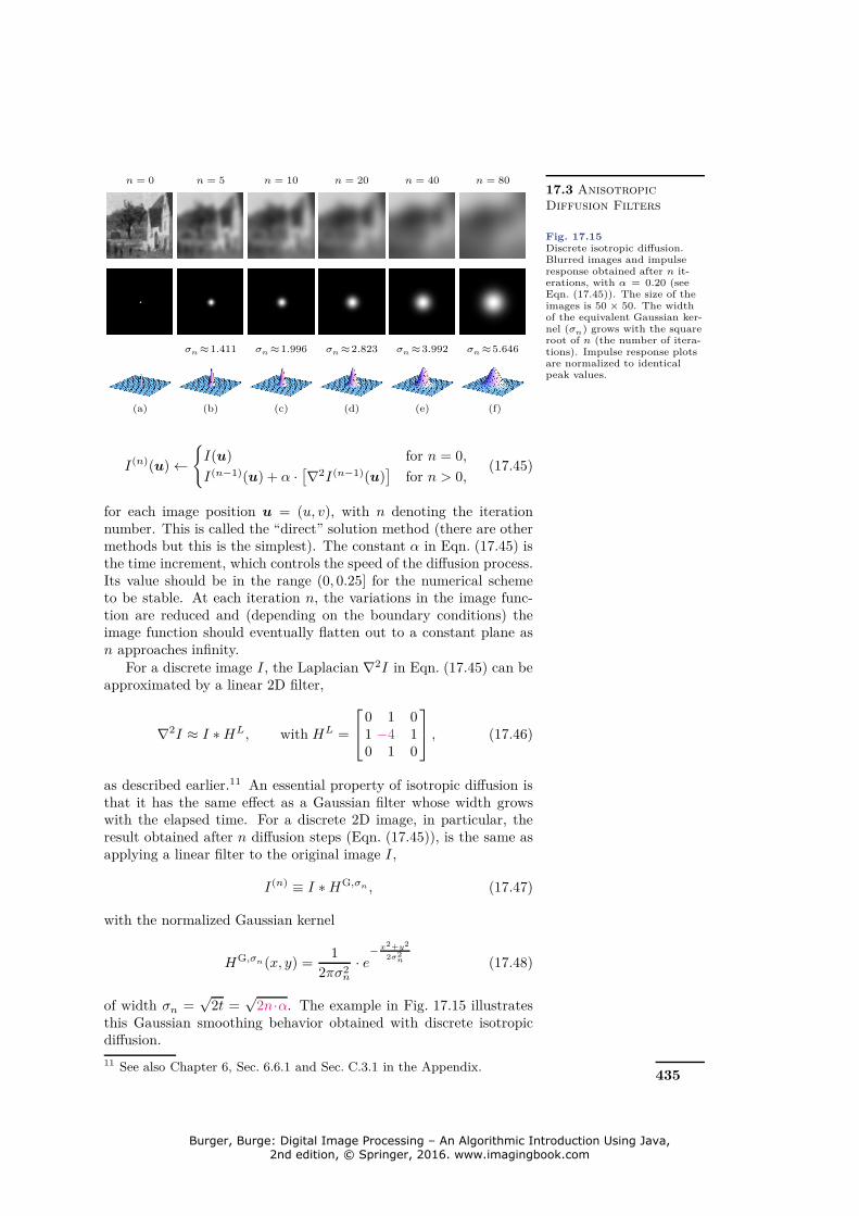
Fig. 17.15
Discrete isotropic diffusion.Blurred images and impulseresponse obtained after n it-erations, with α = 0.20 (seeEqn. (17.45)). The size of theimages is 50 × 50. The widthof the equivalent Gaussian ker-nel (σn) grows with the squareroot of n (the number of itera-tions). Impulse response plotsare normalized to identicalpeak values.
I(n)(u)←
{
I(u) for n = 0,
I(n−1)(u) + α ·[∇2I(n−1)(u)
]for n > 0,
(17.45)
for each image position u = (u, v), with n denoting the iterationnumber. This is called the “direct” solution method (there are othermethods but this is the simplest). The constant α in Eqn. (17.45) isthe time increment, which controls the speed of the diffusion process.Its value should be in the range (0, 0.25] for the numerical schemeto be stable. At each iteration n, the variations in the image func-tion are reduced and (depending on the boundary conditions) theimage function should eventually flatten out to a constant plane asn approaches infinity.
For a discrete image I, the Laplacian ∇2I in Eqn. (17.45) can beapproximated by a linear 2D filter,
∇2I ≈ I ∗HL, with HL =
0 1 01 −4 10 1 0
, (17.46)
as described earlier.11 An essential property of isotropic diffusion isthat it has the same effect as a Gaussian filter whose width growswith the elapsed time. For a discrete 2D image, in particular, theresult obtained after n diffusion steps (Eqn. (17.45)), is the same asapplying a linear filter to the original image I,
I(n) ≡ I ∗HG,σn , (17.47)
with the normalized Gaussian kernel
HG,σn(x, y) =1
2πσ2n
· e− x2+y2
2σ2n (17.48)
of width σn =√
2t =√
2n·α. The example in Fig. 17.15 illustratesthis Gaussian smoothing behavior obtained with discrete isotropicdiffusion.
11 See also Chapter 6, Sec. 6.6.1 and Sec. C.3.1 in the Appendix.435
Burger, Burge: Digital Image Processing – An Algorithmic Introduction Using Java, 2nd edition, © Springer, 2016. www.imagingbook.com

21 Geometric
Operations
Fig. 21.2
Affine mapping. An affine 2Dtransformation is uniquely
specified by three pairsof corresponding points;
for example, (x0, x′
0),(x1, x
′
1), and (x2, x′
2).
I I′
x0
x1
x2
x′
0
x′
1
x′
2
six transformation parameters a00, . . . , a12 are derived by solving thesystem of linear equations
x′0 = a00 ·x0 + a01 ·y0 + a02, y′
0 = a10 ·x0 + a11 ·y0 + a12,
x′1 = a00 ·x1 + a01 ·y1 + a02, y′
1 = a10 ·x1 + a11 ·y1 + a12, (21.25)
x′2 = a00 ·x2 + a01 ·y2 + a02, y′
2 = a10 ·x2 + a11 ·y2 + a12,
provided that the points (vectors) x0, x1, x2 are linearly independent(i.e., that they do not lie on a common straight line). Since Eqn.(21.25) consists of two independent sets of linear 3× 3 equations forx′
i and y′i, the solution can be written in closed form as
a00 = 1d ·[y0(x′
1−x′2) + y1(x′
2−x′0) + y2(x′
0−x′1)],
a01 = 1d ·[x0(x′
2−x′1) + x1(x′
0−x′2) + x2(x′
1−x′0)],
a10 = 1d ·[y0(y′
1−y′2) + y1(y′
2−y′0) + y2(y′
0−y′1)],
a11 = 1d ·[x0(y′
2−y′1) + x1(y′
0−y′2) + x2(y′
1−y′0)],
a02 = 1d ·[x0(y2x′
1−y1x′2) + x1(y0x′
2−y2x′0) + x2(y1x′
0−y0x′1)],
a12 = 1d ·[x0(y2y′
1−y1y′2) + x1(y0y′
2−y2y′0) + x2(y1y′
0−y0y′1)],
(21.26)
with d = x0(y2−y1) + x1(y0−y2) + x2(y1−y0).
Inverse affine mapping
The inverse of the affine transformation, which is often required inpractice (see Sec. 21.2.2), can be calculated by simply applying theinverse of the transformation matrix Aaffine (Eqn. (21.20)) in homo-geneous coordinate space, that is,
x = A−1affine · x
′ (21.27)
or x = hom−1[A−1
affine · hom(x′)]
in Cartesian coordinates, that is,518
Burger, Burge: Digital Image Processing – An Algorithmic Introduction Using Java, 2nd edition, © Springer, 2016. www.imagingbook.com