diffusive gradients in thin-films
DESCRIPTION
Uploaded from Google DocsTRANSCRIPT

Diffusive Gradients in Thin-films (DGT)
March 2002
A Technique for DeterminingBioavailable Metal Concentrations
International Network for Acid Preventi
Part I
DGT Theory and Application Literature Survey

International Network for Acid Preventi
Executive Summary
i
Executive Summary
Trace metals exist in a variety of inorganic and organic forms in aquatic systems,
ranging from simple hydrated molecules to large organic complexes. The biological
availability, and hence toxicity, of metals in aquatic systems is strongly dependent on
the nature of the metal species present. Accordingly, determining the chemical form, or
speciation, of metals in the environment is fundamental to predicting impacts to aquatic
biota.
The presently accepted Free-Ion Activity Model (FIAM) stipulates that the biological
response of organisms to trace metals in waters is proportional to the free-ion activity of
the metals and not their total or dissolved concentrations. This model is predicated on
laboratory experiments with synthetic ligands and not natural organic matter and should
therefore be applied with caution. The model nevertheless properly reflects the fact that
the transport of metals across the biological membrane is the rate-limiting step in the
overall toxic response –– free metal ions (e.g., Cu2+
) are readily taken up by aquatic
organisms, whereas particulate and strongly complexed metals are not. Complexation
of metals in aquatic systems may occur via reaction with soluble inorganic (e.g., F-, Cl
-,
HCO3-, SO4
2-, HPO4
2-, etc.) and organic (e.g., humic substances) ligands. In most
cases, complexation with organic ligands reduces metal bioavailability, because most
organic-metal complexes are not readily transported across cell membranes. Inorganic-
metal complexes (e.g., carbonates), however, typically dissociate rapidly to the free
metal form. Thus, while the bioavailable fraction of metals includes both free metal
ions and kinetically–labile metal complexes (i.e., those with rapid dissociation kinetics),
the biological response is proportional to the free-metal concentration only.
A variety of metal species have been identified in natural waters, including both
inorganic and organic species. The relative proportions of the various species depend
on the concentrations of the metals present, the specific characteristics of the water (i.e.,
ionic strength and pH), and on the concentrations and strengths of the various ligands
present. In addition, the metallurgical processing of base metal and gold ores involves
the addition of various reagents (which may act as ligands) to enhance the recovery of
desirable constituents. As a result, ligands present in mining-related discharges may
contrast greatly from those present in natural waters, which in turn could have a
profound effect on metal speciation and toxicity in the receiving environment.
Recognizing the limitations of conventional methods for estimating water quality,
which are typically restricted to partitioning metals between total and “dissolved”
phases, a variety of analytical and test methods have been used to quantify metal
EXECUTIVE SUMMARY PART I: DGT THEORY AND APPLICATION ii
INAP LORAX
toxicity and speciation in natural waters and effluents. Virtually all of the techniques
suffer inadequacies that limit their general use. For example, most existing speciation
and toxicity techniques must be carried out in a laboratory, rather than in situ, resulting
in the potential for changes in metal speciation and therefore toxicity. Further,
electrochemical in situ speciation techniques require expensive instrumentation that
must be used by highly trained operators, making such techniques onerous and non-
routine.
DGT represents a relatively new approach for in situ determinations of labile metal-
species in aquatic systems. The DGT device passively accumulates labile species from
solution while deployed in situ and therefore contamination problems associated with
conventional water collection and filtration procedures are eliminated. Since DGT
affords an operationally defined measure of the labile, or "bioavailable" fraction,
inferences can be made with respect to metal toxicity.
The theory behind DGT is based on the diffusional characteristics of metals in a
hydrogel and on the ion exchange properties of a metal-binding resin. Specifically, the
technique utilizes a hydrogel layer to control the diffusive transport of metals in
solution to a cation-exchange resin. In addition, since the resin used in DGT (Chelex)
is selective for free or weakly complexed species, it provides a proxy for the labile
fraction of metals in solution.
DGT utilizes a three-layer system consisting of: 1) a resin-impregnated hydrogel layer;
2) a hydrogel diffusion-layer; and 3) a filter membrane. The innermost two gel layers
are fabricated from a polyacrylamide hydrogel. The filter membrane isolates the
polyacrylamide surface from particles in the water. Labile metal ions in solution diffuse
across the filter and gel layers and are pre-concentrated on the resin. Based on the laws
of diffusion and the established characteristics of the diffusive path in the DGT
sampler, the concentration of labile metals in solution may be calculated using the
measured metal ion inventory on the resin, the sampler exposure time and the
temperature-corrected molecular diffusion coefficient for the metal of interest. A
qualification of the method is that the calculated labile-metal concentration depends on
the diffusion coefficient D adopted for the hydrogel. Ionic strength, pH, and solution
composition can influence the rate of diffusion, for example by affecting the behaviour
of functional groups on the polyacrylamide, which may become ionized. Although
some workers have assumed that diffusion coefficients in the gels are similar to those in
water, this overstates the case because tortuosity and permeability effects lower the rate
of diffusion. Such effects become more pronounced as the gel becomes tighter. These
effects have been compensated for through the direct measurement of diffusion
coefficients within the hydrogel.
EXECUTIVE SUMMARY PART I: DGT THEORY AND APPLICATION iii
INAP LORAX
Waters with very low cation concentrations (<2 x 10⁻⁴
M) also pose a potential
challenge. In such settings, the sodium form of polyacrylamide used in the gel samplers
can establish negative concentration gradients of Na+ from the gel to the sample water.
To preserve electro neutrality, the charge imbalance is compensated by steepened
concentration gradients of cations in the opposite direction. These enhance the flux of
cations to the gel, causing their "labile" concentrations to be overestimated. In most
mining-impacted regions, this is not of importance because surface waters typically
have higher ionic strengths. But in pristine natural waters with low ionic strength, for
example, this co-diffusion effect may be important. The three-layered DGT
configuration is held within a plastic holder (4 cm diameter disc). Hydrated DGT
samplers are stored refrigerated in sealed plastic bags until immediately before
deployment. Deployment typically involves suspension of the device in situ or in a
stirred solution in the laboratory for a period typically ranging between one and twenty-
four hours (depending on metal concentrations in the test solution). Deployment
duration and temperature are recorded during deployment. Upon retrieval, the DGT
units are rinsed with distilled deionized water and refrigerated in sealed plastic bags to
avoid dehydration and potential contamination. The samplers are disassembled and the
resin layer analyzed for metal content, by either analysis of an acid extract (e.g., by ICP-
MS) or through direct analysis of the resin beads by techniques such as proton induced
X-ray emission (PIXE) or laser ablation.
An important consideration with respect to the interpretation of DGT data is that the
methodology integrates the concentration of labile metals in solution over the
deployment period. Under conditions where variability in water quality is low, DGT
data are comparable to more conventional sampling approaches, which are more
instantaneous in nature. If, however, an aquatic system hosts some degree of variability
(such as is often the case where effluents are discharged into a natural water course),
then grab samples for water quality assessment may not be directly comparable to the
time-integrated metal signature determined by DGT.
Between any solid and a liquid there is a zone of laminar flow in which the process of
molecular diffusion dominates solute transport. This zone (which typically ranges in
thickness between 0.1 and 1 mm, depending on the interfacial flow velocity) is referred
to as the diffusive boundary layer (DBL). The presence of the DBL between the DGT
sampler and the bulk solution serves to increase the diffusive path-length over which
ions must travel in order to be fixed by the DGT sampler. The thickness of the DBL
under conditions of flow is sufficiently small such that impacts on metal uptake are
negligible. However, as flow diminishes, the DBL thickens and multiple samplers of
differing gel-layer thicknesses must be deployed in order to derive a DBL correction
factor.
EXECUTIVE SUMMARY PART I: DGT THEORY AND APPLICATION iv
INAP LORAX
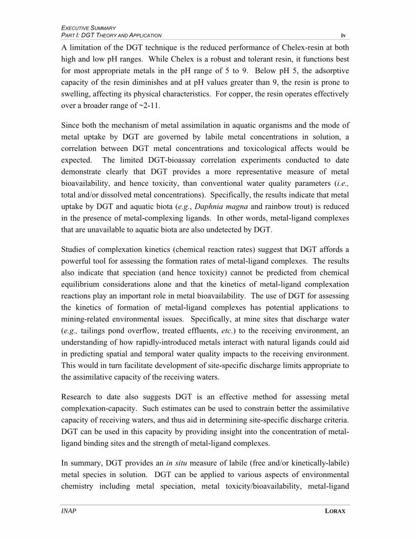
A limitation of the DGT technique is the reduced performance of Chelex-resin at both
high and low pH ranges. While Chelex is a robust and tolerant resin, it functions best
for most appropriate metals in the pH range of 5 to 9. Below pH 5, the adsorptive
capacity of the resin diminishes and at pH values greater than 9, the resin is prone to
swelling, affecting its physical characteristics. For copper, the resin operates effectively
over a broader range of ~2-11.
Since both the mechanism of metal assimilation in aquatic organisms and the mode of
metal uptake by DGT are governed by labile metal concentrations in solution, a
correlation between DGT metal concentrations and toxicological affects would be
expected. The limited DGT-bioassay correlation experiments conducted to date
demonstrate clearly that DGT provides a more representative measure of metal
bioavailability, and hence toxicity, than conventional water quality parameters (i.e.,
total and/or dissolved metal concentrations). Specifically, the results indicate that metal
uptake by DGT and aquatic biota (e.g., Daphnia magna and rainbow trout) is reduced
in the presence of metal-complexing ligands. In other words, metal-ligand complexes
that are unavailable to aquatic biota are also undetected by DGT.
Studies of complexation kinetics (chemical reaction rates) suggest that DGT affords a
powerful tool for assessing the formation rates of metal-ligand complexes. The results
also indicate that speciation (and hence toxicity) cannot be predicted from chemical
equilibrium considerations alone and that the kinetics of metal-ligand complexation
reactions play an important role in metal bioavailability. The use of DGT for assessing
the kinetics of formation of metal-ligand complexes has potential applications to
mining-related environmental issues. Specifically, at mine sites that discharge water
(e.g., tailings pond overflow, treated effluents, etc.) to the receiving environment, an
understanding of how rapidly-introduced metals interact with natural ligands could aid
in predicting spatial and temporal water quality impacts to the receiving environment.
This would in turn facilitate development of site-specific discharge limits appropriate to
the assimilative capacity of the receiving waters.
Research to date also suggests DGT is an effective method for assessing metal
complexation-capacity. Such estimates can be used to constrain better the assimilative
capacity of receiving waters, and thus aid in determining site-specific discharge criteria.
DGT can be used in this capacity by providing insight into the concentration of metal-
ligand binding sites and the strength of metal-ligand complexes.
In summary, DGT provides an in situ measure of labile (free and/or kinetically-labile)
metal species in solution. DGT can be applied to various aspects of environmental
chemistry including metal speciation, metal toxicity/bioavailability, metal-ligand
EXECUTIVE SUMMARY PART I: DGT THEORY AND APPLICATION v
INAP LORAX
complexation kinetics and metal complexation-capacity. Given its range of application,
ease of use and relatively low cost, DGT has the potential to become a routine water
quality monitoring tool in studies of mining-impacted systems. In particular, DGT-
inferred values may compliment standard metal measurements (e.g., total and dissolved
metals), while affording site-specific information with respect to metal toxicity.
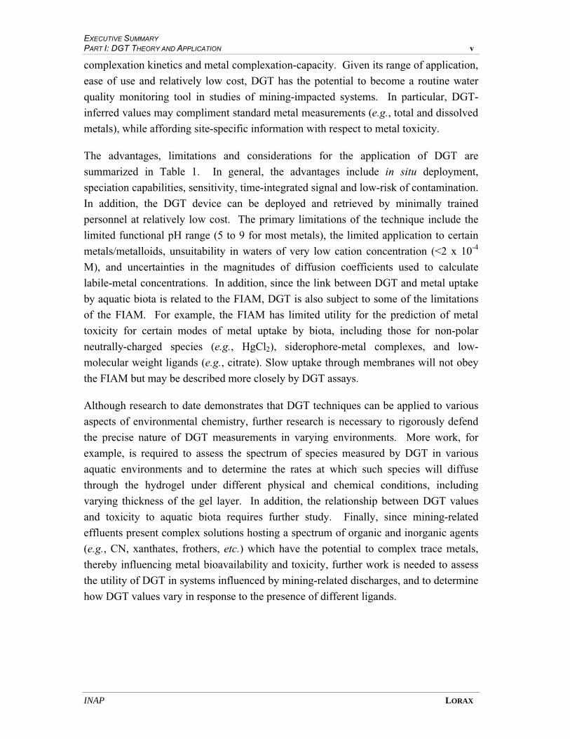
The advantages, limitations and considerations for the application of DGT are
summarized in Table 1. In general, the advantages include in situ deployment,
speciation capabilities, sensitivity, time-integrated signal and low-risk of contamination.
In addition, the DGT device can be deployed and retrieved by minimally trained
personnel at relatively low cost. The primary limitations of the technique include the
limited functional pH range (5 to 9 for most metals), the limited application to certain
metals/metalloids, unsuitability in waters of very low cation concentration (<2 x 10⁻⁴
M), and uncertainties in the magnitudes of diffusion coefficients used to calculate
labile-metal concentrations. In addition, since the link between DGT and metal uptake
by aquatic biota is related to the FIAM, DGT is also subject to some of the limitations
of the FIAM. For example, the FIAM has limited utility for the prediction of metal
toxicity for certain modes of metal uptake by biota, including those for non-polar
neutrally-charged species (e.g., HgCl2), siderophore-metal complexes, and low-
molecular weight ligands (e.g., citrate). Slow uptake through membranes will not obey
the FIAM but may be described more closely by DGT assays.
Although research to date demonstrates that DGT techniques can be applied to various
aspects of environmental chemistry, further research is necessary to rigorously defend
the precise nature of DGT measurements in varying environments. More work, for
example, is required to assess the spectrum of species measured by DGT in various
aquatic environments and to determine the rates at which such species will diffuse
through the hydrogel under different physical and chemical conditions, including
varying thickness of the gel layer. In addition, the relationship between DGT values
and toxicity to aquatic biota requires further study. Finally, since mining-related
effluents present complex solutions hosting a spectrum of organic and inorganic agents
(e.g., CN, xanthates, frothers, etc.) which have the potential to complex trace metals,
thereby influencing metal bioavailability and toxicity, further work is needed to assess
the utility of DGT in systems influenced by mining-related discharges, and to determine
how DGT values vary in response to the presence of different ligands.

EXECUTIVE SUMMARY PART I: DGT THEORY AND APPLICATION vi
INAP LORAX
Table 1: Summary of the advantages, limitations and considerations
associated with the use of DGT in aquatic systems
Advantages Limitations/Considerations
Speciation: provides an in situ measure of labile metal species in solution. Allows inference of metal bioavailability and toxicity.
pH: limited pH range of Chelex resin (pH 5 to 9, but ~2-11 for Cu)
Accuracy of assayed concentrations depends on knowledge of diffusion coefficients in hydrogel. These may not be rigourously known.
Co diffusion can be a constraint in waters of very low cation concentrations (<2 x 10⁻⁴ M)
Sensitivity: pre-concentration of metals allows for ultra trace-level determinations.
Capabilities have not been rigourously defined for some metals/metalloids (e.g., Mo, As, Se)
Contamination: the potential for contamination associated with water collection and filtration is eliminated.
FIAM: subject to some of the limitations of
the free-ion activity model.
Analytical Interferences: obviates matrix effects associated with conventional analyses of high ionic-strength solutions.
Metal Species Detected: requires more precise determination of the spectrum of species detected (e.g., kinetically-labile).
Time Integration: provides a time-integrated measure of labile-metal species over desired deployment interval.
Mining-Impacted Systems: more work is required to validate the use of DGT in mining-impacted environments.
Multitude of Applications:
• Metal speciation
• Toxicity testing
• Complexation kinetics of metal-ligand complexes
• Complexation Capacity
• Development of site-specific discharge criteria and assimilative capacity
DGT vs. toxicity: additional study is required assess the relationship between DGT values and toxicity to aquatic biota.
User Friendly: deployment and retrieval do not require specialized equipment or highly trained personnel.
Costs: costs are compatible with standard water quality analyses.

International Network for Acid Preventi
Table of Contents
vii
Table of Contents
EXECUTIVE SUMMARY ...................................................................................................................... i
1 INTRODUCTION ............................................................................................................................. 1-1
2 METAL TOXICITY.........................................................................................................................2-1 2.1 INTRODUCTION...................................................................................................................... 2-1
2.2 NATURE OF TOXICITY ........................................................................................................... 2-1
2.3 UPTAKE MECHANISMS .......................................................................................................... 2-2
2.3 MITIGATING FACTORS ........................................................................................................... 2-5
2.5 FREE-ION ACTIVITY MODEL.................................................................................................. 2-6
2.6 ASSESSMENT TECHNIQUES.................................................................................................... 2-7
3 METAL SPECIATION ..................................................................................................................... 3-1 3.1 INTRODUCTION...................................................................................................................... 3-1
3.2 SPECIATION IN NATURAL WATERS ........................................................................................ 3-1
3.2.1 “DISSOLVED” METALS ............................................................................................... 3-2
3.2.1.1 INORGANIC SPECIES ..................................................................................... 3-2
3.2.1.2 ORGANIC SPECIES ........................................................................................ 3-2
3.2.1.3 EFFECTS OF LIGAND CONCENTRATION AND STRENGTH ON SPECIATION....... 3-3
3.2.1.4 CASE STUDIES OF SPECIATION IN NATURAL WATERS................................... 3-5
3.2.2 PARTICULATE METAL SPECIES ................................................................................... 3-6
3.3 METAL SPECIATION IN MINING-IMPACTED SYSTEMS ............................................................ 3-7
3.4 SPECIATION TECHNIQUES...................................................................................................... 3-9
3.4.1 DGT........................................................................................................................... 3-9
3.4.2 VOLTAMMETRY (ASV AND ADCSV) ......................................................................... 3-10
3.4.3 SUPPORTED LIQUID MEMBRANE................................................................................. 3-11
3.4.4 OTHER........................................................................................................................ 3-13
3.5 SUMMARY............................................................................................................................. 3-13
4 DGT............................................................................................................................................... 4-1 4.1 INTRODUCTION...................................................................................................................... 4-1
4.2 DGT THEORY AND DESIGN................................................................................................... 4-2
4.2.1 DGT THEORY ............................................................................................................ 4-2
4.2.2 CALCULATION OF CONCENTRATION ........................................................................... 4-5
4.2.3 THE DGT SAMPLER ................................................................................................... 4-8
4.3 DGT APPLICATIONS.............................................................................................................. 4-9
4.3.1 THE MEASUREMENT OF SPECIATION AS DETERMINED BY DGT ................................. 4-9
4.3.2 TOXICITY.................................................................................................................... 4-15
4.3.3 KINETICS OF COMPLEXATION ..................................................................................... 4-20
4.3.4 COMPLEXATION CAPACITY......................................................................................... 4-23
4.4 CONSIDERATIONS AND LIMITATIONS ..................................................................................... 4-26
4.5 DATA GAPS AND FUTURE RESEARCH.................................................................................... 4-29
5 DGT SEDIMENT PROBE ...............................................................................................................5-1 5.1 INTRODUCTION...................................................................................................................... 5-1
5.2 EXISTING TECHNIQUES FOR ASSESSING SEDIMENT GEOCHEMISTRY AND TOXICITY.............. 5-1
5.2.1 SEDIMENT/TAILINGS REACTIVITY ASSESSMENT ......................................................... 5-1
5.2.2 TOXICOLOGICAL ASSESSMENT ................................................................................... 5-2
5.3 THEORY AND APPLICATION OF THE DGT SEDIMENT PROBE ................................................. 5-5
5.3.1 DGT SEDIMENT PROBE THEORY AND DESIGN ........................................................... 5-5
5.3.2 DGT SEDIMENT PROBE APPLICATIONS ...................................................................... 5-10
5.4 SUMMARY............................................................................................................................. 5-11
TABLE OF CONTENTS PART I: DGT THEORY AND APPLICATION viii
INAP LORAX
REFERENCES ...................................................................................................................................... R-1
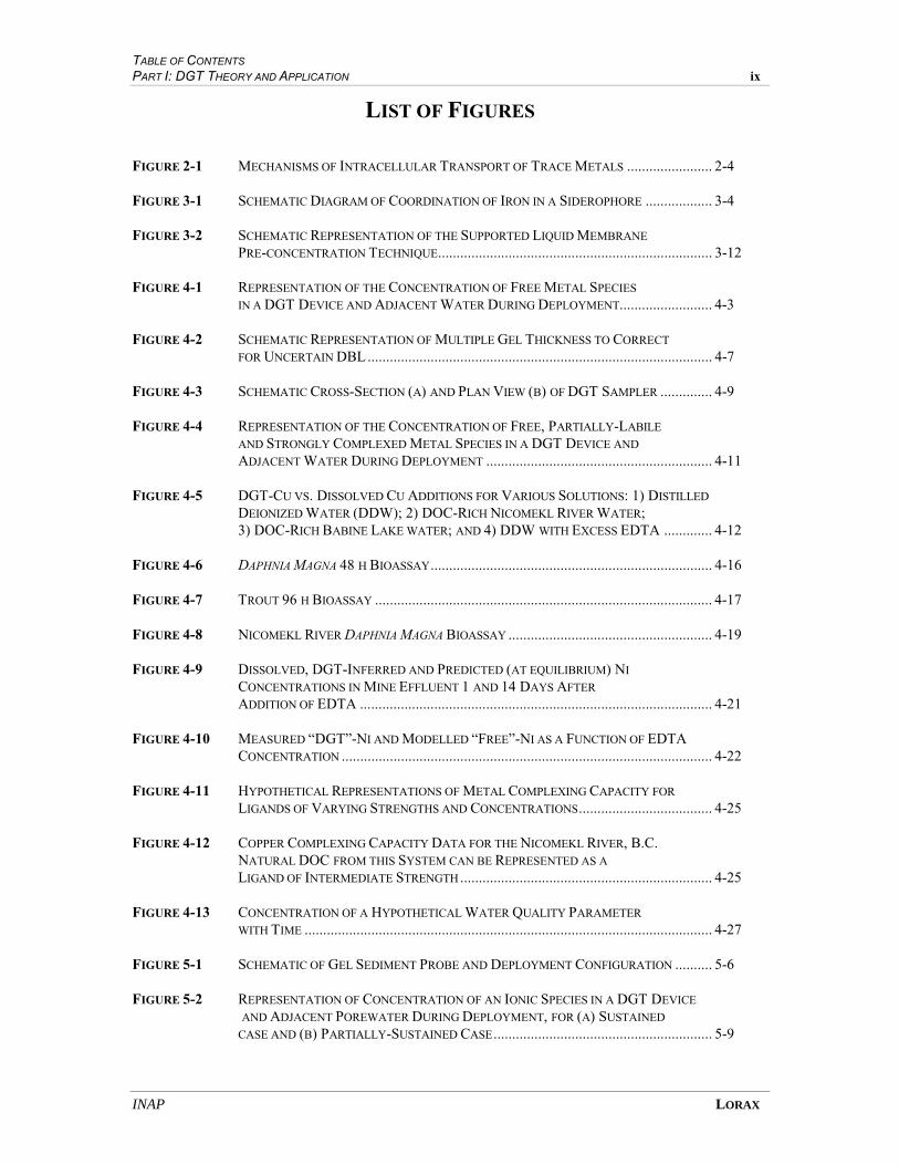
TABLE OF CONTENTS PART I: DGT THEORY AND APPLICATION ix
INAP LORAX
LIST OF FIGURES FIGURE 2-1 MECHANISMS OF INTRACELLULAR TRANSPORT OF TRACE METALS ....................... 2-4
FIGURE 3-1 SCHEMATIC DIAGRAM OF COORDINATION OF IRON IN A SIDEROPHORE .................. 3-4
FIGURE 3-2 SCHEMATIC REPRESENTATION OF THE SUPPORTED LIQUID MEMBRANE
PRE-CONCENTRATION TECHNIQUE.......................................................................... 3-12
FIGURE 4-1 REPRESENTATION OF THE CONCENTRATION OF FREE METAL SPECIES
IN A DGT DEVICE AND ADJACENT WATER DURING DEPLOYMENT......................... 4-3
FIGURE 4-2 SCHEMATIC REPRESENTATION OF MULTIPLE GEL THICKNESS TO CORRECT
FOR UNCERTAIN DBL............................................................................................. 4-7
FIGURE 4-3 SCHEMATIC CROSS-SECTION (A) AND PLAN VIEW (B) OF DGT SAMPLER .............. 4-9
FIGURE 4-4 REPRESENTATION OF THE CONCENTRATION OF FREE, PARTIALLY-LABILE
AND STRONGLY COMPLEXED METAL SPECIES IN A DGT DEVICE AND
ADJACENT WATER DURING DEPLOYMENT ............................................................. 4-11
FIGURE 4-5 DGT-CU VS. DISSOLVED CU ADDITIONS FOR VARIOUS SOLUTIONS: 1) DISTILLED
DEIONIZED WATER (DDW); 2) DOC-RICH NICOMEKL RIVER WATER;
3) DOC-RICH BABINE LAKE WATER; AND 4) DDW WITH EXCESS EDTA ............. 4-12
FIGURE 4-6 DAPHNIA MAGNA 48 H BIOASSAY............................................................................ 4-16
FIGURE 4-7 TROUT 96 H BIOASSAY ........................................................................................... 4-17
FIGURE 4-8 NICOMEKL RIVER DAPHNIA MAGNA BIOASSAY ....................................................... 4-19
FIGURE 4-9 DISSOLVED, DGT-INFERRED AND PREDICTED (AT EQUILIBRIUM) NI
CONCENTRATIONS IN MINE EFFLUENT 1 AND 14 DAYS AFTER
ADDITION OF EDTA ............................................................................................... 4-21
FIGURE 4-10 MEASURED “DGT”-NI AND MODELLED “FREE”-NI AS A FUNCTION OF EDTA
CONCENTRATION .................................................................................................... 4-22
FIGURE 4-11 HYPOTHETICAL REPRESENTATIONS OF METAL COMPLEXING CAPACITY FOR
LIGANDS OF VARYING STRENGTHS AND CONCENTRATIONS.................................... 4-25
FIGURE 4-12 COPPER COMPLEXING CAPACITY DATA FOR THE NICOMEKL RIVER, B.C.
NATURAL DOC FROM THIS SYSTEM CAN BE REPRESENTED AS A
LIGAND OF INTERMEDIATE STRENGTH.................................................................... 4-25
FIGURE 4-13 CONCENTRATION OF A HYPOTHETICAL WATER QUALITY PARAMETER
WITH TIME .............................................................................................................. 4-27
FIGURE 5-1 SCHEMATIC OF GEL SEDIMENT PROBE AND DEPLOYMENT CONFIGURATION .......... 5-6
FIGURE 5-2 REPRESENTATION OF CONCENTRATION OF AN IONIC SPECIES IN A DGT DEVICE
AND ADJACENT POREWATER DURING DEPLOYMENT, FOR (A) SUSTAINED
CASE AND (B) PARTIALLY-SUSTAINED CASE........................................................... 5-9
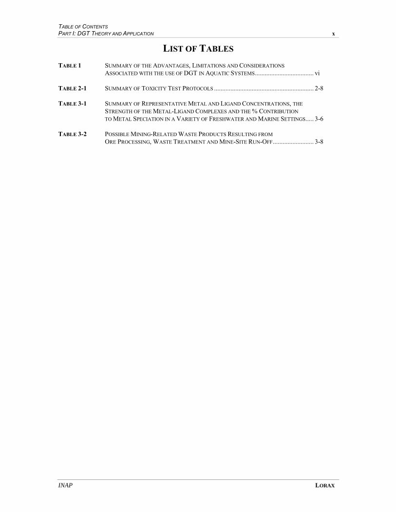
TABLE OF CONTENTS PART I: DGT THEORY AND APPLICATION x
INAP LORAX
LIST OF TABLES TABLE 1 SUMMARY OF THE ADVANTAGES, LIMITATIONS AND CONSIDERATIONS
ASSOCIATED WITH THE USE OF DGT IN AQUATIC SYSTEMS.................................... vi TABLE 2-1 SUMMARY OF TOXICITY TEST PROTOCOLS ............................................................. 2-8
TABLE 3-1 SUMMARY OF REPRESENTATIVE METAL AND LIGAND CONCENTRATIONS, THE
STRENGTH OF THE METAL-LIGAND COMPLEXES AND THE % CONTRIBUTION
TO METAL SPECIATION IN A VARIETY OF FRESHWATER AND MARINE SETTINGS..... 3-6
TABLE 3-2 POSSIBLE MINING-RELATED WASTE PRODUCTS RESULTING FROM
ORE PROCESSING, WASTE TREATMENT AND MINE-SITE RUN-OFF......................... 3-8

International Network for Acid Preventi
1 Introduction

1-1
1. Introduction
The technique of diffusive gradients in thin-film (DGT) has been developed over the past
ten years by academic researchers in order to provide a method for in situ determinations
of “labile” metal species in natural waters. Since it is the labile fraction of the total metal
inventory that is considered most bioavailable to aquatic organisms, DGT has the
potential to become an important tool in toxicological and environmental assessments.
The technique is particularly germane to the needs of the mining industry, given the lack
of appropriate and routine in situ methods for assessing the site-specific toxicity of metal-
contaminated waters.
The International Network for Acid Prevention (INAP) commissioned Lorax
Environmental Services Ltd. (Lorax) to conduct a two-phase study to establish the current
state-of-knowledge of DGT technology (Phase-1) and to conduct further validation work
on DGT (Phase-2). More specifically, phase-one of the study, which is the subject of this
section, consists of a comprehensive literature survey, which reviews the latest
developments in DGT techniques and assesses the applicability of DGT to mining-related
environmental studies. To this end, over 250 papers were reviewed and approximately
200 are cited in Part I of this report.
Under the present regulatory framework, water quality criteria for mine sites are typically
based on total metal concentrations in the receiving environment and/or laboratory
bioassays conducted on mine effluents. The principal weaknesses of these approaches
relate to the fact that total metal concentrations are not a good proxy for metal
bioavailability (i.e., toxicity) and that the handling, transport and processing of water
samples associated with bioassays may result in significant changes in metal speciation,
and therefore toxicity. The limitations of these approaches are described in detail in
Chapters 2 and 3.
DGT represents a relatively new approach to water sampling, which essentially obviates
many of the limitations outlined above. In general, DGT samples labile metal species in
aquatic systems and therefore affords in situ assays of metal speciation. Accordingly, the
technique allows inferences to bioavailability and toxicity. The DGT approach also
obviates contamination problems associated with water collection and filtration. To date,
DGT has been successfully used to estimate concentrations of labile species of iron,
manganese, cadmium, cobalt, copper, nickel, lead and zinc. However, additional
validation/verification work is required to advance the DGT sampler as a reliable in situ
toxicity indicator for routine use by the mining industry.
INTRODUCTION PART I: DGT THEORY AND APPLICATION 1-2
INAP LORAX
The inclusion of metal toxicity (Chapter 2) and speciation (Chapter 3) in this review was
necessary to define the mechanisms of metal assimilation by aquatic biota, and to relate
these processes to metal uptake via DGT. A comprehensive review of the DGT technique
is presented in Chapter 4. This includes a detailed description of the theory and design of
the DGT water sampler, a discussion of DGT applications, and a summary of the current
considerations and limitations. Academic researchers have also developed a DGT pore
water sampler that has considerable potential as a tool for assessing the subaqueous
reactivity of tailings and contaminated sediments, as well as for providing a measure of
sediment toxicity. Although a full assessment of the DGT pore water sampler or
“sediment probe” is outside the scope of the present INAP study, the details of its
function and application are provided for completeness (Chapter 5).

International Network for Acid Preventi
2 Metal Toxicity
2-1
2. Metal Toxicity
2.1 Introduction
Many trace metals are micronutrients and represent essential dietary components of
aquatic organisms. Such "nutrient" metals include Fe, Cu, Zn, Ni, Mn, Co, Cd, Mo, Se,
Sn, and V (Florence, 1982). In natural marine environments and freshwaters, most trace
elements are typically present in trace quantities (<10 nM) and are passively and/or
actively assimilated by organisms to satisfy physiological requirements. In metal-
contaminated systems, however, metals can accumulate within the cells and tissues of
organisms, which could result in effects deleterious to cellular function. Indeed, varying
"toxic" responses, ranging from impaired metabolism to death have been observed for
most metals, including the micronutrient elements outlined above.
In the following sections, metal toxicity is first described with respect to the nature of
metal-induced physiological impairment (Section 2.2). Subsequent to a discussion of the
processes governing the metal uptake by cells (Section 2.3), factors which ameliorate
metal toxicity are described (Section 2.3). The background outlined in the latter sections
forms the foundation for discussion of the Free-Ion Activity Model (FIAM) (Section 2.5).
The FIAM is based on the positive relationship between bioavailability (i.e., toxicity) and
the concentration of the free metal-ion, and provides the link between toxicity and DGT-
derived metal concentrations. The chapter concludes with a brief review of the current
methodologies for toxicity testing (Section 2.6).
2.2 Nature of Toxicity
The bioavailability and toxicity of metals to aquatic biota have been examined
extensively using a variety of test organisms including phytoplankton (Sunda and
Guillard, 1976; Anderson and Morel, 1979; Fisher, 1986; Phinney and Bruland, 1997;
Errécalde et al., 1998; Sunda and Huntzman, 1992; Errécalde and Campbell, 2000;
Franklin et al., 2000), bivales (Zamuda et al., 1985; Tessier et al., 1993; Absil et al.,
1994; Wang and Fisher, 1996), crustaceans (LaPorte et al., 1997; Barata et al., 1998;
Reinfelder et al., 1998; Baillieul and Blust, 1999; Carvalho et al., 1999; Wang and
Fisher, 1999a; Soegianto et al., 1999; Rainbow et al., 2000), fish (Spry and Winer, 1991;
Wilkenson et al., 1993; Roy and Campbell, 1995; Hollis et al., 1996; Playle, 1998; Meyer
et al., 1999) and aquatic insects (Craig et al., 1999; Bervoets and Blust, 1999, 2000). The
effects of metal toxicity are variable, but are generally expressed as mortality, decreased
growth rate, decreased fecundity and decreased metabolic activity. Metals are toxic
because in sufficient concentrations they are able to compete for intracellular sites
METAL TOXICITY PART I: DGT THEORY AND APPLICATION 2-2
INAP LORAX
normally occupied by functional metabolites, thereby interfering with normal cell
functions. Metal coordination sites are rarely entirely specific for a single metal, and
therefore surface sites designed to bind nutrient metals will also bind non-essential (and
potentially toxic) metals with similar ionic radii and coordination geometry. Cu, Zn and
Cd, for example, have been shown to compete for Mn uptake sites (Sunda and Huntzman,
1998). Once inside the cell, competing metals can bind to nutrient-metal coordination
sites such as metabolic sites on metalloproteins, resulting in a loss of metabolic function
and inhibition of cellular function.
2.3 Uptake Mechanisms
The accumulation of metals in organisms can occur via uptake of metals in food sources
and/or exposure to metals in the surrounding medium (Hare and Tessier, 1996; Wang and
Fisher, 1999a, b). Sources of food-bound metals may include phytoplankton, detritus,
and inorganic particles (e.g., suspended solids and sediments). Indeed, for many aquatic
invertebrates, the trophic transfer of metals from prey to predator accounts for a major
portion of the total metal accumulation (Reinfelder et al., 1998). In general, the nature of
metal assimilation from food particles is complex, being influenced by a number of
abiotic (e.g., temperature, pH) and biological (e.g., ingestion rate, gut volume/gut passage
time, digestive enzyme activity and metal partitioning) factors. A more detailed
description of sediment toxicity is provided in Chapter 5.
Metals may also be assimilated via contact/ingestion of water and sediment pore waters.
For example, waterborne metals can be biologically assimilated via binding to the gills of
fish, bivalves and crustaceans (e.g., Wilkinson, et al., 1993; Hollis et al., 1996; Playle,
1998; Soegianto, et al., 1999), across digestive membranes (Reinfelder et al., 1998) and
via direct uptake across the cell membranes of unicellular organisms (Anderson and
Morel, 1979).
The regulation of materials into and out of a cell is facilitated by the cell membrane,
which simply termed, is composed of phospholipids and large protein molecules.
Phospholipid molecules are arranged in a bilayer in which nonpolar (i.e., hydrophobic)
fatty acids are sandwiched between polar (hydrophilic) phosphate groups. Globular
proteins (integral proteins) are dispersed throughout the lipid bilayer, and act as conduits
for the transport of materials to the cell interior.
Most metal species are extremely hydrophilic, and as a result, their passage through the
hydrophobic lipid membrane is restricted. Dissolved metals are typically incorporated
passively into the cells of organisms via specialized pumps, channels and carriers which
operate across the membrane surface. Pump and channel metal-transporters comprise
METAL TOXICITY PART I: DGT THEORY AND APPLICATION 2-3
INAP LORAX
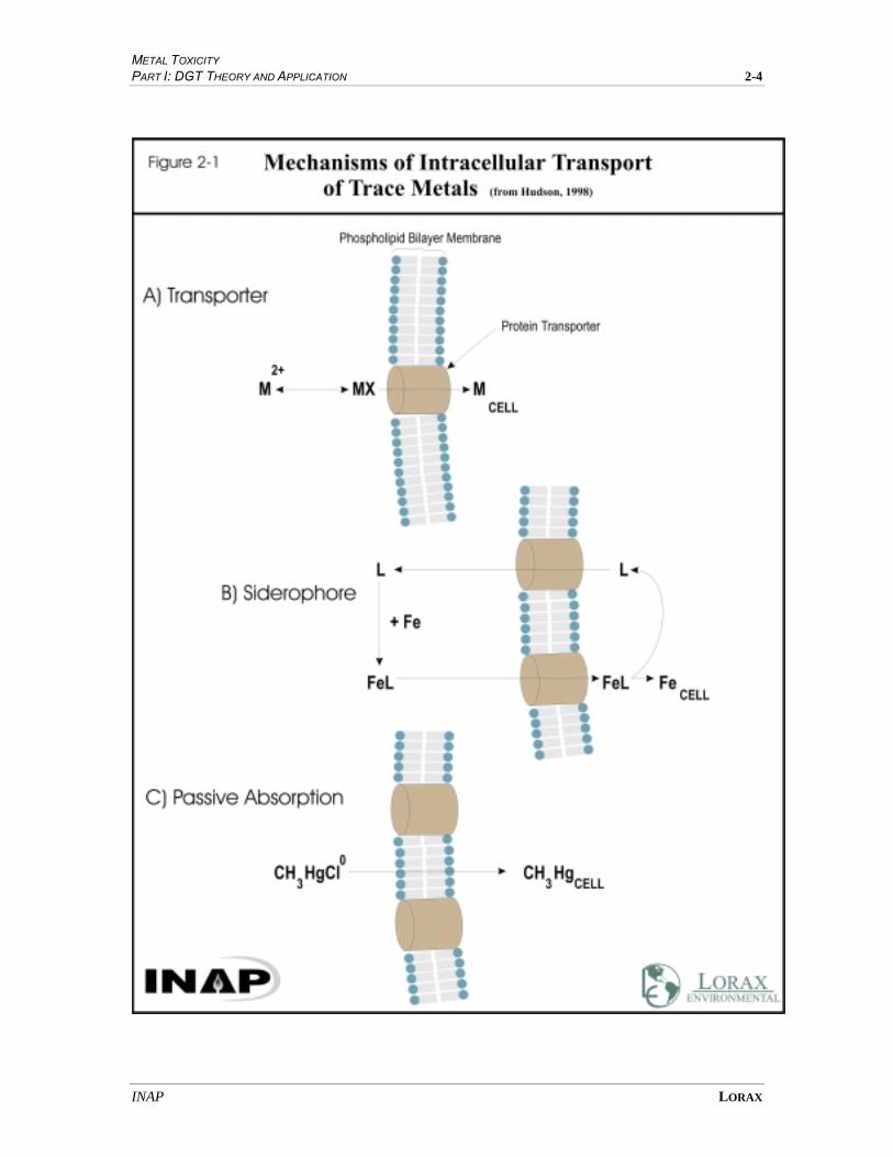
membrane proteins that facilitate metal transport across the cell membrane (Figure 2-1).
Metal ions bind to receptor sites on the protein, and are subsequently transported across
the membrane and released into the cytoplasm of the cell. Conversely, carriers represent
lipid-soluble molecules that bind metals on the cell exterior, diffuse across the membrane
and transfer the metal complex to the cell interior.
Metal transport across cellular membranes may also be facilitated via extracellular
chelators. Aquatic prokaryotes, for example, release high-affinity Fe chelators, or
siderophores, into the environment when they become iron-limited (Wilhelm and Trick,
1994). Siderophores complex Fe at the cell surface, with the resulting Fe-chelator
complex being transported by membrane receptors into the cell cytoplasm (Figure 2-1).
The Fe is subsequently remobilized and incorporated into the cell. A detailed discussion
of siderophore structure and function is presented in Chapter 3. Similar strategies have
been demonstrated for phytoplanktons which have been observed to produce extracellular
Cu complexing ligands in respond to Cu limitation (Croot et al., 2000). The passive
adsorption of neutral, non-polar metal complexes into cells has also been shown to be an
important process for a few metal complexes (Figure 2-1). For example, HgCl2 and
CH3HgCl can diffuse directly across bilayer membranes due to their lipid solubility
(Gutknecht, 1981). Other works have also demonstrated that lipophilic organic-chelates
can diffuse through cell membranes, thereby bypassing cellular barriers (Phinney and
Bruland, 1997).
Metal uptake via a membrane transport protein can be described by the following
equation:
cellk
rtransportek
rtransportek MMXXMML infd →←→←+→←
in which a metal-ligand complex (ML) dissociates, and the metal (M) binds to the protein
receptor (Xtransporter) forming a membrane transport site complex (MXtransporter). The
complex is subsequently transported across the membrane to be incorporated into cellular
metabolism (Mcell). In this sequence, kd is the dissociation constant for the metal complex
(ML), kf is the kinetic rate constant for the formation of the membrane transport site
complex (MXtransporter), and kin is the kinetic constant for transfer of the bound metal
across the membrane and subsequent release into the cytoplasm. The metal complex
(ML) may be present as a hydrated aquo ion (Mz+
), an inorganic complex or an organic
complex.
METAL TOXICITY PART I: DGT THEORY AND APPLICATION 2-4
INAP LORAX

METAL TOXICITY PART I: DGT THEORY AND APPLICATION 2-5
INAP LORAX
The rate of cellular uptake of metals can be limited by both thermodynamic and kinetic
considerations (Hudson, 1998; Sunda and Huntsman, 1998). For example, if kd » kin, the
concentration of bound metal (MXtransporter), and therefore the uptake rate, is related to the
external free metal ion concentration. Under such conditions, the rate of uptake is not
limited by the dissociation kinetics of the ML complex. The latter is an example of
equilibrium control (i.e., "thermodynamic control") in which the rates of formation and
dissociation of the MXtransporter species are essentially equal, and much greater than the
cellular uptake rate (kin). Such equilibrium considerations form the foundation of the
Free-Ion Activity Model (Campbell, 1995). Conversely, for metal complexes with much
slower exchange kinetics, kin may greatly exceed kd. Consequently, the rate of metal
uptake is limited by the kinetics of metal binding to membrane transporter sites. In other
words, the rate constant of formation (kf) and assimilation (kin) are nearly equal, and
much greater than the dissociation rate constant (kd) (Hudson, 1998).
2.4 Mitigating Factors
There are several mitigating factors, both environmental and intracellular, that can result
in a decrease in the effective toxicity of metals to aquatic biota. In the following
paragraphs, the environmental influences of metal speciation (e.g., organic
complexation), hardness and pH on metal toxicity are described. This will be followed
by a discussion of detoxification mechanisms used by organisms to mitigate metal
toxicity.
Trace metals exist in natural waters in a variety of chemical phases, mostly as cations
complexed by inorganic and organic ligands (Florence, 1982). The chemical speciation
of metals has significant influence on cellular uptake, and hence bioavailability and
toxicity. For example, the bioavailability of several metals (e.g., Cd, Cu, Zn) is reduced
in the presence of organic chelators (Zamuda et al., 1985). The topic of metal speciation
is discussed in detail in Chapter 3.
Other water quality variables including hardness (Ca and/or Mg concentration), alkalinity
and pH are known to influence the toxicity of metals to aquatic biota. The toxicity of
metals to aquatic organisms, for example, generally decreases with increasing water
hardness (Spry and Wiener, 1991; Mayer et al., 1999). Two processes have been
suggested to account for these observations: 1) Ca and Mg successfully compete with
trace metals for membrane transport sites on cellular surfaces; and 2) the complexation of
metals with carbonate (CO3-) decreases the free metal ion concentration and thus metal
bioavailability (Barata et al., 1998). The influence of pH on metal toxicity is less clear.
Some works have demonstrated an increase in metal toxicity with decreasing pH, due to
the increase in free metal-ion activity at lower pH (Hodson et al., 1978). Conversely,

METAL TOXICITY PART I: DGT THEORY AND APPLICATION 2-6
INAP LORAX
other studies have shown a decrease in metal toxicity with decreasing pH (Bervoets and
Blust, 2000; Franklin et al., 2000). The latter observations have been attributed to the
increased competition of H+ with trace metals at the cell membrane surface.
In addition to environmental factors which influence metal toxicity, cells have evolved
metal detoxification mechanisms to aid in mitigating elevated metal levels. Aquatic
organisms (e.g., fish, molluscs), for example, produce metal-binding peptides in order to
regulate tissue metal levels. These low molecular-mass cysteine-rich proteins, termed
metallothioneins, have been shown to provide a potentially useful proxy for metal
exposure (Roesijadi and Fowler, 1992; Legras et al., 2000). Similarly, algae and higher
plants synthesize low molecular-weight, cysteine-rich polypeptides known as
phytochelatins to bind toxic metals (Ahner and Morel, 1995; Lee et al., 1996; Ahner et
al., 1997). Such detoxification mechanisms have been demonstrated for Cd, Cu, Zn and
Hg (Sunda and Huntsman, 1998). It has also been suggested that organisms export
metal-phytochelatin complexes from the cell as a means of limiting intracellular metal
accumulation (Lee et al., 1996). Algae have also been shown to produce extracellular
metal-binding ligands in response to metal exposure (Zhou and Wangersky, 1989; Leal et
al., 1999). In this manner, the formation of ligand-metal complexes in the surrounding
medium results in a decrease in concentration of free metal-ions, thus favouring
conditions for cell growth (Moffett and Brand, 1996; Gledhill et al., 1999).
2.5 Free-Ion Activity Model
It has been demonstrated that the bioavailability (and hence toxicity) of many metals in
aqueous systems (e.g., Cu, Zn, Fe, Mn, Cd) is proportional to their free ionic activity
(Mz+
) rather than to the total concentration (Anderson et al., 1978; Campbell, 1995).
According to the model, free metal ions [Mn+
] are derived from hydrated aquo complexes
or kinetically-labile inorganic complexes [ML], in which the ML complex is
characterized by rapid dissociation kinetics. The latter considerations form the
foundation for the Free-Ion Activity Model (FIAM) (Sunda, 1991; Campbell, 1995). The
FIAM is consistent with the nature of cellular uptake mechanisms which involve protein
transport sites. Specifically, the FIAM assumes: 1) the complexation reactions of metals
and ligands in solution are essentially at equilibrium; 2) the binding of metal ions with
membrane transport sites is close to equilibrium; and 3) the kinetics of transmembrane
transport is slow in comparison to the surface complexation reaction. Therefore, under
these assumptions, metal uptake is expressible as a function of the concentration of the
free metal ion, irrespective of the strength or concentration of the dissolved ligands
present in solution. Metal-organism interactions which conform to the FIAM have been
demonstrated for a number of test species including uni-cellular algae (e.g., Anderson et
METAL TOXICITY PART I: DGT THEORY AND APPLICATION 2-7
INAP LORAX
al., 1978; bacteria (e.g., Sunda and Gillespie, 1979), marine invertebrates (e.g., Zamuda
and Sunda, 1982) and fish (e.g., Roy and Campbell, 1995).
While metal bioavailability and toxicity tend to decrease in the presence of natural
organic ligands and synthetic chelating agents (e.g., EDTA), there are some noted
exceptions:
• Some non-polar neutrally-charged species (e.g., AgCl, HgCl2) are lipophilic (lipid
soluble), and as a result, are able to diffuse freely across cellular membranes. In this
manner, metal uptake occurs in the absence of metal binding to extra-cellular ligands
(Gutknecht, 1981; Engel et al., 1981).
• The presence of synthetic organic ligands (e.g., dithiocarbamate, 8-
hydroxyquinoline) has also been shown to increase the cellular uptake of several
trace metals (e.g., Cu and Ni) (Phinney and Bruland, 1997). Uptake is facilitated by
the diffusion of the lipophilic organic complex across the cellular membrane.
• Metal bioavailability can be enhanced in the presence of low molecular-weight
ligands (e.g., citrate) (Errécalde et al., 1998; Errécalde and Campbell, 2000).
• Metals can be incorporated into cells via the formation and transmembrane transport
of siderophore-metal complexes (Wilhelm and Trick, 1994).
As will be discussed in Chapter 4, the FIAM forms the foundation for the mode of metal
uptake by DGT. Specifically, the parallels between the nature of "bioavailability" and
metal uptake by DGT relate to the mode of assimilation by both aquatic biota and the
DGT sampler.
2.6 Assessment Techniques
Several techniques have been developed to assess the toxicity of metal-contaminated
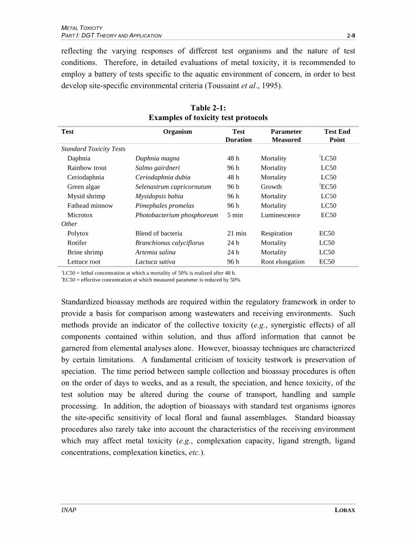
waters/effluents to aquatic biota (Table 2-1). In general, toxicity testwork is limited to a
few standard tests due to their recognition by regulatory agencies, and generally involves
determinations of mortality of standard test species (e.g., Daphnia magna and rainbow
trout). Such tests typically entail exposing test species to a solution at several dilutions,
and measuring organism mortality. Survivorship is then related to the concentration
gradient in order to determine the concentration at which 50% mortality occurs (e.g.,
LC50). The LC50 result is typically expressed as a "percent strength" of the original
effluent. Bacterial tests (e.g., Microtox
) have also been shown to afford reliable
measures of toxicity in a wide range of industrial wastewaters and impacted water courses
(Chang et al., 1981; Codina et al., 1993; Hao et al., 1996). A suite of less commonly
used tests also exist, including assessments of mortality to marine invertebrates (e.g.,
rotifers, Snell and Persoone, 1989) and lettuce root elongation (Miller et al., 1985) (Table
2-1). In general, the different tests exhibit varying sensitivities to metal toxicants,
METAL TOXICITY PART I: DGT THEORY AND APPLICATION 2-8
INAP LORAX
reflecting the varying responses of different test organisms and the nature of test
conditions. Therefore, in detailed evaluations of metal toxicity, it is recommended to
employ a battery of tests specific to the aquatic environment of concern, in order to best
develop site-specific environmental criteria (Toussaint et al., 1995).
Table 2-1: Examples of toxicity test protocols
Test Organism Test Duration
Parameter Measured
Test End Point
Standard Toxicity Tests
Daphnia Daphnia magna 48 h Mortality 1LC50
Rainbow trout Salmo gairdneri 96 h Mortality LC50
Ceriodaphnia Ceriodaphnia dubia 48 h Mortality LC50
Green algae Selenastrum capricornutum 96 h Growth 2EC50
Mysid shrimp Mysidopsis bahia 96 h Mortality LC50
Fathead minnow Pimephales promelas 96 h Mortality LC50
Microtox Photobacterium phosphoreum 5 min Luminescence EC50 Other
Polytox Blend of bacteria 21 min Respiration EC50
Rotifer Branchionus calyciflorus 24 h Mortality LC50
Brine shrimp Artemia salina 24 h Mortality LC50
Lettuce root Lactuca sativa 96 h Root elongation EC50 1LC50 = lethal concentration at which a mortality of 50% is realized after 48 h. 2EC50 = effective concentration at which measured parameter is reduced by 50%
Standardized bioassay methods are required within the regulatory framework in order to
provide a basis for comparison among wastewaters and receiving environments. Such
methods provide an indicator of the collective toxicity (e.g., synergistic effects) of all
components contained within solution, and thus afford information that cannot be
garnered from elemental analyses alone. However, bioassay techniques are characterized
by certain limitations. A fundamental criticism of toxicity testwork is preservation of
speciation. The time period between sample collection and bioassay procedures is often
on the order of days to weeks, and as a result, the speciation, and hence toxicity, of the
test solution may be altered during the course of transport, handling and sample
processing. In addition, the adoption of bioassays with standard test organisms ignores
the site-specific sensitivity of local floral and faunal assemblages. Standard bioassay
procedures also rarely take into account the characteristics of the receiving environment
which may affect metal toxicity (e.g., complexation capacity, ligand strength, ligand
concentrations, complexation kinetics, etc.).

International Network for Acid Preventi
3 Metal Speciation

3-1
3. Metal Speciation
Trace metals exist in a variety of inorganic and organic forms in aquatic systems, ranging
from simple hydrated molecules to large organic complexes. The biological availability,
and hence toxicity, of metals in aquatic systems is strongly dependent on the nature of the
metal species present. Accordingly, generating an understanding of the chemical form, or
"speciation", of metals in the environment is fundamental to predicting impacts to aquatic
biota. In the following chapter, the notion of metal speciation is introduced (Section 3.1).
A discussion of metal speciation in natural waters (Section 3.2) and mining-influenced
systems (Section 3.3) is then presented. The chapter concludes with a review of current
speciation techniques (Section 3.4) and a summary (Section 3.5).
3.1 Introduction
"Speciation" as defined by the International Union of Pure and Applied Chemistry
(IUPAC) refers to the atomic or molecular form of an analyte (Hill, 1997). Many
elements are commonly categorized according to their chemical forms, or species, in the
environment. The fundamental difference in chemical behaviour of various sulphur
species (SO4
2-, H2S, etc.) and nitrogen species (NH4
+, NO3
-, NO2
-, N2, etc.), for example, is
routinely acknowledged. Comparable classification of metal species in water is not
routinely carried out, however, largely due to a lack of user-friendly and cost-effective
techniques. The conventional practice of distinguishing “dissolved” (that which passes
through a 0.45 µm filter) and “total” metal concentrations (which include the particulate
phase) presents the only speciation method routinely conducted. Although such
dissolved/particulate separation can provide valuable information, it is widely recognized
that the speciation of metals exerts the fundamental control on biological uptake, and
hence toxicity. Increasing evidence suggests, for example, that the biological response of
aquatic organisms in the face of dissolved metal concentrations is proportional to the
activity of the free ions. Strongly complexed (thus, non-labile) and particulate metal
species are less available (Campbell, 1995). Thus, the determination of metal speciation
is as important as the determination of metal concentrations when assessing the impact of
trace metals to aquatic biota.
3.2 Speciation in Natural Waters
Metals exist in a wide variety of forms in natural waters. The nature of metal speciation
is a function of several variables, including the metal of consideration, pH, pE, salinity,
competing cations and the types and concentrations of metal complexing agents present.
In the following discussion, the speciation of metals in natural waters is reviewed with
METAL SPECIATION PART I: DGT THEORY AND APPLICATION 3-2
INAP LORAX
respect to dissolved metal species (Section 3.2.1). This is followed by an examination of
the influence of metal complexing agents (i.e., ligands) on metal speciation, as well as
examples of field and laboratory determinations. A brief examination of particulate metal
species is provided in Section 3.2.2.
3.2.1 “Dissolved” Metals
The simplest, most common categorization of metals in water is separation into
“dissolved” and “particulate” metal fractions by filtration. The fraction that passes
through a 0.45 µm filter is typically defined as “dissolved”, while the fraction collected by
the filter is termed “particulate”. "Dissolved" is operationally defined, and in a strict
sense is incorrect, as small particulates (i.e., <0.45 µm) will pass through the filter
membrane. Rather, the term "filterable" is a more correct term. In practice, the
“dissolved” component includes metal species that are truly dissolved, including
inorganic species (free metal ions and inorganic metal complexes) and organically
complexed metals, but also includes “colloidal” metal species. By definition, colloids are
particles which range in size from <0.01 to 10 µm, and are typically represented by clays,
Fe-oxyhydroxides, amorphous silica and calcium carbonate (Stumm and Morgan, 1981).
In the following sections, the "dissolved" component is analyzed in further detail with
respect to inorganic and organic speciation.
3.2.1.1 Inorganic Species
The concentration of metal on a cell surface that is available to an organism and that
influences its biological response has been shown to be proportional to the free metal-ion
activity in the bulk solution (Campbell, 1995). The free metal ion concentration itself,
however, often represents only a small portion of the total dissolved metal concentration.
Another fraction exists as complexes with assorted inorganic ligands. Important metal-
complexing inorganic ligands include CO3-, OH
-, Cl
- and SO4
2- ions. For example,
cadmium is known to form chloro complexes, whereas Co, Cu, Ni, Pb and Zn tend to
form complexes with carbonate ion (e.g., Tipping et al., 1998). These species are often
readily available to biota, because the complexes are typically weak and dissociate rapidly
to the free metal ion (see Chapter 2).
3.2.1.2 Organic Species
Until fairly recently, the speciation of dissolved metals was widely believed to be
dominated by inorganic metal species. In recent years, however, there has been an
increasing awareness that for many metals in natural waters, organic metal species
predominate with a wide variety of ligands involved (Bruland, 1989; Coale and Bruland,
1988; Kozelka and Bruland, 1998; Bruland, 1992; Nordstrom, 1996; Xue and Sigg,
1997). In most cases, complexation with organic ligands reduces metal bioavailability,
METAL SPECIATION PART I: DGT THEORY AND APPLICATION 3-3
INAP LORAX
because most organic-metal complexes are not readily transported across cell membranes.
Examples include complexes with fulvic and humic acids, which represent the byproducts
of polymerization and condensation reactions of natural organic matter. The latter form
complexes that are strong for some metals and fairly weak for others, but because they are
often abundant, their presence results in the dominance of organic complexes in many
natural waters.
A variety of particularly strong biologically produced organic ligands also exist in natural
waters. Examples include metallothioneins and phytochelatin. These compounds
represent low molecular weight, cysteine-rich metal-binding polypeptides that have been
identified to play detoxification roles in animals and plants, respectively (Roesijadi, 1992;
Lee et al., 1996). For example, at high inorganic cadmium concentrations, the marine
diatom Thalassiosira weissfloglii appears to export a cadmium-phytochelatin complex as
a detoxification mechanism (Lee et al., 1996). As additional examples, organic Cu-
complexing ligands have been observed to be released by many algae, including marine
diatoms (Zhou and Wangersky, 1989), marine microalgae (Emiliana huxleyi; Leal et al.,
1999) and cyanobacteria (Moffett and Brand, 1996). Recent evidence from freshwater
environments also suggests that strong metal-complexing ligands are produced by
phytoplankton (Xue and Sunda, 1997). Finally, anthropogenically produced ligands such
as EDTA are becoming increasingly common in aquatic environments. Because of its
strong affinity for many metals, EDTA-metal complexes can dominate metal speciation in
some settings (e.g., Sedlak et al., 1998).
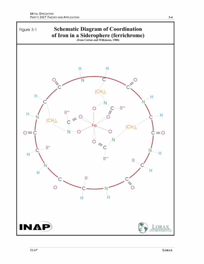
While in general organic ligands reduce metal bioavailability, there are some examples of
ligands which result in an increase in metal uptake by biota. Siderophores, for example,
are ligands with a high affinity for Fe that are released by organisms to facilitate the
transport of Fe into the cell. Siderophores (e.g., Figure 3-1) are diverse chemically, but
generally have in common chelating oxygen-donor-type functional groups (Cotton and
Wilkinson, 1980). Metals other than Fe may be passively transported into cells by such a
mechanism by substituting for iron, resulting in more rapid metal transport than would
otherwise be observed. However, this is predicted only to occur at low iron
concentrations, when organisms synthesize siderophores in order to meet their cellular
iron needs.
3.2.1.3 Effects of Ligand Concentration and Affinity on Speciation
Metal speciation is ultimately controlled by the combined influences of metal
concentration, ionic strength, pH, competing cations, ligand concentration and ligand
affinity. This can be readily demonstrated by the following calculations. The strengths
METAL SPECIATION PART I: DGT THEORY AND APPLICATION 3-4
INAP LORAX
METAL SPECIATION PART I: DGT THEORY AND APPLICATION 3-5
INAP LORAX
of metal complexing ligands can be expressed in terms of a stability constant, K, as
follows. For the reaction between a free metal divalent cation (M2+
) and a ligand (L),
M2+
+ L ↔ ML, the equilibrium constant can be described as:
K = ]][[
][2 LM
ML+ .
Since [ML] ≅ [Mdiss] – [M2+
], substituting and solving for ][
][2
dissM
M + yields:
][
][2
dissM
M + =
1][
1
+LK.
What becomes apparent from this relationship is that the proportion of free metal ion
depends on the product of the ligand concentration and the stability constant, K. Thus, a
low-concentration ligand that has an extremely high affinity for a metal can dominate the
metal speciation over a much more abundant, but weaker, metal ligand (provided both
ligands are present in excess of the metal).
3.2.1.4 Case Studies of Speciation in Natural Waters
Due to limitations in existing analytical techniques, the chemical structure of the vast
majority of organic ligands has not been determined. Nonetheless, electrochemical
techniques are capable of quantifying the concentration and strength of all existing
ligands, regardless of whether or not their precise chemical structure is known. As a
consequence, numerous studies have shown that metals are complexed in many
environments by organic complexes (Table 3-1). In seawater, for example, the dominant
species of Cd, Cu, Pb and Zn are dissolved organic complexes, (Bruland, 1989; Coale and
Bruland, 1988; Kozelka and Bruland, 1998; Wells et al., 1998). These metal-organic
complexes are extremely strong, being characterized by stability constants that range in
strength from ~109- ~10
12 (Kozelka and Bruland, 1998). Cu-complexing ligands of
varying strengths have also been identified. The strongest ligands are termed L1, the
second strongest L2 and the third-strongest L3 (Table 3-1). The dominance of a
particular ligand will depend on their relative concentrations.
The nature of metal speciation in freshwaters has not been characterized to the same
degree as in the marine environment. However, there is some information available on
organic complexation in freshwaters. For example, copper speciation in Lakes Greifen
and Lucerne (Switzerland) is dominated by complexation with strong ligands which are
present at much lower concentrations (~20-60 nM) than a considerably more abundant
class of weaker ligands (8 µM), presumably humic acids (Xue and Sunda, 1997). In a

METAL SPECIATION PART I: DGT THEORY AND APPLICATION 3-6
INAP LORAX
variety of European rivers, zinc has been observed to be ~70% complexed by organic
ligands with stability constants of ~107, resulting in a 30-50% reduction in zinc
bioavailability (Jansen et al., 1998). Organic species have also been shown to be
dominant for lead in anoxic freshwaters (Taillefert et al., 2000).
Table 3-1: Summary of representative metal and ligand concentrations,
the strength of metal-ligand complexes and the % contribution to metal speciation in a variety of freshwater and marine settings
Metal Location Metal Concentration
(nM)
Ligand Type Ligand Concentration
(nM)
Stability Constant (log K)
% Complexed
Cu Lakes Greifen
& Lucerne1
~10 L1 38±19E-9 15 >90
L2 1-3.5E-7 11-13
L3 8±2 E-6 8.6
Narragansett
Bay, RI2
13-28 L1 16-38 >12 >99
L2 15-40 8.8
L3 54-100 7.7
7-8
wastewater
treatment near SF
Bay3
20-200 L1 (synthetic chelates) ~1-10 11-14 5-80
L2 (humic substances) 340-490 ~7 5-50
San Francisco
Bay4
45 L1 13 >13.5 27
L2 20-30 9-9.6 52-65
Cd Narragansett
Bay, RI2
0.29-0.8 4 8.9 73-83
Zn Narragansett
Bay, RI2
16-72 11-48 9 51-97
European
Rivers5
90-4800 260-3300 6.4-7 55-88
Pb Narragansett
Bay, RI2
0.13-0.32 L1 0.8 10 67-94
L2 4-8 8.8
Ni wastewater
treatment near SF
Bay3,6
55-148 L1 (EDTA) 70 >12 30-100
L2 (humic substances) 430-740 6-7 1 Xue and Sunda, 1997.
2 Kozelka and Bruland, 1998.
3 Sedlak et al., 1997.
4 Donat et al., 1994
5 Jansen et al., 1998.
6 Bedsworth and Sedlak, 1999.
3.2.2 Particulate Metal Species
Metals may be hosted in particulate phases either as part of a mineral lattice, sorbed onto
particle surfaces, or as assimilated components in aquatic biota. In general, particulate

METAL SPECIATION PART I: DGT THEORY AND APPLICATION 3-7
INAP LORAX
metal phases tend to be less available, and hence less toxic, to organisms in comparison
to their dissolved counterparts. However, the ingestion of particles has been shown to be
an important mechanism of metal accumulation in filter feeding organisms (e.g., Roditi et
al., 2000).
Due the particle-reactive nature of many trace metals, particulate phases can play a
dominant role in metal speciation and behaviour. Many trace metals (e.g., Cu, Pb, Hg,
Cd, Zn, Ag) have been shown to be primarily associated with suspended and sedimentary
particulates in some freshwaters as opposed to dissolved phases (Davis and Leckie,
1978b; Nriagu et al., 1981; Laxen, 1985; Tessier et al., 1985). As a result, settling
particles are an important vector for the transfer of heavy metals to lake sediments,
thereby regulating the concentrations of dissolved species (Nriagu et al., 1981; Sigg,
1985; Jackson and Bistricki, 1995). Particulates in natural waters consist predominantly
of detrital particulate and colloidal organic matter, inorganic solids such as metal oxides
and hydroxides (e.g., SiO2, MnO2, FeOOH, Al2O3), algal skeletal remains, carbonates and
detrital aluminosilicates (e.g., clay minerals, feldspars) (Tessier et al., 1985). In general,
particulate organic matter often presents the major component of suspended material in
freshwaters, accounting for up to 70% of the total particulate fraction (Nriagu et al.,
1982). Colloidal metal species can be quantitatively significant in many environments
(e.g., Wells et al., 1998). In well-buffered mining- systems which receive inputs of acid
rock drainage, colloids often can host the bulk of the metal inventory. In such
environments, loadings of ARD can result in the precipitation of colloidal Fe-
oxyhydroxides which represent preferential sorption sites for many trace elements
(Jackson and Bistricki, 1995).
3.3 Metal Speciation in Mining-Impacted Systems
The metallurgical processing of base metal and gold ores involves the addition of various
reagents to enhance the recovery of desirable constituents. As a result, the chemical
composition of discharge waters can contrast greatly from waters in the receiving
environment. Such influences can potentially have a profound effect on metal speciation.
In the following section, the influence of these inputs on metal speciation is discussed.
Mining operations utilize a spectrum of chemical reagents in various stages of ore
treatment, mineral recovery and effluent treatment (Table 3-2). During milling
operations, for example, various inorganic (e.g., activators) and organic reagents (e.g.,
frothers and collectors) may be added to the process stream. Accordingly, variable
quantities of such components inevitably report to tailings impoundments. For many
operations, water balance considerations require the discharge of tailings pond overflow
to receiving waters, and as a result, various metallurgical and/or treatment products are

METAL SPECIATION PART I: DGT THEORY AND APPLICATION 3-8
INAP LORAX
discharged to the environment. The effect of process reagents on metal bioavailability in
natural systems is poorly constrained. However, given the nature of functional groups
characteristic to the suite of organic reagents utilized (e.g., dithiocarbonates, carboxylic
acids, esters, organo-phosphates, etc.) it is likely that metal speciation is strongly
influenced in certain environments. In addition, the presence of high-affinity inorganic
products such as cyanide compounds, chloride, and sometimes sulphate will undoubtedly
have an effect on metal speciation. In particular, metal-CN complexes may have
considerable importance in systems that receive loadings from gold-mining operations.
The influence of such chemicals on metal speciation, bioavailability and toxicity requires
further research (see Chapter 4).
Table 3-2: Possible mining-related waste products resulting from ore processing, waste treatment and mine-site run-off
Process Possible Waste Products
Flotation Alkaline waste stream
Sulphate Metal hydroxides
Frothers (organic reagents, e.g., C6-C9 alcohols, pine oil, cresol) Activators (e.g., CuSO4, Na2S) Depressants (e.g., lime, NaCN, ZnSO4) Collectors (e.g.¸ Xanthates)
Pressure Oxidation
Ferric sulphates, arsenates , jarosites
Metal hydroxides
Cyanide Destruction/Recovery
Cyanide, Cyanate, thiocyanate
Ammonia Hydroxide sludges Cyanide salts Chlorine
ARD Treatment
Neutralization/Precipitation: Alkaline waste stream Hydroxide sludges Sulphates Sludge flocculaters (e.g., acrylamide)
Solvent Extraction: Carboxylic acids Sulphonic acids Alcohols Amines
Activated Carbon: Organics
Effluent treatment before discharge EDTA
Mine Site Run-off ARD
Petro-chemicals Blasting reagents (ammonia, nitrate) Road salt

METAL SPECIATION PART I: DGT THEORY AND APPLICATION 3-9
INAP LORAX
A wide range of synthetic additives may also influence metal speciation and
bioavailability in receiving waters. EDTA, for example, may be added to waste streams
prior to discharge in order to minimize toxicity to biota in downstream environments.
EDTA is a very strong ligand which favours complexation with many trace metals (e.g.,
Cu, Zn, Cd, Pb, Hg). Synthetic frothing agents, representing mainly high molecular-
weight alcohols (e.g., methyl isobutyl carbinol), may also influence the bioavailability of
metals in receiving waters.
The dynamics of mixing between effluent and the receiving waters can also affect metal
speciation. As outlined above, the flocculation of ARD inputs upon contact with pH-
neutral watercourses can result in the formation of colloidal Fe-oxyhydroxides. This
process can result in the co-precipitation and scavenging of metals from solution. In
addition, metal speciation and bioavailability can be significantly affected in systems
where effluents are discharged into waters with significant quantities of metal-
complexing ligands. There are two common scenarios where this can occur: 1) the
discharge of mining effluent into DOC-rich waters; and 2) the discharge of mining
effluent into seawater. The addition of metal-bearing effluents to DOC-rich freshwaters
will result in the complexation of a certain fraction of the metal inventory, thereby
potentially decreasing metal bioavailability. In this situation, the mixing dynamics
becomes important in influencing the rate at which the metal comes in contact with the
complexing ligands. Similarly, where relatively-fresh effluent is discharged into higher
ionic strength waters (such as seawater), significant flocculation of metal-bearing colloids
can occur, resulting in significantly lower concentrations of dissolved metals over short
distances and time intervals (e.g., Boyle et al., 1976; Sholkovitz et al., 1976; Karbassi and
Nadjafpour, 1996).
3.4 Speciation Techniques
A number of techniques currently exist for quantifying aqueous metal speciation. Among
these, three approaches have great potential as speciation tools. These include: 1)
diffusive gradients in thin films (DGT); 2) voltammetry; and 3) supported liquid
membrane techniques (SLM). These three approaches are described in turn below.
3.4.1 DGT
Diffusive Gradients in Thin Films (DGT) represents one of the most promising
techniques for determining the concentration of labile metal species in aquatic systems
(Zhang and Davison, 1995). This method is discussed in detail in Chapter 4, and
therefore only a brief description is presented here. The DGT device consists of a ~4 cm-
diameter disk, comprising a filter membrane underlain by a polyacrylamide gel layer,
METAL SPECIATION PART I: DGT THEORY AND APPLICATION 3-10
INAP LORAX
which is in turn underlain by a trace-metal-adsorbing gel-embedded resin. Metals diffuse
from solution across the filter and gel layers to the underlying resin, where metal sorption
takes place. The resin only adsorbs free and kinetically-labile metal ions. This approach
therefore provides a better measure of biologically-available metals than do dissolved or
total metal concentrations. The principal advantages of the DGT device include the
possibility of in situ deployment, low risk of sample contamination, sample pre-
concentration and relative ease of use.
3.4.2 Voltammetry (ASV and AdCSV)
Voltammetry is a technique in which the concentrations of labile metal species are
determined from a current measured in solution as a metal is taken up into, or released
from, a mercury-containing electrode (Sawamoto, 1999). The instrumentation consists of
a voltammetric analyzer, a three-electrode cell (working electrode, reference electrode
and counter electrode) and a computer for automated measurements and data acquisition.
The most commonly used working electrodes are hanging drop mercury electrodes
(HDME) and rotating mercury-film electrodes (MFE) (Achterberg and Braungardt, 1999).
The advantage of HDME is its reliability, while MFE offers increased sensitivity due to
the concentration of metals into a smaller volume of mercury film. MFE, however, is
subject to interferences as surfactants collect on the electrode surface, while HDME is not
because a new mercury drop is used for each assay. One recent means of overcoming this
limitation for MFE is to cover the electrode surface with a semi-permeable membrane
that permits transport of ions but excludes the potential interferences (Tercier et al.,
1998a, 1998b). Strengths of voltammetric approaches include low detection limits (10-10
-
10-12
M), multi-element capability and suitability for ship-board determinations
(Achterberg and Braungardt, 1999). There are two commonly used variants of
voltammetry, including anodic stripping voltammetry (ASV) and adsorptive cathodic
stripping voltammetry (AdCSV).
In ASV, the metal ion of interest is deposited on the mercury electrode via the reduction
of the metal to a metallic state and subsequent amalgamation with the mercury. This is
followed by a voltammetric scan towards more positive potentials, during which the
mercury-bound metal is oxidized and the current produced is determined. The identity of
the metal is dictated by the potential of the peak, while the concentration is proportional
to the height of the peak. Absolute concentrations are inferred by the standard additions
method, because the sensitivity may vary between samples of different ionic strength and
different concentrations of surfactants and natural organic compounds. Thus, the species
measured are operationally defined to include free metal ions and species that can
dissociate to free metal ions within time scales of ~10-3
s. ASV has been widely used,
particularly in metal speciation studies in the marine environment (Bruland, 1989; Coale
METAL SPECIATION PART I: DGT THEORY AND APPLICATION 3-11
INAP LORAX
and Bruland, 1988; Achterberg, et al., 1994; dosSantos, et al., 1996; Kozelka and
Bruland, 1998; Wells et al., 1998).
In AdCSV, a specific ligand which is added to the sample forms a complex with the metal
of interest and adsorbs onto the surface of the electrode. A voltammetric scan towards
more negative potentials follows and the resulting current is measured. The current
produced results from the reduction of a reducible group on the ligand or of the metal
itself in the adsorbed complex. As in ASV, the identity of the metal is determined by the
potential, while the concentration is determined from the size of the peak. The AdCSV
approach has been widely used for metal determinations in seawater (Donat et al., 1994)
as well as in freshwater (Xue and Sunda, 1997).
ASV and AdCSV methods are characterized by certain disadvantages. First, both
techniques are typically conducted in the laboratory, often many hours or days after
sample collection. Given that changes in metal speciation can occur over these time
scales, the representativeness of such data are questionable. This shortcoming, however,
has recently been overcome with the development of a voltammetric in situ profiling
(VIP) probe which allows in situ measurements to depths of 500 m (Tercier-Waeber et
al., 1999). Another significant limitation of voltammetric approaches is that the test
medium requires the presence of small amounts of electrolytes in solution. Therefore,
applications to low-ionic strength solutions (e.g., freshwaters) are limited. Furthermore,
it is difficult to carry out voltammetric determinations in solutions of poorly characterized
salinity because the signal is dependent on the ionic strength. Voltammetric techniques,
therefore, have most frequently been used in seawater, where the ionic strength is well
characterized and essentially constant. Nevertheless, there are successful examples of
voltammetric studies in freshwaters (Cheng et al., 1994; Jansen et al., 1998; Xue and
Sunda, 1997; Vega et al., 1995).
3.4.3 Supported Liquid Membrane
The supported liquid membrane (SLM) technique closely mimics the mechanism of metal
uptake by biota. In this approach, labile metal species are transported across a membrane
and are pre-concentrated into a solution on the opposite side of the membrane (Tercier-
Waeber et al., 2000; Keller et al., 1994; Parthasarathy and Buffle, 1994; Keller and
Buffle, 2000). In detail, the aqueous sample is pumped past a porous membrane
embedded with a non-water-miscible solvent in which is dissolved a hydrophobic ligand
(Figure 3-2). Labile metal species are complexed by the ligand, transported across the
membrane by diffusion and accumulated in a second solution on the other side that
contains a ligand of greater strength than the hydrophobic ligand-transporter (Figure 3-2).
By carefully controlling the ligand strengths, flow rates and solution volumes, only the

METAL SPECIATION PART I: DGT THEORY AND APPLICATION 3-12
INAP LORAX
labile metal species can be transported, and pre-concentration can occur, permitting
quantification of “labile” species at the low levels found in many natural waters. The
strengths of SLM include:
1) the technique mimics transport across biological membranes (see Chapter 2);
2) pre-concentration permits use of the technique at very low metal concentrations;
and
3) the technique can be tailored to mimic biological uptake of different metals via
adjustment of the ligands used.
Disadvantages include the degree to which the approach must be optimized for each
metal and the sophistication of the equipment, as well as limited prospects for in situ
deployment in the field.
3.4.4 Other
The speciation techniques described above represent the most promising techniques at the
current time for low-level determinations of free-metal concentrations in natural waters.
Another technique involves the use of Ion-Specific Electrode (ISE). ISE techniques,
which have been developed for Cu and Cd, are currently limited in their application due
to poor detection limits. Additional techniques being utilized include batch treatment of
water samples with ion exchange resins (Muller and Kester, 1991), liquid
chromatography-inductively coupled plasma mass spectrometry (Vela and Caruso, 1993),
the Wageningen Donnan Membrane technique (Temminghoff et al., 2000) and
electrospray ionization mass spectrometry (Schramel et al., 1998; Ross et al., 2000).
These other approaches do not have the broad applicability of the above-mentioned
techniques, however, and are thus not discussed in detail.
3.5 Summary
The relative proportions of the various metal species in natural waters depend on the
concentrations of the metals and the concentrations and strengths of the various ligands
present. A variety of analytical techniques has been used to quantify metal speciation in
natural waters. Virtually all of the techniques suffer inadequacies that limit their general
use. For example, most existing techniques must be carried out in a laboratory rather than
in situ. Furthermore, most require expensive instrumentation that must be used by a
highly trained operator. The DGT method, however, can be carried out in situ at modest
cost by relatively untrained personnel. Thus, the DGT approach has tremendous potential
for use as a routine water-quality monitoring tool.
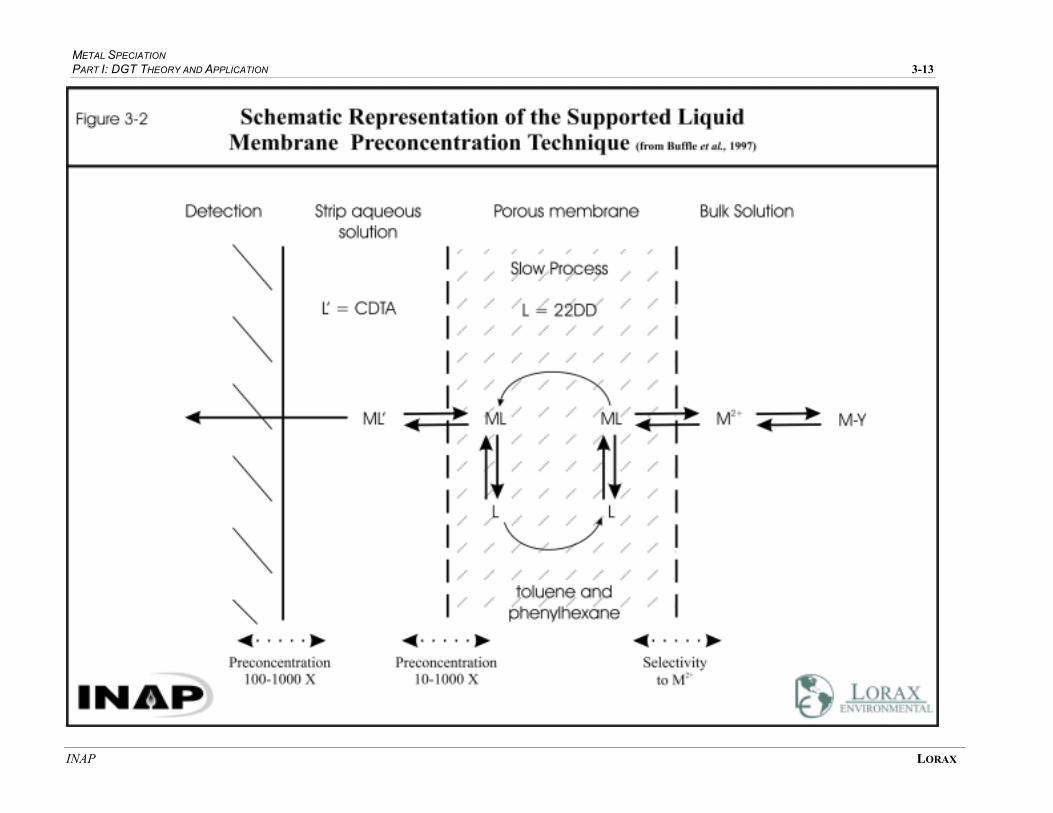
METAL SPECIATION PART I: DGT THEORY AND APPLICATION 3-13
INAP LORAX

International Network for Acid Preventi
4 DGT
4-1
4. DGT
4.1 Introduction
The collective understanding of trace metal cycling in the environment has been advanced
significantly since the early 1980’s with the advent of “ultra-clean” trace metal protocols
for sample collection, handling and analysis (Bruland, 1979; Nriagu et al., 1993). Prior to
this time, attempts to study the behaviour of trace metals in aquatic systems were
hindered by problems of contamination, and as result, the data generated were often not
representative. Despite improved sampling techniques and insight into trace metal
behaviour and toxicity, the regulatory framework for the environmental assessment of
water quality (i.e., the reliance on total metal concentrations) has remained virtually
unchanged. For example, it is acknowledged that total metal concentrations are a poor
proxy for metal bioavailability, particularly where high suspended sediment loads exist.
Although it is recognized that measurements of total metals yield limited site-specific
information with respect to bioavailability and toxicity, there is currently a dearth of
economic and user-friendly tools for routine determinations of metal speciation. Efforts
to ascertain metal toxicity typically utilize standard bioassay protocols. The use of
polarographic techniques to assess metal speciation, effluent toxicity and complexation
capacity have been used less frequently. The primary limitation with these latter
approaches, however, relates to the potential for alterations to metal speciation between
sample collection in the field and analysis in the laboratory. Sample turn-around, for
example, is often on the order of days for both bioassays and speciation analyses. In situ
bioassays and/or autonomous in situ samplers have been used on occasion, but these
approaches are often prohibitively expensive, difficult to use routinely, and usually
require operation by highly-trained personnel.
DGT (diffusive gradients in thin-film) represents a relatively new approach to water
sampling which essentially obviates many of the limitations outlined above (Zhang and
Davison, 1995). In general, DGT affords in situ determinations of metal speciation in
aquatic systems by selectively accumulating labile metals. Accordingly, the technique
allows inferences to bioavailability and toxicity. Furthermore, since DGT passively
accumulates labile metals from solution while deployed in situ, contamination problems
associated with water collection and filtration are eliminated. Given the speciation
capabilities of DGT, in conjunction with its affordability and ease of use, DGT has
considerable potential as a routine monitoring tool in mining-related environmental
studies (McNee and Robertson, 1998).
DGT PART I: DGT THEORY AND APPLICATION 4-2
INAP LORAX
The following Chapter 5 details the theory and application of DGT technology.
Subsequent to a discussion of the theoretical considerations (Section 4.2), applications of
the approach to assessments of speciation, toxicity, complexation kinetics and
complexation capacity are discussed (Section 4.3). The section concludes with an overall
assessment of the considerations for DGT application and associated technique
limitations (Section 4.4), as well as identifying data gaps and areas for future research
(Section 4.5).
4.2 DGT Theory and Design
The following section presents the theory and design of DGT. Following a detailed
discussion of DGT theory, the calculations used to generated DGT values are described.
The section concludes with a description of the DGT sampler with respect to
configuration, deployment and analysis.
4.2.1 DGT Theory
The theory behind DGT is based on the diffusional characteristics of metals in a hydrogel
and on the sorption properties of a metal-binding resin (Zhang and Davison, 1995; Davison et al., 2000). Specifically, the technique utilizes a hydrogel layer to control the
diffusive transport of metals in solution to a cation-exchange resin. The laws of diffusion
are well known, while the characteristics of the diffusive path afforded by the DGT
sampler are reasonably well defined. In addition, since the cation exchange resin in DGT
(Chelex) is selective for free and/or weakly complexed species, it affords a proxy for the
labile fraction of metals in solution which is believed to approximate the bioavailable
fraction. . Other methodologies have implicitly acknowledged the value of using resins
such as Chelex (Paulson, 1986; Pai et al., 1990; Chakrabarti, et al. 1994) or 8-
hyroxyquinoline (Beauchemin et al., 1987; Sturgeon et al., 1982) to extract metals in situ,
but most approaches typically involve the use of pumps or autonomous samplers. DGT
differs from other resin techniques in that it uses the laws of diffusion to control the flux
of metals to the resin layer. In this manner, the concentration of labile metal species in
solution can be reasonably quantified (Zhang and Davison, 1995; Denny et al., 1999;
Davison et al., 2000).
DGT utilizes a three layer system: 1) a resin-impregnated hydrogel layer; 2) a hydrogel
diffusion-layer; and 3) and a filter membrane (Figure 4-1). The innermost two gel layers
are fabricated from a polyacrylamide hydrogel. Polyacrylamide is a hydrous polymer
consisting of acrylamide-polymer chains, typically linked with bis or agarose cross-
linkers (Chramback, 1985). Chelex resin is a strong metal complexing agent and rapidly
binds free and/or kinetically-labile metal species (Paulson, 1986; Pai et al., 1990).

DGT PART I: DGT THEORY AND APPLICATION 4-3
INAP LORAX
Therefore, the resin layer serves as a sink for labile metal species which diffuse through
the polyacrylamide diffusion-layer (Figure 4-1). The filter membrane
(pore size = 0.45 µm) protects the fragile polyacrylamide surface and isolates it from
particles.
During deployment of the DGT sampler, dissolved metal species in solution freely diffuse
through the diffusive boundary layer (DBL), the filter membrane and the polyacrylamide
gel-layer (Figure 4-1). The DBL is the layer of water adjacent to all solid surfaces where
flow velocity is zero; its thickness varies inversely with flow but typically ranges from a
single molecule to millimetre-order distances (Santschi et al., 1983). Thus, there is a
continuum of flow velocities adjacent to the solid surface ranging from a zero velocity
very near the surface to a maximum velocity at some finite distance. Within the DBL
zone adjacent to the DGT surface, mass transport occurs by molecular diffusion.
Similarly, since approximately 90% of the polyacrylamide gel is water, and because the
nature of the polymer matrix is open to movement at the molecular scale, transport of
metals through the gel also occurs by molecular diffusion (Davison and Zhang, 1994;
Krom et al., 1994; Zhang and Davison, 1999). Most hydrated cations fall within the
range of 0.2 to 0.3 nm diameter and thus diffuse through the DGT hydrogel, which hosts a
functional pore size greater than 2 to 5 nm.
Although diffusion through the hydrogels can be relatively unconstrained, the gels used in
DGT consist of ~10 % cross-linked polymer. This constrains the permeability of the gel
and requires that neutral and charged diffusing ions follow a tortuous path, which lowers
their effective diffusion coefficients. Such effects become more pronounced as the gel
becomes tighter. Furthermore, ionic strength, pH, and solution composition can influence
the rate of diffusion by affecting the behaviour of functional groups on the
polyacrylamide, which may become ionized and interact specifically with diffusing
charged species. Collectively, these features should reduce slightly the diffusion
coefficients of ions relative to those in water. Waters with very low cation concentrations
(<2 x 10⁻⁴
M) also pose a challenge. In such settings, the sodium form of polyacrylamide
used in the gel samplers can establish steep negative concentration gradients of Na+ from
the gel to the sample water (Alfaro-De la Torre et al., 2000). To preserve
electroneutrality, these are compensated by steepened concentration gradients of cations
in the opposite direction. These enhance the flux of cations to the gel, causing their
"labile" concentrations to be overestimated. In most mining-impacted regions, this is not
of importance because surface waters typically have higher ionic strengths. But in pristine
natural waters on the Canadian Shield, for example, this co-diffusion effect may be
important. Such constraints need to be kept in mind in DGT field applications.

DGT PART I: DGT THEORY AND APPLICATION 4-4
INAP LORAX
DGT PART I: DGT THEORY AND APPLICATION 4-5
INAP LORAX
Within the Chelex gel-layer, labile metal species are rapidly removed from solution to
metal-binding sites on the resin. Metal consumption within the resin layer results in an
effective "zero" concentration of labile metal species adjacent to the resin surface (Figure
4-1). Due to the presence of this "metal sink", concentration gradients are established
within the DGT unit, and extend into solution through the DBL (Figure 4-1). If
differences between the diffusion coefficients in the DBL, the protective filter membrane,
and the hydrogel are present, contrasting concentration gradients will be established, as
shown in Fig. 4-1. The different gradients reflect the fact that at steady-state, the flux
through each layer must be identical.
Metal ions accumulate in the Chelex layer by diffusing along the concentration gradients
from solution to resin in accordance with Fick’s laws of diffusion and the well-defined
configuration of the DGT sampler (Figure 4-1). Diffusion of most ionic and molecular
species over these distances (i.e., < 1 mm) occurs on the order of seconds to minutes (Li
and Gregory, 1974; Manheim, 1970). Thus, both steady-state and stable concentration
gradients are established rapidly (i.e., < 5 minutes) within the DGT sampler upon
deployment in the sample medium. Therefore, while the DGT unit is deployed, labile
metal species accumulate at a constant rate in a predictable and reproducible fashion. The
concentration of labile metal species can then be calculated knowing the mass of metal
accumulated on the resin, the diffusion coefficient for the metal, and the deployment time.
A limit on the accuracy of the assayed concentration is imposed by uncertainty in the
diffusion coefficient used in the calculation. For example, Alfaro-De la Torre et al. (2000)
determined that the tracer diffusion coefficient of Cd in gel (DCd) was 0.9 that of water,
while Zhang (cited in Alfaro-De la Torre et al (2000)) more recently derived a DCd of 0.8.
The difference was ascribed to batch-to-batch variations in the agarose-derivative cross-
linker. Thus, although estimated gel diffusion-coefficients are available for most
environmentally-significant trace metals (Zhang and Davison, 1995), they are likely to be
adjusted as research on the DGT technique continues.
The influence of the DBL is related to the flow conditions adjacent to the sampler surface.
Specifically, the impact of the DBL is most pronounced in stagnant fluids because the
thickness of the DBL is greatest when the interfacial velocity (flow) at the gel surface is
lowest (Gundersen and Jorgensen, 1990). In low-current fluids, such as the deep waters
of a lake or ocean, the DBL is often in the range of 0.5 to 1 mm thick (Santschi et al.,
1983). This thickness is comparable to that of the polyacrylamide layer within the DGT
unit (typically 0.4 to 0.8 mm); in such cases, the DBL exerts a significant influence on the
flux of metal to the resin layer. By contrast, in high-velocity fluids such as flowing
streams, the DBL thickness can be negligible relative to the gel sampler thickness. Under
such conditions (i.e., cm/s order flow rates), the diffusive path length from solution to
resin layer is negligibly influenced.

DGT PART I: DGT THEORY AND APPLICATION 4-6
INAP LORAX
Direct measurements of the thickness of the DBL are difficult and impractical. Given
that the thickness of the DBL varies inversely with flow, and since flow is variable in
time and space, a single direct measurement of DBL thickness is not representative.
Rather, where DBL thickness is deemed to be an issue (i.e., in quiescent waters), it is
more effective to measure it indirectly by using multiple DGT units with varying
diffusive-gel thicknesses. Since the DBL thickness and the free metal concentration in
solution are identical for DGTs with varying gel thicknesses, the DBL thickness can be
determined mathematically. The calculation of the DBL correction factor is outlined in
detail in Section 4.2.2. This calculation assumes that the diffusion coefficients adopted
for the ions of interest are the same for all samplers irrespective of gel thickness. This
assumption has not yet been rigourously tested. Further, changing the thickness of the gel
layer will change the size of the pool of labile metal that can dissociate within the sampler
and react with the Chelex; this could have an impact on the calculated labile metal
concentration (Zhang and Davison, 1995), although in most cases, this should be very
minor.
The manner in which DGT sequesters metals from solution serves to pre-concentrate
metals. Specifically, the DGT sampler continually accumulates metals during the
deployment period, such that the final mass of metal on the resin may be equivalent to
that present in many millilitres or litres of water. Upon processing of the DGT for
analysis, the total mass of metal on the resin is extracted into ~1 mL of acid. This pre-
concentration process has two principal advantages. First, the method affords very low
detection limits, with the effective sensitivity increasing with deployment time. Second,
because DGT metals are extracted into a medium (usually nitric acid) which is desirable
for direct injection into most analytical instruments (e.g., ICP-MS and GFAAS),
problems associated with matrix effects are obviated. Conventional analyses of high
ionic-strength solutions, for example, generally involve labour-intensive extraction
procedures which increase the chances for contamination. In addition, since Chelex does
not preferentially adsorb the anions common to salt waters (e.g., Cl-, SO4
2-, etc.), such
constituents are effectively eliminated from the sample matrix.
4.2.2 Calculation of Concentration
The use of DGT for trace metal determinations is in many respects simpler than
conventional water sampling methods. However, the calculation of actual DGT-metal
concentrations is more involved. The concentration of labile metals in solution is
calculated using the measured metal ion inventory on the resin, the sampler exposure
time, and the temperature-corrected molecular diffusion coefficient for the metal of
interest. This section explains how the “free” or “bioavailable” metal concentrations are
determined using DGT.

DGT PART I: DGT THEORY AND APPLICATION 4-7
INAP LORAX
Calculation of the free metal ion concentration is based on measurement of a metal flux
(e.g., g cm-2 s-1) through the gel and involves the following steps. The flux of trace metals
may be quantified by applying Fick’s first law of diffusion as expressed by the following
equation:
F = DCb
∆g (1)
where F is the flux of trace metal ions diffusing from the bulk solution to the resin layer,
Cb is the concentration of the labile metal in bulk solution, ∆g is the thickness of the
diffusion layer (i.e., gel + filter) and D is the temperature-corrected diffusion coefficient
for the free hydrated metal ion in the gel (Zhang and Davison, 1995; Krom et al., 1994).
The equations below effectively assume a single average D for all three layers (the DBL,
the filter, and the gel) and thus represent the simplest approach to the determination of Cb.
Where D in the gel is close to that of water, this approach will introduce little inaccuracy.
As Dgel diverges from that in water, however, some inaccuracy will be incorporated,
particularly where the DBL is thick, as in stagnant waters; this can be minimized by
adopting the more rigourous approach of Alfaro-De la Torre et al. (2000), in which
different diffusion coefficients are assigned to the gel layer and the combined filter/DBL
layer pair. Because the difference between the two approaches will be very small in terms
of the Cb that each determines, we describe only the simpler calculation here.
Since flux is equal to mass (M) per unit area (A) per unit time (t), equation (1) can be
rewritten as:
g
tADCM b
∆= (2)
Thus, the concentration of free metal ion in the solution (Cb) to be expressed as:
DtA
gMCb
∆= (3)
where M is the mass of metal accumulated on the resin, t is the deployment time, and A is
the surface area of the gel layer. The value of M is determined analytically, typically by
Inductively Coupled Plasma Mass Spectrometry (ICP-MS). The thickness of the gel
layer (∆g) is formed to precise specifications during the manufacturing process, but for
accurate assays it should be measured prior to deployment because there can be slight
batch-to-batch differences in thickness. The diffusion coefficients of metals in
polyacrylamide gel have been measured (Davison and Zhang, 1995) and are typically
less than those observed in water, reported by Li and Gregory (1974). As noted above,
there can also be differences in diffusion coefficients from one batch of gel to the next.
This imposes a constraint on accuracy that can probably be on the order of +10 %.
Because diffusion coefficients are temperature dependent, it is essential to measure the

DGT PART I: DGT THEORY AND APPLICATION 4-8
INAP LORAX
temperature of the water in which the gel sampler is deployed. The only remaining
variable is deployment time, which must be accurately recorded for a reliable
measurement. Thus, based on the amount of metal measured on the resin and some
simple calculations, the concentrations of labile metal in solution can be estimated.
In cases where the DBL thickness (x) is consequential, equation (3) becomes:
DtA
xgMCb
)( +∆= (4)
Equation (4) has two unknowns (Cb and x); thus, in order to solve for both variables, a
second equation is developed through deployment of an additional DGT unit having a
different value for ∆g (Figure 4-2). For example, if two samplers are deployed having gel
layer thicknesses (∆g) of 0.4 and 0.8 mm, respectively, then:
DtA
xM
DtA
xM
DtA
xgMCb
)8.0)(()4.0)(()( 8.04.0 +=
+=
+∆= (5)
Cb, D, t and A are constants and M0.4 and M0.8 are measured, simplifying the equation to:
)(
)8.0)(()4.0)((
4.08.0
8.04.0
MM
MMx
−−
= (6)
The DBL thickness (x) can now be solved as can the labile metal concentration in
solution (Figure 4-2). Note that this calculation ignores the possible effect introduced by
increasing the size of the labile metal pool in the thicker gel layer. If significant
concentrations of metal complexes in that pool dissociate within the gel and add to the
Chelex-bound metal concentration, then Cb can be overestimated. Under these
circumstances, Equation 5 would be difficult to solve accurately. Further work is
required to determine the importance of this effect in Cb estimates. It should be of most
significance where dissolved metal concentrations are low and thus should not be of
concern in impacted mine-site regions.
In summary, determining free metal-ion concentrations using DGT requires
measurements of: 1) the mass of metal accumulated on the resin; 2) the water
temperature; and 3) the deployment time, followed by a series of flux calculations. In
stagnant or slow-flowing waters it is necessary to deploy gel samplers of two different
thicknesses to reduce uncertainties caused by the diffusive boundary layer. In some cases
however, especially where ambient dissolved metals concentrations are low, other
uncertainties will be introduced by the dual-thicknesses approach.
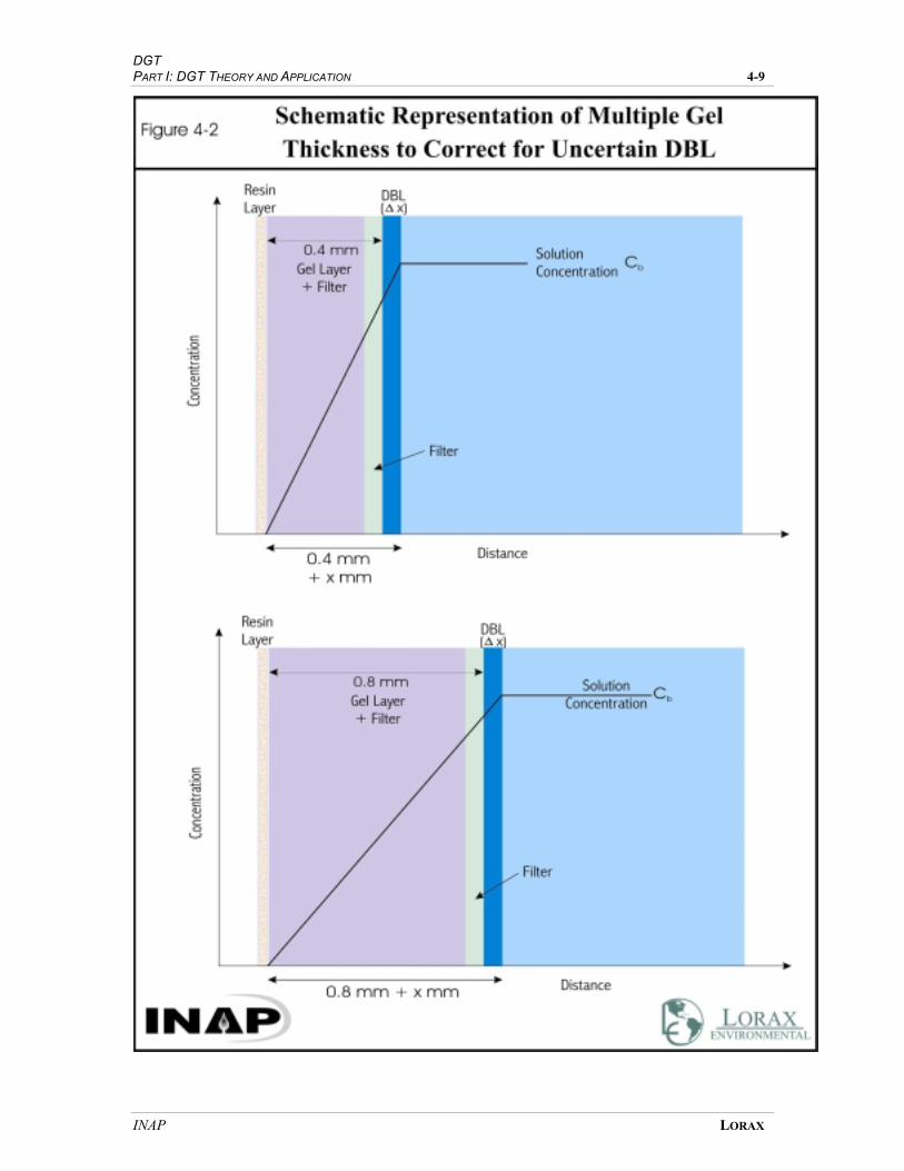
DGT PART I: DGT THEORY AND APPLICATION 4-9
INAP LORAX
DGT PART I: DGT THEORY AND APPLICATION 4-10
INAP LORAX
4.2.3 The DGT Sampler
As outlined above, the DGT sampler utilizes a three-layer system, consisting of a resin-
impregnated gel layer (metal-binding layer), an outer gel layer (diffusion layer) and a
filter membrane. Each layer is cut to specifications and placed in sequence on a plastic
base (Figure 4-3). A plastic outer-sleeve is placed over the base in order to secure the
layers, to maintain an even surface, and to inhibit water ingress into the resin-gel.
Hydrated DGT samplers are stored refrigerated in sealed plastic bags until immediately
before deployment. Deployment typically involves suspension of the unit in situ or in a
stirred solution in the laboratory (or in the field) for a fixed period of time. During the
deployment interval, time and temperature are recorded. Upon retrieval, the DGT units
are rinsed with distilled deionized water and stored refrigerated in sealed plastic bags to
avoid dehydration and potential contamination.
Processing of DGT samplers is performed under class 100 clean-room conditions. The
samplers are disassembled and the resin layer analyzed for metal content. Analysis can
occur via: 1) acid-extraction of the resin layer followed by metal analysis of the extract
(e.g., via ICP-MS); or 2) through direct analysis of the resin beads themselves by
techniques such as proton induced x-ray emission (PIXE; Davison et al., 1997a) or laser
ablation (Davison et al., 2000). Metal determinations involving direct analysis of the
Chelex beads by PIXE or laser ablation are comparatively non-destructive and afford the
opportunity to observe spatial distributions of metals. This ability does not offer
advantages for water column applications, but does provide the opportunity to study ultra-
fine scale structure in certain environments such as microbial mats (Davison et al., 1997a)
or sediment pore waters (Harper et al., 1999a) (see Chapter 5).
4.3 DGT Applications
DGT techniques afford wide-ranging applications in various fields of environmental
chemistry which utilize measurements of free or labile metal species. The following
sections describe the use of DGT as it applies to measurements of speciation (Section
2.3.1), toxicity (Section 4.3.2), complexation kinetics (Section 4.3.3) and complexation
capacity (4.3.4). Examples of field and laboratory data are also presented.
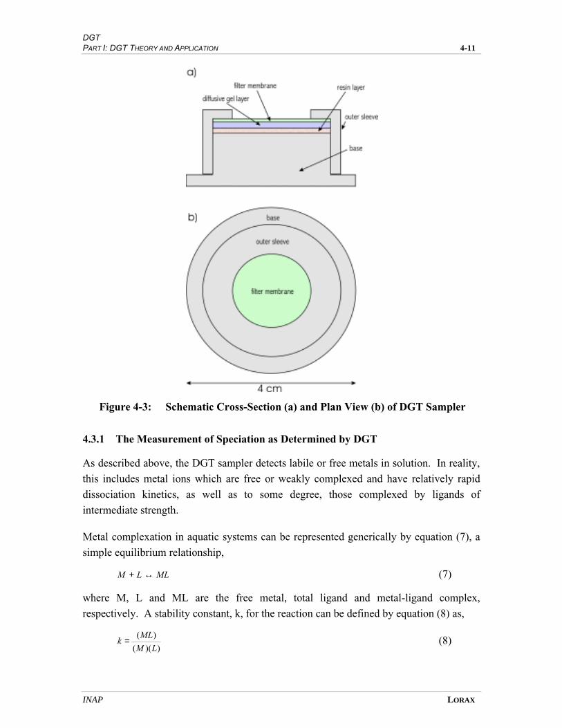
DGT PART I: DGT THEORY AND APPLICATION 4-11
INAP LORAX
Figure 4-3: Schematic Cross-Section (a) and Plan View (b) of DGT Sampler
4.3.1 The Measurement of Speciation as Determined by DGT
As described above, the DGT sampler detects labile or free metals in solution. In reality,
this includes metal ions which are free or weakly complexed and have relatively rapid
dissociation kinetics, as well as to some degree, those complexed by ligands of
intermediate strength.
Metal complexation in aquatic systems can be represented generically by equation (7), a
simple equilibrium relationship,
MLLM ↔+ (7)
where M, L and ML are the free metal, total ligand and metal-ligand complex,
respectively. A stability constant, k, for the reaction can be defined by equation (8) as,
))((
)(
LM
MLk = (8)
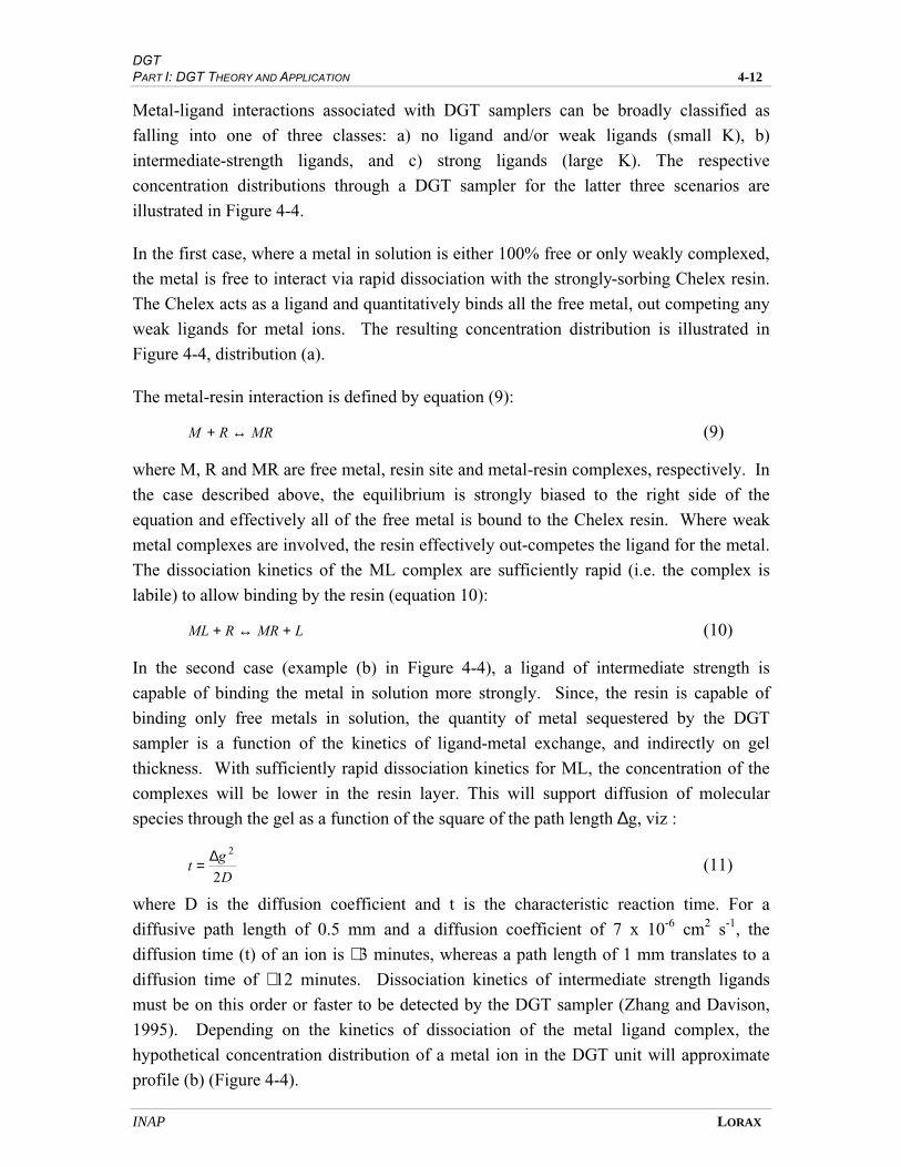
DGT PART I: DGT THEORY AND APPLICATION 4-12
INAP LORAX
Metal-ligand interactions associated with DGT samplers can be broadly classified as
falling into one of three classes: a) no ligand and/or weak ligands (small K), b)
intermediate-strength ligands, and c) strong ligands (large K). The respective
concentration distributions through a DGT sampler for the latter three scenarios are
illustrated in Figure 4-4.
In the first case, where a metal in solution is either 100% free or only weakly complexed,
the metal is free to interact via rapid dissociation with the strongly-sorbing Chelex resin.
The Chelex acts as a ligand and quantitatively binds all the free metal, out competing any
weak ligands for metal ions. The resulting concentration distribution is illustrated in
Figure 4-4, distribution (a).
The metal-resin interaction is defined by equation (9):
MRRM ↔+ (9)
where M, R and MR are free metal, resin site and metal-resin complexes, respectively. In
the case described above, the equilibrium is strongly biased to the right side of the
equation and effectively all of the free metal is bound to the Chelex resin. Where weak
metal complexes are involved, the resin effectively out-competes the ligand for the metal.
The dissociation kinetics of the ML complex are sufficiently rapid (i.e. the complex is
labile) to allow binding by the resin (equation 10):
LMRRML +↔+ (10)
In the second case (example (b) in Figure 4-4), a ligand of intermediate strength is
capable of binding the metal in solution more strongly. Since, the resin is capable of
binding only free metals in solution, the quantity of metal sequestered by the DGT
sampler is a function of the kinetics of ligand-metal exchange, and indirectly on gel
thickness. With sufficiently rapid dissociation kinetics for ML, the concentration of the
complexes will be lower in the resin layer. This will support diffusion of molecular
species through the gel as a function of the square of the path length ∆g, viz :
D
gt
2
2∆= (11)
where D is the diffusion coefficient and t is the characteristic reaction time. For a
diffusive path length of 0.5 mm and a diffusion coefficient of 7 x 10⁻⁶
cm2 s
-1, the
diffusion time (t) of an ion is ∼ 3 minutes, whereas a path length of 1 mm translates to a
diffusion time of ∼ 12 minutes. Dissociation kinetics of intermediate strength ligands
must be on this order or faster to be detected by the DGT sampler (Zhang and Davison,
1995). Depending on the kinetics of dissociation of the metal ligand complex, the
hypothetical concentration distribution of a metal ion in the DGT unit will approximate
profile (b) (Figure 4-4).

DGT PART I: DGT THEORY AND APPLICATION 4-13
INAP LORAX
DGT PART I: DGT THEORY AND APPLICATION 4-14
INAP LORAX
The final scenario represents the case in which the metal-ligand complex is so strong that
there is effectively no uptake of metal in the resin layer, and thus no concentration
gradient is established through the gel-layer (distribution (c) in Figure 4-4). In this case,
there is no free metal in solution, and thus no uptake by the DGT sampler. Functionally,
these three cases of ligand strength are illustrated by the data presented in Figure 4-5 (McNee and Martin, 1999).
0
50
100
150
200
0 50 100 150 200 250 300
DDW
Nicomekl River
Babine Lake
EDTA
DG
T-I
nfe
rred
Cu
(µµ
g/L
)
Dissolved Cu (µµg/L)
EDTA
Natural OrganicMatter
DDW
Figure 4-5: DGT-Cu vs. dissolved-Cu addition for various solutions: 1) distilled deionized water (DDW); 2) DOC-rich Nicomekl River water; 3) DOC-Rich Babine Lake water; and 4) DDW with excess EDTA (from McNee and Martin, 1999). The experiments with Babine Lake and Nikomekl River waters were carried out in each case using a mixture of 10% natural water and 90% DDW. pH in both experiments was ~6.5.
DGT data are presented for a range of Cu additions to solutions containing no ligands
(DDW), intermediate-strength ligands (natural organic matter) and strong ligands
(EDTA). In each case, the data are characterized by linear distributions of DGT-inferred
Cu concentration vs. Cu addition. The slope of the regression is indicative of the strength
of the ligand-metal complex. This notion is described in greater detail below within the
context of metal complexing capacity (Section 4.3.4).
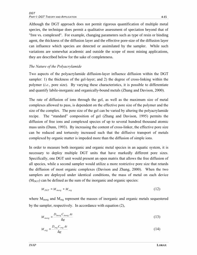
DGT PART I: DGT THEORY AND APPLICATION 4-15
INAP LORAX
Although the DGT approach does not permit rigorous quantification of multiple metal
species, the technique does permit a qualitative assessment of speciation beyond that of
"free vs. complexed". For example, changing parameters such as type of resin or binding
agent, the thickness of the diffusion layer and the effective pore-size of the diffusion layer
can influence which species are detected or assimilated by the sampler. While such
variations are somewhat academic and outside the scope of most mining applications,
they are described below for the sake of completeness.
The Nature of the Polyacrylamide
Two aspects of the polyacrylamide diffusion-layer influence diffusion within the DGT
sampler: 1) the thickness of the gel-layer; and 2) the degree of cross-linking within the
polymer (i.e., pore size). By varying these characteristics, it is possible to differentiate
and quantify labile-inorganic and organically-bound metals (Zhang and Davison, 2000).
The rate of diffusion of ions through the gel, as well as the maximum size of metal
complexes allowed to pass, is dependent on the effective pore size of the polymer and the
size of the complex. The pore size of the gel can be varied by altering the polyacrylamide
recipe. The “standard” composition of gel (Zhang and Davison, 1995) permits the
diffusion of free ions and complexed species of up to several hundred thousand atomic
mass units (Dunn, 1993). By increasing the content of cross-linker, the effective pore size
can be reduced and tortuosity increased such that the diffusive transport of metals
complexed by organic matter is impeded more than the diffusion of simple ions.
In order to measure both inorganic and organic metal species in an aquatic system, it is
necessary to deploy multiple DGT units that have markedly different pore sizes.
Specifically, one DGT unit would present an open matrix that allows the free diffusion of
all species, while a second sampler would utilize a more restrictive pore size that retards
the diffusion of most organic complexes (Davison and Zhang, 2000). When the two
samplers are deployed under identical conditions, the mass of metal on each device
(MDGT) can be defined as the sum of the inorganic and organic species:
orginorgDGT MMM += (12)
where Minorg and Morg represent the masses of inorganic and organic metals sequestered
by the sampler, respectively. In accordance with equation (2),
g
AtCDM
inorginorginorg ∆
= (13)
g
AtCDM
orgorgorg ∆
= (14)
DGT PART I: DGT THEORY AND APPLICATION 4-16
INAP LORAX
where Cinorg and Corg are the respective concentrations of labile inorganic and organic
metal complexes in solution. Equation (12) becomes:
g
AtCDCDM
orgorginorginorgDGT ∆
+=
)( (15)
Rearranging, equation (15) becomes:
inorginorg
orgorg
DGT CD
DC
At
gM+
=
∆)( (16)
Thus, plotting At
gM DGT ∆)( vs.
inorg
org
D
D
should produce a linear relationship in which the slope yields the concentration of organic
species (Corg), while the y-intercept represents the concentration of inorganic species
(Cinorg) (Zhang and Davison, 1999; 2000).
Thus, if the diffusion coefficient of the organic species is known, the total amount of
metal sequestered by the gel can be separated into a contribution from inorganic (rapidly-
diffusing) and organic (slowly-diffusing) fractions. This approach has resulted in
determinations of labile Cd concentrations that agree extremely well with independent
determinations by anodic stripping voltammetry (Zhang and Davison, 2000).
An alternative parameter that may be altered in the DGT sampler is the thickness of the
gel-layer. Since diffusive transport through the gel limits metal sequestration by the resin
to those complexes that can dissociate on the timescale of diffusion, metal-ligand
complexes with slow dissociation kinetics are largely undetected by the DGT approach.
It is therefore possible to alter the types of species which are assimilated by the sampler
by varying the thickness of this layer; a thinner gel-layer biases the sampler towards the
exclusion of progressively less labile metal species (Davison and Zhang, 2000).
The Nature of the Resin
While most applications of DGT have involved the use of Chelex 100, and hence have
focused on trace metals, it is possible in principle to use any one of a number of binding
agents in order to measure a variety of solutes. For example, certain exchange resins have
been used for 137
Cs and Sr (Davison et al., 2000 Chang et al., 1998). Cs, for example,
has been detected using ammonium molybdophosphate (AMP) as the binding agent
(Chang et al., 1998) and ferrihydrite has been used to fix phosphate (Zhang et al., 1998a;
1998b). Yet another application involves the use of silver iodide for the detection of free
sulphide (Teasdale et al., 1999; Teasdale, in press). Regardless of the specific binding
DGT PART I: DGT THEORY AND APPLICATION 4-17
INAP LORAX
agent utilized, all approaches rely on molecular diffusion of labile species through the gel
layer to quantify solute uptake.
4.3.2 Toxicity
Several investigations have demonstrated that DGT provides a quantitative measure of
labile (free or kinetically-labile) metal species in aquatic systems (e.g., McNee and
Martin, 1999). Given that the toxicity of many metals (e.g., Cu, Ni, Cd, Pb) has been
shown to be a function of the free-ion activity (see Chapter 2), it is possible that that DGT
provides a more representative indicator of bioavailability, and hence, toxicity than assays
of total dissolved metal concentration. However, few data currently exist which directly
compare measurements of DGT and toxicity to aquatic biota. In the following section,
the results from a series of experiments conducted by Lorax are presented which relate
metal toxicity to the metal fraction as defined by DGT. Specifically, experiments were
conducted in which various test organisms (Daphnia magna and rainbow trout) were
exposed to varying concentrations of dissolved copper, both in the presence and absence
of copper complexing agents (ligands). Both synthetic and natural ligands were used. In
each experiment, both DGT-Cu and dissolved Cu were determined. In this manner,
toxicity measured via standard LC50 approaches could be compared with both dissolved
and DGT-inferred metal concentrations.
Experiments using the synthetic ligand EDTA (ethylenediaminetetraacetic acid) were
conducted with both D. magna and rainbow trout (Salmo gairdneri). In experiments with
D. magna, forty-eight-hour bioassays were carried out with dissolved Cu concentrations
ranging from 0 to ~500 µg/L, both with and without a 7-fold molar excess of EDTA
(Figure 4-6). The respective concentrations were chosen to bracket the range of dissolved
Cu levels encountered in contaminated waters, and to illustrate clearly the applicability of
DGT in estimations of bioavailability in the presence of significant concentrations of
complexing ligands. In the absence of EDTA, dissolved and DGT-inferred Cu
concentrations generally agreed within 10%, indicating that in the absence of metal-
complexing ligands, the DGT technique is capable of reasonably precise quantification of
the dissolved Cu concentration (Figure 4-6a). With no EDTA added, daphnid survival
decreased with increasing Cu concentrations; the LC50 was calculated to be ~12 µg/L
(Figure 4-6b). Conversely, in the presence of excess EDTA, DGT-inferred concentrations
were significantly reduced in comparison to the total dissolved fraction (Figure 4-6a).
Such observations reflect the strength of Cu-EDTA complexes and lack of sorption of
such species by the DGT device. In the presence of EDTA, D. magna exhibited 100%
survival at all dissolved Cu concentrations, indicating that Cu-EDTA complexes were
also unavailable to the test species (Figure 4-6b).

DGT PART I: DGT THEORY AND APPLICATION 4-18
INAP LORAX
0
20
40
60
80
100
120
0 100 200 300 400 500
no EDTAwith EDTA
%su
rviv
al
D isso lved [Cu] (µ g/L)
LC5 0
Daphnia magnaB
0
100
200
300
400
500
0 100 200 300 400 500
no ED T A
w ith ED T A
DG
T [
Cu
] (µ
g/L
)
D issolved [Cu] Added (µg /L)
1:1
A
Figure 4-6: Daphnia magna 48 h bioassay: a) Copper concentrations determined by DGT vs. dissolved concentrations, for solutions with no EDTA and with a seven-fold molar excess of EDTA. The dashed lines represent 10% error boundary in 1:1 slope; b) percent survival in test cultures of Daphnia magna vs. dissolved Cu concentration for solutions without added EDTA and with a seven-fold molar excess of EDTA. Estimate of LC50 is represented by the shaded area (Lorax, unpublished data). For both a and b, test solutions (pH = 7.5) consisted of moderately hard (100 mg/L as CaCO3), Chelex-cleaned reconstituted fresh water and was prepared by adding 96 mg/L NaHCO3, 60 mg/L CaSO4
.2H2O, 60 mg/L MgSO4, and 4.0 mg/L KCl .
DGT PART I: DGT THEORY AND APPLICATION 4-19
INAP LORAX
Similar to the daphnid experiment, bioassays using rainbow trout were carried out with
dissolved Cu concentrations ranging from 0 to ~500 µg/L, both with and without a 7-fold
molar excess of EDTA (Figure 4-7). As for the daphnid bioassay, dissolved and DGT-
inferred Cu concentrations exhibited a near 1:1 relationship in the absence of EDTA
(Figure 4-7a). With no EDTA, trout mortality increased progressively with the amount of
Cu added; the LC50 was 53 µg/L (Figure 4-7b). In the presence of excess EDTA, DGT-
inferred Cu concentrations were significantly reduced (Figure 4-7a); trout exhibited 100%
survival throughout the entire concentration range (Figure 4-7b). The results are
consistent with the daphnid experiment, and indicate that Cu-EDTA complexes are
largely unavailable to both DGT and aquatic biota. In other words, the concentration of
“available” metal recorded using the DGT approach is consistent with the “available-
metal” moiety assimilated by the aquatic organisms used in the Lorax experiments.
Experiments using natural ligands were conducted with waters collected from the
Nicomekl River (Figure 4-8; Lorax, unpublished data), a meandering watercourse that
drains low-relief marshland regions of the Fraser River delta, near Vancouver, B.C. The
waters are heavily stained, and contain abundant DOC(~8 mg/L). Forty-eight-hour
bioassays with D. magna were conducted using Nicomekl River water to which was
added dissolved Cu concentrations ranging from 0 to 220 µg/L. As a control, identical
bioassays were conducted in Nicomekl-free growth medium (Chelex-cleaned,
reconstituted moderately hard freshwater as described in Figure 4-6) with Cu
concentrations ranging from 0 to ~50 µg/L. In the absence of Nicomekl water (i.e.,
growth medium only), dissolved and DGT-inferred Cu concentrations agreed to within
~10%, demonstrating that all of the Cu added was in a labile form (Figure 4-8a). In this
ligand-free scenario, the LC50 was determined to occur at a dissolved Cu concentration of
10.8 µg/L (Figure 4-8b). In the presence of DOC-rich Nicomekl River water, DGT-
inferred Cu concentrations were significantly reduced (Figure 4-8a). The reduction of
DGT-inferred Cu by roughly a factor of two reflects the formation of Cu-organic
complexes which are not sequestered as readily by the DGT device in comparison to the
free metal ion (Figure 4-8a). Cu bound to organic matter will also diffuse more slowly
than inorganic complexes of Cu or free ion, further reducing the sequestration of the
metal by the gel-resin. Toxicity towards daphnids in Nicomekl River waters was reduced
considerably in comparison to the growth medium. D. magna exhibited 100% survival at
dissolved Cu concentrations up to ~100 µg/L, decreasing to 0% survival at a
concentration of 210 µg/L (Figure 4-8b). The corresponding LC50 was calculated to occur
at a dissolved Cu concentration of 170±20 µg/L. Such enhanced survival is consistent
with the reduction in the concentration of labile-Cu in the river medium as determined by
DGT.
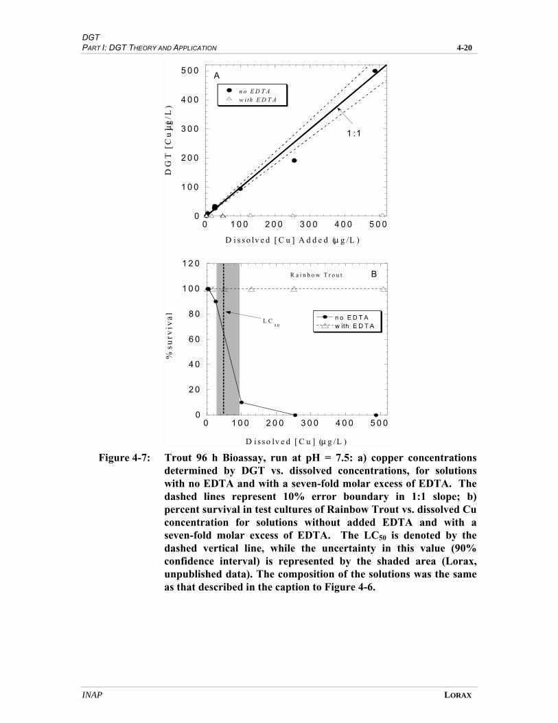
DGT PART I: DGT THEORY AND APPLICATION 4-20
INAP LORAX
0
2 0
4 0
6 0
8 0
1 0 0
1 2 0
0 1 0 0 2 0 0 3 0 0 4 0 0 5 0 0
n o E D T Aw ith E D T A
%s
urv
iv
al
D i s s o lv e d [ C u ] (µ g /L )
L C5 0
R a i n b o w T r o u t B
0
1 0 0
2 0 0
3 0 0
4 0 0
5 0 0
0 1 0 0 2 0 0 3 0 0 4 0 0 5 0 0
n o E D T Aw ith E D T A
DG
T [
Cu
] (µg
/L
)
D i s s o lv e d [ C u ] A d d e d (µ g /L )
1 :1
A
Figure 4-7: Trout 96 h Bioassay, run at pH = 7.5: a) copper concentrations
determined by DGT vs. dissolved concentrations, for solutions with no EDTA and with a seven-fold molar excess of EDTA. The dashed lines represent 10% error boundary in 1:1 slope; b) percent survival in test cultures of Rainbow Trout vs. dissolved Cu concentration for solutions without added EDTA and with a seven-fold molar excess of EDTA. The LC50 is denoted by the dashed vertical line, while the uncertainty in this value (90% confidence interval) is represented by the shaded area (Lorax, unpublished data). The composition of the solutions was the same as that described in the caption to Figure 4-6.
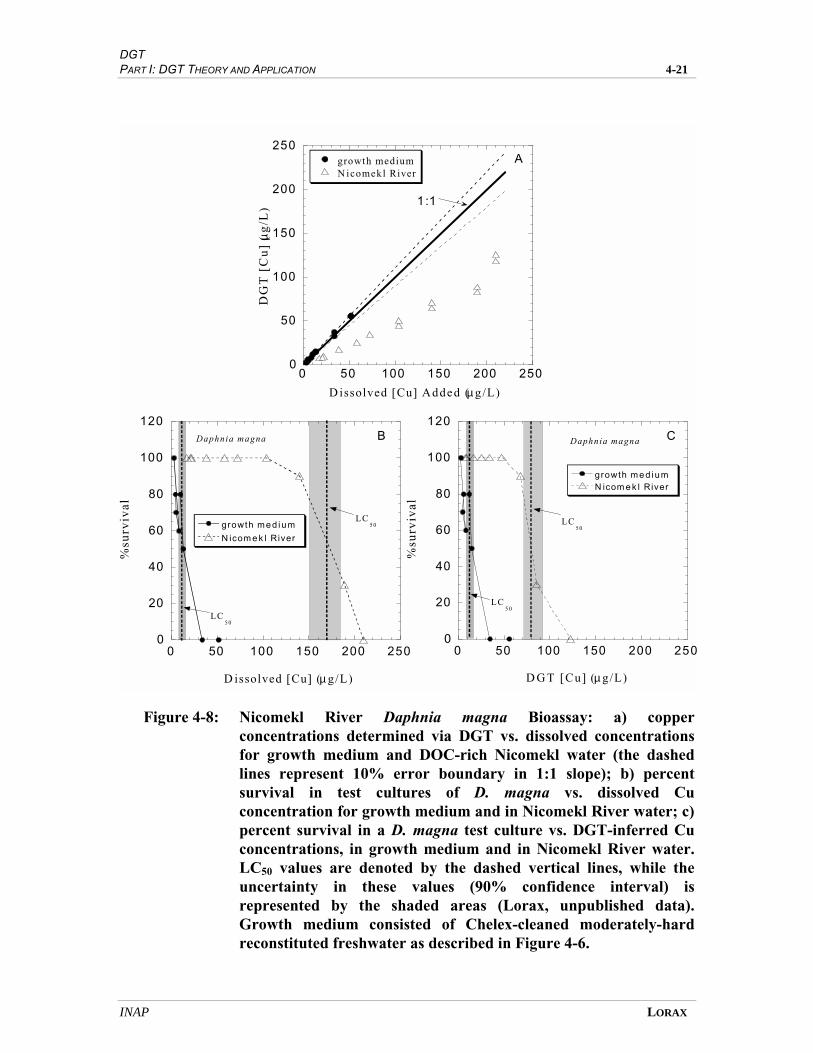
DGT PART I: DGT THEORY AND APPLICATION 4-21
INAP LORAX
0
20
40
60
80
100
120
0 50 100 150 200 250
growth med ium
N icom e k l River
%su
rv
iva
l
D issolved [Cu] (µ g/L)
LC50
LC50
Daphnia magna B
0
50
100
150
200
250
0 50 100 150 200 250
growth medium
N icomekl River
DG
T [
Cu
] (µ
g/L
)
D issolved [Cu] Added (µ g /L)
1:1
A
0
20
40
60
80
100
120
0 50 100 150 200 250
growth med iumN icom e k l River
%su
rviv
al
D G T [Cu] (µ g/L)
LC50
LC5 0
Daphnia magna C
Figure 4-8: Nicomekl River Daphnia magna Bioassay: a) copper concentrations determined via DGT vs. dissolved concentrations for growth medium and DOC-rich Nicomekl water (the dashed lines represent 10% error boundary in 1:1 slope); b) percent survival in test cultures of D. magna vs. dissolved Cu concentration for growth medium and in Nicomekl River water; c) percent survival in a D. magna test culture vs. DGT-inferred Cu concentrations, in growth medium and in Nicomekl River water. LC50 values are denoted by the dashed vertical lines, while the uncertainty in these values (90% confidence interval) is represented by the shaded areas (Lorax, unpublished data). Growth medium consisted of Chelex-cleaned moderately-hard reconstituted freshwater as described in Figure 4-6.
DGT PART I: DGT THEORY AND APPLICATION 4-22
INAP LORAX
The DGT-inferred concentrations at which mortality occurred in the river waters were
significantly higher than the levels at which mortality occurred in the absence of added
ligands (Figure 4-8c); the LC50 in the river medium (DGT-Cu = 80 µg/L) was
approximately 7 times greater than that calculated for the growth medium
(DGT-Cu = 11 µg/L). Such observations imply that DGT sequesters some metal species
that are unavailable to aquatic biota, i.e. labile species, not just free ion. In this example,
therefore, DGT provides a conservative estimate of toxicity.
In summary, the DGT/bioassay experiments suggest that DGT provides a more
representative measure of metal bioavailability, and hence toxicity, than conventional
measurements of dissolved species. Specifically, the results indicate that metal uptake by
DGT and aquatic biota is reduced in the presence of metal-complexing ligands. The
results also highlight the limited utility of total and total dissolved Cu concentrations as a
proxy for the bioavailable fraction in waters that contain significant concentrations of Cu-
complexing ligands.
4.3.3 Kinetics of Complexation
The principal application of DGT in environmental studies has been its use as an in situ
tool for assessing metal speciation in aquatic systems. As outlined above, DGT provides
a general measure of the biologically available, or "labile" concentration of metals in
solution. In addition to speciation measurements, DGT may also be used to examine the
kinetics (i.e., rate) of metal-ligand complexation. When a metal is added to a solution
containing metal-complexing ligands, the concentration of free-metal ion will
progressively decrease until an equilibrium is established between ion and ligand. Since
DGT provides a measure of the labile-metal concentration, the rate at which this fraction
decreases can be used to quantify the rate of the association reaction. Kinetic
considerations have considerable relevance to predictions of metal toxicity in receiving
waters into which mining-related effluents are discharged. The following section
discusses the applicability of DGT to studies of metal-ligand complexation kinetics, with
emphasis on the application to the mining industry. The discussion is supported by
experimental data acquired by Lorax.
Metal speciation in natural waters varies markedly, and is affected by several variables
including the types and concentrations of metals and ligands present, salinity, pH, pE,
biological processes, particle concentration, etc. Accordingly, the speciation of metals
originating from mining-related sources will respond to the specific physical and
chemical conditions of the receiving waters. The “free ion” concentration (and hence,
toxicity, according to the Free Ion Activity Model (Campbell, 1995) can be significantly
reduced, for example, when ligands (e.g., dissolved organics) are present in excess of the
metal concentrations. Given the importance of metal speciation in determining toxicity,

DGT PART I: DGT THEORY AND APPLICATION 4-23
INAP LORAX
an understanding of the former is fundamental to establishing more accurate estimates of
assimilative capacity, which can be used to develop site-specific discharge criteria. In
this respect, an important consideration is the rate at which uncomplexed (and potentially
toxic) metals in effluent are transformed into complexed (less toxic) metal by the ligands
in the receiving waters. While thermodynamic data provide information with respect to
tendency of a reaction to occur, kinetics dictate the rate of metal-ligand reactions. Kinetic
considerations have particular relevance to the discharge of mining-related effluents, the
toxicity of which may vary over time and space (e.g., downstream) in the receiving
environment. This is particularly important for metals such as Ni, which are
characterized by slow complexation kinetics (Bedsworth and Sedlak, 1999).
In order to demonstrate the ability of DGT to assess the kinetics of metal complexation,
two experiments were conducted with mine effluent (Lorax, unpublished data). In the
first experiment, a synthetic ligand (EDTA) was added in varying concentrations to the
mine effluent and the DGT-Ni fraction measured after 24 h and 14 days. The EDTA was
added such that a "free metal " gradient was established, with progressively less free
metal available with increasing EDTA concentration. Measured DGT-Ni concentrations
were compared to those predicted assuming instantaneous equilibrium between EDTA
and the metals present. Inspection of the results indicates that one day after EDTA
addition, DGT-inferred Ni concentrations were significantly higher than the predicted
equilibrium values (Figure 4-9). Although there is little difference between predicted and
observed (by DGT) values at [EDTA] < 1 mg/L, the DGT-Ni value of ~36 µg/L observed
at an EDTA concentration of 3 mg/L is over two orders of magnitude greater than the
predicted value. Similarly, at [EDTA] = 10 mg/L, the predicted [Ni]free is far lower than
that assayed by DGT. In contrast, the DGT-inferred Ni concentrations after 14 days were
much closer to the levels “predicted” (Figure 4-9). The DGT results demonstrate the
apparent importance of Ni-ligand exchange kinetics with EDTA.
In the second experiment, a range of EDTA concentrations was added to mine effluent
and the DGT-inferred concentrations determined in all solutions after a 24-hour
incubation period. In this manner, the time-dependence of DGT-inferred Ni
concentration could be modelled as a function of the EDTA concentration, assuming first-
order reaction kinetics. Such modelling provides evidence of slow reaction kinetics for
the formation of Ni-EDTA complexes (Figure 4-10). With increasing concentrations of
EDTA, DGT-inferred Ni concentrations decrease gradually and non-linearly from a value
equal to the dissolved concentration (~65 mg/L) at no EDTA to a minimum of ~3 µg/L in
the presence of 18 mg/L EDTA (Figure 4-10). The non-linearity of the response curve
suggests that the rate of Ni-EDTA complex formation is kinetically controlled, and
follows first-order kinetics . Specifically, Ni-EDTA complex formation is faster at higher
concentrations of EDTA, with the concentration of uncomplexed Ni (i.e., DGT-inferred)

DGT PART I: DGT THEORY AND APPLICATION 4-24
INAP LORAX
0
10
20
30
40
50
60
70
0 2 4 6 8 10
After 1 Day
dissolvedDGTpred. equilibriumfree ion
Ni (
µg
/L)
EDTA (mg/L)
0
10
20
30
40
50
60
70
0 2 4 6 8 10
After 14 Days
dissolvedDGTpred. equilibriumfree ion
Ni (
µg
/L)
EDTA (mg/L) Figure 4-9: Dissolved, DGT-inferred and predicted (at equilibrium) Ni
concentrations in mine effluent, 1 and 14 d after addition of EDTA. The mine effluent consisted of circumneutral pH tailings pond overflow. Predicted Ni concentrations represent those based on thermodynamic equilibria.
increasing with decreasing EDTA concentration (Figure 4-10). If kinetics were not
important (i.e., assuming an instantaneous reaction), the concentration of DGT-inferred
Ni would decrease linearly with increasing EDTA concentration to values <0.1 µg/L.
Thus, although Ni-EDTA complexes are very strong, the kinetics of formation appear to
be slow, with complete equilibration requiring days to weeks. Such observations have
been reported elsewhere (Bedsworth and Sedlak, 1999; Hudson, 1998).

DGT PART I: DGT THEORY AND APPLICATION 4-25
INAP LORAX
0
10
20
30
40
50
60
70
0 5 10 15 20
measured by DGTmodelled
[DG
T N
i],
µg
/L
[EDTA] mg/L
Figure 4-10: Measured “DGT”-Ni and modelled “free”-Ni as a function of EDTA concentration. Measured values represent the DGT fraction after a 24 h incubation period with EDTA. The model assumes complexation occurring for 24 hours according to first-order kinetics with a Ni complexation rate constant that is directly proportional to the EDTA concentration. Note that the precise rate law for Ni-EDTA complex formation is not known, but first-order reaction kinetics are likely.
In summary, the results suggest that DGT offers potential to assess the kinetics of
formation of metal-ligand complexes. The experimental results also indicate that
speciation (and hence toxicity) cannot be predicted from equilibrium considerations
alone. This DGT application has several potential applications in the mining sector. For
example, at sites which discharge effluent to receiving waters, an understanding of how
rapidly introduced metals interact with natural ligands could aid in:
1. determination of effluent toxicity over time;
2. assessment of effluent toxicity with distance downstream of the discharge point;
3. the development of site specific discharge limits;
4. determining the time interval required for effluent treatment processing before
discharge to the environment. EDTA, for example, may be added to effluent process
streams to reduce the bioavailability (i.e., toxicity) of the final discharge. Given the
slow reaction kinetics of some metals with EDTA (e.g., Ni), a sufficient time period
is necessary to ensure equilibration; and
DGT PART I: DGT THEORY AND APPLICATION 4-26
INAP LORAX
5. validating toxicity tests outlined by regulatory bodies (e.g., MISA). For example,
systems which exhibit slow reaction kinetics between metals and ligands in
receiving waters may yield differing LC50 values depending on the time period
between sample collection and toxicity tests. The kinetics of metal complexation
will dictate the rate at which toxicity is ameliorated, and thus, will aid in
determining most appropriate time interval in which to conduct toxicity tests.
4.3.4 Complexation Capacity
The ability of an aquatic system to complex metals in solution (i.e., complexation
capacity) if often used in environmental impact studies to assess the assimilative capacity
of receiving waters (Carter et al., 1992; Pardo et al., 1994; Yang et al., 1999). It is
commonly accepted that in the presence of complexing agents (most commonly dissolved
organic matter), metal toxicity is ameliorated, and thus the assimilative capacity of the
receiving environment is enhanced. Furthermore, it is also understood that the degree to
which toxicity abatement takes place depends largely on the quantity and type of organic
matter in receiving waters. Accordingly, estimates of assimilative capacity are sometimes
made in which a metal-specific complexing capacity is assigned to a receiving water
body; that value is then applied to adjust receiving-water criteria. Unfortunately, the
notion of complexing capacity is often misunderstood to the degree that a measured value
is broadly used to adjust receiving-water criteria without regard to considerations of both
ligand concentration and ligand affinity.
There are two salient considerations in regards to the degree of metal complexation: 1)
the concentration of the ligands present; and 2) the ligand binding strength for the metal
of interest. For example, a large concentration of a weak or intermediate-strength ligand
(i.e., one that allows a significant fraction of free metal in solution) is often less effective
at ameliorating toxicity than a low concentration of a strong ligand. Figure 4-11
illustrates this notion with three hypothetical cases: no ligand/weak ligand, a ligand of
intermediate strength, and a strong ligand. The plot is a representation of “free” metal
concentration as a function of incremental metal additions to the ligand-containing
solution. In the case of no ligand or a weak ligand, all of the metal added to solution is
accounted for in the “free” metal inventory. “Free” metal is used here to connote
organically-uncomplexed ions, but may include hydroxo-complexes. Given this caveat,
there is no effective complexing capacity and the slope of the data regression is unity (i.e.,
1:1). In the case of an intermediate ligand, only a fraction of the added metal can be
allocated to the free inventory. Once all ligand sites are saturated (the break in the slope;
Figure 4-11), the adsorption capacity is exceeded and any additional metal is
quantitatively added to the free inventory (i.e., the slope of the line adopts a 1:1 slope at
dissolved M2+
values >~180 µg/L). In the strong ligand case, very little of the added
metal occurs in the free pool until all sites are saturated, at which point any additional
metal is quantitatively added to the free inventory.
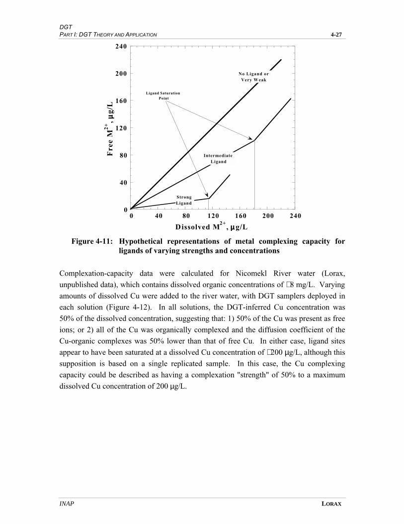
DGT PART I: DGT THEORY AND APPLICATION 4-27
INAP LORAX
0
40
80
120
160
200
240
0 40 80 120 160 200 240
Fre
e M
2+, µµ
g/L
D issolved M2+
, µµ g/L
No Ligand orVery W eak
IntermediateLigand
StrongLigand
Ligand SaturationPoint
Figure 4-11: Hypothetical representations of metal complexing capacity for ligands of varying strengths and concentrations
Complexation-capacity data were calculated for Nicomekl River water (Lorax,
unpublished data), which contains dissolved organic concentrations of ∼ 8 mg/L. Varying
amounts of dissolved Cu were added to the river water, with DGT samplers deployed in
each solution (Figure 4-12). In all solutions, the DGT-inferred Cu concentration was
50% of the dissolved concentration, suggesting that: 1) 50% of the Cu was present as free
ions; or 2) all of the Cu was organically complexed and the diffusion coefficient of the
Cu-organic complexes was 50% lower than that of free Cu. In either case, ligand sites
appear to have been saturated at a dissolved Cu concentration of ∼ 200 µg/L, although this
supposition is based on a single replicated sample. In this case, the Cu complexing
capacity could be described as having a complexation "strength" of 50% to a maximum
dissolved Cu concentration of 200 µg/L.
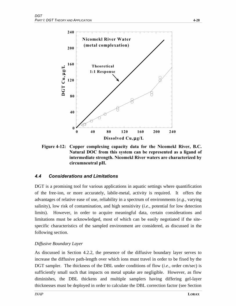
DGT PART I: DGT THEORY AND APPLICATION 4-28
INAP LORAX
0
40
80
120
160
200
240
0 40 80 120 160 200 240
Nicomekl River Water(metal complexation)
DG
T C
u, µµ
g/L
Dissolved Cu, µµg/L
Theoretical1:1 Response
Figure 4-12: Copper complexing capacity data for the Nicomekl River, B.C. Natural DOC from this system can be represented as a ligand of intermediate strength. Nicomekl River waters are characterized by circumneutral pH.
4.4 Considerations and Limitations
DGT is a promising tool for various applications in aquatic settings where quantification
of the free-ion, or more accurately, labile-metal, activity is required. It offers the
advantages of relative ease of use, reliability in a spectrum of environments (e.g., varying
salinity), low risk of contamination, and high sensitivity (i.e., potential for low detection
limits). However, in order to acquire meaningful data, certain considerations and
limitations must be acknowledged, most of which can be easily negotiated if the site-
specific characteristics of the sampled environment are considered, as discussed in the
following section.
Diffusive Boundary Layer
As discussed in Section 4.2.2, the presence of the diffusive boundary layer serves to
increase the diffusive path-length over which ions must travel in order to be fixed by the
DGT sampler. The thickness of the DBL under conditions of flow (i.e., order cm/sec) is
sufficiently small such that impacts on metal uptake are negligible. However, as flow
diminishes, the DBL thickens and multiple samplers having differing gel-layer
thicknesses must be deployed in order to calculate the DBL correction factor (see Section
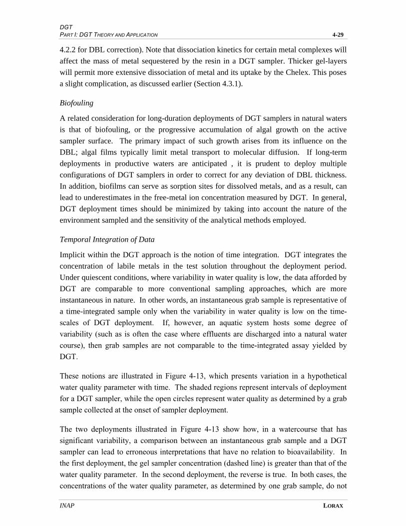
DGT PART I: DGT THEORY AND APPLICATION 4-29
INAP LORAX
4.2.2 for DBL correction). Note that dissociation kinetics for certain metal complexes will
affect the mass of metal sequestered by the resin in a DGT sampler. Thicker gel-layers
will permit more extensive dissociation of metal and its uptake by the Chelex. This poses
a slight complication, as discussed earlier (Section 4.3.1).
Biofouling
A related consideration for long-duration deployments of DGT samplers in natural waters
is that of biofouling, or the progressive accumulation of algal growth on the active
sampler surface. The primary impact of such growth arises from its influence on the
DBL; algal films typically limit metal transport to molecular diffusion. If long-term
deployments in productive waters are anticipated , it is prudent to deploy multiple
configurations of DGT samplers in order to correct for any deviation of DBL thickness.
In addition, biofilms can serve as sorption sites for dissolved metals, and as a result, can
lead to underestimates in the free-metal ion concentration measured by DGT. In general,
DGT deployment times should be minimized by taking into account the nature of the
environment sampled and the sensitivity of the analytical methods employed.
Temporal Integration of Data
Implicit within the DGT approach is the notion of time integration. DGT integrates the
concentration of labile metals in the test solution throughout the deployment period.
Under quiescent conditions, where variability in water quality is low, the data afforded by
DGT are comparable to more conventional sampling approaches, which are more
instantaneous in nature. In other words, an instantaneous grab sample is representative of
a time-integrated sample only when the variability in water quality is low on the time-
scales of DGT deployment. If, however, an aquatic system hosts some degree of
variability (such as is often the case where effluents are discharged into a natural water
course), then grab samples are not comparable to the time-integrated assay yielded by
DGT.
These notions are illustrated in Figure 4-13, which presents variation in a hypothetical
water quality parameter with time. The shaded regions represent intervals of deployment
for a DGT sampler, while the open circles represent water quality as determined by a grab
sample collected at the onset of sampler deployment.
The two deployments illustrated in Figure 4-13 show how, in a watercourse that has
significant variability, a comparison between an instantaneous grab sample and a DGT
sampler can lead to erroneous interpretations that have no relation to bioavailability. In
the first deployment, the gel sampler concentration (dashed line) is greater than that of the
water quality parameter. In the second deployment, the reverse is true. In both cases, the
concentrations of the water quality parameter, as determined by one grab sample, do not
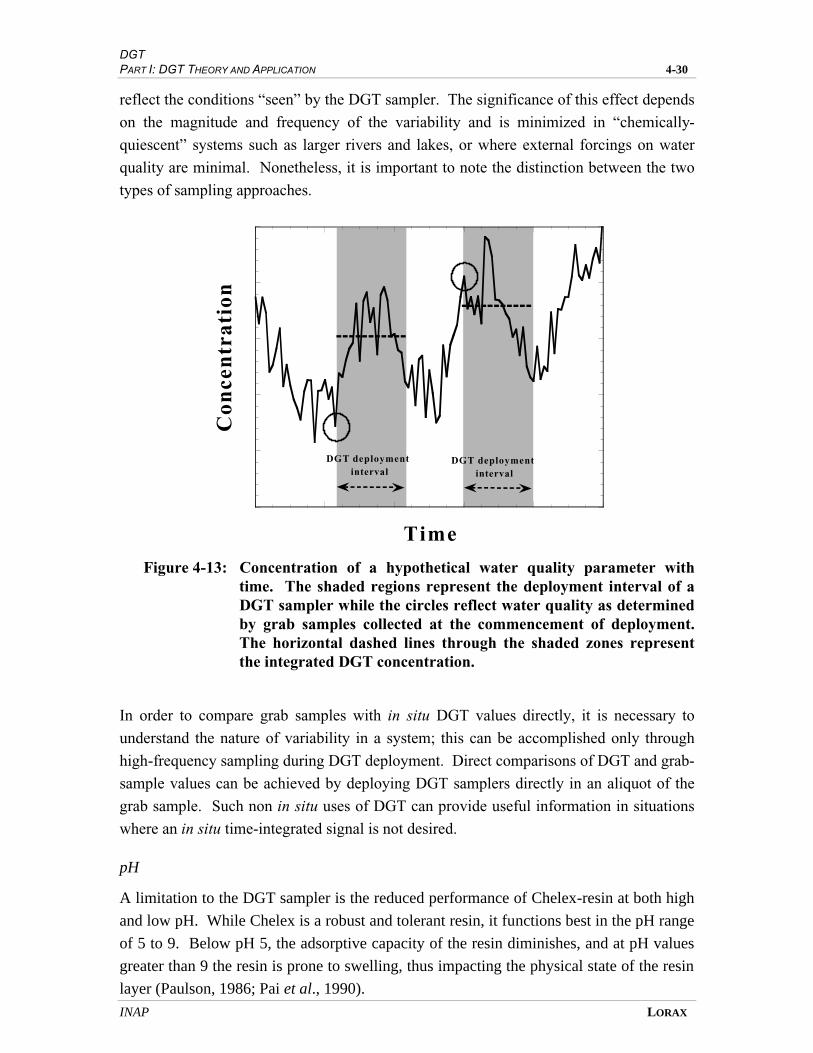
DGT PART I: DGT THEORY AND APPLICATION 4-30
INAP LORAX
reflect the conditions “seen” by the DGT sampler. The significance of this effect depends
on the magnitude and frequency of the variability and is minimized in “chemically-
quiescent” systems such as larger rivers and lakes, or where external forcings on water
quality are minimal. Nonetheless, it is important to note the distinction between the two
types of sampling approaches.
Con
cen
trat
ion
Time
DGT deploymentinterval
DGT deploymentinterval
Figure 4-13: Concentration of a hypothetical water quality parameter with time. The shaded regions represent the deployment interval of a DGT sampler while the circles reflect water quality as determined by grab samples collected at the commencement of deployment. The horizontal dashed lines through the shaded zones represent the integrated DGT concentration.
In order to compare grab samples with in situ DGT values directly, it is necessary to
understand the nature of variability in a system; this can be accomplished only through
high-frequency sampling during DGT deployment. Direct comparisons of DGT and grab-
sample values can be achieved by deploying DGT samplers directly in an aliquot of the
grab sample. Such non in situ uses of DGT can provide useful information in situations
where an in situ time-integrated signal is not desired.
pH
A limitation to the DGT sampler is the reduced performance of Chelex-resin at both high
and low pH. While Chelex is a robust and tolerant resin, it functions best in the pH range
of 5 to 9. Below pH 5, the adsorptive capacity of the resin diminishes, and at pH values
greater than 9 the resin is prone to swelling, thus impacting the physical state of the resin
layer (Paulson, 1986; Pai et al., 1990).
DGT PART I: DGT THEORY AND APPLICATION 4-31
INAP LORAX
Saturation of Complexing Capacity of Resin
The mass of Chelex resin contained within the metal-binding gel layer affords
considerable complexation capacity for sorbed metals. However, the complexation
capacity of the resin layer is finite. Thus, given a large enough inventory of metals in
solution and sufficient deployment period, saturation of the resin will occur. The time to
reach saturation will vary greatly, depending on the metals present in solution, metal
concentration, temperature and thickness of the diffusion layer. Limitations of resin
saturation can be easily overcome as long as site-specific factors are considered when
determining appropriate deployment periods.
Low Ionic Strength Solutions
Recent research suggests that DGT may overestimate the labile metal fraction in low
ionic-strength solutions (Alfaro-De la Torre et al., 2000). Specifically, in solutions that
contain major ion concentrations < 2 x 10⁻⁴
M, concentrations of Cd and Ni measured by
DGT were consistently higher than comparable total dissolved measurements. Such
observations were attributed to an increase in metal diffusion coefficients associated with
electrical effects induced by charge imbalances across the diffusive layer. The results
have implications with respect to the use of DGT in low ionic strength media (e.g.,
pristine, soft-water lakes). However, additional research is required to quantify more
precisely the effects of such processes.
Ineffectiveness of DGT for Some Metals/Metalloids
DGT in its present form (i.e., Chelex resin) is capable of measuring the labile
concentration of a wide spectrum of trace metals in aquatic systems. Many metal cations
(e.g., Cu, Ni, Zn, Fe, Pb) exhibit a strong affinity for Chelex exchange sites. Chelex is
limited, however, with respect to metals which commonly exist as oxyanions in solution
(e.g., As, Mo, Se, Sb) and which may not be preferentially adsorbed by the resin (Pai et
al., 1990). Such constraints are at worst short-term limitations, however, and will be
rectified with the incorporation of alternative resins (e.g., anionic exchange resins).
Indeed, species-specific DGT applications have already been developed for Cs, Sr, H2S
and PO43-
.
Limitations of Free-Ion Activity Model
The parallels between metal uptake by DGT and aquatic biota relate to the Free-Ion
Activity Model (FIAM) (see Chapter 2); uptake is related to the concentration of free and
kinetically-labile metals in solution. The general similarity in uptake mechanisms
explains why DGT appears to provide a better proxy of bioavailability than other
traditional measurements of dissolved or total metals. However, there are exceptions to
the FIAM which apply to DGT. Some non-polar neutrally-charged species (e.g., AgCl,
DGT PART I: DGT THEORY AND APPLICATION 4-32
INAP LORAX
HgCl2), for example, are lipid-soluble, and as a result, are able to diffuse freely across
cellular membranes. In this manner, metal uptake occurs in the absence of metal binding
to transmembrane transporters (Gutknecht, 1981; Phinney and Bruland, 1994). The
presence of synthetic organic ligands (e.g., dithiocarbamate, 8-hydroxyquinoline) and low
molecular-weight ligands (e.g., citrate) has also been shown to increase the cellular
uptake of several trace metals (see Chapter 2). The uptake of these aforementioned
species by DGT may also be constrained, although DGT will measure neutral complexes
if they are labile.
Another factor worthy of consideration is water hardness. The toxicity of metals to
aquatic organisms, for example, generally decreases with increasing water hardness (i.e.,
increasing concentrations of Ca and Mg) (see Chapter 2). Accordingly, in solutions of
varying water hardness, the activity of free metal ions may remain constant while the
toxicity towards aquatic biota may vary. This limitation of the FIAM also has
implications with respect to the use of DGT.
4.5 Data Gaps and Future Research
The application of DGT to studies of metal speciation in aquatic systems has advanced
considerably since its relatively-recent implementation. DGT techniques can be applied to
explore various aspects of environmental chemistry in various test media (e.g., water,
sediments and soils). However, further research is necessary to rigourously defend
interpretations inferred from DGT measurements in varying environments. In particular,
the application of this technique to mining-impacted systems requires further
examination. A summary of data gaps and future research is briefly highlighted below.
• More work is required to assess the precise nature of species measured by DGT in
various aquatic environments. In particular, attention should be given to the effects
of ligand competition with Chelex, size exclusion (i.e., polyacrylamide pore-size),
and differential diffusion of inorganic vs. organic species. Assessments of the metal
species measured by DGT, therefore, require rigorous comparison with other
speciation techniques (e.g., ASV, AdCSV, SLM; see Chapter 3).
• The relationship between DGT values and toxicity to aquatic biota requires further
study. The link between DGT and toxicity has been briefly examined with respect to
copper via comparisons of DGT-Cu concentrations and LC50 values as determined by
bioassay methods (see Section 4.3.2). However, this topic requires additional study,
and should be expanded to include other metals of environmental concern (e.g., Zn,
Cd, Ni, Pb, etc.).
DGT PART I: DGT THEORY AND APPLICATION 4-33
INAP LORAX
• Mining-related effluents present complex solutions hosting a spectrum of organic and
inorganic agents which have the potential to complex trace metals, thereby
influencing metal bioavailability and toxicity. Considerable work, therefore, is
needed to assess the utility of DGT in systems influenced by mining-related
discharges, and to determine how DGT values vary in response to the presence of
different ligands. In particular, cyanide compounds represent ubiquitous components
of most gold-mine waste streams and form strong complexes with many metals. The
interactions between metal-CN complexes and Chelex are poorly constrained, and
thus require examination. Mine-site discharges are also host to a variety of organic
reagents (e.g., pine oil, cresol, alcohols, xanthates, etc.) which undoubtedly influence
metal uptake by DGT.
International Network for Acid Preventi
5 DGT Sediment Probe
5-1
5. DGT Sediment Probe
5.1 Introduction
In this section, the theory and design of the DGT sediment probe are described and its
applicability to mining-related environmental studies is discussed. Although the scope of
the INAP project is focused on the DGT water sampler, a literature review was also
conducted on the DGT sediment probe and is included for completeness. The DGT
sediment probe may be utilized in sediment toxicity and sediment/tailings reactivity
assessments.
The principles of metal speciation and its affect on bioavailability and toxicity have been
described in Chapters 2 and 3. These concepts also apply to pore waters, where the
biological response (bioavailability) is suggested to be proportional to the free metal ion
activity in pore solution. Bioavailability of metals in pore waters can therefore be
decreased by complexation of metals by soluble inorganic (e.g., F-, Cl-, HCO3
-, SO4
2-,
HPO4
2-, HS-, polysulphides etc.) and organic (e.g., humic substances) ligands. In addition,
metal-binding phases in sediments (e.g., sulphides, particulate organic matter and iron
and manganese oxyhydroxides), may release “exchangeable” metals to pore waters.
Where steady-state conditions may exist, chemical equilibrium is established between the
solid phase and adjacent pore waters, with the concentration and speciation of metals in
pore waters being controlled by pore water chemistry (i.e., redox state, pH, ligands, etc.).
Accordingly, the DGT sediment probe may be used to assess labile metal concentrations
in pore waters or to determine the flux of exchangeable metals remobilized from the solid
phase. A complication in the application of the sediment probe is that organisms may not
“see” the same pore water as the probe. This is because many benthic organisms create
their own microenvironments (see, for example , Warren et al., 1998, and Hare et al.,
2001), often by irrigating their burrow with oxic water drawn from above. Thus, caution
must be used in assessments of pore-water toxicity as they relate to specific groups of
benthic organisms.
Following this brief introduction, existing techniques for conducting sediment toxicity
and sediment reactivity assessments are reviewed (Section 5.2). The theory and
application of the DGT sediment probe (Section 5.3) and a brief summary (Section 5.4)
are then presented.

DGT SEDIMENT PROBE PART I: DGT THEORY AND APPLICATION 5-2
INAP LORAX
5.2 Existing Techniques for Assessing Sediment Geochemistry and Toxicity
Currently, there are several established techniques available for assessing the subaqueous
chemical reactivity of sediment/tailings and sediment toxicity. Descriptions of such
methods are outlined in the following sections.
5.2.1 Sediment/Tailings Reactivity Assessment
Previous assessments of the post-depositional cycling of metals in contaminated
sediments and submerged tailings and their exchange with the overlying water column
have principally relied on two pore water sampling techniques: 1) extraction of pore
waters from sectioned sediment cores by centrifugation or squeezing; and 2) dialysis
arrays. Coring/extraction techniques are subject to artifacts associated with sample
handling and processing (e.g., preserving speciation). A more recent and improved
method is the use of dialysis arrays (peepers), which sample pore waters passively by
allowing equilibration of water-filled peeper cells with adjacent pore waters. The peeper
design affords sub-centimetre-scale resolution of dissolved constituents across the
sediment-water interface. Peepers have been used to assess the subaqueous chemical
reactivity of sediment/tailings in the field (e.g., Tessier et al., 1989; MEND, 1995;
Pedersen et al. 1997; Vigneault et al., 2001; Martin et al., 2001) and in the laboratory
(e.g., Sahami and Riehm, 1998; Lorax, 1999).
5.2.2 Toxicological Assessment
The three main sources of metals for benthic organisms (infauna and epifauna) are
considered to be pore waters, overlying water and food. Dissolved metal concentrations
in pore waters are considered to be the best proxy for toxicity toward a variety of benthic
invertebrates (Ankley et al., 1994), although they may not apply well in the case of
organisms that irrigate their burrows (e.g. Hare et al., 2001). Existing techniques for
assessing sediment toxicity have been designed to assess metal concentration and
speciation in the three potential metal sources, or more commonly, to determine whole-
sediment toxicity by field or laboratory studies. A brief summary of techniques and test
methods utilized in toxicological and environmental assessments is provided in the
following paragraphs.
Techniques such as anodic stripping voltammetry (ASV) (see Chapter 3) have been used
to determine labile metal species in soil and sediment pore waters (e.g., Sauvé et. al.,
1997). These studies have attempted to assess the bioavailability of specific metals by
determining the concentration of free ionic species. Voltammetric techniques are
DGT SEDIMENT PROBE PART I: DGT THEORY AND APPLICATION 5-3
INAP LORAX
typically conducted in the laboratory subsequent to pore water extraction, and are
therefore prone to potential artifacts associated with the preservation of speciation.
A new in situ voltammetric stripping technique has been developed for natural waters and
pore waters, and incorporates measures to eliminate problems of electrode fouling by
natural organic matter and/or inorganic colloids (Tercier and Buffle, 1998a; Tercier-
Waeber et al., 1999). Since this technique provides in situ determinations of metal
speciation, it obviates problems associated with alterations to metal speciation during
sampling, transport and processing of pore waters. However, there is a lack of data at
present to permit full validation of this method.
Other techniques used to determine speciation in soil and sediment pore waters include
competitive chelation (e.g., Xue and Sigg, 1994), ion exchange (e.g., Sunda, 1984) and
cathode stripping voltammetry (e.g., van der Berg, 1998). Alternatively, microelectrodes
that determine pH, O2, H2S and CO2 (Revsbech and Jørgensen, 1986) have been utilized
to constrain water chemistry (i.e., redox and pH conditions), which together with well
known thermodynamic principles, may be used to predict the speciation of metals in
water and pore water samples.
The laboratory and in situ speciation techniques for pore waters and overlying waters
described above are labour-intensive, non-routine and do not consider particulate-bound
metals which are ingested by organisms. Therefore, such methods do not provide reliable
indicators of whole-sediment toxicity.
Sequential extraction procedures have been developed to determine the phase-specificity
and potential availability of metals associated with soils and sediments (e.g., Tessier et
al., 1979; Savvides et al. 1995; Tessier et al., 1996). For example, Savvides et al. (1995)
studied the partitioning of metals (Cu, Cr, Ni, Pb, Zn and Fe) in contaminated marine
sediments to determine the fraction of sediment-bound metals that are potentially
available to biota. Limitations of such extraction procedures have been described by
Nirel and Morel (1990). The main disadvantage of this approach is the operationally
defined and non-specific nature of the extractants used, which makes direct extrapolations
to bioavailability tenuous.
Since the bioavailability of sedimentary contaminants ingested by deposit-feeders will
depend on their solubilization under digestive biochemical conditions, “biomimetic
techniques” aimed at mimicking biological uptake, have been conducted. For example,
Mayer et al. (1996) studied Cu and Pb solubility by digestive fluids extracted from
marine invertebrates to determine metal bioavailability. Laboratory radiotracer studies
aimed at elucidating metal uptake mechanisms by biota have also been conducted.

DGT SEDIMENT PROBE PART I: DGT THEORY AND APPLICATION 5-4
INAP LORAX
Gagnon and Fisher (1997), for example, determined the relative uptake of particulate-
bound and dissolved mercury by a marine bivalve (Mytilus edulis). The main limitations
of such biomimetic and radiotracer studies are the laborious and non-routine nature of
these techniques.
Geochemical modelling has been used to predict metal partitioning and speciation, which
in turn can be used to predict bioavailability. The simplest approach adopted has been to
normalize sediment metal contents to variables such as acid volatile sulphide, particulate
organic carbon, and iron and manganese oxyhydroxides (i.e., metal-binding phases). For
example, a method for assessing the bioavailability of five metals (Cd, Cu, Pb, Ni and
Zn) in anoxic sediments used by the USEPA involves determining the SEM
(simultaneously extracted metals) and AVS (acid volatile sulphide) ratio derived from a
cold-acid extraction of sediment samples. In cases where the SEM:ASV molar ratio is
greater than one, the sediments are considered potentially toxic, whereas if the ratio is
less than one, the sediments are considered non-toxic. The limitations of the sedimentary
phase-ratio approach are outlined in O’Day et al. (2000). The principal objections to the
USEPA approach are the non-phase specific, operationally-defined extraction and the
assumption that all metals will precipitate as sulphides (in fact, metal removal in pore
waters can also occur via sorption and precipitation processes associated with clays,
carbonates, phosphates and/or oxyhydroxides minerals).
Geochemical speciation models have been used to calculate partitioning of metals
between sediment and pore water (e.g., PHREEQE, Parkhurst, 1980; FITEQL, Herbelin
and Westall, 1996; MIMEQL+, Schecher and M
cAvoy, 1994; MINTEQA2, Allison et al.,
1991; WHAM, Tipping, 1995). As summarized by Koretsky (2000), surface
complexation models (e.g., constant capacitance model, the diffuse layer model, the triple
layer model) have also been used in predicting speciation and solid-liquid partitioning of
metals and provide significant advantages over empirical models (e.g., the Langmuir and
Freundlich isotherm). Although the modelling approach is useful in understanding the
mechanism of metal cycling between pore waters and the solid phase, its main weakness
is the limited thermodynamic database on which the models are based.
Whole-sediment techniques have been used to provide a holistic measure of sediment
toxicity to selected organisms. Laboratory toxicity testing with whole-sediment
exposures (e.g., amphipods) and water column species in extracted pore waters and
overlying water samples are routinely used to assess sediment toxicity to test organisms
(e.g., Chapman et al., 1998). The main problem associated with these tests is the
preservation of speciation due to changes in water chemistry (i.e., redox and pH changes)
during sample handling, transport and processing (Burton, 1992). In situ toxicity tests
involving enclosures, artificial streams and ponds, and caging experiments with various

DGT SEDIMENT PROBE PART I: DGT THEORY AND APPLICATION 5-5
INAP LORAX
species are less common as they are logistically difficult, costly and non-routine.
Biomarkers (e.g., Pedersen et al., 1997) and bioaccumulation measurements (e.g.,
Ankley, 1994) have also been used to assess exposure of organisms to contaminated
sediment. These latter two approaches are relatively new and require further research and
validation work.
Holistic studies of sediment toxicity have also been conducted by characterizing the
existing biological community in contaminated sediments (e.g., Ellis and MacDonald,
1998) and comparing it to the benthic community at an unimpacted site. These studies
provide a holistic assessment of the effect of contamination on benthic communities but
do not elucidate cause and effect relationships. Simplistic approaches such as
determination of metal concentrations in sediment and tissue of aquatic organisms have
also been utilized to assess the toxicity of contaminated sediments in aquatic systems
(e.g., Luoma et al., 1990). The weakness of the latter approach is that no information
regarding the mechanism of metal uptake or site-specific controls on metal bioavailability
(and toxicity) can be gleaned from the data.
Presently, it is considered that the best approach for assessing toxicological impacts of
contaminated sediments is the integration of the various methods via a “weight of
evidence” approach (Ingersoll et al., 1995). This would involve conducting several of the
studies described above and using all the results to determine the actual or potential
toxicity of sediments to aquatic organisms.
5.3 Theory and Application of the DGT Sediment Probe
The theory and application of the DGT sediment probe has been documented in
approximately a dozen scientific publications over the past five years. The design and
theory of the DGT sediment probe are outlined in Section 5.3.1. A brief summary of the
application of the DGT probe to sediment and soil pore water studies is presented in
Section 5.3.2.
5.3.1 DGT Sediment Probe Theory and Design
The technique of diffusive equilibrium in a thin-film (DET), which was the precursor to
the DGT technique, was developed approximately ten years ago (Davison et al., 1991).
This method is based on establishing diffusive equilibrium between a well-characterized
polyacrylamide gel layer and the adjacent pore waters. DET is analogous to dialysis
arrays, but provides better spatial resolution for major ions (i.e., sub-millimetre scale for
DET versus sub-centimetre scale for dialysis arrays). Field and laboratory pore water
studies have been conducted which have yielded sub-millimetre resolution profiles of
DGT SEDIMENT PROBE PART I: DGT THEORY AND APPLICATION 5-6
INAP LORAX
iron, manganese, nitrate, sulphate, chloride and ammonia-N (Davison et al., 1991;
Davison et al., 1994; Krom et al., 1994; Shuttleworth et al. 1999). Previous DET studies
have shown good recoveries and good agreement with conventional pore water
techniques. Due to analytical limitations, however, DET does not permit the assessment
of many trace elements which exist at low concentrations in pore waters.
The DGT sediment technique was developed in order to determine trace metal
concentrations in pore waters at sub-millimetre spatial resolution. A schematic of the
DGT sediment probe and common deployment configuration is presented in Figure 5-1.
The DGT sediment probe consists of three layers sandwiched between Perspex back and
front plates and held together by plastic clips. An ion-exchange resin layer (Chelex-100)
is separated from the pore waters by an ion-permeable polyacrylamide (>95% water
content) layer and a cellulose filter (typically, with a collective thickness of 0.8 mm).
The gel layer and filter exclude large organic-metal complexes and colloids (>50 nm)
from diffusing to the resin.
The mode of DGT function is identical to that described for the water sampler described
in Chapter 4. During deployment, dissolved metals in pore waters diffuse through the
filter and gel layers. On contacting the resin layer, the metals are removed from solution
by binding to the resin. The consumption of metals at the resin surface sets up a
concentration gradient in the diffusion gel layer, the magnitude of which determines the
accumulation rate of metals on the resin. After deployment (typically 24 hours), the filter
and gel diffusion-layer are discarded and the mass of the metals on the resin is
determined. The resin gel layer may be sliced, eluted with acid and the metal content
determined by atomic absorption spectroscopy (AAS) or inductively coupled plasma
mass spectrometry (ICP-MS). For higher spatial resolution, the resin gel is dried onto a
cellulose-nitrate filter and the mass of metal per unit area of the filter is determined using
proton induced X-ray emissions (PIXE). Subsequent to determining the mass of metals
accumulated per unit area, the quantity is normalized to the deployment time to give a
time-averaged flux of metals from pore waters to the resin.
The DGT technique provides higher spatial resolution than other pore water assessment
techniques (i.e., dialysis arrays and pore water extraction from sediment cores). For
example, Davison et al. (1997a) conducted in situ measurement of Zn, Mn, Fe and As
(III) by DGT in stream sediments and microbial mat pore waters at 100-micron vertical
intervals. In contrast to other in situ pore water methods, DGT provides a measure of
labile metal species.
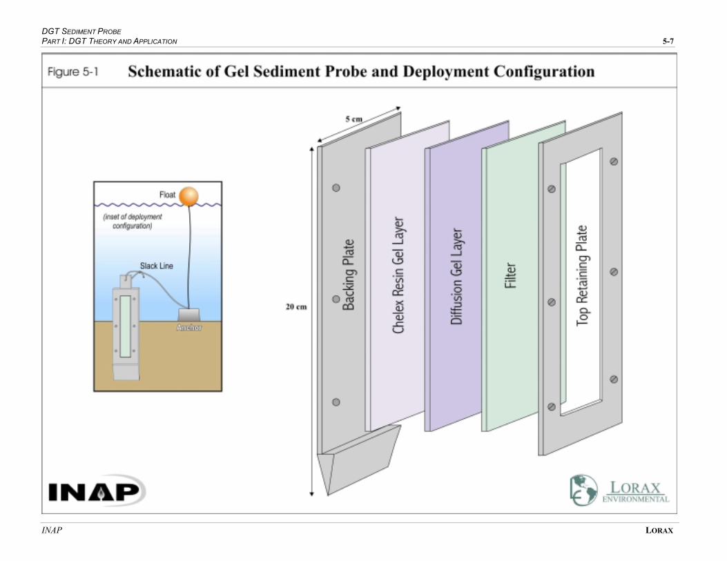
DGT SEDIMENT PROBE PART I: DGT THEORY AND APPLICATION 5-7
INAP LORAX

DGT SEDIMENT PROBE PART I: DGT THEORY AND APPLICATION 5-8
INAP LORAX
Provided that porewater metal concentrations at the porewater-diffusion-layer interface
remain the same during DGT deployment and knowing the diffusion characteristics of the
gel layer (i.e., thickness of diffusive layer and published molecular diffusion coefficients
in water), time of deployment and mass of metal on the resin, the concentration of metal
in the pore water may be calculated using Fick’s first law of diffusion (analogous to the
DGT water sampler described in Chapter 4). However, there are two complications in
this approach that are unique to the sediment probe, these are: 1) perturbation of pore
water concentrations; 2) lack of precise estimates of the diffusion coefficients for species
within the gel itself; and 3) vertical diffusion of metals within the diffusive (gel) layer.
These complicating factors are discussed below.
The introduction of the DGT probe perturbs the pore water system in a well-characterized
fashion (by introducing a local sink) while simultaneously recording a response. Metals
diffuse from pore waters to the DGT device where they are bound to the resin. The DGT
device therefore induces a flux from pore water, which may deplete the local pore water
concentration. The magnitude of this local depletion in pore water concentrations
depends on the re-supply rate of “exchangeable” metals to the pore water from the solid
phase (due to changes in equilibrium between pore water and solid phase). The processes
which remove exchangeable metals to the solid phase include adsorption, absorption and
surface precipitation, collectively referred to as “sorption”; metals are remobilized by
desorption, the reverse process. Based on the observed kinetics of metal remobilization
in DGT studies, re-supply of metals to pore waters is controlled by these
sorption/desorption processes (Harper et al., 1998).
Based on the relative flux of a given metal from pore waters to the DGT and the rate of
re-supply to pore waters from the solid phase, local pore water concentrations may be
affected in three possible ways (Zhang et al., 1998c). The cases where pore waters are
well buffered and the re-supply from the solid phase maintains constant pore water
concentrations, will be referred to in the subsequent discussion as the “sustained case”.
The “partially sustained case” refers to the situation where there is some re-supply, but is
insufficient to prevent some decrease in local pore water concentrations. The
“unsustained case” refers to the situation where there is no significant re-supply from the
solid phase and that local pore water concentrations decrease with time during DGT
deployment.
The sustained case occurs when there is both a fast rate of, and high capacity for, re-
supply to pore waters from the solid phase. Pore water concentrations are therefore not
depleted during DGT deployment. This is shown schematically in Figure 5-2 (a), where
pore water metal concentrations remain constant during DGT deployment.

DGT SEDIMENT PROBE PART I: DGT THEORY AND APPLICATION 5-9
INAP LORAX
DGT SEDIMENT PROBE PART I: DGT THEORY AND APPLICATION 5-10
INAP LORAX
Determination of pore water metal concentrations using DGT is based on Fick’s first law
of diffusion. Pore water concentrations (C) may be calculated, according to:
C = M∆g/(DtA)
Where, M is the mass of the metal accumulated in the resin layer, ∆g is the thickness of
the diffusive layer (Figure 5-2), D is the diffusion coefficient of a given metal ion and A
is the area of the gel membrane exposed to pore waters. Note that D is typically assumed
to be the same in the gel as it is in water. This is not necessarily true; D may well be less
in the gel than in pure water. Ideally, Dgel should be determined experimentally for each
species of interest.
The partially sustained case occurs when there is some re-supply from the solid phase,
but is insufficient to prevent depletion of local pore water concentrations. This is shown
schematically in Figure 5-2 (b), where pore water concentrations adjacent to the DGT
device decrease during deployment, and thus the rate of metal binding by the resin
decreases over time. In this case, the flux of metal from pore water to the DGT probe
represents a remobilization flux from solid phase to solution.In the unsustained case,
there is no re-supply of metal from the solid phase. This occurs because there is either no
exchangeable metal bound to the solid phase or that the rate of desorption from the solid
phase is slow, resulting in an insignificant re-supply rate to pore waters during the
deployment period. In this case, DGT data represent the diffusive flux from adjacent
pore waters to the DGT sediment probe.
Two different approaches have been adopted to differentiate between the three cases
outlined above. Firstly, DGT-derived pore water concentrations may be compared to
independent pore water determinations using conventional techniques (e.g., Zhang et al.,
1995a, b). The main disadvantage of this approach is the incompatible spatial resolution
of DGT (sub-millimeter scale) and conventional techniques (sub-centimeter scale).
Secondly, data from DGT devices of varying gel thickness have been used to distinguish
between the three possible cases (e.g., Hooda et al., 1999). By varying the thickness of
the diffusive layer, the flux to the resin is effectively altered (i.e., uptake by DGT
decreases with increasing thickness of the gel layer). Hooda et al. (1999) claimed that in
a graph of the measured mass of metal per unit area versus reciprocal of diffusive (gel)
layer thickness (M vs. 1/∆g), a linear plot represents the sustained case and a non-linear
relationship indicates that re-supply to pore waters from the solid phase is less than DGT
uptake. Of course, increasing the gel thickness will also increase the fraction of labile
metal measured by DGT, as noted earlier in this report (Section 4.3.1), and this needs to
be taken into account.
DGT SEDIMENT PROBE PART I: DGT THEORY AND APPLICATION 5-11
INAP LORAX
The second consideration unique to the DGT sediment probe is that vertical pore water
concentration profiles may become relaxed, particularly where large chemical gradients
foster vertical diffusion in the gel layer. The extent of this relaxation is dependent on gel
layer thickness and the chemical gradient in pore waters (Harper et al., 1999a; 1999b).
This artifact of the technique can be minimized by decreasing the gel thickness in high
chemical gradients (Davison et al., 1994).
5.3.2 DGT Sediment Probe Applications
The DGT sediment probe has great potential as a tool to improve assessment techniques
in two areas of interest to the mining industry: subaqueous sediment/tailings reactivity
and sediment toxicity studies. The DGT sediment probe has undergone extensive testing
and verification in order to minimize artifacts associated with use of the device. For
example, oxygenation artifacts in anoxic pore waters (e.g., FeOOH formation in the gel
due to the presence of molecular oxygen in the gel and in the lattice of the Perspex probe)
have been overcome by deoxygenating the DGT sediment probe prior to deployment
(Davison et al., 1994; Davison et al., 1997b). DGT sediment probes have also been used
in a number of studies to elucidate sediment and soil pore water chemistry and re-supply
rates from the solid phase. A summary of the published scientific literature is presented
in the following paragraphs.
Zhang et al. (1995a; 1995b) conducted in situ measurement of Fe, Mn, Cu, Ni, Cd and Zn
at sub-millimetre resolution in lacustrine pore waters. Zn and Cd in pore waters were
well buffered by rapid equilibria with the solid phase allowing measurement of their
concentrations. Mn was not released to pore waters and therefore supply to DGT was
solely by diffusion. Ni, Cu and Fe represented intermediate cases with a partial re-supply
from the solid phase and provided a direct measure of the mean in situ flux from solid to
solution phase for a 24 h deployment period.
Davison et al. (1997) made in situ measurements of Zn, Mn, Fe and As (III) by DGT in
stream sediments and microbial mats at 100-micron resolution. This study showed the
importance of the high spatial resolution achievable by DGT in determining fluxes of
metals across the sediment-water boundary, as remobilization typically occurs in the top
few millimeters of the sediments.
Harper et al. (1998a) used a two-dimensional numerical model (combining existing solid-
solution interaction model and a simple diffusion model) and DGT data to study sorption
rate constants. In cases where there is no rapid re-supply from the solid phase, DGT
provides a remobilization flux from solid to solution (areal flux). The authors developed
a method to express DGT data as a volumetric flux so that they can be related to the mass
DGT SEDIMENT PROBE PART I: DGT THEORY AND APPLICATION 5-12
INAP LORAX
of the solid phase. This enables the DGT flux to be expressed as a desorptive flux per
unit volume of sediment (i.e., mol/cm3/s).
Zhang, et al. (1998c) and Hooda et al. (1999) conducted laboratory studies to determine
labile metal concentrations in soil solutions and the bioavailability of metals (Cd, Co, Cu,
Ni, Pb and Zn) bound to the solid phase using DGT, while Harper et al. (1999a) and
Shuttleworth et al. (1999) studied the effects of horizontal heterogeneity and microniches
on interpretation of pore water data and process rate (flux) determinations.
5.4 Summary
The DGT sediment probe is a potentially powerful tool for investigations of subaqueous
sediment/tailings reactivity and sediment toxicity. The flux of metal from pore water to
the DGT probe may be used either to calculate in some cases a concentration of the labile
fraction in pore waters or to quantify a remobilization flux from solid to solution.
The main advantage of DGT over conventional pore water sampling techniques is the
high spatial resolution (sub-millimetre resolution) and minimal sampling artifacts. In
respect to toxicity assessments, DGT provides both in situ labile (bioavailable) metal
concentrations and the remobilization flux from the solid phase. This information may be
used to determine the bioavailable metal inventory both in pore waters and the solid
phase. The main advantage of DGT over existing toxicity techniques (e.g., pore water
extractions, sequential extractions and solid phase chemistry) is that the metal inventory
potentially available to benthic organisms may be estimated under realistic field
conditions. In addition, DGT deployment procedures are relatively simple and
inexpensive compared to other techniques.
Although extensive work has been conducted on the internal QA/QC for the DGT
sediment probe, additional work is required prior to its routine application to
environmental issues faced by the mining industry. The main areas in which further
research are required are:
• speciation studies in pore waters to determine more precisely the nature of metal
species measured by DGT; and
• correlation with conventional toxicity techniques to determine the utility of the
DGT probe as an in situ toxicity indicator given a spectrum of different types and
behaviours of benthic organisms.
Since comprehensive toxicological assessments are presently conducted by integration of
several methods, the DGT sediment probe may become an important tool once additional
speciation and toxicity work has been conducted. For example, integration of data from

DGT SEDIMENT PROBE PART I: DGT THEORY AND APPLICATION 5-13
INAP LORAX
DGT and other techniques (e.g., bioassays, community structure assessments, etc.) may
result in significant improvements in both toxicity assessments and in understanding the
mechanisms of metal bioavailability.

International Network for Acid Preventi
References
R-1
References
Absil, M. C. P., J. J. Kroon, et al. (1994). “Availability of copper from phytoplankton and water for the bivalve Macoma balthica. II. Uptake and elimination from 64Cu-labelled diatom and water.” Mar. Biol. 118: 129-135.
Achterberg, E. P. and C. Braungardt (1999). “Stripping voltammetry for the determination of trace metal speciation and in situ measurements of trace metal distributions in marine waters.” Anal. Chim. Acta 400: 381-397.
Achterberg, E. P. and C. M. G. Vandenberg (1994). “Automated Voltammetric System for Shipboard Determination of Metal Speciation in Sea-Water.” Anal. Chim. Acta 284: 463-471.
Ahner, B. A. and F. M. M. Morel (1995). “Phytochelatin production in marine algae. 2. Induction by various metals.” Limnol. Oceanogr. 40: 658-665.
Ahner, B. A., F. M. M. Morel, et al. (1997). “Trace metal control of phytochelatin production in coastal waters.” Limnol. Oceanogr 42(3): 601-608.
Alberic, P., E. Viollier, et al. (2000). “Interactions between trace elements and dissolved organic matter in the stagnant anoxic deep layer of a meromictic lake.” Limnol. Oceanogr 45(5): 1088-1096.
Alfaro-De la Torre, M. C., P. Y. Beaulieu, et al. (2000). “In situ measurement of trace metals in lakewater using the dialysis and DGT techniques.” Anal. Chim. Acta 418(1): 53-68.
Allison, J.D., Brown, D.S. and Novo-Gradac, K.J. (1991). "MINTEQA2/PRODEFA2, a geochemical assessment model for environmental systems: version 3.0 user’s manual". U.S. Environmental Protection Agency, Athens, Ga.
Anderson, D. M. and F. M. M. Morel (1979). “Copper sensitivity of Gonyaulax tamarensis.” Limnol . Oceanogr. 23: 283-295.
Anderson, S. L., F. M. M. Morel, et al. (1978). “Growth limitation of a coastal diatom by low zinc ion activity.” Nature 276: 70-72.
Ankley, G.T., Thomas, N.A., Di Toro, D.M., Hansen, D.J., Mahony, J.D., Berry, W.J., Swartz, R.C., Hoke, R.A., Garrison, A.W., Allen, H.E., and Zarba, C.S. (1994). "Assessing potential bioavailability of metals in sediments: a proposed approach." Environ. Man.. 18: 331-337.
Baillieul, M. and R. Blust (1999). “Analysis of the swimming velocity of cadmium-stressed Daphnia magna.” Aquat. Toxicol. 44(4): 245-254.
Barata, C., D. J. Baird, et al. (1998). “Influence of genetic and environmental factors on the tolerance of Daphnia magna Straus to essential and non-essential metals.” Aquatic Toxicology 42(2): 115-137.
Beauchemin, D., McLaren, J. W., Mykytiuk, A. P. and Berman, S. S. (1987). “Determination of trace metals in a river water reference material by inductively coupled plasma mass spectrometry.” Anal. Chem. 59: 778 - 783.
REFERENCES PART I: DGT THEORY AND APPLICATION R-2
INAP LORAX
Bedsworth, W. W. and D. L. Sedlak (1999). “Sources and Environmental Fate of Strongly Complexed Nickel in Estuarine Waters: The Role of Ethylenediaminetetraacetate.” Environ. Sci. Technol 33: 926-931.
Bervoets, L. and R. Blust (1999). “Bioavailability of cadmium and zinc to midge larvae under natural and experimental conditions: Effects of some environmental factors.” Belg. J. Zool. 129(1): 269-284.
Bervoets, L. and R. Blust (2000). “Effects of pH on cadmium and zinc uptake by the midge larvae Chironomus riparius.” Aquat. Toxicol. 49(1-2): 145-157.
Boyle, E. A., F. Sclater, et al. (1976). “On the marine geochemistry of cadmium.” Nature 263(5572): 42-44.
Bruland K. W. (1992). Complexation of cadmium by natural organic ligands in the central North Pacific. Limnol. Oceanogr. 37: 1008-1017.
Bruland K. W., Franks R. P., Knauer G. A., and Martin J. H. (1979). Sampling and analytical methods for the determination of copper, cadmium, zinc and nickel at the nanogram per liter level in sea water. Anal. Chim. Acta 105: 233-245.
Bruland, K. W. (1989). “Complexation of zinc by natural organic ligands in the central North Pacific.” Limnol. Oceanogr. 34: 269-285.
Buffle, J., K. J. Wilkinson, et al. (1997). “In situ monitoring and speciation of trace metals in natural waters.” Annali di Chimica 87: 67-82.
Burton, G.A. (1992). "Sediment collection and processing: factors affecting realism". In Sediment Toxicity Assessment. Ed: G.A. Burton. Lewis Publishers, Chelsea, Mich. pp. 37-66.
Campbell P. G. C. (1995). "Interactions between trace metals and aquatic organisms: a critique of the free-ion activity model." In Metal Speciation and Bioavailability in Aquatic Systems (ed. A. Tessier and D. R. Turner). John Wiley and Sons. pp. 45-102.
Carter, R. J., A. Hoxey, et al. (1992). “Complexation capacity of sediment humic acids as a function of extraction technique.” Sci. Tot. Env. 125: 25-31.
Carvalho, R. A., M. C. Benfield, et al. (1999). “Comparative bioaccumulation studies of colloidally-complexed and free-ionic heavy metals in juvenile brown shrimp Penaeus aztecus (Crustacea : Decapoda : Penaeidae).” Limnol. Oceanogr. 44(2): 403-414.
Chakrabarti, C. L., Y. J. Lu, et al. (1994). “Kinetic-studies of metal speciation using Chelex cation-exchange resin - application to cadmium, copper, and lead speciation in river water and snow.” Environ. Sci. Technol. 28(11): 1957-1967.
Chang, J. C., P. B. Taylor, et al. (1981). “Use of the Microtox assay system for environmental samples.” Bull. Environ. Contam. Toxicol. 26(2): 150-156.
Chang, L., W. Davison, et al. (1998). “Performance characteristics for the measurement of Cs and Sr by diffusive gradients in thin films (DGT).” Anal. Chim. Acta. 368(3): 243-253.
Chapman, P. M., F. Y. Wang, et al. (1998). “Ecotoxicology of metals in aquatic sediments: binding and release, bioavailability, risk assessment, and remediation.” Can. J. Fish. Aquat. Sci. 55(10): 2221-2243.
REFERENCES PART I: DGT THEORY AND APPLICATION R-3
INAP LORAX
Cheng, J. G., C. L. Chakrabarti, et al. (1994). “Chemical speciation of Cu, Zn, Pb and Cd in rain water.” Anal. Chim. Acta 288(3): 141-156.
Chramback, A. (1985) "The Principles of Quantitative Gel Electrophoresis". Weinheim, Germany.
Coale, K. H. and K. W. Bruland (1988). “Copper complexation in the northeast Pacific.” Limnol. Oceanogr. 33: 1084-1101.
Codina, J. C., A. Perez-Garcia, et al. (1993). “A comparison of microbial bioassays for the detection of metal toxicity.” Arch. Environ. Contam. Toxicol. 25(2): 250-254.
Cotton, F. A. and G. Wilkinson (1980). Advanced Inorganic Chemistry, John Wiley & Sons.
Craig, A., L. Hare, et al. (1999). “Experimental evidence for cadmium uptake via calcium channels in the aquatic insect Chironomus staegeri.” Aquat. Toxicol. 44(4): 255-262.
Croot, P. L., J. W. Moffett, et al. (2000). “Production of extracellular Cu complexing ligands by eukaryotic phytoplankton in response to Cu stress.” Limnol. Oceanogr. 45(3): 619-627.
Davis, J. A. and J. O. Leckie (1978). “Effect of adsorbed complexing ligands on trace metal uptake by hydrous oxides.” Environ. Sci. Technol. 12(12): 1309-1315.
Davison, W., G. W. Grime, et al. (1991). “Distribution of dissolved iron in sediment pore waters at submillimetre resolution.” Nature 352: 323-324.
Davison, W. and H. Zhang (1994.). “In situ speciation measurements of trace components in natural waters using thin-film gels.” Nature 367: 546-548.
Davison, W. and H. Zhang (2000). "In situ measurements of labile species in waters and sediments using DGT". In Chemical Sensors in Oceanography. M. Varney (Ed.), Gordon and Breach.
Davison, W. Fones, G., Harper, M., Teasdale, P and Zhang, H. (2000) "Dialysis, DET and DGT: in situ diffusional techniques for studying water, sediments and soils". In: In situ Chemical Analyses in Aquatic Systems. Eds. J. Buffle and G. Horvai. Wiley.
Davison, W., G. R. Fones, et al. (1997a). “Dissolved metals in surface sediment and a microbial mat at 100 um resolution.” Nature 387: 885-888.
Davison, W., H. Zhang, et al. (1997b). "In situ procedures for measuring chemical speciation and availability of trace metals in soils and sediments". In: Contaminated Soils. R. Prost. Paris, INRA.
Davison, W., H. Zhang, et al. (1994). “Developing and applying new techniques for measuring steep chemical gradients of trace metals and inorganic ions at the sediment-water interface.” Mineral. Mag. 58a: 215-216.
Denney, S., J. Sherwood, et al. (1999). “In situ measurements of labile Cu, Cd, and Mn in river waters using DGT.” Sci. Tot. Environ. 239(1-3): 71-80.
Donat, J. R., K. A. Lao, et al. (1994). “Speciation of dissolved copper and nickel in South San- Francisco Bay - a multimethod approach.” Anal. Chim. Acta 284(3): 547-571.
REFERENCES PART I: DGT THEORY AND APPLICATION R-4
INAP LORAX
dosSantos, M. M. C., M. L. S. Goncalves, et al. (1996). “Cadmium and lead complexation by anodic stripping voltammetry with a mercury microelectrode.” Electroanalysis 8(2): 178-182.
Dunn, M. J. (1993). Gel Electrophoresis: Proteins. Bios Scientific. Oxford, UK.
Ellis, D.V. and MacDonald, V.I. (1998). "Rapid preliminary assessment of seabed biodiversity for the marine and coastal mining industry". Mar. Geores. Geotech. 16: 307-319.
Engel, D.W., W. Sunda and B.A. Fowler (1981). "Factors affecting trace metal uptake and toxicity to estuarine organisms. I. Environmental parameters. In: Biological Monitoring of Marine Pollutants, F. J. Vernberg et al. (Eds.). Academic Press, New York.
Errecalde, O. and P. G. C. Campbell (2000). “Cadmium and zinc bioavailability to Selenastrum capricornutum (Chlorophyceae): accidental metal uptake and toxicity in the presence of citrate.” J. Phycol. 3: 473-483.
Errecalde, O., M. Seidl, et al. (1998). “Influence of a low molecular weight metabolite (citrate) on the toxicity of cadmium and zinc to the unicellular green alga Selenastrum capricornutum: An exception to the free-ion model.” Wat. Res. 32(2): 419-429.
Fisher, N. S. (1986). “On the reactivity of metals for marine phytoplankton.” Limnol. Oceanogr. 31: 443-449.
Florence, T. M. (1982). “The speciation of trace elements in waters.” Talanta 29: 345-364.
Franklin, N. M., J. L. Stauber, et al. (2000). “pH-dependent toxicity of copper and uranium to a tropical freshwater alga (Chlorella sp.).” Aquat. Toxicol. 48(2-3): 275-289.
Gagnon, C. and N. S. Fisher (1997). “Bioavailability of sediment-bound methyl and inorganic mercury to a marine bivalve.” Environ. Sci. Tech. 31(4): 993-998.
Gledhill, M., M. Nimmo, et al. (1999). “The release of copper-complexing ligands by the brown alga Fucus vesiculosus (Phaeophyceae) in response to increasing total copper levels.” J. Phycol. 35(3): 501-509.
Gundersen, J. K. and B. B. Jorgensen (1990). “Microstructure of diffusive boundary layers and the oxygen uptake of the sea floor.” Nature 345: 604-607.
Gutknecht, J. (1981). “Inorganic mercury (Hg2+) transport through lipid bilayer membranes.” J. Membrane Biol. 61: 61-66.
Hao, O. J., C.-J. Shin, et al. (1996). “Use of Microtox test for screening industrial wastewater toxicity.” Wat. Sci. Technol. 34(10): 43-50.
Hare, L. and A. Tessier (1996). “Predicting animal cadmium concentrations in lakes.” Nature 380: 430-432.
Hare, L., A. Tessier and L. Warren (2001). “Cadmium accumulation by invertebrates living at the sediment-water interface”. Environ. Toxicol. Chem. 20, 880-889.
Harper, M. P., W. Davison, et al. (1998). “Kinetics of metal exchange between solids and solutions in sediments and soils interpreted from DGT measured fluxes.” Geochim. Cosmochim. Acta. 62(16): 2757-2770.
REFERENCES PART I: DGT THEORY AND APPLICATION R-5
INAP LORAX
Harper, M. P., W. Davison, et al. (1999a). “Estimation of pore water concentrations form DGT and DET techniques.” Anal. Chem. Acta. 398.: 329-340.
Harper, M., W. Davison, et al. (1999b). “Estimation of pore water concentrations from DGT profiles: a modelling approach.” Aquat. Geochem. 5: 337-355.
Herbelin, A.L. and Westall, J.C. (1996). "FITEQL – a computer program for determination of chemical equilibrium constants from experimental data". Rep. 96-01, Department of Chemistry, Oregon State University, Corvallis, Oreg.
Hill, S. J. (1997). “Speciation of trace metals in the environment.” Chem. Soc. Rev. 26(4): 291-298.
Hirose K. and Sigimura Y. (1985). "Role of metal-organic complexes in the marine environment - A comparison of the copper and ligand titration methods". Mar. Chem. 16: 239-247.
Hodson, P. V., B. R. Blunt, et al. (1978). “pH-induced changes in blood lead of lead-exposed rainbow trout (Salmo gairdneri).” J. Fish. Res. Board Can. 35: 437-445.
Hollis, L., K. Burnison, et al. (1996). “Does the age of metal-dissolved organic carbon complexes influence binding of metals to fish gills?.” Aquat. Toxicol. 35: 253-264.
Hooda, P. S., H. Zhang, et al. (1999). “Measuring bioavailable trace metals by diffusive gradients in thin films (DGT): soil moisture effects on its performance in soils.” Euro. J. Soil Sci. 50: 1-10.
Hudson, R. J. M. (1998). “Which aqueous species control the rates of trace metal uptake by aquatic biota? Observations and predictions of non- equilibrium effects.” Sci. Tot. Env. 219(2-3): 95-115.
Ingersoll, C.G., Ankley, G.T., Benoit, D.A., Brunson, E.L., Burton, G.A., Dwyer, F.J., Hoke, R.A., Landrum, P.F., Norberg-King, T.J. and Winger, P.V. (1995). "Toxicity and bioaccumulation of sediment-associated contaminates using freshwater invertebrates: a review of methods and applications". Environ. Toxicol. Chem., 14: 1885-1894.
Jackson, T. A. and T. Bistricki (1995). “Selective scavenging of Cu, Zn, Pb, and As by Fe and Mn oxyhydroxide coatings in lakes polluted with mine and smelter wastes: results of energy dispersive X-ray micro-analysis.” J. Geochem. Explor. 52: 97-125.
Jansen, R. A. G., H. P. Van Leeuwen, et al. (1998). “Speciation and lability of zinc(II) in river waters.” Environ. Sci. Tech. 32(24): 3882-3886.
Karbassi, A. R. and S. Nadjafpour (1996). “Flocculation of dissolved Pb, Cu, Zn and Mn during estuarine mixing of river water with the Caspian Sea.” Env. Poll. 93(3): 257-260.
Keller, O. C. and J. Buffle (2000). “Voltammetric and reference microelectrodes with integrated microchannels for flow through microvoltammetry. 2. Coupling the microcell to a supported liquid membrane preconcentration technique.” Anal. Chem. 72(5): 943-948.
Keller, O. C., S. Poitry, et al. (1994). “A hollow-fiber supported liquid membrane system for metal speciation and preconcentration - Calculation of the response-time.” J. Electroanal. Chem. 378(1-2): 165-175.
Koretsky, C. (2000). “The significance of surface complexation reactions in hydrologic systems: a geochemist's perspective.” J. Hydrol. 230(3-4): 127-171.

REFERENCES PART I: DGT THEORY AND APPLICATION R-6
INAP LORAX
Kozelka, P. B. and K. W. Bruland (1998). “Chemical speciation of dissolved Cu, Zn, Cd, Pb in Narragansett Bay, Rhode Island.” Mar. Chem. 60: 267-282.
Krom M.D., Davison P., Zhang H., and Davison W. (1994) "High-resolution pore water sampling with a gel sampler". Limnol. Oceanogr. 39(8), 1967-1972.
Krom, M.D., Davison, P., Zhang, H and Davison, W. (1995). "High resolution pore water sampling using a gel sampler: an innovative technique". Limnol. Oceanogr., 39: 1967-1972.
Laporte, J. M., J. P. Truchot, et al. (1997). “Combined effects of water pH and salinity on the bioaccumulation of inorganic mercury and methylmercury in the shore grab Carcinus maenas.” Mar. Poll. Bull. 34(11): 880-893.
Laxen, D. P. H. (1985). “Trace metal adsorption / coprecipitation on hydrous ferric oxide under realistic conditions.” Wat. Res. 19(10): 1229-1236.
Leal, M. F. C., M. T. S. D. Vasconcelos, et al. (1999). “Copper-induced release of complexing ligands similar to thiols by Emiliania huxleyi in seawater cultures Limnol. Oceanogr 44: 1750-1762.
Lee, J. G., B. Ahner, et al. (1996). “Export of cadmium and phytochelatin by the marine diatom Thalassiosira weissfloglii.” Environ. Sci. Tech. 30: 1814-1821.
Legras, S., C. Mouneyrac, et al. (2000). “Changes in metallothionein concentrations in response to variation in natural factors (salinity, sex, weight) and metal contamination in crabs from a metal-rich estuary.” J. Exp. Mar. Biol. Ecol. 246(2): 259-279.
Li, Y. H. and S. Gregory (1974). “Diffusion of ions in sea water and in deep-sea sediments.” Geochmim. Cosmochim. Acta. 38: 703-714.
Lorax, (1999). "Subaqueous Reactivity of Marcopper Tailings". Prepared for Placer Dome Asia
Pacific. Prepared by Lorax Environmental Services Ltd.
Luoma, S. N., R. Dagovitz, et al. (1990). “Temporally intensive study of trace metals in sediments and bivalves from a large river-estuarine system: Suisun Bay/delta in San Francisco Bay.” Sci. Tot. Env. 97/98: 685-712.
Manheim, F. T. (1970). “The diffusion of ions in unconsolidated sediments.” Earth Planet. Sci. Lett. 9: 307-309.
Martin, A. J., J. J. McNee and Pedersen, T.F.. (2001). “The reactivity of sediments impacted by metal-mining in Lago Junin, Peru.” J. Geochem. Explor.: 175-187
Mayer, L. M., Z. Chen, et al. (1996). “Bioavailability of sedimentary contaminants subject to deposit-feeder digestion.” Environ.Sci. Technol. 30: 2641-2645.
McGeer, J. C. and C. M. Wood (1998). “Protective effects of water Cl on physiological responses to waterborne silver in rainbow trout.” Can. J. Fish. Aquat. Sci. 55(11): 2447-2454.
McNee, J. J. and Martin, A. J (1999). "The measurement of biologically-available metals in aquatic systems and mine effluents – a new approach" Presented at “Tailings and Mine Waste, 99”, Fort Collins, CO.
REFERENCES PART I: DGT THEORY AND APPLICATION R-7
INAP LORAX
McNee, J. J. and Robertson, J. D (1998) "Development of a new sampling device to measure biologically-available metals in natural waters and mine effluents". CIM Journal: CIM Paper No. 8135.
MEND (1995). "GEOCHEMICAL ASSESSMENT OF SUBAQUEOUS TAILINGS DISPOSAL IN BUTTLE
LAKE, B.C., 1993 STUDY PROGRAM", MEND REPORT 2.11.4A.
Meyer, J. S. (1999). “A mechanistic explanation for the In(LC50) vs. In(hardness) adjustment equation for metals.” Env. Sci. Tech. 33(6): 908-912.
Meyer, J. S., R. C. Santore, et al. (1999). “Binding of nickel and copper to fish bills predicts toxicity when water hardness varies, but free-ion activity does not.” Env. Sci. Tech. 33(6): 913-916.
Miller, W. E., S. A. Peterson, et al. (1985). “Comparative toxicology of laboratory organisms for assessing hazardous waste sites.” J. Environ. Qual. 14: 29-32.
Moffett, J. W. and L. E. Brand (1996). “The production of strong Cu chelators by marine cyanobacteria in response to Cu stress.” Limnol Oceanogr. 41: 388-395.
Muller, F. L. L. and D. R. Kester (1991). “Measurement of the different forms of zinc in Narragansett Bay water based on the rate of uptake by a chelating resin.” Mar. Chem. 33: 171-186.
Nirel, P.M.V. and Morel, F.M.M. (1990). "Pitfalls of sequential extractions". Wat. Res. 24: 1055-1056.
Nordstrom, D. K. (1996). “Trace Metal Speciation in Natural Waters: Computational vs. Analytical.” Wat. Air Soil Poll. 90: 257-267.
Nriagu J. O., Lawson G., Wong H. K. T., and Azcue J. M. (1993). "A protocol for minimizing contamination in the analysis of trace metals in Great Lakes waters". J. Great Lakes Res. 19(1), 175-182.
Nriagu, J. O., H. K. T. Wong, et al. (1981). “Particulate and dissolved trace metals in Lake Ontario.” Wat. Res. 15: 91-96.
Nriagu, J. O., H. K. T. Wong, et al. (1982). “Deposition and chemistry of pollutant metals in lakes around the smelters at Sudbury, Ontario.” Environ. Sci. Technol. 16: 551-560.
O'Day, P. A., S. A. Carroll, et al. (2000). “Metal speciation and bioavailability in contaminated estuary sediments, Alameda Naval Air Station, California.” Environ. Sci. Tech 34(17): 3665-3673.
Pai S. C., Fang T. H., Chen C. T. A., and Jeng K. L. (1990). "A low contamination Chelex-100 technique for shipboard pre-concentration of heavy metals in seawater". Mar. Chem. 29: 295-306.
Pardo, R., E. Barrado, et al. (1994). “Voltammetric complexation capacity of waters of the Pisuerga River.” Wat. Res. 28: 2139-2146.
Parkhurst, D. L., D. C. Thorstenson, et al. (1980). "PHREEQE--A computer program for geochemical calculations": U.S. Geological Survey Water Resources Investigations Report.
REFERENCES PART I: DGT THEORY AND APPLICATION R-8
INAP LORAX
Parthasarathy, N. and J. Buffle (1994). “Capabilities of Supported Liquid Membranes for Metal Speciation in Natural-Waters - Application to Copper Speciation.” Anal. Chim. Acta 284(3): 649-659.
Paulson A. J. (1986) "Effects of flow rate and pretreatment on the extraction of trace metals from estuarine and coastal seawater by Chelex-100." Anal. Chem. 58: 183 - 187.
Pedersen, S.N., Lundebye, A.K. and Depledge, M.H. (1997). "Field application and metallothionein and stress protein biomarkers in the shore crab (Carcinus maenas) exposed to trace metals". Aquat. Toxicol. 37: 183-200.
Pedersen, T.F., McNee, J.J., Flather, D.H., Mueller, B., Sahami, A.R., Pelletier, C.A. (1997). "Geochemistry of submerged tailings in Buttle Lake and the Equity Silver tailings pond, British Columbia, and Andersen Lake, Manitoba: what have we learned?" Proceedings, Fourth International Conference on Acid Rock Drainage. Vancouver, June 1997.
Petronio, B. M., B. Cosma, et al. (1993). “A Multimethod Approach to Study Humic Compounds and Metal Speciation in Marine Sediment Samples.” International Journal of Environmental Analytical Chemistry 54(1): 45-56.
Phinney, J. T. and K. W. Bruland (1997). “Effects of dithiocarbamate and 8-hydroxyquinoline additions on algal uptake of ambient copper and nickel in South San Francisco Bay water.” Estuaries 20(1): 66-76.
Playle, R. C. (1998). “Modelling metal interactions at fish gills.” Sci. of the Tot. Env. 219(2-3): 147-163.
Prygiel, J., A. Rosso-Darmet, et al. (1999). “Use of oligochaete communities for assessment of ecotoxicological risk in fine sediment of rivers and canals of the Artois-Picardie water basin (France).” Hydrobiologia 410: 25-37.
Rainbow, P. S., C. Amiard-Triquet, et al. (2000). “Observations on the interaction of zinc and cadmium uptake rates in crustaceans (amphipods and crabs) from coastal sites in UK and France differentially enriched with trace metals.” Aquat. Toxicol. 50(3): 189-204.
Reinfelder, J. R., N. S. Fisher, et al. (1998). “Trace element trophic transfer in aquatic organisms: A critique of the kinetic model approach.” Sci. Tot. Env. 219(2-3): 117-135.
Reinfelder, J. R., R. E. Jablonka, et al. (2000). “Metabolic responses to subacute toxicity of trace metals in a marine microalga (Thalassiosira weissflogii) measured by calorespirometry.” Environ. Toxicol. Chem. 19(2): 448-453.
Revsbech N.P. and Jørgensen B.B. (1986) "Microelectrodes: their use in microbial ecology". In: Advances in Microbial Ecology (K.C. Marshall, ed.) pp. 293-352.
Roditi, H. A., N. S. Fisher, et al. (2000). “Uptake of dissolved organic carbon and trace elements by zebra mussels.” Nature 407(6800): 78-80.
Roesijadi, G. (1992). “Metallothioneins in metal regulation and toxicity in aquatic animals.” Aquat. Toxicol. 22: 81-114.
Roesijadi, G. and B. Fowler (1992). "Purification of invertebrate metallothioneins" In: Metallobiochemistry, Part B: Metallothionein and related molecules. J. F. Riordan and B. L. Vallee. San Diego, Academic Press.

REFERENCES PART I: DGT THEORY AND APPLICATION R-9
INAP LORAX
Ross, A. R. S., M. G. Ikonomou, et al. (2000). “Characterization of dissolved tannins and their metal-ion complexes by electrospray ionization mass spectrometry.” Anal. Chim. Acta 411(1-2): 91-102.
Roy, R. and P. G. C. Campbell (1995). “Survival-Time Modeling of Exposure of juvenile Atlantic Salmon (Salmo-Salar) to Mixtures of Aluminum and Zinc in Soft-Water at Low Ph.” Aquat. Toxicol. 33(2): 155-176.
Sahami, A.R., and Riehm, D (1999). "An assessment of the subaqueous reactivity of sulphide-rich mine tailings from the Petaquilla Property, Panama". The Canadian Mining and Metallurgical (CIM) Bulletin. 92(1035): 77-80.
Santschi, P. H., P. Bower, et al. (1983). “ Estimates of the resistance to chemical transport posed by the deep-sea boundary layer.” Limnol. Oceanogr. 28: 899-912.
Sauve, S., M. B. McBride, et al. (1997). “Speciation of lead in contaminated soils.” Environ. Poll. 98(2): 149-155.
Savvides, C., A. Papadopoulos, et al. (1995). “Sea sediments contaminated with heavy metals: Metal speciation and removal.” Water Science and Technology 32(9-10): 65-73.
Sawamoto, H. (1999). “Adsorptive stripping voltammetry of metal ions (Review).” Bunseki Kagaku 48(2): 137-150.
Schecher, W.D. and McAvoy, W. (1994). "MINEQL+, user’s manual". Environmental Research
Software, Hallowell, Me.
Schramel, O., B. Michalke, et al. (1998). “Analysis of metal species by using electrospray ionization mass spectrometry and capillary electrophoresis electrospray ionization mass spectrometry.” J. Chromatography 819(1-2): 231-242.
Sedlak, D. L., J. T. Phinney, et al. (1998). “Strongly complexed Cu and Ni in wastewater effluents and surface runoff.” Environ. Sci.Technol. 31(10): 3010-3016.
Sholkovitz, E. R. (1976). “Flocculation of dissolved organic and inorganic matter during the mixing of river water and seawater.” Geochim. Cosmochim. Acta 40: 831-845.
Shuttleworth, S. M., W. Davison, et al. (1999). “Two-dimensional and fine structure in the concentrations of iron and manganese in sediment pore-waters.” Environ. Sci. Technol. 33: 4169-4175.
Sigg, L. (1985). "Metal transfer mechanisms in lakes; the role of settling particles". In: Chemical Processes in Lakes. W. Stumm, Wiley-Interscience.: 283-310.
Snell, T. W. and G. Persoone (1989). “Acute toxicity bioassays using rotifers: II. A freshwater test with Branchionus rubens.” Aqat. Toxicol. 14: 81-92.
Soegianto, A., M. Charmantier-Daures, et al. (1999). “Impact of cadmium on the structure of gills and epipodites of the shrimp Penaeus japonicus (Crustacea : Decapoda).” Aquatic Living Resources 12(1): 57-70.
Spry, D. J. and J. G. Weiner (1991). “Metal bioavailability and toxicity to fish in low-alkalinity lakes: a critical review.” Env. Pollution 71: 243-304.
Stumm, W. and J. J. Morgan (1981). Aquatic Chemistry. New York, Wiley-Interscience.
REFERENCES PART I: DGT THEORY AND APPLICATION R-10
INAP LORAX
Sturgeon, R. E., Berman, S. S., and Willie, S. N. (1982). “Concentration of trace metals from sea water by complexation with 8-hydroxyquinoline and adsorption on C18-bonded silica gel.” Talanta 29: 167-171.
Sunda, W. G. (1991). “Trace metal interactions with marine phytoplankton.” Biol. Oceanogr. 6: 411-417.
Sunda, W. G. and P. A. Gillespie (1979). “The response of a marine bacterium to cupric ion and its use to estimate cupric ion activity in seawater.” J. Mar. Res. 37: 761-772.
Sunda, W. G. and R. R. L. Guillard (1976). “The relationship between cupric ion activity and the toxicity of copper to phytoplankton.” J. Mar. Res. 34: 511-529.
Sunda, W. G. and S. A. Huntsman (1992). “Feedback interactions between zinc and phytoplankton in seawater.” Limnol. Oceanogr. 37: 25-40.
Sunda, W. G. and S. A. Huntsman (1998). “Processes regulating cellular metal accumulation and physiological effects: phytoplankton as model systems.” Sci. Tot. Env. 219: 183-208.
Sunda, W. G., P. A. Tesier, et al. (1987). “Effects of cupric and zinc ion activities on the survival and reproduction of marine copepods.” Mar. Biol. 94: 203-210.
Sunda, W.G. (1984). "Measurement of manganese, zinc and cadmium complexation in seawater using chelex ion exchange equilibria". Mar. Chem., 14: 365-378.
Taillefert, M., C.-P. Lienemann, et al. (2000). “Speciation, reactivity and cycling of Fe and Pb in a meromictic lake.” Geochim. Cosmochim. Acta 64: 169-183.
Teasdale, P. R., S. Hayward, et al. (1999.). “In situ, high-resolution measurement of dissolved sulfide using diffusive gradients in thin films with computer-imaging densitometry.” Analytical Chemistry. 71(11): 2186-2191.
Temminghoff, E. J. M., A. C. C. Plette, et al. (2000). “Determination of the chemical speciation of trace metals in aqueous systems by the Wageningen Donnan Membrane Technique.” Anal. Chim. Acta. 417(2): 149-157.
Tercier, M. L., J. Buffle, et al. (1998a). “Novel voltammetric in-situ profiling system for continuous real-time monitoring of trace elements in natural waters.” Electroanalysis 10(6): 355-363.
Tercier-Waeber, M. L., C. Belmont-Hebert, et al. (1998b). “Real-time continuous Mn(II) monitoring in lakes using a novel voltammetric in situ profiling system.” Environ. Sci. Technol. 32(10): 1515-1521.
Tercier-Waeber, M. L., J. Buffle, et al. (1999). “Submersible voltammetric probes for in situ real-time trace element measurements in surface water, groundwater and sediment-water interface.” Measurement Science & Technology 10(12): 1202-1213.
Tercier-Waeber, M. L., J. Buffle, et al. (2000). “Carrier-mediated transport of toxic elements through liquid membranes - Transport of Cd(II) from high salinity chloride medium through supported liquid membrane containing TBP/cyclohexane.” J. Membrane Sci. 177(1-2): 41-47.
Tessier, A., D. Fortin, et al. (1996). “Metal sorption to diagenetic iron and manganese oxyhydroxides and associated organic matter: narrowing the gap between field and laboratory measurements.” Geochem. Cosmochim. Acta 60(3): 387-404.

REFERENCES PART I: DGT THEORY AND APPLICATION R-11
INAP LORAX
Tessier, A., F. Rapin, et al. (1985). “Trace metals in oxic lake sediments: possible adsorption onto iron oxyhydroxides.” Geochem. Cosmochim. Acta 49: 183-194.
Tessier, A., P. G. C. Campbell, et al. (1979). “Sequential Extraction procedure for the speciation of particulate trace metals.” Anal. Chem. 51(7): 844-851.
Tessier, A., R. Carignan, et al. (1989). “Partitioning of Zn between the water column and the oxic sediments in lakes.” Geochim. Cosmochim. Acta. 53: 1511-1522.
Tessier, A., Y. Couillard, et al. (1993). “Modelling Cd partitioning in oxic lake sediments and Cd concentrations in the freshwater bivalve Anodonta grandis.” Limnol. Oceanogr. 38: 1-17.
Tipping, E. (1995). "WHAM – a chemical equilibrium model and computer code for waters, sediments, and soils incorporating a discrete site/electrostatic model of ion-binding by humic substances". Comp. Geosci., 20: 973-1023.
Tipping, E., S. Lofts, et al. (1998). “Modelling the chemical speciation of trace metals in the surface waters of the Humber system.” Sci. Tot. Environ. 210(1-6): 63-77.
Toussaint, M. W., T. R. Shedd, et al. (1995.). “A comparison of standard acute toxicity tests with rapid-screening toxicity tests.” Environ. Toxicol. Chem. 14(5): 907-915.
Van der Berg, G.A. (1998). "Determination of metal speciation in seawater using cathodic stripping voltammetry". In Metals in Surface Waters. Eds: H.E. Allen, W. Garrison, and G.W. Luther. Ann Arbor Press, Chelsea, Mich. Pp. 133-153.
Vega, M., R. Pardo, et al. (1995). “Pseudopolarographic Determination of Stability-Constants of Labile Zinc-Complexes in Fresh-Water.” Anal. Chim. Acta 310(1): 131-138.
Vela, N. P. and J. A. Caruso (1993). “Potential of Liquid-Chromatography - Inductively-Coupled Plasma-Mass Spectrometry for Trace-Metal Speciation.” J. Anal. Atomic Spectrometry 8(6): 787-794.
Vigneault, B. P.G.C. Campbell, A. Tessier, and R de Vitre (2001). “Geochemical changes in sulfidic mine tailings stored under a shallow water cover. Wat. Res. 35: 1066-1076.
Vigneault, B., A. Percot, et al. (in press). “Permeability changes in model and phytoplankton membranes in the presence of aquatic humic substances.” Environ. Sci. Technol.
Wang, W. X. and N. S. Fisher (1996). “Assimilation of trace elements and carbon by the mussel Mytilus edulis: Effects of food composition.” Limnology and Oceanography 41(2): 197-207.
Wang, W. X. and N. S. Fisher (1999). “Delineating metal accumulation pathways for marine invertebrates.” Sci. Tot. Environ. 238: 459-472.
Wang, W. X. and N. S. Fisher (1999a). “Assimilation efficiencies of chemical contaminants in aquatic invertebrates: A synthesis.” Environ. Toxicol. Chem. 18(9): 2034-2045.
Wang, W. X. and R. C. H. Dei (1999b). “Factors affecting trace element uptake in the black mussel Septifer virgatus.” Mar. Ecol. Prog. Ser. 186: 161-172.
Wells, M. L., P. B. Kozelka, et al. (1998). “The complexation of 'dissolved' Cu, Zn, Cd and Pb by soluble and colloidal organic matter in Narragansett Bay, RI.” Mar. Chem. 62: 203-217.
REFERENCES PART I: DGT THEORY AND APPLICATION R-12
INAP LORAX
Wilhelm, S. W. and C. G. Trick (1994). “Iron-limited growth of cyanobacteria: multiple siderophore production is a common response.” Limnol. Oceanogr. 39: 1979-1984.
Wilkinson, K. J., P. M. Bertsch, et al. (1993). “Surface complexation of aluminum on isolated fish gill cells.” Environ. Sci. Technol 27: 1132-1138.
Xue, H. and Sigg, L. (1994). "Zinc speciation in lakewaters and its determination by ligand-exchange with EDTA and differential pulse anodic stripping voltammetry". Anal. Chim. Acta, 284: 505-515.
Xue, H. and W. G. Sunda (1997). “Comparison of [Cu2+] Measurements in Lake Water Determined by Ligand Exchange and Cathodic Stripping Voltammetry and by Ion-Selective Electrode.” Environ. Sci. Technol. 31: 1902-1909.
Yang, Y. Y., D. Wu, et al. (1999). “Determination of complexation capacity of trace metal-organic in natural water.” J. Env. Sci. 11: 124-128.
Zamuda, C. D. and W. G. Sunda (1982). “Bioavailability of dissolved Cu to the American oyster Crassostrea virginica. I. Importance of chemical speciation.” Mar. Biol. 66: 77-85.
Zamuda, C. D., D. A. Wright, et al. (1985). “The importance of dissolved organic compounds in the accumulation of copper by the American Oyster, Crassostrea virginica.” Mar. Env. Res. 16: 1-12.
Zhang, H. and W. Davison (1995). “Performance characteristics of the technique of diffusion gradients in thin-films (DGT) for the measurements of trace metals in aqueous solution.” Anal. Chem. 67: 3391-3400.
Zhang, H. and W. Davison (1999). “Diffusional characteristics of hydrogels used in DGT and DET techniques.” Anal. Chem. Acta. 398: 329-340.
Zhang, H. and W. Davison (2000). “Direct in situ measurements of labile inorganic and organically bound metal species in synthetic solutions and natural waters using DGT.” Anal. Chim. Acta. 72: 4447-4457.
Zhang, H., W. Davison, et al. (1995a). “In situ high resolution measurements of fluxes of Ni, Cu, Fe and Mn and concentrations of Zn and Cd in porewaters by DGT.” Geochim. Cosmochim. Acta. 59(20): 4181-4192.
Zhang, H., W. Davison, et al. (1995b). "New in situ procedures for measuring trace metals in pore waters. Remediation, and Containment of Contaminated Sediments". In: Dredging, Remediation, and Containment of Contaminated Sediments. K. R. Demars, G. N. Richardson, R. N. Yong and R. C. Chaney. Philadelphia. 1995, American Society, ASTM STP 1293: 170-181.
Zhang, H., Davison, W., Gadi, R. and Kobayashi, T. (1998a). "In situ measurement of dissolved phosphorus in natural waters using DGT", Anal Chim. Acta., 370: 29-35.
Zhang, H., W. Davison, et al. (1998b). “In situ measurements of dissolved phosphate in natural waters using DGT.” Anal. Chim. Acta. 370(1): 29-38.
Zhang, H., W. Davison, et al. (1998c). “In situ measurement of solution concentrations and fluxes of trace metals in soils using DGT.” Env. Sci. Technol. 32(5): 704-710.
REFERENCES PART I: DGT THEORY AND APPLICATION R-13
INAP LORAX
Zhou, X. and P. J. Wangersky (1989). “Production of Copper-Complexing Organic Ligands by the Marine Diatom Phaeodactylum tricornutum in a Cage Culture Turbidostat.” Marine Chemistry 26: 239-259.
International Network for Acid Preventi
Part II
DGT Application

International Network for Acid Preventi
Executive Summary
i
Executive Summary
In natural waters, trace metals exist in a variety of organic and inorganic forms, spanning
the spectrum of large organic complexes to simple hydrated molecules. The
bioavailability, and hence toxicity, of metals in aquatic systems is strongly dependent on
the nature of the metal species present. The widely accepted Free-Ion Activity Model
(FIAM) posits that metal bioavailability in aqueous systems is controlled by the free ionic
activity of metals rather than by the total or dissolved concentration. This is due to the
fact that free metal ions (e.g., Cu2+
) are readily taken up by aquatic organisms, whereas
particulate and strongly complexed metals are not. In most cases, complexation with
organic ligands reduces metal bioavailability as most organic-metal complexes are not
readily transported across cell membranes. Accordingly, techniques that attempt to
quantify the bioavailable or labile fraction of metals in aqueous systems are potentially
more valuable to the prediction of impacts to aquatic biota.
The technique of diffusion gradient in thin-films (DGT) has been developed over the past
ten years by academic researchers in order to provide a method for in situ determinations
of “labile” metal species in natural waters. Since it is the labile fraction of the total metal
inventory that is considered most bioavailable to aquatic organisms, DGT has the
potential to become an important tool in toxicological and environmental assessments;
however, additional validation/verification work is required to advance the DGT sampler
as a reliable in situ toxicity indicator for routine use by industry. This Part II presents the
results of a suite of validation and intercomparison experiments.
In an attempt to define better metal species measured by existing techniques, laboratory
experiments were conducted to compare metal speciation data as determined by DGT,
ASV, and to a lesser extent ion-selective electrode (ISE) methods. In a second stage, the
speciation results were compared to a biological response using cultures of Daphnia
magna in defined ligand-bearing solutions. The latter component was conducted to
evaluate the various techniques as indicators of metal toxicity performed using DGT.
Copper (Cu), cadmium (Cd) and zinc (Zn) were the metals chosen for evaluation in this
study. Two well-characterized ligands, EDTA (Ethylenediaminetetraacetic acid) and
NTA (nitrilotriacetic acid), were used in the experiments. EDTA is widely used as a
metal chelator in industrial processes and has a strong affinity for a wide variety of
metals, while NTA is a well characterized moderately strong (weaker than EDTA) ligand.
In addition to the experiments with synthetic solutions, the speciation of Cu and Cd was
assessed in natural waters rich in dissolved organic carbon (DOC). This water was
collected from the Nicomekl River, a meandering stream that receives runoff from peat
EXECUTIVE SUMMARY PART II DGT APPLICATION ii
INAP LORAX
bogs and agricultural lands in southern Greater Vancouver. Bioassays using the copepod
Daphnia magna were conducted on the experimental solutions in which the dissolved,
DGT-detectable and ASV-detectable concentrations had been determined.
In the presence of an excess of the strong ligand EDTA, labile Cu, Cd and Zn
concentrations, as measured by both DGT and ASV approaches, are substantially lower
than total dissolved (0.45 µm filtered) metal concentrations. However, DGT-labile
concentrations are consistently higher than those assayed using ASV. Chemical
equilibrium modeling (using MINEQL+) of Cu- and Zn-containing solutions suggests
that the DGT approach overestimates the labile concentration while the ASV technique
provides a more reasonable estimate. When total dissolved metal concentrations exceed
the complexing capacity of the EDTA in solution, both methods provide accurate
determinations of the labile concentration, suggesting that both approaches can quantify
metal complexing capacity in the presence of strong ligands.
In the presence of an excess of the moderately strong ligand NTA, labile Cu and Cd
concentrations as determined by ASV are substantially lower than the dissolved metal
concentrations. DGT, by contrast, measures concentrations ~25% lower than total
dissolved levels. The different results returned by each technique are attributed to two
factors: (a) the Chelex resin used in the DGT samplers is a strong complexing agent, and
readily adsorbs free metal ions at the resin-solution interface, thus supporting ongoing
diffusion from the bulk solution through the gel; (b) ASV samples the solution on a
timescale of a fraction of a second, whereas DGT samples over ten or more minutes,
allowing kinetic adjustments that are not witnessed by ASV. In other words, the much
greater time required for the metal to diffuse from solution to the detection surface in the
DGT approach permits dissociation of more slowly dissociating complexes and thus
leads to detection of a larger "labile" concentration by the DGT technique. However,
when the metal concentrations exceed the complexing capacity of the added weak ligand
NTA, both ASV and DGT provide accurate determinations of the labile metal
concentration.
Data obtained from experiments using DOC-rich natural waters suggest the presence of
both strong and weak ligands. Under such conditions DGT and ASV delivered similar
results. In a dilute solution of DOC-rich Nicomekl River water (90% "moderately hard
water" and 10% river water), ASV-labile Cu concentrations were undetectable (<0.05
µg/L) under the conditions of the experiment (Appendix A) when the dissolved Cu
concentration was below ~50 µg/L (0.8 µM), indicating the presence of a ligand with a
high affinity for Cu. At higher dissolved concentrations the ASV-labile concentration
increased, but not as quickly as the dissolved concentration, suggesting the presence of a
weaker ligand at a concentration above 0.8 µΜ. The DGT-labile concentrations were

EXECUTIVE SUMMARY PART II DGT APPLICATION iii
INAP LORAX
consistently ~30% of the dissolved concentrations, considerably higher than the
ASV-labile values, probably reflecting the two factors summarized above.
Bioassays for Cu and Zn using Daphnia magna offer additional insight as to which
method provides a better measure of metal availability to biota. In the Cu-amended
mixture of "moderately hard water" and Nicomekl River water, ASV severely
underestimated availability to D. magna while DGT predicted within 30% the LC50
concentration of copper. In Zn-amended EDTA-containing solution, both the ASV and
DGT approaches yielded reasonable estimates of metal availability. These data are
consistent with the suggestion that the ASV approach provides a measure of “free” metal
ion, but fails to detect an additional fraction of “labile” metal that is available to biota.
The DGT approach detects this additional “labile” fraction, although it appears to slightly
overestimate the concentration.

International Network for Acid Preventi
Table of Contents
i
Table of Contents
EXECUTIVE SUMMARY ...................................................................................................................... i
TABLE OF CONTENTS......................................................................................................................... iv
1 INTRODUCTION ............................................................................................................................. 1-1 1.1 METAL BIOAVAILABILITY CONTROLLED BY LABILE SPECIES............................................... 1-1
1.2 CONTROLS ON LABILE METAL CONCENTRATION.................................................................. 1-2
1.3 SPECIATION TECHNIQUES ..................................................................................................... 1-5
1.4 EXPERIMENTAL DESIGN........................................................................................................ 1-6
2 COPPER ......................................................................................................................................... 2-1 2.1 EXPERIMENTS WITH EDTA................................................................................................... 2-1
2.2 EXPERIMENTS WITH NTA ..................................................................................................... 2-3
2.3 EXPERIMENTS WITH DOC-RICH WATER ............................................................................... 2-5
2.3.1 SPECIATION AND TOXICITY COMPARISONS ................................................................ 2-7
3 CADMIUM...................................................................................................................................... 3-1 3.1 EXPERIMENTS WITH EDTA................................................................................................... 3-1
3.2 EXPERIMENTS WITH NTA ..................................................................................................... 3-3
3.3 NICOMEKL RIVER WATER..................................................................................................... 3-5
4 ZINC............................................................................................................................................... 4-1 4.1 EXPERIMENTS WITH EDTA................................................................................................... 4-1
5 SUMMARY AND CONCLUSIONS..................................................................................................... 5-1 APPENDIX A: EXPERIMENTAL DESIGN ............................................................................................. A-1
REFERENCES ...................................................................................................................................... R-1
LIST OF TABLES TABLE 1 -1 STABILITY CONSTANTS FOR FORMATIONS OF COMPLEXES FROM METALS
AND LIGANDS ......................................................................................................... 1-6
TABLE A-1 SOLUTION CONDITIONS FOR SPECIATION MEASUREMENTS. CONCENTRATIONS
ARE GIVEN IN UNITS OF MMOL/KG, EXCEPT WHERE NOTED. .................................... A-1
TABLE A-2 TYPICAL DEPLOYMENT CONDITIONS FOR
ANODIC STRIPPING VOLTAMMOGRAMS.................................................................. A-2
TABLE OF CONTENTS PART II DGT APPLICATION ii
INAP LORAX
LIST OF FIGURES FIGURE 1-1 A SIMPLIFIED SIMULATION SHOWING HOW THE LABILE METAL ION CONCENTRATION
COMPARES TO THE DISSOLVED METAL CONCENTRATION IN THE PRESENCE OF
BOTH “WEAK” AND “STRONG” LIGANDS ................................................................. 1-3
FIGURE 1-2 LABILE METAL ION CONCENTRATION VERSUS DISSOLVED METAL ION
CONCENTRATION, AS SIMULATED USING THE MODELLING PROGRAM MINEQL+. 1-4
FIGURE 2-1 DGT-CU AND ASV-CU CONCENTRATIONS VERSUS DISSOLVED CU IN THE
PRESENCE OF EDTA ............................................................................................... 2-2
FIGURE 2-2 DGT-CU AND ASV-CU CONCENTRATIONS VERSUS DISSOLVED CU IN THE
PRESENCE OF NTA.................................................................................................. 2-4
FIGURE 2-3 DGT-CU AND ASV-CU AND ION-SELECTIVE ELECTRODE CU CONCENTRATIONS VERSUS
DISSOLVED CU IN THE PRESENCE OF THE 10% DOC-RICH NICOMEKL AND 90%
MODERATELY HARD WATER MIXTURE .................................................................... 2-5
FIGURE 2-4 DGT-CU AND ASV-CU AND ISE-CU CONCENTRATIONS VERSUS DISSOLVED CU
AND D. MAGNA TOXICITY DATA IN THE PRESENCE OF THE 10% DOC-RICH
NICOMEKL AND 90% MODERATELY HARD WATER MIXTURE .................................. 2-8
FIGURE 2-5 LC50 FOR DGT, ASV AND DISSOLVED CONCENTRATIONS IN THE NICOMEKL AND
MODERATELY HARD WATER MIXTURE .................................................................... 2-9
FIGURE 2-6 DGT-CU AND ASV-CU CONCENTRATIONS VERSUS DISSOLVED CU AND D. MAGNA
TOXICITY DATA IN THE PRESENCE OF THE 10% DOC-RICH NICOMEKL AND 90%
MODERATELY HARD WATER MIXTURE .................................................................... 2-7
FIGURE 3-1 LABILE CD CONCENTRATION AS INFERRED BY ASV AND DGT APPROACHES
PLOTTED VERSUS THE CORRESPONDING DISSOLVED CD CONCENTRATION FOR
THE EDTA EXPERIMENT......................................................................................... 3-2
FIGURE 3-2 LABILE CD CONCENTRATION AS INFERRED BY THE ASV AND DGT APPROACHES
PLOTTED VERSUS THE CORRESPONDING DISSOLVED CD CONCENTRATION FOR
THE NTA EXPERIMENT ........................................................................................... 3-4
FIGURE 4-1 LABILE ZN CONCENTRATION AS INFERRED BY ASV AND DGT APPROACHES
PLOTTED VERSUS THE CORRESPONDING DISSOLVED ZN CONCENTRATION FOR
THE EDTA EXPERIMENT......................................................................................... 4-2
FIGURE 4-2 DETERMINATIONS OF [ZN] LC50 AS DETERMINED FROM: 1) THE ASV; 2) DGT
AND 3) DISSOLVED ZN CONCENTRATIONS, ALL IN THE PRESENCE OF EDTA, AND
4) THE DISSOLVED ZN CONCENTRATIONS WITH NO ADDED EDTA PRESENT........... 4-4

International Network for Acid Preventi
1 Introduction
1-1
1. Introduction
Trace metals exist in a variety of inorganic and organic forms in aquatic systems, ranging
from simple hydrated molecules to large organic complexes. The biological availability
(i.e., toxicity) of metals in aquatic systems is strongly dependent on the aqueous species
present (Part I, Chapter 2). Determination of the chemical form (speciation) of metals in
the environment is therefore a critical component to ultimately predicting impacts to
aquatic organisms.
A variety of techniques exist to quantify metal speciation; however, each of these isolates
an operationally-defined fraction of the total metal concentration and there is presently a
dearth of intercomparison data. The purpose of the work described in this report is to
intercompare the technique of Diffusive Gradients in Thin-film (DGT) with other
techniques for assessing metal speciation, and to determine which technique provides a
better indication of metal toxicity. This introduction presents brief discussions of: 1) the
influence of metal speciation on bioavailability; 2) controls on “labile” metal
concentrations; 3) metal speciation techniques utilized, and 4) experimental design for
this study.
Throughout this part of the report, references are made to unpublished data collected by
Lorax between 1997 and 1999. These data were collected under a two-year research and
development program jointly funded by the Science Council of B.C., Lorax
Environmental and Placer Dome Inc. Extensive quality assurance/quality control data for
copper concentrations, as determined by DGT, in both the absence and presence of
ligands have been accumulated and are referenced in this report.
1.1 Metal Bioavailability Controlled by Labile Species
It has been demonstrated that the bioavailability (and hence toxicity) of many metals in
aqueous systems (e.g., Cu, Zn, Fe, Mn, Cd) is reduced when metal-complexing ligands
are present. The “Free Ion Activity Model” (FIAM) suggests that only free metal ions
[Mn+
] are transported across biological membranes (Anderson et al., 1978; Campbell,
1995). Species that fit this label include not only free metal ions, but also hydrated aquo
complexes and kinetically-labile inorganic complexes that dissociate rapidly to free metal
ions. In the following discussions, the free metal ion concentration plus the concentration
of the weakly complexed species in solution, M′ (Cu′, Cd′, Zn′, etc.), will be referred to
as “labile” metal species.

INTRODUCTION PART II DGT APPLICATION 1-2
INAP LORAX
1.2 Controls on Labile Metal Concentration
The labile metal concentration in solutions containing complexing ligands depends on the
concentrations of both metal and ligand, as well as on the strength of the stability constant
(K) of the metal-ligand complex. The ensuing discussion of metal-ligand complexation
theory will aid in the understanding of the experimental data and technique comparisons
presented in subsequent chapters.
Considering a simple solution with only one metal and one ligand present, the reaction
between labile metal species (M′) and a ligand (L) may be expressed as:
M′ + L ↔ ML, (Eq. 1-1)
The stability constant that describes the strength of complexation can be described as:
CondMLK ′/
= ]][[
][
LMML′ , where (Eq. 1-2)
CondMLK ′/
= conditional stability constant between the metal and ligand
[ML] = activity of complexed metal;
M′ = sum of the free metal ion activity and those of the weakly-complexed
inorganic (labile) species; and
[L] = activity of free ligand
To a first approximation, when the ligand concentration greatly exceeds the metal
concentration, a plot of the labile metal concentration versus the total dissolved metal
concentration yields a line with a slope:
1][1
+LK (Eq. 1-3)
Thus, if the concentration of ligand is known, the strength of the metal-ligand complex
(as defined by K) can be determined from the slope. For example, when a strong ligand
(large K) is present, the plot of labile metal concentration versus dissolved metal
concentration yields a low sloping line that remains close to the x-axis (Figure 1-1).
When a weak ligand (small K) is present, that same line slopes more steeply (Figure 1-1).
This simplified example overlooks some processes that complicate the interpretation of
metal speciation data, including the effects of: 1) ions of multiple elements on the
complexing ability of the ligand; 2) formation of multiple complexes with the ligand; 3)
multiple metals; and 4) multiple ligands. Furthermore, the linear relationship breaks
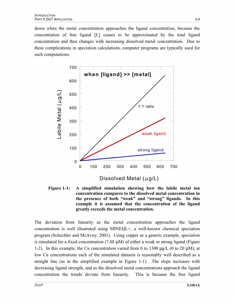
INTRODUCTION PART II DGT APPLICATION 1-3
INAP LORAX
down when the metal concentration approaches the ligand concentration, because the
concentration of free ligand [L] ceases to be approximated by the total ligand
concentration and thus changes with increasing dissolved metal concentration. Due to
these complications in speciation calculations, computer programs are typically used for
such computations.
0
100
200
300
400
500
600
700
0 100 200 300 400 500 600 700
when [ligand] >> [metal]
La
bile
Me
tal (
µg
/L)
Dissolved Metal ( µg/L)
weak ligand
strong ligand
1:1 ratio
Figure 1-1: A simplified simulation showing how the labile metal ion concentration compares to the dissolved metal concentration in the presence of both “weak” and “strong” ligands. In this example it is assumed that the concentration of the ligand greatly exceeds the metal concentration.
The deviation from linearity as the metal concentration approaches the ligand
concentration is well illustrated using MINEQL+, a well-known chemical speciation
program (Schechler and McAvoy, 2001). Using copper as a generic example, speciation
is simulated for a fixed concentration (7.88 µM) of either a weak or strong ligand (Figure
1-2). In this example, the Cu concentration varied from 0 to 1300 µg/L (0 to 20 µM); at
low Cu concentrations each of the simulated datasets is reasonably well described as a
straight line (as in the simplified example in Figure 1-1). The slope increases with
decreasing ligand strength, and as the dissolved metal concentrations approach the ligand
concentration the trends deviate from linearity. This is because the free ligand
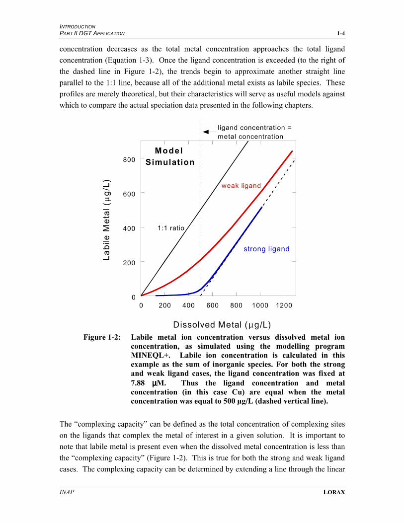
INTRODUCTION PART II DGT APPLICATION 1-4
INAP LORAX
concentration decreases as the total metal concentration approaches the total ligand
concentration (Equation 1-3). Once the ligand concentration is exceeded (to the right of
the dashed line in Figure 1-2), the trends begin to approximate another straight line
parallel to the 1:1 line, because all of the additional metal exists as labile species. These
profiles are merely theoretical, but their characteristics will serve as useful models against
which to compare the actual speciation data presented in the following chapters.
0
200
400
600
800
0 200 400 600 800 1000 1200
Model Simulation
La
bile
Me
tal (
µg
/L)
D issolved Metal (µg/L)
weak ligand
strong ligand
1:1 ratio
ligand concentration = metal concentration
Figure 1-2: Labile metal ion concentration versus dissolved metal ion
concentration, as simulated using the modelling program MINEQL+. Labile ion concentration is calculated in this example as the sum of inorganic species. For both the strong and weak ligand cases, the ligand concentration was fixed at 7.88 µµM. Thus the ligand concentration and metal concentration (in this case Cu) are equal when the metal concentration was equal to 500 µg/L (dashed vertical line).
The “complexing capacity” can be defined as the total concentration of complexing sites
on the ligands that complex the metal of interest in a given solution. It is important to
note that labile metal is present even when the dissolved metal concentration is less than
the “complexing capacity” (Figure 1-2). This is true for both the strong and weak ligand
cases. The complexing capacity can be determined by extending a line through the linear
INTRODUCTION PART II DGT APPLICATION 1-5
INAP LORAX
portion of the data, and is equal to the concentration at which this line intercepts the
x-axis (Figure 1-2). In subsequent chapters the term complexing capacity is used to refer
to the dissolved concentrations at which the ligand concentration is equal to the metal
concentrations (dashed vertical line in Figure 2-1).
Another approach, termed “Langmuir linearization”, is particularly useful for determining
complexing capacity (ligand concentration), when a single weak ligand is present. This
approach utilizes the fact that a plot of the ratio of labile to bound metal versus labile
metal yields a straight line, with a slope equal to 1/LT and an intercept of T
CondCuL LK '/
1. Thus,
from such a plot, the ligand concentration and strength can be determined. Because the
focus of this report is on intercomparisons of speciation techniques and not on
determinations of complexation capacity or ligand strength, Langmuir linearization is not
discussed in further detail.
1.3 Speciation Techniques
Speciation determinations were made in this study using two different techniques: 1)
DGT; and, 2) Anodic Stripping Voltammetry (ASV). These methods are discussed in
detail in Part I, Chapter 3. As a consequence, only a very brief summary of each
technique will be provided in this section.
In the DGT approach, metals are quantified using a ~4 cm-diameter disk-shaped device
that contains a filter membrane underlain by a polyacrylamide gel layer, consisting of
98% water, which is in turn underlain by a trace-metal-adsorbing gel-embedded resin
(Chelex). Metals diffuse from solution across the filter and gel layers to the underlying
resin, where metal sorption takes place. The resin only adsorbs free and kinetically-labile
metal ions. In ASV, the metal ion of interest is deposited on a mercury electrode via the
reduction of the metal to a metallic state and subsequent amalgamation with the mercury.
This is followed by a voltammetric scan, during which the mercury-bound metal is
oxidized and the current produced is determined. The identity of the metal is dictated by
the potential (voltage) of the peak, while the concentration is proportional to the current.
Each of these methods quantifies a fraction of the total metal concentration that includes
the free metal ion as well as those complexed species that dissociate to free metal ion at a
fast rate relative to the timescale of the measurement. These techniques can therefore
yield different results, in part due to differences in the timescales of the measurements.
For example, the timescale of the ASV method is on the order of ~0.1 seconds (Zhang
and Davison, 2000), while the timescale of the DGT method is on the order of ~10
minutes (the time required for diffusion of the metal species across the 0.8 mm-thick gel
layer; Zhang and Davison, 2000). Based on these considerations alone, the DGT method
INTRODUCTION PART II DGT APPLICATION 1-6
INAP LORAX
would be expected to quantify slowly-dissociating species better than the ASV method,
and thus the DGT approach would detect a larger fraction of the dissolved concentration
than would the ASV technique.
1.4 Experimental Design
In an attempt to better define metal species measured by existing techniques, laboratory
experiments were conducted to compare metal speciation data as determined by DGT,
ASV, and to a lesser extent ion-selective electrode (ISE) methods. In a second stage, the
speciation results were compared to a biological response using cultures of Daphnia
magna in defined ligand-bearing solutions. The latter component was conducted to
evaluate the various techniques as indicators of metal toxicity. Detailed experimental and
analytical procedures are described in Appendix A.
Copper (Cu), cadmium (Cd) and zinc (Zn) were the metals chosen for evaluation in this
study. Two well-characterized ligands, EDTA (Ethylenediaminetetraacetic acid) and
NTA (nitrilotriacetic acid), were used in the experiments. EDTA is widely used as a
metal chelator in industrial processes and has a strong affinity for a wide variety of
metals, while NTA is a well characterized moderately strong (weaker than EDTA) ligand.
Stability constants for EDTA and NTA complexes of Cu, Cd and Zn are provided in
Table 1-1.
Table 1-1: Stability Constants for Formations of Complexes
from Metals and Ligands (from Morel and Hering, 1993)1
Metal log K- EDTA log K- NTA
Cu 20.5 14.2
Cd 18.2 11.1
Zn 18.3 12.0
1Values given for zero ionic strength at 25ºC.
In addition to the experiments with synthetic solutions, the speciation of Cu and Cd was
carried out using natural waters rich in dissolved organic carbon (DOC). This water was
collected from the Nicomekl River, a meandering stream that receives runoff from peat
bogs and agricultural lands in southern Greater Vancouver. Nicomekl River waters have
been previously shown to complex Cu (Lorax, unpublished data). In addition, bioassays
using the copepod Daphnia magna were conducted on the experimental solutions in
which the dissolved, DGT-detectable and ASV-detectable concentrations had been
determined.

International Network for Acid Preventi
2 Copper

2-1
2. Copper
Copper concentrations in surface waters are subject to considerable regulatory scrutiny
due to the known toxicity of the metal to aquatic organisms (Sunda et al., 1987; Kessler,
1986). Copper speciation, and hence toxicity, is strongly influenced by the presence of a
variety of ligands in natural waters. For example, natural organic molecules may form
strong complexes with copper, significantly reducing the concentration of labile Cu
species in natural waters (Xue and Sunda, 1997; Sunda and Huntsman, 1998; Coale and
Bruland, 1988; Playle, 1998; Croot et al., 2000).
Previous work has demonstrated that copper concentrations determined by DGT have the
potential to provide a valuable indication of Cu complexation by both EDTA and DOC-
rich waters (Lorax, unpublished data). Specifically, DGT-Cu concentrations were
observed to be significantly lower in the presence of these ligands as compared to
dissolved concentrations (i.e., as determined following 0.45 µm filtration). The present
study expands on the previous work through a series of laboratory speciation and toxicity
studies. This chapter summarizes the data from the copper speciation intercomparison
experiments, as well as from a toxicity experiment. In brief, speciation intercomparisons
were carried out in the presence of: 1) EDTA, a strong, well-characterized ligand; 2)
NTA, a moderately strong (weaker than EDTA), well-characterized ligand; and 3)
Nicomekl River water, a DOC-rich freshwater stream previously shown to have a high
complexing affinity for copper. Experimental and analytical conditions for the
experiments are listed in Appendix A.
2.1 Experiments with EDTA
The aim of the experiments using EDTA as a ligand was to assess the effect of a known
strong ligand on the speciation of copper as measured by both ASV and DGT. In this
experiment, multiple solutions containing 1.47 mg/L EDTA (3.94 µM) had varying
amounts of Cu added to generate dissolved Cu concentrations ranging from 0-500 µg/L
(0 to 7.7 µM). These solutions were prepared using “moderately hard water”
(Appendix A).
Labile Cu concentrations as determined by DGT and ASV are plotted against dissolved
concentration in Figure 2-1. A theoretical 1:1 slope in Figure 2-1 represents the
relationship that would be expected in the absence of a ligand (i.e., labile Cu = dissolved
Cu). The line that forms the boundary between the shaded and un-shaded areas in Figure
2-1 represents the concentration of Cu that equals the complexing capacity of the EDTA.
The shaded area therefore represents concentrations of Cu in excess of the ligand, where

COPPER PART II DGT APPLICATION 2-2
INAP LORAX
added Cu would be expected to be in labile form. The theoretical distribution of labile
Cu (calculated as the sum of inorganic species) versus dissolved Cu in the presence of
EDTA, as determined by the geochemical speciation model MINEQL+ (version 4.5;
Appendix A), is also presented in Figure 2-1.
0
50
100
150
200
250
0 100 200 300 400 500
"L
abil
e" C
u (
µµg/
L)
Dissolved Cu (µµg/L)
DGT
ASV
MINEQL+
[Cu] > [ligand]
Cu + EDTA
1:1
Figure 2-1: DGT-Cu and ASV-Cu concentrations versus dissolved Cu in the
presence of EDTA. Also shown is the theoretical 1:1 slope for labile versus dissolved Cu in the absence of a ligand and the labile Cu concentration in the presence of EDTA as predicted by MINEQL+ (version 4.5).
DGT-Cu concentrations were below or close to detection limits (0.05 µg/L) in the
presence of excess EDTA (un-shaded area in Figure 2-1). Once the complexing capacity
of the EDTA was exceeded (shaded area in Figure 2-1), the concentration of labile and
dissolved Cu approximates a 1:1 slope, suggesting that all Cu was present in labile form.
The DGT data are in good agreement with the theoretical distribution of labile Cu as
calculated by MINEQL+ (Figure 2-1), although high DGT Cu blanks prevented a
rigorous intercomparison in this concentration range. These data indicate that DGT-Cu
concentrations provide a realistic measure of labile Cu concentrations in the presence of a
strong ligand.
ASV-Cu concentrations are higher than both DGT-Cu concentrations and those predicted
by MINEQL+ in solutions where the dissolved Cu content approaches and exceeds the
complexing capacity of EDTA (Figure 2-1). Once the complexing capacity of EDTA is
exceeded (shaded area in Figure 2-1), dissolved versus labile Cu concentrations as

COPPER PART II DGT APPLICATION 2-3
INAP LORAX
determined by ASV approximate a 1:1 slope, indicating that Cu added beyond the
complexing-capacity threshold was in labile form.
Generally, both ASV-Cu and DGT-Cu concentrations were significantly lower than
dissolved Cu concentrations, as would be expected in the presence of a strong ligand such
as EDTA. Both methods demonstrate that once the complexing capacity of EDTA has
been exceeded, all Cu added is labile. The main difference in assays of labile Cu by the
two methods occurred in solutions where the complexing capacity of EDTA was
approached (ligand > Cu). When this condition is established, measured ASV-Cu
concentrations were significantly higher than those determined by DGT-Cu or predicted
by MINEQL+. The reason for the “overestimation” of labile Cu as determined by ASV
in the presence of EDTA is not obvious; it is unlikely to be due to kinetic effects, as the
solutions were prepared at least 15 hours before the ASV determinations commenced.
Note that in all model runs, the “labile” fraction predicted by MINEQL+ in all model
runs is assumed to include all inorganically complexed Cu, not just Cu2+
. Furthermore,
in all MINEQL+ model runs, Cu mineral precipitation was turned off (see Appendix A).
MINEQL+ predicted precipitation of Cu-containing minerals at high Cu concentrations,
but such precipitation was not observed, hence it was not permitted in the model runs.
This observation can be explained either by slow precipitation kinetics or inaccuracies in
the MINEQL+ database.
2.2 Experiments with NTA
The aim of the NTA experiment was to determine Cu speciation in the presence of a
well-characterized ligand that is substantially weaker than EDTA. In this experiment,
NTA was added to the solutions at a concentration of 2.17 mg/L (7.88 µM), while Cu
was added to yield dissolved concentrations between 0 and ~900 µg/L (0 to 14 µM).
DGT-Cu and ASV-Cu concentrations, as well as the theoretical distribution of labile Cu
in the presence of NTA, as predicted by MINEQL+, are presented in Figure 2-2.
ASV-Cu concentrations were below the detection limit for solutions in which NTA was
well in excess of Cu concentrations (Figure 2-2). ASV-Cu increased in solutions
approaching the complexing capacity of NTA, although this increase was observed when
there was still an excess of NTA. Labile Cu concentrations predicted by MINEQL+ were
lower than the ASV results and much closer to the ISE results (Figure 2-2).
The DGT-Cu concentrations in the presence of NTA are consistently higher than ASV
and predicted (MINEQL+) concentrations. At Cu levels >~300 µg/L, the trend of the
DGT-Cu versus dissolved Cu data is near linear and approximates a 1:1 slope. DGT-Cu
values are however approximately 30% lower than dissolved concentrations (Figure 2-2).
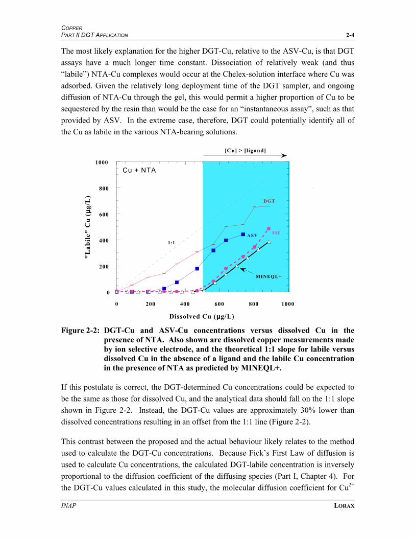
COPPER PART II DGT APPLICATION 2-4
INAP LORAX
The most likely explanation for the higher DGT-Cu, relative to the ASV-Cu, is that DGT
assays have a much longer time constant. Dissociation of relatively weak (and thus
“labile”) NTA-Cu complexes would occur at the Chelex-solution interface where Cu was
adsorbed. Given the relatively long deployment time of the DGT sampler, and ongoing
diffusion of NTA-Cu through the gel, this would permit a higher proportion of Cu to be
sequestered by the resin than would be the case for an “instantaneous assay”, such as that
provided by ASV. In the extreme case, therefore, DGT could potentially identify all of
the Cu as labile in the various NTA-bearing solutions.
0
200
400
600
800
1000
0 200 400 600 800 1000
"L
abil
e" C
u (
µµg/
L)
Dissolved Cu (µµg/L)
DGT
ASV
MINEQL+
1:1
[Cu] > [ligand]
Cu + NTA
ISE
Figure 2-2: DGT-Cu and ASV-Cu concentrations versus dissolved Cu in the presence of NTA. Also shown are dissolved copper measurements made by ion selective electrode, and the theoretical 1:1 slope for labile versus dissolved Cu in the absence of a ligand and the labile Cu concentration in the presence of NTA as predicted by MINEQL+.
If this postulate is correct, the DGT-determined Cu concentrations could be expected to
be the same as those for dissolved Cu, and the analytical data should fall on the 1:1 slope
shown in Figure 2-2. Instead, the DGT-Cu values are approximately 30% lower than
dissolved concentrations resulting in an offset from the 1:1 line (Figure 2-2).
This contrast between the proposed and the actual behaviour likely relates to the method
used to calculate the DGT-Cu concentrations. Because Fick’s First Law of diffusion is
used to calculate Cu concentrations, the calculated DGT-labile concentration is inversely
proportional to the diffusion coefficient of the diffusing species (Part I, Chapter 4). For
the DGT-Cu values calculated in this study, the molecular diffusion coefficient for Cu2+
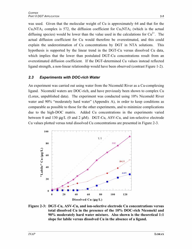
COPPER PART II DGT APPLICATION 2-5
INAP LORAX
was used. Given that the molecular weight of Cu is approximately 64 and that for the
Cu3NTA2 complex is 572, the diffusion coefficient for Cu3NTA2 (which is the actual
diffusing species) would be lower than the value used in the calculations for Cu2+
. The
actual diffusion coefficient for Cu would therefore be overestimated, and this could
explain the underestimation of Cu concentrations by DGT in NTA solutions. This
hypothesis is supported by the linear trend in the DGT-Cu versus dissolved Cu data,
which implies that the lower than postulated DGT-Cu concentrations result from an
overestimated diffusion coefficient. If the DGT-determined Cu values instead reflected
ligand strength, a non-linear relationship would have been observed (contrast Figure 1-2).
2.3 Experiments with DOC-rich Water
An experiment was carried out using water from the Nicomekl River as a Cu-complexing
ligand. Nicomekl waters are DOC-rich, and have previously been shown to complex Cu
(Lorax, unpublished data). The experiment was conducted using 10% Nicomekl River
water and 90% “moderately hard water” (Appendix A), in order to keep conditions as
comparable as possible to those for the other experiments, and to minimize complications
due to the high-DOC matrix. Added Cu concentrations in the experiments varied
between 0 and 130 µg/L (0 and 2 µM). DGT-Cu, ASV-Cu, and ion-selective electrode
Cu values plotted versus total dissolved Cu concentrations are presented in Figure 2-3.
0
20
40
60
80
100
0 20 40 60 80 100 120
"L
abil
e" C
u (
µµg/
L)
Dissolved Cu (µµg/L)
ASV
DGT
ISE
1:1
Figure 2-3: DGT-Cu, ASV-Cu, and ion-selective electrode Cu concentrations versus
total dissolved Cu in the presence of the 10% DOC-rich Nicomekl and 90% moderately hard water mixture. Also shown is the theoretical 1:1 slope for labile versus dissolved Cu in the absence of a ligand.
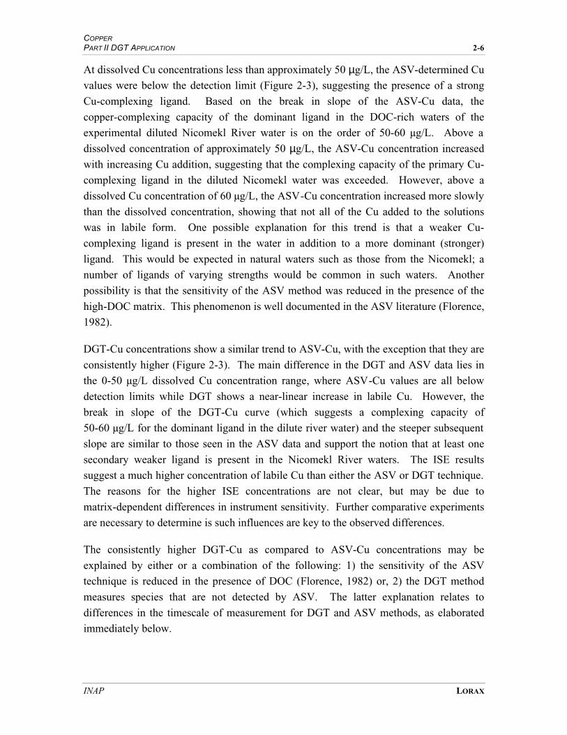
COPPER PART II DGT APPLICATION 2-6
INAP LORAX
At dissolved Cu concentrations less than approximately 50 µg/L, the ASV-determined Cu
values were below the detection limit (Figure 2-3), suggesting the presence of a strong
Cu-complexing ligand. Based on the break in slope of the ASV-Cu data, the
copper-complexing capacity of the dominant ligand in the DOC-rich waters of the
experimental diluted Nicomekl River water is on the order of 50-60 µg/L. Above a
dissolved concentration of approximately 50 µg/L, the ASV-Cu concentration increased
with increasing Cu addition, suggesting that the complexing capacity of the primary Cu-
complexing ligand in the diluted Nicomekl water was exceeded. However, above a
dissolved Cu concentration of 60 µg/L, the ASV-Cu concentration increased more slowly
than the dissolved concentration, showing that not all of the Cu added to the solutions
was in labile form. One possible explanation for this trend is that a weaker Cu-
complexing ligand is present in the water in addition to a more dominant (stronger)
ligand. This would be expected in natural waters such as those from the Nicomekl; a
number of ligands of varying strengths would be common in such waters. Another
possibility is that the sensitivity of the ASV method was reduced in the presence of the
high-DOC matrix. This phenomenon is well documented in the ASV literature (Florence,
1982).
DGT-Cu concentrations show a similar trend to ASV-Cu, with the exception that they are
consistently higher (Figure 2-3). The main difference in the DGT and ASV data lies in
the 0-50 µg/L dissolved Cu concentration range, where ASV-Cu values are all below
detection limits while DGT shows a near-linear increase in labile Cu. However, the
break in slope of the DGT-Cu curve (which suggests a complexing capacity of
50-60 µg/L for the dominant ligand in the dilute river water) and the steeper subsequent
slope are similar to those seen in the ASV data and support the notion that at least one
secondary weaker ligand is present in the Nicomekl River waters. The ISE results
suggest a much higher concentration of labile Cu than either the ASV or DGT technique.
The reasons for the higher ISE concentrations are not clear, but may be due to
matrix-dependent differences in instrument sensitivity. Further comparative experiments
are necessary to determine is such influences are key to the observed differences.
The consistently higher DGT-Cu as compared to ASV-Cu concentrations may be
explained by either or a combination of the following: 1) the sensitivity of the ASV
technique is reduced in the presence of DOC (Florence, 1982) or, 2) the DGT method
measures species that are not detected by ASV. The latter explanation relates to
differences in the timescale of measurement for DGT and ASV methods, as elaborated
immediately below.
COPPER PART II DGT APPLICATION 2-7
INAP LORAX
The effective analytical time of speciation measurements is proportional to the square of
the distance that the analyte must diffuse between the bulk solution and the measurement
interface. The diffusion distance for ASV is on the order of 10 µm in a typical well-
stirred solution (Zhang and Davison, 2000), while it is on the order of 1 mm (1000 µm)
for a DGT device. For ASV, the effective measurement time translates to approximately
0.1 seconds, while for DGT it is closer to 13.5 minutes, roughly 104 times as long (Zhang
and Davison, 2000). Thus, the ASV technique will only detect species with rapid
dissociation kinetics (i.e. those that can dissociate within 0.1 seconds). Such dissociation
rates are limited to weak inorganic complexes. In contrast, the DGT technique will detect
both rapidly dissociating species and those with much slower dissociation kinetics (i.e.
those that dissociate within ~10-15 minutes). The DGT approach would thus be expected
to detect less labile species, because there is considerably more time for such complexes
to dissociate during diffusion. Based on this discussion, the labile fraction as determined
by DGT would include complexes that dissociate more slowly than those measured by
ASV. This suggestion is consistent with the higher DGT-Cu concentrations (compared to
ASV-Cu) observed in the NTA and DOC speciation experiments. DGT therefore
provides a more liberal estimate of labile metal species in natural waters than ASV.
2.3.1 Speciation and Toxicity Comparisons
The same diluted Nicomekl River waters that were analyzed by all three speciation
methods were also used in a 48-hour acute lethality bioassay on the copepod D. magna.
Thus, direct comparisons can be made between the speciation and mortality data to assess
which speciation technique provides the best indication of the bioavailability of copper to
this organism. ASV-Cu, DGT-Cu and ISE-Cu concentrations plotted against dissolved
Cu concentrations and toxicity data from D. magna bioassays are presented in Figure 2-4.
The onset of mortality for D. magna occurred at dissolved (0.45 µm filtered) Cu
concentrations of approximately 30 µg/L, with an abrupt increase in mortality being
observed at a dissolved Cu concentration of ~60 µg/L (Figure 2-4). These toxicity data
are consistent with DGT and ASV results which indicated that the complexing capacity
of the dominant ligand was 50-60 µg/L.
ASV-Cu concentrations were below detection limits at concentrations in which a 10%
mortality rate for D. magna was observed (Figure 2-4). Over the 10 to 70% mortality
range, ASV-Cu increased from 0 to only ~ 3 µg/L. The low ASV-Cu concentration
measured in a solution with 70% mortality demonstrates that the ASV technique
underestimates toxicity to D. magna. Underestimation of Cu toxicity by the ASV
technique has been observed elsewhere (Florence, 1982). By contrast, DGT-Cu values of
approximately 10 µg/L were observed in the lower range of D. magna mortality (10%).
COPPER PART II DGT APPLICATION 2-8
INAP LORAX
These increased to approximately 15 µg/L as mortality increased to 70% (Figure 2-4).
The DGT-determined Cu values therefore demonstrated better correlation with the
observed toxicological effects than did the ASV-Cu concentrations. However, only 10%
mortality was observed at DGT-Cu concentrations as high as 10.5 µg/L Cu, a
concentration essentially equivalent to the dissolved Cu LC50 (10.8 µg/L) in the absence
of any ligand. This suggests that the DGT approach may overestimate Cu toxicity to D.
magna.
0
10
20
30
40
50
60
0 20 40 60 80 100 120
"L
abil
e" C
u ( µµ
g/L
)
D issolved Cu (µµ g/L)
0% mortality
10%up to
70%
100% mortality
Bioassay in Nicomekl
ASV
DGT
D. magna
Figure 2-4: DGT-Cu, ASV-Cu, and ISE-Cu concentrations versus dissolved Cu and D. magna toxicity data in the presence of the 10% DOC-rich Nicomekl and 90% moderately hard water mixture.
LC50 values for dissolved Cu in moderately hard water (no ligand) and for DGT, ASV
and dissolved Cu in the Nicomekl and moderately hard water mixture (with ligand) are
presented in Figure 2-5. The dissolved Cu LC50 was 49 µg/L in the presence of the
Nicomekl/moderately hard water mixture, considerably higher than the dissolved Cu
LC50 of 10.8 µg/L in moderately hard water with no added DOC, demonstrating the
effect of Cu complexation on the toxicity of the Nicomekl water mixture. These data
reinforce the now well-known limitations of "total dissolved Cu" concentrations as an
indicator of toxicity to aquatic organisms. By contrast, the DGT-Cu LC50 of 13.3 µg/L
was much closer to the dissolved Cu determined in the absence of added ligand (Cu LC50
of 10.8 µg/L). The close agreement between the LC50 for labile Cu in the test solution
with no ligand and that for the labile Cu as determined by DGT in the presence of at least
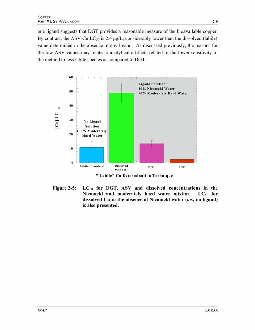
COPPER PART II DGT APPLICATION 2-9
INAP LORAX
one ligand suggests that DGT provides a reasonable measure of the bioavailable copper.
By contrast, the ASV-Cu LC50 is 2.4 µg/L, considerably lower than the dissolved (labile)
value determined in the absence of any ligand. As discussed previously, the reasons for
the low ASV values may relate to analytical artifacts related to the lower sensitivity of
the method to less labile species as compared to DGT.
0
10
20
30
40
50
60
[Cu
] L
C
Ligand Solution:10% Nicomekl Water90% M oderately Hard Water
No LigandSolution:
100% M oderatelyHard Water
Labile=Dissolved Dissolved0.45 um
DGT ASV
" Labile" Cu Determination Technique
50
Figure 2-5: LC50 for DGT, ASV and dissolved concentrations in the Nicomekl and moderately hard water mixture. LC50 for dissolved Cu in the absence of Nicomekl water (i.e., no ligand) is also presented.

International Network for Acid Preventi
3 Cadmium
3-1
3. Cadmium
Although cadmium speciation in natural waters is not as well understood as that of
copper, a variety of studies have demonstrated that complexation of Cd can be significant.
For example, natural organic molecules have been shown in seawater to form strong
complexes with cadmium, strongly reducing the concentration of “labile” Cd species
(Kozelka and Bruland, 1998; Wells et al., 1998).
This chapter summarizes the data from the speciation intercomparision experiments
carried out with cadmium in the presence of: 1) EDTA, a strong, well-characterized
ligand, and 2) NTA (nitrilotriacetic acid), a moderately strong, well-characterized ligand.
Experimental and analytical conditions for the experiments are listed in Appendix A.
3.1 Experiments with EDTA
As for copper, the intent of using EDTA was to assess experimentally the impact of a
known “strong” ligand on Cd speciation. In the experiment, multiple solutions containing
3.31 mg/L EDTA (8.89 µM) had varying amounts of Cd added, generating solutions with
concentrations ranging from 0-1600 µg/L (0 to 14 µM). The solutions were prepared
using “moderately hard water” (Appendix A).
Labile Cd concentrations as determined by DGT and ASV are plotted against dissolved
concentration in Figure 3-1. The theoretical 1:1 slope in Figure 3-1 represents the
relationship that would be expected in the absence of a ligand (i.e., labile Cd = dissolved
Cd). The boundary between the shaded and un-shaded areas in Figure 3-1 represents the
concentration of Cd that equals the complexing capacity of the EDTA. The shaded area
therefore represents concentrations of Cd in excess of the ligand, where added Cd would
be expected to be in labile form. The theoretical distribution of labile Cd versus
dissolved Cd as determined by MINEQL+ (version 4.5; Appendix A), is also shown.
Over the full range of total dissolved Cd concentrations in this experiment, the labile Cd
levels as determined by ASV are in reasonable agreement with those predicted by
MINEQL+ (version 4.5; Figure 3-1). These data suggest that ASV-Cu concentrations
provide a realistic measure of labile Cd concentrations in the presence of a strong ligand.
However, it must be noted that the correlation between the MINEQL+-predicted and the
measured "labile" Cd values was achieved only by suppressing the precipitation of otavite
(CdCO3) during the MINEQL+ model runs. Without such suppression, no significant
concentration of labile Cd species would have been predicted by MINEQL+ at high
concentrations of added Cd. Precipitation of otavite was also predicted by PHREEQC
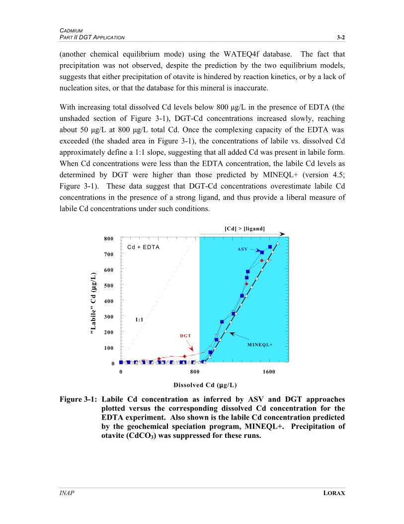
CADMIUM PART II DGT APPLICATION 3-2
INAP LORAX
(another chemical equilibrium mode) using the WATEQ4f database. The fact that
precipitation was not observed, despite the prediction by the two equilibrium models,
suggests that either precipitation of otavite is hindered by reaction kinetics, or by a lack of
nucleation sites, or that the database for this mineral is inaccurate.
With increasing total dissolved Cd levels below 800 µg/L in the presence of EDTA (the
unshaded section of Figure 3-1), DGT-Cd concentrations increased slowly, reaching
about 50 µg/L at 800 µg/L total Cd. Once the complexing capacity of the EDTA was
exceeded (the shaded area in Figure 3-1), the concentrations of labile vs. dissolved Cd
approximately define a 1:1 slope, suggesting that all added Cd was present in labile form.
When Cd concentrations were less than the EDTA concentration, the labile Cd levels as
determined by DGT were higher than those predicted by MINEQL+ (version 4.5;
Figure 3-1). These data suggest that DGT-Cd concentrations overestimate labile Cd
concentrations in the presence of a strong ligand, and thus provide a liberal measure of
labile Cd concentrations under such conditions.
0
100
200
300
400
500
600
700
800
0 800 1600
"L
abil
e" C
d (
µµg/
L)
Dissolved Cd (µµg/L)
ASV
DGT
M INEQL+
1:1
[Cd] > [ligand]
Cd + EDTA
Figure 3-1: Labile Cd concentration as inferred by ASV and DGT approaches
plotted versus the corresponding dissolved Cd concentration for the EDTA experiment. Also shown is the labile Cd concentration predicted by the geochemical speciation program, MINEQL+. Precipitation of otavite (CdCO3) was suppressed for these runs.
CADMIUM PART II DGT APPLICATION 3-3
INAP LORAX
Bioassays were carried out in solutions containing 0.034 mg/L EDTA (0.09 µM) and
0-21 µg/L (0-0.19 µM) total dissolved Cd. However, no mortality was observed in any of
the solutions; hence none of these results are presented. The results do strongly imply,
however, that the acute toxicity threshold for Daphnia magna with respect to cadmium is
higher than 21 µg/L total Cd in "moderately hard water".
3.2 Experiments with NTA
The intent of using NTA as a ligand was to determine Cd speciation in the presence of a
well-characterized ligand that is substantially weaker than EDTA. In the experiment
NTA was added to the solutions at a concentration of 2.04 mg/L (7.5 µM), while Cd was
added at concentrations ranging from 0 to ~930 µg/L (0 to 8.3 µM).
ASV-Cd concentrations were less than half those determined by DGT in solutions in
which NTA was well in excess of total dissolved Cd contents (Figure 3-2). ASV-Cd
increased quasi-exponentially in solutions as the complexing capacity of NTA was
approached, while the DGT-Cd vs. dissolved Cd relationship remained linear across the
analytical range (Figure 3-2). The ASV-Cd concentrations are within a factor of two of
the MINEQL+ predictions, which is reasonable agreement. However, the DGT-Cd
concentrations are much higher.
The most likely explanation for the higher DGT-Cd, relative to the ASV-Cd, is that DGT
assays have a much longer time constant. Dissociation of relatively weak (and thus
“labile”) NTA-Cd complexes would occur at the Chelex-solution interface where Cd was
adsorbed. Given the relatively long deployment time of the DGT sampler, and ongoing
diffusion of NTA-Cd through the gel, this would permit a higher proportion of Cd to be
sequestered by the resin than would be the case for an “instantaneous assay”, such as that
provided by ASV. In the extreme case, therefore, DGT could potentially identify all of the
Cd as labile in the various NTA-bearing solutions. A similar suggestion was made for
copper in the preceding chapter. If this postulate is correct, the DGT-determined Cd
concentrations should be expected to be the same as those for total dissolved Cd, and the
analytical data should fall on the 1:1 slope shown in Figure 3-2. Instead, and as was
observed for Cu (Figure 2-2), the DGT-Cd values are approximately 30% lower than
dissolved concentrations resulting in an offset from the 1:1 line (Figure 3-2).
As discussed for copper in section 2.2, the difference between the proposed and the actual
behaviour likely relates to the use of Fick’s First Law in calculating the DGT-labile
concentration, which is inversely proportional to the diffusion coefficient of the diffusing

CADMIUM PART II DGT APPLICATION 3-4
INAP LORAX
species (Part I, Chapter 4). For the DGT-Cd values calculated in this study, the molecular
diffusion coefficient for Cd2+
was used. Given that the molecular weight of Cd is
approximately 112 and that for the Cd3(NTA)2 complex is 713, Cd3(NTA)2, the actual
diffusing species, would diffuse more slowly than Cd2+
. This could explain the
underestimation of Cd concentrations by DGT in NTA solutions. This hypothesis is
supported by the linear trend in the DGT-Cd versus dissolved Cd data, which implies that
the lower than postulated calculated DGT-Cd concentrations result from an overestimated
diffusion coefficient.
0
100
200
300
400
500
600
700
800
0 400 800
"L
abil
e" C
d (
µµg/
L)
Dissolved Cd (µµg/L)
ASV
DGT
MINEQL+
1:1Cd + NTA
[Cd] > [ligand]
Figure 3-2: Labile Cd concentration as inferred by the ASV and DGT approaches plotted versus the corresponding dissolved Cd concentration for the NTA experiment. Also shown is the labile Cd concentration predicted by the geochemical speciation program, MINEQL+. Precipitation of otavite (CdCO3) was suppressed for these runs.
It is worth noting that the stability constant for the Cu-NTA complex is three orders of
magnitude larger than that for the Cd-NTA complex (Table 1-1, and Morel and Hering,
1993). Hence, there should be a significant difference in the trends of labile Cu and Cd
versus the dissolved concentrations when NTA is present in excess, as is predicted by
MINEQL+. Comparison of the curves for MINEQL+ in Figures 2-2 and 3-2 illustrates
well the net result of the difference in the stability constants. However, this contrast did
not carry through to the actual DGT-based determinations of labile Cd and Cu. The DGT
approach consistently determined concentrations of both metals only one-third or so
lower than the dissolved values, while ASV yielded lower values. As noted above, we
CADMIUM PART II DGT APPLICATION 3-5
INAP LORAX
attribute this contrast to the longer timescale of the DGT measurement, a function of
diffusion through the gel layer. This probably leads to detection of more slowly
dissociating species (and hence higher measured concentrations) compared to ASV.
3.3 Nicomekl River Water
An additional experiment was conducted using Nicomekl River water as the metal-
complexing ligand. However, unlike the case for copper, zero complexation of Cd was
apparent in the ASV determinations. As a result, no DGT units were deployed, and no
data are presented.

International Network for Acid Preventi
4 Zinc
4-1
4. Zinc
As is the case for a copper and cadmium, a variety of studies have demonstrated that zinc
exists largely in complexed form in natural waters. For example, Zn in river water has
been shown to be significantly complexed, leading to a ~50% reduction in bioavailability
(Jansen et al, 1998). Furthermore, Zn in seawater has been shown to be largely
complexed by organic ligands, strongly reducing the concentration of “labile” zinc
species (Kozelka and Bruland, 1998; Wells et al., 1998). This chapter summarizes the
data from a Zn speciation intercomparison experiment that was carried out in the presence
of EDTA, as well as data from a bioassay carried out on D. magna. Experimental and
analytical conditions for the experiments are listed in Appendix A.
4.1 Experiments with EDTA
As for the other metals discussed in this report, the intent of using EDTA as a ligand was
to assess experimentally the impact of a known “strong” ligand on Zn speciation. In this
experiment, multiple solutions containing 8.56 mg/L EDTA (23 µM) had varying
amounts of Zn added to generate solutions with concentrations ranging from 0-2700 µg/L
(0 to 42 µM). The solutions were again prepared using “moderately hard water” (see
Appendix A).
Labile Zn concentrations as determined by DGT and ASV are plotted against total
dissolved concentration in Figure 4-1. The theoretical 1:1 slope in Figure 4-1 represents
the relationship that would be expected in the absence of a ligand. The boundary between
the shaded and un-shaded areas in Figure 4-1 represents the zinc concentration (~1500
µg/L) that equals the complexing capacity of the EDTA. The shaded area therefore
represents concentrations of Zn in excess of the ligand, where added metal would be
expected to be in labile form. The theoretical distribution of labile versus dissolved Zn in
the presence of EDTA, as predicted by MINEQL+ (Appendix A), is also shown in the
figure.
DGT-Zn concentrations in the presence of excess EDTA (the un-shaded area in
Figure 4-1) range from undetectable at zero added Zn2+
to ~110 µg/L at 1500 µg/L added
total dissolved zinc. Above the complexing capacity of the EDTA (the shaded area in
Figure 4-1), the slope of the labile vs. dissolved Zn relationship is ~1, implying that all
added zinc was present in labile form. DGT-Zn concentrations significantly exceed those
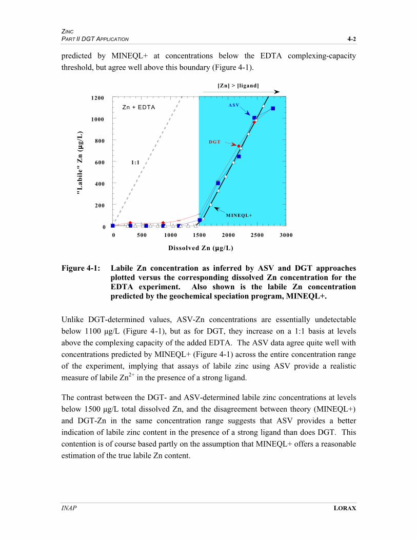
ZINC PART II DGT APPLICATION 4-2
INAP LORAX
predicted by MINEQL+ at concentrations below the EDTA complexing-capacity
threshold, but agree well above this boundary (Figure 4-1).
0
200
400
600
800
1000
1200
0 500 1000 1500 2000 2500 3000
"L
abil
e" Z
n (
µµg/
L)
Dissolved Zn (µµg/L)
ASV
D G T
M INEQL+
[Zn] > [ligand]
1:1
Zn + EDTA
Figure 4-1: Labile Zn concentration as inferred by ASV and DGT approaches plotted versus the corresponding dissolved Zn concentration for the EDTA experiment. Also shown is the labile Zn concentration predicted by the geochemical speciation program, MINEQL+.
Unlike DGT-determined values, ASV-Zn concentrations are essentially undetectable
below 1100 µg/L (Figure 4-1), but as for DGT, they increase on a 1:1 basis at levels
above the complexing capacity of the added EDTA. The ASV data agree quite well with
concentrations predicted by MINEQL+ (Figure 4-1) across the entire concentration range
of the experiment, implying that assays of labile zinc using ASV provide a realistic
measure of labile Zn2+
in the presence of a strong ligand.
The contrast between the DGT- and ASV-determined labile zinc concentrations at levels
below 1500 µg/L total dissolved Zn, and the disagreement between theory (MINEQL+)
and DGT-Zn in the same concentration range suggests that ASV provides a better
indication of labile zinc content in the presence of a strong ligand than does DGT. This
contention is of course based partly on the assumption that MINEQL+ offers a reasonable
estimation of the true labile Zn content.

ZINC PART II DGT APPLICATION 4-3
INAP LORAX
Bioassay experiments support the conclusion that ASV and DGT assays provide a
reasonable estimation of bioavailable zinc in the presence of EDTA, a strong ligand. As
for copper (Chapter 2) the toxicity of zinc to Daphnia magna was determined, via
standard bioassays that were carried out in the same solutions in which the DGT units
were deployed. An aliquot from each solution was also taken for ASV determinations.
The bioassay results support the observation that Zn is significantly complexed by EDTA.
No mortality was observed until the dissolved Zn concentration exceeded the EDTA
concentration. Indeed, total dissolved zinc values on the order of 2000 µg/L were
required to produce significant mortality in the presence of 8.56 µM EDTA (LC50 = 2020
µg/L), as summarized in Figure 4-2. DGT assays and ASV analyses of the same solutions
yielded LC50 concentrations some four-fold lower (~500 µg/L; Figure 4-2). These
operationally-defined values for "labile metal" illustrate the effectiveness of EDTA as a
chelating agent. More importantly, bioassays carried out by B.C. Research using D.
magna and EDTA-free “moderately hard water” yielded an LC50 of 575±200 µg/L
dissolved zinc. This result is statistically indistinguishable from the LC50 values
determined in the presence of EDTA by both DGT and ASV (Figure 4-2). Such common
behaviour suggests that both the ASV and the DGT methods yield reasonable
determinations of “labile” Zn when Zn concentrations exceed the complexing capacity of
a “strong” ligand.
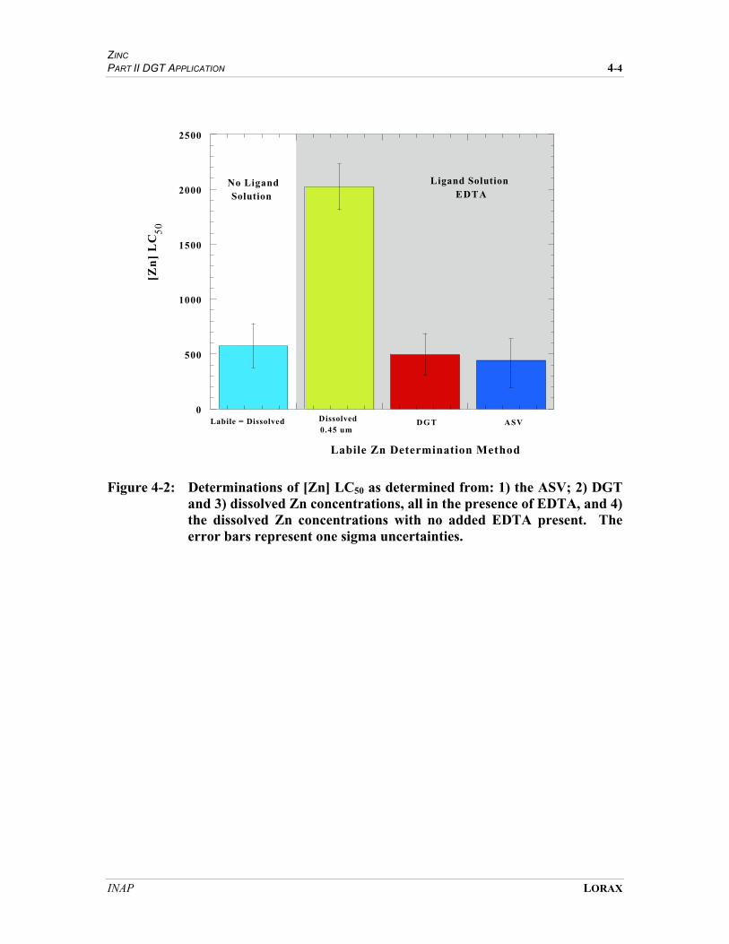
ZINC PART II DGT APPLICATION 4-4
INAP LORAX
0
500
1000
1500
2000
2500
[Zn
] L
C5
0
Labile = Dissolved Dissolved0.45 um
DGT ASV
Labile Zn Determination Method
Ligand SolutionEDTA
No LigandSolution
Figure 4-2: Determinations of [Zn] LC50 as determined from: 1) the ASV; 2) DGT and 3) dissolved Zn concentrations, all in the presence of EDTA, and 4) the dissolved Zn concentrations with no added EDTA present. The error bars represent one sigma uncertainties.

International Network for Acid Preventi
5 Summary and Conclusions

5-1
5. Summary and Conclusions
The experiments discussed in this report have illustrated that both Diffusive Gels in Thin
Films (DGT) and Anodic Stripping Voltammetry (ASV) can provide estimates of labile
Cu, Cd and Zn in natural waters in which both strong and weak complexing agents are
present. Furthermore, bioassays show that the DGT technique provides an accurate
measure of the Cu and Zn available to the water flea Daphnia magna. A number of
caveats exist, however, and these are enumerated in the following key conclusions.
1. In the presence of an excess of the strong ligand EDTA (ethylenediaminetetraacetic
acid), labile Cu, Cd and Zn concentrations as measured by both DGT and ASV
approaches are substantially lower than total dissolved metal concentrations. However,
DGT-labile concentrations are consistently higher than those assayed using ASV.
Chemical equilibrium modeling (using MINEQL+) of Cu- and Zn-containing solutions
suggests the DGT technique overestimates the labile concentration while the ASV
approach provides a more reasonable estimate.
2. When total dissolved metal concentrations exceed the complexing capacity of the
EDTA in solution, both methods provide accurate determinations of the labile
concentration, suggesting that both approaches can quantify metal complexing capacity in
the presence of strong ligands.
3. In the presence of an excess of the moderately strong ligand NTA (nitrilotriacetic acid),
labile Cu and Cd concentrations as determined by ASV are substantially lower than the
dissolved metal concentrations. DGT, by contrast, measures concentrations only ~25%
lower than total dissolved levels. The difference is attributed to two factors: (a) the
Chelex resin used in the DGT samplers is a strong complexing agent, and readily adsorbs
free metal ions, maintaining a concentration gradient between the resin-gel interface and
the bulk solution; (b) ASV samples the solution on a timescale of a fraction of a second,
whereas DGT samples over ten or more minutes. Thus, the much greater time required
for the metal to diffuse from solution to detection surface in the DGT approach permits
dissociation of more slowly dissociating complexes and uptake of freed metal ions and
thus leads to detection of a larger "labile" concentration by the DGT technique.
4. As for the strong ligand, EDTA, when the metal concentrations exceed the complexing
capacity of the added weak ligand NTA, both ASV and DGT provide accurate
determinations of the labile metal concentration.
SUMMARY AND CONCLUSIONS PART II DGT APPLICATION 5-2
INAP LORAX
5. Data obtained from experiments using natural waters suggest the presence of both
strong and weak ligands. Under such conditions DGT and ASV delivered similar results.
In a dilute solution of DOC-rich Nicomekl River water (90% "moderately hard water"
and 10% river water), ASV-labile Cu concentrations were undetectable (<0.05 µg/L)
when the dissolved Cu concentration was below ~50 µg/L (0.8 µM), indicating the
presence of a ligand with a high affinity for Cu. At higher dissolved concentrations the
ASV-labile concentration increased, but not as quickly as the dissolved concentration,
suggesting the presence of a weaker ligand at a concentration above 0.8 µΜ. The DGT-
labile concentrations were consistently ~30% of the dissolved concentrations,
considerably higher than the ASV-labile values, probably reflecting the two factors
summarized in point 3 above.
6. Bioassays for Cu and Zn using Daphnia magna offer insight as to which method
provides a better measure of metal availability to biota. In the Cu-amended mixture of
"moderately hard water" and Nicomekl River water, ASV severely underestimated
availability to D. magna while DGT predicted within 30% the LC50 concentration of
copper. In Zn-amended EDTA-containing solution, both the ASV and DGT approaches
yielded reasonable estimates of metal availability. These data are consistent with the
suggestion that the ASV approach provides a measure of “free” metal ion, but fails to
detect an additional fraction of “labile” metal that is available to biota. The DGT
approach detects this additional “labile” fraction, although it appears to slightly
overestimate the concentration.

International Network for Acid Preventi
Appendix A: Experimental Design
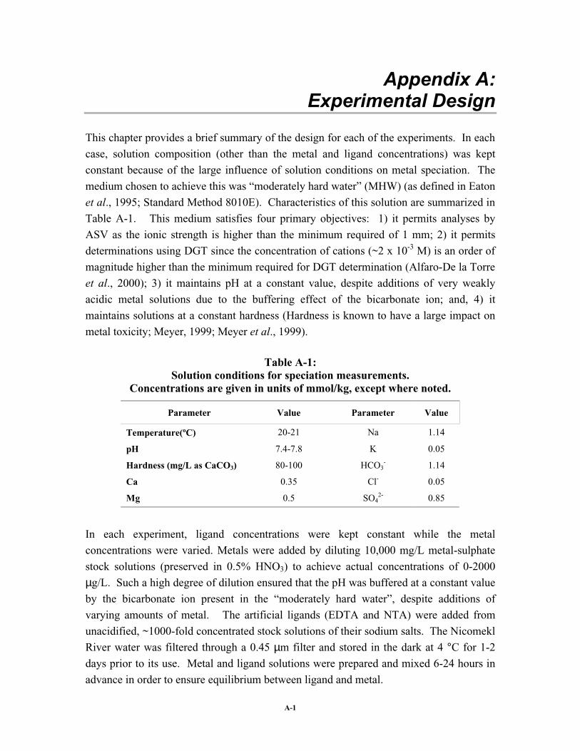
A-1
Appendix A: Experimental Design
This chapter provides a brief summary of the design for each of the experiments. In each
case, solution composition (other than the metal and ligand concentrations) was kept
constant because of the large influence of solution conditions on metal speciation. The
medium chosen to achieve this was “moderately hard water” (MHW) (as defined in Eaton
et al., 1995; Standard Method 8010E). Characteristics of this solution are summarized in
Table A-1. This medium satisfies four primary objectives: 1) it permits analyses by
ASV as the ionic strength is higher than the minimum required of 1 mm; 2) it permits
determinations using DGT since the concentration of cations (~2 x 10⁻³
M) is an order of
magnitude higher than the minimum required for DGT determination (Alfaro-De la Torre
et al., 2000); 3) it maintains pH at a constant value, despite additions of very weakly
acidic metal solutions due to the buffering effect of the bicarbonate ion; and, 4) it
maintains solutions at a constant hardness (Hardness is known to have a large impact on
metal toxicity; Meyer, 1999; Meyer et al., 1999).
Table A-1: Solution conditions for speciation measurements.
Concentrations are given in units of mmol/kg, except where noted.
Parameter Value Parameter Value
Temperature(ºC) 20-21 Na 1.14
pH 7.4-7.8 K 0.05
Hardness (mg/L as CaCO3) 80-100 HCO3- 1.14
Ca 0.35 Cl- 0.05
Mg 0.5 SO42-
0.85
In each experiment, ligand concentrations were kept constant while the metal
concentrations were varied. Metals were added by diluting 10,000 mg/L metal-sulphate
stock solutions (preserved in 0.5% HNO3) to achieve actual concentrations of 0-2000
µg/L. Such a high degree of dilution ensured that the pH was buffered at a constant value
by the bicarbonate ion present in the “moderately hard water”, despite additions of
varying amounts of metal. The artificial ligands (EDTA and NTA) were added from
unacidified, ~1000-fold concentrated stock solutions of their sodium salts. The Nicomekl
River water was filtered through a 0.45 µm filter and stored in the dark at 4 °C for 1-2
days prior to its use. Metal and ligand solutions were prepared and mixed 6-24 hours in
advance in order to ensure equilibrium between ligand and metal.
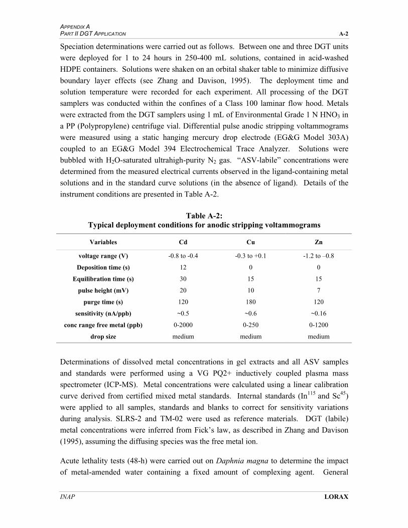
APPENDIX A PART II DGT APPLICATION A-2
INAP LORAX
Speciation determinations were carried out as follows. Between one and three DGT units
were deployed for 1 to 24 hours in 250-400 mL solutions, contained in acid-washed
HDPE containers. Solutions were shaken on an orbital shaker table to minimize diffusive
boundary layer effects (see Zhang and Davison, 1995). The deployment time and
solution temperature were recorded for each experiment. All processing of the DGT
samplers was conducted within the confines of a Class 100 laminar flow hood. Metals
were extracted from the DGT samplers using 1 mL of Environmental Grade 1 N HNO3 in
a PP (Polypropylene) centrifuge vial. Differential pulse anodic stripping voltammograms
were measured using a static hanging mercury drop electrode (EG&G Model 303A)
coupled to an EG&G Model 394 Electrochemical Trace Analyzer. Solutions were
bubbled with H2O-saturated ultrahigh-purity N2 gas. “ASV-labile” concentrations were
determined from the measured electrical currents observed in the ligand-containing metal
solutions and in the standard curve solutions (in the absence of ligand). Details of the
instrument conditions are presented in Table A-2.
Table A-2: Typical deployment conditions for anodic stripping voltammograms
Variables Cd Cu Zn
voltage range (V) -0.8 to -0.4 -0.3 to +0.1 -1.2 to –0.8
Deposition time (s) 12 0 0
Equilibration time (s) 30 15 15
pulse height (mV) 20 10 7
purge time (s) 120 180 120
sensitivity (nA/ppb) ~0.5 ~0.6 ~0.16
conc range free metal (ppb) 0-2000 0-250 0-1200
drop size medium medium medium
Determinations of dissolved metal concentrations in gel extracts and all ASV samples
and standards were performed using a VG PQ2+ inductively coupled plasma mass
spectrometer (ICP-MS). Metal concentrations were calculated using a linear calibration
curve derived from certified mixed metal standards. Internal standards (In115
and Sc45
)
were applied to all samples, standards and blanks to correct for sensitivity variations
during analysis. SLRS-2 and TM-02 were used as reference materials. DGT (labile)
metal concentrations were inferred from Fick’s law, as described in Zhang and Davison
(1995), assuming the diffusing species was the free metal ion.
Acute lethality tests (48-h) were carried out on Daphnia magna to determine the impact
of metal-amended water containing a fixed amount of complexing agent. General

APPENDIX A PART II DGT APPLICATION A-3
INAP LORAX
procedures for the Daphnia magna bioassay were based on methods outlined by
Environment Canada (Environment Canada, 1990a, b; and May 1996 amendments).
DGT analyses and Daphnia magna biossay determinations (where applicable) were
carried out on the same solution, while ASV and ISE determinations were carried out on
an aliquot of this solution.
Speciation calculations were carried out using the chemical equilibrium program
MINEQL+, version 4.5 (Schecher and McAvoy, 2001). This program was selected
because it includes thermodynamic data for the ligands EDTA and NTA and for a large
set of Cu-, Cd-, and Zn-containing minerals in its default database. Furthermore, the
database has been recently updated (Schecher and McAvoy, 2001). It is important to note
that all mineral precipitation was turned off for the MINEQL+ model runs. No
precipitation of minerals was observed, nor was it apparent in any of the concentration
data. However, at higher concentrations of modeled Cu and Cd (Chapters 2 and 3),
precipitation of assorted Cu minerals and otavite (CdCO3) was predicted by MINEQL and
by PHREEQC (using the WATEQ4F database). Such precipitation was not observed,
reflecting either slow kinetics of precipitation or inaccuracies in the database.