diffusion imaging of white matter fibre tractsjcampbel/papers/thes.pdf · diffusion imaging of...

Diffusion Imaging of White Matter Fibre Tracts

Jennifer S. W. Campbell, M.Sc.

Department of Biomedical Engineering

McGill University, Montreal, Canada

November 8, 2004

A thesis submitted to McGill University in partial fulfillment of therequirements for the degree of Doctor of Philosophy

c�

Jennifer Campbell, 2004

Contents

Contents i

List of Figures vi

List of Tables vii

Abstract viii

Resume ix

Acknowledgments x

Publications arising from this work xi

Original Contributions xiv

Glossary of Terms xvi

Notation xviii

1 Introduction 1

2 Background: diffusion imaging 52.1 Molecular diffusion . . . . . . . . . . . . . . . . . . . . . . . . . . 52.2 Diffusion NMR and MRI . . . . . . . . . . . . . . . . . . . . . . . 11

2.2.1 Diffusion NMR . . . . . . . . . . . . . . . . . . . . . . . . 112.2.2 Diffusion weighted imaging . . . . . . . . . . . . . . . . . 182.2.3 Scalar parameters from diffusion imaging: apparent diffu-

sion coefficient (ADC) and anisotropy index (AI) . . . . . . 202.2.4 Diffusion tensor imaging (DTI) . . . . . . . . . . . . . . . 212.2.5 Restoration of diffusion tensor data . . . . . . . . . . . . . 272.2.6 High angular resolution diffusion imaging . . . . . . . . . . 31

2.3 Fibre tracking . . . . . . . . . . . . . . . . . . . . . . . . . . . . . 382.3.1 Methods for reconstructing connections . . . . . . . . . . . 392.3.2 Likelihood of connection and probabilistic fibre tracking . . 42

2.4 Applications of diffusion white matter tractography . . . . . . . . . 43

i

3 Methodological development 473.1 MRI acquisition sequence and diffusion displacement distribution

calculation . . . . . . . . . . . . . . . . . . . . . . . . . . . . . . . 473.1.1 Diffusion tensor imaging . . . . . . . . . . . . . . . . . . . 523.1.2 High angular resolution diffusion imaging . . . . . . . . . . 53

3.2 Anisotropic diffusion phantom . . . . . . . . . . . . . . . . . . . . 56

4 A geometric flow for white matter fibre tract reconstruction 664.1 Preface . . . . . . . . . . . . . . . . . . . . . . . . . . . . . . . . 664.2 Introduction . . . . . . . . . . . . . . . . . . . . . . . . . . . . . . 674.3 Methods . . . . . . . . . . . . . . . . . . . . . . . . . . . . . . . . 69

4.3.1 Background: flux maximizing flows . . . . . . . . . . . . . 694.3.2 A modified flow for fibre tract reconstruction . . . . . . . . 72

4.4 Results . . . . . . . . . . . . . . . . . . . . . . . . . . . . . . . . . 764.5 Discussion . . . . . . . . . . . . . . . . . . . . . . . . . . . . . . . 77

5 Flow-based white matter fibre tractography and scalar connectivity as-sessment using fibre orientation likelihood distribution 825.1 Preface . . . . . . . . . . . . . . . . . . . . . . . . . . . . . . . . 825.2 Introduction . . . . . . . . . . . . . . . . . . . . . . . . . . . . . . 835.3 Methods . . . . . . . . . . . . . . . . . . . . . . . . . . . . . . . . 85

5.3.1 Flow and assignment of likelihood of connection . . . . . . 855.3.2 Estimation of the fibre orientation likelihood distribution

from the diffusion data . . . . . . . . . . . . . . . . . . . . 895.3.3 Implementation details . . . . . . . . . . . . . . . . . . . . 935.3.4 Display of tracking results . . . . . . . . . . . . . . . . . . 945.3.5 MRI acquisition and diffusion ODF estimation . . . . . . . 97

5.4 Results and discussion . . . . . . . . . . . . . . . . . . . . . . . . 100

6 Flow-based fibre tracking with diffusion tensor and q-ball data: vali-dation and comparison to principal diffusion direction techniques 1076.1 Preface . . . . . . . . . . . . . . . . . . . . . . . . . . . . . . . . 1076.2 Introduction . . . . . . . . . . . . . . . . . . . . . . . . . . . . . . 1086.3 Methods . . . . . . . . . . . . . . . . . . . . . . . . . . . . . . . . 109

6.3.1 Tracking algorithm implementation: TUFOLD and FACT . 1096.3.2 Anisotropic diffusion phantom experiments . . . . . . . . . 1106.3.3 Human brain experiments . . . . . . . . . . . . . . . . . . 115

6.4 Results . . . . . . . . . . . . . . . . . . . . . . . . . . . . . . . . . 1156.4.1 Performance of TUFOLD versus that of FACT . . . . . . . 1156.4.2 Variance of tracking results over seed ROI and acquisition . 1166.4.3 Dependence of performance on noise level . . . . . . . . . 1196.4.4 TUFOLD: DTI reconstruction versus QBI reconstruction . . 1196.4.5 Human brain experiments . . . . . . . . . . . . . . . . . . 123

6.5 Discussion . . . . . . . . . . . . . . . . . . . . . . . . . . . . . . . 125

ii

7 Discussion and conclusions 1297.1 Summary of results . . . . . . . . . . . . . . . . . . . . . . . . . . 1297.2 Conclusions . . . . . . . . . . . . . . . . . . . . . . . . . . . . . . 1307.3 Issues in fibre tracking using diffusion MRI: future work . . . . . . 131

A Ethics approval for human studies 133

Bibliography 135

iii

List of Figures

2.1 Pulsed-gradient spin echo (PGSE) diffusion weighted sequence . . . 16

2.2 Diffusion weighted imaging . . . . . . . . . . . . . . . . . . . . . 20

2.3 Diffusion tensor imaging . . . . . . . . . . . . . . . . . . . . . . . 25

2.4 Principal eigenvector directions . . . . . . . . . . . . . . . . . . . . 26

2.5 Schematic of diffusion tensor and high angular resolution recon-

struction of diffusion ODF . . . . . . . . . . . . . . . . . . . . . . 34

3.1 Setup for diffusion imaging with 8 channel phased-array head coil . 49

3.2 Eddy current induced artifacts in diffusion weighted images . . . . . 50

3.3 Twice-refocused balanced echo (TRBE) sequence . . . . . . . . . . 52

3.4 Diffusion encoding directions generated using electrostatic repul-

sion algorithm . . . . . . . . . . . . . . . . . . . . . . . . . . . . . 54

3.5 Base diffusion weighted images for QBI reconstruction . . . . . . . 55

3.6 QB and DT reconstruction of diffusion ODF in human brain: cal-

losal striations . . . . . . . . . . . . . . . . . . . . . . . . . . . . . 57

3.7 QB and DT reconstruction of diffusion ODF in human brain: com-

plex subcortical architecture . . . . . . . . . . . . . . . . . . . . . 58

3.8 Generalized fractional anisotropy (GFA) and fractional anisotropy

(FA) . . . . . . . . . . . . . . . . . . . . . . . . . . . . . . . . . . 59

3.9 DTI of formalin-fixed cadaver brain . . . . . . . . . . . . . . . . . 63

iv

3.10 Fibre tracking in live macaque brain . . . . . . . . . . . . . . . . . 64

4.1 Flux maximizing flow . . . . . . . . . . . . . . . . . . . . . . . . . 69

4.2 Flux maximizing flow for fibre tract reconstruction . . . . . . . . . 73

4.3 Construction of extended vector field . . . . . . . . . . . . . . . . . 74

4.4 Fibre tracking in synthetic principal eigenvector field . . . . . . . . 78

4.5 Fibre tracking in excised rat spinal cord . . . . . . . . . . . . . . . 79

5.1 Schematic of TUFOLD fibre tracking algorithm . . . . . . . . . . . 86

5.2 Fibre orientation likelihood distribution �� : regions of high curvature 90

5.3 �� map for diffusion tensor fit in the human brain . . . . . . . . . . 92

5.4 Tractography display software . . . . . . . . . . . . . . . . . . . . 96

5.5 Tractography display software: visualizing likelihood of connection 97

5.6 Histograms of likelihood of connection values obtained in human

brain . . . . . . . . . . . . . . . . . . . . . . . . . . . . . . . . . . 98

5.7 Tractography display software: visualizing uncertainty . . . . . . . 99

5.8 Tracking results in splenium of corpus callosum: TUFOLD-DT,

TUFOLD-QB, and TUFOLD-HYBRID . . . . . . . . . . . . . . . 102

5.9 Tracking results in corpus callosum: TUFOLD-DT and TUFOLD-

HYBRID . . . . . . . . . . . . . . . . . . . . . . . . . . . . . . . 103

5.10 Tracking results in complex subcortical architecture: TUFOLD-DT

and TUFOLD-HYBRID . . . . . . . . . . . . . . . . . . . . . . . 104

6.1 Anisotropic diffusion phantom: photograph . . . . . . . . . . . . . 111

6.2 Anisotropic diffusion phantom: T � weighted image . . . . . . . . . 112

6.3 Schematic of error measure used for tract evaluation . . . . . . . . . 114

6.4 QB and DT reconstruction in a region of subvoxel partial volume

averaging of directions in rat spinal cord phantom . . . . . . . . . . 117

v

6.5 FACT-DT vs. TUFOLD-DT tracking results in phantom . . . . . . 118

6.6 Plot of error measure for four synthetic tracts: FACT-DT vs. TUFOLD-

DT . . . . . . . . . . . . . . . . . . . . . . . . . . . . . . . . . . . 118

6.7 Comparison of FACT-DT and TUFOLD-DT at different noise levels 120

6.8 Plot of error measure for FACT and TUFOLD . . . . . . . . . . . . 121

6.9 TUFOLD-DT, TUFOLD-QB, and TUFOLD-HYBRID tracking re-

sults in phantom . . . . . . . . . . . . . . . . . . . . . . . . . . . . 122

6.10 Tracking results in splenium of corpus callosum: TUFOLD vs. FACT123

6.11 Tracking results in corpus callosum: TUFOLD vs. FACT . . . . . . 124

6.12 Tracking results in complex subcortical architecture: TUFOLD vs.

FACT . . . . . . . . . . . . . . . . . . . . . . . . . . . . . . . . . 124

vi

List of Tables

6.1 Summary of results of quantitative phantom studies comparing FACT-

DT, TUFOLD-DT, TUFOLD-QB, and TUFOLD-HYBRID. . . . . 116

vii

Abstract

This thesis presents the design and validation of a method for digitally reconstruct-

ing white matter fibre tracts in vivo using magnetic resonance imaging (MRI). The

technique uses diffusion weighted MRI to estimate a likelihood distribution func-

tion for the fibre direction(s) in each imaging voxel, and subsequently infers con-

nectivity from any point in the central nervous system to another. The fibre track-

ing algorithm addresses issues that can confound fibre tract reconstruction, such

as imaging noise, subvoxel partial volume averaging of fibre directions, and prob-

lems with the estimate of the diffusion probability density function (pdf). It can

take as input a diffusion pdf estimated using either the traditional diffusion tensor

approach or more recent high angular resolution diffusion approaches. The fibre

tracking technique is validated using in vivo human brain diffusion imaging data

and using a phantom constructed from excised rat spinal cord, which provides a

“gold standard” connectivity map. The results are promising, especially for regions

of the brain where tracking using previously described algorithms has been difficult

to perform, for example, the regions of complex fibre structure near the cortex. As

the cortex is critical for functional activity in the brain, this may have widespread

implications for our understanding of the human brain in healthy subjects and in

disease.

viii

Resume

Cette these presente le developement et la validation d’une methode pour la re-

construction numerique des faisceaux de fibres nerveuses de la matiere blanche in

vivo en utilisant l’imagerie par resonance magnetique (IRM). La technique exploite

l’IRM de diffusion afin d’estimer la distribution de la probabilite pour les direc-

tions des fibres dans chaque voxel de l’image, pour ensuite deduire la connectivite

de tout point a un autre dans le systeme nerveux central. L’algorithme de tracage

des faisceaux de fibres presente ici apporte des solutions aux problemes qui peu-

vent confondre la reconstruction des faisceaux de fibres tels que le bruit dans les

images, l’effet de volume partiel de differentes directions de fibres dans un voxel,

et les problemes d’estimation de la densite de probabilite de diffusion. L’algorithme

opere sur la densite de probabilite de diffusion estimee soit par la methode tradi-

tionnelle du tenseur de diffusion, soit par des approches plus recentes measurant la

diffusion a haute resolution angulaire. La technique de tracage des faisceaux de fi-

bres est validee en utilisant des images de diffusion obtenues in vivo dans le cerveau

humain, ainsi que dans un phantome constitue de moelle epiniere de rat fournissant

un modele connu de connectivite. Les resultats sont prometteurs, en particulier

dans les regions du cerveau ou le tracage utilisant des algorithmes existants est dif-

ficile a realiser, par exemple dans les regions pres du cortex ou la structure fibreuse

est complexe. Puisque le cortex est le lieu de toute activite fonctionnelle dans le

cerveau, ces resultats pourront avoir des implications importantes quant a notre ca-

pacite d’etudier le cerveau humain tant chez les sujets sains que chez les patients.

ix

Acknowledgments

I would like to thank my two supervisors, Bruce Pike and Kaleem Siddiqi, for their

guidance on this project and for many helpful and motivating discussions. I would

like to thank my labmates from both of their labs: Rick Hoge, John Sled, Marguerite

Wieckowska, Najma Khalili, Mark Griffin, Jan Warnking, Bojana Stefanovic, Ives

Levesque, Peter Petric, Valentina Petre, Mike Ferrera, Leili Torab, Abeer Ghuneim,

Carlos Phillips, Pavel Dimitrov, Maxime Descoteaux, Sasha Vasilevskiy, and Syl-

vain Bouix, for their valuable input to this work. I would also like to thank those

who volunteered to be subjects in the human studies. I would like to acknowledge

Sasha Vasilevskiy, Maxime Descoteaux, and Sylvain Bouix for their contributions

to the code used for fibre tracking and visualization.

I would like to thank my parents, Peggy and Craig Campbell, for encouraging

me to do this degree, and would like to thank my boyfriend, Roch Comeau, for his

support during the process, and for being a frequent subject.

This work was supported by grants from NSERC, FQRNT and CFI.

x

Publications arising from this work

The following are the peer-reviewed publications that have arisen from this thesis

research. I am the first author of all of these publications except #5, which was a

multi-modality study of Multiple Sclerosis patients. In that abstract, I was respon-

sible for writing the diffusion MRI sequence, aiding in data acquisition, and doing

the diffusion tensor data processing. For the first author publications, I did virtually

all of the work, including experimental design, data acquisition, and coding of the

MR acquisition sequences, post-processing software (diffusion tensor and q-ball re-

construction, fibre tracking algorithms, and evaluation), and visualization software

(diffusion ODF and tract display).

Chapter 4 of this thesis is closely based on paper #6, which is a peer-reviewed

full conference paper written by myself and Kaleem Siddiqi (Dr. Siddiqi, in the

capacity of my co-supervisor, wrote parts of Section 4.3.1). The majority of the

work in Chapters 5 and 6 is contained in paper #1, a manuscript written entirely

by me, with Drs. Siddiqi and Pike as my co-supervisors. The authors of these

publications and their contributions are:

Baba C. Vemuri provided the high-resolution rat spinal cord data set for validation

in publication #6.

Vladimir V. Rymar performed the rat spinal cord surgeries for the anisotropic dif-

fusion phantom in publications #1 and #2.

xi

Abbas F. Sadikot acted as Dr. Rymar’s supervisor.

Kaleem Siddiqi is my co-supervisor and provided guidance for the computer vi-

sion related aspects of this work.

G. Bruce Pike is my co-supervisor and provided guidance for the magnetic reso-

nance imaging aspects of this work.

1. J.S.W. Campbell, K. Siddiqi, V.V. Rymar, A.F. Sadikot, and G.B. Pike. Flow-

based fibre tracking with diffusion tensor and q-ball data: validation and

comparison to principal diffusion direction (PDD) techniques. Submitted

to NeuroImage, 2004.

2. J.S.W. Campbell, V.V. Rymar, A.F. Sadikot, K. Siddiqi, and G.B. Pike. Com-

parison of flow- and streamline-based fibre tracking algorithms using an anisotropic

diffusion phantom. In Proceedings of the International Society for Mag-

netic Resonance in Medicine: 12 ��

Scientific Meeting and Exhibition, Kyoto,

Japan, page 1277, 2004.

3. J.S.W. Campbell, K. Siddiqi, and G.B. Pike. Full-brain q-ball imaging

in a clinically acceptable time: Application to white matter fibre tractogra-

phy. In Proceedings of the International Society for Magnetic Resonance in

Medicine: 12 ��

Scientific Meeting and Exhibition, Kyoto, Japan, page 448,

2004.

4. J.S.W. Campbell, K. Siddiqi, and G.B. Pike. White matter fibre tract likeli-

hood evaluated using normalized RMS diffusion distance. In Proceedings of

the International Society for Magnetic Resonance in Medicine: 10 ��

Scien-

tific Meeting and Exhibition, Honolulu, USA, page 1130, 2002.

xii

5. Z. Caramanos, J.S.W. Campbell, S. Narayanan, S. Francis, S. Antel, H. Reddy,

P. Matthews, D.-L. Sappey-Marinier, G.B. Pike, and D. Arnold. Axonal

integrity and fractional anisotropy in the normal-appearing white matter of

patients with multiple sclerosis: relationship to cerebro-functional reorgani-

zation and clinical disability. In Proceedings of the International Society for

Magnetic Resonance in Medicine: 10 ��

Scientific Meeting and Exhibition,

Honolulu, USA, page 590, 2002.

6. J.S.W. Campbell, K. Siddiqi, B.C. Vemuri, and G.B. Pike. A geometric flow

for white matter fibre tract reconstruction. In Billene Mercer, editor, 2002

IEEE International Symposium on Biomedical Imaging Conference Proceed-

ings, Washington, DC, USA, pages 505–508. The Institute of Electrical and

Electronics Engineers, Inc., Omni Press, 2002.

xiii

Original Contributions

The following are the original contributions of this thesis:

� Development of two algorithms for the reconstruction of white matter fibre

tracts using diffusion magnetic resonance imaging (MRI) data. The first, de-

scribed in Chapter 4, was conceived as a preliminary step toward a flow-based

algorithm applicable to diffusion tensor (DT) and/or high angular resolution

diffusion (HARD) data, and was applied to DT data only. The second, de-

scribed in Chapter 5, is fully applicable to DT and HARD data.

� Application of the second fibre tracking algorithm, which we have called

Tracking Using Fibre Orientation Likelihood Distribution (TUFOLD), to both

DT and HARD data, including a hybrid approach using both at once, in the

human brain in vivo.

� Demonstration that full-brain q-ball imaging (QBI) can show evidence of

subvoxel partial volume averaging of fibre populations in a clinically accept-

able time on a clinical scanner, and demonstration of fibre tracking with QBI

data. To the best of our knowledge, this is the first demonstration of fibre

tracking with this promising new method of diffusion MRI data processing.

� Design and construction of a physical phantom that exhibits anisotropic dif-

fusion comparable to that seen in human brain in vivo, and that has complex

fibre structure such as crossing and curvature.

xiv

� Quantitative evaluation of TUFOLD using different types of data (DT, HARD,

and combined), as well as different levels of data quality, using the anisotropic

diffusion phantom.

� Quantitative comparison of TUFOLD to a well-established fibre tracking

algorithm, Fibre Assignment with Continuous Tracking (FACT), using the

anisotropic diffusion phantom.

� Qualitative comparison of TUFOLD to FACT in the human brain in vivo.

� Development of software for visualization of the fibre tracts associated with

probabilistic tractography algorithms.

xv

Glossary of Terms

A � A-sigma anisotropy indexADC apparent diffusion coefficientAI anisotropy indexCNS central nervous systemCSF cerebral spinal fluidCSS constant step sizeDSI diffusion spectrum imagingDT(I) diffusion tensor (imaging)DTT diffusion tensor trackingDWI diffusion weighted image/imagingEPI echo-planar imagingFA fractional anisotropyFACT fibre assignment with continuous trackingFACT-DT FACT algorithm using diffusion tensor reconstructionfMRI function magnetic resonance imagingFMT fast marching tractographyGFA generalized fractional anisotropyHARD(I) high angular resolution diffusion (imaging)HRP horseradish peroxidaseMEMRI maganese-enhanced MRIMIP maximum intensity projectionMRA magnetic resonance angiographyMRI magnetic resonance imagingMS multiple sclerosisNMR nuclear magnetic resonanceODF orientation distribution functionPDD principal diffusion directionPDE partial differential equationpdf probability density functionPGSE pulsed-gradient spin echoQB(I) q-ball (imaging)RA relative anisotropy

xvi

RF radio frequencyRGB red-green-blueRMS root mean squareROI region of interestSE spin echoSENSE sensitivity encodingSNR signal to noise ratioTE echo timeTR repetition timeTRBE twice-refocused balanced echoTUFOLD tracking using fibre orientation likelihood distributionTUFOLD-DT TUFOLD algorithm using diffusion tensor

reconstruction onlyTUFOLD-HYBRID TUFOLD algorithm using both diffusion tensor

and q-ball reconstructionTUFOLD-QB TUFOLD algorithm using q-ball reconstruction onlyTV total variationVF volume fraction

xvii

Notation

b b-valueb b matrixB magnetic field vectorB magnitude of magnetic field�

concentration�a curve�error measure for tractography evaluation��locally Riemannian distance

D diffusion coefficientD diffusion tensor� � principal eigenvector of diffusion tensor�

a feature distribution: used for principal eigenvector map�scalar speed function�Fourier transform operator�gold standard connectivity mapFunk-Radon transform operator

G magnetic field gradient vector�integer index in a sum OR ��

I identity matrix�integer index in a sum

J flux��0 �

�order Bessel function

k phase encoding step: phase accrual per unit length�� likelihood of connection� � fibre orientation likelihood distribution�� Euclidian length of curve parametrized by �� a control parameter�� unit normal to curve or surfaceN integer upper limit in a sum integer index in a sum OR variable for parametrization of a curve

OR probability density function!diffusion probability density function

xviii

q phase encoding step: phase accrual per unit length (diffusion encodingcontext)� position or displacement vector

� scalar distance� variable for arc-length parametrization of a curve

measured NMR signal�a surface

� time�time of arrival map

T � spin-lattice relaxation constantT � spin-spin relaxation constantT �� transverse relaxation time� unit position vector� variable for parametrization of a surface� volume OR variable for parametrization of a surface

a vector field� unit tangent to curve� a point�� unit vector in direction of z axis gyromagnetic ratio�

duration of diffusion sensitizing gradient�time between beginning of first and beginning of second diffusionsensitizing gradient in a PGSE diffusion weighted sequence

�� total variation energy�azimuthal angle

� �� principal curvatures�� mean curvature�� Gaussian curvature�

eigenvalue of diffusion tensor OR a control parameter�� tortuosity coefficient� magnetic moment� �

discretized image domain! proton density" standard deviation" � variance# time#%$ diffusion time&

zenithal angle OR phase angle'embedding function in level set formalism

� � chi-square statistic(diffusion ODF

xix

Chapter 1

Introduction

Motivation

This thesis concerns the reconstruction of white matter fibre tracts from diffusion

magnetic resonance imaging (diffusion MRI) data. White matter tractography has

widespread applications in basic neuroanatomical research and neurological dis-

ease. Tractography attempts to answer the question “is point A neuronally con-

nected to point B (and in some cases with what certainty), and how?”

There are many potential applications of white matter fibre tractography in

the human central nervous system (CNS). Tractography can be used to elucidate

changes in neuronal connectivity due to pathology such as tumours, development

disorders, and white matter disease. It can be used to establish differences in con-

nectivity between populations, such as normals and patients with conditions such

as schizophrenia or dyslexia. Tractography can also be used to build up population

atlases of normal connectivity. We have not yet established all of the connections

in the human brain, and in many cases there is debate amongst neuroanatomists as

to how areas of the brain are connected. What we do know about human neuronal

anatomy [35,36,123,196] is primarily from post-mortem studies of human anatomy,

1

and from animal studies. Post mortem human brain studies are done either by gross

examination of anatomy or by passive transport of tracers [65].

Diffusion MRI is currently the only non-invasive method for exploring fibre

tracts in vivo. Invasive methods include the use of the paramagnetic contrast agent

Mn �� (as MnCl � ) in MRI (manganese-enhanced MRI, or MEMRI), which was orig-

inally performed in rats [146]. Following injection into an appropriate site, man-

ganese is actively transported along axons. In monkeys, studies of connectivity have

also been performed using injection of radioactively labeled amino acids which are

actively transported along axons, followed by autoradiography of brain slices and

subsequent inference of 3D anatomy. These studies are time consuming (on the

order of 6-8 months) and invasive, and impossible to do in humans. Alternative

injection materials include horseradish peroxidase (HRP) [110], which reduces the

time frame to 10-12 days, but still involves sacrifice of the animal. Autoradiography

studies in primates have been instrumental in developing our understanding of as-

sociation pathways [149], and have been able to show connections that have not yet

been confirmed to exist in humans. An example of such a system is that linking the

frontal cortex to the hippocampal system by means of the cingulum bundle, which

has been mapped in the rhesus monkey [120]. With diffusion MRI, we can poten-

tially replace and/or validate these studies with noninvasive in vivo tractography in

humans.

At the onset of this thesis research, the field of fibre tracking using diffusion

MRI was rapidly developing. The goal of this work was to address some of the

confounding issues in existing fibre tractography methodology. Many fibre tracking

algorithms are limited due to assumptions and aspects of their implementation. The

details of these assumptions will be given later in this thesis: they can confound

tracking in very important areas, for example, near the cortex, which is the centre of

2

functional activity in the brain. This work elucidates problems with some existing

fibre tractography algorithms and proposes solutions. Additionally, it provides a

means of validation and comparison of fibre tracking methodology.

Outline of the thesis

A general background on the basics of molecular diffusion, diffusion nuclear mag-

netic resonance (NMR), and diffusion magnetic resonance imaging is presented in

Chapter 2 of this thesis. Chapter 2 also covers calculation of scalar parametric

maps from the diffusion weighted images and specific approaches to measuring the

diffusion displacement distribution: the diffusion tensor model, regularization tech-

niques applicable to diffusion tensor maps, and high angular resolution diffusion

imaging. A literature review of methods for reconstruction of white matter fibre

tracts from diffusion MRI data is presented, and applications of these techniques

are summarized.

Chapter 3 covers the methodological development involved in this research pro-

gram. This includes specific MRI sequence design concerns, calculation of the dif-

fusion orientation distribution function (ODF) at low and high angular resolution,

and the design of a physical phantom with anisotropic diffusion characteristics suit-

able for validation of fibre tracking algorithms. This chapter includes an acquisition

protocol selected for measurement of the diffusion orientation distribution at high

angular resolution, which we have published in [32].

Chapter 4 describes the preliminary work on a flow-based fibre tracking algo-

rithm for fibre tract reconstruction. This algorithm is based on a surface evolution

scheme for reconstruction of blood vessels from magnetic resonance angiography

(MRA) data. It has been published in [33].

Chapter 5 describes further improvements of the surface evolution tractography

3

approach to handle the full diffusion ODF measured at arbitrarily high angular res-

olution. Results are shown in the human brain using both diffusion tensor imaging

(DTI) and q-ball imaging (QBI). The algorithm [31] and the novel application of

QBI to fibre tractography [32] have been published as conference abstracts, and a

paper on this work has been submitted to NeuroImage.

Chapter 6 concerns the validation of the algorithm presented in Chapter 5 using

an anisotropic diffusion phantom constructed from fresh excised rat spinal cord.

The phantom simulates complex fibre structure similar in scale and configuration to

that of the human brain. The flow-based tracking algorithm using both DTI and QBI

data, as well as a hybrid approach using QBI only where the diffusion tensor fit is

poor, is compared to a well-established fibre tracking algorithm. The performance

of the algorithms with varying noise levels and the dependence on seed point are

investigated. Qualitative comparison of the algorithms to known human anatomy is

also presented. This validation study has been published in [30], and a paper has

been submitted to NeuroImage.

Chapter 7 summarizes the results presented in Chapters 4-6 and discusses some

remaining issues in fibre tractography.

4

Chapter 2

Background: diffusion imaging

This chapter reviews the fundamentals of diffusion physics, diffusion nuclear mag-

netic resonance, and diffusion magnetic resonance imaging. It then reviews recent

work in the field of white matter fibre tractography, which uses diffusion MRI data

and post-processing techniques to infer and display neuronal connectivity in the

central nervous system.

2.1 Molecular diffusion

The physical property that is responsible for the contrast observed in diffusion MRI

is the diffusion of water molecules. This section explains the theoretical basis for

the diffusion phenomenon. The results obtained here will be important in inter-

preting the signal measured in diffusion MRI experiments, and in evaluating where

certain assumptions can be made in such experiments.

Diffusion, or Brownian motion, is the random motion of molecules due to ther-

mal energy, and can therefore be observed in any substance with a temperature

above zero Kelvin. Brownian motion was first observed by Robert Brown in 1828.

He observed the random motion of pollen grains of Clarkia pulchella suspended

5

in water [28], however it was not until after the kinetic theory of matter had been

developed that the phenomenon could be correctly explained. In 1905, Einstein pro-

vided a theoretical framework that could account for the experimentally observed

phenomenon of Brownian motion [58]. The same formulation, arrived at indepen-

dently of Einstein, was given by Smoluchowski in 1906 [167]. The theory was

tested experimentally by Perrin in 1909 [148], who in so doing proved the kinetic-

molecular theory of gases. Perrin was awarded the 1926 Nobel prize in physics for

this work.

We will first derive the Einstein and diffusion equations by considering the mo-

tion of individual molecules due to thermal energy. We will then discuss the equa-

tions and make some observations which will be important in the context of diffu-

sion MRI experiments, which will be introduced in the next section of this thesis

(Section 2.2).

We are interested in the probability!

that a molecule positioned at�

at time �will displace to position � in time � : ! � � � �� . Let the molecule displace by �� in the

small timestep # � . Assuming loss of memory, e.g., that the steps are uncorrelated

with previous history, the probability that a particle originally at � � � �� will

progress to � � � �� # �� in the small time increment # � is equal to the integral over all

possible values of �� (all of � ) of the initial distribution! � � � �� multiplied by

the probability that a particle at position�

at time � will reach �� in time # � :

! � � � �� # � � �� ! � � � �� ! � �� # �� (2.1)

This is essentially convolving the initial distribution! � � � �� with the Green’s

function representing the probability that a particle at position�

at time � will reach

the position �� in the time increment # � . Because �� and # � are small, we can take

the Taylor expansion about � and � [57]:

6

! � � � �� # �� ! � � � ��

�� ! � �� # � �� ! � � � �� ! � � � ��

� � �� ! � � � �� ! � � � ��

� �� ! � �� # � � � �� (2.2)

�� ! � �� # �� ! � � � �� ! � � � ��

� � � � � ��

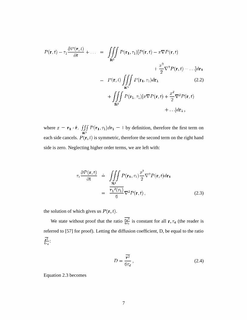
where � � �� . �� ! � �� # � � � �� by definition, therefore the first term on

each side cancels.! � � � �� is symmetric, therefore the second term on the right hand

side is zero. Neglecting higher order terms, we are left with:

# �� ! � � ��

�� ! � �� # � � � �� ! � � ��

� �� # � �� ! � � �� (2.3)

the solution of which gives us! � � � �� .

We state without proof that the ratio �� is constant for all � � # $ (the reader is

referred to [57] for proof). Letting the diffusion coefficient, D, be equal to the ratio

�� :

� � � �� # $ � (2.4)

Equation 2.3 becomes

7

� ! � � � �� ! � � � �� (2.5)

Equation 2.4 is called the Einstein equation, and Equation 2.5 is called the diffu-

sion equation, or heat equation. The quantity � � � � #%$ is a characteristic length

referred to in diffusion experiments as the Einstein length, the diffusion distance, or

the mixing length. #%$ is the time over which diffusion is observed, or the diffusion

time.!

is the diffusion displacement distribution, or conditional diffusion probability

density function (pdf): it has alternatively been called the diffusion propagator,

the diffusion Green’s function, and the van Hove self-correlation function. The

diffusion displacement distribution will be critical in our discussion of white matter

fibre tracking algorithms later in this thesis.

Diffusion can be observed as the diffusion of molecules or colloidal particles

in another medium, or simply the diffusion of molecules of one species in itself

(self-diffusion). It is self-diffusion that is important in diffusion MRI. Diffusion is

more rapid for smaller molecules, and self-diffusion coefficients of gases are higher

than those of liquids, which are higher than those of solids. Typical self-diffusion

coefficients of liquids are of the order 10 � mm � /s.

The diffusion equation can also be arrived at by considering the macroscopic

phenomenon of the change in concentration� � � � �� of a diffusing substance. Deriva-

tives with respect to time and space of� � � � �� and

! � � � �� are proportional. Fick’s

first law [59] relates the flux of the diffusing species to the change in concentration

via the diffusion coefficient:

� � � � � � � (2.6)

By combining Fick’s Law with the conservation of mass,

8

� �� (2.7)

we again derive the diffusion equation, which describes the change in concentration

with time:

� �� (2.8)

Equations 2.5 and 2.8 are identical except that the probability! � � � �� has been re-

placed by the concentration� � � � �� .

The root mean square (RMS) diffusion displacement during a diffusion MRI

experiment is of the order 10 � m, or roughly the diameter of a cell. The imaging

volume elements, or voxels, are typically of the order 10 mm . Hence, by mea-

suring the average diffusion displacement distribution!

in a voxel, we can infer

information about tissue structure on a scale far smaller than the voxel dimensions.

When the diffusion displacement distribution is anisotropic, the scalar�

is no

longer sufficient to describe the phenomenon. The Einstein equation is extended to

the anisotropic case by using a 3D covariant tensor, � , instead of the scalar�

:

� � � � �� #%$ (2.9)

� is symmetric for uncharged substances and is always positive definite and real

[182].

The isotropic and anisotropic descriptions of diffusion are both used to describe

diffusion in vivo, with applications to different normal and pathological situations

studied using diffusion MRI. In vivo, the diffusion of water is restricted by cell

9

membranes, myelin, organelles, and macromolecules. Technically, the water in the

intracellular compartment is said to be restricted and that in the extracellular com-

partment is said to be hindered. Water molecules moving with the same molecular

velocity as those in free solution have to travel longer distances to get from point A

to point B. For this reason, the diffusion coefficient of water measured in vivo is not

equal to that of pure water at the same temperature, and is often called the apparent

diffusion coefficient, or ADC. The diffusion coefficient and the ADC are related by

the tortuosity coefficient,�� :

ADCpure water ��

pure water��

� (2.10)

If the restrictive tissues have an anisotropic structure, the ADC will vary with di-

rection, and the voxel-averaged diffusion displacement distribution will be anisotropic.

Anisotropic diffusion is observable in muscle fibres and in nervous tissue fibres.

In nervous tissue, axonal membranes, neuronal filaments, and the myelin sheaths

surrounding the axons, contribute to anisotropy [19]. Diffusion is maximal in the

direction parallel to fibre bundles [99, 100], allowing the direction of the fibre bun-

dles to be inferred. An application of diffusion MRI that has generated significant

interest in recent years is the mapping of white matter fibre tracts in the central ner-

vous system, which involves first measuring the anisotropic diffusion displacement

distribution,! � � � �� , at each voxel.

It will be useful for later sections of this thesis to introduce the diffusion orien-

tation distribution function (ODF),( � � � , which is obtained from

! � � �� by inte-

grating out the radial information. � � � � � � � & � is a unit vector from the origin to

the surface of the sphere. We define

( � � � �( � � � �( �

� (2.11)

10

where

( � � � � ��

! � � �� #%$ � � � � (2.12)

( � � � contains the information in! � � � �� that is most important for fibre tracking

applications, that is, the changes in the pdf as the direction of interest changes.

Integration with respect to r is equivalent to projecting the pdf on the surface of

a sphere.( � � � preserves the variations in the pdf with respect to angle, but the

magnitude of diffusion and the variations in the pdf as r changes are removed.

Before we explore methods for reconstructing neuronal connections using the

diffusion pdf, we will first turn to the measurement of the ADC, the diffusion pdf,

and the diffusion ODF using diffusion nuclear magnetic resonance (NMR).

2.2 Diffusion NMR and MRI

2.2.1 Diffusion NMR

Well before the advent of magnetic resonance imaging, nuclear magnetic resonance

was used to measure properties of bulk samples of substances, without the addi-

tional information gained by spatial localization. Nuclear magnetic resonance was

discovered in 1946 by both Bloch (at Stanford) [22] and Purcell (at Harvard) [155].

In 1952, they were both awarded the Nobel prize in physics for their work.

NMR can measure many properties of different species, and the details will not

be treated here. The phenomenon pertains to all nuclei with non-zero angular mo-

mentum, i.e., those with an odd number of nucleons. The nucleus that is important

in fibre tracking with diffusion MRI is that of � H (the proton), and its host is the wa-

ter molecule. The particles that can produce an NMR signal will hereon be called

11

spins. The details of the physics of NMR will not be covered here, but the reader

may refer to texts and reviews such as [1, 162, 165, 166].

One of the physical properties measurable by NMR is the diffusion coefficient.

Prior to diffusion NMR, the diffusion displacement distribution was estimated by

using very similar, but differentiable, molecules, or measured using radioactive iso-

topes, neutron scattering, or laser scattering. The first NMR measurements of the

self-diffusion coefficient, performed in the early 1950s by Hahn [70], Carr, Pur-

cell [37], and others, were done using spin-echo NMR. The Bloch equation was

extended by Torrey in 1956 to include the effects of diffusion and flow [175]. An

analytic solution to the Bloch-Torrey equation for free diffusion was first given by

Douglass [55].

We will now introduce the diffusion sensitizing magnetic field gradient and de-

rive its effect on the NMR signal. We will first briefly describe the behaviour of

magnetic moments in the presence of an external magnetic field. When subjected

to a magnetic field B, nuclear magnetic moments � precess about the magnetic

field vector. The precessional frequency is inherent to the nucleus in question and

is given by the product of the magnetic field strength and a constant called the gyro-

magnetic ratio. The gyromagnetic ratio, , for � H is 42.58 MHz/T. The component

of a vector in the transverse plane (the plane perpendicular to the applied magnetic

field B�) in NMR is commonly described using a complex number, such that the

vector has a magnitude and a phase, and its precession can be described by the

factor � ��

� .

Diffusion weighting in NMR is accomplished by applying strong magnetic field

gradients that cause moving (diffusing) spins to dephase, while leaving stationary

spins unaffected. By dephasing, we mean that the individual spins in a population

acquire different phases because of the different magnetic fields they experience as

12

they diffuse in the presence of the magnetic field gradient. The result of dephasing is

that the magnitude of the net magnetization from all spins in the sample decreases.

We assume that the diffusing nuclei undergo free diffusion, i.e., that there are

no boundary conditions to be considered in the solution of the diffusion equation

(Equation 2.5). The solution of the diffusion equation is then a Gaussian distribu-

tion:

! � � � �� (2.13)

In many cases, the displacement distribution!

is measured for only one time

point, #%$ , so we will refer to the measured spatial displacement distribution as! � � � # $ � . Additionally, the displacement distribution measured for a bulk sample

will be the average displacement distribution of all the molecules therein. In this

case,! � � � � � � #%$ � means the volume-averaged probability that a spin originally at � �

displaces to position � in time # $ . These notations are often used interchangeably.

Consider a population of nuclei in which each undergoes a discrete random walk

of N steps, moving � � $ every � $ seconds. � is a vector on the unit sphere, and � $

is assumed to be constant. After step�, in the presence of a constant field gradient

G, a spin will experience a new field � �� $ � equal to the field it experienced

at time 0, � � � � �� , plus the net displacement vector multiplied by the diffusion

gradient � :

� � � � $ � � � � �� $�� (2.14)

Here, B is along�� and its magnitude varies in the direction of G.

The precessional frequency of the spin changes with each step. The total phase,&

, accumulated for the spin after N steps will be, after Haacke [68],

13

& � � �� #%$ � � � � # $ � � � � �� (2.15)

where is the gyromagnetic ratio. Substituting from Equation 2.14, we have

& � � � � $ � $ ��

�� (2.16)

Letting �� , we can reduce this double sum to a single sum as follows,

where the first line is simply a rearrangement of the sums in Equation 2.16:

& � � � � $ � $ ��

� �

� � � � $ � $ ��

��

� � � � $ � $ �� (2.17)

&is now seen to be a sum over a large number (N) of a random variable. Hence,

from the central limit theorem, the probability distribution of&

is Gaussian. Con-

sider now spins at the magnet isocentre r=0, such that the net magnetic field seen

by non-diffusing spins is always B� �� , with B

�the magnetic field strength with no

applied gradients. Because the diffusion pdf is symmetric,& � � at the magnet

isocentre. Hence, at this point, the probability density function for&

is

� & �� &�

� (2.18)

The net magnetization from all the spins in the sample will be attenuated because

of the phase dispersion. The integral over all spins of the Gaussian pdf for&

gives

rise to an exponential signal decay:

14

� � � ��

� � � & � � &

� �� (2.19)

where

is the signal intensity. Define �� . With each step� � ��

in a spin’s random walk, there is an incremental phase accumulation� & ��

� � �� . Hence,

&� �

� � �� (2.20)

where #%$ � � � $ . Equation 2.4 in one dimension gives us the mean square displace-

ment resolved along k:� � � � � � � � . Hence,

&��

� � ��

� ��

�� (2.21)

Let � � � � �� . Combining equations 2.19 and 2.21 gives us an expression for

the signal decay due to diffusion,

� �� (2.22)

We emphasize that this equation was arrived at by assuming the diffusion pdf to be

Gaussian, and that non-Gaussian diffusion would result in non-exponential signal

decay.

In the case of the constant gradient G, � � �� $ and therefore � � � � # $ � � .

The b value describes the amount of diffusion weighting in an MR sequence. In

15

GG

90 180oo echo

TE

δ

∆

Figure 2.1: Pulsed-gradient spin echo (PGSE) diffusion weighted sequence

practice, a diffusion imaging sequence will have a �� radio frequency (RF) pulse

applied at #%$ � � , so that T � � decay is eliminated and all non-diffusing spins have zero

phase at the echo time TE= # $ (i.e., k(t)=0 at TE because the effect of all gradients

after the �� pulse is to unwind the phase). Because the phase accumulation clock

is modified at #%$ � � , the b value for such a constant-gradient spin echo sequence

decreases to � � � � # $ � � � [97].

For imaging applications, it is easier to use the pulsed-gradient spin echo (PGSE)

method of diffusion encoding developed by Stejskal and Tanner in 1965 [169].

Here, two large, identical gradients of duration�

are applied on either side of the

�� pulse, with time�

between the start of the first and the start of the second (see

Figure 2.2.1). The b value achieved in this manner is � � � � � � � � � � � � � [97].

The effective diffusion time is� � � � � .

16

In the above derivation, we have assumed that the sample contained a freely

diffusing substance, i.e., that the diffusion displacement distribution! � � � �� was

an isotropic Gaussian function. In the case where the volume-averaged diffusion

pdf is non-Gaussian (e.g., when there are multiple diffusion compartments in slow

exchange, or restrictive barriers), the NMR signal will no longer be monoexponen-

tial. In 1968, Stejskal and Tanner solved the diffusion equation, predicted the NMR

signal decay, and verified their equations experimentally for the cases of planar dif-

fusion (a mica stack) and spherical restriction (yeast cells, apple tissue, and tobacco

pith) [172]. Note that in anisotropic systems, the value of�

measured by a diffu-

sion NMR experiment with a single gradient direction will be the projection of the

variances of the diffusion pdf on this direction [190].

It will be useful for later sections of this thesis to consider the exact form of the

diffusion weighted signal, regardless of the form of the diffusion pdf, in the case

where the PGSE diffusion sensitizing gradient duration�

goes to zero.

Let the vector q be a unit phase encoding step,

� � ��

� � � � (2.23)

where G is the diffusion sensitizing gradient in a diffusion weighted sequence. As�� , the phase accrual for a spin that moves from position r

�to r in time #%$ is

& � � � � � � � � � . For each voxel, the received signal S as a function of q is

� � � ��

�

��

��! � � � � ! � � � � � � # $ � � �� & � � � & � � � (2.24)

where ! is the proton density. This is the 3D inverse Fourier transform of the aver-

17

age probability density function,! � � � � � � # $ � , for diffusion in that voxel. This means

that the pdf can be calculated by acquiring images at a range of q values and per-

forming a 3D Fourier transform. For a Gaussian pdf!

, all terms after the quadratic

term in the cumulant expansion of! � � � # $ � will be zero [170]. Additionally, in the

small � limit, the higher order terms of the Fourier transform of! � � � # $ � will be

negligible [14], even if the underlying displacement distribution is non-Gaussian.

Hence, it is necessary to use a sufficiently high value of � in order to detect high

spatial frequencies in the diffusion pdf. This will be discussed in more detail in

Section 2.2.6.

2.2.2 Diffusion weighted imaging

In the 1970s, Lauterbur [93] and Mansfield [105] made the discoveries that would

lead the way to the development of modern magnetic resonance imaging. In 2003,

they were awarded the Nobel prize in physiology or medicine for this work. The

crucial step between previous NMR experiments and MRI was the development of

a method to map properties measurable by NMR at different spatial locations, i.e.,

to form an image. The details of MRI acquisition and image calculation will not

be presented here, however, the reader is referred to texts on the subject [26,27,68,

106, 119, 124, 144].

It was not until 1985 that diffusion NMR and imaging techniques were com-

bined. Diffusion MRI added a new contrast mechanism to the traditional T � and T �relaxation times: it was now possible to visualize clinical conditions that changed

the properties of molecular diffusion of water. Diffusion MRI was first performed

by Taylor and Bushell [173], who used a hen’s egg as a phantom in a small bore

magnet. Diffusion imaging was performed for the first time on a whole body scan-

ner by Le Bihan [96]. A diffusion weighted image (DWI) is one where the acqui-

18

sition sequence had one or more diffusion sensitizing gradients: voxels with high

diffusion in the direction of the gradient will have a greater signal attenuation than

those with low diffusion. For example, in ischemia, which was one of the first appli-

cations of diffusion MRI [92] and for which diffusion imaging is now a standard, the

magnitude of diffusion is decreased. This occurs because injury following ischemia

is characterized by a depletion of high-energy phospho-metabolites and a rapid ele-

vation of inorganic phosphate and lactate. Impairment of energy metabolism causes

failure of the cell membrane’s sodium-potassium pump, which regulates the intra-

and extra-cellular Na � , K � , and � ��

concentrations. The cell membrane becomes

impermeable, and the cell swells with water. The ADC is thus decreased because

the movement of � ��

between cells is slowed down due to this added hindrance.

Stroke can also be imaged with�� weighted MRI, however, diffusion contrast is

evident well before�� contrast [112].

Sample images with different diffusion weightings are shown in Figure 2.2. Fig-

ure 2.2a has no diffusion weighting, i.e., b=0 s/mm � . Figure 2.2b was acquired with

b=1300 s/mm � . The window level has been changed to show the images clearly: the

b=0 s/mm � image has a significantly higher signal to noise ratio (SNR), as expected.

The ventricles have far more signal attenuation than do grey and white matter, due

to the lack of restrictive barriers (cell membranes, organelles, macromolecules) in

CSF. The diffusion contrast in tissue that has anisotropic diffusion properties is de-

pendent on the direction of the diffusion encoding gradient, hence, we can measure

anisotropic diffusion displacement distributions by acquiring multiple images with

gradients in different directions. It is possible to achieve a directionally invariant

diffusion weighted image by applying diffusion encoding gradients sequentially in

three orthogonal directions.

19

a b

Figure 2.2: Diffusion weighted imaging. (a) Image with no diffusion weighting(b � 0 s/mm � ). (b) Diffusion weighted image with b=1300 s/mm � . The windowlevel has been changed to show the images clearly: the b=0 s/mm � image has asignificantly higher signal to noise ratio (SNR), as expected. The signal strength(arbitrary units) is shown on the color bars.

2.2.3 Scalar parameters from diffusion imaging: apparent dif-

fusion coefficient (ADC) and anisotropy index (AI)

Because of the long echo time (TE) necessary to achieve diffusion weighting, dif-

fusion weighted scans are necessarily T � weighted as well. This effect is often

referred to as “T � shine-through”. Given multiple diffusion weighted images, it is

possible to calculate quantitative scalar parameters that describe the diffusion only,

eliminating contrast due to T � differences. From Equation 2.22, the ADC can be

calculated in each voxel using linear regression on the log-transformed images:

�� ADC � (2.25)

We have discussed above the anisotropic nature of diffusion in tissue, which

20

causes the magnitude of the diffusion weighted signal, � �� , to vary in any anisotropic

voxel as the direction of the diffusion encoding gradient varies. Hence, if we were

to measure separate ADCs (ADC � , ADC � , ADC � ) with gradients in the � , � , and �

directions, we should be able to describe the degree of anisotropy in the tissue. In

brain white matter, the ADC in the direction parallel to the fibre bundles has been

found to be as high as 10 times that perpendicular to the fibre bundles [151].

The first anisotropy index (AI) measured in a biological sample was defined

by Cleveland et al. in the context of diffusion NMR [47]. The middle portion of

the tibialis anterior muscle of mature male rats was scanned in a spectrometer and

rotated so as to measure the ADC at 0�, 45

�, and 90

�. The ratio ADC � /ADC � �

was measured to be 1.39.

The first in vivo anisotropy index measurement was performed by Moseley et

al. [121] in cat brain. The AI defined was the ratio ADC � /ADC � . This and other

anisotropy indices defined using three ADCs have the confounding issue that they

are rotationally variant: in the next section, we shall describe methods of measuring

rotationally invariant measures of anisotropy.

2.2.4 Diffusion tensor imaging (DTI)

In Section 2.1, we defined the diffusion tensor, D, which appears in the description

of anisotropic diffusion (Equation 2.9). An anisotropic solution of the diffusion

equation (Equation 2.5) is a 3D, anisotropic Gaussian distribution:

! � � � � � � # $ � � �� # $ � � �� #%$ � (2.26)

In 1994, Basser et al. recognized that the diffusion pdf for the restricted and

hindered diffusion in tissue could be modeled as such a Gaussian distribution [15].

21

Restricted diffusion is never truly Gaussian: there are deviations from the Gaussian

model in both the radial and angular dimensions, however, in many cases, such as

that of single subvoxel white matter fibre directions, the Gaussian model is adequate

to describe the voxel-averaged pdf. Measurement of a diffusion tensor at each voxel

in the MR volume was termed diffusion tensor imaging (DTI).

The assumption of a single-Gaussian displacement distribution is a low spatial

frequency approximation of the diffusion pdf. With this assumption, it is possible

to estimate the diffusion pdf using only seven data points (nonzero b values in six

directions and one other measurement, generally with b � 0), although in practice

more measurements are usually made. In DTI, the single b value is replaced by a b

matrix, b, and the tensor elements are computed by solving the following:

� ��

�� (2.27)

The diffusion tensor D is symmetric, positive definite, and real: these constraints

can be used in its estimation [18,179]. Its eigenvalues are real and positive, and the

eigenvectors are real and orthogonal. The eigenvector corresponding to the largest

eigenvalue (often called the principal eigenvector, e � ) is aligned along the maximum

of the Gaussian displacement distribution and is used as a measure of the fibre di-

rection in voxels in which oriented fibre structure exists. The trace of the diffusion

tensor gives a measure of the mean diffusivity. In fact, because the trace is pre-

served under rotation, the trace is equal to the sum ADC � +ADC � +ADC � measured

by applying three orthogonal gradients and computing the ADCs without comput-

ing the tensor. The eigenvalues of the tensor can be used to calculate rotationally

invariant anisotropy indices, and many such indices have been proposed. Those

which require sorting of the eigenvalues overestimate anisotropy in the presence of

noise, which has lead to the definition of several indices that are not susceptible to

22

this sorting bias. The volume fraction (VF) has a nice intuitive description: it is

equal to one minus the ratio of the volume of an ellipsoid whose semi-major and

semi-minor axes are the three eigenvalues of D, divided by the volume of a sphere

whose radius is the mean diffusivity. If there is no anisotropy, these volumes are

the same, and the volume fraction is equal to zero. The maximal value of this index

is 1:

��

� (2.28)

Another rotationally invariant AI, again with a range of 0-1, with 0 representing

isotropic diffusion, is the fractional anisotropy [151]:

��

� � � � � � � � � � � � ��

� (2.29)

Other similar AIs, which are essentially second moments of the tensor, include

the relative anisotropy (RA):

��

� � � � �� (2.30)

and A � [50]:

��

�" � � �� (2.31)

23

Here,� � trace � � � � � and " � � � � � � trace � � � � �� . The original definition

of the RA was not scaled to lie between 0 and 1, but it now often is. These AIs

provide slightly different contrast. The FA has higher noise immunity than does the

RA [72].

The calculation of the tensor is a statistical procedure and estimates of D can

therefore be accompanied by measures of uncertainty and goodness of fit, such as

� � statistics [131, 163]. Given sufficient data, bootstrap statistical methods can be

used to estimate confidence intervals or a marginal posterior distribution for the

direction of the principal eigenvector [20, 82].

Figures 2.3 and 2.4 show examples of images obtained from DTI of the human

brain. The base images were acquired using a Siemens 1.5T Sonata MR scan-

ner (Siemens Medical Systems, Erlangen, Germany), with b=0 s/mm � and 1300

s/mm � , TR=8s, TE=110ms and 2.5 mm isotropic voxels. Figures 2.3a-c are exam-

ples of diffusion weighted images: note the different contrast when the diffusion

encoding gradients are applied parallel and perpendicular to fibre structure. Figure

2.3d shows the calculated FA map, and Figure 2.3e the trace of the diffusion ten-

sor. Note that the FA is high in the major fibre tracts and low in regions of more

isotropic diffusion. The trace is high in CSF and relatively constant in all other re-

gions of the brain. This constancy in grey and white matter is because the average

degree of restriction is the same in both types of tissue: the restrictive barriers are

simply more organized in white matter, such that diffusion is higher than average

parallel to fibres and lower than average perpendicular to fibres. Figure 2.3f is a red-

green-blue (RGB) plot indicating the direction of the principal eigenvector scaled

by the anisotropy index. This visualization approach was introduced by Pajevic and

Pierpaoli [130], and is a popular method of showing the inferred fibre directions in

DTI. Here, red represents the component of the principal eigenvector of the diffu-

24

a b c

d e f

Figure 2.3: Diffusion tensor imaging: (a-c) Diffusion weighted images with diffu-sion encoding gradients in different directions: note the difference in contrast as thediffusion encoding direction changes. (d) Fractional anisotropy (FA). (e) Trace im-age. (f) RGB map showing principal eigenvector direction and FA. In (a-c), bright-ness is proportional to signal strength, in (d) and (f), brightness is proportional tothe FA, and in (e), brightness is proportional to the trace.

sion tensor in the left-right direction, green the component in the anterior-posterior

direction, and blue the component in the head-foot direction. Figure 2.4 shows the

principal eigenvector directions projected on the transverse plane overlaid on the

scalar FA image.

The diffusion tensor model provides a very useful tool for investigating anisotropic

tissue structure, however, there are a number of cases it does not handle well. These

include subvoxel fibre crossing, curvature, branching, splay, and highly restricted

diffusion. The single tensor model also cannot describe subvoxel heterogeneity in

25

Figure 2.4: Diffusion tensor imaging: projection of principal eigenvector on thetransverse plane, overlaid on FA map.

26

the radial direction, i.e., fast and slow diffusion compartments.

2.2.5 Restoration of diffusion tensor data

The calculated diffusion tensor field can be discontinuous and noisy. Methods for

smoothing the diffusion weighted images, the diffusion tensor field, or the principal

eigenvector field have been explored. Regularization algorithms use information

from neighbouring voxels and assumptions of stiffness or curvature to restore noisy

or discontinuous data. One of the original approaches was that of Aldroubi et al.,

who published a method for calculating a Lipschitz continuous tensor field from the

discrete tensor data [4].

When smoothing diffusion data, we wish to propagate information along the

direction of fibre tracts, that is, it is sensible for the smoothing kernel to resemble

the diffusion tensor itself, with a maximum along the fibre direction. This leads

to preservation of anisotropy and propagation of information along directions in

which we have high confidence in there being oriented fibre structure. Anisotropic

diffusion smoothing techniques were pioneered by Perona and Malik [147] for edge

preservation when smoothing scalar images, and are well developed in the computer

vision literature: applications include the enhancement of flow-like patterns in im-

ages [198, 199], and optical flow calculations [9]. They fall into a larger category

of partial differential equation (PDE) based smoothing schemes [198]. Many non-

linear smoothing techniques have been proposed for restoration of diffusion tensor

data. For example, Parker et al. have used the nonlinear smoothing techniques of

Perona and Malik to smooth noisy diffusion weighted images prior to calculation

of the diffusion tensor, and have shown that this approach provides superior results

to smoothing the calculated FA maps [137].

A number of the nonlinear smoothing approaches employ variational principles

27

that lead to PDEs, while others define PDEs directly. In the variational approaches,

as in other regularization frameworks, the principle is to perform smoothing while

maintaining fidelity to the data, hence, a regularization term and a data term ap-

pear in the variational formulation, along with other constraints such as positive-

definiteness. Edges, or abrupt changes in the tensor or vector orientation, are pre-

served. The variational approach consists of defining an energy or cost functional

that is to be minimized, and solving the PDEs that result from minimizing that

functional. Coulon et al. extend the total variation (TV) norm framework of Chan

and Shen [42] to regularize the principal eigenvector field, and subsequently use

an anisotropic diffusion process to regularize the three eigenvalues [52]. Vemuri

et al. [187, 195] also use the TV norm framework, however, smoothing is done

on the original diffusion weighted images. A selective term that is a function of

the anisotropy index is used to preserve anisotropy. In more recent work by this

group, simultaneous estimation and smoothing of the diffusion tensor field is per-

formed [194]. Tschumperle, Chefd’hotel, Deriche, et al. have used nonlinear PDEs

to restore the full tensor field [43, 179]. Other nonlinear filtering techniques in-

clude the work of Hahn et al. for restoring the full tensor field [71] and the work

of Westin and Knutsson, who use a nonlinear filtering technique called normalized

convolution [201] to regularize the full tensor field. Many of these approaches reg-

ularize both the orientation (angular) information, or that given by the eigenvectors

of the diffusion tensor, and the diffusivity (magnitude) information, or that given

by the eigenvalues of the diffusion tensor. These regularization processes are sepa-

rated [43, 52, 179, 201].

We will briefly describe one of the earliest variational approaches [52] for reg-

ularizing diffusion tensor data, as these approaches are becoming increasingly pop-

ular. We wish to regularize the principal eigenvector orientations, which lie on the

28

unit sphere� . Let � �� be the total variation energy, which we wish to minimize in

order to obtain the regularized direction map. After [42],

� � � � � � � � � ��

��

�� (2.32)

where

�� (2.33)

Here,�

and�

are indices for voxels in the discretized image domain� �

and � �

is a neighbourhood of voxel�.�

represents the principal eigenvector field, with� � � �

the original vector field and� � the principal eigenvector direction in voxel

�.

��is a measure that tends locally to the metric on

� : in the implementation of

Coulon et al., the Euclidian distance is used. The first term in Equation 2.32 is

a regularization term: it is low if the principal eigenvector directions are locally

coherent. The second term is a data term: it requires the regularized vector field

to be close to the original field.�

controls the extent to which the regularization is

data-driven. The Euler-Langrange equations associated with Equation 2.32 lead to

the following differential equation:

� � ��

� � � �� (2.34)

where

� � � � � � ��

�� (2.35)

and� � � is the projection on the plane tangent to the unit sphere at

� � . The projection

means that the eigenvector directions can only change in orientation, i.e., they are

constrained to have unit length.� �� is equal to

� � if� � � � � � and is equal to � � �

otherwise, such that�

and � � are equivalent, as is the case for principal eigenvector

29

directions. Coulon et al. modify the weighting factor in Equation 2.35 to be

� � � � � � � � � � � � �� (2.36)

where FA is the fractional anisotropy and � is an adjustable control parameter that

is set in this implementation to 2. This weighting has the result that a neighbour-

ing voxel will not influence another voxel strongly if it has (a) a very different

vector orientation, for example, at boundaries between different fibre tracts or (b)

low anisotropy, in which case its principal eigenvector direction is not particularly

meaningful. This regularization algorithm therefore produces a principal eigenvec-

tor field that is locally smooth while preserving “edges” between fibre populations

and isotropic tissue.

Other approaches to the regularization problem include the Bayesian framework

pioneered by Poupon et al. [152] for regularization of the principal eigenvector

field. Martin-Fernandez et al. have also used a Bayesian framework for regularizing

the full diffusion tensor [107]. Further developments for smoothing the full tensor

field include the work of Pajevic et al. [129] on computing a continuous tensor field

by repeatedly performing B-spline transforms on the diffusion tensor data.

In addition to smoothing the diffusion tensor and/or principal eigenvector field,

regularization can be used to infer multiple intravoxel fibre directions based on

neighbouring information. As mentioned in Section 2.2.4, the single-Gaussian

model may not be a suitable model in many voxels. Given a diffusion tensor field,

a multi-tensor or multi-vector field can be reconstructed using information from

neighbouring voxels and regularization constraints. One technique for doing so is

the spin-glass framework, derived from a technique in statistical physics, developed

by Cointepas et. al. [48] for inferring multiple fibre directions in cases of partial

volume averaging. Additionally, from a diffusion tensor field, one can inversely

30

solve for the coefficients of a predefined multi-tensor basis field in order to restore

complex intravoxel information [157]. This approach uses propagation of infor-

mation from high anisotropy regions to lower anisotropy regions, and employs a

Bayesian regularization framework.

2.2.6 High angular resolution diffusion imaging

We have described regularization techniques that attempt to solve for multiple fibre

directions in a given voxel, based on information from the voxel’s neighbourhood.

These methods are potentially powerful for resolving multiple intravoxel fibre di-

rections, but may be problematic in cases where different fibre populations are prox-

imal, in large regions of crossing, or in cases of high curvature. In the techniques

described in [48,157], the tensor is first calculated from the base diffusion weighted

images, and then an inverse problem is formulated to infer multiple maxima in the

diffusion pdf. It could possibly be more suitable to calculate the diffusion pdf at

high angular resolution directly from the data, without ever invoking the single-

Gaussian assumption. This section addresses the topic of high angular resolution

diffusion (HARD) imaging. The goal of HARD imaging is to capture information

about multiple intravoxel fibre directions.

We note that the diffusion pdf can have non-Gaussian characteristics in both

the radial and angular dimensions: we will concentrate on the latter, as it has more

obvious implications for fibre tracking. There is a growing body of literature on

multi-tensor and related approaches for looking at multiple diffusion magnitude

compartments, e.g. [46].

31

High angular resolution ADC measurement

Measurement of the ADC at high angular resolution in order to obtain a two-

dimensional surface, or ADC profile, can be expected to give us information about

intravoxel heterogeneity of fibre directions. This method does not, however, give

us the directions of the maxima of the diffusion pdf. In fact, because the ADC is

a projection of the variances of the pdf (see Section 2.2), the maxima of the ADC

profile are not directly related to the maxima of the diffusion pdf at all. This has

been shown in phantom [189] and in vivo [184], as well as analytically (using a

cylindrical diffusion model) [189]. Hence, the applicability of high angular reso-

lution ADC measurements to fibre tracking is not clear: further post-processing of

these measurements in necessary.

The high angular resolution ADC profile is useful for identifying cases where

multiple fibre directions are present [7]. The profile can be characterized using

spherical harmonics and similar approaches [7, 60, 77, 128, 134, 189, 208].

In general, even if diffusion weighted measurements are made at high angular

resolution, non-Gaussian diffusion can only be observed if the b-values used are

sufficiently high to resolve differences in the diffusion weighted signal over small

changes in the orientation of the diffusion weighting gradient, � . If low b-values

are used, the ADC profile will be indistinguishable from that of Gaussian diffu-

sion. Zhan et al. [208] and Von dem Hagen et al. [189] have shown the increasing

structure in the ADC profile as the b-value increases.

High angular resolution diffusion pdf measurement

In the previous section, we stated that the ADC profile can tell us when there may be

multiple fibre directions in a single voxel, but it cannot tell us what those directions

are. The diffusion pdf can, because it is maximal in the direction parallel to the

32

axons of the neurons that comprise fibre bundles [100,101,180]. In this section, we

will explore how to go from diffusion weighted measurements in many directions

to a high angular resolution estimate of the diffusion pdf or ODF. In some cases,

this can be a significant improvement over the ODF estimated with the diffusion

tensor model (see Figure 2.5).

A logical extension of the single-Gaussian model of diffusion is to allow for

multiple Gaussian compartments. In its most general sense, this method allows

for multi-Gaussian behaviour in both the radial and angular dimensions. Multi-

tensor approaches for the purpose of achieving higher angular resolution have been

suggested by Alexander et al. [5] and pursued by others [23, 184]. Many of these

make assumptions about the magnitudes and ratios of the eigenvalues [5] and have

been found to be unstable when the number of compartments is greater than two

[184].

An alternative to the multi-tensor approach is model-free reconstruction of the

diffusion pdf. In Section 2.2.1, we have described the q-space formalism for a

general diffusion pdf. Inverting Equation 2.24, we have:

! � � � � � � � � � � � �� (2.37)

In practice, the phase of S(q) is modulated not only because of diffusion, but

because of bulk motion and field inhomogeneities. However, we know that the pdf

is real, therefore S(q) is Hermetian, and the pdf is symmetric, therefore S(q) is real.

We can retrieve the pdf by taking the 3D Fourier transform of �S(q) � , and only half

of q-space need be acquired by symmetry.

The resolution of the computed pdf will be the inverse of the maximum q value

achieved. Increasing the duration of the diffusion encoding gradients (�) increases

the echo time, which in turn decreases SNR. With the value of�

limited to rea-

33

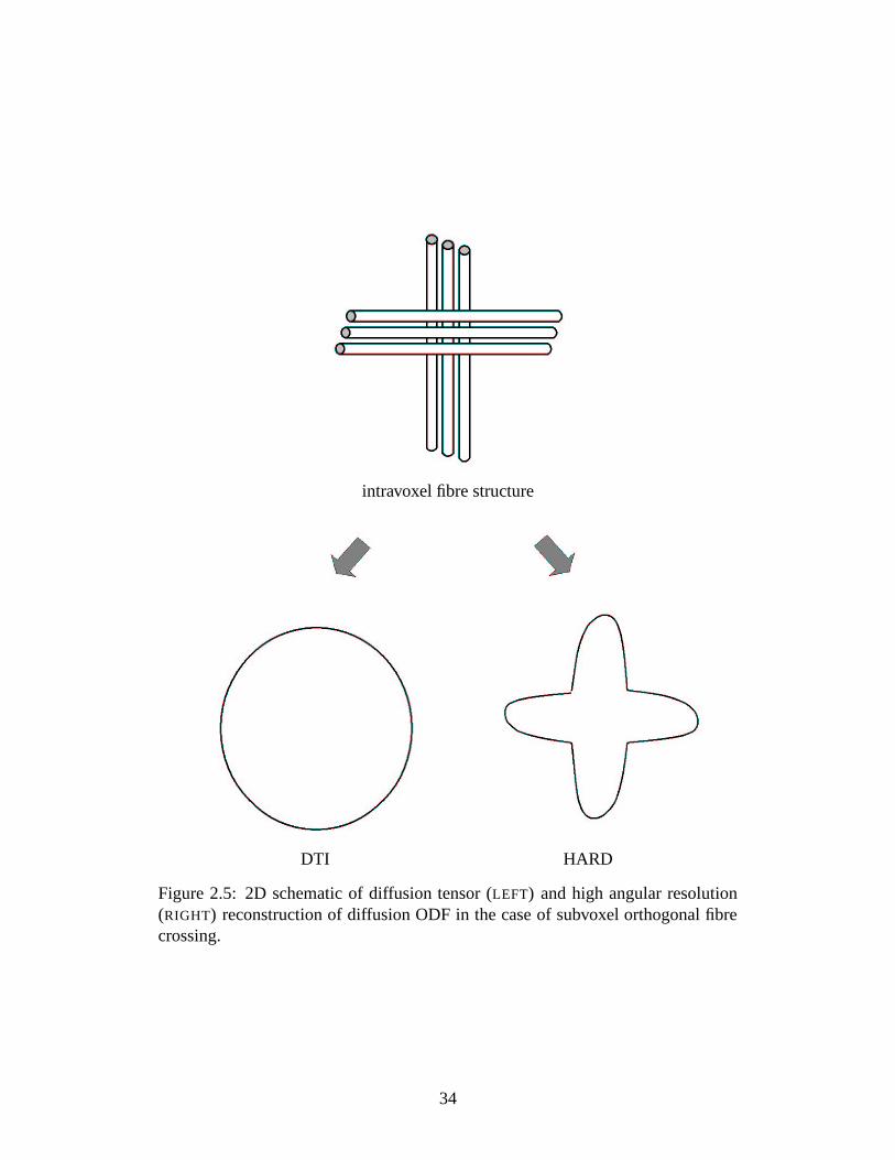
intravoxel fibre structure

DTI HARD

Figure 2.5: 2D schematic of diffusion tensor (LEFT) and high angular resolution(RIGHT) reconstruction of diffusion ODF in the case of subvoxel orthogonal fibrecrossing.

34

sonably small values, the factor limiting the maximal value of q is the maximum

gradient strength possible. Modern MR scanners with large gradient strengths (e.g.,

40 mT/m) allow pdf resolution on the order of 1-10 � m, which is the expected RMS

displacement of water molecules in tissue. The field of view of the computed pdf is

inversely proportional to the density of q values obtained. Q-space pdf reconstruc-

tion requires very high b-values because the signal must be very low at the edge of

the measured portion of q-space in order to avoid Gibb’s ringing artifacts. Hence,

q-space imaging is technically demanding.

Q-space imaging has been performed by several groups. While the methodology

can potentially enable measurement of high spatial frequencies in both the radial

and angular dimensions, in the earlier work the Fourier transform was done in only

the radial dimension (in 1D) [12, 87, 88]. With sufficient data, the full 3D Fourier

inversion can be performed: this technique for measuring a high-radial and high-

angular pdf has been termed diffusion spectrum imaging (DSI) [197]. There is

debate as to whether DSI on clinical MR scanners is truly q-space reconstruction,

because current technology requires the value of�

to be long, while the q-space

formalism requires�

to be infinitesimally short. For the purpose of achieving high

angular resolution, this is of little consequence, as the effect of the finite gradient

duration�

is simply a convolution over different diffusion times [113].

In the tissue of the nervous system, we expect to see highly restricted (non-

Gaussian) diffusion compartments and approximately Gaussian, hindered compart-

ments. Assaf et al. have developed a pdf reconstruction method that accounts for

these two compartments via a combined q-space and diffusion tensor model [11].

The model allows for multiple restricted compartments, i.e., multiple fibre direc-

tions.

For the purpose of fibre tracking, we want to measure the diffusion orientation

35

distribution function,( � � � (see Section 2.1).

( � � � can be obtained from the dif-

fusion pdf measured with q-space, diffusion tensor, combined q-space and tensor,

or multi-tensor approaches. The q-space and multi-tensor methods give more in-

formation, especially in cases of partial volume averaging of fibre directions, than

does the single-tensor approach. However, they require more measurements and/or

more postprocessing. In the case of multi-tensor approaches, the additional infor-

mation is limited by the model chosen. Measurement of more than two directions

has been shown to be unstable [184]. If only the angular information is desired, it

is superfluous to estimate the entire 3D diffusion pdf and to integrate out the radial

information afterward.

Recently, Tuch et al. have developed a method for estimating the diffusion

ODF directly from measurements on a single sphere in q-space [181]. This method,

called q-ball imaging (QBI), is extremely powerful, as it requires far less data to es-

timate an ODF at a given angular resolution than does q-space imaging, which in-

volves estimation of the full pdf in the radial direction before the ODF can be calcu-

lated. Additionally, it does not require the extremely high b-values (e.g., b=20 000

s/mm � [197]) necessary to avoid Gibb’s ringing in the Fourier-transformed diffu-

sion pdf. High b-values (e.g., b=4000 s/mm � [182]) are still required, however, to

ensure that higher order variations in the angular direction are detectable. We will

derive the relationship between the diffusion-weighted measurements on a sphere

in q-space and the diffusion ODF, as the QBI reconstruction method will be central

to later sections of this thesis.

Given N measurements on the surface of a sphere in q-space, we want to mea-

sure the diffusion orientation distribution function,( � � � , given by Equation 2.11.

( � � � can equivalently be calculated by first projecting the pdf on the plane perpen-

dicular to � , and subsequently taking the value at the origin:

36

( � � � �� ! � ��

�� ! � � � � � �� (2.38)

where we have written!

in cylindrical coordinates with the � axis along u. We

will now show that( � � � can be approximated by the Funk-Radon transform of

the diffusion weighted measurements � � � . Again in cylindrical coordinates, the

Funk-Radon transform�� of

� � � is given by [63, 181]:

��

� ��

� �� (2.39)

This represents the integral around a great circle of radius � � in the plane perpen-

dicular to � .� � � ��

� � �� , with��

the 0 ��

order Bessel function.

By the central slice theorem [156], Equation 2.37 implies that� � ��

� ! � � � � � �� . Hence, Parseval’s Theorem (energy preservation) [156] gives:

��

� �� ! � � � � � � � �� (2.40)

Comparing to Equation 2.38, we can see that

( � � �� (2.41)

to the extent that the Bessel function� �

resembles a delta function. In other words,

the Funk-Radon transform of the diffusion-weighted signal gives a blurred ODF,

with the amount of blurring determined by the width of� � � � � � � � � . The higher the

37

value of � � , the sharper the approximated ODF will be.

Tuch’s implementation of the QBI technique requires 492 directions and was

done for only two noncontiguous slices of the brain: while promising, it and q-space

methods require a very long acquisition time for the full brain, which is necessary

for many fibre tracking applications.

Alexander et al. also have developed a model-independent method of estimat-

ing the diffusion ODF [8]. The technique, called persistent angular structure MRI

(PAS-MRI), is based on the principle of maximum entropy. Results have been

shown using lower b-values and fewer diffusion encoding directions than QBI.

However, processing times are long for this reconstruction method.

One argument in favour of the tensor model is that it requires fewer measure-

ments to be made. However, standard diffusion imaging techniques make it pos-

sible to make many more measurements in a clinically feasible amount of time:

the use of 60 measurements has been recommended [81] and is often used for the

purpose of signal averaging. Given that N measurements will be made, it has been

shown [83,133] that it is better to make different measurements (i.e., apply diffusion

weighting gradients in different directions) than to average the same measurements.

Hence, the optimal strategy for measuring the tensor may not be very different from

that for measuring a high angular resolution ODF, with the exception of the higher

b values which facilitate HARD imaging.

2.3 Fibre tracking

As stated in Chapter 1, the digital reconstruction of fibre tracts in the human central

nervous system is a problem of considerable interest, with widespread applications

in basic neuroanatomical research and neurological disease. The 3D digital curves

arrived at using tractography provide a powerful visualization tool for viewing dif-

38

fusion data: although it is often easy for the human eye to infer connections when

presented with a two dimensional array of diffusion ODFs and/or their maxima, it

is extremely difficult to make sense of a three dimensional array of such data. Thus,

plotting curves in 3D makes visualization of potential connections much easier for

the observer. Tractography makes decisions for the user as to which connections

are and are not present, hence it is clear that the fibre tracking algorithm must be

robust if any conclusions are to be made from it. The field of MR fibre tractography

is rapidly developing. This section presents a summary of the body of literature on

the subject, much of which was published in parallel with the research that will be

described in Chapters 3-6.

We note here that unlike the connectivity inferred from tracer studies, the con-

nectivity inferred from diffusion MRI data is not at a cellular level. Because the

diffusion pdf is a voxel-averaged measure, the best resolution a fibre tracking algo-

rithm can have is on the level of fibre bundles. We can hope to determine whether a

given imaging voxel is connected to another, but subvoxel resolution is not possible.

Ultimately, the level on which connectivity can be assessed will depend on imaging

resolution and specifics of the tractography algorithm used.

2.3.1 Methods for reconstructing connections

The simplest estimate of the fibre orientation in any one voxel is the principal eigen-

vector of the diffusion tensor, � � . Fibre tracking algorithms that propagate along the

direction of the maximum of the diffusion pdf are collectively called principal dif-

fusion direction (PDD) methods. In its simplest form, tracking starts at the centre

of a seed voxel, and the next point will be the centre of the voxel pointed to by

the principal eigenvector � � at that voxel. Such algorithms that connect vectors in

a 3D vector field to create curves are called streamline algorithms, in analogy to

39

standard methods for finding paths through vector fields. Such methods have been

developed, for example, in the field of fluid mechanics [44].

Tracking from voxel centre to voxel centre can easily lead to deviations from an

actual fibre tract, as imposing a grid on what is in fact a continuous pathway leads to

discretization errors. Mori et al. have developed an algorithm called Fibre Assign-

ment with Continuous Tracking (FACT) [115] which addresses the discretization

issue. From each seed point, the reconstructed tract follows the direction of that

voxel’s � � until it enters another voxel, at which point the direction of propagation

immediately changes to that of � � of the new voxel. The data can be supersampled

prior to tracking as much as is practical in terms of computation time. In FACT

and in most other fibre tracking algorithms, stopping criteria are used to determine

where a reconstructed pathway should end. These typically consist of curvature

constraints and limits on the anisotropy index. Curvature constraints of 45�

[192]

and anisotropy thresholds of FA � 0.2-0.4 [115] have been used with FACT tracking.

These are quite strict, and we will see later that there are benefits to using less strict

thresholds, which facilitate tracking through regions of lower anisotropy (e.g., the

thalamus) or higher curvature (e.g., subcortical fibres).

A slightly different approach from that of continuous tracking is the constant

step size (CSS) approach, in which tracking proceeds from a seed point with steps of

constant length in the direction of � � , and after each step, the principal eigenvector

is recalculated from interpolated diffusion data [51]. Step sizes of one half the

original voxel dimension have been shown to be optimal in this approach [103],

with little gain from using smaller step sizes.

More formal streamline methods include the use of numerical integration to

obtain a parametrized curve � � � � in 3D space [16]. The tangent to this curve � � � � is

given by � � � � � � � � � � � � � , so that

40

� � � � �� (2.42)

Equation 2.42 is called the Frenet equation describing the evolution of � � � � . It

can be solved numerically by Euler’s method or the Runge-Kutta method (RK4).

A continuous representation of the diffusion tensor field is first calculated using

fast filtering algorithms [4], providing a continuous � � vector field with which to

solve equation 2.42. The D field allows higher order derivatives of � � to be taken,

making the use of the Runge-Kutta algorithm possible. Higher order derivatives

of � � � � are also used to calculate the curvature and torsion of the tract. This fibre

tracking algorithm uses four stopping criteria: (1) the boundary of the imaging

volume is reached; (2) the anisotropy index drops below a given threshold; (3) the

radius of curvature is smaller than approximately two voxels; (4) the tract reaches a

region where an eigenvector other than � � � � � � � � is more collinear with � � � � than is

� � � � � � �� . Other integral curve approaches include that of Vemuri et. al [187, 195],

who use a variational approach.

Other streamline PDD methods include diffusion tensor tracking (DTT) [102],

linear state space models [66], and ‘EZ’ tracing [174]. There has also been interest

in classifying or bundling regions of white matter based on the principal eigenvector

direction [54, 62, 84, 171].

PDD fibre tracking methods can be confounded by partial volume averaging of

fibre directions and can be particularly susceptible to noise. In the case where two

fibres cross in one voxel, the maximum of the single diffusion tensor may not lie

along the direction of either. The ODF defined using the tensor will be planar, and

small amounts of noise can cause the maximum to vary widely in this plane. This

has led investigators to consider using the full tensor, as in the method of tensor

41

deflection developed by Lazar et al. [95], or the multiple maxima derived from

regularization techniques [48], multi-tensor reconstructions [23], or DSI [182], to

propagate streamlines. These methods can significantly improve upon the results

of PDD streamline methods, however, it is desirable in many cases to quantify the

uncertainty that exists in the fibre tracking procedure. This is the topic of the next

section.

2.3.2 Likelihood of connection and probabilistic fibre tracking

Traditional streamline fibre tracking methods lack a statistical framework for in-

terpreting fibre tracking results. Approaches that attempt to assign a quantitative

index of connectivity can be divided into deterministic and stochastic tracking ap-

proaches, and give as output both tracts as 3D curves and a scalar measure of the

probability or likelihood that point A is connected to point B. The first such ap-

proach was proposed by Parker et al. [139, 142, 143], and used the principal eigen-

vector to drive a deterministic flow which yielded a quantitative index of connec-

tivity. Following this work, several flow-based approaches using the full diffusion

tensor were proposed [17, 31, 125, 177]. A Lagrangian approach using an arbitrary

diffusion ODF was also implemented [182]. The algorithm described in Chapter 5

of this thesis falls into this category, with a flow-based approach designed to use an

arbitrary estimate of the fibre orientation likelihood distribution.

Monte Carlo approaches to streamlines using the full diffusion tensor have been

implemented by Koch et al. [90], Hagmann et al. [69], Bjornemo et al. [21], and

Parker et al. [141]. Parker et al. have further applied the method to one- or two-

tensor fields depending on the adequacy of the single-tensor fit [140]. The multi-

tensor field obtained by Ramirez-Manzanares et al. using regularization has been

used to drive a stochastic tracking scheme [157], while the marginal posterior dis-

42

tribution for the principal eigenvector direction has been used by Behrens et al. [20]

for stochastic fibre tracking. Tuch et al. have implemented a stochastic simulated

annealing algorithm that can be used with DSI data [182].

Many of these probabilistic methods use stopping criteria that are far less strict

than those used in traditional streamline methods. For example, Parker et al. use

no anisotropy index constraint [138], while Behrens et al. use an 80�

curvature

constraint [20]. While use of such constraints with traditional streamline algorithms

may result in a mass of relatively uninterpretable tracts, the addition of an index of

likelihood of connection helps determine which tracts are valid connections. Hence,

probabilistic and other related approaches are better suited for tracking through

regions of low anisotropy, such as deep grey matter structures through which tracts

do pass, and near the highly convoluted cortex.

These methods are useful for comparisons of connectivity across populations

and for comparison of the relative strength of different connections in a single sub-

ject. The work that will be presented in this thesis is part of the thrust of the research

community to develop robust fibre tracking methods that overcome the confounding

issues in traditional approaches and address the uncertainties inherent in assessing

white matter connectivity using diffusion MRI.

2.4 Applications of diffusion white matter tractogra-

phy

There are numerous applications of diffusion imaging. Many publications have

focused on changes in the scalar parameters derived from diffusion imaging, for

example, the changes in the anisotropy index in normal appearing white matter in

multiple sclerosis (MS) [34], as compared to normals. These applications will not

43

be covered in detail here. Rather, we will focus on potential applications of fibre

tract reconstruction.

In healthy adults, promising fibre tracking results have been shown in many ma-

jor fibre tracts, including the superior longitudinal (arcuate) fasciculus, the inferior

longitudinal fasciculus, the superior fronto-occipital (subcallosal) fasciculus, the in-

ferior fronto-occipital fasciculus, the uncinate fasciculus, the cingulum, the anterior

commissure, the corpus callosum, the internal capsule, and the fornix [40,118,192].

Probabilistic tracking has been able to explore connectivity between the thalamus

and the cortex [20]. More recently, tractography has been used to explore con-

nections not yet established to exist in humans, such as the disputed direct fibre

connections between occipital and anterior temporal cortex [41], and distinct corti-

costriatal circuits [98]. Combined population maps of tract anatomy are also being

constructed [45, 116].

In addition to answering neuroanatomic questions in adults, tractography could

potentially be applied in exploring normal pediatric white matter development. Pe-

diatric studies that investigate scalar parameters from DTI include studies of brain

maturation in premature newborns [145], infants [109], and children [122]. In most

of these studies, white matter tracts were identified by a radiologist, but automatic

tractography in infants and children has been used by Glenn et al. in a study of con-

genital hemiparesis [64], and could play a bigger role in delineating structures in

the future. Tractography has also been performed in developing mouse brain [117].

White matter tractography has numerous potential applications in understand-

ing, diagnosing, and planning treatment for disease. Conditions such as chronic

ischemia can cause Wallerian degeneration of white matter fibres, which has been

visualized with anisotropy maps [114]. Provided the tracts are intact enough to

do tracking, tracking can be used to delineate tracts and then investigate scalar

44

parameters along the tracts in order to assess the degree of degeneration. This

has been done in MS patients [205]. Diffusion anisotropy has been used to show

changes in white matter integrity in numerous conditions, such as schizophrenia,

where DTI has supported theories of frontotemporal and frontoparietal disconnec-

tivity [91,193]. Further studies involving tractography may help clarify differences

in white matter architecture in such conditions.

White matter tractography could become important in surgical planning in the

near future. For example, deep brain stimulation is currently used to map the inter-

nal capsule prior to surgery. Using tractography, the fibres of the internal capsule

which map to the frontal regions, motor and sensory cortex could potentially be

delineated in a fashion similar to work that has been done in the thalamus [20].

Fibre tracking combined with functional MRI (fMRI) could prove to be highly

informative about functional connectivity, and combining the two modalities could

help reduce the uncertainty that characterizes each individually. Combined stud-

ies of functional activation and tractography have been done using conventional

fMRI techniques by several groups [67, 200]. A new approach is to use diffusion

weighted images themselves for functional imaging [53], where the source of func-

tional contrast is the slight decrease in the ADC during activation due to cellular

swelling. A scheme combining low, isotropic, diffusion weighting for ADC con-

trast interspersed with higher diffusion weighting in multiple directions for tensor

calculation has been implemented by Song et al. [168]. Alternatively, bipolar dif-

fusion encoding gradients can be applied during a conventional fMRI experiment,

with the gradient direction changing at a lower frequency than the functional stim-

ulus, and the same images can then be used for functional analysis and diffusion

tensor calculation and tracking [203]. These techniques are useful for basic func-

tional/anatomical research and could also be used for presurgical mapping [75].

45

They have been used in the study of clinical conditions such as epilepsy [204],

where widespread modified functional and anatomical organization has been shown

in developmental cortical malformations.

46

Chapter 3

Methodological development

This chapter describes some of the issues in acquiring diffusion weighted images

for both diffusion tensor and high angular resolution diffusion pdf or ODF recon-

struction. The acquisition schemes that were chosen for the experiments that will be

presented in this thesis are detailed. The reconstruction methodology for diffusion

tensor and high angular resolution diffusion pdf and ODF estimation are described,

as well as the design and construction of an anisotropic diffusion phantom for trac-

tography evaluation.

3.1 MRI acquisition sequence and diffusion displace-

ment distribution calculation

Performing diffusion weighted MR imaging involves a number of technical consid-

erations. These include the effects of bulk and cardiac-related motion, eddy currents

induced by the large diffusion sensitizing gradients, low SNR due to deliberate spin

phase incoherence, and artifacts specific to the type of sequence chosen.

Diffusion imaging is sensitive to both inter-image and intra-image motion, which

can be bulk and/or cardiac motion. The former causes problems because diffusion

47

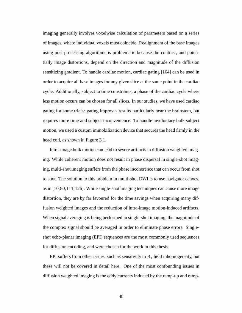
imaging generally involves voxelwise calculation of parameters based on a series

of images, where individual voxels must coincide. Realignment of the base images

using post-processing algorithms is problematic because the contrast, and poten-

tially image distortions, depend on the direction and magnitude of the diffusion

sensitizing gradient. To handle cardiac motion, cardiac gating [164] can be used in

order to acquire all base images for any given slice at the same point in the cardiac

cycle. Additionally, subject to time constraints, a phase of the cardiac cycle where

less motion occurs can be chosen for all slices. In our studies, we have used cardiac

gating for some trials: gating improves results particularly near the brainstem, but

requires more time and subject inconvenience. To handle involuntary bulk subject

motion, we used a custom immobilization device that secures the head firmly in the

head coil, as shown in Figure 3.1.

Intra-image bulk motion can lead to severe artifacts in diffusion weighted imag-

ing. While coherent motion does not result in phase dispersal in single-shot imag-

ing, multi-shot imaging suffers from the phase incoherence that can occur from shot

to shot. The solution to this problem in multi-shot DWI is to use navigator echoes,

as in [10,80,111,126]. While single-shot imaging techniques can cause more image

distortion, they are by far favoured for the time savings when acquiring many dif-

fusion weighted images and the reduction of intra-image motion-induced artifacts.

When signal averaging is being performed in single-shot imaging, the magnitude of

the complex signal should be averaged in order to eliminate phase errors. Single-

shot echo-planar imaging (EPI) sequences are the most commonly used sequences

for diffusion encoding, and were chosen for the work in this thesis.

EPI suffers from other issues, such as sensitivity to B�

field inhomogeneity, but

these will not be covered in detail here. One of the most confounding issues in

diffusion weighted imaging is the eddy currents induced by the ramp-up and ramp-

48

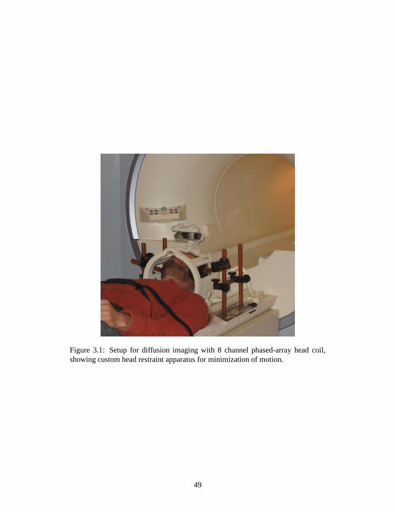
Figure 3.1: Setup for diffusion imaging with 8 channel phased-array head coil,showing custom head restraint apparatus for minimization of motion.

49

Figure 3.2: Eddy current induced artifacts in diffusion weighted images. Note thepronounced stretching of the brain in the phase encoding (anterior-posterior) direc-tion.

down of the large diffusion sensitizing gradients [2]. EPI is particularly susceptible

because of the low readout bandwidth in the phase encoding direction. The eddy

current induced magnetic field variations can be decomposed into a constant B�

shift, first order gradient fields along the x, y, and z axes, and higher order gradient

fields. In EPI, this results in a number of image artifacts. A B�

shift results in an

image shift in the phase encoding direction. A gradient in the readout direction

will cause a shearing of the image; in the phase-encoding direction, a compression

or stretching of the image; and in the slice select direction, reduction in the image

intensity due to imperfectly refocused spins [209]. These artifacts are illustrated in

Figure 3.2, which shows base diffusion weighted images with diffusion encoding

gradients in different directions, with no eddy current correction. Note the pro-

nounced stretching of the brain in the phase encoding (anterior-posterior) direction.

Like motion, these distortions are a problem when calculating voxelwise parametric

maps.

There are a number of approaches for dealing with eddy current induced ar-

50

tifacts. These include direct sequence modifications to reduce the residual eddy

currents at the time of the readout and post processing of the data to remove phase

errors due to the eddy current induced fields. The former have been shown to be

more effective, while using both can virtually eliminate artifacts [89]. Direct meth-

ods include the addition of pre- and post- gradient pulses and bipolar diffusion

encoding gradients in order to offset eddy current effects [6, 29, 74, 135, 158]. In

addition to phase correction approaches for dealing with eddy currents [29, 79], a

comprehensive approach for correcting eddy current and motion induced artifacts

has recently been proposed [159]. For the work in this thesis, the twice-refocused

balanced echo (TRBE) sequence of Reese et. al. [74,158] was implemented. In this

approach, the single diffusion encoding gradient lobes of the traditional Stejskal-

Tanner PGSE sequence (Figure 2.2.1) are replaced by bipolar gradients with a 180�

pulse in the centre (Figure 3.3). The effect for diffusing spins is the same as in the

PGSE sequence, but the opposite polarity of the bipolar lobes allows the eddy cur-

rent effects to be negated. If the eddy current decay time constant # is known, the

lobe lengths�1...�4 can be adjusted so that the residual current is zero, with the re-

quirement�1+�2=�3+�4. For our earlier studies [31], we implemented this scheme

on a 1.5T Siemens Magnetom Vision scanner (Siemens Medical Systems, Erlan-

gen, Germany). For our later work, we used a Siemens 1.5T Sonata scanner, with

the scheme already implemented. The timing used was�1=14410 � s,

�2=21950

� s,�3=24490 � s, and

�4=11870 � s.

A final issue with diffusion imaging is the low signal to noise ratio due to the de-

liberate signal reduction inherent in diffusion weighting. As a consequence, voxel

sizes need to be relatively large for diffusion imaging. We used an eight-channel

phased-array coil for improved SNR. With this coil, parallel imaging techniques

such as sensitivity encoding (SENSE) [154] may be used, enabling shorter echo

51

G

G

G

G

90 180 180o o

TE/2

o

δ1 δ2 δ3 δ4

Figure 3.3: Twice-refocused balanced echo (TRBE) diffusion encoding sequence.

times and hence increased SNR. However, SENSE reconstruction, as currently im-

plemented, was found to be too computationally expensive for stable routine use

with the available processor.

3.1.1 Diffusion tensor imaging

For diffusion tensor imaging, we made modifications to the Siemens TRBE se-

quence in order to loop through arbitrarily many diffusion encoding directions.

The directions were isotropically positioned in space: isotropic gradient direc-

tions have been shown to be optimal for tensor calculation [73, 83], and it has been

shown that for the purpose of signal averaging, instead of averaging the same direc-

tion, it is preferable to measure different directions for tensor reconstruction in the

brain [83, 132]. The gradient directions were calculated using an in-house electro-

static repulsion algorithm similar to that in [83]. The directions were randomized

for acquisition. In practice, we acquired up to 90 encoding directions for the full

52

brain, and up to 500 directions for single-slice data, with our current processors.

We used a b-value of 1300 s/mm � , which provides optimal signal to noise ratio in

the computed parametric maps [81], and 2.5 mm isotropic, contiguous voxels. We

fitted the diffusion tensor using least squares linear regression implemented with

Matlab�

software [108].

3.1.2 High angular resolution diffusion imaging

To compute the diffusion ODF at high angular resolution, we used q-ball (QB) re-

construction. The QBI reconstruction method was chosen because a model-free

reconstruction method was desired, it has been shown to be able to elucidate com-

plex tissue structure in the human brain [181], and it is relatively computationally

efficient. As described in Section 2.2.6, an approximate value of( � � � is given by

the Funk Radon transform of the signal [181]:

( � � � � ��

��

� � � � � � � � (3.1)

where � � � � represents the diffusion weighted signal strength measured with � �

� � � . We used b=3000 s/mm � , q=0.35 � m �� , and 2.8 mm isotropic, contiguous

voxels. We acquired 30 slices and used 90 isotropically spaced diffusion encoding

directions (see Figure 3.4). This QBI acquisition is of significantly lower angular

resolution than the 492-direction scheme introduced by Tuch et al., but the 90-

direction scheme was deemed sufficient to see multiple fibre crossings and made

a full-brain acquisition feasible in a clinically acceptable scanning time (roughly

15 minutes). The full width at half maximum of the Bessel kernel was 8.6 � � .

We note that higher q values and higher N could be used to measure the ODF at

�The QBI acquisition protocol described here has been published as a conference abstract [32].

53

Figure 3.4: Diffusion encoding directions generated using electrostatic repulsionalgorithm: 90 direction scheme used for full brain q-ball imaging. The directionsare spaced isotropically over a half sphere in q-space.

higher angular resolution, and the angular resolution required for some specific

applications could be higher.

Figure 3.5 shows the base diffusion weighted images acquired with this proto-

col. Note that the more striking signal difference, as the diffusion encoding gradi-

ent direction changes (e.g., goes from parallel to perpendicular to a fibre direction),

compared to that at lower b values (see Figure 2.3), allows for calculation of high

angular resolution detail in the diffusion pdf.

Figures 3.6 and 3.7 show the diffusion ODF calculated using the QBI and DTI

reconstruction approaches in the human brain. The region shown in Figure 3.6

shows partial volume averaging of the corpus callosum and the superior longitudinal

fasciculus, while Figure 3.7 shows partial volume averaging of fibre directions in

54

a b

c d

Figure 3.5: Base diffusion weighted images for QBI reconstruction with gradientsapplied in different directions, b=3000 s/mm � . Note the low SNR on average, andthe increased signal difference when the diffusion gradients are applied parallel andperpendicular to white matter fibres, as compared to Figure 2.3, which shows thebase images with b=1300 s/mm � . In these images, the diffusion encoding direc-tions are approximately (a) bottom left to top right (b) top left to bottom right (c)throughplane (d) left to right.

55

the cortical margin. The figures illustrate the additional information that can be

gained from QBI reconstruction: note that in cases where two fibres cross, the

tensor-derived ODF is planar, whereas the QBI ODF has clear maxima along the

fibre directions. Where the crossing is not orthogonal, the maximum of the tensor-

derived ODF does not lie along either direction.

In addition to the ODF shapes shown in Figures 3.7 and 3.6, we calculated a

model-free anisotropy index for the HARD data. We based the generalized frac-

tional anisotropy (GFA) on the fractional anisotropy used in DTI:

GFA �� ( � � �%� � & � � � ( � � �

� ( � � �� (3.2)

This is similar to the spherical diffusion variance defined by Frank [61]. Figure

3.8 compares the two measures for the same b=3000 s/mm � dataset. As expected,

the GFA measure is slightly more noisy than the FA: this can be seen qualitatively

by examining the grey matter, which is expected to have uniform, low anisotropy.

The two anisotropy maps, however, are very similar, confirming that the QBI re-

construction method is able to capture the anisotropy in the major fibre tracts. It

may be able to show increased anisotropy in regions of partial volume averaging of

tract directions, where the tensor defined ODF is relatively isotropic.

3.2 Anisotropic diffusion phantom

Fibre tractography using diffusion MRI data has the potential to provide very use-

ful information about neuronal pathways in healthy and diseased brain, however,

it can also reconstruct incorrect pathways (“false positives”) and miss legitimate

pathways (“false negatives”) due to problems with the diffusion pdf model used,

limitations of the tracking algorithm, and limitations and artifacts in the MRI ac-

56

a

b c

Figure 3.6: Estimation of the fibre orientation likelihood distribution: insets showthe diffusion ODF for (b) QB and (c) DT data in a region of partial volume aver-aging of fibre directions in the human brain. Note the ODF in the topmost voxelin (b) and (c), which has a planar shape in (c) but clearly indicates subvoxel cross-ing in (b). The shapes have been squared and renormalized in order to accentuateanisotropy for visualization purposes. The rectangle in the RGB plot shown in (a)indicates the region for which the diffusion ODF shapes are plotted. The insetshave been rotated relative to the RGB plot in order to show the directions clearly.The RGB plot is shown in order to indicate the direction of maximal diffusion ascomputed with DT reconstruction: red represents the component of the principaleigenvector of the diffusion tensor in the left-right direction, green the component inthe anterior-posterior direction, and blue the component in the head-foot direction.The region shown contains fibres from both the corpus callosum and the superiorlongitudinal fasciculus.

57

a b

c d

Figure 3.7: Diffusion ODF computed using (a,c) QBI and (b,d) DTI reconstructionin an area of complex neuronal architecture in the cortical margin. (a) and (b) showthe ODFs in the region indicated in the anatomical images at the top, and (c) and(d) are zoomed versions of the ODFs in the boxes shown in (a) and (b). The ODFshapes have been squared and renormalized in order to accentuate anisotropy forvisualization purposes, and the insets in (c) and (d) have been rotated slightly inorder to show the directions clearly. Note that in cases where two fibres cross, thetensor-derived ODF is planar, whereas the QBI ODF has clear maxima along thefibre directions. Where the crossing is not orthogonal, the maximum of the tensor-derived ODF does not lie along either direction.

58

Figure 3.8: LEFT: Generalized fractional anisotropy (GFA) and RIGHT: fractionalanisotropy (FA) maps generated using the same dataset with b=3000 s/mm � .

quisition. There is therefore a need to quantitatively evaluate tracking algorithms

to see to what extent they perform correctly and when they can be more or less re-

liable. Comparison to known human anatomy is an informative first step, however,

due to anatomical variability between individuals and our as yet incomplete knowl-

edge of human neuronal architecture, there is no “gold standard” connectivity map

for an individual human brain data set. Hence, it is difficult to do any quantitative

validation of human brain fibre tracking in vivo.

In Chapters 4-6, fibre tracking results will be presented in human brain datasets,

synthetic diffusion tensor datasets, formalin-fixed excised rat spinal cord, and fresh

excised rat spinal cord. The aim in all of these experiments is to investigate the

validity of the fibre tracking results. In this section, we will describe the motivation

behind these choices of datasets for fibre tractography validation.

Prior to the work described in Chapter 4, most fibre tracking results were an-

alyzed qualitatively by comparing in vivo human tractography results to known

human anatomy, specifically that known from post-mortem analysis [118]. Some

59

studies had been done in animal brain, such as that done in rats by Xue et al. [206].

Rat neuronal connectivity is less complex and more fully known than is human

connectivity, therefore qualitative comparison of tracking results can serve as vali-

dation. More recently, the tracking results achieved using diffusion imaging of the

rat have been compared to coregistered manganese-enhanced MRI of fibre tracts,

which gives excellent gold standard reference tracts [99]. These studies involved

anesthetizing the live animals and required a small animal scanner to achieve ad-

equate image quality. Alternatively, paraformaldehyde-fixed tissue from rodents

could be used, as was done by Ahrens et al. [3]. Studying fixed tissue is advanta-

geous because repeated studies can be performed without elaborate anesthetization

procedures. The tissue can be dissected afterward for comparison, or compared

to images of the tissue acquired using other modalities, such as fluoroscopy [188].

When we began our evaluation studies, validation using simulated data was becom-

ing more popular [94, 102, 177].

For evaluation of our preliminary tracking results, we used both simulated diffu-

sion tensor data and fixed, excised, rat spinal cord data scanned offsite in an animal

scanner. While the simulated data allowed us to investigate complex, branching

tract structure, it did not allow us to fully investigate the performance of the al-

gorithm in the presence of real imaging artifacts and noise characteristics. While

further simulation could be done to attempt to match these, we desired real MRI

data for full evaluation, and therefore also used the rat spinal cord data. The spinal

cord is a very simple structure in which to do fibre tracking, but was a good prelim-

inary validation step.

We investigated the potential of using fixed human cadaver brains to obtain DTI

data in our human scanner, as we did not have a small animal scanner onsite. Ca-

daver brain studies could be very useful for investigation of connections not yet

60

established to exist in humans: a very high quality, high resolution data set could

potentially be acquired, without cardiac and respiratory artifacts. Cadaver brains

could also potentially be used for routine tracking evaluation in complex human

anatomy using a human scanner, instead of requiring live subjects. Unfortunately,

there are many difficulties in scanning fixed tissue in a human MR scanner. For-

malin fixation changes the tissue structure significantly, so that the T � relaxation

times are significantly reduced and there is less free water to diffuse. The former,

compounded with the long echo times and deliberate reduction of signal necessary

to achieve diffusion weighting, causes the signal to noise ration of the base images

to be very low. The latter means that there is a smaller difference, as compared to in

vivo, in the diffusivity along different directions in anisotropic tissue (e.g., parallel

and perpendicular to fibres). In order to raise this difference above the noise levels,

higher b values are necessary, however, this leads to further reduction of the mean

signal.

We attempted both conventional spin-echo and EPI diffusion acquisitions on

cadaver brain with b=1800 s/mm � on a 1.5T Siemens Magnetom Vision MR scan-

ner. All results were of poor quality: an example diffusion tensor reconstruction is

shown in Figure 3.9. While the trace image is of acceptable quality (in our study,

the mean trace in the brain was 0.24E-6 � 0.16E-6 mm � /ms, including the formalin-

filled ventricles), the FA and principal eigenvector maps are only slightly better than

random noise. The trace, being the average of the three eigenvalues of the diffusion

tensor, is more robust to noise than are the eigenvectors and the anisotropy index,

which is a function of the three eigenvalues. Additionally, while the anisotropy

index in fixed and unfixed excised tissue has been shown to be the same [171],

it has been proposed that the FA drops post-mortem due to a lack of active pro-

cesses [202]. The direction maps achieved in our cadaver imaging studies were of

61

insufficient quality to do fibre tractography. More recent work [150] has corrobo-

rated these findings that diffusion imaging in fixed tissue using human scanners is

difficult. In high-field animal scanners equipped with very high gradients, the SNR

problems related above can be overcome.

A logical step after in vivo rat scanning is to scan nonhuman primates, as has

recently been done in the macaque [138]. Macaque neuronal connectivity is very

well known from tracer studies [149] and its complexity more closely resembles

that of humans than does that of rats. Macaque brains are larger than those of rats

and therefore do not require as sensitive a scanning device. We made some attempts

at validation in the macaque (shown in Figure 3.10), with the goal of comparing

fibre tracking results to the results of radioactive tracer studies in the same animal.

Unfortunately, the data quality from our 1.5T human scanner was of very poor

quality, primarily because the smaller size of the macaque brain necessitates smaller

voxel size, which compromises the SNR to too great an extent. The data shown

here are from a one hour DTI session with 2mm isotropic voxel size. A 0.5mm

isotropic resolution T � weighted anatomical scan was acquired in the same session

for a total scan time of 2 hours. It was difficult to keep the animal under general

anesthesia any longer than this. The fibre tracking results shown are for a large fibre

system (the pyramidal tract). The tracer tracking studies were being done for more

subtle cortico-cortical connections, for which the data quality and voxel size were

not suitable, hence, it was not possible to compare tracking results to the results of

these tracer studies.

For the study that will be presented in Chapter 6, we decided to construct a

physical phantom for fibre tracking validation using a 1.5T human MR scanner.

Desirable qualities for this phantom were anisotropic diffusion properties compa-

rable to those in human brain in vivo and complex, known fibre configurations of

62

Figure 3.9: Coronal slice of diffusion tensor images of formalin-fixed cadaver brain.CLOCKWISE FROM TOP LEFT: T � weighted (b=0 s/mm � ) image, FA, trace, andvector map of e � direction overlaid on FA map.

63

Figure 3.10: Fibre tracking in the macaque brain using a 1.5T human scanner.LEFT: tracking results for seeds placed in the pyramidal tract. RIGHT: T � weightedimage of the corresponding anatomy.

subvoxel curvature and fibre crossing. The phantom must have structure that re-

stricts or hinders water diffusion on a length scale we can probe in a diffusion MR

experiment, i.e., 10-50 � m. We first investigated the possibility of using commer-

cially available microtubing, however, the smallest dimensions available were 50

� m inner diameter and 325 � m outer diameter. The inner diameter is suitable for

imaging the “intracellular” diffusion compartment, however, the thick walls cause

the following problems: with the tubing packed as tightly as possible in a water-

filled container, (a) there is more wall than water in the phantom, leading to poor

SNR, and (b) the “extracellular” water compartment is much larger than the “in-

tracellular” compartment, and it is not sufficiently hindered on a scale compatible

with MR imaging. Microtubing is really only suitable for non-imaging studies us-

ing sensitive spectrometers, where the signal from filling only the “intracellular”

compartment is sufficient, and magnetic susceptibility induced imaging errors due

64

to air present in the scanning volume are not a concern. Such studies have been done

to explore the nature of the ADC profile [189] to confirm that the maxima of the

diffusion pdf measured using DSI match the fibre directions in a multi-directional

array of tubing [101].

Following our investigation of the suitability of microtubing, plants with ori-

ented fibrous structure were considered for the phantom. Celery and sunflower

stalks were scanned, but the resulting anisotropy index maps showed isotropic ma-

terial only: the restrictive barriers in these plants are not on a scale compatible with

a diffusion MRI experiment.

For the final phantom construction, it was decided to use fresh excised spinal

cords of rats. The white matter tracts in the cords are of approximately the same size

as white matter fibre pathways in the human brain, and exhibit similar properties of

anisotropy and intra-extracellular compartment permeability. They contain macro-

molecules that produce the same average ADC as in human white matter. Multiple

cords could be arranged in complex fibre geometries. The phantom design is dis-

cussed in Chapter 6 and shown in Figures 6.2 and 6.1. The cords were embedded in

2% agar, which kept them from moving and had suitable relaxation times for MRI.

2% agar solidifies at approximately 40�C, meaning that it could be poured over the

cords just before solidifying without damaging the tissue. The cords were scanned

shortly after they were excised, because autolyzation occurs within hours of death,

making further measurements of fibre structure difficult.

Subsequent to our experiments, a phantom composed of rayon has been pro-

posed [160]. Each rayon fibre is composed of 50 parallel micro-fibers whose di-

ameters are about 20 � m, creating anisotropic hindrance of diffusion on a scale

measurable by diffusion MRI. While promising, especially because of its reusabil-

ity, no complex fibre configurations have been scanned at this time.

65

Chapter 4

A geometric flow for white matter

fibre tract reconstruction

4.1 Preface

This chapter describes our first generation technique for fibre tracking with dif-

fusion MRI data. The goal was to address the issues that could confound other

existing fibre tracking algorithms: noise, subvoxel partial volume averaging of fi-

bre directions, and problems with the estimate of the diffusion pdf. Ultimately, we

desired an algorithm that could use diffusion tensor or high angular resolution data.

At the time this work was done, there were few practical HARD data acquisition

and postprocessing approaches for estimating the diffusion pdf, therefore as a be-

ginning step, the diffusion tensor was used. Instead of the streamline approaches

that existed at the time, we used a flow-based approach, which had the advantage

that it could reconstruct many branching tracts in parallel with no additional compu-

�This chapter is based on a published paper [33]. c

�2002 IEEE. Reprinted, with permission, from

J.S.W. Campbell, K. Siddiqi, B.C. Vemuri, and G.B. Pike. A geometric flow for white matter fibretract reconstruction. In Billene Mercer, editor, 2002 IEEE International Symposium on Biomedi-cal Imaging Conference Proceedings, pages 505–508. The Institute of Electrical and ElectronicsEngineers, Inc., Omni Press, 2002.

66

tational complexity as the number of tracts increased. Qualitative results are shown

in this chapter: extensive quantitative evaluation was not performed for this algo-

rithm due to the development of a clearly superior method, which will be described

in Chapter 5.

4.2 Introduction

In the central nervous system, the highly organized fibre structure of white matter

fibre tracts causes the diffusion of water molecules to be anisotropic, as described

in Chapter 2. With diffusion tensor imaging (Section 2.2.4), the direction and mag-

nitude of diffusion of water molecules is characterized by a diffusion tensor. The

tensor model is by far the most common description of the diffusion pdf, hence,

the reconstruction of continuous fibre tracts from such data is a problem of con-

siderable interest. In this chapter, we introduce a geometric flow to address this

problem. The key ideas are: (1) to locally extend the principal eigenvector field in

its orthogonal plane and (2) to model the fibres as very thin tubes, by introducing

a constraint on the minimum cross-sectional curvature. We illustrate the approach

with reconstructions of both simulated and real diffusion tensor images.

We have chosen a geometric flow to drive our fibre tracking algorithm be-

cause of its potential to reconstruct complex fibre configurations, such as branching,

crossing, and curvature. This algorithm is based on a flow originally designed for

the segmentation of blood vessels from magnetic resonance angiography (MRA)

data [185, 186]. Both vessels and fibre tracts can be modeled as thin tubes. The

initial step in the blood vessel segmentation algorithm is the creation of a vector

field from the scalar MRA images. It was thus reasonable to modify this algorithm

to accept as input vector data, specifically the principal eigenvector field from DTI,

instead of scalar data. The algorithm has the advantage that it can reconstruct many

67

tracts in parallel, instead of iteratively.

There is a growing computer vision literature on the use of geometric flows for

image segmentation. Most existing methods draw their motivation from the active

contour model of Kass, Witkin and Terzopoulos [85] but rely on level set techniques

introduced by Osher and Sethian to handle topological changes in a seamless fash-

ion [127]. The first such approach was introduced independently by Caselles et

al. [38] and Malladi et al. [104]. These models later evolved to include interpre-

tations as gradient flows that minimized particular weighted geometric function-

als [39, 86] and to take into account the statistics of the regions enclosed by the

evolving curves or surfaces [136, 207].

As described in Section 2.3, a few methods have recently been proposed in

the literature for reconstructing fibre tracts from DTI data [16, 115, 142, 183], but

each has one or more limitations. Fibre tract reconstruction remains a significant

computational challenge because the geometry of the fibre structures is typically

quite complex, with multiple fibres being very close to one another, and the MRI

measurements are also noisy. The issue of regularizing the data while preserving

its “structure” has been proposed as a solution to some of these problems (Section

2.2.5). The geometric flow introduced here assumes that the images have first been

suitably regularized. The key construction is to extend the principal eigenvectors

(locally) in the planes orthogonal to them and to then apply the flux maximizing

flow introduced in [186]. A further constraint on the cross-sectional curvature is

introduced to force the flow to give narrow structures, since one has the strong prior

knowledge that the fibre tracts should be tubular.

68

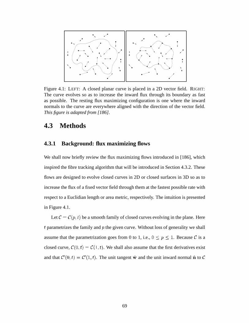
Figure 4.1: LEFT: A closed planar curve is placed in a 2D vector field. RIGHT:The curve evolves so as to increase the inward flux through its boundary as fastas possible. The resting flux maximizing configuration is one where the inwardnormals to the curve are everywhere aligned with the direction of the vector field.This figure is adapted from [186].

4.3 Methods

4.3.1 Background: flux maximizing flows

We shall now briefly review the flux maximizing flows introduced in [186], which

inspired the fibre tracking algorithm that will be introduced in Section 4.3.2. These

flows are designed to evolve closed curves in 2D or closed surfaces in 3D so as to

increase the flux of a fixed vector field through them at the fastest possible rate with

respect to a Euclidian length or area metric, respectively. The intuition is presented

in Figure 4.1.

Let� � � � � �� be a smooth family of closed curves evolving in the plane. Here

� parametrizes the family and the given curve. Without loss of generality we shall

assume that the parametrization goes from 0 to 1, i.e., �� . Because�

is a

closed curve,� � �� . We shall also assume that the first derivatives exist

and that� � � �� . The unit tangent

� and the unit inward normal�� to

�

69

are given by

� �

��

� �

��

� � � � ��

��

��

� �

��

� � � � ��

�� (4.1)

where � is the arc-length parametrization of the curve. Now consider a vector field � � � � � � � � � � � � �� defined for each point �� in � . The total inward flux

of the vector field through the curve is given by the contour integral

��

��

� � � �� (4.2)

where �� is the Euclidian length of the curve and �� denotes the inner product

of vectors a and b. In recent work [186], it was shown that the following result

holds:

Proposition 1. The direction in which the inward flux of the vector field

through

the curve�

is increasing most rapidly is given by �� .

In other words, the gradient flow which maximizes the rate of increase of the total

inward flux with respect to the Euclidian arc-length is obtained by moving each

point of the curve in the direction of the inward normal by an amount proportional

to the divergence of the vector field. To see this one can compute the first variation

of the flux functional with respect to the parameter � to get

��

�� !��

� � � �� !�

�

70

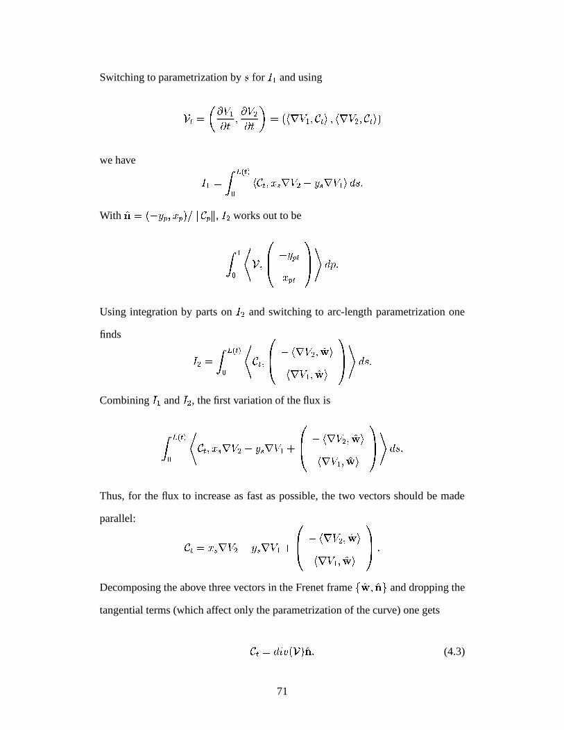
Switching to parametrization by � for � � and using

� �

� � ��

� ��

� � � � � � � � ��

we have � ��

� � � � � �� With

�� , � � works out to be

� ��

� �

��

� � �

� ��

Using integration by parts on � � and switching to arc-length parametrization one

finds

� � � ��

�

� ��

��

� ��

Combining � � and � � , the first variation of the flux is

� � ��

�

� ��

��

� � � � � � ��

Thus, for the flux to increase as fast as possible, the two vectors should be made

parallel:

��

��

� � � � � � ��

Decomposing the above three vectors in the Frenet frame � � � �� and dropping the

tangential terms (which affect only the parametrization of the curve) one gets

�� (4.3)

71

This result also generalizes to the case of an evolving closed surface�

in a 3D

vector field

:

Proposition 2. The direction in which the inward flux of the vector field

through

the surface�

is increasing most rapidly is given by �� .

The calculation, which will not be presented here, is similar to the one for 2D but

requires the use of properties of vector products and integration by parts on a double

integral.

4.3.2 A modified flow for fibre tract reconstruction

The flux maximizing flow is designed to align the evolving curve or surface to be

locally perpendicular to the vector field of interest. Thus it can be a very useful

tool in the segmentation of medical images. For example, in the segmentation of

magnetic resonance angiography (MRA) images the vector field can be taken to be

the gradient of the intensity image [186]. In DTI, at locations where the diffusion

is anisotropic, the principal eigenvector field gives the local orientation along white

matter fibre tracts. The key to applying the flux maximizing flow to such data is

to view the fibre tracts as very narrow tubes in 3D1 and to extend each element

of the vector field in the plane orthogonal to it, as illustrated in Figure 4.2. By

this construction one can seek an evolution that grows seeds along fibre tracts by

maximizing the inward flux of the extended vector field through their surfaces.

The principal eigenvectors of the diffusion tensor are extended in the plane or-

thogonal to them using the following procedure. First, let each voxel centered at

x in the original data set be represented by a 3x3x3 block of voxels in a new data

set. For each voxel in the 3x3x3 block centered at x in the new data set, construct

1In the limit as the thickness shrinks to zero one obtains a 3D curve.

72

Figure 4.2: Flux maximizing flow for fibre tract reconstruction using diffusion ten-sor data. The principal eigenvectors are shown as solid lines sweeping out a whitematter fibre tract (a 3D curve). Each eigenvector is extended locally in the plane or-thogonal to it. The extended vector field, shown by the arrows, is one which createsa large inward flux through the surface of a narrow tube.

the vector from that voxel to x and project this vector onto the plane orthogonal

to the principal eigenvector in the original voxel. Store the resulting vector at the

corresponding voxel in the 3x3x3 block. Finally, scale each stored vector by the

anisotropy index, which can be viewed as a measure of confidence in the direction

of the principal eigenvector. In our experiments, we use the fractional anisotropy

(Equation 2.29). The construction of the extended vector field is illustrated for two

of the planes in the 26-neighborhood of a point x in Figure 4.3.

Unfortunately, this construction is not by itself sufficient to reconstruct the tracts

reliably in the presence of noisy data. A few corrupted measurements can cause the

flow to ‘bleed’, i.e., to flow perpendicular to the actual tracts and to create blob-like

structures instead of tube-like structures. However, there is a strong prior on the

reconstruction we seek that can be exploited: the fibres are expected to be narrow

tubes. Thus one can invoke the powerful constraint that the maximum principal

curvature of the evolving surface (the one that lies in the plane orthogonal to the

principal eigenvector) should remain high. Thus one is lead to the following modi-

73

b)

y

z

a)

y

x

Figure 4.3: Construction of the extended vector field corresponding to to the prin-cipal eigenvector � � � � �� at a point x (x is the centre of the block). Theconstruction is illustrated for two planes in the 3x3 neighborhood of x. a) � � plane(orthogonal to � � ). b) � � plane.

fied flux maximizing flow for fibre tract reconstruction

� �� (4.4)

Here,�

is the evolving surface,�� is its unit inward normal, � � � � � are its principal

curvatures, � � is the expected minimum cross-sectional curvature of a fibre, and

is the extended vector field.

In order to implement the flow, we use the level set representation for surfaces

flowing according to functions of curvature [127] which is now a standard approach

for implementing partial differential equations of this type in the literature, since

it allows for topological changes to occur without any additional computational

complexity. Let� � � � � �� # � � � be a family of surfaces satisfying

the curve evolution equation�

� � � �� , where�

is an arbitrary (local) scalar speed

function. Then it can be shown that if� � � � � � �� is represented by the zero level set

74

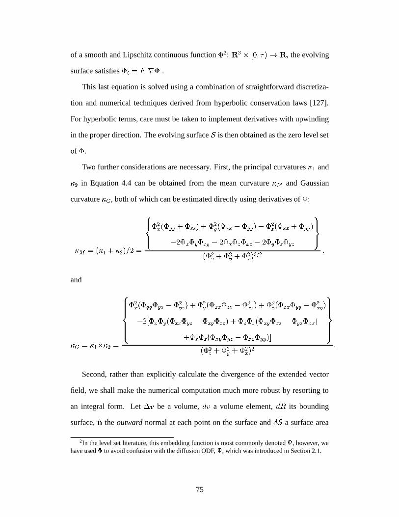
of a smooth and Lipschitz continuous function' 2: � � � �� # � � � , the evolving

surface satisfies'

� � � � � ' � .This last equation is solved using a combination of straightforward discretiza-

tion and numerical techniques derived from hyperbolic conservation laws [127].

For hyperbolic terms, care must be taken to implement derivatives with upwinding

in the proper direction. The evolving surface�

is then obtained as the zero level set

of'

.

Two further considerations are necessary. First, the principal curvatures � � and

�� in Equation 4.4 can be obtained from the mean curvature � � and Gaussian

curvature � � , both of which can be estimated directly using derivatives of'

:

��

�� ' �� ' � �� ' � � � � ' �� ' � � � ' � � � � ' �� ' � � � ' � � �� ' � ' � ' � � � � ' � ' � ' � � � � ' � ' � ' � �

��

� ' �� ' �� ' ��

and

��

�� ' �� ' � � ' � � � ' �� ' �� ' � � ' � � � ' �� ' �� ' � � ' � � � ' �� ' � ' � � ' � � ' � � � ' � � ' � � � � ' � ' � � ' � � ' � � � ' � � ' � � �

� ' � ' � � ' � � ' � � � ' � � ' � � �

��

� ' �� ' �� ' ��

Second, rather than explicitly calculate the divergence of the extended vector

field, we shall make the numerical computation much more robust by resorting to

an integral form. Let� � be a volume,

� � a volume element,� �

its bounding

surface,�� the outward normal at each point on the surface and

� �a surface area

2In the level set literature, this embedding function is most commonly denoted � , however, wehave used to avoid confusion with the diffusion ODF, � , which was introduced in Section 2.1.

75

element. Via the divergence theorem,

�� div � � � ��

�$ � � � �� (4.5)

In other words, the integral of the divergence of a vector field over a volume is given

by its outward flux through that region’s bounding surface. For our implementa-

tion, we use this flux formulation to implement the divergence term in Equation

4.4. Numerically, this operation is far more stable than attempting to estimate the

divergence via derivatives of the vector field

, particularly at locations where this

vector field is becoming singular. We calculate the flux through spheres of diameter

1.5 voxels in the extended vector field. Specifically, we calculate the flux at the

centres, corners, faces, and centres of the edges of the 3x3x3 blocks. This allows

us to measure the flux at a precise scale that is meaningful for the extended vector

field we have constructed: the extended vector field directions are changing rapidly,

and we wish to look at these changes from one voxel to the next.

4.4 Results

We now present experimental results on both synthetically generated data and DTI

vector field data from the spinal cord of a rat. Both data sets are stored in rectangular

3D lattices. The synthetic data were created by simulating random walks through a

rectangular lattice in 3D, while allowing for branching to occur. The superposition

of the vectors obtained by all the walks was considered to be the organized tracts to

be reconstructed. An anisotropy index of 1 was assigned to all of the voxels visited

by the random walks. Vectors of random orientation were assigned to voxels that

had not been visited by the random walk. These were assigned random anisotropy

indices less than one. This simulates unorganized tissue micro-structure in the re-

76

gion surrounding the tracts. The vector field thus obtained and the results of the

reconstruction process using the flux maximizing flow on the extended vector field

are shown in Figure 4.4 (the views are not precisely registered). The initial seeds

were placed automatically at voxels having high inward flux, however, the algo-

rithm could be seeded manually in order to start the tracking in a specific region of

interest.

The second data set was obtained from diffusion tensor imaging of the spinal

cord of a rat. The images were obtained in a small-bore magnet with a voxel size

of 70.31x70.31x200 � m . Prior to processing this data for reconstruction, it was

smoothed using the regularization flow proposed in [187].

Figure 4.5 shows the anisotropy index calculated from the rat data and the result

of the reconstruction. The white matter is the outer part of the cord, and is aligned

parallel to the cord direction in this part of the cord. Once again, the initial seeds

were placed at voxels having high inward flux. The results are shown as surfaces,

however, a thinning algorithm such as that described in [25] could be applied to the

reconstructed tubes in order to obtain 3D curves representing the tracts.

4.5 Discussion

We have presented a geometric flow for reconstructing white matter fibre tracts,

modeled as narrow tubes in 3D. The key benefit of our method is that it has the

ability to reconstruct multiple fibres in parallel, instead of taking an iterative ap-

proach. It handles arbitrary numbers of branches and merge points. The flow does

not stop when the anisotropy index falls below a threshold, although the speed of

flow is scaled by the AI in order to reflect our certainty in there being oriented

fibre structure in a given voxel. Removing this scaling may improve results in re-

gions where small tracts have low anisotropy due to partial volume averaging with

77

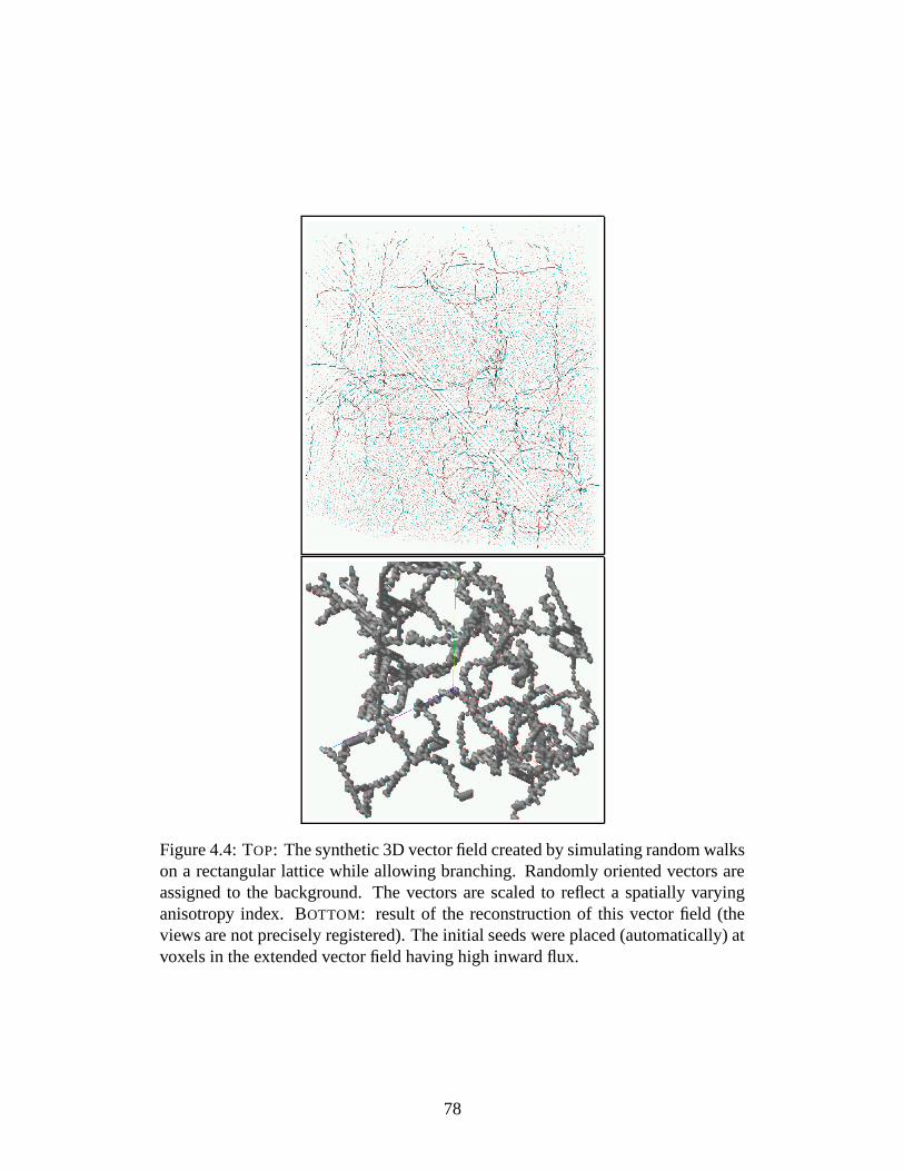
Figure 4.4: TOP: The synthetic 3D vector field created by simulating random walkson a rectangular lattice while allowing branching. Randomly oriented vectors areassigned to the background. The vectors are scaled to reflect a spatially varyinganisotropy index. BOTTOM: result of the reconstruction of this vector field (theviews are not precisely registered). The initial seeds were placed (automatically) atvoxels in the extended vector field having high inward flux.

78

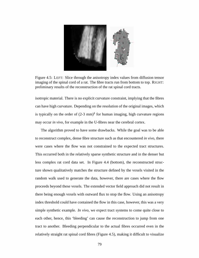
Figure 4.5: LEFT: Slice through the anisotropy index values from diffusion tensorimaging of the spinal cord of a rat. The fibre tracts run from bottom to top. RIGHT:preliminary results of the reconstruction of the rat spinal cord tracts.

isotropic material. There is no explicit curvature constraint, implying that the fibres

can have high curvature. Depending on the resolution of the original images, which

is typically on the order of (2-3 mm) for human imaging, high curvature regions

may occur in vivo, for example in the U-fibres near the cerebral cortex.

The algorithm proved to have some drawbacks. While the goal was to be able

to reconstruct complex, dense fibre structure such as that encountered in vivo, there

were cases where the flow was not constrained to the expected tract structures.

This occurred both in the relatively sparse synthetic structure and in the denser but

less complex rat cord data set. In Figure 4.4 (bottom), the reconstructed struc-

ture shown qualitatively matches the structure defined by the voxels visited in the

random walk used to generate the data, however, there are cases where the flow

proceeds beyond these voxels. The extended vector field approach did not result in

there being enough voxels with outward flux to stop the flow. Using an anisotropy

index threshold could have contained the flow in this case, however, this was a very

simple synthetic example. In vivo, we expect tract systems to come quite close to

each other, hence, this ‘bleeding’ can cause the reconstruction to jump from one

tract to another. Bleeding perpendicular to the actual fibres occurred even in the

relatively straight rat spinal cord fibres (Figure 4.5), making it difficult to visualize

79

the tubelike structures and making unconnected regions appear connected. In this

case, the bleeding was probably due to noise, however, we did not rule out fun-

damental issues with the extended vector field: in any case where there is not an

isolated pathway of voxels with inward flux, the flow will bleed, and it is possible

that the extended vector field construct resulted in such cases.

In this implementation, we scale the speed of the flow by the anisotropy index

in order to reflect our confidence in there being oriented fibre structure in a given

voxel. It may be informative to examine not only the final surface configuration,

but to use the speed at which the surface evolved to determine which reconstructed

tracts are most plausible. In cases, such as the synthetic dataset, where the back-

ground has low anisotropy, many of the incorrect pathways evolved more slowly

than the correct ones, by virtue of the definition of the speed function. Instead

of considering the reconstructed surface to be a binary map of connected and un-

connected voxels, we could use the speed of evolution to define a likelihood of

connection. However, the speed function used here is not an ideal solution: in cases

such as the rat spinal cord example, the flow evolved in the wrong direction within

a large region of high anisotropy, i.e., incorrect connections evolved quickly. In the

next chapter, we will present a modified speed function that can be used to define a

likelihood of connection between any two points.

Our discussion has so far focused on the reconstruction of fibre tracts from the

principal eigenvector field derived from the diffusion tensor. The tensor formulation

is limited because of its assumption that the diffusion is Gaussian. This assumption

breaks down in regions where fibres cross at a sub-voxel scale, or where the dif-

fusion is highly restricted. In the case of crossing fibres, the tensor gives only

volume-averaged information about the direction of fibres, and the AI is artifactu-

ally low. It may be preferable to use all of the information in the diffusion tensor

80

instead of only the principal eigenvector. Even greater accuracy for fibre orienta-

tion could be obtained by measuring the diffusion displacement distribution at high

angular resolution, as described in Section 2.2.6. Our method could potentially be

modified to use such diffusion measurements made using arbitrarily high angular

resolution: this would be a key advantage of this algorithm over other fibre tracking

techniques.

In summary, this approach could benefit from the following: (1) an alternative to

or improvement on the extended vector field approach, which in some cases did not

have the desired result due to discretization issues, (2) a measure of our confidence

in the existence of the reconstructed tracts, and (3) a method for handling high

angular resolution diffusion data.

81

Chapter 5

Flow-based white matter fibre

tractography and scalar connectivity

assessment using fibre orientation

likelihood distribution

5.1 Preface

In Chapter 4, we introduced a geometric flow for white matter fibre tract recon-

struction. While the flow-based approach to tractography was promising, this algo-

rithm had several distinct disadvantages, as described in section 4.5. The expanded

vector field was cumbersome, and added to the computation time. The initial im-

plementation used only the principal eigenvector of the diffusion tensor, which can

be problematic in many scenarios which arise in vivo, such as fibre crossing. It

was unclear whether this flow had any significant advantages over streamline al-

�This chapter is based on two published abstracts [31,32] and a paper that has been submitted to

NeuroImage.

82

gorithms using the principal direction of diffusion. A suitable implementation for

HARD data, with the exception of the simple case of extracting the direction of the

peak of the diffusion pdf measured with such methods, was not described. In this

chapter, we introduce another geometric flow that addresses these issues. It gives

us both a connection from any point A to any point B as a 3D curve, as well as

a scalar measure of our confidence in the existence of this connection. It uses the

full diffusion ODF obtained from either diffusion tensor or, if available, high angu-

lar resolution diffusion data. Qualitative results in human brain are shown in this

chapter, and quantitative evaluation will be presented in Chapter 6.

5.2 Introduction

The first work on 3D fibre reconstruction in the CNS used diffusion tensor (DT)

data, so named because it is obtained by modeling the diffusion pdf as an anisotropic

3D Gaussian function, which can be described by a second order tensor [15]. The

reconstruction of tracts was done by curve propagation using the principal eigenvec-

tor of the diffusion tensor [16, 115, 188]. Such principal diffusion direction (PDD)

techniques can be confounded when there is more than one fibre direction within

a single imaging voxel. With voxel sizes typical of diffusion acquisitions (10-30

mm ), there is significant partial volume averaging of fibre directions in anatomi-

cal regions of both research and clinical interest, such as the association fibres near

the cortex. This partial volume averaging may be due to high curvature, crossing,

branching, or splaying of tracts.

A number of solutions have been proposed to deal with the problem of subvoxel

partial volume averaging of fibre directions. While going to smaller and smaller

voxel size can be advantageous, SNR soon becomes too low and the additional scan

time required to get sufficient signal impractical. Alternatively, the diffusion tensor

83

itself contains information about multiple subvoxel fibre directions: for example,

when the fibres are restricted to a plane, a level set of the tensor-described diffu-

sion pdf is a planar ellipsoid. Although the principal eigenvector direction may

not reflect the fibre directions in this case, the full tensor may be used for track-

ing, as has been proposed by several groups [17, 31, 95, 125]. Alternatively, given

sufficient diffusion weighted images (DWIs), bootstrap methods may be used to

estimate confidence intervals or a marginal posterior distribution for the direction

of the principal eigenvector [20, 82]. Although the full tensor does give us more

information than its principal eigenvector alone, there has recently been increasing

interest in forgoing the classic tensor description of the diffusion pdf in favour of

high angular resolution diffusion (HARD) pdf reconstruction to infer multiple fibre

directions within single voxels. HARD reconstruction techniques were described

in detail in Section 2.2.6: they include multi-tensor modeling [184], diffusion spec-

trum imaging to estimate the full 3D diffusion pdf using q-space methods [197],

and model-free extraction of the radially persistent angular structure using either

maximum entropy solutions [8] or modified q-space methods [181]. Addition-

ally, regularization techniques can be used to infer multiple fibre directions from

a single-tensor field [48, 157].

In this chapter, we describe a new fibre tracking algorithm that uses the full dif-

fusion pdf estimated with either HARD or DT techniques. The algorithm, which we

have named Tracking Using Fibre Orientation Likelihood Distribution (TUFOLD),

is a modification and extension of Fast Marching Tractography (FMT) [143], and

is a continuation of our earlier work on flow-based tractography [31, 33]. We show

fibre tracking results using both HARD and DT data in the human brain, and in-

troduce a novel hybrid approach that combines the two types of data in order to

capitalize on the advantages of each approach.

84

5.3 Methods

5.3.1 Flow and assignment of likelihood of connection

Our approach to tractography is a surface-evolution scheme driven by an estimate

of the fibre orientation likelihood distribution, �� , which could describe multiple

sub-voxel fibre directions. � � gives us a measure of our confidence that a fibre

exists in the direction of the unit vector � � � � � � � & � , at each spatial position x, and

shall be denoted � � � � � � � . Let� � � � �� be a surface with initial value

� � � � � �� given

by the boundary of a user-defined seed voxel or region.�

is evolved outward with

speed�

along its normal,�� %� � & � � :

� ��

�� (5.1)

� � � � �� is set equal to our confidence that a tract exists in the direction�� , i.e., the

fibre orientation likelihood distribution value in direction�� at position � in the MRI

volume:

� � � � �� (5.2)

As in Chapter 4, we use the level set techniques of Osher and Sethian [127] for

surface evolution. The surface�

is embedded as the zero level set of a 3D function'

. The evolution is given by � �� ' � , where the initial value of

'at any

point is the signed Euclidian distance from the point to the edge of the seed region.

The propagation of�

is equivalent to simultaneously propagating a continuous

field of curves outward from the seed� �

. As�

passes through a voxel, a time

of arrival�

is assigned to that voxel.�

is the solution of the Eikonal equation,

� � � � � � � . To calculate putative tracts as 3D curves, we retrace the path of

85

a b c

Figure 5.1: 2D schematic of flow-based surface evolution tractography. (a): Theinput data consists of the fibre orientation likelihood distribution � � defined at eachvoxel (the voxels with no shape shown represent voxels with isotropic diffusion,hence no fibre structure). The user defines a seed region, and a surface

�is initial-

ized to be the outer edge of the seed region (� �

). (b): the surface evolves at speedF along its normal

�� , with�

given by the value of � � in the direction of�� . As�

evolves, a scalar map�

of the time of arrival of the surface is constructed. (c):Gradient descent through the time of arrival map (shown as greyscale) gives thefibre tract reconstructions as curves.

normals to�

that led to each voxel reached: this path is given by gradient descent

through the map of the time of arrival of the surface,� � � � , from each point x to the

seed. Figure 5.1 shows a schematic of the tracking algorithm. We note that in the

limit where the estimated fibre orientation likelihood distribution becomes a delta

function (nonzero along only the maximum of the diffusion pdf), TUFOLD reduces

to standard streamline curve propagation.

In order to quantify our confidence in the existence of each reconstructed tract,

we define the likelihood of each tract’s existence, � � . We have a discrete array� �

of speed function values at each step along each tract. We smooth the array

with a one dimensional Gaussian kernel with a full width at half its maximum of

three voxels. This step is essentially a regularization step that reduces sensitivity to

isolated corrupted voxels by blurring only along the tract direction. We define � � to

86

be the lowest value in the smoothed array of speed functions values:

�� min � � � � � (5.3)

�� is a measure of our certainty in a tract’s existence given the measurements we

have made. It reflects uncertainty due to partial volume averaging of tract directions

in cases of crossing, branching, curvature, and tracts forming a “bottleneck”; partial

volume averaging of fibres with isotropic material, which leads to low anisotropy;

and imaging noise, which can confound the fibre directions. � � gives a relative cer-

tainty in the existence of all tracts reconstructed through one seed voxel or region.

The likelihood function given in Equation 5.3, even with the blurring of the

array of F values, gives a measure of the worst-case tract certainty on a local scale,

i.e., if there is one local region of low F values, the certainty in the tract will be

low, and this gives us no information about the F values along the rest of the tract

on a global scale. This makes sense, because we cannot have more certainty in a

tract’s existence than we do in its worst-case segment. A likelihood measure should

meet two criteria: first, we should compute the same value if we compute � � on

a curve starting at point A and going to point B as we would starting at B and

going to A, and second, given a point C between A and B, we cannot have higher

confidence in B being connected to A than we do in C being connected to A. While

we explored the possibility of computing other likelihood functions that provided a

balance between global and local tract properties, these two criteria eliminated all

but the worst-case measure.

We use stopping criteria based on both the value of the fractional anisotropy

(FA) [151] (see Equation 2.29) and the tract curvature. The speed function is set to

zero when FA � 0.1, and � � is set to zero if the tract curvature from voxel to voxel

(calculated after the gradient descent step) exceeds 80�. The FA threshold of 0.1

87

should allow tracking through regions of low anisotropy such as deep gray matter

matter structures, but should stop the flow in voxels with isotropic diffusion, for

instance, the ventricles [138]. We note that the algorithm can accept user-defined

stopping criteria that vary throughout the brain in order to make use of a priori

knowledge as to the nature of the fibre pathways.

Optionally, a Bayesian classifier may be used to segment out tissue (or white

matter only, if desired) prior to tracking [56]. Alternatively, the base diffusion

weighted images can be thresholded to confine the tracking to the brain.

We note that TUFOLD is similar to the Fast Marching Tractography (FMT)

method previously described by Parker et al. [143]. The differences are that TU-

FOLD (a) is applicable to either tensor or high angular resolution diffusion mea-

surements and (b) uses the fibre orientation likelihood distribution, instead of the

principal eigenvector of the diffusion tensor. In parallel with our work, a similar

front evolution scheme using the fibre orientation likelihood distribution has been

described by Tournier et al. [176]. It does not return explicit tracts as 3D curves, but

only an index of likelihood of connection, and has not been applied to HARD data.

The tracts and likelihoods of connection achieved through the surface-evolution

process of TUFOLD should be similar to those obtained by a Monte Carlo or itera-

tive tracking approach such as those described in [20,21,69,90]. Such methods have

not been applied to HARD data. Additionally, with surface evolution, the propa-

gation of all the curves is simultaneous and continuous, and therefore potentially

faster, especially as the number of putative paths increases.

88

5.3.2 Estimation of the fibre orientation likelihood distribution

from the diffusion data

Essential to our fibre tracking algorithm is an estimate of the likelihood that a fibre

is oriented in direction � � � & � : the fibre orientation likelihood distribution, � � � � � & � .We begin with an estimate of the diffusion pdf, given either by diffusion tensor

data, in which case the pdf is modeled as a 3D Gaussian function, or high angular

resolution diffusion pdf estimates, in which case the pdf does not a have predefined

functional form. We then compute the diffusion ODF,(

, which is the normalized

projection of the 3D diffusion pdf on the surface of the unit sphere (see Equation

2.11). Next, we estimate the fibre orientation likelihood distribution, as distinct

from the diffusion ODF.

Extraction of � � from the diffusion ODF consists of deconvolving the diffusion

ODF with the single-fibre response function. However, the single-fibre response

function is not known. The exact mechanisms responsible for the observed white

matter diffusion signal are still being investigated. The response to a single fibre

can be expected to change throughout the white matter in the brain, due to mi-

crostructural differences between, for example, association and commissural fibres,

and could also change in the presence of pathology. Hence, estimating the fibre

orientation likelihood distribution involves some degree of modeling and simplifi-

cation. We simplify the problem by assuming that the single-fibre response function

is a delta function in the direction of the fibre, i.e., we use the diffusion ODF as an

estimate of � � . We further threshold the ODF at its mean in order to restrict flow in

regions of isotropic diffusion:

� � � � � =( � � � if

( � � � � 1

= 0 if( � � � � 1 .

(5.4)

89

Figure 5.2: Thresholding the diffusion ODF: the threshold of �� 1 is in place toeliminate the case, possible in regions of high curvature, where the flow from pointA reaches point B by path ii or iii before path i.

The threshold of the diffusion ODF at its mean should also stop flow perpendicular

to single-fibre directions. In the case of a single fibre in each voxel, there will

be low but non-zero diffusion perpendicular to the fibre direction, and flowing in

this direction could impede the reconstruction of highly curved tracts, as shown in

Figure 5.2. We wish to be able to track through structures with low anisotropy, such

as the thalamus and regions near the cortex, therefore a threshold of significantly

greater than 1 is also undesirable. The more anisotropic the underlying diffusion

pdf, the smaller the solid angle in which � � is nonzero, which is what we desire.

While the assumption that the single-fibre response function is a delta function

is known to be an oversimplification, the �� estimated in this manner has the prop-

erty that it has higher values along fibre directions, as has been shown in q-space

validation studies using simple synthetic systems with partial volume averaging of

fibre directions [101], and is relatively simple to calculate for tracking purposes.

This estimate of � � is easily calculated for both DT and HARD data, which is ex-

tremely beneficial when combining the two types of ODF reconstruction for track-

90

ing.

In many cases in the human brain, we can expect the diffusion tensor model to

be adequate, and the use of HARD data may increase susceptibility to noise-induced

artifacts because it is model free, whereas the tensor ODF can be described with

only five parameters. When HARD data are available, we propose to first calculate

the diffusion tensor, and only use the HARD data for estimation of � � in cases

where the diffusion tensor model fits the data poorly. We do this by calculating the

� � statistic for the linear regression used to calculate the diffusion tensor, and using

HARD reconstruction when� � � � � � � � �� [153]. " is estimated by measuring

the mean of the signal intensity in a region outside of the object being imaged and

multiplying by� � � �

[76]. The �� map calculated in the human brain is shown in

Figure 5.3. In this case,� � � � � � � � � � � corresponded to �� . The threshold

of� � � � � � � � �� is low and gives preference to QBI reconstruction. Regions of

low � � corresponded to the larger fibre tracts, e.g., much of the corpus callosum and

the pyramidal tracts. � � was extremely high in CSF: this is because with b=3000

s/mm � , the diffusion weighted signal was very close to the noise floor for CSF,

which has a high apparent diffusion coefficient due to lack of restrictive barriers.

The �� value should be disregarded in these voxels, and was by use of a tissue

mask that excluded CSF.

We use q-ball imaging (QBI) to obtain high angular resolution estimates of the

diffusion ODF [181] (see Sections 2.2.6 and 3.1.2). We shall refer to the TUFOLD

algorithm run with diffusion tensor data as TUFOLD-DT, the TUFOLD algorithm

run with QBI data only as TUFOLD-QB, and the TUFOLD algorithm run with

diffusion tensor data where the diffusion tensor fit is good and QBI data elsewhere,

will be called TUFOLD-HYBRID.

Using � � , as defined in Equation 5.4, allows the evolving surface�

to flow

91

Figure 5.3: � � map for diffusion tensor fit in the human brain. � � is high in voxelswhere there is highly oriented fibre structure (e.g., the corpus callosum), but is lowin regions where there may be partial volume averaging of diffusion compartments.

through regions where there is ambiguity or low confidence in fibre direction: for

example, regions of partial volume averaging of fibre directions due to subvoxel

crossing, ‘bottlenecks’, or bending; regions of partial volume averaging of isotropic

grey matter and fibre structure (e.g., the thalamus); or voxels corrupted by noise

and/or imaging artifacts (where the pdf maximum may be slightly shifted from the

correct direction). The speed of propagation is simply reduced in these regions,

and the ambiguity at these points will be reflected in the likelihood measure. When

diffusion tensor measurements are used, �� is suitable even when there is partial

volume averaging of fibre directions: when there are multiple fibre directions in one

plane, the tensor will be “flat”. The fibre direction within this plane is unknown,

and the fibre orientation likelihood distribution will reflect this by being nonzero

everywhere in this plane, and zero outside of it. However, HARD data can be

useful for refining the speed function further by giving it clear maxima along the

fibre directions in the case of fibres crossing within a voxel. This refinement can

make the flow more controlled and more accurate, especially in cases where the

maximum of the tensor-described ODF does not lie along either fibre direction.

92

� � estimated from HARD data will be similar to that from DT data in the case of

subvoxel curvature, where a continuum of directions exists within a single voxel.

We note here that other methods could be used to estimate the fibre orientation

likelihood distribution from diffusion tensor data. Given sufficient data, bootstrap

statistical methods could be used to calculate confidence intervals for the fibre ori-

entation [82]. For instance, we could let �� be equal to one minus the mini-

mum confidence interval the direction � lies within. Other alternatives include the

marginal posterior distribution for fibre direction given by Behrens et al. [20] or

the fibre ODF given by Tournier et al. [176]. Additionally, �� could be estimated

using regularization techniques that allow the estimation of multiple fibre directions

directly from the diffusion tensor field, with or without the addition of uncertainty

in the fibre directions.

5.3.3 Implementation details

In the level set formulation, the normal to the evolving surface�

at any point is

given by the gradient of'

at that point, i.e., the magnitude of the 3D embedding

function is changing fastest perpendicular to its level sets. In order to get a ro-

bust measure of the gradient of'

on a discrete grid, an upwinding scheme was

used [161].'

was initialized to be the signed Euclidian distance transform, com-

puted using the digital scheme described by Borgefors et al. [24], from the seed

region of interest (ROI), such that the zero level set is the edge of the seed ROI,

points within the seed ROI have negative distances, and points outside the seed

have positive distances. (The choice of which side is positive and which is negative

is arbitrary: in this case, the speed function�

must be positive for outward growth

of the surface along its outward normal, according to Equation 5.1.) To find the

gradient � ' � � ' � � ' � � ' � � , we used the following first order approximations of

93

the partial derivatives:

'��

' � � � � � �� ' �� '

� �� ' � � � � � � � �� ' ��

'��

' � � � � � �� ' �� '

� �� ' � � � � � � � �� ' ��

' ��

' � � � � � �� ' �� ' � ��

' � � � � � � � � � � ' �� (5.5)

and then assigned the gradient components as follows:

if � ' � �� ' � �� and' � �� ' � � ' � ��

else if � � ' � �� ' � �� and

' � �� ' � � ' � �� else

' � � � � (5.6)

where� � � � � � � . This ensures that the gradient is determined by the shape of

'

inside the surface�

. The diffusion ODF value was computed in the direction of

this gradient on the fly for both q-ball and diffusion tensor reconstruction.

5.3.4 Display of tracking results

We have developed a visualization tool that allows us to display the reconstructed

tracts in 3D, while simultaneously conveying the associated likelihood of connec-

tion value and displaying at which points along the tracts uncertainty arises. The

tool uses C++, Python, and freely distributed 3D graphics libraries (The Visualiza-

94

tion Toolkit, Kitware, Inc. [191] and Atamai Surgical Planning [13]). The tool can

display arbitrarily many tract systems (i.e., the tracts reconstructed from arbitrar-

ily many seed points) with different colours for each system (Figure 5.4a-c). The

tracking results are displayed in 3D in the same space as three orthogonal slices of

the anatomy (Figure 5.4a). The user can interact with the tracking display by pan-

ning through the slices and rotating and zooming the entire view. The tracts may

be displayed as lighted tubes to make 3D structure more evident (Figure 5.4d), but

with currently available CPU speeds this often impedes the ability to rotate and pan

through slices in real time.

The tool can work in two different modes that allow uncertainty in the tracking

results to be visualized. In the first, shown in Figure 5.5, the user can change

the likelihood threshold determining which tracts are displayed. This means that

there is no need to predetermine which likelihood threshold separates the “true”

connections from the less likely ones. The user can visualize connectivity in the

dense diffusion data without the algorithm making hard decisions as to what is

connected and what is not: the user’s a priori knowledge can then come into play

to reduce the chances of error. We note that in the Fast Marching Tractography

algorithm [138], an automated thresholding procedure was applied to the likelihood

of connection values based on the bimodal nature of the distribution of likelihood

values. Such a bimodal distribution was not always seen using our speed function

(Equation 5.4). Representative histograms of the likelihood values are plotted in

Figure 5.6. More work is required to determine whether this is a viable way of

automating threshold selection for applications that may require thresholding, such

as large population studies.

In the second visualization mode, the opacity along each tract is proportional to

the fibre orientation likelihood distribution value along the direction tangent to the

95

a

b

c d

Figure 5.4: Tractography visualization software: multiple tract systems can be dis-played in different colors (a-c), overlaid on 3 orthogonal slices of the underlyinganatomy. The tracts may be lighted (d) so that their 3D nature is more evident. Thesystems shown in a-c are the cortical-spinal tract (red), the corpus callosum (blue),and the superior longitudinal fasciculus (green).

96

Figure 5.5: Projection of 3D tract display on a 2D plane: putative tracts pass-ing through a single seed point. The user can interactively change the likelihoodthreshold determining which tracts are displayed. LEFT: low � � threshold. RIGHT:higher � � threshold.

tract (i.e., the speed function value used to propagate the tract at that point). The

window and level for this opacity can be changed. Hence, the user can see where

the uncertainty along any given tract arises. This is shown in Figure 5.7.

Additionally, one can visualize the scalar � � maps registered with the 3D or-

thogonal slices of the underlying anatomy. This software was used to generate the

figures of tracking results in the human brain shown in Sections 5.4 and 6.4.5.

5.3.5 MRI acquisition and diffusion ODF estimation

Diffusion imaging was performed in one healthy human subject. Informed con-

sent was obtained prior to participation in the study. The subject was scanned in

a Siemens 1.5T Sonata MR scanner (Siemens Medical Systems, Erlangen, Ger-

many) using an eight-channel phased-array head coil equipped with a custom im-

mobilization device. A single-shot spin-echo echo planar sequence with twice-

97

0.8 0.9 1 1.1 1.2 1.3 1.4 1.50

50

100

150

200

250

likelihoood of connection (no units)

num

ber

of v

oxel

s

Figure 5.6: Sample histograms of likelihood of connection values obtained usingthe TUFOLD tracking algorithm. The plots shown are for two different seed points(red and blue) in the same human brain.

98

Figure 5.7: Projection of 3D tract display on a 2D plane: visualization of uncer-tainty along each tract. The user can window the opacity of the line segmentscomprising the tracts. The opacity is proportional to the fibre orientation likelihooddistribution value in the direction tangent to the tract (

�). Hence, we can see where

the uncertainty along any given tract arises (see blue circle).

refocused balanced gradients, designed for minimization of eddy current artifacts,

was used [158]. For diffusion tensor reconstruction, 90 diffusion weighted images

with isotropically spaced diffusion weighting directions (b=1300 s/mm � , TR=8s,

TE=110ms, 2.5 mm isotropic voxels, 40 slices) were acquired, as well as 10 im-

ages with b=0 s/mm � and otherwise identical imaging parameters. This protocol

was designed to provide a optimal signal to noise ratio (SNR) per unit scanning

time in the reconstructed diffusion tensor maps [83]. The scanning time for the

diffusion base images was approximately 15 minutes. The diffusion encoding di-

rections were calculated using an electrostatic repulsion algorithm similar to that

described in [83]. A 1 mm isotropic resolution T � -weighted scan was also per-

formed (TR=22ms, TE=9.2ms, � =30�). The data were log-transformed and the

diffusion tensor was fitted using least-squares linear regression.

Q-ball data were acquired in a separate scanning session using the same 90 dif-

99

fusion weighting directions used for the diffusion tensor acquisition, with b=3000

s/mm � , q=0.35 � m �� , TR=8s, TE=110ms, 2.8 mm isotropic voxels, and 30 slices.

A 1 mm isotropic resolution T � -weighted scan was again performed (TR=22ms,

TE=9.2ms, � =30�), and the DT and QB data sets were subsequently registered us-

ing semi-automatic techniques [49] based on the T � contrast. The value of( � � �

was calculated by computing the Funk Radon transform of the signal [181] (Sec-

tion 3.1.2).

The different voxel sizes used for DTI and QBI were chosen because they are

representative of voxel sizes used in the literature [81,181], and reflect the inevitable

tradeoff between spatial and angular resolution for any fixed scanning time. Fi-

bre tracking was performed using the TUFOLD-DT, TUFOLD-QB, and TUFOLD-

HYBRID approaches.

5.4 Results and discussion

We have described a fibre tracking algorithm that lends itself easily to be used

with either DT or HARD data. With the tensor approach, the full tensor is used

in tracking, making it possible to track through regions of branching, crossing, and

curvature. There is, however, still ambiguity as to what the fibre directions are in

these cases (e.g., the nonorthogonal crossings shown in Figure 3.7), and the use of

HARD data could potentially improve the accuracy of the tracking results.

For comparison, the fibre tracking results obtained using all three approaches

(TUFOLD-DT, TUFOLD-QB, and TUFOLD-HYBRID) are shown in Figure 5.8.

The TUFOLD-QB technique was more prone to errors and the resulting likeli-

hood of connection map was noisier than that for the TUFOLD-DT and TUFOLD-

HYBRID techniques, as can be seen in the centre left image: high likelihood of

connection values have been assigned to an incorrect projection to the cortex at

100

the right. The noisier TUFOLD-QB results were also seen in the phantom studies

that will be presented in Chapter 6. Figures 5.9-5.10 show fibre tracking results

in the human brain for TUFOLD-DT and TUFOLD-HYBRID only. These figures

illustrate tracking in major commissural fibre tracts (Figures 5.8 and 5.9), and more

subtle sub-cortical pathways (Figure 5.10). All likelihood of connection maps are

maximum intensity projections (MIPs) through the entire volume. The connections

themselves, displayed as curves, are shown as frames from 3D display software,

where the view is looking straight at one of three orthogonal planes of the underly-

ing anatomical image. The tracts are 3D structures and are not restricted to the one

cross-sectional plane of the anatomical image that is shown for reference.

The noisier results obtained using TUFOLD-QB are not unexpected, as q-ball

imaging is a model-free diffusion ODF reconstruction method, which makes it

more susceptible to noise-induced artifacts than is the highly-constrained tensor

reconstruction method. In cases where the diffusion tensor fit is good, there is

no benefit to using q-ball reconstruction. In the major fibre tracts, TUFOLD-DT

and TUFOLD-HYBRID gave similar results, which agree well with known human

anatomy (Figures 5.8 and 5.9).

A limitation of both the TUFOLD-QB and TUFOLD-HYBRID approaches is

that there is necessarily a tradeoff between angular resolution and spatial resolu-

tion. Here, the high b values necessary for QBI necessitated using larger voxels

in the base diffusion weighted images. Some widening of the reconstructed tract

structures because of the larger voxel size is evident, for example, in the recon-

struction of the splenium of the corpus callosum shown in Figure 5.8. In further

work, acquisitions with lower SNR and smaller voxels could be assessed and the

QBI acquisition optimized. As scanner hardware continues to improve, the voxel

size limitations of HARD acquisitions should decrease.

101

Figure 5.8: Tracking results: LEFT: Maximum intensity projection (MIP) of likeli-hood of connection map. RIGHT: User-thresholded tracts projected on a 2D plane.FROM TOP TO BOTTOM: TUFOLD-DT, TUFOLD-QB, and TUFOLD-HYBRIDwith threshold of

� � � � � � � � � � � . The single-voxel seed point (crosshair) wasplaced in the splenium of the corpus callosum. The � � maps are windowed to showthe most likely connections: there are non-zero � � values elsewhere.

102

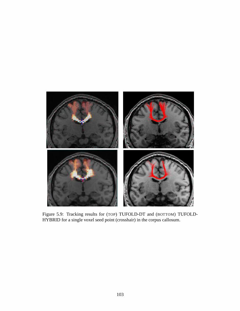
Figure 5.9: Tracking results for (TOP) TUFOLD-DT and (BOTTOM) TUFOLD-HYBRID for a single voxel seed point (crosshair) in the corpus callosum.

103

Figure 5.10: Tracking results for (TOP) TUFOLD-DT and (BOTTOM) TUFOLD-HYBRID for a single voxel seed point (crosshair) near the cortex.

104

The scalar connectivity index assigned in TUFOLD is useful for assessing our

certainty in a reconstructed tract’s existence. However, interpreting the likelihood

values in terms of which tracts do and do not exist is left to the user, and requires a

certain amount of a priori knowledge. For example, we consider the tracking results

shown in Figure 5.10, where the seed point was placed close to the cortex. This is

an area of significant partial volume averaging of fibre directions. TUFOLD-DT

and TUFOLD-HYBRID give slightly different results: TUFOLD-HYBRID recon-

structs a U-fibre with high likelihood, and also reconstructs other lower likelihood

association pathways as well as connections to the contralateral hemisphere via

the corpus callosum. The TUFOLD-DT reconstruction indicates a connection to

the descending cortical spinal tract as well, and does not reconstruct the U-fibre

as well. The failure to reconstruct the U-fibre as well was probably because of a

situation where partial volume averaging of fibre directions lead to ambiguity in

the tensor-described ODF: the reconstruction may have been confounded by flow

of the evolving surface�

in directions that did not correspond to fibres, as is pos-

sible, for example, in cases such as that shown in Figure 3.7. We suggest that the

TUFOLD-HYBRID results are more accurate and that it is probable that the seed

voxel contains fibres from all of the tracts reconstructed by this method. The tensor

model was not as capable of handling the partial volume averaging of directions as

was the q-ball approach. We emphasize, however, that it is up to the user to choose

whether this is the case, or whether the connections shown are the result of the tract

passing through a voxel containing a “bottleneck” of fibres, including fibres from

another fascicles that do not in fact pass through the seed: jumping from tract to

tract can occur in this way.

In summary, both the TUFOLD-DT and TUFOLD-HYBRID approaches yield

tracking results that agree with known human anatomy. The TUFOLD-QB ap-

105

proach appeared to give noisier tract reconstructions, which can be explained by

q-ball being a model-free diffusion ODF reconstruction method, which makes it

more susceptible to noise-induced artifacts than is the highly-constrained tensor

reconstruction method. Where the diffusion tensor fit is good, this noise in the

diffusion ODF is detrimental to the tracking results, however, in cases where the

tensor fit is poor, the high angular resolution ODF obtained with QBI can poten-

tially help control the flow and assign more reasonable likelihood of connection

values. Assessment of which of these methods is superior and in what cases is

difficult without ground truth, therefore further ex-vivo evaluation is necessary to

validate this algorithm.

106

Chapter 6

Flow-based fibre tracking with

diffusion tensor and q-ball data:

validation and comparison to

principal diffusion direction

techniques

6.1 Preface

In Chapter 5, we showed qualitative results in the human brain for the TUFOLD

tracking algorithm using both diffusion tensor and q-ball data. We noted that full

evaluation of hthe algorithm’s performance was difficult without ground truth. In

this chapter, we quantitatively evaluate the performance of TUFOLD with differ-

ent types of input data, and compare it to a well-established principal diffusion

�This chapter is based on a published abstract [30] and a paper that has been submitted to

NeuroImage.

107

direction fibre tracking technique, FACT [115], which we have described in Sec-

tion 2.3.1. The comparison is done with diffusion MRI data acquired using an

anisotropic diffusion phantom with known connectivity, so as to evaluate the track-

ing algorithms in the presence of real imaging artifacts and noise. We describe a

method for quantitatively evaluating the results of tracking algorithms given any

“gold standard” connectivity map. We show the potential of TUFOLD to map con-

nections in regions of subvoxel partial volume averaging of fibre directions, which

can be difficult to map with PDD-based methods. We then show that the fibre track-

ing results can be improved by using high angular resolution reconstruction of the

diffusion orientation distribution function in cases where the diffusion tensor model

fits the data poorly, i.e., the TUFOLD-HYBRID approach. Finally, we qualitatively

compare TUFOLD to FACT in a healthy human brain.

6.2 Introduction

There is significant interest in evaluating the performance and reliability of white

matter fibre tractography algorithms. While simulated data can provide a gold stan-

dard to which tracking results can be compared [94, 103, 177], it is of additional

value to evaluate the results of tracking on real MRI data, in the presence of nor-

mal imaging artifacts, noise characteristics, and voxel size limitations. Doing so

allows us to validate the fibre tracking process from acquisition of the MRI data,

to estimation of the diffusion displacement distribution, to the tracking algorithm

itself.

In this study, we quantitatively compare the performance of TUFOLD to that of

a well-established principal diffusion direction (PDD) algorithm, Fibre Assignment

with Continuous Tracking (FACT) [115]. To do so, we designed a physical phantom

with known connectivity from excised rat spinal cord. Previous validation studies,

108

such as that described in Chapter 4, have been done using the simple case of a single

excised cord [33, 188] and in the macaque [138]: in this study, complex, known

configurations of subvoxel curvature and fibre crossing are created and scanned at

a standard human imaging resolution. These configurations allow us to explore

tracking performance in the presence of subvoxel partial volume averaging of fibre

directions such as that which would be encountered in clinical human studies.

This chapter first focuses on how using the full diffusion tensor instead of the

principal eigenvector only can affect fibre tracking results. Next, it explores how

using HARD data can further affect the tractography. The study was designed to

investigate the advantages and disadvantages of each fibre tracking approach.

6.3 Methods

6.3.1 Tracking algorithm implementation: TUFOLD and FACT

The TUFOLD algorithm was implemented as described in Chapter 5. We required

that the fractional anisotropy be greater than 0.1 and the curvature from voxel to

voxel be less than 80�. We will again refer to TUFOLD run using diffusion ten-

sor data only as TUFOLD-DT, TUFOLD run with q-ball data only will be called

TUFOLD-QB, and the TUFOLD algorithm, run with diffusion tensor data where

the diffusion tensor fit is good, and QBI data elsewhere, will be called TUFOLD-

HYBRID.

For comparison with TUFOLD, the FACT algorithm [115] was implemented us-

ing the same stopping criteria as were used for TUFOLD. For each voxel in the seed

region, we assigned multiple sub-voxel seed points: 27 evenly spaced seed points

were positioned on a grid within the voxel. This allows for branching of tracts from

a single voxel seed region of interest (ROI). From each seed point, the reconstructed

109

tract follows the direction of the principal eigenvector, � � , of the diffusion tensor in

that voxel until it enters another voxel, at which point the direction of propagation

immediately changes to that of � � of the new voxel, and tracking continues until

the stopping criteria occur. Voxels are assigned � � =1 if a reconstructed tract passes

through them and � � =0 if not. In this work, the FACT algorithm was run only with

diffusion tensor data and will be called FACT-DT for clarity.

6.3.2 Anisotropic diffusion phantom experiments

Construction

For evaluation of TUFOLD and comparison to FACT, a physical phantom with

known connectivity was constructed from excised rat spinal cord. The background

for this choice of phantom was discussed in Section 3.2. Phantom construction

and scanning were performed on two separate occasions. On each occasion, two

Sprague-Dawley rats were euthanized and their spinal cords surgically excised.

Phantom #1 was constructed using one year old rats, whose spinal cords measured

approximately 12.5 cm in length and 5 mm in diameter (tracts #1 and #2 in Figure

6.2). Phantom #2 used 4 month old rats, with cords approximately 7 cm long and

5 mm in diameter (tracts #3 and #4 in Figure 6.2). The rats were perfused with

saline for phantom #1 only. The surgeries lasted 1.5 hours each. During the first

surgery, a 500 ml solution of 2% agar was prepared in a 13 cm isotropic polystyrene

container and allowed to cool. During the second surgery, a second 500 ml solution

of 2% agar was prepared. The fresh cords were arranged (see Figure 6.1) on top

of the cooled agar in the container. The two phantoms had similar configurations

of curved, straight, and crossing tracts. The remaining agar was poured over the

cords when it had reached 45�C. It was then left to set and cool. For phantom #1, a

third, fixed cord was added in order to explore the option of using fixed tissue for a

110

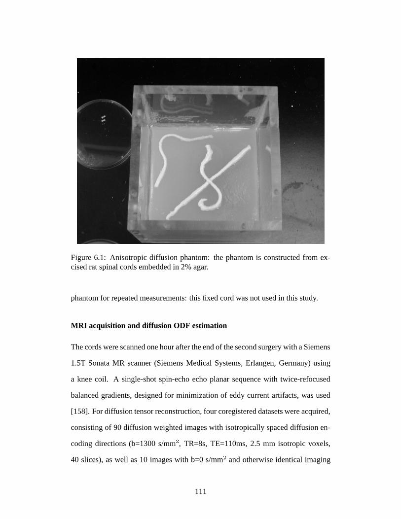
Figure 6.1: Anisotropic diffusion phantom: the phantom is constructed from ex-cised rat spinal cords embedded in 2% agar.

phantom for repeated measurements: this fixed cord was not used in this study.

MRI acquisition and diffusion ODF estimation

The cords were scanned one hour after the end of the second surgery with a Siemens

1.5T Sonata MR scanner (Siemens Medical Systems, Erlangen, Germany) using

a knee coil. A single-shot spin-echo echo planar sequence with twice-refocused

balanced gradients, designed for minimization of eddy current artifacts, was used

[158]. For diffusion tensor reconstruction, four coregistered datasets were acquired,

consisting of 90 diffusion weighted images with isotropically spaced diffusion en-

coding directions (b=1300 s/mm � , TR=8s, TE=110ms, 2.5 mm isotropic voxels,

40 slices), as well as 10 images with b=0 s/mm � and otherwise identical imaging

111

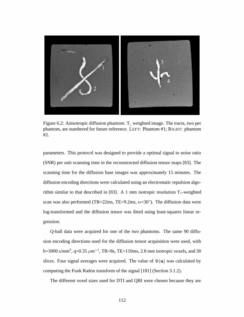
Figure 6.2: Anisotropic diffusion phantom: T � weighted image. The tracts, two perphantom, are numbered for future reference. LEFT: Phantom #1; RIGHT: phantom#2.

parameters. This protocol was designed to provide a optimal signal to noise ratio

(SNR) per unit scanning time in the reconstructed diffusion tensor maps [83]. The

scanning time for the diffusion base images was approximately 15 minutes. The

diffusion encoding directions were calculated using an electrostatic repulsion algo-

rithm similar to that described in [83]. A 1 mm isotropic resolution T � -weighted

scan was also performed (TR=22ms, TE=9.2ms, � =30�). The diffusion data were

log-transformed and the diffusion tensor was fitted using least-squares linear re-

gression.

Q-ball data were acquired for one of the two phantoms. The same 90 diffu-

sion encoding directions used for the diffusion tensor acquisition were used, with

b=3000 s/mm � , q=0.35 � m �� , TR=8s, TE=110ms, 2.8 mm isotropic voxels, and 30

slices. Four signal averages were acquired. The value of( � � � was calculated by

computing the Funk Radon transform of the signal [181] (Section 3.1.2).

The different voxel sizes used for DTI and QBI were chosen because they are

112

representative of voxel sizes used in the literature [81,181], and reflect the inevitable

tradeoff between spatial and angular resolution for any fixed scanning time.

Tractography evaluation

For each phantom, digital gold standard maps (

) of each of the two tracts were

defined.�

is a binary map with a value of one in all voxels identified to lie

on that tract. The gold standard maps were defined by combined automatic and

manual segmentation of the scalar image of the trace of the diffusion tensor, using

a threshold of trace(D) � 1.0E-6 mm � /ms. The trace map was generated from the

average of all measurements of the b=1300 s/mm � , 2.5 mm isotropic voxel size,

dataset. The two tracts crossed in one region, therefore some voxels were identified

to lie in both.

In each gold standard tract, five evenly spaced seed ROIs were defined: these

consisted of one voxel thick cross-sections of the cord. To evaluate the performance

of TUFOLD with q-ball reconstruction, the gold standard and seed ROI maps de-

fined for the 2.5 mm isotropic dataset were resampled using trilinear interpolation

to match the 2.8 mm isotropic dataset.

For evaluation, the � � map for TUFOLD was thresholded in order to create

a binary map equal to one to all voxels with � � above the threshold, and zero to

all voxels with � � below the threshold. For this study, the threshold was that which

produced the lowest error measure, as described below. For each binary � � map, we

calculated an error measure�, given by the sum of the Euclidian distances between

each gold standard voxel and the nearest tracked voxel and the Euclidian distances

between the remaining tracked voxels and the gold standard (this is illustrated in

Figure 6.3).�

was then normalized by dividing by the sum of the distances between

the gold standard

and the seed region. Hence, the error measure is equal to 1

113

Figure 6.3: Schematic of error measure�

used for tract evaluation. The gold stan-dard is shown in black, and the tracking result in dotted orange. The error measureis the sum of the distances between each gold standard voxel and the nearest trackedvoxel (these distances are shown in green) and the distances between the remainingtracked voxels and the gold standard (blue), normalized by dividing by the sum ofthe distances from each gold standard voxel to the seed region.

if the tracking goes nowhere, and is zero in the case of perfect tracking. The error

measure penalizes both going off track (“false positives”) and incomplete tracking

(“false negatives”).

The TUFOLD-DT and FACT-DT algorithms were evaluated for the following

datasets: (i) diffusion tensor reconstruction of the 90 diffusion encoding direction

acquisition, b=1300 s/mm � (for which we have 4 separate datasets consisting of one

signal average each); (ii) diffusion tensor reconstruction of a subset of 30 of the 90

diffusion encoding directions used in (i); (iii) diffusion tensor reconstruction of 2,

3, and 4 averages of the four 90 diffusion encoding direction acquisitions, b=1300

s/mm � ; and (iv) diffusion tensor reconstruction of the average of the four 90 dif-

fusion encoding direction acquisitions with b=3000 s/mm � . (ii)-(iv) were done for

phantom #1 only. TUFOLD-QB and TUFOLD-HYBRID were then evaluated us-

ing the average of the four 90 diffusion encoding direction acquisitions with b=3000

s/mm � . The region� � � � �� consisted of the crossing region, most of the

curved parts of tract #2, and some parts of the straight tract #1. The high � � in

114

some parts of the straight cord was most likely due to partial volume averaging of

nerve roots, which branch from the cord, with the spinal column. For all tracking

experiments, the data were first supersampled to half the original voxel size in each

dimension using trilinear interpolation.

6.3.3 Human brain experiments

Human brain tractography was performed with data acquired from one healthy

subject using the same imaging protocol given above for both diffusion tensor

and q-ball reconstruction. One signal average was acquired for both the b=1300

s/mm � and b=3000 s/mm � acquisitions. An eight-channel phased-array head coil

equipped with a custom immobilization device was used instead of a knee coil (as

was the case for the phantom). The b=1300 s/mm � and b=3000 s/mm � datasets

were acquired in separate sessions and were subsequently registered using semi-

automatic techniques [49]. Informed consent was obtained prior to participation

in the study. Tracking was performed with TUFOLD and FACT, and the track-

ing results from each algorithm were compared to each other and to known human

anatomy. Both the FACT-DT and TUFOLD-DT tracking were performed with the

optimized b=1300 s/mm � acquisition, while TUFOLD-HYBRID tracking was per-

formed using the b=3000 s/mm � acquisition.

6.4 Results

6.4.1 Performance of TUFOLD versus that of FACT

In our first experiments, we compared the performance of TUFOLD using the ten-

sor ODF (the ODF is shown in figures 6.4c and 6.4d) to the performance of FACT

using the principal eigenvector of the diffusion tensor (Figure 6.4b). These re-

115

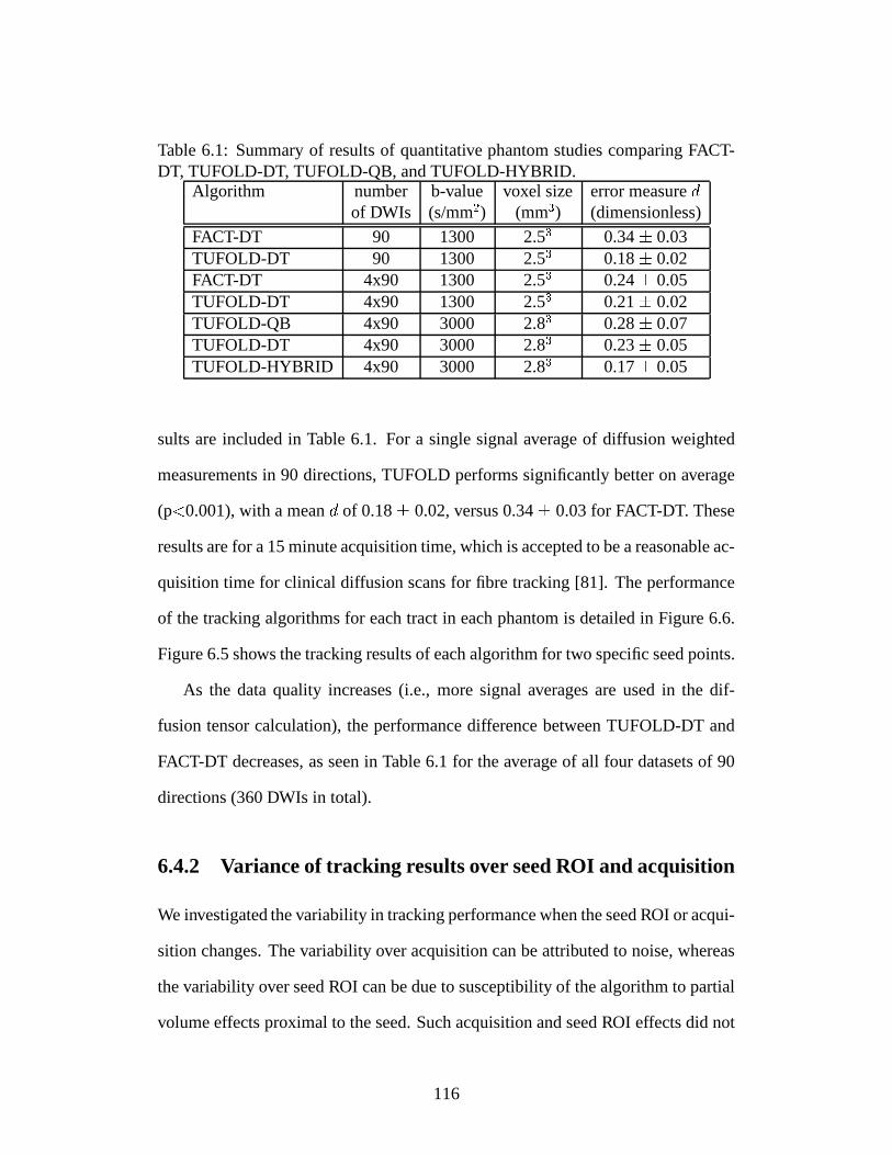
Table 6.1: Summary of results of quantitative phantom studies comparing FACT-DT, TUFOLD-DT, TUFOLD-QB, and TUFOLD-HYBRID.

Algorithm number b-value voxel size error measure�

of DWIs (s/mm � ) (mm ) (dimensionless)

FACT-DT 90 1300 2.5 0.34 � 0.03TUFOLD-DT 90 1300 2.5 0.18 � 0.02FACT-DT 4x90 1300 2.5 0.24 � 0.05TUFOLD-DT 4x90 1300 2.5 0.21 � 0.02TUFOLD-QB 4x90 3000 2.8 0.28 � 0.07TUFOLD-DT 4x90 3000 2.8 0.23 � 0.05TUFOLD-HYBRID 4x90 3000 2.8 0.17 � 0.05

sults are included in Table 6.1. For a single signal average of diffusion weighted

measurements in 90 directions, TUFOLD performs significantly better on average

(p � 0.001), with a mean�

of 0.18 � 0.02, versus 0.34 � 0.03 for FACT-DT. These

results are for a 15 minute acquisition time, which is accepted to be a reasonable ac-

quisition time for clinical diffusion scans for fibre tracking [81]. The performance

of the tracking algorithms for each tract in each phantom is detailed in Figure 6.6.

Figure 6.5 shows the tracking results of each algorithm for two specific seed points.

As the data quality increases (i.e., more signal averages are used in the dif-

fusion tensor calculation), the performance difference between TUFOLD-DT and

FACT-DT decreases, as seen in Table 6.1 for the average of all four datasets of 90

directions (360 DWIs in total).

6.4.2 Variance of tracking results over seed ROI and acquisition

We investigated the variability in tracking performance when the seed ROI or acqui-

sition changes. The variability over acquisition can be attributed to noise, whereas

the variability over seed ROI can be due to susceptibility of the algorithm to partial

volume effects proximal to the seed. Such acquisition and seed ROI effects did not

116

a b

c d

e f

Figure 6.4: Evidence of subvoxel partial volume averaging of fibre directions in theanisotropic diffusion phantom. (a) Crossing region. (b) Preferred direction of diffu-sion as given by the principal eigenvector of the diffusion tensor. Vectors are shownonly within the gold standard map. (c) DTI reconstruction of the diffusion ODF. (d)Zoom of central region. (e) QBI reconstruction from the same diffusion weightedimages. (f) Zoom of central region. There is support for a fibre running through thecrossing region from bottom left to top right in the QBI data, but streamline track-ing using the principal eigenvector can easily be confounded by the presence of aperpendicular fibre. The DTI shapes in this region are pancake-like, so flow in alldirections above the mean of the ODF will result in both tracts being reconstructed.

117

a b c

Figure 6.5: Surface rendering of connected voxels: (a) Voxels identified as goldstandard voxels: tract #1 (red) and tract #2 (green). Voxels reached using (b) FACT-DT and (c) TUFOLD-DT with seeding in each of the two tracts.

FACT−DT TUFOLD−DT0

0.1

0.2

0.3

0.4

0.5

perf

orm

ance

mea

sure

d (

unitl

ess)

tract 1tract 2tract 3tract 4all tracts

Figure 6.6: Results: FACT-DT vs TUFOLD-DT: 90 DWI acquisition. The errormeasures for all four tracts are shown, as well as the average error measure for thefour tracts.

118

appear to be correlated across algorithms, indicating that the two algorithms have

different dependencies on noise and partial volume effects.

We calculated the magnitude of the variability over acquisition and seed ROI

for the two algorithms. The standard deviation of�

over acquisition was calculated

for all (seed,tract) pairs for each algorithm to give a measure of the variability over

acquisition, giving an average standard deviation of " � � � =0.15 � 0.06 for FACT-

DT (overall mean�

of 0.38) and " � � � =0.10 � 0.09 for TUFOLD-DT (overall mean�

of 0.17). Both values are 30-50% of the mean score.

The standard deviation of�

was calculated for all (acquisition,tract) pairs for

each algorithm to give a measure of the seed point dependence. The average stan-

dard deviation over seed point was " � � � =0.14 � 0.05 for FACT-DT and " � � � =0.09

� 0.07 for TUFOLD-DT. This variability was comparable to the variability over

acquisition: the two effects appear to have equivalent magnitudes.

6.4.3 Dependence of performance on noise level

As shown in Table 6.1, as the signal to noise ratio of the data increased, the per-

formance difference between TUFOLD-DT and FACT-DT decreased. We looked

at this relationship in more detail by computing the average error measure for two,

three, and four averages of the 90 direction diffusion weighting scheme, as well as

a subset of 30 directions from one dataset. The results are shown in Figure 6.7 and

are tabulated in Table 6.1, where the total number of DWIs is the number of signal

averages times the number of diffusion encoding directions.

6.4.4 TUFOLD: DTI reconstruction versus QBI reconstruction

The diffusion ODF calculated using q-ball reconstruction is shown in Figures 6.4e

and 6.4f. These data were used to compare TUFOLD-QB to TUFOLD-DT using

119

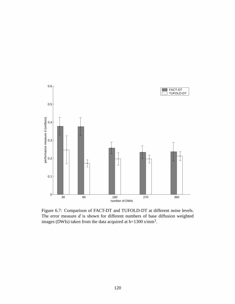
30 90 180 270 3600

0. 1

0. 2

0. 3

0. 4

0. 5

0. 6

number of DWI s

performance measure d (unitless)

FACT-DTTUFOLD-DT

Figure 6.7: Comparison of FACT-DT and TUFOLD-DT at different noise levels.The error measure

�is shown for different numbers of base diffusion weighted

images (DWIs) taken from the data acquired at b=1300 s/mm � .

120

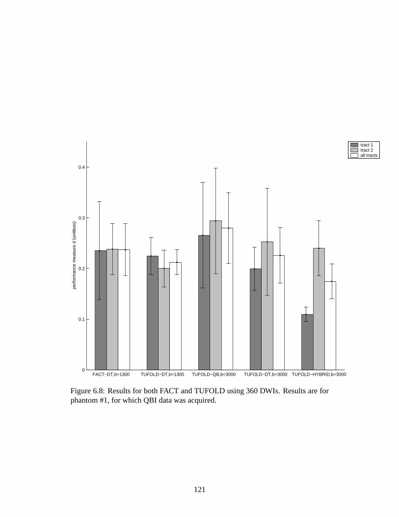
FACT−DT,b=1300 TUFOLD−DT,b=1300 TUFOLD−QB,b=3000 TUFOLD−DT,b=3000 TUFOLD−HYBRID,b=30000

0.1

0.2

0.3

0.4

perf

orm

ance

mea

sure

d (

unitl

ess)

tract 1tract 2all tracts

Figure 6.8: Results for both FACT and TUFOLD using 360 DWIs. Results are forphantom #1, for which QBI data was acquired.

121

a b c d

Figure 6.9: Surface rendering of connected voxels: (a) Voxels identified as goldstandard voxels: tract #1 (red) and tract #2 (green). Voxels reached using (b)TUFOLD-DT, (c) TUFOLD-QB, and (d) TUFOLD-HYBRID with seeding in eachof the two tracts.

the tensor ODF computed using an equivalent number of diffusion encoding direc-

tions and an optimized b-value of b=1300 s/mm � . The TUFOLD-QB approach had

poorer results (Figure 6.8 and Table 6.1), with�=0.28 � 0.07. To determine whether

the difference was due to the acquisition parameters or to the ODF reconstruction,

we did tracking with TUFOLD using the tensor reconstruction of the b=3000 s/mm �

data. DT reconstruction of these data performed as well as DT reconstruction of the

b=1300 data s/mm � (Figure 6.8 and Table 6.1).

Next, TUFOLD-HYBRID tracking was performed using the b=3000 data s/mm �

diffusion weighted data. The error measures (Figure 6.8 and Table 6.1) suggest a

trend toward better performance with the hybrid approach, which has a lower mean�

(0.17 � 0.05) than either the q-ball or tensor reconstruction alone. Figure 6.9

shows the best tracking results obtained with TUFOLD-DT, TUFOLD-QB, and

TUFOLD-HYBRID using four signal averages of 90 diffusion encoding directions.

122

a b c

Figure 6.10: Tracking results: TOP: Maximum intensity projection (MIP) of like-lihood of connection map. BOTTOM: User-thresholded tracts projected on a 2Dplane. (a) TUFOLD-DT, (b) TUFOLD-HYBRID with threshold of

� � � � � � � � �� ,and (c) FACT-DT: the likelihood of connection ( � � ) map in the case of FACT-DTis binary. The single-voxel seed point (crosshair) was placed in the splenium of thecorpus callosum. For TUFOLD, the � � maps are windowed to show the most likelyconnections: there are non-zero � � values elsewhere.

6.4.5 Human brain experiments

Figures 6.10-6.12 show fibre tracking results in the human brain for FACT-DT,

TUFOLD-DT, and TUFOLD-HYBRID. These figures illustrate tracking in major

commissural fibre tracts (Figures 5.8 and 5.9) and more subtle sub-cortical path-

ways (Figure 5.10). They are meant to illustrate the advantages and disadvantages

of tracking using the principal eigenvector only, the full diffusion tensor, and q-ball

reconstruction, respectively.

123

a b c

Figure 6.11: Tracking results for (a) TUFOLD-DT, (b) TUFOLD-HYBRID, and(c) FACT-DT for a single voxel seed point (crosshair) in the corpus callosum.

a b c

Figure 6.12: Tracking results for (a) TUFOLD-DT, (b) TUFOLD-HYBRID, and(c) FACT-DT for a single voxel seed point (crosshair) near the cortex.

124

6.5 Discussion

We have shown that a flow-based fibre tracking algorithm, TUFOLD, which allows

for tract propagation in multiple directions, can improve fibre tracking results in the

presence of partial volume averaging of fibre directions. Using QBI data instead

of DTI data in cases where the tensor fit is poor can further improve the tracking

results.

In the case of partial volume averaging of fibre directions which we created in

our phantom, many of the tracts propagated using the FACT-DT algorithm did not

pass through the crossing region (see Figure 6.5b), probably because the principal

eigenvector direction did not lie along the tract direction. Additionally, the tracts

that did pass through the crossing region stopped before reaching the ends of the

cord because noise and/or imaging artifacts caused the principal eigenvector direc-

tion to be slightly deflected, hence leading the path out of the cord. TUFOLD-DT

was better able to overcome these issues: most of the errors in the TUFOLD-DT

tracking were due to bleeding down the perpendicular tract, despite the curvature

constraint, as can be seen in Figure 6.5c. This is a large region of crossing, and

reconstructed tracts can therefore turn slowly from one tract to another without ex-

ceeding the curvature constraint. Such scenarios can often occur with typical voxel

sizes in vivo. With the tensor approach, the disc-like ODF makes it difficult to con-

trol the flow in these cases. However, the use of q-ball data in the crossing region

improved the results, which suggests that the multi-peaked ODFs in this region (see

Figures 6.4e and 6.4f) caused the flow to be fast only along the tract directions, as

opposed to flowing at comparable speeds in all directions in the plane of the cross-

ing, as would occur with the tensor approach. In the QBI case, if the flow bends

down the wrong tract, it is more likely to be stopped by the curvature constraint. In

further work, we propose to use a relaxation labeling scheme such as that in [78] in

125

order to better distinguish large scale crossing from branching, which would facili-

tate the use of a stricter curvature constraint in cases of crossing.

We note that using q-ball data only, as done in the TUFOLD-QB approach, per-

formed less well than did TUFOLD-DT using the same base diffusion weighted im-

ages, which performed comparably to TUFOLD-DT using base diffusion weighted

images with lower b-values. The poor performance of TUFOLD-QB therefore was

not attributed to the lower SNR of the base DWIs, the larger voxel size, or the in-

creased eddy current induced artifacts due to higher slew rates, but rather to the

QBI reconstruction itself. Using the q-ball ODF when the tensor fit is good only

increases susceptibility to noise, however, when the tensor fit is poor, the high an-

gular resolution ODF obtained with QBI can help control the flow and assign more

reasonable likelihood of connection values.

In the human brain experiments, FACT-DT showed a tendency to jump incor-

rectly from one tract system to another: in Figure 6.10c, FACT-DT reconstructs a

false connection to a visual pathway from V1, while in Figure 6.12c, the FACT-

DT tracking was confounded by the large fibres of the pyramidal tract, and turned

incorrectly down through the internal capsule. The voxels reached by these connec-

tions had very low likelihood of connection values in both the TUFOLD-DT and

TUFOLD-HYBRID approaches: this is a case where assigning a non-binary likeli-

hood of connection can help identify uncertain pathways that are reconstructed due

to partial volume averaging of fibre directions, or to noise. We note that we could

assign the same likelihood measure to the tracts reconstructed with FACT-DT prop-

agation: we propagate only along the principal diffusion direction (the maximum

of the tensor-described diffusion ODF(

), note the magnitude of(

in this direc-

tion, and define the minimum along the tract of this value to be the tract likelihood.

While this approach could help narrow down which of the tracts that are recon-

126

structed have high likelihood of existence, it would fail whenever a connection is

not reconstructed with the PDD approach, for example, in the case of ‘flat’ tensors,

where the principal diffusion direction may not coincide with the tract direction.

Using the full tensor, as in the TUFOLD-DT approach, can deal with these prob-

lems to an extent, however, in cases where the maximum of the tensor-described

ODF is incorrect (e.g., the nonorthogonal crossings shown in Figure 3.7), the use

of q-ball data should be more accurate.

Imaging noise can cause tracking to stop or proceed down the wrong path in ei-

ther algorithm. The results suggest that TUFOLD is more robust in the presence of

noise. Hence, when tracking using datasets acquired with low SNR, either because

of small voxel sizes, short acquisition times, or significant partial volume averaging

of fibres with isotropic material, TUFOLD is superior. However, the two algorithms

plateau at the same performance level at higher SNR, meaning the advantages and

disadvantages are balanced for the two algorithms at this point. The choice of which

algorithm to use depends on the type of fibre structure expected in any fibre track-

ing application: for example, if many subvoxel crossings are expected, TUFOLD

should be superior.

While an optimized scheme was used for the tensor acquisition, the QBI pro-

tocol has not been optimized. A theoretical framework for determining the ideal

b value for achieving high angular resolution, given that SNR decreases as b in-

creases, has not been outlined. The range in the number of diffusion weighted

measurements from N=90 (used here) to N=492 (used by Tuch et al. [181]) has not

been explored. Further investigation is also necessary to determine the optimal bal-

ance between angular resolution and spatial resolution for any given scanning time.

The ideal protocol for diffusion measurements for the purpose of fibre tracking will

depend on the time the subject can comfortably stay in the MR scanner, and the size

127

and complexity of the fibre structures being studied.

This study showed a high variability in the tracking performance over seed ROI

in the phantom, as discussed in Section 6.4.2. It is fair to suggest that if we start

tracking iteratively from all voxels in the volume (the “brute force” approach), and

ask from which starting voxels the seed ROI is reached, and with what likelihood,

we will get a different answer from the outward propagation approach. However,

the tracking performance when starting from the seed ROI only should correlate

with the performance when tracking is initiated everywhere, and takes significantly

less computation time. This study was meant to give results from the forward track-

ing approach only, and should be indicative of how reliable other approaches would

be.

In summary, our findings suggest that using the full diffusion tensor for fibre

tracking, using methods such as TUFOLD, can provide superior results to ap-

proaches using only the principal direction of diffusion. Furthermore, HARD re-

construction of the diffusion ODF, illustrated here using the q-ball reconstruction

method, can further improve the results when used in voxels in which the tensor

model fits the data poorly. We have done extensive validation with a gold standard

tract configuration. Tracking with all algorithms is confounded by noise, partial

volume averaging of fibre directions, large voxels in the base diffusion weighted

images, and limitations of the diffusion pdf measurement. Of the methods consid-

ered here, TUFOLD-HYBRID appears most robust to these confounds.

128

Chapter 7

Discussion and conclusions

7.1 Summary of results

This thesis has described the development of two geometric flows for reconstructing

white matter fibre tracts in the central nervous system using diffusion MRI. In do-

ing so, the underlying physics and assumptions inherent in diffusion tensor and high

angular diffusion imaging have been described. The first algorithm was conceived

as a preliminary step and used only the information in the principal eigenvector of

the diffusion tensor. The second algorithm, which we have named Tracking Using

Fibre Orientation Likelihood Distribution (TUFOLD), overcomes many of the lim-

itations of the first approach. It lends itself easily to be used with either diffusion

tensor or high angular resolution diffusion data, and was demonstrated using both

methods. Specifically, a hybrid approach using the diffusion tensor method of re-

constructing the diffusion orientation function when the diffusion tensor model fit

the data well and the q-ball method of reconstructing of the diffusion ODF when

the diffusion tensor fit was poor was implemented. The q-ball acquisition protocol

was designed to resolve multiple subvoxel fibre directions in all voxels of the brain

in a clinically feasible time frame.

129

The TUFOLD fibre tracking algorithm performance was demonstrated both in

vivo and in a physical phantom designed to have anisotropic diffusion properties

and fibre connections with complex configurations similar to those encountered in

the human brain. TUFOLD, using the tensor-described diffusion ODF, was com-

pared to a well established principal diffusion direction streamline fibre tracking

algorithm, FACT [115]. It showed superior performance when the underlying dif-

fusion data had a lower signal to noise ratio, and in areas of subvoxel partial vol-

ume averaging of fibre directions. The performance of the TUFOLD algorithm

using the hybrid approach was compared to that using diffusion tensor data only,

and the results suggested that using q-ball reconstruction when there was evidence

of subvoxel partial volume averaging of fibre directions could further improve the

tracking results. However, we note that the q-ball reconstruction method is more

sensitive to noise than is the tensor method, and the decision to use one method over

the other should be made after considering the properties of the fibre structures to

be investigated and the quality of the data available.

7.2 Conclusions

In conclusion, our findings suggest that methods such as TUFOLD, by virtue of us-

ing the full two-dimensional diffusion orientation distribution function as input, can

be more robust to noise and partial volume effects than are fibre tracking methods

using only the principal eigenvector of the diffusion tensor. Furthermore, HARD

reconstruction of the diffusion ODF, illustrated here using the q-ball reconstruction

method, can further improve the results when used in voxels in which the tensor

model fits the data poorly. However, HARD reconstruction methods suffer from in-

creased processing time, lower SNR, and susceptibility to noise, so should be used

only when the benefits of resolving multiple subvoxel fibre directions are expected

130

to outweigh these drawbacks.

7.3 Issues in fibre tracking using diffusion MRI: fu-

ture work

The field of diffusion MRI can expect to see more developments in the near fu-

ture. The high angular resolution diffusion techniques described in this thesis are

relatively new compared to the tensor approach, and will benefit from further re-

finement and optimization. Agreement has not yet been reached on the tradeoff

between spatial and angular resolution with such techniques. New algorithms for

the measurement of the HARD ODF may be developed. While many regulariza-

tion techniques exist for diffusion tensor data, regularization of non-analytic HARD

data many be possible using relaxation labeling or anisotropic diffusion smoothing.

Additionally, the estimation of the fibre orientation likelihood distribution function

from the diffusion ODF is an area of active research [178].

Fibre tracking algorithms can still be improved. Many existing fibre tracking

approaches could benefit from a robust algorithm to distinguish large scale fibre

crossing from branching or bottlenecks. This was a case that was seen to be con-

founding even in TUFOLD: certainty as to whether a region is a crossing or not

would greatly reduce uncertainty in tracking results. The use of fibre tractogra-

phy in the numerous clinical applications in which it has potential will give further

insight into how algorithms need to be improved.

Diffusion MRI is very sensitive to subject motion and other imaging artifacts,

and robust motion correction and artifact reduction are still an area of research ac-

tivity. Due to its inherently low SNR, diffusion MRI is performed at relatively low

spatial resolution compared to standard anatomical imaging protocols. Improved

131

scanner hardware, including higher field magnets, will help improve the resolution.

Further hardware and software improvements may help make even higher resolu-

tion feasible in clinical time frames. We propose that in addition to pursuing high

resolution single-acquisition protocols, multi-session scans be performed in order

to obtain a very high resolution reference diffusion data set for use in basic neu-

roanatomic research.

132

Appendix A

Ethics approval for human studies

The human studies included in this thesis were approved by the Montreal Neuro-

logical Institute and Hospital Research Ethics Board. The following document is

the confirmation of approval.

133

Bibliography

[1] A. Abragam. Principles of Nuclear Magnetism. Oxford University Press,

New York, 1961.

[2] C.B. Ahn and Z.H. Cho. Analysis of eddy currents in nuclear magnetic

resonance imaging. Magnetic Resonance in Medicine, 17:149–163, 1991.

[3] E. T. Ahrens, D. H. Laidlaw, C. Readhead, C. F. Brosnan, S. E. Fraser, and

R. E. Jacobs. MR microscopy of transgenic mice that spontaneously acquire

experimental allergic encephalomyelitis. Magn Reson Med, 40(1):119–32.,

Jul 1998.

[4] A. Aldroubi and P. Basser. Reconstruction of vector and tensor fields from

sampled discrete data. Contemporary Mathematics, 247:1–15, 1999.

[5] A.L. Alexander, K.M. Hasan, M. Lazar, J.S. Tsuruda, and Parker D.L. Anal-

ysis of partial volume effects in diffusion-tensor MRI. Magn Reson Med,

45(4):770–780, 2001.

[6] A.L. Alexander, J.S. Tsuruda, and D.L. Parker. Elimination of eddy current

artifacts in diffusion-weighted echo-planar images: the use of bipolar gradi-

ents. Magnetic Resonance in Medicine, 38:1016–1021, 1997.

135

[7] D.C. Alexander, G.J. Barker, and S.R. Arridge. Detection and modeling

of non-Gaussian apparent diffusion coefficient profiles in human brain data.

Magnetic Resonance in Medicine, 48:331–340, 2002.

[8] D.C. Alexander and K.M. Jansons. Spin echo attenuation to diffusion den-

sity: a general inversion for measurements on a sphere. In International

Society for Magnetic Resonance in Medicine Workshop on Diffusion MRI:

Biophysical Issues (What can we measure?), pages 206–209, 2002.

[9] L. Alvarez, J. Weickert, and J. Sanchez. Reliable estimation of dense opti-

cal flow fields with large displacements. International Journal of Computer

Vision, 2001.

[10] A. W. Anderson and J. C. Gore. Analysis and correction of motion artifacts

in diffusion weighted imaging. Magn Reson Med, 32(3):379–87., Sep 1994.

[11] Y. Assaf and P.J. Basser. Combining DT and q-space MRI: A new model

of white matter in the brain. In Proceedings of the International Society for



page 588, 2003.

[12] Y. Assaf, A. Mayk, and Y. Cohen. Displacement imaging of spinal cord

using q-space diffusion-weighted MRI. Magnetic Resonance in Medicine,

44:713–722, 2000.

[13] Atamai Surgical Planning. www.atamai.com.

[14] P. J. Basser. Relationships between diffusion tensor and q-space MRI. Magn

Reson Med, 47(2):392–7., Feb 2002.

136

[15] P.J. Basser, J. Mattiello, and D. Le Bihan. Estimation of the effective self-

diffusion tensor from the NMR spin echo. Journal of Magnetic Resonance,

103:247–254, 1994.

[16] P.J. Basser, S. Pajevic, C. Pierpaoli, J. Duda, and A. Aldroubi. In vivo fiber

tractography using DT-MRI data. Magnetic Resonance in Medicine, 44:625–

632, 2000.

[17] P. Batchelor, D.L.G. Hill, D. Atkinson, F. Calamante, and A. Connelly. Fibre-

tracking by solving the diffusion-convection equation. In Proceedings of the

International Society for Magnetic Resonance in Medicine: 10 ��

Scientific

Meeting and Exhibition, page 1135, 2002.

[18] P.G. Batchelor, D.L.G. Hill, F. Calamante, and D. Atkinson. Study of con-

nectivity in the brain using the full diffusion tensor from MRI. In M.F. Insana

and R.M. Leahy, editors, IPMI 2001, LNCS 2082, pages 121–133, 2001.

[19] C. Beaulieu. The basis of anisotropic water diffusion in the nervous system.

NMR in Biomedicine, 15:435–455, 2002.

[20] T. E. Behrens, M. W. Woolrich, M. Jenkinson, H. Johansen-Berg, R. G.

Nunes, S. Clare, P. M. Matthews, J. M. Brady, and S. M. Smith. Character-

ization and propagation of uncertainty in diffusion-weighted MR imaging.

Magn Reson Med, 50(5):1077–88., Nov 2003.

[21] M Bjornemo, A Brun, R Kikinis, and C.-F. Westin. Regularized stochas-

tic white matter tractography using diffusion tensor MRI. In T. Dohi and

R. Kikinis, editors, MICCAI 2002, LNCS 2488, pages 435–442, 2002.

[22] F. Bloch. Nuclear induction. Physical Review, 70:460–473, 1946.

137

[23] R. Blyth, P. Cook, and D. Alexander. Tractography with multiple fibre direc-

tions. In Proceedings of the International Society for Magnetic Resonance

in Medicine: 11 ��

Scientific Meeting and Exhibition, page 240, 2003.

[24] G. Borgefors. Distance transformations in arbitrary dimensions. CVGIP,

27(3):321–345, September 1984.

[25] S. Bouix, K. Siddiqi, and A. Tannenbaum. Flux driven fly throughs. In Pro-

ceedings of the International Conference On Computer Vision and Pattern

Recognition, Madison, Wisconsin, June 2003.

[26] M.J. Bronskill and P. Sprawls, editors. American Association of Physicists

in Medicine (AAPM) Summer School Proceedings, 1992.

[27] M.A. Brown and R.C. Semelka. MRI: basic physical principles and appli-

cations. Wiley-Liss, 1995.

[28] Robert Brown. A brief account of microscopical observations made in the

months of June, July, and August 1827 on the particles contained in the

pollen of plants; and on the general existence of active molecules in organic

and inorganic bodies. Philosoph. Mag., 4:161, 1828.

[29] F. Calamante, D.A. Porter, D.G. Gadian, and A. Connelly. Magnetic Reso-

nance in Medicine, 41:95–102, 1999.

[30] J.S.W. Campbell, V. Rymar, A.F. Sadikot, K. Siddiqi, and G.B. Pike. Com-

parison of flow- and streamline-based fibre tracking algorithms using an

anisotropic diffusion phantom. In Proceedings of the International Society

for Magnetic Resonance in Medicine: 12 ��

Scientific Meeting and Exhibi-

tion, page 1277, 2004.

138

[31] J.S.W. Campbell, K. Siddiqi, and G.B. Pike. White matter fibre tract likeli-

hood evaluated using normalized RMS diffusion distance. In Proceedings of


Scien-

tific Meeting and Exhibition, page 1130, 2002.

[32] J.S.W. Campbell, K. Siddiqi, and G.B. Pike. Full-brain q-ball imaging in

a clinically acceptable time: Application to white matter fibre tractogra-

phy. In Proceedings of the International Society for Magnetic Resonance

in Medicine: 12 ��


[33] J.S.W. Campbell, K. Siddiqi, B.C. Vemuri, and G.B. Pike. A geometric flow

for white matter fibre tract reconstruction. In Billene Mercer, editor, 2002

IEEE International Symposium on Biomedical Imaging Conference Proceed-

ings, pages 505–508. The Institute of Electrical and Electronics Engineers,

Inc., Omni Press, 2002.

[34] Z. Caramanos, J.S.W. Campbell, S. Narayanan, S. Francis, S. Antel,

H. Reddy, P. Matthews, D.-L. Sappey-Marinier, G.B. Pike, and D. Arnold.

Axonal integrity and fractional anisotropy in the normal-appearing white

matter of patients with multiple sclerosis: Relationship to cerebro-functional

reorganization and clinical disability. In Proceedings of the International

Society for Magnetic Resonance in Medicine: 10 ��

Scientific Meeting and

Exhibition, page 590, 2002.

[35] M.B. Carpenter. Core Text of Neuroanatomy. Williams & Wilkins, Philadel-

phia, 4th edition, 1991.

[36] M.B. Carpenter. The Human Brain. Springer, 2 edition, 1999.

139

[37] H.Y. Carr and E.M. Purcell. Effects of diffusion on free precession in nuclear

magnetic resonance experiments. Physical Review, 94:630, 1954.

[38] V. Caselles, F. Catte, T. Coll, and F. Dibos. A geometric model for active

contours in image processing. Numerische Mathematik, 66:1–31, 1993.

[39] V. Caselles, R. Kimmel, and G. Sapiro. Geodesic active contours. In

ICCV’95, pages 694–699, 1995.

[40] M. Catani, R. J. Howard, S. Pajevic, and D. K. Jones. Virtual in vivo inter-

active dissection of white matter fasciculi in the human brain. NeuroImage,

17(1):77–94., Sep 2002.

[41] M. Catani, D. K. Jones, R. Donato, and D. H. Ffytche. Occipito-temporal

connections in the human brain. Brain, 126(Pt 9):2093–107. Epub, Sep 2003.

[42] T.F. Chan and J. Shen. Variational restoration of non-flat image features:

model and algorithm. SIAM Journal of Applied Mathematics, 61:1338–1361,

2000.

[43] C. Chefd’hotel, D. Tschumperle, R. Deriche, and O. Faugeras. Constrained

flows of matrix-valued functions : Application to diffusion tensor regulariza-

tion. In Proc. 7th ECCV, Copenhaguen, May 2002.

[44] A. Chorin, editor. Computational fluid mechanics, selected papers. Aca-

demic Press, 1989.

[45] O. Ciccarelli, A.T. Toosy, G.J.M. Parker, C.A.M. Wheeler-Kingshott, G.J.

Barker, D.H. Miller, and A.J. Thompson. Diffusion tractography based group

mapping of major white-matter pathways in the human brain. NeuroImage,

19:1545–1555, 2003.

140

[46] C.A. Clark, M. Hedehus, and M.A. Moseley. In vivo mapping of the fast

and slow diffusion tensors in human brain. Magnetic resonance in Medicine,

47:623–628, 2002.

[47] G. G. Cleveland, D. C. Chang, C. F. Hazlewood, and H. E. Rorschach. Nu-

clear magnetic resonance measurement of skeletal muscle: anisotrophy of

the diffusion coefficient of the intracellular water. Biophys J, 16(9):1043–

53., Sep 1976.

[48] Y. Cointepas, C. Poupon, D. Le Bihan, and J.-F. Mangin. A spin glass frame-

work to untangle fiber crossing in MR diffusion based tracking. In T. Dohi

and R. Kikinis, editors, MICCAI 2002, LNCS 2488, pages 475–482, 2002.

[49] D.L. Collins, P. Neelin, T.M. Peters, and A.C. Evans. Automatic 3D inter-

subject registration of MR volumetric data in standardized Talairach space.

Journal of Computer Assisted Tomography, 18(2):192–205, 1994.

[50] T. E. Conturo, R. C. McKinstry, E. Akbudak, and B. H. Robinson. Encoding

of anisotropic diffusion with tetrahedral gradients: a general mathematical

diffusion formalism and experimental results. Magn Reson Med, 35(3):399–

412., Mar 1996.

[51] T.E. Conturo, N.F. Lori, T.S. Cull, E. Akbudak, A. Snyder, L.S. Shimony,

R.C. McKinstry, H. Burton, and Raichle M.E. Tracking neuronal fibre path-

ways in the living human brain. Proceedings of the National Academy of

Science (Neurobiology, Applied Physical Sciences), 96:10422–10427, 1999.

[52] O. Coulon, D.C. Alexander, and S.R. Arridge. A regularization scheme for

diffusion tensor magnetic resonance images. In M.F. Insana and R.M. Leahy,

editors, IPMI 2001, LNCS 2082, pages 92–105, 2001.

141

[53] A. Darquie, J.B. Poline, H. Saint-Jalmes, and D. Le Bihan. Transient de-

crease in water diffusion observed in human occipital cortex during visual

stimulation. In Proceedings of the International Society for Magnetic Reso-

nance in Medicine: 9 ��


[54] Z. Ding, J.C. Gore, and A.W. Anderson. Classification and quantification of

neuronal fiber pathways using diffusion tensor MRI. Magnetic Resonance in

Medicine, 49:716–721, 2003.

[55] D.C. Douglass and D.W. McCall. Diffusion in paraffin hydrocarbins. Journal

of Physical Chemistry, 60:1102, 1958.

[56] R. Duda and P. Hart. Pattern Recognition and Scene Analysis. Wiley, 1973.

[57] P.A. Egelstaff. An introduction to the liquid state. Oxford Science Publica-

tions, Oxford Clarendon Press, 1992.

[58] A. Einstein. Die von der molekularkinetischen theorie der warme geforderte

bewegung von in ruhenden flussigkeiten suspendierten teilchen. Ann Der

Physik, 17:459, 1905.

[59] A. Fick. On liquid diffusion. Philos. Mag., 10:30–39, 1855.

[60] L. R. Frank. Characterization of anisotropy in high angular resolution

diffusion-weighted mri. Magn Reson Med, 47(6):1083–99., Jun 2002.

[61] L.R. Frank. Anisotropy in high angular resolution diffusion-weighted MRI.

Magnetic Resonance in Medicine, 45(6):935–939, 2001.

[62] K. Fredericksen, Amodei. L., W.E. Kaufmann, P.C.M. van Zijl, G.D. Paerl-

son, and S. Mori. Automated white matter delineation tools based on diffu-

sion tensor imaging. In Proceedings of the International Society for Mag-

142


Scientific Meeting and Exhibition, page

1532, 2001.

[63] P. Funk. Uber eine geometrische anwendung der abelschen integralgleich-

nung. Math. Ann., 77:129–135, 1916.

[64] O.A. Glenn, R.G. Henry, J.I. Berman, P.C. Chang, S.P. Miller, D.B. Vi-

gneron, and A.J. Barkovich. DTI-based three-dimensional tractography de-

tects differences in the pyramidal tracts of infants and children with con-

genital hemiparesis. Journal of Magnetic Resonance Imaging, 18:641–648,

2003.

[65] P. Godement, J. Vanselow, S. Thanos, and F. Bonhoeffer. A study in de-

veloping visual systems with a new method of staining neurones and their

processes in fixed tissue. Development, 101:697–713, 1987.

[66] C. Gossl, L. Fahrmeir, B. Putz, L.M. Auer, and D.P. Auer. Fiber tracking

from DTI using linear state-space models: detectability of the pyramidal

tract. NeuroImage, 16:378–388, 2002.

[67] M. Guye, G. J. Parker, M. Symms, P. Boulby, C. A. Wheeler-Kingshott,

A. Salek-Haddadi, G. J. Barker, and J. S. Duncan. Combined functional

MRI and tractography to demonstrate the connectivity of the human primary

motor cortex in vivo. NeuroImage, 19(4):1349–60., Aug 2003.

[68] E.M. Haacke, R.W. Brown, M.R. Thompson, and R. Venkatesan. Magnetic

Resonance Imaging: Physical Principles and Sequence Design. Wiley-Liss,

Toronto, 1999.

143

[69] P. Hagmann, J.P. Thiran, L. Jonasson, P. Vandergheynst, S. Clarke,

P. Maeder, and R. Meuli. DTI mapping of human brain connectivity: sta-

tistical fibre tracking and virtual dissection. NeuroImage, 19:545–554, 2003.

[70] E.L. Hahn. Physical Review, 94:630, 1950.

[71] K. Hahn, S. Prigarian, and B Putz. Edge preserving regularization and track-

ing for diffusion tensor imaging. In W.J. Niessen and M.A. Viergever, edi-

tors, MICCAI 2001, LNCS 2208, pages 195–203, 2001.

[72] K. M. Hasan, A. L. Alexander, and P. A. Narayana. Does frac-

tional anisotropy have better noise immunity characteristics than relative

anisotropy in diffusion tensor MRI? An analytical approach. Magn Reson

Med, 51(2):413–7., Feb 2004.

[73] K.M. Hasan, D.L. Parker, and A.L. Alexander. Comparison of gradient en-

coding schemes for diffusion-tensor MRI. Journal of Magnetic Resonance

Imaging, 13:769–780, 2001.

[74] O. Heid. Eddy current-nulled diffusion weighting. In Proceedings of the


Scientific


[75] T. Hendler, P. Pianka, M. Sigal, D. Ben-Bashat, S. Constantini, M. Graif,

I. Fried, and Y. Assaf. “Two are better than one”: combining fMRI and DTI

based fiber tracking for effective pre-surgical mapping. In Proceedings of the


Scientific


[76] R. M. Henkelman. Measurement of signal intensities in the presence of noise

in MR images. Med Phys, 12(2):232–3., Mar-Apr 1985.

144

[77] J. G. Hirsch, S. M. Schwenk, C. Rossmanith, M. G. Hennerici, and

A. Gass. Deviations from the diffusion tensor model as revealed by contour

plot visualization using high angular resolution diffusion-weighted imaging

(HARDI). MAGMA, 16(2):93–102., Jul 2003.

[78] R.A. Hummel and S.W. Zucker. On the foundations of relaxation labeling

processes. IEEE Transactions on Pattern Analysis and Machine Intelligence,

1983.

[79] P. Jezzard, A.S. Barnett, and C. Pierpaoli. Characterization of and correc-

tion for eddy current artifacts in echo planar diffusion imaging. Magnetic

Resonance in Medicine, 39:801–812, 1998.

[80] H. Jiang, X. Golay, P. C. van Zijl, and S. Mori. Origin and minimization of

residual motion-related artifacts in navigator-corrected segmented diffusion-

weighted epi of the human brain. Magn Reson Med, 47(4):818–22., Apr

2002.

[81] D. K. Jones, S. C. Williams, D. Gasston, M. A. Horsfield, A. Simmons, and

R. Howard. Isotropic resolution diffusion tensor imaging with whole brain

acquisition in a clinically acceptable time. Hum Brain Mapp, 15(4):216–30.,

Apr 2002.

[82] D.K Jones. Determining and visualizing uncertainty in estimates of fiber

orientation from diffusion tensor MRI. Magnetic Resonance in Medicine,

49(1):7–12, 2003.

[83] D.K. Jones, M.A. Horsfield, and A. Simmons. Optimal strategies for measur-

ing diffusion in anisotropic systems by magnetic resonance imaging. Mag-

netic Resonance in Medicine, 42:515–525, 1999.

145

[84] D.K. Jones, A. Simmons, S.C.R. Williames, and M.A Horsfield. Non-

invasive assessment of axonal fiber connectivity in the human brain via dif-

fusion tensor MRI. Magnetic Resonance in Medicine, 42:37–41, 1999.

[85] M. Kass, A. Witkin, and D. Terzopoulos. Snakes: Active contour models.

International Journal of Computer Vision, 1:321–331, 1987.

[86] S. Kichenassamy, A. Kumar, P. Olver, A. Tannenbaum, and A. Yezzi. Gradi-

ent flows and geometric active contour models. In ICCV’95, pages 810–815,

1995.

[87] M.D. King. Localized q-space imaging of the mouse brain. Magnetic Reso-

nance in Medicine, 38:930–937, 1997.

[88] M.D. King, J. Houseman, S.A. Roussel, N. van Bruggen, S.R. Williams,

and D.G. Gadian. q-space imaging of the brain. Magnetic Resonance in

Medicine, 32:707–713, 1994.

[89] M. Koch and D. G. Norris. An assessment of eddy current sensitivity

and correction in single-shot diffusion-weighted imaging. Phys Med Biol,

45(12):3821–32., Dec 2000.

[90] M.A. Koch, D.G. Norris, and Hund-Georgiadis. M. An investigation of func-

tional and anatomical connectivity using magnetic resonance imaging. Neu-

roImage, 16:241–250, 2002.

[91] M. Kubicki, C. F. Westin, P. G. Nestor, C. G. Wible, M. Frumin, S. E. Maier,

R. Kikinis, F. A. Jolesz, R. W. McCarley, and M. E. Shenton. Cingulate fas-

ciculus integrity disruption in schizophrenia: a magnetic resonance diffusion

tensor imaging study. Biol Psychiatry, 54(11):1171–80., Dec 1 2003.

146

[92] J. Kucharczyk, J. Mintorovitch, H. Asgari, M. Tsura, and M. Moseley. In

vivo diffusion-perfusion magnetic resonance imaging of acute cerebral is-

chemia. Canadian Journal of Physiology and Pharmacology, 69:1719–1725,

1991.

[93] P.C. Lauterbur. Image formation by induced local interactions: examples

employing nuclear magnetic resonance. Nature, 242:190–191, 1973.

[94] M. Lazar and A. L. Alexander. An error analysis of white matter tractog-

raphy methods: synthetic diffusion tensor field simulations. NeuroImage,

20(2):1140–53., Oct 2003.

[95] M. Lazar, D. M. Weinstein, J. S. Tsuruda, K. M. Hasan, K. Arfanakis, M. E.

Meyerand, B. Badie, H. A. Rowley, V. Haughton, A. Field, and A. L. Alexan-

der. White matter tractography using diffusion tensor deflection. Hum Brain

Mapp, 18(4):306–21., Apr 2003.

[96] D. Le Bihan and E. Breton. Imagerie de diffusion in vivo par resonance

magnetic nulceaire. CR Acad Sci Paris, 301:1109–1112, 1985.

[97] D. LeBihan. Diffusion and Perfusion Magnetic Resonance Imaging. Raven

Press, New York, 1995.

[98] S. Lehericy, M. Ducros, P.-F. Van de Moortele, C. FRancois, L. Thivard,

C. Poupon, N. Swindale, K. Ugurbil, and D.-S. Kim. Diffusion tensor fiber

tracking shows distinct corticostriatal circuits in humans. Annals of Neurol-

ogy, 55:522–529, 2004.

[99] C.P. Lin, W.Y.L. Tseng, H.C. Cheng, and J.H. Chen. Validation of diffusion

tensor magnetic resonance axonal fiber imaging with registered manganese-

enhanced optic tracts. NeuroImage, 14(4):1035–1047, 2001.

147

[100] C.P. Lin, V.J. Wedeen, J.H. Chen, C. Yao, and W.Y.L. Tseng. Validation of

diffusion tensor magnetic resonance axonal fiber imaging with manganese-

enhanced optic tracts and ex-vivo phantoms. NeuroImage, 19:482–495,

2003.

[101] C.P. Lin, V.J. Wedeen, C. Yao, J.H. Chen, and W.Y.L. Tseng. Validation of

diffusion spectrum magnetic resonance imaging with registered manganese-

enhanced optic tracts and phantom. In Proceedings of the International So-

ciety for Magnetic Resonance in Medicine: 10 ��

Scientific Meeting and Ex-

hibition, page 442, 2002.

[102] N. F. Lori, E. Akbudak, J. S. Shimony, T. S. Cull, A. Z. Snyder, R. K. Guil-

lory, and T. E. Conturo. Diffusion tensor fiber tracking of human brain

connectivity: aquisition methods, reliability analysis and biological results.

NMR Biomed, 15(7-8):494–515., Nov-Dec 2002.

[103] N.F. Lori, E. Akbudak, A.Z. Snyder, J.S. Shimony, and T.E. Conturo. Diffu-

sion tensor tracking of human neuronal fiber bundles: simulation of effects

of noise, voxel size and data interpolation. In Proceedings of the Interna-

tional Society for Magnetic Resonance in Medicine: 8 ��

Scientific Meeting

and Exhibition, page 775, 2000.

[104] Ravikanth Malladi, James A. Sethian, and Baba C. Vemuri. Shape modeling

with front propagation: A level set approach. IEEE Transactions on Pattern

Analysis and Machine Intelligence, 17(2):158–175, February 1995.

[105] P. Mansfield. Multi-planar image formation using NMR spin echoes. J. Phys.

C., 10:55–58, 1977.

148

[106] P. Mansfield and P. Morris. NMR imaging in biomedicine: advances in mag-

netic resonance. Academic Press, 1982.

[107] M. Martin-Fernandez, C.-F. Westin, and C. Alberola-Lopez. 3d bayesian reg-

ularization of diffusion tensor mri using multivariate gaussian markov ran-

dom fields. In Seventh International Conference on Medical Image Comput-

ing and Computer-Assisted Intervention (MICCAI’04), Rennes - Saint Malo,

France, September 2004.

[108] Matlab. The Mathworks, Inc. 24 Prime Park Way, Natick, MA 01760-1500

USA.

[109] P. McGraw, L. Liang, and J.M. Provenzale. Evaluation of normal age related

changes in anisotropy during infancy and childhood as shown by diffusion

tensor imaging. Am. J. Roentgenol., 179(6):1515–1522, 2002.

[110] M.-M. Mesulam1982a, editor. Tracing neural connections with horseradish

peroxidase. Wiley, Great Britain, 1982.

[111] K.L. Miller and J.M. Pauly. Nonlinear phase correction for navigated diffu-

sion imaging. Magn Reson Med., 50(2):343–353, 2003.

[112] J. Mintorovitch, M.E. Moseley, L. Chileuitt, H. Shimizu, Y. Cohen, and P.R.

Weinstein. Comparison of diffusion- and T2-weighted MRI for the early

detection of cerebral ischemia and reperfusion in rats. Magnetic Resonance

in Medicine, 18:39–50, 1991.

[113] P.P Mitra and B.I. Halperin. Effects of finite graident pulse widths in pulsed

field gradient diffusion measurements. Journal of Magnetic Resonance,

113:94–101, 1995.

149

[114] C.T.W. Moonen, J. Pekar, M.H.M. de Vleeschouwer, P. van Gelderen, P.C.M.

van Zul, and D. DesPres. Restricted and anisotropic displacement of water in

healthy cat brain and in stroke studies by NMR diffusion imaging. Magnetic

Resonance in Medicine, 19:327–332, 1991.

[115] S. Mori, B.J. Crain, VP. Chacko, and P.C.M. van Zijl. Three dimensional

tracking of axonal projections in the brain by magnetic resonance imaging.

Annals of Neurology, 45:265–269, 1999.

[116] S. Mori, C. Davatzikos, D. Xu, L. Amodei, K. Freericksen, M. Solaiyappan,

and P.C. Van Zil. A probabilistic map for the analysis of DTI-based fiber

tracking and its application to white matter injuries. In Proceedings of the


Scientific


[117] S. Mori, R. Itoh, J. Zhang, W.E. Kaufmann, P.C.M. van Zijl, M. Solaiyappan,

and P. Yarowsky. Diffusion tensor imaging of the developing mouse brain.

Magnetic Resonance in Medicine, 46:18–23, 2003.

[118] S. Mori, W. E. Kaufmann, C. Davatzikos, B. Stieltjes, L. Amodei, K. Fred-

ericksen, G.D. Pearlson, E. R. Melhem, G.V. Raymond, H. W. Moser, and

P.C.M. van Zijl. Imaging cortical association tracts in the human brain using

diffusion-tensor-based axonal tracking. Magnetic Resonance in Medicine,

47(2):215–223, 2002.

[119] P.G. Morris. Nuclear magnetic resonance imaging in medicine and biology.

Oxford University Press, 1986.

150

[120] R. Morris, D.N. Pandya, and M. Petrides. Fiber system linking the mid-

dorsolateral frontal cortex with the retosplenial/presubicular region in the

rhesus monkey. The Journal of Comparative Neurology, 407:183–192, 1999.

[121] M.E. Moseley, J. Kucharczyk, H.S. Asgari, and D. Norman. Anisotropy

in diffusion-weighted MRI. Magnetic Resonance in Medicine, 19:321–326,

1991.

[122] P. Mukherjee, S.P. Miller, J.S. Shimony, T.E. Conturo, B.C. Lee, C.R. Almli,

and R.C. McKinstry. Normal brain maturtaion during childhood: develop-

mental trends characterized with diffusion tensor MR imaging. Radiology,

221:349–358, 2001.

[123] R. Nieuwenhuys. The human central nervous system: a synopsis and atlas.

Springer Verlag, New York, 3 edition, 1996.

[124] D.G. Nishimura. Principles of magnetic resonance imaging. Stanford Uni-

versity course notes.

[125] L. O’Donnell, S. Haker, and C.-F. Westin. New approaches to estimation

of white matter connectivity in diffusion tensor MRI: elliptic PDEs and

geodesics in a tensor-warped space. In T. Dohi and R. Kikinis, editors, MIC-

CAI 2002, LNCS 2488, pages 459–466, 2002.

[126] R. J. Ordidge, J. A. Helpern, Z. X. Qing, R. A. Knight, and V. Nagesh. Cor-

rection of motional artifacts in diffusion-weighted MR images using naviga-

tor echoes. Magn Reson Imaging, 12(3):455–60., 1994.

[127] S. J. Osher and J. A. Sethian. Fronts propagating with curvature dependent

speed: algorithms based on Hamilton-Jacobi formulations. Journal of Com-

putational Physics, 79:12–49, 1988.

151

[128] E. Ozarslan and T. H. Mareci. Generalized diffusion tensor imaging and

analytical relationships between diffusion tensor imaging and high angular

resolution diffusion imaging. Magn Reson Med, 50(5):955–65., Nov 2003.

[129] S. Pajevic, A. Aldroubi, and P.J. Basser. A continuous field approximation

of discrete DT-MRI data for extracting microstructural and architectural fea-

tures of tissue. Journal of magnetic resonance, 154:85–100, 2002.

[130] S. Pajevic and C. Pierpaoli. Color schemes to represent the orientation of

anisotropic tissues from diffusion tensor data: application to white matter

fiber tract mapping in the human brain. Magnetic Resonance in Medicine,

42:526–540, 1999.

[131] N. G. Papadakis, K. M. Martin, I. D. Wilkinson, and C. L. Huang. A measure

of curve fitting error for noise filtering diffusion tensor MRI data. J Magn

Reson, 164(1):1–9., Sep 2003.

[132] N. G. Papadakis, D. Xing, G. C. Houston, J. M. Smith, M. I. Smith, M. F.

James, A. A. Parsons, C. L. Huang, L. D. Hall, and T. A. Carpenter. A study

of rotationally invariant and symmetric indices of diffusion anisotropy. Magn

Reson Imaging, 17(6):881–92., Jul 1999.

[133] N. G. Papadakis, D. Xing, C. L. Huang, L. D. Hall, and T. A. Carpenter. A

comparative study of acquisition schemes for diffusion tensor imaging using

mri. J Magn Reson, 137(1):67–82., Mar 1999.

[134] N. G. Papadakis, Y. Zheng, and I. D. Wilkinson. Analysis of diffusion tensor

magnetic resonance imaging data using principal component analysis. Phys

Med Biol, 48(24):N343–50., Dec 21 2003.

152

[135] N.G. Papadakis, K.M. Martin, J.D. Pickard, L.D. Hall, T.A. Carpenter, and

C.L. Huang. Gradient preemphasis calibration in diffusion-weighted echo-

planar imaging. Magnetic Resonance in Medicine, 44:616–624, 2000.

[136] N. Paragios and R. Deriche. Geodesic active regions for supervised texture

segmentation. In ICCV’99, pages 926–932, September 1999.

[137] G. J. Parker, J. A. Schnabel, M. R. Symms, D. J. Werring, and G. J. Barker.

Nonlinear smoothing for reduction of systematic and random errors in diffu-

sion tensor imaging. J Magn Reson Imaging, 11(6):702–10., Jun 2000.

[138] G. J. Parker, K. E. Stephan, G. J. Barker, J. B. Rowe, D. G. MacManus,

C. A. Wheeler-Kingshott, O. Ciccarelli, R. E. Passingham, R. L. Spinks,

R. N. Lemon, and R. Turner. Initial demonstration of in vivo tracing of ax-

onal projections in the macaque brain and comparison with the human brain

using diffusion tensor imaging and fast marching tractography. NeuroImage,

15(4):797–809., Apr 2002.

[139] G.J.M. Parker. Tracing fibre tracts using fast marching. In Proceedings of


Scientific


[140] G.J.M. Parker and D.C. Alexander. Probabilistic monte carlo based mapping

of cerebral connections utilising crossing fibre information. In Proceedings

of the International Society for Magnetic Resonance in Medicine: 11 ��

Sci-

entific Meeting and Exhibition, page 2162, 2003.

[141] G.J.M. Parker, G.J. Barker, N.A. Thacker, and A. Jackson. A framework for a

streamline-based probabilistic index of connectivity (PICo) using a structural

interpretation of anisotropic diffusion. In Proceedings of the International

153




[142] G.J.M. Parker, C.A.M. Wheeler-Kingshott, and G.J. Barker. Distributed

anatomical brain connectivity derived from diffusion tensor imaging. In M.F.

Insana and R.M. Leahy, editors, IPMI 2001, LNCS 2082, pages 106–120,

2001.

[143] G.J.M. Parker, C.A.M. Wheeler-Kingshott, and G.J. Barker. Estimating dis-

tributed anatomical connectivity using fast marching methods and diffuson

tensor imaging. IEEE Transactions on Medical Imaging, 21(5):505–512,

2002.

[144] C.L. Partain, A.E. James, F.D. Rollo, and R.R. Price, editors. Nuclear mag-

netic resonance imaging. W.B. Saunders Company, 1983.

[145] S.C. Partridge, P. Mukherjee, R.G. Henry, S.P. Miller, J.I. Berman, H. Jin,

Y. Lu, O.A. Glenn, D.M. Ferriero, A.J. Barkovich, and D.B. Vigneron. Dif-

fusion tensor imaging: serial quatitation of white matter tract maturity in

premature newborns. NeuroImage, 22:1302–1314, 2004.

[146] R. G. Pautler, A. C. Silva, and A. P. Koretsky. In vivo neuronal tract trac-

ing using manganese-enhanced magnetic resonance imaging. Magn. Reson.

Med., 40:740–748, 1998.

[147] P. Perona and J. Malik. Scale-space and edge detection using anisotropic

diffusion. IEEE Transactions on Pattern Analysis and Machine Intelligence,

1990.

[148] J.-B. Perrin. Mouvement Brownian et realite moleculaire. Annales de Chimie

et de Physique, 18:4–114, 1909.

154

[149] M. Petrides and D.N. Pandya. Principles of frontal lobe function, chapter

Association pathways of the prefrontal cortex and functional observations.

Oxford University Press, 2002.

[150] A. Pfefferbaum, E. V. Sullivan, E. Adalsteinsson, T. Garrick, and C. Harper.

Postmortem MR imaging of formalin-fixed human brain. Neuroimage,

21(4):1585–95., Apr 2004.

[151] C. Pierpaoli and P.J. Basser. Toward a quantitative assessment of diffusion

anisotropy. Magnetic Resonance in Medicine, 36:893–906, 1996.

[152] C. Poupon, C.A. Clark, V. Frouin, J. Regis, I. Bloch, D. LeBihan, and J.-F.

Mangin. Regularization of diffusion-based direction maps for the tracking

of brain white matter fascicles. NeuroImage, 12:184–195, 2000.

[153] W. H. Press, B.P. Flannery, S. A. Teukolsky, and W.T. Vetterling. Numerical

Recipes in C. Campbridge University Press, 2 edition, 1992.

[154] K. P. Pruessmann, M. Weiger, M. B. Scheidegger, and P. Boesiger. SENSE:

sensitivity encoding for fast MRI. Magn Reson Med, 42(5):952–62., Nov

1999.

[155] E.M. Purcell, H.C. Torrey, and R.V. Pound. Resonance absorption by nuclear

magnetic moments in a solid. Physical Review, 69:37–38, 1946.

[156] Bracewell R. The Fourier Transform and its Applications. McGraw-Hill,

New York, 3 edition, 1999.

[157] A. Ramirez-Manzanares and M. Rivera. Brain nerve bundles estimation by

restoring and filtering intra-voxel information in diffusion tensor MRI. In

Proceedings of the 2nd IEEE Workshop on Variational, Geometric and Level

Set Methods in Computer Vision, 2003.

155

[158] T. G. Reese, O. Heid, R. M. Weisskoff, and V. J. Wedeen. Reduction of

eddy-current-induced distortion in diffusion MRI using a twice-refocused

spin echo. Magn Reson Med, 49(1):177–82., Jan 2003.

[159] G. K. Rohde, A. S. Barnett, P. J. Basser, S. Marenco, and C. Pierpaoli. Com-

prehensive approach for correction of motion and distortion in diffusion-

weighted MRI. Magn Reson Med, 51(1):103–14., Jan 2004.

[160] P. Scifo, F. Dell’Acqua, G. Rizzo, M. Gilardi, and F. Fazio. A dedicated

phantom for diffusion imaging studies. In Proceedings of the International




[161] J.A. Sethian. Level set methods and fast marching methods. Cambridge

University Press, USA, 1999.

[162] C.P. Shlichter. Principles of magnetic resonance. Springer-Verlag, 1990.

[163] R. Shrager, D.K. Jones, S. Pajevic, P. Munson, and P.J. Basser. When is

a Gaussian displacement distribution adequate to describe water diffusion

in tissues? In International Society for Magnetic Resonance in Medicine

Workshop on Diffusion MRI: Biophysical Issues (What can we measure?),

pages 21–25, 2002.

[164] S. Skare and J.L. Andersson. On the effects of gating in diffusion imaging

of the brain using single shot EPI. Magn Reson Imaging, 19(8):1125–1128,

2001.

[165] S.A. Smith, W.E. Palke, and J.T. Gerig. The Hamiltonians of NMR: Part I.

Concepts in Magnetic Resonance, 4:107–144, 1992.

156

[166] S.A. Smith, W.E. Palke, and J.T. Gerig. The Hamiltonians of NMR: Part II.

Concepts in Magnetic Resonance, 4:181–204, 1992.

[167] M.R. Smoluchowski. Zur kinetischen theorie der Brownian molekularbewe-

gung und der supensionen. Annals of Physics, 21:756–780, 1906.

[168] A. W. Song, T. Harshbarger, T. Li, K. H. Kim, K. Ugurbil, S. Mori, and D. S.

Kim. Functional activation using apparent diffusion coefficient-dependent

contrast allows better spatial localization to the neuronal activity: evidence

using diffusion tensor imaging and fiber tracking. NeuroImage, 20(2):955–

61., Oct 2003.

[169] E.O. Stejskal and J.E. Tanner. Spin diffusion measurements: spin echoes in

the presence of a time dependent field gradient. The Journal of Chemical

Physics, 42:288–292, 1965.

[170] J. Stepisnik. Validity limits of Gaussian approximation in cumulant expan-

sion for diffusion attenuation of spin echo. Physica B, 270:110–117, 1999.

[171] S.-W. Sun, J.J. Neil, and S.-K. Song. Preservation of white matter diffusion

anisotropy indices in the fixed mouse brain. In Proceedings of the Interna-


Scientific Meeting


[172] J.E. Tanner and E.O. Stejskal. Restricted self-diffusion of protons in colloidal

systems by the pulsed-gradient, spin-echo method. The Journal of Chemical

Physics, 49(4):1768–1777, 1969.

[173] D. G. Taylor and M. C. Bushell. The spatial mapping of translational diffu-

sion coefficients by the NMR imaging technique. Phys Med Biol, 30(4):345–

9., Apr 1985.

157

[174] K. Terajima and T. Nakada. EZ-tracing: a new ready-to-use algorithm

for magnetic resanance tractography. Journal of Neurosicence Methods,

116:147–155, 2002.

[175] H.C. Torrey. Bloch equations with diffusion terms. Physical Review,

104:563–565, 1956.

[176] J. D. Tournier, F. Calamante, D. G. Gadian, and A. Connelly. Diffusion-

weighted magnetic resonance imaging fibre tracking using a front evolution

algorithm. NeuroImage, 20(1):276–88., Sep 2003.

[177] J. D. Tournier, F. Calamante, M. D. King, D. G. Gadian, and A. Connelly.

Limitations and requirements of diffusion tensor fiber tracking: an assess-

ment using simulations. Magn Reson Med, 47(4):701–8., Apr 2002.

[178] J.D. Tournier, F. Calamante, D.G. Gadian, and A. Connelly. Direct estima-

tion of fibre orientations in partial volume contaminated regions using spher-

ical deconvolution. In Proceedings of the International Society for Magnetic

Resonance in Medicine: 13 ��

Scientific Meeting and Exhibition, page 88,

2004.

[179] D. Tschumperle and R. Deriche. Diffusion tensor regularization with con-

straints preservation. In IEEE Computer Society Conference on Computer

Vision and Pattern Recognition, Kauai Marriott, Hawaii, December 2001.

[180] W.Y.I. Tseng, C.P. Lin, J.H. Chen, and V.J. Wedeen. Diffusion spectrum

imaging of complex cortical cytoarchitecture in adult rats. In Proceedings of


Scien-

tific Meeting and Exhibition, page 441, 2002.

158

[181] D. S. Tuch, T. G. Reese, M. R. Wiegell, and Van J Wedeen. Diffusion MRI

of complex neural architecture. Neuron, 40(5):885–95., Dec 4 2003.

[182] D.S. Tuch. Diffusion MRI of complex tissue structure. PhD thesis, Harvard-

MIT, 2002.

[183] D.S. Tuch, J.W. Belliveau, and V.J. Wedeen. A path integral approach to

white matter tractography. In Proceedings of the International Society for



page 82, 2000.

[184] D.S. Tuch, T.G. Reese, M.R. Wiegell, N. Makris, J.W. Belliveau, and V.J.

Wedeen. High angular resolution diffusion imaging reveals intravoxel white

matter fiber heterogeneity. Magnetic Resonance in Medicine, 48(4):577–582,

2002.

[185] A. Vasilevskiy and K. Siddiqi. Flux maximizing geometric flows. In

ICCV’2001, 2001.

[186] A. Vasilevskiy and K. Siddiqi. Flux maximizing geometric flows. IEEE

Transactions on Pattern Analysis and Machine Intelligence, 24(12), 2002.

[187] B. C. Vemuri, Y. Chen, M. Rao, T. McGraw, Z. Wang, and T. H. Mareci.

Fiber tract mapping from diffusion tensor MRI. In Proceedings of the IEEE

Workshop on Variational and Level Set Methods in Computer Vision, pages

81–88, 2001.

[188] B.C. Vemuri, Y. Chen, M. Rao, Z. Wang, T. Mareci, S.J. Blackband, and

P. Reier. Automatic fiber tractography from DTI and its validation. In Billene

Mercer, editor, 2002 IEEE International Symposium on Biomedical Imag-

159

ing Conference Proceedings, pages 505–508. The Institute of Electrical and

Electronis Engineers, Inc., Omni Press, 2002.

[189] E.A.H. von dem Hagen and R.M. Henkelman. Orientational diffusion reflects

fiber structure within a voxel. In Proceedings of the International Society

for Magnetic Resonance in Medicine: 9 ��


page 1528, 2001.

[190] E.A.H. Von dem Hagen and R.M. Henkelman. Orientational diffusion re-

flects fiber structure within a voxel. Magnetic Resonance in Medicine,

48:454–459, 2002.

[191] The Visualization Toolkit. Kitware, Inc. public.kitware.com.

[192] S. Wakana, H. Jiang, L. M. Nagae-Poetscher, P. C. Van Zijl, and S. Mori.

Fiber tract-based atlas of human white matter anatomy. Radiology, .(.), Nov

26 2003.

[193] F. Wang, Z. Sun, L. Cui, X. Du, X. Wang, H. Zhang, Z. Cong, N. Hong,

and D. Zhang. Anterior cingulum abnormalities in male patients with

schizophrenia determined through diffusion tensor imaging. Am J Psychi-

atry, 161(3):573–5., Mar 2004.

[194] Z. Wang, B. C. Vemuri, and T. H. Chen, Y. Mareci. A constrained variational

principle for direct estimation and smoothing of the diffusion tensor field

from complex DWI. IEEE Transactions on Medical Imaging, 23(8):930–

939, 2004.

[195] Z. Wang, B.C. Vemuri, and T Chen, Y.and Mareci. Simultaneous smooth-

ing and estimation of the tensor field from diffusion tensor MRI. In IEEE

160

Computer Society Conference on Computer Vision and Pattern Recognition,

pages 461–466, June 2003.

[196] S.G. Waxman and J. deGroot. Correlative Neuroanatomy. Appleton &

Lange, Norwalk, Conn, 22 edition, 1995.

[197] V.J. Wedeen, T.G. Reese, D.S. Tuch, M.R. Weigel, J.-G. Dou, R.M. Weiskoff,

and Chessler D. Mapping fibre orientation spectra in cerebral white matter

with Fourier-transform diffusion MRI. In Proceedings of the International


Scientific Meeting and Ex-

hibition, page 82, 2000.

[198] J. Weickert. A review of nonlinear diffusion filtering. In Scale-Space Theory

in Computer Vision, Lecture Notes in Computer Science, volume 1252, pages

3–28. Springer, 1997.

[199] Joachim Weickert. Anisotropic Diffusion in Image Processing. Teubner-

Verlag, 1998.

[200] D.J. Werring, C.A. Clark, G.J.M. Parker, D.H. Miller, A.J. Thompson, and

C.J. Barker. A direct demonstration of both structure and function in the

visual system: combining diffusion tensor imaging with functional magnetic

resonance imaging. NeuroImage, 9:352–361, 1999.

[201] C.-F. Westin and H. Knutsson. Tensor field regularization using normal-

ized convolution. In Seventh International Conference on Medical Image

Computing and Computer-Assisted Intervention (MICCAI’03, LNCS 2809),

pages 564–572, 2003.

[202] C.A.M. Wheeler-Kingshott, K. Shmierer, O. Ciccarelli, P. Boulby, G.J.M.

Parker, and D.H. Miller. Diffusion tensor imaging of post-mortem brain

161

slices (fresh and fixed) on a clinical scanner. In Proceedings of the Interna-


Scientific Meeting


[203] C.A.M. Wheeler-Kingshott, A. Toosy, O. Ciccarelli, P. Boulby, G.J. Parker,

M.R. Symms, and G.J. Barker. DTfMRI: modeling and application to visual

and motor cortex. In Proceedings of the International Society for Magnetic

Resonance in Medicine: 11 ��

Scientific Meeting and Exhibition, 2003.

[204] U. C. Wieshmann, K. Krakow, M. R. Symms, G. J. Parker, C. A. Clark,

G. J. Barker, and S. D. Shorvon. Combined functional magnetic resonance

imaging and diffusion tensor imaging demonstrate widespread modified or-

ganisation in malformation of cortical development. J Neurol Neurosurg

Psychiatry, 70(4):521–3., Apr 2001.

[205] M. Wilson, C.R. Tench, P.S. MOrgan, and L.D. Blumhardt. Pyramidal tract

mapping by diffusion tensor magnetic resonance imaging in multiple sclero-

sis: improving correlations with disability. J Neurol Neurosurg Psychiatry,

74(2):203–207, 2003.

[206] R. Xue, P.C.M. van Zilj, B.J. Crain, M. Solaiyappan, and S. Mori. In vivo

three-dimensional reconstruction of rat brain axonal projections by diffusion

tensor imaging. Magnetic Resonance in Medicine, 42:1123–1127, 1999.

[207] A. Yezzi, A. Tsai, and A. Willsky. A statistical approach to snakes for bi-

modal and trimodal imagery. In ICCV’99, pages 898–903, September 1999.

[208] W. Zhan, H. Gu, S. Xu, D. A. Silbersweig, E. Stern, and Y. Yang. Circular

spectrum mapping for intravoxel fiber structures based on high angular res-

162

olution apparent diffusion coefficients. Magn Reson Med, 49(6):1077–88.,

Jun 2003.

[209] X. Zhou and H.G. Reynolds. Quantitative analysis of eddy current effects on

diffusion-weighted EPI. In Proceedings of the International Society for Mag-


Scientific Meeting and Exhibition, 1997.

163

diffusion imaging of white matter fibre tractsjcampbel/papers/thes.pdf · diffusion imaging of...

Documents