diffraction analysis of 2-d pupil mapping for high-contrast imaging

$: Diffraction Analysis of 2-D Pupil Mapping for High-Contrast Imaging$
Diffraction Analysis of 2-D Pupil Mapping for High-Contrast

Imaging

Robert J. Vanderbei

Operations Research and Financial Engineering, Princeton University

[email protected]

ABSTRACT

Pupil-mapping is a technique whereby a uniformly-illuminated input pupil,

such as from starlight, can be mapped into a non-uniformly illuminated exit pupil,

such that the image formed from this pupil will have suppressed sidelobes, many

orders of magnitude weaker than classical Airy ring intensities. Pupil mapping

is therefore a candidate technique for coronagraphic imaging of extrasolar plan-

ets around nearby stars. Unlike most other high-contrast imaging techniques,

pupil mapping is lossless and preserves the full angular resolution of the collect-

ing telescope. So, it could possibly give the highest signal-to-noise ratio of any

proposed single-telescope system for detecting extrasolar planets. Prior analy-

ses based on pupil-to-pupil ray-tracing indicate that a planet fainter than 10−10

times its parent star, and as close as about 2λ/D, should be detectable. In this

paper, we describe the results of careful diffraction analysis of pupil mapping

systems. These results reveal a serious unresolved issue. Namely, high-contrast

pupil mappings distribute light from very near the edge of the first pupil to a

broad area of the second pupil and this dramatically amplifies diffraction-based

edge effects resulting in a limiting attainable contrast of about 10−5. We hope

that by identifying this problem others will provide a solution.

Subject headings: Extrasolar planets, coronagraphy, Fresnel propagation, diffrac-

tion analysis, point spread function, pupil mapping, apodization, PIAA

1. Introduction

For roughly ten years now astronomers have been finding extrasolar planets. To date

well over one hundred short-period large-mass planets have been found using radial velocity

measurements (see, e.g., Cumming et al. (2002)). As a result, there is widespread interest

– 2 –

in finding and directly imaging Earth-like planets in the habitable zones of nearby stars. In

fact, NASA has plans to launch two space telescopes to aid in this search. These two space

telescopes are called the Terrestrial Planet Finder Coronagraph (TPF-C) and the Terrestrial

Planet Finder Interferometer (TPF-I). Both of these telescopes are still in the concept study

phase.

Direct imaging of Earth-like extrasolar planets is an extremely challenging problem in

high-contrast imaging. If one were to view our solar system from a good distance (say from

another nearby star system), our Sun would appear 1010 times brighter than Earth. Hence,

we need an imaging system capable of detecting planets that are 10 orders of magnitude

fainter than the star they orbit. Furthermore, given the distances involved, the angular

separation for most targets is very small, requiring the largest launchable telescope possible.

For TPF-C, the current baseline design involves a traditional Lyot coronagraph with a

modern 8th-order occulting mask attached to the back end of a Ritchey-Chretien telescope

having an 8m by 3.5m elliptical primary mirror (see, e.g., Kuchner et al. (2004)). Alternative

innovative back-end designs still being considered include shaped pupils (see, e.g., Kasdin

et al. (2003) and Vanderbei et al. (2004)), a visible nuller (see, e.g., Shao et al. (2004))

and pupil mapping (see, e.g., Guyon (2003) where this technique is called phase-induced

amplitude apodization or PIAA). By pupil mapping we mean a system of two lenses, or

mirrors, that take a flat input field at the entrance pupil and produce an output field that

is amplitude modified but still flat in phase (at least for on-axis sources).

There seems to be growing concern that the baseline design might only find a few terres-

trial extrasolar planets. Hence, the alternative designs mentioned above are currently being

given careful consideration. In particular, pupil mapping is generating the most excitement

since it uses 100% of the available light and exploits the full resolution of the optical sys-

tem. While preliminary laboratory results presented in Galicher et al. (2004) where not very

impressive, it is widely felt that better optics will produce dramatically better results. The

purpose of this paper is to report the results of a careful diffraction analysis of pupil mapping

with the aim of characterizing how well an ideal pupil mapping system might perform.

The figures of the two lenses (or mirrors) that form the pupil mapping system are, of

course, determined by ray-optics. In Traub and Vanderbei (2003) and Vanderbei and Traub

(2005), we derive formulae for the shapes of the optical elements. In these papers, we also

study the off-axis performance of these systems. We show that the rays fail to converge for

off-axis sources. That is, the ability of the system to form images degrades quickly as one

moves off axis. To address this problem, Guyon et al. (2005) suggested using two identical

pupil mapping systems as follows. The incoming beam is sent through the first pupil mapping

system. Then it is passed through a focusing element. At the focal plane, there is an occulter

– 3 –

to remove the starlight. The remaining light (hopefully containing a planet) is allowed to

pass. After the image plane, there is another optical element to recollimate the beam which

is then passed backwards through the second pupil mapping system. This second pass largely

undoes the distortions introduced by the first pupil mapping system. Hence, the beam is

mostly restored but the starlight has been removed. A final pass through a focusing element

forms an image in which one can hope to find a planet.

The analyses in these previous papers are based entirely on ray tracing except that the

amplitude profile is chosen to be one in which the associated point spread function (com-

puted as the square of the magnitude of the Fourier transform of the amplitude profile) has

extremely well suppressed side lobes. Hence, these prior analyses are an odd mix of geo-

metric optics and diffraction analysis. The concept begs for a complete diffraction analysis.

That is, given lens (or mirror) figures and an input beam that consists of on-axis starlight

and much fainter slightly off-axis planet light, propogate the electric field through the entire

system to see how faint a planet can be detected. This was the original plan. But, as will

be demonstrated, the diffraction effects from the pupil mapping systems themselves are so

detrimental that contrast attained at the first image plane is limited to 10−5. Hence, there

is no point in propogating further. Unless this problem can be resolved, pupil mapping may

prove not viable for TPF-C. It is our sincere hope that someone will come up with a clever

way to resolve this diffraction-induced problem.

2. Pupil Mapping via Ray Optics

We begin by summarizing the ray-optics description of pupil mapping. An on-axis ray

entering the first pupil at radius r from the center is to be mapped to radius r = R(r) at

the exit pupil. Optical elements at the two pupils ensure that the exit ray is parallel to

the entering ray. The function R(r) is assumed to be positive and increasing or, sometimes,

negative and decreasing. In either case, the function has an inverse that allows us to recapture

r as a function of r: r = R(r). The purpose of pupil mapping is to create nontrivial amplitude

profiles. An amplitude profile function A(r) specifies the ratio between the output amplitude

at r to the input amplitude at r (although we typically assume the input amplitude is a

constant). We showed in Vanderbei and Traub (2005) that for any amplitude profile A(r)

there is a pupil mapping function R(r) that achieves this profile. Specifically, the pupil

mapping is given by

R(r) = ±

√

∫ r

0

2A2(s)sds. (1)

– 4 –

Furthermore, if we consider the case of a pair of lenses that are plano on their outward-facing

surfaces (as shown in Figure 1), then the inward-facing surface profiles, h(r) and h(r), that

are required to obtain the desired pupil mapping are given by the solutions to the following

ordinary differential equations:

∂h

∂r(r) =

r − R(r)√

Q20 + (n2 − 1)(r − R(r))2

, h(0) = z, (2)

and∂h

∂r(r) =

R(r) − r√

Q20 + (n2 − 1)(R(r) − r)2

, h(0) = 0. (3)

Here, n is the refractive index and Q0 is a constant determined by the distance z separating

the centers (r = 0, r = 0) of the two lenses: Q0 = −(n − 1)z.

Let S(r, r) denote the distance between a point on the first lens surface r units from the

center and the corresponding point on the second lens surface r units from its center. Up to

an additive constant, the optical path length of a ray that exits at radius r after entering at

radius r = R(r) is given by

Q0(r) = S(R(r), r) + n(h(r) − h(R(r))). (4)

In Vanderbei and Traub (2005), we showed that, for an on-axis source, Q0(r) is constant

and equal to Q0.

3. High-Contrast Amplitude Profiles

If we assume that a collimated beam with amplitude profile A(r) such as one obtains

as the output of a pupil mapping system is passed into an ideal imaging system with focal

length f , the electric field E(ρ) at the image plane is given by the Fourier transform of A(r):

E(ξ, η) =E0

λf

∫ ∫

e2πi xξ+yηλf A(

√

x2 + y2)dydx. (5)

Here, E0 is the input amplitude which, unless otherwise noted, we take to be unity. Since the

optics are azimuthally symmetric, it is convenient to use polar coordinates. The amplitude

profile A is a function of r =√

x2 + y2 and the image-plane electric field depends only on

image-plane radius ρ =√

ξ2 + η2:

E(ρ) =1

λf

∫ ∫

e2πi rρλf

cos(θ−φ)A(r)rdθdr (6)

=2π

λf

∫

J0

(

2πrρ

λf

)

A(r)rdr. (7)

– 5 –

The point-spread function (PSF) is the square of the electric field:

Psf(ρ) = |E(ρ)|2. (8)

For the purpose of terrestrial planet finding, it is important to construct an amplitude profile

for which the PSF at small nonzero angles is ten orders of magnitude reduced from its value

at zero. Figure 2 shows one such profile. In Vanderbei et al. (2003), we explain how these

functions are computed as solutions to certain optimization problems.

We end this section by noting that designing customized amplitude profiles arises in

many areas usually in the context of apodization—i.e., profiles that only attenuate the

beam. Slepian (1965) was perhaps the first to study this problem carefully. For some recent

applications, the reader is refered to the following papers in the area of beam shaping: Carney

and Gbur (1999), Goncharov et al. (2002) and Hoffnagle and Jefferson (2003).

4. Huygens Wavelets

We have designed the pupil mapping system using simple ray optics but we have relied

on diffraction theory to ensure that the remapped pupil provides high contrast. This begs

the question as to whether the desired high contrast will remain after a diffraction analysis

of the entire system including the two-lens pupil mapping system or will diffraction effects

in the pupil mapping system itself create “errors” that are great enough to destroy the high-

contrast that we seek. To answer this question, we need to do a diffraction analysis of the

pupil mapping system itself.

If we assume that a flat, on-axis, electric field arrives at the entrance pupil, then the

electric field at a particular point of the exit pupil can be well-approximated by superimposing

the phase-shifted waves from each point across the entrance pupil (this is the well-known

Huygens-Fresnel principle—see, e.g., Section 8.2 in Born and Wolf (1999)). That is,

Eout(x, y) =

∫ ∫

1

λQ(x, y, x, y)e2πiQ(x,y,x,y)/λdydx, (9)

where

Q(x, y, x, y) =

√

(x − x)2 + (y − y)2 + (h(r) − h(r))2 + n(Z − h(r) + h(r)) (10)

is the optical path length, Z is the distance between the plano lens surfaces (i.e., a constant

slightly larger than z), and where, of course, we have used r and r as shorthands for the radii

in the entrance and exit pupils, respectively. As before, it is convenient to work in polar

– 6 –

coordinates:

Eout(r) =

∫ ∫

1

λQ(r, r, θ)e2πiQ(r,r,θ)/λrdθdr, (11)

where

Q(r, r, θ) =

√

r2 − 2rr cos θ + r2 + (h(r) − h(r))2 + n(Z − h(r) + h(r)). (12)

For numerical tractability, it is essential to make approximations so that the integral over θ

can be carried out analytically. To this end, we need to make an appropriate approximation

to the square root term:

S =

√

r2 − 2rr cos θ + r2 + (h(r) − h(r))2. (13)

5. Fresnel Propagation

In this section we consider approximations that lead to the so-called Fresnel propagation

formula.

If we assume that the lens separation is fairly large, then the (h−h)2 term dominates the

rest and so we can use the first two terms of a Taylor series approximation (i.e., for u small

relative to a,√

u2 + a2 ≈ a + u2/2a) to get the following large separation approximation:

S ≈ (h(r) − h(r)) +r2 − 2rr cos θ + r2

2(h(r) − h(r)). (14)

If we assume further that the lenses are thin (i.e., that n is large), then h − h in the

denominators can be approximated simply by z:

S ≈ (h(r) − h(r)) +r2 − 2rr cos θ + r2

2z. (15)

This is called the thin lens approximation.

Combining the large lens separation approximation with the thin lens approximation,

we get

Eout(r) =

∫ ∫

1

λQ1(r, r, θ)e2πiQ1(r,r,θ)/λrdθdr (16)

where

Q1(r, r, θ) =r2 − 2rr cos θ + r2

2z+ Z + (n − 1)(Z − h(r) + h(r)). (17)

– 7 –

Finally, we simplify the reciprocal of Q1 by noting that the Z term dominates the other

terms (i.e., for u small relative to a, 1/(u + a) ≈ 1/a) and so we get that:

1

Q1(r, r, θ)≈ 1

Z. (18)

This last approximation is called the paraxial approximation.

Combining all three approximations, we now arrive at the standard Fresnel approxima-

tion:

Eout(r) =2π

λZeπi r2

zλ+2πi

(n−1)h(r)λ

∫

eπi r2

zλ−2πi

(n−1)h(r)λ J0(2πrr/zλ)rdr. (19)

While the standard Fresnel approximation works very well in most conventional situa-

tions, it turns out (as well shall show) to be too crude of an approximation for high-contrast

pupil mapping. It is inadequate because it does not honor the constancy of the optical

path length Q(r, r, θ) along the rays of ray-optics. That is, the fact that Q(r, R(r), 0) is

constant has been lost in the approximations. We should have used the ray-tracing optical

path length as the “large quantity” in our large-lens-separation approximation instead of the

simpler difference h(r) − h(r). But, this seemingly simple adjustment quickly gets tedious

and so we prefer to take a completely different (and simpler) approach, which is described

in the next section.

6. An Alternative to Fresnel

As we have just explained and shall demonstrate later, the standard Fresnel approxima-

tion does not produce good results for high-contrast pupil mapping computations. In this

section, we present an alternative approximation that is slightly more computationally de-

manding but is much closer to a direct calculation of the true Huygens wavelet propagation.

As with Fresnel, we approximate the 1/Q(r, r, θ) amplitude-reduction factor in Eq. (11)

by the constant 1/Z (the paraxial approximation). The Q(r, r, θ) appearing in the exponential

must, on the other hand, be treated with care. Recall that Q(r, R(r), 0) is a constant. Since

constant phase shifts are immaterial, we can subtract it from Q(r, r, θ) in Eq. (11) to get

Eout(r) ≈1

λZ

∫ ∫

e2πi(Q(r,r,θ)−Q(r,R(r),0))/λrdθdr. (20)

Next, we write the difference in Q’s as follows:

Q(r, r, θ) − Q(r, R(r), 0) = S(r, r, θ) − S(r, R(r), 0) + n(h(R(r)) − h(r)) (21)

=S2(r, r, θ) − S2(r, R(r), 0)

S(r, r, θ) + S(r, R(r), 0)+ n(h(R(r)) − h(r)) (22)

– 8 –

and then we expand out the numerator and cancel big terms that can be subtracted one

from another to get

S2(r, r, θ) − S2(r, R(r), 0) = (r − R(r))(r + R(r)) − 2r (r cos θ − R(r))

+ (h(r) − h(R(r)))(

h(r) + h(R(r)) − 2h(r))

. (23)

When r = R(r) and θ = 0, the right-hand side clearly vanishes as it should. Furthermore,

for r close to R(r) and θ close to zero, the right-hand side gives an accurate formula for

computing the deviation from zero. That is to say, the right-hand side is easy to program in

such a manner as to avoid subtracting one large number from another, which is always the

biggest danger in numerical computation.

So far, everything is exact (except for the paraxial approximation). The only further ap-

proximation we make is to replace S(r, r, θ) in the denominator of Eq. (22) with S(r, R(r), 0)

so that the denominator becomes just 2S(r, R(r), 0). Putting this altogether and replacing

the integral on θ with the appropriate Bessel function, we get a new approximation, which

we refer to as the Huygens approximation:

Eout(r) ≈ 2π

λZ

∫

e2πi

�(r−R(r))(r+R(r))+2rR(r)+(h(r)−h(R(r)))(h(r)+h(R(r))−2h(r))

2S(r,R(r),0)+n(h(R(r))−h(r))�/λ

×J0 (2πrr/λS(r, R(r), 0)) rdr. (24)

7. Sanity Checks

In this section we consider a number of examples.

7.1. Flat glass windows (A ≡ 1)

We begin with the simplest example in which the amplitude profile function is identically

equal to one. Taking the positive root in Eq. (1), we get that R(r) = r. That is, the ray-

optic design is for the light to go straight through the system. The inverse map R(r) is

also trivial: R(r) = r. Hence, the right-hand sides in the differential equations Eq. (2)

and Eq. (3) vanish and the lens figures become flat: h(r) ≡ z and h(r) ≡ 0. In this case,

Q1(r, R(r), 0) is a constant (independent of r) and so the Fresnel approximation is a good

one. The Fresnel results, shown in Figure 3, should match textbook examples for simple

open circular apertures—and they do.

– 9 –

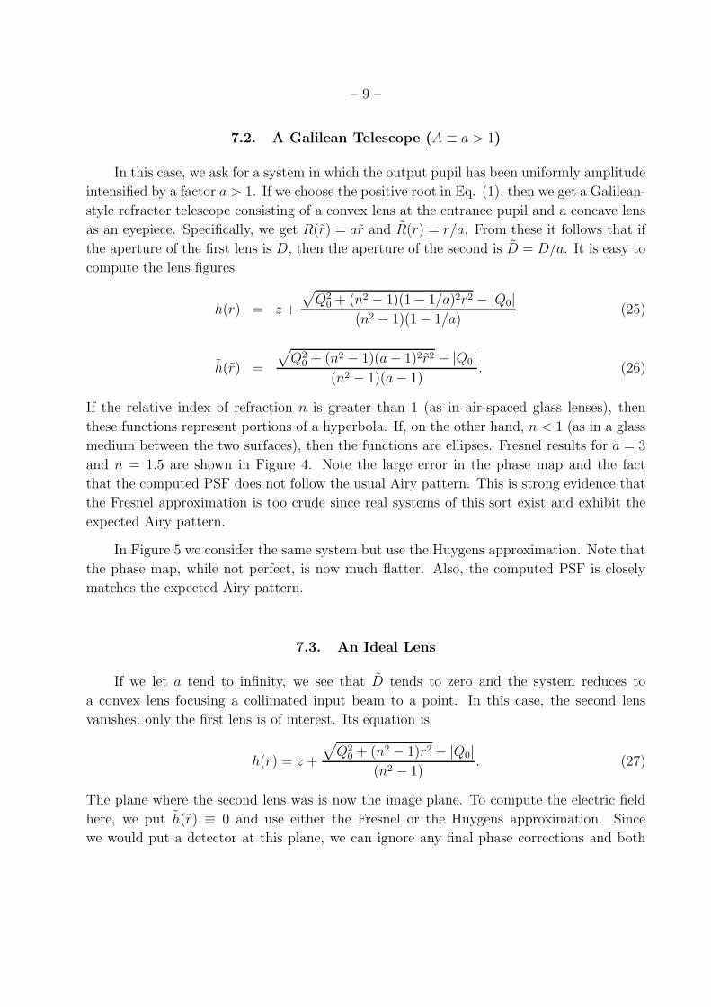
7.2. A Galilean Telescope (A ≡ a > 1)

In this case, we ask for a system in which the output pupil has been uniformly amplitude

intensified by a factor a > 1. If we choose the positive root in Eq. (1), then we get a Galilean-

style refractor telescope consisting of a convex lens at the entrance pupil and a concave lens

as an eyepiece. Specifically, we get R(r) = ar and R(r) = r/a. From these it follows that if

the aperture of the first lens is D, then the aperture of the second is D = D/a. It is easy to

compute the lens figures

h(r) = z +

√

Q20 + (n2 − 1)(1 − 1/a)2r2 − |Q0|

(n2 − 1)(1 − 1/a)(25)

h(r) =

√

Q20 + (n2 − 1)(a − 1)2r2 − |Q0|

(n2 − 1)(a − 1). (26)

If the relative index of refraction n is greater than 1 (as in air-spaced glass lenses), then

these functions represent portions of a hyperbola. If, on the other hand, n < 1 (as in a glass

medium between the two surfaces), then the functions are ellipses. Fresnel results for a = 3

and n = 1.5 are shown in Figure 4. Note the large error in the phase map and the fact

that the computed PSF does not follow the usual Airy pattern. This is strong evidence that

the Fresnel approximation is too crude since real systems of this sort exist and exhibit the

expected Airy pattern.

In Figure 5 we consider the same system but use the Huygens approximation. Note that

the phase map, while not perfect, is now much flatter. Also, the computed PSF is closely

matches the expected Airy pattern.

7.3. An Ideal Lens

If we let a tend to infinity, we see that D tends to zero and the system reduces to

a convex lens focusing a collimated input beam to a point. In this case, the second lens

vanishes; only the first lens is of interest. Its equation is

h(r) = z +

√

Q20 + (n2 − 1)r2 − |Q0|

(n2 − 1). (27)

The plane where the second lens was is now the image plane. To compute the electric field

here, we put h(r) ≡ 0 and use either the Fresnel or the Huygens approximation. Since

we would put a detector at this plane, we can ignore any final phase corrections and both

– 10 –

approximations reduce to the same formula:

Eout(r) =2π

λZ

∫

eπi r2

zλ−2πi

(n−1)h(r)λ J0(2πrr/zλ)rdr. (28)

Substituting Eq. (27) into Eq. (28) and dropping any unit complex numbers that factor out

of the integral, we get

Eout(r) =2π

λZ

∫

eπi r2

zλ−

2πiλ �(n−1

n+1)2z2+ n−1

n+1r2

J0(2πrr/zλ)rdr. (29)

Of course, this formula is for a uniform collimated input beam. If the input beam happens

to be pre-apodized by some upstream optical element, then the expression becomes

Eout(r) =2π

λZ

∫

eπi r2

zλ−

2πiλ �(n−1

n+1)2z2+ n−1

n+1r2

J0(2πrr/zλ)A(r)rdr (30)

where A(r) denotes the pre-apodization function. This formula does not agree with the

Fourier transform expression given earlier by equation Eq. (5). However, if the square root

is approximated by the first two terms of its Taylor expansion,

√

(

n − 1

n + 1

)2

z2 +n − 1

n + 1r2 =

n − 1

n + 1z +

r2

2z, (31)

then Eq. (30) reduces to a Fourier transform as in Eq. (5) (again dropping unit complex

factors).

This raises an interesting question: if a high-contrast amplitude profile is designed based

on the assumption that the focusing element behaves like a Fourier transform (i.e., as in Eq.

(5)), how well will the profile work if the true expression for the electric field is closer to

the one given by Eq. (30)? The answer is shown in Figure 6. The PSF degradation is very

small.

8. High-Contrast Pupil Mapping

The purpose of the examples discussed in the previous section was to convince the

reader that the Huygens approximation provides a reasonable estimate of the electric field

at the exit pupil of a pupil mapping system. Assuming we were convincing, we now proceed

to apply the Huygens approximation to compute the electric field and focused PSF of the

pupil mapping system corresponding to the amplitude profile function shown in Figure 2. As

before, we assume a wavelength of 0.6328µ and lenses with aperture D = 25mm. In Figure

– 11 –

7, we show the results for z = 15D and a refraction index of 1.5. For these simulations to

be meaningful, it is critical that the integrals be represented by a sum over a sufficiently

refined partition. The bigger the disparity between wavelength λ and aperture D, the more

refined the partition needs to be. For the parameters we have chosen, a partition into 5000

parts proved to be adequate. The plot in the upper-left section of the figure shows in gray

the target amplitude profile and in black the amplitude profile computed using the Huygens

approximation (i.e., equation Eq. (24)). The plot in the upper right shows the lens profiles.

The first lens is shown in black and the second in gray. The plot in the lower left shows

in gray the computed optical path length Q0(r). If the numerical computation of the lens

figures had been done with insufficient precision, this curve would not be flat. As we see,

it is flat. The lower left also shows in black the phase map as computed by the Huygens

approximation. Note that here there are high frequency oscillations everywhere and low

frequency oscillation that has an amplitude that increases as one moves out to the rim of

the lens. The lower-right plot shows in gray the PSF associated with the ideal amplitude

profile and in black the PSF computed by Huygens propagation.

The PSF in Figure 7 is disappointing. It is important to determine whether this is real

or is a result of the approximations behind the Huygens propagation formula. As a check,

we did a brute force computation of the Huygens integral Eq. (11). Because this integral is

more difficult, we were forced to use only 1000 r-values and 1000 θ-values. Hence, we had to

increase the wavelength by a factor of 5. With these changes, the result is shown in Figure

8. It too shows the same amplitude and phase oscillations. This sanity check convinces us

that these effects are physical. We need to consider changes to the physical setup that might

mollify these oscillations. Such changes are considered next.

There is no particular reason to make the two lenses have equal aperture. By scaling

the amplitude profile, we can easily generate examples with unequal aperture. One such

experiment we tried was to scale the amplitude function so that its value at the center is one

(thereby creating a traditional apodization). This scaling results in the second lens having

almost four times the aperture of the first lens. The results for this case are shown in Figure

9.

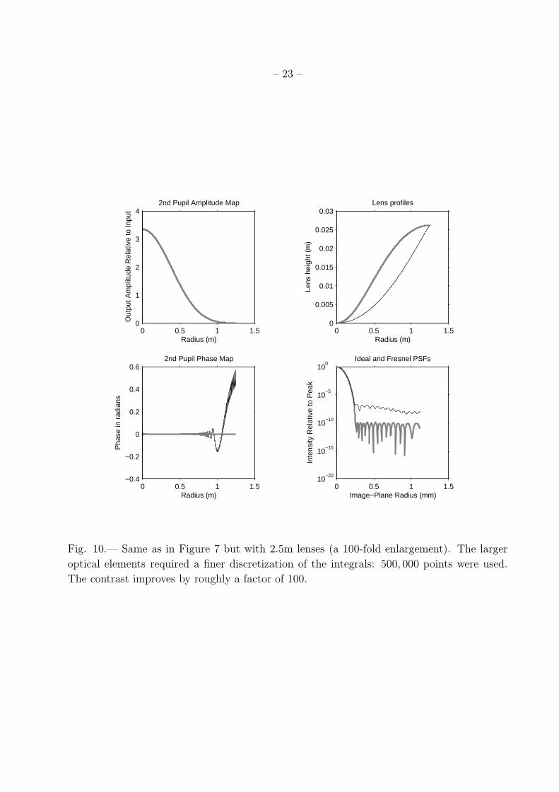
Another possibility is to consider larger optical elements—25mm is rather small. In

Figure 10 we show results for D = 2.5m (with z = 15D). The intensity of the first sidelobe

relative to the main lobe has improved by a factor of about 100 (3 × 10−5 vs. 3 × 10−7).

Clearly, the optics would need to be orders of magnitude larger in order to drive the contrast

to the 10−10 level.

If an amplitude profile designed for 10−10 contrast only produces 10−5, one wonders how

well a profile designed for 10−5 will do. The answer is shown in Figure 11. In this case, the

– 12 –

degradation due to diffraction effects is very small.

9. Hybrid Systems

If a pupil mapping system designed for 10−5 works well, perhaps it could be followed

by a conventional apodizer that attempts to bring the system from 10−5 down to 10−10. We

tried this. The result is shown in Figure 12. As can be seen in the lower-right plot, the

contrast achieved is limited to about 10−7.5. Apparently the diffraction ripples going into

the apodizer are enough to prevent the system from achieving the desired contrast.

As an alternative to a downstream apodizer, one could consider a pre-apodizer placed

in front of the first lens. Since it is generally hard edges that create bad diffraction effects,

we can imagine using the pre-apodizer to provide the near-outer-edge amplitude profile and

allow the pupil mapping system to provide the main body of the profile. In this way, perhaps

the diffraction effects can be minimized while at the same time maintaining a system with

high throughput. The results, shown in Figure 13, are comparable to those obtained with a

downstream apodizer.

Acknowledgements. This research was partially performed for the Jet Propulsion

Laboratory, California Institute of Technology, sponsored by the National Aeronautics and

Space Administration as part of the TPF architecture studies and also under JPL subcontract

number 1260535. The author also received support from the NSF (CCR-0098040) and the

ONR (N00014-05-1-0206).

REFERENCES

M. Born and E. Wolf. Principles of Optics. Cambridge University Press, New York, NY,

7th edition, 1999.

P.S. Carney and G. Gbur. Optimal apodizations for finite apertures. Journal of the Optical

Society of America A, 16(7):1638–1640, 1999.

A. Cumming, G.W. Marcy, R.P. Butler, and S.S. Vogt. The statistics of extrasolar planets:

Results from the keck survey. In D. Deming and S. Seager, editors, Scientific Frontiers

in Research on Extrasolar Planets, ASP Conference Series, 294, pages 27–30, 2002.

R. Galicher, O. Guyon, S. Ridgway, H. Suto, and M. Otsubo. Laboratory demonstration and

numerical simulations of the phase-induced amplitude apodization. In Proceedings of

the 2nd TPF Darwin Conference, 2004.

– 13 –

A. Goncharov, M. Owner-Petersen, and D. Puryayev. Intrinsic apodization effect in a com-

pact two-mirror system with a spherical primary mirror. Opt. Eng., 41(12):3111,

2002.

O. Guyon. Phase-induced amplitude apodization of telescope pupils for extrasolar terrerstrial

planet imaging. Astronomy and Astrophysics, 404:379–387, 2003.

O. Guyon, E.A. Pluzhnik, R. Galicher, R. Martinache, S.T. Ridgway, and R.A. Woodruff.

Exoplanets imaging with a phase-induced amplitude apodization coronagraph–i. prin-

ciple. Astrophysical Journal, 622:744, 2005.

J.A. Hoffnagle and C.M. Jefferson. Beam shaping with a plano-aspheric lens pair. Opt. Eng.,

42(11):3090–3099, 2003.

N.J. Kasdin, R.J. Vanderbei, D.N. Spergel, and M.G. Littman. Extrasolar Planet Finding

via Optimal Apodized and Shaped Pupil Coronagraphs. Astrophysical Journal, 582:

1147–1161, 2003.

J.L. Kreuzer. Coherent light optical system yielding an output beam of desired intensity

distribution at a desired equiphase surface, Nov 1969. U.S. Patent Number 3,476,463.

M.J. Kuchner, J. Crepp, and J. Ge. Finding terrestrial planets using eighth-order image

masks. Submitted to The Astrophysical Journal, 2004. (astro-ph/0411077).

M. Shao, B.M. Levine, E. Serabyn, J.K. Wallace, and D.T. Liu. Visible nulling coronagraph.

In Proceedings of SPIE Conference on Astronomical Telescopes and Instrumentation,

number 61 in 5487, 2004.

D. Slepian. Analytic solution of two apodization problems. Journal of the Optical Society

of America, 55(9):1110–1115, 1965.

W.A. Traub and R.J. Vanderbei. Two-Mirror Apodization for High-Contrast Imaging. As-

trophysical Journal, 599:695–701, 2003.

R. J. Vanderbei, N. J. Kasdin, and D. N. Spergel. Checkerboard-mask coronagraphs for

high-contrast imaging. Astrophysical Journal, 615(1):555, 2004.

R.J. Vanderbei, D.N. Spergel, and N.J. Kasdin. Circularly Symmetric Apodization via

Starshaped Masks. Astrophysical Journal, 599:686–694, 2003.

R.J. Vanderbei and W.A. Traub. Pupil Mapping in 2-D for High-Contrast Imaging. Astro-

physical Journal, 621?, 2005. To appear.

– 14 –

This preprint was prepared with the AAS LATEX macros v5.2.

– 15 –

−0.5 0 0.5−0.5

0

0.5

1

1.5

2

h r

r

h r

r R r

R r

z

Z

Fig. 1.— Pupil mapping via a pair of properly figured lenses.

−0.5 0 0.50

0.5

1

1.5

2

2.5

3

3.5

4

Pupil−Plane Radius in fraction of Aperture

Out

put A

mpl

itude

Rel

ativ

e to

Inpu

t

−60 −40 −20 0 20 40 6010

−16

10−14

10−12

10−10

10−8

10−6

10−4

10−2

100

Image−Plane Radius in L/D radians

Inte

nsity

Rel

ativ

e to

Pea

k

Fig. 2.— Left. An amplitude profile providing contrast of 10−10 at tight inner working

angles. Right. The corresponding on-axis point spread function.

– 16 –

0 0.005 0.01 0.0150.4

0.6

0.8

1

1.2

1.42nd Pupil Amplitude Map

Radius (m)

Out

put A

mpl

itude

Rel

ativ

e to

Inpu

t

6.1 6.2 6.3 6.4

x 10−3

0.97

0.98

0.99

1

1.01

1.02

1.03

1.04Amplitude Map Zoomed

Radius (m)

Out

put A

mpl

itude

Rel

ativ

e to

Inpu

t

0 0.005 0.01 0.015−1

−0.8

−0.6

−0.4

−0.2

0

0.2

0.42nd Pupil Phase Map

Radius (m)

Pha

se in

rad

ians

0 0.5 1 1.510

−8

10−6

10−4

10−2

100

Ideal and Fresnel PSFs

Image−Plane Radius (mm)

Inte

nsity

Rel

ativ

e to

Pea

k

Fig. 3.— Fresnel analysis of a pupil mapping system consisting of two flat pieces of n = 1.5

glass in circular D = 25-mm apertures separated by z = 15D. The wavelength is λ = 632.8-

nm. Upper-left plot shows in gray the target amplitude profile and in black the amplitude

profile computed using standard Fresnel propagation. Upper-right plot shows a zoomed in

section of the amplitude profiles. Lower-left plot shows in gray the computed optical path

length Q0(r) and in black the phase map computed using Fresnel propagation. Lower-right

plot shows in gray the PSF associated with the ideal amplitude profile and in black the PSF

computed by Fresnel propagation. These results should match textbook examples for simple

open circular apertures—and they do.

– 17 –

0 2 4 6 8

x 10−3

1

2

3

4

5

62nd Pupil Amplitude Map

Radius (m)

Out

put A

mpl

itude

Rel

ativ

e to

Inpu

t

0 0.01 0.02 0.030

0.5

1

1.5x 10

−3 Lens profiles

Radius (m)Le

ns h

eigh

t (m

)

0 2 4 6 8

x 10−3

−10

−5

0

5

10

15

202nd Pupil Phase Map

Radius (m)

Pha

se in

rad

ians

0 0.5 1 1.510

−10

10−5

100

105



Inte

nsity

Rel

ativ

e to

Pea

k

Fig. 4.— Same as in Figure 3 but with the apodization profile replaced with a constant

value of A ≡ 3. In this example, both lenses are hyperbolic as shown in the upper-right plot.

The lens profiles h and h were computed using a 5, 000 point discretization and the Fresnel

propagation (equation Eq. (19)) was carried out also with a 5, 000 point discretization. Note

the large error in the phase map and the fact that the computed PSF does not follow the

usual Airy pattern. This is strong evidence that the standard Fresnel approximation is too

crude since real systems of this sort exist and exhibit the expected Airy pattern.

– 18 –

0 2 4 6 8

x 10−3

0

1

2

3

4


Radius (m)

Out

put A

mpl

itude

Rel

ativ

e to

Inpu

t

0 0.01 0.02 0.030

0.5

1

1.5x 10

−3 Lens profiles

Radius (m)

Lens

hei

ght (

m)

0 2 4 6 8

x 10−3

−1

−0.8

−0.6

−0.4

−0.2

0

0.2


Radius (m)

Pha

se in

rad

ians

0 0.5 1 1.510

−8

10−6

10−4

10−2

100



Inte

nsity

Rel

ativ

e to

Pea

k

Fig. 5.— Same as in Figure 4 but computed using the Huygens approximation. Note that

the phase map is now much flatter. Also, the computed PSF closely matches the expected

Airy pattern.

– 19 –

0 0.2 0.4 0.6 0.8 1 1.2 1.410

−18

10−16

10−14

10−12

10−10

10−8

10−6

10−4

10−2

100



Inte

nsity

Rel

ativ

e to

Pea

k

Fig. 6.— The gray plot shows an ideal high-contrast PSF designed assuming that the

focussing element is a parabolic mirror so that the Huygens image-plane electric field is a

Fourier transform as in equation Eq. (5). The black line shows the PSF if one assumes that

the focussing element is actually an ideal lens (having an elliptical profile) as described in

Section 7.3. The two curves are visually identical except in the neighborhood of the 1st and

2nd minima of the Fourier (gray) curve.

– 20 –

0 0.005 0.01 0.0150

1

2

3

4


Radius (m)

Out

put A

mpl

itude

Rel

ativ

e to

Inpu

t

0 0.005 0.01 0.0150

1

2

3x 10

−4 Lens profiles

Radius (m)

Lens

hei

ght (

m)

0 0.005 0.01 0.015−0.2

0

0.2

0.4

0.6


Radius (m)

Pha

se in

rad

ians

0 0.5 1 1.510

−20

10−15

10−10

10−5

100



Inte

nsity

Rel

ativ

e to

Pea

k

Fig. 7.— Analysis of a pupil mapping system using the Huygens approximation with z = 15D

and n = 1.5. Upper-left plot shows in gray the target amplitude profile and in black the

amplitude profile computed using the Huygens approximation. Upper-right plot shows the

lens profiles, black for the first lens and gray for the second. The lens profiles h and h were

computed using a 5, 000 point discretization. Lower-left plot shows in gray the computed

optical path length Q0(r) and in black the phase map computed using Huygens propagation.

The Huygens propagation was carried out with a 5, 000 point discretization. Lower-right

plot shows in gray the PSF computed as the square of the Fourier transform of the ideal

amplitude profile and in black the PSF computed using the Huygens approximation.

– 21 –

0 0.005 0.01 0.0150

1

2

3

4


Radius (m)

Out

put A

mpl

itude

Rel

ativ

e to

Inpu

t

0 0.005 0.01 0.0150

1

2

3x 10

−4 Lens profiles

Radius (m)Le

ns h

eigh

t (m

)

0 0.005 0.01 0.015−0.4

−0.2

0

0.2

0.4

0.6

0.8

12nd Pupil Phase Map

Radius (m)

Pha

se in

rad

ians

0 0.5 1 1.510

−20

10−15

10−10

10−5

100



Inte

nsity

Rel

ativ

e to

Pea

k

Fig. 8.— Same as in Figure 7 but computed using a brute force computation of the Huygens

integral Eq. (11). Here we used 1000 r-values and 1000 θ-values. Consequently, we needed

to increase the wavelength by a factor 5 to guarantee adequate sampling of the phase and

amplitude ripples.

– 22 –

0 0.02 0.04 0.060

0.2

0.4

0.6

0.8

1

1.2


Radius (m)

Out

put A

mpl

itude

Rel

ativ

e to

Inpu

t

0 0.02 0.04 0.06−2.5

−2

−1.5

−1

−0.5

0

0.5x 10

−3 Lens profiles

Radius (m)

Lens

hei

ght (

m)

0 0.02 0.04 0.06−0.2

0

0.2

0.4

0.6


Radius (m)

Pha

se in

rad

ians

0 0.5 1 1.510

−20

10−15

10−10

10−5

100



Inte

nsity

Rel

ativ

e to

Pea

k

Fig. 9.— Same as in Figure 7 but with the amplitude profile normalized to a maximum value

of one. This normalization results in the two lenses having different apertures, the second is

about 4 times that of the first.

– 23 –

0 0.5 1 1.50

1

2

3


Radius (m)

Out

put A

mpl

itude

Rel

ativ

e to

Inpu

t

0 0.5 1 1.50

0.005

0.01

0.015

0.02

0.025

0.03Lens profiles

Radius (m)

Lens

hei

ght (

m)

0 0.5 1 1.5−0.4

−0.2

0

0.2

0.4


Radius (m)

Pha

se in

rad

ians

0 0.5 1 1.510

−20

10−15

10−10

10−5

100



Inte

nsity

Rel

ativ

e to

Pea

k

Fig. 10.— Same as in Figure 7 but with 2.5m lenses (a 100-fold enlargement). The larger

optical elements required a finer discretization of the integrals: 500, 000 points were used.

The contrast improves by roughly a factor of 100.

– 24 –

0 0.005 0.01 0.0150

0.5

1

1.5

2

2.5


Radius (m)

Out

put A

mpl

itude

Rel

ativ

e to

Inpu

t

0 0.005 0.01 0.0150

1

2

3x 10

−4 Lens profiles

Radius (m)Le

ns h

eigh

t (m

)

0 0.005 0.01 0.015−0.2

−0.1

0

0.1

0.2


Radius (m)

Pha

se in

rad

ians

0 0.5 1 1.510

−15

10−10

10−5

100



Inte

nsity

Rel

ativ

e to

Pea

k

Fig. 11.— The various sanity checks suggest that diffraction effects fundamentally limit

the close-in contrast attainable by pupil mapping to about 10−5. So, an amplitude profile

designed for 10−10 might not be the right one to use. Here, we show results for an amplitude

profile that only attempts to achieve 10−5. Note that the PSF via Huygens propagation

(black) agrees fairly well with the ideal (Fourier transform) PSF (gray) in the lower-right

plot.

– 25 –

0 0.005 0.01 0.0150

0.5

1

1.5

2

2.5


Radius (m)

Out

put A

mpl

itude

Rel

ativ

e to

Inpu

t

0 0.005 0.01 0.0150

1

2

3x 10

−4 Lens profiles

Radius (m)Le

ns h

eigh

t (m

)

0 0.005 0.01 0.015−0.2

−0.1

0

0.1

0.2


Radius (m)

Pha

se in

rad

ians

0 0.5 1 1.510

−15

10−10

10−5

100



Inte

nsity

Rel

ativ

e to

Pea

k

Fig. 12.— Given our success in Figure 11 of achieving 10−5 contrast with an amplitude profile

specifically designed for this level of contrast, we can now ask whether it is possible to put

a conventional apodizer (or shaped pupil equivalent) in the exit pupil to further “convert”

this amplitude profile into one that achieves 10−10. The result is shown here. As seen in the

PSF plots in the lower right, this combination gets the contrast to 10−7.5.

– 26 –

0 0.005 0.01 0.015 0.020

0.5

1

1.5

2

2.5

3


Radius (m)

Out

put A

mpl

itude

Rel

ativ

e to

Inpu

t

0 0.005 0.01 0.015 0.020

1

2

3

4x 10

−4 Lens profiles

Radius (m)Le

ns h

eigh

t (m

)

0 0.005 0.01 0.015−0.8

−0.6

−0.4

−0.2

0

0.2

0.4


Radius (m)

Pha

se in

rad

ians

0 0.5 1 1.510

−20

10−15

10−10

10−5

100



Inte

nsity

Rel

ativ

e to

Pea

k

Fig. 13.— As an alternative to the back-end apodizer considered in Figure 12, we consider

here the possibility of “softening” the edge of the first lens by using a pre-apodizer. The

dashed curve in the upper-left plot shows the pre-apodization function we used. As one can

see from the lower-right hand plot, this pre-apodization technique allows one to get the first

side-lobe almost down to the 10−7 level. This result is not quite as good as what we had

with the post-apodizer of Figure 12 but it is likely to be more manufacturable.

diffraction analysis of 2-d pupil mapping for high-contrast imaging

Documents