differential geometry in array processing (230 pages) · athanassios manikas imperial college...
TRANSCRIPT


DIFFERENTIAL GEOMETRY IN ARRAY
PROCESSING

This page intentionally left blank

Athanassios ManikasImperial College London, UK
DIFFERENTIAL GEOMETRY IN
A R R A YP R O C E S S I N G
Imperial College Press

British Library Cataloguing-in-Publication DataA catalogue record for this book is available from the British Library.
Published by
Imperial College Press57 Shelton StreetCovent GardenLondon WC2H 9HE
Distributed by
World Scientific Publishing Co. Pte. Ltd.
5 Toh Tuck Link, Singapore 596224
USA office: 27 Warren Street, Suite 401–402, Hackensack, NJ 07601
UK office: 57 Shelton Street, Covent Garden, London WC2H 9HE
Printed in Singapore.
For photocopying of material in this volume, please pay a copying fee through the CopyrightClearance Center, Inc., 222 Rosewood Drive, Danvers, MA 01923, USA. In this case permission tophotocopy is not required from the publisher.
ISBN 1-86094-422-1ISBN 1-86094-423-X (pbk)
Typeset by Stallion PressE-mail: [email protected]
All rights reserved. This book, or parts thereof, may not be reproduced in any form or by any means,electronic or mechanical, including photocopying, recording or any information storage and retrievalsystem now known or to be invented, without written permission from the Publisher.
Copyright © 2004 by Imperial College Press
DIFFERENTIAL GEOMETRY IN ARRAY PROCESSING
34_Differential Geometry.pmd 10/4/2005, 6:12 PM1

July 6, 2004 9:31 WSPC/Book Trim Size for 9in x 6in fm
To my wife, Eleni
v

This page intentionally left blank

July 6, 2004 9:31 WSPC/Book Trim Size for 9in x 6in fm
Preface
During the past few decades, there has been significant research intosensor array signal processing, culminating in the development of super-resolution array processing, which asymptotically exhibits infinite resolu-tion capabilities.
Array processing has an enormous set of applications and has recentlyexperienced an explosive interest due to the realization that arrays have amajor role to play in the development of future communication systems,wireless computing, biomedicine (bio-array processing) and environmentalmonitoring.
However, the “heart” of any application is the structure of the employedarray of sensors and this is completely characterized [1] by the array mani-fold. The array manifold is a fundamental concept and is defined as the locusof all the response vectors of the array over the feasible set of source/signalparameters. In view of the nature of the array manifold and its signifi-cance in the area of array processing and array communications, the roleof differential geometry as the most particularly appropriate analysis tool,cannot be over-emphasized.
Differential geometry is a branch of mathematics concerned with theapplication of differential calculus for the investigation of the properties ofgeometric objects (curves, surfaces, etc.) referred to, collectively, as “mani-folds”. This is a vast subject area with numerous abstract definitions,theorems, notations and rigorous formal proofs [2,3] and is mainly confinedto the investigation of the geometrical properties of manifolds in three-dimensional Euclidean space R3 and in real spaces of higher dimension.
However, the array manifolds are embedded not in real, but inN -dimensional complex space (where N is the number of sensors). There-fore, by extending the theoretical framework of R3 to complex spaces, the
vii

July 6, 2004 9:31 WSPC/Book Trim Size for 9in x 6in fm
viii Differential Geometry in Array Processing
underlying and under-pinning objective of this book is to present a sum-mary of those results of differential geometry which are exploitable and ofpractical interest in the study of linear, planar and three-dimensional arraygeometries.
Thanassis Manikas — London [email protected]
http://skynet.ee.imperial.ac.uk/manikas.html
Acknowledgments
This book is based on a number of publications (presented under a unifiedframework) which I had over the past few years with some of my formerresearch students. These are Dr. J. Dacos, Dr. R. Karimi, Dr. C. Proukakis,Dr. N. Dowlut, Dr. A. Alexiou, Dr. V. Lefkadites and Dr. A. Sleiman. I wishto express my pleasure in having had the opportunity in working with them.
I am indebted to my research associates Naveendra and Jason Ng aswell as to my MSc student Vincent Chan for reading, at various stages, themanuscript and for making constructive suggestions on how to improve thepresentation material.
Finally, I should like to thank Dr. P. Wilkinson who had the patience toread the final version of the manuscript. His effort is greatly appreciated.
Keywords
linear arrays, non-linear arrays, planar arrays, array manifolds, differentialgeometry, array design, array ambiguities, array bounds, resolution anddetection.

July 6, 2004 9:31 WSPC/Book Trim Size for 9in x 6in fm
Contents
Preface vii
1. Introduction 1
1.1 Nomenclature . . . . . . . . . . . . . . . . . . . . . . . . . . 31.2 Main Abbreviations . . . . . . . . . . . . . . . . . . . . . . 41.3 Array of Sensors — Environment . . . . . . . . . . . . . . . 51.4 Pictorial Notation . . . . . . . . . . . . . . . . . . . . . . . 8
1.4.1 Spaces/Subspaces . . . . . . . . . . . . . . . . . . . 81.4.2 Projection Operator . . . . . . . . . . . . . . . . . . 9
1.5 Principal Symbols . . . . . . . . . . . . . . . . . . . . . . . 111.6 Modelling the Array Signal-Vector and Array Manifold . . 111.7 Significance of Array Manifolds . . . . . . . . . . . . . . . . 171.8 An Outline of the Book . . . . . . . . . . . . . . . . . . . . 19
2. Differential Geometry of Array Manifold Curves 22
2.1 Manifold Curve Representation — Basic Concepts . . . . . 222.2 Curvatures and Coordinate Vectors in CN . . . . . . . . . . 26
2.2.1 Number of Curvatures and Symmetricityin Linear Arrays . . . . . . . . . . . . . . . . . . . . 26
2.2.2 “Moving Frame” and Frame Matrix . . . . . . . . . 282.2.3 Frame Matrix and Curvatures . . . . . . . . . . . . . 292.2.4 Narrow and Wide Sense Orthogonality . . . . . . . . 31
2.3 “Hyperhelical” Manifold Curves . . . . . . . . . . . . . . . 332.3.1 Coordinate Vectors and Array Symmetricity . . . . . 372.3.2 Evaluating the Curvatures of Uniform Linear Array
Manifolds . . . . . . . . . . . . . . . . . . . . . . . . 38
ix

July 6, 2004 9:31 WSPC/Book Trim Size for 9in x 6in fm
x Differential Geometry in Array Processing
2.4 The Manifold Length and Number of Windings(or Half Windings) . . . . . . . . . . . . . . . . . . . . . . . 41
2.5 The Concept of “Inclination” of the Manifold . . . . . . . . 452.6 The Manifold-Radii Vector . . . . . . . . . . . . . . . . . . 462.7 Appendices . . . . . . . . . . . . . . . . . . . . . . . . . . . 53
2.7.1 Proof of Eq. (2.24) . . . . . . . . . . . . . . . . . . . 532.7.2 Proof of Theorem 2.1 . . . . . . . . . . . . . . . . . 54
3. Differential Geometry of Array Manifold Surfaces 59
3.1 Manifold Metric . . . . . . . . . . . . . . . . . . . . . . . . 613.2 The First Fundamental Form . . . . . . . . . . . . . . . . . 623.3 Christoffel Symbol Matrices . . . . . . . . . . . . . . . . . . 643.4 Intrinsic Geometry of a Surface . . . . . . . . . . . . . . . . 65
3.4.1 Gaussian Curvature . . . . . . . . . . . . . . . . . . 663.4.2 Curves on a Manifold Surface: Geodesic Curvature . 68
3.4.2.1 Arc Length . . . . . . . . . . . . . . . . . . 693.4.2.2 The Concept of Geodicity . . . . . . . . . . 69
3.4.3 Geodesic Curvature . . . . . . . . . . . . . . . . . . 693.5 The Concept of “Development” . . . . . . . . . . . . . . . . 723.6 Summary . . . . . . . . . . . . . . . . . . . . . . . . . . . . 743.7 Appendices . . . . . . . . . . . . . . . . . . . . . . . . . . . 74
3.7.1 Proof of Eq. (3.36) — Geodesic Curvature . . . . . . 74
4. Non-Linear Arrays: (θ, φ)-Parametrization of ArrayManifold Surfaces 77
4.1 Manifold Metric and Christoffel Symbols . . . . . . . . . . 784.2 3D-grid Arrays of Omnidirectional Sensors . . . . . . . . . 804.3 Planar Arrays of Omnidirectional Sensors . . . . . . . . . . 814.4 Families of θ- and φ-curves on the Manifold Surface . . . . 834.5 “Development” of Non-linear Array Geometries . . . . . . . 874.6 Summary . . . . . . . . . . . . . . . . . . . . . . . . . . . . 934.7 Appendices . . . . . . . . . . . . . . . . . . . . . . . . . . . 93
4.7.1 Proof that the Gaussian Curvature of anOmni-directional Sensor Planar Array Manifold is Zero 93
4.7.2 Proof of the Expression of det G for Planar Arrays inTable 4.2 . . . . . . . . . . . . . . . . . . . . . . . . 94
4.7.3 Proof of “Development” Theorem 4.6 . . . . . . . . 95

July 6, 2004 9:31 WSPC/Book Trim Size for 9in x 6in fm
Contents xi
5. Non-Linear Arrays: (α, β)-Parametrization 97
5.1 Mapping from the (θ, φ) Parameter Spaceto Cone-Angle Parameter Space . . . . . . . . . . . . . . . 97
5.2 Manifold Vector in Terms of a Cone-Angle . . . . . . . . . 1005.3 Intrinsic Geometry of the Array Manifold Based on
Cone-Angle Parametrization . . . . . . . . . . . . . . . . . 1015.4 Defining the Families of α- and β-parameter Curves . . . . 1045.5 Properties of α- and β-parameter Curves . . . . . . . . . . 105
5.5.1 Geodecity . . . . . . . . . . . . . . . . . . . . . . . . 1055.5.2 Length of Parameter Curves . . . . . . . . . . . . . . 1075.5.3 Shape of α- and β-curves . . . . . . . . . . . . . . . 107
5.6 “Development” of α- and β-parameter Curves . . . . . . . 110
6. Array Ambiguities 113
6.1 Classification of Ambiguities . . . . . . . . . . . . . . . . . 1146.2 The Concept of an Ambiguous Generator Set . . . . . . . . 1186.3 Partitioning the Array Manifold Curve into Segments of
Equal Length . . . . . . . . . . . . . . . . . . . . . . . . . . 1216.3.1 Calculation of Ambiguous Generator Sets of Linear
(or ELA) Array Geometries . . . . . . . . . . . . . . 1306.4 Representative Examples . . . . . . . . . . . . . . . . . . . 1326.5 Handling Ambiguities in Planar Arrays . . . . . . . . . . . 135
6.5.1 Ambiguities on φ-curves . . . . . . . . . . . . . . . . 1366.5.2 Ambiguities on α-curves/β-curves . . . . . . . . . . 1396.5.3 Some Comments on Planar Arrays . . . . . . . . . . 1466.5.4 Ambiguous Generator Lines . . . . . . . . . . . . . . 149
6.6 Ambiguities and Manifold Length . . . . . . . . . . . . . . 1526.7 Appendices . . . . . . . . . . . . . . . . . . . . . . . . . . . 155
6.7.1 Proof of Theorem 6.1 . . . . . . . . . . . . . . . . . 155
7. More on Ambiguities: Symmetrical Arrays 157
7.1 Symmetric Linear Arrays and det(AN (s)) . . . . . . . . . . 1577.2 Characteristic Points on the Array Manifold . . . . . . . . 1597.3 Array Symmetricity and Non-Uniform Partitions
of Hyperhelices . . . . . . . . . . . . . . . . . . . . . . . . . 1637.4 Ambiguities of Rank-(N − 1) and Array Pattern . . . . . . 1677.5 Planar Arrays and ‘Non-Uniform’ Ambiguities . . . . . . . 1707.6 Conclusions . . . . . . . . . . . . . . . . . . . . . . . . . . . 172

July 6, 2004 9:31 WSPC/Book Trim Size for 9in x 6in fm
xii Differential Geometry in Array Processing
8. Array Bounds 174
8.1 Circular Approximation of an Array Manifold . . . . . . . . 1748.2 Accuracy and the Cramer Rao Lower Bound . . . . . . . . 179
8.2.1 Single Emitter CRB in Terms ofManifold’s Differential Geometry . . . . . . . . . . . 180
8.2.2 Two Emitter CRB in Terms of Principal Curvature . 1848.2.2.1 Elevation Dependence of Two Emitters’ CRB 1868.2.2.2 Azimuth Dependence of Two Emitters’ CRB 188
8.3 “Detection” and “Resolution” Thresholds . . . . . . . . . . 1908.3.1 Estimating the Detection Threshold . . . . . . . . . 1918.3.2 Estimating the Resolution Threshold . . . . . . . . . 194
8.4 Modelling of the Uncertainty Sphere . . . . . . . . . . . . . 1988.5 Thresholds in Terms of (SNR × L) . . . . . . . . . . . . . . 1998.6 Comments . . . . . . . . . . . . . . . . . . . . . . . . . . . 203
8.6.1 Schmidt’s Definition of Resolution . . . . . . . . . . 2038.6.2 CRB at the Resolution Threshold . . . . . . . . . . 2048.6.3 Directional Arrays . . . . . . . . . . . . . . . . . . . 205
8.7 Array Capabilities Based on α- and β-curves . . . . . . . . 2068.8 Summary . . . . . . . . . . . . . . . . . . . . . . . . . . . . 2088.9 Appendices . . . . . . . . . . . . . . . . . . . . . . . . . . . 209
8.9.1 Radius of Circular Approximation . . . . . . . . . . 2098.9.2 “Circular” and “Y” Arrays — Sensor Locations . . . 2108.9.3 Proof: CRB of Two Sources in Terms of κ1 . . . . . 210
Bibliography 215
Index 217

July 9, 2004 13:51 WSPC/Book Trim Size for 9in x 6in chap01
Chapter 1
Introduction
An array system is a collection of sensors (transducers) which are spatiallydistributed at judicious locations in the 3-dimensional real space, with acommon reference point. How the sensors are spatially distributed (arraygeometry) is influential not only on the overall array capabilities but also onits “abnormalities.” The type of the sensors varies with the application andsensors can take a wide variety of forms. Some common examples of sensorsinclude electromagnetic devices (such as RF antennas, optical receivers,etc.) and acoustic transducers (such as hydrophones, geophones, ultrasoundprobes, etc.).
The signals at the array elements contain both temporal and spatialinformation about the array signal environment which is usually contam-inated by background and sensor noise. Thus, the main aim of array pro-cessing is to extract and then exploit this spatio-temporal information tothe fullest extent possible in order to provide estimates of the parameters ofinterest of the array signal environment. Depending on the application, typ-ical parameters of interest associated with emitting sources (i.e. signals thatuse the same frequency and/or time-slot and/or code) can be the numberof incident signals, Directions-of-Arrival (DOAs), Times-of-Arrival (TOAs),ranges, velocities etc. Indeed, with an array system operating in the pres-ence of a number of emitting sources, and by observing the received arraysignal-vectors x(t), the following four general problems are of great interest:
(1) Detection problem — concerned with the determination/estimation ofthe number of incident signals. This problem is essentially the spa-tial analogue of model order selection in time-series analysis. Thus,the most popular methods for the solution of this problem are basedon “Akaike Information Criterion” (AIC) [4] and the “MinimumDescription Length” (MDL) criterion [5, 6]. Both methods involve the
1

July 9, 2004 13:51 WSPC/Book Trim Size for 9in x 6in chap01
2 Differential Geometry in Array Processing
minimization of a function of the noise eigenvalues of the array outputcovariance matrix.
(2) Parameter estimation problem — where various signal and channelparameters are estimated. One important problem of this type is the“Direction Finding” (DF). In this case the parameters of interest arethe bearings of emitters/targets (e.g. [7]). This problem is essentiallythe spatial analogue of the frequency estimation problem in time-seriesanalysis.
(3) Interference cancellation (or reception problem) — the acquisition ofone (desired) signal from a particular direction and the cancellation ofunwanted co-channel interfering signals (or jammers), from all otherdirections. When the desired signal and the interference occupy thesame frequency band, temporal filtering is inappropriate. However, thespatial separation of the sources can be exploited using an array of sen-sors (e.g. an antenna array). This operation falls, in array processingterms, under the general heading of “beamforming” while, in commu-nication systems terms, a beamformer is a “linear receiver” (e.g. [8]).
(4) Imaging — here the parameters of interest are the shapes and sizesof various objects in the environment. These are typically determinedby the generation of two- or three-dimensional maps depicting somefeature of the received signals (e.g. intensity) as a function of theirspatial coordinates (e.g. [9]).
The four types of problem described above are inter-related and thesolution to one problem may result in a partial or complete solution toanother. For example, the successful operation of all parametric parameterestimation algorithms requires solving firstly the detection problem (i.e.a priori knowledge of the number of emitters present). Furthermore, oncethe number and directions-of-arrival (DOAs) of signals received at the arraysite are estimated by solving the detection and direction-finding problems,nulls may be readily placed along the directions of the unwanted signals,hence achieving interference cancellation.
The applications of arrays in various scientific disciplines (such as theones already mentioned) are extensive and suffice to reveal the multi-dimensional significance of the array concept. For instance, although arrayprocessing has been extensively used in high frequency communications inthe past, the explosive growth in demand for cellular services in recent yearshas placed it at the centre of interest. Spatial diversity is considered to beone of the most promising solutions for increasing capacity and spectral

July 9, 2004 13:51 WSPC/Book Trim Size for 9in x 6in chap01
Introduction 3
efficiency. Indeed, the integration of array processing and communicationstechniques, exploiting the structure of antenna-array systems, has evolvedinto a well-established technology. This technology is moving from the con-ventional direction nulling and phase-arrays to advanced superresolutionspatiotemporal-arrays, MIMO array systems and arrayed wireless sensornetworks, which exploit the spatial and temporal properties of the channelin their quest to handle multipaths, and to increase capacity and spectralefficiency. Using these properties, an extra layer of co-channel interfer-ence (CCI) and inter-symbol-interference (ISI) cancellation is achieved —asymptotically providing complete interference cancellation.
The performance of array systems, especially the ones with super-resolution capabilities is, in general, limited by three main factors:
• The presence of inherent background and sensor noise.• The limited amount of information the sensors can measure due to finite
observation interval (number of snapshots) and array geometry.• The lack of calibration, modelling errors and system uncertainties
that are embedded in the received array signal-vector x(t), which arenot accounted for. Examples include uncertainties in mutual couplingbetween sensors, perturbations in the geometrical and electrical charac-teristics of the array, the presence of moving emitters, nonplanar wave-fronts, source angular/temporal spread, etc.
However, the overall quality of the system’s performance is naturally afunction of the array structure in conjunction with the geometrical charac-teristics of the signal environment, as well as the algorithms employed. Analgorithm would behave differently when used with different array struc-tures and, vice-versa, a certain array would generate different results whenits output is applied to different algorithms.
1.1 Nomenclature
It is assumed that the reader is familiar with the fundamentals of vector andmatrix algebra. In this book, for typographical convenience, matrices will bedenoted by blackboard bold symbols (e.g. A, T, I) or, in the absence of a cor-responding blackboard bold symbol, by boldface (e.g. r, k, Γ). Any under-lined symbol will represent a column vector, e.g. A, a, a. Derivatives withrespect to a general parameter p will be denoted with a “dot” (e.g. a), whilethe “prime” symbol (e.g. a′) will be reserved for differentiation with respect

July 9, 2004 13:51 WSPC/Book Trim Size for 9in x 6in chap01
4 Differential Geometry in Array Processing
to certain “invariant” parameters. The overall notation to be employed inthis book is as follows:
A, a ScalarA, a Column vectorA,A Matrix(·)T Transpose(·)H Hermitian transpose(·)† Pseudoinverse‖·‖F Frobenius norm of a matrix‖·‖ Norm of a vector| · | Magnitude, Hadamard (Schur) product and division respectively⊗ Kronecker productexp(A or A) Elementwise exponential of vector A or matrix A
expm(A) Matrix exponentialTr(A) Trace of matrix A
det(A) Determinant of A
diag(A) Diagonal matrix formed from the elements of A
diag(A) Column vector consisting of the diagonal elements of A
rowi (A) ith row of A
eleij (A) (ith, jth) element of A
fix(A) Round down to integerE· Expectation operatorAb Element by element power0N Zero vector of N elements1N Column vector of N onesIN N × N Identity matrixON×d N × d Zero matrixR Set of real numbersN Set of natural numbersZ Set of integer numbersC Field of complex numbers
1.2 Main Abbreviations
AGS Ambiguous Generator SetELA Equivalent Linear ArrayCRB Cramer Rao BoundDF Direction FindingDOA Directions of Arrival

July 9, 2004 13:51 WSPC/Book Trim Size for 9in x 6in chap01
Introduction 5
FOV Field-of-ViewSNR Signal-to-Noise RatioRMS Root Mean SquareULA Uniform Linear ArrayUCA Uniform Circular Array
1.3 Array of Sensors — Environment
By distributing, in the 3-dimensional Cartesian space, a number N 2of sensors (transducing elements, antennas, receivers, etc.) with a commonreference point, an array is formed. In general, the positions of the sensorsare given by the matrix r ∈ R3×N
r =[r1, r2, . . . , rN
]=
[rx, ry, rz
]T(1.1)
with rk = [xk, yk, zk]T ∈ R3×1 denoting the Cartesian coordinates (loca-tion) of the kth sensor of the array ∀k = 1, 2, . . . , N.
It is common practice to express the direction of a wave impinging onthe array in terms of the azimuth angle θ, measured anticlockwise from thepositive x-axis, and the elevation angle φ, measured anticlockwise from thex-y plane, as illustrated in Fig. 1.1. Then, the (3× 1) real unit-norm vector
Fig. 1.1 Relative geometry between a far-field emitting source and an array of sensors.

July 9, 2004 13:51 WSPC/Book Trim Size for 9in x 6in chap01
6 Differential Geometry in Array Processing
pointing towards the direction (θ, φ) is
u u(θ, φ) =[cos θ cos φ, sin θ cos φ, sin φ
]T(1.2)
Note that ‖u‖ = 1. If the velocity, wavelength and frequency of propaga-tion of the incident wave is denoted by c, λ and Fc, respectively, then thewavenumber vector in the direction (θ, φ) is defined as
k = k(θ, φ) =
2πFc
c· u =
2π
λ· u in meters
π · u in λ/2(1.3)
In the most general case, the parameter space is
Ω = (θ, φ) : θ ∈ [0, 360) and φ ∈ (−90, 90) (1.4)
but in most applications, Ω is restricted to only a sector of interest or,in other words, field-of-view (FOV). For instance, in the case of groundsurveillance radars, only signals in the plane of the array are of interest —i.e. the system is azimuth-only.
The array configuration is, to a large extent, dictated by the applicationof interest. One obvious restriction is the shape and size of the availablesite, which might be, to cite just a few examples, an aircraft’s wing, a ship’shull, a building rooftop, or simply a terrain. In addition, if the signals to beintercepted are known to be coplanar and within a 180 field-of-view, as inground and marine navigation applications, then a linear or 1-dimensional(1D) array of sensors may be sufficient.
(1) Linear or 1-dimensional (1D) Array.The linear or 1D array consists of a one-dimensional distribution ofsensors along a line conventionally taken as the x-axis (Fig. 1.2(a)),with sensor positions in units of half-wavelengths given by the matrix
r = [rx, 0N , 0N ]T ∈ R3×N (1.5)
where
rx = [r1, r2, . . . , rN ]T
The most popular array of this type is the standard UniformLinear Array (ULA) whose sensors are uniformly spaced at one half-wavelength apart along the x-axis. For example, a 5-sensor standard

July 9, 2004 13:51 WSPC/Book Trim Size for 9in x 6in chap01
Introduction 7
Fig. 1.2 Examples of array geometries: (a) linear array, (b) uniform circular array,(c) “cross” array.
ULA is given by rx = [−2,−1, 0, 1, 2]T in half wavelengths. Note thatthe phase reference, or origin of the coordinate system, is taken at thearray centroid. By exploiting the regular structure of the ULA, manyDF algorithms can be simplified allowing for significant computationalsavings. The FOV of 1D arrays is restricted to
Ω = (θ, φ) : θ ∈ [0, 180), φ = 0 (1.6)
It can be easily deduced from the geometry of the problem that a lin-ear array is incapable of distinguishing directions which are symmetricwith respect to the array line or which have the same elevation. If a360 FOV is instead required, then a planar or 2D array should beemployed.

July 9, 2004 13:51 WSPC/Book Trim Size for 9in x 6in chap01
8 Differential Geometry in Array Processing
(2) Planar or 2-dimensional (2D) Array.If the application of interest demands a full azimuthal FOV, that is,θ ∈ [0, 360), and possibly some elevation discrimination capability,then a planar or 2D array is necessary. A planar array consists of a twodimensional distribution of sensors over a plane, which is convention-ally taken as the x-y plane, and whose sensor positions are given by thematrix
r = [rx, ry, 0N ]T ∈ R3×N (1.7)
where rx and ry, respectively, are the column vectors of length N denot-ing the x- and y-coordinates of the sensors in units of half-wavelengths.The FOV of a planar array is the full azimuth space and half the ele-vation space
Ω = (θ, φ) : θ ∈ [0, 360), φ ∈ [0, 90) (1.8)
Note that a planar array cannot distinguish between directions whichare symmetric with respect to the array plane. Practical planar arraystructures include the grid, X, Y and L-shaped arrays, but the mostpopular is the uniform circular array (UCA) which, due to its symme-try, exhibits uniform performance over the entire azimuthal space [16].Fig. 1.2(b,c) illustrates two practical planar array (UCA and cross-array) configurations used in radio direction-finding systems operatingin the UK in the HF (3 to 30 MHz) band. It is important to point outthat a planar array also permits the discrimination of signals in eleva-tion φ ∈ [0, 90) — i.e. the emitters need not be coplanar (as is thecase in airborne surveillance), although its resolving power in the eleva-tion space is not as good as that of a 3D array. A 3D array has a FOVspanning the entire parameter space. However, for most applications1D and 2D arrays prove to be sufficient.
1.4 Pictorial Notation
1.4.1 Spaces/Subspaces
Because the visualization of a space greater than a 3-dimensional realspace is impossible, the notation shown in Fig. 1.3 is employed to pro-vide some illustrative aid. However, this pictorial representation should beused with care.

July 9, 2004 13:51 WSPC/Book Trim Size for 9in x 6in chap01
Introduction 9
Fig. 1.3 Illustrative Notation: (a) denotes a N -dimensional complex (or real) obser-vation space. Note that any vector in this space has N elements; (b) denotes a one-dimensional subspace/space spanned by the vector a; (c) denotes an M -dimensionalsubspace/space (with M ≥ 2) spanned by the columns of the matrix A.
1.4.2 Projection Operator
Consider an (N×M) matrix A with M < N (i.e. the matrix has M columns)and let L[A] represent the linear subspace spanned by the columns of A.Assuming that the columns of A are linearly independent — that is, acolumn of A cannot be written as a linear combination of the remainingM − 1 columns — the subspace L[A] is of dimensionality M, i.e.
dim L[A] = M < N (1.9)
lying in a N -dimensional space H, as shown in Fig. 1.4. The complementsubspace to L[A] is denoted by L[A]⊥ and is of dimensionality N − M , i.e.
dim
L[A]⊥
= N − M (1.10)
Then:
(1) any vector x ∈ L[A] can be written as a linear combination of thecolumns of the matrix A
(2) any vector x ∈ H can be projected onto L[A] (or onto L[A]⊥), asshown in Fig. 1.5, using the concept of the projection operator definedas follows:
PA = projection operator onto the subspace L[A]
= A(AH A)−1AH (1.11)

July 9, 2004 13:51 WSPC/Book Trim Size for 9in x 6in chap01
10 Differential Geometry in Array Processing
P⊥A = the projection operator onto L[A]⊥
= IN − PA (1.12)
N.B.: Properties of PA
(N × N) matrix
PA PA = PA
PA = PHA
(1.13)
Fig. 1.4 Illustrative representation of the subspaces L[A] and L[A]⊥ lying in anN -dimensional complex space.
Fig. 1.5 Illustrative representation of the projection of any vector x ∈ H onto L[A] andonto L[A]⊥.

July 9, 2004 13:51 WSPC/Book Trim Size for 9in x 6in chap01
Introduction 11
(3) For any vector x ∈ L[A] the following expressions are validPA x = x
P⊥A
x = 0N
(1.14)
1.5 Principal Symbols
In this book the following symbols will always denote
p, q generic parametersθ azimuth angleφ elevation angleα alpha — cone angleβ beta — cone angles arc lengthN number of sensorsr (3 × N) real matrix with columns the sensor locationsa array manifold vectorlm array manifold lengthla array apertureA array manifold curveM array manifold surfaceH space/subspace
1.6 Modelling the Array Signal-Vector andArray Manifold
Consider an array of N sensors, with sensor locations r, operating in thepresence of M narrowband point sources and having the same known carrierfrequency Fc. The modelling of the signal due to the ith emitter, receivedat the zero-phase reference point (taken to be the origin of the coordinatesystem) is determined by whether the source is located in, or close to, thearray’s near-field or in the array’s far-field. In practice, this is determinedaccording to the value of its range ρi with respect to the array aperture la,defined as follows:
la = max∀i,j
∥∥ri − rj
∥∥ (1.15)

July 9, 2004 13:51 WSPC/Book Trim Size for 9in x 6in chap01
12 Differential Geometry in Array Processing
To be more specific, if ρi 2la/λ, where λ is the wavelength of the trans-mitted signals, the ith source is located close to the array near-field border(which defines the so-called Fresnel zone) and the spherical wave prop-agation model has to be considered. For ρi > 2la/λ and especially forρi 2la/λ, the ith source is situated in the array far-field (the so-calledFraunhofer zone) and plane wave propagation is assumed. As a matter offact, sources of range ρi 2la/λ or ρi > 2la/λ, but not ρi 2la/λ, areusually regarded as being located in the near far-field of an array, for whichthe spherical wave propagation model has to be utilized.
Based on the above discussion and by considering the M sources in thefar-field of the array, the array signal is the superposition of plane wavesfrom each individual source. The planewave/signal due to the ith emitter,received at the zero-phase reference point, can be written as
ith signal at the reference point: mi(t) exp(j2πFct) (1.16)
where mi(t) represents the complex envelope (message) of the signal andexp(j2πFct) represents the carrier. If τik represents the propagation delayof the ith signal between the phase reference location and the kth sensorthen the signal arriving at the kth sensor will be a delayed version of thesignal given in Eq. (1.16), expressed as shown below
ith signal at the kth sensor: mi(t − τik)︸ ︷︷ ︸≈mi(t)
exp(j2πFc(t − τik)) (1.17)
This propagation delay τik is a function of the DOA of the ith signal andthe position of the kth sensor with respect to the reference point. Indeed,with reference to Fig. 1.6, τik can be derived as
τik =ik
c=
∥∥Puirk
∥∥c
=
√rT
k PTui
Puirk
c
=
√rT
k Puirk
c(using Eq. (1.13))
=
√rT
k ui
(uT
i ui
)−1uT
i rk
c

July 9, 2004 13:51 WSPC/Book Trim Size for 9in x 6in chap01
Introduction 13
Fig. 1.6 Geometry of a travelling plane wave, relative to the kth sensor and the arrayreference point.
=
√rT
k ui uTi rk
c=
√(rT
k ui
)2c
=rT
k ui
c
i.e.
τik =rT
k ui
c(1.18)
It is reasonable to assume that the envelope (baseband signal mi(t)) doesnot change significantly as it traverses the array. Hence τik τmax,∀i, k
and mi(t − τmax) mi(t) has been used in Eq. (1.17), where τmax is themaximum possible time for a signal to traverse the array. This is due to thenarrowband assumption, i.e. the highest frequency in the message signal

July 9, 2004 13:51 WSPC/Book Trim Size for 9in x 6in chap01
14 Differential Geometry in Array Processing
is much less than the carrier frequency. By taking into account the aboveassumption, as well as the complex response (gain and phase) γk(θi, φi) ofthe kth sensor at frequency Fc in the azimuth-elevation direction (θi, φi),the received signal at the kth sensor due to the ith emitting source can bewritten as
γk(θi, φi) · mi(t) · exp(
−j2πFcrT
k · ui
c
)exp(j2πFct)
= γk(θi, φi) · mi(t) · exp(−jrTk · ki) exp(j2πFct) (1.19)
where ki = k(θi, φi) denotes the wavenumber vector in the direction of theith emitter.
Next, the received signal is downconverted to baseband by multiplyingwith exp(−j2πFct). The baseband signal at the output of the kth sensor,in the presence of M far-field emitters and additive baseband noise nk(t)can be written as
xk(t) =M∑i=1
γk(θi,φi) mi(t) exp(−j rTk ki) + nk(t) (1.20)
Using vector notation, the output from all the N sensors, can beexpressed as
x(t) =[x1(t), x1(t), . . . , xN (t)
]T=
M∑i=1
mi(t)ai + n(t) (1.21)
where n(t) =[n1(t) n2(t) · · · nN (t)
]T ∈ CN×1 denotes the basebandadditive white Gaussian noise of power σ2. The (N × 1) complex vectorai is known as the array manifold vector associated with the ith emittingsource (signal), representing the complex array response to a unit amplitudeplane wave impinging from direction (θi, φi), compactly written as
ai a(θi, φi) = γ(θi, φi) exp
−j [rx, ry, rz]︸ ︷︷ ︸=rT
k(θi, φi)
(1.22)
whereγ(θi, φi) = [γ1(θi,φi), γ2(θi, φi), . . . , γN (θi, φi)]T ∈ CN×1

July 9, 2004 13:51 WSPC/Book Trim Size for 9in x 6in chap01
Introduction 15
This vector is also referred to as the “array response vector” or “arraysteering vector.”
Given that the same array may be represented by an infinite numberof matrices r through a change in the coordinate system reference point, achoice is made to fix the coordinate reference point (0, 0, 0) to be the arraycentroid. This translates into a condition on the location vectors rx, ry andrz such that
sum(rx) = sum(ry) = sum(rz) = 0 (1.23)
or equivalently,rT
x 1N = rTy 1N = rT
z 1N = 0 (1.24)
As can be seen from Eq. (1.22), a shift in the reference point of the arraycoordinate system results in a manifold vector ar(θ, φ) which is related tothe initial manifold vector:
ar (θ, φ) = g (θ, φ) · a (θ, φ) (1.25)
where g(θ, φ) is a complex number with |g(θ, φ)| = 1,∀(θ, φ). In fact,g(θ, φ) = exp(−jrT
0 k(θ, φ)) where r0 is the translation vector of the ref-erence point from the centroid of the array. For simplicity, all arrayshenceforth will have their centroid as the coordinate reference point, i.e.g(θ, φ) = 1,∀(θ, φ).
Note that in the case of a linear array of isotropic sensors Eq. (1.22)simplifies to
a(θ) = exp(−jπrx cos θ) (1.26)
while for a planar array it takes the following form:
a(θ, φ) = exp(−jπr(θ) cos φ) (1.27)
where
r(θ) = rx cos θ + ry sin θ (1.28)
It can easily be seen that r(θ) in Eq. (1.27) represents the positions ofthe projections of the sensor locations of the planar array onto the line ofazimuth θ (see Fig. 1.7), and is known as the “Equivalent Linear Array”(ELA) along the direction θ. Notice the similarity between the response

July 9, 2004 13:51 WSPC/Book Trim Size for 9in x 6in chap01
16 Differential Geometry in Array Processing
Fig. 1.7 Equivalent Linear Array (ELA) associated with the azimuth angle θ.
vectors of the linear and planar arrays in Eqs. (1.26) and (1.27) respectively.Using Eq. (1.22) the observed array signal-vector x(t) ∈ CN×1 of Eq. (1.21)can be written concisely as
x(t) = Am(t) + n(t) (1.29)
where A =
[a1,a2, . . . ,aM
]m(t) = [m1, m2, . . . , mM ]T
(1.30)
where A ∈ CN×M is the array manifold (response) matrix and m(t) ∈ CM×1
is the vector of signal envelopes (messages). Note that in the case of isotropicsensors the matrix A can be written in a compact way as
A = exp(−jrT k) (1.31)
with k = [k1, k2, . . . , kM ] representing the wavenumber matrix.Based on the above model of Eq. (1.29), the theoretical covariance
matrix Rxx of the array signal-vector x(t) can be formed as
Rxx Ex(t) x(t)H ∈ CN×N
= ARmmAH + σ2IN (1.32)

July 9, 2004 13:51 WSPC/Book Trim Size for 9in x 6in chap01
Introduction 17
where Rmm Em(t) m(t)H ∈ CM×M is the source covariance matrix,which is diagonal in the case of uncorrelated signals and σ2IN is the addi-tive white Gaussian noise covariance matrix Rnn En(t) n(t)H ∈ CN×N .In practice, only a finite number L data snapshots [x(t1), x(t2), . . . , x(tL)],collected by an array of sensors, can be observed. Hence only an esti-mate of Rxx is computed in the form of the sample covariance matrixgiven by
Rxx 1L
L∑i=1
x(ti) x(ti)H =1L
XXH (1.33)
where
X [x(t1), x(t2), . . . , x(tL)] ∈ CN×L
It is important to point out that if the assumption mi(t − τik) ≈mi(t),∀i, k used in Eq. (1.17) is not valid, then the array signal vectorassociated with the ith signal should be modelled as
x(t) =M∑i=1
mτi(t) ai + n(t) (1.34)
where
mτi(t) = [mi(t − τi1), mi(t − τi2), . . . , mi(t − τiN )]T
1.7 Significance of Array Manifolds
It is clear from Eqs. (1.22), (1.26) or (1.27) that the manifold vector fora particular direction contains all the information about the geometryinvolved when a wave is incident on the array from that direction. Byrecording the locus of the manifold vectors as a function of direction, a“continuum” (i.e. a geometrical object such as a curve or surface) is formedlying in an N -dimensional space. This geometrical object (locus of manifold,or response, vectors) is known as the array manifold. The array manifoldcan be calculated (and stored) from only the knowledge of the locations anddirectional characteristics of the sensors. Thus, according to Schmidt [1],“the array manifold completely characterizes any array and provides a rep-resentation of the real array into N -dimensional complex space.”
The significance of the array manifold concept becomes apparent when itis realized that all subspace-based parameter estimation algorithms involvesearching over the array manifold for response vectors which satisfy a
July 9, 2004 13:51 WSPC/Book Trim Size for 9in x 6in chap01
18 Differential Geometry in Array Processing
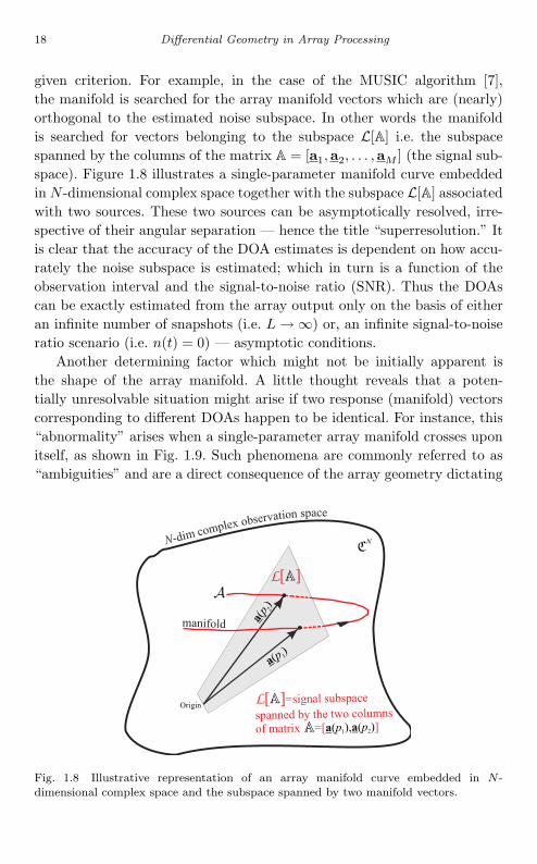
given criterion. For example, in the case of the MUSIC algorithm [7],the manifold is searched for the array manifold vectors which are (nearly)orthogonal to the estimated noise subspace. In other words the manifoldis searched for vectors belonging to the subspace L[A] i.e. the subspacespanned by the columns of the matrix A = [a1,a2, . . . ,aM ] (the signal sub-space). Figure 1.8 illustrates a single-parameter manifold curve embeddedin N -dimensional complex space together with the subspace L[A] associatedwith two sources. These two sources can be asymptotically resolved, irre-spective of their angular separation — hence the title “superresolution.” Itis clear that the accuracy of the DOA estimates is dependent on how accu-rately the noise subspace is estimated; which in turn is a function of theobservation interval and the signal-to-noise ratio (SNR). Thus the DOAscan be exactly estimated from the array output only on the basis of eitheran infinite number of snapshots (i.e. L → ∞) or, an infinite signal-to-noiseratio scenario (i.e. n(t) = 0) — asymptotic conditions.
Another determining factor which might not be initially apparent isthe shape of the array manifold. A little thought reveals that a poten-tially unresolvable situation might arise if two response (manifold) vectorscorresponding to different DOAs happen to be identical. For instance, this“abnormality” arises when a single-parameter array manifold crosses uponitself, as shown in Fig. 1.9. Such phenomena are commonly referred to as“ambiguities” and are a direct consequence of the array geometry dictating
Fig. 1.8 Illustrative representation of an array manifold curve embedded in N -dimensional complex space and the subspace spanned by two manifold vectors.

July 9, 2004 13:51 WSPC/Book Trim Size for 9in x 6in chap01
Introduction 19
Fig. 1.9 Illustrative representation of array “abnormality” (ambiguity).
the behavior of the array manifold. As will be discussed below, the behaviorof the array manifold, in particular its local geometry, plays an importantrole in handling “abnormalities” and also in defining the capabilities (e.g.the resolving power) of an array system.
1.8 An Outline of the Book
The theoretical framework associated with curves lying in N -dimensionalcomplex space, qualifying to be manifolds of linear array structures, ispresented in Chapter 2. More specifically by recording the locus of thevector a(p) as a function of p, a one-dimensional continuum (i.e. a curve A)is formed known as the array manifold and embedded in a N -dimensionalspace. Thus in this chapter the properties and characteristics of single-parameter manifolds (i.e. curves) are investigated and supported by a num-ber of representative examples of symmetric and non-symmetric linear arraygeometries [10]. These manifold curves have been found to have a hyper-helical shape with numerous advantages. For example, all the curvaturesof a hyperhelix are constant (do not vary from point to point) and maybe evaluated recursively. The convenient nature of a hyperhelix’s geometrywill be proven invaluable for the rest of the book, not only for linear butalso for non-linear (2D and 3D) arrays.

July 9, 2004 13:51 WSPC/Book Trim Size for 9in x 6in chap01
20 Differential Geometry in Array Processing
If the manifold vector a corresponds to two parameters (p,q) where,for instance p may be the azimuth and q the elevation angle, then a2-dimensional continuum, i.e. a surface M, is formed by recording the locusof the vector a(p, q) as a function of both p and q. Chapter 3 is concernedwith the study of manifold surfaces embedded in a multidimensional com-plex space and presents the essential differential geometry parameters whichhave been grouped into those related to the surface itself, and those relatedto curves lying on a surface [11]. Then a manifold surface is treated asa family of curves on the surface by an appropriate parametrization. Thistreatment is very convenient as it permits a unified framework for the analy-sis of the linear and non-linear array manifolds. To provide a simplifiedrepresentation of the analysis, with many potential benefits, the conceptof isometric mapping is also introduced in Chapter 3. Then an isometricmapping of the manifold surface (embedded in a multidimensional com-plex space) onto the real plane (two-dimensional space) is presented whichpreserves certain differential geometry characteristics of the manifold sur-face, under certain conditions.
It is common practice, and intuitively appealing, in array processingto use azimuth and elevation as the directional parameters of a waveformimpinging on an array of sensors. However, this is by no means uniqueand, furthermore, this is not the most suitable parametrization for thestudy of the behavior of the array manifold [12]. Therefore in Chapters 4and 5, based on the material presented in Chapters 2 and 3, the followingmanifold-surface parametrizations
• the (azimuth, elevation), or (θ, φ), parametrization• the cone-angles, or (α, β), parametrization
are examined for non-linear arrays (2D and 3D geometries). The significanceof these parametrizations is demonstrated by a number of representativeexamples. Furthermore, properties such as Gaussian and geodesic curva-tures are defined and their implications with regards to isometric mappingsare discussed.
In the next two chapters of the book (Chapters 6 and 7) the funda-mental effects of the array geometry behavior on the performance of thesystem irrespective of the type of algorithm used, are studied. The arraystructure is incorporated into the observed array signal-vectors x(t) (andtherefore to the estimation problem) through the array manifold. Thus thegeometry of an array plays a crucial role in dictating the shape, properties

July 9, 2004 13:51 WSPC/Book Trim Size for 9in x 6in chap01
Introduction 21
and “anomalies” of the array manifold, and as a consequence, in dictat-ing the phenomenon where some manifold vectors can be written as linearcombinations of others [13,25]. This gives rise to the array “ambiguity prob-lem” where the occurrence of false parameter estimates seriously impairsthe performance of array system irrespective of its other capabilities. Inparticular, in Chapters 6 and 7 two general types of ambiguities are pre-sented based on the partitioning of the array manifold curves into equal orunequal segments from which the ambiguous generator sets (AGS) can beconstructed — with each AGS representing an infinite number of ambigu-ous sets of parameter values (e.g. directions). Furthermore, the theoreticalaspects of the investigation provide a sufficient condition for the presenceof ambiguities while the results are then extended to non-linear arrays bytreating surfaces as families of curves [14].
Finally, in Chapter 8, the knowledge of the shape of the array mani-fold is used to determine the array’s ultimate capabilities according to thefollowing criteria:
• Accuracy and the Cramer Rao Lower Bound• Detection threshold• Resolution threshold
In particular, by approximating, locally, a manifold curve with a circulararc, the Cramer Rao Lower Bound (CRB) is studied and its relation toresolution and detection bounds is established [15, 16]. Then by definingthe detection and resolution subspaces, in conjunction with the circularapproximation (locally) of the array manifold, the minimum arc lengthseparation in order to detect and resolve two sources located close togetheris estimated. This is done in terms of the curve’s principal curvature only,thereby simplifying the analysis considerably.

July 6, 2004 9:29 WSPC/Book Trim Size for 9in x 6in chap02
Chapter 2
Differential Geometry of ArrayManifold Curves
2.1 Manifold Curve Representation — Basic Concepts
Let a a(p) ∈ CN be the manifold vector of an array of N sensors where p
is a generic directional parameter. This is a single-parameter vector functionand as p varies the point a will trace out a curve A, as shown in Fig. 2.1,embedded in an N -dimensional complex space CN . This was expected, asvector functions of one parameter are used to define space curves — alsoknown as single-parameter manifolds.
The curve A, which is formally defined
A a(p) ∈ CN , ∀p : p ∈ Ωp
(2.1)
where Ωp denotes the parameter space, is said to be a regular parametrizeddifferential curve if
a(p) = 0N , ∀p ∈ Ωp (2.2)
where a “dot” at the top of a symbol is used to denote differentiationwith respect to parameter p. As the vector a(p) represents the tangentvector to the curve, the “regularity” condition of Eq. (2.2) ensures that thetangent vector exists at all points on the array manifold. The arc lengths(p) along the manifold curve A and its rate-of-change s(p) are formallydefined, respectively, as
s(p) ∫ p
0
‖a(p)‖ dp (2.3)
ands(p) =
ds
dp ‖a(p)‖ (2.4)
22

July 6, 2004 9:29 WSPC/Book Trim Size for 9in x 6in chap02
Differential Geometry of Array Manifold Curves 23
Fig. 2.1 Manifold curve A embedded in CN .
Fig. 2.2 Manifold parameterization in terms of arc length s.
The array manifold is conventionally parametrized in terms of a genericbearing parameter p. For instance for a linear array, p may represent theazimuth angle θ. However, parametrization in terms of the arc length s (seeFig. 2.2), which is the most basic feature of a curve and a natural parameterrepresenting the actual physical length of a segment of the manifold curve in

July 6, 2004 9:29 WSPC/Book Trim Size for 9in x 6in chap02
24 Differential Geometry in Array Processing
CN , is more suitable. There is a further advantage of using s as a parameter:the arc length s (in contrast to p) is an “invariant” parameter. This meansthat the resulting tangent vector to the curve, expressed in terms of s,always has unity length. Indeed, it can be seen that
‖a′(s)‖ =∥∥∥∥da(s)
ds
∥∥∥∥ =∥∥∥∥da(p)/dp
ds/dp
∥∥∥∥ =‖a(p)‖s(p)
=s(p)s(p)
= 1, ∀s (2.5)
which is a result used next in defining the unit tangent vector u1(s) (seeFig. 2.3)
u1(s) a′(s) (2.6)
Unless otherwise stated, differentiation with respect to s will be denotedby “prime” and differentiation with respect to any other parameter p willbe denoted by “dot.” For example,
a′ da(s)ds
; a′′ d2a(s)ds2 ; a′′′ d3a(s)
ds3 ; a da(p)dp
(2.7)
Note that Eqs. (2.3) and (2.4) can be interpreted in physical terms byconsidering the curve A to be a “route” travelled by a moving object asa function of “time” p (see Fig. 2.4). Then a(p) is the tangent vector tothe curve at various points and equals the “velocity” vector of the movingobject. The rate of change of arc length s(p) is then the magnitude ofthe “velocity” vector (tangent vector) and represents the “speed” of the
Fig. 2.3 Arc length s is an “invariant” parameter — tangent vector u1(s) has unitnorm ∀s.
July 6, 2004 9:29 WSPC/Book Trim Size for 9in x 6in chap02
Differential Geometry of Array Manifold Curves 25
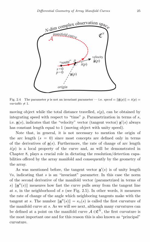
Fig. 2.4 The parameter p is not an invariant parameter — i.e. speed = ‖a(p)‖ = s(p) =variable = 1.
moving object while the total distance travelled, s(p), can be obtained byintegrating speed with respect to “time” p. Parametrization in terms of s,i.e. a(s), indicates that the “velocity” vector (tangent vector) a′(s) alwayshas constant length equal to 1 (moving object with unity speed).
Note that, in general, it is not necessary to mention the origin ofthe arc length (s = 0) since most concepts are defined only in termsof the derivatives of a(s). Furthermore, the rate of change of arc lengths(p) is a local property of the curve and, as will be demonstrated inChapter 8, plays a crucial role in dictating the resolution/detection capa-bilities offered by the array manifold and consequently by the geometry ofthe array.
As was mentioned before, the tangent vector a′(s) is of unity length∀s, indicating that s is an “invariant” parameter. In this case the normof the second derivative of the manifold vector (parametrized in terms ofs) ‖a′′(s)‖ measures how fast the curve pulls away from the tangent lineat s, in the neighborhood of s (see Fig. 2.5). In other words, it measuresthe rate of change of the angle which neighboring tangents make with thetangent at s. The number ‖a′′(s)‖ = κ1(s) is called the first curvature ofthe manifold curve at s. As we will see next, although many curvatures canbe defined at a point on the manifold curve A ∈CN , the first curvature isthe most important one and for this reason this is also known as “principal”curvature.

July 6, 2004 9:29 WSPC/Book Trim Size for 9in x 6in chap02
26 Differential Geometry in Array Processing
Fig. 2.5 How fast the curve pulls away from the tangent line, at point s, is measuredby a′′(s) with ‖a′′(s)‖ = κ1(s).
2.2 Curvatures and Coordinate Vectors in CN
We have seen that the arc length s is the invariant parameter of a manifoldcurve of an array of N sensors. With the array manifold curve embedded inan N -dimensional complex space (or equivalently in a 2N real space) andparametrized in terms of the arc length s, it is essential to attach/defineto the running point a = a(s) on the curve a number of curvatures as wellas a continuous differential and orthonormal system of coordinates u1(s),u2(s), . . . , u2N (s).
2.2.1 Number of Curvatures and Symmetricityin Linear Arrays
The curvatures of a space curve are of immense value in differential geom-etry as, according to the fundamental uniqueness theorem of [2, 17], cur-vatures uniquely define a space curve expressed in terms of arc length s,except its position in space.
For an array of N sensors (i.e. the manifold vector a(s) ∈ CN may bedescribed by 2N real components), at most 2N − 1 manifold curvaturescan be defined. However, if the array has some symmetrical sensors withrespect to the array centroid, then the manifold curve is situated wholly

July 6, 2004 9:29 WSPC/Book Trim Size for 9in x 6in chap02
Differential Geometry of Array Manifold Curves 27
in some subspace of dimensionality d (within the 2N dimensional space).Therefore, in this case up to d − 1 non-zero curvatures can be defined. Inparticular, if m denotes the number of sensors in symmetrical pairs then d
is given as follows:
d =
2N − m if sensor at the array centroid2N − m − 1 otherwise
(2.8)
This implies that 0 ≤ m ≤ N and according to m, linear sensor arrays aredivided into the following broad categories:
(1) Symmetric: m = N , i.e. all the sensors occur in symmetric pairs aboutthe origin.
(2) Non-Symmetric: m < N(a) Partially symmetric: 0 < m < N , i.e. at least one sensor has a
symmetric counterpart about the origin;(b) Fully asymmetric: m = 0, i.e. no sensor has a symmetrical coun-
terpart about the origin.
Note that a sensor at the origin is taken to be a symmetrical sensor.A representative example from each category is illustrated in Figs. 2.6, 2.7and 2.8.
Fig. 2.6 A symmetric linear array of N = 5 elements (m = 5, d = 2N − m − 1 = 4).
Fig. 2.7 A partially symmetric linear array of N = 5 elements (m = 2, d = 2N−m = 8).
Fig. 2.8 An asymmetric linear array of N = 4 elements (m = 0, d = 2N − m = 8).

July 6, 2004 9:29 WSPC/Book Trim Size for 9in x 6in chap02
28 Differential Geometry in Array Processing
2.2.2 “Moving Frame” and Frame Matrix
In the previous section we have seen that to the running point a(s) on thecurve A we attach a frame of orthonormal vectors u1(s), u2(s), . . . , u2N (s)together with d − 1 non-zero curvatures κ1(s), . . . , κd−1(s) with N − 1 ≤d ≤ 2N .
By ignoring the coordinate vectors with indices greater than d (thosecorresponding to zero curvatures) a frame of d orthonormal vectors u1(s),u2(s), . . . , ud(s), can be defined and attached to the running point a(s) onthe manifold curve, making a(s) the “origin” of the new coordinate system.This set of coordinate vectors, known as a “moving frame” (see Fig. 2.9),forms the matrix
U(s) = [u1(s), u2(s), . . . , ud(s)] ∈ CN×d (2.9)
and is derived from a fixed known frame U(0), (i.e. at s = 0 say) by rotation,using the transformation matrix F(s) ∈ Cd×d, i.e.
U(s) = U(0) · F(s) where F(0) = Id (2.10)
The matrix F(s) is a continuous differential real transformation matrixcalled frame matrix. This is a non-singular matrix with its main propertieslisted in Table 2.1.
Fig. 2.9 “Moving frame” U(0) and U(s).

July 6, 2004 9:29 WSPC/Book Trim Size for 9in x 6in chap02
Differential Geometry of Array Manifold Curves 29
Table 2.1 Properties of the frame matrix F(s).
1st property F(s) ∈ Rd×d
2nd property det(F(s)) = 1
3rd property F−1(s) = FT (s)
4th property FT (s) · F(s) = Id
5th property eleij(F) = (−1)i+jeleji(F)
6th propertyd∑
i=2even
eleii(F) = Tr(F)−ε2 where ε =
0 if d even1 if d odd
To summarize, the d×d real matrix F(s) is known as the “frame matrix”while the set of coordinates represented by the N × d complex matrix U(s)is the “moving frame.”
2.2.3 Frame Matrix and Curvatures
The question is, how the frame matrix F(s), at the running point s, isrelated to the curvatures of the manifold attached to this point. The initialpart of the mechanism to answer this question is to define the coordinatevectors in CN by exploiting and extending the procedure used in real spaceswhere a basis of up to N orthonormal vectors is necessary to fully define acurve in RN [17]. This extension, which provides the d coordinate vectors inCN blended with the curvatures, is summarized in a structured formationin Table 2.2.
Now let us focus on the (i + 1)th row of Table 2.2. That is,
ui+1(s) =u′
i(s) + κi−1.ui−1(s)κi
(2.11)
By solving Eq. (2.11) with respect to u′i(s), it is obvious that the differen-
tiation of the ith coordinate vector, for i 2, can be written as
u′i(s) = κi(s)ui+1(s) − κi−1(s)ui−1(s) for i 2 (2.12)
withu′
1(s) = a′′(s) = κ1(s)u2(s)
Note that the coordinate vectors are normalized to unity length.Equation (2.12) which can be rewritten in a more compact form as
U′(s) = U(s) C(s) (2.13)

July 6, 2004 9:29 WSPC/Book Trim Size for 9in x 6in chap02
30 Differential Geometry in Array Processing
Table 2.2 Estimation procedure of coordinate vectors and curvatures ofa curve A.
Coordinate Vector Curvature
1st u1(s) a′(s) κ1(s) =∥∥u′
1(s)∥∥
2nd u2(s) = 1κ1
u′1(s) κ2(s) = ‖u′
2(s) + κ1u1(s)‖
3rd u3(s) =u′2(s) + κ1u1(s)
κ2κ3(s) = ‖u′
3(s) + κ2u2(s)‖. . . . . . . . .. . . . . . . . .
ith ui(s) =u′
i−1(s) + κi−2.ui−2(s)
κi−1κi(s) = ‖u′
i(s) + κi−1.ui−1(s)‖
(i+1)th ui+1(s) =u′
i(s) + κi−1.ui−1(s)
κiκi+1(s) = ‖u′
i+1(s) + κi.ui(s)‖. . . . . . . . .. . . . . . . . .
dth ud(s) =u′
d−1(s) + κd−2.ud−2(s)
κd−1κd(s) = 0
where U′(s) = [u′1(s), u
′2(s), . . . , u
′d(s)] ∈ CN×d, d is the dimensionality of
the subspace in which the curve is embedded. The matrix C(s) ∈ Cd×d istermed the Cartan matrix, which is a real skew-symmetric matrix of thecurvatures defined as follows:
C(s)
0, −κ1(s), 0, . . . , 0, 0κ1(s), 0, −κ2(s), . . . , 0, 0
0, κ2(s), 0, . . . , 0, 0...
......
. . ....
...0, 0, 0, . . . , 0, −κd−1(s)0, 0, 0, . . . , κd−1(s), 0
(2.14)
Starting with Eq. (2.13) and then using Eq. (2.10), we have
U′(s) = U(s) C(s)
⇒ (U(0) F(s))′ = U(0) F(s) C(s)
⇒ U(0) F′(s) = U(0) F(s) C(s)
leading to the following expression
F′(s) = F(s) C(s) (2.15)

July 6, 2004 9:29 WSPC/Book Trim Size for 9in x 6in chap02
Differential Geometry of Array Manifold Curves 31
This is a first order differential equation of the frame matrix F(s) withinitial condition F(0) = Id. Therefore, its solution is
F(s) = expm(s C(s)) (2.16)
where expm(·) denotes the matrix exponential. Equation (2.16) provides therelationship between the frame matrix F(s) at the running point s and thecurvatures (Cartan matrix) of the manifold attached to this point, whichcan also be used to rewrite Eq. (2.10) as follows:
U(s) = U(0) expm(s C(s)) (2.17)
Finally, Eq. (2.15) implies that the Cartan matrix can always be writtenas a function of the frame matrix F(s) as follows
C(s) = F−1(s) F′(s) = FT (s) F′(s) (2.18)
where the 3rd property of F(s) given in Table 2.1 has been used. Rememberthat the Cartan matrix, as a formation of the curvatures, contains all theinformation about the local behavior and shape of the manifold curve.
2.2.4 Narrow and Wide Sense Orthogonality
As stated previously, for a general array manifold curve it is essential toattach, to a running point on the curve, a continuously differentiable andorthonormal system of coordinates U(s). The orthonormality of this contin-uously differentiable “moving” frame relies on the vector continuum ui(s)with constant magnitude and being orthogonal to its tangent. That is,
ui(s) ⊥ u′i(s), i.e. ui(s)
Hu′i(s) = 0
This, however, is only true for the broad class of arrays which are symmetricwith respect to their centroid, in which case m = N . In general, if the arrayis nonsymmetric (m < N), then the orthogonality is not valid although thecomplex vectors ui(s) have constant (unity) magnitude. In particular, theinner product of a complex vector of constant norm with its derivative ispurely imaginary, i.e.
uHi (s)u′
i(s) = imaginary (2.19)
This leads us to define orthogonality of two complex vectors of unitymagnitude as being “wide-sense” and “narrow-sense” orthogonality,

July 6, 2004 9:29 WSPC/Book Trim Size for 9in x 6in chap02
32 Differential Geometry in Array Processing
as follows:
Definition 2.1 Wide sense and narrow sense orthogonality of two com-plex vectors of unity magnitude:
“wide” sense orthogonality: Re(uHi (s).uj(s)) = 0, for i = j (2.20)
“narrow” sense orthogonality: uHi (s) · uj(s) = 0, for i = j (2.21)
Thus, for a general linear array, that is, for a non-symmetric array, thewide-sense orthogonality should be used, i.e.
Re(UH(s) · U(s)) = Id (2.22)
This, of course, is simplified to narrow-sense orthogonality UH(s)·U(s) = Id
for symmetrical arrays.Using the “wide sense” orthogonality for a general linear array, and
starting with Eq. (2.18), we get
Re(UH(s) · U′(s)) = C(s) (2.23)
Indeed
C(s) = FT (s) · F′(s) = FT (s) · Id · F′(s) = FT (s) · Re(UH(0) · U(0))︸ ︷︷ ︸=Id
· F′(s)
= Re
FT (s) · UH(0)︸ ︷︷ ︸=UH(s)
· U(0)F′(s)︸ ︷︷ ︸=U′(s)
= Re(UH(s)U′(s))
Furthermore, as it is shown in Appendix 2.7.1, the ith derivative of themanifold vector with respect to the arc length s (denoted by a′(i)(s)) isrelated to the coordinate vector in a simple way as follows:
Re((
a′(i)(s))H
· ui(s))
= κ1(s) · κ2(s) · · ·κi−1(s)
=i−1∏=1
κ(s) (2.24)
Based on Eq. (2.24), it is easy to prove that the determinant of the N × N
matrix formed by the first N derivatives of the manifold vector is related

July 6, 2004 9:29 WSPC/Book Trim Size for 9in x 6in chap02
Differential Geometry of Array Manifold Curves 33
to the curvatures by
|det[a′(s),a′′(s), . . . ,a′(N)(s)]|
= κN−11 (s) · κN−2
2 (s) · · ·κ2N−2(s) · κN−1(s)
=N−1∏=1
κN− (s) (2.25)
2.3 “Hyperhelical” Manifold Curves
In this section, the shape of the array manifold of a linear array of N
isotropic sensors is investigated using the theory developed in the previoussection. The manifold is parametrized in terms of a directional parameterp with the sensor locations given by the vector r in half-wavelengths. Thetheory is valid for any regular parametrized differential manifold curve Adefined as follows:
A a(p) ∈ CN , ∀p : p ∈ Ωp (2.26)
wherea(p) = exp(−j(πr cos p + v)) (2.27)
where r and v are two constant vectors and p is a generic parameter(parameter of interest). The main results are presented in the form of twotheorems but, firstly, it is easy to show using Eq. (2.3) that the arc lengths(p), and rate of change of arc length s(p), are given by the following expres-sions respectively:
s(p) = π ‖r‖ (1 − cos p) i.e. p(s) = cos−1(
1 − s
π‖r‖)
(2.28)
ands(p) = π‖r‖ sin p (2.29)
where the initial condition s(0) = 0 has been assumed.It is worth noting that for a linear array of N sensors with locations
r (in units of half-wavelengths) the rate of change of the arc length isa non-linear function of the directional parameter p and depends on thenorm of the vector of sensor locations. From Eq. (2.29), it can be furtherdeduced that for a small directional increment ∆p | p2 − p1|, the cor-responding change in arc length, to a first order approximation, can be

July 6, 2004 9:29 WSPC/Book Trim Size for 9in x 6in chap02
34 Differential Geometry in Array Processing
calculated as:
∆s = |s(p2) − s(p1)| (2.30)
= π‖r‖|cosp2 − cos p1| (2.31)
≈ π‖r‖∆p sin p; for small ∆p (2.32)
where p (p1 + p2)/2. This expression reveals crucial properties of thearray manifold of a linear array and provides considerable insight into itsresolving power. Consider a linear array and two impinging emitters witha directional separation of ∆p. It can easily be seen from Eq. (2.32) thatthe distance (arclength ∆s) between the corresponding manifold (response)vectors in CN is maximum when the emitters are at broadside and minimumwhen they are at endfire. Furthermore, if a larger array is employed, thenthe corresponding manifold vectors are further apart in CN . These factsare demonstrated by the variations of the rate of change of arc lengthwith azimuth for 5-sensor and 7-sensor standard ULAs of half-wavelengthspacings, plotted in Fig. 2.10.
Fig. 2.10 Variations of s(θ) for ULAs of 5 and 7 sensors.

July 6, 2004 9:29 WSPC/Book Trim Size for 9in x 6in chap02
Differential Geometry of Array Manifold Curves 35
This explains the better resolution of sources at broadside and the betterresolving power of the 7-sensor standard ULA, as evidenced by Fig. 2.10.It can therefore be concluded that the rate of change of arc length of thearray manifold plays a prominent role in determining the resolving powerof the array, as will be further detailed in Chapter 8.
Another important parameter of the array manifold curve is its totallength,
lm s(π) = 2π ‖r‖ (2.33)
which clearly increases in direct proportion to the sensor spacings. As can beseen, the manifold length depends on the number of sensors and their posi-tions. The manifold length is expected to influence the ambiguity propertiesof a linear array since it is obvious that longer manifolds are more prone to“spurious” parameters/results (manifold vectors that can be expressed aslinear combinations of other manifold vectors) unless the arrays are care-fully designed.
The array manifold can now be parametrized in terms of its arc lengthas follows:
A = a(s) ∈ CN , ∀s : s ∈ [0, lm] (2.34)where
a(s) exp(j(rs − πr + v)) (2.35)
andr r
‖r‖ (2.36)
is the vector of “normalized” sensor positions.From Eq. (2.35), and bearing in mind that the coordinate vectors are of
unit length, the following expressions for the first three manifold curvatures,for instance, may be derived from the first three rows of Table 2.2
u1(s) a′(s) = jr a(s)
u2(s) =1κ1
u′1(s) = − 1
κ1r2 a(s)
u3(s) =1κ2
(u′2(s) + κ1u1(s)) = − j
κ1κ2(r3 − κ2
1r) a(s)(2.37)
κ1(s) = ‖u′1(s)‖ = ‖r2‖
κ2(s) = ‖u′2(s) + κ1u1(s)‖ =
1κ1
‖r3 − κ21r‖
κ3(s) = ‖u′3(s) + κ2u2(s)‖ =
1κ1κ2
‖r4 − (κ21 + κ2
2)r2‖

July 6, 2004 9:29 WSPC/Book Trim Size for 9in x 6in chap02
36 Differential Geometry in Array Processing
In general, it can be shown that the ith coordinate vector and curvatureof the manifold of a linear array of isotropic sensors can be calculatedaccording to the following theorem.
Theorem 2.1 Hyperhelical Manifolds: The manifold of any lineararray of N omnidirectional sensors with locations given by r,
(a) is a curve of hyperhelical shape lying on a complex N -dimensionalsphere with radius
√N.
(b) The coordinate vectors and curvatures of this hyperhelix depend on thelower order curvatures, the number of sensors and their relative spacingand can be estimated by the following recursive equations:
ui (s) =(j)i
κ1κ2 · · ·κi−1
fix( i−12 )+1∑
n=1
(−1)n−1 bi−1,n ri−2n+2 a(s) (2.38)
κi =1
κ1κ2 · · ·κi−1
∥∥∥∥∥∥fix( i
2 )+1∑n=1
(−1)n−1 bi,n ri−2n+3
∥∥∥∥∥∥ (2.39)
where r = r
‖r‖ (normalized sensor positions)
κ1 = ||r2||κi−1 = 0
sum(r) = 0 (i.e. phase reference = array centroid)
Furthermore, the coefficients bi,n are given by:
bi,n =i−2n+3∑m1=1
i−2n+5∑m2=2+m1
· · ·i−1∑
mn−1=2+mn−2
κ2m1
κ2m2
· · ·κ2mn−1
; i, n > 2
(2.40)with
bi,1 = 1; i 1
bi,n =i−1∑m=1
κ2m i > 1
or recursively by
bi,n = bi−1,n + κ2i−1bi−2,n−1, i > 2, n > 1 (2.41)

July 6, 2004 9:29 WSPC/Book Trim Size for 9in x 6in chap02
Differential Geometry of Array Manifold Curves 37
with the initial conditions:bi,1 = 1, i ≥ 1
b2,2 = κ21
(2.42)
Corollary 2.1 The manifolds of uniform linear arrays are hypercirculararcs (closed hyperhelices).
The proof of the above theorem can be found in Appendix 2.7.2(page 54). Note that for notational convenience the second condition (row)of Eq. (2.8) may be ignored by redefining d 2N − m with N ≤ d ≤ 2N .This implies that in the special case of an array with a sensor at the arraycentroid, we attach to the running point a(s) on the curve A a movingframe of u1(s), u2(s), ..., ud(s) together with d−2 non-zero curvatures andone zero curvature (κd−1 (s) = 0). In this special case Eq. (2.38) cannot beused to calculate the dth coordinate vector ud(s) since the curvature κd−1
vanishes. Using an orthogonalization procedure, the (N × 1) vector ud(s)can be shown to be given by
ud(s) = [ 0, . . . , 0, 1, 0, . . . , 0 ]T (2.43)
where the non-zero entry is in the same position as the sensor at the centroidin the vector of sensor locations r.
2.3.1 Coordinate Vectors and Array Symmetricity
A close examination of Eq. (2.39) of Theorem 2.1, reveals some importantproperties of the manifold of a linear array of isotropic sensors. In particular,unlike the real case, the coordinate vectors of the linear array manifold curveembedded in CN are not in general mutually orthogonal. For example:
uH1 (s)u2(s) =
j
κ11T
N r3
uH1 (s)u3(s) = 0
uH2 (s)u3(s) =
j
κ2
(1κ2
11T
N r5 − 1TN r3
)uH
2 (s)u4(s) = 0
(2.44)
It can, however, be seen that some of the coordinate vectors (somecolumns of matrix U(s)) are mutually orthogonal. Indeed, it can be shownthat the odd-indexed coordinate vectors forming the matrix
Uodd(s) =[u1(s), u3(s), u5 (s), . . . , udodd
(s)]
(2.45)

July 6, 2004 9:29 WSPC/Book Trim Size for 9in x 6in chap02
38 Differential Geometry in Array Processing
are mutually orthogonal and that the same holds for the even-indexed coor-dinate vectors forming the matrix
Ueven(s) =[u2(s), u4(s), u6(s), . . . , udeven
(s)]
(2.46)
where deven = fix(d2 ) and dodd = fix(d−1
2 ) + 1. This can be expressed in acompact form as
UHodd(s)Uodd(s) = Idodd
UHeven(s)Ueven(s) = Ideven
(2.47)
withUH
odd(s)Ueven(s) = Ododd×deven
ReUHodd(s)Ueven(s) = Ododd×deven
(2.48)
Note also that, at broadside (i.e. p = 90), Uodd(s) is an imaginary matrixwhile Ueven(s) is a real matrix. In addition, in the special case of “symmetricarrays”, the coordinate vectors form a mutually orthogonal frame
symmetric arrays: UH(s)U(s) = IN ; (2.49)
since the sum of odd powers of the sensor locations is equal to zero.
2.3.2 Evaluating the Curvatures of Uniform Linear ArrayManifolds
The manifold curvatures (and hence the Cartan matrix C) of a linear arrayof isotropic sensors are constant, or equivalently, independent of parameterss or p. They depend, however, on the relative rather than the absolutesensor spacings. For instance, the manifold of a 3-element linear array withintersensor spacings 1.5 and 1 has the same curvatures with a 3-elementlinear array with spacings 0.75 and 0.5 (where the spacings are measuredin half wavelengths) but the length of its manifold is twice as long.
Using Theorem 2.1, all the curvatures of any linear array can be cal-culated. For instance, in Table 2.3, the first eight curvatures are tabulatedfor arrays with 3 to 10 elements chosen from the popular class of uniformlinear arrays with half-wavelength spacing. Furthermore, in Fig. 2.11 thefirst four curvatures are shown versus the number of elements in the array.It is apparent from Fig. 2.11 that the curvatures are monotically decreasingas the number of elements exceeds twice the order of the curvature.
In Fig. 2.12, the curvatures of a 13-element uniform linear array ofsensors are seen to follow a fading oscillating pattern.

July 6, 2004 9:29 WSPC/Book Trim Size for 9in x 6in chap02
Differential Geometry of Array Manifold Curves 39
It is important to point out that, because the manifold has constantprincipal (first) curvature and lies on a sphere with radius
√N , a lower
limit for κ1 is
κ1 >1√N
(2.50)
Table 2.3 The first eight curvatures of the manifold of uniform linear arrays.
N = 3 N = 4 N = 5 N = 6 N = 7 N = 8 N = 9 N = 10
‖r‖ 1.4142 2.2361 3.1623 4.1833 5.2915 6.4807 7.7460 9.0830κ1 0.7071 0.6403 0.5801 0.5372 0.5000 0.4693 0.4435 0.4214κ2 0 0.1874 0.2058 0.2047 0.1984 0.1908 0.1832 0.1760κ3 — 0.2343 0.3430 0.3603 0.3568 0.3469 0.3352 0.3234κ4 — 0 0 0.1489 0.1783 0.1880 0.1899 0.1884κ5 — — — 0.1323 0.2270 0.2554 0.2647 0.2660κ6 — — — 0 0 0.1201 0.1502 0.1637κ7 — — — — — 0.0895 0.1694 0.1002κ8 — — — — — 0 0 0.0664
Fig. 2.11 Curvatures of uniform linear arrays as functions of the number of sensors N .

July 6, 2004 9:29 WSPC/Book Trim Size for 9in x 6in chap02
40 Differential Geometry in Array Processing
Fig. 2.12 Curvatures of uniform linear array of 13 sensors with half-wavelengthintersensor spacing.
The above relation also stems from the following inner product aHu2in conjunction with the expression
(aHu1)′ = a′Hu1 + aHu′
1
⇒ (aHu1)′ = u H
1 u1 + aHu′1
⇒ aHu′1 = (aHu1)
′ − u H1 u1
That is,
aHu2 =1κ1
aHu′1 =
1κ1
((aHu1)
′ − u H1 u1
)=
1κ1
(0 − 1) = − 1κ1
⇒ ‖a‖︸︷︷︸=
√N
.‖u2‖︸︷︷︸=1
>1κ1
⇒ κ1 >1√N
Finally, it should be noted that the manifolds of non-omnidirectional lin-ear arrays are not hyperhelices. The first curvature of the manifold of

July 6, 2004 9:29 WSPC/Book Trim Size for 9in x 6in chap02
Differential Geometry of Array Manifold Curves 41
such arrays depends both on the relative spacing and the first two deriva-tives of each elemental pattern γk(p). In the case of the manifold of a4-element uniform linear array with non-isotropic, but identical, sensorswith directional pattern γk(p) = cos p, the variation of the first curvaturewith the azimuth direction is shown in Fig. 2.13. The constant first curva-ture of the corresponding isotropic array is also shown in the same figure.It is seen that there exist two bearings where the first curvature becomesequal to zero. From the variation of the first curvature, it is possible todeduce the geometrical object to which the manifold best fits. In the caseconsidered, it is apparent that the effect of the sinusoidal elemental patternis to deform the hyperhelix to a geometrical figure resembling an “eight”with a double point at the origin of the coordinates of CN .
2.4 The Manifold Length and Number of Windings(or Half Windings)
It is noted that the manifolds of uniform linear arrays with an odd numberof sensors and half-wavelength spacing consist of one winding (round) sincethe manifold vectors corresponding to the manifold boundaries coincide(i.e. a(0) = a(180)). In addition, the manifolds of uniform linear arrayswith an even number of sensors and half wavelength spacing, consist of onehalf winding (half round) since the manifold vectors corresponding to themanifold boundaries are opposite (i.e. a(0) = −a(180)). This situationhas forced the separation of a hyperhelix corresponding to a general arraywith an odd number of sensors into consecutive equal arcs of one windingand a hyperhelix corresponding to an array with an even number of sensorsinto consecutive equal arcs of half-winding.
The following theorem is concerned with the estimation of the numberof windings (N odd) and the number of half windings (N even) existing inthe manifold of an arbitrary linear array.
Theorem 2.2 Windings of a Hyperhelix: The number of windings(N odd), or the number of half windings (N even), of the hyperhelix ofEq. (2.26) is
nw =
manifold length=lm︷ ︸︸ ︷2π ‖r‖
lw(2.51)

July 6, 2004 9:29 WSPC/Book Trim Size for 9in x 6in chap02
42 Differential Geometry in Array Processing
Fig. 2.13 The principal curvature as a function of azimuth (top) and its polar repre-sentation (κ, p) (bottom) for a 4-element ULA of directional sensors — γk(p) = cos p.

July 6, 2004 9:29 WSPC/Book Trim Size for 9in x 6in chap02
Differential Geometry of Array Manifold Curves 43
where lw is the positive number that corresponds to the (N − 1)th root ofthe function
ξw(s) = Tr C expm(s C) (2.52)
with C denoting the Cartan matrix.
The independence of the curvatures from the absolute spacings (andhence the independence of the winding length from the absolute spacings)in conjunction with the dependence of the manifold length on the absolutespacings, reveals that two linear arrays with sensors at positions given bythe vectors r(1) and r(2) with r(1) = qr(2), where q is a scalar constant,
• have manifolds that fit upon each other, and• the associated number of windings (or half windings) satisfy the following
relationship
n(1)w
n(2)w
= q (2.53)
It is worth noting that the definition of half winding is restricted tolinear arrays with an even number of sensors and
a(0) = a(lw)U(0) = U(lw)F(0) = Id = F(lw)
⇒ Tr(F(0)) = Tr(F(lw)) = d
where lw represents the arc length of half winding. For an array with anodd number of sensors, the function ξw (Eq. (2.52)) does not generally havea root at the point on the manifold that corresponds to half the length ofone manifold winding.
Similarly, the definition of one winding is restricted to linear arrays withan odd number of sensors and
a(0) = −a(lw)U(0) = −U(lw)F(0) = Id = −F(lw)
⇒ Tr(F(0)) = −Tr(F(lw)) = d
where lw represents the arc length of one winding. For an array with aneven number of sensors, the function ξw does not generally have a rootat the point on the manifold that corresponds to twice the length of a

July 6, 2004 9:29 WSPC/Book Trim Size for 9in x 6in chap02
44 Differential Geometry in Array Processing
Fig. 2.14 Tr(F(s)) and ξw(s), given by Eq. (2.52), for a 5-element and a 6-element ULAof half wavelength spacing. Note that A1 = 5 = A2 and B1 = 6 = −B2.

July 6, 2004 9:29 WSPC/Book Trim Size for 9in x 6in chap02
Differential Geometry of Array Manifold Curves 45
half-manifold winding. Figure 2.14 provides a representative example fortwo arrays − with even and odd number of sensors.
2.5 The Concept of “Inclination” of the Manifold
In the previous section it has been shown that the shape of the manifoldof a general linear array of omnidirectional sensors is a complex circularhyperhelix lying on the complex N -dimensional sphere with radius
√N . In
this section, an attempt is made to identify the orientation of the arraymanifold (hyperhelix) on the complex N -dimensional space. Therefore, it isnecessary to establish a measure of the orientation of the manifold curve inCNusing the concept of array inclination angle. This is intuitively definedas follows:
Definition 2.2 Inclination Angle: The inclination angle ζinc of themanifold of a linear array is the angle formed between any manifold vectora(s) and the subspace L [Usub(s)], i.e. the subspace spanned by the columnsof the matrix
Usub(s) [u2(s), u4(s), u6(s), . . . , uuptoN (s)
],
that is,ζinc = (a(s), L [Usub(s)])
or equivalently
cos ζinc =
√1N
aH(s) PUsuba(s) (2.54)
where PUsub is the projection operator onto L [Usub(s)].
Having defined the matrix Usub(s) as a submatrix of Ueven(s) andbecause of the orthonormality of columns of the matrix Ueven(s) (seeEq. (2.47)) it is apparent that Eq. (2.54) can be rewritten as follows:
cos ζinc =
√√√√ 1N
N∑i=even
|aH(s) ui(s)|2 (2.55)
It is intuitively expected that the inclination angle should increase withthe degree of non-symmetry of the array, at least in the neighborhoodin which the array is nearly symmetrical. This can, in fact, be verifiedfrom Fig. 2.15 in which the inclination of the manifolds for a number of

July 6, 2004 9:29 WSPC/Book Trim Size for 9in x 6in chap02
46 Differential Geometry in Array Processing
Fig. 2.15 Inclination angle for a number of linear arrays with 4 and 6 sensors.
different arrays resulting from uniform linear arrays with 4 and 6 elements,of half-wavelength spacing, by varying the rightmost (leftmost) spacingfrom 0.5 half-wavelengths to 3 half-wavelengths is shown.
2.6 The Manifold-Radii Vector
Equation (2.55) shows that the inclination angle is directly related to theinner products of a manifold vector aH(s) with the coordinate vectors u2,u4, u6, . . . , etc. This demonstrates that the relationship between aH(s) andits associated coordinate vectors ui(s),∀i is very important.
For example, the relationships between aH(s) and the first four coordi-nate vectors, at a point, are:
aH(s)u1(s) = j1TN r
aH(s)u2(s) = − 1κ1
aH(s)u3(s) =j
κ1κ2
(1T
N r3 − κ211
TN r)
aH(s)u4(s) = − κ2
κ1κ3
(2.56)

July 6, 2004 9:29 WSPC/Book Trim Size for 9in x 6in chap02
Differential Geometry of Array Manifold Curves 47
It is easy to see that the orthogonality between a manifold vector andthe corresponding tangent vector u1(s) at every point is guaranteed if thephase reference is taken at the array centroid so that
sum (r) = 0 or, equivalent, 1TN r = 0 (2.57)
If the array is also symmetric, then at every point along the manifold, thecorresponding response vector is orthogonal to the odd-indexed coordinatevectors.
To provide a more general expression of the inner product
aH(s)ui(s); ∀i
the following definition is essential.
Definition 2.3 Manifold-Radii Vector: For an N sensor linear arraywith m sensors in symmetrical pairs the vector
R =
[0,−R2, 0, −R4, 0, . . . , 0, −Rd]T
if sensor at the array centroid
[0,−R2, 0, −R4, 0, . . . , 0, −Rd−1, 1]T
otherwise
(2.58)
is defined as the array manifold-radii vector having elements the manifoldradii Ri (for i = even) with
R2 =1κ1
and Ri =∏i−2
n=even κn∏i−1n=odd κn
for i > 2 (2.59)
Lemma 2.1 The inner product aH(s)ui(s), ∀i: For a linear array ofN sensors the inner products of a manifold vector a(s) with its d coor-dinate vectors ui(s) are constant and given by the following expressions:
aH(s)ui(s) = −Ri for i even (2.60)
Re(aH(s)ui(s)) =
0 for i = d and odd1 for i = d and odd
or, in a more compact form, as
aH(s)Ueven(s) = [−R2,−R4, . . . ,−Rdeven ] (2.61)
Re(aH(s)U(s)
)= RT

July 6, 2004 9:29 WSPC/Book Trim Size for 9in x 6in chap02
48 Differential Geometry in Array Processing
Note that the inner product of a manifold vector and the correspondingnormal vector (or second coordinate vector) is the negative of the radiusof curvature (i.e. −1/κ1) and hence the other interior products can beconsidered as higher order “manifold radii.” Using the above lemma theinclination angle of Eq. (2.55) can be rewritten as
ζinc = arccos(‖Rsub‖√
N
)= constant (2.62)
revealing that the inclination is constant, depending only on the norm of asub-vector of the manifold radii vector and the number of sensors, whereRsub is the vector formed by the first N elements of vector R.
Definition 2.4 Dual arrays: The dual array of a linear array, non-symmetrical with respect to the array centroid, is the array with sensorshaving positions given by rdual
i = −rN-i+1 for i = 1, . . . , N .
Using the above definition it can be seen that, although the manifoldsof two dual arrays are not identical, they have the same curvatures andlength. Thus, apart from the fact that they have opposite inclinations, theyhave the same differential geometry properties.
Based on the above concepts the array manifold vector of Eq. (2.27) or(2.35) can be written as
a (s) = U (s) R = U (0) F(s)R where F(s) = expm (sC) (2.63)
or, by choosing the N coordinate vectors (i.e. N columns of U(0)) at s = 0to be the standard orthonormal basis in RN , i.e. setting U(0) = IN , andexpressing s as a function of p using Eq. (2.28),
a (p) = expm (π ‖r‖ (1 − cos p) C) R (2.64)
where p = 0 (s = 0) is taken along the array axis. Equation (2.64) isassociated with a real N -dimensional hyperhelix having the same lengthand identical curvatures with those of the complex N -dimensional manifoldand this is formally described below.
Theorem 2.3 Real N-dimensional Hyperhelix of SymmetricLinear Arrays: For a symmetric linear array of N sensors with loca-tions r, manifold radii vector R and Cartan matrix C, there is areal N -dimensional hyperhelix described as the locus of the following

July 6, 2004 9:29 WSPC/Book Trim Size for 9in x 6in chap02
Differential Geometry of Array Manifold Curves 49
real vector
areal(p) = expm(π‖r‖(1 − cos p) C)R ∈ RN (2.65)
having differential geometry properties equivalent to those of the complexN -dimensional manifold of the array.
The vector areal(p) can be regarded as the real representation of themanifold of a symmetric array in RN .
Thus, the manifolds of symmetrical arrays are shown to admit real rep-resentation. This can be seen intuitively from the fact that the compo-nents of a manifold vector of symmetrical arrays exist in conjugate pairs.In addition, in the absence of weighting, such arrays have purely real arraypatterns.
Example 2.1 3-element linear array: The real N -dimensional curvehaving the same differential geometry properties as the manifold of a 3-element uniform linear array, is a circle. In fact, for N = 3, Eq. (2.65)of Theorem 2.3 takes a closed analytical form. The second curvature κ2
vanishes and the Cartan and Frame matrices are expressed as
C =
0, −κ1, 0κ1, 0, 00, 0, 0
(2.66)
F(s) = expm(s C) =
cos(κ1s), sin(κ1s), 0− sin(κ1s), cos(κ1s), 0
0, 0, 1
(2.67)
In addition, the vector R is
R =[0, − 1
κ1, 1
]T
(2.68)
By applying Eq. (2.65) of Theorem 2.3, the real curve with the samedifferential geometry properties with the manifold of a 3-element uniformlinear array, is given by the real vector continuum
areal(s) =[− 1
κ1sin (κ1s) ,
1κ1
cos(κ1s), 1]T
(2.69)
or, as a function of p,
areal(p) =[− 1
κ1sin (κ1π ‖r‖ (1 − cos p)) ,
1κ1
cos (κ1π ‖r‖ (1 − cos p)) , 1]T

July 6, 2004 9:29 WSPC/Book Trim Size for 9in x 6in chap02
50 Differential Geometry in Array Processing
while the conventional complex array manifold vector of this array is
a(p) =[exp (jπ ‖r‖ cos p) , 1, exp (−jπ ‖r‖ cos p)
]T(2.70)
It is clear that Eq. (2.69) is the equation of a closed circle (assuming half-wavelength spacing) with radius 1/κ1 for −‖r‖π ≤ s ≤ ‖r‖π. If the twospacings of the above array become unequal, κ2 does not vanish and themanifold becomes a helix.
Example 2.2 MUSIC Algorithm: To test the proposed results andexpressions as well as to demonstrate their use in a DF problem, the MUSICalgorithm is employed, expressed in terms of the curvatures and coordinatevectors. Indeed, if Pn is the projection operator on to the noise subspacespanned by the noise-level eigenvectors of the array covariance matrix, thecost function of MUSIC can be expressed as a function of the differentialgeometry parameters of the array manifold as follows:
ξMUSIC(s) = aH(s)Pna(s)
= RT FT (s)UH(0)︸ ︷︷ ︸=aH(s)
PnU(0)F(s)R︸ ︷︷ ︸a(s)
= Tr
UH(0)PnU(0)︸ ︷︷ ︸=Pn
v(s)︷ ︸︸ ︷F(s)R
=vT (s)︷ ︸︸ ︷RT F(s)︸ ︷︷ ︸
=V(s)
= Tr
(PnV(s)
)(2.71)
The matrix Pn is a constant d × d Hermitian matrix correspondingto a transformation of the second-order statistics of the data collectedand is termed the orientation of the noise subspace. The matrix V(s) isa real d × d symmetric matrix depending exclusively on the curvaturesand acts as a differential geometry operator on the suitably transformeddata. If the array is symmetric it is apparent that the same expressionholds but the matrices V(s) and Pn are N × N dimensional real matri-ces and v(s) = areal(s). Hence, there is a significant reduction in thedimensionality.
In Fig. 2.16, the differential geometry version of MUSIC is simulatedfor a seven element uniform linear array which operates in the presence ofsignals with directions of arrival 35, 120, and 125. This figure illustratesthat the proper estimation of the three sources is possible by expressing the

July 6, 2004 9:29 WSPC/Book Trim Size for 9in x 6in chap02
Differential Geometry of Array Manifold Curves 51
Fig. 2.16 MUSIC spectrum based on Eq. (2.71) for a ULA of 7 sensors operating in thepresence of 3 emitting sources.
MUSIC cost function in terms of the differential geometry properties of themanifold.
Deductions
(1) Setting ‖a(s)‖ =√
N and using the wide sense orthonormality of thecoordinate vectors, the following relation is derived
‖expm(s C)R‖ =√
N (2.72)
By setting s = 0, it is obvious that
‖R‖ =√
N (2.73)
(2) If Rsub is the vector formed by the first N components of the manifoldradii vector, then
‖Rsub‖ ≤ ‖R‖ =√
N (2.74)
However, for symmetrical arrays, Rsub = R, therefore,
symmetric arrays: ‖Rsub‖ =√
N (2.75)

July 6, 2004 9:29 WSPC/Book Trim Size for 9in x 6in chap02
52 Differential Geometry in Array Processing
From the above it can be deduced that, for any symmetric sequence ofN real numbers ri, Eq. (2.65) gives an expression for a real hyperhelix(on a real N -dimensional sphere with radius
√N) of latitude
latitude =
π
2− arccos
(1√N
)N odd
0 N even
and with curvatures given by Eq. (2.39), Theorem 2.1.(3) All 3-element non-symmetrical linear arrays have a constant inclination
angle of 35.26. Also, the first curvature of all 3-element linear arraysis 0.707 so that, in the non-uniform case, i.e. non-symmetrical case,‖Rsub‖ =
√2.
(4) The manifold of arrays with symmetry with respect to their centroid donot exhibit inclination, which is equivalent to saying that these mani-folds “stand upright” or, in other words, that they admit a representa-tion entirely in RN .
Finally the Frobenius norm of the Cartan matrix (i.e. ‖C‖F ) is relatedto the array symmetricity as follows:
(i) ‖C‖F = 1 if array = symmetric(ii) ‖C‖F =
√2 if array = fully asymmetric
(iii) 1 < ‖C‖F <√
2 if array = partially symmetric(2.76)
and, at this point, it is convenient to summarize the special properties ofthe manifolds of symmetric linear arrays:
Symmetric Linear Arrays of N Sensors
• sum(rn) = 0, for n odd
• m = N (with d= 2N − m = N)
• (No. of κi = 0) =
N − 1 if sensor at the array centroidN − 2 otherwise
• inclination angle: ζinc = 0
• UH(s)U(s) = IN (narrow sense orthogonality)• aH(s)U(s) = RT
• Rsub = R
• areal (p) = expm(π ‖r‖ (1 − cos p) C) R ∈ RN
(2.77)

July 6, 2004 9:29 WSPC/Book Trim Size for 9in x 6in chap02
Differential Geometry of Array Manifold Curves 53
2.7 Appendices
2.7.1 Proof of Eq. (2.24)
The proof will be done by induction. For i = 2, we have
a′′(s)Hu2(s) = κ1u2(s)H︸ ︷︷ ︸
a′′(s)H
u2(s) = κ1(s) (2.78)
Assuming that
Rea′(i−1)(s)Hui−1(s)
= κ1(s)κ2(s) · · ·κi−2(s) (2.79)
we have to prove that
Rea′(i)(s)Hui(s)
= κ1(s)κ2(s) · · ·κi−1(s) (2.80)
For convenience let us drop the parameter s. The argument of the first partof Eq. (2.80) can be written as follows:
(a′(i))Hui
= (a′(i−1))′Hui
=((a′(i−1))Hui
)′− (a′(i−1))Hu′
i
=((a′(i−1))Hui
)′− (a′(i−1))H(κiui+1 − κi−1ui−1)︸ ︷︷ ︸
=u′i (see Eq. (2.12))
=((a′(i−1))Hui
)′− κi(a′(i−1))Hui+1 + κi−1(a′(i−1))Hui−1︸ ︷︷ ︸
=κ1κ2···κi−2
(2.81)
However, by using the fact that the vectors a′(i−1) can be expressed as alinear combination of coordinate vectors with no higher order than (i − 1),Eq. (2.81) can be rewritten as follows:
(2.81) =
i−1∑
j=1
cjuj
H
ui︸ ︷︷ ︸imaginary
′
− κi
i−1∑j=1
cjuj
H
ui+1︸ ︷︷ ︸imaginary
+ κ1κ2 · · ·κi−2κi−1
(2.82)

July 6, 2004 9:29 WSPC/Book Trim Size for 9in x 6in chap02
54 Differential Geometry in Array Processing
where cj are scalar coefficients. Then, by taking the real part of both sidesand using the property that
ReuHj ui = 0 for j = i (2.83)
we have
Re(
a′(i))H
ui
= 0 + 0 + κ1κ2 · · ·κi−2κi−1 (2.84)
and this completes the proof.
2.7.2 Proof of Theorem 2.1
Consider a manifold vector described by the following equation:
a a(p) = exp(−j(πr cos p + v)) (2.85)
The magnitude of the manifold tangent vector is
‖a(p)‖ = ‖jπ sin p r a ‖ = π sin p‖r‖ = s(p) (2.86)
Hence the length of the manifold is
lm s(π) =∫ π
0‖a(p)‖ dp = 2π ‖r‖ (2.87)
The first coordinate vector is merely the tangent given by
u1(s) = a′(s) =dads
=dadp
dp
ds
= (jπ sin pr a)︸ ︷︷ ︸=a(p)
· (π sin p ‖r‖)︸ ︷︷ ︸=s(p)
−1
= jr a (2.88)
It can be seen that, since the origin of the coordinates is at the arraycentroid,
aHu1(s) = 0 (2.89)
However, the derivative of u1(s) with respect to arc length s is
u′1(s) =
du1
dp
dp
ds
= (jr a)︸ ︷︷ ︸=u1
· (π sin p‖r‖)︸ ︷︷ ︸=s(p)
−1

July 6, 2004 9:29 WSPC/Book Trim Size for 9in x 6in chap02
Differential Geometry of Array Manifold Curves 55
= jr (jπ sin pr a)︸ ︷︷ ︸a
· 1π sin p‖r‖
= −r2 a (2.90)
Therefore, by using Table 2.2, the first curvature is estimated as
κ1 = ‖u′1(s)‖ = ‖r2‖ (2.91)
Next, the second coordinate vector is chosen to be
u2(s) =u′
1(s)‖u′
1(s)‖
= − 1κ1
r2 a (2.92)
Furthermore,
u′2(s) =
du2
dp
dp
ds
=(
− 1κ1
r2 a)
︸ ︷︷ ︸=u2
(π sin p ‖r‖)︸ ︷︷ ︸=s(p)
−1
= − 1κ1
r2 (jπ sin pr a)︸ ︷︷ ︸a
· 1π sin p‖r‖
= −j1κ1
r3 a (2.93)
and
u′2(s) + κ1u1(s) = −j
(1κ1
r3 − κ1r
) a (2.94)
Hence, the second curvature (see Table 2.2) and the third coordinatevector are
κ2 = ‖u′2(s) + κ1u1(s)‖
=1κ1
.‖ r3 − κ21 r‖ (2.95)

July 6, 2004 9:29 WSPC/Book Trim Size for 9in x 6in chap02
56 Differential Geometry in Array Processing
andu3(s) =
1κ2
(u′2(s) + κ1u1(s))
= −j1κ2
·(
1κ1
r3 − κ1r
) a
= −j1
κ1κ2· (r3 − κ2
1r) a (2.96)
In order to estimate the third curvature it is necessary to estimate theterms u′
3(s) and κ2u2(s). Indeed,
u′3(s) =
du3
dp
dp
ds
= −j1
κ1κ2· (r3 − κ2
1r) a︸ ︷︷ ︸
=u3
· (π sin p‖r‖)︸ ︷︷ ︸=s(p)
−1
= −j1
κ1κ2· (r3 − κ2
1r) (jπ sin pr a)︸ ︷︷ ︸=a
(π sin p‖r‖)−1
=1
κ1κ2· (r4 − κ2
1r2) a (2.97)
and
κ2u2(s) = −κ2
κ1r2 a (2.98)
which implies
u′3(s) + κ2u2(s) =
1κ1κ2
(r4 − (κ2
1 + κ22)r
2) a (2.99)
By taking the magnitude of the above equation the third curvature isestimated as
κ3 = ‖u′3(s) + κ2u2(s)‖
=1
κ1κ2‖r4 − (κ2
1 + κ22)r
2‖ (2.100)
and, thus, the fourth coordinate vector is
u4(s) =1κ3
(u′3(s) + κ2u2(s))
=1
κ1κ2κ3
(r4 − (κ2
1 + κ22)r
2) a (2.101)

July 6, 2004 9:29 WSPC/Book Trim Size for 9in x 6in chap02
Differential Geometry of Array Manifold Curves 57
By continuing in the same way as above, it can be shown that
(i) the fourth curvature, for N > 4, is
κ4 = ‖u′4(s) + κ3u3(s)‖
=1
κ1κ2κ3
∥∥∥∥∥∥r5
−(κ21 + κ2
2 + κ23)r
3
+(κ1κ3)2 r
∥∥∥∥∥∥ (2.102)
so that the fifth coordinate vector is
u5(s) =1κ4
(u′4(s) + κ3u3(s))
= j1
κ1κ2κ3κ4
r5
−(κ21 + κ2
2 + κ23)r
3
+(κ1κ3)2 r
a (2.103)
(ii) the fifth curvature, for N > 5, is
κ5 = ‖u′5(s) + κ4u4(s)‖
=1
κ1κ2κ3κ4
∥∥∥∥∥∥∥∥r6
−(κ21 + κ2
2 + κ23 + κ2
4)r4
+(
(κ1κ3)2 + (κ1κ4)2
+(κ2κ4)2
)r2
∥∥∥∥∥∥∥∥ (2.104)
so that the sixth coordinate vector is
u6(s) =1κ5
(u′5(s) + κ4u4(s))
= − 1κ1κ2κ3κ4κ5
r6
−(κ21 + κ2
2 + κ23 + κ2
4)r4
+(
(κ1κ3)2 + (κ1κ4)2
+(κ2κ4)2
)r2
a
(2.105)
The above equations can be generalized for any index i, to give thecurvature κi and the vectors ui by the following expressions:
κi =1
κ1κ2 · · ·κi−1
∥∥∥∥∥ri+1 − ri−1 ·i−1∑n=1
κ2n + ri−3 ·
i−3∑n=1
i−1∑=n+2
(κnκ)2 − · · ·∥∥∥∥∥
(2.106)

July 6, 2004 9:29 WSPC/Book Trim Size for 9in x 6in chap02
58 Differential Geometry in Array Processing
or, equivalently,
κi =1
κ1κ2 · · ·κi−1
∥∥∥∥∥∥fix( i
2 )+1∑n=1
(−1)n−1 bi,n ri−2n+3
∥∥∥∥∥∥ (2.107)
and
ui(s) =(j)i
κ1κ2 · · ·κi−1
fix( i−12 )+1∑
n=1
(−1)n−1 bi−1,n ri−2n+2 a(s) (2.108)
where bi,n is given by Eq. (2.40).From Eq. (2.106), it can be seen that the terms inside the norm operator
form a polynomial of the sensor locations with coefficients given by the cur-vatures. This polynomial is expressed in a more compact form in Eq. (2.39).Furthermore, note that the numbers bi,n satisfying the recursive Eq. (2.41)can be easily proven by induction.

July 9, 2004 13:52 WSPC/Book Trim Size for 9in x 6in chap03
Chapter 3
Differential Geometry of ArrayManifold Surfaces
The locus of all array manifold vectors a(p, q) ∀(p, q) forms a surface knownas the array manifold. This is a two-parameter manifold embedded in anN -dimensional complex space and is formally defined as
M = a(p, q) ∈ CN , ∀(p, q) : p, q ∈ Ω (3.1)
where Ω denotes the parameter space. The shape of the surface is veryimportant. In the same way that the shape of a curve A is uniquelydefined by its curvatures, the shape of a two-parameter manifold (surface)may be quantitatively expressed in terms of intrinsic geometrical parame-ters such as the Gaussian curvature KG(p, q) of the surface (see Fig. 3.1)and the geodesic curvature κg(p, q) of the curves lying on the surface (seeFig. 3.2).
More specifically, for a point a a(p, q) on the manifold surface, theparameters of interest, intrinsic to the manifold surface, together with neces-sary building blocks of surface differential geometry, will be identified in thischapter and extended from three-dimensional real space to N -dimensionalcomplex space. In order to achieve this all the ramifications and subtletiesinvolved in this process have been taken into consideration.
Thus, it is first necessary to introduce the building blocks of surfacedifferential geometry such as the manifold metric, first fundamental coeffi-cients and the Christoffel symbols.
However, to proceed, it is essential to start with two definitions whichwill aid in the development of the basic theory. These are
• the definition of a constant parameter curve on M,• the “regularity” condition by defining the array manifold (surface) as a
“vector” function.
59
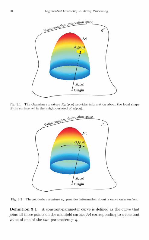
July 9, 2004 13:52 WSPC/Book Trim Size for 9in x 6in chap03
60 Differential Geometry in Array Processing
Fig. 3.1 The Gaussian curvature KG(p, q) provides information about the local shapeof the surface M in the neighbourhood of a(p, q).
Fig. 3.2 The geodesic curvature κg provides information about a curve on a surface.
Definition 3.1 A constant-parameter curve is defined as the curve thatjoins all those points on the manifold surface M corresponding to a constantvalue of one of the two parameters p, q.

July 9, 2004 13:52 WSPC/Book Trim Size for 9in x 6in chap03
Differential Geometry of Array Manifold Surfaces 61
Definition 3.2 A regular parametric representation of a surface M isdefined as a vector function
a = a(p, q) (3.2)
of parameters p and q in the parameter space Ω, if and only if ∀p, q ∈ Ω, thederivatives ap = da/dp and aq = da/dq exist, are continuous and non-zerowith
rank[ap, aq] = 2 (3.3)
The vectors ap and aq at a specific point A on the manifold representthe tangent vectors to the p- and q-parameter curves respectively passingthrough A and also form a basis for the tangent plane to the surface at thatpoint, i.e.
Tangent plane = L [T] where T = [ap, aq] ∈ CN×2 (3.4)
The regularity condition of Eq. (3.3) ensures that a tangent plane exists atall points on the surface. Note that the basis created by T is, in general,not orthonormal.
3.1 Manifold Metric
Let a = a(p, q) be the regular parametric representation of a surface Membedded in an N -dimensional complex space.
Then the (2 × 2) real semipositive definite symmetric matrix G,defined as
G ReTHT
=
‖ap‖2, ReaH
p aq
Re
aH
q ap
,
∥∥aq
∥∥2
=[gpp, gpq
gqp, gqq
](3.5)
is said to be the manifold metric. The elements gpp, gqq, and gpq (notegqp = gpq) of G are known, in Differential Geometry terms, as the firstfundamental coefficients (or metric coefficients) expressing the magnitudesand inner products of the parameter-curve tangent vectors and entirelydescribing the manifold properties of the surface. For instance, the anglebetween the two parameter curves of the surface at a point (p, q) can beexpressed as
(ap, aq
)= arccos
(gpq√gpp gqq
)(3.6)

July 9, 2004 13:52 WSPC/Book Trim Size for 9in x 6in chap03
62 Differential Geometry in Array Processing
The metric coefficients provide a way of measuring trajectories on non-Euclidean spaces through the use of weighting coefficients. For example, aninfinitesimal distance on the Euclidean plane is measured by
ds2 = dx2 + dy2 (3.7)
whereas on a general non-Euclidean surface it is given by
ds2 = gppdp2 + 2gpqdpdq + gqqdq2 (3.8)
It is also customary to use superscripts to denote the elements of theinverse matrix G−1
G−1 =[gpp gpq
gqp gqq
](3.9)
where clearly
gpp =gqq
det(G), gqq =
gpp
det(G), gpq = gqp =
−gpq
det(G)(3.10)
while the following properties may be easily proven:
(i) gpp, gqq ≥ 0(ii) det(G) ≥ 0 (by Schwarz’s inequality)(iii) gpp, gpq and gqq are variant under parameter transformation
(3.11)
Note that the metric G is, by construction, a semipositive definitematrix, i.e.
xT Gx 0, ∀x ∈ R2 (3.12)
which implies that at some points on the surface M this matrix can possiblybe singular in order to account for the fact that there may not exist aunique tangent space (L[T]) at each point. That is, at a point (p, q) witha non-unique tangent space, the matrix G is singular. These points are theboundaries of the manifold surface.
3.2 The First Fundamental Form
Again, let a = a(p, q) be the regular parametric representation of a manifoldsurface M embedded in N -dimensional complex space. Then the differentialmapping da = apdp + aqdq maps increments dp and dq on the (p, q)parameter plane on to vector apdp + aqdq on the tangent plane at a(p, q).

July 9, 2004 13:52 WSPC/Book Trim Size for 9in x 6in chap03
Differential Geometry of Array Manifold Surfaces 63
The scalar I, defined as
I = ‖da‖2 =∥∥apdp + aqdq
∥∥2 (3.13)
=[dp dq
]G
[dp
dq
]= dpT Gdp (3.14)
withdp =
[dp, dq
]Tis known as the first fundamental form and essentially represents the dis-tance between two neighboring points a(p, q) and a(p + dp, q + dq) on themanifold surface.
Two properties of I which may be readily established are
(i) I ≥ 0 with equality when dp = dq = 0(ii) I is invariant under a parameter transformation
(3.15)
The first fundamental form I is essential for the evaluation of lengthsof curves, and areas, on the manifold surface. For instance, let a(t) a(p(t), q(t)) with t1 ≤ t ≤ t2 be a regular curve lying on a surfacea = a(p, q). Then clearly the length of the curve is given by
length of curve =∫ t2
t1
∥∥∥∥dadt
∥∥∥∥ dt =∫ t2
t1
√I
dt2dt (3.16)
It may be similarly shown that the area of a segment W on the surface ofa manifold a = a(p, q) is given by
area of segment =∫∫W
√det(G) dp dq (3.17)
The significance of Eqs. (3.16) and (3.17) in relation to the intrinsicgeometry of a surface M will be clarified later on in this chapter. However,it is clear from Eq. (3.17) that
√det(G) dp dq describes an infinitesimally
small area on the manifold surface which is a function of (p, q) and thearray geometry r. Small uncertainties, or variations, in the sensor posi-tions will invariably result in small variations in the infinitesimal area√
det(G) dp dq on the manifold at point (p, q). The parameter√
det(G)can hence serve as a tool for detecting the changing shape of the manifoldsurface [18].

July 9, 2004 13:52 WSPC/Book Trim Size for 9in x 6in chap03
64 Differential Geometry in Array Processing
3.3 Christoffel Symbol Matrices
In order to investigate the differential geometry of a surface a(p, q), it isnecessary to determine how the non-orthonormal basis T of the tangentplane varies from point to point on the array manifold. This informationcan be expressed in terms of the Christoffel symbols of first kind.
By using the matrix T = [ap, aq] and its two derivatives Tp and Tq with
Tζ = dT/dζ = [apζ , aqζ ] with ζ = p or q (3.18)
the Christoffel symbols of first kind represent the inner products betweenthe tangent vectors ap, aq (columns of T) and their derivatives (columns ofTp and Tq), and are defined as
Γi,jk ReaH
i ajk
with i, j, k = p or q (3.19)
Thus there are eight Christoffel symbols of first kind forming the twoChristoffel matrices of the first kind Γ1p and Γ1q defined as follows:
Γ1ζ Re
TH Tζ
=[Γp,pζ Γp,qζ
Γq,pζ Γq,qζ
]with ζ = p or q (3.20)
where, due to the symmetry inherent in differentiation,
Γp,qp = Γp,pq and Γq,qp = Γq,pq. (3.21)
Although the differential geometry of a surface can be completely describedin terms of the above symbols, the process may be considerably simplifiedby the use of two other matrices Γ2p and Γ2q which are related to thesymbols of the first kind Γ1p and Γ1q, respectively, in the following way:
Γ2ζ G−1Γ1ζ =
[Γp
pζ Γpqζ
Γqpζ Γq
qζ
]with ζ = p or q (3.22)
These matrices are known as the Christoffel symbol matrices of secondkind and are used as a transformation which provides the infinitesimal vari-ation of the tangent plane as a point moves on the manifold surface, namely
dT = T(Γ2pdp + Γ2qdq) (3.23)
Once again, due to symmetry,
Γppq = Γp
qp and Γqpq = Γq
qp (3.24)

July 9, 2004 13:52 WSPC/Book Trim Size for 9in x 6in chap03
Differential Geometry of Array Manifold Surfaces 65
It is obvious that all Christoffel symbols are functions only of the firstfundamental coefficients gij (i, j = p, q) and their derivatives. Thus, forthis reason they play a central role in expressing the intrinsic geometry ofa surface, which is described in the next section.
3.4 Intrinsic Geometry of a Surface
Let us assume that
At a(t) ∈ CN , ∀t : t1 < t < t2 (3.25)
where
a(t) a(p(t), q(t)) (3.26)
denotes an arbitrary regular curve on a surface MM = a(p, q) ∈ CN , ∀(p, q) : p, q ∈ Ω (3.27)
where Ω denotes the parameter space.In order to define the intrinsic geometry of a surface, it is first necessary
to appreciate the concept of an isometric mapping.
Definition 3.3 Isometry: A one-to-one mapping of a surface M on toanother surface M is called an isometric mapping, or isometry, if the lengthof an arbitrary curve At on M is equal to the length of its image At on M,
where
At a(t) ∈ CK , ∀t : t1 < t < t2M a(p, q) ∈ CK , ∀(p, q) : p, q ∈ Ω
Hence we may think of isometry as the bending of a surface into adifferent shape without changing the distance (along the surface) betweenany of its points. Consequently, the “inhabitants” of such a surface wouldnot be aware of any change at all, as their geometric measurements remainexactly the same. The combination of the above definition with Eqs. (3.16)and (3.17) implies that:
Corollary 3.1 A one-to-one mapping of a surface M on to anothersurface M is an isometry if and only if at corresponding points a(p, q) anda(p, q) the first fundamental coefficients remain unchanged, i.e. gij = gij
∀i, j = p, q.
Thus, there is no difference in the measurement of lengths, angles, andareas on isometric surfaces although the surfaces, when viewed from the

July 9, 2004 13:52 WSPC/Book Trim Size for 9in x 6in chap03
66 Differential Geometry in Array Processing
embedding space, may have entirely different geometric shapes. An iso-metric mapping is by necessity both angle-preserving (conformal)and area-preserving (equiareal).
Definition 3.4 Intrinsic Property and Intrinsic Geometry: Aproperty of a surface which remains invariant under an isometry iscalled an intrinsic property of the surface. The totality of the intrin-sic properties of a surface is known as the intrinsic geometry of thesurface.
Naturally a property of a surface is an intrinsic property if it onlydepends on the first fundamental coefficients (and hence the magnitudesand inner products of the tangents to the surface). The intrinsic geometryof a surface is completely independent of the space in which the surface isembedded and is built from solely isometric invariants.
Next, two important features of intrinsic geometry are presented,namely:
• Gaussian curvature KG, and,• geodesic curvature κg.
3.4.1 Gaussian Curvature
By considering the surface as a whole body with intrinsic properties, Gauss,according to his “Theorema Egregium”, assigned to every point on thesurface a(p, q), independently of any specific curve passing through it, areal number KG called Gaussian curvature. Research into surfaces hasproduced several formulas for KG. For example, the Gaussian curvaturefor surfaces embedded in the 3-dimensional Euclidian space R3 is givenbelow (see [2]).
KG(p, q) =
(aT
p T)
·(aT
q T)
−(
d2adp dq
)T
T
det(G)(3.28)
where T T (p, q) is the unique normal to the surface at point (p, q).As the array manifold is embedded in CN (and not in R3) a unique
normal does not exist to each point and, therefore, Eq. (3.28) cannot bedefined for array manifolds. Here we will only consider the intrinsic for-mula for the Gaussian curvature which is independent of the normal space.For instance, an intrinsic formula for the Gaussian curvature, KG(p, q),of a surface, can be shown to be of the form [17] (also known as the

July 9, 2004 13:52 WSPC/Book Trim Size for 9in x 6in chap03
Differential Geometry of Array Manifold Surfaces 67
curvature scalar):
KG(p, q) =1
det(G)
12
(2d2gpq
dp dq− d2gpp
dq2 − d2gqq
dp2
)+
∑i,j=p,q
gij det
[Γi,pq Γi,pp
Γj,qq Γj,qp
] (3.29)
The above expression may be more compactly represented in terms of theChristoffel symbols:
KG(p, q) =1
det (G)
d
dpΓp,qq − d
dqΓp,qp
+ col2 Γ2pT col1 Γ1q− col2 Γ2qT col1 Γ1p
(3.30)
where colimatrix denotes the ith column of the matrix.Here the following intrinsic formula is used, adapted from [19], and
expressed as a function of the metric G as follows:
KG(p, q) = − 1√det(G)
d
(√det(G)gpp
Γqpq
)dp
−d
(√det(G)gpp
Γqpp
)dq
(3.31)
where Γqpq, Γq
pp are elements of the 2 × 2 real matrices Γ2p and Γ2q.The sign of the Gaussian curvature of Eq. (3.31) or (3.29), provides
an indication of the local shape of the surface in that neighborhood.For instance, the surface around a point (p, q) is locally:
• elliptic, if KG(p, q) > 0 (the whole neighborhood of the surface at thepoint considered lies on one side of the tangent hyperplane),
• hyperbolic, if KG(p, q) < 0 (one part of the surface at the point consideredlies on one side of the tangent hyperplane and the other part on the otherside),
• either parabolic or planar (i.e. flat), if KG(p, q) = 0 (there is a straightline of the surface, lying totally on the tangent space).
Example 3.1 The following lists a number of surfaces in R3 and theirrespective Gaussian curvatures:
(a) Sphere of radius R: KG = 1/R2 ⇒ Surface is elliptic at every point.(b) Cylinder or Cone: KG = 0 ⇒ Surface is parabolic at every point.(c) 2-D plane: KG = 0 ⇒ Surface is flat at every point.
July 9, 2004 13:52 WSPC/Book Trim Size for 9in x 6in chap03
68 Differential Geometry in Array Processing
If the Gaussian curvature at a point on the manifold is a positive num-ber, the local neighborhood of that point is equivalent to the local neigh-borhood of a point on a sphere of radius
√1/KG. Also note that surfaces
which have a constant Gaussian curvature at every point (e.g. Parts (b) and(c) of Example 3.1 above — a zero Gaussian curvature at every point) aresaid to be developable surfaces and will be discussed later in Section 3.5.
Apart from defining the local shape of a surface, the Gaussian curva-ture has important implications with regards to isometric mappings. Forexample,
two surfaces which are related by an isometric mapping musthave the same Gaussian curvature at corresponding points
(since KG is an intrinsic property)
The converse of this is in general not true. However if two surfaces havethe same constant Gaussian curvature, then any two sufficiently smallneighborhoods of the surfaces are related by an isometric mapping. Inparticular
• if KG(p, q) = constant, ∀(p, q) then, using Minding’s theorem [19] whichstates that two surfaces of the same constant curvature are locallyisometric, we have the following cases:
(1) if KG = 0, the surface M is isometric with the plane,(2) if KG > 0, the surface M is isometric with a sphere of radius
1/√
KG, and(3) if KG < 0, the surface M is isometric with a surface of revolution,
called a pseudo-sphere, determined by the value 1/√−KG.
As a result, developable surfaces for which KG = 0 are the only surfacesthat can be mapped isometrically onto a plane. This feature will be usedlater in Section 3.5.
3.4.2 Curves on a Manifold Surface: Geodesic Curvature
The Gaussian curvature, discussed in the previous section, and the geodesiccurvatures are the two most important parameters of the intrinsic geometryof a surface. This means that these two parameters remain invariant underan “isometry” (see Corollary 3.1, page 65).
In this section we will focus our attention on geodesic curvature κg(s)which is the final differential geometry parameter of interest to be presentedin this study, and is associated with curves lying on the manifold surface.However, initially the arc length of a curve on the manifold surface should

July 9, 2004 13:52 WSPC/Book Trim Size for 9in x 6in chap03
Differential Geometry of Array Manifold Surfaces 69
be defined and then, in order to understand the significance of κg(s), thegeodecity concept should be introduced.
3.4.2.1 Arc Length
The arc length s can be interpreted in physical terms as the total distancecovered by a person travelling along a certain path on a certain landscape.For a curve At
At a(t) ∈ CN , ∀t : t ∈ Ωt (3.32)
wherea(t) a(p(t), q(t))
on the array manifold surface M, the arc length s is the total distancetravelled along the curve At from an “initial” point (p(t1), q(t1)) to the“current” point (p(t2), q(t2)) under consideration. Its expression as a func-tion of the manifold metric is, based on Eq. (3.16):
arc length(curve on a surface)
: s =∫ t2
t1
√dpdt
T
Gdpdt
dt (3.33)
where
p = [p(t), q(t)]T and, hence,dpdt
=[dp
dt,dq
dt
]T
(3.34)
3.4.2.2 The Concept of Geodicity
It is well known that the curve with the minimum length between twopoints in an Euclidian space is a straight line. This concept is extendedto a curve connecting two points on a surface and the curve of minimumlength belonging to the surface is called a geodesic curve (equivalent to astraight line in a plane). By considering a curve on a surface connectingtwo points, the closeness of this curve to a geodesic curve can be assessedby means of the geodesic curvature, κg, with κg = 0 corresponding to ageodesic curve. That is,
geodesic curve ⇐⇒ a curve with κg = 0 (3.35)
3.4.3 Geodesic Curvature
We have seen that geodesic curves on an arbitrary geometric surface gen-eralize the notion of a straight line in Euclidean geometry. It is also knownthat a straight line a(t) = x + ty is characterized by zero curvature or

July 9, 2004 13:52 WSPC/Book Trim Size for 9in x 6in chap03
70 Differential Geometry in Array Processing
acceleration κ1 = ‖a′′‖ = 0. Following this line of reasoning, the intrinsicacceleration, or geodesic curvature, of a curve is defined as follows:
Definition 3.5 Geodesic Curvature: The geodesic curvature κg of acurve a(t) on a surface M is equal to the component of the curve’s firstcurvature κ1 along the tangent plane to the surface at every point alongthe curve.
Clearly the geodesic curvature is a function of the first fundamentalcoefficients only and is consequently preserved under an isometric map-ping. This implies that an isometric mapping is by necessity also ageodesic mapping.
Following the above definition, we reach the same conclusion as that ofEq. (3.35), i.e.
a geodesic curve on a surface M may be defined as a curvewhose geodesic curvature is zero at every point along itslength
For example, since for a geodesic curve the direction of acceleration isalways orthogonal to the surface, the inhabitants of a surface perceive noacceleration at all — for them the geodesic is a “straight” line.
It can also be shown that in the neighborhood of a point A on a surface,there exists a unique geodesic through A in any given direction. Conse-quently a unique geodesic joins point A with every point B in its neighbor-hood. Furthermore, the geodesic defines a unique arc of minimum lengthbetween neighboring points A and B. The converse is also true in that ifa(t) is an arc of minimum length between any two points on a surface, a(t)is a geodesic.
The geodesic curvature can be estimated (for proof, see Appendix 3.7.1)by the following expression:
κg(s) =√
det (G) p′T[
0 1−1 0
](p′′ + (Γ2pp
′ + Γ2qq′) p′) (3.36)
where
p = [p(s), q(s)]T
where s is the arc length of the curve under consideration. From Eq. (3.36),a geodesic curve, i.e. a curve for which the geodesic curvature is invariably
July 9, 2004 13:52 WSPC/Book Trim Size for 9in x 6in chap03
Differential Geometry of Array Manifold Surfaces 71
zero, must satisfy the equation:
p′′ + (Γ2pp′ + Γ2qq
′) p′ = 02 ∀(p, q) (3.37)
Equation (3.37) is a system of two simultaneous equations which are thewell-known geodesic differential equations (page 64 [19]).
It is clear that the computation of both the Gaussian and geodesiccurvature parameters (see Eqs. (3.31) and (3.36)), involves the elements ofthe Christoffel Symbol matrices of second kind Γ2p and Γ2q.
It is also clear that the general expression for the geodesic curvatureκg of an arbitrary curve on a surface is rather involved but can be con-siderably simplified for the special case of constant-parameter curves [2]:Let us denote a “p-parameter curve” (or simply p-curve) on the surface Mcorresponding to a constant value of q = qo as
Ap|qo = a(p, qo) ∈ CN , ∀p : p ∈ Ωp, qo = constant (3.38)
and, in a similar fashion, a “q-parameter curve” (or simply q-curve) as
Aq|po = a(po, q) ∈ CN , ∀q : q ∈ Ωq, po = constant (3.39)
Different values of qo (or po, accordingly) generate a family of curves havingthe same properties covering the whole of the manifold surface M. Thus,there are two such families of curves providing two alternative ways oftreating the manifold surface. These are
• the family of p-parameter curves
M =Ap|qo , ∀qo : qo ∈ Ωq
(3.40)
• the family of q-parameter curves
M =Aq|po , ∀po : po ∈ Ωp
(3.41)
Both families of p- and q-curves can be used to describe the manifoldsurface M but different parametrizations of the surface provide families ofcurves with different properties.
Note that if two families of curves are orthogonal and one family consistsof geodesic curves, then these two families constitute a set of what is knownas “geodesic coordinates.”
Based on the above definitions and using Eq. (3.36), the geodesic cur-vature κg,p for p-curves (i.e. curves of constant parameter q = qo) of anarray manifold can be shown, using dq/ds = 0 and dp/ds = 1/
√gpp, to be

July 9, 2004 13:52 WSPC/Book Trim Size for 9in x 6in chap03
72 Differential Geometry in Array Processing
equal to
κg,p κg(p, qo) =
√det (G)
g3pp
Γqopp (3.42)
Similarly, for the q-curves (i.e. curves of constant parameter p = po), usingdp/ds = 0 and dq/ds = 1/
√gqq, the geodesic curvature κg,q can be found
to be
κg,q κg(po, q) = −√
det (G)g3
Γpoqq (3.43)
Thus an alternative approach is produced by treating the manifoldsurface as a family of curves which fully covers and describes the corre-sponding surface.
In this book (Chapters 4 and 5), two different array manifoldparametrizations, having significant differences, will be studied. Eachparametrization treats the same array manifold M, using two differentfamilies of curves with diverse properties. These are
• the (θ, φ) parametrization (or, azimuth-elevation parametrization),• the (α, β) parametrization (or, cone-angle parametrization).
3.5 The Concept of “Development”
In Section 3.4.1, we have seen that by examining the sign of the Gaussiancurvature KG of the array manifold it is possible to study its shape. It isrecognized that apart from the fact that the Gaussian curvature offers anindication about the manifold shape, its importance is enhanced by the factthat if it satisfies certain stringent conditions (valid for a very broad classof arrays) the geodesic mappings of the individual manifold curves result ina consistent mapping of the whole manifold on the parameter plane, calledthe development of the manifold (see Fig. 3.3), which is defined as follows:
Definition 3.6 Development: Let At be a differentiable curve lying onthe manifold M expressed in terms of a parameter t as follows:
At = a(t) a(p(t), q(t)) ∈ CN , ∀ζ : t ∈ Ωt (3.44)
Furthermore, let s(t) be the arc length along Atgiven by Eq. (3.33). The
development of Aton the plane R2 is the plane curve
Ad = ad(t) ∈ R2, ∀t : t ∈ Ωζ (3.45)

July 9, 2004 13:52 WSPC/Book Trim Size for 9in x 6in chap03
Differential Geometry of Array Manifold Surfaces 73
Fig. 3.3 The concept of “development.”
with curvature κd(t) and arc length sd(t) given by
κd(t) = κg(t) and sd(t) =∫
t
κ−1d (t) dt (3.46)
where
κg(t) κg((p(t), q(t))) = geodesic curvature of At
Thus, the curvature κd(t) of the development of a manifoldcurve A
t is the geodesic curvature of that curve. The motivationbehind the conservation of the geodesic curvatures is to maintain the char-acteristic that the shortest path between two points on the surface mapsto a straight line on the plane (i.e. the shortest path on the development),otherwise the development will represent a “distorted” surface.
The relation between the Gaussian curvature and the “development”is addressed by Beltrami’s theorem [20, 21]. This theorem states that if a

July 9, 2004 13:52 WSPC/Book Trim Size for 9in x 6in chap03
74 Differential Geometry in Array Processing
surface is mapped to another surface and the mapping is such that geodesiccurves in one surface are mapped onto geodesic curves in the other sur-face (geodesic mapping) then if one surface has a constant Gaussian cur-vature the other must also have a constant Gaussian curvature, in orderto have a distortionless mapping. Surfaces of constant KG are known as“developable” surfaces [17]. Thus the condition for the development1 toexist is KG to be constant ∀(p, q), since a manifold surface M with a vary-ing Gaussian curvature KG cannot be adequately mapped onto the plane.
3.6 Summary
In this chapter regularly parametrized differential surfaces, embedded inCN , which may represent the locus of array manifold vectors, have beenstudied in terms of two generic parameters p and q. Thus for a point a(p, q)on a manifold surface M in CN the main intrinsic geometry parametershave been presented with main emphasis given to
• the Gaussian curvature KG of M, and,• the geodesic curvature κg of a curve A lying on M.
Then a manifold surface was treated as a family of curves on the sur-face M. This treatment is very convenient as it permits a unified frameworkfor the analysis of the linear and non-linear array manifolds. Furthermore,to provide a simplified representation of the analysis, with many potentialbenefits, the class of developable surfaces has been identified and the con-cept of the development has been introduced. This concept will be employedin the next chapter to map the array manifold surface, embedded in a com-plex N -dimensional space, on to a real parameter plane whilst preserving itsmain intrinsic geometry properties and characteristics. This has potentialto simplify the analysis of array manifold surfaces.
3.7 Appendices
3.7.1 Proof of Eq. (3.36) — Geodesic Curvature
Consider the locus of the manifold vectors a(p, q), ∀(p, q), forming the sur-face M embedded in CN . Consider a curve A
A a(s) ∈ CN , ∀s : s ∈ Ωs (3.47)
1Note that the “development” is on a plane and planes have constant (equal to zero)Gaussian curvature.

July 9, 2004 13:52 WSPC/Book Trim Size for 9in x 6in chap03
Differential Geometry of Array Manifold Surfaces 75
wherea(s) a(p(s), q(s))
lying on M and let us define p(s) [p(s), q(s)]T where s is the arc lengthof the curve. Then the tangent vector at a point (p(s), q(s)) on the curveA is given as follows:
a′ ≡ da(s)ds
= T p′
where T = [ap, aq] ∈ CN×2 such that L[T] is the tangent space tothe manifold surface at (p(s), q(s)). Furthermore, let us define the matrixB = [b1, b2] ∈ CN×2 as an orthonormal basis for the space L[T] with b1chosen to be equal to a′/‖a′‖. This gives the expression:
B = [b1, b2] = TEpH (3.48)
where
Ep =1√
det (G)
√
det (G)gpp
− gpq√gpp
0 √gpp
∈ R2×2 (3.49)
is the Gram-Schmidt orthonormalization matrix, such that the first col-umn of TEp is the basis vector ap/‖ap‖ and the matrix H ∈ R2×2 is theorthogonal rotation matrix:
H =[cos ψ − sin ψ
sin ψ cos ψ
](3.50)
where ψ is the rotation angle between the tangent vector to the p-curve ap
and the tangent vector to the curve under consideration a′:
ψ = (ap,a
′) = arccos
(ReaH
p a′∥∥ap
∥∥ ‖a′‖
)(3.51)
By projecting the second derivative
a′′ d (a′)ds
=dT
ds
dpds
+ Td2pds2 (3.52)
of the manifold vector at (p(s), q(s)) onto the subspace L[B] (note thatL[B] = L[T]), we have
PBa′′ = κ1b1 + κgb2 (3.53)
July 9, 2004 13:52 WSPC/Book Trim Size for 9in x 6in chap03
76 Differential Geometry in Array Processing
where PB = B(BHB
)−1BH is the projection operator. The coefficient of b2,
that is κg, is defined as the geodesic curvature of the curve at (p(s), q(s)) andrepresents the component of a′′ in the direction of b2. Hence its expression is
κg = RebH2 a′′ (3.54)
The vector b = [0, 1]T will be used for notational purposes such thatb2 = Bb. Substituting the expressions of b2 and a′′ into Eq. (3.54) gives,after some manipulation:
κg(s) = bT HT ETp G
(Γ2p
dp
ds+ Γ2q
dq
ds
)dpds
+d2pds2
. (3.55)
In Eq. (3.55) the term bT HT ETp G can be simplified to
√det(G) · [−p′, q′],
providing
κg(s) =√
det (G)[−p′
q′
]T ((Γ2pp
′ + Γ2qq′) p′ + p′′) (3.56)

July 6, 2004 9:30 WSPC/Book Trim Size for 9in x 6in chap04
Chapter 4
Non-Linear Arrays:(θ, φ)-Parametrization of Array
Manifold Surfaces
It is common practice to express the direction of array signals in terms ofazimuth angle θ and elevation angle φ. In this case the response vector ofan array of N omnidirectional sensors is (see Eq. (1.22))
a (θ, φ) = exp(−jrT k (θ, φ)
)(4.1)
where r is the matrix with columns the sensor location and k(θ, φ) is thewavenumber vector given by Eq. (1.3). Thus by using the directional param-eters (θ, φ), instead of the generic parameters (p, q) of the previous chapter,the two-parameter array manifold M of Eq. (3.1) becomes
M = a(θ, φ) ∈ CN , ∀(θ, φ) : (θ, φ) ∈ Ω (4.2)
where
Ω = (θ, φ) : θ ∈ [0, 360) and φ ∈ [0, 90)
The aim of this chapter is to demonstrate the feasibility and potentialbenefits of the theoretical framework presented in Chapters 2 and 3 byexamining various non-linear arrays of omnidirectional sensors. However,in order to proceed, the following derivatives of the wavenumber vectork(θ, φ) are required
first derivatives:
kθ = π[− sin θ cos φ, cos θ cos φ, 0]T
kφ = π[− cos θ sin φ,− sin θ sin φ, cos φ]T(4.3)
second derivatives:
kθθ = π[− cos θ cos φ,− sin θ cos φ, 0]T
kθφ = −kθ tan φ
kφφ = −k(θ, φ)(4.4)
77

July 6, 2004 9:30 WSPC/Book Trim Size for 9in x 6in chap04
78 Differential Geometry in Array Processing
where the following notation has been used
kp =dk (θ, φ)
dpand kpq =
d2k(θ, φ)dp dq
(4.5)
with
(p and q) = (θ or φ)
4.1 Manifold Metric and Christoffel Symbols
For an azimuth-elevation array system of omnidirectional sensors the func-tion a = a(θ, φ),∀(θ, φ), provides a regular parametric representation ofthe manifold surface M. With M embedded in an N -dimensional complexspace, the manifold metric G is a function of the array geometry r andgiven by the following expression
G =[gθθ, gφθ
gθφ, gφφ
]= [kθ kφ]T rrT [kθ kφ] (4.6)
Thus, for arrays of omnidirectional sensors, the elements of the metric G
can be computed as
gpq = kT
p rrT kq where p and q = θ or φ (4.7)
while the Christoffel symbol matrices are
First kind:
Γ1θ =
=Γθ,θθ︷ ︸︸ ︷
kT
θ rrT kθθ,
=Γθ,φθ︷ ︸︸ ︷−gθθ tan φ
kT
φ rrT kθθ︸ ︷︷ ︸=Γφ,θθ
, −gθφ tan φ︸ ︷︷ ︸=Γφ,φθ
and
Γ1φ =
=Γθ,θφ︷ ︸︸ ︷
−gθθ tanφ,
=Γθ,φφ︷ ︸︸ ︷−kT rrT kθ
−gθφ tan φ︸ ︷︷ ︸=Γφ,θφ
, −kT rrT kφ︸ ︷︷ ︸=Γφ,φφ
(4.8)

July 6, 2004 9:30 WSPC/Book Trim Size for 9in x 6in chap04
Non-Linear Arrays: (θ, φ)-Parametrization of Array Manifold Surfaces 79
Second kind:
Γ2θ =
Γθ
θθ,
=Γθφθ︷ ︸︸ ︷
− tan φ
Γφθθ, 0︸︷︷︸
=Γφφθ
and
Γ2φ =
=Γθ
θφ︷ ︸︸ ︷− tanφ, Γθ
φφ
0︸︷︷︸=Γφ
θφ
, Γφφφ
(4.9)
It should be noted from Eq. (4.9) that Γφθφ = 0. This simplifies the
Gaussian curvature of Eq. (3.31), for a 3D array of N -omnidirectionalsensors, to
KG(θ, φ) =1√
det(G)d
dφ
(√det(G)gθθ
Γφθθ
)(4.10)
which, in general, is not constant and, as it can be easily proven, can-not be negative (i.e. KG(θ, φ) 0, ∀(θ, φ)). This leads to the followingtheorem.
Theorem 4.1 The manifold surface of an array of N -omnidirectionalsensors of arbitrary geometry is never hyperbolic. It is elliptic and embeddedin an N -dimensional complex space.
In Chapter 3 we have stated that surfaces of constant Gaussian cur-vature are known as “developable surfaces.” As KG(θ, φ) of Eq. (4.10)is in general positive or zero, but not constant ∀(θ, φ), the array man-ifold of omnidirectional sensors is not a developable surface. Therefore,the existence of the “development” (see Definition 3.6, page 72) is notguaranteed. However, for some array geometries, the Gaussian curvatureof Eq. (4.10) is constant. Array geometries which have been identified tosatisfy this condition include all planar arrays as well as a special class ofthree-dimensional (3D) arrays, known as 3D-grid arrays which are definedand discussed next.

July 6, 2004 9:30 WSPC/Book Trim Size for 9in x 6in chap04
80 Differential Geometry in Array Processing
4.2 3D-grid Arrays of Omnidirectional Sensors
Definition 4.1 — 3D-grid arrays.1 A three-dimensional array geometryof omnidirectional sensors is said to be a 3D-grid array if and only if thefollowing expression is satisfied:
rrT = ρ2I3 where ρ ∈ R (4.11)
Thus, in 3D-grid arrays the vectors rx, ry and rz are not only orthogonalbut also have the same magnitude. The following theorem is concernedwith the shape of the manifolds of 3D-grid arrays. To prove this theoremit suffices to show that these arrays have constant and positive Gaussiancurvature.
Theorem 4.2 The manifold surface of a 3D-grid array of N -omnidirectional sensors is spherical with radius πρ (and hence developable)embedded in an N -dimensional complex space.
Example 4.1 The 8-element cube array with all sides equal to one half-wavelength is a 3D-grid array and has a spherical manifold with Gaussiancurvature (2π)−1, or radius
√2π half-wavelengths.
Table 4.1 summarizes the results of the array manifold parameters for3D-grid arrays.
Table 4.1 Manifold parameters of 3D-grid arrays.
Intrinsic Parameter Expression
G(Eq. (3.5))
ρ2π2[cos2 φ, 0
0, 1
]det(G) ρ4π4 cos2 φ
Γ1θ(Eq. (3.20), (ζ=θ))
ρ2π2 cos φ sin φ
[0, −11, 0
]Γ1φ
(Eq. (3.20), (ζ=φ))ρ2π2 cos φ sin φ
[−1, 00, 0
]Γ2θ
(Eq. (3.22), (ζ=θ))
[0, − tan φ
cos φ sin φ, 0
]Γ2φ
(Eq. (3.22), (ζ=φ))
[− tan φ, 00, 0
]KG
(Eq. (3.31))
1ρ2π2
13D-grid arrays are also known as 3D balance symmetric arrays.

July 6, 2004 9:30 WSPC/Book Trim Size for 9in x 6in chap04
Non-Linear Arrays: (θ, φ)-Parametrization of Array Manifold Surfaces 81
4.3 Planar Arrays of Omnidirectional Sensors
A planar (2D) array can be seen as a special case of a 3D-array where allthe elements of the last (3rd) row of the matrix r are zeros (i.e. rz = 0N ).In this case, the term rrT has the following form[
L, 020T2 , 0
]where L =
[c1, c2
c2, c3
]∈ R2×2 (4.12)
Furthermore, if L = ρ2I2 with ρ ∈ R, the planar array is said to be a
2D-grid array (or 2D balance symmetric). Fig. 4.1 shows some examples of2D-grid array geometries.
Theorem 4.3 The Gaussian curvature KG of the two-parameter mani-fold of a planar array of N -omnidirectional sensors is constant at everypoint and equal to zero.
Proof. A proof of this theorem is given in Appendix 4.7.1.
Fig. 4.1 Examples of 2D-grid array geometries.

July 6, 2004 9:30 WSPC/Book Trim Size for 9in x 6in chap04
82 Differential Geometry in Array Processing
Fig. 4.2 Manifold Surface M of a Planar Array parametrized in terms of (θ,φ). This isa developable manifold-conoid generated by rotating a φ-curve (geodesic curve) aroundthe apex.
Thus according to Theorem 4.3, the Gaussian curvature KG of a planararray is identically zero (wherever defined). Hence, the manifold of a planararray is, what is called in differential geometry, flat or parabolic of conoidshape with the apex at point φ = ±90 (see Fig. 4.2). It is important tonote that the “flatness” does not imply that there exist straight lines, as inthe case of a surface in R3. It means that such surfaces can be generated byrotating a passing curve, which should have the special property of beinggeodesic, around an apex point. In this case the φ-curves are shown tocompose a family of geodesic curves passing from a singularity point, i.e.the apex of the developable manifold-conoid as illustrated in Fig. 4.2.
Furthermore, because KG never takes positive values, the manifold can-not be closed. According to Beltrami’s theorem, since KG is constant, themanifold is a developable surface. Based on the above discussion the fol-lowing theorem, concerned with the shape of the manifold of an array ofomnidirectional sensors, can be easily proven.
Theorem 4.4 The manifold surface of a planar array of N -omnidirectional sensors is a conoid lying on a hypersphere of radius
√N
embedded in an N -dimensional complex space.
Table 4.2 summarizes the results of the differential geometry parametersof planar arrays of omnidirectional sensors together with their correspond-ing simplified expressions for the case of 2D-grid arrays.

July 6, 2004 9:30 WSPC/Book Trim Size for 9in x 6in chap04
Non-Linear Arrays: (θ, φ)-Parametrization of Array Manifold Surfaces 83
Table 4.2 Manifold parameters of planar arrays.
Intrinsic Parameter 2D General Arrays 2D-grid Arrays
G(Eq. (3.5))
[gθθ, gφθ
gθφ, gφφ
]ρ2π2
[cos2 φ, 0
0, sin2 φ
]
det(G)π4
4det(L) sin2(2φ) ρ4π4 cos2 φ sin2 φ
Γ1θ(Eq. (3.20), (ζ=θ))
gθφ
tan φ, −gθθ tan φ
gφφ
tan φ, −gθφ tan φ
ρ2π2 cos φ sin φ
[0, −11, 0
]
Γ1φ(Eq. (3.20), (ζ=φ))
−gθθ tan φ,gθφ
tan φ
−gθφ tan φ,gφφ
tan φ
ρ2π2 cos φ sin φ
[−1, 00, 1
]
Γ2θ(Eq. (3.22), (ζ=θ))
[0, − tan φ1
tan φ, 0
] [0, − tan φ1
tan φ, 0
]
Γ2φ(Eq. (3.22), (ζ=φ))
[− tan φ, 0
0, 1tan φ
] [− tan φ, 0
0, 1tan φ
]
KG(Eq. (3.31))
0 0
Based on the results presented in Tables 4.1 and 4.2 a number of com-ments can be made. For instance, the Gaussian curvature of 3D-grid arraysis always positive and constant whereas for planar arrays it is always zero(constant). This implies that the array manifold of a 3D-grid array is iso-metric with a sphere of radius ρπ while the manifold of a planar array isisometric with a plane. In addition, for all 2D-grid and 3D-grid arrays, themanifold metric G is a diagonal matrix. The determinant of this matrix isgiven by the 2nd row of Tables 4.1 and 4.2 and can be easily proven for gridarrays. For planar arrays, the proof of det(G) = π4
4 det(L) sin2(2φ) is givenin Appendix 4.7.2. All these expressions indicate that the determinant ofthe manifold metric G is independent of the azimuth angle θ.
4.4 Families of θ- and φ-curves on the Manifold Surface
The array manifold can also be described and analyzed by treating thissurface as one of the following two families of curves:
(1) the family of θ-parameter curves defined as
Aθ|φo
, ∀φo : φo ∈ Ωφ (4.13)

July 6, 2004 9:30 WSPC/Book Trim Size for 9in x 6in chap04
84 Differential Geometry in Array Processing
where Aθ|φo
denotes the “θ-curve” on the surface M corresponding toa constant value of φ = φo represented as follows:
Aθ|φo
= a(θ, φo) ∈ CN , ∀θ : θ ∈ Ωθ, φo = constant (4.14)
(2) the family of φ-parameter curves defined in a similar fashion as
A
φ|θo, ∀θo : θo ∈ Ωθ
(4.15)
whereA
φ|θo= a(θo, φ) ∈ C
N , ∀φ : φ ∈ Ωφ, θo = constant (4.16)
with Ωθ [0
to 360) and Ωφ [0 to 90). Note that
M =A
θ|φo, ∀φo : φo ∈ Ωφ
=A
φ|θo, ∀θo : θo ∈ Ωθ
(4.17)
Figure 4.3 shows an illustrative representation of one “θ-curve” and one“φ-curve” lying on the array manifold surface M.
These two curves lying on M can be analyzed using the geodesic cur-vature. The geodesic curvature is one of the most important parametersof the intrinsic geometry of a surface. In particular this parameter is asso-ciated with curves lying on the surface and remains invariant under an“isometry.”
Fig. 4.3 An illustrative example of a θ-curve and a φ-curve on the manifold surface M.

July 6, 2004 9:30 WSPC/Book Trim Size for 9in x 6in chap04
Non-Linear Arrays: (θ, φ)-Parametrization of Array Manifold Surfaces 85
It can be proven that all 3D and all planar arrays have zero geodesiccurvature for the φ-curves. This implies that
κg,φ = 0 ⇐⇒ φ-curves = geodesic curves (4.18)
Furthermore, the geodesic curvature κg,θ for the θ-curves for 3D-grid and2D-grid arrays is constant (depending on φo) but is not zero. Hence
κg,θ = 0 ⇐⇒ θ-curves = geodesic curves (4.19)
while constant κg,θ implies that the development of the θ-curves of gridarrays are circles whose radius is a function of φo.
Using Eq. (3.42) it can be proven that for a general planar array thegeodesic curvature κg,θ is given as follows
κg,θ =
√det (G)
g3θθ
1tan φo
(4.20)
and this may not even be constant. The above results are summarized inTable 4.3.
Table 4.3 Geodesic curvature.
Curve κg 3D-grid Arrays Planar Arrays 2D-grid Arrays
Aθ|φo κg,θtan φo
ρπ
√det (G)
g3θθ
1tan φo
1ρπ cos φo
Aφ|θo(hyperhelix)
κg,φ 0 0 0
For the 2D-grid and 3D-grid arrays, the off-diagonal elements of themanifold metric G (i.e. gθφ, gφθ) are zero (see Tables 4.1, 4.2) and hencethe θ-curves and φ-curves are orthogonal and constitute geodesic coordi-nates i.e.
(θ-curves) ⊥ (φ-curves)(φ-curves) = geodesic curve
=⇒ geodesic coordinates (4.21)
Figure 4.4 shows an illustrative representation of a planar array manifoldsurface and its families of θ- and φ-curves as geodesic coordinates.
Theorem 4.5 The geodesic curves (φ-curves) on the manifold surfaceare complex hyperhelices embedded in CN .

July 6, 2004 9:30 WSPC/Book Trim Size for 9in x 6in chap04
86 Differential Geometry in Array Processing
Fig. 4.4 Families of θ-curves and φ-curves on the manifold M of a planar array.
Proof. Eq. (4.1), for constant θ (of value θ0), can be expressed as
a(θo, φ) = exp(−jπ(rx cos θo + ry sin θo) cos φ)
= exp(−jπr(θo) cos φ) (4.22)
wherer(θo) = rx cos θo + ry sin θo (4.23)
which matches Eq. (2.27) for r = r(θo), p = φ and v = 0. However,hyperhelical curves, such as φ-curves, have all their curvatures constant,independent of the parameters (θ, φ), as shown in Chapter 2.
Hence hyperhelical curves on the manifold surface M are not only ana-lytically “convenient” but also geodesic curves. Overall it may be concludedthat, although both families of curves can be used to describe the manifoldsurface M, the θ-curves are the more complicated of the two families.
Corollary 4.1 All members of the family of φ-curves of planar arrays areidentical apart from their length lm and position in complex N-dimensionalspace.
It is immediately apparent that
a(φ | θo) = a(φ | θo + 180) (4.24)
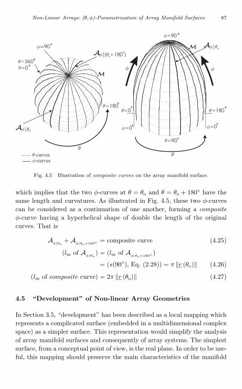
July 6, 2004 9:30 WSPC/Book Trim Size for 9in x 6in chap04
Non-Linear Arrays: (θ, φ)-Parametrization of Array Manifold Surfaces 87
Fig. 4.5 Illustration of composite curves on the array manifold surface.
which implies that the two φ-curves at θ = θo and θ = θo + 180 have thesame length and curvatures. As illustrated in Fig. 4.5, these two φ-curvescan be considered as a continuation of one another, forming a compositeφ-curve having a hyperhelical shape of double the length of the originalcurves. That is
Aφ|θo
+ Aφ|θo+180 = composite curve (4.25)
(lm of Aφ|θo
) = (lm of Aφ|θo+180 )
= (s(90), Eq. (2.28)) = π ‖r (θo)‖ (4.26)
(lm of composite curve) = 2π ‖r (θo)‖ (4.27)
4.5 “Development” of Non-linear Array Geometries
In Section 3.5, “development” has been described as a local mapping whichrepresents a complicated surface (embedded in a multidimensional complexspace) as a simpler surface. This representation would simplify the analysisof array manifold surfaces and consequently of array systems. The simplestsurface, from a conceptual point of view, is the real plane. In order to be use-ful, this mapping should preserve the main characteristics of the manifold

July 6, 2004 9:30 WSPC/Book Trim Size for 9in x 6in chap04
88 Differential Geometry in Array Processing
surface. For instance, a manifold surface with a varying Gaussian curva-ture cannot be adequately mapped onto a plane. Therefore KG should beconstant. Also, the transformation should map geodesic parameter curveson the manifold surface onto straight lines on the real plane which arethe geodesic curves of the plane (geodesic mapping). Based on the abovediscussion, such a mapping is provided below as a theorem.
Theorem 4.6 Consider an arbitrary point, (θ, φ), on the manifold sur-face of an array of N sensors. The image of the point (θ, φ) on the realparameter plane is given by
D(θ, φ) =
[x0(φ) +
∫ θ
0 κ−1g,θ(ϑ, φ) cos(ϑ)dϑ
y0(φ) +∫ θ
0 κ−1g,θ(ϑ, φ) sin(ϑ)dϑ
]∈ R2 (4.28)
where κg,θ(θ, φ) is the geodesic curvature of the θ-curves on the manifoldand x0(φ) and y0(φ) ∈ R are the integration constants such that:
x0 = − 12
∫ π
0 κ−1g,θ(ϑ, φ) cos(ϑ)dϑ and y0 = − 1
2
∫ π
0 κ−1g,θ(ϑ, φ) sin(ϑ)dϑ
The locus of the images D(θ, φ) ∀(θ, φ) is said to be the development2 ofthe manifold and has the following properties:
(i) It exists if and only if the Gaussian curvature of the manifold surfaceis constant.
(ii) The arc length sd(θ, φo) of θ-curves on the development is given by
sd(θ, φo) =∫
p
κ−1g,θ(ϑ, φo) dϑ (4.29)
(iii) The curvature of the θ-curves on the development is equal to thegeodesic curvature κg,θ(θ, φo) of the θ-curves on the manifold surface.
Proof. The proof is given in Appendix 4.7.3.
Note that the expressions for the integration constants assume the prop-erty κg,θ(θ, φo) = κg,θ(θ + π, φo) (which is generally valid), and have theeffect of shifting the curves to a common centre, i.e.
D(θ, φ) + D(θ + π, φ) = 0 (4.30)
The first condition of the theorem (i.e. KG = constant) is valid for 3D-gridand all planar arrays, which implies that these arrays are “developable,”with their “development” expressions summarized in Table 4.4.
2More on “development” and “developables” can be found in [17].
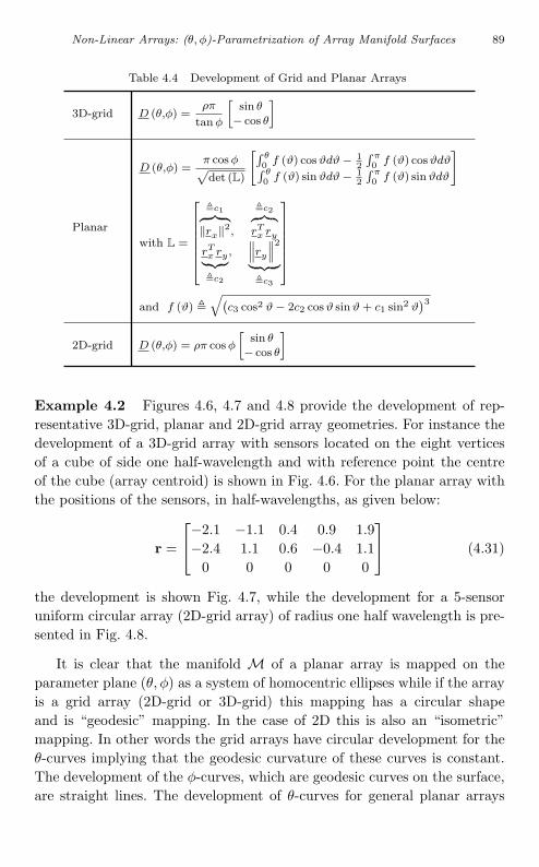
July 6, 2004 9:30 WSPC/Book Trim Size for 9in x 6in chap04
Non-Linear Arrays: (θ, φ)-Parametrization of Array Manifold Surfaces 89
Table 4.4 Development of Grid and Planar Arrays
3D-grid D (θ,φ) =ρπ
tan φ
[sin θ
− cos θ
]
Planar
D (θ,φ) =π cos φ√det (L)
[∫ θ0 f (ϑ) cos ϑdϑ − 1
2
∫ π0 f (ϑ) cos ϑdϑ∫ θ
0 f (ϑ) sin ϑdϑ − 12
∫ π0 f (ϑ) sin ϑdϑ
]
with L =
c1︷ ︸︸ ︷‖rx‖2,
c2︷ ︸︸ ︷rT
x ry
rTx ry︸ ︷︷ ︸c2
,∥∥∥ry
∥∥∥2︸ ︷︷ ︸c3
and f (ϑ)
√(c3 cos2 ϑ − 2c2 cos ϑ sin ϑ + c1 sin2 ϑ
)32D-grid D (θ,φ) = ρπ cos φ
[sin θ
− cos θ
]
Example 4.2 Figures 4.6, 4.7 and 4.8 provide the development of rep-resentative 3D-grid, planar and 2D-grid array geometries. For instance thedevelopment of a 3D-grid array with sensors located on the eight verticesof a cube of side one half-wavelength and with reference point the centreof the cube (array centroid) is shown in Fig. 4.6. For the planar array withthe positions of the sensors, in half-wavelengths, as given below:
r =
−2.1 −1.1 0.4 0.9 1.9−2.4 1.1 0.6 −0.4 1.1
0 0 0 0 0
(4.31)
the development is shown Fig. 4.7, while the development for a 5-sensoruniform circular array (2D-grid array) of radius one half wavelength is pre-sented in Fig. 4.8.
It is clear that the manifold M of a planar array is mapped on theparameter plane (θ, φ) as a system of homocentric ellipses while if the arrayis a grid array (2D-grid or 3D-grid) this mapping has a circular shapeand is “geodesic” mapping. In the case of 2D this is also an “isometric”mapping. In other words the grid arrays have circular development for theθ-curves implying that the geodesic curvature of these curves is constant.The development of the φ-curves, which are geodesic curves on the surface,are straight lines. The development of θ-curves for general planar arrays

July 6, 2004 9:30 WSPC/Book Trim Size for 9in x 6in chap04
90 Differential Geometry in Array Processing
Fig. 4.6 θ-curves and φ-curves development of the manifold of a 3D-grid array withsensors located on the eight vertices of a cube of side one half-wavelength and withreference point the centre of the cube (array centroid).
have an ellipsoidal shape with the two main axes at angles ψ0 and ψ0 +π/2with respect to the x-axis where:
ψ0 =12
tan−1(
2c2
c1 − c3
)(4.32)
with ci denoting the elements of the matrix L, i.e. L =[
c1, c2c2, c3
]. Indeed the
angle ψ0 can be found by examining the points of extremum curvatures.Since the curvature of the development is equal to κgθ, the geodesic cur-vature of the θ-curves of the planar array manifold is differentiated withrespect to θ and equated to zero:
dκgθ
dθ= 0 (4.33)
⇔ d(c3 cos2 ψ0 − 2c2 cos ψ0 sin ψ0 + c1 sin2 ψ0)−3/2
dψ0= 0

July 6, 2004 9:30 WSPC/Book Trim Size for 9in x 6in chap04
Non-Linear Arrays: (θ, φ)-Parametrization of Array Manifold Surfaces 91
Fig. 4.7 θ-curves and φ-curves development of the manifold of a planar array of 5-sensorwith positions given by Eq. (4.31).
⇔ (c3 cos2 ψ0 − 2c2 cos ψ0 sin ψ0 + c1 sin2 ψ0)−5/2
×((c1 − c3) sin(2ψ0) − 2c2 cos(2ψ0)) = 0
to yield two equations as follows:
⇔
c3 cos2 ψ0 − 2c2 cos ψ0 sin ψ0 + c1 sin2 ψ0 = 0or
(c1 − c3) sin(2ψ0) − 2c2 cos(2ψ0) = 0(4.34)
Considering the first equation of Eq. (4.34):
c3 cos2 ψ0 − 2c2 cos ψ0 sin ψ0 + c1 sin2 ψ0 = 0
the discriminant gives −4 det(L) < 0. Hence the first equation has no solu-tion. The second equation gives
tan(2ψ0) =2c2
c1 − c3and hence ψ0 =
12
tan−1(
2c2
c1 − c3
)(4.35)

July 6, 2004 9:30 WSPC/Book Trim Size for 9in x 6in chap04
92 Differential Geometry in Array Processing
Fig. 4.8 θ-curves and φ-curves development of the manifold of a 5-sensor uniform cir-cular array (2D-grid array) of radius one half-wavelength.
Fig. 4.9 Orientation of the “development” of θ-curves — axes at angles ψ0 and ψ0+90.

July 6, 2004 9:30 WSPC/Book Trim Size for 9in x 6in chap04
Non-Linear Arrays: (θ, φ)-Parametrization of Array Manifold Surfaces 93
4.6 Summary
A number of differential geometry parameters have been estimated for3D and planar arrays of omnidirectional sensors parametrized in terms ofazimuth and elevation angles. The main results are summarized as follows:
• The manifolds of 3-dimensional arrays of arbitrary geometry are locallyelliptic (KG 0,∀(θ, φ)),
• The manifolds of 3D-grid arrays are spherical (KG = constant,∀(θ, φ)),• All planar arrays have a manifold of conoidal shape (KG = 0,∀(θ, φ)),• The family of the φ-curves is a family of geodesic curves for all grid and
planar arrays,• The θ-curves are not geodesic curves,• The φ-curves have a hyperhelical shape,• θ-curves and the φ-curves constitute a system of geodesic coordinates,• For planar and grid arrays the development of φ-curves are straight lines
while the development of θ-curves have an ellipsoidal shape.
4.7 Appendices
4.7.1 Proof that the Gaussian Curvature of anOmni-directional Sensor Planar Array Manifold isZero
Equation (4.10) gives the expression for the Gaussian curvature of an arrayof omnidirectional sensors, which can be written in an equivalent way asfollows:
KG =1√
det(G)1
g2θθ tan2 φ
×
12
(gθθ
dgφφ
dφ + gφφdgθθ
dφ − 2gθφdgθφ
dφ
)×(√
det(G))−1gθθ tan φ
−√det(G)(
dgθθ
dφ tan φ + gθθ(1 + tan2 φ))
=gθθ
dgφφ
dφ + gφφdgθθ
dφ − 2gθφdgθφ
dφ
2 det(G)gθθ tan φ
−dgθθ
dφ tan φ + gθθ(1 + tan2 φ)
g2θθ tan2 φ
(4.36)

July 6, 2004 9:30 WSPC/Book Trim Size for 9in x 6in chap04
94 Differential Geometry in Array Processing
By using the Christoffel symbols of the second kind, Γθθφ and Γφ
φφ, whichcan be expressed in terms of the elements of the manifold metric G asΓθ
θφ = 12 det(G)
(gφφ
dgθθ
dφ − gθφdgφφ
dφ
)Γφ
φφ = 12 det(G)
(gθθ
dgφφ
dφ + gθφdgφφ
dφ − 2gθφdgθφ
dφ
) (4.37)
Eq. (4.36) can be rewritten as
KG =Γθ
θφ + Γφφφ
gθθ tan φ−
dgθθ
dφ tan φ + gθθ
(1 + tan2 φ
)g2
θθ tan2 φ(4.38)
Using the previous expression in conjunction with Table 4.2, which providesthe Christoffel symbols Γθ
θφ and Γφφφ for a planar array as a function of φ,
we have
KG =− tanφ + 1
tan φ
gθθ tanφ−
dgθθ
dφ tan φ + gθθ
(1 + tan2 φ
)g2
θθ tan2 φ
= −dgθθ
dφ + 2gθθ tan φ
g2θθ tan φ
(4.39)
By using the property:
kθφ = −kθ tan φ (4.40)
KG is simplified to
KG = −−2gθθ tanφ + 2gθθ tan φ
g2θθ tan φ
= 0 (4.41)
4.7.2 Proof of the Expression of det(G) for Planar Arraysin Table 4.2
For planar arrays, the term rrT has the following form[
L, 020T2 , 0
]where
L =[
c1, c2c2, c3
]∈ R2×2 and the elements of the manifold metric G for an
array of omnidirectional sensors can be explicitly written as a function ofthe elements of L as
gθθ = π2 cos2 φ(c3 cos2 θ − 2c2 cos θ sin θ + c1 sin2 θ
)gφφ = π2 sin2 φ
(c1 cos2 θ + 2c2 cos θ sin θ + c3 sin2 θ
)gθφ = π2 cos φ sin φ
(c2(sin2 θ − cos2 θ
)+ (c1 − c3) cos θ sin θ
) (4.42)

July 6, 2004 9:30 WSPC/Book Trim Size for 9in x 6in chap04
Non-Linear Arrays: (θ, φ)-Parametrization of Array Manifold Surfaces 95
Using Eq. (4.42) the determinant of the manifold metric G is found to be
det (G) = π4 cos2 φ sin2 φ
(c3 cos2 θ − 2c2 cos θ sin θ + c1 sin2 θ)×(c1 cos2 θ + 2c2 cos θ sin θ + c3 sin2 θ)
−(c2(sin2 θ − cos2 θ) + (c1 − c3) cos θ sin θ)2
Let the first term inside the braces be denoted by X and the second byY , i.e.
X =(c3 cos2 θ − 2c2 cos θ sin θ + c1 sin2 θ)×(c1 cos2 θ + 2c2 cos θ sin θ + c3 sin2 θ)
Y = (c2(sin2 θ − cos2 θ) + (c1 − c3) cos θ sin θ)2(4.43)
The above expressions can be expanded to
X = c1c3χ4 − 2c1c2χ
3σ + c21χ
2σ2
+ 2c2c3χ3σ − 4c2
2χ2σ2 + 2c1c2χσ3
+ c23χ
2σ2 − 2c2c3χσ3 + c1c3σ4
Y = c22χ
4 − c1c2χ3σ + c2c3χ
3σ
− c22χ
2σ2 − c1c2χ3σ + c2
1χ2σ2
− c1c3χ2σ2 + c1c2χσ3 + c2c3χ
3σ
− c1c3χ2σ2 + c2
3χ2σ2 − c2c3χσ3
− c22χ
2σ2 + c1c2χσ3 − c2c3χσ3 + c22σ
4
where χ = cos θ and σ = sin θ and hence χ2 + σ2 = 1.Hence:
det(G) = π4 cos2 φ sin2 φ(X − Y )
= π4 cos2 φ sin2 φ
×((c1c3 − c22)χ
4 + 2(c1c3 − c22)χ
2σ2 + (c1c3 − c22)σ
4)
= π4 cos2 φ sin2 φ(c1c3 − c22)(χ
2 + σ2)2
= π4 cos2 φ sin2 φ(c1c3 − c22)
=π4
4det(L) sin2(2φ)
4.7.3 Proof of “Development” Theorem 4.6
(i) According to Beltrami’s theorem [20, 21], because the plane has aconstant Gaussian curvature (equal to zero), the condition for theexistence of a distortionless mapping is that the array manifold surfaceshould have a constant Gaussian curvature.

July 6, 2004 9:30 WSPC/Book Trim Size for 9in x 6in chap04
96 Differential Geometry in Array Processing
(ii) Considering the development of the manifold θ-curves for a constantφo, D(θ, φo) ∀θ, its arc length is given by
sd(θ, φo) =∫
θ
∥∥∥∥dD(ϑ, φo)dϑ
∥∥∥∥ dϑ (4.44)
Using the Leibnitz rule of integral differentiation on Eq. (4.28):
dD(θ, φo)dθ
= κ−1g (θ, φ0)
[cos θ
sin θ
]and hence
∥∥∥dD(θ,φo)dθ
∥∥∥ = κ−1gθ (θ, φo) proving Eq. (4.29).
(iii) The curvature of a curve is the magnitude of the derivative of thenormalized tangent vector with respect to its arc length. Hence, con-sidering the development of the manifold θ-curves for a constant φo,let u(θ) be its normalized tangent vector given by
u(θ, φo) =dD(θ,φo)
dθ∥∥∥dD(θ,φo)dθ
∥∥∥ = ±[cos θ
sin θ
](4.45)
Differentiating Eq. (4.29) leads to
dsd
dθ= κ−1
g (θ, φo) (4.46)
and hence,
dθ
dsd= κg(θ, φ0) (4.47)
The magnitude of the derivative of the normalized tangent vector withrespect to its arc length hence becomes∥∥∥∥du (θ, φo)
dsd
∥∥∥∥ =∥∥∥∥du (θ, φo)
dθ
dθ
dsd
∥∥∥∥=∥∥∥∥[− sin θ
cos θ
]κg (θ, φo)
∥∥∥∥ = κg(θ, φo) (4.48)
The curvature of the development is thus equal to the geodesic curva-ture of the manifold curve.

July 9, 2004 14:41 WSPC/Book Trim Size for 9in x 6in chap05
Chapter 5
Non-Linear Arrays:(α, β)-Parametrization
In the previous chapter the array manifold surface M was defined in termsof azimuth θ and elevation φ angles and its intrinsic geometrical propertieswere highlighted. Furthermore, the surface M was also considered based onthe families of θ-curves and φ-curves, whose characteristics were examinedusing the differential geometry framework presented in Chapters 2 and 3.In Chapter 4 it was observed that while the φ-curves were hyperhelical andgeodesic, the θ-curves possessed neither property. It was also pointed outthat since the θ-curves are not hyperhelical, their curvatures depend on θ
and so analytical evaluation of curvatures of order greater than two canbecome exceedingly laborious and impractical.
In spite of the intuitive appeal of using azimuth and elevation anglesas the medium of array parametrization, this choice of angles is by nomeans unique. In this chapter an alternative parametrization, known as“cone-angle”, is presented. This parametrization is particularly suitable forplanar arrays resulting in two families of hyperhelical curves which canprovide a great deal of additional insight into the nature of planar arraybehavior.
5.1 Mapping from the (θ, φ) Parameter Spaceto Cone-Angle Parameter Space
For an array of N -omnidirectional sensors with positions given by the 3×N
matrix r = [rx, ry, rz]T , using the directional parameters (θ, φ) the array
manifold M was defined in the previous chapter as
M = a(θ, φ) ∈ CN , ∀(θ, φ) : (θ, φ) ∈ Ω (5.1)
97

July 9, 2004 14:41 WSPC/Book Trim Size for 9in x 6in chap05
98 Differential Geometry in Array Processing
where
Ω = (θ, φ) : θ ∈ [0, 360) and φ ∈ [0, 90)with
a(θ, φ) = exp(−jrT k(θ, φ)) (5.2)
An alternative parametrization of M is based on two new angles, knownas the cone angles α-β, and defined as follows. If the x- and y-axes of theCartesian frame (x-y-z) are rotated on the (x, y) plane around the z-axis byan angle Θ, then the frame (x-y-z) is obtained. The cone-angle α is definedas the angle between the wavenumber vector k(θ, φ) and the positive sideof the x-axis, while β is the angle between k(θ, φ) and the positive side ofy-axis.
The relation between the two conventions/parametrization is
cos α = cos φ cos(θ − Θ) 0 ≤ α ≤ 180 (5.3)
cos β = cos φ sin(θ − Θ) 0 ≤ β ≤ 180 (5.4)
and is illustrated in Fig. 5.1. These angles α and β are called cone-anglesbecause the loci of wavenumber vectors of constant α = α0 (or equivalentlyconstant β = β0) form cones about the x (equivalently the y) axis. In otherwords, all possible incident signals from a fixed angle α, or β, form a conein space. Fig. 5.2 shows this for a random choice of cone-angles α0 and β0.
The mapping
(θ, φ) −→ (α, β) (5.5)
Fig. 5.1 Azimuth-elevation and cone-angles conventions.

July 9, 2004 14:41 WSPC/Book Trim Size for 9in x 6in chap05
Non-Linear Arrays: (α, β)-Parametrization 99
Fig. 5.2 Half-cones formed by wavenumber vectors of constant α and constant β.
Fig. 5.3 Mapping from the (θ, φ) parameter space on to the (α, β) parameter space.
is one-to-one and an illustrative representation of this mapping is given inFig. 5.3. For a given pair of values of cone-angles α and β and a givenrotation Θ of the x-y axes, the expressions that calculate θ and φ can bederived from Eqs. (5.3) and (5.4) and are given by
θ = Θ + arctan(
cos β
cos α
)(5.6)
φ = arccos(
cos β
sin(θ − Θ)
)
= arccos
(cos β
sin(arctan
( cos βcos α
)))
(5.7)

July 9, 2004 14:41 WSPC/Book Trim Size for 9in x 6in chap05
100 Differential Geometry in Array Processing
These equations are only valid for β = 90. If β = 90 then
θ =
Θ if α ≤ 90
Θ + 180 if α > 90 (5.8)
φ =
α if α ≤ 90
180 − α if α > 90 (5.9)
From the above equations it is obvious that, unlike in the θ-φ parametriza-tion, α and β angles are not completely independent.
α and β angle parameters can vary independentlyif and only if φ = 0.
(5.10)
Furthermore, not all combinations of α ∈ [0, 180] and β ∈ [0, 180] areacceptable/possible. The acceptable limits for α, when β = βo, and thelimits of β, when α = αo, are independent of the value of the rotation ofthe x-y frame and may easily be derived from the limitations imposed byEqs. (5.6) and (5.7). These limits are given below:
if α = αo thenβmin︷ ︸︸ ︷
90 − αo β βmax︷ ︸︸ ︷
90 + αo for αo 90
αo − 90︸ ︷︷ ︸βmin
β 270 − αo︸ ︷︷ ︸βmax
for 90 < αo 180 (5.11)
if β = βo thenαmin︷ ︸︸ ︷
90 − βo α αmax︷ ︸︸ ︷
90 + βo for βo 90
βo − 90︸ ︷︷ ︸αmin
α 270 − βo︸ ︷︷ ︸αmax
for 90 < βo 180 (5.12)
5.2 Manifold Vector in Terms of a Cone-Angle
Assume the array sensor positions are measured in half-wavelengths andrepresented by the matrix r = [rx, ry, rz]
T ∈ R3×N with respect to theCartesian frame (x-y-z). If (x-y-z) is another Cartesian frame obtained byrotating the (x-y) axes on the (x,y) plane around the z-axis with a rotation

July 9, 2004 14:41 WSPC/Book Trim Size for 9in x 6in chap05
Non-Linear Arrays: (α, β)-Parametrization 101
angle Θ, then the sensor positions r ∈ R3×N with respect to the Cartesianframe (x-y-z) can be expressed as follows:
r =
cos Θ sin Θ 0cos(Θ + 90) sin(Θ + 90) 0
0 0 1
=r︷ ︸︸ ︷[rx, ry, rz]
T
= [r(Θ), r(Θ + 90), rz]T (5.13)
with
r(Θ) rx cos Θ + ry sin Θ (5.14)
r(Θ + 90) rx cos(Θ + 90) + ry sin(Θ + 90) (5.15)
Based on the above, the wavenumber vector expressed in terms of the coneangles α and β, and for a rotation angle Θ, can be written as
k(α, β) = π[cos α, cos β,
√1 − cos2 α − cos2 β
]T
(5.16)
and thus, for isotropic sensors, the manifold vector of Eq. (1.22) can beexpressed as a function of α and β parameters as follows:
a(α, β) = exp(−jrT k(α, β)) (5.17)
It should be emphasized here that Θ is a fixed scalar and not a direc-tion of arrival parameter. Angles Θ and Θ + 90 simply define the lines ofazimuth with respect to which α and β are respectively measured. Further-more from Eqs. (5.14) and (5.15) it is easy to deduce that the roles of α
and β can be interchanged by simply replacing Θ with Θ + 90.
5.3 Intrinsic Geometry of the Array Manifold Based onCone-Angle Parametrization
Using the cone-angle directional parameters (α, β) instead of the genericparameters (p, q) of Chapter 3, the two-parameter array manifold M ofEq. (3.1) can be expressed as
M = a(α, β) ∈ CN , ∀(α, β) : (α, β) ∈ Ω (5.18)
where
Ω = (α, β) : α ∈ [αmin, αmax) and β ∈ [βmin, βmax)

July 9, 2004 14:41 WSPC/Book Trim Size for 9in x 6in chap05
102 Differential Geometry in Array Processing
with a(α, β) given by Eq. (5.17). As might be expected, the intrinsic shapeof a manifold surface, as defined by its Gaussian curvature KG, is invariantunder any parameter transformation. For instance, using the general frame-work presented in Chapter 3 and replacing p = α and q = β, the Gaussiancurvature of the manifold surface for a 3D grid array can be found to be
KG = (ρπ)−2 (5.19)
confirming (see Table 4.1) that the manifold is “developable” and that theshape of the manifold is independent of parametrization.
Next we will focus on the differential geometry properties of the manifoldsurfaces of planar arrays of omnidirectional sensors. Results for the 2D-gridarrays can easily be deduced from the following results and those for 3D-gridarrays can be analyzed with no difficulty.
Using Eq. (5.14) the manifold vector of Eq. (5.17) for a planar array issimplified to
a(α, β) = exp(−jπ(r(Θ) cos α + r(Θ + 90) cos β)) (5.20)
while its manifold surface M is represented by Eq. (5.18).As usual, a study of intrinsic geometry begins with the specification of
a metric tensor G and the evaluation of the first fundamental coefficientsand the Christoffel symbols. It can be shown that the matrix G is given by
G =
[gαα gβα
gαβ gββ
]=
[‖aα‖2 Re(aH
α aβ)
Re(aHα aβ)
∥∥aβ
∥∥2
](5.21)
=
[π2 ‖r(Θ)‖2 sin2 α, π2r(Θ)T r(Θ + 90) sin α sin β
π2r(Θ)T r(Θ + 90) sin α sin β, π2 ‖r(Θ + 90)‖2 sin2 β
]where, as usual,
aα =∂a∂α
(5.22)
and
aβ =∂a∂β
(5.23)
Whenever α or β equal 0 or π, the matrix G of the first fundamental coef-ficients becomes singular. At such singularities, one or both of the tangentvectors aα or aβ vanish and so the tangent plane is no longer defined. Fortu-nately, the requirement φ = 0 (for the independence of α and β) established

July 9, 2004 14:41 WSPC/Book Trim Size for 9in x 6in chap05
Non-Linear Arrays: (α, β)-Parametrization 103
at the outset (see Eq. (5.10)) avoids these singularities. Also note that thecone parametrization avoids the singularity at the apex (φ = π
2 ) whichexists with θ-φ parametrization and hence is more suitable for the study ofthe manifold in that region.
The other variables required for the study of intrinsic geometry are theChristoffel symbols. From the definitions of Chapter 3, it can be shownthat if
T = [aα, aβ ] ∈ CN×2 (5.24)
then the Christoffel symbol matrices of first kind are
Γ1α = Re(TH Tα) =[Γα,αα Γα,βα
Γβ,αα Γβ,βα
]= cot α
[gαα 0gβα 0
]Γ1β = Re(TH Tβ) =
[Γα,αβ Γα,ββ
Γβ,αβ Γβ,ββ
]= cot β
[0 gαβ
0 gββ
]
(5.25)
while the matrices of second kind are given below:
Γ2α = G−1 Re(TH Tα) =
[Γα
αα Γαβα
Γβαα Γβ
βα
]= cot α
[1 00 0
]Γ2β = G−1 Re(TH Tβ) =
[Γα
αβ Γαββ
Γβαβ Γβ
ββ
]= cot β
[0 00 1
]
(5.26)
Note that the Christoffel matrices are quite sparse (even more so in the caseof balanced-symmetric arrays where gαβ = gβα = 0), which is a desirablefeature since it simplifies the differential geometry considerably.
We have seen that the manifold surface of any planar array (seeTable 4.2) has a zero Gaussian curvature. This is a property which isindependent of the parametrization. Indeed following any of the Eqs.(3.31), (3.29) or (3.30), in conjunction with the Christoffel symbol matri-ces defined above (see Eqs. (5.25) and (5.26)), the Gaussian curvature of

July 9, 2004 14:41 WSPC/Book Trim Size for 9in x 6in chap05
104 Differential Geometry in Array Processing
the array manifold can be found to be zero. Indeed, by using for instanceEq. (3.30), we have:
Kgauss =1
det[G]
∂
∂αΓα,ββ − ∂∂β Γα,βα
+col2Γ2αT col1Γ1β−col2Γ2βT col1Γ1α
=
1det[G]
(cot β
∂gαβ
∂α− 0 + 0 − gβα cot β cot α
)=
1det[G]
(gαβ cot α cot β − gβα cot α cot β) (5.27)
= 0 (5.28)
The above result implies that the manifold is locally parabolic in CN ,in the same way that a circular cylinder, or cone, is locally parabolic inEuclidean space R3.
This also indicates that the array is developable which implies that themapping of the manifold surface onto a real plane is distortionless.
Thus the array manifold, by virtue of its zero Gaussian curvature, is adevelopable surface and hence can be isometrically mapped onto any othersurface of zero curvature, say a plane in R2.
5.4 Defining the Families of α- and β-parameter Curves
Based on the above discussion, and by keeping the frame-rotation angleΘ constant (with value Θ0), the array manifold can also be described andanalyzed by treating this surface as one of the following two families ofcurves:
(1) the family of α-parameter curves defined as
Aα|βo
, ∀βo : βo ∈ Ωβ (5.29)
where Aα|βo
denotes the “α-curve” on the surface M corresponding toa constant value of β = βo and is represented as follows:
Aα|βo
= a(α, βo) ∈ CN , ∀α : α ∈ Ωα, βo = constant (5.30)
(2) the family of β-parameter curves defined in a similar fashion as
Aβ|αo
, ∀αo : αo ∈ Ωα (5.31)
where
Aβ|αo
= a(αo, β) ∈ CN , ∀β : β ∈ Ωβ , αo = constant (5.32)

July 9, 2004 14:41 WSPC/Book Trim Size for 9in x 6in chap05
Non-Linear Arrays: (α, β)-Parametrization 105
Fig. 5.4 An example of an α-curve and a β-curve lying on the array manifold M.
In the previous equations Ωα [αmin to αmax) and Ωβ [βmin to βmax)with αmin, αmax, βmin and βmax given by Eqs. (5.12) and (5.11). Note that
M =A
α|βo, ∀βo : βo ∈ Ωβ
=A
β|αo, ∀αo : αo ∈ Ωα
(5.33)
Fig. 5.4 shows an illustrative representation of one “α-curve” and one “β-curve” lying on the array manifold surface M.
The differential geometry of the α- and β-curves on the array manifoldsurface are next investigated. Naturally, due to the symmetry of Eq. (5.20),the parameter curves are expected to exhibit similar characteristics.
5.5 Properties of α- and β-parameter Curves
5.5.1 Geodecity
Following the definitions of Chapter 3, the geodesic curvatures of the α- andβ-curves (see Eqs. (3.42) and (3.43)) are given by
κg,α =
√det[G] Γβ
αα
(gαα)3/2
κg,β = −√
det[G] Γαββ
(gββ)3/2
(5.34)

July 9, 2004 14:41 WSPC/Book Trim Size for 9in x 6in chap05
106 Differential Geometry in Array Processing
However, Eq. (5.26) clearly indicates that Γβαα = Γα
ββ = 0. Hence
κg,α = κg,β = 0 ∀α, β (5.35)
which is a very interesting result, implying that the two parameter curvesare of minimum length on the array manifold surface, and leads to thefollowing theorem.
Theorem 5.1 Both the α- and β-curves are geodesic curves for all val-ues of Θ.
To check if, in addition to being geodesic curves, the α- and β-curvesare also “orthogonal” (constituting a geodesic coordinate system), the anglebetween the tangent vectors aα and aβ should be found. Indeed
(aα, aβ) = arccosr(Θ)T r(Θ + 90)
‖r(Θ)‖‖r(Θ + 90)‖= (r(Θ)T r(Θ + 90)) (5.36)
and is, hence, constant. If rx⊥ry then
r(Θ)T r(Θ + 90) = 12 (‖ry‖2 − ‖rx‖2) sin(2Θ)
and the tangent vectors aα and aβ (and therefore α- and β-curves) arestrictly orthogonal and constitute geodesic coordinates if Θ = 0, or‖rx‖ = ‖ry‖. Thus, in summary,
(i) (α-curves) and (β-curves) : geodesic curvesi.e. κg,α = 0 = κg,β ∀Θ
(ii) if
Θ = 0 and rx⊥ry, or‖rx‖ =
∥∥ry
∥∥ and rx⊥ry
then (α-curves) ⊥ (β-curves) =⇒ geodesic coordinates
(5.37)
It is a simple matter to confirm that for 2D-grid (balanced-symmetric1) arrays
r(Θ)T r (Θ + 90) = 0, ∀Θ (5.38)
and so the tangent vectors aα and aβ are strictly orthogonal. For such arraysmatrix G is diagonal and the hyperhelical α-β curves form an orthogonalcoordinate system ∀Θ.
1• balanced-symmetric arrays:∥∥rx
∥∥ =∥∥ry
∥∥ and rx ⊥ ry
• unbalanced-symmetric arrays:∥∥rx
∥∥ = ∥∥ry
∥∥ and rx ⊥ ry

July 9, 2004 14:41 WSPC/Book Trim Size for 9in x 6in chap05
Non-Linear Arrays: (α, β)-Parametrization 107
5.5.2 Length of Parameter Curves
As was stated before, the most basic features of a curve a(p) are its arclength s and rate of change of arc length s(p)
s(p) =ds
dp= |a(p)| (5.39)
In the case of the α- and β-parameter curves (assuming φ = 0) for a givenrotation Θo, the arc length of an α-curve A
α|βoand of a β-curve A
β|αoare
respectively
s(α) = π‖r(Θo)‖(1 − cos α) (5.40)
s(β) = π‖r(Θo + 90)‖(1 − cos β) (5.41)
while their rate of change of arc length can be expressed as
s(α) =π‖r(Θo)‖ sin α; ∀α ∈ Ωα|βo= [αmin, αmax] (5.42)
s(β) =π‖r(Θo + 90)‖ sin β; ∀β ∈ Ωβ|αo = [βmin, βmax] (5.43)
Then, by integrating Eq. (5.42) over its limits αmin and αmax, the lengthlm of an α-curve can be found as
Aα|βo
: lm = 2π‖r(Θo)‖ sin β0 (5.44)
which indicates that α-curves, although identical in shape, have differentlengths, with the α-curve associated with βo = 90 having the maximumlength and their lengths gradually reducing as βo increases from 90 to 180
or decreases from 90 to 0.In a similar fashion the length of a β-curve, is as follows
Aβ|αo
: lm = 2π‖r(Θo + 90)‖ sin αo (5.45)
Clearly the α- (or β-) curve degenerates into a single point (i.e. a curveof zero length) whenever β (or α) approaches either 0 or π radians.
5.5.3 Shape of α- and β-curves
The shapes of the parameter curves can be identified through evaluationof their curvatures. It can be found that the curvatures of the α- andβ-parameter curves are constant and can be found from the recursiveEq. (2.39) with the difference that r(Θ) and r(Θ + π
2 ), respectively, havetaken on the role of the sensor location vector r of the linear array. This
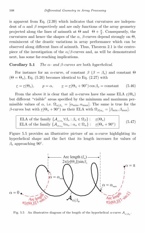
July 9, 2004 14:41 WSPC/Book Trim Size for 9in x 6in chap05
108 Differential Geometry in Array Processing
is apparent from Eq. (2.39) which indicates that curvatures are indepen-dent of α and β respectively and are only functions of the array geometryprojected along the lines of azimuth at Θ and Θ + π
2 . Consequently, thecurvatures and hence the shapes of the α, β-curves depend strongly on Θ,reminiscent of the drastic variations in array performance which can beobserved along different lines of azimuth. Thus, Theorem 2.1 is the centre-piece of the investigation of the α/β-curves and, as will be demonstratednext, has some far-reaching implications.
Corollary 5.1 The α- and β-curves are both hyperhelical.
For instance for an α-curve, of constant β (β = βo) and constant Θ(Θ = Θo), Eq. (5.20) becomes identical to Eq. (2.27) with
r = r(Θo), p = α, v = r(Θo + 90) cos βo = constant (5.46)
From the above it is clear that all α-curves have the same ELA r(Θo)but different “visible” areas specified by the minimum and maximum per-missible values of α, i.e. Ωα|βo = [αmin, αmax]. The same is true for theβ-curves but with r(Θo + 90) as their ELA with Ωβ|αo = [βmin, βmax].
ELA of the family Aα|βo
∀βo : βo ∈ Ωβ : r(Θo)ELA of the family A
β|αo∀αo : αo ∈ Ωα : r(Θo + 90)
(5.47)
Figure 5.5 provides an illustrative picture of an α-curve highlighting itshyperhelical shape and the fact that its length increases for values ofβo approaching 90.
Fig. 5.5 An illustrative diagram of the length of the hyperhelical α-curve Aα|βo
.

July 9, 2004 14:41 WSPC/Book Trim Size for 9in x 6in chap05
Non-Linear Arrays: (α, β)-Parametrization 109
Corollary 5.2 For a given frame rotation angle Θo, all members of thefamily of α- (or β-) curves of a planar array of N sensors are identi-cal (congruent) in shape apart from their length and position in complexN -dimensional space.
The above result means that the whole of the manifold surface may befully covered by the simple translation of either of the two individual curveswith displacement values given by v = r(Θo + 90) cos β0 for α-curves andv = r(Θo) cos α0 for β-curves. Note that α-curves are the same as β-curvesfor rotation Θo + 90.
Corollary 5.3 The α- and β-curves are identical to the θ-parametermanifold of a linear array of isotropic sensors with locations r(Θ) andr(Θ + π
2 ) respectively.
Figure 5.6 illustrates the α-β parametrization of the array manifold inthe special case of Θ = 0. Notice that for Θ = 0, cone-angles are mea-sured with respect to the x and y axes and consequently, according toCorollary 5.3, the α- and β-curves are identical to the θ-parameter man-ifolds of linear arrays with sensor locations r(0) = rx and r(π
2 ) = ry
respectively.Although the hyperhelical α (or β) family of curves shown above covers
the whole of the manifold surface and is sufficient to fully define the man-ifold shape, it is not unique. In fact, to understand the behavior of thearray for all possible directions of arrival, it is necessary to consider thehyperhelical coordinates corresponding to all values of Θ from 0 to π
2 .
Fig. 5.6 (θ, φ) and (α, β) parametrizations of the same manifold surface M with theframe rotation for the cone-angles Θo = 0.

July 9, 2004 14:41 WSPC/Book Trim Size for 9in x 6in chap05
110 Differential Geometry in Array Processing
Fig. 5.7 Families of α and β curves for a frame rotation Θo = 0. and for Θo < 90.
The above concept is more easily appreciated by observing Fig. 5.7which shows the effect of a non-zero value of Θ. It should be stressed that,despite the appearance of Fig. 5.7, the use of various values of Θ is notequivalent to a trivial rotation of the parameter curves, since their differ-ential geometry is a function of Θ (Corollary 5.3).
Figures 5.6 and 5.7 also reveal a clear relationship between the α (or β)curves and the hyperhelical φ-curves, which will be stated as the final twocorollaries:
Corollary 5.4 Each member of the α-curve family is identical in shapeto the combination of the φ-curves corresponding to θ = Θ and θ = Θ + π.Similarly each member of the β-curve family is identical to the combinationof the φ-curves at θ = Θ + π
2 and θ = Θ + 3π2 .
Corollary 5.5 The α-curve with β = 90 for a frame rotation Θo andthe composite φ curve A
φ|θo+ A
φ|(θo+π) are one and the same curve if andonly if θo = Θo.
Similarly the β-curve with α = 90 for a frame rotation Θo is one andthe same curve with the composite φ curve A
φ|θo+ A
φ|(θo+π) if and only ifθo = Θo + π
2 .
5.6 “Development” of α- and β-parameter Curves
The most significant implication of the property that the array manifoldM ∈CN of a planar array has a zero Gaussian curvature, is that M is a

July 9, 2004 14:41 WSPC/Book Trim Size for 9in x 6in chap05
Non-Linear Arrays: (α, β)-Parametrization 111
developable surface and hence can be isometrically mapped on to any othersurface of zero curvature, say a plane in R2. The result of such a mappingwould be a consistent two-dimensional representation (development) of themanifold in real space. A development may be readily evaluated by notingthat if A
α|βo,A
β|αo∈ CN are arbitrary α and β curves on the manifold
surface and A(d)α|βo
,A(d)β|αo
∈ R2 are their respective images on the develop-ment, then since an isometric mapping is by necessity both geodesic andconformal:
• Length of A(d)α|βo
∈ R2 = Length of Aα|βo
∈ CN ,• Principal curvature of A(d)
α|βo∈ R2 = Geodesic curvature of A
α|βo∈ CN ,
• (A(d)α|βo
, A(d)β|αo
) in R2 = (Aα|βo
, Aβ|αo
) in CN .
Fig. 5.8 (a) Square-grid array structure, ry⊥rx and ‖ry‖ = ‖rx‖ (balanced-symmetric).(b) Rectangular-grid array structure ry⊥rx and ry = 1.5 rx (unbalanced-symmetric).(c) and (d) Developments of the manifolds of arrays in Figs. (a) and (b) respectively whenthe manifolds are parametrized by cone-angles α and β with frame rotation Θ = 0.

July 9, 2004 14:41 WSPC/Book Trim Size for 9in x 6in chap05
112 Differential Geometry in Array Processing
Table 5.1 Cone-parametrizationmanifold parameters for 3D-gridand planar arrays.
Parameter 3D Planar
KG(Eq. (3.31))
1ρ2π2
0
κg,αcot β
ρπ0
κg,βcot α
ρπ0
The above features may be demonstrated by the following example.
Example 5.1 Consider the developments of the manifolds of two arrayconfigurations when parametrized with cone-angles α and β for Θ = 0
(recall that r(0) = rx and r(π/2) = ry). The array structures are indicatedin Figs. 5.8(a) and (b) with the respective developments in Figs. 5.8(c) and(d). Cone-angles α and β are considered in steps of 10 from 0 to 180.
Since both arrays are symmetric (i.e. rTx ry = 0), the α- and β-curves
are orthogonal and geodesic, as a result of which their images on the devel-opment are orthogonal straight lines (geodesics) and of length 2π
∥∥rx
∥∥sinβ
and 2π∥∥ry
∥∥sinα respectively. Note that the second array geometry is unbal-anced (
∥∥ry
∥∥ > ‖rx‖) and consequently the envelope of the development iselliptical rather than circular.
Finally, Table 5.1 summarizes the results associated with the Gaussianand geodesic curvatures indicating that for planar arrays both α and β
curves are geodesic curves. This indicates that the study of manifold geom-etry is considerably simplified as a result of (α, β) parametrization, onceagain confirming the advantages of cone-angles over azimuth and elevation.

July 7, 2004 14:4 WSPC/Book Trim Size for 9in x 6in chap06
Chapter 6
Array Ambiguities
In this chapter ambiguous sets of parameter values (e.g. directions) thatexist in any hyperhelical curve A embedded in an N dimensional complexspace, are modelled, identified and calculated. The curve A, which is definedas follows
A = a(p) ∈ CN , ∀p : p ∈ Ωp (6.1)
witha(p) = exp(−j(πr cos p + v)) (6.2)
could be the manifold of a linear array or a p-curve (with p = φ, α or β)lying on the manifold surface of a planar array (using the concept of theELA). In these cases the manifold vector a(p) represents the complexarray response to a unity power signal impinging on the array from direc-tion p and is a function of the locations r ∈ RN of the array elements,defined as
sensor locations : r r(Ψ0) = rx cos Ψ0 + ry sin Ψ0 (6.3)
The parameter Ψ0, shown in Fig. 6.1 and used in Eq. (6.3), is defined as
Ψ0
0 for any linear array on the x-axisθo for one φ-curve Aφ|θo
Θo for all α-curvesΘo + 90 for all β-curves
(6.4)
where θo is the constant azimuth (φ-curves) and Θo is the frame rotationangle (α-curves). Table 6.1 provides the main parameters of Eq. (6.2) forthe various hyperhelical array manifold curves.
113

July 7, 2004 14:4 WSPC/Book Trim Size for 9in x 6in chap06
114 Differential Geometry in Array Processing
Fig. 6.1 Equivalent linear array r(Ψ0).
Table 6.1 Array manifold vector parameters (Eq. (6.2)).
Parameter Linear Arrays Planar Arrays
p (generic) θ φ α β
Ωp ∈ R1 [0, π) [0, π/2) [0, π) [0, π)
r rx r(θo) r(Θo) r(Θo + 90)
h(p) = cos(p) cos(θ) cos(φ) cos(α) cos(β)
v 0 0 r(Θo + 90) cos(βo) r(Θo) cos(αo)
curve A Aφ|θo Aα|βo Aβ|αo
6.1 Classification of Ambiguities
The array manifold A of Eq. (6.1) is essentially a mapping from the param-eter space Ωp ∈ R1 to the complex N -dimensional space CN
p ∈ Ωparray geometry−→ a(p) ∈ C
N (6.5)
When finding the directions-of-arrival (DOA’s) of signals using array sensormeasurements, it is important to be certain that the problem has a uniquesolution. This is guaranteed if the above mapping is one-to-one.

July 7, 2004 14:4 WSPC/Book Trim Size for 9in x 6in chap06
Array Ambiguities 115
However, in this study we will consider the problem which arises whenthe mapping of Eq. (6.5) is not one-to-one. In this case the array cannot dis-tinguish between two (or more) different signal environments. For instancetwo different sets of signals impinging on the array can provide identicalresponses at the array output, i.e. the same measurements. In such a caseany estimation algorithm may be unable to distinguish the true parametervalues (e.g. directions) from the false ones. This is termed as the ambiguityproblem.
Definition 6.1 — Array Ambiguity: It is the inability of an array of agiven geometry to distinguish a set of parameter values
(p1, p2, . . . , pM ) with pi = pj ∈ Ωp for i = j (6.6)
from at least one of its subsets (or one subset from another).
Array ambiguities can be classified as “trivial” and “non-trivial.” Wewill start with trivial ambiguities.
Definition 6.2 — Trivial Ambiguities: An array ambiguity is said tobe classified as ‘trivial’ if there exist at least one pair p1, p2 ∈ Ωp withp1 = p2 such that
p1array geometry−→ a(p1) ∈ CN
p2array geometry−→ a(p2) ∈ CN
(6.7)
witha(p1) = ka(p2) (6.8)
and
k = scalar
In this case the two parameter values p1, p2 are indistinguishable by thearray.
Trivial ambiguities are the simplest type of ambiguity and can be easilyidentified/detected. For instance it is impossible to distinguish whether asignal is impinging on a linear array from direction-of-arrival p1 or from thedirection p2 = 360 − p1, i.e. the mirror image of p1 with respect to 180.In this case
a(p1) = a(p2) (6.9)

July 7, 2004 14:4 WSPC/Book Trim Size for 9in x 6in chap06
116 Differential Geometry in Array Processing
and for this reason, in order to avoid this ambiguity problem, the parameterspace in the case of linear arrays is confined to Ωp = [0, 180).
However, Eq. (6.9) is a special case of Eq. (6.8) for k = 1. Eq. (6.8) indi-cates that there exists at least one manifold vector a(p2) which is colinearto another manifold vector a(p1). Then the two waves with bearings p1, p2
are indistinguishable by the array even if p1, p2 ∈ Ωp = [0, 180).Non-trivial ambiguities are a more complicated type of ambiguity arising
when a manifold vector can be written as a linear combination of two ormore different manifold vectors.
Definition 6.3 — Non-Trivial Ambiguities: An array ambiguity issaid to be classified as “non-trivial” if there exist at least a set of valuesp1, p2, . . . , pM ∈ Ωp with M > 2 and pi = pj for i = j such that
pi ∈ Ωparray geometry−→ a(pi) ∈ CN ; ∀i = 1, 2, . . . , M (6.10)
witha(pM ) = c1a(p1) + c2a(p2) + · · · + cM−1a(pM−1) (6.11)
Then this set (p1, p2, . . . , pM ) and all its subsets of M − 1 elements areindistinguishable by the array.
In such a case the array will have identical responses for the sets ofbearings (p1, p2, . . ., pM−1), (p2, p3, . . ., pM ), (p1, p3, p4, . . ., pM ), etc.
Fig. 6.2 illustrates a non-trivial ambiguous situation where the manifoldvector a(p3) belongs to the subspace L [A] where A = [a(p1),a(p2)].
This type of ambiguity is much more difficult to identify since,unlike a trivial ambiguity, it cannot be detected by a simple searchof the manifold. For example consider the non-uniform linear arrayof four sensors with sensor locations (measured in half wavelengths)given by
r = [−2, −1, 1, 2]T (6.12)
One non-trivial ambiguity of this array is related to the set of directions
0, 60, 90, 120
as the array is unable to distinguish between the following signalenvironments:
(0, 60, 90), (0, 60, 120), (60, 90, 120), (0, 60, 90, 120)
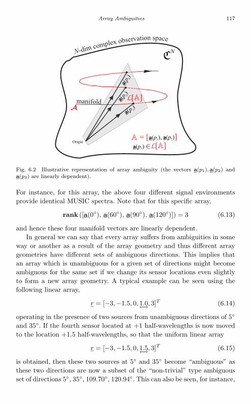
July 7, 2004 14:4 WSPC/Book Trim Size for 9in x 6in chap06
Array Ambiguities 117
Fig. 6.2 Illustrative representation of array ambiguity (the vectors a(p1),a(p2) anda(p3) are linearly dependent).
For instance, for this array, the above four different signal environmentsprovide identical MUSIC spectra. Note that for this specific array,
rank ([a(0), a(60), a(90), a(120)]) = 3 (6.13)
and hence these four manifold vectors are linearly dependent.In general we can say that every array suffers from ambiguities in some
way or another as a result of the array geometry and thus different arraygeometries have different sets of ambiguous directions. This implies thatan array which is unambiguous for a given set of directions might becomeambiguous for the same set if we change its sensor locations even slightlyto form a new array geometry. A typical example can be seen using thefollowing linear array,
r = [−3,−1.5, 0, 1.0←→, 3]T (6.14)
operating in the presence of two sources from unambiguous directions of 5
and 35. If the fourth sensor located at +1 half-wavelengths is now movedto the location +1.5 half-wavelengths, so that the uniform linear array
r = [−3,−1.5, 0, 1.5←→, 3]T (6.15)
is obtained, then these two sources at 5 and 35 become “ambiguous” asthese two directions are now a subset of the “non-trivial” type ambiguousset of directions 5, 35, 109.70, 120.94. This can also be seen, for instance,

July 7, 2004 14:4 WSPC/Book Trim Size for 9in x 6in chap06
118 Differential Geometry in Array Processing
Fig. 6.3 MUSIC spectrum in an “ambiguous” situation.
from Fig. 6.3 where in the MUSIC spectrum, four nulls appear at directions5, 35, 109.70, 120.94 rather than two at 5 and 35.
Note that in this study the array centroid will be taken as the referencepoint, implying that sum(r)= rT 1N = 0. However, it can be proved thatthe ambiguities are independent of the choice of the array reference point.
6.2 The Concept of an Ambiguous Generator Set
Before continuing it is necessary to present the following definitions whichwill be extensively used.
Definition 6.4 — Ambiguous Set and Rank of Ambiguity
(1) Ambiguous Set:An ordered set of arc lengths s = [s1, s2, . . . , sc]T , is said to be anambiguous set of arc lengths
if c ≤ N and the matrix A(s) ∈ CN×c with columns the manifold vec-tors a(s1), a(s2), . . . , a(sc) has rank less than c, i.e. rank(A(s)) < c
or
if c > N and all subsets si of s which contain exactly N elementsare themselves ambiguous sets of arc lengths,
i.e. rank(A(si)) < N, ∀i (6.16)

July 7, 2004 14:4 WSPC/Book Trim Size for 9in x 6in chap06
Array Ambiguities 119
(2) Rank of Ambiguity:For an ambiguous set of arc lengths s = [s1, s2, . . . , sc]T its rank ofambiguity is defined as the integer ρa
where ρa =
rank(A(s)) if c N
min∀i
rank (A(si)) if c > N (6.17)
with si ∈ RN ,∀i.
Note that the previously introduced definitions can be directly appliedto sets of directional parameters by simply substituting (using Eq. (2.28))the arc length s with p.
The following theorem, which is a very important result, essentiallystates that if all the elements of an ambiguous set of arc lengths are rotatedon the array manifold by the same value, then the resulting set is also anambiguous set of arc lengths.
Theorem 6.1 — Arc length Rotation: For a linear array of N sen-sors, if
s = [s1, s2, . . . , sc]T (6.18)
is an ambiguous set of arc lengths with rank of ambiguity ρa, then any set
s = [s1 + ∆s, s2 + ∆s, . . . , sc + ∆s]T
= s + ∆s.1c, (6.19)
with s1 +∆s ≥ 0 and sc +∆s ≤ lm, is also an ambiguous set of arc lengthswith the same rank of ambiguity ρa.
The proof of this theorem can be found in Appendix 6.7.1 while itsessential features are illustrated in the following example.
Example 6.1 Consider a linear array having sensor locations given, inhalf-wavelengths, by the following vector:
r = [−3,−1,−0.5, 2, 2.5]T
and having a manifold length lm = 2π‖r‖ = 28.4483. It can easily be seenthat the set
p = [0, 53.13, 78.46, 101.54, 126.87]T

July 7, 2004 14:4 WSPC/Book Trim Size for 9in x 6in chap06
120 Differential Geometry in Array Processing
is an ambiguous set of directions. Using Eq. (2.28) the correspondingambiguous set of arc lengths is computed to be
s = [0, 5.6897, 11.3793, 17.0690, 22.7857]T
If this set s is rotated by ∆s = 2, then a new set of arc lengths
s = [2, 7.6897, 13.3793, 19.0690, 24.7857]T
is obtained, which corresponds to the set of directions
p = [30.75, 62.65, 86.59, 109.91, 137.78]T
which is also an ambiguous set. This is also true for any ∆s so long as thelast element of s is smaller than, or equal to, the manifold length lm. Notethat the rotation should be carried out in the “arc length” domain and notin the “directions-of-arrival” domain (parameter p domain). For instance,if the directions of the original sources are rotated by ∆p = 20 so that thenew set of directions
p + ∆p15 = [20, 73.13, 98.46, 121.54, 146.87]T
is obtained, then this set is not ambiguous.Furthermore any subset of 4 elements of p or p are also ambiguous sets of
directions. If the array operates in the presence of 4 sources with directionsany subset of 4 elements of p will give the same MUSIC spectrum.
It becomes clear that if one ambiguous set is identified, then by simplerotation in arc lengths, an infinite number of ambiguous sets can be gen-erated and therefore two different ambiguous sets may in fact be just arotation of each other. It is an impossible task to try to identify all theambiguous sets and, since all these sets can be generated from a single set,the idea of the ambiguous generator set arises, defined as follows:
Definition 6.5 — Ambiguous Generator Set: An ordered set s =[s1, s2, . . . , sc]T of c arc lengths, where 2 ≤ c ≤ N , is said to be an ambigu-ous generator set (AGS) of arc lengths if and only if:
(a) s1 = 0 and sj = 0 with 2 ≤ j ≤ c. That is, all the elements of the setbut the first element are non-zero.
(b) the rank of the N × c matrix A(s) with columns the manifold vectorsassociated with the elements of the set is less than c, i.e.
rank(A(s)) ρa < c (6.20)

July 7, 2004 14:4 WSPC/Book Trim Size for 9in x 6in chap06
Array Ambiguities 121
(c) for any subset si of m elements of s (including s1 = 0) with ρa ≤ m < c,the rank of A(si) is equal to ρa
According to the previous definition, a set of arc lengths s =[s1, s2, s3, s4]T with s1 = 0, s2, s3, s4 = 0 and a(s3) = c1a(s1) + c2a(s2)is not an ambiguous generator set. This is because
rank([a(s1),a(s2),a(s3),a(s4)]) = 3 (6.21)
but
rank([a(s1),a(s2),a(s3)]) = 2 (6.22)
(i.e. third condition is not satisfied). On the other hand, the subset[s1, s2, s3]T is an ambiguous generator set since it satisfies all the threeconditions of Definition 6.5.
The next section is concerned with the identification of ambiguous gen-erator sets (AGS) existing in the manifold of a linear array of arbitrarygeometry.
6.3 Partitioning the Array Manifold Curve into Segmentsof Equal Length
In this section a framework is proposed for the calculation of a type ofambiguous generator sets of directions existing in linear arrays of any geom-etry, as well as their associated rank of ambiguity. The framework is basedon the uniform partitioning of the array manifold hyperhelix, obtained bydividing the manifold length lm by the difference between any two arraysensor locations. Note that from now on the vector r with elements thesensor locations (in half-wavelengths) will be assumed to be ordered in thesense that ri < rj ⇔ i < j. Furthermore, the absolute difference betweenthe i-th and j-th sensor locations, measured in half-wavelengths, will bedenoted by ∆rij > 0 and hence the aperture of the array will be ∆r1,N .Note that the term “intersensor spacing” will refer to the spacing betweenany two sensors, not necessarily adjacent.
Thus one type of array ambiguity can be identified by dividing a hyper-helical manifold curve into equal segments, according to the followingtheorem.
Theorem 6.2 — Uniform-Partition Type Ambiguities: Consider alinear array (or an ELA) of N sensors, with locations r = [r1, r2, . . . , rN ]T
and let lm denote the length of its hyperhelical manifold curve embedded in

July 7, 2004 14:4 WSPC/Book Trim Size for 9in x 6in chap06
122 Differential Geometry in Array Processing
CN . By uniformly partitioning this hyperhelix into segments of arc lengthlm
∆rijwhere ∆rij = |ri − rj | with i = j, a set of c points on the manifold
curve can be identified, forming the vector
s∆rij=[0,
lm∆rij
, 2lm
∆rij, . . . , (c − 1)
lm∆rij
]T(6.23)
where
c =
1 + fix(∆rij) if ∆rij /∈ N+
∆rij if ∆rij ∈ N+
and fix (•) denotes the integer part of a number
(a) If c ≥ N then any subset of s∆rij∀i, j with N elements is an ambiguous
set.(b) if c < N then s∆rij
∀i, j might be an ambiguous set.
Proof. The proof of this theorem is as follows. Consider a linear array ofN sensors with locations r. If the difference between the ith and jth sensorlocations, i.e. ∆rij = |ri − rj |, satisfies c ≥ N , then we have to prove thatany subset of N elements of the set of arc lengths s∆rij
of Eq. (6.23) is anambiguous set.
Using the manifold vector expressed in terms of arc length, i.e.
a(s) = exp(j(rs − πr + v)) (6.24)
in conjunction with
lm = 2π ‖r‖ and r =r
‖r‖ (6.25)
the matrix A(s∆ri,j) ∈ CN×c with columns the associated manifold vectors
can be written as follows:
A(s∆rij) =
[exp (j (−πr + v)) , exp
(j(
2π∆rij
r − πr + v))
, . . . ,
exp(j((c − 1) 2π
∆rijr − πr + v
))](6.26)
Since c N the number of columns of A(s∆rij) is equal to, or greater than,
N. Hence, by taking a submatrix of AN of A with exactly N elements, e.g.the N first columns of A, we have the following square submatrix denoted

July 7, 2004 14:4 WSPC/Book Trim Size for 9in x 6in chap06
Array Ambiguities 123
by AN
AN =[exp (j (−πr + v)) , exp
(j(
2π∆rij
r − πr + v))
, . . . ,
exp(j((c − 1) 2π
∆rijr − πr + v
))]= diag(exp (j (−πr + v)) AN (6.27)
where
AN =[1N , exp
(j2π
1∆rij
r
), . . . , exp
(j(2π(N − 1)
1∆rij
r
)](6.28)
Consider now the ith and jth rows of AN with i > j. By using theproperty that
exp(
−j2πk∆rij
∆rij
)= 1, ∀k ∈ N+ (6.29)
the ith row of AN can be written as follows
rowTi (AN ) = IN · rowT
i (AN )
=
1 0 0 . . . 00 exp
(−j2π∆rij
∆rij
)0 . . . 0
0 0 exp(−j2π2∆rij
∆rij
). . . 0
0 0 0 . . . 00 0 0 . . . exp
(−j2π(N − 1)∆rij
∆rij
)
.
[1N , exp
(j2πri
1∆rij
), . . . , exp
(j2πri (N − 1) 1
∆rij
)]T
=[1N , exp
(j2π
ri−∆rij
∆rij
), . . . , exp
(j2π(N − 1) ri−∆rij
∆rij
)]T
=[1N , exp
(j2π
rj
∆rij
), . . . , exp
(j2π(N − 1) rj
∆rij
)]T
= rowTj (AN )
i.e.
rowi(AN ) = rowj(AN )
=⇒ det(AN
)= 0 =⇒ det (AN ) = 0 (6.30)

July 7, 2004 14:4 WSPC/Book Trim Size for 9in x 6in chap06
124 Differential Geometry in Array Processing
It is easy to see that the fact that AN was chosen to consist of the first N
columns of A, and not any N columns, is not restrictive in the least sincethe ith and the jth rows of any N × N submatrix of A will be equal. Sinceall submatrices AN of A are singular, it results that A is rank deficient andtherefore, any subset of s∆ri,j
with exactly N elements is an ambiguous set.
Note that
c =
1 + fix(∆rij) if ∆rij /∈ N+
∆rij if ∆rij ∈ N+=⇒ c < 1 + ∆rij =⇒ (c − 1)
lm∆rij
< lm
(6.31)
indicating that the last element of the vector s∆rijof Eq. (6.23), is smaller
that the manifold length lm. The vector s∆rijwith elements c ∈ N+ man-
ifold points will be known as the “uniform basic set” (UBS) of arc lengthsassociated with the intersensor spacing ∆rij as it is constructed by uni-formly partitioning the manifold length by the spacing ∆rij between theith and jth sensors.
According to Theorem 6.2, all subsets of N elements from a set s∆rij,
of the form of Eq. (6.23) are ambiguous sets but not necessarily ambiguousgenerator sets. In order for such a subset to be an ambiguous generatorset it must have its first element equal to zero and also satisfy the thirdcondition of the ambiguous generator set in Definition 6.5.
From the investigation of the precise cause of the ambiguous natureof the set of arc lengths s∆rij
constructed by uniformly partitioning themanifold length by the spacing ∆rij , it is clear that the most commonAGSs are of rank N −1. However, AGSs of rank less than (N −1) can existif more pairs of rows of the determinant matrix AN
(s∆rij
)are identical.
This is possible if the array geometrical structure satisfies certain specialconditions and for this reason we need the following definition.
Definition 6.6 — A “Distinct” Set of Intersensor Spacings: In alinear array of N sensors, a set of k intersensor spacings is said to be a“distinct” set if no intersensor spacing is a combination of the other spacingsin the set. There are N(N − 1)/2 intersensor spacings but at most (N − 1)elements in a distinct set of intersensor spacings (i.e. k N − 1)).
For instance, if ∆rij and ∆rjk are members of a distinct set with i =j = k then ∆rik is not a member.

July 7, 2004 14:4 WSPC/Book Trim Size for 9in x 6in chap06
Array Ambiguities 125
Based on the above definition, the following theorem states that if thereare distinct sets of intersensor spacings then AGSs of rank less than (N −1)may be found.
Theorem 6.3 — Number of AGSs of a given rank: Consider an N -sensor linear array. If k∆rij
denotes the elements of a distrinct set of inter-sensor spacings which are integer multiples of the smallest (∆rij) amongstthem, and
∆rij (N − k∆rij
)(6.32)
then the Uniform Basic Set s∆rijof c elements is an ambiguous set from
whichmin(N−1,c−1)∑
=N−k∆rij
(c − 1
)(6.33)
ambiguous generator sets of rank-(N − k∆rij
)can be constructed.
The implication of the above theorem to the number of ambiguous gen-erator sets of a linear array is twofold. Firstly, it reveals the existence ofadditional ambiguous generator sets corresponding to intersensor spacingswhich are less than (N − 1), provided that they occur in integer multiples ofeach other, which includes the special case of repeated occurrences. In par-ticular, if a spacing, say ∆rij , occurs k∆rij
times then the size of this spacingneed only be
(N − k∆rij
)to give rise to ambiguous generator sets. Secondly,
the larger the k∆rij is, the more rank-(N − k∆rij
)ambiguous generator sets
can be constructed. This point can be illustrated from the intersensor spac-ings ∆r13 = ∆r24 = 4.1 of the linear array r = [−3 ,−2.2 , 1.1 , 1.9 , 2.2 ]T
where k∆r13 = 2 and ∆r13 (N − k∆r13) = 3. Thus from s∆r1,3, five
rank-3 ambiguous generator sets can be constructed (instead of a singlerank-4 set).
From the array’s geometrical perspective, the following statement withrespect to rank-
(N − k∆rij
)ambiguity can be made:
Corollary 6.1 If k intersensor spacings of an N -sensor linear arrayare integer multiples of the smallest among them, with the latter being atleast (N − k) half-wavelengths, then the array suffers from rank-(N − k)ambiguity.
In summary the reason for the existence of these lower than N − 1 rankambiguities can easily be deduced from the definition of the ambiguous

July 7, 2004 14:4 WSPC/Book Trim Size for 9in x 6in chap06
126 Differential Geometry in Array Processing
generator set and especially its third condition (see Definition 6.5). Moreanalytically, it can be easily derived from the proof of Theorem 2.1, thatif two or more intersensor spacings of a linear array (or ELA) are integermultiples of each other (which is the case for either of the above conditions)and if s is an ambiguous generator set associated with the smallest of theseintersensor spacings, then the manifold matrix A(s) may have more thantwo identical rows. This implies that its rank will be smaller than N − 1.
As a direct result of Theorem 6.3 and of the previous corollary it canbe said that the uniform linear array (or ELA) with intersensor spacing∆r1,2 1 suffers from trivial ambiguities. Indeed, the intersensor spacing∆r = ∆r1,2 occurs N−1 times. That is ∆r1,2 = ∆r2,3 = · · · = ∆rN−1,N , i.e.
k∆rij= N − 1 =⇒ ρa = N − N + 1 = 1 (6.34)
This well known result is rediscovered by observing that in such a case theset s∆ri,j
will contain at least two elements and the matrix A will be rankdeficient since all its rows will be equal.
By setting the value of ∆rij = |ri−rj | in the above equation to be equalto the biggest possible difference between two array sensor locations, whichis obviously the aperture la = ∆r1,N , and by combining the above with theTheorem 6.2(a), the following sufficient condition can be obtained.
Corollary 6.2 A SUFFICIENT condition for the presence of ambiguitiesin ALL linear arrays of N sensors, is
la > N − 1 where la = max∀i,j
∆rij = ∆r1,N (6.35)
It should be clear however, that the above provides a sufficient butby no means necessary condition for the presence of ambiguities. Thismeans that a linear array (or ELA) can possibly suffer from ambiguitieseven if la ≤ N − 1 half wavelengths. Only for the specific case of uniformlinear (or ELA) arrays, has it been proven that no ambiguities exist ifla ≤ N − 1 or, equivalently, if the intersensor spacing is not greater thanhalf a wavelength.
Theorem 6.2 has an implication that needs to be stressed. It is wellknown that an increase in the aperture results in better resolution capabili-ties. However, from the point of view of ambiguities, increasing the aperturemay not be a very good idea. By increasing the aperture, the number ofelements in the set of Eq. (6.23) increases, and once this number becomesgreater than N − 1, the set becomes ambiguous. Furthermore, increasingall the intersensor spacings may be considered an even more serious issue

July 7, 2004 14:4 WSPC/Book Trim Size for 9in x 6in chap06
Array Ambiguities 127
since an array with sensor locations given by r = br, with b > 1, mighthave many intersensor spacings ∆rij which result in ambiguous sets of theform given in Eq. (6.23).
Example 6.2 Consider an array with sensor locations given by r =[−2.1,−0.9, 0.9, 2.1]T . The manifold length lm of this array is calculatedto be 20.3016. Furthermore, the only absolute difference between sensorlocations satisfying c N is the aperture ∆r1,4 = 4.2. This provides thefollowing uniform basic set of arc lengths:
s∆r1,4= [0, 4.8337, 9.6674, 14.5011, 19.3348]T
According to Theorem 6.2, any subset of 4 elements (N = 4) from the aboveset will be an ambiguous set and the matrix A with columns the manifoldvectors corresponding to such a subset will be singular. Furthermore, it canbe shown that no matrix A corresponding to any three elements of s∆r1,4
is rank deficient. This means that four different ambiguous generator setscan be identified from s∆r1,4
which are all the subsets of s∆r1,4with their
first element zero and three non-zero elements of s∆r1,4. As expected from
Theorem 6.2, the set s∆r1,4is ambiguous since c ≥ N . However, ambiguous
sets might also be defined from Theorem 6.2 when c < N . To see this,consider the uniform basic set for the difference ∆r1,3 = ∆r2,4 = 3 (i.e.k∆r1,3 = 2), which is c = 3 < N = 4
s∆r1,3= s∆r2,4
= [0, 6.7672, 13.5344]T
=⇒ θ∆r1,3= θ∆r2,4
= [0, 70.53, 109.47]T
If the matrix A with columns the corresponding manifold vectors isobtained, then rank(A) = 2 and hence the above set is an ambiguousset with rank of ambiguity equal to 2. It should also be noted that not allthe uniform basic sets s∆ri,j
resulting from a difference ∆rij between twosensor locations are ambiguous if c < N . To see this, consider the differ-ences ∆r1,2 = ∆r3,4 = 1.2 (or ∆r2,3 = 1.8) of the previous array whichresults in the set s∆r1,2
= [0, 16.9180]T (or s∆r2,3= [0, 11.2787]T ) (i.e.
c = 2 < N = 4) which is unambiguous.
So far it has been shown that Theorem 6.2 can be used in order toidentify ambiguous sets inherent in linear arrays of any geometry. Whenthis theorem is focused on specific array geometries it can produce somemore useful results as the following corollaries indicate.

July 7, 2004 14:4 WSPC/Book Trim Size for 9in x 6in chap06
128 Differential Geometry in Array Processing
Corollary 6.3 All the ambiguous sets that exist in a two-element arraycan be calculated from Eq. (6.23).
Proof. The proof is as follows. Consider the two-element array r =[−r1, r1]. Let s = [s1, s2]T with s1 = 0 being an ambiguous set of arclengths. The matrix A with columns the manifold vectors correspondingto s is
A = [a(0),a(s2)]
=
exp(jπr1) exp(
jπr1
(1 − s2
π ‖r‖))
exp(−jπr1) exp(
−jπr1
(1 − s2
π ‖r‖))
(6.36)
Since it is assumed that s is an ambiguous set, it results that A is singularand therefore
det(A) = exp(jπr1). exp(
−jπr1
(1 − s2
π ‖r‖))
− exp(−jπr1). exp(
jπr1
(1 − s2
π‖r‖))
= 0
=⇒ exp(
jπr1s2
π‖r‖)
− exp(
−jπr1s2
π‖r‖)
= 0
=⇒ sin(
r1s2
‖r‖)
= 0
=⇒ r1s2
‖r‖ = kπ with k = 1, 2, 3, . . . (since s2r1 = 0)
=⇒ s2 = kπ‖r‖r1
= k2π‖r‖2r1
= k2π‖r‖∆r1,2
= klm
∆r1,2That is
s1 = 0 and s2 = klm
∆r1,2(6.37)
withk = 1, 2, 3, . . .
Therefore the only ambiguous set of arc lengths that can possibly exist fora two-element array are of the form of Eq. (6.23). As a result, a necessaryand sufficient condition for the presence of ambiguities in a two elementlinear array is
lm∆r12
< lm =⇒ ∆r12 > 1 (6.38)

July 7, 2004 14:4 WSPC/Book Trim Size for 9in x 6in chap06
Array Ambiguities 129
Corollary 6.4 The set of arc lengths s = [0, π√
2, 2π√
2, . . . , (c−1)π√
2]T
is an ambiguous Uniform Basic Set for all three-element symmetric lineararrays, as long as ∆r1,3 > 2.
Proof. For all three-element symmetric linear arrays with sensor pos-itions given by r = [−r1, 0, r1]T , the manifold length is equal to
lm = 2π‖r‖ = 2π√
(−r1)2 + (r1)2 = 2πr1√
2 (6.39)
The Uniform Basic Set s∆r1,3associated with the difference between the
first and the third sensors is
s =[0, lm
∆r1,3, 2 lm
∆r1,3, . . . , (c − 1) lm
∆r1,3
]T
=[0, 2πr1
√2
2r1, 2 2πr1
√2
2r1, . . . , (c − 1) 2πr1
√2
2r1
]T
=[0, π
√2, 2π
√2, . . . , (c − 1)π
√2]T
(6.40)
Corollary 6.5 Let two arrays of N sensors have a common difference∆r between two sensor locations. The Uniform Basic Set of arc lengthsassociated with the common ∆r is different for these two arrays but thecorresponding ambiguous sets of DOA’s are the same.
Proof. Consider two different linear arrays (or ELAs) each having N
sensors with sensor locations r1 and r2. Let there be a common dif-ference ∆r between two sensor locations, which, for both arrays, satisfythe conditions of Theorem 6.2. In this case, the two Uniform Basic Setswill be:
First array:
s1 =[0,
2π‖r1‖∆r , 2 2π‖r1‖
∆r , . . . , (c − 1) 2π‖r1‖∆r
]T
(6.41)
Second array:
s2 =[0,
2π‖r2‖∆r , 2 2π‖r2‖
∆r , . . . , (c − 1) 2π‖r2‖∆r
]T
(6.42)
with c N , which implies that the above two sets are ambiguous. UsingEq. (2.28) the corresponding set of DOA’s for the first array is
θ1 =[0, arccos
(1 −
2π‖r1‖∆r
π‖r1‖
), . . . , (c − 1) arccos
(1 −
2π‖r1‖∆r
π‖r1‖
)]T
=[0, arccos
(1 − 2
∆r
), . . . , (c − 1) arccos
(1 − 2
∆r
)]T(6.43)

July 7, 2004 14:4 WSPC/Book Trim Size for 9in x 6in chap06
130 Differential Geometry in Array Processing
whereas, for the second array
θ2 =[0, arccos
(1 −
2π‖r2‖∆r
π‖r2‖
), . . . , (c − 1) arccos
(1 −
2π‖r2‖∆r
π‖r2‖
)]T
=[0, arccos
(1 − 2
∆r
), . . . , (c − 1) arccos
(1 − 2
∆r
)]T(6.44)
The two sets are obviously identical.
6.3.1 Calculation of Ambiguous Generator Sets of Linear(or ELA) Array Geometries
For a given linear array (or ELA) with sensor locations given by r andbased on Theorem 6.2, the following technique (presented in a step by stepform) provides a table with rows all the ambiguous generator sets, and theirassociated rank of ambiguity:
(1) For a given array with sensor locations r, calculate the manifold lengthlm = 2π‖r‖.
(2) Calculate the intersensor spacings by taking the Kronecker differencebetween the vector r (with elements the sensor locations) and itself,i.e. r r, which results in a (N2 × 1)-dimensional real vector. Create anew vector ∆r by keeping all the positive elements of r r. Due to theproperties of the Kronecker difference N elements of r r will be equalto zero and half of the remaining elements will be negative. Therefore,∆r ∈ Rd×1, where d = N
2 (N − 1).(3) Redefine ∆r by eliminating all elements which are smaller than one, i.e.
d ≤ N2 (N − 1). Note that the elements of ∆r which are smaller than
one provide
c = 1 + fix(∆rij) = 1 + 0 = 1 (6.45)
and therefore cannot possibly give rise to ambiguous generator sets.(4) For each element of ∆r, i.e. for each difference ∆rij = |ri − rj | > 1
between two sensor locations, construct the “Uniform Basic Set” vectors∆rij
using Eq. (6.23). Note that there are d different vectors s∆rijand
that each s∆ri,jcorresponds to a different uniform partition of the array
manifold.(5) Identify all the vectors s∆rij
, with c < N and then eliminate those forwhich:
rank(A(s∆rij)) = c < N

July 7, 2004 14:4 WSPC/Book Trim Size for 9in x 6in chap06
Array Ambiguities 131
Form the “Table of Ambiguous Uniform Basic Sets” with rows all theremaining vectors s∆rij
. All these vectors are ambiguous sets and pro-duce ambiguous generator sets. It is obvious that the set with the max-imum number of elements is the set s∆r1,N
.(6) For each s∆rij
(i.e. for each row of the “Table of Uniform Basic Sets”)construct the AGSs (and associated rank of ambiguity), according tothe following rules:
Rule (a) If the non-zero elements of s∆rijcannot be found in any
other “Uniform Basic Set” vector, then(c − 1N − 1
)ambiguous generator sets
can be produced by this s∆rij. These ambiguous genera-
tor sets are all the possible subsets of N elements of s∆ri,j
with their first element zero and N − 1 non-zero elementsof s∆rij
.
All ambiguous generator sets constructedin this way have rank of ambiguity
ρa = N − 1
Note that such rows must definitely have c ≥ N (seeTheorem 6.2), otherwise they would have been eliminatedin Step 5.
Rule (b) If the non-zero elements of s∆ri,jcan be found in other rows,
then ambiguous generator sets with rank of ambigu-ity less than N − 1 might be obtained. This meansthat all subsets of s∆ri,j
with their first element 0 and withlengths 2, 3, . . . ,min(N −1, c−1) must be considered. Thesesubsets are classified as ambiguous generator sets if the threeconditions of the ambiguous generator set definition (seeDefinition 6.5) are satisfied. Furthermore, for each ambigu-ous generator set s, rank of ambiguity ρa = rank(A(s∆ri,j
))is estimated. Note that this step clarifies why in Step 5 itis incorrect to eliminate two s∆ri,j
vectors which are thesame, although they will result in the same ambiguous gen-erator sets.
(7) Create the Ambiguous Generator Table of the array whose rows areall the different ambiguous generator sets (and their associated rank

July 7, 2004 14:4 WSPC/Book Trim Size for 9in x 6in chap06
132 Differential Geometry in Array Processing
of ambiguity) found in Step 6. Also, eliminate rows of s∆ri,jwhich are
duplicates.
6.4 Representative Examples
An indicative example of the above technique is presented below.
Example 6.3 The steps of the previously described technique for anarray of N = 5 sensors with sensor positions r = [−3,−2.2, 1.1, 1.9, 2.2]T
are as follows:
(1) The manifold length of this array is computed to be lm = 30.4589.(2) The Kronecker difference between r and itself, reshaped in the form of
an N × N matrix, is0, −0.8, −4.1, −4.9, −5.2,
0.8, 0, −3.3 −4.1 −4.4,
4.1, 3.3, 0, −0.8, −1.14.9, 4.1, 0.8, 0, −0.35.2, 4.4, 1.1, 0.3, 0
(3) Eliminating those entries of r r which are smaller than unity results in
∆r =
∆r1,3 = 4.1∆r1,4 = 4.9∆r1,5 = 5.2∆r2,3 = 3.3∆r2,4 = 4.1∆r2,5 = 4.4∆r3,5 = 1.1
(6.46)
(4) The seven Uniform Basic Sets (vectors) s∆ri,jare given in Table 6.2.
(5) The Uniform Basic Sets s∆rijwhich have less than N = 5 elements (i.e.
c < N) are examined. These are the sets s∆r2,3and s∆r3,5
.
• The number of elements in s∆r2,3is 4 < N = 5 and, furthermore,
rank (A(s∆r2,3)) = 4 = c and hence this row is eliminated.
• Also, s∆r3,5is eliminated since c = 2 < N = 5 and
rank(A(s∆r2,3)) = 2 = c. (6.47)
Thus the remaining sets are s∆r1,3, s∆r1,4
, s∆r1,5, s∆r2,4
and s∆r2,5.
(6) In this step, the AGSs arising from the remaining Uniform Basic Setsare calculated based on the rules (6a) and (6b).

July 7, 2004 14:4 WSPC/Book Trim Size for 9in x 6in chap06
Array Ambiguities 133
Table 6.2 Uniform Basic Sets of ∆rij > 1.
s1 s2 s3 s4 s5 s6
sT∆r1,3
0 7.4290 14.8580 22.2870 29.7160 —
sT∆r1,4
0 6.2161 12.4322 18.6483 24.8644 —
sT∆r1,5
0 5.8575 11.7150 17.5725 23.4300 29.2875
sT∆r2,3
0 9.2300 18.4600 27.6900 — —
sT∆r2,4
0 7.4290 14.8580 22.2870 29.7160 —
sT∆r2,5
0 6.9225 13.8450 20.7675 27.6900 —
sT∆r3,5
0 27.6900 — — — —
The non-zero elements of s∆r1,4, s∆r1,5
and s∆r2,5cannot be found
in any other s∆ri,jand hence should be investigated based on rule 6a.
The non-zero elements of s∆r1,3can also be found in s∆r2,4
and vice-versa and hence should be investigated based on rule 6b. The above aresummarized in Table 6.3.
Table 6.3 Rules for examining the UBSs of Table 6.2.
c ρa rule
sT∆r1,3
5 3 (6b)sT∆r1,4
5 4 (6a)
sT∆r1,5
6 4 (6a)
sT∆r2,3
4 4 removed
sT∆r2,4
5 3 (6b)
sT∆r2,5
5 4 (6a)sT∆r3,5
2 2 removed
Based on Rule (6a)
• s∆r1,4: Since the number of the elements of s∆r1,4
is 5 (c = 5),we have
(c−1N−1
)=(44
)= 1 which implies that only one ambiguous
generator set (which is the same as the Uniform Basic Set s∆r1,4)
can be identified, with ρa = 4.• s∆r1,5
: This time c = 6 and therefore(
c−1N−1
)=(54
)= 5 ambiguous
generator sets can be found by taking all the subsets of N elementsof s∆r1,5
(with one zero and N − 1 non-zero elements). Each of thesesets has ρa = 4.

July 7, 2004 14:4 WSPC/Book Trim Size for 9in x 6in chap06
134 Differential Geometry in Array Processing
• s∆r2,5: Finally, s∆r2,5
has c = 5 and it generates(
c−1N−1
)=(44
)= 1
ambiguous generator set. This AGS is the same as set s∆r2,5and has
ρa = 4.
Based on Rule (6b)
• s∆r1,3: The non-zero elements of s∆r1,3
can also be found in s∆r2,4
and hence s∆r1,3is investigated based on rule 6b. The ambiguous
generator set definition is initially checked for the set s∆r1,3. This
set is certainly ambiguous and the matrix with columns the corre-sponding manifold vectors has
rank(A(s∆r1,3
))
= 3 < c = 5 (6.48)
However, any one of the four subsets s with four elements of s∆r1,3
involving one zero and three non-zero elements, is also an ambiguousset. The matrix with columns the corresponding manifold vectors hasrank(A(s)) = 3 < c = 5. Therefore, the set s∆r1,3
satisfies the thirdcondition of the definition of the ambiguous generator set. Similarly,the four subsets s are ambiguous generator sets since all their sub-sets with three elements are unambiguous. Hence, the following fiveambiguous generator sets can be defined from s∆r1,3
, all of whichhave ρa = 3. Indeed
min(N−1,c−1)∑=N−k∆rij
(c − 1
)=
min(4,4)∑=5−2
(5 − 1
)
=4∑
=3
(4
)=(
43
)+(
44
)= 5 (6.49)
• s∆r2,4: Since s∆r2,4
is the same as s∆r1,3, it follows that the ambigu-
ous generator sets obtained from this row are the ones which werealready obtained.
(7) The ambiguous generator table, Table 6.4, with rows the AGSs pro-duced in Step-6 is now constructed. Their associated rank of ambiguityis also shown.
In conclusion, twelve ambiguous generator sets can be identified forthis array. Five of these have ρa = 3, while the remaining have ρa = 4,

July 7, 2004 14:4 WSPC/Book Trim Size for 9in x 6in chap06
Array Ambiguities 135
constructed from UBSs as shown below:
AGS UBS
1st to 5th s∆r1,3; s∆r2,4
6th s∆r1,4
7th to 11th s∆r1,5
12th s∆r2,5
Table 6.4 List of AGSs and their associated rank ofambiguity.
s1 s2 s3 s4 s5 ρa
(1) 0 7.4290 14.8580 22.2870 29.7160 3(2) 0 7.4290 14.8580 22.2870 — 3(3) 0 7.4290 14.8580 29.7160 — 3(4) 0 7.4290 22.2870 29.7160 — 3(5) 0 14.8580 22.2870 29.7160 — 3
(6) 0 6.2161 12.4322 18.6483 24.8644 4
(7) 0 5.8575 11.7150 17.5725 23.4300 4(8) 0 5.8575 11.7150 17.5725 29.2875 4(9) 0 5.8575 11.7150 23.4300 29.2875 4
(10) 0 5.8575 17.5725 23.4300 29.2875 4(11) 0 11.7150 17.5725 23.4300 29.2875 4
(12) 0 6.9225 13.8450 20.7675 27.6900 4
6.5 Handling Ambiguities in Planar Arrays
The material presented in this chapter is valid for any hyperhelical curve(of the form of Eq. (6.2)) embedded in CN . However, for p-curves Ap|qo
(p = φ, α or β) some extra steps should be taken to accommodate theproperty that these curves of hyperhelical shape are lying on the manifoldsurface of a planar array. These curves can be seen as the array manifoldsof an ELA with location given by r(Ψ0) represented by Eqs. (6.3) and (6.4).Therefore, the Uniform Basic Sets s∆rij
(see Eq. (6.23)), and consequentlythe AGSs, can be constructed according to the procedure described in theprevious section with
s∆rij s∆rij
(Ψ0)
=[0, 2π‖r(Ψ0)‖
∆rij, 2 2π‖r(Ψ0)‖
∆rij, . . . , (c − 1) 2π‖r(Ψ0)‖
∆rij
]T
(6.50)
∀i,j with i = j

July 7, 2004 14:4 WSPC/Book Trim Size for 9in x 6in chap06
136 Differential Geometry in Array Processing
where ∆rij represents the intersensor spacing between the ith and jth sen-sors of the ELA r(Ψ0).
Before we proceed it is important to point out that
(1) ambiguous sets of directions with a common azimuth are located onφ-curves, while
(2) ambiguous sets of directions of different azimuth and elevation anglesare located on the α-curves (or β-curves) for a rotation Θ.
6.5.1 Ambiguities on φ-curves
Equation (4.24) of Chapter 4 which is reshown below
a(φ | θo) = a(φ | θo + 180) (6.51)
implies that the two φ-curves Aφ|θoand Aφ|θo+180 have the same lengthand curvatures and can be considered as a continuation of one anotherforming a composite φ-curve having a hyperhelical shape. The family ofthese composite curves (from now on known as ϕ-curves) can be describedwith an alternative but equivalent parameter space as
Ω = (ϑo, ϕ) : ϑo ∈ [0, 180), ϕ ∈ [0, 180) (6.52)
i.e.
Ωϑ = Ωϕ = [0, 180) (6.53)
and is defined as Aϕ|ϑo
, ∀ϑo : ϑo ∈ Ωϑ
(6.54)
where
Aϕ|ϑo
= a(ϑo, ϕ) ∈ CN , ∀ϕ : ϕ ∈ Ωϕ, ϑo = constant (6.55)
It is obvious now that a ϕ-curve represents directly the array manifold ofan Equivalent Linear Array (ELA) with sensor locations given by
r(Ψ0), with Ψ0 ϑ0 (6.56)
having a manifold length
(lm of Aϕ|ϑo
) = 2π‖r(ϑo)‖ (6.57)
This implies that every member of the family of ϕ-curves of a planararray has its own ELA. Based on the above discussion the transformation

July 7, 2004 14:4 WSPC/Book Trim Size for 9in x 6in chap06
Array Ambiguities 137
of the parameters from
(θo, φ) : θo ∈ [0, 360), φ ∈ [0, 90) (6.58)
to(ϑo, ϕ) : ϑo ∈ [0, 180), ϕ ∈ [0, 180) (6.59)
is essential before using the technique described in Section 6.3.1 and is givenas follows:
if θo < 180 then
ϕ = φ
ϑo = θo(6.60)
if θo 180 then
ϕ = 180 − φ
ϑo = θo − 180 (6.61)
Furthermore, after the construction of the Ambiguous Generator Tableof arc lengths, the associated composite directions (azimuth, elevation) canbe estimated using Eq. (2.28). Then the (ϑo, ϕ) should be mapped to theoriginal space of the family of the φ-curves as follows:
if ϕ < 90 then
φ = ϕ
θo = ϑo(6.62)
if ϕ 90 then
φ = 180 − ϕ
θo = 180 + ϑo(6.63)
The following example illustrates these additional steps.
Example 6.4 Consider the following planar array of 6 sensors (in half-wavelengths)
[rx, ry, 0
]=
−2.5, −2, −2.5, 2.5, 2, 2.51.5, 0, −1.5, 1.5, 0, −1.50, 0, 0, 0, 0, 0
T
(6.64)
In order to estimate the ambiguous generator sets associated with theφ-curve of constant θ equal to 5 we will use its corresponding compositecurve (i.e. ϕ-curve for ϑ0 = 5). This implies that
(θo, φ) : θo ∈ [0, 360), φ ∈ [0, 90) (6.65)
will be(ϑo, ϕ) : ϑo ∈ [0, 180), ϕ ∈ [0, 180) (6.66)

July 7, 2004 14:4 WSPC/Book Trim Size for 9in x 6in chap06
138 Differential Geometry in Array Processing
while the ELA associated with this ϕ-curve is the following:
r(ϑ0) = [−2.6212, −2.3598, −1.9924, 1.9924, 2.3598, 2.6212]T
(6.67)
having a manifold length equal to
(lm of Aϕ|5) = 35.9943 (6.68)
By using Eq. (6.50) in conjunction with the technique described inSection 6.3.1 four AGSs of arc lengths are obtained as shown in Table 6.5.These four AGSs, for this specific ELA of ϑ = 5, have been constructedfrom the UBS as shown below:
AGS UBS
1st s∆r1,6
2nd s∆r1,5;s∆r2,6
3rd s∆r1,4;s∆r3,6
4th s∆r2,4;s∆r3,5
Note that the directions in degrees associated with the above ambiguousgenerator sets of arc lengths can be estimated using Eq. (2.28) of Chapter 2and are given in Table 6.6.
Table 6.5 Ambiguous generator sets (arc lengths).
s1 s2 s3 s4 s5 s6 ρa
(1) 0 6.8659 13.7319 20.5978 27.4638 34.3297 5(2) 0 7.2264 14.4527 21.6791 28.9054 — 4(3) 0 7.8018 15.6035 23.4053 31.2071 — 4(4) 0 8.2705 16.5410 24.8114 33.0819 — 4
Table 6.6 Ambiguous generator sets (in degrees) corresponding to Table 6.5.
(θ1, φ1) (θ2, φ2) (θ3, φ3) (θ4, φ4) (θ5, φ5) (θ6, φ6) ρa
(1) (5, 0) (5, 51.79) (5, 76.29) (185, 81.69) (185, 58.26) (185, 24.84) 5(2) (5, 0) (5, 53.24) (5, 78.64) (185, 78.20) (185, 52.69) — 4(3) (5, 0) (5, 55.49) (5, 82.36) (185, 72.51) (185, 42.78) — 4(4) (5, 0) (5, 57.29) (5, 85.36) (185, 67.75) (185, 33.05) — 4

July 7, 2004 14:4 WSPC/Book Trim Size for 9in x 6in chap06
Array Ambiguities 139
6.5.2 Ambiguities on α-curves/β-curves
Next let us examine a curve Aα|βo
belonging to the family of α-curvesA
α|βo,∀βo : βo ∈ Ωβ for a fixed rotation Θ = Θo. In other words let us
examine the locus of all manifold vectors over the whole α parameter spaceΩα ≡ [αmin, αmax] at a particular β0, i.e.
Aα|βo
= a(α, βo) ∈ CN , ∀α : α ∈ Ωα, βo = constant (6.69)
with αmin and αmax given by Eq. (5.12). As we have seen in Chapter 5this family covers and represents the whole of the manifold surface M of aplanar array while all its members are associated with the same ELA
r(Ψ0) with Ψ0 Θo (6.70)
but with different “visible” areas specified by the minimum and maximumpermissible values of α, i.e. the parameter space is Ω
a= [αmin, αmax].
The same is true for the β-curves but with r(Θo + 90) as their ELA withparameter space Ω
β= [βmin, βmax].
A few other points must be emphasized here. Firstly, from Eq. (6.3),the following relation can be derived:
r(Θ) = −r(Θ + 180) (6.71)
which implies that for a given rotation Θo of the x–y frame and a givenβo, the resulting α-curve A
α|βo(Θo) has the same length as the α-curve
Aα|βo
(Θo + 180) resulting from rotation Θo + 180. This is the reasonwhy only frame rotations Θo in the region [0, 180] should be considered.Secondly, as already mentioned, the roles of α and β can be interchangedby simply replacing the rotation Θo of the x–y frame with Θo + 90 andtherefore the β-curves are effectively transposed versions of the α-curves.This means that the α-curves for some rotation Θo, are the same as theβ-curves for rotation Θo+90. This is the reason the β-curves are neglectedthroughout this analysis and only the α-curves are considered.
Based on the above discussion the ambiguous generator sets of arclengths of the α-curve of βo = 90, i.e. Aα|90 , can be estimated by par-titioning this curve according to the elements (arc lengths) of Eq. (6.50)using Ψ0 Θo.
Note that the α cone-angle parameter, corresponding to the arc lengthssk of the α-curve, can be calculated by the following equation:
αk = arccos(
sin βo − sk
π‖r(Θo)‖)
(6.72)

July 7, 2004 14:4 WSPC/Book Trim Size for 9in x 6in chap06
140 Differential Geometry in Array Processing
and that the α-curve with βo = 90 for a frame rotation Θo has identicalAGSs with the composite φ-curve associated with the composite azimuthϑo = Θo.
Indeed if βo = 90 then
θo =
Θo if α ≤ 90
Θo + 180 if α > 90 (6.73)
φ =
α if α ≤ 90
180 − α if α > 90 (6.74)
Now, based on Eq. (6.50), let us assume that all AGSs of arc lengths ofthe α-curve with βo = 90, have been constructed. Then consider anotherα-curve of βo different to 90. For this second curve let smin and smax
be the arc lengths corresponding to the parameter angles αmin and αmax
(given by Eq. (5.12)), respectively. This curve has ambiguous sets but notambiguous generator sets, since smin = 0 for any β = 90, which impliesthat the first condition of the definition of the ambiguous generator set (seeDefinition 6.5) is not satisfied. Let us define the ambiguous sets with theirfirst element equal to smin as the first permissible ambiguous sets. These canbe found by rotating all the ambiguous generator sets of the α-curve withβo = 90 by smin, subject to the condition that the maximum element ofeach set cannot exceed smax. Thus it is clear that the ambiguous generatorsets for the whole family of α-curves, for a given frame rotation Θo, can beprovided by examining only the α-curve of βo = 90. The ambiguities ofany other α-curve can be generated by a simple rotation (Theorem 6.1) ofthose ambiguous generator sets, making sure that its maximum element sc
is smaller than the manifold length lm of Aα|βo .Based on the above discussion it is clear that the Ambiguous Generator
Table in arc lengths should be constructed for the α-curve with βo = 90,using the technique of Section 6.3.1. Then, for a specific α-curve withβo < 90 only the AGSs should be kept whose last element sc is smallerthan the length of the α-curve given by lmα|βo
= 2π‖r(Θo)‖ sin βo. Thesesets can be expressed from arc lengths to degrees using Eq. (6.72) but usingan additional term smin which takes into account the fact that for βo = 90
the minimum value of α is not 0. That is
αk = arccos
1 − sk +
smin︷ ︸︸ ︷π‖r(Θo)‖(1 − sin βo)
π‖r(Θo)‖
(6.75)
Note that s = 0 must correspond to αk = arccos(sin βo) = 90 − βo,∀k.

July 7, 2004 14:4 WSPC/Book Trim Size for 9in x 6in chap06
Array Ambiguities 141
Furthermore, some of these sets may also be AGSs of various otherα-curves with βo = 90. However the AGS of arc lengths for an α-curvewith βo = 90, although numerically identical to those of an α-curve withβo = 90 (or equivalently to those of φ-curve ϑo = Θo), correspond todifferent sets of directions having different azimuth and elevation angles.A number of these properties are shown in the following example.
Example 6.5 Consider a planar array whose sensor locations (in half-wavelengths) are given below:
[rx, ry, 0
]=
−2.6, −1.3, 1.3, 2.62, −0.5, −1.5, 00, 0, 0, 0
T
(6.76)
The Equivalent Linear Array of the family of α-curves Aα|βo
, ∀βo : βo ∈Ωβ for a fixed rotation of the x-y frame Θo = 0 is (see Eq. (6.3))
r(Θo) = rx cos Θo + ry sin Θo =
−2.6−1.3
1.32.6
(6.77)
The manifold length of this ELA r(Θo) is lm = 2π‖r(Θo)‖ = 25.8299.By employing the technique of Section 6.3.1, Table 6.7 of the AGSscan be obtained where the relation between AGSs and UBSs is given inTable 6.8.
Table 6.7 AGSs (arc lengths) of the ELA ofEq. (6.77).
s1 s2 s3 s4 ρa
(1) 0 19.8692 — — 1(2) 0 6.6231 13.2462 — 2(3) 0 4.9673 24.8365 — 2(4) 0 9.9346 14.9019 24.8365 3(5) 0 4.9673 9.9346 14.9019 3
Table 6.8 UBS associated with the AGSs of Table 6.7.
AGS UBS
1st s∆r1,2; s∆r2,3
; s∆r2,4; s∆r1,3
; s∆r1,4; s∆r3,4
2nd s∆r1,3; s∆r2,4
3rd to 5th s∆r1,4

July 7, 2004 14:4 WSPC/Book Trim Size for 9in x 6in chap06
142 Differential Geometry in Array Processing
The sets of Table 6.7 are the ambiguous generator sets for the wholefamily of α-curves (since ambiguities of any α-curve with βo < 90 willrelate to a subset of the above AGSs). To see this property let us considerβo = 90. In this case, all the AGSs of Table 6.7 are certainly includedsince the length lm of this α-curve A
α|90 is equal to the manifold lengthof the ELA lm = 25.8299. The values in Table 6.7, transformed in degrees,are shown in Table 6.9. If a different α-curve of βo < 90 is chosen then itslength is
lm = 2π‖r(Θo)‖ sin βo = 25.8299 sin βo (6.78)
In this case only the rows in Table 6.7 with the last element less than lmshould be kept. Indeed for the α-curve with βo = 74, i.e. A
α|74 , thenlm = 24.8293 and therefore the AGSs will be as shown in Table 6.10.
The α-curve Aα|50 , having a length lm = 19.7869 will be associated
with only two out of the five AGS of the family. These are the ones withtheir last element smaller than, or equal to, the length of the curve 19.7869(i.e. s∆r1,3
and s∆r1,3) and are given in Table 6.11.
Table 6.9 AGSs (in degrees) of the ELA of Eq. (6.77).
(α1, βo) (α2, βo) (α3, βo) (α4, βo) ρaor or or or
(φ1, θo) (φ2, θo) (φ3, θo) (φ4, θo)
(1) (0, 90) (122.58, 90) — — 1(2) (0, 90) (60.84, 90) (91.47, 90) — 2(3) (0, 90) (52.02, 90) (157.38, 90) — 2(4) (0, 90) (76.65, 90) (98.85, 90) (157.38, 90) 3(5) (0, 90) (52.02, 90) (76.65, 90) (98.85, 90) 3
Table 6.10 AGSs of the ELA of Eq. (6.77) for βo = 74.
(α1, βo) (α2, βo) (α3, βo) (α4, βo) ρa
(1) (16, 74) (125.25, 74) — — 1(2) (16, 74) (63.36, 74) (93.69, 74) — 2(5) (16, 74) (54.79, 74) (78.93, 74) (101.10, 74) 3
(φ1, θ1) (φ2, θ2) (φ3, θ3) (φ4, θ4) ρa
(1) (16, 0) (154.47, 50.24) — — 1(2) (16, 0) (31.58, 58.24) (103.15, 73.56) — 2(5) (16, 0) (25.55, 50.27) (55.14, 70.37) (124.94, 70.35) 3

July 7, 2004 14:4 WSPC/Book Trim Size for 9in x 6in chap06
Array Ambiguities 143
Table 6.11 AGSs of the ELA of Eq. (6.77) for βo = 50.
(α1, βo) (α2, βo) (α3, βo) (α4, βo) ρa
(2) (40, 50) (75.33, 50) (105.05, 50) — 2
(5) (40, 50) (67.58, 50) (90.18, 50) (112.82, 50) 3
(φ1, θ1) (φ2, θ2) (φ3, θ3) (φ4, θ4) ρa
(2) (40, 0) (68.50, 46.30) (112, 46.11) — 2
(5) (40, 0) (59.32, 41.63) (90.28, 50) (121.10, 41.35) 3
Table 6.12 AGSs of the ELA of Eq. (6.77) for βo = 35.
(α1, βo) (α2, βo) (α3, βo) (α4, βo) ρa
(2) (55, 35) (86.52, 35) (116.88, 35) — 2
(φ1, θo) (φ2, θo) (φ3, θo) (φ4, θo) ρa
(2) (55, 0) (85.76, 34.77) (118.89, 20.67) — 2
Finally, Table 6.12 gives the only AGS associated with the α-curveA
α|35 (curve length lm = 14.8154), while no ambiguity can be identifiedfor any α-curve with βo < 30 or βo > 150.
All these are shown in Fig. 6.4 which plots the length of the α-curvesversus the value of βo where the darker the shade of the area, the largerthe number of ambiguous sets that can be identified.
Note that in order to have a set of M (azimuth, elevation) directionsbelonging to the same α-curve, there should be a frame rotation Θ = Θo
such that
arccos(cos φ sin(θ − Θ1M )) = k1M (6.79)
where k is a constant. Then these directions which satisfy Eq. (6.79) belongto the same α-curve Aα|βo , i.e correspond to a common βo = k for thisrotation Θo. For instance this can be seen for the following planar array:
[rx, ry, 0
]=
−1, 2, −4, 30, 0.5, 1.5, −20, 0, 0, 0
T
(6.80)

July 7, 2004 14:4 WSPC/Book Trim Size for 9in x 6in chap06
144 Differential Geometry in Array Processing
Fig. 6.4 Manifold length for the family of α-curves. In the region of the darker shadethe number of AGS is 5 while no AGS can be identifed in the white region (0 AGSs).
operating in the presence of four signals with directions:
1st DOA 2nd DOA 3rd DOA 4th DOA
θ 47 54.72 129.57 203.36φ 0 59.09 82 58.91
(6.81)
Indeed in this case Eq. (6.79) is satisfied for Θ = Θo = 39 with constantk = 82(= βo) as can be seen from Fig. 6.5.
This indicates that these directions are on the same α-curve which isthe manifold of the ELA r(Ψ0) with Ψ0 = Θo, i.e.
r(Θo) = rx cos Θo + ry sin Θo (6.82)
This α-curve (manifold) can be found using Eqs. (5.3) and (5.4) to trans-form the set of (θ, φ) to cone-angles for the frame rotation Θo. Thus forΘo = 39 the directions (θ, φ) are transformed to cone-angles (α, β) given

July 7, 2004 14:4 WSPC/Book Trim Size for 9in x 6in chap06
Array Ambiguities 145
Fig. 6.5 Plot of the four equations given by Eq. (6.79) for different rotation Θ.
in the following table:
1st DOA 2nd DOA 3rd DOA 4th DOA
α 8 60.37 90.08 119.82
β 82 82 82 82
This implies that the common βo is 82 for this rotation Θo (i.e. belong tothe same α-curve Aα|βo). This curve is the manifold of the following ELAr(Ψ0) with Ψ0 = Θo:
r(39) = rx cos 39 + ry sin 39 =[−2.1646, −0.7771, 1.0728, 1.8690
]T(6.83)
Note that if there exists an intersensor difference ∆rij = |ri(Θo) − rj(Θo)|for which all elements of α satisfy
α = arccos(
sin β01M − 2∆rij
[1, 2, . . . , M ]T)
(6.84)
then this set is an ambiguous set.

July 7, 2004 14:4 WSPC/Book Trim Size for 9in x 6in chap06
146 Differential Geometry in Array Processing
6.5.3 Some Comments on Planar Arrays
The concept of the ELA has proved to be extremely useful in analyzingplanar array ambiguities by allowing the re-use of the results derived for lin-ear arrays. However, one situation which does not normally occur in lineararrays but is nevertheless common in the ELA is the collocation of projectedsensors, resulting from sensors lying along the same perpendicular to theline of the ELA. Such an ELA can be analyzed by first eliminating the col-located sensors and identifying the ambiguities of the underlying structure.
Consider for instance the case of an ELA of N -sensors consisting of collocated sensor pairs. The first step is to analyze the N -sensor array(with N = N − ) obtained by removing the collocations. Suppose thisarray is found to suffer from uniform rank-(N − k) ambiguity, i.e. the ELAsuffers from rank-(N − − k) ambiguity. Recall that uniform rank-(N − k)ambiguity is caused by the occurrence of identical rows in the determinantmatrix. Now, collocated sensor pairs will give rise to identical rows inthe determinant matrix, so that the N -sensor ELA will also suffer fromrank-(N − k) or, equivalently, rank-(N − − k) ambiguity.
Note that an ELA has two or more collocated sensors when for oneor more different pairs of sensors the parameter Ψ0 satisfies the followingequation:
tan Ψ0 = −rxi − rxj
ryi − ryj, i = j (6.85)
where Ψ0 is given by Eq. (6.4), Ψ0 ∈ [0, 180) and (rxi, ryi), (rxj , ryj)represent the locations of the ith and jth sensors. It can be proven that, fora given array geometry, the maximum number nmax of ELAs with collocatedsensors, is given by:
nmax(r) =N2 − N
2− 2
(m
2
)δ1 − 2mδ2 (6.86)
with m being the number of symmetric pairs with respect to the origin inthe planar array,
δ1 =
1 if m > 1
0 otherwise(6.87)
and
δ2 =
1 if the array has a sensor at the origin
0 otherwise(6.88)

July 7, 2004 14:4 WSPC/Book Trim Size for 9in x 6in chap06
Array Ambiguities 147
To better illustrate the condition of collocated sensors, considerfor instance a uniform circular array (UCA) with 8 elements and 1.5half-wavelengths intersensor spacing. Equation (6.86) will give us that themaximum number of ELAs with collocated sensors is nmax = 8. Indeed thearray has eight ELAs with collocated sensors corresponding to Ψ0 = 0,22.5, 45, 67.5, 90, 112.5, 135 and 157.5. In Fig. 6.6, the ELA forΨ0 = 45 is presented (with the circles) and has only one ambiguous gen-erator set of rank two. Furthermore in this figure the number of ambiguousgenerator sets over the whole parameter space are shown grouped by rank.The above example is a characteristic one which illustrates the importanceof the array geometry in the ambiguity problem and in the presence oflower rank ambiguities. Note that all symmetric array geometries (grid,X, Y shaped arrays, etc.) have similar properties to those of the uniformcircular array.
Within this new framework, the results reported so far concerning ambi-guities present in linear array manifolds are directly applicable to thep-curves of planar array manifolds via the concept of the equivalent linear
Fig. 6.6 ELA with co-located sensors.

July 7, 2004 14:4 WSPC/Book Trim Size for 9in x 6in chap06
148 Differential Geometry in Array Processing
array. Based on similar arguments to the linear array case the followingstatements about ambiguities inherent in planar arrays can be made:
Proposition 6.1
(a) A planar array is bound to suffer from rank-(N − 1) ambiguity if twoof its sensors are at least (N − 1) half-wavelengths apart.
(b) Furthermore, rank-(N − k) ambiguity will exist if there exists an ELA,where k intersensor spacings are integer multiples of the smallest amongthem, and the latter is at least (N − k).
Let us now investigate the implications of condition (b) on the planararray configuration,
r = [rx, ry, 0N ]
= [r1, r2, . . . , rN ]T (6.89)
where ri = [xi, yi, 0]T is the position of the ith sensor in half-wavelengths.Consider the ELA r(Ψ0) rx cos Ψ0 + ry sin Ψ0 for the case when k = 2,say ∆rpq = n∆rij , n ∈ Z+ and ∆rij (N − 2). Then the condition∆rpq = n∆rij implies that
rp − rq = ±n(ri − rj
), n ∈ Z+ (6.90)
Geometrically, this is equivalent to the line joining the pth and qth sensorsand that joining the ith and jth sensors, being parallel, with the length ofthe former being an integer multiple of the latter. A special case is when∆rpq = n∆rqj ; n ∈ Z+, resulting in
rp − rq = ±n(rq − rj
), n ∈ Z+ (6.91)
In geometrical terms, this means that the three sensors are colinear, withthe spacing between the pth and qth sensors being an integer multiple ofthat between the ith and jth sensors. Therefore, in general (k 2).
Proposition 6.2 A planar array will suffer from rank-(N −k) ambiguityif either
(a) the spacings between k pairs of sensors are integer multiples of thesmallest among them, the latter being at least (N −k) half-wavelengths,and the lines joining the sensor pairs are parallel,or
(b) (k+1) sensor locations (vectors) are colinear and the k intersensor spac-ings between adjacent sensor pairs are integer multiples of the smallestamong them, with the latter being at least (N − k) half-wavelengths.

July 7, 2004 14:4 WSPC/Book Trim Size for 9in x 6in chap06
Array Ambiguities 149
Note that the same factors which contribute to the growth of the numberof ambiguous generator sets in linear arrays are applicable to planar arraysvia the equivalent linear array.
Corollary 6.6 The causes of ambiguities in planar arrays are namelythe colinearity of the sensor locations, uniformity in the sensor spacingsand the size of the common spacing.
6.5.4 Ambiguous Generator Lines
We have seen that for a given ELA r(Ψ0) the AGSs can be constructedusing the technique presented in Section 6.3.1. It is also evident from theprevious sections that in a planar array, the whole family of α-curves isrepresented with only one ELA, with Ψ0 being the frame rotation Θo, i.e.
ELA of the family of α-curves = r(Θo) (6.92)
while an infinite number of ELAs are associated with the family of φ-curves
set of ELAs of the family of φ-curves =r(θo) ∈ RN , ∀θo ∈ Ωθ
(6.93)
By varying Ψ0 (θo or Θo) over its parameter space ΩΨ0 = [0, 180) wewill get the set of ambiguous generator lines of the whole family of p-curvesto which the elements of the ambiguous generator sets belong.
Example 6.6 Let us consider the array of Example 6.4. The first ambigu-ous generator set of this array, for this specific ELA of ϑ = 5, has rank ofambiguity equal to 5 and is given below:
AGS = [0, 6.8659, 13.7319, 20.5978, 27.4638, 34.3297]
while its elements are shown as dots in Fig. 6.7. Furthermore, in the samefigure the locus of the manifold lengths of all ELAs, i.e. lm(Ψ0), ∀Ψ0 isalso shown.
By varying Ψ0 over its parameter space ΩΨ0 = [0, 180) we will getthe set of ambiguous generator lines of the φ-curves to which the elementsof the ambiguous generator sets of arc lengths belong.
In these lines the AGS (in arc length) are associated with all ELAr(Ψ0),∀Ψ0 with Ψ0 = Θo or ϑo. This implies that, for variable Θo inthe region 0 to 180, and for the array of Eq. (6.64) the ambiguousgenerator lines of all families of α-curves are numerically, in arc lengths,equal to those of the family of φ-curves. Thus for the array of Eq. (6.64),

July 7, 2004 14:4 WSPC/Book Trim Size for 9in x 6in chap06
150 Differential Geometry in Array Processing
Fig. 6.7 The locus of the manifold lengths of ELA of Example 6.4. The dots representthe 1st AGS (rank 5) given in Table 6.5.
Fig. 6.8 The set of ambiguous generator lines of rank 5 in which the elements of the1st AGS of Table 6.5 (Example 6.4) belong.
Figs. 6.8–6.11 not only represent the set of ambiguous generator lines ofthe φ-curves but also of the α and β-curves by generalizing the polar axesto (Ψ0, s).

July 7, 2004 14:4 WSPC/Book Trim Size for 9in x 6in chap06
Array Ambiguities 151
Fig. 6.9 The set of ambiguous generator lines of rank 4 in which the elements of the2nd AGS of Table 6.5 (Example 6.4) belong.
Fig. 6.10 The set of ambiguous generator lines of rank 4 in which the elements of the3rd AGS of Table 6.5 (Example 6.4) belong.
Thus, Fig. 6.8 shows the set of ambiguous generator lines of rank 5 inwhich the first row of Table 6.5 belongs. As it can be seen in this figure,the set of ambiguous generator lines ceases to exist at θo = 0 and for valuesof θo in the region 61 to 119 while for θo in the region 119 to 180 its

July 7, 2004 14:4 WSPC/Book Trim Size for 9in x 6in chap06
152 Differential Geometry in Array Processing
Fig. 6.11 The set of ambiguous generator lines of rank 4 in which the elements of the4th AGS of Table 6.5 (Example 6.4) belong.
values are the mirror image of the values from 0 to 61. Note that the setof ambiguous generator lines is defined only in those areas of the parameterspace Ωθ, at which the last line (e.g. the 6th line in Fig. 6.8) in which thelargest element of the associated AGS is located, is below the locus of themanifold length of all ELAs.
In addition, in Figs. 6.9–6.11, the sets of ambiguous generator lines inwhich the 2nd, 3rd and 4th rows of ambiguous generator table belong, areshown. Finally, in Fig. 6.12 three “discrete” ambiguous generator sets areshown as “squares.” Two of these discrete AGSs are of rank 2 and one ofrank 1, appear at θo = 45, 135 and 90 having the following values:
θo = 45 : [0, 13.5732, 27.465]; ρa = 2θo = 135 : [0, 13.5732, 27.1465]; ρa = 2θo = 90 : [0, 12.5664]; ρa = 1
6.6 Ambiguities and Manifold Length
It must be apparent by now that the existence of ambiguities is intimatelyrelated to the topology of the array manifold and especially to the length ofthe manifold curve. Intuitively, longer manifolds are more prone to ambigu-ous situations. Consider the set of arc lengths resulting from the uniformpartitions of the manifold length lm by the spacing between the ith and jth

July 7, 2004 14:4 WSPC/Book Trim Size for 9in x 6in chap06
Array Ambiguities 153
Fig. 6.12 “Discrete” AGSs of corresponding to ELA of 45, 90 and 135 for the arrayof the Example 6.4.
sensors of an N -sensor linear array:
s =[
0,lm
∆rij,
2lm∆rij
, . . . ,(c − 1) lm
∆rij
](6.94)
Now lm = 2π‖r‖ and hence the set s can be rewritten as
s∆rij =[0,
2π
∆rij,
4π
∆rij, . . . ,
2π(c − 1)∆rij
](6.95)
where
∆rij = |ri − rj | with ri ri
‖r‖For s∆rij
to be a rank-(N − 1) ambiguous generator set, it must consist ofat least N terms and therefore
lm 2(N − 1)π∆rij
(6.96)
Considering the largest value of ∆rij , a sufficient condition for the N -sensorarray to suffer from rank-(N − 1) ambiguity is then given by
lm 2 (N − 1) π
∆r1,N(6.97)
Recall that the eigenvalues of the Cartan matrix are equivalent to j timesthe normalized sensor locations of the corresponding array and mirror array.

July 7, 2004 14:4 WSPC/Book Trim Size for 9in x 6in chap06
154 Differential Geometry in Array Processing
Fig. 6.13 All the sets of ambiguous generator lines of the array of Example 6.4 showntogether with the “discrete” AGSs.
In the case of a symmetric linear array, the normalized sensor locations aresimply given by j times the eigenvalues of the corresponding Cartan matrix(since the array and its mirror image about the centroid are identical).Therefore, in the symmetric linear array case, the denominator ∆r1,N inEq. (6.97) is equal to the eigenvalue spread of the Cartan matrix-spread(C).Note that the spread of a matrix A with eigenvalues denoted by λ, isdefined as:
spread (A) maxi,j
|λi − λj | (6.98)
and it satisfies the following inequalities [22]:
spread(A) √
2‖A‖F (6.99)
spread(A) maxi,j
(|aij | + |aji|), if A is normal (6.100)
Recall that the Cartan matrix is a real normal matrix (CCT = CT C), whichin the case of a symmetric array, is given by
C =
0 −κ1 0 . . . 0κ1 0 −κ2 . . . 00 κ2 0 . . . 0...
......
. . ....
0 0 0 κN−1 0
(6.101)

July 7, 2004 14:4 WSPC/Book Trim Size for 9in x 6in chap06
Array Ambiguities 155
where κ1, known as the first or principal curvature, is the largest of allthe curvatures. Also, from Eq. (2.76) (page 52), ‖C‖F = 1 in the symmet-ric array case. Hence, from Eq. (6.100), the spread of the Cartan matrixsatisfies the following inequality:
2κ1 ≤ spread (C) ≤√
2 (6.102)
or equivalently,
2κ1 ≤ ∆r1,N ≤√
2 (6.103)
Then from Eq. (6.97), it can be deduced that:
Proposition 6.3 If the length lm and first curvature κ1 of the manifoldof an N -sensor symmetric LA or ELA satisfy the following condition:
lm (N − 1) π
κ1(6.104)
then, rank-(N−1) ambiguity, resulting from uniform partitions of the mani-fold, is bound to exist. If instead,
lm <√
2 (N − 1) π (6.105)
then, uniform rank-(N − 1) ambiguity cannot exist along the manifold.
It is however important to note that the condition set out in Eq. (6.105)does not guarantee the absence of other types of rank-(N − 1) ambiguity,for instance, those corresponding to non-uniform partitions of the arraymanifold.
6.7 Appendices
6.7.1 Proof of Theorem 6.1
Since
s = [s1, s2, . . . , sc]T (6.106)
is an ambiguous set the matrix A(s) = [a(s1),a(s2), . . . ,a(sc)] ∈ CN×c isrank deficient. This means that any submatrix Ac(s) of A(s) which hasexactly c rows, is singular. That is
det(Ac(s)) = 0 (6.107)
July 7, 2004 14:4 WSPC/Book Trim Size for 9in x 6in chap06
156 Differential Geometry in Array Processing
Consider now the set
s = [s1 + ∆s, s2 + ∆s, . . . , sc + ∆s]T
= s + ∆s · 1c (6.108)
The manifold vector corresponding to the i-th element of s is
a(si + ∆s) = a(si) a(∆s) (6.109)
Therefore, the matrix A with columns the manifold vectors correspondingto the set s is
A = A(s) = A(s + ∆s1c) = A(s) A(∆s1c) (6.110)
The determinant of any submatrix Ac of A which has exactly c rows, is
det(Ac) = det(Ac(s) Ac(∆s1c))
= det(Ac(s)) · det
diag( Ac(∆s)︸ ︷︷ ︸c×1 vector
)
= 0 (6.111)
and is hence singular. This implies that A is rank deficient and thereforethe set s is also an ambiguous set. Furthermore the ranks of ambiguity ofs and of s are the same. This is because the submatrices of A(s) with lessthan c rows are non-singular which implies that the submatrices of A withless than c rows are also non-singular.

July 6, 2004 9:30 WSPC/Book Trim Size for 9in x 6in chap07
Chapter 7
More on Ambiguities:Symmetrical Arrays
In contrast with the type of ambiguities identified in the previous chapterwhich are based on partitioning of a manifold curve into equal segments, thischapter is concerned with the partitioning of the manifold curve into unequalsegments from which a new type of ambiguity existing only in symmetrical1
array structures can be identified. That is, this type of ambiguity exists inall symmetric linear and planar arrays as well as non-symmetric planararrays which may have at least one p-curve (p = ϕ, α, β) corresponding toa symmetric ELA.
7.1 Symmetric Linear Arrays and det(AN(s))
Definition 7.1 Symmetric Linear Array: A linear array of N sensorsis said to be symmetric, if there is a real number b, such that the elementsof the vector r r + b1N satisfy the following equation
sum(rn) = 0,∀n odd (7.1)
Consider a set s of N arc lengths
s = [s1, s2, ..., sN ]T (7.2)
on the manifold of a symmetric linear array of N sensors.Let AN AN (s) ∈ CN×N be the matrix with columns the manifold
vectors corresponding to the elements of s:
AN (s) = [a(s1),a(s2), . . . ,a(sN )] (7.3)
1Every sensor has a symmetric counterpart with respect to the the array centroid.
157

July 6, 2004 9:30 WSPC/Book Trim Size for 9in x 6in chap07
158 Differential Geometry in Array Processing
As we have seen in Chapter 2, at every point along the manifold curve ofa symmetric linear array, a set of N unity-norm coordinate vectors U(s) =[u1(s), . . . , uN
(s)] ∈ CN×N and (N − 1) curvatures κ1, . . . , κN−1 can bedefined according to the first order matrix differential equation
U′(s) = U(s)C (7.4)
whose solution is given by
U(s) = U(0)
F(s)︷ ︸︸ ︷expm(sC) (7.5)
where C ∈ RN×N is the Cartan matrix, which is a real skew-symmetricmatrix of the curvatures. Using Eq. (2.63) in conjunction with Eq. (7.5),the array manifold matrix AN can be rewritten as
AN (s) = [U(0)F(s1)R, U(0)F(s2)R, . . . , U(0)F(sN )R]
= U(0)[F(s1)R, F(s2)R, . . . , F(sN )R]
The matrix AN (s) is a square matrix and, therefore, its determinant canbe used to examine the linear dependence of its columns. An expression forthe determinant of AN (s) can be provided as follows:
det(AN (s)) = det(U(0)) · det([ F(s1)R, F(s2)R, . . . , F(sN )R]) (7.6)
Noting that for a symmetric linear array, the columns of U(s) are mutuallyorthogonal, that is
UHU = IN and det(U(s)) = ±1 (7.7)
and therefore the determinant of AN becomes
det(AN (s)) = ±det[ F(s1)R, F(s2)R, . . . , F(sN )R] (7.8)
Because of the special structures of the radii vector R and of the Framematrix F, the det(A(s)) can be further written as
det(AN (s)) = ± det
RT F(s1)T
RT F(s2)T
. . .
RT F(sN )T

July 6, 2004 9:30 WSPC/Book Trim Size for 9in x 6in chap07
More on Ambiguities: Symmetrical Arrays 159
= ±det
RT F(−s1)RT F(−s2)
. . .
RT F(−sN )
= ±det
RT F(s1)RT F(s2)
. . .
RT F(sN )
(7.9)
From Eq. (2.61) evaluated at s = 0 and for a symmetric linear array:
RT = aH(0)U(0) (7.10)
and therefore,
det(AN (s)) = ±det
a(0)HU(0)F(s1)a(0)HU(0)F(s2)
...a(0)HU(0)F(sN )
= ±det
a(0)HU(s1)a(0)HU(s2)
...a(0)HU(sN )
(using Eq. (7.5))
= ±det
a(0)Hu1(s1) a(0)Hu2(s1) . . . a(0)HuN (s1)
a(0)Hu1(s2) a(0)Hu2(s2) . . . a(0)HuN (s2)...
......
...a(0)Hu1(sN ) a(0)Hu2(sN ) . . . a(0)HuN (sN )
(7.11)
7.2 Characteristic Points on the Array Manifold
An initial partition of a hyperhelical curve into N − 1 (or more) unequalsegments can be achieved using the concept of characteristic points, definedas follows:

July 6, 2004 9:30 WSPC/Book Trim Size for 9in x 6in chap07
160 Differential Geometry in Array Processing
Definition 7.2 Characteristic Points: If A is the manifold of an arrayof N sensors with locations r, a point s on A, with
0 ≤ s ≤ lm = 2π‖r‖ (7.12)
is a characteristic point if and only if
ReaH(0)u1(s) = 0 (7.13)
where u1(s) denotes the tangent vector at the manifold point s, i.e.u1(s) = a′(s).
For a general linear array the above definition indicates an importantproperty of characteristic points. The tangent at any characteristic pointis orthogonal (wide sense orthogonality since only the real part is zero) tothe manifold vector at s = 0. This orthogonality, in the case of a symmetriclinear, becomes “narrow” sense. Thus, if the manifold of a symmetric lineararray has N (or more) characteristic points sc1 , sc2 , . . . , scN
, where sc1 = 0,then this (denoted by scp) set of characteristic points is ambiguous, as thefirst column of Eq. (7.11) is the all zero vector, implying that
rank(AN (scp)) = N − 1 and det(AN (scp)) = 0 (7.14)
This is the starting point for the identification of a new class of ambiguousgenerator set having a rank of ambiguity ρa equal to (N − 1).
The existence, however, of at least N characteristic points within themanifold length lm is very important for the identification of ambiguous sit-uations and this, in turn, relates to the number of windings. In particular wehave seen in Chapter 2 (Theorem 2.2, page 41) that the manifold of a lineararray of N sensor has a hyperhelical shape with the number of windings(N = odd) or half-windings (N = even) nw given by the following equation
nw =lmlw
(7.15)
where lw is the length of one winding or one half-winding and is given bythe (N − 1)th positive root of the following expression:
Tr(C expm(sC)) = 0 (7.16)
This expression and its derivatives with respect to s are the pivots foridentifying ambiguities which are only present in symmetric linear arrays(or symmetric ELAs).

July 6, 2004 9:30 WSPC/Book Trim Size for 9in x 6in chap07
More on Ambiguities: Symmetrical Arrays 161
Equation (7.15) indicates that when nw > 1, then there is more thanone winding (or half-winding) contained in the manifold length of the curve.It must be noted that uniform linear arrays with intersensor spacing equalto one half-wavelength have lm = lw =⇒ nw = 1. A spiral of a spring couldbe used to provide a visualization of the concept of a winding.
Corollary 7.1 A sufficient condition for the presence of nontrivialambiguities in the manifold A of a symmetric linear array (or ELA) islm > lw i.e. nw > 1
The above implies that if 0 ≤ p1 < pN ≤ 180 and
nw =lw
2π‖r‖ 2| cos p1 − cos pN | (7.17)
then there exist N − 2 bearings p2, . . . , pN−1 in the region (p1, pN ) suchthat the manifold vectors corresponding to p1, p2, . . . , pN−1 are linearlydependent.
Example 7.1 Consider a symmetric linear array of N = 4 sensors withlocations given by the following vector in half-wavelengths:
r = [−1.9,−0.6, 0.6, 1.9]T (7.18)
The length of the hyperhelical manifold curve of this array is lm = 2π‖r‖ =17.7048 and its Cartan matrix
C =
0 −0.6462 0 00.6462 0 −0.1819 00 0.1819 0 −0.22220 0 0.2222 0
(7.19)
Figure 7.1 is the plot of Eq. (7.16) with respect to the arc length. Fromthis plot it can be seen that the manifold curve consists of more than onehalf-winding. Actually, the length of one half-winding is equal to lw =14.0476, i.e. the arc length at the (N − 1)th positive characteristic point.The number of half-windings of the hyperhelical curve is also calculatedusing Eq. (7.15) and is equal to nw = 1.2603. The first four roots (arclengths) of Eq. (7.16) are
s = [0, 5.0780, 8.8664, 14.0476]T (7.20)

July 6, 2004 9:30 WSPC/Book Trim Size for 9in x 6in chap07
162 Differential Geometry in Array Processing
Fig. 7.1 Plot of Tr(C expm(sC)) with respect to s for the array of Eq. (7.18).
corresponding to the following set of azimuth angles (i.e. the directions ofarrival)
θ = [0, 64.7614, 90.0919, 125.9361]T (7.21)
Note that the above set s is an ambiguous set. i.e.
rank(A(s)) = N − 1 and det(A(s)) = 0 (7.22)
Furthermore the set s has its first element equal to zero and also satisfiesall the other conditions of the definition of the ambiguous generator set(see Definition 6.5, page 120). Hence s is also an ambiguous generator setof parameters.
It is clear from the above discussion that if the array is symmetric, inaddition to the AGSs constructed from the Uniform Basic Sets of Eq. (6.23),more AGSs can be found using a non-uniform partition of the array mani-fold based on the roots of Eq. (7.16). However, the roots of this equation arenot the only ones producing AGSs. In fact we will see in the next sectionthat the derivatives of the above equation produce an infinite number of

July 6, 2004 9:30 WSPC/Book Trim Size for 9in x 6in chap07
More on Ambiguities: Symmetrical Arrays 163
AGSs and this complicates the representation and identification of this typeof ambiguity.
7.3 Array Symmetricity and Non-Uniform Partitionsof Hyperhelices
Before we proceed let us generalize the concept of characteristic points to“characteristic points of order n” by rewriting the inner product aH(0)u1(s)as follows:
a(0)Hu1(s) =d
ds(a(0)Ha(s))
=d
ds(RT U(0)HU(0)F(s)R)
=d
dsTr
U(0)HU(0)︸ ︷︷ ︸=IN
F(s)R RT
=
d
dsTr(F(s)R RT )
=d
dsTr(F(s))
= Tr(F′(s))i.e.
a(0)Hu1(s) = Tr(C expm(sC)) (7.23)
where the expression F(s) = Cexpm(sC) has been used. Then by differen-tiating Eq. (7.23) we get
a(0)Hu′(n−1)1 (s) = Tr(Cn expm(sC)), n = 1, 2, . . . (7.24)
where u′(n)1 denotes the nth derivative of the tangent vector at the manifold
point s. This leads to the following definition:
Definition 7.3 Consider a symmetric linear array of N sensors having amanifold A of length lm and a Cartan matrix C. A point s on A with
0 ≤ s ≤ lm = 2π‖r‖ (7.25)
is said to be a characteristic point of order n if and only if
Tr(Cn expm(sC)) = 0 (7.26)

July 6, 2004 9:30 WSPC/Book Trim Size for 9in x 6in chap07
164 Differential Geometry in Array Processing
The characteristic points of order 1 (n = 1), i.e.
a(0)Hu1(s) = Tr(C expm(sC)) = 0 (7.27)
will simply be referred to as “characteristic points.”
Theorem 7.1 Non Uniform Partition Type Ambiguities: Con-sider a symmetric linear array (or an ELA) of N sensors. If there arec N characteristic points of order n on the array manifold A, formingthe vector
s(n)cp = [s1, s2, . . . , sc]
T (7.28)
that is, the elements of s(n)cp are the first n roots of the function
Tr(Cn expm(sC)) = 0 (7.29)
then s(n)cp , as well as any of its subsets with N elements, constitute a rank
ρa = (N − 1) ambiguous set of arc lengths.
Theorem 7.1 can be easily proven for n N, using the recursive equa-tion Eq. (2.12) while for n > N , n ∈ Z+ it can be proven using theCayley–Hamilton Theorem, which states that “every matrix satisfies itsown characteristic equation,” as applied to the Cartan matrix.
However not all the existing ambiguous generator sets are calculated byusing the set of roots, between zero and the manifold length. Roots thatare bigger than the manifold length should also be taken into account dueto the non uniform segmentation of the manifold. Furthermore the roots ofEq. (7.29) are ambiguous for any real value of n greater than 0, as shownby the following example
Example 7.2 For an array with sensor positions
r = [−2.1,−0.9, 0.9, 2.1]T (7.30)
the following table gives the AGSs produced from the Uniform Basic Sets
s1 s2 s3 s4 ρa
0 6.7672 13.5344 — 20 4.8337 9.6674 14.5011 30 4.8337 9.6674 19.3349 30 4.8337 14.5011 19.3349 30 9.6674 14.5011 19.3349 3

July 6, 2004 9:30 WSPC/Book Trim Size for 9in x 6in chap07
More on Ambiguities: Symmetrical Arrays 165
Furthermore the Cartan Matrix C of this array is
C =
0 −0.6074 0 00.6074 0 −0.2056 00 0.2056 0 −0.29810 0 0.2981 0
(7.31)
and since it is a symmetric array, the roots of Eq. (7.29), (for n = 1) i.e.the set of characteristic points,
s(1)cp = [0, 5.5147, 9.3228, 14.0360, 19.8000]T
provide the four “non-uniform” AGS of rank ρa = 3 as shown below:
s1 s2 s3 s4 ρa
0 5.5147 9.3229 14.0360 30 5.5147 9.3229 19.8000 30 5.5147 14.0360 19.8000 30 9.3229 14.0360 19.8000 3
However for n = 1.9 the first four roots of Eq. (7.29) for s ∈ [0, lm] formingthe vector
s(1.9)cp = [2.9041, 7.6098, 12.0167, 17.1851]T (7.32)
is also an ambiguous set and of rank N −1 = 3. Eq. (7.29) has been plottedin Fig. 7.2 for n = 1.9.
From Example 7.2 it can be observed that the first root of Eq. (7.29) isnot equal to zero for all values of n. This means that although in the caseof n = 1 the AGSs can be simply identified as all the combinations of three,or in general N − 1, non-zero elements of s
(1)cp with a zero prepended, the
same cannot be done for n = 1.9. In order to find the AGSs in this case, thefirst element of the ambiguous set must be subtracted from all its elements.
Note that the first root of Eq. (7.29) is equal to zero only if n = 1, 3, 5,
etc. This can be seen from Eq. (7.29) which for s = 0 becomes equal toTr(Cn) that is zero only if n is odd, since in that case its structure isidentical with the structure of C (zero diagonal, more precisely only itstwo secondary diagonals are non-zero). This result is confirmed by Fig. 7.3

July 6, 2004 9:30 WSPC/Book Trim Size for 9in x 6in chap07
166 Differential Geometry in Array Processing
Fig. 7.2 Plot of Tr(Cn expm(sC)) for n = 1.9.
Fig. 7.3 Plot of smallest root of Tr(Cn expm(sC)) versus n for the array in Example 7.2.

July 6, 2004 9:30 WSPC/Book Trim Size for 9in x 6in chap07
More on Ambiguities: Symmetrical Arrays 167
where the first root of Tr(Cn expm(sC)) is plotted for n = 0.1 to 10 in stepsof 0.1 for the Cartan matrix of the array in Example 7.2.
From the previous discussion it is clear that an infinite number of AGSsexist in symmetric linear arrays because n takes infinite values. Howeverfor large values of n there exists a relationship between Theorems 6.2 and7.1. This is stated in the following lemma:
Lemma 7.1 For n → ∞ (large), the roots of Tr(Cn expm(sC)) = 0,n > 0 are a shifted version of the set of arc lengths created by partitioningthe manifold in segments equal to lm/la, where la = ∆r1,N is the apertureof the array.
Example 7.3 Consider the array
r = [2.6870, 1.2728, 0, −1.2728,−2.6870]T (7.33)
Using the aperture intersensor spacing ∆r1,5 = 5.3740 the UBS s∆r1,5can
be found as
s∆r1,5= [0, 4.9162, 9.8322, 14.7483, 19.6645, 24.5807]T (7.34)
The set of characteristic points s(n)cp of order n > 6, given by using Eq. (7.29)
of Theorem 7.1, has approximately the same elements as s∆r1,5. For instance
for n = 13
s(13)cp = [0, 4.9162, 9.8322, 14.7483, 19.6645, 24.5807]T (7.35)
indicating that the two sets are almost identical, i.e.
s(13)cp s∆r1,5
(7.36)
7.4 Ambiguities of Rank-(N − 1) and Array Pattern
In the previous section we have seen that the function Tr(Cexpm(sC)) iscentral for the identification and generation of non-uniform rank-(N − 1)ambiguous sets of arc lengths in symmetric linear arrays. This can be alsorewritten as:
Tr(C expm(sC)) ≡ a(0)Hu1(s) =d
ds
(a(0)Ha(s)
)(7.37)
where the term a (0)H a (s) is purely imaginary and represents the arraypattern of an array steered towards endfire, as a function of the arc length s.

July 6, 2004 9:30 WSPC/Book Trim Size for 9in x 6in chap07
168 Differential Geometry in Array Processing
It is immediately apparent that the roots of Tr(C expm(sC)) = 0are equal to the arc lengths corresponding to the stationary points ofthe gain pattern steered towards endfire and this leads to the followingproposition.
Proposition 7.1 If the array pattern of an N -sensor symmetric lineararray, parametrized in terms of arc length, steered towards endfire exhibitsmore than N stationary points (usually lobes), then the corresponding direc-tions are rank-(N − 1) ambiguous.
The following example illustrates the main characteristics of the aboveproposition:
Example 7.4 Consider a symmetric linear array with sensor locations inhalf-wavelengths given by
r = [−1.45,−0.8, 0.8, 1.45]T (7.38)
and with manifold length lm = 14.7153. The function Tr(C expm(sC)) isplotted in Fig. 7.4 for s ∈ [0, lm], which is equivalent to the azimuth spaceθ ∈ [0, 180). As can be seen, the equation Tr(C expm(sC)) = 0 has 4 rootswithin the manifold length given by
s(1)cp = [0, 5.9142, 10.5499, 14.2941] (7.39)
which constitutes a rank-3 AGS. The corresponding set of rank-3 ambiguousset of directions is given by
θ(1)cp = [0, 78.69, 115.71, 160.52] (7.40)
Furthermore, as can be seen from Fig. 7.5, the gain pattern of the arraysteered towards endfire exhibits stationary points at
s = [0, 5.9142, 10.5499, 14.2941] (7.41)
when parametrized in terms of the arc length, and at
θ = [0, 78.69, 115.71, 160.52] (7.42)
when parametrized with respect to the azimuth. It is easy to verify thats and θ are equivalent. It might however be argued that a source closeto endfire is unlikely; but it must be recalled that any displacement ofthe ambiguous set of arc lengths by an arbitrary amount will result inanother ambiguous set, provided that the manifold length is not exceeded.

July 6, 2004 9:30 WSPC/Book Trim Size for 9in x 6in chap07
More on Ambiguities: Symmetrical Arrays 169
Fig. 7.4 The function Tr(Cexpm(sC)) and the array pattern, plotted as a function ofthe arc length, for a symmetric array with locations r = [−1.45, −0.8, 0.8, 1.45 ]T . Notethat the arc length space s ∈ [0, lm = 14.7153) is equivalent to the azimuth spaceθ ∈ [0, 180 ), while the black dots constitute a rank-3 AGS of arc lengths.
For instance a displacement of the set s by ∆s = 0.3, corresponding to anew set of directions given by
θ = [16.42, 81.06, 118.34, 169.59] (7.43)
is also ambiguous.

July 6, 2004 9:30 WSPC/Book Trim Size for 9in x 6in chap07
170 Differential Geometry in Array Processing
Fig. 7.5 The results of Fig. 7.4 expressed as a function of azimuth.
7.5 Planar Arrays and ‘Non-Uniform’ Ambiguities
The technique presented in the previous section to identify ambiguitiesarising from non-uniform partitions of the symmetric linear array manifoldcan be readily applied to any hyperhelical curve (e.g. a composite φ-curve)

July 6, 2004 9:30 WSPC/Book Trim Size for 9in x 6in chap07
More on Ambiguities: Symmetrical Arrays 171
of the planar array manifold if the corresponding equivalent linear array(ELA) is symmetric.
Note that if the planar array itself is symmetric, then all ELAs of thefamily of p-curves are symmetric too and this is formally stated as follows:
Corollary 7.2 All equivalent linear arrays r(Ψ0),∀Ψ0 (see Eq. 6.4) asso-ciated with the families of p-curves (p = ϕ, α, β) of a symmetric planararray are symmetric and therefore can suffer from both uniform and non-uniform types of ambiguity.
Note that ambiguities resulting from non-uniform partitions of the arraymanifold are present only in symmetric linear arrays and hence this class ofambiguities is applicable only when an ELA is symmetric. However, the pre-requisite symmetry of the ELA does not impose any special restriction onthe planar array configuration, and an arbitrary planar array may exhibitsymmetric ELAs along certain Ψo angles. However, if the planar array issymmetric about both the x- and y-axes or any two orthogonal directions,then the ELA along any Ψo angle is symmetric. Hence symmetric planararrays, like symmetric linear arrays, are more prone to ambiguities. If theplanar array is asymmetric, then it is more likely to suffer from ambigu-ities along Ψo angles where the ELA is symmetric than those where itis not.
Consider the issue of collocation of projected sensors in a symmetricELA. For instance an N -sensor ELA consisting of an underlying symmetric(N − )-sensor linear array and sensors collocated with other sensors. Ifthe underlying (N −)-sensor array suffers from rank-(N −−1) ambiguityresulting from non-uniform partitions of the array manifold, then it is easyto see that the N -sensor ELA will also suffer from the same rank-(N −−1)ambiguity, with the same ambiguous directions. In fact, the N -sensor ELAwill suffer from any ambiguity inherent to the underlying (N − )-sensorlinear array. For example, consider a planar array whose sensor locationsin half-wavelengths are given by
r =
−0.9548 −0.6623 0.1077 0.5174 0.6168−1.2453 1.0057 −1.5300 −0.9669 1.3359
0 0 0 0 0
T
The ELA along θ = 75 is given by
r(θ) = [−1.45,−1.45,−0.8, 0.8, 1.45]T (7.44)

July 6, 2004 9:30 WSPC/Book Trim Size for 9in x 6in chap07
172 Differential Geometry in Array Processing
Fig. 7.6 Two-dimensional MUSIC in an ambiguous signal environment.
with two collocated sensors at −1.45. Discarding one of the collocated sen-sors, the resulting array is found to be symmetric and given by
r = [−1.45, −0.8, 0.8, 1.45]T (7.45)
Note that this is precisely the array examined in Example 7.4 and hencethe following set of directions will constitute an ambiguous set of directionsfor the corresponding planar array:
(θ, φ)(1)cp = (75, 16.42), (75, 81.06), (255, 61.66), (255, 10.41)Figure 7.6 illustrates the contour plot of the MUSIC spectrum generatedusing 100 data snapshots collected from the planar array, operating in thepresence of three equipower uncorrelated sources with SNR = 10 dB andimpinging from directions (75, 16), (75, 81) and (255, 62) respectively.A spurious peak around the (255, 10) direction is also observed.
7.6 Conclusions
Although all “uniform” ambiguities can be found using the Uniform BasicSets of arc lengths of Eq. (6.23), there is no single coherent framework

July 6, 2004 9:30 WSPC/Book Trim Size for 9in x 6in chap07
More on Ambiguities: Symmetrical Arrays 173
at this moment to identify and estimate all “non-uniform” ambiguities.However, this chapter provides a starting point by presenting a class of rank-(N −1) non-uniform ambiguities. Since the range of n is infinite it can hencebe concluded that an infinite number of AGSs exist in symmetric linearand symmetric planar arrays. This is also true for non-symmetric planararrays if at least one of its ELAs is “symmetric.” Note that each AGSrepresents an infinite number of ambiguous sets — rotated in arc length(see Theorem 6.1). Having an infinite rather than a finite number of AGSsis currently a fundamental limitation of the theory for handling ambiguitiesin symmetric arrays. Thus further research effort should be devoted to thegeneralization of the concept of AGSs in order to reduce their numberto finite values. Furthermore the exploitation of any inherent relationshipbetween the various AGSs, constructed from the characteristic points ofdifferent order n, may play a crucial role in dictating the identification,classification and estimation of this huge number of ambiguities inherent insymmetric array structures.

July 27, 2004 13:9 WSPC/Book Trim Size for 9in x 6in chap08
Chapter 8
Array Bounds
It was explained in Chapter 2 that, according to standard differential geom-etry, a d-dimensional curve may be fully described via d − 1 curvatures.However, it is intuitively apparent that a sufficiently small segment of amulti-dimensional curve A may in fact be accurately approximated by acircular arc. Despite the fact that visualization of a curve of dimensionalitygreater than three is impossible, circular approximation provides aninformative notion of the curve’s shape in the local neighborhoodof an arbitrary point s and is defined in terms of the curve’s princi-pal curvature only, thereby simplifying the analysis considerably. In thischapter the circular approximation of a curve A is used to determine thearray’s ultimate accuracy, detection and resolution capabilities. Note thatthe curve A could be the manifold of a linear array or a p-curve (Ap|qowithp = θ, φ, α or β), lying on the manifold surface M of a planar array andassociated with an ELA.
8.1 Circular Approximation of an Array Manifold
A sufficiently small neighborhood of a point s on a curve in real N -dimensional space (where the coordinate vectors are strictly orthogonal)can be approximated by a circular arc. This circular arc lies on
H12 L([u1(s), u2(s)]) (i.e. a plane) (8.1)
174

July 27, 2004 13:9 WSPC/Book Trim Size for 9in x 6in chap08
Array Bounds 175
with the vector u1(s) as its tangent, and has radius R which is equal to theinverse of the curvature of the curve at s. This implies that
u1(s ± ∆si) = cos(
∆si
R
)︸ ︷︷ ︸
(1−
∆s2i
2R2
)u1(s) ± sin
(∆si
R
)︸ ︷︷ ︸
∆si
R
u2(s) (8.2)
Here the above concept is applied in order to derive a “circular approx-imation” to the manifold curve A which is embedded in an N -dimensionalcomplex space and is defined as follows:
A = a(p) ∈ CN , ∀p : p ∈ Ωp (8.3)
Let us consider an arbitrary point s (arc length) on the manifold andform the Frame matrix F at s−∆s1 and s+∆s2 corresponding to parametervalues p−∆p1 and p+∆p2. Since F(s) = expm(sC), by using Taylor seriesexpansion and retaining terms up to second order:
F(s ± ∆si) F(s)(
Id ± (∆si)C +12(∆si)2C2
)for i = 1, 2 (8.4)
However the matrix of the manifold coordinate vectors U at s±∆si canbe expressed (see Eq. (2.10), page 28) as
U(s ± ∆si) = U(0)F(s ± ∆si) (8.5)
Combining Eqs. (8.4) and (8.5), and using the special skew symmetric formof the Cartan matrix (Eq. (2.14)), the following approximation to the mani-fold tangent vector at s ± ∆si (i.e. the first column of U(s ± ∆si)) may beobtained:
u1(s ± ∆si) (
1 − (∆si)2
2κ2
1
)u1(s) ± ∆siκ1u2(s) +
(∆si)2
2κ1κ2u3(s)
(8.6)
However, the 3rd term of Eq. (8.6) can be ignored so long as a tolerancefactor TOL 1 is defined such that:∣∣∣∣ 3rd term
2nd term
∣∣∣∣ =12∆siκ2 ≤ TOL (8.7)
where κ2 can be found using Eq. (2.37), i.e.
κ2 =1κ1
‖r3 − κ21r‖ (8.8)

July 27, 2004 13:9 WSPC/Book Trim Size for 9in x 6in chap08
176 Differential Geometry in Array Processing
Thus, Eq. (8.7) provides the following condition
∆si ≤ 2κ1
‖r3 − κ21r‖
TOL (8.9)
under which Eq. (8.6) is simplified to
u1(s ± ∆si) (
1 − (∆si)2
2κ2
1
)u1(s) ± ∆siκ1u2(s) (8.10)
matching Eq. (8.2) for R = κ−11 .
The above indicates that a circular arc can be adopted as an excellentapproximation to the array manifold in the region of interest neighborings. This approximation also provides a 2D representation where, at a locallevel, a curve has its main components along the first two coordinate vectorsat point s, as illustrated in Fig. 8.1, and has not yet had the opportunityto “move into” higher dimensions (subspace L[u3, u4, . . . , ud]).
Note that by writing the incremental arc length as ∆si ≈ s(p)∆pi andrecalling that s(p) = π‖r‖ sin p, the condition of Eq. (8.9) provides an upperlimit to the angular separation ∆pi for which the above approximation is
Fig. 8.1 H12 subspace used to approximate the array manifold at a local level.

July 27, 2004 13:9 WSPC/Book Trim Size for 9in x 6in chap08
Array Bounds 177
valid. That is, for i = 1, 2 we have
∆pi ≤ 2κ1
π ‖r‖ sin p︸ ︷︷ ︸=s(p)
‖r3 − κ21r‖
TOL (8.11)
It should be emphasized that although the array manifold is a vector con-tinuum with a constant norm
√N , the radius of the circular approximation
is different from√
N .Consider the Fig. 8.2 which illustrates a manifold vector a(s + ∆si) in
the local neighborhood of s with ∆si equal to −∆s1 or +∆s2 correspondingto two signals arriving from bearings p1 and p2. If u1(s) ⊥u2(s) then theradius of this circular arc is equal to κ−1
1 (s). However, u1(s) and u2(s) arenot, in general, strictly orthogonal. Therefore, the radius of the correspond-ing circular arc at a point s is equal to κ−1
1 (s) which takes into account the“orientation” of the array manifold curve. The parameter κ1(s) is the cur-vature (inverse of radius) of the circular approximation of the manifold Aand in Appendix 8.9.1 is proved to be
κ1 = κ1 sin(ζ) (8.12)
where ζ is the angle between u1(s) and u2(s). Indeed
sin(ζ) =√
1 − |uH1 (s)u2(s)|2 (8.13)
=
√1 −
∣∣∣∣ j
κ11T
N (r3)∣∣∣∣2(using Eq. (2.44)) (8.14)
Thus Eq. (8.12) becomes
κ1 =
√κ2
1 −∣∣∣1T
N r3∣∣∣2
where r = r/ ‖r‖(8.15)
Since the manifold can be approximated by a circular arc, it is clear that
∆si = κ−11 ∆ψi (8.16)
where ∆ψi (with reference to Fig. 8.2) is estimated as follows:
cos(∆ψi) =κ−1
1 − µxi
κ−11
(8.17)
⇒ ∆ψi = arccos(1 − κ1µxi), for i = 1, 2 (8.18)

July 27, 2004 13:9 WSPC/Book Trim Size for 9in x 6in chap08
178 Differential Geometry in Array Processing
Fig. 8.2 Two alternative ways of visualizing the ‘circular approximation’ of array man-ifold curve at an arbitrary point s: (a) view showing H12 plane, (b) view orthogonal toL ([H12,a(s)]).
or equivalently, as
sin(∆ψi) =µyi
κ−11
(8.19)
⇒ ∆ψi = arcsin(κ1µyi), for i = 1, 2 (8.20)

July 27, 2004 13:9 WSPC/Book Trim Size for 9in x 6in chap08
Array Bounds 179
Hence, substituting ∆ψi given by Eq. (8.19) back into Eq. (8.16) we have
∆si = κ−11 ∆ψi
=arccos(1 − κ1µxi
)κ1
(or, equivalently) =arcsin(κ1µyi
)κ1
(8.21)
It must be noted that if the inclination angle ζinc (see Eq. (2.55)) of themanifold is 0 then ζ = 90 and κ1 = κ1, which is an important feature ofsymmetric linear arrays.
8.2 Accuracy and the Cramer Rao Lower Bound
The most popular bound in array processing is a well-known statisticalresult called the Cramer Rao lower bound (CRB) [23]. The CRB sets alower limit on the error covariance matrix of any unbiased estimate, p, ofthe true parameter vector p ∈ RM in the array signal model of Eq. (1.29).In the case of an array of N sensors receiving M narrowband signals withadditive sensor noise of power σ2, and for a sufficiently large number ofsnapshots (L 1), the expression for the deterministic CRB has beenshown to be as follows [24]:
CRB[p] =σ2
2L
(Re(H RT
m))−1
∈ RM×M (8.22)
whereH = A
HP⊥
AA ∈ CM×M
RTm = Em(t)m(t)H ∈ CM×M = source covariance matrix
(8.23)
with A = [a1,a2, . . . ,aM ]
A = [a1, a2, . . . , aM ]
P⊥A
= IN − A(AHA)−1AH
(8.24)
based on the following assumptions:
• N > M and the manifold vectors are independent,• Noise is a zero-mean, temporally white Gaussian process,

July 27, 2004 13:9 WSPC/Book Trim Size for 9in x 6in chap08
180 Differential Geometry in Array Processing
• Noise is spatially white from sensor to sensor; i.e.
En(t) nH(t) = σ2IN ,
• Parameters other than p are known a priori.
In this section the nature of the CRB and its relationship with thedifferential geometry of the array manifold (and hence the array geometry)is clarified by focusing on the special cases of one emitter as well as twoemitters located close together.
8.2.1 Single Emitter CRB in Terms ofManifold’s Differential Geometry
Assume that the array receives a single signal m(t) of power
P = Em(t)m∗(t)
from bearing p. Then, since Rm = P and A = a(p), Eq. (8.22) implies thatthe CRB may be expressed as
CRB[p] =σ2
2LP
1aH(p)P⊥
a a(p)(8.25)
Recalling that a(p) = u1(s) s(p) and ‖u1(s)‖ = 1 the above equationbecomes
CRB[p] =σ2
2LP s(p)21
uH1 (s)P⊥
a u1(s)(8.26)
However, u1(s) is orthogonal to a(p). Hence P⊥a u1(s) = u1(s) and Eq. (8.26)
may be further simplified as follows:
CRB[p] =σ2
2LP s(p)2=
12(SNR × L)s(p)2
where SNR = P/σ2
(8.27)
Note that the above expressions are valid for any manifold curve, notnecessarily of hyperhelical shape. For instance Eq. (8.27) can be written soas to provide information about the accuracy of p estimates in terms of the

July 27, 2004 13:9 WSPC/Book Trim Size for 9in x 6in chap08
Array Bounds 181
Table 8.1 Rate-of-change of arc length for linear and planar arrays. Theplanar arrays are parametrized in terms of (θ, φ) and (α, β).
Array Curve A Rate of change of arc length s Parameter p
Linear A s(θ) = π‖rx‖ sin θ p = θ
Planar (θ, φ) Aφ|θo s(φ) = π‖r(θo)‖ sin φ p = φ
Aθ|φo s(θ) = π‖r(θ)‖ cos φo p = θ
Planar (α, β) Aα|βo s(α) = π‖r(Θo)‖ sin α p = α
Aβ|αo s(β) = π‖r(Θo + 90)‖ sin β p = β
sensor locations of a linear array for p = θ, or of a planar array for p = θ,φ, α or β by replacing its corresponding s(p) as shown in Table 8.1.
For an emitter at a bearing (p, q) the p-estimates correspond to pointson the curve Ap|q lying on the manifold surface M as the parameter q isassumed constant and known. Thus the notation
CRB[p|Ap|qo ] (8.28)
is adopted to represent the CRB for the p-estimates and show its depen-dence on the properties of the Ap|qo curve, with the subscript ‘o’ indicatingthat q is assumed constant and known. Similarly, the q-estimates are asso-ciated with the curve Aq|p on M as the parameter p is assumed constantand known, with the CRB of q-estimates represented by
CRB[q|Aq|po ] (8.29)
Using this notation in conjunction with Eq. (8.27) and Table 8.1 for anemitter at a direction (θ, φ), the CRB for the φ-estimates and θ-estimatesare expressed as follows
CRB[φ|Aφ|θo ] =1
2 (SNR × L) (π ‖r(θo)‖ sin φ)2
CRB[θ|Aθ|φo ] =1
2 (SNR × L) (π ‖r(θ)‖ cos φo)2
(8.30)
where as usual r(θ) = rx cos θ + ry sin θ and r(θ) = dr(θ)dθ .

July 27, 2004 13:9 WSPC/Book Trim Size for 9in x 6in chap08
182 Differential Geometry in Array Processing
Based on the above discussion a number of observations can be madeas follows:
(1) For all planar array geometries:CRB[φ|Aφ|θo ] ∝ 1
sin2 φ
CRB[θ|Aθ|φo ] ∝ 1cos2 φo
(8.31)
The above expressions imply that the θ estimates are more accuratefor φo → 0 while the φ estimates are more accurate for φ → 90.Furthermore, the variations of CRB[φ|Aφ|θo ] and CRB[θ|Aθ|φo ] withrespect to elevation φ are both independent of the array geometry,monotonic and 90 out of phase.
(2) Since r(θ) = r(θ + 90), consequently for all planar array geometries
CRB[θ|Aθ|φo ] = CRB[(90 − φo) |Aφ|(θo+90)] (8.32)
In other words, the CRB for the θ-estimates of an emitter at bearings(θ, φ) equals the CRB for the φ-estimates of a similar emitter at bearing(θ + 90, 90 − φ). Furthermore, the variations of CRB[θ|Aθ|φo ] andCRB[φ|Aφ|θo ] with respect to azimuth θ are both functions of the arraygeometry, and are 90 out of phase.
(3) For balanced-symmetric arrays
‖r(θ)‖2 = ‖r(θ)‖2 = ‖rx‖2 (independent of θ) (8.33)
therefore:
CRB[φ|Aφ|θo ] =1
2L × SNR (π ‖rx‖ sin(φ))2
⇒ φ accuracy is independent of θ
CRB[θ|Aθ|φo ] =1
2L × SNR (π ‖rx‖ cos (φo))2
⇒ θ accuracy is independent of θ
(8.34)
Example 8.1 Figure 8.3 shows values of the CRB[θ|Aθ|φo ] andCRB[φ|Aφ|θo ] for a single emitter at bearing (θ, φ), as functions of θ andφ. The two equation of Eq. (8.30) are evaluated for the 24-element Y-shaped and circular arrays given in Appendix 8.9.2. The figures are basedon the assumption of L = 100 snapshots and a Signal-to-Noise ratio of

July 27, 2004 13:9 WSPC/Book Trim Size for 9in x 6in chap08
Array Bounds 183
Fig. 8.3 CRB for a single emitter with SNR×L = 1000.
10 dB. Both arrays are balanced-symmetric, and so the accuracy of theparameter estimates will be independent of azimuth. On the other hand,while the accuracy of the parameter estimates varies dramatically with ele-vation, the performances of the two arrays remain unchanged in relativeterms.

July 27, 2004 13:9 WSPC/Book Trim Size for 9in x 6in chap08
184 Differential Geometry in Array Processing
At this stage it is also interesting to consider the CRB correspondingto the estimates of the manifold arc length parameter s. Replacement ofthe bearing parameter p with the arc length s requires that the manifoldderivative a = da/dp in Eq. (8.25) be replaced by a′ = da/ds = u1(s).Again since P⊥
a u1(s) = u1(s), it follows that
CRB[s] =σ2
2LP=
12(SNR × L)
(8.35)
In other words,
the lower bound on the variance of the estimatesof arc length parameter (s) is independent of thearray geometry and depends only on the (SNR × L)product.
8.2.2 Two Emitter CRB in Terms of Principal Curvature
Expressions for the CRB (on the variance of unbiased parameter estimates)become progressively more complicated with increasing numbers of emit-ters, M , since the accuracy of the bearing estimates is not only a functionof the additive sensor noise but also depend on the interactions betweenthe various emitters.
Consider a multiple-emitter scenario involving two correlated emittersand M − 2 uncorrelated emitters. It is easy to show that if the two cor-related signals arrive from bearings p1 and p2 (corresponding to manifoldvectors a1 a(p1) and a2 a(p2)), have powers P1 and P2, and a correla-tion coefficient ρ, then Eq. (8.22) for the CRB corresponding to the signalarriving from p1 may be written as
CRB[p1] =1
2(SNR1 × L)1
aH1 P⊥
Aa1
1
1 − Re2[ρaH2 P⊥
Aa1]
P1P2(aH1 P⊥
Aa1)(a
H2 P⊥
Aa2)
(8.36)
where SNR1 = P1/σ2 and P⊥A
= IN −A(AHA)AH with A being an (N ×M)matrix with columns the M manifold vectors. To make Eq. (8.36) moretractable, consider the scenario where all the M emitters are uncorrelated

July 27, 2004 13:9 WSPC/Book Trim Size for 9in x 6in chap08
Array Bounds 185
(emissions from independent sources). Setting ρ = 0 in Eq. (8.36) we have
CRB[p1] =1
2(SNR1 × L)1
aH1 P⊥
Aa1
(8.37)
The dependence of the CRB on the rate of change of manifold arc length,s(p), become apparent by considering a1 and a2 as two points on thesame manifold curve A. Then using the expression a(p1) = u1(s1) s(p1),Eq. (8.37) can be written as follows:
CRB[p1|A] =1
2(SNR1 × L)1
s(p1)2uH1 (s1)P⊥
Au1(s1)
(8.38)
Further interpretation of Eq. (8.38) in terms of the principal curvature of Ais possible when M = 2 (i.e. two-emitter scenario) and the two emitters areclosely spaced at bearings p1 and p2 = p1 +∆p , corresponding to manifoldarc lengths s1 = s − ∆s/2 and s2 = s + ∆s/2 respectively. Under such cir-cumstances, circular approximation can be applied to a local neighborhoodof a(s) in order to evaluate the term uH
1 (s1) P⊥A
u1(s1). As shown in theAppendix 8.9.3, this hence leads to the following expression:
CRB[p1|A] =1
(SNR1 × L)2
s(p1)2 (∆s)2(κ2
1(p) − 1N
) (8.39)
where
∆s = s(p) ∆p and
κ1(p) = κ1(p) sin(ζ(p))(8.40)
Note that the bearing p corresponds to the point with arc length s, andto a first-order approximation, equals (p1 + p2)/2 or equivalently p =p1 + ∆p
2 .It is important to point out that, since ∆s = s(p)∆p, Eq. (8.39) indicates
that the CRB is inversely proportional to the square of the emitters’ angularseparation,
CRB[p1|A] ∝ 1(∆p)2
(8.41)
i.e. the accuracy of the system deteriorates rapidly as the emitters approachone another.
The technique deployed for the derivation of Eq. (8.39) can also bedirectly applied to scenarios involving more than two closely spaced emit-ters. However, due to the proliferating number of manifold vector inner

July 27, 2004 13:9 WSPC/Book Trim Size for 9in x 6in chap08
186 Differential Geometry in Array Processing
Table 8.2 Principal curvature for linear and planar arrays parametrized —planar arrays are in terms of (θ, φ) and (α, β).
Array Curve A Principal curvature κ1 Hyperhelix
Linear A κ1 = ‖r2x‖, ∀s Yes
Planar (θ, φ) Aφ|θo κ1 = ‖r2(θo)‖, ∀s Yes
Aθ|φo κ1(θ) =1
‖r(θ)‖2
∥∥∥∥r2(θ) +j
π cos φoP ⊥
r(θ)r(θ)∥∥∥∥︸ ︷︷ ︸
‖˜r(θ)‖2
No
Planar (α, β) Aα|βo κ1 = ‖r2(Θo)‖, ∀s Yes
Aβ|αo κ1 = ‖r2(Θo + 90)‖ Yes
where R =R
‖R‖ and R =dR
dp
products, the expression for the CRB can become very cumbersome.Nevertheless, it can be shown that so long as the additional manifold pointss3, s4, . . . , sM are not in the neighborhood of s (i.e. in the neighborhood ofs1 and s2), the value of CRB[p1|A] is primarily dominated by the presenceof the source at bearing p2.
Example 8.2 In Fig. 8.4 the value of CRBθ[θ1], as defined in [24], iscompared to that given by Eq. (8.39) for two unit-power emitters locatedat bearings θ1 = 20 and θ2 = θ1 + ∆θ, and both at a common elevation ofφ = 20. The expressions are evaluated for the 24-element Y-shaped array,assuming the availability of L = 100 snapshots and a signal-to-noise ratioof 10 dB (for each emitter).
As can be seen, for small emitter separations, Eq. (8.39) provides anexcellent estimate of the CRB. However for increasing separations thecircular approximation breaks down and Eq. (8.39) is no longer valid. Notethat for large emitter separations, the exact CRB settles down to the valuecorresponding to a single emitter.
8.2.2.1 Elevation Dependence of Two Emitters’ CRB
For a planar array with two emitters on the same φ-curve Aφ|θo , thedependence of the CRB on elevation φ may be deduced by recalling fromTable 8.1 (page 181) that
sθ(θ) ∝ cos φ and sφ(φ) ∝ sin φ (8.42)

July 27, 2004 13:9 WSPC/Book Trim Size for 9in x 6in chap08
Array Bounds 187
Fig. 8.4 Plots of the CRB Eqs. (8.37) (exact) and (8.39) (appr.) for two emitters withangular separation ∆θ (Y-shaped array of 24 sensors). The CRB for a single source isalso shown for comparison.
where the subscripts θ and φ have been added for reference to θ-curves andφ-curves respectively.
Also since the φ-curves are hyperhelical, κ1,φ(φ) is independent of φ.Furthermore, for large arrays, κ1,θ(θ) is independent of φ so long as elevationis not close to 90. The combination of these results, along with Eq. (8.39)reveal the following dependencies on elevation φ:
• For emitters corresponding to two points on the same θ-curve Aθ|φo , thatis having the same elevation angle, i.e. (θ1,φo) and (θ2, φo),
CRB[θ1|Aθ|φo ] ∝ 1
s2θ(θ1)s2
θ(θ)(8.43)
∝ 1cos4 φo
(8.44)
where θ =θ1 + θ2
2(8.45)

July 27, 2004 13:9 WSPC/Book Trim Size for 9in x 6in chap08
188 Differential Geometry in Array Processing
• For emitters with the same azimuth angle, i.e. (θo,φ1) and (θo, φ2), henceon the same φ-curve Aφ|θo
CRB[φ1|Aφ|θo ] ∝ 1
s2φ(φ1)s2
φ(φ)(8.46)
∝ 1
sin2 φ1 sin2 φ(8.47)
where φ =φ1 + φ2
2(8.48)
Consequently, the variations of CRB[θ1|Aθ|φo ] and CRB[φ1|Aφ|θo ] withrespect to φ are independent of the array geometry and 90 out of phase.
8.2.2.2 Azimuth Dependence of Two Emitters’ CRB
The dependence of the CRB on azimuth θ is a rather complex function ofthe array geometry. However, it can be proven that
sθ(θ, φ) = sφ(θ + 90, 90 − φ) (8.49)and
κ1θ(θ, φ) κ1φ(θ + 90, φ) = (independent of φ) (8.50)
Incorporating these results into Eq. (8.39), and on the grounds that forclosely spaced emitters
sθ(θ1) sθ(θ) and sφ(φ1) sφ(φ), (8.51)
one may deduce that:
• if ∆θ = ∆φ, then the CRB on the azimuth estimates of two emittersequally distributed about azimuth θ and with common elevations φ, isequal to the CRB on the elevation estimates of two similar emittersequally distributed about elevation (90 − φ) and with common azimuthθ + 90. This is somewhat similar to the result derived for the single-emitter case (see Eq. (8.32)) in that the variations of CRB[θ1|Aθ|φo ] andCRB[φ1|Aφ|θo ] with respect to θ are 90 out of phase.
Example 8.3 Figures 8.5(a) and (b) show values of CRB[θ1|Aθ|φ](Eq. (8.39)) as a function of θ and φ, in the case of two unit-poweremitters of common elevation φ but separated by ∆θ = 1 about azimuth θ.The bound is evaluated for the 24-element Y-shaped and circular arraysassuming the availability of L = 100 snapshots and signal-to-noise ratio

July 27, 2004 13:9 WSPC/Book Trim Size for 9in x 6in chap08
Array Bounds 189
Fig. 8.5 CRL for two emitters with SNR×L = 1000.
of 10 dB (for each emitter). In Fig. 8.5(c) and (d) the exercise is repeatedfor CRB[φ1|Aφ|θ] with emitters of common azimuth θ but separated by∆φ = 1 about elevation φ. While the circular array again exhibits uni-form accuracy for all azimuths, the Y-shaped array shows fluctuations witha period of 60 due to its special shape. Again, the performances of the

July 27, 2004 13:9 WSPC/Book Trim Size for 9in x 6in chap08
190 Differential Geometry in Array Processing
two arrays remain unchanged in relative terms as a function of elevation(true for CRB[θ1|Aθ|φ] for elevations not too close to 90) as can be readilyconfirmed from the graphs.
8.3 “Detection” and “Resolution” Thresholds
In practice, the availability of only a limited number of snapshots, L, pre-vents the full elimination of the noise and can result in a poor estimationof array manifold vectors.
For a source corresponding to point si on the array manifold curve A, theRMS value σei
of the uncertainty due to noise which remains in the systemafter L snapshots can be represented as an N -dimensional hypersphere ofradius σei centered at the manifold vector a(si) (see Fig. 8.6). This spherewill be known as the “uncertainty sphere” and helps to examine the effectsof noise and finite snapshots on the ability of a system to detect and resolvethe bearings of two closely spaced sources. In particular in this sectionconcepts from the differential geometry of array manifold curves will beused to develop global measures of detection and resolution capabilities.
The detection capability of an array system is determined by its abilityto estimate the number of sources, M , contributing to the signal at the
Fig. 8.6 View of the H12 subspace (plane): An illustrative representation of the geom-etry at ‘resolution threshold ’ (circular approximation)

July 27, 2004 13:9 WSPC/Book Trim Size for 9in x 6in chap08
Array Bounds 191
array output. Once this information is available, the parameters of interestcan be estimated, provided that all the M sources present are resolved.The array resolution is the ability to obtain distinct, albeit inaccurate,parameter estimates for each individual source present. In other words, thesources present are resolved when the corresponding points on the arraymanifold can be estimated (this, for instance, may correspond to distinctpeaks- or nulls-observed in the spectrum of the DF algorithm employed).
However both problems become very difficult if there are sources located“close together” and the determination of “how close” two sources can be,provides the ultimate detection and resolution capabilities of the array.In order to analytically determine these ultimate array capabilities itis first necessary to define the detection and resolution “threshold sub-spaces” (hyperplanes) and then to provide the conditions under whichthe “thresholds” of detection and resolution occur. Thus consider twoclosely located sources of powers P1 and P2 arriving from bearings p1 andp2 = p1 + ∆p corresponding to the manifold points s1 and s2 = s1 + ∆s
respectively. The detection subspace Hdet and resolution subspaces Hres aredefined for a point s between s1 and s2 as follows:
detection: Hdet L ([a(s), PAa(s)])
(8.52)
resolution: Hres L ([a(s), u1(s)])
(8.53)
where
PA = A(AHA)−1AH with A = [a(s1),a(s2)] (8.54)
These two subspace are illustrated in Figs. 8.7 and 8.8 together withthe two manifold vectors a(s1) and a(s2), and their associated uncertaintyspheres. Note that in these figures the manifold curve may be the manifoldof a linear array or a p-curve lying on the manifold surface of a planararray.
8.3.1 Estimating the Detection Threshold
Two sources corresponding to points s1 and s2 = s1 + ∆s on the arraymanifold A are detected if and only if the uncertainty spheres do not makecontact with the detection threshold subspace Hdet defined in Eq. (8.52).When, however, the subspace Hdet becomes the tangent plane to the uncer-tainties spheres the threshold of detection occurs. To a first order approxi-mation, this is equivalent to the following definition.

July 27, 2004 13:9 WSPC/Book Trim Size for 9in x 6in chap08
192 Differential Geometry in Array Processing
Fig. 8.7 Detection threshold subspace — an illustrative visualization.
Fig. 8.8 Resolution threshold subspace — an illustrative visualization.
Definition 8.1 Detection Threshold: Two sources are detected if andonly if the uncertainty spheres do not make contact. The threshold of detec-tion occurs when the two uncertainty spheres just make contact.
The two sources remain undetectable if their associated uncertaintyspheres overlap. This implies that the arc length separation ∆s = |s2 − s1|between two points s1 and s2 associated with two sources should be greater

July 27, 2004 13:9 WSPC/Book Trim Size for 9in x 6in chap08
Array Bounds 193
Fig. 8.9 An illustrative representation of the geometry at “detection threshold” on theH12 subspace (circular approximation).
than, or equal to, ∆sdet-thr in order to be detected. That is
∆s ∆sdet-thr (8.55)
Based on this definition and once again using the circular approxima-tion/representation of the array manifold, the scenario of Fig. 8.2, at thedetection threshold, pertains:
µy1 = σe1,dand µy2 = σe2,d
(8.56)
as shown in Fig. 8.9. Hence Eq. (8.21) becomes
∆sdet-thr = κ−11 ∆ψ
=
∆ψ1︷ ︸︸ ︷arcsin(κ1σe1,d
) +
∆ψ2︷ ︸︸ ︷arcsin(κ1σe2,d
)κ1
(8.57)
Noting that arcsin(x) x for x 1, one may write
∆ψ1 = arcsin(κ1σe1,d) κ1σe1,d
(8.58)
∆ψ2 = arcsin(κ1σe2,d) κ1σe2,d
(8.59)

July 27, 2004 13:9 WSPC/Book Trim Size for 9in x 6in chap08
194 Differential Geometry in Array Processing
which implies that Eq. (8.57) can be rewritten as
∆sdet-thr = σe1,d+ σe2,d
(8.60)
providing a lower limit to the angular separation threshold as
∆pdet-thr =1
π ‖r‖ sin p(σe1,d
+ σe2,d) (8.61)
where
σei,d=∥∥P⊥
Hdeta(si)
∥∥ = aH(si)P⊥Hdet
a(si) for i = 1, 2 (8.62)
It should be emphasized that detecting the presence of two sources doesnot necessarily mean that their bearings have been resolved. In fact for asufficiently low SNR or a sufficiently small number of snapshots, a typicalsuper-resolution algorithm, operating in the presence of two closely locatedsources, will always provide a single estimate (e.g. a spectrum with a singlenull) even if it has been given the true number of sources a priori, thatis equal to two. That is even if the two sources are assumed to have beendetected.
8.3.2 Estimating the Resolution Threshold
Definition 8.2 Resolution Threshold: Two emitters correspondingto points s1 and s2 on the manifold are resolved if and only if the uncer-tainty spheres around these two points do not make contact with theresolution threshold subspace, Hres L([a(s), u1(s)]). The threshold ofresolution ∆sres-thr occurs when Hres is a tangent plane to the uncer-tainty spheres (i.e. the uncertainty spheres just make contact with thesubspace Hres).
This implies that the arc length separation ∆s = |s2 − s1| between twopoints s1 and s2, corresponding to two already detected sources, should begreater than, or equal to, ∆sres-thr in order to be resolved. That is
∆s ∆sdet-thr (8.63)
or remain unresolvable otherwise.The objective here is to estimate the resolution threshold ∆sres-thr. That
is, to determine the minimum ∆s which is just sufficient to allow the uncer-tainty spheres to make contact with the subspace Hres L([u1(s),a(s)])

July 27, 2004 13:9 WSPC/Book Trim Size for 9in x 6in chap08
Array Bounds 195
Fig. 8.10 View of the H12 subspace (plane): an illustrative representation of the geom-etry at “resolution threshold” on the H12 subspace (circular approximation).
at the point s. Once again using the circular representation of the arraymanifold the situation of Definition 8.2 may be illustrated as in Figs. 8.10and 8.11. With reference to these two figures, it can be seen that σe2,r (seeFig. 8.11) and µx2 (see Fig. 8.10) as well as σe1,r
and µx1 may be given asfollows:
σe1,r= ‖P
⊥Hres
a(s1)‖ and σe2,r= ‖P
⊥Hres
a(s2)‖ (8.64)
µx1 =σe1,r
sin γand µx2 =
σe2,r
sin γ(8.65)
Hence Eq. (8.21) becomes
∆sres-thr = ∆s1 + ∆s2 = κ−11 ∆ψ
=
∆ψ1︷ ︸︸ ︷arccos
(1 − κ1
σe1,r
sin γ
)+
∆ψ2︷ ︸︸ ︷arccos
(1 − κ1
σe2,r
sin γ
)κ1
(8.66)

July 27, 2004 13:9 WSPC/Book Trim Size for 9in x 6in chap08
196 Differential Geometry in Array Processing
Fig. 8.11 View orthogonal to Hres and H12 subspaces (planes): an illustrative view ofthe geometry at “resolution threshold”.
Recalling that arccos(1 − 12x2) x for x 1, one may write
∆ψ1 = arccos(
1 − κ1σe1
sin γ
)
√2κ1
σe1
sin γ(8.67a)
∆ψ2 = arccos(
1 − κ1σe2
sin γ
)
√
2κ1σe2
sin γ(8.67b)
Upon substitution of Eq. (8.67) into (8.66), it follows that
∆sres-thr =√
2κ1 sin γ
(√σe1,r + √
σe2,r
)(8.68)
However, (see Fig. 8.11)
cos γ =‖P
⊥H1,2
a(s)‖‖a(s)‖ =
1/κ1√N
⇒ sin2 γ = 1 − cos2 γ = 1 − 1Nκ2
1

July 27, 2004 13:9 WSPC/Book Trim Size for 9in x 6in chap08
Array Bounds 197
where
H1,2 = L[u1(s), u2(s)]Therefore,
∆sres-thr = 4
√4
κ21 − 1
N
(√σe1,r
+ √σe2,r
)(8.69)
or equivalently, the lower limit to the angular separation is
∆pres-thr =1
π ‖r‖ sin p4
√4
κ21 − 1
N
(√σe1,r + √σe2,r )︸ ︷︷ ︸
=∆sres-thr
(8.70)
where
σei,r=∥∥P⊥
Hresa(si)
∥∥ = aH(si)P⊥Hres
a(si), for i = 1, 2 (8.71)
Having defined the required performance thresholds and summarizing theresults in Table 8.3, it is apparent that the array detection–resolutioncapabilities at p are functions of:
• the manifold arc length ∆s corresponding to the interval ∆p
• the manifold curvatures κ1 corresponding to bearing p
Table 8.3 Resolution and detection arc length as a function of uncertaintyspheres.
Resolution and detection thresholds
arc length: ∆s directional: ∆p ∆ss(po)
with s(po) = π‖r‖ sin p
∆sdet-thr = σe1,d + σe2,d ∆pdet-thr ≈ 1π‖r‖ sin p
(σe1,r + σe2,r )
∆sres-thr = 4
√4
κ21− 1
N
×(√
σe1,d + √σe2,d
)∆pres-thr = 4
√4
κ21− 1
N
1π‖r‖ sin p
×(√
σe1,r + √σe2,r
)
with
σei,d = ‖PHdeta(si)‖, i = 1, 2
σei,r = ‖P ⊥Hres
a(si)‖, i = 1, 2

July 27, 2004 13:9 WSPC/Book Trim Size for 9in x 6in chap08
198 Differential Geometry in Array Processing
• the number of sensors N
• the radius of the uncertainty spheres σe
where the fourth factor is dependent on the available SNR and the numberof array output snapshots L, and will be modelled next.
8.4 Modelling of the Uncertainty Sphere
As described above, the uncertainty spheres (in arc lengths) representthe effects of additive sensor noise of power σ2 on the system perfor-mance. Furthermore, as was noted earlier, it is possible to asymptoticallyeliminate the effects of noise by increasing the number of snapshots L.That is
σ2e ∝ 1
L(8.72)
and as L → ∞ ⇒ σe → 0, i.e. zero estimation error. In addition, as thepower of the noise in the system tends to zero (σ → 0), i.e. the SNR =P/σ2 tends to infinity (SNR → ∞), the uncertainty sphere shrinks with anuncertainty radius σe → 0. That is
σ2e ∝ 1
SNR(8.73)
This implies that the uncertainty sphere shrinks, or equivalently, that therewould be a gradual decrease in its radius σe, thus providing an effectiveradius σe according to the following model:
σe =
√σ2
2LP=
√1
2(SNR × L); (in arc lengths) (8.74)
It should be pointed out that the factor “2” appearing in the denominatoris a direct result of using complex numbers to represent signal envelopes inthe array model.
The shrinking rate of the uncertainty sphere depends also on the esti-mation algorithm deployed. Some algorithms exhibit better properties thanothers thereby “masking” the overall array performance and this makes itdifficult to identify the full detection-resolution capabilities inherent in thearray structure. Thus we may introduce the factor C (with 0 < C ≤ 1) to

July 27, 2004 13:9 WSPC/Book Trim Size for 9in x 6in chap08
Array Bounds 199
represent the reduction in performance due to the employment of a specificpractical estimation algorithm. That is
σe =
√1
2(SNR × L)C
For C = 1 the above expression becomes a “lower bound” and forms abenchmark against which any practical algorithm can be compared. Oneinterpretation of the value C = 1 may be that it is a theoretical limitachieved by an “ideal” algorithm which does not introduce extra “uncer-tainties” and eliminates any dependency which may exist between the var-ious parameters of the received signals (for instance it decorrelates anycorrelated signals, etc).
It is interesting to note at this point the relationship between the uncer-tainty sphere model of Eq. (8.74) and the variance of the estimate of themanifold’s arc length as predicted by the Cramer Rao lower bound ofEq. (8.25). That is,
σ2e = CRB[s] (8.75)
The equality of the single source Cramer Rao lower bound with the squareof the uncertainty sphere radius can be interpreted as follows:
The uncertainty sphere represents the smallest achievableuncertainty (optimal accuracy) due to the presence of noiseafter L snapshots, when all the effects of the presence ofother sources have been eliminated by an “ideal” parameterestimation algorithm.
8.5 Thresholds in Terms of (SNR × L)
Based on the previous discussion and the model of Eq. (8.74), at the detec-tion and resolution “thresholds” the uncertainty spheres can be expressed as
σei,d= aH(si)P⊥
Hdeta(si) =
√1
2(SNR × L)C
∣∣∣∣∣det
(8.76a)
σei,r = aH(si)P⊥Hres
a(si) =
√1
2(SNR × L)C
∣∣∣∣∣res
(8.76b)

July 27, 2004 13:9 WSPC/Book Trim Size for 9in x 6in chap08
200 Differential Geometry in Array Processing
Substituting Eq. (8.76a) back into Eqs. (8.60) and (8.69), with C = 1, itfollows that:
(a) Detection threshold:
∆sdet-thr =√
CRB[s1|A] +√
CRB[s2|A]
=1√2
(1√
SNR1 × L+
1√SNR2 × L
)=
1√2(SNR1 × L)
(1 +
√P1
P2
)(b) Resolution threshold:
∆sres-thr = 4
√4(
κ21 − 1
N
)×(
4√
CRB[s1|A] + 4√
CRB[s2|A])
= 4
√4(
κ21 − 1
N
) 14√
2
×(
14√
SNR1 × L+
14√
SNR2 × L
)= 4
√2
(SNR1 × L)(κ2
1 − 1N
) (1 + 4
√P1
P2
)
(8.77)
The incremental manifold length ∆s may also be written in terms ofbearing separation ∆p as ∆s ∆p s(p) where s(p) = π‖r‖ sin p is the rateof change of manifold arc length and bearing p corresponds to the point s
on the manifold curve (to a first order approximation — p = (p1 + p2)/2).This implies that the minimum angular separation ∆pdet-thr required forthe detection of two sources of powers P1 and P2 may be written as:
(a) Detection threshold:
∆pdet-thr =1√
2s(p)
(1√
SNR1 × L+
1√SNR2 × L
)(b) Resolution threshold:
∆pres-thr =1
s(p)4
√2(
κ21 − 1
N
)×(
14√
SNR1 × L+
14√
SNR2 × L
)(8.78)

July 27, 2004 13:9 WSPC/Book Trim Size for 9in x 6in chap08
Array Bounds 201
Since s(p) = π‖r‖ sin p, Eq. (8.78) indicates that the resolution capabilitiesof a linear array (or ELA) are maximum at broadside (p = 90) and zeroalong the endfire directions (p = 0 or 180). Zero resolution along end-firedirections is expected since, due to cylindrical symmetry, two signals atdirections which are symmetrical to the array axis cannot be distinguished,irrespective of their angular separation.
For the special case of equi-powered sources (P1 = P2 = P ) the ultimateproduct (signal-to-noise ratio times L) required to detect and resolve twosources at bearings p1 and p2 = p1 + ∆p may be written as
∆pdet-thr ≈√
2s(p)
1√SNR × L
∆pres-thr ≈ 1s(p)
4
√32(
κ21 − 1
N
) 14√
SNR × L
(8.79)
revealing the following square-root law for detection threshold :
∆pdet-thr ∝ (SNR × L)−1/2 (8.80)
and fourth-root law for resolution:
∆pres-thr ∝ (SNR×L)−1/4 (8.81)
In other words the detection and resolution ultimately achievable by a lin-ear array is inversely proportional to the square-root and fourth-root lawrespectively, of
• the signal-to-noise ratio• the number of snapshots
Furthermore, in the case of equi-powered sources (P1 = P2) a relation-ship between the ultimate resolving and detection capabilities of an arraycan be determined by dividing ∆pres-thr by ∆pdet-thr. That is
∆pres-thr
∆pdet-thr=
√8
κ21 − 1
N
4√
SNR × L (8.82)
which indicates that resolution is a more demanding operation compared todetection, since the right hand side of the above equation is always greaterthan unity (1). In addition, Eq. (8.79) reveals that the detection threshold

July 27, 2004 13:9 WSPC/Book Trim Size for 9in x 6in chap08
202 Differential Geometry in Array Processing
falls more rapidly than the resolution threshold as the number of sensorsN increases for a constant SNR × L.
It is interesting to note that the resolution threshold ∆pres-thr of a lineararray is a function of sin(p). This indicates that an algorithm which per-forms an exhaustive search of the manifold (e.g. MUSIC) should evaluateits cost function along a non-uniform grid of azimuths whose values followa sinusoidal distribution. Such a non-uniform angular grid corresponds to auniform arc length grid along the manifold and would allow full use of thearray’s resolution capabilities.
Finally Eq. (8.77) can be used to derive other useful system require-ments. For example, the number of snapshots, Ldet-thr, required to detecttwo sources at bearings p1 and p2 = p1 + ∆p or Lres-thr to resolve them,may be written as shown below.
(a) Detection threshold:
Ldet-thr =1
2∆s2
(1√
SNR1+
1√SNR2
)2
(SNR1 × L)det-thr =1
2∆s2
(1 +
√P1
P2
)2
(b) Resolution threshold:
Lres-thr =2
∆s4
(κ2
1 − 1N
) (1
4√
SNR1+
14√
SNR2
)4
(SNR1 × L)res-thr =2
∆s4
(κ2
1 − 1N
) (1 + 4
√P1
P2
)4
where
∆s = π‖r‖| cos p2 − cos p1|∆s1κ1 1, ∆s2κ1 1
(8.83)
Above, the expressions are also provided for the minimum product(SNR1 × L) required for a source of power P1 to be detected and thenresolved in the presence of a source of power P2 after L snapshots when thetwo sources are separated by ∆s.
Finally Table 8.4 summarizes the main expressions for the special caseof two equi-power sources.

July 27, 2004 13:9 WSPC/Book Trim Size for 9in x 6in chap08
Array Bounds 203
Table 8.4 Detection and resolution expressions for equipoweredsources (P1 = P2 = P ).
Detection Resolution
∆pdet-thr ≈√
2s(p)
1√SNR×L
∆pres-thr ≈ 1s(p)
4
√32
(κ21− 1
N )1
4√SNR×L
(SNR × L)det-thr = 2∆s2 (SNR × L)res,thr = 32
∆s4(κ21− 1
N )
Ldet-thr = 2∆s2
1SNR Lres-thr = 32
∆s4(κ21− 1
N )1
SNR
where s(p) = π ‖r‖ sin p
8.6 Comments
8.6.1 Schmidt’s Definition of Resolution
An alternative definition to the one presented in the previous section (seeDefinition 8.2 — page 194) for the resolution threshold was proposed bySchmidt [1] stating that two sources corresponding to points s1 and s2
on the manifold are resolved if, and only if, the uncertainty spheres donot make contact with the tangent u1(s) to the manifold at s. Using thisdefinition, which was given without any analysis, the resolution thresholdsubspace Hres can be defined as
Hres L ([u1(s)]) (8.84)
having dimensionality one. Schmidt’s definition, in conjunction with thecircular approximation of the array manifold is illustrated in Fig. 8.12.Based on this figure, it can be proven using the approach presented in theprevious sections that the resolution ∆s is given by
∆sres-thr = 4
√4κ2
1
(4√
CRB[s1|A] + 4√
CRB[s2|A])
(8.85a)
= 4
√4κ2
1
14√
2
(1
4√
SNR1 × L+
14√
SNR2 × L
)(8.85b)
= 4
√2
(SNR1 × L) κ21
(1 + 4
√P1
P2
)(8.85c)
The above expression is an approximation to Eq. (8.77) where the termκ2
1 − 1N has been replaced by κ2
1. These two expressions become identical

July 27, 2004 13:9 WSPC/Book Trim Size for 9in x 6in chap08
204 Differential Geometry in Array Processing
Fig. 8.12 Illustrative representation of Schmidt’s definition.
for large N and inclination angle ζ = 90. That is for symmetric arrayswith a large number of sensors.
8.6.2 CRB at the Resolution Threshold
If the CRB is evaluated at the threshold level (SNR1 × L)res, then theestimation error (accuracy of the estimate) at the resolution threshold isgiven as follows:
CRB[p1|A]res =1
2(SNR1 × L)res(aH
1 Pa1)−1 (8.86)
1(1 + 4
√P1P2
)4(∆p × s(p))2
s2(p1)(8.87)
It is important to note that for two equi-powered sources the above expres-sion is simplified to √
CRB[p1]res ∆p
4.
s(p)s(p1)
→ ∆p
4[as (p−p1)→0]
(8.88)

July 27, 2004 13:9 WSPC/Book Trim Size for 9in x 6in chap08
Array Bounds 205
Fig. 8.13 Simulation results of the CRB (exact and approximate expressions) as afunction of azimuth separation, averaged over 50 trials. The resolution threshold and thesingle-source CRB are also shown for comparison.
which is an expected result indicating the generality and significance ofthe resolution threshold. Figure 8.13 illustrates the variation, with azimuthseparation, for the CRB given by Eqs. (8.37) (exact) and (8.39) (approx.)together with the results of simulation studies and the resolution threshold.Remember that for large separations the exact CRB converges to the single-source CRB while the differential geometry version wrongly tends to zero —although this is not obvious in Fig. 8.13.
8.6.3 Directional Arrays
The above discussion was carried out under the assumption that the pla-nar array consists of antennas that are isotropic (with gain of unity) inboth azimuth θ and elevation φ. This assumption might seem unrealis-tic since many practical antennas (like the elevated-feed monopoles) are

July 27, 2004 13:9 WSPC/Book Trim Size for 9in x 6in chap08
206 Differential Geometry in Array Processing
Table 8.5 Expressions for directional array of sensors.
CRB[p1|A] =1
2 SNR1 × L|g(p1)|2 (aH1 P a1)−1
1(SNR1 × L)|g(p1)|2
2(∆s)22(p1)(κ2
1(p) − 1/N)
(SNR1 × L)det =1
2(∆p × (p))2|g(p1)|2
(1 +
√|g(p1)|2P1
|g(p2)|2P2
)2
(SNR1 × L)res =2
(∆p × (p))4(κ21(p) − 1
N)|g(p1)|2
(1 + 4
√|g(p1)|2P1
|g(p2)|2P2
)4
non-isotropic and exhibit a complex gain response γk ∈ C1 as a function ofone or both bearing parameters. In this case the array manifold is given byEq. (1.22) of Chapter 1.
It is easy to show that the results of the previous section can be trans-formed for directional sensors to the expressions presented in Table 8.5. Itis clear from Table 8.5 that the directional pattern g(p) of a directionalsensor behaves simply as a “voltage gain” term boosting or deterioratingthe effective Signal-to-Noise Ratio at the output of the array. Consequently,it can be stated that the presence of directional sensors does not affect therelative merits of one array geometry over the other, although of course,performance is affected in absolute terms.
8.7 Array Capabilities Based on α- and β-curves
In the previous sections the estimation accuracy, detection and resolutioncapabilities of an array of sensors and their dependence on the differentialgeometry of manifold parameter curves were investigated. It was seen thatfor sufficiently close emitters, the array performance is a function of the localshape of a manifold curve as specified by its length and first curvature. Itwas consequently deduced that while performance varies with azimuth θ inaccordance with the array configuration, its variation with elevation obeyssimple sinusoidal laws irrespective of the array. While these deductions arecompletely valid, examination of array performance in terms of cone-anglescan provide an alternative, and perhaps a clearer picture of the operationof a planar array.

July 27, 2004 13:9 WSPC/Book Trim Size for 9in x 6in chap08
Array Bounds 207
Theorem 8.1 The capability of a planar array to estimate, detect andresolve cone-angles α1 and α2 of rotation angle Θo for two emitters atbearings (α1, βo) and (α2, βo) is
(i) independent of the value of βo,(ii) identical to its capability to estimate, detect and resolve the elevations
of two emitters at (azimuth, elevation) bearings:
(θ = Θo, φ = α1) and (θ = Θo, φ = α2) if α1, α2 < 90
(8.89)
or
(θ = Θo, φ = 180−α1) and (θ = Θo, φ = 180−α2) if α1, α2 > 90
(8.90)
Proof.
(i) According to Corollary 5.2 and Theorem 5.1, all members of the familyof α-curves are identical, i.e. their differential geometry is independentof β.
(ii) From Corollary 5.5 and Theorem 5.1, each member of the α-curvefamily is identical to the combination of the φ-curves correspondingto θo = Θo and θo = Θo + 180. This implies that α-estimation andφ-estimation performance must by necessity be equivalent.
Naturally, the roles of α and β may be interchanged in Theorem 8.1 bysimply replacing Θo with Θo + 90.
Part (i) of the above theorem suggests an underlying “conic” behavior inthe performance of a planar array which can not be observed by consideringazimuth and elevation angles alone. Figure 8.14 illustrates this behaviorby showing the loci of two directions of arrival separated by ∆α = 2
(α1 = 68, α1 = 70) for all possible values of β and the corresponding θ-φvalues.
Part (ii) of Theorem 8.1 indicates that the properties of φ-estimationarray performance conducted in Section 8.2 is directly applicable to all cor-responding cone-angles. In particular, one might immediately deduce thatthe α- and β-estimation performances of a planar array of omnidirectionalsensors are at their peaks when α = 90 and β = 90 respectively, anddegrade sinusoidally as α and β approach either 0 or 180.

July 27, 2004 13:9 WSPC/Book Trim Size for 9in x 6in chap08
208 Differential Geometry in Array Processing
Fig. 8.14 The loci of two DOAs separated by ∆α = 2 for all values of β and thecorresponding DOA loci on the (θ, φ) parameter plane revealing the “conic” nature ofthe array performance.
8.8 Summary
In this chapter resolution and detection thresholds/bounds and estimationaccuracy have been studied by approximating, locally, a manifold curve witha circular arc. In particular, by defining the detection and resolution sub-spaces, in conjunction with the circular approximation of the array mani-fold, the minimum arc length separations for detecting and resolving twosources located close together have been estimated. This is done in termsof the curve’s principal curvature, thereby simplifying the analysis consid-erably. Furthermore, the relationship between Cramer Rao Lower Bound(CRB) and resolution and detection thresholds has been established. Thesethresholds were based on differential geometry properties of the manifoldsand can be used as a “figure of merit” for comparing array geometries.

July 27, 2004 13:9 WSPC/Book Trim Size for 9in x 6in chap08
Array Bounds 209
8.9 Appendices
8.9.1 Radius of Circular Approximation
Based on Fig. 8.2(b) the radius of the corresponding circular arc is
κ−11 = ‖PH12a(s)‖ =
√aH(s)PH12a(s) (8.91)
where PH12 is the projection operator on to the subspace
H12 = L ([u1(s), u2(s)]) (8.92)
However,
aH(s)PH12a(s) (below the variance s is suppressed for convenience)
= aH[u1, u2
] [‖u1‖2, uH1 u2
uH2 u1, ‖u2‖2
]−1 [u1, u2
]Ha
=[0, aHu2
] [ 1, cos ζ
cos ζ, 1
]−1 [0
uH2 a
]
=[0, −κ−1
1
]( 1sin2 ζ
[1, −cos ζ
−cos ζ, 1
])[0
−κ−11
]
=1
sin2 ζ
[+κ−1
1 cos ζ, −κ−11
] [ 0−κ−1
1
]
=(
κ−11
sin ζ
)2
(8.93)
Therefore from Eqs. (8.91) and (8.93) we have
κ−11 = ‖PH12a(s)‖
=κ−1
1
sin ζ(8.94)
which implies that
κ1 = κ1 sin ζ (8.95)

July 27, 2004 13:9 WSPC/Book Trim Size for 9in x 6in chap08
210 Differential Geometry in Array Processing
8.9.2 “Circular” and “Y” Arrays — Sensor Locations
“Circular” “Y”Sensornumber x y x y
1st 75.00 0.00 8.00 0.002nd 72.44 19.41 22.00 0.003rd 64.95 37.50 38.00 0.004th 53.03 53.03 57.00 0.005th 37.50 64.95 79.00 0.006th 19.41 72.44 105.00 0.007th 0.00 75.00 136.00 0.008th −19.41 72.44 170.00 0.009th −37.50 64.95 −4.00 6.9310th −53.03 53.03 −11.00 19.0511th −64.95 37.50 −19.00 32.9112th −72.44 19.41 −28.50 49.3613th −75.00 0.00 −39.50 68.4214th −72.44 −19.41 −52.50 90.9315th −64.95 −37.50 −68.00 117.7816th −53.03 −53.03 −85.00 147.2217th −37.50 −64.95 −4.00 −6.9318th −19.41 −72.44 −11.00 −19.0519th 0.00 −75.00 −19.00 −32.9120th 19.41 −72.44 −28.50 −49.3621st 37.50 −64.95 −39.50 −68.4222nd 53.03 −53.03 −52.50 −90.9323rd 64.95 −37.50 −68.00 −117.7824th 72.44 −19.41 −85.00 −147.22
8.9.3 Proof: CRB of Two Sources in Terms of κ1
Let u11 u1(s1) and A [a1, Ar] where Ar = [a2, . . . ,aM ]. Then the termuH
11 P⊥A
u11 of Eq. (8.38) can be rewritten as follows:
uH11P⊥
A u11 = uH11(P
⊥a1
− P⊥a1
Ar(AHr P⊥
a1Ar)−1AH
r P⊥a1
)u11
= uH11P⊥
a1u11 − uH
11P⊥a1
Ar(AHr P⊥
a1Ar)−1AH
r P⊥a1
u11
= 1 − uH11Ar(AH
r P⊥a1
Ar)−1AHr u11
= 1 − uH11Ar
(AH
r Ar − 1N
AHr a1a
H1 Ar
)−1
AHr u11 (8.96)
where P⊥a1
u11 = u11 has been used.Substituting the above equation back into Eq. (8.38) and then express-
ing the columns of the matrix Ar as ai = a1 + ∆ai (for i = 2, . . . , M), the

July 27, 2004 13:9 WSPC/Book Trim Size for 9in x 6in chap08
Array Bounds 211
CRB on the bearing p1 can be expressed as a function of the array manifoldparameters.
However, it is informative to evaluate the CRB for two emitters (M = 2)which are closely spaced at bearings p1 and p2 = p1 + ∆p, correspondingto arc lengths s1 = s − ∆s/2 and s2 = s + ∆s/2 respectively.
In this case the matrix Ar becomes the manifold vector a2 and Eq. (8.96)is simplified as follows
uH11P⊥
A u11 = 1 − N |uH11a2|2
N2 − |aH1 a2|2
(8.97)
The physical proximity of the arriving signals allows the use of localdifferential geometry for the evaluation of Eq. (8.38) (or, of Eq. (8.36) forthe general case of M > 2).
(a) Evaluation of the term |uH11a2| = |u1(s1)Ha(s2)| . Clearly:
u1(s1)Ha(s2) = u1(s1)H(a(s1) + ∆a) = u1(s1)H∆a (8.98)
However, the manifold in the neighborhood of s may be interpretedas a circular arc of radius 1/κ1(s) as depicted in Fig. 8.15. In suchcircumstances the inner product may be written as
u1(s1)H∆a ‖∆a‖ cos ∆ψ
‖∆a‖√
1 − sin2 ∆ψ
‖∆a‖√
1 − 14‖∆a‖2κ2
1(s) (8.99)
Fig. 8.15 Circular approximation of the manifold in the neighbourhood of s.

July 27, 2004 13:9 WSPC/Book Trim Size for 9in x 6in chap08
212 Differential Geometry in Array Processing
or
u1(s1)Ha(s2) ‖∆a‖√
1 − 14
‖∆a‖2κ2
1(s) (8.100)
(b) Evaluation of the term aH1 a2 = a(s1)Ha(s2). Clearly:
a(s1)Ha(s2) = a(s1)H (a(s1) + ∆a) = N − a(s1)H∆a (8.101)
The array manifold has constant norm and hence lies on the surfaceof a hypersphere. Consequently, for sufficiently small ∆s, vectors a(s)and ∆a are strictly orthogonal as indicated in Fig. 8.16. Using simpletrigonometry:
a(s1)H∆a √
N‖∆a‖ cos(90 + γ) (8.102)
−√
N‖∆a‖ sin(γ) (8.103)
−√
N‖∆a‖‖∆a‖2√
N= −1
2‖∆a‖2 (8.104)
Therefore
a(s1)Ha(s2) N − 12‖∆a‖2 (8.105)
Substituting Eqs. (8.104) and (8.105) back into Eq. (8.97) and thenusing Eq. (8.38):
CRB[p|A] =1
2(SNR1 × L)s(p1)2
(1 − N‖∆a‖2
(1 − 1
4‖∆a‖2κ21(s)
)N2 − (N − 1
2‖∆a‖2)2
)−1
Fig. 8.16 For sufficiently small ∆s, the vectors a(s) and ∆a are strictly orthogonal.

July 27, 2004 13:9 WSPC/Book Trim Size for 9in x 6in chap08
Array Bounds 213
=1
2(SNR1 × L)s(p1)2
(1 − N(1 − 1
4‖∆a‖2κ21(s))
N − 14‖∆a‖2
)−1
=1
2(SNR1 × L)s(p1)2
(4N − ‖∆a‖2
‖∆a‖2(Nκ21(s) − 1
)So finally:
CRB[p|A] =1
(SNR1 × L)2
s(p1)2 (∆s)2(κ2
1(p) − 1N
) (8.106)
where |∆a| ∆s = ∆p s(s) and it has been assumed that 4N |∆a|2.It is important to mention that a slight variation to the above expres-
sion may be obtained via a second-order Taylor expansion of a(s2) abouts1. However simulations indicate that Eq. (8.39) provides a more accurateapproximation.

This page intentionally left blank

July 6, 2004 9:31 WSPC/Book Trim Size for 9in x 6in bib
Bibliography
[1] R. Schmidt, A Signal Subspace Approach to Multiple Emitter Location andSpectral Estimation. PhD thesis, Stanford University USA, November 1981.
[2] U. Lipschutz, Theory and Problems of Differential Geometry. Shaum’s Out-line Series, McGraw Hill, 1969.
[3] M. D. Carmo, Differential Geometry of Curves and Surfaces. Prentice HallInc., New Jersey, 1976.
[4] H. Akaike, “A new look at the statistical model identification,” IEEE Trans.on Autom. Control, Vol. 19, pp. 716–723, December 1974.
[5] M. Wax and T. Kailath, “Detection of signals by information theoretic cri-teria,” IEEE Trans. on Acoustics, Speech and Signal Processing, Vol. 33,pp. 387–392, April 1985.
[6] M. Wax and I. Ziskind, “Detection of the number of coherent signals by theMDL principle,” IEEE Trans. on Acoustics, Speech and Signal Processing,Vol. 33, pp. 1190–1196, August 1989.
[7] R. Schmidt, “Multiple emitter location and signal parameter estimation,”IEEE Trans. on Antennas and Propagation, Vol. 34, pp. 276–280, March1986.
[8] P. Karaminas and A. Manikas, “Superresolution broad null beamforming forco-channel interference cancellation in mobile radio networks,” IEEE Trans.on Vehicular Technology, Vol. 49, pp. 689–697, May 2000.
[9] B. Steinberg, Microwave Imaging with Large Antenna Arrays. Wiley, 1983.[10] I. Dacos and A. Manikas, “Estimating the manifold parameters of one-
dimensional arrays of sensors,” J. Franklin Institute (Engineering & AppliedMathematics), Vol. 332B, pp. 307–332, May 1995.
[11] A. Manikas, A. Sleiman and I. Dacos, “Manifold studies of nonlinear antennaarray geometries,” IEEE Trans. on Signal Processing, Vol. 49, pp. 497–506,March 2001.
[12] H. Karimi and A. Manikas, “Cone-angle parametrization of the array man-ifold in DF systems,” J. Franklin Institute (Engineering & Applied Mathe-matics), Vol. 335B, No. 2, pp. 375–394, 1998.
215

July 6, 2004 9:31 WSPC/Book Trim Size for 9in x 6in bib
216 Differential Geometry in Array Processing
[13] A. Manikas and C. Proukakis, “Modelling and estimation of ambiguities inlinear arrays,” IEEE Trans. on Signal Processing, Vol. 46, pp. 2166–2179,August 1998.
[14] A. Manikas, V. Lefkadites and C. Proukakis, “Investigative study of planararray ambiguities based on ‘hyperhelical’ parametrisation,” IEEE Trans. onSignal Processing, Vol. 47, pp. 1532–1542, June 1999.
[15] H. R. Karimi and A. Manikas, “Manifold of a planar array and its effectson the accuracy of direction-finding systems,” IEE Proc. Radar, Sonar andNavigation, Vol. 143, pp. 349–357, December 1996.
[16] A. Manikas, A. Alexiou and H. R. Karimi, “Comparison of the ultimatedirection-finding capabilities of a number of planar array geometries,” IEEProc. Radar, Sonar and Navigation, Vol. 144, pp. 321–329, December 1997.
[17] H. Guggenheimer, Differential Geometry. McGraw-Hill (or Dover Edition),1963 (1977).
[18] A. Sleiman and A. Manikas., “The impact of sensor positioning on the arraymanifold,” IEEE Trans. on Antennas and Propagation, Vol. 51, pp. 2227–2237, September 2003.
[19] T. Willmore, An Introduction to Differential Geometry. Oxford UniversityPress (UK), 1959.
[20] M. Spivak, A Comprehensive Introduction to Differential Geometry. Publishor Perish, Berkley, CA, 1979.
[21] L. Eisenhart, Riemannian Geometry. Princeton University Press, Princeton,NJ, 1949.
[22] M. Marcus and H. Minc, A Survey of Matrix Theory and Matrix Inequalities.Dover, 1992.
[23] H. Van Trees, Detection, Estimation and Modulation Theory Part-1. JohnWiley and Sons, US, 1968.
[24] P. Stoica and A. Nehorai, “MUSIC, maximum likelihood and Cramer-Raobound,” IEEE Trans. on Acoustics, Speech and Signal Processing, Vol. 37,pp. 720–741, May 1989.
[25] Y. I. Abramovich, N. K. Spencer and A. Y. Gorokhov, “Detection-estimationof more uncorrelated gaussian sources than sensors in nonuniform lin-ear antenna arrays—Part III: detection-estimation nonidentifiability,” IEEETrans. on Signal Processing, Vol. 51, pp. 2483–2494, October 2003.

July 6, 2004 9:32 WSPC/Book Trim Size for 9in x 6in INDEX
Index
2D-grid array, 813D array, 83D-grid array, 80, 89
Ambiguous Generator Set (AGS), 21,130
ambiguities, 18, 113non-trivial, 116trivial, 115
ambiguities on α-curves/β-curves, 139ambiguities on φ-curves, 136ambiguous generator lines, 149ambiguous set, 118arc length, 22array aperture, 11array manifold, 17array manifold matrix, 16array manifold vector, 14
in terms of cone angle, 100–101array response vector, 15array symmetricity, 37
balance symmetric, 81
Cartan matrix, 30characteristic points, 159, 160, 163Christoffel matricies, 103Christoffel symbols, 59
first kind, 64second kind, 64
circular approximation, 21, 174composite curves, 87
cone angles, 98conoid, 82constant-parameter curve, 60coordinate vectors, 29CRB, 21, 179
at the resolution threshold, 204curvatures, 26, 29, 30, 38–40
manifold curvatures, 35first (principal) curvature, 21, 25
derivatives of the wavenumber vector,77
detection threshold, 192developable surfaces, 68, 82development, 72, 87distinct set of intersensor spacings,
124dual arrays, 48
Equivalent Linear Array (ELA), 4,15, 16, 114, 130, 149, 171
family of curvesφ-parameter curves, 84p-parameter curves, 71q-parameter curves, 71θ-parameter curves, 83
first curvature, 21, 25first fundamental coefficients, 59, 61first fundamental form, 63frame matrix, 28
217

July 6, 2004 9:32 WSPC/Book Trim Size for 9in x 6in INDEX
218 Differential Geometry in Array Processing
Gaussian curvature, 20, 59, 66geodesic coordinates, 71, 85geodesic curvature, 20, 59, 66, 68–70geodesic curve, 69
hyperhelical curves (or hyperhelicalmanifold curves), 33, 86
hyperhelix, 48
inclination angle, 45, 48intrinsic geometry of a surface, 65
based on cone angles, 101invariant parameter, 24isometric mapping, 20, 65isometry, 65
lawfourth-root, 201square-root, 201
linear arrays, 6fully asymmetric, 27non-symmetric, 27partially symmetric, 27symmetric, 27, 157
manifold curve, 33manifold length, 41manifold metric, 59, 61manifold radii vector, 47mapping
conformal, 66geodesic, 66, 70, 89isometric, 20, 65, 66, 89
metric coefficients, 62moving frame, 28MUSIC, 18, 50
narrow sense orthogonality, 32narrowband assumption, 13non-linear arrays
balanced-symmetric, 106unbalanced-symmetric, 106
normalized sensor positions, 35number of AGSs, 125number of half-windings, 41number of windings, 41
orthogonalitynarrow sense, 31, 32wide sense, 31, 32
parameter curve, 59planar array, 8, 89principal curvature, 21, 25projection operator, 9
rank of ambiguity, 118rate of change of arc length, 33regular parametric representation, 61regular parametrized differential
curve, 22, 33regularity condition, 22resolution threshold, 194
sufficient condition for the presenceof ambiguities, 126
superresolution, 18
tangent plane, 61threshold
detection, 21, 192resolution, 21, 194subspaces, 191
uncertainties spheres, 191, 198Uniform Basic Set (UBS), 124
wavenumber matrix, 16wavenumber vector, 6, 14
derivatives, 77wide sense orthogonality, 32windings
half-windings, 41number of windings, 41of a hyperhelix, 41