diego escobari - utrgv

Diego EscobariThe University of Texas - Pan American

Introduction to Econometrics(preliminary class notes)

ECON 3341

February 16, 2012

Contents

1 Random Variables, Sampling and Estimation . . . . . . . . . . . . . . . . . . . . . . . 11.1 Introduction . . . . . . . . . . . . . . . . . . . . . . . . . . . . . . . . . . . . . . . . . . . . . . . 11.2 Probabilities . . . . . . . . . . . . . . . . . . . . . . . . . . . . . . . . . . . . . . . . . . . . . . . 1

1.2.1 Events . . . . . . . . . . . . . . . . . . . . . . . . . . . . . . . . . . . . . . . . . . . . . 11.2.2 Probability postulates . . . . . . . . . . . . . . . . . . . . . . . . . . . . . . . . . 2

1.3 Discrete random variables and expectations . . . . . . . . . . . . . . . . . . . . . 31.3.1 Discrete random variables . . . . . . . . . . . . . . . . . . . . . . . . . . . . . 31.3.2 Expected value of random variables . . . . . . . . . . . . . . . . . . . . . 41.3.3 Expected value rules . . . . . . . . . . . . . . . . . . . . . . . . . . . . . . . . . 51.3.4 Variance of a discrete random variable . . . . . . . . . . . . . . . . . . 51.3.5 Probability density . . . . . . . . . . . . . . . . . . . . . . . . . . . . . . . . . . . 6

1.4 Continuous random variables . . . . . . . . . . . . . . . . . . . . . . . . . . . . . . . . . 71.4.1 Probability density . . . . . . . . . . . . . . . . . . . . . . . . . . . . . . . . . . . 71.4.2 Normal distribution . . . . . . . . . . . . . . . . . . . . . . . . . . . . . . . . . . 81.4.3 Expected value and variance of a continuous random variable 9

1.5 Covariance and correlation . . . . . . . . . . . . . . . . . . . . . . . . . . . . . . . . . . . 91.5.1 Covariance . . . . . . . . . . . . . . . . . . . . . . . . . . . . . . . . . . . . . . . . . 91.5.2 Correlation . . . . . . . . . . . . . . . . . . . . . . . . . . . . . . . . . . . . . . . . . 9

1.6 Sampling and estimators . . . . . . . . . . . . . . . . . . . . . . . . . . . . . . . . . . . . . 101.6.1 Sampling . . . . . . . . . . . . . . . . . . . . . . . . . . . . . . . . . . . . . . . . . . . 101.6.2 Estimators . . . . . . . . . . . . . . . . . . . . . . . . . . . . . . . . . . . . . . . . . . 11

1.7 Unbiasedness and efficiency . . . . . . . . . . . . . . . . . . . . . . . . . . . . . . . . . 111.7.1 Unbiasedness . . . . . . . . . . . . . . . . . . . . . . . . . . . . . . . . . . . . . . . 111.7.2 Efficiency . . . . . . . . . . . . . . . . . . . . . . . . . . . . . . . . . . . . . . . . . . 121.7.3 Unbiasedness versus efficiency . . . . . . . . . . . . . . . . . . . . . . . . . 13

1.8 Estimators for the variance, covariance, and correlation . . . . . . . . . . . 131.9 Asymptotic properties of estimators . . . . . . . . . . . . . . . . . . . . . . . . . . . 14

1.9.1 Consistency . . . . . . . . . . . . . . . . . . . . . . . . . . . . . . . . . . . . . . . . . 151.9.2 Central limit theorem . . . . . . . . . . . . . . . . . . . . . . . . . . . . . . . . . 15

v

vi Contents

2 Simple Linear Regression . . . . . . . . . . . . . . . . . . . . . . . . . . . . . . . . . . . . . . . . 172.1 Simple linear model . . . . . . . . . . . . . . . . . . . . . . . . . . . . . . . . . . . . . . . . 172.2 Least squares regression . . . . . . . . . . . . . . . . . . . . . . . . . . . . . . . . . . . . . 172.3 Interpretation of the regression coefficients . . . . . . . . . . . . . . . . . . . . . 192.4 Goodness of fit . . . . . . . . . . . . . . . . . . . . . . . . . . . . . . . . . . . . . . . . . . . . . 20

3 Properties and Hypothesis Testing . . . . . . . . . . . . . . . . . . . . . . . . . . . . . . . . . 233.1 Types of data . . . . . . . . . . . . . . . . . . . . . . . . . . . . . . . . . . . . . . . . . . . . . . 233.2 Assumptions of the model . . . . . . . . . . . . . . . . . . . . . . . . . . . . . . . . . . . 233.3 Unbiasedness of the coefficients . . . . . . . . . . . . . . . . . . . . . . . . . . . . . . 253.4 Precision of the coefficients . . . . . . . . . . . . . . . . . . . . . . . . . . . . . . . . . . 253.5 The Gauss-Markov theorem . . . . . . . . . . . . . . . . . . . . . . . . . . . . . . . . . . 263.6 Hypotheses testing . . . . . . . . . . . . . . . . . . . . . . . . . . . . . . . . . . . . . . . . . 26

3.6.1 Formulation of the null hypothesis . . . . . . . . . . . . . . . . . . . . . . 263.6.2 t-tests . . . . . . . . . . . . . . . . . . . . . . . . . . . . . . . . . . . . . . . . . . . . . . 273.6.3 Confidence intervals . . . . . . . . . . . . . . . . . . . . . . . . . . . . . . . . . . 283.6.4 F test . . . . . . . . . . . . . . . . . . . . . . . . . . . . . . . . . . . . . . . . . . . . . . 29

3.7 Computer output . . . . . . . . . . . . . . . . . . . . . . . . . . . . . . . . . . . . . . . . . . . 31

4 Multiple Regression Analysis . . . . . . . . . . . . . . . . . . . . . . . . . . . . . . . . . . . . . 334.1 Interpretation of the coefficients . . . . . . . . . . . . . . . . . . . . . . . . . . . . . . 334.2 Ordinary Least Squares . . . . . . . . . . . . . . . . . . . . . . . . . . . . . . . . . . . . . . 344.3 Assumptions . . . . . . . . . . . . . . . . . . . . . . . . . . . . . . . . . . . . . . . . . . . . . . 344.4 Properties of the coefficients . . . . . . . . . . . . . . . . . . . . . . . . . . . . . . . . . 35

4.4.1 Unbiasedness . . . . . . . . . . . . . . . . . . . . . . . . . . . . . . . . . . . . . . . 354.4.2 Efficiency . . . . . . . . . . . . . . . . . . . . . . . . . . . . . . . . . . . . . . . . . . 354.4.3 Precision of the coefficient, t tests, and confidence intervals . 35

4.5 Regression output in Gretl . . . . . . . . . . . . . . . . . . . . . . . . . . . . . . . . . . . 364.6 Multicollinearity . . . . . . . . . . . . . . . . . . . . . . . . . . . . . . . . . . . . . . . . . . . 374.7 Goodness of fit: R2 and R2 . . . . . . . . . . . . . . . . . . . . . . . . . . . . . . . . . . . 384.8 F tests . . . . . . . . . . . . . . . . . . . . . . . . . . . . . . . . . . . . . . . . . . . . . . . . . . . . 384.9 Adjusted R2, R2 . . . . . . . . . . . . . . . . . . . . . . . . . . . . . . . . . . . . . . . . . . . . 39

5 Transformations of Variables and Interactions . . . . . . . . . . . . . . . . . . . . . . 415.1 Basic idea . . . . . . . . . . . . . . . . . . . . . . . . . . . . . . . . . . . . . . . . . . . . . . . . . 415.2 Logarithmic transformations . . . . . . . . . . . . . . . . . . . . . . . . . . . . . . . . . 425.3 Quadratic terms . . . . . . . . . . . . . . . . . . . . . . . . . . . . . . . . . . . . . . . . . . . . 435.4 Interaction terms . . . . . . . . . . . . . . . . . . . . . . . . . . . . . . . . . . . . . . . . . . . 45

6 Analysis with Qualitative Information: Dummy Variables . . . . . . . . . . . . 476.1 Describing qualitative information . . . . . . . . . . . . . . . . . . . . . . . . . . . . 476.2 A single dummy independent variable . . . . . . . . . . . . . . . . . . . . . . . . . 486.3 Dummy variables for multiple categories . . . . . . . . . . . . . . . . . . . . . . . 506.4 Incorporating ordinal information . . . . . . . . . . . . . . . . . . . . . . . . . . . . . 516.5 Interactions involving dummy variables . . . . . . . . . . . . . . . . . . . . . . . . 52

6.5.1 Allowing for different slopes . . . . . . . . . . . . . . . . . . . . . . . . . . . 53

Contents vii

6.5.2 Testing for differences in regression functions across groups 546.6 The dummy variable trap . . . . . . . . . . . . . . . . . . . . . . . . . . . . . . . . . . . . 57

7 Specification of Regression Variables . . . . . . . . . . . . . . . . . . . . . . . . . . . . . . 597.1 Model specification . . . . . . . . . . . . . . . . . . . . . . . . . . . . . . . . . . . . . . . . . 597.2 Omitting a variable . . . . . . . . . . . . . . . . . . . . . . . . . . . . . . . . . . . . . . . . . 59

7.2.1 The bias problem . . . . . . . . . . . . . . . . . . . . . . . . . . . . . . . . . . . . 597.2.2 Invalid statistical tests . . . . . . . . . . . . . . . . . . . . . . . . . . . . . . . . 607.2.3 Example . . . . . . . . . . . . . . . . . . . . . . . . . . . . . . . . . . . . . . . . . . . . 60

7.3 Including a variable that should not be included . . . . . . . . . . . . . . . . . 637.3.1 Example . . . . . . . . . . . . . . . . . . . . . . . . . . . . . . . . . . . . . . . . . . . . 64

7.4 Testing a linear restriction . . . . . . . . . . . . . . . . . . . . . . . . . . . . . . . . . . . 65

8 Heteroscedasticity . . . . . . . . . . . . . . . . . . . . . . . . . . . . . . . . . . . . . . . . . . . . . . 698.1 Heteroscedasticity and its implications . . . . . . . . . . . . . . . . . . . . . . . . . 698.2 Testing for heteroscedasticity . . . . . . . . . . . . . . . . . . . . . . . . . . . . . . . . . 69

8.2.1 Breusch-Pagan test . . . . . . . . . . . . . . . . . . . . . . . . . . . . . . . . . . . 698.2.2 Breusch-Pagan test in Gretl . . . . . . . . . . . . . . . . . . . . . . . . . . . . 718.2.3 White test . . . . . . . . . . . . . . . . . . . . . . . . . . . . . . . . . . . . . . . . . . 728.2.4 White test in Gretl . . . . . . . . . . . . . . . . . . . . . . . . . . . . . . . . . . . 72

8.3 What to do with heteroscedasticity? . . . . . . . . . . . . . . . . . . . . . . . . . . . 728.3.1 Simple transformation of the variables . . . . . . . . . . . . . . . . . . . 738.3.2 Weighted Least Squares . . . . . . . . . . . . . . . . . . . . . . . . . . . . . . . 738.3.3 Weighted Least Squares in Gretl . . . . . . . . . . . . . . . . . . . . . . . . 748.3.4 White’s heteroscedasticity-consistent standard errors . . . . . . 76

9 Binary Choice Models . . . . . . . . . . . . . . . . . . . . . . . . . . . . . . . . . . . . . . . . . . . 779.1 The linear probability model . . . . . . . . . . . . . . . . . . . . . . . . . . . . . . . . . 77

9.1.1 The model . . . . . . . . . . . . . . . . . . . . . . . . . . . . . . . . . . . . . . . . . . 779.1.2 The linear probability model in Gretl . . . . . . . . . . . . . . . . . . . . 78

9.2 Logit analysis . . . . . . . . . . . . . . . . . . . . . . . . . . . . . . . . . . . . . . . . . . . . . . 799.2.1 The logit transformation . . . . . . . . . . . . . . . . . . . . . . . . . . . . . . 799.2.2 Logit regression in Gretl . . . . . . . . . . . . . . . . . . . . . . . . . . . . . . 80

9.3 Probit analysis . . . . . . . . . . . . . . . . . . . . . . . . . . . . . . . . . . . . . . . . . . . . . 819.3.1 The probit transformation . . . . . . . . . . . . . . . . . . . . . . . . . . . . . 819.3.2 Probit regression in Gretl . . . . . . . . . . . . . . . . . . . . . . . . . . . . . . 81

10 Time Series . . . . . . . . . . . . . . . . . . . . . . . . . . . . . . . . . . . . . . . . . . . . . . . . . . . . 8310.1 Time Series Data . . . . . . . . . . . . . . . . . . . . . . . . . . . . . . . . . . . . . . . . . . . 8310.2 Time Series Regression Models . . . . . . . . . . . . . . . . . . . . . . . . . . . . . . . 84

10.2.1 Static Models . . . . . . . . . . . . . . . . . . . . . . . . . . . . . . . . . . . . . . . 8410.2.2 Finite Distributed Lag Models . . . . . . . . . . . . . . . . . . . . . . . . . 8510.2.3 Autoregressive Model . . . . . . . . . . . . . . . . . . . . . . . . . . . . . . . . 8710.2.4 Moving-Average Models . . . . . . . . . . . . . . . . . . . . . . . . . . . . . . 8810.2.5 Autoregressive Moving Average Models . . . . . . . . . . . . . . . . . 91

Chapter 1Random Variables, Sampling and Estimation

1.1 Introduction

This chapter will cover the most important basic statistical theory you need in orderto understand the econometric material that will be coming in the next chapters. Thekey topics that we will review are the following:

• Descriptive statistics. e.g. mean and variance.• Probability. e.g. events, relative frequency, marginal and conditional probability

distributions.• Random variables, probability distributions, and expectations.• Sampling. e.g. simple random sampling.• Estimation. e.g. the distinction between and estimator and an estimate.• Statistical inference. t and F tests.

1.2 Probabilities

1.2.1 Events

Random experiment. Process leading to two or more possible outcomes,with uncertainty as to which outcome will occur.

Flip of a coin, toss of a die, a students takes a class and either obtains an A ornot.

Sample space. Set of all basic outcomes of a random experiment.

1

2 1 Random Variables, Sampling and Estimation

When flipping a coin, S = [head, tail].When taking a class, S = [A, B, C, D, F, drop].When tossing a die, S = [1, 2, 3, 4, 5, 6].No two outcomes can occur simultaneously.

Event. Subset of basic outcomes in the sample space.

Event E1: “Pass the class” then the subset of basic outcomes is A, B, C.

Intersection of event. When two events E1 and E2 have some basic outcomesin common. It is denoted by E1 ∩ E2.

Event E1: Individuals with college degree.Event E2: Individuals who are married.E1 ∩ E2: Individuals who have college degree and are married.

Joint probability. Probability that the intersection occurs.

Mutually exclusive events. E1 and E2 are mutually exclusive if E1 ∩ E2 isempty.

Union of events. Denoted by E1 ∪ E2. At least one of these events occurs.Either E1, E2, or both.

Complement. The complement of E is denoted by E and it is the set of basicoutcomes of a random experiment that belongs to S, but not to E1.

E1 is the complement of E1Event E2: Individuals who are married.E1 and E are mutually exclusive events.

1.2.2 Probability postulates

Given a random experiment, we want to determine the probability that a particularevent will occur. A probability is a measure from 0 to 1.

1.3 Discrete random variables and expectations 3

0→ the event will not occur.1→ the event is certain.

When the outcomes are equally likely to occur, the probability of an event E is:

P(E) = NE/NNE : Number of outcomes in event E.N: Total number of outcomes in the sample space S.

Example 1: Flip of a coin, Event E is “head” then P(E) = 1/2. NE = 1 and N = 2.

Example 2: Event E is “winning the lottery” then if there are 1000 lottery ticketsand you bought, 2 P(E) = 2/1000 = 0.002.

Some probability rules

P(E ∪ E) = P(E) + P(E) = 1.P(E) = 1 - P(E).

Conditional probability

P(E1 | E2): Probability that E1 occurs, given that E2 has already occurred.P(E1 | E2) = P(E1 ∩ E2) / P(E2) given that P(E2) > 0.

Addition rule

P(E1 ∪ E2) = P(E1) + P(E2) - P(E1 ∩ E2).

Statistically independent events

P(E1 ∩ E2) = P(E1)P(E2).P(E1 | E2) = P(E1)P(E2) / P(E2) = P(E1).

1.3 Discrete random variables and expectations

1.3.1 Discrete random variables

Random variable. Variable that takes numerical values determined by theoutcome of a random experiment.

Examples: Hourly wage, GDP, inflation, the number when tossing a die.Notation: Random variable X can take n possible values x1,x2, · · ·xn.

Discrete random variable. A random variable that takes a countable numberof values.


Examples: Number of years of education.

Continuous random variable. A random variable that can take any value onan internal.

Examples: Wage, GDP, exact weight.

Consider tossing two dies (green and red). This will yield 36 possible outcomesbecause the green can take 6 possible values and the red can take also 6 values,6×6 = 36. Let’s define the random variable X to be the sum of two dice. ThereforeX can take 11 possible values, from 2 to 12. This information is summarized in thefollowing tables.

Table 1.1 Outcomes with two diesred / green 1 2 3 4 5 61 2 3 4 5 6 72 3 4 5 6 7 83 4 5 6 7 8 94 5 6 7 8 9 105 6 7 8 9 10 116 7 8 9 10 11 12

Table 1.2 Frequencies and probability distributions

Value of X 2 3 4 5 6 7 8 9 10 11 12Frequency 1 2 3 4 5 6 5 4 3 2 1

Probability (p) 1/36 2/36 3/36 4/36 5/36 6/36 5/36 4/36 3/36 2/36 1/36

1.3.2 Expected value of random variables

Let E(X) be the expected value of the random variable X . The expected value of adiscrete random variable is the weighted average of all its possible values, taking theprobability of each outcome as its weight. Random variable X can take n particularvalues x1,x2, . . . ,xn and the probability of xi is given by pi. Then we have that theexpected value is given by:

E(X) = x1 p1 + x2 p2 + · · ·+ xn pn =n

∑i=1

xi pi. (1.1)

We can also write the expected value as: E(X) = µX . For the previous example wecan calculate that the expected value as:

1.3 Discrete random variables and expectations 5

E(X) = 2 ·1/36+3 ·2/36+ · · ·+12 ·1/36 = 252/36 = 7 (1.2)

Table 1.3 Expected value of X , two dice example

X p X p2 1/36 2/363 2/36 6/364 3/36 12/365 4/36 20/366 5/36 30/367 6/36 42/368 5/36 40/369 4/36 36/3610 3/36 30/3611 2/36 22/3612 1/36 12/36

Total E(X) = ∑ni=1 xi px 252/36 = 7

1.3.3 Expected value rules

Let X , Y , and Z denote three random variables, and let b, b1, and b2 be arbitraryconstants. Then,

E(X +Y +Z) = E(X)+E(Y )+E(Z) (1.3)E(bX) = bE(X) for a constant b (1.4)

E(b) = b (1.5)

For the example where Y = b1 +b2X , b1 and b2 are constants we want to calculateE(X).

E(Y ) = E(b1 +b2X) (1.6)= E(b1)+E(b2X)

= b1 +b2E(X)

1.3.4 Variance of a discrete random variable

Let var(X) be the variance of the random variable X . var(X) is a useful measure ofthe dispersion of its probability distribution. It is defined as the expected value ofthe square of the difference between X and its mean. That is, E[(X − µX )

2], where


µX is the population mean of X .

var(X) = σ2X = E[(X−µX )

2] (1.7)= (x1−µX )

2 p1 +(x2−µX )2 p2 + · · ·+(xn−µX )

2 pn (1.8)

=n

∑i=1

(xi−µX )2 pi

Taking the square root of the variance (σ2X ) one can obtain the standard deviation,

σX . The standard deviation also serves as a measure of dispersion of the probabilitydistribution. A useful way to write the variance is:

σ2X = E(X2)−µ

2X . (1.9)

From the previous example of tossing two dies, we have that the population variancecan be calculated as follows:

Table 1.4 Population variance, X from the two dice example

X p X−µX (X−µX )2 (X−µX )

2 p2 1/36 -5 25 0.693 2/36 -4 16 0.894 3/36 -3 9 0.755 4/36 -2 4 0.446 5/36 -1 1 0.147 6/36 0 0 0.008 5/36 1 1 0.149 4/36 2 4 0.4410 3/36 3 9 0.7511 2/36 4 16 0.8912 1/36 5 25 0.69

Total 5.83

1.3.5 Probability density

Because discrete random variables, by definition, can only take a finite number ofvalues, they are easy to summarize graphically. The probability distribution is thegraph that links all the values that a random variable can take with its correspondingprobabilities. For the two dice example above, see Figure 1.1.

1.4 Continuous random variables 7

3/36

4/36

5/36

6/36

5/36

4/36

3/36Pro

ba

bil

ity

0

1/36

2/36

3/36 3/36

2/36

1/36

Pro

ba

bil

ity

X1 2 3 4 5 6 7 8 9 10 11 12 X

Fig. 1.1 Discrete probabilities, X from the two dice example

1.4 Continuous random variables

1.4.1 Probability density

Continuous random variables can take any value on an interval. This means that itcan take an infinite number of different values, hence it is not possible to obtain agraph like the one presented in Figure 1.1 for a continuous random variable. Instead,we will define the probability of a random variable lying within a given interval. Forexample, the probability that the height of an individual is between 5.5 and 6 feet.This is depicted in Figure 1.2 as the shaded area below the probability density curvefor the values of X between 5.5 and 6. The probability of the random variable Xwritten as a function of the random variable is known as the probability densityfunction. We can write this ones as f (X). Then, if we use a little math we can easilyfind the area under the curve. Recall that the are under a curve can be obtained bytaking the integral.

Probability density function. Is a function that describes the relative likeli-hood for a random variable to occur at a given point.

∫ 6

5.5f (X) = 0.18 (1.10)∫

∞

0f (X) = 1


Pro

ba

bil

ity

de

nsi

tyP

rob

ab

ilit

y d

en

sity

X

1 2 3 4 5 6 7 8 9

Fig. 1.2 Continuous probabilities, X from the height example

The first line in the equation above just calculates the integral under the curve f (X)between the points 5.5 and 6. The second line shows that the whole area under thecurve presented in Figure 1.2 is equal to one. This is for the same reason why thesummation of all the bars in Figure 1.1 are also equal to one; the total probability isalways equal to one.

1.4.2 Normal distribution

The normal distribution is the most widely known continuous probability distribu-tion. The graph associated with its probability density function has a bell-shape andits is known as the Gaussian function or bell curve. Its probability density functionis given by:

f (X) =1√

2πσ2e−

(x−µ2)2σ2 (1.11)

where µ is the mean and σ2 is the variance. Figure 1.2 is an example of this distri-bution.

1.5 Covariance and correlation 9

1.4.3 Expected value and variance of a continuous randomvariable

The basic difference between a discrete and a continuous random variable is thatthe second can take on infinite possible values, hence the summations signs that areused to calculate the expected value and the variance of a discrete random variablecannot be used for a continuous random variable. Instead, we use integral signs. Forthe expected value we have:

E(X) =∫

X f (X)dX (1.12)

where the integration is performed over the interval for which f (X) is defined. Forthe variance we have:

σ2X = E[(X−µX )

2] =∫(X−µX )

2 f (X)dX (1.13)

1.5 Covariance and correlation

1.5.1 Covariance

When dealing with two variables, the first question you want to answer is whetherthese variables move together or whether they move in opposite directions. Thecovariance will help us answer that question. For two random variables X and Y , thecovariance is defined as:

cov(X ,Y ) = σXY = E[(X−µX )(Y −µY )] (1.14)

where µX and µY are the population means of X and Y , respectively. When to ran-dom variables are independent, their covariance is equal to zero. When σXY > 0 wesay that the variables move together. When σXY < 0 they move in opposite direc-tions.

1.5.2 Correlation

One concern when using the cov(X ,Y ) as a measure of association is that the resultis measured in the units of X times the units of Y . The correlation coefficient, thatis dimensionless, overcomes this difficulty. For variables X and Y the correlationcoefficient is defined as:


corr(X ,Y ) = ρY X =σY X√σ2

X σ2Y

(1.15)

The correlation coefficient is a number between −1 and 1. When it is positive, wesay that there is a positive correlation between X and Y and that these two variablesmove in the same direction. When it is negative, we say that they move in oppositedirections.

1.6 Sampling and estimators

Notice that in the two dice example we know the population characteristics, thatis, the probability distribution. From this probability distribution it is easy to obtainthe population mean an variance. However, what happens most of the time is thatwe need to rely on a data set to get estimates of the population parameters (e.g themean and the variance). In that case the estimates of the population parameters areobtained using estimators, and the sample needs to have certain characteristics. Theestimators and the sampling are the subject of this section.

1.6.1 Sampling

The most common way to obtain a sample from the population is through simplerandom sampling.

Simple random sampling. It is a procedure to obtain a sample from the pop-ulation, where each of the observations is chosen randomly and entirely bychance. This means that each observation in the population has the same prob-ability of being chosen.

Once the sample of the random variable X has be generated, each of the n obser-vations can be denoted by {x1,x2, · · · ,xn}.1

1 The textbook Dougherty (2007) makes the distinction between the specific values of the randomvariable X before and after they are known, and emphasizes this distinction by using uppercase andlowercase letter. This distinction is useful only in some cases and that is why most textbooks donot make this distinction. We will follow emphasize the distinction and we will use only lowercaseletters.

1.7 Unbiasedness and efficiency 11

1.6.2 Estimators

Estimator. It is a general rule (mathematical formula) for estimating an un-known population parameter given a sample of data.

For example, an estimator for the population mean is the sample mean:

X =1n(x1 + x2 + · · ·+ xn) =

1n

n

∑i=1

xi. (1.16)

An interesting feature of this estimator is that the variance of X is 1/n times thevariance of X . The derivation is the following:

σ2X = var(X) (1.17)

σ2X = var{1

n(x1 + x2 + · · ·+ xn)} (1.18)

σ2X =

1n2 var{1

n(x1 + x2 + · · ·+ xn)} (1.19)

σ2X =

1n2 {var(x1)+var(x2)+ · · ·+var(xn)} (1.20)

σ2X =

1n2 {σ

2X +σ

2X + · · ·+σ

2X} (1.21)

σ2X =

1n2 {nσ

2X}=

σ2X

n(1.22)

Graphically, this result is shown in Figure 1.3. The distribution of X has a highervariance (it is more dispersed) than the distribution of X .

1.7 Unbiasedness and efficiency

1.7.1 Unbiasedness

Because estimators are random variables, we can take expectations of the estimators.If the expectation of the estimator is equal to the true population parameter, then wesay that this estimator is unbiased. Let θ be the population parameter and let θ be apoint estimator of θ . Then, θ is unbiased if:

E(θ) = θ (1.23)

Example. The sample mean of X is an unbiased estimator of the population meanµX :


0.4

0.5

0.6

0.7

Probability density function of X

de

nsi

ty f

un

ctio

n

0

0.1

0.2

0.3

Probability density function of X

µ

Pro

ba

bil

ity

de

nsi

ty f

un

ctio

n

0

0 1 2 3 4 5 6 7 8 9 10

Xµ

Fig. 1.3 Probability density functions of X and X .

E(X) = E(1n

n

∑i=1

xi) =1n

E(n

∑i=1

xi) (1.24)

=1n

n

∑i=1

(E(xi)) =1n

n

∑i=1

µX =1n

nµX = µX

Unbiased estimator. An estimator is unbiased if its expected value is equalto the true population parameter.

The bias of an estimator is just the difference between its expected value and thetrue population parameter:

Bias(θ) = E(θ)−θ (1.25)

1.7.2 Efficiency

It is not only important that an estimator is on average correct (unbiased), but alsothat it has a high probability of being close to the true parameter. When comparingtwo estimators, θ1 and θ2, we say that θ1 is more efficient if var(θ1) < var(θ2).A comparison of the efficiency between these two estimators in presented in Fig-ure 1.4. The estimator with higher variance, (θ2), is more dispersed.

1.8 Estimators for the variance, covariance, and correlation 13

0.4

0.5

0.6

0.7

Probability density function of estimator

de

nsi

ty f

un

ctio

n

1θ

0

0.1

0.2

0.3

Probability density function of

estimator

µ

Pro

ba

bil

ity

de

nsi

ty f

un

ctio

n

2θ

0

0 1 2 3 4 5 6 7 8 9 10

Xµ

Fig. 1.4 Efficiency of estimators θ1 and θ2, with var(θ1) < var(θ2).

Most efficient estimator. The estimator with the smallest variance from allunbiased estimators.

1.7.3 Unbiasedness versus efficiency

Both, unbiasedness and efficiency, are desired properties of an estimator. However,there may be conflicts in the selection between two estimators θ1 and θ2, if, forexample, θ1 is more efficients, but it is also biased. This case is presented in Fig-ure 1.5.The simplest way to select between these two estimators is to pick the one that

yields the smallest mean square error (MSE):

MSE(θ) = var(θ)+bias(θ)2 (1.26)

1.8 Estimators for the variance, covariance, and correlation

While we have already seen the populations formulas for the variance, covarianceand correlation, it is important to keep in mind that we do not have the whole pop-ulation. The data sets we will be working with are just samples of the populations.The formula for the sample variance is:


0.4

0.5

0.6

0.7

Probability density function

of estimator d

en

sity

fu

nct

ion

1θ

0

0.1

0.2

0.3

Probability density function

of estimator

µ

Pro

ba

bil

ity

de

nsi

ty f

un

ctio

n

2θ

0

0 1 2 3 4 5 6 7 8 9 10

Xµ

Fig. 1.5 θ2 is unbiased, but θ1 is more efficient.

s2X =

1n−1

n

∑i=1

(xi− X)2 (1.27)

Notice how we changed the notation from σ2 to s2. The first one denotes the pop-ulation variance, while the second one refers to the sample variance. An estimatorfor the population covariance is given by:

sXY =1

n−1

n

∑i=1

(xi− X)(yi− Y ). (1.28)

Finally, the formula for the correlation coefficient, rXY , is:

rXY =∑

ni=1(xi− X)(yi− Y )√

∑ni=1(xi− X)2 ∑

ni=1(yi− Y )2

. (1.29)

1.9 Asymptotic properties of estimators

Asymptotic properties of estimators just refers to their properties when the numberof observations in the sample grows large and approached to infinity.

1.9 Asymptotic properties of estimators 15

1.5

2

de

nsi

ty f

un

ctio

n

n → ∞

n = 1000

0

0.5

1

Pro

ba

bil

ity

de

nsi

ty f

un

ctio

n

n = 250

n = 40

0

0 1 2 3 4 5 6 7 8 9 10θ

Fig. 1.6 The estimator is biased for small samples, but consistent.

1.9.1 Consistency

An estimator θ is said to be consistent if its bias becomes smaller as the sample sizegrows large. Consistency is important because many of the most common estimatorsused in econometrics are biased, then the minimum we should expect from theseestimators is that the bias becomes small as we are able to obtain larger data sets.Figure 1.6 illustrates the concept of consistency by showing how an estimator of thepopulation parameter θ becomes unbiased as n→ ∞.

1.9.2 Central limit theorem

Having normally distributed random variables is important because we can thenconstruct, for example, confidence intervals for its mean. However, what if a randomvariable does not follow a normal distribution? The central limit theorem gives usthe answer.

Central limit theorem. States the conditions under which the mean of a suf-ficiently large number of independent random variables (with finite mean andvariance) will be approximate a normal distribution.

Hence, even if we do not know the underlying distribution of a random variable,we will still be able to construct confidence intervals that will be approximatelyvalid. In a numerical example, let’s assume that the random variable X follows a


10

15

de

nsi

ty f

un

ctio

nn = 100

0

5

Pro

ba

bil

ity

de

nsi

ty f

un

ctio

n

n = 20

n = 10

0

-0.6 -0.4 -0.2 0 0.2 0.4 0.6

Fig. 1.7 Distribution of the sample mean of a uniform distribution.

uniform distribution [-0.5,0.5]. Hence, it is equally likely that this random variabletakes any value within this range. Figure 1.7 shows the distribution of the averageof this random variable for n = 10, 20, and 100. All of these three distributions lookvery close to a normal distribution.

Chapter 2Simple Linear Regression

2.1 Simple linear model

The simple linear regression model shows how one known dependent variable isdetermined by a single explanatory variable (regressor). Is is written as:

Yi = β1 +β2Xi +ui. (2.1)

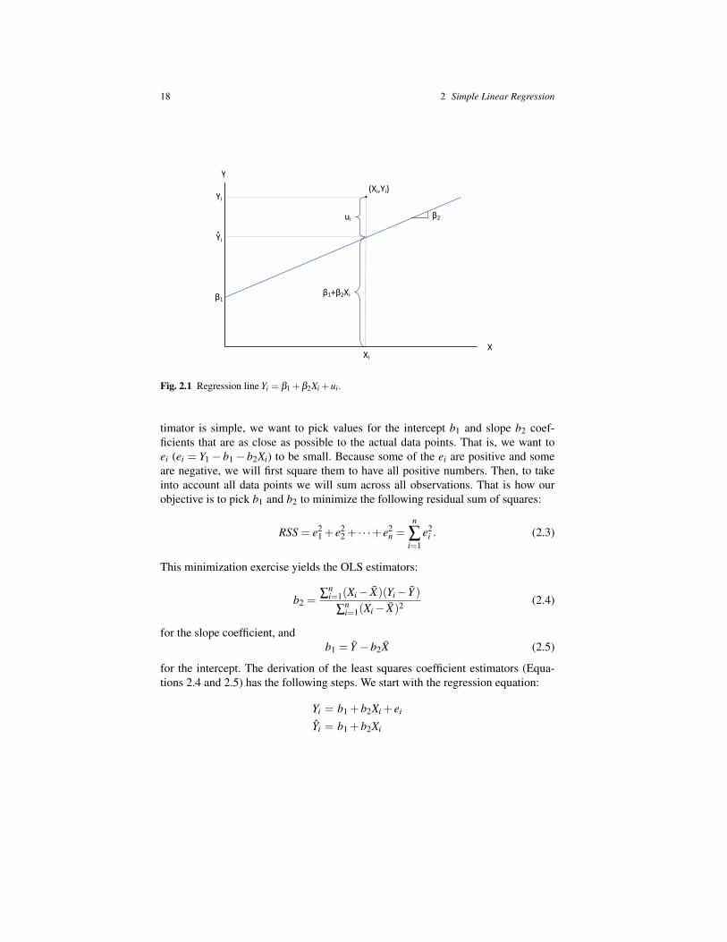
The subscript i refers to the observation i = 1,2, . . .n, and Yi is the dependent vari-able. We break down Yi into two components, the deterministic (nonrandom) com-ponent β1 +β2Xi and the stochastic (random) component ui. The explanatory vari-able is Xi and the population parameters we want to estimate are given by interceptβ1 and the slope β2. The term ui is the disturbance term. Figure 2.1 shows a graphi-cal representation of the problem. The regression line Yi = β1+β2Xi+ui is shown asthe upward sloping blue line. Only a single observation point at (Xi, Yi) is illustrated.We can see how for this observation i, we break down Yi into the disturbance termui given by the vertical distance between Yi and Yi and the height of the regressionline at point Xi, given by β1 +β2Xi.

2.2 Least squares regression

The main idea in econometric analysis is to estimate the parameters β1 and β2.The most popular estimator for these population parameters is the Ordinary LeastSquares (OLS) estimator. Let the OLS estimators of β1 and β2 be b1 and b2, respec-tively. Then, the fitter regression equation is:

Yi = b1 +b2Xi + ei. (2.2)

The difference between Equations 2.1 and 2.2 is that the first correspond to thepopulation, while the second is the sample counterpart. The idea in the OLS es-

17

18 2 Simple Linear Regression

X

Y

(Xi,Yi) Yi

Xi

Yi ^

β1

β2 ui

β1+β2Xi

Fig. 2.1 Regression line Yi = β1 +β2Xi +ui.

timator is simple, we want to pick values for the intercept b1 and slope b2 coef-ficients that are as close as possible to the actual data points. That is, we want toei (ei = Y1− b1− b2Xi) to be small. Because some of the ei are positive and someare negative, we will first square them to have all positive numbers. Then, to takeinto account all data points we will sum across all observations. That is how ourobjective is to pick b1 and b2 to minimize the following residual sum of squares:

RSS = e21 + e2

2 + · · ·+ e2n =

n

∑i=1

e2i . (2.3)

This minimization exercise yields the OLS estimators:

b2 =∑

ni=1(Xi− X)(Yi− Y )

∑ni=1(Xi− X)2 (2.4)

for the slope coefficient, andb1 = Y −b2X (2.5)

for the intercept. The derivation of the least squares coefficient estimators (Equa-tions 2.4 and 2.5) has the following steps. We start with the regression equation:

Yi = b1 +b2Xi + ei

Yi = b1 +b2Xi

2.3 Interpretation of the regression coefficients 19

For observation i we obtain the residual, then square it and finally sum across allobservations to obtain the residual sum of squares:

ei = Yi− Yi (2.6)e2

i = (Yi− Yi)2

n

∑i=1

e2i =

n

∑i=1

(Yi− Yi)2

The coefficients b1 and b2 are chosen to minimize the residuals sum of squares:

minb1,b2

∑ni=1(Yi− Yi)

2 (2.7)

minb1,b2

∑ni=1(Yi−b1−b2Xi)

2

The first order necessary condition are:

−2n

∑i=1

(Yi−b1−b2Xi) = 0 w.r.t. b1 (2.8)

−2n

∑i=1

Xi(Yi−b1−b2Xi) = 0 w.r.t. b2 (2.9)

Dividing Equation 2.9 by n and working through some math we obtain the OLSestimators for the constant:

b1 = Y −b2X .

Plugging this result into Equation 2.9 we obtain:

b2 =∑


∑ni=0(Xi− X)2 .

2.3 Interpretation of the regression coefficients

If the estimated regression equation is given by:

wagei = 4.64+0.09experi, (2.10)

where wage is the hourly wage measured in dollars, and exper is the number ofyears of experience, then the interpretation of the slope coefficient is the following:

∆wage∆exper

= 0.09.


Therefore, if the change in the number of years of experience is one, ∆exper, thenthe change in the hourly wage in dollars is given by ∆wage = 0.09. In words, anadditional year of experience will increase your hourly wage by 0.09 dollars (or 9cents). For the interpretation of the intercept, just consider the case where some-one has not experience, exper = 0. Then, this person’s predicted wage will be 4.64dollars.

If the estimated regression equation takes the form:

logwagei = 1.38+0.02experi, (2.11)

where the logwage is the natural logarithm of wage, then the interpretation is differ-ent. Here, if the number of years of experience increases by one, the wage increasesby 2% (0.02× 100 percent). Finally, for the folowing estimated equation:

logwagei = 0.98+0.26logexperi. (2.12)

A one percent increase in exper will increase wage by 0.25 percent. The 0.26 isinterpreted as an elasticity.

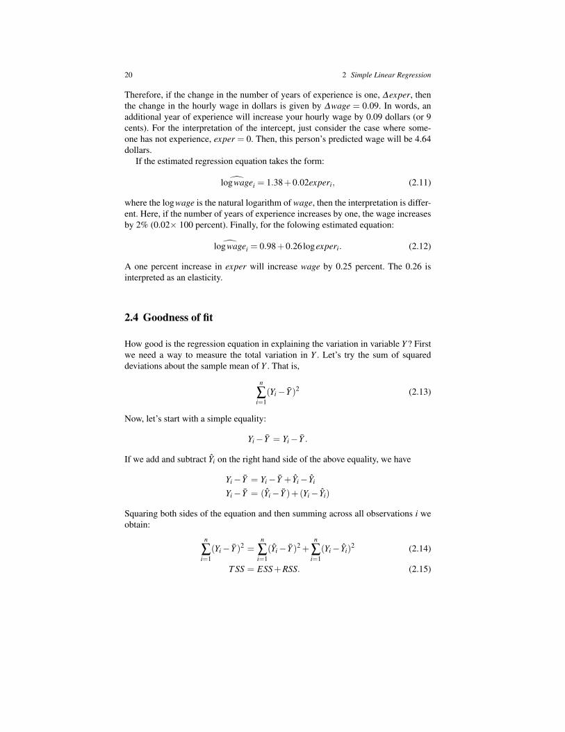
2.4 Goodness of fit

How good is the regression equation in explaining the variation in variable Y ? Firstwe need a way to measure the total variation in Y . Let’s try the sum of squareddeviations about the sample mean of Y . That is,

n

∑i=1

(Yi− Y )2 (2.13)

Now, let’s start with a simple equality:

Yi− Y = Yi− Y .

If we add and subtract Yi on the right hand side of the above equality, we have

Yi− Y = Yi− Y + Yi− Yi

Yi− Y = (Yi− Y )+(Yi− Yi)

Squaring both sides of the equation and then summing across all observations i weobtain:

n

∑i=1

(Yi− Y )2 =n

∑i=1

(Yi− Y )2 +n

∑i=1

(Yi− Yi)2 (2.14)

T SS = ESS+RSS. (2.15)

2.4 Goodness of fit 21

X

Y

(Xi,Yi) Yi

Xi

Yi ^

_

Y

_

X

Yi - Yi

Yi - Y

Yi - Yi

_

_

^

^

Fig. 2.2 Decomposition of Yi − Y .

Notice that the sum of deviations from the mean is zero, that is why there are onlytwo components on the right hand side. The T SS is the Total Sum of Squares, as pre-sented in Equation 2.13. The first term on the right hand side is ESS, the ExplainedSum of Squares, and the second term on the right hand side is the RRS, ResidualSum of Squares. This decomposition of the variable Y into two components can beappreciated in Figure 2.2. For every observation Yi in the sample, the distance be-tween Yi and Y can be decomposed in two, the part that the regression equation canexplain, Yi− Y , and the part that the regression equation cannot explain, Yi− Yi.

What is the proportion of the variation in Y that is explain by the regressionequation? We just need to divide Equation 2.15 by T SS and define the ratio of ESSto T SS as the proportion of the explained variation in Y , the R2:

1 =ESST SS

+RSST SS

(2.16)

R2 =ESST SS

= 1− RSST SS

(2.17)

R2 =∑

ni=1(Yi− Y )2

∑ni=1(Yi− Y )2 = 1− ∑

ni=1 e2

i

∑ni=1(Yi− Y )2 (2.18)

The R2 is a number between zero and one, being higher when the model explainsmore of the variation in Y . Figures 2.3 and 2.4 illustrate how the regression lineexplain the variation in Y when the R2 is low and high, respectively.


X

Y

. .

.

.

.

. .

.

.

. .

.

.

.

.

.

Low R2

Fig. 2.3 Low R2.

X

Y

.

.

. .

. . .

.

.

.

.

. .

.

. .

High R2

Fig. 2.4 High R2.

Chapter 3Properties and Hypothesis Testing

3.1 Types of data

The regression techniques developed in previous chapters can be applied to threedifferent kinds of data.

1. Cross-sectional data.2. Time series data.3. Panel data.

The first consists on observing various economic unit (e.g. firms, countries, house-holds, individuals) at one point in time. For example, we observe the wages, experi-ence and education of many individuals, only once and at all at the same time. Thesecond consists on observing the same economic unit at different point in time. Forexample, we observe daily stock prices over many years. Finally, the third combinesthe characteristics of the first and the second. That is, we observe various economicunits at repeated points in time. For example, we have information about the infla-tion, unemployment and GDP of a group of countries and over many years.

3.2 Assumptions of the model

When the regressors in our econometric model are non stochastic, we will make thefollowing six assumptions.

1. The model is linear in the parameters and it is correctly specified.

Y = β1 +β2X +u (3.1)

Y = β1Xβ2 +u (3.2)

Equation 2.1 is linear in β , while Equation 2.2 is not.

23

24 3 Properties and Hypothesis Testing

2. There is some variation in the regressor in the sample. We need variation in thevariable X to identify the relationship. Consider the OLS estimator for β2:

b2 =∑


∑ni=0(Xi− X)2 . (3.3)

If there is no variation in X , then the denominator is zero and we cannot obtainb2.

3. The expected value of the disturbance term is zero.

E(ui) = 0 for all i. (3.4)

Some ui will be negative, some will be positive, but on average they will be zero.If a constant is included in the model, the condition is satisfied automatically.

4. The disturbance term is homoscedastic.Homoscedasticity means that the variance of the error terms ui is constant acrossall observations i. Hence, we can write:

σ2ui= σ

2u for all i. (3.5)

Because the error term has zero mean (from assumption 3), then the populationvariance of ui is equal to:

E(u2i ) = σ

2u for all i. (3.6)

σ2u is a population parameter, therefore it is unknown and need to be estimated.

5. The values of the disturbance terms have independent distributions.

ui is distributed independently of u j for all j 6= i. (3.7)

This means that there is no autocorrrelation in the error term. This means thatthe population covariance between ui and u j is zero:

σuiu j = 0. (3.8)

With assumptions 1 through 5, we says that OLS coefficients are BLUE: BestLinear Unbiased Estimators. They are best, because they have the smallest vari-ance across all unbiased estimators.

6. The disturbance term has a normal distribution.

ui ∼ N[0,σ2u ] for all i. (3.9)

The error term is distributed normal with mean zero and variance σ2u . This as-

sumption becomes useful at the time of performing t tests, F tests, and construct-ing confidence intervals for β1 and β2 using the regression results. The justifica-tion for this assumption depends on the central limit theorem. This one state thatif a random variable is the composite result of the effects of a large number of

3.4 Precision of the coefficients 25

other random variables (that are not necessarily normal), it will have an approxi-mately normal distribution.

3.3 Unbiasedness of the coefficients

Recall that an estimator θ is unbiased if E(θ) = θ . The expected value of the esti-mator is equal to the true population parameter. For the slope coefficient in the OLSregression we have:

b2 =∑


∑ni=0(Xi− X)2 (3.10)

= β2 +∑

ni=0(Xi− X)ui

∑ni=0(Xi− X)2

= β2 +n

∑i=1

aiui

where

ai =(Xi− X)

∑ni=0(Xi− X)2 . (3.11)

Thus, this shows that b2 is equal to its true value, β2, plus a linear combination ofthe values of the error terms. If we take expectations of b2 we have:

E(b2) = E(β2)+E( n

∑i=1

aiui)= β2 +

n

∑i=1

E(aiui) = β2 +n

∑i=1

aiE(ui) = β . (3.12)

The term ai goes out of the expectation because ai is only a function of constantXs. In addition, the last equality holds because E(ui) = 0. Hence, b2 is an unbiasedestimator of β2, E(b2) = β2.

3.4 Precision of the coefficients

We are also interested on how precise b1 and b2 are in estimating the populationparameters β1 and β2. A measure of this precision are their population variances,given by:

σ2b1

= σ2u

(1n+

X∑

ni=0(Xi− X)2

), and (3.13)

σ2b2

=σ2

u

∑ni=0(Xi− X)2 (3.14)


One concern in the implementation of the above formulas is that σ2u is an unknown

population parameter and need to be estimated. A natural estimator for this regres-sion variance is the variance of the regression errors. Because the population regres-sion errors ui are also unknown, we use the sample counterparts ei and adjust for thecorresponding degrees of freedom. Hence, we have:

S2u =

1n−2

n

∑i=1

e2i . (3.15)

This S2u is the unbiased estimator of σ2

u , and n− 2 are the degrees of freedom. Wesubtract two from the sample size because we are estimating two parameters: theregression constant and one slope coefficient. Then, we use the following formulasto estimate the standard errors of b1 and b2:

Sb1 =

√S2

u

(1n+

X∑

ni=0(Xi− X)2

), and (3.16)

Sb2 =

√S2

u

∑ni=0(Xi− X)2 . (3.17)

3.5 The Gauss-Markov theorem

The Gauss-Markov theorem simply states that when assumptions 1 through 5 aboveare satisfied, the OLS estimators are Best Linear Unbiased Estimators (BLUE) ofthe regression parameters. Best refers to smallest variance.

3.6 Hypotheses testing

Hypothesis testing is simply a method of making decisions using data. It starts withthe formulation of the null and the alternative hypotheses and then uses some teststatistics to assess the truth of the null hypothesis.

3.6.1 Formulation of the null hypothesis

The formulation of the null hypothesis starts with a relationship in mind. For exam-ple, that the percentage rate of price inflation (p) depends on the percentage rate ofwage inflation (w) following the linear equation:

pi = β1 +β2wi +ui (3.18)

3.6 Hypotheses testing 27

Then, you want to test the hypothesis that the price inflation is equal to the wageinflation. This is denoted by H0 and it is know as the null hypothesis. In addition, wealso define an alternative hypothesis, denoted by H1 and represents the conclusion ofthe test if the null hypothesis is rejected. For our example the null and the alternativehypothesis are written as:

H0 : β2 = 1 (3.19)H1 : β2 6= 1 (3.20)

In general, the null and alternative hypotheses are:

H0 : β2 = β02 (3.21)

H1 : β2 6= β02 . (3.22)

3.6.2 t-tests

Recall that β2 is unknown and that we have to use the estimate b2. Then, the decisionrule to reject the null hypothesis should compare the estimate b2 with the hypothe-sized value β 0

2 . Intuitively, if the values are far apart, then there is evidence againstthe null. This comparison should take into account the fact that b2 is subject to somesampling variation (it is not the actual β2). We will use the following statistic:

z =b2−β 0

2σb2

(3.23)

The numerator is just the distance between the regression estimate and the hypothe-sized value, with the denominator is the standard deviation of b2, given by the squareroot of the expression in Equation 3.14. z is the number of standard deviations be-tween b2 and β2. For a known σb2 , this one follows a normal distribution. Howeverσb2 is unknown and we need to use the estimate of the standard error of b2. Thisone is given by Sb2 and it is presented in Equation 3.17. Then we use the followingt-statistic:

t =b2−β 0

2Sb2

(3.24)

To know if the deviations between b2 and β 02 are significantly large, we compare

this t-statistic with the critical values from the table t distribution with n−2 degreesof freedom. The null hypothesis is not rejected if the following condition is met:

−tn−2,α/2 ≤b2−β 0

2Sb2

≤ tn−2,α/2 (3.25)

Where tn−2,α/2 is just the notation of the critical value than comes from the t distri-bution with n− 2 degrees of freedom and at significance level α . The significance


rob

ab

ilit

y d

en

sity

Acceptance region

Reject H0 Reject H0

tp

rob

ab

ilit

y d

en

sity

t

t- t

α/2 α/2

1 - α

1 2 3 4 5 6 7 8 90 tn-2,α/2- tn-2,α/2

Fig. 3.1 Acceptance region for the t-test.

level is the probability that we reject the null hypothesis when in fact it is true. Therejection regions are illustrated in Figure 3.1.

3.6.3 Confidence intervals

The confidence interval indicates the reliability of an estimate. The confidence in-terval for the population parameter β2 can be derived from Equation 3.25 in thefollowing way:

1−α = P(− tn−2,α/2 ≤

b2−β2Sb2

≤ tn−2,α/2)

(3.26)

1−α = P(− tn−2,α/2 ·Sb2 ≤ b2−β2 ≤ tn−2,α/2 ·Sb2

)1−α = P

(b2− tn−2,α/2 ·Sb2 ≤ β2 ≤ b2 + tn−2,α/2 ·Sb2

)The meaning of the above equation is that the population parameter β2 will be be-tween the lower confidence limit b2− tn−2,α/2 · Sb2 and the upper confidence limitb2+tn−2,α/2 ·Sb2 with probability (1−α) or 100×(1−α)%. The p values provide analternative approach to reporting the significance of regression coefficients or whencarrying out more general hypothesis testing. As you can see from Equation 3.25and Figure 3.1, different significance levels α can yield a different conclusion in therejection or not of the null hypothesis. The p value of a hypothesis test represent theminimum significance level at which the null is rejected. Then, when the p value isbelow the significance level α we reject the null.

3.6 Hypotheses testing 29

rob

ab

ilit

y d

en

sity

100·(1 - α)% Confidence Interval

b2

pro

ba

bil

ity

de

nsi

ty

b2

bb - t ·S

α/2 α/2

1 - α

b + t ·S1 2 3 4 5 6 7 8 9b2b2 - tn-2,α/2·Sb2

b2 + tn-2,α/2·Sb2

Fig. 3.2 Confidence interval for β2.

3.6.4 F test

A useful tool if we want to test if there is no relationship between X and Y if the Ftest. In the simple linear regression model with only one slope coefficient, the nulland the alternative in an F test are:

H0 : β2 = 0 (3.27)H1 : β2 6= 0. (3.28)

This test is build on the idea of testing how good is the regression model in explain-ing the variation in Y . In Equation 2.15 we already separated the variation of Y intoits ‘explained’ and ‘unexplained’ components. These are:

n

∑i=1

(Yi− Y )2 =n

∑i=1

(Yi− Y )2 +n

∑i=1

(Yi− Yi)2 (3.29)

T SS = ESS+RSS. (3.30)

The total sum of squares (TSS) is the summation of the explained sum of squares(ESS) and the residual sum of squares (RSS). Then, the F statistic for goodness of fitof a regression is written as the explained sum of squares, per explanatory variable,divided by the residual sum of squares, per remaining degrees of freedom:

F =ESS/(k−1)RSS/(n− k)

(3.31)


SUMMARY OUTPUT

Regression Statistics

Multiple R 0.2346

R Square 0.0551

Adjusted R Square 0.0543

Standard Error 4.5323

Observations 1260

ANOVA

df SS MS F Significance F

Regression 1 1505.5387 1505.5387 73.2906 0.0000

Residual 1258 25841.9006 20.5421

Total 1259 27347.4393

Coefficients Standard Error t Stat P-value Lower 95% Upper 95%

Intercept 4.6425 0.2326 19.9615 0.0000 4.1862 5.0988

X Variable 1 0.0914 0.0107 8.5610 0.0000 0.0705 0.1124

Fig. 3.3 Regression output in MS Excel.

where k is the total number of coefficients we are estimating, hence (k− 1) is thenumber of slope coefficients. That is, the total number of parameters we are estimat-ing minus the constant parameter. If we divide the numerator and the denominatorby T SS, then the F statistics can be written in terms of the R2 as follows:

F =(ESS/T SS)/(k−1)(RSS/T SS)/(n− k)

=R2/(k−1)

(1−R2)/(n− k)(3.32)

If this F statistic is greater that the critical value from the table F distribution with(k− 1) and (n− k) degrees of freedom, Fk−1,n−k, we reject the null hypothesis andconclude that the regression model does not significantly explain the variation invariable Y . For the simple regression model with only one slope coefficient, k = 2,we have:

F =R2

(1−R2)/(n−2). (3.33)

If this F statistic > F1,n−2 we reject the null hypothesis presented in Equation 3.28.

3.7 Computer output 31

3.7 Computer output

The computer regression output is very similar across different statistical packages.Figure 3.3 shows the output using MS Excel for the estimation of the followingsimple regression model:

wage=β1 +β2experi +ui (3.34)

To obtain the regression estimated coefficients we use Equations 2.4 and 2.5:

b2 =∑


∑ni=1(Xi− X)2 = 0.091 (3.35)

b1 = Y −b2X = 4.642 (3.36)

The total sum of squares, estimates sum of squares, and residual sum of squares areobtained using 2.15 and 2.15:

T SS =n

∑i=1

(Yi− Y )2 = 27347.439 (3.37)

ESS =n

∑i=1

(Yi− Y )2 = 1505.539 (3.38)

RSS =n

∑i=1

(Yi− Yi)2 = 25841.901 (3.39)

The regression R2 comes from Equation 2.18:

R2 = 1− ∑ni=1 e2

i

∑ni=1(Yi− Y )2 = 0.055 (3.40)

From the square root of Equation 3.15:

Su =

√1

n−2

n

∑i=1

e2i = 4.532 (3.41)

Then, the standard errors of the coefficients are computer using Equations 3.17and 3.17:

Sb1 =

√S2

u

(1n+

X∑

ni=0(Xi− X)2

)= 0.233 (3.42)

Sb2 =

√S2

u

∑ni=0(Xi− X)2 = 0.011 (3.43)

The F statistic uses Equation 3.32:


F =R2/(k−1)

(1−R2)/(n− k)= 73.291 (3.44)

The t statistics use Equation 3.24:

t =b1

Sb1

= 19.961 (3.45)

t =b2

Sb2

= 8.561 (3.46)

Finally, for the 95% upper and lower confidence levels, we use Equation 3.26:

b1− tn−2,α/2 ·Sb1 = 4.186 (3.47)b1 + tn−2,α/2 ·Sb1 = 5.099 (3.48)b2− tn−2,α/2 ·Sb2 = 0.071 (3.49)b2 + tn−2,α/2 ·Sb2 = 0.112 (3.50)

Chapter 4Multiple Regression Analysis

The simple linear regression covered in Chapter 2 can be generalized to includemore than one variable. Multiple regression analysis is an extension of the simpleregression analysis to cover cases in which the dependent variable is hypothesizedto depend on more than one explanatory variable. While much of the analysis is anextension of the simple case, we have two main complications. (1) We need to dis-criminate between the effects of one variable and the effects of the other explanatoryvariables. (2) We have to decide which variables to include in the regression equa-tion. In this chapter we will focus on the extension of the linear regression modeland in (1). In a later chapter we will discuss (2).

4.1 Interpretation of the coefficients

Consider the following population multiple regression model with (k− 1) regres-sors:

Y = β1 +β2X2 +β3X3 + · · ·+βkXk +u. (4.1)

A simple example of a multiple regression model is:

CRIMEi = β1 +β2POPULAT IONi +β3UNEMPLOYi +β4POLICEi +ui, (4.2)

where i refers to the city, CRIME is crime rates, POPULAT ION is just the numberpeople in city i, UNEMPLOY is the unemployment rate, and POLICE is the num-ber of police officers. To estimate the β s in Equation 4.2 you may need to observecrime rates and all the other variables for n cities. As before, u is the disturbanceterm. Because we have more that one regressor, the simple two dimensional charac-terization illustrated in Figure 2.1 is no longer applicable. Now, we have a (k− 1)dimensional problem. In our crime example we would need to have a 4D graph!

The sample counterpart of Equation 4.2 is:

CRIMEi = b1 +b2POPULAT IONi +b3UNEMPLOYi +b4POLICEi + ei, (4.3)

33

34 4 Multiple Regression Analysis

where the bs are the sample estimates of the β s, and are estimated using computersoftware via Ordinary Least Squares. We also express this relationship as the 4Dfitted plane:

CRIME i = b1 +b2POPULAT IONi +b3UNEMPLOYi +b4POLICEi. (4.4)

Notice that we no longer write the disturbance term. Moreover, CRIME i is the fittedor predicted value of CRIMEi. The interpretation of the coefficients is the same asbefore. If the number of police officers increases by one, then the crime rate willchange by b4. Similar interpretation follows for b2 and b3.

4.2 Ordinary Least Squares

The OLS estimates are obtained in the same fashion as before. The unknown rela-tionship is given by:

Yi = β1 +β2X2i +β3X3i + · · ·+βkXki +ui. (4.5)

The fitted OLS regression is:

Yi = b1 +b2X2i +b3X3i + · · ·+bkXki. (4.6)

Then, the OLS regression residuals are:

ei = Yi− Y = Yi−b1−b2X2i−b3X3i−·· ·−bkXki. (4.7)

Recall that OLS minimizes the sum of squared residuals

minb1,b2,...,bk

∑ni=1(Yi− Yi)

2, (4.8)

where RSS = ∑ni=1(Yi− Yi)

2 is the sum of squared residuals. We need to take thederivative of the RSS with respect to b1, b2, . . . , bk and obtain k first order conditions.This yields a system of k equations with k unknowns, where the solution is the OLSestimators of the β s.

4.3 Assumptions

1. The model is linear in the parameters and correctly specified

Y = β1 +β2X2 +β3X3 + · · ·+βkXk +u. (4.9)

4.4 Properties of the coefficients 35

2. There is no exact linear relationship among the regressors in the sample. This iscalled multicollinearity.

3. The disturbance term has expectation zero

E(ui) = 0 for all i. (4.10)

4. The disturbance term is homoscedastic.

σ2ui= σ

2u for all i. (4.11)

5. The values of the disturbance term have independent distributions.

ui is distributed independently of ui′ for all i′ 6= i. (4.12)

6. The distribution term has a normal distribution.

ui ∼ N[0,σ2] for all i. (4.13)

All the Xs are nonstochastic.

4.4 Properties of the coefficients

4.4.1 Unbiasedness

The OLS estimator b j of β j is unbiased:

E(b j) = β j (4.14)

4.4.2 Efficiency

Following the results from the Gauss-Markov theorem, we have that OLS yields themost efficient linear estimators, in the sence that they are the one with the smallestvariance among all linear estimators.

4.4.3 Precision of the coefficient, t tests, and confidence intervals

Beside our interest on the point estimates, we are also interested in performing hy-potheses testing and building confidence intervals. To do this we need a measure ofthe precision of the coefficients. While we will not show the derivation here (as itrequired matrix algebra), each of the b j has an standard error, Sb j .


The null and alternative hypotheses about population coefficient j is written as:

H0 : β j = β0j (4.15)

H1 : β j 6= β0j . (4.16)

which can be tested using the following t-statistic:

t =b j−β 0

j

Sb j

(4.17)

The null is not rejected if the following condition is met:

−tn−k,α/2 ≤b j−β 0

j

Sb j

≤ tn−k,α/2 (4.18)

Notice the difference between Equation 4.18 and Equation 3.25. The critical valuefrom the t distribution, tn−k,α/2, now has n− k degrees of freedom because we areestimating k parameters, rather than just 2 as in the simple regression model. Theintuition behind Figures 3.1 and 3.1 still hold. The computer software will also giveyou the p-value associated with the t test. If the p-value is below your α , you rejectthe null hypothesis.

For the construction of the confidence intervals we have:

1−α = P(− tn−k,α/2 ≤

b j−β jSb j

≤ tn−k,α/2)

(4.19)

1−α = P(− tn−k,α/2 ·Sb j ≤ b j−β j ≤ tn−k,α/2 ·Sb j

)1−α = P

(b j− tn−k,α/2 ·Sb j ≤ β j ≤ b j + tn−k,α/2 ·Sb j

).

4.5 Regression output in Gretl

Gretl is an open-source (free) software package for econometric analysis written inthe C programming language. It can be downloaded from:

http://gretl.sourceforge.net/

Just follow the instructions to install it in your computer.Once you loaded the data set in Gretl, to estimate Equation 4.2 you need to go to

Model→ Ordinary Least Squares. The regression output is:

4.6 Multicollinearity 37

Model 1: OLS, using observations 1-92Dependent variable: crimes

coefficient std. error t-ratio p-value-----------------------------------------------------------const 2193.34 3918.06 0.5598 0.5770pop 0.0652716 0.0106262 6.143 2.30e-08 ***unem -279.291 407.791 -0.6849 0.4952officers 15.0406 3.57660 4.205 6.25e-05 ***

Mean dependent var 39663.53 S.D. dependent var 29692.10Sum squared resid 1.39e+10 S.E. of regression 12548.04R-squared 0.827293 Adjusted R-squared 0.821405F(3, 88) 140.5107 P-value(F) 1.90e-33Log-likelihood -996.7310 Akaike criterion 2001.462Schwarz criterion 2011.549 Hannan-Quinn 2005.533

Excluding the constant, p-value was highest for variable 3 (unem)

A standard way to present the regression output is:

crimes = 2193.34(3918.1)

−279.291(407.79)

unem+15.0406(3.5766)

officers+0.0652716(0.010626)

pop

N = 92 R2 = 0.8214 F(3,88) = 140.51 σ = 12548.(standard errors in parentheses)

To obtain the confidence intervals for the coefficients as presented in Equa-tion 4.19 in the Gretl regression output window you need to go to Analysis →Confidence intervals for the coefficients to obtain:

t(88, 0.025) = 1.987

VARIABLE COEFFICIENT 95% CONFIDENCE INTERVAL

const 2193.34 -5592.97 9979.66pop 0.0652716 0.0441542 0.0863890

unem -279.291 -1089.69 531.107officers 15.0406 7.93282 22.1483

4.6 Multicollinearity

Multicollinearity is when two explanatory variables are highly correlated. In addi-tion, if their coefficients have a large population variances, we are at risk of gettingerratic estimates of the coefficients. There could also be multicollinearity when thereis an approximate linear relationship between more than two variables.

A simple test for multicollinearity is based in the Variance Inflation Factors.To implement this text in Gretl, in the regression output window go to Test →Collinearity:

Variance Inflation Factors


Minimum possible value = 1.0Values > 10.0 may indicate a collinearity problem

pop 4.180unem 1.094

officers 4.371

VIF(j) = 1/(1 - R(j)ˆ2), where R(j) is the multiple correlationcoefficient between variable j and the other independent variables

Properties of matrix X’X:

1-norm = 2.0266173e+013Determinant = 6.6859257e+024Reciprocal condition number = 4.681685e-013

Based on these results, we do not have a multicollinearity problem in the estimationof Equation 4.2.

4.7 Goodness of fit: R2 and R2

The R2 in multiple regression analysis has the same interpretation as in a simpleregression. It is the proportion of the variation in Y explained by the regressionmodel

R2 =ESST SS

= 1− RSST SS

(4.20)

R2 =∑

ni=1(Yi− Y )2

∑ni=1(Yi− Y )2 = 1− ∑

ni=1 e2

i

∑ni=1(Yi− Y )2 (4.21)

where Y represents the fitted values of the regression equation

Y = b1 +b2X2 +b3X3 + · · ·+bkXk. (4.22)

4.8 F tests

Given the population regression model

Y = β1 +β2X2 +β3X3 + · · ·+βkXk +u, (4.23)

we can use the F test to test if all the slope coefficients β2,β3, . . . ,βk are jointlyequal to zero. That is, let the null hypothesis be:

H0 : β2 = β3 = · · ·= βk = 0. (4.24)

4.9 Adjusted R2, R2 39

The alternative hypothesis (H0) is that at least one of the slope coefficients is differ-ent from zero. The multiple regression version of the F statistic is:

Fk−1,n−k =ESS/(k−1)RSS/(n− k)

. (4.25)

The idea is to compare this F statistic to the critical level found in the F distributiontables with k− 1 and n− k degrees of freedom. Computer software automaticallycomputes this F statistic and the corresponding p-value for the null in Equation 4.22.This F statistic can also be written in terms of the R2:

Fk−1,n−k =R2/(k−1)

(1−R2)/(n− k). (4.26)

Consider the example presented in Section 4.5. The F statistic is 140.5107 with 3and 88 degrees of freedom and has a corresponding p-value of 0.000. Then, be-cause the p-value is below α = 5% then we reject the null hypothesis that the slopecoefficients on pop, unem, and officers are jointly equal to zero.

4.9 Adjusted R2, R2

One concern with the R2 is that it will always go up as we include more variablesinto the model. Hence, it is a poor way to compare models. On the other hand asimilar statistic, the adjusted R2 (R2) is built on the R2 but with the difference thatR2 penalizes for the loss of the degrees of freedom as we include more variables intothe model. Therefore, the R2 can either go up or down as we include more variableinto the model. It is defined as:

R2 = R2− k−1n− k

(1−R2). (4.27)

Chapter 5Transformations of Variables and Interactions

5.1 Basic idea

One limitation in the linear regression analysis is that the dependent variable has tobe linear in the parameters:

Y = β1 +β2X2 +β3X3 + · · ·+βkXk +u. (5.1)

However, there are equations that are not linear, for example:

Y = β1 +β2X2 +Xβ33 +u. (5.2)

This Equation 5.2 cannot be estimated using OLS. One way to estimate nonlinearmodels is by using Nonlinear Least Squares (NLS), which is an extension of themethods we discussed before. In this chapter, rather that focusing on NLS, we willsee how transformations in the variables can allow us to use OLS on a variety of non-linear models. For example, consider the estimation of the following Cobb-Douglasproduction function:

Pi = ALβ2i Kβ3

i eεi , (5.3)

where Pi is total production or total output, A is a technology constant, Ki is theamount of capital, and Li is labor. Taking natural logs we have:

logPi = logA+β2 logLi +β3 logKi + εi. (5.4)

If we simple set Yi = logPi, β1 = logA, X2 = logLi, and X3 = logKi we can writeEquation 5.4 as:

Yi = β1 +β2X2i +β3X3i + εi, (5.5)

that can be easily estimated via OLS. β2 and β3 will correspond to the ones given inEquation 5.3. Another example of a model that can be estimated with OLS is:

Yi = β1 +β2Z22i +β3

√Z3i +β4

1Z4i

+ εi. (5.6)

41

42 5 Transformations of Variables and Interactions

We just need to replace X2i = Z22i, X3i =

√Z3i, X4i =

1Z4i

.

5.2 Logarithmic transformations

To explain the logarithm transformation let’s go over one example in Gretl. If wewant to estimate the following model:

logcrimei = β1 +β2 logpopi +β3unemi +β4offii +ui, (5.7)

you need to create the new variables first. Go to Add→ Define new variableand type:

logcrime = log(crime)

This will generate the new variable logcrime. Do the same thing for log popula-tion and then estimate the model. The regression output is:

Model 1: OLS, using observations 1-92Dependent variable: logcrime

coefficient std. error t-ratio p-value-----------------------------------------------------------const -0.709735 0.807193 -0.8793 0.3817unem -0.00456848 0.00903041 -0.5059 0.6142offi 0.000144915 6.15429e-05 2.355 0.0208 **logpop 0.864044 0.0662782 13.04 2.92e-022 ***

Mean dependent var 10.33774 S.D. dependent var 0.742056Sum squared resid 6.883563 S.E. of regression 0.279683R-squared 0.862628 Adjusted R-squared 0.857945F(3, 88) 184.1989 P-value(F) 8.20e-38Log-likelihood -11.28034 Akaike criterion 30.56069Schwarz criterion 40.64784 Hannan-Quinn 34.63195

Excluding the constant, p-value was highest for variable 3 (unem)

logcrime=−0.709735(0.80719)

−0.00456(0.00903)

unem+0.000144915(6.1543e–005)

offi+0.8640(0.0663)

logpop

N = 92 R2 = 0.8579 F(3,88) = 184.20 σ = 0.27968(standard errors in parentheses)

First, notice how the coefficients are very different from the one obtain with nologarithm transformation. Here the interpretation is different. β2 is interpreted as theelasticity of crime with respect to pop:

β2 =∆crime/crime

∆pop/pop. (5.8)

5.3 Quadratic terms 43

A one percentage increase in popwill increase crime by 0.864 percent. ∆crime/crimeis interpreted as a percentage change in crime. For β4 we have:

β4 =∆crime/crime

∆offi. (5.9)

Here, a one unit increase in offi is associated with a 0.014% (0.00014 × 100percent) increase in crime.

5.3 Quadratic terms

So far we have bee estimating the marginal effects (β s) that are constant across allpossible values of X . The simplest way to introduce nonlinearities in the marginaleffect is to estimate the model with quadratic terms. For example, let the model be:

Yi = β1 +β2Xi +β3X2i + εi. (5.10)

In this case the marginal effect of X on Y is given by:

∆Y∆X

= β2 +2 ·β3Xi. (5.11)

If we want to estimate the marginal effect of experience of wages and in additionwe allow for a nonlinear effect we can estimate:

wagei = β1 +β2experi +β3expersqi + εi, (5.12)

where wage is average hourly earnings, exper is years of experience and expersqis the number of years of experience squared. The Gletl output is the following:

Model 1: OLS, using observations 1-526Dependent variable: wage

coefficient std. error t-ratio p-value----------------------------------------------------------const 3.72541 0.345939 10.77 1.46e-024 ***exper 0.298100 0.0409655 7.277 1.26e-012 ***expersq -0.00612989 0.000902517 -6.792 3.02e-011 ***



05

10

15

20

25

0 10 20 30 40 50exper

95% CI Fitted values

wage

Fig. 5.1 Predicted values for Equation 5.12

wage= 3.72541(0.34594)

+0.298100(0.040966)

exper−0.00612989(0.00090252)

expersq


Here, the marginal effect of experience on average hourly wage is:

∆wage

∆exper= 0.2981+2 · (−0.006)exper

= 0.2981−0.012exper.

For a person with 2 years of experience, the effect of an additional year of experienceon wage is 0.2741 (=0.2981 - 0.012 × 2) and for a person with 15 years of expe-rience, the marginal effect of an additional year of experience is 0.1181 (=0.2981 -0.012 × 15). Hence, we can say that for a reasonable range of years of experience,experience has a positive effect on wage. In addition, this effect is smaller as youaccumulate more experience.

Figure 5.1 show the fitted regression line along with the 95% confidence intervalfor the fitted values and the actual data. This figure clearly shows the nonlinearmarginal effect and innlustrates how wages increase with experience for about thefirst 25 years, but then wages decrease later on.

5.4 Interaction terms 45

5.4 Interaction terms

A second popular approach to allow for the marginal effect to change over differentvalues of X is to include interaction terms in the regression equation. For example,

Y = β1 +β2X2 +β3(X2×X3)+ εi. (5.13)

In this case the marginal effect of X2 on Y depends on X3 is given by:

∆Y∆X2

= β2 +β3X3. (5.14)

Consider the next example with the interaction between exper and educ in a wageequation:

wagei = β1 +β2experi +β3(experi×educi)+ εi, (5.15)

where the marginal effect of experience on wage depends on the level of education:

∆wage

∆exper= β2 +β3educ. (5.16)

When estimating this equation in Gretl we have to make sure we generate the inter-action term first. That is, go to Add→ Define new variable and type:

expereduc = exper*educ

Then we are ready to estimate the equation via OLS. The regression output is:


coefficient std. error t-ratio p-value----------------------------------------------------------const 4.88993 0.242730 20.15 3.11e-067 ***exper -0.188124 0.0253904 -7.409 5.13e-013 ***expereduc 0.0207731 0.00217625 9.545 5.17e-020 ***


wage= 4.88993(0.24273)

−0.188124(0.025390)

exper+0.0207731(0.0021762)

expereduc



Here, the marginal effect of experience on wage is:

∆wage

∆exper= −0.1881+0.0208educ

For a person with twelve years education (high school), the marginal effect from anadditional year of education is 0.0615 (=-0.1881+0.208×12). However, with moreeducation the marginal effect is larger. A person with 16 years of education (highschool + college) will have a marginal effect of 0.1447 (=-0.1881+0.208×16). No-tice that for an important range of education the marginal effect is positive, meaningthat more experience leads to higher wages. In addition, the effect if larger if youhave more education. This means that going to school is not only good because itdirectly increases your expected wage but also makes additional years of experiencemore valuable.

Chapter 6Analysis with Qualitative Information: DummyVariables

In previous chapters, the dependent and the independent variables in our regressionequations had a quantitative meaning. That is, the magnitude of the variable hada useful information, for example, years of education, years of experience, unem-ployment rate, or wage. In this chapter we will analyze how to introduce qualitativeinformation into a regression equation. Example of qualitative information includesmarital status, gender, race, industry (manufacturing, retail, etc.) or geographicalregion (south, north, west, etc.).

6.1 Describing qualitative information

Qualitative factors often come in the form of binary information: a person is femaleof male; a person does or does not own a computer; a person is married or not. Inall these cases the relevant information can be captured by a binary variable, alsocalled a dummy variable or zero-one variable. In defining a dummy variable we mustdecide which event is assigned a value of one and which a value of zero. Table 6.1shows how two dummy variables (female and married) look in the data set.

Table 6.1 A partial Listing of the Data in Wage.xls

person wage educ exper female married1 3.10 11 2 1 02 3.24 12 22 1 13 3.00 11 2 0 04 6.00 8 44 0 15 5.30 12 7 0 1...

......

......

...525 11.56 16 5 0 1526 3.50 14 5 1 0

47

48 6 Analysis with Qualitative Information: Dummy Variables

Fig. 6.1 Graph of wage= β0 +δ0female+β1educ for δ0 < 0.

6.2 A single dummy independent variable

The simplest case is when we have a single dummy independent variable. Let’sconsider the following model:

wage= β0 +δ0female+β1educ+ ε (6.1)

We use the parameter δ0 to emphasize the fact that female corresponds to adummy variable. If the person is a female we have female = 1, and if the person isa male, we have female = 0. The parameter δ0 has the following interpretation: δ0is the difference in hourly wage between females and males, given the same amountof education (and the error term ε). Thus, the coefficient δ0 determines whetherthere is discrimination against women: if δ0 < 0, it means that on average, womenearn less than men.

The interpretation of δ0 (when δ < 0) can be depicted graphically in Figure 6.1as an intercept shift between males an females.

Let’s estimate the following more interesting model:

wage= β0 +δ0female+β1educ+β2exper+β1tenure+ ε (6.2)

The regression output in Gretl is:


6.2 A single dummy independent variable 49

coefficient std. error t-ratio p-value---------------------------------------------------------const -1.56794 0.724551 -2.164 0.0309 **female -1.81085 0.264825 -6.838 2.26e-011 ***educ 0.571505 0.0493373 11.58 9.09e-028 ***exper 0.0253959 0.0115694 2.195 0.0286 **tenure 0.141005 0.0211617 6.663 6.83e-011 ***


wage=−1.56794(0.72455)

−1.81085(0.26483)

female+0.571505(0.049337)

educ+0.0253959(0.011569)

exper

+0.141005(0.021162)

tenure


Where it is easy to see that δ0 = −1.81. If we want to test the null hypothesisthat there is no difference between men and women, H0 : δ0 = 0. The alternativehypothesis is that there is discrimination against women, H1 : δ0 < 0. Based on thep-value we reject the null and conclude that there is discrimination, females maketwo dollars and twenty seven cents less per hour than males. This is after controllingfor differences in education, experience and tenure.

It is illustrative to additionally estimate the following equation:

wage= β0 +δ0female+ ε (6.3)

where we do not control for education, experience or tenure. The regression outputis:


coefficient std. error t-ratio p-value---------------------------------------------------------const 7.09949 0.210008 33.81 8.97e-134 ***female -2.51183 0.303409 -8.279 1.04e-015 ***



wage= 7.09949(0.21001)

−2.51183(0.30341)

female


The expected (predicted) wage for females is wage = 7.099− 2.5121 = 4.587,while the expected wage for males is wage= 7.099−2.5120= 7.099. This is notcontrolling for differences in education, experience or tenure. Once we control forthose differences, the wage gap between these two groups is smaller and equal toδ0 =−1.81.

What is the interpretation of the coefficient on a dummy variable if the dependentvariable is in logs? Here the coefficient has a percentage interpretation. Let’s say wewant to estimate the following equation:

logwage= β0 +δ0female+β1educ+β2exper+β3tenure+ ε (6.4)

that has the following Gretl estimation output:

logwage= 0.501348(0.10190)

−0.301146(0.037246)

female+0.0874623(0.0069389)

educ+0.00462938(0.0016271)

exper

+0.0173670(0.0029762)

tenure


The coefficient on female, δ0, implies that for the same levels of education, expe-rience, and tenure, women earn approximately 100(0.301) = 30.1% less than men.

6.3 Dummy variables for multiple categories

One can use several dummy variables in the same equation. For example, we canadd the dummy variable married to Equation 6.3 to obtain:

wage= β0 +δ0female+δ1married+ ε (6.5)

In Gretl we have,

wage= 6.18043(0.29634)

−2.29440(0.30261)

female+1.33948(0.30971)

married


The coefficient on married gives the (approximate) difference in wages betweenmarried and non married individuals. Based on these results, married individuals

6.4 Incorporating ordinal information 51

have higher hourly wages. On important restriction in Equation 6.5 is that it restrictsthe effect of marital status on wages is the same whether you are male of female.If we are interested in this difference we can estimate an alternative model withadditional categories. In particular we need four categories: (1) married men, (2)married women (3) single men, and (4) single woman. We must select a base group(for example, single men) and create the dummy variables for the other three groups.

marrmale = married× (1−female)marrfem = married×femalesingfem = (1−married)×female

The equation we want to estimate is:

logwage= β0 +δ0marrmale+δ1marrfem+δ2singfem+ ε (6.6)

and the estimation output is:

logwage= 1.5201(0.050987)

+ 0.4267(0.061554)

marrmale− 0.0797(0.065524)

marrfem− 0.1316(0.066804)

singfem


The interpretation of each of the δ coefficients is with respect to the base group. Forexample δ2 = 0.1316 means that single females earn approximately 13.16% lowerhourly wages than single men (the base group).

6.4 Incorporating ordinal information

Suppose we want to estimate the effect of city credit ratings on the municipal bondinterest rate (MBR). The credit rating (CR) is an ordinal variable and suppose it goesfrom zero (worst credit) to four (best credit). Under these consideration, a potentialcandidate for our model is:

MBR= β0 +β1CR+other f actors+ ε (6.7)

where other f actors are just other variables in the model. On concern with this spec-ification is that it is hard to interpret one unit increase in CR. It is easy to talk aboutan additional year of education or an additional year of income, but credit ratingsusually have only an ordinal meaning. Moreover, it is restrictive to assume that eachadditional unit increase in CR has the same effect on MBR. An alternative approachis to create separate dummy variables for each of the values of CR, that is,


CR1 = 1 if CR= 1= 0 otherwise.




Then we can focus on estimating the following model:

MBR= β0 +δ1CR1 +δ2CR2 +δ3CR3 +other f actors+ ε (6.8)

Again, we omit one category (CR4) and the interpretation of the dummy coefficientsis relative to the omitted category. For example, δ2 represents the difference in mu-nicipal bond interest rate between ratings CR2 and CR4.

6.5 Interactions involving dummy variables

Just as quantitative variables can have interactions, so can dummy variables. Actu-ally, we revisit the estimation of Equation 6.6 to see that the same results can beachieved by including the interaction term between female and married. Themodel we want to estimate is:

logwage= β0+δ0female+δ1married+δ2(female×married)+ε (6.9)

Estimating in Gretl we have:

logwage= 1.5201(0.050987)

− 0.1316(0.066804)

female+ 0.4267(0.061554)

married

− 0.3748(0.085708)

female×married


Notice that this regression output is equivalent as the one obtained from Equa-tion 6.6.

6.5 Interactions involving dummy variables 53

Fig. 6.2 Graph of wage= β0 +δ0female+β1educ+δ1educ×female.

6.5.1 Allowing for different slopes

Consider the case where we want to estimate the effect of education on hourly wageand in addition, we want for the marginal effect to change based on your gender.This can be done by interacting the educ with female and estimating the follow-ing model:

wage= β0 +δ0female+β1educ+δ1(female×educ)+ ε (6.10)

A graphical approach to this problem in presented in Figure 6.2. The output in Gretlis

wage= 0.200496(0.84356)

−1.19852(1.3250)

female+0.539476(0.064223)

educ

−0.0859990(0.10364)

female×educ

T = 526 R2 = 0.2555 F(3,522) = 61.070 σ = 3.1865(standard errors in parentheses)


6.5.2 Testing for differences in regression functions across groups

So far we saw that interacting a dummy variable with other independent variablesis a powerful tool. Now, we can use this tool to test the null hypothesis that twogroups follow the same regression function, against the alternative that one or moreof the slopes differs across the two groups. Suppose we want to test whether thesame regression model describe college GPA for males and for females. The modelis

cumgpa= β0 +β1sat+β2hsperc+β3tothrs+ ε, (6.11)

where cumgpa is cumulative college GPA, sat is the SAT score, hsperc is thehigh school rank percentile, and tothrs is the total hours of college courses. Theregression results in Gretl are

cumgpa= 0.929111(0.22855)

+0.0009028(0.000208)

sat−0.006379(0.00157)

hsperc+ 0.01198(0.000931)

tothrs


To allow for a difference in the intercept we just need to include the dummy variablefemale. Then, to allow differences in the slope parameters we need to includeinteraction terms for each of the variables and female. That is

cumgpa = β0 +δ0female+β1sat+δ1sat ·female (6.12)+ β2hsperc+δ2hsperc ·female+ β3tothrs+δ3tothrs ·female+ ε

The parameter δ0 is the difference in the intercepts between females and males, δ1is the slope difference with respect to sat between females and males, and so on.The null hypothesis that cumgpa follows the same model for females and males is

H0 : δ0 = δ1 = δ2 = δ3 = 0 (6.13)

If at least one of the δ j is different from zero, then the model is different for menand women. After creating the interaction terms, the estimated model in Gretl is

Model 2: OLS, using observations 1-732Dependent variable: cumgpa

coefficient std. error t-ratio p-value----------------------------------------------------------------const 1.21398 0.264828 4.584 5.37e-06 ***sat 0.000611312 0.000235026 2.601 0.0095 ***hsperc -0.00596745 0.00177646 -3.359 0.0008 ***tothrs 0.0103004 0.00109284 9.425 5.65e-020 ***female -1.11364 0.528539 -2.107 0.0355 **satfemale 0.00111674 0.000500034 2.233 0.0258 **hspercfemale 5.07597e-05 0.00410253 0.01237 0.9901tothrsfemale 0.00555989 0.00206958 2.686 0.0074 ***

6.5 Interactions involving dummy variables 55


cumgpa= 1.21398(0.26483)

+0.000611312(0.00023503)

sat−0.00596745(0.0017765)

hsperc+0.0103004(0.0010928)

tothrs

−1.11364(0.52854)

female+0.00111674(0.00050003)

satfemale+5.07597e–005(0.0041025)

hspercfemale

+0.00555989(0.0020696)

tothrsfemale


Now, to test the null hypothesis presented in Equation 6.13 from the window thatshows the regression output, we need to go to Tests→ Omit variables anda new window will open. We then have to select the variables to omit. There arefemale, satfemale, hspercfemale, and tothrsfemale. This will esti-mate the restricted model and the comparison between the restricted model (Equa-tion 6.11) and the full model (Equation 6.12),


coefficient std. error t-ratio p-value-----------------------------------------------------------const 0.929111 0.228552 4.065 5.32e-05 ***sat 0.000902834 0.000207870 4.343 1.60e-05 ***hsperc -0.00637913 0.00156785 -4.069 5.24e-05 ***tothrs 0.0119779 0.000931383 12.86 2.96e-034 ***


Comparison of Model 2 and Model 3:

Null hypothesis: the regression parameters are zero for the variablesfemale, satfemale, hspercfemale, tothrsfemale

Test statistic: F(4, 724) = 4.4227, with p-value = 0.00154347Of the 3 model selection statistics, 1 has improved.

The F statistics that Gretl is reporting comes from


F =RSS−RSSUR

RSSUR· n−2k

q, (6.14)

where RSS is the residual sum of squares of the model estimates in Equation 6.11and RSSUR is the unrestricted model in Equation 6.12. n is the sample size, k is thenumber of parameters we are estimating, and q is the number of restrictions whencomparing the model in Equation 6.11 and in Equation 6.12. Substituting the valueswe obtain,

F =547.3649−534.3092

534.3092· 732−2 ·4

4= 0.024434 ·181 = 4.4227, (6.15)

An alternative way to calculate this F statistic is to follow the formula,

F =RSS− (RSS1 +RSS2)

RSS1 +RSS2· n−2k

k, (6.16)

where RSS is the residual sum of squares of the model estimates in Equation 6.11.RSS1 and RSS2 are the residual sum of squares of the model estimated in Equa-tion 6.11 using only the females in the sample (RSS1) and using only the males inthe sample (RSS2). As before, n is the sample size and k is the number of parameterswe are estimating. The estimation of Equation 6.11 with just females is:


coefficient std. error t-ratio p-value----------------------------------------------------------const 0.100346 0.481095 0.2086 0.8350sat 0.00172805 0.000464216 3.723 0.0003 ***hsperc -0.00591669 0.00388949 -1.521 0.1300tothrs 0.0158603 0.00184854 8.580 4.82e-015 ***


and with just males is:


coefficient std. error t-ratio p-value-----------------------------------------------------------const 1.21398 0.260270 4.664 3.90e-06 ***sat 0.000611312 0.000230981 2.647 0.0084 ***hsperc -0.00596745 0.00174588 -3.418 0.0007 ***tothrs 0.0103004 0.00107403 9.590 3.06e-020 ***

Mean dependent var 2.019638 S.D. dependent var 0.933655

6.6 The dummy variable trap 57

Sum squared resid 390.6194 S.E. of regression 0.844280R-squared 0.186740 Adjusted R-squared 0.182288F(3, 548) 41.94377 P-value(F) 2.06e-24Log-likelihood -687.8093 Akaike criterion 1383.619Schwarz criterion 1400.873 Hannan-Quinn 1390.360

Using the formula in Equation 6.17,

F =547.3649− (143.6897+390.6194)

143.6897+390.6194· 732−2 ·4

4= 0.024434 ·181 = 4.4227,

(6.17)which is the same result as in Equation 6.15. This version of the F test is know alsoas the Cho test. A large F statistic is evidence against the null hypothesis. In ourexample the F statistic of 4.4227 has an associated p-value of 0.0015, below theusual 0.05 (or 5%). Hence, we reject the null hypothesis that there is no differencebetween the equation for females and the equation for males. This means that thereis difference and we are better off estimating Equation 6.12 instead of Equation 6.11.

The key to estimate Equation 6.11 with just the female portion of the data changethe sample. To do this go to Sample→ Restrict, based on criterion...,then after a new window shows up, select the “use dummy variable” and thenfemale. Once the sample is restricted, just estimate the model using OrdinaryLeast Squares again.

6.6 The dummy variable trap

The dummy variable trap occurs when there is an exact linear relationship amongthe variables in the regression model. That is the reason why we do not includefemale and male in the same regression equation because female + male =1. The same occurs when we have more than one category and we should alwaysomit one of the categories (base group). Than is why singmen does not appear inEquation 6.6 (marrmale + singmale + marrfem + singfem = 1).

Chapter 7Specification of Regression Variables

So far we assumed we know what are the variables that needed to be in our regres-sion model. However, what happens if we include in the regression model a variablethat should not be there? What if we leave out a variable that should be included?Can we a proxy for a variable that we do not observe? These are the main questionthis chapter will address.

7.1 Model specification

What happens in practice is that it is difficult to be sure about the correct specifica-tion of the regression model. While theory may help, it usually depends on simpli-fying assumptions that may not necessarily hold. The properties of the regressionestimates depend crucially on the validity of the specification of the model. Thefollowing is a quick summary of the consequences of misspecifying the regressionmodel:

1. If you leave out a variable that should be included. The regression estimates arepotentially biased. The standard errors of the coefficients and the correspondingt and F tests are in general invalid.

2. If you include a variable that should not be in the model. The coefficients willnot be biased, but they are potentially inefficient.

7.2 Omitting a variable

7.2.1 The bias problem

Suppose that the true regression model that we should be estimated is given by

59

60 7 Specification of Regression Variables

Y = β1 +β2X2 +β3X3 +u. (7.1)

However, we do not have the variable X3 or maybe we have it but we do not includeit in the model. Hence, we estimate the following model

Y = β1 +β2X2 +u. (7.2)

Then the predicted or fitted values are

Y = b1 +b2X2 (7.3)

Recall from previous chapters that the formula to estimate b2 is given by

b2 =∑

ni=1(X2i− X2)(Yi− Y )

∑ni=1(X2i− X2)2 (7.4)

We say that b2 is unbiased if its expected value is equal to the true population pa-rameter β2. If we plug Equation 7.1 into Equation 7.4 and take expectations weobtain

E[b2] = E[

∑ni=1(X2i− X2)(Yi− Y )

∑ni=1(X2i− X2)2

](7.5)

= β2 +β3∑

ni=1(X2i− X2)(X3i− X3)

∑ni=1(X2i− X2)2 .

For b2 to be unbiased we need that the second term on the right-hand side be equalto zero. This term is known as the omitted variable bias and it will be zero if β3 = 0or if ∑

ni=1(X2i− X2)(X3i− X3)/∑

ni=1(X2i− X2)

2 is equal to zero. Then the conditionsfor b2 to be unbiased in the estimation of Equation 7.2 are:

1. That X3 does not affect Y . That is, β3 = 0.2. That X2 and X3 are linearly uncorrelated. That is, the slope coefficient when we

regress X3 on X2 os zero, ∑ni=1(X2i− X2)(X3i− X3)]/[∑

ni=1(X2i− X2)

2 = 0.

7.2.2 Invalid statistical tests

When a variable is omitted from the model, the standard errors of the coefficientsand the texts statistics are generally invalid. This means that the t and F tests cannotbe used.

7.2.3 Example

Consider the case where the true model to explain wages is given by

7.2 Omitting a variable 61

wage= β1 +β2educ+β3ability+u. (7.6)

That is, your wage is determined by your number of years of formal education(educ) and your ability. The problem in this equation is that actually it is verydifficult to measure ability. Hence, we decide omit it and estimate the followingmodel

wage= β1 +β2educ+u. (7.7)

What is the problem with the estimate of β2 if we use Equation 7.7? Is is biased! Toget an idea of the size of the bias we will proxy ability with another variable,IQ. Equation 7.5 becomes

E[b2] = β2 +β3∑

ni=1(educi−educ)(IQi−IQ)

∑ni=1(educi−educ)2 . (7.8)

Notice that we can actually analyze if the bias is positive or negative based on thesigns of the second part on the right-hand size. It seems that β3 should be positivebecause higher ability (or IQ) should be correlated positively with wages. Moreover,the part that multiplies β3 should also be positive because education and ability (orIQ) seem to be positively correlated. Hence, the whole second part on the right-handside is positive, implying that β2 is biased upwards. This means that on averagewe will be getting a larger coefficient (by estimating Equation 7.7) than the truecoefficient (if we were estimating the true Equation 7.6).

Let’s look at this empirically by estimating Equations 7.6 and 7.7 with real data(where we use IQ in place of ability):


coefficient std. error t-ratio p-value---------------------------------------------------------const 146.952 77.7150 1.891 0.0589 *educ 60.2143 5.69498 10.57 9.35e-025 ***


wage= 146.952(77.715)

+60.2143(5.6950)

educ



coefficient std. error t-ratio p-value


---------------------------------------------------------const -128.890 92.1823 -1.398 0.1624educ 42.0576 6.54984 6.421 2.15e-010 ***IQ 5.13796 0.955827 5.375 9.66e-08 ***


wage=−128.890(92.182)

+42.0576(6.5498)

educ+5.13796(0.95583)

IQ


The empirical results are consistent with our theoretical analysis. The estimate of β2in Equation 7.7 is too large (upward biased). The bias can be obtained separately byestimating a regression of IQ on educ and then plugging the results in Equation 7.8

Model 3: OLS, using observations 1-935Dependent variable: IQ

coefficient std. error t-ratio p-value---------------------------------------------------------const 53.6872 2.62293 20.47 3.36e-077 ***educ 3.53383 0.192210 18.39 1.16e-064 ***


IQ= 53.6872(2.6229)

+3.53383(0.19221)

educ


Replacing the valued in Equation 7.8

E[b2] = β2 +β3∑

ni=1(educi−educ)(IQi−IQ)

∑ni=1(educi−educ)2 . (7.9)

= β2 +5.13796×3.53383= β2 +18.15667

7.3 Including a variable that should not be included 63

That is exactly the difference between the coefficients in Equations 7.6 and 7.7,60.2143 - 42.0576 = 18.15667.

7.3 Including a variable that should not be included

Suppose that the true population model is given by

Y = β1 +β2X2 +u. (7.10)

However, for some season you include X3 and end up estimating the followingmodel

Y = β1 +β2X2 +β3X3 +u. (7.11)

In a regression model like Equation 7.11 with two variables (X2 and X3) the OLSestimator for b2 is given by

b2 =∑

ni=1(X2i− X2)(Yi− Y )∑

ni=1(X3i− X3)

2

∑ni=1(X2i− X2)2 ∑

ni=1(X3i− X3)2−

(∑

ni=1(X2i− X2)(X3i− X3)

)2

− ∑ni=1(X3i− X3)(Yi− Y )∑

ni=1(X2i− X2)(X3i− X3)

∑ni=1(X2i− X2)2 ∑

ni=1(X3i− X3)2−

(∑

ni=1(X2i− X2)(X3i− X3)

)2 (7.12)

Which is certainly different from the OLS estimator for b2 in Equation 7.10,

b2 =∑

ni=1(X2i− X2)(Yi− Y )

∑ni=1(X2i− X2)2 (7.13)

Interestingly, b2 in both Equations (7.12 and 7.13) is unbiased, E(b2) = β2. Hence,estimating the effect of X2 on Y will yield unbiased estimates even if we includeirrelevant variables. Then, what is the problem? Including irrelevant variables willinflate the standard errors of the coefficients. This means that the estimate b2 fromEquation 7.11 will be inefficient. The implied population variance of b2 in Equa-tion 7.11 is

σ2b2=

σ2u

∑ni=1(X2i− X2)2 ·

1(1− r2

X2X3)

(7.14)

where r2X2X3

is the correlation coefficient between X2 and X3, while the populationvariance of b2 in Equation 7.10 is

σ2b2=

σ2u

∑ni=1(X2i− X2)2 . (7.15)

Notice that because 0≤ r2X2X3≤ 1, the population variance in Equation 7.15 is larger

than the implied population variance in Equation 7.14. Actually, they will be equal ifr2

X2X3= 0, that is, if X2 and X3 are linearly uncorrelated. Moreover, when linearly un-


correlated ∑ni=1(X2i− X2)(X3i− X3) = 0, then Equation 7.12 reduces to 7.13, mean-

ing that including X3 in the equation will not affect the estimation of β2. While thepopulation variances are the same, the estimated (sample) variances will still differdue to a reduction in the degrees of freedom.

7.3.1 Example

Consider the following model where we want to see how age affects the likelihoodof being married. Are older people more likely to be married? Well, let’s estimatethe exact response of married to age,1

married= β1 +β2age+ ε (7.16)

The estimation results from Gretl are

Model 1: OLS, using observations 1-935Dependent variable: married

coefficient std. error t-ratio p-value--------------------------------------------------------const 0.540935 0.107608 5.027 5.98e-07 ***age 0.0106442 0.00323870 3.287 0.0011 ***

Mean dependent var 0.893048 S.D. dependent var 0.309217Sum squared resid 88.28274 S.E. of regression 0.307608R-squared 0.011445 Adjusted R-squared 0.010385F(1, 933) 10.80160 P-value(F) 0.001052Log-likelihood -223.4066 Akaike criterion 450.8133Schwarz criterion 460.4944 Hannan-Quinn 454.5047

married= 0.540935(0.10761)

+0.0106442(0.0032387)

age


If the average age in the sample is 33 years of age, the predicted value formarried is 89.2 ( married = 0.5409 + 0.0106× 33). This means that if youare 33 years old, the probability that you are married is 89.2%. In addition, everyyear you get older, the probability that you are married increases by 0.011 or about1.%. For some reason you think that only fools get married and then you decide towrongly estimate the model

married= β1 +β2age+β3IQ+ ε (7.17)

1 Because married is actually a dummy variable this is a linear probability model, a type ofmodel that we will see in detail in Chapter 9.

7.4 Testing a linear restriction 65

where the variable IQ is X3 in Equation 7.11 and should not be in the model. Theestimation results from Gretl are

Model 2: OLS, using observations 1-935Dependent variable: married

coefficient std. error t-ratio p-value----------------------------------------------------------const 0.563197 0.129804 4.339 1.59e-05 ***age 0.0106007 0.00324337 3.268 0.0011 ***IQ -0.000205573 0.000669635 -0.3070 0.7589

Mean dependent var 0.893048 S.D. dependent var 0.309217Sum squared resid 88.27381 S.E. of regression 0.307757R-squared 0.011545 Adjusted R-squared 0.009424F(2, 932) 5.442677 P-value(F) 0.004467Log-likelihood -223.3594 Akaike criterion 452.7187Schwarz criterion 467.2404 Hannan-Quinn 458.2559

married= 0.563197(0.12980)

+0.0106007(0.0032434)

age−0.000205573(0.00066963)

IQ


Not surprisingly, the effect of IQ on married is not significant. This means thatfools are not more likely to be married. However, the results do not necessarilysupport the conjecture that higher IQ is associated with married people either. Nev-ertheless, including IQ does not seems to help in the estimation of β2. As we haveseen theoretically, the estimate of the second equation is less efficient as can beappreciated from its larger standard error (0.003243 > 0.003239).

7.4 Testing a linear restriction

Testing linear restriction on the regression coefficients is sometimes very useful.Consider the following regression model,

logwage= β1 +β2exper+β3educ+ ε (7.18)

The regression output in Gretl isModel 1: OLS, using observations 1-935Dependent variable: logwage

coefficient std. error t-ratio p-value---------------------------------------------------------const 5.50271 0.112037 49.12 8.13e-261 ***educ 0.0777820 0.00657687 11.83 3.62e-030 ***exper 0.0197768 0.00330251 5.988 3.02e-09 ***



logwage= 5.50271(0.11204)

+0.0777820(0.0065769)

educ+0.0197768(0.0033025)

exper


Let’s say that we want to text whether the effect of a year on education on wages isthe same as the effect of a year of experience of wages. That is, we want to text thefollowing null hypothesis,

H0 : β2 = β3 (7.19)

While it may be tempting to just look and compare the regression estimates b2 andb3, this approach is not correct. Remember that b2 and b3 are just estimates and arenot the unknown β2 and β3. The statistically correct approach is to run an auxiliaryrestricted regression where we force b2 = b3. Then, we have to compare if the re-gression fit with the restricted coefficients is significantly lower that the regressionfit with the unrestricted (original) regression. To do this we calculate the residualsum of squares from the restricted model (RSSR) and the residual sum of squaresfrom the unrestricted model (RSSU ) and calculate the following F statistic:

Fr,n−k =(RSSR−RSSU )/r

RSSU/(n− k)(7.20)

where F is distributed with r and n− k degrees of freedom. The number of restric-tions r is equal to one in our example.

This is done automatically in Gretl. After you estimate the unrestricted regressionmodel, in the regression output window you have to go to Tests → Linearrestrictions and a new window will open. In the new window you have totype the command b[educ] - b[exper] = 0 to obtain

Restriction:b[educ] - b[exper] = 0

Test statistic: F(1, 932) = 97.8892, with p-value = 5.14357e-022

Restricted estimates:

coefficient std. error t-ratio p-value---------------------------------------------------------const 6.24122 0.0877816 71.10 0.0000 ***educ 0.0214837 0.00346501 6.200 8.46e-010 ***exper 0.0214837 0.00346501 6.200 8.46e-010 ***

Standard error of the regression = 0.412948

7.4 Testing a linear restriction 67

The calculated F-statistics (that used Equation 7.20) is 97.8892 with an associatedp-value that is below 0.05. This means that the fit in the two regression equations issignificantly different and we reject the null hypothesis presented in Equation 7.19.We conclude that the effect of education and experience have a significantly differ-ent effect on wages.

If you want to test whether education had four times the effect on wages thanexperience, the null is

H0 : β2 = 4×β3 (7.21)

The command in Gretl is b[educ] - 4*b[exper] = 0 to have

Restriction:b[educ] - 4*b[exper] = 0

Test statistic: F(1, 932) = 0.0126711, with p-value = 0.910399

Restricted estimates:

coefficient std. error t-ratio p-value---------------------------------------------------------const 5.50597 0.108181 50.90 1.89e-271 ***educ 0.0778171 0.00656598 11.85 2.78e-030 ***exper 0.0194543 0.00164150 11.85 2.78e-030 ***

Standard error of the regression = 0.392836

Notice that the F-statistics is fairly small and has a p-value that is now greater than5%. We do not reject the null hypothesis and conclude that, on average, one year ofeducation has four times the effect on wages than one year of experience.

Chapter 8Heteroscedasticity

The fourth assumption in the estimation of the coefficients via ordinary least squaresis the one of homoscedasticity. This means that the error terms ui in the linear re-gression model have a constant variance across all observations i,

σ2ui= σ

2u for all i. (8.1)

When this assumption does not hold, and σ2ui

changes across i we say we have anheteroscedasticity problem. This chapter discusses the problems associated with het-eroscedastic errors, presents some tests for heteroscedasticity and points out somepossible solutions.

8.1 Heteroscedasticity and its implications

What happens if the errors are heteroscedasticity? The good news is that under het-eroscedastic errors, OLS is still unbiased. The bad news is that we will obtain theincorrect standard errors of the coefficients. This means that the t and the F tests thatwe discussed in earlier chapters are no longer valid. Figure 8.1 shows the regressionequation wage = β0 + β1educ + u with heteroscedastic errors. The variance of uiincreases with higher values of educ.

8.2 Testing for heteroscedasticity

8.2.1 Breusch-Pagan test

Given the linear regression model

Y = β1 +β2X2 +β3X3 + · · ·+βK +u (8.2)

69

70 8 Heteroscedasticity

Fig. 8.1 wage = β0 + β1educ + u with heteroscedastic errors.

we know that OLS is unbiased and consistent if we assume E[u|X2,X3, . . . ,XK ] = 0.Let the null hypothesis that we have homoscedastic errors be

H0 : Var[u|X2,X3, . . . ,XK ] = σ2. (8.3)

Because we are assuming that u has zero conditional expectation, Var[u|X2,X3, . . . ,XK ] =E[u2|X2,X3, . . . ,XK ], and so the null hypothesis of homoscedasticity is equivalent to

H0 : E[u2|X2,X3, . . . ,XK ] = σ2. (8.4)

This shows that if we want to test for violation of the homoscedasticity assump-tion, we want to test whether E[u2|X2,X3, . . . ,XK ] is related to one or more of theindependent variables. If H0 is false, E[u|X2,X3, . . . ,XK ] can be any function of theindependent variables. A simple approach is to assume a linear function

u2 = δ1 +δ2X1 +δ3X3 + · · ·+δKXK + ε, (8.5)

where ε is an error term with mean zero given X2, X3, . . . , XK . The null hypothesisfor homoscedasticity is:

H0 : δ1 = δ2 = δ3 = · · ·= δK = 0. (8.6)

Under the null, it is reasonable to assume that ε is independent of X2, X3, . . . , XK . Tobe able to implement this test, we follow a two step procedure. In the first step weestimate Equation 5.14 via OLS. We estimate the residuals, square them and then

8.2 Testing for heteroscedasticity 71

estimate the following equation:

u2 = δ1 +δ2X1 +δ3X3 + · · ·+δKXK + error. (8.7)

We can then easily compute the F statistic for the joint significance of all vari-ables X2, X3, . . . , XK . Using OLS residuals in place of the errors does not affectthe large sample distribution of the F statistic. An additional LM statistic to test forheteroscedasticity can be constructed based on the R2

u2 obtained from Equation 8.7:

LM = n ·R2u2 . (8.8)

Under the null hypothesis, LM is distributed asymptotically as χ2K−1. This LM ver-

sion of the test is called the Breusch-Pagan test for heteroscedasticity.

8.2.2 Breusch-Pagan test in Gretl

As an example, consider once again our wage equation

wage= β1 +β2educ+u (8.9)

Once we estimated the model in Gretl

wage = 146.952(77.715)

+60.2143(5.6950)

educ


In the regression output window, go to Tests → Heteroskedasticity →Breusch-Pagan to obtain

Breusch-Pagan test for heteroskedasticityOLS, using observations 1-935Dependent variable: scaled uhatˆ2

coefficient std. error t-ratio p-value--------------------------------------------------------const -0.885844 0.450097 -1.968 0.0494 **educ 0.140019 0.0329833 4.245 2.40e-05 ***

Explained sum of squares = 88.3581

Test statistic: LM = 44.179066,with p-value = P(Chi-square(1) > 44.179066) = 0.000000

Notice how Gretl reports the auxiliary regression presented in Equation 8.7 andthe LM statistic from Equation 8.8. The large LM statistic associated with a small p-value (below 0.05 or 5%) indicates that we reject the null hypothesis of homoscedas-ticity. Hence, we have heteroscedaticity in the model of Equation 8.9.


8.2.3 White test

White (1980) proposed a test for heteroscedasticity that that adds the squares andcross products of all the independent variables to Equation 8.2. In a model with onlythree independent variables, the White test is based on the estimation of:

u2 = δ1 +δ2X2 +δ3X3 +δ4X4 +δ5X22 +δ6X2

3 +δ7X24 (8.10)

δ8X2 ·X3 +δ9X2 ·X4 +δ10X3 ·X4 + error.

Compared with the Breusch-Pagan test (see Equation 8.7), Equation 8.10 has moreregressors. The White test for heteroscedasticity is based on the LM statistic fortesting that all the δ j in Equation 8.10 are zero, except for the intercept.

8.2.4 White test in Gretl

We not use Gretl to test for heteroscedasticity in Equation 8.9 using the White test.In the regression output window, go to Tests → Heteroskedasticity →White’s test to obtain

White’s test for heteroskedasticityOLS, using observations 1-935Dependent variable: uhatˆ2

coefficient std. error t-ratio p-value----------------------------------------------------------const -126650 435765 -0.2906 0.7714educ 20049.7 63065.6 0.3179 0.7506sq_educ 13.2563 2234.63 0.005932 0.9953

Unadjusted R-squared = 0.018950

Test statistic: TRˆ2 = 17.717812,with p-value = P(Chi-square(2) > 17.717812) = 0.000142

Consistent with the Breusch-Pagan test, here the White test has a large LM statistic(labeled TRˆ2 following LM = n ·R2

u2 as in Equation 8.8) associated with a small p-value (smaller than 5%). Hence, we reject the null of homoscedasticity and concludethat our model is heteroscedastic.

8.3 What to do with heteroscedasticity?

There is a number of possible solutions when heteroscedastic errors are found. Thissection proposes three ways to solve the heteroscedasticity problem. First, a simpletransformation of the variables; second, the use of weighted least squares; and third,the use of heteroscedasticity-robust standard errors.

8.3 What to do with heteroscedasticity? 73

8.3.1 Simple transformation of the variables

An easy way to obtain homoscedastic errors is to come up with a simple transfor-mation of the variables. Let’s revisit the estimation of Equation 8.9, but this timewith a simple logarithm transformation of wages,

logwage= β1 +β2educ+u (8.11)

The Gretl regression output is

logwage= 5.97306(0.081374)

+0.0598392(0.0059631)

educ


Now, if we want to test for the existence of heteroscedasticity we go to Tests→Heteroskedasticity→ Breusch-Pagan to obtain


coefficient std. error t-ratio p-value-------------------------------------------------------const 0.689778 0.329663 2.092 0.0367 **educ 0.0230332 0.0241578 0.9534 0.3406



Notice that the p-value associated with this test is above 0.05. Hence, we fail toreject the null of homoscedasticity. Compare this homoscedasticity results with theheteroscedastic errors found earlier when the variable wage was not in logs.

8.3.2 Weighted Least Squares

We want to estimate the following regression model

Y = β1 +β2X2 +β3X3 + · · ·+βKXK +u, (8.12)

but the errors u are heteroscedastic. When one is willing to assume that the het-eroscedasticity appears as some function of X2, X3, . . . , XK , one can use WeightedLeast Squares (WLS) to obtain homoscedastic errors. Let’s say that the variance ofu can be approximated using


u2 = σ2 exp(δ1 +δ2X2 +δ3X3 + · · ·+δKXK)η , (8.13)

where η is a random variable with mean equal to unity. If we assume that η isindependent from X2, X3, . . . , XK we have

log(u2) = α1 +δ2X2 +δ3X3 + · · ·+δKXK + ε. (8.14)

To be able to implement this procedure, we replace the unobserved u with the OLSestimated residuals u to estimate:

log(u2) = α1 +δ2X2 +δ3X3 + · · ·+δKXK + ε. (8.15)

Finally, once Equation 8.15 is estimated, we obtain the fitted values and calculatethe exponent to obtain

hi = exp( log(u2)). (8.16)

We can use this hi as a weight in a Weighted Least Squares regression to solve theheteroscedasticity problem. That is, we estimate the following weighted equation

Yh= β1

1h+β2

X2

h+β3

X3

h+ · · ·+βK

XK

h+

uh. (8.17)

Notice that Equation 8.17 is just Equation 8.12 divided by the weight hi. The newerror term u/h should be homoscedastic.

8.3.3 Weighted Least Squares in Gretl

Consider the following model

sav= β1 +β2inc+u (8.18)

where sav is savings and inc is income. The Gretl output is

Model 1: OLS, using observations 1-100Dependent variable: sav

coefficient std. error t-ratio p-value--------------------------------------------------------const 124.842 655.393 0.1905 0.8493inc 0.146628 0.0575488 2.548 0.0124 **

Mean dependent var 1582.510 S.D. dependent var 3284.902Sum squared resid 1.00e+09 S.E. of regression 3197.415R-squared 0.062127 Adjusted R-squared 0.052557F(1, 98) 6.491778 P-value(F) 0.012391Log-likelihood -947.8935 Akaike criterion 1899.787Schwarz criterion 1904.997 Hannan-Quinn 1901.896

and the Breusch-Pagan test for heteroscedasticity yields

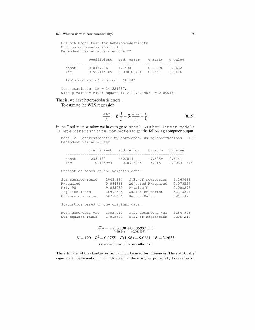
8.3 What to do with heteroscedasticity? 75


coefficient std. error t-ratio p-value--------------------------------------------------------const 0.0457266 1.14381 0.03998 0.9682inc 9.59914e-05 0.000100436 0.9557 0.3416



That is, we have heteroscedastic errors.To estimate the WLS regression

sav

h= β1

1h+β2

inc

h+

uh, (8.19)

in the Gretl main window we have to go to Model→ Other linear models→ Heteroskedasticity corrected to get the following computer output

Model 2: Heteroskedasticity-corrected, using observations 1-100Dependent variable: sav

coefficient std. error t-ratio p-value--------------------------------------------------------const -233.130 460.844 -0.5059 0.6141inc 0.185993 0.0616965 3.015 0.0033 ***

Statistics based on the weighted data:

Sum squared resid 1043.864 S.E. of regression 3.263689R-squared 0.084866 Adjusted R-squared 0.075527F(1, 98) 9.088089 P-value(F) 0.003276Log-likelihood -259.1695 Akaike criterion 522.3391Schwarz criterion 527.5494 Hannan-Quinn 524.4478

Statistics based on the original data:

Mean dependent var 1582.510 S.D. dependent var 3284.902Sum squared resid 1.01e+09 S.E. of regression 3205.216

sav=−233.130(460.84)

+0.185993(0.061697)

inc


The estimates of the standard errors can now be used for inferences. The statisticallysignificant coefficient on inc indicates that the marginal propensity to save out of


your income is 0.18. Of every additional dollar that you make, you will save 18cents.

8.3.4 White’s heteroscedasticity-consistent standard errors

Even under the presence of heteroscedastic errors, at least in large samples a con-sistent estimator of the variances of the coefficients can be obtained via White’sheteroscedasticity-consistent standard errors. This procedure leaves the OLS coef-ficients unaffected. For the estimation of Equation 8.18 you just have to make sureto select the option Robust standard errors in the Gretl “specify model”window when you estimate the model via OLS

Model 3: OLS, using observations 1-100Dependent variable: savHeteroskedasticity-robust standard errors, variant HC1

coefficient std. error t-ratio p-value--------------------------------------------------------const 124.842 528.219 0.2363 0.8137inc 0.146628 0.0613441 2.390 0.0187 **

Mean dependent var 1582.510 S.D. dependent var 3284.902Sum squared resid 1.00e+09 S.E. of regression 3197.415R-squared 0.062127 Adjusted R-squared 0.052557F(1, 98) 5.713342 P-value(F) 0.018748Log-likelihood -947.8935 Akaike criterion 1899.787Schwarz criterion 1904.997 Hannan-Quinn 1901.896

Notice that the constant and slope coefficients are the same as before. However, theestimated standard errors are different.

Chapter 9Binary Choice Models

Some time we are interested in analyzing binary response or qualitative responsevariables that have outcomes Y equal to 1 when the even occurs and equal to 0 whenthe event does not occur. Some example include going to college, getting married,buying a house, or getting a job. All these cases involve a yes/no answer. How is thisyes/no answer affected by other variables? That is the subject matter of this chapter.

9.1 The linear probability model

9.1.1 The model

The simplest binary choice model is the linear probability model, where as its namesuggests, the probability of the event occurring, p, is assumed to be a linear functionof a set of explanatory variable. If we only have one variable the model is

pi = p(Yi = 1) = β1 +β2Xi. (9.1)

The response variable Yi can be written as the summation of its deterministic and itsrandom component,

Yi = E(Yi|Xi)+ui. (9.2)

It is simple to compute E(Yi|Xi), the expected value of Yi given Xi, because Y takesonly two values. It is 1 with probability pi and 0 with probability 1− pi,

E(Yi|Xi) = 1× pi +0× (1− pi) = pi = β1 +β2Xi. (9.3)

This means that we can write the model as

Yi = β1 +β2Xi +ui, (9.4)

77

78 9 Binary Choice Models

that is just the same model we have been estimating in previous chapters. The bigdifference is that Yi takes only the values 0 and 1.

9.1.2 The linear probability model in Gretl

Let’s estimate the following model

inlfi = β1 +β2educi +β3faminci +ui, (9.5)

where inlf is equal to one if individual i is in the labor force, zero otherwise,educ is the number of years of education and faminc is the family income. Theregression command in Gretl is the same as before.

Model 1: OLS, using observations 1-753Dependent variable: inlf

coefficient std. error t-ratio p-value---------------------------------------------------------const 0.0689887 0.0973736 0.7085 0.4789educ 0.0379040 0.00835610 4.536 6.67e-06 ***faminc 1.45940e-06 1.56306e-06 0.9337 0.3508


inlf= 0.0689887(0.097374)

+0.0379040(0.0083561)

educ+1.45940e–006(1.5631e–006)

faminc


For example, the coefficient on educ indicates that every additional years of edu-cation increases the probability of being in the labor force by about 4%. This infor-mation is graphed in Figure 9.1.

There are two main problems with a linear probability model such as the onepresented in Equation 9.4.

1. The model will predict unrealistic probabilities, beyond 1 and below 0 (see Fig-ure 9.1).

2. Because Yi only takes the values of 0 and 1, the error term u will be far fromfollowing a normal distribution.

The solution is to transform the linear probability model. Two common transforma-tions are the logit and the probit.

9.2 Logit analysis 79

Fig. 9.1 inlfi = β1 +β2educi +β3faminci +ui

9.2 Logit analysis

9.2.1 The logit transformation

Let Zi be,Zi = β1 +β2Xi (9.6)

The logit model hypothesizes that the probability of occurrence of the event Y = 1is determined by the function

pi = F(Zi) =1

1+ e−Z (9.7)

where∂ p∂Z

= f (Z) =e−Z

(1+ e−Z)2 (9.8)

and∂ p∂X

=∂ p∂Z

∂Z∂X

= f (Z)β2 (9.9)

This means that the marginal effect of variable X on the probability of Y = 1 isf (Z)β2, where f (Z) needs to be evaluated on some specific value of X , let’s say, themean of X .


9.2.2 Logit regression in Gretl

Fortunately, all these calculations are done automatically by Gretl. If we want toobtain the logit estimates of Equation 9.5 in the main Gretl window we have to goto Model → Nonlinear models → Logit → Binary... and select theoption “Show p-values” to obtain

Convergence achieved after 4 iterations

Model 2: Logit, using observations 1-753Dependent variable: inlf

coefficient std. error z p-value----------------------------------------------------------const -1.85287 0.428444 -4.325 1.53e-05 ***educ 0.161773 0.0367856 4.398 1.09e-05 ***faminc 6.58050e-06 6.83134e-06 0.9633 0.3354

Mean dependent var 0.568393 S.D. dependent var 0.244933McFadden R-squared 0.027185 Adjusted R-squared 0.021359Log-likelihood -500.8762 Akaike criterion 1007.752Schwarz criterion 1021.625 Hannan-Quinn 1013.097

Number of cases ’correctly predicted’ = 449 (59.6%)f(beta’x) at mean of independent vars = 0.245Likelihood ratio test: Chi-square(2) = 27.9939 [0.0000]

Predicted0 1

Actual 0 69 2561 48 380

Gretl actually estimates this model using an estimation technique called MaximumLikelihood Estimation, that is why the computer iterates before giving the esti-mates. The output is very similar as the one obtained in previous chapters. Theeffect of educ on inlf is statistically significant. However, the key difference inthis output is that the coefficients are not interpreted as the marginal effects. Recallthat the marginal effects are calculated using Equation 9.9. To make Gretl obtainthis marginal effects you need to reestimate the model and select the option “Showslopes at mean” to obtain

coefficient std. error z slope-------------------------------------------------------------const -1.85287 0.428444 -4.325educ 0.161773 0.0367856 4.398 0.0396234faminc 6.58050e-06 6.83134e-06 0.9633 1.61178e-06

The marginal effect of educ on inlf is actually 0.0396. An additional year ofeducation will increase the probability that you are in the labor force by about 4%.

9.3 Probit analysis 81

9.3 Probit analysis

9.3.1 The probit transformation

The probit model is similar in spirit as the logit model. Let Zi be,

Zi = β1 +β2Xi (9.10)

The probit model hypothesizes that the probability of occurrence of the event Y = 1is determined by the function

pi = F(Zi) (9.11)

where F(·) is actually the cumulative standardized normal distribution. Then,

∂ p∂Z

= f (Z) =1√2π

e−12 Z2

(9.12)

is just the derivative of F(·). As in the logit case,

∂ p∂X

=∂ p∂Z

∂Z∂X

= f (Z)β2 (9.13)

Again, this means that the marginal effect of variable X on the probability of Y = 1is f (Z)β2, where f (Z) needs to be evaluated on some specific value of X , let’s say,the mean of X .

9.3.2 Probit regression in Gretl

If we want to obtain the probit estimates of Equation 9.5 in the main Gretl windowwe have to go to Model→ Nonlinear models→ Probit→ Binary...and select the option “Show p-values” to obtain

Convergence achieved after 5 iterations

Model 3: Probit, using observations 1-753Dependent variable: inlf

coefficient std. error z p-value----------------------------------------------------------const -1.14768 0.261470 -4.389 1.14e-05 ***educ 0.100666 0.0224296 4.488 7.19e-06 ***faminc 3.84752e-06 4.09647e-06 0.9392 0.3476

Mean dependent var 0.568393 S.D. dependent var 0.392673McFadden R-squared 0.027216 Adjusted R-squared 0.021389Log-likelihood -500.8606 Akaike criterion 1007.721Schwarz criterion 1021.593 Hannan-Quinn 1013.065


Number of cases ’correctly predicted’ = 449 (59.6%)f(beta’x) at mean of independent vars = 0.393Likelihood ratio test: Chi-square(2) = 28.0252 [0.0000]

Predicted0 1

Actual 0 69 2561 48 380

Once again, the effect of educ on inlf is statistically significant. To make Gretlobtain this marginal effects using Equation 9.13 you need to reestimate the modeland select the option “Show slopes at mean” to obtain

coefficient std. error z slope-------------------------------------------------------------const -1.14768 0.261470 -4.389educ 0.100666 0.0224296 4.488 0.0395289faminc 3.84752e-06 4.09647e-06 0.9392 1.51081e-06

The marginal effect of educ on inlf is 0.0395. We obtain almost the same re-sults as before. The probit model predicts that an additional year of education willincrease the probability that you are in the labor force by about 4%.

Chapter 10Time Series

10.1 Time Series Data

The main difference between time series data and cross-sectional data is the tem-poral ordering. To emphasize the proper ordering of the observations, Table 10.1presents a partial listing of the data on U.S. inflation and unemployment rates from1948 through 2003. Unlike cross-sectional data, in time series the temporal order inwhich the observations appear in the data set is very important. In terms of notation,we use the subscript t to denote time and we use it instead of the previous subscripti, i.e., Xt .

Table 10.1 U.S. Inflation and Unemployment Rates, 1965-2011

Year Inflation Unemployment1948 8.1 3.81949 -1.2 5.91950 1.3 5.31951 7.9 3.3

......

...2000 3.4 4.02001 2.8 4.72002 1.6 5.82003 2.3 6.0

A second key difference between time series and cross-sectional data is that in thelatter we assume that the sample was randomly drawn from the population. Whilein time series the variables are also considered random, a variable indexed by timeis called a stochastic process or a time series process. When we collect a time seriesdata set we are one possible outcome or realization of the stochastic process. Wecan only see a single realization because we cannot go back in time and start theprocess again.

83

84 10 Time Series

-2

0

2

4

6

8

10

12

14

1950 1960 1970 1980 1990 2000

Inflation

Fig. 10.1 Inflation, 1948-2003.

Graphing the data is particularly important to visualize the dynamics of the vari-ables. Figure 10.1 presents the time series graph of inflation from 1948 through2003. One can easily identify the periods of high inflation late in the seventies andearly eighties. To obtain this graph in Gretl, go to View→ Graph specifiedvars → Time series plot and then select the variables you want to plotagainst time.

10.2 Time Series Regression Models

10.2.1 Static Models

The simplest static model has the form

Yt = β1 +β2Xt +ut , t = 1,2,3, . . . ,n. (10.1)

10.2 Time Series Regression Models 85

We call this a static model because we are only modeling a contemporaneous rela-tionship between Xt and Yt . That is, when a change in X at time t is believed to havean immediate effect on Y : ∆Yt = β2∆Xt . One example is the static Phillips curvegiven by:

inflationt = β1 +β2unemploymentt +ut . (10.2)

where inflation is the annual inflation rate, and unemployment is the un-employment rate. Estimation in Gretl via OLS is follows the same steps as in theprevious chapters. The output for the estimation of Equation 10.1 is:

Model 1: OLS, using observations 1948-2003 (T = 56)Dependent variable: inflation

coefficient std. error t-ratio p-value----------------------------------------------------------const 1.05357 1.54796 0.6806 0.4990unemployment 0.502378 0.265562 1.892 0.0639 *

Mean dependent var 3.883929 S.D. dependent var 3.040381Sum squared resid 476.8157 S.E. of regression 2.971518R-squared 0.062154 Adjusted R-squared 0.044786F(1, 54) 3.578726 P-value(F) 0.063892Log-likelihood -139.4304 Akaike criterion 282.8607Schwarz criterion 286.9114 Hannan-Quinn 284.4311rho 0.572055 Durbin-Watson 0.801482

inflation= 1.05357(1.5480)

+0.502378(0.26556)

unemployment


The estimation results indicate that a one point increase in the unemployment rateis linked with a 0.5 increase in the inflation rate. Of course more variables can beincluded in the model. Notice that we can use this model to predict inflationgiven that we know the values for unemployment by simply plugging values forunemployment in the estimated equation. If we do this for the actual unemploymentvalues for 1948-2003 period and graph them, we obtain the fitted values graph.Figure 10.2 plots the actual and the fitted values for inflation.

10.2.2 Finite Distributed Lag Models

The simplest dynamic model is the finite distributed lag (FDL) model, where we al-low one or more variables to to affect Yt with a lag. Consider the following example:

Yt = β1 +β2Xt +β3Xt−1 +β4Xt−2 +ut , (10.3)

86 10 Time Series

-2

0

2

4

6

8

10

12

14

1950 1960 1970 1980 1990 2000

Inflation

Year

Actual and fitted inflation

fitted

actual

Fig. 10.2 Inflation, 1948-2003. Actual and fitted based on an static model.

where the FDL is of order two. Let’s say that we are interested in the effect on Yof a permanent increase in X . Before time t, X equals to a constant c. At time t, Xincreases permanently to c+ 1. That is, Xs = c for s < t and Xs = c+ 1 for s ≥ t.Setting the errors to be equal to zero we have:

Yt−1 = β1 +β2c+β3c+β4c (10.4)Yt = β1 +β2(c+1)+β3c+β4c

Yt+1 = β1 +β2(c+1)+β3(c+1)+β4c

Yt+2 = β1 +β2(c+1)+β3(c+1)+β4(c+1)

and so on. The contemporaneous effect of X on Y is called the impact multiplierand in this case this one is given by β2. However, over time the marginal effect of Xon Y is larger. We say that the long-run multiplier is the long-run change Y given apermanent increase in X . This one is given by β2 +β3 +β4.

Consider the following example in Gretl:

inft = β1 +β2unemt +β3unemt−1 +β4unemt−2 +ut , (10.5)


To estimate this model in Gretl we first need to create the lagged values of unem. Todo this we have to go to select unem and then go to Add→ Lags of selectedvariables and select the number of lags. An alternative approach is to just in-clude the lags when estimating the model via OLS. That is, when specifying themodel in Gretl (Model → Ordinary Least Squares) there is an icon thatallows you to select the lags. Just select two lags for unem to obtain:

Model 2: OLS, using observations 1950-2003 (T = 54)Dependent variable: inf

coefficient std. error t-ratio p-value--------------------------------------------------------const -0.124609 1.68922 -0.07377 0.9415unem 0.903211 0.402071 2.246 0.0291 **unem_1 -0.856337 0.525700 -1.629 0.1096unem_2 0.668123 0.386722 1.728 0.0902 *

Mean dependent var 3.900000 S.D. dependent var 2.961323Sum squared resid 395.2340 S.E. of regression 2.811526R-squared 0.149632 Adjusted R-squared 0.098610F(3, 50) 2.932693 P-value(F) 0.042366Log-likelihood -130.3660 Akaike criterion 268.7320Schwarz criterion 276.6880 Hannan-Quinn 271.8003rho 0.661217 Durbin-Watson 0.676987

inf=−0.124609(1.6892)

+0.903211(0.40207)

unem−0.856337(0.52570)

unem 1+0.668123(0.38672)

unem 2


A permanent increase in unemployment leads to a contemporaneous increase ininflation of 0.903 (impact multiplier). However, in the long-run the same increasein unemployment leads to a permanent effect on inflation of 0.903 -0.856 + 0.668 =0.715 (long-run multiplier).

10.2.3 Autoregressive Model

An autoregresive model is a simple model where the current values of a variable arerelated to its past values. The first-order autoregressive model is given by:

Yt = φYt−1 +ut . (10.6)

This one is usually denoted by AR(1). A more general model is the pth autoregres-sive model or AR(p) given by:

Yt = φ1Yt−1 +φ2Yt−2 +φ3Yt−3 + · · ·+φpYt−p +ut (10.7)

88 10 Time Series

where there are p lags of the variable Y explaining its current value. The estimationof an AR(p) model in Gretl is simple; go to Model→ Time series→ ARIMAand then select the dependent variable and the AR order. Make sure that the MAorder is zero. For the example above, consider estimating the following model:

inft = φ1inft−1 +φ2inft−2 +ut (10.8)

The output in Gretl is:

Function evaluations: 17Evaluations of gradient: 8

Model 4: ARMA, using observations 1948-2003 (T = 56)Estimated using Kalman filter (exact ML)Dependent variable: infStandard errors based on Hessian

coefficient std. error z p-value-------------------------------------------------------const 4.02526 0.791433 5.086 3.66e-07 ***phi_1 0.815712 0.148739 5.484 4.15e-08 ***phi_2 -0.175228 0.152459 -1.149 0.2504

Mean dependent var 3.883929 S.D. dependent var 3.040381Mean of innovations -0.054104 S.D. of innovations 2.171763Log-likelihood -123.2506 Akaike criterion 254.5012Schwarz criterion 262.6026 Hannan-Quinn 257.6421

Real Imaginary Modulus Frequency-----------------------------------------------------------AR

Root 1 2.3276 -0.5378 2.3889 -0.0361Root 2 2.3276 0.5378 2.3889 0.0361

-----------------------------------------------------------

That yields the following estimated equation:

inft = 4.025+0.8157inft−1−0.1752inft−2. (10.9)

where we can see that higher inflation last period has a positive effect on inflationthis period. We can use this model to predict the path of inf based on its previousvalues. It Gretl the command to obtain this Graphs→ Fitted, actual plot→ Against time. The resulting graph is shown in Figure 10.3.

10.2.4 Moving-Average Models

The moving-average models express an observed series as a function of the currentand lagged unobserved shocks. The simplest moving-average model is the moving-average of order one, or MA(1):


-2

0

2

4

6

8

10

12

14

1950 1960 1970 1980 1990 2000

inf

Actual and fitted inf

fitted

actual

Fig. 10.3 Inflation, 1948-2003. Actual and fitted based on an AR(2) model.

Yt = θut−1 +ut (10.10)

A more general moving-average of order q is be written as:

Yt = θ1ut−1 +θ2ut−2 +θ3ut−3 + · · ·+θqut−q +ut (10.11)

For the example above:

inft = θ1ut−1 +θ2ut−2 +ut (10.12)

the output in Gretl is:



coefficient std. error z p-value

90 10 Time Series

-4

-2

0

2

4

6

8

10

12

14

1950 1960 1970 1980 1990 2000

inf

Actual and fitted inf

fitted

actual

Fig. 10.4 Inflation, 1948-2003. Actual and fitted based on an MA(2) model.

-------------------------------------------------------const 3.98267 0.615240 6.473 9.58e-011 ***theta_1 1.18549 0.130300 9.098 9.19e-020 ***theta_2 0.267922 0.127516 2.101 0.0356 **


Real Imaginary Modulus Frequency-----------------------------------------------------------MA

Root 1 -1.1343 0.0000 1.1343 0.5000Root 2 -3.2904 0.0000 3.2904 0.5000

-----------------------------------------------------------

and the actual and fitted values are presented in Figure 10.4.


10.2.5 Autoregressive Moving Average Models

One can easily combine an AR(1) model and an MA(1) models to obtain an autore-gressive moving-average model ARMA(1,1):

Yt = φYt−1 +θut−1 +ut (10.13)

or a more general ARMA(p,q) model:

Yt = φ1Yt−1 +φ2Yt−2 + · · ·+φpYt−p +θ1ut−1 +θ2ut−2 + · · ·+θqut−q +ut (10.14)

The output in Gretl for a ARMA(2,2) for inflation is:



coefficient std. error z p-value-------------------------------------------------------const 3.94843 1.05291 3.750 0.0002 ***phi_1 0.828806 0.236639 3.502 0.0005 ***phi_2 0.0226838 0.173277 0.1309 0.8958theta_1 0.274108 0.197397 1.389 0.1650theta_2 -0.587919 0.169467 -3.469 0.0005 ***


Real Imaginary Modulus Frequency-----------------------------------------------------------AR

Root 1 1.1691 0.0000 1.1691 0.0000Root 2 -37.7065 0.0000 37.7065 0.5000

MARoot 1 -1.0917 0.0000 1.0917 0.5000Root 2 1.5580 0.0000 1.5580 0.0000

-----------------------------------------------------------

diego escobari - utrgv

Documents